Tutorial 1. Introduction to Using FLUENT Introduction: This tutorial illustrates the setup and solution of the two-dimensional turbulent fluid flow and heat transfer in a mixing junction. The mixing elbow configuration is encountered in piping systems in power plants and process indus- tries. It is often important to predict the flow field and temperature field in the neighborhood of the mixing region in order to properly design the location of inlet pipes. In this tutorial you will learn how to: • Read an existing grid file into FLUENT • Use mixed units to define the geometry and fluid properties • Set material properties and boundary conditions for a turbulent forced con- vection problem • Initiate the calculation with residual plotting • Calculate a solution using the segregated solver • Examine the flow and temperature fields using graphics • Enable the second-order discretization scheme for improved prediction of tem- perature • Adapt the grid based on the temperature gradient to further improve the prediction of temperature Prerequisites: This tutorial assumes that you have little experience with FLUENT, but that you are generally familiar with the interface. If you are not, please review the sample session in Chapter 1 of the User’s Guide. c Fluent Inc. January 28, 2003 1-1

Welcome message from author
This document is posted to help you gain knowledge. Please leave a comment to let me know what you think about it! Share it to your friends and learn new things together.
Transcript

Tutorial 1. Introduction to Using FLUENT
Introduction: This tutorial illustrates the setup and solution of the two-dimensionalturbulent fluid flow and heat transfer in a mixing junction. The mixing elbowconfiguration is encountered in piping systems in power plants and process indus-tries. It is often important to predict the flow field and temperature field in theneighborhood of the mixing region in order to properly design the location of inletpipes.
In this tutorial you will learn how to:
• Read an existing grid file into FLUENT
• Use mixed units to define the geometry and fluid properties
• Set material properties and boundary conditions for a turbulent forced con-vection problem
• Initiate the calculation with residual plotting
• Calculate a solution using the segregated solver
• Examine the flow and temperature fields using graphics
• Enable the second-order discretization scheme for improved prediction of tem-perature
• Adapt the grid based on the temperature gradient to further improve theprediction of temperature
Prerequisites: This tutorial assumes that you have little experience with FLUENT, butthat you are generally familiar with the interface. If you are not, please review thesample session in Chapter 1 of the User’s Guide.
c© Fluent Inc. January 28, 2003 1-1
Introduction to Using FLUENT
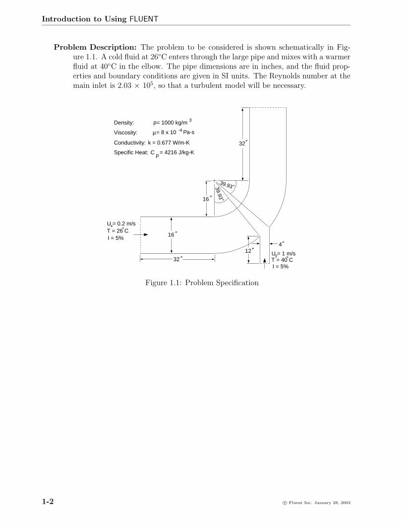
Problem Description: The problem to be considered is shown schematically in Fig-ure 1.1. A cold fluid at 26◦C enters through the large pipe and mixes with a warmerfluid at 40◦C in the elbow. The pipe dimensions are in inches, and the fluid prop-erties and boundary conditions are given in SI units. The Reynolds number at themain inlet is 2.03 × 10⁵, so that a turbulent model will be necessary.
32
12
16
4
″
32 ″
16 ″
″
″″
U = 0.2 m/sT = 26 CI = 5%
U = 1 m/sT = 40 CI = 5%
x
y
°
°
Conductivity: k = 0.677 W/m-K
Density: = 1000 kg/mρ 3
39.93°39.93 °
Viscosity: µ = 8 x 10 -4 Pa-s
pSpecific Heat: C = 4216 J/kg-K
Figure 1.1: Problem Specification
1-2 c© Fluent Inc. January 28, 2003

Introduction to Using FLUENT
Preparation
1. Copy the file elbow/elbow.msh from the FLUENT documentation CD to your work-ing directory.
For UNIX systems, you can find the file by inserting the CD into your CD-ROMdrive and going to the following directory:
/cdrom/fluent6.1/help/tutfiles/
where cdrom must be replaced by the name of your CD-ROM drive.
For Windows systems, you can find the file by inserting the CD into your CD-ROMdrive and going to the following directory:
cdrom:\fluent6.1\help\tutfiles\
where cdrom must be replaced by the name of your CD-ROM drive (e.g., E).
2. Start the 2D version of FLUENT.
c© Fluent Inc. January 28, 2003 1-3

Introduction to Using FLUENT
Step 1: Grid
1. Read the grid file elbow.msh.
File −→ Read −→Case...
(a) Select the file elbow.msh by clicking on it under Files and then clicking on OK.
Note: As this grid is read by FLUENT, messages will appear in the console windowreporting the progress of the conversion. After reading the grid file, FLUENTwill report that 918 triangular fluid cells have been read, along with a numberof boundary faces with different zone identifiers.
2. Check the grid.
Grid −→Check
1-4 c© Fluent Inc. January 28, 2003

Introduction to Using FLUENT
Grid Check
Domain Extents:x-coordinate: min (m) = 0.000000e+00, max (m) = 6.400001e+01y-coordinate: min (m) = -4.538534e+00, max (m) = 6.400000e+01
Volume statistics:minimum volume (m3): 2.782193e-01maximum volume (m3): 3.926232e+00
total volume (m3): 1.682930e+03Face area statistics:minimum face area (m2): 8.015718e-01maximum face area (m2): 4.118252e+00
Checking number of nodes per cell.Checking number of faces per cell.Checking thread pointers.Checking number of cells per face.Checking face cells.Checking bridge faces.Checking right-handed cells.Checking face handedness.Checking element type consistency.Checking boundary types:Checking face pairs.Checking periodic boundaries.Checking node count.Checking nosolve cell count.Checking nosolve face count.Checking face children.Checking cell children.Checking storage.Done.
Note: The grid check lists the minimum and maximum x and y values from thegrid, in the default SI units of meters, and reports on a number of other gridfeatures that are checked. Any errors in the grid would be reported at this time.In particular, you should always make sure that the minimum volume is notnegative, since FLUENT cannot begin a calculation if this is the case. To scalethe grid to the correct units of inches, the Scale Grid panel will be used.
c© Fluent Inc. January 28, 2003 1-5

Introduction to Using FLUENT
3. Smooth (and swap) the grid.
Grid −→ Smooth/Swap...
To ensure the best possible grid quality for the calculation, it is good practice tosmooth a triangular or tetrahedral grid after you read it into FLUENT.
(a) Click the Smooth button and then click Swap repeatedly until FLUENT reportsthat zero faces were swapped.
If FLUENT cannot improve the grid by swapping, no faces will be swapped.
(b) Close the panel.
4. Scale the grid.
Grid −→Scale...
(a) Under Units Conversion, select in from the drop-down list to complete thephrase Grid Was Created In in (inches).
(b) Click Scale to scale the grid.
The reported values of the Domain Extents will be reported in the default SIunits of meters.
(c) Click Change Length Units to set inches as the working units for length.
Confirm that the maximum x and y values are 64 inches (see Figure 1.1).
1-6 c© Fluent Inc. January 28, 2003

Introduction to Using FLUENT
(d) The grid is now sized correctly, and the working units for length have beenset to inches. Close the panel.
Note: Because the default SI units will be used for everything but the length, therewill be no need to change any other units in this problem. The choice of inchesfor the unit of length has been made by the actions you have just taken. If youwant to change the working units for length to something other than inches,say, mm, you would have to visit the Set Units panel in the Define pull-downmenu.
5. Display the grid (Figure 1.2).
Display −→Grid...
(a) Make sure that all of the surfaces are selected and click Display.
c© Fluent Inc. January 28, 2003 1-7

Introduction to Using FLUENT
GridFLUENT 6.1 (2d, segregated, lam)
Nov 13, 2002
Figure 1.2: The Triangular Grid for the Mixing Elbow
Extra: You can use the right mouse button to check which zone number corresponds toeach boundary. If you click the right mouse button on one of the boundaries in thegraphics window, its zone number, name, and type will be printed in the FLUENTconsole window. This feature is especially useful when you have several zones ofthe same type and you want to distinguish between them quickly.
1-8 c© Fluent Inc. January 28, 2003

Introduction to Using FLUENT
Step 2: Models
1. Keep the default solver settings.
Define −→ Models −→Solver...
2. Turn on the standard k-ε turbulence model.
Define −→ Models −→Viscous...
(a) Select k-epsilon in the Model list.
The original Viscous Model panel will expand when you do so.
(b) Accept the default Standard model by clicking OK.
c© Fluent Inc. January 28, 2003 1-9

Introduction to Using FLUENT
3. Enable heat transfer by activating the energy equation.
Define −→ Models −→Energy...
1-10 c© Fluent Inc. January 28, 2003

Introduction to Using FLUENT
Step 3: Materials
1. Create a new material called water.
Define −→Materials...
(a) Type the name water in the Name text-entry box.
(b) Enter the values shown in the table below under Properties:
Property Valuedensity 1000 kg/m3
cp 4216 J/kg-Kthermal conductivity 0.677 W/m-Kviscosity 8 ×10⁻⁴ kg/m-s
(c) Click Change/Create.
(d) Click No when FLUENT asks if you want to overwrite air.
The material water will be added to the list of materials which originally con-tained only air. You can confirm that there are now two materials defined byexamining the drop-down list under Fluid Materials.
c© Fluent Inc. January 28, 2003 1-11

Introduction to Using FLUENT
Extra: You could have copied the material water from the materials database(accessed by clicking on the Database... button). If the properties in thedatabase are different from those you wish to use, you can still edit thevalues under Properties and click the Change/Create button to update yourlocal copy. (The database will not be affected.)
(e) Close the Materials panel.
1-12 c© Fluent Inc. January 28, 2003
Introduction to Using FLUENT
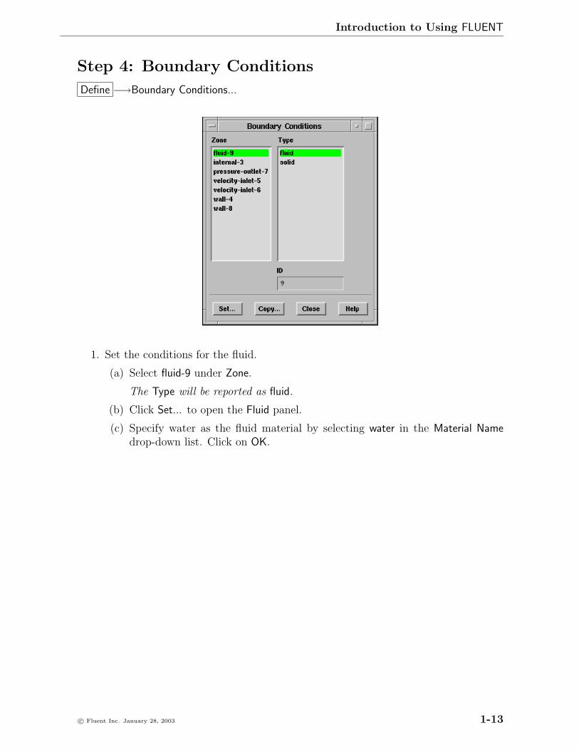
Step 4: Boundary Conditions
Define −→Boundary Conditions...
1. Set the conditions for the fluid.
(a) Select fluid-9 under Zone.
The Type will be reported as fluid.
(b) Click Set... to open the Fluid panel.
(c) Specify water as the fluid material by selecting water in the Material Namedrop-down list. Click on OK.
c© Fluent Inc. January 28, 2003 1-13

Introduction to Using FLUENT
2. Set the boundary conditions at the main inlet.
(a) Select velocity-inlet-5 under Zone and click Set....
Hint: If you are unsure of which inlet zone corresponds to the main inlet,you can probe the grid display with the right mouse button and the zoneID will be displayed in the FLUENT console window. In the BoundaryConditions panel, the zone that you probed will automatically be selectedin the Zone list. In 2D simulations, it may be helpful to return to the GridDisplay panel and deselect the display of the fluid and interior zones (inthis case, fluid-9 and internal-3) before probing with the mouse button forzone names.
1-14 c© Fluent Inc. January 28, 2003

Introduction to Using FLUENT
(b) Choose Components as the Velocity Specification Method.
(c) Set an X-Velocity of 0.2 m/s.
(d) Set a Temperature of 293 K.
(e) Select Intensity and Hydraulic Diameter as the Turbulence Specification Method.
(f) Enter a Turbulence Intensity of 5%, and a Hydraulic Diameter of 32 in.
3. Repeat this operation for velocity-inlet-6, using the values in the following table:
velocity specification method componentsy velocity 1.0 m/stemperature 313 Kturbulence specification method intensity & hydraulic diameterturbulence intensity 5%hydraulic diameter 8 in
c© Fluent Inc. January 28, 2003 1-15

Introduction to Using FLUENT
4. Set the boundary conditions for pressure-outlet-7, as shown in the panel below.
These values will be used in the event that flow enters the domain through thisboundary.
5. For wall-4, keep the default settings for a Heat Flux of 0.
1-16 c© Fluent Inc. January 28, 2003

Introduction to Using FLUENT
6. For wall-8, you will also keep the default settings.
Note: If you probe your display of the grid (without the interior cells) you will seethat wall-8 is the wall on the outside of the bend just after the junction. Thisseparate wall zone has been created for the purpose of doing certain postpro-cessing tasks, to be discussed later in this tutorial.
c© Fluent Inc. January 28, 2003 1-17

Introduction to Using FLUENT
Step 5: Solution
1. Initialize the flow field using the boundary conditions set at velocity-inlet-5.
Solve −→ Initialize −→Initialize...
(a) Choose velocity-inlet-5 from the Compute From list.
(b) Add a Y Velocity value of 0.2 m/sec throughout the domain.
Note: While an initial X Velocity is an appropriate guess for the horizontalsection, the addition of a Y Velocity will give rise to a better initial guessthroughout the entire elbow.
(c) Click Init and Close the panel.
1-18 c© Fluent Inc. January 28, 2003

Introduction to Using FLUENT
2. Enable the plotting of residuals during the calculation.
Solve −→ Monitors −→Residual...
(a) Select Plot under Options, and click OK.
Note: By default, all variables will be monitored and checked for determining theconvergence of the solution.
c© Fluent Inc. January 28, 2003 1-19

Introduction to Using FLUENT
3. Save the case file (elbow1.cas).
File −→ Write −→Case...
Keep the Write Binary Files (default) option on so that a binary file will be written.
4. Start the calculation by requesting 100 iterations.
Solve −→Iterate...
(a) Input 100 for the Number of Iterations and click Iterate.
The solution reaches convergence after approximately 60 iterations. The resid-ual plot is shown in Figure 1.3. Note that since the residual values are differentfor different computers, the plot that appears on your screen may not be exactlythe same as the one shown here.
1-20 c© Fluent Inc. January 28, 2003

Introduction to Using FLUENT
Scaled ResidualsFLUENT 6.1 (2d, segregated, ske)
Nov 12, 2002
Iterations
6050403020100
1e+03
1e+02
1e+01
1e+00
1e-01
1e-02
1e-03
1e-04
1e-05
1e-06
1e-07
epsilonkenergyy-velocityx-velocitycontinuityResiduals
Figure 1.3: Residuals for the First 60 Iterations
5. Check for convergence.
There are no universal metrics for judging convergence. Residual definitions thatare useful for one class of problem are sometimes misleading for other classes ofproblems. Therefore it is a good idea to judge convergence not only by examiningresidual levels, but also by monitoring relevant integrated quantities and checkingfor mass and energy balances.
The three methods to check for convergence are:
• Monitoring the residuals.
Convergence will occur when the Convergence Criterion for each variable hasbeen reached. The default criterion is that each residual will be reduced toa value of less than 10−3, except the energy residual, for which the defaultcriterion is 10−6.
• Solution no longer changes with more iterations.
Sometimes the residuals may not fall below the convergence criterion set inthe case setup. However, monitoring the representative flow variables throughiterations may show that the residuals have stagnated and do not change withfurther iterations. This could also be considered as convergence.
c© Fluent Inc. January 28, 2003 1-21

Introduction to Using FLUENT
• Overall mass, momentum, energy and scalar balances are obtained.
Check the overall mass, momentum, energy and scalar balances in the FluxReports panel. The net imbalance should be less than 0.1% of the net fluxthrough the domain.
Report −→Fluxes
6. Save the data file (elbow1.dat).
Use the same prefix (elbow1) that you used when you saved the case file earlier.Note that additional case and data files will be written later in this session.
File −→ Write −→Data...
1-22 c© Fluent Inc. January 28, 2003
Introduction to Using FLUENT
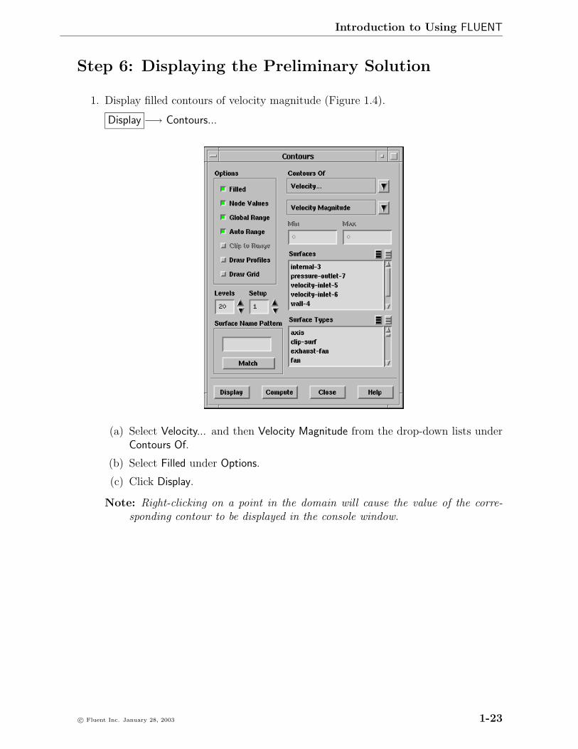
Step 6: Displaying the Preliminary Solution
1. Display filled contours of velocity magnitude (Figure 1.4).
Display −→ Contours...
(a) Select Velocity... and then Velocity Magnitude from the drop-down lists underContours Of.
(b) Select Filled under Options.
(c) Click Display.
Note: Right-clicking on a point in the domain will cause the value of the corre-sponding contour to be displayed in the console window.
c© Fluent Inc. January 28, 2003 1-23

Introduction to Using FLUENT
Contours of Velocity Magnitude (m/s)FLUENT 6.1 (2d, segregated, ske)
Nov 12, 2002
1.24e+001.18e+001.12e+001.05e+009.93e-019.31e-018.69e-018.07e-017.45e-016.82e-016.20e-015.58e-014.96e-014.34e-013.72e-013.10e-012.48e-011.86e-011.24e-016.20e-020.00e+00
Figure 1.4: Predicted Velocity Distribution After the Initial Calculation
1-24 c© Fluent Inc. January 28, 2003

Introduction to Using FLUENT
2. Display filled contours of temperature (Figure 1.5).
(a) Select Temperature... and Static Temperature in the drop-down lists underContours Of.
(b) Click Display.
c© Fluent Inc. January 28, 2003 1-25

Introduction to Using FLUENT
Contours of Static Temperature (k)FLUENT 6.1 (2d, segregated, ske)
Nov 12, 2002
3.13e+023.12e+023.11e+023.10e+023.09e+023.08e+023.07e+023.06e+023.05e+023.04e+023.03e+023.02e+023.01e+023.00e+022.99e+022.98e+022.97e+022.96e+022.95e+022.94e+022.93e+02
Figure 1.5: Predicted Temperature Distribution After the Initial Calculation
1-26 c© Fluent Inc. January 28, 2003

Introduction to Using FLUENT
3. Display velocity vectors (Figure 1.6).
Display −→ Vectors...
(a) Click Display to plot the velocity vectors.
Note: The Auto Scale button is on by default under Options. This scalingsometimes creates vectors that are too small or too large in the majorityof the domain.
(b) Resize the vectors by increasing the Scale factor to 3.
(c) Display the vectors once again.
(d) Use the middle mouse button to zoom the view. To do this, hold down thebutton and drag your mouse to the right and either up or down to constructa rectangle on the screen. The rectangle should be a frame around the regionthat you wish to enlarge. Let go of the mouse button and the image will beredisplayed (Figure 1.7).
(e) Un-zoom the view by holding down the middle mouse button and dragging itto the left to create a rectangle. When you let go, the image will be redrawn.If the resulting image is not centered, you can use the left mouse button totranslate it on your screen.
c© Fluent Inc. January 28, 2003 1-27

Introduction to Using FLUENT
Velocity Vectors Colored By Velocity Magnitude (m/s)FLUENT 6.1 (2d, segregated, ske)
Nov 12, 2002
1.40e+001.33e+001.27e+001.20e+001.13e+001.06e+009.96e-019.28e-018.61e-017.93e-017.26e-016.59e-015.91e-015.24e-014.56e-013.89e-013.21e-012.54e-011.86e-011.19e-015.16e-02
Figure 1.6: Resized Velocity Vectors
Velocity Vectors Colored By Velocity Magnitude (m/s)FLUENT 6.1 (2d, segregated, ske)
Nov 13, 2002
1.40e+001.33e+001.27e+001.20e+001.13e+001.06e+009.96e-019.28e-018.61e-017.93e-017.26e-016.59e-015.91e-015.24e-014.56e-013.89e-013.21e-012.54e-011.86e-011.19e-015.16e-02
Figure 1.7: Magnified View of Velocity Vectors
1-28 c© Fluent Inc. January 28, 2003

Introduction to Using FLUENT
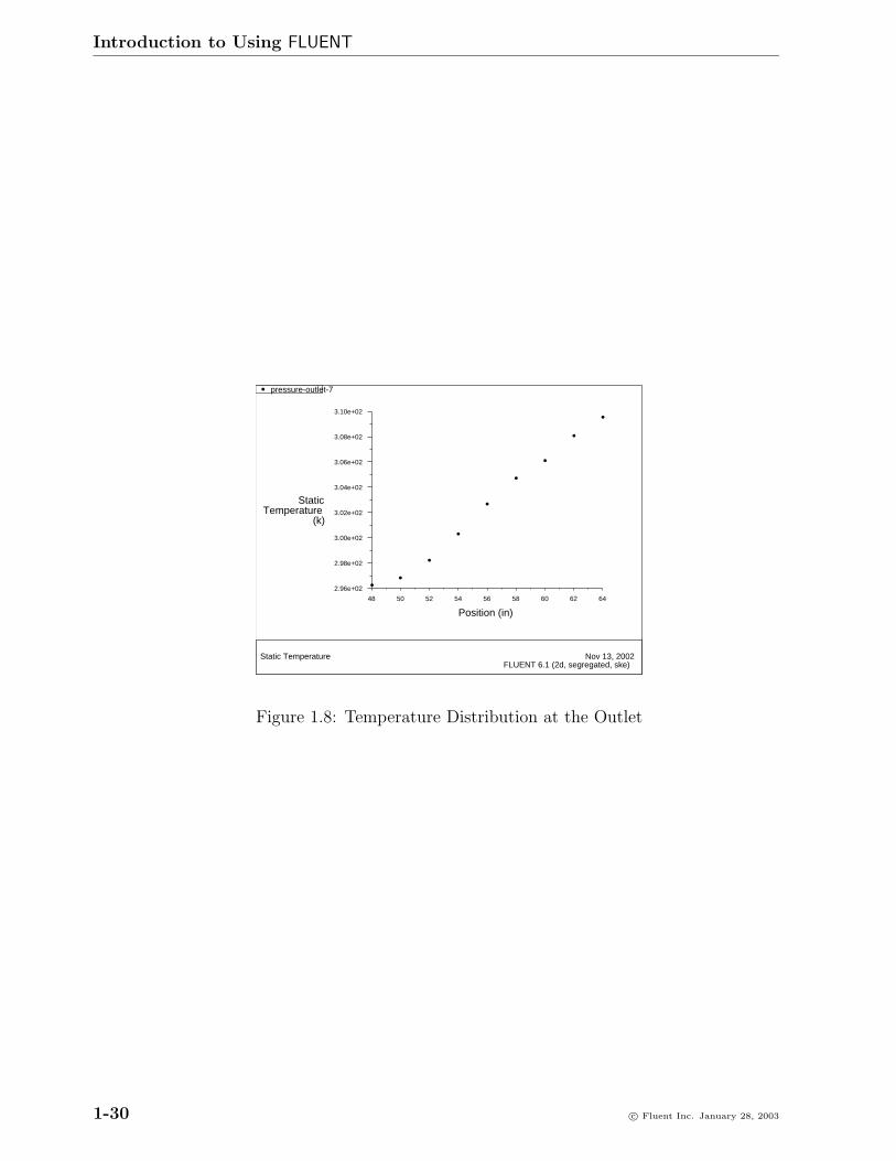
4. Create an XY plot of temperature across the exit (Figure 1.8).
Plot −→ XY Plot...
(a) Select Temperature... and Static Temperature in the drop-down lists under theY Axis Function.
(b) Select pressure-outlet-7 from the Surfaces list.
(c) Click Plot.
c© Fluent Inc. January 28, 2003 1-29
Introduction to Using FLUENT
Static TemperatureFLUENT 6.1 (2d, segregated, ske)
Nov 13, 2002
Position (in)
(k)Temperature
Static
646260585654525048
3.10e+02
3.08e+02
3.06e+02
3.04e+02
3.02e+02
3.00e+02
2.98e+02
2.96e+02
pressure-outlet-7
Figure 1.8: Temperature Distribution at the Outlet
1-30 c© Fluent Inc. January 28, 2003

Introduction to Using FLUENT
5. Make an XY plot of the static pressure on the outer wall of the large pipe, wall-8(Figure 1.9).
(a) Choose Pressure... and Static Pressure from the Y Axis Function drop-downlists.
(b) Deselect pressure-outlet-7 and select wall-8 from the Surfaces list.
(c) Change the Plot Direction for X to 0, and the Plot Direction for Y to 1.
With a Plot Direction vector of (0,1), FLUENT will plot static pressure at thecells of wall-8 as a function of y.
(d) Click Plot.
c© Fluent Inc. January 28, 2003 1-31

Introduction to Using FLUENT
Static PressureFLUENT 6.1 (2d, segregated, ske)
Nov 13, 2002
Position (in)
(pascal)Pressure
Static
70605040302010
1.00e+02
0.00e+00
-1.00e+02
-2.00e+02
-3.00e+02
-4.00e+02
-5.00e+02
-6.00e+02
wall-8
Figure 1.9: Pressure Distribution along the Outside Wall of the Bend
1-32 c© Fluent Inc. January 28, 2003

Introduction to Using FLUENT
6. Define a custom field function for the dynamic head formula (ρ|V |2/2).
Define −→ Custom Field Functions...
(a) In the Field Functions drop-down list, select Density and click the Select button.
(b) Click the multiplication button, X.
(c) In the Field Functions drop-down list, select Velocity and Velocity Magnitudeand click Select.
(d) Click y^x to raise the last entry to a power, and click 2 for the power.
(e) Click the divide button, /, and then click 2.
(f) Enter the name dynam-head in the New Function Name text entry box.
(g) Click Define, and then Close the panel.
c© Fluent Inc. January 28, 2003 1-33

Introduction to Using FLUENT
7. Display filled contours of the custom field function (Figure 1.10).
Display −→ Contours...
(a) Select Custom Field Functions... in the drop-down list under Contours Of.
The function you created, dynam-head, will be shown in the lower drop-downlist.
(b) Click Display, and then Close the panel.
Note: You may need to un-zoom your view after the last vector display, if you havenot already done so.
1-34 c© Fluent Inc. January 28, 2003

Introduction to Using FLUENT
Contours of dynam-headFLUENT 6.1 (2d, segregated, ske)
Nov 13, 2002
7.69e+027.30e+026.92e+026.53e+026.15e+025.76e+025.38e+025.00e+024.61e+024.23e+023.84e+023.46e+023.07e+022.69e+022.31e+021.92e+021.54e+021.15e+027.69e+013.84e+010.00e+00
Figure 1.10: Contours of the Custom Field Function, Dynamic Head
c© Fluent Inc. January 28, 2003 1-35
Introduction to Using FLUENT
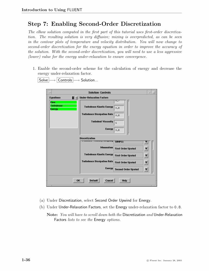
Step 7: Enabling Second-Order Discretization
The elbow solution computed in the first part of this tutorial uses first-order discretiza-tion. The resulting solution is very diffusive; mixing is overpredicted, as can be seenin the contour plots of temperature and velocity distribution. You will now change tosecond-order discretization for the energy equation in order to improve the accuracy ofthe solution. With the second-order discretization, you will need to use a less aggressive(lower) value for the energy under-relaxation to ensure convergence.
1. Enable the second-order scheme for the calculation of energy and decrease theenergy under-relaxation factor.
Solve −→ Controls −→ Solution...
(a) Under Discretization, select Second Order Upwind for Energy.
(b) Under Under-Relaxation Factors, set the Energy under-relaxation factor to 0.8.
Note: You will have to scroll down both the Discretization and Under-RelaxationFactors lists to see the Energy options.
1-36 c© Fluent Inc. January 28, 2003

Introduction to Using FLUENT
2. Continue the calculation by requesting 100 more iterations.
Solve −→ Iterate...
The solution converges in approximately 35 additional iterations.
Scaled ResidualsFLUENT 6.1 (2d, segregated, ske)
Nov 12, 2002
Iterations
9080706050403020100
1e+03
1e+02
1e+01
1e+00
1e-01
1e-02
1e-03
1e-04
1e-05
1e-06
1e-07
epsilonkenergyy-velocityx-velocitycontinuityResiduals
Figure 1.11: Residuals for the Second-Order Energy Calculation
Note: Whenever you change the solution control parameters, it is natural to seethe residuals jump.
c© Fluent Inc. January 28, 2003 1-37

Introduction to Using FLUENT
3. Write the case and data files for the second-order solution (elbow2.cas and elbow2.dat).
File −→ Write −→ Case & Data...
(a) Enter the name elbow2 in the Case/Data File box.
(b) Click OK.
The files elbow2.cas and elbow2.dat will be created in your directory.
4. Examine the revised temperature distribution (Figure 1.12).
Display −→ Contours...
The thermal spreading after the elbow has been reduced from the earlier prediction(Figure 1.5).
1-38 c© Fluent Inc. January 28, 2003

Introduction to Using FLUENT
Contours of Static Temperature (k)FLUENT 6.1 (2d, segregated, ske)
Nov 12, 2002
3.13e+023.12e+023.11e+023.10e+023.09e+023.08e+023.07e+023.06e+023.04e+023.03e+023.02e+023.01e+023.00e+022.99e+022.98e+022.97e+022.96e+022.95e+022.94e+022.93e+022.92e+02
Figure 1.12: Temperature Contours for the Second-Order Solution
c© Fluent Inc. January 28, 2003 1-39

Introduction to Using FLUENT
Step 8: Adapting the Grid
The elbow solution can be improved further by refining the grid to better resolve the flowdetails. In this step, you will adapt the grid based on the temperature gradients in thecurrent solution. Before adapting the grid, you will first determine an acceptable rangeof temperature gradients over which to adapt. Once the grid has been refined, you willcontinue the calculation.
1. Plot filled contours of temperature on a cell-by-cell basis (Figure 1.13).
Display −→ Contours...
(a) Select Temperature... and Static Temperature in the Contours Of drop-downlists.
(b) Deselect Node Values under Options and click Display.
Note: When the contours are displayed you will see the cell values of temper-ature instead of the smooth-looking node values. Node values are obtainedby averaging the values at all of the cells that share the node. Cell val-ues are the values that are stored at each cell center and are displayedthroughout the cell. Examining the cell-by-cell values is helpful when youare preparing to do an adaption of the grid because it indicates the re-gion(s) where the adaption will take place.
1-40 c© Fluent Inc. January 28, 2003

Introduction to Using FLUENT
2. Plot the temperature gradients that will be used for adaption (Figure 1.14).
(a) Select Adaption... and Adaption Function in the Contours Of drop-down lists.
(b) Click Display to see the gradients of temperature, displayed on a cell-by-cellbasis.
Contours of Static Temperature (k)FLUENT 6.1 (2d, segregated, ske)
Nov 12, 2002
3.13e+023.12e+023.11e+023.10e+023.08e+023.07e+023.06e+023.05e+023.04e+023.03e+023.02e+023.01e+022.99e+022.98e+022.97e+022.96e+022.95e+022.94e+022.93e+022.91e+022.90e+02
Figure 1.13: Temperature Contours for the Second-Order Solution: Cell Values
c© Fluent Inc. January 28, 2003 1-41

Introduction to Using FLUENT
Contours of Adaption FunctionFLUENT 6.1 (2d, segregated, ske)
Nov 12, 2002
1.30e-011.23e-011.17e-011.10e-011.04e-019.74e-029.09e-028.44e-027.79e-027.14e-026.49e-025.84e-025.20e-024.55e-023.90e-023.25e-022.60e-021.95e-021.30e-026.49e-031.42e-14
Figure 1.14: Contours of Adaption Function: Temperature Gradient
Note: The quantity Adaption Function defaults to the gradient of the variablewhose Max and Min were most recently computed in the Contours panel.In this example, the static temperature is the most recent variable to haveits Max and Min computed, since this occurs when the Display button ispushed. Note that for other applications, gradients of another variablemight be more appropriate for performing the adaption.
3. Plot temperature gradients over a limited range in order to mark cells for adaption(Figure 1.15).
(a) Under Options, deselect Auto Range so that you can change the minimumtemperature gradient value to be plotted.
The Min temperature gradient is 0 K/m, as shown in the Contours panel.
(b) Enter a new Min value of 0.02.
(c) Click Display.
The colored cells in the figure are in the “high gradient” range, so they will bethe ones targeted for adaption.
4. Adapt the grid in the regions of high temperature gradient.
Adapt −→ Gradient...
(a) Select Temperature... and Static Temperature in the Gradients Of drop-downlists.
(b) Deselect Coarsen under Options, so that only a refinement of the grid will beperformed.
1-42 c© Fluent Inc. January 28, 2003

Introduction to Using FLUENT
Contours of Adaption FunctionFLUENT 6.1 (2d, segregated, ske)
Nov 12, 2002
1.30e-011.24e-011.19e-011.13e-011.08e-011.02e-019.69e-029.14e-028.59e-028.04e-027.49e-026.94e-026.40e-025.85e-025.30e-024.75e-024.20e-023.65e-023.10e-022.55e-022.00e-02
Figure 1.15: Contours of Temperature Gradient Over a Limited Range
(c) Click Compute.
FLUENT will update the Min and Max values.
(d) Enter the value of 0.02 for the Refine Threshold.
c© Fluent Inc. January 28, 2003 1-43
Introduction to Using FLUENT
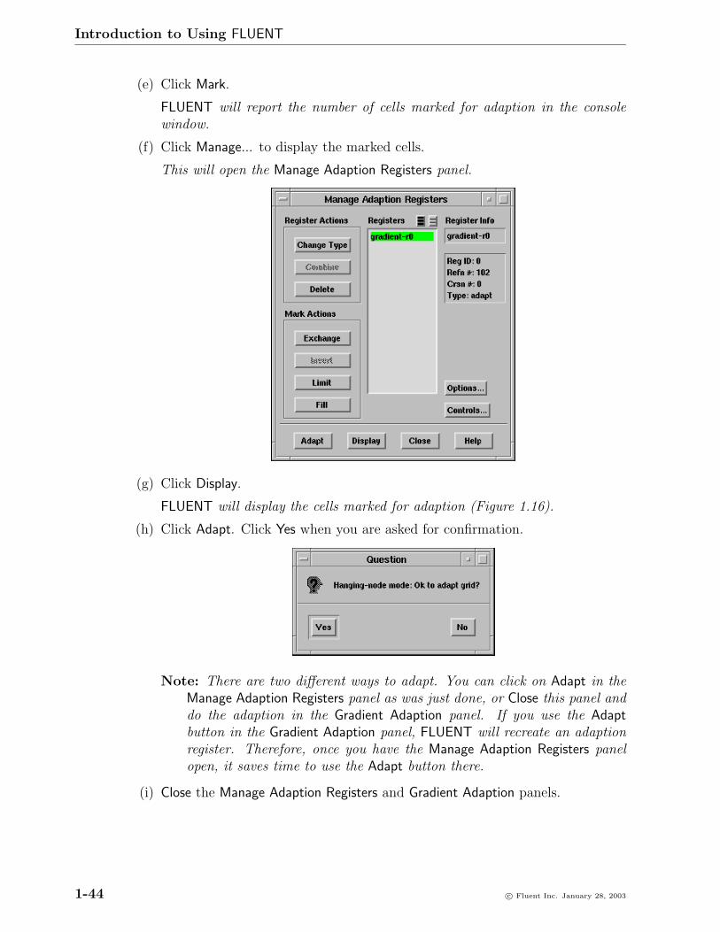
(e) Click Mark.
FLUENT will report the number of cells marked for adaption in the consolewindow.
(f) Click Manage... to display the marked cells.
This will open the Manage Adaption Registers panel.
(g) Click Display.
FLUENT will display the cells marked for adaption (Figure 1.16).
(h) Click Adapt. Click Yes when you are asked for confirmation.
Note: There are two different ways to adapt. You can click on Adapt in theManage Adaption Registers panel as was just done, or Close this panel anddo the adaption in the Gradient Adaption panel. If you use the Adaptbutton in the Gradient Adaption panel, FLUENT will recreate an adaptionregister. Therefore, once you have the Manage Adaption Registers panelopen, it saves time to use the Adapt button there.
(i) Close the Manage Adaption Registers and Gradient Adaption panels.
1-44 c© Fluent Inc. January 28, 2003

Introduction to Using FLUENT
Adaption Markings (gradient-r0)FLUENT 6.1 (2d, segregated, ske)
Nov 12, 2002
Figure 1.16: Cells Marked for Adaption
c© Fluent Inc. January 28, 2003 1-45

Introduction to Using FLUENT
5. Display the adapted grid (Figure 1.17).
Display −→ Grid...
GridFLUENT 6.1 (2d, segregated, ske)
Nov 12, 2002
Figure 1.17: The Adapted Grid
6. Request an additional 100 iterations.
Solve −→ Iterate...
The solution converges after approximately 40 additional iterations.
7. Write the final case and data files (elbow3.cas and elbow3.dat) using the prefixelbow3.
File −→ Write −→ Case & Data...
1-46 c© Fluent Inc. January 28, 2003

Introduction to Using FLUENT
Scaled ResidualsFLUENT 6.1 (2d, segregated, ske)
Nov 12, 2002
Iterations
140120100806040200
1e+03
1e+02
1e+01
1e+00
1e-01
1e-02
1e-03
1e-04
1e-05
1e-06
1e-07
epsilonkenergyy-velocityx-velocitycontinuityResiduals
Figure 1.18: The Complete Residual History
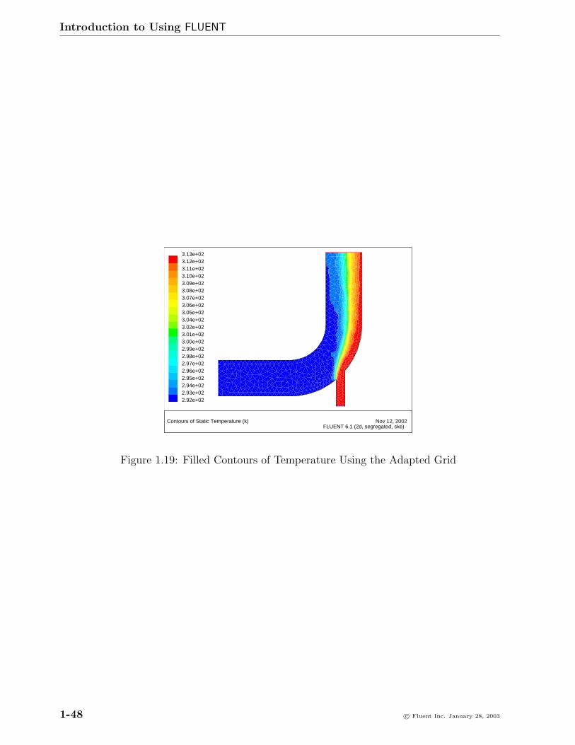
8. Examine the filled temperature distribution (using node values) on the revised grid(Figure 1.19).
Display −→ Contours...
Summary: Comparison of the filled temperature contours for the first solution (us-ing the original grid and first-order discretization) and the last solution (using anadapted grid and second-order discretization) clearly indicate that the latter is muchless diffusive. While first-order discretization is the default scheme in FLUENT, itis good practice to use your first-order solution as a starting guess for a calculationthat uses a higher-order discretization scheme and, optionally, an adapted grid.
Note that in this problem, the flow field is decoupled from temperature since allproperties are constant. For such cases, it is more efficient to compute the flow-fieldsolution first (i.e., without solving the energy equation) and then solve for energy(i.e., without solving the flow equations). You will use the Solution Controls panelto turn solution of the equations on and off during this procedure.
c© Fluent Inc. January 28, 2003 1-47
Introduction to Using FLUENT
Contours of Static Temperature (k)FLUENT 6.1 (2d, segregated, ske)
Nov 12, 2002
3.13e+023.12e+023.11e+023.10e+023.09e+023.08e+023.07e+023.06e+023.05e+023.04e+023.02e+023.01e+023.00e+022.99e+022.98e+022.97e+022.96e+022.95e+022.94e+022.93e+022.92e+02
Figure 1.19: Filled Contours of Temperature Using the Adapted Grid
1-48 c© Fluent Inc. January 28, 2003
Related Documents