Turbulent properties in a homogeneous tidal bottom boundary layer

JOURNAL OF GEOPHYSICAL RESEARCH, VOL. 104, NO. C1, PAGES 1245-1257, JANUARY 15, 1999

Turbulent properties in a homogeneous tidal bottom boundary layer

Thomas B. Sanford and Ren-Chieh Lien

Applied Physics Laboratory and School of Oceanography, College of Ocean and Fishery Sciences University of Washington, Seattle

Abstract. Profiles of mean and turbulent velocity and vorticity in a tidal bottom boundary layer are reported. Friction velocities estimated (1) by the profile method using the time mean streamwise velocity, (2) by the eddy-correlation method using the turbulent Reynolds stress, and (3) by the dissipation method using the turbulent kinetic energy dissipation rate e are in good agreement. The mean streamwise velocity component exhibits two distinct log layers. In both layers, e is inversely proportional to the distance from the bottom Z. The lower log layer occupies the bottom 3 m. In this layer, the turbulent Reynolds stress is nearly constant. The dynamics in the lower log layer are directly related to the stress induced by the seabed. The upper log layer spans 5 to 12 m above the bottom. In this layer, the turbulent Reynolds stress decreases toward the surface. The friction velocity estimated by the profile method in the upper log layer is about 1.8 times of that estimated in the lower log layer. Form drag might be important in the upper log layer. A detailed study of upstream topography is required for the bed stress estimate. The mean profile of vertical flux of spanwise vorticity is nearly uniform with Z and is at least a factor of 5 larger than the vertical divergence of turbulent Reynolds stress to which it may be compared. A new method of estimating the friction velocity is proposed that uses the vertical flux of turbulent spanwise vorticity. This is supported by the fact that the vertical eddy diffusivity for the turbulent vorticity is about equal in magnitude and vertical structure to the eddy viscosity for the turbulent momentum. The friction velocity calculated from the vorticity flux is equal to that estimated by the other three methods. Turbulent enstrophy, corrected for the sensor response function, is proportional to Z -1 for the entire water column. The relation between e and enstrophy for high-Reynolds-number flows is confirmed by our observations.

1. Introduction

Studies of estuarine and coastal oceans require es- timates of stress induced by the seabed to quantify the transport of bottom sediment and provide bottom boundary conditions for numerical models. It is rel- atively di•cult to determine the bed stress directly in the field because it requires measurements very near the bottom. In practice, seabed stress is often inferred from measurements of the mean flow or turbulent properties well above the seabed, based on the characteristics of the turbulent boundary layer. Previous studies have found discrepancies in the seabed stress estimated by different methods [Chriss and Caldwell, 1982; Dewey and Crawford, 1988; Johnson et al., 1994]. Possible explanations for these discrepancies include invalid as- sumptions about the turbulent kinetic energy budget in

Copyright 1999 by the American Geophysical Union.

Paper number 1998JC900068. 0148-0227/99/1998 JC900068 $09.00

the turbulent boundary layer, measurement errors, and the extra stress due to form drag produced by bottom topography. Sediment suspension and deposition may change bottom topography. A better understanding of the turbulent boundary layer is needed to resolve the observed contradictions and obtain a'reliable estimate of seabed stress.

In the turbulent boundary layer, vorticity plays an important role in dynamics. Vorticity is fundamen- tally connected with the turbulent kinetic energy dis- sipation rate s, momentum flux, and seabed processes. In high-Reynolds-number flows, the variance of vor- ticity (enstrophy), /• •- •), is proportional to s, i.e., • = F(•-(j•), where angle brackets denote the ensem- ble average and F is the kinematic molecular viscosity [Saffman, 1980]. Laboratory experiments and numeri- cal simulations have found coherent vortical motions in

turbulent boundary layers [Robinson, 1991]. Vorticity dynamics are related to momentum flux in the turbu- lent boundary layer via sweeping and ejection events [Kim et al., 1971; Willmarth and Lu, 1972; Blackwelder

1245

1246 SANFORD AND LIEN ß TURBULENCE IN A TIDAL BOUNDARY LAYER

and Eckelmann, 1979]. The sweeping process is associ- ated with the creation of new vortices [Bernard et al., 1993]. Tilted vortex cores accelerate fluid particles trav- eling toward the wall region and decelerate fluid parti- cles leaving the wall region, thereby providing a mecha- nism for production of Reynolds stress. The divergence of the turbulent momentum flux can be expressed by the associated vorticity fluxes via a kinematic relation. In a laboratory experiment, Klewicki et al. [1994] found that the divergence of the turbulent momentum flux is a small residue of two components of large turbulent vor- ticity fluxes. Observations of turbulent enstrophy and vorticity fluxes would help improving our knowledge of the dynamics of the turbulent boundary layer.

The determination of vorticity is difficult because it is a gradient quantity requiring very accurate veloc- ity measurements. Because vorticity is dominantly at small scales, any finite-size vorticity sensor does not measure the entire vorticity variance, unless the sen- sor's size is smaller than the turbulent Kolmogorov scale [ Wyngaard, 1969; Wallace and Foss, 1995]. Field mea- surements of vorticity are even more difficult because of effects of strong flows, surface waves, and sediment transport.

We have made turbulence measurements in a homo-

geneous tidal boundary layer using an electromagnetic vorticity meter (EMVM). The EMVM measures one component of vorticity and two orthogonal components of velocity. Ancillary sensors measure e, density, sensor position, and attitude. In the measurements discussed here, the EMVM and other sensors were vertically pro- filed to explore the turbulence vertical structure and occasionally held at constant depths near the bottom to measure details of turbulent processes in the bottom boundary layer.

In this paper, we analyze turbulence properties ob- served in a homogeneous tidal bottom boundary layer. In section 2, we describe the instrument and experi- ment. In section 3, we discuss estimates of friction ve- locity based on independent measurements of the mean velocity, turbulent Reynolds stress, and e. Vorticity- related properties are described in section 4. The ver- tical profile of turbulent enstrophy is compared with that predicted from the observed e. The kinematic re- lation between turbulent vorticity fluxes and the tur- bulent momentum-flux divergence is examined; and an eddy diffusivity for vorticity is calculated and compared with the eddy viscosity for momentum. Discussions and conclusions are given in sections 5 and 6.

2. Measurements and Experiments 2.1. EMVM

The data analyzed in this study were principally taken with the electromagnetic vorticity meter. Details of the EMVM are described by Sanford et al. [1999]. The EMVM operates on the principles of motional in- duction governing the electric fields induced as seawater

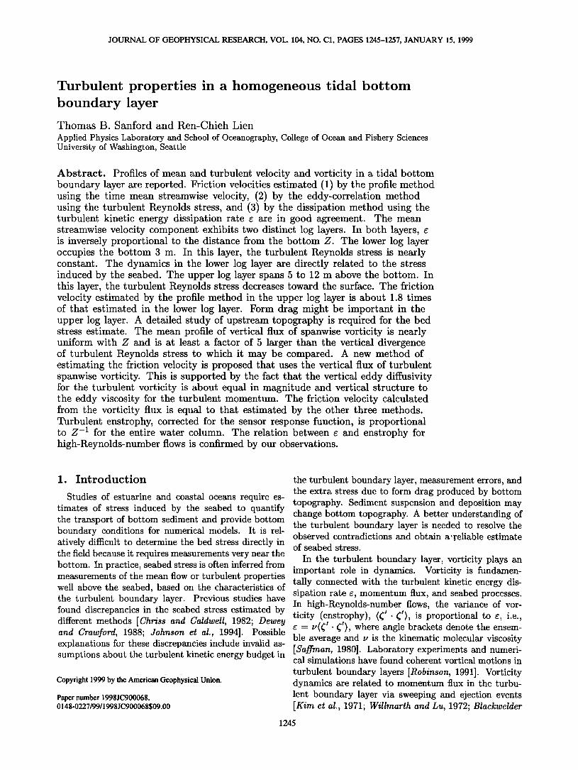
moves through a magnetic field. The EMVM sensor, electronics, pressure sensor, conductivity-temperature- depth (CTD) unit, and altimeter are installed on a tow body (Figure 1). The primary measurements of the EMVM sensor are two velocity components and one component of vorticity. Two microstructure shear probes provide measurements of •. Temperature and conductivity sensors provide measurements of temper- ature and salinity. In the latest experiment in 1997, an acoustic Doppler velocimeter (ADV) was added to provide point measurements of velocity. Velocity mea- surements taken by the ADV and the EMVM are in good agreement [Sanford et al., 1999]; they both show a spectral slope of-5/3 in the turbulence inertial sub- range. The EMVM measurements are taken at a sam- pling rate of 20 Hz, except for altitude, which is taken irregularly at a sampling rate of about 1 Hz. Attitude sensors measure motion of the EMVM vehicle, includ- ing pitch and roll as well as pitch and yaw rates. The heading of the vehicle is measured by a fluxgate com- pass mounted on the tail of the vehicle.

In this analysis, the direction of the mean horizon- tal velocity is defined as streamwise x. The orthogo- nal directions relative to the streamwise direction are

spanwise y, positive rotating clockwisely from positive x, and vertical z, positive upward. When the vorticity sensor is mounted pointing in the spanwise direction, streamwise velocity u, vertical velocity w, spanwise vor- ticity •y, and vertical strain rate OzW components are measured. Similarly, if the sensor is mounted point- ing vertically downward, streamwise velocity, spanwise velocity v, the vertical component of vorticity •z, and the spanwise strain rate OyV components are measured. In this paper, we describe observations taken while the EMVM was mounted pointing in the spanwise direction.

The four outer electrodes on the EMVM are located

0.089 m from the center electrode. The distance be-

tween the four outer electrodes and the center electrode

is defined as L. The measurements of turbulent veloc-

ity and vorticity taken from the EMVM are vertically averaged. The response functions of the observed ve- locity and vorticity spectra are calculated analytically based on the isotropic turbulent energy spectrum and the EMVM sensor configuration [Sanford et al., 1999]. The sensor response function of the vorticity spectrum shows a strong dependence on s. This dependence can be understood because the vorticity wavenumber spec- trum is nearly white, so the ratio of measured enstrophy to true enstrophy is proportional to the ratio of the tur- bulent Kolmogorov length scale (7 - /•3/4•-1/4) and the sensor scale. The response function can be adequately expressed as

(•y2)VM/(•y21true -- 2.61(•]/L) 1'23, (1) Most of our observed e values lie between 10 -5 and 10 -4 m 2 s -3. The molecular viscosity • is about 1.25 x 10 -6 m 2 s -1 for the fluid discussed here. The ratio between

SANFORD AND LIEN' TURBULENCE IN A TIDAL BOUNDARY LAYER 1247

Dissipation Electronics

Compass

CTD Sensors (T, C, P)

Altimeters

Acoustic Mirror

Tow and Data Cable

EM Velocity and Vorticity Sensors (2)

Flow Separators

Dissipation Sensors (2)

Tail Tubes

lm ! ,,

Granite Weight

I ain Electronics

Figure 1. The electromagnetic vorticity meter (EMVM) tow body. The four outer electrodes on the EMVM are located 0.089 m from the center electrode. The distance between the outer electrodes and the center electrode is defined as L. The instrument was raised and lowered to

obtain vertical profiles of properties and was occasionally held at constant depth for short periods of time. The coordinate system used in this analysis is also shown. The x axis is in the streamwise direction. During the experiment, the EMVM tow body was primarily pointing to the upstream direction. The y axis is positive out of the diagram and the z axis is positive upward.

the sensor scale and the Kolmogorov scale ranges from 135 to 240. Therefore the EMVM measures less than

1% of the true spanwise enstrophy.

2.2. Observations in a Tidal Channel

The data analyzed here were taken in Pickering Pas- sage, Washington, in a strong ebb tide during October 23-26, 1995. Pickering Passage is a 1-km-wide channel between Hartstene Island and the mainland. A multi-

beam bottom bathymetry survey was conducted in or- der to describe the bottom topography near the experi- ment site, at 47ø17.4'N 122ø53.6'W. In an earlier study, Sternberg [1968] found a well-mixed bottom boundary layer in Pickering Passage slightly south of our site. Our observation site is about 300 m upstream of a 5-m high ridge that distorts the flow. Fluctuations in the bottom topography within 1 km upstream of the experiment site are generally less than 1 m (Figure 2). Broad- crested, spanwise-oriented ripples are evident in Fig- ure 2b with 0.3-m height, 16-m wavelength, and about 100-m crest length (Figure 2c). These bed ripples are potentially important for generating the form drag (dis- cussed in' section 5.2).

The duration of the data was about 10 hours, which was split between periods when the instrument was ver- tically profiling and when it was held stationary at con- stant depths (Figure 3). Additional time was spent when the EMVM was shrouded to determine electrode

offsets. One-second averaged data are used in most of this analysis. In calculating the vorticity flux and en- strophy, 20-Hz data are used for attaining fluctuations of the small-scale turbulence because turbulent vortic-

ity is mostly at small scales. The EMVM sensor suite was mounted on a towed body, and the closest measure- ment to the bottom was about 0.45 meters above the

bottom (mab). The EMVM vehicle was usually profiled through the water column. During the profiling, the ve- hicle was usually stopped 2 m below the surface to avoid the boat's wake. The water depth, as determined from the sum of the altitude and pressure measurements, de- creases from 26 to 23 m during each of the observed ebb tidal cycles (Figure 3a). The water density de- creases during ebb tide at a rate of about 0.125 kg m -3 h -• (Figure 3b). Note that the water column is always vertically well mixed. The peak ebb tidal current ex- ceeds 0.8 m s -• near the surface (Figure 3c). Even at 0.45 mab, the tidal current is always greater than 0.2 m s -•. Vertical velocity fluctuations are O(0.1 m s -•) (Figure 3d). The slow drift of the EMVM electrode potentials results in some uncertainty in the determi- nation of absolute vorticity at a specific time, but the drift is slow enough that the vertical structure of the mean vorticity is accurately determined [Sanford et al., 1999]. Spanwise vorticity exhibits a significant vertical variation. Near the bottom, its rms value (uncorrected for the sensor response function) is about 0.5 s -• (Fig- ure 3e). The turbulent kinetic energy dissipation rate is about 10 -5 to 10 -4 m 2 s -3 near the bottom and decreases monotonically toward the water surface with a variation of at least 2 decades in the water column

(Figure 3f). There is much temporal variation in density during

the ebb tide. However, the water is nearly homogeneous over the whole water column. After the vertical mean is

1248 SANFORD AND LIEN ß TURBULENCE IN A TIDAL BOUNDARY LAYER

17.6[ (a) Observa•on Si.•te .-%.2

12- ..---• w-'7/%;-.•-_:'=:" '

17.2 gb• 17.1 .......

53.9 53.8 53.7 53.6 53.5 53.4 53.3 Lon 1 22 øW

• 100 ............................. 24

.• Observation Site •:'•'

.• 50 ........ ::::::::::::::::::::::::::::::::::::::::::::::::::::::::::::::::::::::::::::: ....... • .: .......... .•.:i::,½i: • 1.5

• 0 23 •

•: A

• -50 22.5

-100 ........... ß ................... 22 -150 -100 -50 0 50 100 150

distance east from observation site (m)

ß

23.5 rn a ' '

24 rn

-150 -100 -50 0 50 100 150 distance east from observation site (m)

Figure 2. EMVM experiment site in the center of Pick- ering Passage, Washington, and the nearby bathymetry. The bathymetry was obtained from a multibeam fath- ometer survey. (a) The large-scale bathymetry around the observation site. The direction of the ebb tidal cur-

rent is indicated. (b) Detailed bathymetry. Ripples of peak-to-peak height around 0.3 m can be identified from the image. Lines marked A and B are the vessel tracks during the survey. (c) Bathymetry from the narrow- beam fathometer survey along tracks A and B shown in Figure 2b.

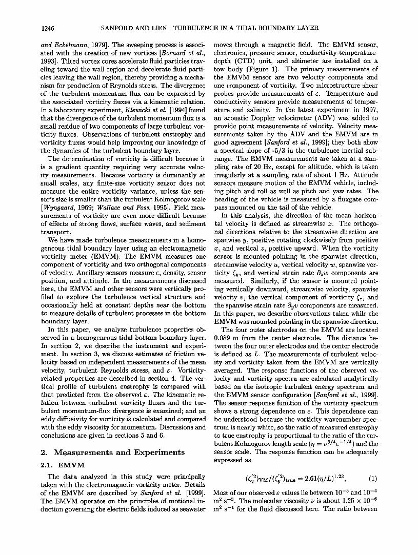
removed from each vertical profile of density, the offset density exhibits no significant vertical variation (Figure 4).

An inertial sublayer has been defined in the turbu- lent boundary layer. It lies in physical space far from the source and sink of turbulence energy. On the ba- sis of the dimensional argument [Tennekes and Lumley, 1972], the mean velocity should exhibit a logarithmic profile in the inertial sublayer, i.e.,

U- u___, In Z (2) /• z0

where • - 0.41 is von K&rm&n's constant, z0 is the bottom roughness scale, and Z is the height above the bottom. Therefore the inertial sublayer is often called the logarithmic layer (or log layer). Estimating the fric- tion velocity by fitting mean velocity measurements to (2) is called the profile method. Equation (2) is derived assuming a constant velocity scale u, in the log layer.

2 (u'w'), which requires that the By definition, u, - - turbulent Reynolds stress be constant in the log layer. Therefore the log layer is often called the constant stress layer [ Tennekes and Lumley, 1972]. Calculating the fric- tion velocity directly from turbulent Reynolds stress measurements is called the eddy-correlation method, i.e.,

- . Alternatively, the friction velocity can be estimated

from measurements of s. If a balance is assumed be-

tween s and the turbulent kinetic energy shear produc- 3/•Z, the friction tion rate, i.e., e - -(u'w•)OzU - u,

velocity can be estimated as

'•, -- (•Z)'/•. (4) This is called the dissipation method.

Sixty-three vertical profiles were taken by the EMVM as it profiled through most of the water column (see Fig- ure 3). These data will be called the profiled data in the rest of this analysis. The profiled data set is 3.6 hours long. There are about 8-9 min of data, accumulated in the 4-day period, in each vertical meter of altitude. We calculate vertical profiles of mean streamwise veloc- ity component, turbulent Reynolds stress, and turbu- lent kinetic energy dissipation rate based on the profiled data and estimate the friction velocity by three meth- ods. Data taken at fixed depths, usually lasting for 2-4 min, are used to verify the calculated vertical profiles.

3. Estimates of Friction Velocity

The seabed stress rb is related to the friction ve- locity u, - (rb/p) 1/2 where p is the water density, about 1022 4-0.0015 kg m -3. The friction velocity is often inferred from measurements of the mean velocity (profile method), the turbulent momentum flux (eddy- correlation method), or the turbulent kinetic energy dis- sipation rate (dissipation method). These methods are briefly reviewed here and then applied to our data to estimate the friction velocity.

3.1. Profile Method and Log Layer

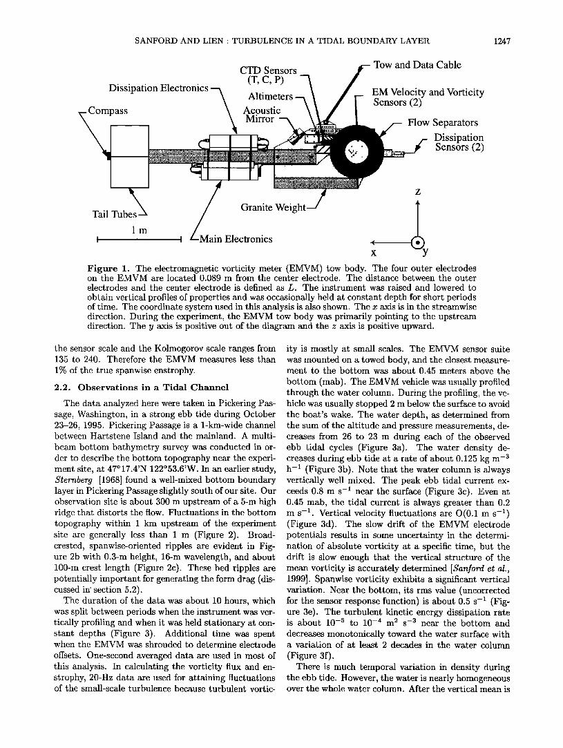
The profile method estimates the friction velocity from fits of the observed mean velocity profile to (2). Profiled data of streamwise velocity are averaged in 40 equally spaced natural logarithm depth bins (Fig- ure 5). The confidence interval of the mean velocity is calculated using the bootstrap method [Elton and Gong, 1983]. Between 4.5 mab [In(Z) : 1.5] and 12 mab [In(Z) - 2.5], there exists a well-defined log layer where the mean streamwise velocity varies linearly with

SANFORD AND LIEN- TURBULENCE IN A TIDAL BOUNDARY LAYER 1249

25 (a) 20

•lo

I

22.2 [-

22

21.9

t (b)

0.1 I () -•' 0.05

','"-"•:-","' i :"-"i" .,','" ', '"' "'"'• ,... •"""'•;"'" ','---" ',"' "",/'",'; '-' ', 0.6 (e)

,. _. t- ' I ' ' I ' I I ' I ' i '

10-• I 10 -•

10 ]8 • • • • 10/23 21:08 10/24 21'36 10/25 22:24 10/26 23:10

Figure 3. Time series of observations during the Pickering Passage experiment between October 23 and 26, 1995. The start time of observations on each day is shown at the bottom. Each tick mark interval on the abscissa is 1 hour. There are about l0 hours of data. The vehicle was mostly profiled between the surface and the bottom. Shown are (a) altitude (thin curve) and total depth (thick curve), (b) density, (c) streamwise velocity, (d) vertical velocity, (e) spanwise vorticity, and (f) turbulent kinetic energy dissipation rate. The averaged streamwise velocity between 10 and 15 meters above bottom (mab) for each profile is denoted by the thick stippled curve in Figure 3c. Note in Figure 3a that the profiler was stopped about 2 m below the surface.

In(Z). The friction velocity u,Up p estimated in this layer is up 0.043 +0.004 m s -• and the bottom roughness scale Zop

is 0.012 +0.002 m. Throughout this analysis, we will use plus/minus to represent the 95% confidence inter- val. The subscript p indicates an estimate by the profile method and the superscript "up" indicates the upper log layer. The modeled streamwise velocities based on

up up

u,p and z0p agree with the observed mean streamwise velocity in the upper log layer within 95% confidence intervals (Figure 5b). Another distinct log layer exists in the bottom 3 m, where the slope between the mean streamwise velocity and In(Z) is significantly different from that in the upper log layer. The friction velocity ulow estimated in the lower log layer is 0t024 4-0.006 m *p

1250 SANFORD AND LIEN ß TURBULENCE IN A TIDAL BOUNDARY LAYER

2O

15

10

3 times that calculated when using the friction velocity estimated in the lower log layer. A transition layer be- tween the two log layers occurs between 3 and 5 mab. The estimated bottom roughness scale _low is 2.88 times •0p the viscous scale -• low •/.•,p and reflects the height of the viscous sublayer. Using velocity measurements within 1.5 m of the bed, Sternberg [1968] estimated a friction velocity of 0.02 m s -1 and a roughness length of about 2.5 x l0 -4 m in Pickering Passage slightly south of our observational site. Our estimates of friction velocity and roughness scale in the lower log layer are consistent with Sternberg's results. We believe that the form drag plays an important dynamic role in the upper log layer and the estimated stress and roughness do not repre- sent the local bed properties. The drag coefficient and effects of ripple height on the form drag are discussed in sections 5.2 and 5.3.

0 -0.015-0.01-0.005 0 0.005 0.01

o o (kg m -•) Figure 4. Time-detrended density profiles taken in Pickering Passage. The vertical mean density of each profile has been removed in order to reveal the vertical structure (thin lines). The thick stippled line shows the 95% confidence interval of the mean density profile. See Figure 3b for the density variation before derrending.

s -1 and the bottom roughness scale _low is 1.5 + 0.2 , •0p X 10 -4 m. The superscript "low" denotes the lower log layer.

The seabed stress, rb - pu, •, calculated when using the friction velocity estimated in the upper log layer is

3.2. Eddy-Correlation Method and Constant-Stress Layer

The eddy-correlation method estimates the friction velocity from the observed turbulent Reynolds stress. Classical theory indicates that the turbulent Reynolds stress is roughly constant in the log layer and decreases linearly with distance from the boundary in the outer turbulent boundary layer. Bowden and Ferguson [1980] reported turbulent Reynolds stress,-(u•w•), which were the same at 0.5, 1, and 2 mab in a tidal boundary layer.

We calculated the turbulent Reynolds stress from the profiled data. The turbulent velocity was calculated as the difference from the vertical profile of the mean veloc- ity during each day of the 4-day experiment. Products of the fluctuating velocity components u • and w • were averaged in 1-m vertical bins to form a vertical profile

3

2.5

2

1

0.5

0

25 25

2o

510• 15 4•q 3 10

2 5

1 0

0.5 0.6 0.7 0.8 0.5 0.6 0.7 0.8

U (m s -•) U (m s -•) Figure 5. Log-layer fits to the mean streamwise velocity. The mean streamwise velocity is plotted as a function of (a) ln(Z) and (b) Z, where Z is distance from the bottom. Circles are observed mean streamwise velocity, and shading is the 95% confidence interval. The thin line indicates the log-layer fit in the upper log layer, and the thick line is the fit in the lower log layer. The log-layer fits are conducted in ln(Z) space, and the fit parameters are applied to obtain the model velocity profiles in Figure 5b. The shading at top represents the range of surface elevations during the 2-3 hours of profiling on each day.

SANFORD AND LIEN ß TURBULENCE IN A TIDAL BOUNDARY LAYER 1251

of the turbulent Reynolds stress (Figure 6). The tur- bulent stress appears to be constant in the bottom 9 m and linearly decreases to zero toward the water sur- face. The positive turbulent Reynolds stress is consis- tent with the downward transfer of positive streamwise momentum. Between 2 and 11 mab, the ratio of the 20 turbulent Reynolds stress and the observed turbulent velocity variance is about 14%; a same ratio was found by Gross and Nowell [1983].

The flux decreases to nearly zero at the sea surface, 1 • as expected for channel flows in the absence of surface • wind stress. The average Reynolds stress in the bottom • 6 m is 6 4-1 x 10 -4 m 2 s -2. On the basis of (3), the fric- [• tion velocity u,e 'is estimated to be 0.0244-0.002 m s -•, 1 0 which is consistent with the friction velocity • •ow calcu- 't•,p lated for the lower log layer. The subscript e indicates the estimate using the eddy-correlation method.

3.3. Dissipation Method and Turbulence Energy Balance

The dissipation method estimates the friction veloc- ity from measurements of • [Dewey and Crawford, 1988; 0 Johnson et al., 1994], in which a balance between • and

- <u'w'>3z U

I iiii i i i i i iiii i i i i i iiii I I i I i iiii i I i

10-7 10-6 10-s 10-4

(m 2 s -3) 25

20

15

lO

0 o 5 10

10 -4 m 2 s-2 Figure 6. Vertical profiles of turbulent momentum flux and turbulent velocity variance. Dashed line rep- resents the mean turbulent-momentum flux calculated

using data taken while the EMVM profiled through the water column, and the shading denotes its 95% confi- dence interval. Note that the Reynolds stress is zero at surface. The thick line and two thin lines are the mean

and 95% confidence intervals, respectively, for the 14% of the sum of the streamwise and vertical components of the turbulence velocity variance.

Figure 7. Vertical profiles of the turbulent kinetic en- ergy dissipation rate e and the turbulent shear produc- tion rate. The thick dashed line and shading represent the mean and the 95% confidence interval, respectively, for e. The thick line and two thin lines are the mean and 95% confidence intervals, respectively, for the turbulent kinetic energy shear production rate.

the shear production rate is assumed. Dewey and Craw- ford [1988] found that the friction velocity estimated by this method remains steady in a layer where e follows a Z -• distribution.

Two shear probes were mounted in front of the EMVM vehicle to provide independent measurements of e. The mean values of the two measurements differed by less than 10%. The mean vertical profile of e was calculated using both measurements (Figure 7). The e value de- creased away from the bottom, with a maximum value of about 4 x 10 -5 m 2 s -a.

The shear production rate, -(u•w•)OzU, was calcu- lated from estimates of the turbulent momentum flux

and the mean shear. In the bottom 10 m, the shear production rate is roughly balanced by e, so that the assumption of a local balance is appropriate. Above 10 mab the shear production rate decreases slowly ow- ing to the diminishing mean shear and is weaker than e. Note that the depth-integrated shear production rate of 1.64-0.4 x 10 -4 m a s -a agrees with the depth-integrated e, 1.4 4. 0.2 x 10 -4 m a s -a. This suggests the flow is steady and horizontal homogeneous. It is possible that a small portion of turbulent kinetic energy generated in the bottom 10 m transports upward via processes of the turbulent transport of energy or the pressure work and

1252 SANFORD AND LIEN ß TURBULENCE IN A TIDAL BOUNDARY LAYER

0.8

0.6

0.2

0 0

Figure 8.

bottom

surface

10 20 30 40

œ (10 -6 m 2 s -3)

4 5

10

25

5O

Turbulent kinetic energy dissipation rate as a function of Z -1. Circles are mean values, and shading denotes the 95% confidence interval. Thin lines represent constant friction velocity estimated as u,e - (5•Z) 1/3 .

dissipates in the upper layer. The mean shear is close to zero above 15 mab so that our estimates of shear

production vanish. The distribution of • as a function of Z -• is shown

in Figure 8. Here • is roughly proportional to Z -1 in the entire water column with large confidence intervals on estimates of • near the bottom. Following (4), the friction velocity u,e is estimated to be 0.025 -4-0.002 m s -1. The subscript • indicates the dissipation method. Therefore the friction velocity estimated by the dissipa- tion method agrees with those estimated by the profile method and eddy-correlation method. Dewey [1988] ob- served a constant • layer between 3 and 13 mab, above the constant-stress layer. Our data show no such con- stant • layer.

3.4. Comparison of Friction Velocity Estimates

Friction velocities estimated (1) by the profile method using the time mean streamwise velocity in the lower log layer, (2) by the eddy-correlation method using the turbulent Reynolds stress, and (3) by the dissipation method using the turbulent kinetic energy dissipation rate • are in good agreement, as summarized in Table 1. A new method of estimating friction velocity based on the vorticity flux also yields a similar value of friction velocity (discussed in section 4.3).

The friction velocity estimated in the upper log layer is about 1.8 times of that estimated in the lower log layer. Previous studies have also found discrepancies between the friction velocities estimated by the dis- sipation method from measurements near the bottom and by the profile method from velocity measurements above 3 mab [Dewey and Crawford, 1988; Johnson et al., 1994]. Measurements taken from bottom-mounted tripods provide details of turbulent and mean-flow prop- erties near the bottom boundary layer but do not de- scribe the upper portion of the flow [Trowbridge et al., 1996]. On the other hand, bottom-mounted acoustic Doppler current profilers (ADCPs) measure spatial and temporal variations of the mean flow in the upper por- tion of the flow but do not measure the flow near the

bottom few meters because of the size of the ADCP and

the blanking distance required for ADCP measurements [Lueck and Lu, 1997]. An advantage of the present method is its ability to profile more of the water column to describe the dynamics of both log layers adequately.

4. Vorticity Properties in the Boundary Layer

4.1. Enstrophy

In a tidal boundary layer, the primary vorticity com- ponent is in the spanwise direction as shown by Viek- man et al. [1989]. Streamwise and vertical vorticity components arise because of the lift of the spanwise vorticity. These vortical motions have been observed in laboratory experiments and are described in detail by Robinson [1991]. In high-Reynolds-number flows, en-

Table 1. Summary of Friction Velocity Estimates

Methods Friction Velocity u,, m s -• Depth Range, meters above bottom

Profile method, upper log layer Profile method, lower log layer Eddy-correlation method Dissipation method Vorticity-fiux method

0.043 4- 0.004 up (u,p ) 5 - 12 0.024 4- 0.006 ' low, [U,p ) 0.5 - 3 0.024 q- 0.002 (u,e) 0.5- 6 0.025 4- 0.002 (u,•) 0.5- 10 o.o2s + o.oos o.s-

Subscripts denote p, profile method; e, eddy-correlation method; •, dissipa- tion; and (, vorticity-fiux method. Superscripts "up" and "low" represent upper and lower layer, respectively.

SANFORD AND LIEN ß TURBULENCE IN A TIDAL BOUNDARY LAYER 1253

strophy is directly related to the turbulent kinetic en- ergy dissipation rate [Tennekes and Lumley, 1972], i.e., e - •(•'-•'/, where (•'-•') is the total enstrophy, the sum of three components.

The EMVM sensor measures the spanwise component of enstrophy at scales greater than the sensor scale of 0.089 m. The observed spanwise enstrophy and tur- bulent kinetic energy dissipation rate are significantly correlated with a correlation coefficient of 0.27 and a

95% significance level of 0.018. The measured spanwise enstrophy is corrected for the sensor response based on (1). In a laboratory experiment, Balint et al. [1991] found that enstrophy decreased away from the bound- ary as Z -1. Our corrected enstrophy was inversely pro- portional to the distance from the bottom (Figure 9). It was approximately equal to 9 Z -1 (s-:) for most of the water column. It agrees with the vertical distri- bution of e/3•. Therefore the relation • - 3•(•'y e) for high-Reynolds-number flows is confirmed by our data.

the momentum flux is related to the creation of new

vortices at the boundary [Bernard et al., 1993]. There is a kinematic relation between the turbulent

vorticity flux and the divergence of the turbulent mo- mentum flux [Klewicki et al., 1994], i.e.,

OXj ---- --•ijk(tt'J•l -•- • 0X i ' (5) where the tensor notation and the summation conven-

tion with respect to repeated indices are used and eijk is the alternating, third-order tensor.

Using data from laboratory experiments, Klewicki et al. [1994] examined the streamwise component of (5), i.e.,

O(u'w') O(u'v') 10(u'u'- v'v' - w'w') + +-

Oz Oy 2 Ox

= (6)

4.2. Vorticity Flux

Laboratory experiments and numerical simulations of boundary layer turbulence have shown coherent vortical motions in turbulent boundary layers [Robinson, 1991]. These vortical motions play an important role in the momentum transfer between inner and outer boundary layers [Kim et al., 1971; Willmarth and Lu, 1972; Black- welder and Eckelmann, 1979]. The sweeping process of

1

0.8

0.6 0.4

0.2

0 0 5 10

(s -2)

Figure 9. Vertical profiles of the spanwise enstrophy corrected for the sensor response (1). Circles and shad- ing are the mean and 95% confidence interval, respec- tively, of the corrected spanwise vorticity. The thick solid line is the mean of e/3• based on observed e, and the two thin solid lines are the 95% confidence intervals.

The dashed line represents (•'y2)corrected -- 9Z-1(s-2), '2

which is an approximate form of observed ((v )corrected.

The second term is generally much smaller than the first term because the length scale in the spanwise di- rection is greater than that in the vertical direction, i.e., a small aspect ratio. The third term is unrelated to the turbulent vorticity flux and is called the inactive component of the momentum-flux divergence [Turner, 1973]. The two terms on the right-hand side of (6) are associated with vorticity fluxes and are called the active component of the turbulent momentum-flux divergence. The inactive component is at least 1 order of magni- tude smaller than the active components [Klewicki et al., 1994]. Therefore (6) can be simplified as

t t

= <w'•y> -<V'•z >. (7) Oz

Klewicki et al. [1994] found that both the vertical flux of the spanwise vorticity (w'•}> and the spanwise flux of the vertical vorticity <v'•> contribute to the momentum-flux divergence. The spanwise flux of the vertical vorticity is associated with the vortex-stretching force of the primary spanwise vorticity and therefore is related to the change of turbulence scales [ Termekes and Lumley, 1972]. In turbulent jets and wakes, the turbu- lence scale is roughly constant in the cross-stream di- rection, so the spanwise flux of the vertical vorticity can be neglected. In the turbulent boundary layer, however, the turbulence scale increases away from the boundary, and <w'•) and <v'•'z) are of similar magnitude.

The EMVM measurements provide estimates of the vertical divergence of the turbulent momentum flux and the vertical flux of the spanwise vorticity, the first two terms in (7). The vertical profile of the vorticity flux was calculated using the profiled data. In every 1-m vertical bin, the turbulent vorticity and vertical veloc- ity were calculated by removing their mean values for each of the 4 days. The product of the turbulent verti- cal velocity and spanwise vorticity was averaged in 1-m depth bins for each day and then averaged over the 4-

1254 SANFORD AND LIEN ß TURBULENCE IN A TIDAL BOUNDARY LAYER

25

2O

15

l0

i i i i i 0 2 4 6

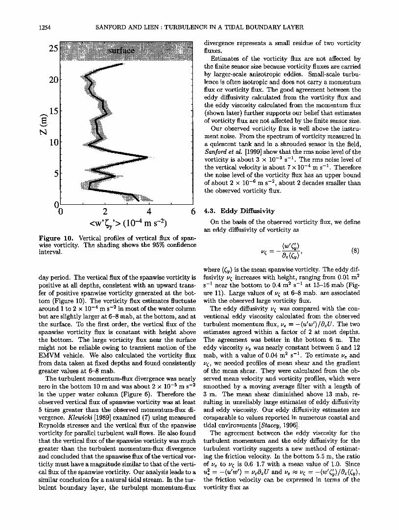
<w' > (10 -4 m s -2) Figure 10. Vertical profiles of vertical flux of span- wise vorticity. The shading shows the 95% confidence interval.

divergence represents a small residue of two vorticity fluxes.

Estimates of the vorticity flux are not affected by the finite sensor size because vorticity fluxes are carried by larger-scale anisotropic eddies. Small-scale turbu- lence is often isotropic and does not carry a momentum flux or vorticity flux. The good agreement between the eddy diffusivity calculated from the vorticity flux and the eddy viscosity calculated from the momentum flux (shown later) further supports our belief that estimates of vorticity flux are not affected by the finite sensor size.

Our observed vorticity flux is well above the instru- ment noise. From the spectrum of vorticity measured in a quiescent tank and in a shrouded sensor in the field, Sanford et al. [1999] show that the rms noise level of the vorticity is about 3 x 10 -3 s -t. The rms noise level of the vertical velocity is about 7 x 10 -4 m s -t. Therefore the noise level of the vorticity flux has an upper bound of about 2 x 10 -6 m s -2 about 2 decades smaller than

the observed vorticity flux.

4.3. Eddy Diffusivity

On the basis of the observed vorticity flux, we define an eddy diffusivity of vorticity as

=

day period. The vertical flux of the spanwise vorticity is positive at all depths, consistent with an upward trans- fer of positive spanwise vorticity generated at the bot- tom (Figure t0). The vorticity flux estimates fluctuate around t to 2 x 10 -4 m s -2 in most of the water column

but are slightly larger at 6-8 mab, at the bottom, and at the surface. To the first order, the vertical flux of the spanwise vorticity flux is constant with height above the bottom. The large vorticity flux near the surface might not be reliable owing to transient motion of the EMVM vehicle. We also calculated the vorticity flux from data taken at fixed depths and found consistently greater values at 6-8 mab.

The turbulent momentum-flux divergence was nearly zero in the bottom t0 m and was about 2 x 10 -5 m s -2

in the upper water column (Figure 6). Therefore the observed vertical flux of spanwise vorticity was at least 5 times greater than the observed momentum-flux di- vergence. Klewicki [1989] examined (7) using measured Reynolds stresses and the vertical flux of the spanwise vorticity for parallel turbulent wall flows. He also found that the vertical flux of the spanwise vorticity was much greater than the turbulent momentum-flux divergence and concluded that the spanwise flux of the vertical vor- ticity must have a magnitude similar to that of the verti- cal flux of the spanwise vorticity. Our analysis leads to a similar conclusion for a natural tidal stream. In the tur-

bulent boundary layer, the turbulept momentum-flux

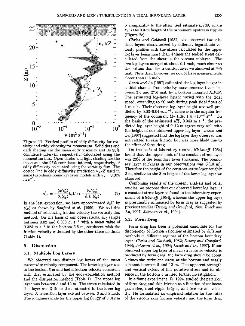
where <•y/is the mean spanwise vorticity. The eddy dif- fusivity •½ increases with height, ranging from 0.01 m 2 s -• near the bottom to 0.4 m e s -• at 15-16 mab (Fig- ure 11). Large values of •½ at 6-8 mab. are associated with the observed large vorticity flux.

The eddy diffusivity v½ was compared with the con- ventional eddy viscosity calculated from the observed turbulent mornentum flux, •e - -<u•w•l/OzU. The two estimates agreed within a factor of 2 at most depths. The agreement was better in the bottom 6 m. The eddy viscosity •e was nearly constant between 5 and 12 mab, with a value of 0.04 m e s -t. To estimate •e and •½, we needed profiles of mean shear and the gradient of the mean shear. They were calculated from the ob- served mean velocity and vorticity profiles, which were smoothed by a moving average filter with a length of 3 m. The mean shear diminished above 13 mab, re- sulting in unreliably large estimates of eddy diffusivity and eddy viscosity. Our eddy diffusivity estimates are comparable to values reported in numerous coastal and tidal environments [Stacey, 1996].

The agreement between the eddy viscosity for the turbulent momentum and the eddy diffusivity for the turbulent vorticity suggests a new method of estimat- ing the friction velocity. In the bottom 5.5 m, the ratio of •e to •½ is 0.6-1.7 with a mean value of t.0. Since 2 _(u•w •) •'ec9zU and •'e • •'½ -(w•y)/C9z(•y),

the friction velocity can be expressed in terms of the vorticity flux as

SANFORD AND LIEN ß TURBULENCE IN A TIDAL BOUNDARY LAYER 1255

25

2O

15

l0

Figure 11. Vertical profiles of eddy diffusivity for vor- ticity and eddy viscosity for momentum. Solid dots and dark shading are the mean eddy viscosity and its 95% confidence interval, respectively, calculated using the momentum flux. Open circles and light shading are the mean and the 95% confidence interval, respectively, of eddy diffusivity calculated using the vorticity flux. The dotted line is eddy diffusivity prediction u, nZ used in some turbulence boundary layer models with u, - 0.024

--1 ms .

In the last expression, we have approximated OzU by ((y) as shown by Sanford et al. [1999]. We call this method of calculating friction velocity the vorticity flux method. On the basis of our observations, u,C ranges between 0.02 and 0.033 m s -1 with a mean value of 0.025 m s -1 in the bottom 5.5 m, consistent with the friction velocity estimated by •he other •hree methods (Table 1).

5. Discussion

5.1. Multiple Log Layers

We observed two distinct log layers of the mean streamwise velocity component. The lower log layer was in the bottom 3 m and had a friction velocity consistent with that estimated by the eddy-correlation method and the dissipation method (Table 1). The upper log layer was between 5 and 12 m. The stress calculated in this layer was 3 times that estimated in the lower log layer. A transition layer existed between 3 and 5 mab.

up of 0.012 m The roughness scale for the upper log fit Zov

is comparable to the often used estimate ks/30, where ks is the 0.3-m height of the prominent upstream ripples (Figure 2c).

Chriss and Caldwell [1982] also observed two dis- tinct layers characterized by different logarithmic ve- locity profiles with the stress calculated for the upper log layer being more than 4 times the seabed stress cal- culated from the shear in the viscous sublayer. The two log layers merged at about 0.1 mab, much closer to the bottom than the transition layer we observed at 3-5 mab. Note that, however, we do not have measurements closer than 0.5 mab.

Lueck and Lu [1997] estimated the log-layer height in a tidal channel from velocity measurements taken be- tween 3.6 and 27.6 mab by a bottom mounted ADCP. The estimated log-layer height varied with the tidal speed, extending to 20 mab during peak tidal flows of I rn s -1. Their observed log-layer height was well pre- dicted by 0.03-0.04 u,w -1, where w is the angular fre- quency of the dominant Ms tide, 1.4 x10 -4 s -1. On the basis of the estimated up s_1 U,p, 0.043 m , the pre- dicted log-layer height of 9-12 m agrees very well with the height of our observed upper log layer. Lueck and Lu [1997] suggested that the log layer they observed was not related to skin friction but was more likely due to the effect of form drag.

On the basis of laboratory results, Klebanoff [1954] found that the upper limit of the constant-stress layer was 20% of the boundary layer thickness. The bound- ary layer thickness in our observations was O(10 m). Therefore the height of the constant-stress layer roughly 2 m, similar to the 3-m height of the lower log layer we observed.

Combining results of the present analysis and other studies, we propose that our observed lower log layer is a constant stress layer as found in the laboratory exper- iment of Klebanoff [1954], whereas the upper log layer is presumably influenced by form. drag as suggested by previous studies [Dewey and Crawford, 1988; Lueck and Lu, 1997; Johnson et al., 1994].

5.2. Form Drag

Form drag has been a potential candidate for the discrepancy of friction velocities estimated by different methods in different regimes of the bottom boundary layer [Chriss and Caldwell, 1982; Dewey and Crawford, 1988; Johnson et al., 1994; Lueck and Lu, 1997]. If our observed upper log layer of mean streamwise velocity is produced by form drag, the form drag should be about 3 times the turbulent stress at the bottom and nearly constant between 5 and 12 m. The apparent strength and vertical extent of this putative stress and its ab- sence in the bottom 5 m need further investigation.

In a flume experiment, Li [1994] studied the partition of form drag and skin friction as a function of sediment grain size, sand ripple height, and free stream veloc- ity. He formulated an empirical relation for the ratio of the viscous skin friction velocity and the form drag

1256 SANFORD AND LIEN ß TURBULENCE IN A TIDAL BOUNDARY LAYER

shear friction velocity as a function of the flow param- eter u.d -• , where u. is the total shear friction velocity and d is the sand ripple height. Our analysis suggests that the total friction velocity is 0.043 m s -• and the viscous skin friction velocity is 0.024 m s -• . Following Li's [1994] formula, the ripple height is estimated to be about 0.01-0.02 m. Interestingly, it has the same scale

up the roughness scale in the upper log layer. as ZOp •

5.3. Drag Coei•cient

Seabed stress is frequently calculated from near-bed velocity measurements by assuming a drag coefficient C•00 defined as

2

u, _ n (10) Coo = Uoo - pUoo' where Uxoo is the mean velocity at I mab Sternberg [1968] found C•oo was 2.3 x 10 -8 for measurements taken in Pickering Passage slightly south of our site. Our mean velocity at I mab is 0.54 m s -•, and the friction velocity - •ow - 0.024 + 0.006 m s -• '•,p • •-/,e ß Therefore the drag coefficient at our site is 2.0 + 0.6 x 10 -•, in reasonable agreement with Sternberg's value. The 95% confidence interval is based on the average of the confidence intervals of - •ow and U,e ß C•,p .

6. Summary and Conclusion

We have analyzed measurements taken within a ho- mogeneous, fully developed turbulent bottom boundary layer. The main themes of this study are (1) estimating friction velocity based on three conventional methods using simultaneous, independent measurements, and (2) estimating the turbulent vorticity flux and enstro- phy in the bottom boundary layer (we propose a new method of calculating friction velocity based on the vor- ticity flux).

The friction velocities estimated from our data when

using the profile, eddy-correlation, and dissipation meth- ods agree with each other within their 95% confidence intervals (Table 1). The near-bottom profile method found that the friction- velocity is 0.024 m s -•, and the bottom roughness scale is 1.5 x 10 -4 m. These values are consistent with the results of a previous study by Sternberg [1968] that used measurements taken near our experiment site.

We found two distinct log layers of mean streamwise velocity separated by a transition layer between 3 and 5 mab. The lower log layer extends from the bottom to about 3 mab, and the upper log layer is between 5 and 12 mab. The calculated friction velocity in the upper log layer is about 1.8 times of that in the lower log layer. This might explain discrepancies observed between fric- tion velocities estimated bY the dissipation method from near-bottom measurements and by the profile method from upper layer mean velocity measurements [Johnson et al., 1994; Dewey and Crawford, 1988]. The higher

stress in the upper log layer could be due to the form drag.

The vertical profile of turbulent Reynolds stress also exhibits two different regions. The turbulent Reynolds stress shows no significant vertical variation within 9 mab and decreases linearly toward the water surface above 9 mab. The separation of these two regions, the bottom constant-stress region and the upper linear- decay region, is not as clear as that between the two log layers, primarily because the large confidence inter- val for the estimated Reynolds stress. Nevertheless, it is clear that the constant-stress layer does not extend beyond 10 mab.

In the bottom 10 m, there is a balance between the turbulent kinetic energy shear production rate and vis- cous dissipation rate. The turbulent kinetic energy dis- sipation rate is inversely proportional to the distance from the bottom. The observed enstrophy profile agrees with that predicted from the observed e. After cor- rection for the sensor response function, enstrophy is inversely proportional to the distance from the bound- ary. The relation • - 3•(•'y•/for high-Reynolds-number flows is also confirmed.

We report the first field observations of the covari- ance between the components of vertical velocity and spanwise vorticity. The results confirm the expected upward flux of spanwise vorticity from the source at the bottom. The flux is uniform with the height above the bottom, suggesting a sink near the surface, closer to the surface than our observations (usually 2 m below the surface), or a sink further downstream, in violation of the assumed lack of downstream gradient. Additional vorticity measurements are needed within 2 m of the surface in future experiments.

We examined the kinematic relation between turbu-

lent momentum-flux divergence and vorticity flux. The observed vertical flux of the spanwise vorticity is almost I order of magnitude greater than the vertical gradient of the momentum flux, suggesting that the unmeasured spanwise flux of the vertical vorticity is of the same order of magnitude as the observed vertical flux of the spanwise vorticity. This is consistent with Tennekes and Lumley's [1972] theoretical arguments and Klewicki et al's [1994] observations.

The eddy diffusivity for turbulent vorticity has a mag- nitude and vertical structure similar to those of the

eddy viscosity for turbulent momentum. On the basis of this result, we propose a new method of estimating the friction velocity that uses the turbulent vorticity flux. The new vorticity flux method yields a friction velocity in good agreement with conventional methods. This method may have advantages for field observations where velocity from irrotational surface gravity waves complicates alternative methods.

We think the height where the log fits change (i.e., 3-5 mab) and the ratio of upper to lower stress are related to upstream bedform. Perhaps, the two log lay- ers are a direct result of the prominent roughness just

SANFORD AND LIEN: TURBULENCE IN A TIDAL BOUNDARY LAYER 1257

upstream of the observations (Figure 2). It is evident from Figure 2 that bottom roughness is not uniform upstream. As a result, turbulent properties at a given height may result in response to upstream roughness rather than the roughness directly beneath the sen- sor. The transition should be closer to the bottom for

smoother bottom roughness. Our results suggest that detailed bathymetry should be measured around any site where bottom boundary layer turbulence is studied. Future studies will attempt to quantify the influences of the distribution of upstream bottom roughness.

We are analyzing data taken in later experiments in Pickering Passage to study the effect of stratification on the turbulent boundary layer. The kinematic relation between the turbulent momentum-flux divergence and vorticity flux will be revisited with additional measure- ments of the spanwise flux of the vertical vorticity.

Acknowledgments. We are grateful to James Carlson, who exhibited great skill in the design and construction of the EMVM and its suite of sensors. Gordon Welsh designed the EMVM vehicle. Mark Prater devoted much effort on

making an early version of the EMVM work. John Dunlap developed the data acquisition system and processed data. His efforts in processing dissipation measurements are es- pecially appreciated. The observations were made with the vital help of James Carlson, John Dunlap, and Eric Boget under occasionally dii•cult conditions. Scientific advice was provided by Eric D'Asaro, Eric Kunze, and Harvey Seim. This research was supported by the Oi•ce of Naval Research.

References

Balint, J.-L., J. M. Wallace, and P. Vukoslavcevic, The ve- locity and vorticity vector fields of a turbulent boundary layer, 2, Statistical properties, J. Fluid Mech., 228, 53-86, 1991.

Bernard, P.S., J. M. Thomas, and R. A. Handler, Vortex dynamics and the production of Reynolds stress, J. Fluid Mech., 253, 385-419, 1993.

Blackwelder, R. F., and H. Eckelmann, Streamwise vortices associated with the bursting phenomenon, J. Fluid Mech., 9J, 557-594, 1979.

Bowden, K. F., and S. R. Ferguson, Variation with height of the turbulence in a tidally-induced bottom boundary layer, in Marine Turbulence, edited by J. Nihoul, pp. 258- 286, Elsevier Sci., New York, 1980.

Chriss, T. M., and D. R. Caldwell, Evidence for the influence of form drag on bottom boundary layer flow, J. Geophys. Res., 87, 4148-4154, 1982.

Dewey, R. K., The constant production-dissipation rate layer of the oceanic bottom boundary layer, paper pre- sented at Eighth Symposium on Turbulence and Diffu- sion, Am. Meterol. Soc., San Diego, Calif., April 26-29, 1988.

Dewey, R. K., and W. R. Crawford, Bottom stress estimates from vertical dissipation rate profiles on the continental shelf, J. Phys. Oceanogr., 18, 1167-1177, 1988.

Efron, B., and G. Gong, A leisurely look at the bootstrap, jackknife and cross-validation, Am. Statist., 37, 36-48, 1983.

Gross, T. F., and A. R. M. Nowell, Mean flow and turbulence scaling in a tidal boundary layer, Cont. Shelf Res., 2, 109- 126, 1983.

Johnson, G. C., R. G. Lueck, and T. B. Sanford, Stress on the Mediterranean Outflow plume, 2, Turbulent dissi- pation and shear measurements, J. Phys. Oceanogr., 2•, 2084-2092, 1994.

Kim, H. T., S. J. Kline, and W. C. Reynolds, The production of turbulence near a smooth wall in a turbulent boundary layer, J. Fluid Mech., 50, 133-160, 1971.

Klebanoff, P., Characteristics of turbulence in a boundary layer with zero pressure gradient, Natl. Advisory Comm. Aeronaut., Publ. NA CA TN 3178, 1954.

Klewicki, J. C., Velocity-vorticity correlations related to the gradients of the Reynolds stresses in parallel turbulent wall flows, Phys. Fluids, A, 1, 1285-1288, 1989.

Klewicki, J. C., J. A. Murray, and R. E. Falco, Vortical mo- tion contributions to stress transport in turbulent bound- ary layers, Phys. Fluids, 6, 277-286, 1994.

Li, M. Z., Direct skin friction measurements and stress par- titioning over movable sand ripples, J. Geophys. Res., 99, 791-799, 1994.

Lueck, R. G., and Y. Lu, The logarithmic layer in a tidal channel, Cont. Shelf Res., 17, 1785-1861, 1997.

Robinson, S. K., Coherent motions in the turbulent bound- ary layer, Annu. Rev. Fluid Mech., 23, 601-639, 1991.

Saffman, P. G., Vortex interactions and coherent structures in turbulence, in Transition and Turbulence, edited by R. E. Meyer, Univ. of Wis. Press, Madison, 1980.

Sanford, T. B., J. A. Carlson, J. H. Dunlap, M.D. Prater, and R.-C. Lien, An electromagnetic vorticity and velocity sensor for observing finescale kinetic fluctuations in the ocean, J. Atmos. Oceanic Technol., in press, 1999.

Stacey, M. T., Turbulent mixing and residual circulation in a partially stratified estuary, Ph.D. dissertation, 209 pp., Stanford Univ., Stanford, Calif., 1996.

Sternberg, R. W., Friction factors in tidal channels with differing bed roughness, Mar. Geol., 6, 243-260, 1968.

Tennekes, H., and J. L. Lumley, A First Course in Turbu- lence, 300 pp., MIT Press, Cambridge, Mass., 1972.

Trowbridge, J. H., A. J. Williams and W. J. Shaw, Measure- ments of Reynolds stress and heat flux with an acoustic travel-time current meter, paper presented at a Workshop on Microstructure Sensors in the Ocean, Off. Naval Res., Timberline, Oreg., Oct. 23-25, 1996.

Turner, J. S., Buoyancy Effects in Fluids, 367 pp., Cam- bridge Univ. Press, New York, 1973.

Viekman, B. E., M. Wirebush, and J. C. Van Leer, Sec- ondary circulations in the bottom boundary layer over sedimentary furrows, J. Geophys. Res., 9•, 9721-9730, 1989.

Wallace, J. M., and J. F. Foss, The measurement of vorticity turbulent flows, Annu. Rev. Fluid Mech., 27, 469-514, 1995.

Willmarth, W. W., and S. S.'Lu, Structure of the Reynolds stress near the wall, J. Fluid Mech., 55, 65-92, 1972.

Wyngaard, J.C., Spatial resolution of the vorticity meter and other hot-wire arrays, J. Sci. Instrum., 2, 9983-9987, 1969.

R.-C. Lien and T. B. Sanford, Applied Physics Lab- oratory and School of Oceanography, College of Ocean and Fishery Sciences, University of Washington, Seat- tle, Washington 98105. (lien@apl.•vashington.edu; san- ford @ap 1. washington.edu)

(Received April 21, 1998; revised September 11, 1998; accepted October 15, 1998.)