Turbulence intensity calculation using Gaussian Processes on ...

TNO PUBLIC

TNO PUBLIC

Westerduinweg 3

1755 LE Petten

P.O. Box 15

1755 ZG Petten

The Netherlands

www.tno.nl

T +31 88 866 50 65

TNO report

TNO2021 R11603 | Final report

Turbulence intensity calculation using

Gaussian Processes on the wind speeds

measured by nacelle mounted lidar

Date 15 October 2021

Author(s) C. Liu; E.J. Rose

Copy no

No. of copies

Number of pages 19 (incl. appendices)

Number of

appendices

Sponsor RVO - TKI Wind op Zee HER

Project name GE Haliade X Demonstration: Innovations in Type Certificaiton

Project number 060.34375

All rights reserved.

No part of this publication may be reproduced and/or published by print, photoprint,

microfilm or any other means without the previous written consent of TNO.

In case this report was drafted on instructions, the rights and obligations of contracting parties

are subject to either the General Terms and Conditions for commissions to TNO, or the

relevant agreement concluded between the contracting parties. Submitting the report for

inspection to parties who have a direct interest is permitted.

© 2021 TNO

TNO PUBLIC

draft

TNO PUBLIC | TNO report | TNO2021 R11603 | Final report 2 / 19

Summary

Wind measurement is probably the most essential input for any wind energy

technology applications. The wind speed and turbulence intensity are traditionally

and still popularly measured with cup anemometer or sonic anemometer.

In recent years lidar technology, and particularly nacelle lidar technology, emerged

in the wind energy industry with its many advantages: reduced cost compared to

meteorological mast; always measuring in front of the wind turbine to enable a wider

measurement sector with high correlation to wind power; measuring at more ranges;

measuring over a plane or volume instead of a point; potability; assisting smart wind

turbine control etc. It is adopted by the industry through various pilot and commercial

projects over the world for warranty Power Performance Testing already. The IEC

standards based on the best practices for ground based lidar, nacelle mounted lidar

and floating lidar are coming on their way. However lidar is still not accepted for

turbulence measurements.

A novel application of Machine Learning for lidar measurement was developed by

TNO Wind Energy, based on Gaussian Process regression, to produce reconstructed

wind field from lidar measurements. In this report, the potentials of using Gaussian

Process regression to improve the wind turbulence intensity for lidar wind

measurements are studied with several Gaussian Process implementation tests:

upsampling the data to higher frequency, filling missing data, predicting in space and

predicting in the center of the beams. For a two-beam lidar, although the Gaussian

Process does not show effective improvements for calculating turbulence intensity.

The main reasons are firstly that its bias towards the mean values when predicting

away from measurement data, and secondly that it relies on the methods of

converting the radial wind speeds to horizontal wind speeds. However the results do

demonstrate that Gaussian Process can be applied to almost any lidar system to

predict beam radial wind speeds in space and time. And there is still potential to

improve turbulence intensity by using lidar with more beams for predictions within a

volume as opposed to a plane, or by further developing Gaussian Process

mechanisms to calculate turbulence intensity with different methods.

TNO acknowledges Leosphere for using their lidar data in this project.

TNO PUBLIC


Contents

Summary .................................................................................................................. 2

1 Introduction .............................................................................................................. 4

2 Technical Background ............................................................................................ 5 2.1 Wind turbine Type Certification (TC) ......................................................................... 5 2.2 Lidar ........................................................................................................................... 5 2.3 Gaussian Process (GP) ............................................................................................. 6

3 Turbulence Intensity calculation ........................................................................... 8 3.1 Wind dataset .............................................................................................................. 8 3.2 Wind field reconstruction ......................................................................................... 10 3.3 GP implementation .................................................................................................. 11 3.4 Results ..................................................................................................................... 11

4 Conclusions ........................................................................................................... 18

5 References ............................................................................................................. 19

TNO PUBLIC


1 Introduction

Wind measurement is probably the most top essential input for any wind energy

technology applications. The wind speed and turbulence intensity (TI) are traditionally

and still popularly measured with cup anemometer or sonic anemometer.

In recent years the lidar (Light Detection and Ranging) technology, and particularly

nacelle lidar technology, emerged in the wind energy industry with its many

advantages: reduced cost compared to meteorological mast (MM); always measuring

in front of the wind turbine to enable a wider measurement sector with high correlation

to wind power; measuring at more ranges; measuring over a plane or volume instead

of a point; potability; assisting smart wind turbine control etc. It is adopted by the

industry through various pilot and commercial projects over the world for Power

Performance Testing already. The IEC standards based on the current best practices

for ground based lidar, nacelle mounted lidar and floating lidar are coming on their

way. However lidar is still not accepted for turbulence measurements [1].

A novel application of Machine Learning (ML) for lidar measurement was developed

by TNO Wind Energy [4], based on Gaussian Process (GP) regression, to produce

reconstructed wind fields from lidar measurements. In this report, the potential of

using GP regression to improve the wind TI calculation for lidar wind measurements

are studied and the results are presented.

Chapter 2 describes the technical background about wind turbine Type Certification

(TC), lidar and GP. Chapter 3 describes the wind field reconstruction using GP and

results from different implementations tests. Chapter 4 gives the conclusions and

recommendations for future work.

TNO PUBLIC


2 Technical Background

2.1 Wind turbine Type Certification (TC)

Wind turbine TC is a must-have for wind turbine OEMs to be able to bring their

products to market. The type certification process provides confirmation that the wind

turbine type, components and systems have been designed, manufactured and

tested in conformity with the requirements as mandated by international standards

and site-specific condition. It is an all-inclusive verification of wind turbine safety,

reliability and performance according to standards, which makes it quite a time

consuming process. Moreover with the increase of wind turbine size, the time of the

type certification process is also increasing.

Type testing evaluation is part of the type certification, where a prototype is erected

and tested on site. During type testing, the wind properties need to be measured.

Following the latest IEC standard [2], a remote sensing device (RSD) can be

deployed, but this is limited to non-complex terrain and a short MM (not less than the

minimum of the wind turbine lower blade tip-height or 40m) must exist for comparison

purpose.

Lidar has been in the spotlight of IEC standardisation over the recent years. It is not

only because of its high potentials to bring down both the time and cost of wind

measurement, but also because of the innovative applications of lidar which can

reduce the Cost of Energy (CoE) effectively such as yaw misalignment correction,

site suitability pre-construction studies and lidar assisted control etc. The draft IEC

guideline IEC 61400-50-2 for application of ground based lidar (GBL) and the draft

IEC guideline IEC 61400-50-3 for application of nacelle mounted lidar (NML) are

submitted to all IEC members in 2021 and on the way to the final release. The IEC

guideline IEC 61400-50-4 for application of floating lidar will also come as planned in

2022. It will be a big step to have all those IEC standards to speed up the application

of lidar for TC, however there are still many research challenges for further

applications of lidar, such as the application in complex terrain or superseding MM

completely.

2.2 Lidar

Lidar is based on Doppler shift of the backscattered light to determine the wind speed

in the line of sight (LOS) direction.

There are different types of lidar. Most commercial wind lidars use homodyne

detection to determine the Doppler shift. With homodyne detection information on the

magnitude of the shift is gathered, but no information on whether it is positive or

negative which means the wind is towards the lidar or away from the lidar is unknown.

The heterodyne detection gathers both magnitude and sign but requires more

hardware which drives up the cost to produce a lidar. Another way to categorize the

lidar is based on it is light source: pulsed wave or continuous wave. For pulsed lidar,

the time of the pulsed light used to travel to the target and back is used to determine

the measurement distance. For continuous wave lidar, the measurement distance is

determined by focus. According to the application, the lidar is also commonly

categorized as GBL, NML, scanning lidar and floating lidar.

TNO PUBLIC


The application of different lidar technology in wind energy industry had been

researched for many years. TNO Wind Energy (formerly known as ECN Wind

Energy) also conducted a large test campaign to study and quantify numerous

advantages of GBL, NML and scanning lidar [3].

Nowadays lidar is accepted and used for warranty Power Performance Testing

(PPT). However for TC, an installed lidar without accompanying MM is still not

accepted in the latest IEC standard [2] to provide wind measurements for power

performance and mechanical loads measurements. One of the possible reasons is

that current lidar technology obtains TI measurements differently than a wind cup

anemometer or sonic anemometer mounted on a MM.

Lidar technologies perform averaging over a large measurement volume (i.e. the

probe volume). For turbulence measurements, this has a similar effect as applying a

low pass filter, which reduces the standard deviation of the measured signal (i.e. wind

velocities) resulting in reduced values of the TI. Deducing unfiltered turbulence

statistics from the raw lidar data has been and remains the most challenging aspect

of lidar application and many research has been done to develop algorithms to

improve this situation [1].

Another drawback of lidar technology is that using a single lidar with only LOS wind

speeds makes it impossible to distinguish between wind shear and wind direction.

This is called the cyclops dilemma (ref?). Currently the standard wind field

reconstruction algorithms from lidar manufacturers assume homogeneous wind flow.

2.3 Gaussian Process (GP)

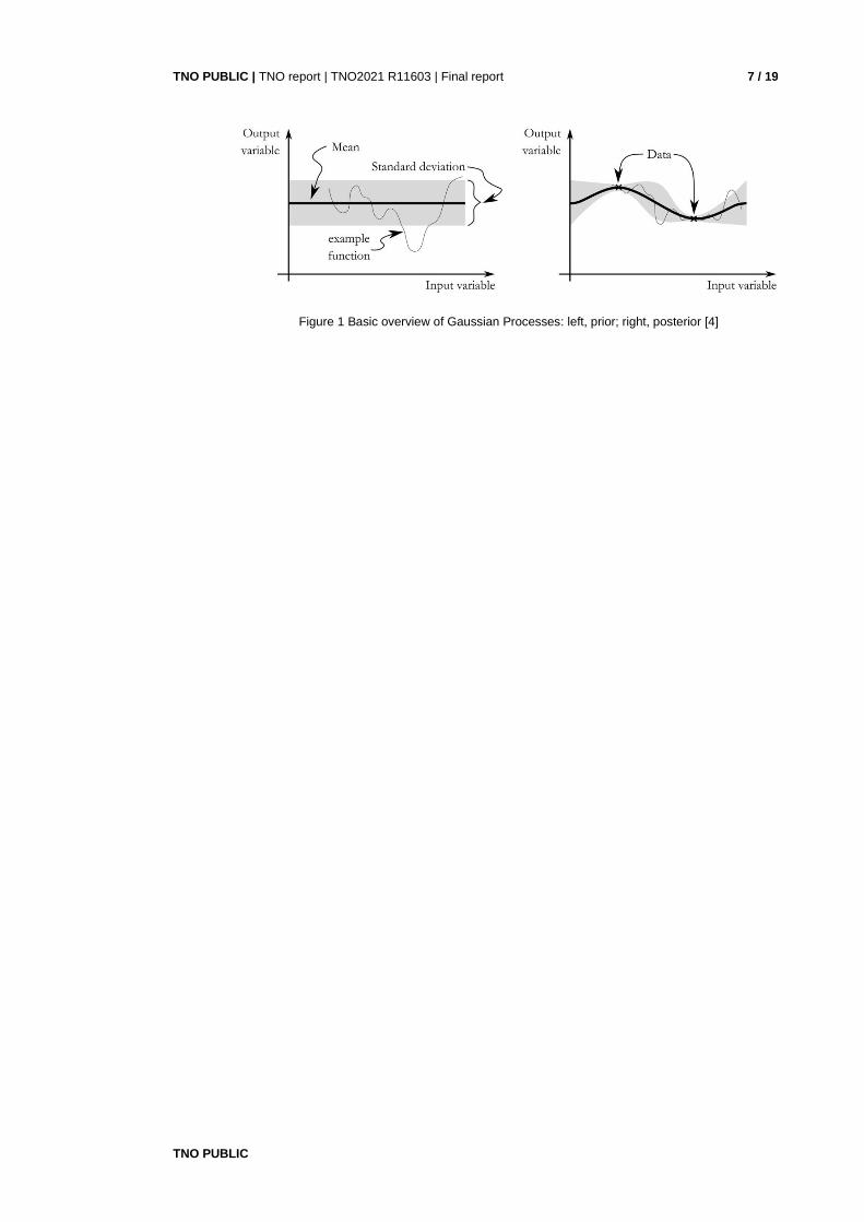
As described in [4], TNO wind energy has developed a novel ML algorithm based on

GP regression to remove the assumptions when producing 3D wind fields from lidar

measurements. This algorithm is naturally robust to overfitting and predicts

uncertainty in the prediction derived from data density and machine error. In a GP, it

is assumed that variables in a stochastic process are jointly normally distributed, and

can be described as such. A GP is fully specified by a mean and a covariance

function, and can be fitted to any variable as illustrated in Figure 1. These properties

allow the machine learning algorithm to predict anywhere in the input space and time,

essentially turning it into a powerful regression tool. As such, GP provides a number

of powerful benefits:

• prediction of higher-frequency data,

• interpolation of missing data,

• spatial prediction of data within the measurement volume and

• calculation of prediction uncertainty is included in the process itself.

The main limitation of GP are its bias towards the mean when predicting away from

measurement data.

An additional limitation to the overall methodology is in regards to how the GP is used.

They predict radial wind speeds, and so conversion to horizontal wind speed (HWS)

is highly dependent on the methodology used.

TNO PUBLIC


Figure 1 Basic overview of Gaussian Processes: left, prior; right, posterior [4]

TNO PUBLIC


3 Turbulence Intensity calculation

TNO has been working with different types of lidar, including GBL and scanning lidar

configurations. While HWS is resolved well by lidar systems, TI continues to be a

challenge topic. Specifically, the TI measured by lidar is not as the same as that

measured by a cup or sonic anemometer due to volume-averaging (as mentioned in

2.2). In this report, a two-beam NML is considered to apply the GP. The purpose of

the works is to assess the ability for a GP to improve TI measurement from a NML.

The following goals are considered:

• apply the GP to a two-beam NML, producing wind statistics,

• analyse the effect of the GP on lidar-based TI predictions, and

• explore potential ways to improve the TI calculations, using the GP.

3.1 Wind dataset

The dataset used for this campaign is that for the Lawine campaign [5]. The details

of this campaign, including information on the installation, can be found in the

instrumentation report [6]. A two-beam Wind Iris lidar was installed on a turbine in

order to investigate turbine performance. The flat terrain and proximity to a MM

makes this an ideal dataset to test the GP on.

An 8-hour analysis period was chosen when the wind was aligned in the direction

from the mast to the turbine, unobstructed, at high wind speeds (above 10 m/s).

During this period, the lidar was also configured to measure at a distance equal to

that between the turbine and the mast. If the turbine was pointing 15° offset from the

mast direction, one of the two lidar beams would be measuring at the MM location.

As such, filters on the data were:

• Measurement sector: During the 8-hour period, the wind was consistent, flowing

from the south-west, ensuring it passed the MM prior to reaching the wind turbine.

As such, with the lidar mounted on the turbine, it would always point close to the

MM within the period.

• Wind speed: The period analyzed had wind speeds above the rated wind speed

of the mounted turbine, ensuring the lidar would be facing the correct direction.

Specifically, ten-minute averaged HWS from the MM was never recorded as

lower than 10 m/s.

• lidar status: The lidar itself must be outputting an operational status for all ranges

so the signals in Table 1 should be available.

• CNR Value: The CNR was bounded by -22 dB on the lower end and -3 dB on the

upper end. High values of the CNR values indicate obstruction of the lidar beam

(such as by the MM itself), while low values indicate atmospheric events, which

can affect results.

Table 1 below shows the measured signals from the WindIris lidar, while Table 2

shows the same used from the met mast. Table 3 provides a list and description of

all outputs from the WindIris lidar.

TNO PUBLIC


Table 1 Measured signals WindIris

Measured signals WindIris

Description Short name Sampling rate [Hz.] Unit

Tilt T6_WI_tilt 1 °

Roll T6_WI_roll 1 °

Description For every height

Short name xx = 1 (80m), 2 (120m), 3 (160m), 4 (200m), 5 (240m), 6 (280m), 7 (320m), 8 (360m), 9 (400m), 10 (440m)

Sampling rate [Hz.] Unit

Line of sight T6_WI_Dxx_los 1 [-]

Horizontal wind speed T6_WI_Dxx_ws 1 m/s

Wind direction T6_WI_Dxx_wd 1 °

Radial wind speed T6_WI_Dxx_rws 1 m/s

Radial wind speed deviation T6_WI_Dxx_rws_dev 1 m/s

Carrier to noise ratio T6_WI_Dxx_cnr 1 dB

Radial wind speed status T6_WI_Dxx_rws_st 1 [-]

Overrun Status T6_WI_Dxx_overrun_st 1 [-]

Horizontal wind speed status T6_WI_Dxx_ws_st 1 [-]

Time T6_WI_Dxx_TIME 1 ms

Table 2 Hub height measured signals - MM

Hub height measured signals meteorological mast

Description Short name Sampling rate

[Hz.] Unit

Wind speed, 120deg boom MM3_WS80_120 4 m/s

Wind speed, 240deg boom MM3_WS80_240 4 m/s

Sonic wind speed, u component MM3_S80N_U

4

m/s

Sonic wind speed, v component MM3_S80N_V m/s

Sonic wind speed, w component MM3_S80N_W m/s

Sonic wind speed, status MM3_S80N_St [-]

Air temp MM3_Tair80 4 °C

Humidity MM3_RH80 4 %

Air pressure MM3_Pair80 4 hPa

Wind direction, 120deg boom MM3_WD80_120 4 °

Wind direction, 240deg boom MM3_WD80_240 4 °

TNO PUBLIC


Table 3 WindIris lidar output description

3.2 Wind field reconstruction

As the limitation of a single lidar to distinguish horizontal wind shear and wind

direction at the same time (cyclops dilemma), the wind flow is assumed as

homogeneous on horizontal plane without wind shear. The WindIris lidar measures

consecutively radial wind speeds on its two lines of sight (LOS) and reconstructs

HWS and direction based on these two consecutive radial wind speed

measurements. Remembering that the wind has three components with respect to

three directions, there are now two equations and three unknowns. In order to solve

the equations, the vertical wind component of wind is assumed null.

The wind filed reconstruction is illustrated as in Figure 2. 𝑣𝐿𝑂𝑆 is the measured LOS

radial wind speed. 𝑢, 𝑣 are the wind speed component on horizontal X and Y direction

respectively. 𝑢ℎ is the calculated HWS and 𝛾 is the calculated wind direction. This

reconstruction is performed on the 10-minute average values of the radial wind

speeds, as reconstructing on instantaneous values tends to skew HWS results, as

shown later in the report. Finally, individual beam TI is calculated as the standard

deviation of the radial wind speed divided by the average over ten minutes. For the

wind field, the TI is the average between the individual beam TI’s.

Figure 2: Wind field reconstruction [7]

TNO PUBLIC


Considering the measured LOS radial speeds in space and time are variables, a GP

is fitted to them. Then velocities at any space and time can be predicted [4] and a 2D

(based on a 2-beams lidar) wind field can be reconstructed.

3.3 GP implementation

Data between the turbine, met mast, and lidar were combined and synchronized, to

provide a robust analysis, and the GP’s were successfully applied to this dataset.

The GP implementation pipeline:

1. For every 60 seconds of data, fit a GP’s hyper-parameters to the provided

times, locations, and radial wind speed data. These are considered training

GP1’s

2. Use a second GP layer to smoothen the hyper-parameters from the training

GP1’s. These are considered the GP2.

3. Using the GP2, predict hyper-parameters for individual 30-second,

overlapping GP1’s at the requested times/locations. These are considered

prediction GP1’s

4. Finally, using these parameters, generate radial wind speed predictions from

each prediction GP1, obtaining the requested radial wind field

Figure 3: GP implementation pipeline

3.4 Results

3.4.1 Initialization of the GP’s

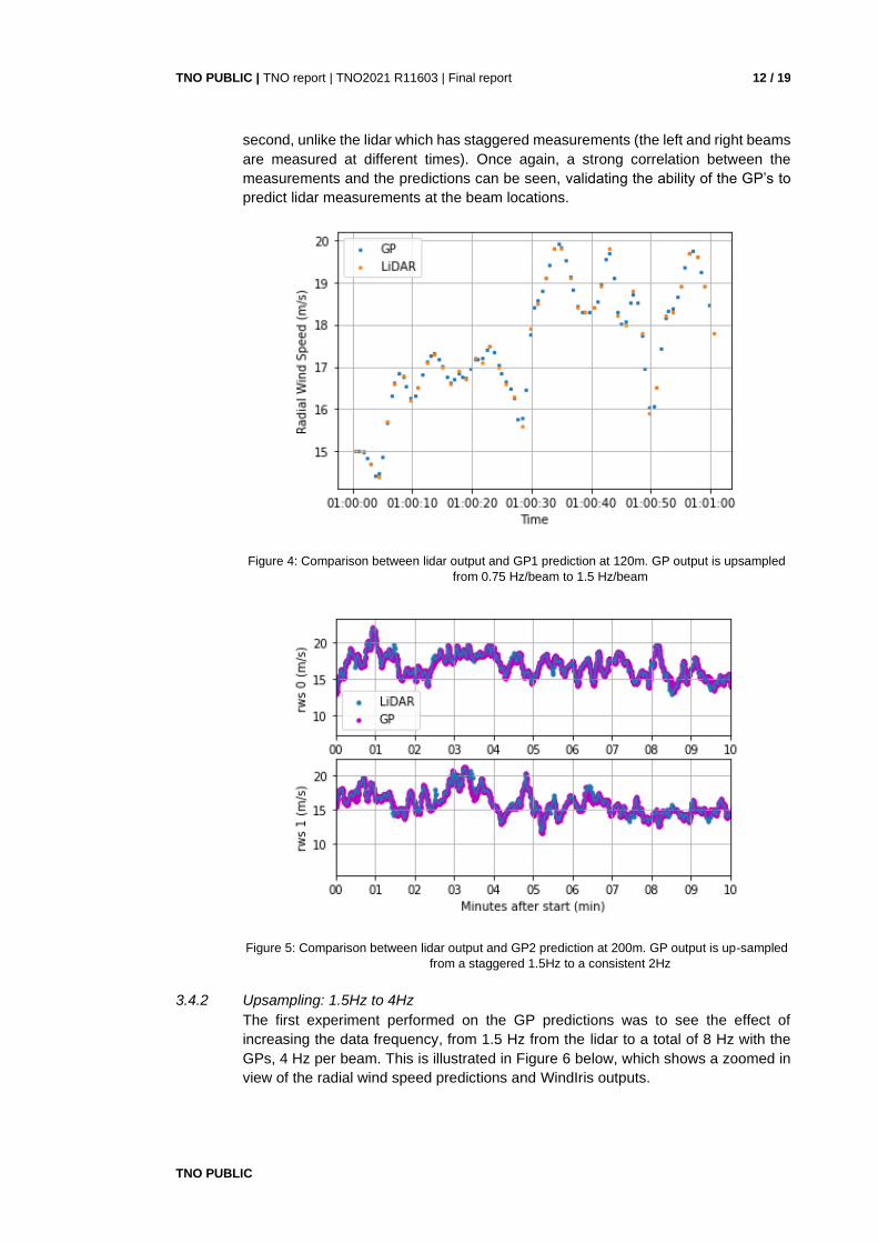
Figure 4 and Figure 5 below show the outputs of the GP process. The first figure

shows 60 seconds of LOS radial wind speeds utilizing a training GP1 to predict at

one lidar beam location. This is prior to having smoothened hyper-parameters from

a GP2. It can be seen that the GP is able to up-sample the lidar measurements of a

single beam accurately, following the overall trends of the measurement equipment.

Figure 5 on the other hand shows the output at two beam locations for the overall

process: utilizing training GP1’s, overarching GP2’s, and prediction GP1’s. Here, up-

sampling was done in order to provide a lidar prediction for each beam at every

TNO PUBLIC


second, unlike the lidar which has staggered measurements (the left and right beams

are measured at different times). Once again, a strong correlation between the

measurements and the predictions can be seen, validating the ability of the GP’s to

predict lidar measurements at the beam locations.

Figure 4: Comparison between lidar output and GP1 prediction at 120m. GP output is upsampled

from 0.75 Hz/beam to 1.5 Hz/beam

Figure 5: Comparison between lidar output and GP2 prediction at 200m. GP output is up-sampled

from a staggered 1.5Hz to a consistent 2Hz

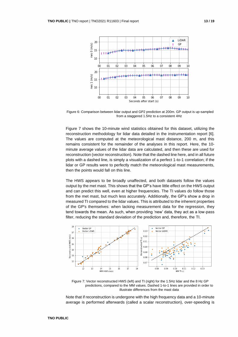
3.4.2 Upsampling: 1.5Hz to 4Hz

The first experiment performed on the GP predictions was to see the effect of

increasing the data frequency, from 1.5 Hz from the lidar to a total of 8 Hz with the

GPs, 4 Hz per beam. This is illustrated in Figure 6 below, which shows a zoomed in

view of the radial wind speed predictions and WindIris outputs.

TNO PUBLIC


Figure 6: Comparison between lidar output and GP2 prediction at 200m. GP output is up-sampled

from a staggered 1.5Hz to a consistent 4Hz

Figure 7 shows the 10-minute wind statistics obtained for this dataset, utilizing the

reconstruction methodology for lidar data detailed in the instrumentation report [6].

The values are computed at the meteorological mast distance, 200 m, and this

remains consistent for the remainder of the analyses in this report. Here, the 10-

minute average values of the lidar data are calculated, and then these are used for

reconstruction (vector reconstruction). Note that the dashed line here, and in all future

plots with a dashed line, is simply a visualization of a perfect 1-to-1 correlation; if the

lidar or GP results were to perfectly match the meteorological mast measurements,

then the points would fall on this line.

The HWS appears to be broadly unaffected, and both datasets follow the values

output by the met mast. This shows that the GP’s have little effect on the HWS output

and can predict this well, even at higher frequencies. The TI values do follow those

from the met mast, but much less accurately. Additionally, the GP’s show a drop in

measured TI compared to the lidar values. This is attributed to the inherent properties

of the GP's themselves: when lacking measurement data for the regression, they

tend towards the mean. As such, when providing ‘new’ data, they act as a low-pass

filter, reducing the standard deviation of the prediction and, therefore, the TI.

Figure 7: Vector reconstructed HWS (left) and TI (right) for the 1.5Hz lidar and the 8 Hz GP

predictions, compared to the MM values. Dashed 1-to-1 lines are provided in order to

illustrate differences from the mast data

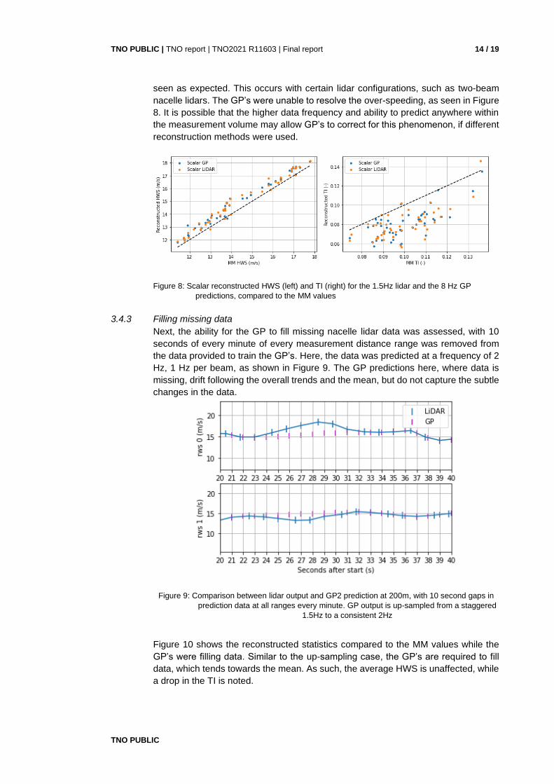
Note that if reconstruction is undergone with the high frequency data and a 10-minute

average is performed afterwards (called a scalar reconstruction), over-speeding is

TNO PUBLIC


seen as expected. This occurs with certain lidar configurations, such as two-beam

nacelle lidars. The GP’s were unable to resolve the over-speeding, as seen in Figure

8. It is possible that the higher data frequency and ability to predict anywhere within

the measurement volume may allow GP’s to correct for this phenomenon, if different

reconstruction methods were used.

Figure 8: Scalar reconstructed HWS (left) and TI (right) for the 1.5Hz lidar and the 8 Hz GP

predictions, compared to the MM values

3.4.3 Filling missing data

Next, the ability for the GP to fill missing nacelle lidar data was assessed, with 10

seconds of every minute of every measurement distance range was removed from

the data provided to train the GP’s. Here, the data was predicted at a frequency of 2

Hz, 1 Hz per beam, as shown in Figure 9. The GP predictions here, where data is

missing, drift following the overall trends and the mean, but do not capture the subtle

changes in the data.

Figure 9: Comparison between lidar output and GP2 prediction at 200m, with 10 second gaps in

prediction data at all ranges every minute. GP output is up-sampled from a staggered

1.5Hz to a consistent 2Hz

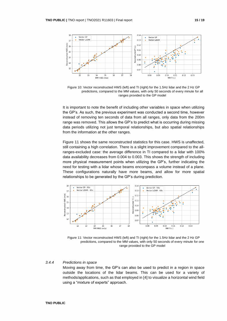
Figure 10 shows the reconstructed statistics compared to the MM values while the

GP’s were filling data. Similar to the up-sampling case, the GP’s are required to fill

data, which tends towards the mean. As such, the average HWS is unaffected, while

a drop in the TI is noted.

TNO PUBLIC



predictions, compared to the MM values, with only 50 seconds of every minute for all

ranges provided to the GP model

It is important to note the benefit of including other variables in space when utilizing

the GP’s. As such, the previous experiment was conducted a second time, however

instead of removing ten seconds of data from all ranges, only data from the 200m

range was removed. This allows the GP’s to predict what is occurring during missing

data periods utilizing not just temporal relationships, but also spatial relationships

from the information at the other ranges.

Figure 11 shows the same reconstructed statistics for this case. HWS is unaffected,

still containing a high correlation. There is a slight improvement compared to the all-

ranges-excluded case: the average difference in TI compared to a lidar with 100%

data availability decreases from 0.004 to 0.003. This shows the strength of including

more physical measurement points when utilizing the GP’s, further indicating the

need for testing with a lidar whose beams encompass a volume instead of a plane.

These configurations naturally have more beams, and allow for more spatial

relationships to be generated by the GP’s during prediction.


predictions, compared to the MM values, with only 50 seconds of every minute for one

range provided to the GP model

3.4.4 Predictions in space

Moving away from time, the GP’s can also be used to predict in a region in space

outside the locations of the lidar beams. This can be used for a variety of

methods/applications, such as that employed in [4] to visualize a horizontal wind field

using a “mixture of experts” approach.

TNO PUBLIC


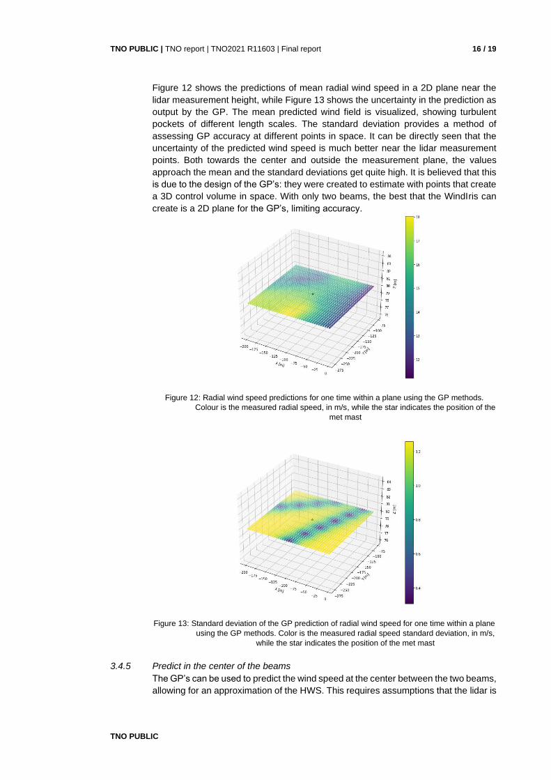
Figure 12 shows the predictions of mean radial wind speed in a 2D plane near the

lidar measurement height, while Figure 13 shows the uncertainty in the prediction as

output by the GP. The mean predicted wind field is visualized, showing turbulent

pockets of different length scales. The standard deviation provides a method of

assessing GP accuracy at different points in space. It can be directly seen that the

uncertainty of the predicted wind speed is much better near the lidar measurement

points. Both towards the center and outside the measurement plane, the values

approach the mean and the standard deviations get quite high. It is believed that this

is due to the design of the GP’s: they were created to estimate with points that create

a 3D control volume in space. With only two beams, the best that the WindIris can

create is a 2D plane for the GP’s, limiting accuracy.

Figure 12: Radial wind speed predictions for one time within a plane using the GP methods.

Colour is the measured radial speed, in m/s, while the star indicates the position of the

met mast

Figure 13: Standard deviation of the GP prediction of radial wind speed for one time within a plane

using the GP methods. Color is the measured radial speed standard deviation, in m/s,

while the star indicates the position of the met mast

3.4.5 Predict in the center of the beams

The GP’s can be used to predict the wind speed at the center between the two beams,

allowing for an approximation of the HWS. This requires assumptions that the lidar is

TNO PUBLIC


not tilting, and that the turbine is facing directly into the wind. However, for the

purposes of this report, these can be assumed to be true in order to see how a

prediction in space with the WindIris data and how the GP’s performs.

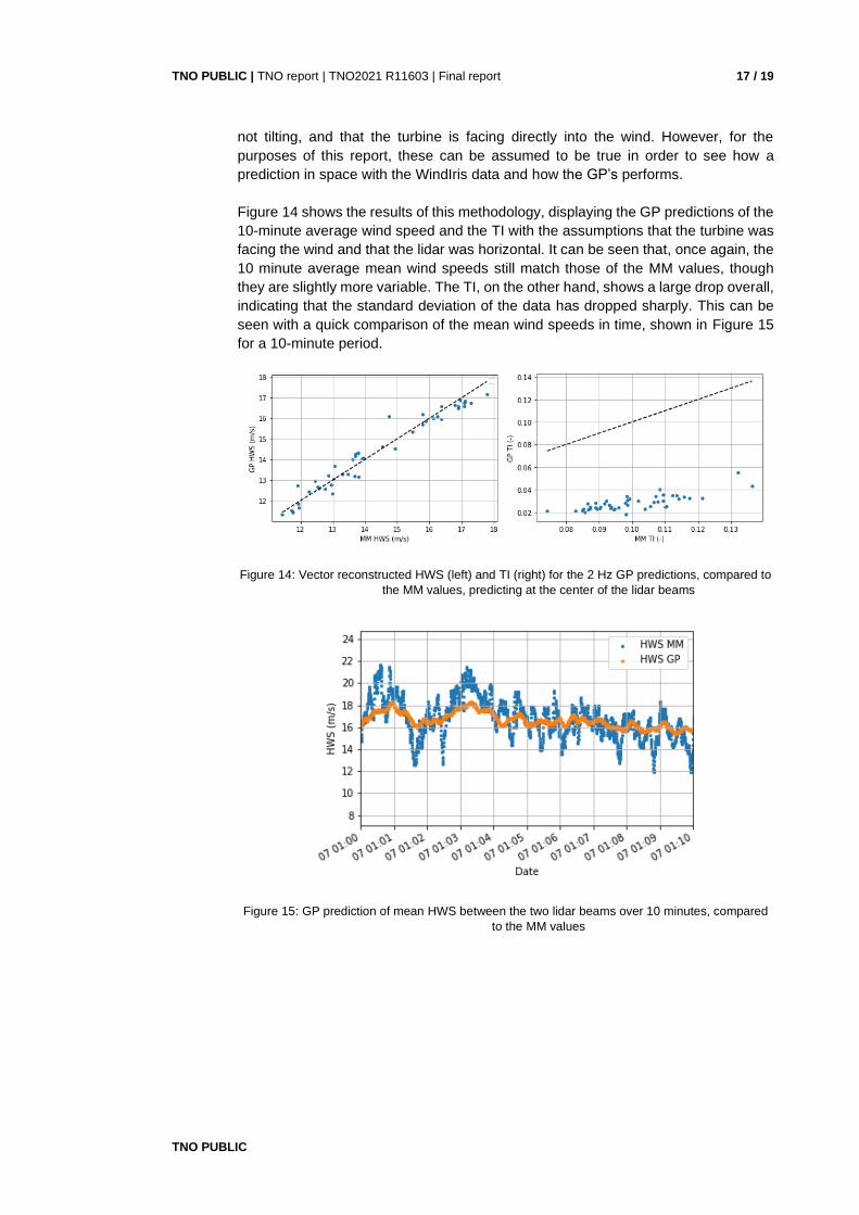
Figure 14 shows the results of this methodology, displaying the GP predictions of the

10-minute average wind speed and the TI with the assumptions that the turbine was

facing the wind and that the lidar was horizontal. It can be seen that, once again, the

10 minute average mean wind speeds still match those of the MM values, though

they are slightly more variable. The TI, on the other hand, shows a large drop overall,

indicating that the standard deviation of the data has dropped sharply. This can be

seen with a quick comparison of the mean wind speeds in time, shown in Figure 15

for a 10-minute period.

Figure 14: Vector reconstructed HWS (left) and TI (right) for the 2 Hz GP predictions, compared to

the MM values, predicting at the center of the lidar beams

Figure 15: GP prediction of mean HWS between the two lidar beams over 10 minutes, compared

to the MM values

TNO PUBLIC


4 Conclusions

The goal of this project is to explore the potentials of using GP to improve the TI

calculation for lidar wind measurements. Several different GP implementations have

been tested: up-sampling the data to higher frequency, filling missing data, predicting

in space and predicting in the center of the beams. Although GP does not show

effective improvements for calculating TI with the data from a two-beam lidar, it does

demonstrate that GP can be applied to almost any lidar system to predict LOS radial

wind speeds in space and time.

We identified the following recommendations for further exploring the application of

GP to improve lidar TI calculation:

• using lidar with more beams for predictions within a volume as opposed to a

plane,

• further research into different methods of modelling/calculating TI, and

• deeper investigation into the GP mechanics: change in GP time lengths or

overlapping GP1’s.

TNO PUBLIC


5 References

[1]. A. Sathe and J. Mann, ‘A review of turbulence measurements using ground-

based wind lidars’, Atmos. Meas. Tech., 6, 3147–3167, 2013

[2]. IEC 61400-12-1:2017, ‘Wind power generation systems - Part 12-1: Power

performance measurements of electricity producing wind turbines’.

[3]. K.Boorsma, et al, ECN-E-16-044, ‘lidar application for wind energy

efficiency’, 2016

[4]. C. Stock-Williams et al, ‘Wind filed reconstruction from lidar measurements

at high-frequency using machine learning’, J. Phys.: Conf. Ser. 1102 012003,

2018

[5]. J.W. Wagenaar, et al, ‘Turbine performance validation; the application of

nacelle LiDAR’, EWEA 2014

[6]. G. Bergman, J.W. Wagenaar and K. Boorsma, ECN-X-14-085, ‘LAWINE

instrumentation report’, Rev. 2, 2016

[7]. E. Simley, A. Scholbrock, ‘Nacelle Mounted lidar for Wind Energy

Applicaitons’, Wind Workforce Development Webinar Series, NREL, 2020

Turbulence intensity calculation using Gaussian Processes on ...

Documents