Tuning and test of fragmentation models based on identified particles and precision event shape data

EUROPEAN ORGANIZATION FOR NUCLEAR RESEARCH

CERN{PPE/96-120

22 August 1996

Tuning and Test of Fragmentation

Models Based on Identi�ed Particles

and Precision Event Shape Data

DELPHI Collaboration

Abstract

Event shape and charged particle inclusive distributions are measured using750000 decays of the Z to hadrons from the DELPHI detector at LEP. Theseprecise data allow a decisive confrontation with models of the hadronizationprocess. Improved tunings of the JETSET, ARIADNE and HERWIG partonshower models and the JETSET matrix element model are obtained by �ttingthe models to these DELPHI data as well as to identi�ed particle distributionsfrom all LEP experiments. The description of the data distributions by themodels is critically reviewed with special importance attributed to identi�edparticles.

(To be submitted to Zeit. Phys. C)

ii

P.Abreu21, W.Adam50, T.Adye37, I.Ajinenko42 , G.D.Alekseev16, R.Alemany49, P.P.Allport22 , S.Almehed24 ,U.Amaldi9, S.Amato47, A.Andreazza28, M.L.Andrieux14, P.Antilogus9 , W-D.Apel17, B.�Asman44,J-E.Augustin25 , A.Augustinus9 , P.Baillon9 , P.Bambade19, F.Barao21, R.Barate14, M.Barbi47, D.Y.Bardin16 ,A.Baroncelli40 , O.Barring24, J.A.Barrio26, W.Bartl50 , M.J.Bates37, M.Battaglia15 , M.Baubillier23 , J.Baudot39,K-H.Becks52, M.Begalli6 , P.Beilliere8 , Yu.Belokopytov9;53 , K.Belous42 , A.C.Benvenuti5 , M.Berggren47 ,D.Bertini25 , D.Bertrand2, M.Besancon39 , F.Bianchi45 , M.Bigi45 , M.S.Bilenky16 , P.Billoir23 , D.Bloch10 ,M.Blume52 , T.Bolognese39 , M.Bonesini28 , W.Bonivento28 , P.S.L.Booth22, C.Bosio40, O.Botner48,E.Boudinov31 , B.Bouquet19 , C.Bourdarios9 , T.J.V.Bowcock22, M.Bozzo13, P.Branchini40 , K.D.Brand36,T.Brenke52, R.A.Brenner15, C.Bricman2 , R.C.A.Brown9, P.Bruckman18, J-M.Brunet8, L.Bugge33, T.Buran33,T.Burgsmueller52 , P.Buschmann52 , A.Buys9, S.Cabrera49 , M.Caccia28, M.Calvi28 , A.J.Camacho Rozas41 ,T.Camporesi9, V.Canale38, M.Canepa13 , K.Cankocak44, F.Cao2, F.Carena9, L.Carroll22, C.Caso13,M.V.Castillo Gimenez49 , A.Cattai9, F.R.Cavallo5 , V.Chabaud9, Ph.Charpentier9 , L.Chaussard25, P.Checchia36 ,G.A.Chelkov16, M.Chen2, R.Chierici45 , P.Chliapnikov42 , P.Chochula7 , V.Chorowicz9, J.Chudoba30, V.Cindro43 ,P.Collins9 , J.L.Contreras19, R.Contri13 , E.Cortina49, G.Cosme19, F.Cossutti46, J-H.Cowell22, H.B.Crawley1,D.Crennell37 , G.Crosetti13, J.Cuevas Maestro34 , S.Czellar15 , E.Dahl-Jensen29 , J.Dahm52, B.Dalmagne19 ,M.Dam29, G.Damgaard29 , P.D.Dauncey37 , M.Davenport9, W.Da Silva23 , C.Defoix8, A.Deghorain2 ,G.Della Ricca46, P.Delpierre27 , N.Demaria35 , A.De Angelis9 , W.De Boer17, S.De Brabandere2 , C.De Clercq2,C.De La Vaissiere23 , B.De Lotto46, A.De Min36, L.De Paula47 , C.De Saint-Jean39 , H.Dijkstra9, L.Di Ciaccio38 ,A.Di Diodato38 , F.Djama10, J.Dolbeau8 , M.Donszelmann9 , K.Doroba51 , M.Dracos10, J.Drees52, K.-A.Drees52,M.Dris32 , J-D.Durand25 , D.Edsall1 , R.Ehret17, G.Eigen4 , T.Ekelof48, G.Ekspong44 , M.Elsing52 , J-P.Engel10,B.Erzen43, M.Espirito Santo21, E.Falk24, D.Fassouliotis32 , M.Feindt9 , A.Ferrer49, S.Fichet23 , T.A.Filippas32 ,A.Firestone1, P.-A.Fischer10, H.Foeth9, E.Fokitis32 , F.Fontanelli13 , F.Formenti9, B.Franek37, P.Frenkiel8 ,D.C.Fries17, A.G.Frodesen4, R.Fruhwirth50 , F.Fulda-Quenzer19 , J.Fuster49, A.Galloni22 , D.Gamba45 ,M.Gandelman6 , C.Garcia49, J.Garcia41, C.Gaspar9, U.Gasparini36 , Ph.Gavillet9 , E.N.Gazis32, D.Gele10 ,J-P.Gerber10, R.Gokieli51 , B.Golob43 , G.Gopal37, L.Gorn1, M.Gorski51 , Yu.Gouz45;53 , V.Gracco13,E.Graziani40 , C.Green22, A.Grefrath52, P.Gris39, G.Grosdidier19 , K.Grzelak51, S.Gumenyuk28;53 ,P.Gunnarsson44 , M.Gunther48, J.Guy37, F.Hahn9, S.Hahn52, Z.Hajduk18 , A.Hallgren48 , K.Hamacher52,F.J.Harris35, V.Hedberg24, R.Henriques21 , J.J.Hernandez49, P.Herquet2, H.Herr9, T.L.Hessing35, E.Higon49 ,H.J.Hilke9, T.S.Hill1 , S-O.Holmgren44 , P.J.Holt35, D.Holthuizen31 , S.Hoorelbeke2 , M.Houlden22 , J.Hrubec50,K.Huet2, K.Hultqvist44 , J.N.Jackson22, R.Jacobsson44 , P.Jalocha18 , R.Janik7 , Ch.Jarlskog24 , G.Jarlskog24 ,P.Jarry39, B.Jean-Marie19, E.K.Johansson44 , L.Jonsson24, P.Jonsson24 , C.Joram9, P.Juillot10 , M.Kaiser17 ,F.Kapusta23, K.Karafasoulis11 , M.Karlsson44 , E.Karvelas11 , S.Katsanevas3 , E.C.Katsou�s32, R.Keranen4,Yu.Khokhlov42 , B.A.Khomenko16, N.N.Khovanski16, B.King22 , N.J.Kjaer31, O.Klapp52, H.Klein9 , A.Klovning4 ,P.Kluit31 , B.Koene31, P.Kokkinias11 , M.Koratzinos9 , K.Korcyl18, V.Kostioukhine42 , C.Kourkoumelis3 ,O.Kouznetsov13;16 , C.Kreuter17, I.Kronkvist24 , Z.Krumstein16 , W.Krupinski18 , P.Kubinec7, W.Kucewicz18 ,K.Kurvinen15 , C.Lacasta49, I.Laktineh25 , J.W.Lamsa1, L.Lanceri46, D.W.Lane1, P.Langefeld52, V.Lapin42 ,J-P.Laugier39, R.Lauhakangas15 , G.Leder50, F.Ledroit14, V.Lefebure2, C.K.Legan1, R.Leitner30, J.Lemonne2,G.Lenzen52, V.Lepeltier19 , T.Lesiak18, J.Libby35, D.Liko50, R.Lindner52 , A.Lipniacka44 , I.Lippi36 ,B.Loerstad24, J.G.Loken35, J.M.Lopez41, D.Loukas11 , P.Lutz39, L.Lyons35, J.MacNaughton50, G.Maehlum17 ,J.R.Mahon6, A.Maio21, T.G.M.Malmgren44, V.Malychev16 , F.Mandl50 , J.Marco41, R.Marco41, B.Marechal47 ,M.Margoni36 , J-C.Marin9, C.Mariotti40 , A.Markou11, C.Martinez-Rivero41 , F.Martinez-Vidal49 ,S.Marti i Garcia22 , J.Masik30, F.Matorras41, C.Matteuzzi28 , G.Matthiae38 , M.Mazzucato36 , M.Mc Cubbin9 ,R.Mc Kay1, R.Mc Nulty22, J.Medbo48, M.Merk31, C.Meroni28 , S.Meyer17, W.T.Meyer1, A.Miagkov42 ,M.Michelotto36 , E.Migliore45 , L.Mirabito25 , W.A.Mitaro�50 , U.Mjoernmark24, T.Moa44, R.Moeller29 ,K.Moenig52 , M.R.Monge13 , P.Morettini13 , H.Mueller17 , M.Mulders31 , L.M.Mundim6 , W.J.Murray37,B.Muryn18 , G.Myatt35, F.Naraghi14, F.L.Navarria5, S.Navas49, K.Nawrocki51, P.Negri28, W.Neumann52 ,N.Neumeister50, R.Nicolaidou3 , B.S.Nielsen29 , M.Nieuwenhuizen31 , V.Nikolaenko10 , P.Niss44, A.Nomerotski36 ,A.Normand35, W.Oberschulte-Beckmann17 , V.Obraztsov42, A.G.Olshevski16 , A.Onofre21, R.Orava15,K.Osterberg15, A.Ouraou39, P.Paganini19 , M.Paganoni9;28 , P.Pages10, R.Pain23 , H.Palka18 ,Th.D.Papadopoulou32 , K.Papageorgiou11 , L.Pape9, C.Parkes35, F.Parodi13 , A.Passeri40 , M.Pegoraro36 ,L.Peralta21, H.Pernegger50, M.Pernicka50 , A.Perrotta5, C.Petridou46 , A.Petrolini13 , M.Petrovyck42 ,H.T.Phillips37 , G.Piana13 , F.Pierre39, S.Plaszczynski19 , O.Podobrin17 , M.E.Pol6, G.Polok18 , P.Poropat46,V.Pozdniakov16 , P.Privitera38 , N.Pukhaeva16 , A.Pullia28 , D.Radojicic35 , S.Ragazzi28 , H.Rahmani32 , J.Rames12,P.N.Rato�20, A.L.Read33, M.Reale52 , P.Rebecchi19 , N.G.Redaelli28 , M.Regler50 , D.Reid9, P.B.Renton35,L.K.Resvanis3, F.Richard19 , J.Richardson22 , J.Ridky12 , G.Rinaudo45 , I.Ripp39 , A.Romero45, I.Roncagliolo13 ,P.Ronchese36 , L.Roos14, E.I.Rosenberg1 , E.Rosso9, P.Roudeau19, T.Rovelli5 , W.Ruckstuhl31 ,V.Ruhlmann-Kleider39 , A.Ruiz41, K.Rybicki18 , H.Saarikko15 , Y.Sacquin39 , A.Sadovsky16 , O.Sahr14, G.Sajot14,J.Salt49, J.Sanchez26 , M.Sannino13 , M.Schimmelpfennig17 , H.Schneider17 , U.Schwickerath17, M.A.E.Schyns52,G.Sciolla45 , F.Scuri46, P.Seager20, Y.Sedykh16, A.M.Segar35, A.Seitz17 , R.Sekulin37 , L.Serbelloni38 ,R.C.Shellard6 , P.Siegrist39 , R.Silvestre39 , S.Simonetti39 , F.Simonetto36, A.N.Sisakian16 , B.Sitar7, T.B.Skaali33 ,G.Smadja25, N.Smirnov42 , O.Smirnova24 , G.R.Smith37 , A.Sokolov42 , R.Sosnowski51 , D.Souza-Santos6 ,T.Spassov21, E.Spiriti40 , P.Sponholz52 , S.Squarcia13 , C.Stanescu40, S.Stapnes33, I.Stavitski36 , K.Stevenson35 ,F.Stichelbaut9 , A.Stocchi19, J.Strauss50, R.Strub10, B.Stugu4, M.Szczekowski51 , M.Szeptycka51, T.Tabarelli28 ,

iii

J.P.Tavernet23, O.Tchikilev42 , J.Thomas35, A.Tilquin27 , J.Timmermans31, L.G.Tkatchev16, T.Todorov10,S.Todorova10, D.Z.Toet31, A.Tomaradze2, B.Tome21, A.Tonazzo28, L.Tortora40, G.Transtromer24, D.Treille9 ,W.Trischuk9 , G.Tristram8, A.Trombini19, C.Troncon28, A.Tsirou9, M-L.Turluer39, I.A.Tyapkin16, M.Tyndel37 ,S.Tzamarias22 , B.Ueberschaer52, O.Ullaland9 , V.Uvarov42, G.Valenti5, E.Vallazza9 , G.W.Van Apeldoorn31 ,P.Van Dam31, J.Van Eldik31 , N.Vassilopoulos35 , G.Vegni28 , L.Ventura36, W.Venus37, F.Verbeure2, M.Verlato36,L.S.Vertogradov16, D.Vilanova39 , P.Vincent25, L.Vitale46 , E.Vlasov42 , A.S.Vodopyanov16 , V.Vrba12,H.Wahlen52 , C.Walck44, F.Waldner46 , M.Weierstall52 , P.Weilhammer9 , C.Weiser17 , A.M.Wetherell9 , D.Wicke52 ,J.H.Wickens2, M.Wielers17 , G.R.Wilkinson35 , W.S.C.Williams35 , M.Winter10 , M.Witek18 , K.Woschnagg48 ,K.Yip35, O.Yushchenko42 , F.Zach25, A.Zaitsev42 , A.Zalewska9, P.Zalewski51 , D.Zavrtanik43 , E.Zevgolatakos11 ,N.I.Zimin16 , M.Zito39 , D.Zontar43, G.C.Zucchelli44 , G.Zumerle36

1Department of Physics and Astronomy, Iowa State University, Ames IA 50011-3160, USA

2Physics Department, Univ. Instelling Antwerpen, Universiteitsplein 1, B-2610 Wilrijk, Belgium

and IIHE, ULB-VUB, Pleinlaan 2, B-1050 Brussels, Belgium

and Facult�e des Sciences, Univ. de l'Etat Mons, Av. Maistriau 19, B-7000 Mons, Belgium3Physics Laboratory, University of Athens, Solonos Str. 104, GR-10680 Athens, Greece

4Department of Physics, University of Bergen, All�egaten 55, N-5007 Bergen, Norway

5Dipartimento di Fisica, Universit�a di Bologna and INFN, Via Irnerio 46, I-40126 Bologna, Italy

6Centro Brasileiro de Pesquisas F�isicas, rua Xavier Sigaud 150, RJ-22290 Rio de Janeiro, Brazil

and Depto. de F�isica, Pont. Univ. Cat�olica, C.P. 38071 RJ-22453 Rio de Janeiro, Brazil

and Inst. de F�isica, Univ. Estadual do Rio de Janeiro, rua S~ao Francisco Xavier 524, Rio de Janeiro, Brazil

7Comenius University, Faculty of Mathematics and Physics, Mlynska Dolina, SK-84215 Bratislava, Slovakia

8Coll�ege de France, Lab. de Physique Corpusculaire, IN2P3-CNRS, F-75231 Paris Cedex 05, France9CERN, CH-1211 Geneva 23, Switzerland

10Centre de Recherche Nucl�eaire, IN2P3 - CNRS/ULP - BP20, F-67037 Strasbourg Cedex, France

11Institute of Nuclear Physics, N.C.S.R. Demokritos, P.O. Box 60228, GR-15310 Athens, Greece

12FZU, Inst. of Physics of the C.A.S. High Energy Physics Division, Na Slovance 2, 180 40, Praha 8, Czech Republic

13Dipartimento di Fisica, Universit�a di Genova and INFN, Via Dodecaneso 33, I-16146 Genova, Italy14Institut des Sciences Nucl�eaires, IN2P3-CNRS, Universit�e de Grenoble 1, F-38026 Grenoble Cedex, France

15Research Institute for High Energy Physics, SEFT, P.O. Box 9, FIN-00014 Helsinki, Finland

16Joint Institute for Nuclear Research, Dubna, Head Post O�ce, P.O. Box 79, 101 000 Moscow, Russian Federation

17Institut f�ur Experimentelle Kernphysik, Universit�at Karlsruhe, Postfach 6980, D-76128 Karlsruhe, Germany

18Institute of Nuclear Physics and University of Mining and Metalurgy, Ul. Kawiory 26a, PL-30055 Krakow, Poland

19Universit�e de Paris-Sud, Lab. de l'Acc�el�erateur Lin�eaire, IN2P3-CNRS, Bat. 200, F-91405 Orsay Cedex, France

20School of Physics and Chemistry, University of Lancaster, Lancaster LA1 4YB, UK21LIP, IST, FCUL - Av. Elias Garcia, 14-1

o, P-1000 Lisboa Codex, Portugal

22Department of Physics, University of Liverpool, P.O. Box 147, Liverpool L69 3BX, UK

23LPNHE, IN2P3-CNRS, Universit�es Paris VI et VII, Tour 33 (RdC), 4 place Jussieu, F-75252 Paris Cedex 05, France24Department of Physics, University of Lund, S�olvegatan 14, S-22363 Lund, Sweden

25Universit�e Claude Bernard de Lyon, IPNL, IN2P3-CNRS, F-69622 Villeurbanne Cedex, France26Universidad Complutense, Avda. Complutense s/n, E-28040 Madrid, Spain

27Univ. d'Aix - Marseille II - CPP, IN2P3-CNRS, F-13288 Marseille Cedex 09, France

28Dipartimento di Fisica, Universit�a di Milano and INFN, Via Celoria 16, I-20133 Milan, Italy

29Niels Bohr Institute, Blegdamsvej 17, DK-2100 Copenhagen 0, Denmark

30NC, Nuclear Centre of MFF, Charles University, Areal MFF, V Holesovickach 2, 180 00, Praha 8, Czech Republic

31NIKHEF, Postbus 41882, NL-1009 DB Amsterdam, The Netherlands

32National Technical University, Physics Department, Zografou Campus, GR-15773 Athens, Greece

33Physics Department, University of Oslo, Blindern, N-1000 Oslo 3, Norway34Dpto. Fisica, Univ. Oviedo, C/P. P�erez Casas, S/N-33006 Oviedo, Spain

35Department of Physics, University of Oxford, Keble Road, Oxford OX1 3RH, UK

36Dipartimento di Fisica, Universit�a di Padova and INFN, Via Marzolo 8, I-35131 Padua, Italy

37Rutherford Appleton Laboratory, Chilton, Didcot OX11 OQX, UK

38Dipartimento di Fisica, Universit�a di Roma II and INFN, Tor Vergata, I-00173 Rome, Italy39CEA, DAPNIA/Service de Physique des Particules, CE-Saclay, F-91191 Gif-sur-Yvette Cedex, France

40Istituto Superiore di Sanit�a, Ist. Naz. di Fisica Nucl. (INFN), Viale Regina Elena 299, I-00161 Rome, Italy41Instituto de Fisica de Cantabria (CSIC-UC), Avda. los Castros, S/N-39006 Santander, Spain, (CICYT-AEN93-0832)

42Inst. for High Energy Physics, Serpukov P.O. Box 35, Protvino, (Moscow Region), Russian Federation

43J. Stefan Institute and Department of Physics, University of Ljubljana, Jamova 39, SI-61000 Ljubljana, Slovenia

44Fysikum, Stockholm University, Box 6730, S-113 85 Stockholm, Sweden

45Dipartimento di Fisica Sperimentale, Universit�a di Torino and INFN, Via P. Giuria 1, I-10125 Turin, Italy

46Dipartimento di Fisica, Universit�a di Trieste and INFN, Via A. Valerio 2, I-34127 Trieste, Italy

and Istituto di Fisica, Universit�a di Udine, I-33100 Udine, Italy47Univ. Federal do Rio de Janeiro, C.P. 68528 Cidade Univ., Ilha do Fund~ao BR-21945-970 Rio de Janeiro, Brazil

48Department of Radiation Sciences, University of Uppsala, P.O. Box 535, S-751 21 Uppsala, Sweden

49IFIC, Valencia-CSIC, and D.F.A.M.N., U. de Valencia, Avda. Dr. Moliner 50, E-46100 Burjassot (Valencia), Spain

50Institut f�ur Hochenergiephysik, �Osterr. Akad. d. Wissensch., Nikolsdorfergasse 18, A-1050 Vienna, Austria

51Inst. Nuclear Studies and University of Warsaw, Ul. Hoza 69, PL-00681 Warsaw, Poland

52Fachbereich Physik, University of Wuppertal, Postfach 100 127, D-42097 Wuppertal, Germany

53On leave of absence from IHEP Serpukhov

1

1 Introduction

Precision measurements at LEP using the hadronic �nal state, such as determinationsof the strong coupling constant �s from event shapes, the forward backward asymmetriesfor quarks, the Z mass and width, or at higher energies the W� mass, require a sat-isfactory model for the properties of the corresponding �nal states. Perturbative QCDcannot provide full theoretical insight into the transition from primary quarks to observ-able hadrons, the so-called fragmentation or hadronization process, since only the part ofthis transition involving large momentum transfer, mainly the radiation of hard gluonsor the evolution of a parton shower, is calculable perturbatively. The �nal formation ofhadrons is hidden by the increase of the strong coupling constant �s at small momentumtransfer and the ensuing failure of perturbation theory.

Guidance towards a better understanding of the hadronization process must thereforecome from detailed experimental investigations of the hadronic �nal state, includingattempts to describe this process by phenomenological models inspired by QCD. LEP Iprovides a unique and unrivaled opportunity to pursue these studies. The clean well-de�ned initial state in e+e� annihilation provides an excellent testing �eld, since the eventrate at the Z is very high, the energy is large, and the capabilities of the experimentalapparatus are much improved with respect to previous experiments.

This paper attempts to determine, for the most frequently used hadronization models,parameters which give an optimal description of a) the observed hadronic event shapesand charged particle inclusive distributions as measured with the DELPHI experimentat LEP, as well as b) the available information on identi�ed particles from all LEPexperiments. The latter allows precise determination of more model parameters thanthe event shapes alone, and also a check of the internal consistency of the models. Theperformance of these models is compared and critically reviewed.

This paper is organized as follows. Section 2 gives a brief overview of the relevantdetector components and describes the experimental procedure applied to determine eventshape and inclusive distributions and the related systematic errors. Section 3 discussesthe models employed and the relevant parameters. Section 4 describes the optimizationstrategy applied to obtain the best parameters for the fragmentation models and justi�esthe choice of the distributions used in the �ts: the �ts are then discussed in detail and theresulting optimized parameters and their errors are presented. In Section 5, the modelpredictions are compared with the observed event shape distributions, charge particlespectra, and identi�ed particle data. Finally, Section 6 summarizes.

The appendices contain the de�nitions of the variables used throughout this paper(Appendix A), followed by tables of the model parameter settings in the Delphi MonteCarlo used to correct the event shape distributions (Appendix B), of the inclusive chargedparticle and event shape distributions �tted (Appendix C), of the sensitivities of the�tted parameters to the di�erent distributions used (Appendix D), and of the results ofthe �ts (Appendix E). Finally, Appendix F presents a set of �gures comparing the datadistributions with the model predictions after the �ts.

2 Detector and Data Analysis

This analysis uses the 1991, 1992 and 1993 data taken with the DELPHI detector atLEP. The determination of the event shape distributions uses charged particles measuredin the solenoidal 1.2 T magnetic �eld of DELPHI and showers caused by neutral particles

2

in the electromagnetic or hadronic calorimeters. The following detectors [1] are relevantto the analysis:

� the Vertex Detector, VD, measuring charged particle coordinates in the plane per-pendicular to the beam with up to three layers of silicon micro-strip detectors atradii between 6.3 cm and 11 cm and covering polar angles, �, to the e+-beam between37� and 143�;

� the Inner Detector, ID, a cylindrical jet chamber with � coverage from 17� to 163�;� the Time Projection Chamber, TPC, the principal tracking detector of DELPHI,

which has 6 sector plates, each with 16 pad rows and 192 sense wires, in the forwardand backward hemispheres, inner and outer radii of 30 cm and 122 cm, and a polarangle coverage from 20� to 160�;

� the Outer Detector, OD, a �ve layer drift chamber at 192 cm radius covering polarangles between 43� and 137�;

� two sets of forward planar drift chambers, FCA and FCB, with 6 and 12 layersrespectively and overall polar angle coverages of 11� to 35� and 145� to 169�;

� the High density Projection Chamber, HPC, a lead-gas electromagnetic calorimeterwith a very good spatial resolution located inside the DELPHI coil between 208 cmand 260 cm radius and covering polar angles between 43� and 137�;

� the Forward Electro-Magnetic Calorimeter, FEMC, comprising two lead-glass arrays,one in each endcap, each consisting of 4500 lead glass blocks with a projectivegeometry, and covering polar angles from 10� to 36:5� and from 143.5� to 170� tothe beam;

� the HAdron Calorimeter, HAC, an iron-gas hadronic calorimeter outside the coil,consisting of at least 19 layers of streamer tubes and 5 cm thick iron plates also usedas ux return, whose overall angular coverage is from 11:2� to 168:8�.

The performance of the detector is described in [2].Because the event statistics available for this analysis are very large, the �nal exper-

imental error is dominated by the systematics. Therefore the selections ensure that themajor components of the event were measured in DELPHI with optimal e�ciency andresolution, as well as minimizing secondary interactions in the detector material. How-ever, care has been taken not to bias the measured distributions signi�cantly by thesecuts.

Charged particles were accepted in the analysis if they satis�ed the following criteria:

� momentum p � 200 MeV/c,� �p=p � 1,� 20� � � � 160�,� measured track length � 50 cm,� impact parameter with respect to the nominal interaction point within 2 cm per-

pendicular to or 5 cm along the beam.

Furthermore, charged particles with large momenta (p � 25 GeV/c) within the geometri-cal acceptance of the OD or FCB had to be measured in these detectors as well as in theID or VD. This requirement ensured a good momentum resolution for high momentumparticles.

Energy clusters reconstructed in the calorimeters and not associated with chargedparticles were accepted as being due to neutral particles (photons or neutral hadrons)if their reconstructed energy exceeded 1 GeV for clusters in the HAC, or 0.5 GeV forclusters in the HPC or FEMC.

Events were selected if:

3

� there were at least 5 charged particles selected,� the total energy of the charged particles exceeded 15 GeV, and also exceeded 3 GeV

in each half of the detector de�ned by the plane perpendicular to the beam direction,� the polar angle of the thrust axis was either between 50� and 85�, or between 95�

and 130�,� the momentum imbalance of the event along the beam direction satis�edjP pzj=

ps � 0:15.

About 750000 events were selected. The contamination of beam gas events, -events,and leptonic events other than �+�� is expected to be less than 0.1% and has beenneglected. The in uence of �+�� events, which have a pronounced 2-jet topology andcontain high momentum particles, has been determined by a simulation study usingevents generated by the KORALZ model [3] and treated by the full simulation of theDELPHI detector, DELSIM [2], and the standard data reconstruction chain. The �+��

contributions have been subtracted from the measured data according to their relativeabundance ((0:16 � 0:03)% of hadronic events).

Di�erential inclusive single particle and event shape distributions normalized to thenumber of hadronic Z decays are presented in Appendix C.1 and C.2 as a function of thephysical observables de�ned in Appendix A. Two di�erent types of result are given: (i)distributions measured from charged particles only and corrected to refer to the part ofthe �nal state consisting of charged hadrons only, and (ii) distributions measured fromcharged plus neutral particles and corrected to refer to the full hadronic �nal state.

The distributions presented have been corrected for kinematic cuts, limited acceptanceand resolution of the detector, and e�ects due to reinteractions of particles inside thedetector material. The correction was calculated using simulated events, generated byJETSET 7.3 PS [4] using the parameter settings given in Appendix B, and treated by thefull simulation and analysis chain. For each bin of each distribution, a correction factor Ci

was calculated as the ratio between the generated and observed distributions. Particleswith a proper mean lifetime bigger than 1 ns were considered as stable particles in thegenerated distributions. The correction for initial state photon radiation was determinedseparately, using events generated by JETSET 7.3 PS, with and without initial stateradiation as predicted by DYMU3 [5]. The overall correction factors are displayed in theupper insets of the �gures presented in Appendix F.

The above simple unfolding by correction factors in general leads to biases of the �nalresults when the detector smearing is bigger than the bin width used, and when the modelused to determine the correction factors does not describe the data well [6]. In our case,the model has been tuned to DELPHI data as described in [7] and in this paper, andis in good agreement for all distributions considered. To keep residual biases small withrespect to other systematic errors, the bin width of all distributions presented is at leastas big as the detector smearing.

To account for possibly imperfect representation of the DELPHI detector or of sec-ondary processes in the simulation program DELSIM, the cuts given above were variedover a wide range, i.e. including smaller polar angles for the event axis, demandingevents with more than 7 charged particles, etc. Further cuts were imposed to excludethe boundaries of the TPC sectors for high momentum particles, where the detector ef-fects are known to be less well modelled in the simulation. Systematic uncertainties werededuced as the root-mean-square deviations with respect to the central value. As thesystematic error is expected to grow in proportion to the deviation of the overall correc-tion factor from unity, an additional systematic uncertainty, assumed to be 10% of thisdeviation, was added quadratically to the above value. A further systematic error was

4

added in quadrature for a few bins where the results of the individual data sets corre-sponding to the di�erent years of data-taking were found to be statistically incompatible.This error was calculated such as to reduce the �2 per degree of freedom for the mergingto unity when it was considered in addition to the statistical errors. As a �nal step, thesystematic uncertainties for each individual variable were smoothed.

The data points and their statistical and systematic errors are given in Tables 11 { 44in Appendix C. The uncertainties shown in the graphs in Appendix F comparing dataand models are the �nal experimental uncertainties used in the �ts, obtained by addingthe statistical and systematic uncertainties in quadrature. In the �ts, they were treatedin the same way as purely statistical uncertainties. They are therefore re ected in thestatistical errors on the �tted parameters quoted in Appendix E. The systematic errorsquoted there were evaluated di�erently, as described below in section 4.2, by varying thechoice of distributions �tted.

3 Fragmentation Models

A comprehensive overview of fragmentation models can be found in [8]. This pa-per considers the most frequently used fragmentation models, namely JETSET 7.3 PS,JETSET 7.4 PS and JETSET 7.4 ME [4], ARIADNE 4.06 [9], and HERWIG 5.8 C[10]. Recently ARIADNE 4.06 has been updated to version 4.08. It has been checkedthat, with the parameters given below, this new version and version 4.06 predict almostidentical shape and inclusive distributions.

HERWIG and JETSET are complete models describing the parton shower evolutionor the QCD matrix element calculation, the hadronization of partons into hadrons, andthe subsequent decays of short lived particles. ARIADNEmodels only the parton shower,the subsequent hadronization and decays are treated by JETSET.

3.1 JETSET 7.3 / 7.4 Parton Shower Model

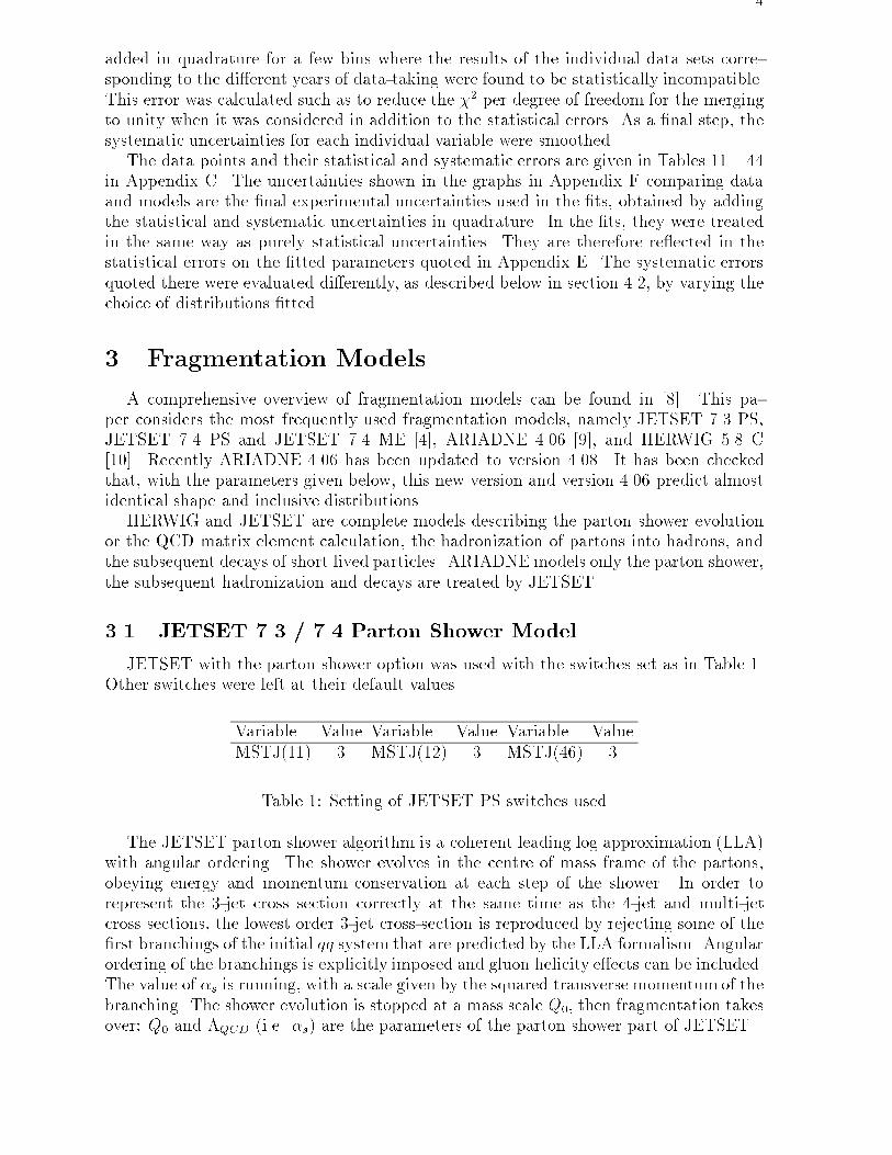
JETSET with the parton shower option was used with the switches set as in Table 1.Other switches were left at their default values.

Variable Value Variable Value Variable ValueMSTJ(11) 3 MSTJ(12) 3 MSTJ(46) 3

Table 1: Setting of JETSET PS switches used

The JETSET parton shower algorithm is a coherent leading log approximation (LLA)with angular ordering. The shower evolves in the centre of mass frame of the partons,obeying energy and momentum conservation at each step of the shower. In order torepresent the 3-jet cross section correctly at the same time as the 4-jet and multi-jetcross sections, the lowest order 3-jet cross-section is reproduced by rejecting some of the�rst branchings of the initial q�q system that are predicted by the LLA formalism. Angularordering of the branchings is explicitly imposed and gluon helicity e�ects can be included.The value of �s is running, with a scale given by the squared transverse momentum of thebranching. The shower evolution is stopped at a mass scale Q0, then fragmentation takesover: Q0 and �QCD (i.e. �s) are the parameters of the parton shower part of JETSET.

5

The fragmentation is performed using the Lund string scheme. This can be formulatedas an iterative procedure. A string stretches between the oppositely coloured quark andantiquark via the gluon colour charges. Two gluons nearby in phase space act like a singlegluon with equal total momentum, so the string model is infrared safe. The longitudinalmomentum fraction z of a hadron is determined using the Lund symmetric fragmentationfunction:

f(z) =(1 � z)

z

a

� exp �b �m

2

t

z

!

where m2

t = m2 + p2t is the transverse mass squared of the hadron, and a and b areparameters of the fragmentation function. In principle b is universal, and a can dependon the quark avour. But for heavy quarks, we use instead the Peterson fragmentationfunction [11]:

f(z) =1

z�1 � 1

z� �q

1�z

�2

with parameter �q being �b or �c, since this gives a better description of heavy quarkfragmentation. The transverse momenta of the hadrons are determined from the ptvalues of their constituent quarks, which in turn are chosen from a tunneling process.This leads to a Gaussian p2t behaviour. The relevant parameter is the standard deviationof this distribution, �q.

The tunneling also determines the quark avour generated in the string breakup,leading to a dependence proportional to exp (�m2

q), and thus to negligible heavy quarkproduction in the fragmentation. Due to the higher mass, even strangeness productionis strongly suppressed: P (u�u) : P (d �d) : P (s�s) = 1 : 1 : s, where s � 0:3. Mesonsare produced according to their quark content in the six multiplets with smallest mass,i.e. in the states: 1S0, 3S1, 1P1, 3P0, 3P1 and 3P2. Contrary to the standard formulationimplemented in JETSET, we have de�ned individual production probabilities P (2s+1Lj)for these multiplets, and also for light, strange, charm and bottom avours. Except for thelight 3P0 multiplet, the probabilities for the P -multiplets are taken to be proportionalto (1 � P (1S0)� P (3S1)) � (2j + 1). In a (2 dimensional) string picture, production ofparticles with non-zero angular momentum (i.e. P -states) is suppressed and expected tobe small (about 10% [12]).

Using additional mass relations, the tunneling mechanism is also applied to baryonproduction (replacing a quark by a di-quark). Parameters related to baryon productionare the relative di-quark production rate P (qq)=P (q), an extra strange di-quark sup-pression [P (us)=P (ud)]= s, and an extra suppression P (qq1)=P (qq0) of spin 1 di-quarksrelative to spin 0 ones leading to s = 3=2 and s = 1=2 baryons. Furthermore, it turnedout to be necessary to include an extra suppression of leading baryons, as implementedin JETSET. However, this extra suppression was not used in heavy quark fragmenta-tion, nor in the simulation of heavy particle decays by fragmentation, because the baryonspectra became too soft and there was too strong a suppression of all heavy baryons.

The parameter related to baryon-meson-baryon production, the so-called `popcorn'parameter, was left at its default value, since experimental determinations of this pa-rameter are not fully conclusive (see [13] and references therein). Furthermore we didnot include simulation of Bose Einstein interference. Although, with properly chosen pa-rameters, the Bose Einstein simulation procedure results in a good representation of thecorrelation functions for identical particles, as well as in a strongly improved descriptionof light meson resonance lineshapes [14,15], the energy momentum rescaling performed inthe current procedure (subroutine LUBOEI) is somewhat unphysical, strongly in uences

6

angular distributions between particles and multi-jet rates, and leads to widely di�erentmodel parameters, some of which also tend to become unphysical. For example, comparethe resulting parameters given in Tables 48 and 49 with the parameters of the DELPHIsimulation (Table 10), which includes Bose Einstein interference.

For the tuning of JETSET 7.3 and ARIADNE 4.06, the description of heavy particledecays, and in particular of their branching fractions, has been modi�ed on the basis ofrecent data. Throughout this paper these modi�ed decays are referred to as `DELPHIdecays'. The modi�cations are similar to those implemented as default in JETSET 7.4.Similar modi�cations, based on earlier data, were already implemented in the JETSET7.3 PS Monte Carlo versions used here for modelling detector e�ects (Appendix B).

3.2 JETSET 7.4 Matrix Element Model

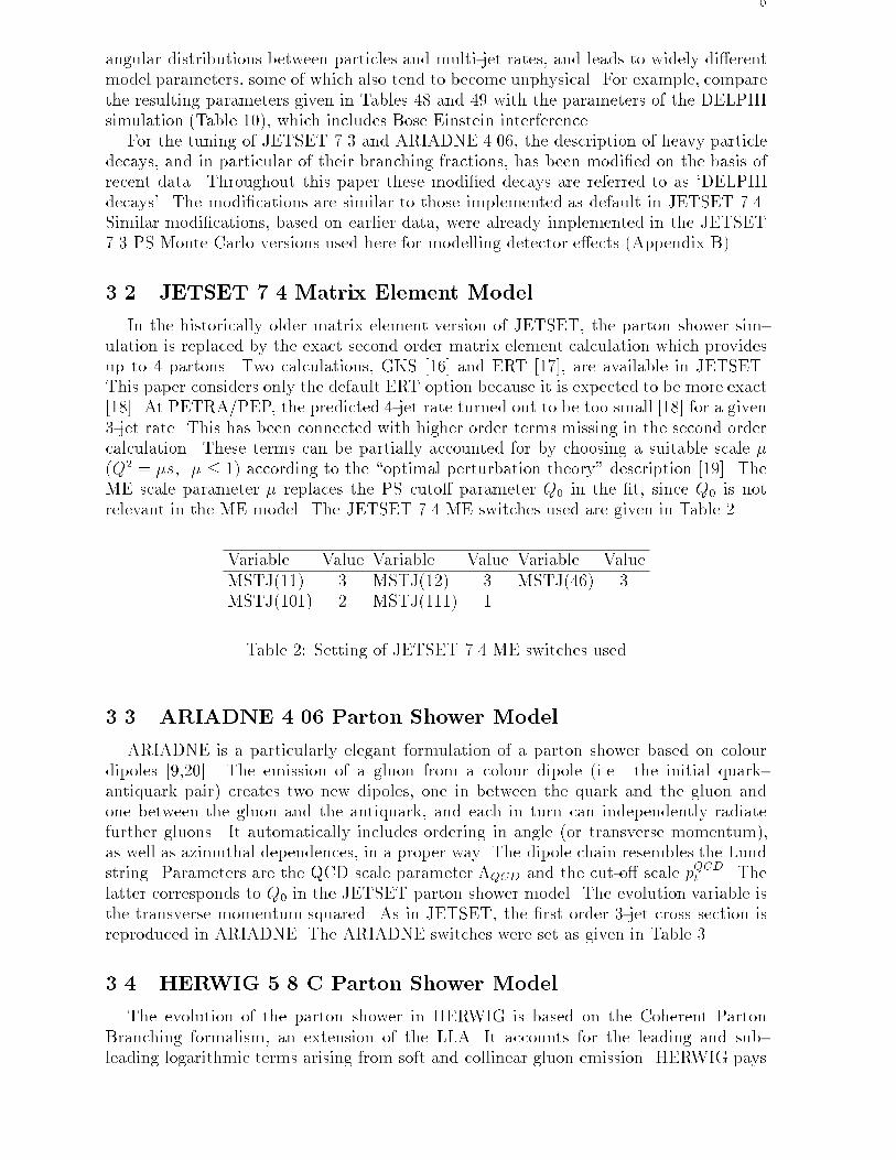
In the historically older matrix element version of JETSET, the parton shower sim-ulation is replaced by the exact second order matrix element calculation which providesup to 4 partons. Two calculations, GKS [16] and ERT [17], are available in JETSET.This paper considers only the default ERT option because it is expected to be more exact[18]. At PETRA/PEP, the predicted 4-jet rate turned out to be too small [18] for a given3-jet rate. This has been connected with higher order terms missing in the second ordercalculation. These terms can be partially accounted for by choosing a suitable scale �(Q2 = �s, � � 1) according to the \optimal perturbation theory" description [19]. TheME scale parameter � replaces the PS cuto� parameter Q0 in the �t, since Q0 is notrelevant in the ME model. The JETSET 7.4 ME switches used are given in Table 2.

Variable Value Variable Value Variable ValueMSTJ(11) 3 MSTJ(12) 3 MSTJ(46) 3MSTJ(101) 2 MSTJ(111) 1

Table 2: Setting of JETSET 7.4 ME switches used

3.3 ARIADNE 4.06 Parton Shower Model

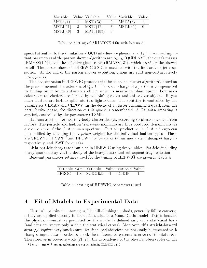
ARIADNE is a particularly elegant formulation of a parton shower based on colourdipoles [9,20]. The emission of a gluon from a colour dipole (i.e. the initial quark-antiquark pair) creates two new dipoles, one in between the quark and the gluon andone between the gluon and the antiquark, and each in turn can independently radiatefurther gluons. It automatically includes ordering in angle (or transverse momentum),as well as azimuthal dependences, in a proper way. The dipole chain resembles the Lundstring. Parameters are the QCD scale parameter �QCD and the cut-o� scale pQCDt . Thelatter corresponds to Q0 in the JETSET parton shower model. The evolution variable isthe transverse momentum squared. As in JETSET, the �rst order 3-jet cross section isreproduced in ARIADNE. The ARIADNE switches were set as given in Table 3.

3.4 HERWIG 5.8 C Parton Shower Model

The evolution of the parton shower in HERWIG is based on the Coherent PartonBranching formalism, an extension of the LLA. It accounts for the leading and sub-leading logarithmic terms arising from soft and collinear gluon emission. HERWIG pays

7

Variable Value Variable Value Variable ValueMSTA(1) 1 MSTA(3) 0 MSTA(5) 1MSTJ(11) 3 MSTJ(12) 3 MSTJ(41) 0MSTJ(46) 3 MSTJ(105) 0

Table 3: Setting of ARIADNE 4.06 switches used

special attention to the simulation of QCD interference phenomena [18]. The most impor-tant parameters of the parton shower algorithm are �QCD (QCDLAM), the quark masses(RMASS(1-6)), and the e�ective gluon mass (RMASS(13)), which provides the showercuto�. The parton shower in HERWIG 5.8 C is matched with the �rst order 3-jet crosssection. At the end of the parton shower evolution, gluons are split non-perturbativelyinto qq-pairs.

The hadronization in HERWIG proceeds via the so-called `cluster algorithm', based onthe precon�nement characteristic of QCD. The colour charge of a parton is compensatedto leading order by an anti-colour object which is nearby in phase space. Low masscolour-neutral clusters are formed by combining colour and anti-colour objects. Highermass clusters are further split into two lighter ones. The splitting is controlled by theparameters CLMAS and CLPOW. In the decay of a cluster containing a quark from theperturbative phase, the direction of this quark is remembered. A Gaussian smearing isapplied, controlled by the parameter CLSMR.

Hadrons are then formed in 2-body cluster decays, according to phase space and spinfactors. The particle and hadron transverse momenta are thus produced dynamically, asa consequence of the cluster mass spectrum. Particle production in cluster decays canbe modi�ed by changing the a priori weights for the individual hadron types. Theseare VECWT, TENWT 2 and DECWT for vector or tensor mesons and decuplet baryonsrespectively, and PWT for quarks.

Light particle decays are simulated in HERWIG using decay tables. Particles includingheavy quarks decay via the decay of the heavy quark and subsequent fragmentation.

Relevant parameter settings used for the tuning of HERWIG are given in Table 4.

Variable Value Variable Value Variable ValueIPROC 100 SUDORD 1 CLDIR 1

Table 4: Setting of HERWIG parameters used

4 Fit of Models to Experimental Data

Classical optimization strategies, like hill-climbing methods, generally fail to convergeif they are applied directly to the optimization of a Monte Carlo model. This is becausethe physical observables predicted by the model is de�ned only on a statistical basis(and thus are known only within the statistical errors). Moreover, this straight-forwardstrategy requires very much computer time, and therefore cannot easily be repeated withchanged input data in order to check the in uence of systematic errors of the data, etc.Therefore, as in previous work [21{23], the dependence of the physical observables on the

2The 1

+�and 0

++meson multiplets are not included in HERWIG 5.8 C.

8

model parameters was approximated analytically. For each bin of each distribution, thequadratic approximation

f(~p0 + �~p; x) = a(0)

0(x) +

nXi=1

a(1)

i (x)�pi +nXi=1

nXj=i

a(2)

ij (x)�pi�pj �MC(~p0 + �~p; x)(1)

was used. In this equation, n is the number of parameters to be �tted, andMC(~p0+�~p; x)denotes the distribution of a physical observable x predicted for a given set of parametervalues ~p0+�~p, where ~p0 is a central parameter setting and �pi is the deviation of parameteri from this setting. The third term in the expansion includes correlation terms betweenthe model parameters. These terms are not present in a linear approximation, such asthat used in [23].

The m = 1 + n + n(n + 1)=2 coe�cients a(0;1;2) of the expansion were determined by�tting Eq. (1) to ` reference simulation distributions (` � m), generated with di�erentparameter settings. This �t is equivalent to solving a system of linear equations:

P � ~a = ~MC (2)

where ~MC is the vector of model predictions corresponding to the parameters ~p0+ �~p(k),

~a is the vector of coe�cients a(k)i(j)(x), and P is a matrix in which column k contains theparameter variations of model set k :

Pk;1::m = ( 1; �p(k)

1 ; :::; �p(k)n ; �p(k)2

1 ; :::; �p(k)2n ; �p(k)

1 � �p(k)2 ; :::; �p(k)

n�1 � �p(k)n )

and k runs from 1 to `. The optimal solution, for an overconstrained linear system(` > m), was obtained using a standard singular value decomposition method [24,25].

The parameters of the ` reference models (generated with equal statistics) were ran-domly chosen in parameter space around the central point ~p0. Assuming the a priori

chosen parameter intervals to be renormalized to �1, it turns out to be unimportant,except for minor di�erences in the statistical precision, whether this volume is a hyper-cube or a hypersphere or whether the points are placed throughout its volume or onits surface. Our choice should ensure that the precision of the �tted linear function isroughly constant within the hypercube.

All simulated sets were generated with equal statistics, large enough that the over-all statistical error was small compared with the experimental uncertainty of the data.Therefore the statistical errors of the simulated data sets have been neglected.

The optimum values of the parameters pi, their errors �i, and their correlation coef-�cients %ij were then determined from a standard �2 �t of the analytic approximation(1) to the corresponding data using MINUIT [26]. The �t was done simultaneously forall distributions and all bins considered. Note that the overall analytic approximation

contains nbins �m coe�cients a(0;1;2)i(j)

(x).In order to minimise the large number of coe�cients to be �tted, if the sensitivity

of a distribution to a given model parameter pi was found to be negligible comparedwith the sensitivity to other parameters (see also next section and Tables 45 - 47 inAppendix D), the dependence of the quadratic expansion (1) on this parameter wassuppressed by omitting it from the linear system (2). This led to a better convergence ofthe minimization and more robust results.

The method was tested by generating `+1 = 51 simulated data sets, with 6 importantfragmentation parameters, and then simultaneously �tting these 6 parameters to each

data set in turn, after using the other 50 data sets to determine the coe�cients a(k)i(j)

(x).

In this case, the statistical error on the coe�cients a(0;1;2)

i(j) (x) of the quadratic expansion

9

(1) was negligible compared with the statistical error of the test set. The pull distributions

(pfiti � ptruei )=�i were found to be approximately standard normal distributions, showingthat the �tting method is self-consistent and unbiased and produces correct errors [14].

4.1 Choice of Distributions

Most parameters of a fragmentation model have a well-de�ned physical meaning. How-ever, some parameters are directly coupled, like a, b, and �q in the Lund fragmentationfunction, while the e�ect of some parameters on physically observed quantities is obscuredby other processes, like decays. Therefore the best choice of distributions for tuning themodel parameters is not always evident. Consequently, from the many possible distri-butions, some have been chosen to determine the central �tted values, and alternativechoices have been used to estimate the systematic uncertainties [7,22,23,27].

In practice, to keep the in uence of statistical errors as small as possible, it is clear thatthe models should be �tted to the distributions that show the strongest dependence onthe parameter under consideration and least dependence on others. For each distributionMC(x), its sensitivity to a given model parameter, i.e. the quantity:

Si(x) =�MC(x)

MC(x)

���pi

.�pipi

� @ lnMC(x)

@ ln jpij���pi

was therefore calculated, where �MC(x) is the change of the distribution MC(x) whenthe model parameter pi is changed by �pi from its central value. Using the fraction �pi=pigives all parameters the same normalization.

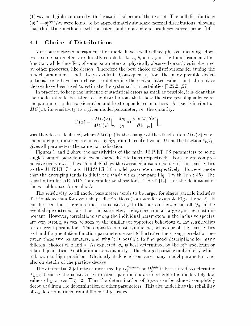
Figures 1 and 2 show the sensitivities of the main JETSET PS parameters to somesingle charged particle and event shape distributions respectively. For a more compre-hensive overview, Tables 45 and 46 show the averaged absolute values of the sensitivitiesto the JETSET 7.4 and HERWIG 5.8 model parameters respectively. However, notethat the averaging tends to dilute the sensitivities (compare Fig. 1 with Table 45). Thesensitivities for ARIADNE are similar to those for JETSET [14]. For the de�nitions ofthe variables, see Appendix A.

The sensitivity to all model parameters tends to be larger for single particle inclusivedistributions than for event shape distributions (compare for example Figs. 1 and 2). Itcan be seen that there is almost no sensitivity to the parton shower cut o� Q0 in theevent shape distributions. For this parameter, the xp spectrum at large xp is the most im-portant. However, correlations among the individual parameters in the inclusive spectraare very strong, as can be seen by the similar (or opposite) behaviour of the sensitivitiesfor di�erent parameters. The opposite, almost symmetric, behaviour of the sensitivitiesto Lund fragmentation function parameters a and b illustrates the strong correlation be-tween these two parameters, and why it is possible to �nd good descriptions for manydi�erent choices of a and b. As expected, �q is best determined by the poutt spectrum orrelated quantities. Another important quantity is the charged particle multiplicity, whichis known to high precision. Obviously it depends on very many model parameters andalso on details of the particle decays.

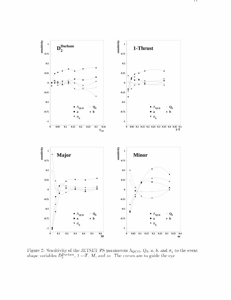
The di�erential 3-jet rate as measured byDDurham2

or DJade2

is best suited to determine�QCD because the sensitivities to other parameters are negligible for moderately lowvalues of ycut, see Fig. 2. Thus the determination of �QCD can be almost completelydecoupled from the determination of other parameters. This also underlines the reliabilityof �s determinations from di�erential jet rates.

10

-1

-0.75

-0.5

-0.25

0

0.25

0.5

0.75

1

0 2 4 6 8 10 12 14 16pt

in

sens

itivi

ty

ptin

ΛQCD Q0

a b

σq

-1

-0.75

-0.5

-0.25

0

0.25

0.5

0.75

1

0 0.5 1 1.5 2 2.5 3 3.5pt

out

sens

itivi

ty

ptout

ΛQCD Q0

a b

σq

-1

-0.75

-0.5

-0.25

0

0.25

0.5

0.75

1

0 0.1 0.2 0.3 0.4 0.5 0.6 0.7 0.8 0.9 1xp

sens

itivi

ty

xp

ΛQCD Q0

a b

σq

Figure 1: Sensitivity of the JETSET PS parameters �QCD, Q0, a, b, and �q to the singleparticle variables pint , p

outt , and xp. The curves are to guide the eye.

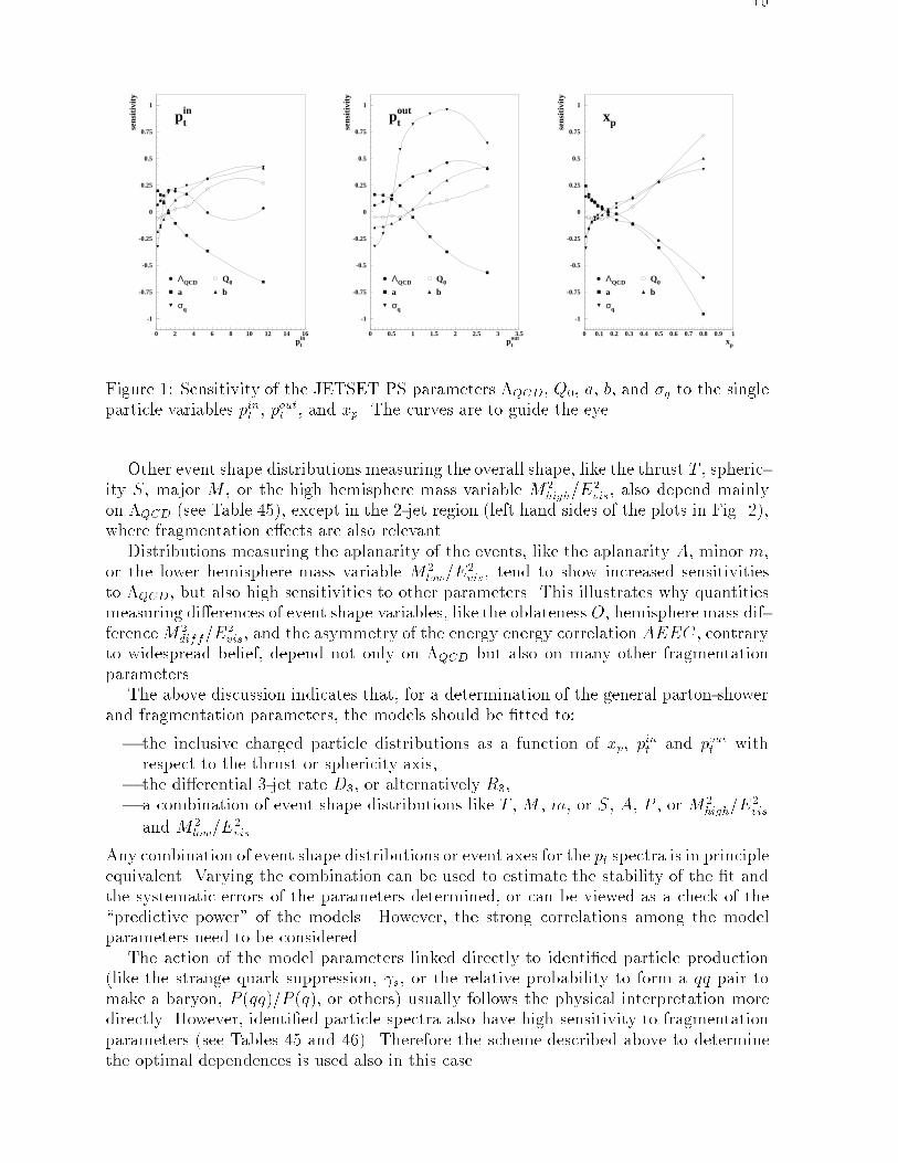
Other event shape distributions measuring the overall shape, like the thrust T , spheric-ity S, major M , or the high hemisphere mass variable M2

high=E2

vis, also depend mainlyon �QCD (see Table 45), except in the 2-jet region (left hand sides of the plots in Fig. 2),where fragmentation e�ects are also relevant.

Distributions measuring the aplanarity of the events, like the aplanarity A, minor m,or the lower hemisphere mass variable M2

low=E2

vis, tend to show increased sensitivitiesto �QCD, but also high sensitivities to other parameters. This illustrates why quantitiesmeasuring di�erences of event shape variables, like the oblateness O, hemisphere mass dif-ferenceM2

diff=E2

vis, and the asymmetry of the energy energy correlation AEEC, contraryto widespread belief, depend not only on �QCD but also on many other fragmentationparameters.

The above discussion indicates that, for a determination of the general parton-showerand fragmentation parameters, the models should be �tted to:

� the inclusive charged particle distributions as a function of xp, pint and poutt withrespect to the thrust or sphericity axis,

� the di�erential 3-jet rate D3, or alternatively R3,� a combination of event shape distributions like T , M , m, or S, A, P , or M2

high=E2

vis

and M2

low=E2

vis.

Any combination of event shape distributions or event axes for the pt spectra is in principleequivalent. Varying the combination can be used to estimate the stability of the �t andthe systematic errors of the parameters determined, or can be viewed as a check of the\predictive power" of the models. However, the strong correlations among the modelparameters need to be considered.

The action of the model parameters linked directly to identi�ed particle production(like the strange quark suppression, s, or the relative probability to form a qq pair tomake a baryon, P (qq)=P (q), or others) usually follows the physical interpretation moredirectly. However, identi�ed particle spectra also have high sensitivity to fragmentationparameters (see Tables 45 and 46). Therefore the scheme described above to determinethe optimal dependences is used also in this case.

11

-1

-0.75

-0.5

-0.25

0

0.25

0.5

0.75

1

0 0.05 0.1 0.15 0.2 0.25 0.3 0.35ycut

sens

itivi

ty

D2Durham

ΛQCD Q0

a b

σq

-1

-0.75

-0.5

-0.25

0

0.25

0.5

0.75

1

0 0.05 0.1 0.15 0.2 0.25 0.3 0.35 0.4 0.45 0.51-T

sens

itivi

ty

1-Thrust

ΛQCD Q0

a b

σq

-1

-0.75

-0.5

-0.25

0

0.25

0.5

0.75

1

0 0.1 0.2 0.3 0.4 0.5 0.6M

sens

itivi

ty

Major

ΛQCD Q0

a b

σq

-1

-0.75

-0.5

-0.25

0

0.25

0.5

0.75

1

0 0.05 0.1 0.15 0.2 0.25 0.3 0.35 0.4m

sens

itivi

ty

Minor

ΛQCD Q0

a b

σq

Figure 2: Sensitivity of the JETSET PS parameters �QCD, Q0, a, b, and �q to the eventshape variables DDurham

2, 1� T , M , and m. The curves are to guide the eye.

12

4.2 Strategy of the Fit

4.2.1 JETSET & ARIADNE

Fits of the general fragmentation parameters (�QCD; Q0 or � or pQCDt ; a, b and �q)were �rst performed to the charged particle inclusive distributions and global event shapedistributions. In order to determine the coe�cients a(0;1;2)(x) in (1), 50 simulated setswith 100000 events each were used for each �t. Parameters related to identi�ed particleswere set to values similar to those used for the DELPHI simulation (see Table 10), sincethese were already known to describe identi�ed particle rates and spectra well.

The average scaled energies < xE > of charm and beauty particles in the modelsdepend only on �c, �b and �QCD. However, the stable hadron spectra depend only weaklyon the heavy quark fragmentation parameters. The following procedure was adopted toreduce further the dependences of the stable particle distributions on the heavy quarkparameters and at the same time to ensure correct < xE > values for D� and B mesons.The < xE > values for D� and B mesons were determined within the model for severalchoices of �QCD and �c(b). Then the dependence of �c(b) on < xE >D�(B) and �QCD

was parametrized. This allowed the method to choose, for each model set and its given�QCD value, corresponding values of �c(b) such that the model set reproduced within theirerrors the average heavy meson scaled momenta as measured by the LEP experiments:< xE >D�= 0:504 � 0:009, < xE >B= 0:701 � 0:008 [28].

The models were then �tted to several combinations of inclusive charged particle andevent shape distributions. The results for �QCD and �q were relatively stable, those for

Q0 or pQCDt less so, and there were many di�erent solutions for a and b, because of the

strong correlation between these two parameters. Therefore only one central value of bwas used in later �ts and only a was treated as a variable. The parameter a was preferredbecause it is less directly coupled to �q in the Lund fragmentation function.

Parameters relevant only to the production of speci�c particles were then adjusted tothe related data. In overview :

� the extra � and �0 suppressions were adjusted to data from [29,30];� the probabilities for producing the di�erent B meson multiplets were adjusted to

agree with recent measurements [31,32] and the corresponding D meson probabilitieswere interpolated between the B and light meson values;

� [P (us)=P (ud)]= s, the strange baryon suppression, was adjusted to the ratio of �0

to proton production [13,33{36];� the leading baryon suppression was adjusted to the high momentumtail of the proton

and �0 spectra [13,33{36];� P (qq1)=P (qq0), the spin 1 di-quark suppression, was adjusted to the ratio of �(1385)

to �0 or proton production [13,33,34,36,37].

Then a simultaneous �t of 10 important parameters (see Tables 48 { 52 in Appendix E)was prepared, by generating 100 simulated data sets of 100000 events each. The analyticalapproximation obtained from these simulated data sets was then �tted to various choicesof inclusive charged particle, event shape, and identi�ed particle distributions.

The inclusive charged particle and event shape distributions measured by DELPHI inthis analysis were used for these �ts in various combinations, as shown in Table 5. Themean charged particle multiplicity at the Z used in the �ts, < Nch >= 20:92� 0:24, wasan average of all available results [38].

The identi�ed particle distributions used included results from all LEP experiments.The combinations chosen are shown in Table 6. They were selected to take into ac-

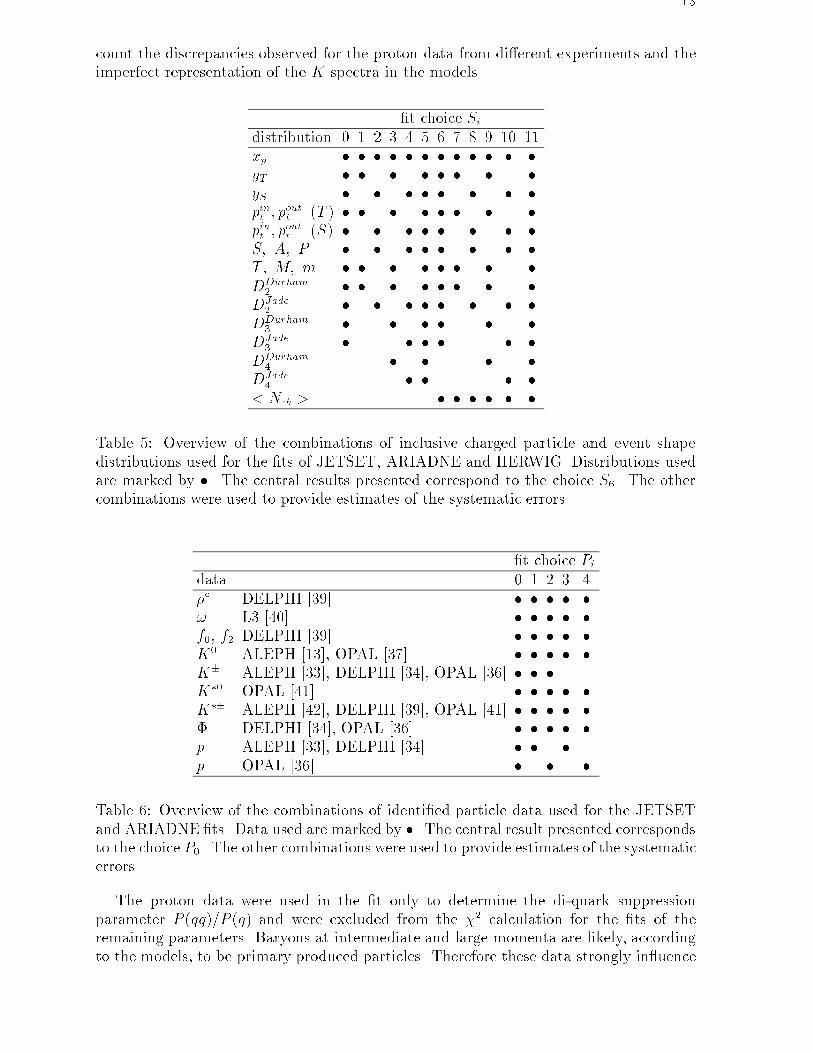
13

count the discrepancies observed for the proton data from di�erent experiments and theimperfect representation of the K spectra in the models.

�t choice Sidistribution 0 1 2 3 4 5 6 7 8 9 10 11xp � � � � � � � � � � � �yT � � � � � � � �yS � � � � � � � �pint ; p

outt (T ) � � � � � � � �

pint ; poutt (S) � � � � � � � �

S; A; P � � � � � � � �T; M; m � � � � � � � �DDurham2

� � � � � � � �DJade2

� � � � � � � �DDurham3

� � � � � �DJade3

� � � � � �DDurham4

� � � �DJade4

� � � �< Nch > � � � � � �

Table 5: Overview of the combinations of inclusive charged particle and event shapedistributions used for the �ts of JETSET, ARIADNE and HERWIG. Distributions usedare marked by �. The central results presented correspond to the choice S6. The othercombinations were used to provide estimates of the systematic errors.

�t choice Pidata 0 1 2 3 4�� DELPHI [39] � � � � �! L3 [40] � � � � �f0, f2 DELPHI [39] � � � � �K0 ALEPH [13], OPAL [37] � � � � �K� ALEPH [33], DELPHI [34], OPAL [36] � � �K�0 OPAL [41] � � � � �K�� ALEPH [42], DELPHI [39], OPAL [41] � � � � �� DELPHI [34], OPAL [36] � � � � �p ALEPH [33], DELPHI [34] � � �p OPAL [36] � � �

Table 6: Overview of the combinations of identi�ed particle data used for the JETSETand ARIADNE �ts. Data used are marked by �. The central result presented correspondsto the choice P0. The other combinations were used to provide estimates of the systematicerrors.

The proton data were used in the �t only to determine the di-quark suppressionparameter P (qq)=P (q) and were excluded from the �2 calculation for the �ts of theremaining parameters. Baryons at intermediate and large momenta are likely, accordingto the models, to be primary produced particles. Therefore these data strongly in uence

14

the primary fragmentation function and the related parameters. Since some experimentaldiscrepancies are present in the proton spectra, and because it had proved necessary tomodify the fragmentation function by an extra suppression at large momenta, this strongimpact on the �t results was considered to be unphysical and therefore was excluded.The �0 data were also excluded from the �nal �ts for similar reasons, and because theyare not described well enough by the models.

Separate �ts were performed for all possible combinations of the 12 choices of inclusiveand event shape distributions in Table 5 with the 5 possible choices of identi�ed particledata in Table 6. A full MINOS [26] error estimate was performed for all parameters.

To check the stability of the �ts, the optimization was started with 6 random startvalues of the fragmentation parameters. The �ts were stable and converged to the samesolution in 95% of cases. The di�erences occurred mainly for two strongly correlatedparameters. Where the �ts gave more than 1 solution, the one with the better �2 waskept.

The central results presented correspond to the combination S6P0. This combinationwas chosen because it contains event shape distributions linear and quadratic in theparticle momenta, the charged particle multiplicity, and all relevant identi�ed particleinformation, so it should result in a complete overall description. The other combinationswere used to provide estimates of the systematic errors. The results are given, with theirstatistical and systematic errors, in Appendix E, Tables 48 { 52.

The results for some of the parameters are strongly correlated. Typical correlationcoe�cients for JETSET 7.4 (default decays) and ARIADNE 4.06 (DELPHI decays) aregiven in Appendix E, Tables 54 and 55. Besides these statistical correlations, furthercorrelations exist due to the di�erent possible choices of input data. The upward (down-ward) systematic error quoted is the root-mean-square spread of the results obtainedfrom all combinations of input data that gave parameter values bigger (smaller) than thecentral �t.

The following observations were made by comparing the results of the di�erent inputdata choices for the JETSET PS �ts.

As should be expected, the results for �QCD, Q0 and �q were almost independent ofthe choice of identi�ed particle data. If just D2 was included in the �t, the resultingvalue of �QCD did not depend on the algorithm used (JADE or DURHAM). However,if the higher jet rates (D3, D4) were included, the �QCD value was somewhat bigger(� 8%) using the JADE algorithm. The values of �QCD and Q0 were positively correlated,implying that the number of �nal partons is more stable within the models than might beexpected from the error of Q0 alone. The parameters �QCD, a and �q were anticorrelated,due to a compensation of the transverse momenta generated in the parton shower andfragmentation phases of the model.

The results for s were higher if the K� data were included as well as the K0 data.P (qq)=P (q) was larger for the ALEPH proton spectrum than for the OPAL one. Pro-duction parameters for strange vector and pseudoscalar mesons were anticorrelated. Ifthe charged particle multiplicity was not included, and therefore the predicted multiplic-ity was smaller than the measured result, the primary production probabilities for lightpseudoscalar and vector mesons were P (1S0)ud � 0:40 and P (3S1)ud � 0:26 respectively.If the multiplicity was �xed to Nch � 20:9, these values were 0.28 and 0.29. This impliessubstantial production probabilities for light p-wave mesons of 0.36 to 0.43.

Most of these observations also apply to ARIADNE. However, in this case the di�erentchoices of D2;D3, etc. led to stable results for �QCD. There was a tendency to obtainslightly bigger values for �QCD from the JADE algorithm (0.245) than from the Durham

15

one (0.237). This is again consistent with the bigger values for pQCDt obtained from JADE(� 0:9 GeV/c) than from DURHAM (� 0:6 GeV/c).

For JETSET ME, �QCD was found to be anticorrelated with the scale �. The frag-mentation parameter values di�er from those from JETSET PS. Especially �q � 0:48GeV/c is much bigger. This partially compensates the missing higher orders in the MEmodel. The values of s and P (qq)=P (q) are smaller than for the PS case and dependless on the choice of input data.

4.2.2 HERWIG

HERWIG uses fewer parameters than JETSET, especially in the hadronization sectorof the model. Therefore a simultaneous �t of all model parameters which are found tobe important is easily performed. These parameters (see Table 46) are:

� the QCD scale parameter QCDLAM and the gluon mass RMASS(13) as majorparameters of the parton shower phase,

� the cluster fragmentation parameters CLMAX, CLPOW, and CLSMR (CLDIR=1),� the a prioriweights PWT(3) for strange quarks, PWT(7) for di-quarks, and DECWT

for decuplet baryons.

Besides the particle spectra, the cluster parameters also strongly in uence the stablecharged particle and event shape distributions. Fits were therefore performed to com-binations of inclusive charged particle and event shape distributions (see Table 5) andidenti�ed particle data (see Table 7). The average scaled momenta of heavy mesons areimportant for the determination of CLMAX and CLPOW.

The identi�ed particle data sets were again chosen (see Table 7) such that systematicdi�erences in the data would be re ected in the systematic errors of the �tted parameters.The central �t result for HERWIG (see Table 53) corresponds to the combination S6P5.The other combinations were used to provide estimates of the systematic errors.

For HERWIG, comparing the results of the di�erent input data choices showed that thevalues obtained for QCDLAM were in general bigger (by � 0:01) when �tting DURHAMrather than JADE jet rates. Contrary to the JETSET case, QCDLAM was smaller (by� 0:005) when the di�erential 2-, 3-, and 4-jet rates were all �tted, rather than the 2-jetrate only. The gluon mass RMASS(13) showed some dependence on the identi�ed particleinformation selected, and on the charged particle multiplicity. The cluster parametersCLMAX and CLPOW depended on the identi�ed particle spectra only when the multi-plicity was not included in the �t. CLPOW was higher for JADE than for DURHAM jetrates. CLSMR depended only on the inclusive charged particle and event shape infor-mation. Including the baryon decuplet data tended to spoil the description of the octetsector.

5 Comparison of Models to Data

The �ts of the individual fragmentation models are compared with corrected DELPHIdata (this analysis) in Figs. 3{38 collected in Appendix F. Figs. 3{32 and 37{38 showdata measured from charged particles only, while Figs. 33{36 compare the models witha few selected distributions measured for charged and neutral particles. All distributionsare corrected to the corresponding �nal states. The lower insets of the plots depict therelative deviation of the models from the data. Also shown, as shaded areas in these

16

�t choice Pidata 0 1 2 3 4 5 6 7 8 9�� DELPHI [39] � � � � � � � � � �! L3 [40] � � � � � � � � � �f2 DELPHI [39] � � � � � � � � � �K0 ALEPH [13], OPAL [37] � � � � � � � � � �K� ALEPH [33], DELPHI [34], OPAL [36] � � � � � �K�0 OPAL [36] � � � � � � � � � �K�� ALEPH [42], DELPHI [39], OPAL [41] � � � � � � � � � �� DELPHI [34], OPAL [36] � � � � � � � � � ��0 ALEPH [13], DELPHI [35] � � � � � ��0 OPAL [41] � � � � � �p ALEPH [33], DELPHI [34] � � � � � �p OPAL [36] � � � � � �� ALEPH [30] � � � � � � � � � ��' ALEPH [30] � � � � � � � � � �< xE > D��;D�0 LEP average [28] � � � � � � � � � �< xE > B0; B� LEP average [28] � � � � � � � � � ���(1385) DELPHI [35], OPAL [41] � � � � ��� DELPHI [35], OPAL [41] � � � � ��0(1530) DELPHI [35], OPAL [41] � � � � �

Table 7: Overview of the combinations of identi�ed particle data used for the HERWIG�ts. Data used are marked by �. The central �t result corresponds to the choice P5. Theother combinations were used to provide estimates of the systematic errors.

insets, are the total experimental errors obtained by adding quadratically the systematicand statistical error in each bin.

The di�erent decay treatments lead to negligible di�erences for the stable chargedparticle and event shape distributions. Comparisons are made with the following models:

� JETSET 7.3 with DELPHI decays labeled JT 7.3 PS� JETSET 7.4 default decays labeled JT 7.4 PS� ARIADNE 4.06 with DELPHI decays labeled AR 4.06� HERWIG 5.8 C default decays labeled H 5.8 C� JETSET 7.4 ME default decays labeled JT 7.4 ME

The observations below are made from the model to data comparisons.

5.1 Inclusive Charged Particle Spectra

All models describe the general trends of the data well. Few discrepancies show upfrom direct model to data comparisons. More quantitatively, the comparisons of modeland data (lower insets) show the following.

The xp spectrum (Fig. 4) for xp < 0:4 is almost perfectly described by the ARIADNEand JETSET PS models. At large xp these models slightly underestimate the data. Thistrend is reduced if the multiplicity is left free in the �t. The HERWIG and JETSET MEpredictions alternate between being too high and too low with respect to the data. Thisbehaviour is also re ected in the rapidity distributions (see Figs. 5, 6).

17

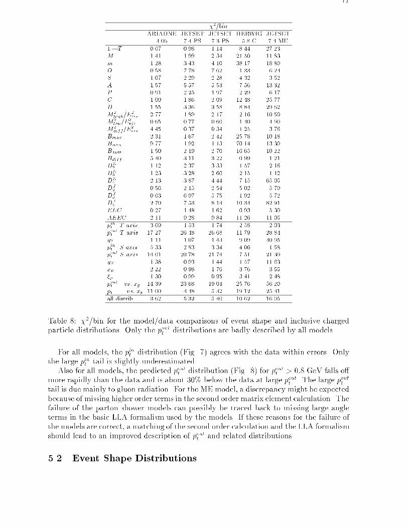
�2=bin

ARIADNE JETSET JETSET HERWIG JETSET4.06 7.4 PS 7.3 PS 5.8 C 7.4 ME

1� T 0.67 0.98 1.14 8.44 27.23M 1.41 1.99 2.34 21.50 11.83m 1.28 3.43 4.10 38.17 18.89O 0.58 7.78 7.62 1.33 6.24S 1.07 2.29 2.28 4.32 3.52A 1.57 5.57 5.53 7.56 13.32P 0.91 2.25 1.97 2.29 6.17C 1.00 1.86 2.09 12.48 25.77D 1.55 3.36 3.58 8.84 29.62M2

high=E2vis 2.77 1.89 2.17 2.16 10.50

M2low=E

2vis 0.65 0.77 0.60 1.40 4.90

M2diff=E

2vis 4.45 0.37 0.34 1.25 3.76

Bmax 2.31 1.67 2.42 25.78 10.18Bmin 9.77 1.92 1.13 70.14 13.39Bsum 1.50 2.19 2.70 16.65 10.22Bdiff: 5.40 3.11 3.22 0.99 1.21DD

2 1.12 2.37 3.33 1.57 2.16DD

3 1.23 3.28 2.60 2.15 1.12DD

4 2.13 3.87 4.44 7.15 65.05DJ

2 0.56 2.15 2.54 5.02 5.79DJ

3 0.63 6.97 5.75 1.92 5.72DJ

4 2.70 7.53 8.13 10.34 82.91EEC 0.27 1.48 1.62 0.93 5.39AEEC 2.11 9.28 9.84 11.26 11.05pint T axis 3.69 1.53 1.74 2.58 2.03poutt T axis 17.27 26.48 26.68 11.79 28.84yT 1.11 1.07 1.43 9.09 40.95pint S axis 5.33 2.83 3.34 4.06 1.58poutt S axis 14.01 20.78 21.74 7.51 21.39yS 1.38 0.93 1.44 1.57 11.63xp 2.22 0.98 1.76 3.76 3.55�p 1.30 0.99 0.95 3.41 2.48poutt vs: xp 14.39 23.68 19.04 25.76 56.20pt vs: xp 11.00 4.48 5.32 19.12 25.41all distrib. 3.62 5.32 5.40 10.62 16.05

Table 8: �2/bin for the model/data comparisons of event shape and inclusive chargedparticle distributions. Only the poutt distributions are badly described by all models.

For all models, the pint distribution (Fig. 7) agrees with the data within errors. Onlythe large pint tail is slightly underestimated.

Also for all models, the predicted poutt distribution (Fig. 8) for poutt > 0:8 GeV falls o�more rapidly than the data and is about 30% below the data at large poutt . The large poutt

tail is due mainly to gluon radiation. For the ME model, a discrepancy might be expectedbecause of missing higher order terms in the second order matrix element calculation. Thefailure of the parton shower models can possibly be traced back to missing large angleterms in the basic LLA formalism used by the models. If these reasons for the failure ofthe models are correct, a matching of the second order calculation and the LLA formalismshould lead to an improved description of poutt and related distributions.

5.2 Event Shape Distributions

18

The general event shape distributions, 1 � T , S, C and Bsum (Figs. 11, 21, 31 and29), are well described within the small experimental errors (typically 2-3%) by all theparton shower models. The HERWIG predictions tend to lie slightly above the data forlarge values of these observables, the JETSET ME predictions tend to oscillate aroundthe data.

The description of distributions sensitive to transverse momenta in the event plane,likeM , Bmax or M2

h=E2

vis (Figs. 12, 27 or 25), is only slightly less good (typically betterthan 5%).

Turning to distributions sensitive to transverse momenta out of the event plane, namelym, O, A,M2

l =E2

vis, and Bmin (Figs. 13, 14, 22, 26, 28), the following pattern is observed:ARIADNE generally describes the data well, while for higher values of the observables,HERWIG tends to overestimate the distributions and JETSET PS to underestimatethem. The latter is to be expected from the underestimation of the poutt distribution byall PS models.

A similar pattern is also observed for the jet rates. The di�erential 2-jet rate D2

(Figs. 15, 16) is well described by all models. ARIADNE describes also the higher jetrates well (Figs. 17{20), HERWIG overestimates and JETSET PS underestimates them.This behaviour is similar for the JADE and DURHAM jet algorithms.

The event shape distributions are less well described by the JETSET ME model thanby the PS models. The extreme 2-jet region, the multi-jet rates, and observables sensitiveto radiation out of the event plane are also not described quite so well. Nevertheless, ingeneral, the description by the JETSET ME model is reasonable.

To permit a comprehensive comparison of the di�erent models, Table 8 shows themean �2/bin obtained from the comparison of the individual data and model distribu-tions. The �2/bin values shown should be used only for relative comparison, not to inferabsolute con�dence levels. In the limit of large statistics, even a slightly imperfect modeldescription leads to a very large �2/bin. Furthermore, in principle, correlations betweenthe di�erent distributions should be taken into account.

5.3 Identi�ed Particle Rates

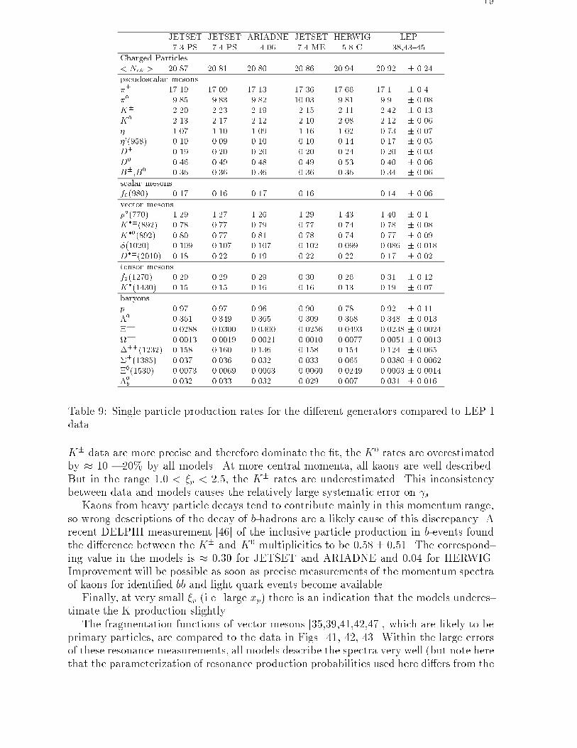
Table 9 compares the particle rates predicted by the models with the current measuredLEP averages. If the mean charged multiplicity < Nch > is included in the �ts, it iswell described by the models. Neglecting this constraint, the multiplicity predicted byARIADNE and JETSET PS is too low (20.2 { 20.4) and that predicted by JETSET MEis too high (22.7). The HERWIG prediction is correct without constraint.

The meson rates, with the exception of the K� and the � rates, are described fairlywell. The K� rate is sensitive to heavy quark decays (see below). The octet baryons alsoagree reasonably. Only HERWIG overestimates the �� rate by about a factor 2. But itgives the best prediction for the � rate. There are some discrepancies in the decupletbaryon sector.

5.4 Meson Momentum Spectra

Figs. 39, 40 compare the models to the identi�ed kaon spectra [13,33{37] as a functionof �p = log 1

xpfrom di�erent LEP experiments. For a more quantitative comparison which

also allows the agreement among the di�erent experiments to be judged, the relativedeviation between the individual data sets and each model is shown by the lines in the�gures on the right. In the fragmentation region at large �p (i.e. small xp), where the

19

JETSET JETSET ARIADNE JETSET HERWIG LEP7.3 PS 7.4 PS 4.06 7.4 ME 5.8 C [38,43{45]

Charged Particles< Nch > 20.87 20.81 20.80 20.86 20.94 20.92 � 0.24pseudoscalar mesons�� 17.19 17.09 17.13 17.36 17.66 17.1 � 0.4�0 9.85 9.83 9.82 10.03 9.81 9.9 � 0.08K� 2.20 2.23 2.19 2.15 2.11 2.42 � 0.13K0 2.13 2.17 2.12 2.10 2.08 2.12 � 0.06� 1.07 1.10 1.09 1.16 1.02 0.73 � 0.07�'(958) 0.10 0.09 0.10 0.10 0.14 0.17 � 0.05D+ 0.19 0.20 0.20 0.20 0.24 0.20 � 0.03D0 0.46 0.49 0.48 0.49 0.53 0.40 � 0.06B�,B0 0.36 0.36 0.36 0.36 0.36 0.34 � 0.06

scalar mesonsf0(980) 0.17 0.16 0.17 0.16 0.14 � 0.06

vector mesons��(770) 1.29 1.27 1.26 1.29 1.43 1.40 � 0.1K��(892) 0.78 0.77 0.79 0.77 0.74 0.78 � 0.08K�0(892) 0.80 0.77 0.81 0.78 0.74 0.77 � 0.09�(1020) 0.109 0.107 0.107 0.102 0.099 0.086 � 0.018D��(2010) 0.18 0.22 0.19 0.22 0.22 0.17 � 0.02tensor mesonsf2(1270) 0.29 0.29 0.29 0.30 0.26 0.31 � 0.12K�(1430) 0.15 0.15 0.16 0.16 0.13 0.19 � 0.07baryonsp 0.97 0.97 0.96 0.90 0.78 0.92 � 0.11�0 0.361 0.349 0.365 0.309 0.368 0.348 � 0.013�� 0.0288 0.0300 0.0300 0.0256 0.0493 0.0238 � 0.0024� 0.0013 0.0019 0.0021 0.0010 0.0077 0.0051 � 0.0013�++(1232) 0.158 0.160 0.136 0.158 0.154 0.124 � 0.065��(1385) 0.037 0.036 0.032 0.033 0.065 0.0380 � 0.0062�0(1530) 0.0073 0.0069 0.0063 0.0060 0.0249 0.0063 � 0.0014�0b 0.032 0.033 0.032 0.029 0.007 0.031 � 0.016

Table 9: Single particle production rates for the di�erent generators compared to LEP Idata.

K� data are more precise and therefore dominate the �t, the K0 rates are overestimatedby � 10 � 20% by all models. At more central momenta, all kaons are well described.But in the range 1:0 < �p < 2:5, the K� rates are underestimated. This inconsistencybetween data and models causes the relatively large systematic error on s.

Kaons from heavy particle decays tend to contribute mainly in this momentum range,so wrong descriptions of the decay of b-hadrons are a likely cause of this discrepancy. Arecent DELPHI measurement [46] of the inclusive particle production in b-events foundthe di�erence between the K� and K0 multiplicities to be 0:58 � 0:51. The correspond-ing value in the models is � 0:30 for JETSET and ARIADNE and 0:04 for HERWIG.Improvement will be possible as soon as precise measurements of the momentum spectraof kaons for identi�ed b�b and light quark events become available.

Finally, at very small �p (i.e. large xp) there is an indication that the models underes-timate the K production slightly.

The fragmentation functions of vector mesons [35,39,41,42,47], which are likely to beprimary particles, are compared to the data in Figs. 41, 42, 43. Within the large errorsof these resonance measurements, all models describe the spectra very well (but note herethat the parameterization of resonance production probabilities used here di�ers from the

20

JETSET default, see section 3). There is only a tendency to predict a somewhat harderfragmentation than measured. This is most evident for the �(1020) spectrum.

Fig. 44 shows good agreement of the model predictions with the measurements ofthe f0(980) scalar and f2(1270) tensor meson [39]. With large production probabilitiesfor p-wave resonances, all models describe the data well. Note that high production ofp-wave states (> 10%) is not expected in the string picture [12].

5.5 Baryon Momentum Spectra

The proton spectra are compared in Fig. 45 [33,34,36]. There is a severe discrepancybetween the OPAL and ALEPH results at small �p. Since both data sets are used for thecentral �ts, the �ts interpolate between them.

For both data sets, the rate predicted by HERWIG is too high at small �p and toolow at high �p. At small �p, i.e. high momentum, the behaviour of JETSET PS andARIADNE is similar to that of HERWIG if the extra baryon suppression is not used.The need for an extra suppression of high momentum baryon production may indicate adi�erent production mechanism for baryons than for mesons. It could also be partly dueto orbitally excited states missing in the models [8]. However, these states have not yetbeen observed in e+e� annihilation.

The experimental situation for the �0 spectrum [13,35,48] also shows some discrepan-cies (see Fig. 46). JETSET PS and ARIADNE describe or slightly overestimate the small�p region. The HERWIG prediction is again too high. At large �p, where the measure-ments agree, all models underestimate the �0 production by � 15%. Better descriptionsmay be obtainable by restricting to the proton and �0 spectra of speci�ed experimentsor by �tting all parameters relevant to baryon production simultaneously [50].

Fig. 47 shows in a comprehensive overview a comparison of the octet and decupletbaryon production [13,35,48,49] with the model predictions. The discrepancies discussedabove are hidden here, due to the large scales. JETSET and ARIADNE describe the grossfeatures of the octet and decuplet baryon production well. HERWIG predicts too harda baryon fragmentation, and also predicts the relative production rates of the di�erentmultiplet states less well.

6 Summary

Precise fully corrected inclusive charged particle and event shape distributions havebeen determined from 750000 e+e� ! Z ! hadrons events measured by the DELPHIexperiment.

A systematic quantitative study has been undertaken to determine the optimal choiceof distributions to tune fragmentation models. Semi-inclusive charged particle and iden-ti�ed particle distributions constrain the hadronization part of the models, whereas 3-jetrate distributions and most event shape distributions mainly control the parton showerparameters (especially �QCD) in the models.

Optimum parameter values have been determined for the ARIADNE 4.06, HERWIG5.8 C and JETSET 7.3 and 7.4 parton shower models and for the JETSET 7.4 matrixelement model. The models were �tted to the event shape and inclusive charged particledistributions measured in this analysis and to the mean charged particle multiplicity andidenti�ed particle data measured by all the LEP experiments. The �t algorithm employedallowed a simultaneous �t of up to 10 model parameters. Statistical and systematic errorsas well as correlations of the model parameters have been determined.

21

All models describe the inclusive charged particle and event shape distributions reason-ably well. The data measured from charged particles and charged plus neutral particlesyield consistent results when compared with the corresponding model predictions. Allmodels underestimate the tail of the poutt distribution by more than 25%. With thisexception, the best overall description is provided by ARIADNE 4.06. HERWIG 5.8 Ctends to overestimate and JETSET 7.3/7.4 to underestimate the production of 4 or morejet events. The tails of event shape distributions sensitive to particle production out ofthe event plane are overestimated (underestimated) by HERWIG (JETSET). The matrixelement model JETSET 7.4 ME with optimized scale also provides reasonable predic-tions. However, it shows the expected discrepancies in the extreme 2-jet and multi-jetregions due to the missing higher order terms.

Identi�ed meson spectra are fairly well described by all models. It has been foundthat strong production of p-wave resonances (25�40%) has to be considered. This is notexpected in a string fragmentation picture. The gross features of baryon production aredescribed by JETSET and ARIADNE. HERWIG shows stronger discrepancies, with thepredicted fragmentation functions being too hard. In JETSET and ARIADNE, a similartendency has been corrected by applying an extra leading baryon suppression.

Acknowledgements

We are greatly indebted to our technical collaborators and to the funding agenciesfor their support in building and operating the DELPHI detector, and to the CERN-SLDivision for the superb performance of the LEP collider. We would like to thank G.Heindl, I. Knowles, L. L�onnblad, M. Seymour and T. Sj�ostrand for useful discussions.

22

A De�nition of Variables

This paper uses the following de�nitions of event shape and inclusive particle variables:

A.1 Inclusive Single Particle Variables

Scaled Momentum, xp, �pThe scaled momentum, xp, is the absolute momentum, j~pj, of aparticle scaled to the beam momentum, while �p = log 1

xp.

Transverse Momenta, pt, pint ; p

outt

With respect to the thrust axis, the component of the transversemomentum pt of a particle in the event plane is pint = ~p�~nMajor andthat out of the event plane is poutt = ~p �~nMinor. For the values withrespect to the sphericity axis, the axes de�ned by the eigenvectorsof the quadratic momentum tensor are used instead.

Rapidity y

The rapidity is given by:

y =1

2� log E + pk

E � pk

where pk is the particle momentum parallel to the event thrustaxis ~nThrust for yT , or the sphericity axis ~nSphericity for yS.

A.2 Event Shape Variables

Thrust T , Major M , Minor m, Oblateness O

The Thrust [51], T , and the Thrust axis, ~nThrust, are de�ned by:

T = max~nThrust

NparticlePi=1

j~pi � ~nThrustjNparticleP

i=1

j~pij

~nThrust is a unit-vector along the Thrust axis. Major and Minorare de�ned similarly, replacing ~nThrust by ~nMajor, perpendicular to~nThrust, and ~nMinor = ~nMajor � ~nThrust respectively. The Oblate-ness is O =M �m.

Sphericity S, Aplanarity A, Planarity P

Ordering the eigenvalues � of the quadratic momentum tensor:

M�� =NparticleX

i=1

p�i p�i (�; � = 1; 2; 3)

�1 � �2 � �3 �1 + �2 + �3 = 1

The Sphericity is S = 3

2(�2 + �3), the Aplanarity is A = 3

2�3,

and the Planarity is P = 2

3(S � 2A) [52]. The Sphericity axis is

parallel to the eigenvector corresponding to �1. As the momentaenter quadratically, the Sphericity axis is in uenced more stronglyby large momentum particles than the Thrust axis.

23

C and D Parameters

The C and D Parameters are de�ned through the eigenvalues � ofthe linear momentum tensor [53]:

�i;j =1

NparticlePk=1

j~pkj�NparticleXk=1

pikpjk

j~pkj

C = 3 � (�1�2 + �2�3 + �3�1) D = 27 � �1�2�3Hemisphere Masses M2

high=E2

vis;M2

low=E2

vis;M2

diff=E2

vis (also called Jet Masses)

Particles are ordered in the two hemispheres of an event separatedby the plane normal to ~nThrust. Then

M2

high

E2

vis

=1

E2

vis

�max

0B@0@ X~pk�~nThrust>0

pk

1A2

;

0@ X~pk�~nThrust<0

pk

1A21CA

ForM2low

E2vis

the maximum in the above formula is replaced by the

minimum, andM2diff

E2vis

=M2high

E2vis

� M2low

E2vis

. This de�nition di�ers from

the original one by Clavelli [54], but is easier to calculate andtherefore preferred by many experiments.

Hemisphere Broadening Bmax; Bmin; Bsum; Bdiff (also called Jet Broadening)

In each hemisphere, de�ned in the same way as for the hemispheremasses, the momenta transverse to the thrust axis are summed anddivided by the corresponding sum of the absolute momenta [55],i.e.

B� =

P�~pi�~nThrust>0

j ~pi � ~nThrust j

2Pi

j~pij

Bmax = max(B+; B�); Bmin = min (B+; B�);

Bsum = B+ +B�; Bdiff = jB+ �B�j:Di�erential Jet Rates Di(y)

Jets are reconstructed using cluster �nding algorithms. For theJADE [56] or Durham [57] algorithm respectively, the scaled in-variant mass or transverse momentum yij :

yJadeij = 2EiEj=E2

vis � (1� cos �ij)

yDurhamij = 2min(E2

i ; E2

j )=E2

vis � (1� cos �ij)

is evaluated for each pair of particles i and j in an event, whereEi, Ej are the energies and �ij the angle between the momentumvectors of the two particles. The particle pair with the lowest valueof yij is replaced by a pseudo-particle with 4-momentum (pi+ pj),reducing the multiplicity by one. The procedure is repeated untilthe scaled invariant masses of all pairs of (pseudo-)particles exceeda given resolution y. The remaining (pseudo-)particles are called

24

jets. The di�erential 2-jet rate D2 is derived from the 2-jet rateR2 = N2�jets=N [58]:

D2(y) =R2(y +�y)�R2(y)

�y

Higher di�erential jet rates follow from the recursion:

Dn(y) =Rn(y +�y)�Rn(y)

�y+Dn�1(y)

Energy-Energy-Correlation EEC and Asymmetry AEEC

The Energy-Energy-Correlation EEC is the histogram of angles,�ij, between all particles weighted by their scaled energies [59]:

EEC(cos�) =1

N

1

�cos��

NXevents

Xi<j

Ei

Evis

Ej

Evis

�(�cos��j cos��cos�ijj)

where cos� and �cos� are the lower edge and width of a binrespectively, and � is the step function. For cos� � 0, the asym-metry AEEC of the EEC is:

AEEC(cos�) = EEC(� cos�)�EEC(cos�)

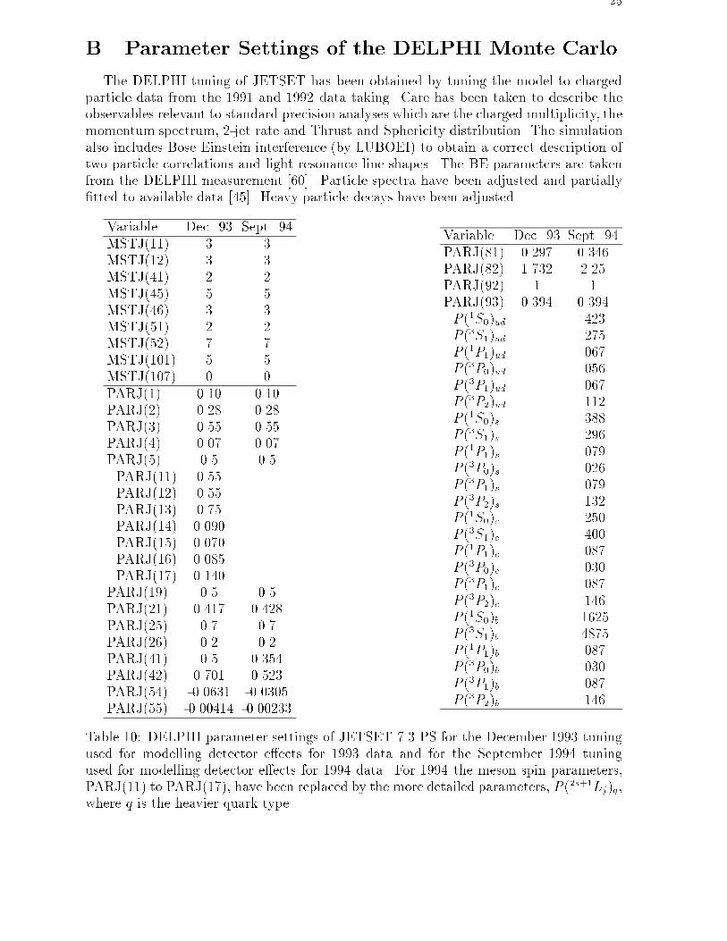
25

B Parameter Settings of the DELPHI Monte Carlo

The DELPHI tuning of JETSET has been obtained by tuning the model to chargedparticle data from the 1991 and 1992 data taking. Care has been taken to describe theobservables relevant to standard precision analyses which are the charged multiplicity, themomentum spectrum, 2-jet rate and Thrust and Sphericity distribution. The simulationalso includes Bose Einstein interference (by LUBOEI) to obtain a correct description oftwo particle correlations and light resonance line shapes. The BE parameters are takenfrom the DELPHI measurement [60]. Particle spectra have been adjusted and partially�tted to available data [45]. Heavy particle decays have been adjusted.

Variable Dec. 93 Sept. 94MSTJ(11) 3 3MSTJ(12) 3 3MSTJ(41) 2 2MSTJ(45) 5 5MSTJ(46) 3 3MSTJ(51) 2 2MSTJ(52) 7 7MSTJ(101) 5 5MSTJ(107) 0 0PARJ(1) 0.10 0.10PARJ(2) 0.28 0.28PARJ(3) 0.55 0.55PARJ(4) 0.07 0.07PARJ(5) 0.5 0.5PARJ(11) 0.55PARJ(12) 0.55PARJ(13) 0.75PARJ(14) 0.090PARJ(15) 0.070PARJ(16) 0.085PARJ(17) 0.140

PARJ(19) 0.5 0.5PARJ(21) 0.417 0.428PARJ(25) 0.7 0.7PARJ(26) 0.2 0.2PARJ(41) 0.5 0.354PARJ(42) 0.701 0.523PARJ(54) -0.0631 -0.0305PARJ(55) -0.00414 -0.00233

Variable Dec. 93 Sept. 94PARJ(81) 0.297 0.346PARJ(82) 1.732 2.25PARJ(92) 1 1PARJ(93) 0.394 0.394P (1S0)ud .423P (3S1)ud .275P (1P1)ud .067P (3P0)ud .056P (3P1)ud .067P (3P2)ud .112P (1S0)s .388P (3S1)s .296P (1P1)s .079P (3P0)s .026P (3P1)s .079P (3P2)s .132P (1S0)c .250P (3S1)c .400P (1P1)c .087P (3P0)c .030P (3P1)c .087P (3P2)c .146P (1S0)b .1625P (3S1)b .4875P (1P1)b .087P (3P0)b .030P (3P1)b .087P (3P2)b .146

Table 10: DELPHI parameter settings of JETSET 7.3 PS for the December 1993 tuningused for modelling detector e�ects for 1993 data and for the September 1994 tuningused for modelling detector e�ects for 1994 data. For 1994 the meson spin parameters,PARJ(11) to PARJ(17), have been replaced by the more detailed parameters, P (2s+1Lj)q,where q is the heavier quark type.

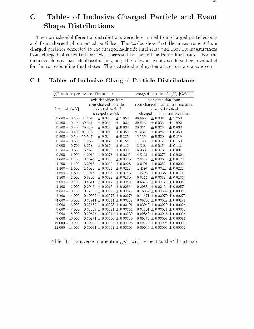
26

C Tables of Inclusive Charged Particle and Event

Shape Distributions

The normalized di�erential distributions were determined from charged particles onlyand from charged plus neutral particles. The tables show �rst the measurement fromcharged particles corrected to the charged hadronic �nal state and then the measurementfrom charged plus neutral particles corrected to the full hadronic �nal state. For theinclusive charged particle distributions, only the relevant event axes have been evaluatedfor the corresponding �nal states. The statistical and systematic errors are also given.

C.1 Tables of Inclusive Charged Particle Distributions

pint with respect to the Thrust axis charged particles 1N

dn

dpint

[GeV�1]

axis de�nition from axis de�nition fromseen charged particles seen charged plus neutral particles

Interval [GeV] corrected to �nal corrected to �nalcharged particles charged plus neutral particles

0.000 - 0.100 44.667 � 0.036 � 1.653 46.663 � 0.037 � 1.7580.100 - 0.200 39.331 � 0.033 � 1.062 39.823 � 0.033 � 1.0920.200 - 0.300 29.429 � 0.028 � 0.603 29.351 � 0.028 � 0.6080.300 - 0.400 21.326 � 0.024 � 0.353 21.034 � 0.024 � 0.3500.400 - 0.500 15.547 � 0.020 � 0.225 15.156 � 0.020 � 0.2190.500 - 0.600 11.463 � 0.017 � 0.156 11.149 � 0.017 � 0.1500.600 - 0.700 8.668 � 0.015 � 0.116 8.348 � 0.015 � 0.1110.700 - 0.800 6.664 � 0.013 � 0.090 6.430 � 0.013 � 0.0870.800 - 1.000 4.6916 � 0.0078 � 0.0646 4.5131 � 0.0076 � 0.06241.000 - 1.200 3.0694 � 0.0063 � 0.0430 2.9522 � 0.0062 � 0.04201.200 - 1.400 2.0913 � 0.0052 � 0.0298 2.0401 � 0.0052 � 0.02991.400 - 1.600 1.5030 � 0.0044 � 0.0218 1.4597 � 0.0044 � 0.02221.600 - 1.800 1.0916 � 0.0038 � 0.0163 1.0796 � 0.0038 � 0.01711.800 - 2.000 0.8306 � 0.0033 � 0.0130 0.8155 � 0.0033 � 0.01362.000 - 2.500 0.5311 � 0.0017 � 0.0089 0.5326 � 0.0017 � 0.00952.500 - 3.000 0.2946 � 0.0013 � 0.0055 0.2988 � 0.0013 � 0.00573.000 - 3.500 0.17405 � 0.00097 � 0.00372 0.18067 � 0.00099 � 0.003833.500 - 4.000 0.10909 � 0.00077 � 0.00276 0.11471 � 0.00079 � 0.002734.000 - 5.000 0.05911 � 0.00041 � 0.00182 0.06305 � 0.00042 � 0.001715.000 - 6.000 0.02669 � 0.00028 � 0.00101 0.03040 � 0.00029 � 0.000956.000 - 7.000 0.01369 � 0.00021 � 0.00064 0.01501 � 0.00021 � 0.000547.000 - 8.000 0.00675 � 0.00014 � 0.00039 0.00858 � 0.00016 � 0.000358.000 - 10.000 0.00271 � 0.00006 � 0.00019 0.00376 � 0.00008 � 0.0001710.000 - 12.000 0.00095 � 0.00004 � 0.00008 0.00123 � 0.00004 � 0.0000612.000 - 14.000 0.00031 � 0.00002 � 0.00003 0.00044 � 0.00003 � 0.00002

Table 11: Transverse momentum, pint , with respect to the Thrust axis

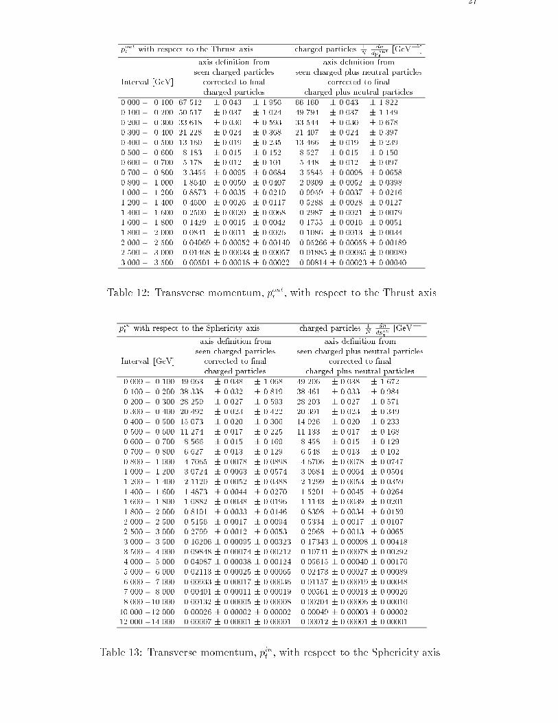
27

poutt with respect to the Thrust axis charged particles 1N

dn

dpoutt

[GeV�1]

axis de�nition from axis de�nition fromseen charged particles seen charged plus neutral particles

Interval [GeV] corrected to �nal corrected to �nalcharged particles charged plus neutral particles

0.000 - 0.100 67.512 � 0.043 � 1.956 66.160 � 0.043 � 1.8220.100 - 0.200 50.517 � 0.037 � 1.024 49.794 � 0.037 � 1.1490.200 - 0.300 33.618 � 0.030 � 0.593 33.544 � 0.030 � 0.6780.300 - 0.400 21.228 � 0.024 � 0.368 21.407 � 0.024 � 0.3970.400 - 0.500 13.160 � 0.019 � 0.235 13.466 � 0.019 � 0.2390.500 - 0.600 8.183 � 0.015 � 0.152 8.527 � 0.015 � 0.1500.600 - 0.700 5.178 � 0.012 � 0.101 5.448 � 0.012 � 0.0970.700 - 0.800 3.3455 � 0.0095 � 0.0684 3.5845 � 0.0098 � 0.06580.800 - 1.000 1.8640 � 0.0050 � 0.0407 2.0309 � 0.0052 � 0.03981.000 - 1.200 0.8873 � 0.0035 � 0.0210 0.9959 � 0.0037 � 0.02161.200 - 1.400 0.4600 � 0.0026 � 0.0117 0.5288 � 0.0028 � 0.01271.400 - 1.600 0.2500 � 0.0020 � 0.0068 0.2987 � 0.0021 � 0.00791.600 - 1.800 0.1429 � 0.0015 � 0.0042 0.1755 � 0.0016 � 0.00511.800 - 2.000 0.0841 � 0.0011 � 0.0026 0.1086 � 0.0013 � 0.00342.000 - 2.500 0.04069 � 0.00052 � 0.00140 0.05266 � 0.00058 � 0.001892.500 - 3.000 0.01468 � 0.00033 � 0.00057 0.01885 � 0.00035 � 0.000803.000 - 3.500 0.00501 � 0.00018 � 0.00022 0.00814 � 0.00023 � 0.00040

Table 12: Transverse momentum, poutt , with respect to the Thrust axis

pint with respect to the Sphericity axis charged particles 1N

dn

dpint

[GeV�1]

axis de�nition from axis de�nition fromseen charged particles seen charged plus neutral particles

Interval [GeV] corrected to �nal corrected to �nalcharged particles charged plus neutral particles

0.000 - 0.100 49.063 � 0.038 � 1.068 49.206 � 0.038 � 1.6720.100 - 0.200 38.338 � 0.032 � 0.819 38.461 � 0.033 � 0.9840.200 - 0.300 28.259 � 0.027 � 0.593 28.203 � 0.027 � 0.5710.300 - 0.400 20.492 � 0.023 � 0.422 20.391 � 0.023 � 0.3490.400 - 0.500 15.073 � 0.020 � 0.306 14.926 � 0.020 � 0.2330.500 - 0.600 11.274 � 0.017 � 0.225 11.133 � 0.017 � 0.1680.600 - 0.700 8.566 � 0.015 � 0.169 8.458 � 0.015 � 0.1290.700 - 0.800 6.627 � 0.013 � 0.129 6.548 � 0.013 � 0.1020.800 - 1.000 4.7065 � 0.0078 � 0.0898 4.6706 � 0.0078 � 0.07471.000 - 1.200 3.0724 � 0.0063 � 0.0574 3.0684 � 0.0064 � 0.05041.200 - 1.400 2.1120 � 0.0052 � 0.0388 2.1299 � 0.0053 � 0.03591.400 - 1.600 1.4873 � 0.0044 � 0.0270 1.5201 � 0.0045 � 0.02641.600 - 1.800 1.0882 � 0.0038 � 0.0196 1.1143 � 0.0039 � 0.02011.800 - 2.000 0.8101 � 0.0033 � 0.0146 0.8398 � 0.0034 � 0.01592.000 - 2.500 0.5156 � 0.0017 � 0.0094 0.5334 � 0.0017 � 0.01072.500 - 3.000 0.2799 � 0.0012 � 0.0053 0.2968 � 0.0013 � 0.00653.000 - 3.500 0.16206 � 0.00095 � 0.00323 0.17343 � 0.00098 � 0.004183.500 - 4.000 0.09848 � 0.00074 � 0.00212 0.10741 � 0.00078 � 0.002924.000 - 5.000 0.04987 � 0.00038 � 0.00124 0.05615 � 0.00040 � 0.001765.000 - 6.000 0.02113 � 0.00025 � 0.00065 0.02473 � 0.00027 � 0.000896.000 - 7.000 0.00933 � 0.00017 � 0.00036 0.01157 � 0.00019 � 0.000487.000 - 8.000 0.00401 � 0.00011 � 0.00019 0.00561 � 0.00013 � 0.000268.000 - 10.000 0.00132 � 0.00005 � 0.00008 0.00204 � 0.00006 � 0.0001010.000 - 12.000 0.00026 � 0.00002 � 0.00002 0.00049 � 0.00003 � 0.0000212.000 - 14.000 0.00007 � 0.00001 � 0.00001 0.00012 � 0.00001 � 0.00001

Table 13: Transverse momentum, pint , with respect to the Sphericity axis

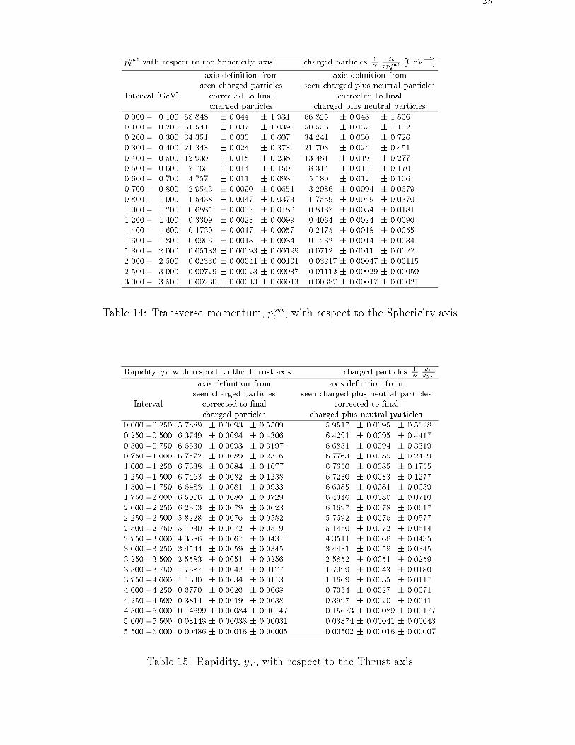
28

poutt with respect to the Sphericity axis charged particles 1N

dn

dpoutt

[GeV�1]

axis de�nition from axis de�nition fromseen charged particles seen charged plus neutral particles

Interval [GeV] corrected to �nal corrected to �nalcharged particles charged plus neutral particles

0.000 - 0.100 68.848 � 0.044 � 1.931 66.825 � 0.043 � 1.5060.100 - 0.200 51.541 � 0.037 � 1.039 50.556 � 0.037 � 1.1020.200 - 0.300 34.351 � 0.030 � 0.607 34.241 � 0.030 � 0.7260.300 - 0.400 21.343 � 0.024 � 0.373 21.708 � 0.024 � 0.4510.400 - 0.500 12.939 � 0.018 � 0.236 13.481 � 0.019 � 0.2770.500 - 0.600 7.765 � 0.014 � 0.150 8.314 � 0.015 � 0.1700.600 - 0.700 4.757 � 0.011 � 0.098 5.180 � 0.012 � 0.1060.700 - 0.800 2.9543 � 0.0090 � 0.0651 3.2986 � 0.0094 � 0.06790.800 - 1.000 1.5438 � 0.0047 � 0.0373 1.7559 � 0.0049 � 0.03701.000 - 1.200 0.6885 � 0.0032 � 0.0186 0.8187 � 0.0034 � 0.01811.200 - 1.400 0.3309 � 0.0023 � 0.0099 0.4064 � 0.0024 � 0.00961.400 - 1.600 0.1730 � 0.0017 � 0.0057 0.2175 � 0.0018 � 0.00551.600 - 1.800 0.0956 � 0.0013 � 0.0034 0.1232 � 0.0014 � 0.00341.800 - 2.000 0.05183 � 0.00093 � 0.00199 0.0712 � 0.0011 � 0.00222.000 - 2.500 0.02330 � 0.00041 � 0.00101 0.03217 � 0.00047 � 0.001152.500 - 3.000 0.00729 � 0.00023 � 0.00037 0.01112 � 0.00029 � 0.000503.000 - 3.500 0.00230 � 0.00013 � 0.00013 0.00387 � 0.00017 � 0.00021

Table 14: Transverse momentum, poutt , with respect to the Sphericity axis

Rapidity yT with respect to the Thrust axis charged particles 1N

dndyT

axis de�nition from axis de�nition fromseen charged particles seen charged plus neutral particles

Interval corrected to �nal corrected to �nalcharged particles charged plus neutral particles

0.000 - 0.250 5.7889 � 0.0093 � 0.5509 5.9517 � 0.0095 � 0.56280.250 - 0.500 6.3749 � 0.0094 � 0.4306 6.4291 � 0.0095 � 0.44170.500 - 0.750 6.6630 � 0.0093 � 0.3197 6.6831 � 0.0094 � 0.33190.750 - 1.000 6.7572 � 0.0089 � 0.2316 6.7763 � 0.0089 � 0.24291.000 - 1.250 6.7638 � 0.0084 � 0.1677 6.7650 � 0.0085 � 0.17551.250 - 1.500 6.7463 � 0.0082 � 0.1238 6.7230 � 0.0083 � 0.12771.500 - 1.750 6.6488 � 0.0081 � 0.0933 6.6085 � 0.0081 � 0.09391.750 - 2.000 6.5006 � 0.0080 � 0.0729 6.4346 � 0.0080 � 0.07102.000 - 2.250 6.2303 � 0.0079 � 0.0623 6.1697 � 0.0078 � 0.06172.250 - 2.500 5.8228 � 0.0076 � 0.0582 5.7692 � 0.0076 � 0.05772.500 - 2.750 5.1930 � 0.0072 � 0.0519 5.1450 � 0.0072 � 0.05142.750 - 3.000 4.3686 � 0.0067 � 0.0437 4.3511 � 0.0066 � 0.04353.000 - 3.250 3.4544 � 0.0059 � 0.0345 3.4481 � 0.0059 � 0.03453.250 - 3.500 2.5583 � 0.0051 � 0.0256 2.5852 � 0.0051 � 0.02593.500 - 3.750 1.7687 � 0.0042 � 0.0177 1.7999 � 0.0043 � 0.01803.750 - 4.000 1.1330 � 0.0034 � 0.0113 1.1669 � 0.0035 � 0.01174.000 - 4.250 0.6770 � 0.0026 � 0.0068 0.7054 � 0.0027 � 0.00714.250 - 4.500 0.3814 � 0.0019 � 0.0038 0.3997 � 0.0020 � 0.00414.500 - 5.000 0.14699 � 0.00084 � 0.00147 0.15673 � 0.00089 � 0.001775.000 - 5.500 0.03148 � 0.00038 � 0.00031 0.03374 � 0.00041 � 0.000435.500 - 6.000 0.00486 � 0.00016 � 0.00005 0.00502 � 0.00016 � 0.00007

Table 15: Rapidity, yT , with respect to the Thrust axis

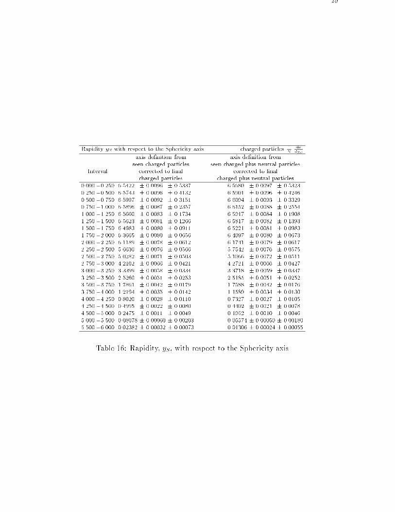
29

Rapidity yS with respect to the Sphericity axis charged particles 1N

dndyS

axis de�nition from axis de�nition fromseen charged particles seen charged plus neutral particles

Interval corrected to �nal corrected to �nalcharged particles charged plus neutral particles

0.000 - 0.250 6.5422 � 0.0096 � 0.5337 6.5680 � 0.0097 � 0.53230.250 - 0.500 6.5743 � 0.0096 � 0.4132 6.5901 � 0.0096 � 0.42460.500 - 0.750 6.5997 � 0.0092 � 0.3151 6.6094 � 0.0093 � 0.33290.750 - 1.000 6.5896 � 0.0087 � 0.2357 6.6152 � 0.0088 � 0.25541.000 - 1.250 6.5660 � 0.0083 � 0.1734 6.5917 � 0.0084 � 0.19081.250 - 1.500 6.5623 � 0.0081 � 0.1266 6.5817 � 0.0082 � 0.13931.500 - 1.750 6.4983 � 0.0080 � 0.0911 6.5221 � 0.0081 � 0.09831.750 - 2.000 6.3665 � 0.0080 � 0.0656 6.4097 � 0.0080 � 0.06732.000 - 2.250 6.1189 � 0.0078 � 0.0612 6.1741 � 0.0079 � 0.06172.250 - 2.500 5.6636 � 0.0076 � 0.0566 5.7542 � 0.0076 � 0.05752.500 - 2.750 5.0282 � 0.0071 � 0.0503 5.1066 � 0.0072 � 0.05112.750 - 3.000 4.2102 � 0.0066 � 0.0421 4.2721 � 0.0066 � 0.04273.000 - 3.250 3.3399 � 0.0058 � 0.0334 3.3718 � 0.0059 � 0.03373.250 - 3.500 2.5260 � 0.0051 � 0.0253 2.5185 � 0.0051 � 0.02523.500 - 3.750 1.7861 � 0.0042 � 0.0179 1.7588 � 0.0042 � 0.01763.750 - 4.000 1.2194 � 0.0035 � 0.0142 1.1589 � 0.0034 � 0.01304.000 - 4.250 0.8020 � 0.0028 � 0.0110 0.7327 � 0.0027 � 0.01054.250 - 4.500 0.4995 � 0.0022 � 0.0080 0.4402 � 0.0021 � 0.00784.500 - 5.000 0.2475 � 0.0011 � 0.0049 0.1952 � 0.0010 � 0.00465.000 - 5.500 0.08078 � 0.00060 � 0.00203 0.05574 � 0.00050 � 0.001805.500 - 6.000 0.02382 � 0.00032 � 0.00073 0.01306 � 0.00024 � 0.00055

Table 16: Rapidity, yS, with respect to the Sphericity axis

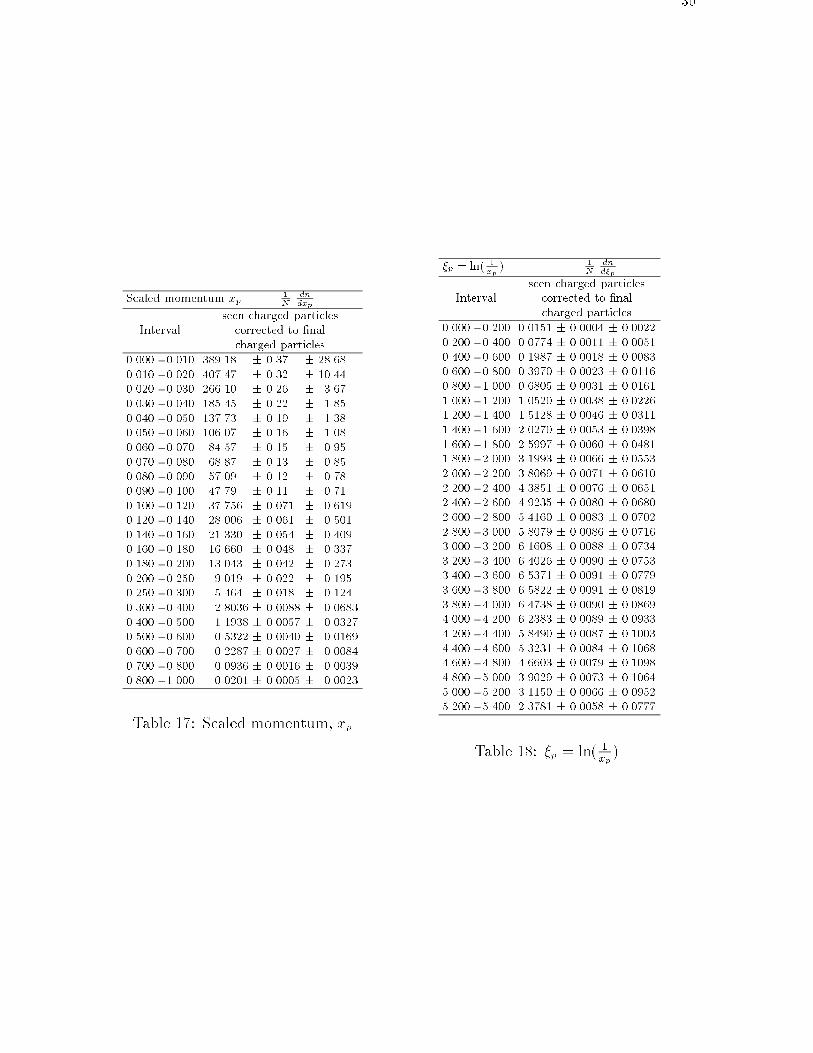
30

Scaled momentum xp1N

dndxp

seen charged particlesInterval corrected to �nal

charged particles0.000 - 0.010 389.18 � 0.37 � 28.680.010 - 0.020 407.47 � 0.32 � 10.440.020 - 0.030 266.10 � 0.26 � 3.670.030 - 0.040 185.45 � 0.22 � 1.850.040 - 0.050 137.73 � 0.19 � 1.380.050 - 0.060 106.07 � 0.16 � 1.080.060 - 0.070 84.57 � 0.15 � 0.950.070 - 0.080 68.87 � 0.13 � 0.850.080 - 0.090 57.09 � 0.12 � 0.780.090 - 0.100 47.79 � 0.11 � 0.710.100 - 0.120 37.756 � 0.071 � 0.6190.120 - 0.140 28.006 � 0.061 � 0.5010.140 - 0.160 21.330 � 0.054 � 0.4090.160 - 0.180 16.660 � 0.048 � 0.3370.180 - 0.200 13.043 � 0.042 � 0.2730.200 - 0.250 9.019 � 0.022 � 0.1950.250 - 0.300 5.464 � 0.018 � 0.1240.300 - 0.400 2.8036 � 0.0088 � 0.06830.400 - 0.500 1.1938 � 0.0057 � 0.03270.500 - 0.600 0.5322 � 0.0040 � 0.01690.600 - 0.700 0.2287 � 0.0027 � 0.00840.700 - 0.800 0.0936 � 0.0016 � 0.00390.800 - 1.000 0.0201 � 0.0005 � 0.0023

Table 17: Scaled momentum, xp

�p = ln( 1xp) 1

Ndnd�p

seen charged particlesInterval corrected to �nal

charged particles0.000 - 0.200 0.0151 � 0.0004 � 0.00220.200 - 0.400 0.0774 � 0.0011 � 0.00510.400 - 0.600 0.1987 � 0.0018 � 0.00830.600 - 0.800 0.3970 � 0.0023 � 0.01160.800 - 1.000 0.6805 � 0.0031 � 0.01611.000 - 1.200 1.0520 � 0.0038 � 0.02261.200 - 1.400 1.5128 � 0.0046 � 0.03111.400 - 1.600 2.0270 � 0.0053 � 0.03981.600 - 1.800 2.5997 � 0.0060 � 0.04811.800 - 2.000 3.1993 � 0.0066 � 0.05532.000 - 2.200 3.8069 � 0.0071 � 0.06102.200 - 2.400 4.3851 � 0.0076 � 0.06512.400 - 2.600 4.9235 � 0.0080 � 0.06802.600 - 2.800 5.4160 � 0.0083 � 0.07022.800 - 3.000 5.8079 � 0.0086 � 0.07163.000 - 3.200 6.1608 � 0.0088 � 0.07343.200 - 3.400 6.4026 � 0.0090 � 0.07533.400 - 3.600 6.5371 � 0.0091 � 0.07793.600 - 3.800 6.5822 � 0.0091 � 0.08193.800 - 4.000 6.4738 � 0.0090 � 0.08694.000 - 4.200 6.2383 � 0.0089 � 0.09334.200 - 4.400 5.8490 � 0.0087 � 0.10034.400 - 4.600 5.3231 � 0.0084 � 0.10684.600 - 4.800 4.6603 � 0.0079 � 0.10984.800 - 5.000 3.9029 � 0.0073 � 0.10645.000 - 5.200 3.1150 � 0.0066 � 0.09525.200 - 5.400 2.3781 � 0.0058 � 0.0777

Table 18: �p = ln( 1

xp)

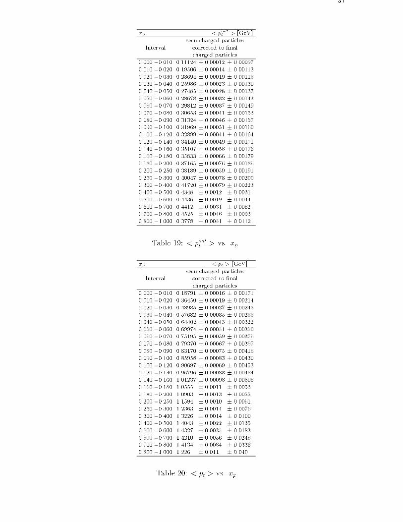
31

xp < poutt > [GeV]seen charged particles

Interval corrected to �nalcharged particles

0.000 - 0.010 0.11124 � 0.00012 � 0.000970.010 - 0.020 0.19506 � 0.00014 � 0.001130.020 - 0.030 0.23694 � 0.00019 � 0.001180.030 - 0.040 0.25986 � 0.00023 � 0.001300.040 - 0.050 0.27485 � 0.00028 � 0.001370.050 - 0.060 0.28678 � 0.00032 � 0.001430.060 - 0.070 0.29812 � 0.00037 � 0.001490.070 - 0.080 0.30653 � 0.00041 � 0.001530.080 - 0.090 0.31324 � 0.00046 � 0.001570.090 - 0.100 0.31969 � 0.00051 � 0.001600.100 - 0.120 0.32899 � 0.00041 � 0.001640.120 - 0.140 0.34140 � 0.00049 � 0.001710.140 - 0.160 0.35107 � 0.00058 � 0.001760.160 - 0.180 0.35833 � 0.00066 � 0.001790.180 - 0.200 0.37165 � 0.00076 � 0.001860.200 - 0.250 0.38189 � 0.00059 � 0.001910.250 - 0.300 0.40047 � 0.00078 � 0.002000.300 - 0.400 0.41720 � 0.00079 � 0.002230.400 - 0.500 0.4348 � 0.0012 � 0.00310.500 - 0.600 0.4436 � 0.0019 � 0.00440.600 - 0.700 0.4412 � 0.0031 � 0.00620.700 - 0.800 0.4525 � 0.0046 � 0.00930.800 - 1.000 0.3778 � 0.0051 � 0.0112

Table 19: < poutt > vs. xp

xp < pt > [GeV]seen charged particles

Interval corrected to �nalcharged particles

0.000 - 0.010 0.18791 � 0.00016 � 0.001710.010 - 0.020 0.36450 � 0.00019 � 0.002140.020 - 0.030 0.48985 � 0.00027 � 0.002450.030 - 0.040 0.57682 � 0.00035 � 0.002880.040 - 0.050 0.64402 � 0.00043 � 0.003220.050 - 0.060 0.69974 � 0.00051 � 0.003500.060 - 0.070 0.75195 � 0.00059 � 0.003760.070 - 0.080 0.79370 � 0.00067 � 0.003970.080 - 0.090 0.83170 � 0.00075 � 0.004160.090 - 0.100 0.85958 � 0.00083 � 0.004300.100 - 0.120 0.90697 � 0.00069 � 0.004530.120 - 0.140 0.96796 � 0.00083 � 0.004840.140 - 0.160 1.01237 � 0.00098 � 0.005060.160 - 0.180 1.0555 � 0.0011 � 0.00530.180 - 0.200 1.0903 � 0.0013 � 0.00550.200 - 0.250 1.1594 � 0.0010 � 0.00610.250 - 0.300 1.2363 � 0.0014 � 0.00760.300 - 0.400 1.3226 � 0.0014 � 0.01000.400 - 0.500 1.4043 � 0.0022 � 0.01350.500 - 0.600 1.4327 � 0.0035 � 0.01830.600 - 0.700 1.4210 � 0.0056 � 0.02460.700 - 0.800 1.4134 � 0.0084 � 0.03360.800 - 1.000 1.226 � 0.011 � 0.040

Table 20: < pt > vs. xp

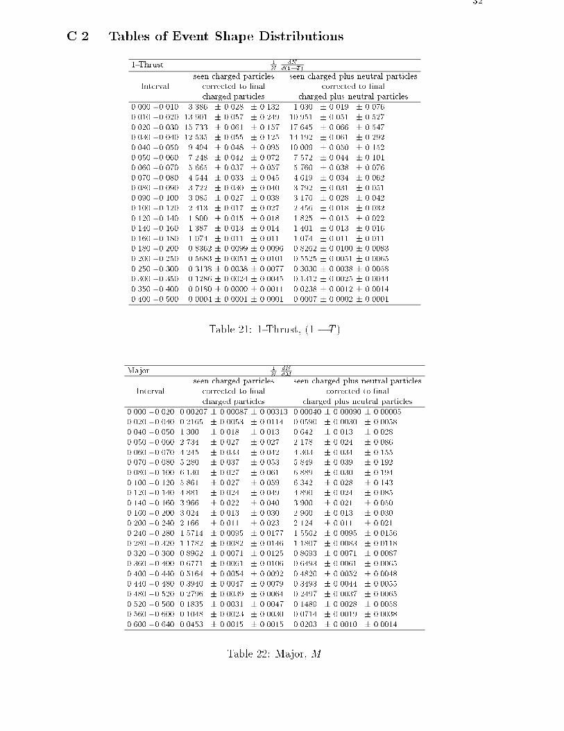
32

C.2 Tables of Event Shape Distributions

1-Thrust 1N

dNd(1�T )

seen charged particles seen charged plus neutral particlesInterval corrected to �nal corrected to �nal

charged particles charged plus neutral particles0.000 - 0.010 3.386 � 0.028 � 0.132 1.030 � 0.019 � 0.0760.010 - 0.020 13.901 � 0.057 � 0.249 10.951 � 0.051 � 0.5270.020 - 0.030 15.733 � 0.061 � 0.157 17.645 � 0.066 � 0.5470.030 - 0.040 12.535 � 0.055 � 0.125 14.192 � 0.061 � 0.2920.040 - 0.050 9.494 � 0.048 � 0.095 10.009 � 0.050 � 0.1520.050 - 0.060 7.248 � 0.042 � 0.072 7.572 � 0.044 � 0.1010.060 - 0.070 5.665 � 0.037 � 0.057 5.760 � 0.038 � 0.0760.070 - 0.080 4.544 � 0.033 � 0.045 4.619 � 0.034 � 0.0620.080 - 0.090 3.722 � 0.030 � 0.040 3.792 � 0.031 � 0.0510.090 - 0.100 3.085 � 0.027 � 0.038 3.176 � 0.028 � 0.0420.100 - 0.120 2.413 � 0.017 � 0.027 2.456 � 0.018 � 0.0320.120 - 0.140 1.800 � 0.015 � 0.018 1.825 � 0.015 � 0.0220.140 - 0.160 1.387 � 0.013 � 0.014 1.401 � 0.013 � 0.0160.160 - 0.180 1.074 � 0.011 � 0.011 1.074 � 0.011 � 0.0110.180 - 0.200 0.8362 � 0.0099 � 0.0096 0.8262 � 0.0100 � 0.00830.200 - 0.250 0.5683 � 0.0051 � 0.0101 0.5525 � 0.0051 � 0.00650.250 - 0.300 0.3138 � 0.0038 � 0.0077 0.3030 � 0.0038 � 0.00580.300 - 0.350 0.1286 � 0.0024 � 0.0045 0.1312 � 0.0025 � 0.00440.350 - 0.400 0.0180 � 0.0009 � 0.0011 0.0238 � 0.0012 � 0.00140.400 - 0.500 0.0004 � 0.0001 � 0.0001 0.0007 � 0.0002 � 0.0001

Table 21: 1-Thrust, (1 � T )

Major 1N

dNdM

seen charged particles seen charged plus neutral particlesInterval corrected to �nal corrected to �nal

charged particles charged plus neutral particles0.000 - 0.020 0.00207 � 0.00087 � 0.00313 0.00040 � 0.00090 � 0.000050.020 - 0.040 0.2165 � 0.0053 � 0.0114 0.0590 � 0.0030 � 0.00580.040 - 0.050 1.300 � 0.018 � 0.013 0.642 � 0.013 � 0.0280.050 - 0.060 2.734 � 0.027 � 0.027 2.178 � 0.024 � 0.0860.060 - 0.070 4.245 � 0.033 � 0.042 4.303 � 0.034 � 0.1550.070 - 0.080 5.280 � 0.037 � 0.053 5.849 � 0.039 � 0.1920.080 - 0.100 6.130 � 0.027 � 0.061 6.889 � 0.030 � 0.1940.100 - 0.120 5.861 � 0.027 � 0.059 6.342 � 0.028 � 0.1430.120 - 0.140 4.881 � 0.024 � 0.049 4.890 � 0.024 � 0.0850.140 - 0.160 3.966 � 0.022 � 0.040 3.900 � 0.021 � 0.0500.160 - 0.200 3.024 � 0.013 � 0.030 2.960 � 0.013 � 0.0300.200 - 0.240 2.166 � 0.011 � 0.023 2.124 � 0.011 � 0.0210.240 - 0.280 1.5714 � 0.0095 � 0.0177 1.5562 � 0.0095 � 0.01560.280 - 0.320 1.1782 � 0.0082 � 0.0146 1.1807 � 0.0083 � 0.01180.320 - 0.360 0.8962 � 0.0071 � 0.0125 0.8693 � 0.0071 � 0.00870.360 - 0.400 0.6771 � 0.0061 � 0.0106 0.6493 � 0.0061 � 0.00650.400 - 0.440 0.5164 � 0.0054 � 0.0092 0.4820 � 0.0052 � 0.00480.440 - 0.480 0.3940 � 0.0047 � 0.0079 0.3493 � 0.0044 � 0.00550.480 - 0.520 0.2796 � 0.0039 � 0.0064 0.2497 � 0.0037 � 0.00650.520 - 0.560 0.1835 � 0.0031 � 0.0047 0.1489 � 0.0028 � 0.00580.560 - 0.600 0.1048 � 0.0023 � 0.0030 0.0714 � 0.0019 � 0.00380.600 - 0.640 0.0453 � 0.0015 � 0.0015 0.0203 � 0.0010 � 0.0014

Table 22: Major, M

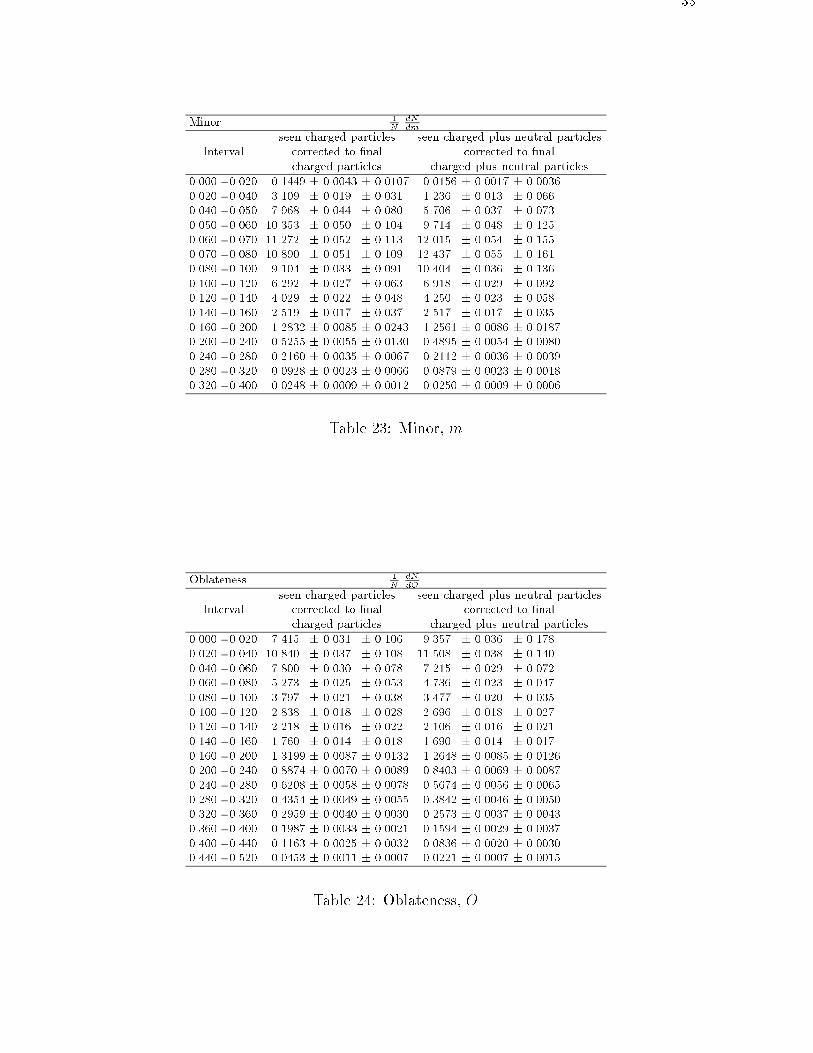
33

Minor 1N

dNdm

seen charged particles seen charged plus neutral particlesInterval corrected to �nal corrected to �nal

charged particles charged plus neutral particles0.000 - 0.020 0.1449 � 0.0043 � 0.0107 0.0156 � 0.0017 � 0.00360.020 - 0.040 3.109 � 0.019 � 0.031 1.236 � 0.013 � 0.0660.040 - 0.050 7.968 � 0.044 � 0.080 5.706 � 0.037 � 0.0730.050 - 0.060 10.353 � 0.050 � 0.104 9.714 � 0.048 � 0.1250.060 - 0.070 11.272 � 0.052 � 0.113 12.015 � 0.054 � 0.1550.070 - 0.080 10.890 � 0.051 � 0.109 12.437 � 0.055 � 0.1610.080 - 0.100 9.104 � 0.033 � 0.091 10.404 � 0.036 � 0.1360.100 - 0.120 6.292 � 0.027 � 0.063 6.918 � 0.029 � 0.0920.120 - 0.140 4.029 � 0.022 � 0.048 4.250 � 0.023 � 0.0580.140 - 0.160 2.519 � 0.017 � 0.037 2.517 � 0.017 � 0.0350.160 - 0.200 1.2832 � 0.0085 � 0.0243 1.2561 � 0.0086 � 0.01870.200 - 0.240 0.5255 � 0.0055 � 0.0130 0.4895 � 0.0054 � 0.00800.240 - 0.280 0.2160 � 0.0035 � 0.0067 0.2112 � 0.0036 � 0.00390.280 - 0.320 0.0928 � 0.0023 � 0.0066 0.0879 � 0.0023 � 0.00180.320 - 0.400 0.0248 � 0.0009 � 0.0012 0.0250 � 0.0009 � 0.0006

Table 23: Minor, m

Oblateness 1N

dNdO

seen charged particles seen charged plus neutral particlesInterval corrected to �nal corrected to �nal

charged particles charged plus neutral particles0.000 - 0.020 7.415 � 0.031 � 0.106 9.357 � 0.036 � 0.1780.020 - 0.040 10.840 � 0.037 � 0.108 11.508 � 0.038 � 0.1400.040 - 0.060 7.800 � 0.030 � 0.078 7.215 � 0.029 � 0.0720.060 - 0.080 5.273 � 0.025 � 0.053 4.736 � 0.023 � 0.0470.080 - 0.100 3.797 � 0.021 � 0.038 3.477 � 0.020 � 0.0350.100 - 0.120 2.838 � 0.018 � 0.028 2.696 � 0.018 � 0.0270.120 - 0.140 2.218 � 0.016 � 0.022 2.106 � 0.016 � 0.0210.140 - 0.160 1.760 � 0.014 � 0.018 1.690 � 0.014 � 0.0170.160 - 0.200 1.3199 � 0.0087 � 0.0132 1.2648 � 0.0085 � 0.01260.200 - 0.240 0.8874 � 0.0070 � 0.0089 0.8403 � 0.0069 � 0.00870.240 - 0.280 0.6208 � 0.0058 � 0.0078 0.5674 � 0.0056 � 0.00650.280 - 0.320 0.4354 � 0.0049 � 0.0055 0.3842 � 0.0046 � 0.00500.320 - 0.360 0.2959 � 0.0040 � 0.0030 0.2573 � 0.0037 � 0.00430.360 - 0.400 0.1987 � 0.0033 � 0.0021 0.1594 � 0.0029 � 0.00370.400 - 0.440 0.1163 � 0.0025 � 0.0032 0.0836 � 0.0020 � 0.00300.440 - 0.520 0.0453 � 0.0011 � 0.0007 0.0221 � 0.0007 � 0.0015

Table 24: Oblateness, O

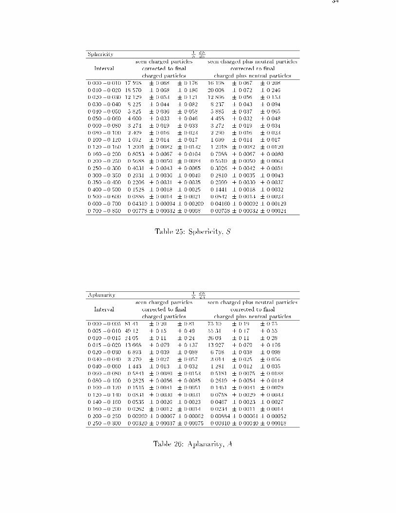
34

Sphericity 1N

dNdS

seen charged particles seen charged plus neutral particlesInterval corrected to �nal corrected to �nal

charged particles charged plus neutral particles0.000 - 0.010 17.598 � 0.068 � 0.176 16.198 � 0.067 � 0.2080.010 - 0.020 18.570 � 0.068 � 0.186 20.008 � 0.072 � 0.2460.020 - 0.030 12.129 � 0.053 � 0.121 12.896 � 0.056 � 0.1530.030 - 0.040 8.225 � 0.044 � 0.082 8.237 � 0.043 � 0.0940.040 - 0.050 5.825 � 0.036 � 0.058 5.885 � 0.037 � 0.0650.050 - 0.060 4.600 � 0.033 � 0.046 4.458 � 0.032 � 0.0480.060 - 0.080 3.274 � 0.019 � 0.033 3.272 � 0.019 � 0.0340.080 - 0.100 2.309 � 0.016 � 0.023 2.290 � 0.016 � 0.0230.100 - 0.120 1.692 � 0.014 � 0.017 1.699 � 0.014 � 0.0170.120 - 0.160 1.2001 � 0.0082 � 0.0132 1.2018 � 0.0082 � 0.01200.160 - 0.200 0.8053 � 0.0067 � 0.0104 0.7988 � 0.0067 � 0.00800.200 - 0.250 0.5688 � 0.0050 � 0.0084 0.5610 � 0.0050 � 0.00630.250 - 0.300 0.4031 � 0.0043 � 0.0065 0.3926 � 0.0042 � 0.00510.300 - 0.350 0.2931 � 0.0036 � 0.0049 0.2810 � 0.0035 � 0.00430.350 - 0.400 0.2206 � 0.0031 � 0.0035 0.2099 � 0.0030 � 0.00370.400 - 0.500 0.1528 � 0.0018 � 0.0025 0.1441 � 0.0018 � 0.00320.500 - 0.600 0.0886 � 0.0014 � 0.0021 0.0842 � 0.0013 � 0.00230.600 - 0.700 0.04319 � 0.00094 � 0.00209 0.04160 � 0.00092 � 0.001290.700 - 0.850 0.00778 � 0.00032 � 0.0008 0.00758 � 0.00032 � 0.00024

Table 25: Sphericity, S

Aplanarity 1N

dNdA

seen charged particles seen charged plus neutral particlesInterval corrected to �nal corrected to �nal

charged particles charged plus neutral particles0.000 - 0.005 81.41 � 0.20 � 0.81 75.10 � 0.19 � 0.750.005 - 0.010 49.12 � 0.15 � 0.49 55.31 � 0.17 � 0.550.010 - 0.015 24.05 � 0.11 � 0.24 26.03 � 0.11 � 0.280.015 - 0.020 13.668 � 0.079 � 0.137 13.927 � 0.079 � 0.1760.020 - 0.030 6.893 � 0.039 � 0.088 6.768 � 0.038 � 0.0980.030 - 0.040 3.270 � 0.027 � 0.057 3.014 � 0.025 � 0.0560.040 - 0.060 1.443 � 0.013 � 0.032 1.281 � 0.012 � 0.0350.060 - 0.080 0.5841 � 0.0080 � 0.0153 0.5181 � 0.0075 � 0.01880.080 - 0.100 0.2825 � 0.0056 � 0.0085 0.2619 � 0.0054 � 0.01180.100 - 0.120 0.1515 � 0.0041 � 0.0051 0.1461 � 0.0041 � 0.00790.120 - 0.140 0.0831 � 0.0030 � 0.0031 0.0758 � 0.0029 � 0.00430.140 - 0.160 0.0535 � 0.0026 � 0.0023 0.0467 � 0.0023 � 0.00270.160 - 0.200 0.0262 � 0.0012 � 0.0014 0.0234 � 0.0011 � 0.00140.200 - 0.250 0.00969 � 0.00067 � 0.00062 0.00884 � 0.00061 � 0.000520.250 - 0.300 0.00320 � 0.00037 � 0.00075 0.00310 � 0.00040 � 0.00018

Table 26: Aplanarity, A

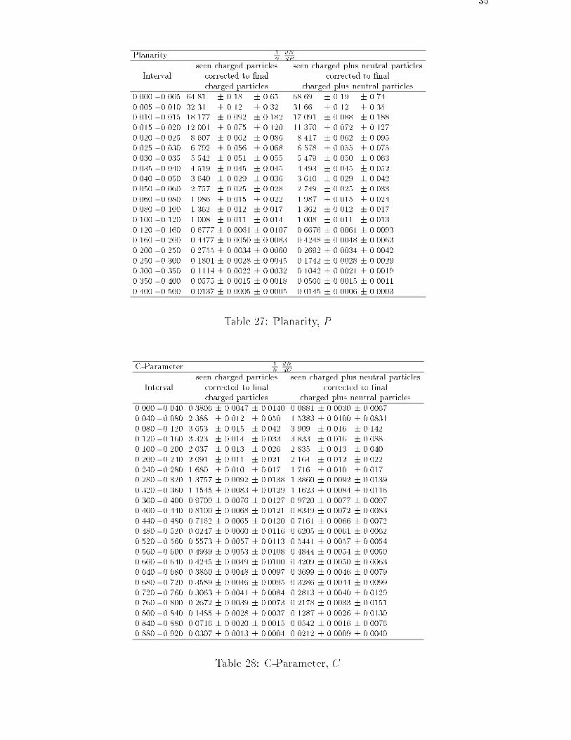
35

Planarity 1N

dNdP

seen charged particles seen charged plus neutral particlesInterval corrected to �nal corrected to �nal

charged particles charged plus neutral particles0.000 - 0.005 64.81 � 0.18 � 0.65 68.69 � 0.19 � 0.740.005 - 0.010 32.31 � 0.12 � 0.32 31.66 � 0.12 � 0.350.010 - 0.015 18.177 � 0.092 � 0.182 17.091 � 0.088 � 0.1880.015 - 0.020 12.001 � 0.075 � 0.120 11.370 � 0.072 � 0.1270.020 - 0.025 8.607 � 0.062 � 0.086 8.417 � 0.062 � 0.0950.025 - 0.030 6.792 � 0.056 � 0.068 6.578 � 0.055 � 0.0750.030 - 0.035 5.542 � 0.051 � 0.055 5.479 � 0.050 � 0.0630.035 - 0.040 4.519 � 0.045 � 0.045 4.493 � 0.045 � 0.0520.040 - 0.050 3.640 � 0.029 � 0.036 3.610 � 0.029 � 0.0420.050 - 0.060 2.757 � 0.025 � 0.028 2.749 � 0.025 � 0.0330.060 - 0.080 1.986 � 0.015 � 0.022 1.987 � 0.015 � 0.0240.080 - 0.100 1.362 � 0.012 � 0.017 1.362 � 0.012 � 0.0170.100 - 0.120 1.008 � 0.011 � 0.014 1.008 � 0.011 � 0.0130.120 - 0.160 0.6777 � 0.0061 � 0.0107 0.6676 � 0.0061 � 0.00930.160 - 0.200 0.4477 � 0.0050 � 0.0083 0.4248 � 0.0048 � 0.00630.200 - 0.250 0.2755 � 0.0034 � 0.0060 0.2692 � 0.0034 � 0.00420.250 - 0.300 0.1801 � 0.0028 � 0.0045 0.1742 � 0.0028 � 0.00290.300 - 0.350 0.1114 � 0.0022 � 0.0032 0.1042 � 0.0021 � 0.00190.350 - 0.400 0.0575 � 0.0015 � 0.0018 0.0566 � 0.0015 � 0.00110.400 - 0.500 0.0137 � 0.0005 � 0.0005 0.0145 � 0.0006 � 0.0003

Table 27: Planarity, P

C-Parameter 1N

dNdC

seen charged particles seen charged plus neutral particlesInterval corrected to �nal corrected to �nal

charged particles charged plus neutral particles

0.000 - 0.040 0.3806 � 0.0047 � 0.0140 0.0881 � 0.0030 � 0.00670.040 - 0.080 2.388 � 0.012 � 0.050 1.5383 � 0.0100 � 0.08310.080 - 0.120 3.653 � 0.015 � 0.042 3.909 � 0.016 � 0.1420.120 - 0.160 3.323 � 0.014 � 0.033 3.833 � 0.016 � 0.0880.160 - 0.200 2.637 � 0.013 � 0.026 2.835 � 0.013 � 0.0400.200 - 0.240 2.091 � 0.011 � 0.021 2.164 � 0.012 � 0.0220.240 - 0.280 1.680 � 0.010 � 0.017 1.716 � 0.010 � 0.0170.280 - 0.320 1.3757 � 0.0092 � 0.0138 1.3860 � 0.0092 � 0.01390.320 - 0.360 1.1545 � 0.0083 � 0.0129 1.1623 � 0.0084 � 0.01160.360 - 0.400 0.9709 � 0.0076 � 0.0127 0.9720 � 0.0077 � 0.00970.400 - 0.440 0.8100 � 0.0068 � 0.0121 0.8349 � 0.0072 � 0.00830.440 - 0.480 0.7162 � 0.0065 � 0.0120 0.7161 � 0.0066 � 0.00720.480 - 0.520 0.6247 � 0.0060 � 0.0116 0.6205 � 0.0061 � 0.00620.520 - 0.560 0.5573 � 0.0057 � 0.0113 0.5441 � 0.0057 � 0.00540.560 - 0.600 0.4939 � 0.0053 � 0.0108 0.4844 � 0.0054 � 0.00500.600 - 0.640 0.4245 � 0.0049 � 0.0100 0.4209 � 0.0050 � 0.00630.640 - 0.680 0.3860 � 0.0048 � 0.0097 0.3699 � 0.0046 � 0.00790.680 - 0.720 0.3589 � 0.0046 � 0.0095 0.3286 � 0.0044 � 0.00990.720 - 0.760 0.3063 � 0.0041 � 0.0084 0.2813 � 0.0040 � 0.01290.760 - 0.800 0.2672 � 0.0039 � 0.0073 0.2178 � 0.0033 � 0.01510.800 - 0.840 0.1485 � 0.0028 � 0.0037 0.1287 � 0.0026 � 0.01300.840 - 0.880 0.0716 � 0.0020 � 0.0015 0.0542 � 0.0016 � 0.00760.880 - 0.920 0.0307 � 0.0013 � 0.0004 0.0212 � 0.0009 � 0.0040

Table 28: C-Parameter, C

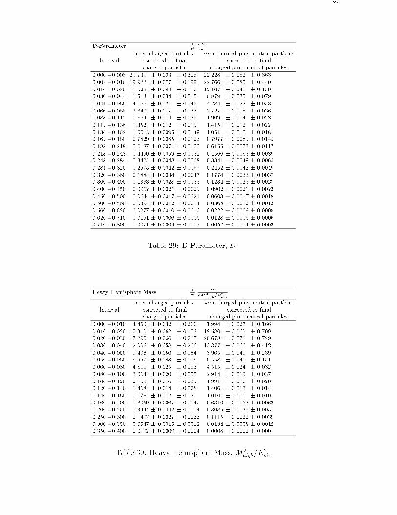
36

D-Parameter 1N

dNdD

seen charged particles seen charged plus neutral particlesInterval corrected to �nal corrected to �nal

charged particles charged plus neutral particles0.000 - 0.008 29.731 � 0.093 � 0.308 22.228 � 0.082 � 0.8680.008 - 0.016 19.922 � 0.077 � 0.199 22.766 � 0.085 � 0.4400.016 - 0.030 11.026 � 0.044 � 0.110 12.107 � 0.047 � 0.1500.030 - 0.044 6.513 � 0.034 � 0.065 6.879 � 0.035 � 0.0790.044 - 0.066 4.066 � 0.021 � 0.045 4.284 � 0.022 � 0.0530.066 - 0.088 2.640 � 0.017 � 0.033 2.727 � 0.018 � 0.0360.088 - 0.112 1.864 � 0.014 � 0.025 1.909 � 0.014 � 0.0280.112 - 0.136 1.352 � 0.012 � 0.019 1.415 � 0.012 � 0.0220.136 - 0.162 1.0013 � 0.0095 � 0.0149 1.051 � 0.010 � 0.0180.162 - 0.188 0.7829 � 0.0085 � 0.0123 0.7977 � 0.0089 � 0.01450.188 - 0.218 0.6187 � 0.0071 � 0.0103 0.6155 � 0.0073 � 0.01170.218 - 0.248 0.4490 � 0.0059 � 0.0081 0.4566 � 0.0063 � 0.00890.248 - 0.284 0.3425 � 0.0048 � 0.0068 0.3341 � 0.0049 � 0.00650.284 - 0.320 0.2575 � 0.0042 � 0.0057 0.2452 � 0.0042 � 0.00490.320 - 0.360 0.1884 � 0.0034 � 0.0047 0.1774 � 0.0033 � 0.00370.360 - 0.400 0.1363 � 0.0028 � 0.0038 0.1234 � 0.0028 � 0.00280.400 - 0.450 0.0962 � 0.0021 � 0.0029 0.0902 � 0.0021 � 0.00230.450 - 0.500 0.0644 � 0.0017 � 0.0021 0.0603 � 0.0017 � 0.00180.500 - 0.560 0.0394 � 0.0012 � 0.0014 0.0368 � 0.0012 � 0.00130.560 - 0.620 0.0277 � 0.0010 � 0.0010 0.0222 � 0.0009 � 0.00090.620 - 0.710 0.0151 � 0.0006 � 0.0006 0.0128 � 0.0006 � 0.00060.710 - 0.800 0.0071 � 0.0004 � 0.0003 0.0052 � 0.0004 � 0.0003

Table 29: D-Parameter, D

Heavy Hemisphere Mass 1N

dN

dM2high

=E2vis

seen charged particles seen charged plus neutral particlesInterval corrected to �nal corrected to �nal

charged particles charged plus neutral particles0.000 - 0.010 4.450 � 0.032 � 0.260 1.994 � 0.027 � 0.1660.010 - 0.020 17.310 � 0.062 � 0.173 18.580 � 0.065 � 0.7090.020 - 0.030 17.290 � 0.066 � 0.267 20.678 � 0.076 � 0.7290.030 - 0.040 12.996 � 0.058 � 0.206 13.377 � 0.060 � 0.4120.040 - 0.050 9.496 � 0.050 � 0.154 8.965 � 0.049 � 0.2390.050 - 0.060 6.957 � 0.043 � 0.116 6.558 � 0.041 � 0.1510.060 - 0.080 4.811 � 0.025 � 0.083 4.515 � 0.024 � 0.0820.080 - 0.100 3.064 � 0.020 � 0.055 2.914 � 0.019 � 0.0370.100 - 0.120 2.109 � 0.016 � 0.039 1.991 � 0.016 � 0.0200.120 - 0.140 1.468 � 0.014 � 0.028 1.406 � 0.013 � 0.0140.140 - 0.160 1.078 � 0.012 � 0.021 1.010 � 0.011 � 0.0100.160 - 0.200 0.6959 � 0.0067 � 0.0142 0.6319 � 0.0063 � 0.00630.200 - 0.250 0.3444 � 0.0042 � 0.0074 0.3085 � 0.0039 � 0.00510.250 - 0.300 0.1497 � 0.0027 � 0.0033 0.1115 � 0.0022 � 0.00390.300 - 0.350 0.0547 � 0.0015 � 0.0012 0.0184 � 0.0008 � 0.00120.350 - 0.400 0.0192 � 0.0009 � 0.0004 0.0008 � 0.0002 � 0.0001

Table 30: Heavy Hemisphere Mass, M2

high=E2

vis

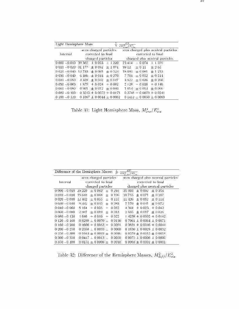
37

Light Hemisphere Mass 1N

dN

dM2low

=E2vis

seen charged particles seen charged plus neutral particlesInterval corrected to �nal corrected to �nal

charged particles charged plus neutral particles0.000 - 0.010 39.362 � 0.093 � 1.220 23.414 � 0.074 � 1.5950.010 - 0.020 31.177 � 0.092 � 1.074 39.12 � 0.11 � 2.650.020 - 0.030 13.733 � 0.065 � 0.523 18.080 � 0.081 � 1.2150.030 - 0.040 6.486 � 0.044 � 0.270 7.704 � 0.052 � 0.5140.040 - 0.050 3.358 � 0.032 � 0.147 3.922 � 0.036 � 0.2600.050 - 0.060 1.879 � 0.024 � 0.082 2.128 � 0.026 � 0.1400.060 - 0.080 0.901 � 0.012 � 0.040 1.013 � 0.013 � 0.0660.080 - 0.100 0.3212 � 0.0072 � 0.0175 0.3748 � 0.0079 � 0.02410.100 - 0.120 0.1087 � 0.0044 � 0.0082 0.1412 � 0.0050 � 0.0089

Table 31: Light Hemisphere Mass, M2

low=E2

vis

Di�erence of the Hemisphere Masses 1N

dN

dM2diff

=E2vis

seen charged particles seen charged plus neutral particlesInterval corrected to �nal corrected to �nal

charged particles charged plus neutral particles0.000 - 0.010 29.229 � 0.082 � 0.292 35.393 � 0.092 � 0.3540.010 - 0.020 19.648 � 0.068 � 0.196 20.745 � 0.071 � 0.2070.020 - 0.030 12.462 � 0.055 � 0.125 11.426 � 0.052 � 0.1140.030 - 0.040 8.332 � 0.045 � 0.083 7.170 � 0.041 � 0.0720.040 - 0.060 5.164 � 0.025 � 0.052 4.344 � 0.023 � 0.0430.060 - 0.080 2.987 � 0.019 � 0.034 2.605 � 0.017 � 0.0260.080 - 0.120 1.646 � 0.010 � 0.022 1.4238 � 0.0092 � 0.01420.120 - 0.160 0.8298 � 0.0070 � 0.0136 0.7061 � 0.0064 � 0.00710.160 - 0.200 0.4606 � 0.0053 � 0.0091 0.3831 � 0.0046 � 0.00440.200 - 0.250 0.2358 � 0.0033 � 0.0060 0.1836 � 0.0028 � 0.00320.250 - 0.300 0.1043 � 0.0022 � 0.0036 0.0579 � 0.0015 � 0.00180.300 - 0.350 0.0417 � 0.0013 � 0.0020 0.0075 � 0.0006 � 0.00060.350 - 0.400 0.0151 � 0.0008 � 0.0010 0.0003 � 0.0002 � 0.0001

Table 32: Di�erence of the Hemisphere Masses, M2

diff=E2

vis

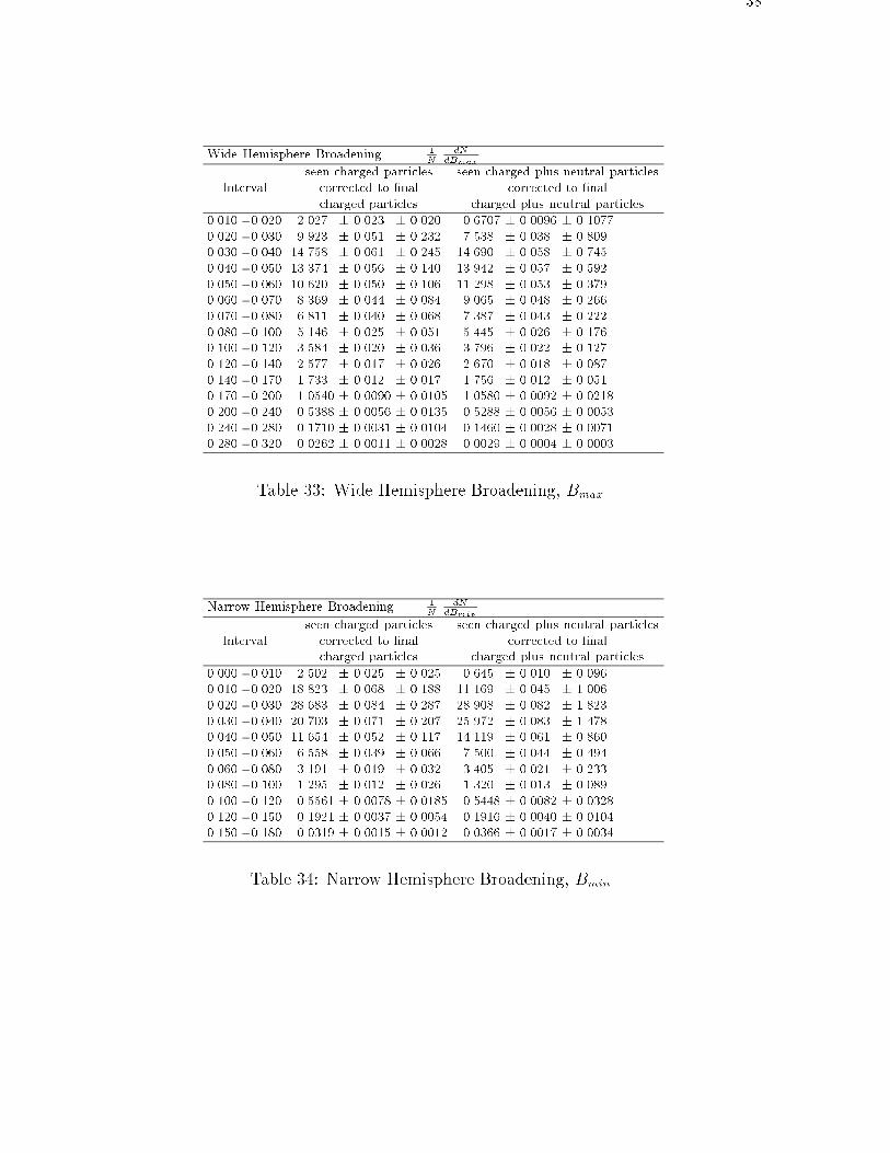
38

Wide Hemisphere Broadening 1N

dNdBmax

seen charged particles seen charged plus neutral particlesInterval corrected to �nal corrected to �nal

charged particles charged plus neutral particles0.010 - 0.020 2.027 � 0.023 � 0.020 0.6707 � 0.0096 � 0.10770.020 - 0.030 9.923 � 0.051 � 0.232 7.538 � 0.038 � 0.8090.030 - 0.040 14.758 � 0.061 � 0.245 14.690 � 0.058 � 0.7450.040 - 0.050 13.374 � 0.056 � 0.140 13.942 � 0.057 � 0.5920.050 - 0.060 10.620 � 0.050 � 0.106 11.298 � 0.053 � 0.3790.060 - 0.070 8.369 � 0.044 � 0.084 9.065 � 0.048 � 0.2660.070 - 0.080 6.811 � 0.040 � 0.068 7.387 � 0.043 � 0.2220.080 - 0.100 5.146 � 0.025 � 0.051 5.445 � 0.026 � 0.1760.100 - 0.120 3.584 � 0.020 � 0.036 3.796 � 0.022 � 0.1270.120 - 0.140 2.577 � 0.017 � 0.026 2.670 � 0.018 � 0.0870.140 - 0.170 1.733 � 0.012 � 0.017 1.756 � 0.012 � 0.0510.170 - 0.200 1.0540 � 0.0090 � 0.0105 1.0580 � 0.0092 � 0.02180.200 - 0.240 0.5388 � 0.0056 � 0.0135 0.5288 � 0.0056 � 0.00530.240 - 0.280 0.1710 � 0.0031 � 0.0104 0.1460 � 0.0028 � 0.00710.280 - 0.320 0.0262 � 0.0011 � 0.0028 0.0029 � 0.0004 � 0.0003

Table 33: Wide Hemisphere Broadening, Bmax

Narrow Hemisphere Broadening 1N

dNdBmin

seen charged particles seen charged plus neutral particlesInterval corrected to �nal corrected to �nal

charged particles charged plus neutral particles

0.000 - 0.010 2.502 � 0.025 � 0.025 0.645 � 0.010 � 0.0960.010 - 0.020 18.823 � 0.068 � 0.188 11.169 � 0.045 � 1.0060.020 - 0.030 28.683 � 0.084 � 0.287 28.908 � 0.082 � 1.8230.030 - 0.040 20.703 � 0.071 � 0.207 25.972 � 0.083 � 1.4780.040 - 0.050 11.654 � 0.052 � 0.117 14.119 � 0.061 � 0.8600.050 - 0.060 6.558 � 0.039 � 0.066 7.500 � 0.044 � 0.4940.060 - 0.080 3.191 � 0.019 � 0.032 3.405 � 0.021 � 0.2330.080 - 0.100 1.295 � 0.012 � 0.026 1.320 � 0.013 � 0.0890.100 - 0.120 0.5561 � 0.0078 � 0.0185 0.5448 � 0.0082 � 0.03280.120 - 0.150 0.1921 � 0.0037 � 0.0054 0.1916 � 0.0040 � 0.01040.150 - 0.180 0.0319 � 0.0015 � 0.0012 0.0366 � 0.0017 � 0.0034

Table 34: Narrow Hemisphere Broadening, Bmin

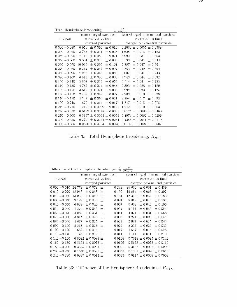
39

Total Hemisphere Broadening 1N

dNdBsum

seen charged particles seen charged plus neutral particlesInterval corrected to �nal corrected to �nal

charged particles charged plus neutral particles0.020 - 0.030 0.956 � 0.016 � 0.010 0.2030 � 0.0055 � 0.03830.030 - 0.040 3.765 � 0.031 � 0.038 1.628 � 0.015 � 0.1830.040 - 0.050 7.117 � 0.043 � 0.071 4.999 � 0.031 � 0.4630.050 - 0.060 9.301 � 0.048 � 0.093 8.190 � 0.041 � 0.6440.060 - 0.070 10.059 � 0.050 � 0.101 9.887 � 0.047 � 0.6610.070 - 0.080 9.212 � 0.047 � 0.092 9.883 � 0.049 � 0.5640.080 - 0.090 7.958 � 0.043 � 0.080 9.007 � 0.047 � 0.4430.090 - 0.100 6.815 � 0.040 � 0.068 7.746 � 0.044 � 0.3320.100 - 0.110 5.898 � 0.037 � 0.059 6.714 � 0.041 � 0.2550.110 - 0.130 4.785 � 0.024 � 0.048 5.393 � 0.026 � 0.1800.130 - 0.150 3.619 � 0.021 � 0.036 3.998 � 0.023 � 0.1250.150 - 0.170 2.737 � 0.018 � 0.027 2.980 � 0.019 � 0.0980.170 - 0.190 2.143 � 0.016 � 0.021 2.294 � 0.017 � 0.0850.190 - 0.210 1.670 � 0.014 � 0.017 1.747 � 0.015 � 0.0750.210 - 0.240 1.2151 � 0.0096 � 0.0122 1.242 � 0.010 � 0.0630.240 - 0.270 0.8189 � 0.0078 � 0.0082 0.8125 � 0.0080 � 0.04690.270 - 0.300 0.5167 � 0.0061 � 0.0065 0.4974 � 0.0062 � 0.02960.300 - 0.330 0.2701 � 0.0044 � 0.0054 0.2285 � 0.0041 � 0.01190.330 - 0.360 0.0856 � 0.0024 � 0.0028 0.0732 � 0.0024 � 0.0007

Table 35: Total Hemisphere Broadening, Bsum

Di�erence of the Hemisphere Broadenings 1N

dNdBdiff

seen charged particles seen charged plus neutral particlesInterval corrected to �nal corrected to �nal

charged particles charged plus neutral particles

0.000 - 0.010 24.778 � 0.078 � 0.248 26.630 � 0.081 � 0.4590.010 - 0.020 18.957 � 0.068 � 0.190 18.684 � 0.066 � 0.2920.020 - 0.030 13.050 � 0.056 � 0.131 12.343 � 0.054 � 0.1860.030 - 0.040 9.129 � 0.046 � 0.091 8.819 � 0.046 � 0.1340.040 - 0.050 6.689 � 0.040 � 0.067 6.688 � 0.040 � 0.1060.050 - 0.060 5.220 � 0.035 � 0.052 5.111 � 0.035 � 0.0840.060 - 0.070 4.087 � 0.031 � 0.041 4.071 � 0.031 � 0.0680.070 - 0.080 3.314 � 0.028 � 0.033 3.271 � 0.028 � 0.0540.080 - 0.090 2.677 � 0.025 � 0.027 2.681 � 0.025 � 0.0430.090 - 0.100 2.218 � 0.023 � 0.022 2.233 � 0.023 � 0.0350.100 - 0.120 1.662 � 0.014 � 0.017 1.647 � 0.014 � 0.0260.120 - 0.140 1.145 � 0.012 � 0.011 1.111 � 0.011 � 0.0190.140 - 0.160 0.8022 � 0.0098 � 0.0108 0.7618 � 0.0095 � 0.01440.160 - 0.180 0.5135 � 0.0078 � 0.0109 0.5138 � 0.0078 � 0.01190.180 - 0.200 0.3325 � 0.0063 � 0.0091 0.3167 � 0.0062 � 0.00980.200 - 0.240 0.1540 � 0.0029 � 0.0053 0.1265 � 0.0026 � 0.00560.240 - 0.280 0.0389 � 0.0014 � 0.0023 0.0117 � 0.0008 � 0.0008

Table 36: Di�erence of the Hemisphere Broadenings, Bdiff:

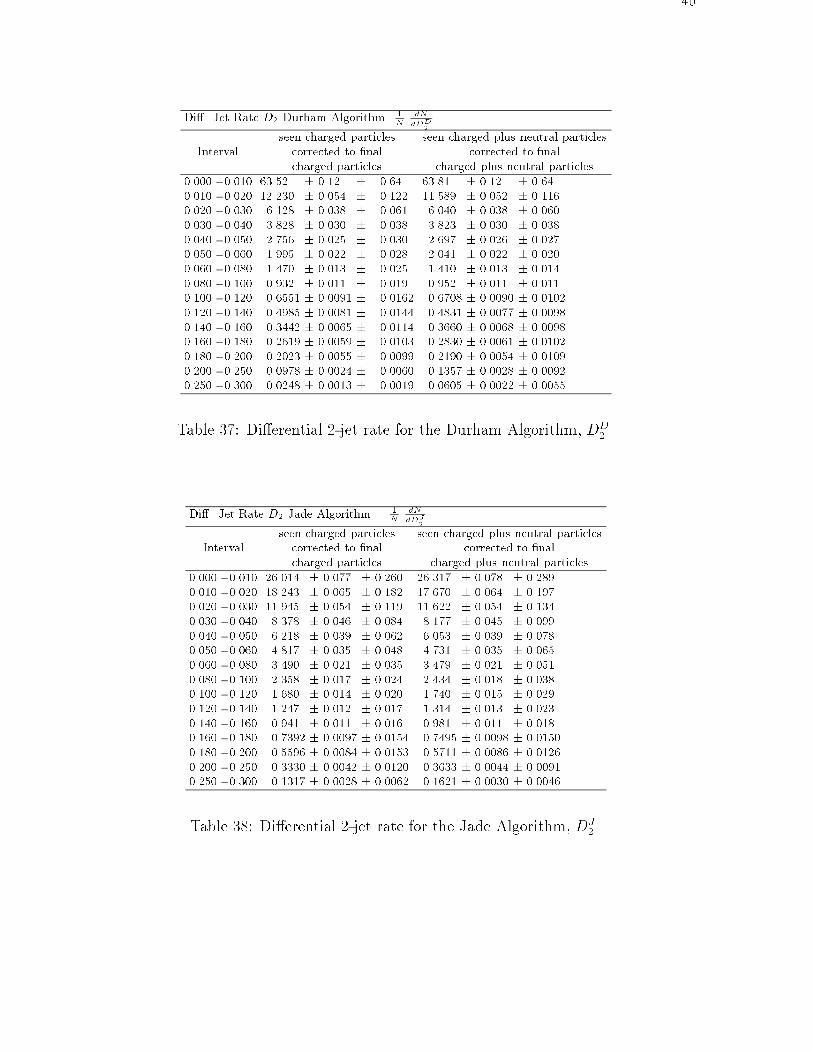
40

Di�. Jet Rate D2 Durham Algorithm 1N

dN

dDD2

seen charged particles seen charged plus neutral particlesInterval corrected to �nal corrected to �nal

charged particles charged plus neutral particles0.000 - 0.010 63.52 � 0.12 � 0.64 63.81 � 0.12 � 0.640.010 - 0.020 12.230 � 0.054 � 0.122 11.589 � 0.052 � 0.1160.020 - 0.030 6.128 � 0.038 � 0.061 6.040 � 0.038 � 0.0600.030 - 0.040 3.828 � 0.030 � 0.038 3.823 � 0.030 � 0.0380.040 - 0.050 2.756 � 0.025 � 0.030 2.697 � 0.026 � 0.0270.050 - 0.060 1.995 � 0.022 � 0.028 2.041 � 0.022 � 0.0200.060 - 0.080 1.470 � 0.013 � 0.025 1.410 � 0.013 � 0.0140.080 - 0.100 0.932 � 0.011 � 0.019 0.952 � 0.011 � 0.0110.100 - 0.120 0.6551 � 0.0091 � 0.0162 0.6708 � 0.0090 � 0.01020.120 - 0.140 0.4985 � 0.0081 � 0.0144 0.4831 � 0.0077 � 0.00980.140 - 0.160 0.3442 � 0.0065 � 0.0114 0.3660 � 0.0068 � 0.00980.160 - 0.180 0.2619 � 0.0059 � 0.0103 0.2830 � 0.0061 � 0.01020.180 - 0.200 0.2023 � 0.0055 � 0.0099 0.2190 � 0.0054 � 0.01090.200 - 0.250 0.0978 � 0.0024 � 0.0060 0.1357 � 0.0028 � 0.00920.250 - 0.300 0.0248 � 0.0013 � 0.0019 0.0605 � 0.0022 � 0.0055

Table 37: Di�erential 2-jet rate for the Durham Algorithm, DD2

Di�. Jet Rate D2 Jade Algorithm1N

dN

dDJ2

seen charged particles seen charged plus neutral particlesInterval corrected to �nal corrected to �nal

charged particles charged plus neutral particles0.000 - 0.010 26.014 � 0.077 � 0.260 26.317 � 0.078 � 0.2890.010 - 0.020 18.243 � 0.065 � 0.182 17.670 � 0.064 � 0.1970.020 - 0.030 11.945 � 0.054 � 0.119 11.622 � 0.054 � 0.1340.030 - 0.040 8.378 � 0.046 � 0.084 8.177 � 0.045 � 0.0990.040 - 0.050 6.218 � 0.039 � 0.062 6.053 � 0.039 � 0.0780.050 - 0.060 4.817 � 0.035 � 0.048 4.731 � 0.035 � 0.0650.060 - 0.080 3.490 � 0.021 � 0.035 3.479 � 0.021 � 0.0510.080 - 0.100 2.358 � 0.017 � 0.024 2.434 � 0.018 � 0.0380.100 - 0.120 1.680 � 0.014 � 0.020 1.740 � 0.015 � 0.0290.120 - 0.140 1.247 � 0.012 � 0.017 1.314 � 0.013 � 0.0230.140 - 0.160 0.941 � 0.011 � 0.016 0.981 � 0.011 � 0.0180.160 - 0.180 0.7392 � 0.0097 � 0.0154 0.7495 � 0.0098 � 0.01500.180 - 0.200 0.5596 � 0.0084 � 0.0153 0.5711 � 0.0086 � 0.01260.200 - 0.250 0.3330 � 0.0042 � 0.0120 0.3633 � 0.0044 � 0.00910.250 - 0.300 0.1317 � 0.0028 � 0.0062 0.1621 � 0.0030 � 0.0046

Table 38: Di�erential 2-jet rate for the Jade Algorithm, DJ2

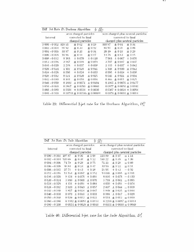
41

Di�. Jet Rate D3 Durham Algorithm 1N

dN

dDD3

seen charged particles seen charged plus neutral particlesInterval corrected to �nal corrected to �nal

charged particles charged plus neutral particles0.000 - 0.002 318.65 � 0.62 � 3.19 333.97 � 0.64 � 3.340.002 - 0.004 91.82 � 0.33 � 0.92 85.51 � 0.31 � 0.860.004 - 0.006 33.87 � 0.20 � 0.34 29.49 � 0.18 � 0.290.006 - 0.008 16.86 � 0.14 � 0.17 14.78 � 0.13 � 0.150.008 - 0.012 8.383 � 0.070 � 0.120 7.583 � 0.067 � 0.0760.012 - 0.016 3.967 � 0.048 � 0.079 3.707 � 0.047 � 0.0370.016 - 0.020 2.218 � 0.037 � 0.058 2.119 � 0.037 � 0.0420.020 - 0.024 1.302 � 0.028 � 0.041 1.348 � 0.030 � 0.0420.024 - 0.028 0.906 � 0.024 � 0.033 0.906 � 0.024 � 0.0380.028 - 0.032 0.621 � 0.020 � 0.025 0.646 � 0.021 � 0.0340.032 - 0.040 0.344 � 0.010 � 0.016 0.366 � 0.011 � 0.0250.040 - 0.050 0.1892 � 0.0071 � 0.0104 0.1965 � 0.0076 � 0.01770.050 - 0.060 0.0867 � 0.0050 � 0.0060 0.0877 � 0.0050 � 0.01000.060 - 0.080 0.0331 � 0.0024 � 0.0030 0.0367 � 0.0024 � 0.00540.080 - 0.100 0.00742 � 0.00136 � 0.00088 0.0073 � 0.0010 � 0.0014

Table 39: Di�erential 3-jet rate for the Durham Algorithm, DD3

Di�. Jet Rate D3 Jade Algorithm 1N

dN

dDJ3

seen charged particles seen charged plus neutral particlesInterval corrected to �nal corrected to �nal

charged particles charged plus neutral particles0.000 - 0.002 107.87 � 0.36 � 1.08 113.89 � 0.37 � 1.140.002 - 0.004 121.68 � 0.38 � 1.22 130.22 � 0.39 � 1.300.004 - 0.006 74.79 � 0.29 � 0.75 71.16 � 0.28 � 0.800.006 - 0.008 46.84 � 0.23 � 0.47 43.53 � 0.22 � 0.510.008 - 0.012 27.71 � 0.13 � 0.28 25.56 � 0.12 � 0.320.012 - 0.016 15.164 � 0.097 � 0.152 14.035 � 0.095 � 0.1910.016 - 0.020 9.124 � 0.075 � 0.091 8.816 � 0.075 � 0.1330.020 - 0.024 5.939 � 0.060 � 0.070 5.733 � 0.061 � 0.0950.024 - 0.028 4.101 � 0.051 � 0.064 4.009 � 0.051 � 0.0740.028 - 0.032 2.920 � 0.043 � 0.057 2.897 � 0.044 � 0.0590.032 - 0.040 1.857 � 0.024 � 0.047 1.849 � 0.025 � 0.0440.040 - 0.050 0.970 � 0.016 � 0.033 0.988 � 0.017 � 0.0290.050 - 0.060 0.509 � 0.012 � 0.022 0.513 � 0.012 � 0.0190.060 - 0.080 0.1952 � 0.0051 � 0.0113 0.2203 � 0.0057 � 0.01140.080 - 0.100 0.0554 � 0.0029 � 0.0043 0.0654 � 0.0033 � 0.0049

Table 40: Di�erential 3-jet rate for the Jade Algorithm, DJ3

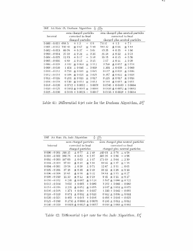
42

Di�. Jet Rate D4 Durham Algorithm 1N

dN

dDD4

seen charged particles seen charged plus neutral particlesInterval corrected to �nal corrected to �nal

charged particles charged plus neutral particles

0.000 - 0.001 688.3 � 1.3 � 6.9 711.0 � 1.3 � 7.10.001 - 0.002 190.40 � 0.67 � 1.90 184.32 � 0.66 � 1.840.002 - 0.003 60.98 � 0.37 � 0.61 53.35 � 0.35 � 1.060.003 - 0.004 25.69 � 0.24 � 0.26 21.18 � 0.22 � 0.530.004 - 0.005 12.63 � 0.17 � 0.18 10.15 � 0.15 � 0.300.005 - 0.006 6.89 � 0.13 � 0.15 5.67 � 0.11 � 0.200.006 - 0.008 3.442 � 0.063 � 0.112 2.768 � 0.057 � 0.1140.008 - 0.010 1.454 � 0.040 � 0.068 1.203 � 0.039 � 0.0600.010 - 0.012 0.750 � 0.031 � 0.045 0.617 � 0.028 � 0.0360.012 - 0.014 0.348 � 0.020 � 0.025 0.357 � 0.022 � 0.0240.014 - 0.016 0.204 � 0.016 � 0.017 0.215 � 0.017 � 0.0160.016 - 0.018 0.130 � 0.013 � 0.013 0.144 � 0.015 � 0.0110.018 - 0.020 0.0712 � 0.0092 � 0.0078 0.0745 � 0.0103 � 0.00640.020 - 0.025 0.0342 � 0.0041 � 0.0044 0.0434 � 0.0052 � 0.00420.025 - 0.030 0.0110 � 0.0023 � 0.0017 0.0133 � 0.0028 � 0.0014

Table 41: Di�erential 4-jet rate for the Durham Algorithm, DD4

Di�. Jet Rate D4 Jade Algorithm 1N

dN

dDJ4

seen charged particles seen charged plus neutral particlesInterval corrected to �nal corrected to �nal

charged particles charged plus neutral particles

0.000 - 0.001 248.15 � 0.77 � 2.48 240.63 � 0.78 � 4.580.001 - 0.002 286.76 � 0.82 � 2.87 309.26 � 0.86 � 4.960.002 - 0.003 167.03 � 0.63 � 1.67 171.69 � 0.64 � 2.390.003 - 0.004 97.00 � 0.48 � 1.04 92.65 � 0.47 � 1.180.004 - 0.005 59.58 � 0.38 � 0.71 52.87 � 0.35 � 0.650.005 - 0.006 37.48 � 0.30 � 0.49 33.41 � 0.28 � 0.430.006 - 0.008 21.61 � 0.16 � 0.32 18.83 � 0.15 � 0.270.008 - 0.010 11.10 � 0.12 � 0.19 9.45 � 0.11 � 0.170.010 - 0.012 6.235 � 0.087 � 0.124 5.567 � 0.086 � 0.1220.012 - 0.014 3.602 � 0.065 � 0.080 3.262 � 0.066 � 0.0890.014 - 0.016 2.205 � 0.052 � 0.055 2.047 � 0.052 � 0.0700.016 - 0.018 1.373 � 0.041 � 0.037 1.330 � 0.042 � 0.0550.018 - 0.020 0.874 � 0.032 � 0.026 0.912 � 0.036 � 0.0440.020 - 0.025 0.460 � 0.015 � 0.016 0.456 � 0.016 � 0.0250.025 - 0.030 0.1735 � 0.0096 � 0.0070 0.195 � 0.011 � 0.0120.030 - 0.050 0.0303 � 0.0021 � 0.0017 0.034 � 0.003 � 0.002

Table 42: Di�erential 4-jet rate for the Jade Algorithm, DJ4

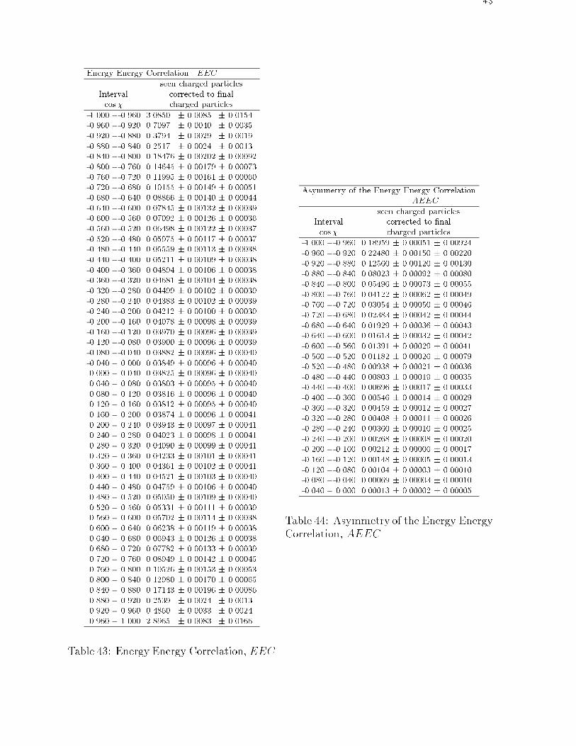
43

Energy Energy Correlation EEC

seen charged particlesInterval corrected to �nalcos� charged particles

-1.000 - -0.960 3.0850 � 0.0085 � 0.0154-0.960 - -0.920 0.7097 � 0.0040 � 0.0035-0.920 - -0.880 0.3794 � 0.0029 � 0.0019-0.880 - -0.840 0.2517 � 0.0024 � 0.0013-0.840 - -0.800 0.18476 � 0.00202 � 0.00092-0.800 - -0.760 0.14645 � 0.00179 � 0.00073-0.760 - -0.720 0.11995 � 0.00161 � 0.00060-0.720 - -0.680 0.10155 � 0.00149 � 0.00051-0.680 - -0.640 0.08866 � 0.00140 � 0.00044-0.640 - -0.600 0.07845 � 0.00132 � 0.00039-0.600 - -0.560 0.07092 � 0.00126 � 0.00036-0.560 - -0.520 0.06498 � 0.00122 � 0.00037-0.520 - -0.480 0.05975 � 0.00117 � 0.00037-0.480 - -0.440 0.05559 � 0.00113 � 0.00038-0.440 - -0.400 0.05211 � 0.00109 � 0.00038-0.400 - -0.360 0.04894 � 0.00106 � 0.00038-0.360 - -0.320 0.04681 � 0.00104 � 0.00038-0.320 - -0.280 0.04499 � 0.00102 � 0.00039-0.280 - -0.240 0.04383 � 0.00102 � 0.00039-0.240 - -0.200 0.04212 � 0.00100 � 0.00039-0.200 - -0.160 0.04078 � 0.00098 � 0.00039-0.160 - -0.120 0.03970 � 0.00096 � 0.00039-0.120 - -0.080 0.03900 � 0.00096 � 0.00039-0.080 - -0.040 0.03882 � 0.00096 � 0.00040-0.040 - 0.000 0.03849 � 0.00096 � 0.000400.000 - 0.040 0.03825 � 0.00096 � 0.000400.040 - 0.080 0.03803 � 0.00095 � 0.000400.080 - 0.120 0.03816 � 0.00096 � 0.000400.120 - 0.160 0.03812 � 0.00095 � 0.000400.160 - 0.200 0.03874 � 0.00096 � 0.000410.200 - 0.240 0.03943 � 0.00097 � 0.000410.240 - 0.280 0.04023 � 0.00098 � 0.000410.280 - 0.320 0.04090 � 0.00099 � 0.000410.320 - 0.360 0.04233 � 0.00101 � 0.000410.360 - 0.400 0.04361 � 0.00102 � 0.000410.400 - 0.440 0.04521 � 0.00103 � 0.000400.440 - 0.480 0.04759 � 0.00106 � 0.000400.480 - 0.520 0.05050 � 0.00109 � 0.000400.520 - 0.560 0.05331 � 0.00111 � 0.000390.560 - 0.600 0.05702 � 0.00114 � 0.000380.600 - 0.640 0.06238 � 0.00119 � 0.000380.640 - 0.680 0.06943 � 0.00126 � 0.000380.680 - 0.720 0.07782 � 0.00133 � 0.000390.720 - 0.760 0.08949 � 0.00142 � 0.000450.760 - 0.800 0.10526 � 0.00153 � 0.000530.800 - 0.840 0.12980 � 0.00170 � 0.000650.840 - 0.880 0.17143 � 0.00196 � 0.000860.880 - 0.920 0.2539 � 0.0024 � 0.00130.920 - 0.960 0.4860 � 0.0033 � 0.00240.960 - 1.000 2.8965 � 0.0083 � 0.0166

Table 43: Energy Energy Correlation, EEC

Asymmetry of the Energy Energy CorrelationAEEC

seen charged particlesInterval corrected to �nalcos� charged particles

-1.000 - -0.960 0.18959 � 0.00051 � 0.00924-0.960 - -0.920 0.22480 � 0.00150 � 0.00220-0.920 - -0.880 0.12560 � 0.00120 � 0.00130-0.880 - -0.840 0.08023 � 0.00092 � 0.00080-0.840 - -0.800 0.05496 � 0.00073 � 0.00055-0.800 - -0.760 0.04122 � 0.00062 � 0.00049-0.760 - -0.720 0.03054 � 0.00050 � 0.00046-0.720 - -0.680 0.02383 � 0.00042 � 0.00044-0.680 - -0.640 0.01929 � 0.00036 � 0.00043-0.640 - -0.600 0.01613 � 0.00032 � 0.00042-0.600 - -0.560 0.01391 � 0.00029 � 0.00041-0.560 - -0.520 0.01182 � 0.00026 � 0.00079-0.520 - -0.480 0.00938 � 0.00021 � 0.00036-0.480 - -0.440 0.00803 � 0.00019 � 0.00035-0.440 - -0.400 0.00696 � 0.00017 � 0.00033-0.400 - -0.360 0.00546 � 0.00014 � 0.00029-0.360 - -0.320 0.00459 � 0.00012 � 0.00027-0.320 - -0.280 0.00408 � 0.00011 � 0.00026-0.280 - -0.240 0.00360 � 0.00010 � 0.00025-0.240 - -0.200 0.00268 � 0.00008 � 0.00020-0.200 - -0.160 0.00212 � 0.00006 � 0.00017-0.160 - -0.120 0.00148 � 0.00005 � 0.00013-0.120 - -0.080 0.00104 � 0.00003 � 0.00010-0.080 - -0.040 0.00069 � 0.00003 � 0.00010-0.040 - 0.000 0.00013 � 0.00002 � 0.00005

Table 44: Asymmetry of the Energy EnergyCorrelation, AEEC

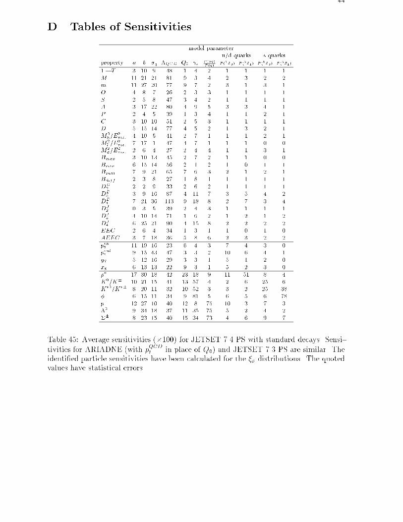
44

D Tables of Sensitivities

model parameteru/d quarks s quarks

property a b �q �QCD Q0 s P(qq)

P (q)P(1S0) P (3S1) P (1S0) P(3S1)

1� T 3 10 9 48 1 4 2 1 1 1 1M 11 21 21 81 9 3 4 2 3 2 2m 11 27 20 77 9 7 2 3 1 3 1O 4 8 7 26 2 3 3 1 1 1 1S 2 5 8 47 3 4 2 1 1 1 1A 3 17 22 80 4 9 5 3 3 4 1P 2 4 5 39 1 3 4 1 1 2 1C 3 10 10 51 2 5 3 1 1 1 1D 5 15 14 77 4 5 2 1 3 2 1M2

h=E2vis: 4 10 5 41 2 7 1 1 1 2 1

M2l =E

2vis: 7 17 1 47 4 7 1 1 1 0 0

M2d =E

2vis: 2 6 4 27 2 4 4 1 1 3 1

Bmax 3 10 13 45 2 7 2 1 1 0 0Bmin 6 15 14 56 2 1 2 1 0 1 1Bsum 7 9 21 65 7 6 3 2 1 2 1Bdiff: 2 3 8 27 1 8 1 1 1 1 1DD

2 2 2 9 33 2 6 2 1 1 1 1DD

3 3 9 16 87 4 11 7 3 5 4 2DD

4 7 21 36 113 9 18 8 2 7 3 4DJ

2 0 3 5 39 2 4 3 1 1 1 1DJ

3 4 10 14 71 1 6 2 1 2 1 2DJ

4 6 25 21 90 4 15 8 2 2 2 2EEC 2 6 4 34 1 3 1 1 0 1 0AEEC 3 7 18 36 5 8 6 2 3 2 2

pint 11 19 16 23 6 4 3 7 4 3 0poutt 9 15 43 47 3 3 2 10 6 4 1yT 5 12 16 29 3 3 1 5 1 2 0xp 6 13 13 22 9 3 1 5 2 3 0�� 17 30 18 42 23 18 9 11 51 8 4K0=K� 10 21 15 41 13 57 4 2 6 25 6K�0=K�� 8 20 11 32 10 52 3 3 2 25 38� 6 15 11 34 9 81 5 6 5 6 78p 12 27 10 40 12 8 75 10 3 7 3�0 9 34 18 37 11 35 75 5 2 4 2�� 8 23 15 40 15 34 73 4 6 9 7

Table 45: Average sensitivities (�100) for JETSET 7.4 PS with standard decays. Sensi-

tivities for ARIADNE (with pQCDt in place of Q0) and JETSET 7.3 PS are similar. The

identi�ed particle sensitivities have been calculated for the �p distributions. The quotedvalues have statistical errors.

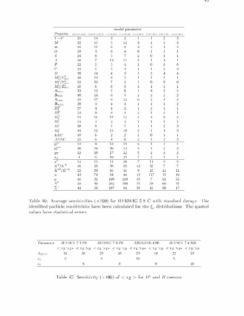
45

model parameterProperty QCDLAM RMASS(13) CLMAX CLPOW CLSMR PWT (3) PWT (7) DECWT

1� T 25 14 3 2 1 1 2 3M 32 15 5 12 3 1 2 3m 34 11 8 8 3 2 4 4O 19 3 6 4 0 1 1 1S 24 8 5 7 2 0 1 1A 50 7 13 11 4 1 3 1P 22 5 5 4 1 0 0 0C 22 5 5 4 1 1 2 3D 30 14 4 3 1 2 4 4M2

h=E2vis: 20 13 8 5 1 1 1 1

M2l =E

2vis: 22 22 7 2 1 0 0 0

M2d=E

2vis: 18 6 8 6 1 1 1 1

Bmax 33 12 7 6 1 4 2 5Bmin 40 14 6 5 2 2 2 2Bsum 29 17 6 22 6 2 4 3Bdiff: 20 3 4 3 1 1 1 2DD

2 27 4 4 2 1 2 1 1DD

3 53 9 8 4 2 1 2 1DD

4 74 11 17 12 4 4 8 2DJ

2 14 4 2 2 1 1 1 1DJ

3 38 9 7 7 1 1 2 3DJ

4 44 12 15 10 2 1 4 3EEC 18 6 2 2 1 0 1 1AEEC 25 6 8 6 2 1 2 3

pint 14 9 13 19 6 1 2 1poutt 30 10 30 13 4 1 2 3yT 12 10 17 22 5 2 2 2xp 4 6 10 25 7 2 1 1�� 12 15 14 36 7 14 9 9K0=K� 16 28 39 55 12 32 7 7K�0=K�� 22 39 16 41 9 45 12 11� 43 74 34 44 13 117 15 10p 16 21 199 119 15 7 61 55�0 29 40 262 100 15 58 60 41�� 44 58 187 64 35 42 60 17

Table 46: Average sensitivities (�100) for HERWIG 5.8 C with standard decays. Theidenti�ed particle sensitivities have been calculated for the �p distributions. The quotedvalues have statistical errors.

Parameter JETSET 7.3 PS JETSET 7.4 PS ARIADNE 4.06 JETSET 7.4 ME

< xE >D� < xE >B < xE >D� < xE >B < xE >D� < xE >B < xE >D� < xE >B

�QCD 32 30 29 26 23 18 22 23

�c 9 9 10 9

�b 8 8 9 10

Table 47: Sensitivity (�100) of < xE > for D� and B mesons

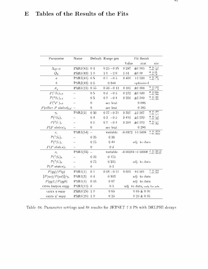
46

E Tables of the Results of the Fits

Parameter Name Default Range gen. Fit Result

Value stat. sys.

�QCD PARJ(81) 0.4 0.25 - 0.35 0.297 �0.005 +

�

0:0120:007

Q0 PARJ(82) 1.0 1.0 - 2.0 1.34 �0.08 +

�

0:150:09

a PARJ(41) 0.5 0.1 - 0.5 0.409 �0.020 +

�

0:0090:013

b PARJ(42) 0.9 0.844 optimized

�q PARJ(21) 0.35 0.36 - 0.44 0.401 �0.006 +

�

0:0030:013

P (1S0)ud - 0.5 0.3 - 0.5 0.272 �0.030 +

�

0:1080:008

P (3S1)ud - 0.5 0.2 - 0.4 0.306 �0.049 +

�

0:0060:031

P (1P1)ud - 0. see text 0.094

P (other P states)ud - 0. see text 0.305

s PARJ(2) 0.30 0.27 - 0.31 0.307 �0.007 +

�

0:0020:017

P (1S0)s - 0.4 0.3 - 0.5 0.416 �0.029 +

�

0:0150:003

P (3S1)s - 0.6 0.2 - 0.4 0.304 �0.023 +

�

0:0170:002

P (P states)s - 0. see text 0.280

�c PARJ(54) - variable -0.0372 �0.0008 +

�

0:00200:0012

P (1S0)c - 0.25 0.26

P (3S1)c - 0.75 0.44 adj. to data

P (P states)c - 0. 0.3

�b PARJ(55) - variable -0.00284�0.00006 +

�

0:000130:00009

P (1S0)b - 0.25 0.175

P (3S1)b - 0.75 0.525 adj. to data

P (P states)b - 0. 0.3

P (qq)=P (q) PARJ(1) 0.1 0.08 - 0.11 0.095 �0.001 +

�

0:0040:002

[P (us)=P (ud)]= s PARJ(3) 0.4 0.593 adj. to data

P (qq1)=P (qq0) PARJ(4) 0.05 0.07 adj. to data

extra baryon supp. PARJ(19) 0. 0.5 adj. to data, only for uds

extra � supp. PARJ(25) 1.0 0.65 0.65 � 0.06

extra �0 supp. PARJ(26) 1.0 0.23 0.23 � 0.05

Table 48: Parameter settings and �t results for JETSET 7.3 PS with DELPHI decays

47

Parameter Name Default Range gen. Fit Result

Value stat. sys.

�QCD PARJ(81) 0.29 0.25 - 0.35 0.297 �0.004 +

�

0:0070:008

Q0 PARJ(82) 1.0 1.0 - 2.0 1.56 �0.11 +

�

0:210:15

a PARJ(41) 0.3 0.1 - 0.5 0.417 �0.022 +

�

0:0110:015

b PARJ(42) 0.58 0.850 optimized

�q PARJ(21) 0.36 0.36 - 0.44 0.408 �0.005 +

�

0:0040:004

P (1S0)ud - 0.5 0.3 - 0.5 0.297 �0.021 +

�

0:1020:011

P (3S1)ud - 0.5 0.2 - 0.4 0.289 �0.038 +

�

0:0040:026

P (1P1)ud - 0. see text 0.096

P (other P states)ud - 0. see text 0.318

s PARJ(2) 0.30 0.27 - 0.31 0.308 �0.007 +

�

0:0040:036

P (1S0)s - 0.4 0.3 - 0.5 0.410 �0.038 +

�

0:0260:013

P (3S1)s - 0.6 0.2 - 0.4 0.297 �0.021 +

�

0:0200:004

P (P states)s - 0. see text 0.293

�c PARJ(54) - variable -0.0372 �0.0007 +

�

0:00110:0012

P (1S0)c - 0.25 0.26

P (3S1)c - 0.75 0.44 adj. to data

P (P states)c - 0. 0.3

�b PARJ(55) - variable -0.00284�0.00005 +

�

0:000120:00010

P (1S0)b - 0.25 0.175

P (3S1)b - 0.75 0.525 adj. to data

P (P states)b - 0. 0.3

P (qq)=P (q) PARJ(1) 0.1 0.08 - 0.11 0.099 �0.001 +

�

0:0050:002

[P (us)=P (ud)]= s PARJ(3) 0.4 0.593 adj. to data

P (qq1)=P (qq0) PARJ(4) 0.05 0.07 adj. to data

extra baryon supp. PARJ(19) 0. 0.5 adj. to data, only for uds

extra � supp. PARJ(25) 1.0 0.65 0.65 � 0.06

extra �0 supp. PARJ(26) 1.0 0.23 0.23 � 0.05

Table 49: Parameter settings and �t results for JETSET 7.4 PS with default decays

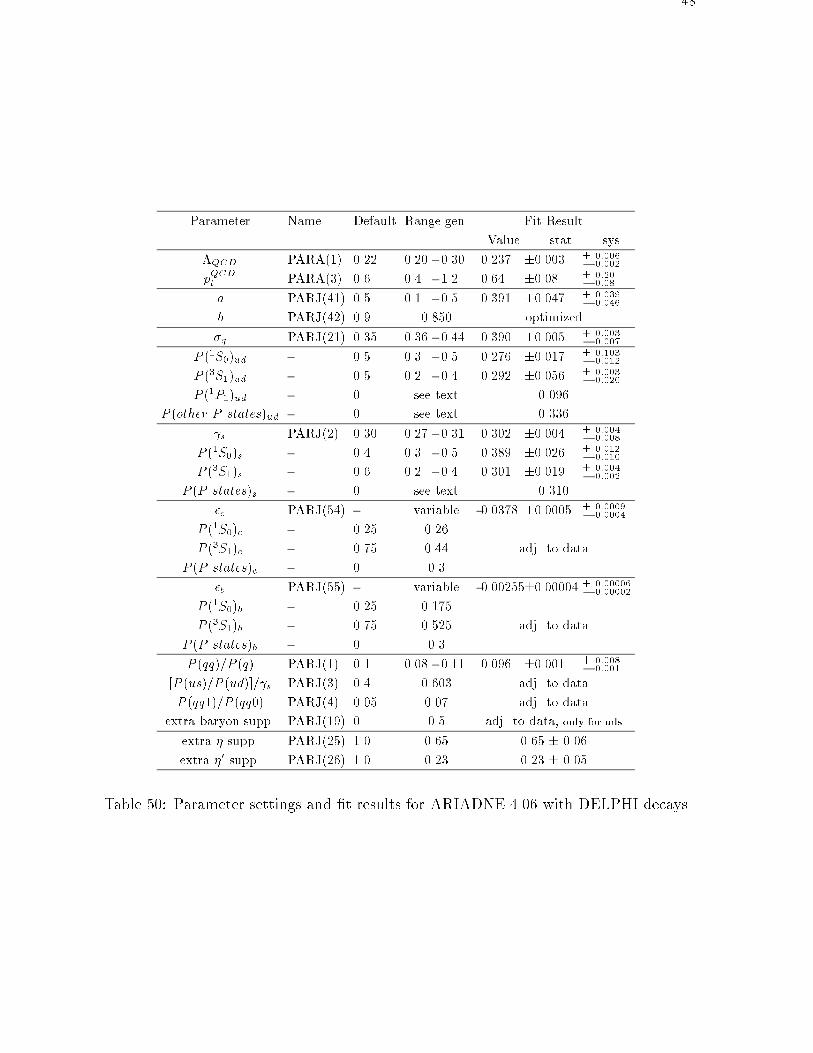
48

Parameter Name Default Range gen. Fit Result

Value stat. sys.

�QCD PARA(1) 0.22 0.20 - 0.30 0.237 �0.003 +

�

0:0060:002

pQCDt PARA(3) 0.6 0.4 - 1.2 0.64 �0.08 +

�

0:200:08

a PARJ(41) 0.5 0.1 - 0.5 0.391 �0.047 +

�

0:0390:046

b PARJ(42) 0.9 0.850 optimized

�q PARJ(21) 0.35 0.36 - 0.44 0.390 �0.005 +

�

0:0030:007

P (1S0)ud - 0.5 0.3 - 0.5 0.276 �0.017 +

�

0:1030:012

P (3S1)ud - 0.5 0.2 - 0.4 0.292 �0.056 +

�

0:0030:020

P (1P1)ud - 0. see text 0.096

P (other P states)ud - 0. see text 0.336

s PARJ(2) 0.30 0.27 - 0.31 0.302 �0.004 +

�

0:0040:008

P (1S0)s - 0.4 0.3 - 0.5 0.389 �0.026 +

�

0:0120:010

P (3S1)s - 0.6 0.2 - 0.4 0.301 �0.019 +

�

0:0040:002

P (P states)s - 0. see text 0.310

�c PARJ(54) - variable -0.0378 �0.0005 +

�

0:00090:0004

P (1S0)c - 0.25 0.26

P (3S1)c - 0.75 0.44 adj. to data

P (P states)c - 0. 0.3

�b PARJ(55) - variable -0.00255�0.00004 +

�

0:000060:00002

P (1S0)b - 0.25 0.175

P (3S1)b - 0.75 0.525 adj. to data

P (P states)b - 0. 0.3

P (qq)=P (q) PARJ(1) 0.1 0.08 - 0.11 0.096 �0.001 +

�

0:0080:001

[P (us)=P (ud)]= s PARJ(3) 0.4 0.603 adj. to data

P (qq1)=P (qq0) PARJ(4) 0.05 0.07 adj. to data

extra baryon supp. PARJ(19) 0. 0.5 adj. to data, only for uds

extra � supp. PARJ(25) 1.0 0.65 0.65 � 0.06

extra �0 supp. PARJ(26) 1.0 0.23 0.23 � 0.05

Table 50: Parameter settings and �t results for ARIADNE 4.06 with DELPHI decays

49

Parameter name Default Range gen. Fit Result

Value stat. sys.

�QCD PARA(1) 0.22 0.20 - 0.30 0.237 �0.004 +

�

0:0050:004

pQCDt PARA(3) 0.6 0.4 - 1.2 0.68 �0.06 +

�

0:110:11

a PARJ(41) 0.5 0.1 - 0.5 0.388 �0.030 +

�

0:0360:112

b PARJ(42) 0.9 0.850 optimized

�q PARJ(21) 0.35 0.36 - 0.44 0.387 �0.008 +

�

0:0120:016

P (1S0)ud - 0.5 0.3 - 0.5 0.326 �0.017 +

�

0:0580:023

P (3S1)ud - 0.5 0.2 - 0.4 0.263 �0.039 +

�

0:0150:010

P (1P1)ud - 0. see text 0.096

P (other P states)ud - 0. see text 0.411

s PARJ(2) 0.30 0.27 - 0.31 0.282 �0.005 +

�

0:0150:004

P (1S0)s - 0.4 0.3 - 0.5 0.395 �0.023 +

�

0:0080:040

P (3S1)s - 0.6 0.2 - 0.4 0.325 �0.015 +

�

0:0050:033

P (P states)s - 0. see text 0.280

�c PARJ(54) - variable -0.0378 �0.0005 +

�

0:00090:0004

P (1S0)c - 0.25 0.26

P (3S1)c - 0.75 0.44 adj. to data

P (P states)c - 0. 0.3

�b PARJ(55) - variable -0.00255�0.00004 +

�

0:000060:00002

P (1S0)b - 0.25 0.175

P (3S1)b - 0.75 0.525 adj. to data

P (P states)b - 0. 0.3

P (qq)=P (q) PARJ(1) 0.1 0.08 - 0.11 0.101 �0.001 +

�

0:0060:001

[P (us)=P (ud)]= s PARJ(3) 0.4 0.645 adj. to data

P (qq1)=P (qq0) PARJ(4) 0.05 0.07 adj. to data

extra baryon supp. PARJ(19) 0. 0.5 adj. to data, only for uds

extra � supp. PARJ(25) 1.0 0.65 0.65 � 0.06

extra �0 supp. PARJ(26) 1.0 0.23 0.23 � 0.05

Table 51: Parameter settings and �t results for ARIADNE 4.06 with default decays

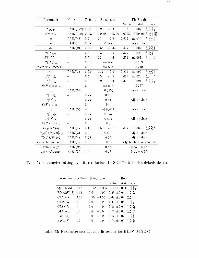
50

Parameter Name Default Range gen. Fit Result

Value stat. sys.

�QCD PARJ(122) 0.22 0.20 - 0.30 0.163 �0.002 +

�

0:0010:003

Scale � PARJ(129) 0.002 0.0005 - 0.0025 0.00250�0.00006 +

�

0:000130:00018

a PARJ(41) 0.3 0.1 - 0.5 0.903 �0.014 +

�

0:0380:014

b PARJ(42) 0.58 0.525 optimized

�q PARJ(21) 0.36 0.36 - 0.44 0.477 �0.004 +

�

0:0050:006

P (1S0)ud - 0.5 0.3 - 0.5 0.327 �0.023 +

�

0:0510:021

P (3S1)ud - 0.5 0.2 - 0.4 0.274 �0.061 +

�

0:0120:013

P (1P1)ud - 0. see text 0.089

P (other P states)ud - 0. see text 0.310

s PARJ(2) 0.30 0.27 - 0.31 0.277 �0.006 +

�

0:0080:004

P (1S0)s - 0.4 0.3 - 0.5 0.413 �0.028 +

�

0:0160:011

P (3S1)s - 0.6 0.2 - 0.4 0.330 �0.021 +

�

0:0110:008

P (P states)s - 0. see text 0.257

�c PARJ(54) - -0.0950 optimized

P (1S0)c - 0.25 0.26

P (3S1)c - 0.75 0.44 adj. to data

P (P states)c - 0. 0.3

�b PARJ(55) - -0.00427 optimized

P (1S0)b - 0.25 0.175

P (3S1)b - 0.75 0.525 adj. to data

P (P states)b - 0. 0.3

P (qq)=P (q) PARJ(1) 0.1 0.08 - 0.11 0.087 �0.002 +

�

0:0080:002

[P (us)=P (ud)]= s PARJ(3) 0.4 0.657 adj. to data

P (qq1)=P (qq0) PARJ(4) 0.05 0.07 adj. to data

extra baryon supp. PARJ(19) 0. 0.5 adj. to data, only for uds

extra � supp. PARJ(25) 1.0 0.65 0.65 � 0.06

extra �0 supp. PARJ(26) 1.0 0.23 0.23 � 0.05

Table 52: Parameter settings and �t results for JETSET 7.4 ME with default decays

Parameter Default Range gen. Fit Result

Value stat. sys.

QCDLAM 0.18 0.155 - 0.205 0.163�0.001 +

�

0:0040:005

RMASS(13) 0.75 0.64 - 0.96 0.65 �0.01 +

�

0:020:01

CLMAX 3.35 2.35 - 4.35 3.48 �0.04 +

�

0:200:13

CLPOW 2.0 1.0 - 2.0 1.49 �0.04 +

�

0:160:08

CLSMR 0. 0.0 - 1.0 0.36 �0.04 +

�

0:060:01

DECWT 1.0 0.0 - 1.0 0.77 �0.08 +

�

0:280:24

PWT(3) 1.0 0.0 - 1.0 0.83 �0.02 +

�

0:030:09

PWT(7) 1.0 0.0 - 1.0 0.74 �0.09 +

�

0:370:25

Table 53: Parameter settings and �t results for HERWIG 5.8 C

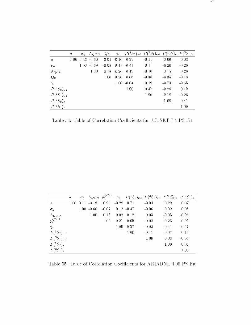
51

a �q �QCD Q0 s P (1S0)ud P (3S1)ud P (1S0)s P (3S1)s

a 1.00 0.33 -0.60 0.01 -0.10 0.27 -0.11 0.06 0.03

�q 1.00 -0.69 -0.08 0.43 -0.41 0.11 -0.26 -0.29

�QCD 1.00 0.18 -0.26 0.19 -0.10 0.15 0.20

Q0 1.00 0.20 0.06 -0.38 -0.35 -0.13

s 1.00 -0.04 0.19 -0.73 -0.65

P (1S0)ud 1.00 0.37 -0.29 0.12

P (3S1)ud 1.00 -0.10 -0.26

P (1S0)s 1.00 0.41

P (3S1)s 1.00

Table 54: Table of Correlation Coe�cients for JETSET 7.4 PS Fit

a �q �QCD pQCDt s P (1S0)ud P (3S1)ud P (1S0)s P (3S1)s

a 1.00 0.11 -0.18 0.90 -0.29 0.71 -0.04 0.29 0.07

�q 1.00 -0.60 -0.07 0.12 -0.47 -0.06 0.02 0.05

�QCD 1.00 0.16 0.02 0.18 0.03 -0.03 -0.06

pQCDt 1.00 -0.21 0.65 -0.02 0.26 0.05

s 1.00 -0.27 -0.02 -0.41 -0.47

P (1S0)ud 1.00 -0.11 -0.03 0.13

P (3S1)ud 1.00 0.08 -0.03

P (1S0)s 1.00 0.02

P (3S1)s 1.00

Table 55: Table of Correlation Coe�cients for ARIADNE 4.06 PS Fit

52

F Figures of Data and Model Comparisons

The �gures in this section compare corrected DELPHI data and identi�ed particlespectra to the following fragmentation models:

� JETSET 7.3 with DELPHI decays labeled JT 7.3 PS (full curves)� JETSET 7.4 with default decays labeled JT 7.4 PS (dashed curves)� ARIADNE 4.06 with DELPHI decays labeled AR 4.06 (dotted curves)� HERWIG 5.8 C with default decays labeled H 5.8 C (dot-dashed curves)� JETSET 7.4 ME with default decays labeled JT 7.4 ME (widely spaced dots)

The references for the identi�ed particle data can be found in table 7. The total correctionfactor for each distribution is shown in the upper inset. The lower insets of the plots showthe relative deviation of the models from the data. Also shown as a shaded area in theseinsets is the total experimental error obtained by adding quadratically the systematicand statistical error in each bin. The error should be interpreted like a statistical onestandard deviation uncertainty.

For the �p distributions of identi�ed K0, K�, p and �0 (Figs. 39, 40, 45, 46), we alsoshow separate plots comparing the models with each data set separately (ALEPH dashedcurve, DELPHI full curve, OPAL dotted curve).

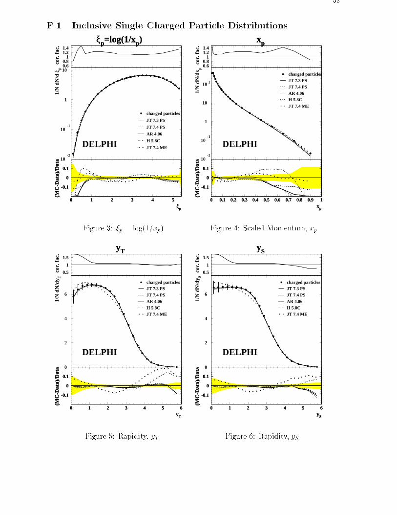
53

F.1 Inclusive Single Charged Particle Distributions

ξp=log(1/xp)

cor.

fac.

0.60.8

11.21.4

10-2

10-1

1

10

ξp=log(1/xp)

1/N

dN

/d ξ

p

DELPHI

charged particles

JT 7.3 PS

JT 7.4 PS

AR 4.06

H 5.8C

JT 7.4 ME

ξp

(MC

-Dat

a)/D

ata

-0.1

0

0.1

0 1 2 3 4 5ξp

(MC

-Dat

a)/D

ata

-0.1

0

0.1

0 1 2 3 4 5

Figure 3: �p = log(1=xp)

xp

cor.

fac.

0.60.8

11.21.4

10-2

10-1

1

10

10 2

xp

1/N

dN

/dx p

DELPHI

charged particlesJT 7.3 PSJT 7.4 PSAR 4.06H 5.8CJT 7.4 ME

xp

(MC

-Dat

a)/D

ata

-0.1

0

0.1

0 0.1 0.2 0.3 0.4 0.5 0.6 0.7 0.8 0.9 1xp

(MC

-Dat

a)/D

ata

-0.1

0

0.1

0 0.1 0.2 0.3 0.4 0.5 0.6 0.7 0.8 0.9 1

Figure 4: Scaled Momentum, xp

yT

cor.

fac.

0.5

1

1.5

0

2

4

6

yT

1/N

dN

/dy T

DELPHI

charged particlesJT 7.3 PSJT 7.4 PSAR 4.06H 5.8CJT 7.4 ME

yT

(MC

-Dat

a)/D

ata

-0.1

0

0.1

0 1 2 3 4 5 6yT

(MC

-Dat

a)/D

ata

-0.1

0

0.1

0 1 2 3 4 5 6

Figure 5: Rapidity, yT

yS

cor.

fac.

0.5

1

1.5

0

2

4

6

yS

1/N

dN

/dy S

DELPHI

charged particlesJT 7.3 PSJT 7.4 PSAR 4.06H 5.8CJT 7.4 ME

yS

(MC

-Dat

a)/D

ata

-0.1

0

0.1

0 1 2 3 4 5 6yS

(MC

-Dat

a)/D

ata

-0.1

0

0.1

0 1 2 3 4 5 6

Figure 6: Rapidity, yS

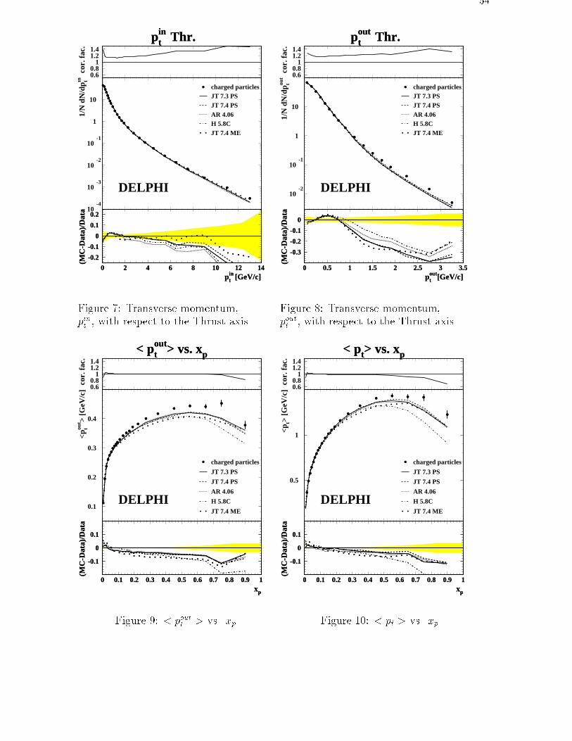
54

ptin

Thr.

cor.

fac.

0.60.8

11.21.4

10-4

10-3

10-2

10-1

1

10

ptin

Thr.

1/N

dN

/dp tin

DELPHI

charged particlesJT 7.3 PSJT 7.4 PSAR 4.06H 5.8CJT 7.4 ME

ptin [GeV/c]

(MC

-Dat

a)/D

ata

-0.2

-0.1

0

0.1

0.2

0 2 4 6 8 10 12 14pt

in [GeV/c]

(MC

-Dat

a)/D

ata

-0.2

-0.1

0

0.1

0.2

0 2 4 6 8 10 12 14

Figure 7: Transverse momentum,pint , with respect to the Thrust axis

ptout

Thr.

cor.

fac.

0.60.8

11.21.4

10-2

10-1

1

10

ptout

Thr.

1/N

dN

/dp tou

t

DELPHI

charged particlesJT 7.3 PSJT 7.4 PSAR 4.06H 5.8CJT 7.4 ME

ptout[GeV/c]

(MC

-Dat

a)/D

ata

-0.3

-0.2

-0.1

0

0 0.5 1 1.5 2 2.5 3 3.5pt

out[GeV/c](M

C-D

ata)

/Dat

a

-0.3

-0.2

-0.1

0

0 0.5 1 1.5 2 2.5 3 3.5

Figure 8: Transverse momentum,poutt , with respect to the Thrust axis

< ptout> vs. xp

cor.

fac.

0.60.8

11.21.4

0.1

0.2

0.3

0.4

< ptout> vs. xp

<p tou

t > [G

eV/c

]

DELPHI

charged particles

JT 7.3 PS

JT 7.4 PS

AR 4.06

H 5.8C

JT 7.4 ME

xp

(MC

-Dat

a)/D

ata

-0.1

0

0.1

0 0.1 0.2 0.3 0.4 0.5 0.6 0.7 0.8 0.9 1xp

(MC

-Dat

a)/D

ata

-0.1

0

0.1

0 0.1 0.2 0.3 0.4 0.5 0.6 0.7 0.8 0.9 1

Figure 9: < poutt > vs. xp

< pt> vs. xp

cor.

fac.

0.60.8

11.21.4

0.5

1

< pt> vs. xp

<p t>

[GeV

/c]

DELPHI

charged particles

JT 7.3 PS

JT 7.4 PS

AR 4.06

H 5.8C

JT 7.4 ME

xp

(MC

-Dat

a)/D

ata

-0.1

0

0.1

0 0.1 0.2 0.3 0.4 0.5 0.6 0.7 0.8 0.9 1xp

(MC

-Dat

a)/D

ata

-0.1

0

0.1

0 0.1 0.2 0.3 0.4 0.5 0.6 0.7 0.8 0.9 1

Figure 10: < pt > vs. xp

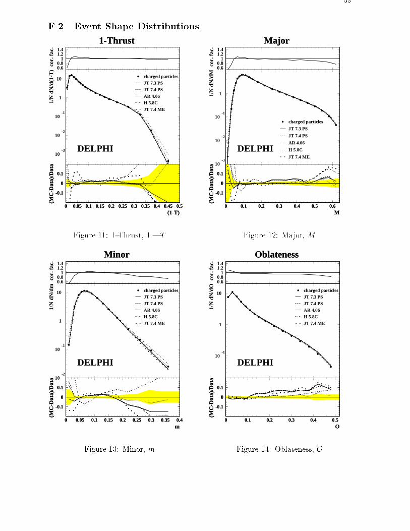
55

F.2 Event Shape Distributions

1-Thrustco

r. fa

c.

0.60.8

11.21.4

10-3

10-2

10-1

1

10

1-Thrust1/

N d

N/d

(1-T

)

DELPHI

charged particlesJT 7.3 PSJT 7.4 PSAR 4.06H 5.8CJT 7.4 ME

(1-T)

(MC

-Dat

a)/D

ata

-0.1

0

0.1

0 0.05 0.1 0.15 0.2 0.25 0.3 0.35 0.4 0.45 0.5(1-T)

(MC

-Dat

a)/D

ata

-0.1

0

0.1

0 0.05 0.1 0.15 0.2 0.25 0.3 0.35 0.4 0.45 0.5

Figure 11: 1-Thrust, 1� T

Major

cor.

fac.

0.60.8

11.21.4

10-3

10-2

10-1

1

Major

1/N

dN

/dM

DELPHI

charged particles

JT 7.3 PS

JT 7.4 PS

AR 4.06

H 5.8C

JT 7.4 ME

M(M

C-D

ata)

/Dat

a

-0.1

0

0.1

0 0.1 0.2 0.3 0.4 0.5 0.6M

(MC

-Dat

a)/D

ata

-0.1

0

0.1

0 0.1 0.2 0.3 0.4 0.5 0.6

Figure 12: Major, M

Minor

cor.

fac.

0.60.8

11.21.4

10-2

10-1

1

10

Minor

1/N

dN

/dm

DELPHI

charged particlesJT 7.3 PSJT 7.4 PSAR 4.06H 5.8CJT 7.4 ME

m

(MC

-Dat

a)/D

ata

-0.1

0

0.1

0 0.05 0.1 0.15 0.2 0.25 0.3 0.35 0.4m

(MC

-Dat

a)/D

ata

-0.1

0

0.1

0 0.05 0.1 0.15 0.2 0.25 0.3 0.35 0.4

Figure 13: Minor, m

Oblateness

cor.

fac.

0.60.8

11.21.4

10-1

1

10

Oblateness

1/N

dN

/dO

DELPHI

charged particlesJT 7.3 PSJT 7.4 PSAR 4.06H 5.8CJT 7.4 ME

O

(MC

-Dat

a)/D

ata

-0.1

0

0.1

0 0.1 0.2 0.3 0.4 0.5O

(MC

-Dat

a)/D

ata

-0.1

0

0.1

0 0.1 0.2 0.3 0.4 0.5

Figure 14: Oblateness, O

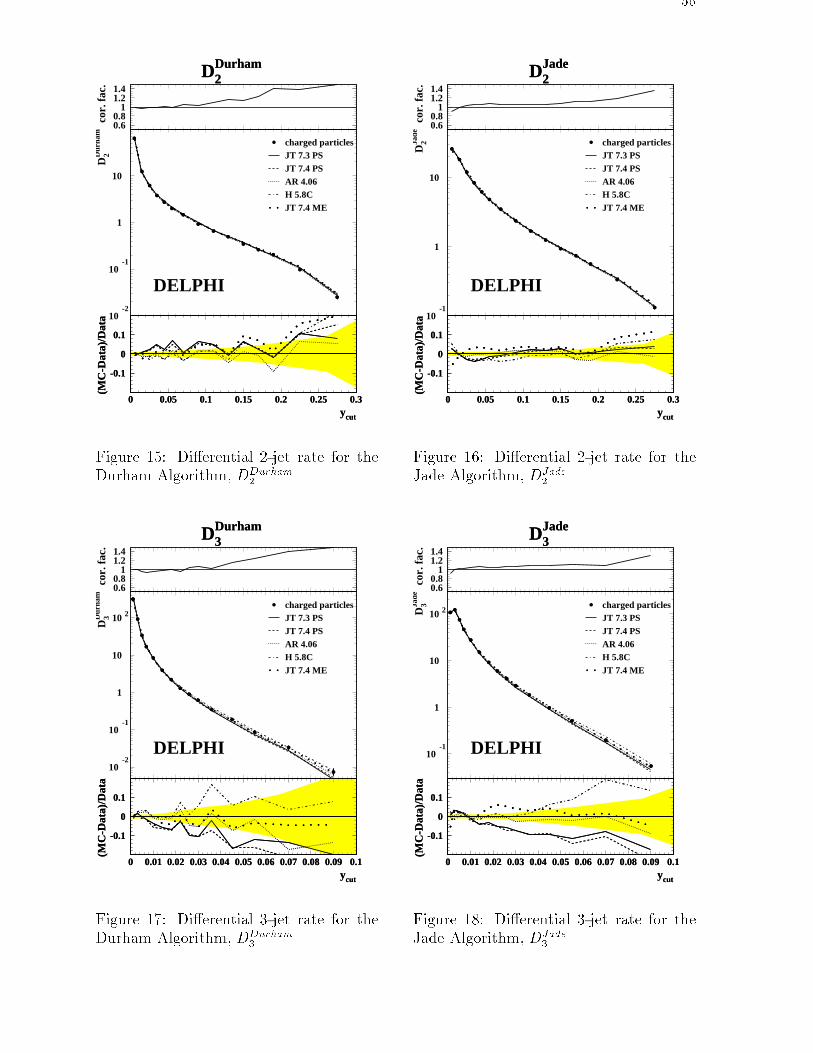
56

D2Durham

cor.

fac.

0.60.8

11.21.4

10-2

10-1

1

10

D2Durham

D2D

urha

m

DELPHI

charged particlesJT 7.3 PSJT 7.4 PSAR 4.06H 5.8CJT 7.4 ME

ycut

(MC

-Dat

a)/D

ata

-0.1

0

0.1

0 0.05 0.1 0.15 0.2 0.25 0.3ycut

(MC

-Dat

a)/D

ata

-0.1

0

0.1

0 0.05 0.1 0.15 0.2 0.25 0.3

Figure 15: Di�erential 2-jet rate for theDurham Algorithm, DDurham

2

D2Jade

cor.

fac.

0.60.8

11.21.4

10-1

1

10

D2Jade

D2Ja

de

DELPHI

charged particlesJT 7.3 PSJT 7.4 PSAR 4.06H 5.8CJT 7.4 ME

ycut(M

C-D

ata)

/Dat

a

-0.1

0

0.1

0 0.05 0.1 0.15 0.2 0.25 0.3ycut(M

C-D

ata)

/Dat

a

-0.1

0

0.1

0 0.05 0.1 0.15 0.2 0.25 0.3

Figure 16: Di�erential 2-jet rate for theJade Algorithm, DJade

2

D3Durham

cor.

fac.

0.60.8

11.21.4

10-2

10-1

1

10

10 2

D3Durham

D3D

urha

m

DELPHI

charged particlesJT 7.3 PSJT 7.4 PSAR 4.06H 5.8CJT 7.4 ME

ycut

(MC

-Dat

a)/D

ata

-0.1

0

0.1

0 0.01 0.02 0.03 0.04 0.05 0.06 0.07 0.08 0.09 0.1ycut

(MC

-Dat

a)/D

ata

-0.1

0

0.1

0 0.01 0.02 0.03 0.04 0.05 0.06 0.07 0.08 0.09 0.1

Figure 17: Di�erential 3-jet rate for theDurham Algorithm, DDurham

3

D3Jade

cor.

fac.

0.60.8

11.21.4

10-1

1

10

10 2

D3Jade

D3Ja

de

DELPHI

charged particlesJT 7.3 PSJT 7.4 PSAR 4.06H 5.8CJT 7.4 ME

ycut

(MC

-Dat

a)/D

ata

-0.1

0

0.1

0 0.01 0.02 0.03 0.04 0.05 0.06 0.07 0.08 0.09 0.1ycut

(MC

-Dat

a)/D

ata

-0.1

0

0.1

0 0.01 0.02 0.03 0.04 0.05 0.06 0.07 0.08 0.09 0.1

Figure 18: Di�erential 3-jet rate for theJade Algorithm, DJade

3

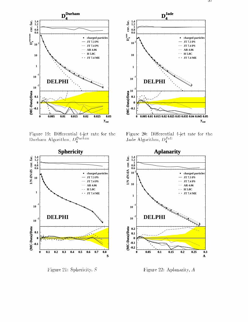
57

D4Durham

cor.

fac.

0.60.8

11.21.4

10-2

10-1

1

10

10 2

D4Durham

D4D

urha

m

DELPHI

charged particlesJT 7.3 PSJT 7.4 PSAR 4.06H 5.8CJT 7.4 ME

ycut

(MC

-Dat

a)/D

ata

-0.1

0

0.1

0 0.005 0.01 0.015 0.02 0.025 0.03ycut

(MC

-Dat

a)/D

ata

-0.1

0

0.1

0 0.005 0.01 0.015 0.02 0.025 0.03

Figure 19: Di�erential 4-jet rate for theDurham Algorithm, DDurham

4

D4Jade

cor.

fac.

0.60.8

11.21.4

10-2

10-1

1

10

10 2

D4Jade

D4Ja

de

DELPHI

charged particlesJT 7.3 PSJT 7.4 PSAR 4.06H 5.8CJT 7.4 ME

ycut

(MC

-Dat

a)/D

ata

-0.1

0

0.1

0 0.005 0.01 0.015 0.02 0.025 0.03 0.035 0.04 0.045 0.05ycut

(MC

-Dat

a)/D

ata

-0.1

0

0.1

0 0.005 0.01 0.015 0.02 0.025 0.03 0.035 0.04 0.045 0.05

Figure 20: Di�erential 4-jet rate for theJade Algorithm, DJade

4

Sphericity

cor.

fac.

0.60.8

11.21.4

10-2

10-1

1

10

Sphericity

1/N

dN

/dS

DELPHI

charged particlesJT 7.3 PSJT 7.4 PSAR 4.06H 5.8CJT 7.4 ME

S

(MC

-Dat

a)/D

ata

-0.1

0

0.1

0 0.1 0.2 0.3 0.4 0.5 0.6 0.7 0.8S

(MC

-Dat

a)/D

ata

-0.1

0

0.1

0 0.1 0.2 0.3 0.4 0.5 0.6 0.7 0.8

Figure 21: Sphericity, S

Aplanarity

cor.

fac.

0.60.8

11.21.4

10-2

10-1

1

10

10 2

Aplanarity

1/N

dN

/dA

DELPHI

charged particlesJT 7.3 PSJT 7.4 PSAR 4.06H 5.8CJT 7.4 ME

A

(MC

-Dat

a)/D

ata

-0.2

-0.1

0

0.1

0.2

0 0.05 0.1 0.15 0.2 0.25 0.3A

(MC

-Dat

a)/D

ata

-0.2

-0.1

0

0.1

0.2

0 0.05 0.1 0.15 0.2 0.25 0.3

Figure 22: Aplanarity, A

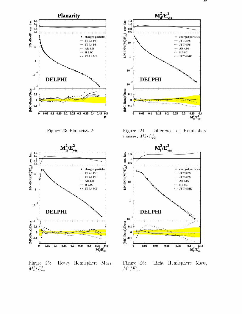
58

Planarity

cor.

fac.

0.60.8

11.21.4

10-2

10-1

1

10

Planarity

1/N

dN

/dP

DELPHI

charged particlesJT 7.3 PSJT 7.4 PSAR 4.06H 5.8CJT 7.4 ME

P

(MC

-Dat

a)/D

ata

-0.1

0

0.1

0 0.05 0.1 0.15 0.2 0.25 0.3 0.35 0.4 0.45 0.5P

(MC

-Dat

a)/D

ata

-0.1

0

0.1

0 0.05 0.1 0.15 0.2 0.25 0.3 0.35 0.4 0.45 0.5

Figure 23: Planarity, P

M2d/E

2vis

cor.

fac.

0.60.8

11.21.4

10-2

10-1

1

10

M2d/E

2vis

1/N

dN

/d(M

2 d/E

2 vis)

DELPHI

charged particlesJT 7.3 PSJT 7.4 PSAR 4.06H 5.8CJT 7.4 ME

M2d/E

2vis

(MC

-Dat

a)/D

ata

-0.1

0

0.1

0 0.05 0.1 0.15 0.2 0.25 0.3 0.35 0.4M2

d/E2vis

(MC

-Dat

a)/D

ata

-0.1

0

0.1

0 0.05 0.1 0.15 0.2 0.25 0.3 0.35 0.4

Figure 24: Di�erence of Hemispheremasses, M2

d=E2

vis

M2h/E

2vis

cor.

fac.

0.60.8

11.21.4

10-2

10-1

1

10

M2h/E

2vis

1/N

dN

/d(M

2 h/E

2 vis)

DELPHI

charged particlesJT 7.3 PSJT 7.4 PSAR 4.06H 5.8CJT 7.4 ME

M2h/E

2vis

(MC

-Dat

a)/D

ata

-0.1

0

0.1

0 0.05 0.1 0.15 0.2 0.25 0.3 0.35 0.4M2

h/E2vis

(MC

-Dat

a)/D

ata

-0.1

0

0.1

0 0.05 0.1 0.15 0.2 0.25 0.3 0.35 0.4

Figure 25: Heavy Hemisphere Mass,M2

h=E2

vis

M2l /E

2vis

cor.

fac.

0.5

1

1.5

10-1

1

10

M2l /E

2vis

1/N

dN

/d(M

2 l/E

2 vis)

DELPHI

charged particlesJT 7.3 PSJT 7.4 PSAR 4.06H 5.8CJT 7.4 ME

M2l /E

2vis

(MC

-Dat

a)/D

ata

-0.1

0

0.1

0 0.02 0.04 0.06 0.08 0.1 0.12M2

l /E2vis

(MC

-Dat

a)/D

ata

-0.1

0

0.1

0 0.02 0.04 0.06 0.08 0.1 0.12

Figure 26: Light Hemisphere Mass,M2

l =E2

vis

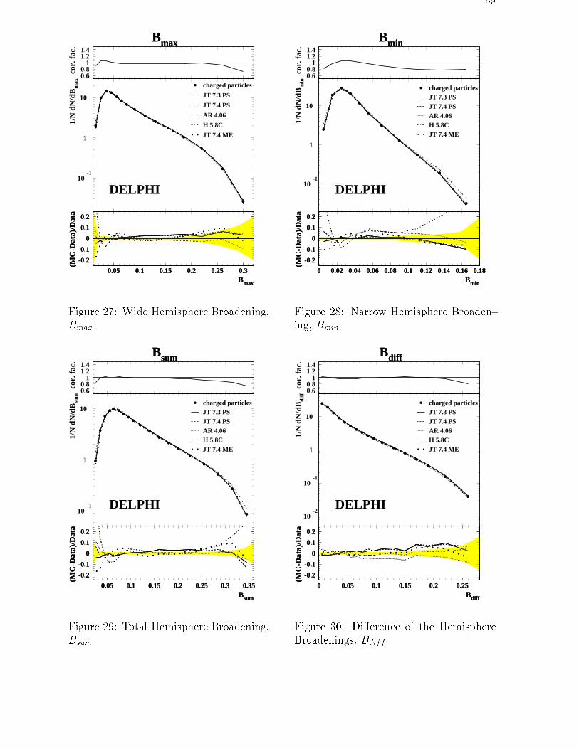
59

Bmax

cor.

fac.

0.60.8

11.21.4

10-1

1

10

Bmax

1/N

dN

/dB

max

DELPHI

charged particles

JT 7.3 PS

JT 7.4 PS

AR 4.06

H 5.8C

JT 7.4 ME

Bmax

(MC

-Dat

a)/D

ata

-0.2

-0.1

0

0.1

0.2

0.05 0.1 0.15 0.2 0.25 0.3Bmax

(MC

-Dat

a)/D

ata

-0.2

-0.1

0

0.1

0.2

0.05 0.1 0.15 0.2 0.25 0.3

Figure 27: Wide Hemisphere Broadening,Bmax

Bmin

cor.

fac.

0.60.8

11.21.4

10-1

1

10

Bmin

1/N

dN

/dB

min

DELPHI

charged particlesJT 7.3 PSJT 7.4 PSAR 4.06H 5.8CJT 7.4 ME

Bmin

(MC

-Dat

a)/D

ata

-0.2

-0.1

0

0.1

0.2

0 0.02 0.04 0.06 0.08 0.1 0.12 0.14 0.16 0.18Bmin

(MC

-Dat

a)/D

ata

-0.2

-0.1

0

0.1

0.2

0 0.02 0.04 0.06 0.08 0.1 0.12 0.14 0.16 0.18

Figure 28: Narrow Hemisphere Broaden-ing, Bmin

Bsum

cor.

fac.

0.60.8

11.21.4

10-1

1

10

Bsum

1/N

dN

/dB

sum

DELPHI

charged particlesJT 7.3 PSJT 7.4 PSAR 4.06H 5.8CJT 7.4 ME

Bsum

(MC

-Dat

a)/D

ata

-0.2

-0.1

0

0.1

0.2

0.05 0.1 0.15 0.2 0.25 0.3 0.35Bsum

(MC

-Dat

a)/D

ata

-0.2

-0.1

0

0.1

0.2

0.05 0.1 0.15 0.2 0.25 0.3 0.35

Figure 29: Total Hemisphere Broadening,Bsum

Bdiff

cor.

fac.

0.60.8

11.21.4

10-2

10-1

1

10

Bdiff

1/N

dN

/dB

diff

DELPHI

charged particlesJT 7.3 PSJT 7.4 PSAR 4.06H 5.8CJT 7.4 ME

Bdiff

(MC

-Dat

a)/D

ata

-0.2

-0.1

0

0.1

0.2

0 0.05 0.1 0.15 0.2 0.25Bdiff

(MC

-Dat

a)/D

ata

-0.2

-0.1

0

0.1

0.2

0 0.05 0.1 0.15 0.2 0.25

Figure 30: Di�erence of the HemisphereBroadenings, Bdiff

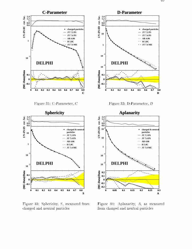
60

C-Parameter

cor.

fac.

0.60.8

11.21.4

10-1

1

C-Parameter

1/N

dN

/dC

DELPHI

charged particlesJT 7.3 PSJT 7.4 PSAR 4.06H 5.8CJT 7.4 ME

C

(MC

-Dat

a)/D

ata

-0.1

0

0.1

0 0.1 0.2 0.3 0.4 0.5 0.6 0.7 0.8 0.9C

(MC

-Dat

a)/D

ata

-0.1

0

0.1

0 0.1 0.2 0.3 0.4 0.5 0.6 0.7 0.8 0.9

Figure 31: C-Parameter, C

D-Parameter

cor.

fac.

0.60.8

11.21.4

10-2

10-1

1

10

D-Parameter

1/N

dN

/dD

DELPHI

charged particlesJT 7.3 PSJT 7.4 PSAR 4.06H 5.8CJT 7.4 ME

D

(MC

-Dat

a)/D

ata

-0.1

0

0.1

0 0.1 0.2 0.3 0.4 0.5 0.6 0.7 0.8D

(MC

-Dat

a)/D

ata

-0.1

0

0.1

0 0.1 0.2 0.3 0.4 0.5 0.6 0.7 0.8

Figure 32: D-Parameter, D

Sphericity

cor.

fac.

0.60.8

11.21.4

10-2

10-1

1

10

Sphericity

1/N

dN

/dS

DELPHI

charged & neutralparticlesJT 7.3 PSJT 7.4 PSAR 4.06H 5.8CJT 7.4 ME

S

(MC

-Dat

a)/D

ata

-0.1

0

0.1

0 0.1 0.2 0.3 0.4 0.5 0.6 0.7 0.8S

(MC

-Dat

a)/D

ata

-0.1

0

0.1

0 0.1 0.2 0.3 0.4 0.5 0.6 0.7 0.8

Figure 33: Sphericity, S, measured fromcharged and neutral particles

Aplanarity

cor.

fac.

0.60.8

11.21.4

10-2

10-1

1

10

10 2

Aplanarity

1/N

dN

/dA

DELPHI

charged & neutralparticlesJT 7.3 PSJT 7.4 PSAR 4.06H 5.8CJT 7.4 ME

A

(MC

-Dat

a)/D

ata

-0.2

-0.1

0

0.1

0.2

0 0.05 0.1 0.15 0.2 0.25 0.3A

(MC

-Dat

a)/D

ata

-0.2

-0.1

0

0.1

0.2

0 0.05 0.1 0.15 0.2 0.25 0.3

Figure 34: Aplanarity, A, as measuredfrom charged and neutral particles

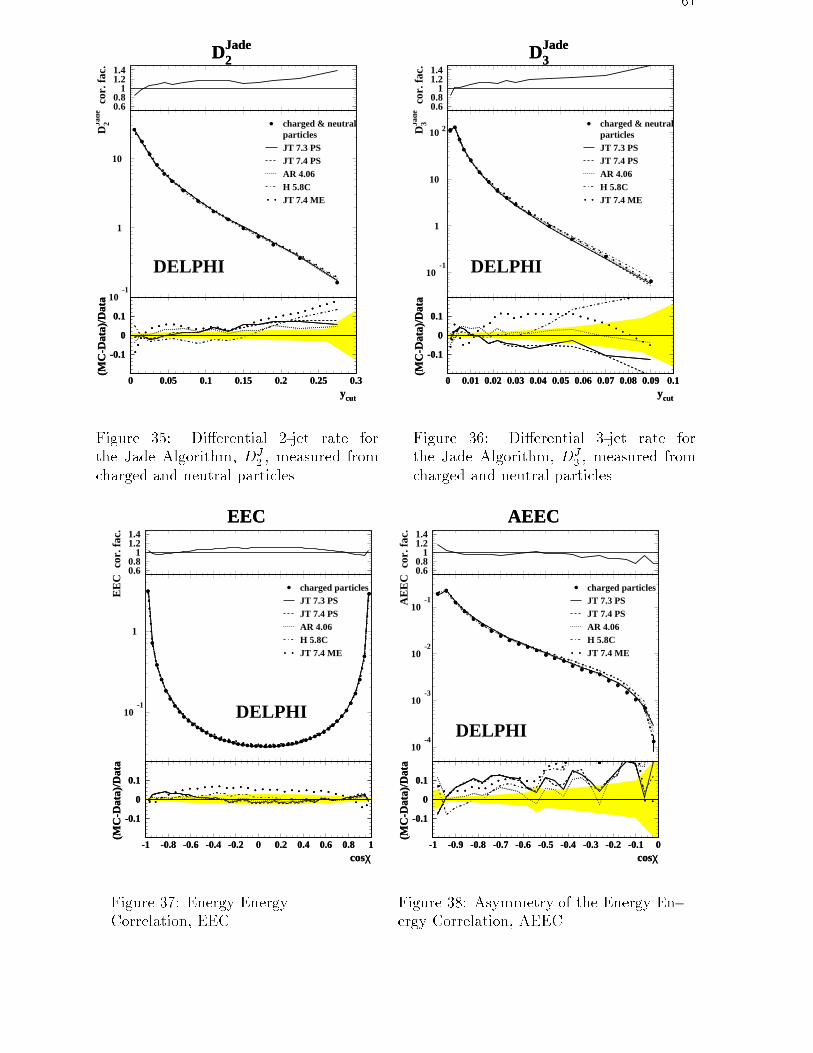
61

D2Jade

cor.

fac.

0.60.8

11.21.4

10-1

1

10

D2Jade

D2Ja

de

DELPHI

charged & neutralparticlesJT 7.3 PSJT 7.4 PSAR 4.06H 5.8CJT 7.4 ME

ycut

(MC

-Dat

a)/D

ata

-0.1

0

0.1

0 0.05 0.1 0.15 0.2 0.25 0.3ycut

(MC

-Dat

a)/D

ata

-0.1

0

0.1

0 0.05 0.1 0.15 0.2 0.25 0.3

Figure 35: Di�erential 2-jet rate forthe Jade Algorithm, DJ

2, measured from

charged and neutral particles

D3Jade

cor.

fac.

0.60.8

11.21.4

10-1

1

10

10 2

D3Jade

D3Ja

de

DELPHI

charged & neutralparticlesJT 7.3 PSJT 7.4 PSAR 4.06H 5.8CJT 7.4 ME

ycut

(MC

-Dat

a)/D

ata

-0.1

0

0.1

0 0.01 0.02 0.03 0.04 0.05 0.06 0.07 0.08 0.09 0.1ycut

(MC

-Dat

a)/D

ata

-0.1

0

0.1

0 0.01 0.02 0.03 0.04 0.05 0.06 0.07 0.08 0.09 0.1

Figure 36: Di�erential 3-jet rate forthe Jade Algorithm, DJ

3, measured from

charged and neutral particles

EEC

cor.

fac.

0.60.8

11.21.4

10-1

1

EEC

EE

C

DELPHI

charged particlesJT 7.3 PSJT 7.4 PSAR 4.06H 5.8CJT 7.4 ME

cosχ

(MC

-Dat

a)/D

ata

-0.1

0

0.1

-1 -0.8 -0.6 -0.4 -0.2 0 0.2 0.4 0.6 0.8 1cosχ

(MC

-Dat

a)/D

ata

-0.1

0

0.1

-1 -0.8 -0.6 -0.4 -0.2 0 0.2 0.4 0.6 0.8 1

Figure 37: Energy EnergyCorrelation, EEC

AEEC

cor.

fac.

0.60.8

11.21.4

10-4

10-3

10-2

10-1

AEEC

AE

EC

DELPHI

charged particlesJT 7.3 PSJT 7.4 PSAR 4.06H 5.8CJT 7.4 ME

cosχ

(MC

-Dat

a)/D

ata

-0.1

0

0.1

-1 -0.9 -0.8 -0.7 -0.6 -0.5 -0.4 -0.3 -0.2 -0.1 0cosχ

(MC

-Dat

a)/D

ata

-0.1

0

0.1

-1 -0.9 -0.8 -0.7 -0.6 -0.5 -0.4 -0.3 -0.2 -0.1 0

Figure 38: Asymmetry of the Energy En-ergy Correlation, AEEC

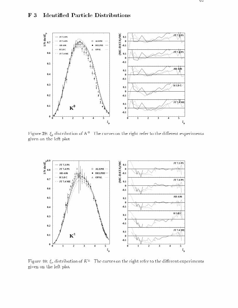
62

F.3 Identi�ed Particle Distributions

0

0.1

0.2

0.3

0.4

0.5

0.6

0.7

0 1 2 3 4 5

ξp

1/N

dn/

dξp

ALEPH

DELPHI

OPAL

JT 7.3 PS

JT 7.4 PS

AR 4.06

H 5.8 C

JT 7.4 ME

K0

(MC

-DA

TA

)/M

C JT 7.3 PS

-0.1

0

0.1

-0.1

0

0.1JT 7.4 PS

-0.1

0

0.1AR 4.06

-0.1

0

0.1H 5.8 C

-0.1

0

0.1

0 1 2 3 4 5

ξp

JT 7.4 ME

Figure 39: �p distribution ofK0. The curves on the right refer to the di�erent experimentsgiven on the left plot.

0

0.1

0.2

0.3

0.4

0.5

0.6

0.7

0.8

0.9

0 1 2 3 4 5

ξp

1/N

dn/

dξp

ALEPH

DELPHI

OPAL

JT 7.3 PS

JT 7.4 PS

AR 4.06

H 5.8 C

JT 7.4 ME

K±

(MC

-DA

TA

)/M

C JT 7.3 PS

-0.1

0

0.1

-0.1

0

0.1JT 7.4 PS

-0.1

0

0.1AR 4.06

-0.1

0

0.1H 5.8 C

-0.1

0

0.1

0 1 2 3 4 5

ξp

JT 7.4 ME

Figure 40: �p distribution ofK�. The curves on the right refer to the di�erent experimentsgiven on the left plot.

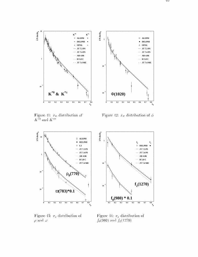
63

10-1

1

10

0 0.1 0.2 0.3 0.4 0.5 0.6 0.7 0.8xp

1/N

dn/

dxp

K *±K*0

ALEPH

DELPHI

OPAL

JT 7.3 PS

JT 7.4 PS

AR 4.06

H 5.8 C

JT 7.4 ME

K*0 & K *±

Figure 41: xE distribution ofK�0 and K��

10-2

10-1

1

0 0.1 0.2 0.3 0.4 0.5 0.6 0.7 0.8xE

1/N

dn/

dxE

ALEPH

DELPHI

OPAL

JT 7.3 PS

JT 7.4 PS

AR 4.06

H 5.8 C

JT 7.4 ME

Φ(1020)

Figure 42: xE distribution of �

10-2

10-1

1

10

0 0.1 0.2 0.3 0.4 0.5 0.6 0.7 0.8xp

1/N

dn/

dxp

ALEPH

DELPHI

L3

JT 7.3 PS

JT 7.4 PS

AR 4.06

H 5.8 C

JT 7.4 ME

ρ0(770)

ω(783)*0.1

Figure 43: xp distribution of� and !

10-2

10-1

1

0.1 0.2 0.3 0.4 0.5 0.6 0.7 0.8xp

1/N

dn/

dxp

f0 f2

DELPHI

JT 7.3 PS

JT 7.4 PS

AR 4.06

H 5.8 C

JT 7.4 ME

f2(1270)

f0(980) * 0.1

Figure 44: xp distribution off0(980) and f2(1270)

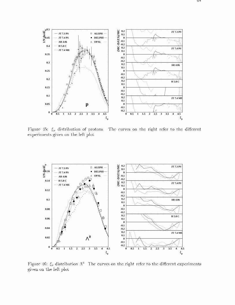
64

0

0.05

0.1

0.15

0.2

0.25

0.3

0.35

0.4

0.45

0.5

0 0.5 1 1.5 2 2.5 3 3.5 4 4.5

ξp

1/N

dn/

dξp

ALEPH

DELPHI

OPAL

JT 7.3 PS

JT 7.4 PS

AR 4.06

H 5.8 C

JT 7.4 ME

p

(MC

-DA

TA

)/M

C JT 7.3 PS

-0.2-0.1

00.10.2

-0.2-0.1

00.10.2 JT 7.4 PS

-0.2-0.1

00.10.2 AR 4.06

-0.2-0.1

00.10.2 H 5.8 C

-0.2-0.1

00.10.2

0 0.5 1 1.5 2 2.5 3 3.5 4 4.5

ξp

JT 7.4 ME

Figure 45: �p distribution of protons. The curves on the right refer to the di�erentexperiments given on the left plot.

0

0.02

0.04

0.06

0.08

0.1

0.12

0.14

0.16

0 0.5 1 1.5 2 2.5 3 3.5 4 4.5

ξp

1/N

dn/

dξp

ALEPH

DELPHI

OPAL

JT 7.3 PS

JT 7.4 PS

AR 4.06

H 5.8 C

JT 7.4 ME

Λ0

(MC

-DA

TA

)/M

C JT 7.3 PS

-0.2-0.1

00.10.2

-0.2-0.1

00.10.2 JT 7.4 PS

-0.2-0.1

00.10.2 AR 4.06

-0.2-0.1

00.10.2 H 5.8 C

-0.2-0.1

00.10.2

0 0.5 1 1.5 2 2.5 3 3.5 4 4.5

ξp

JT 7.4 ME

Figure 46: �p distribution �0. The curves on the right refer to the di�erent experimentsgiven on the left plot.

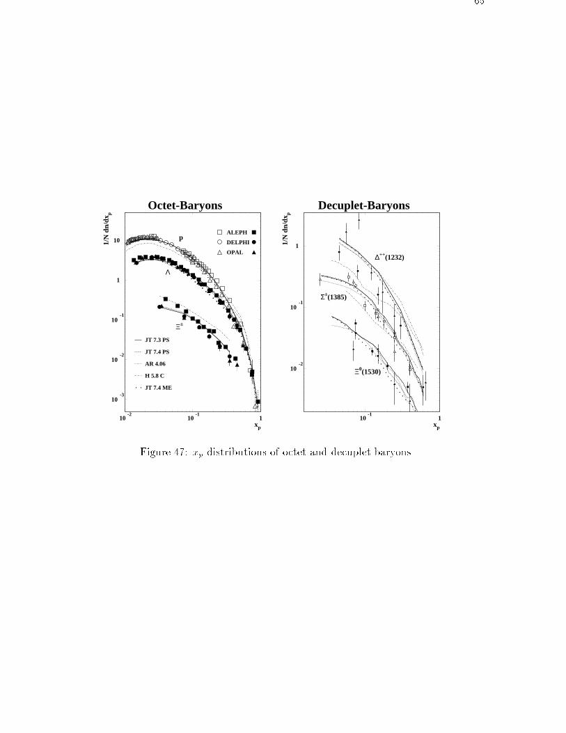
65

Octet-Baryons

10-3

10-2

10-1

1

10

10-2

10-1

1xp

1/N

dn/

dxp

p

Λ

Ξ±

ALEPH

DELPHI

OPAL

JT 7.3 PS

JT 7.4 PS

AR 4.06

H 5.8 C

JT 7.4 ME

Decuplet-Baryons

10-2

10-1

1

10-1

1xp

1/N

dn/

dxp

∆++(1232)

Σ±(1385)

Ξ0(1530)

Figure 47: xp distributions of octet and decuplet baryons

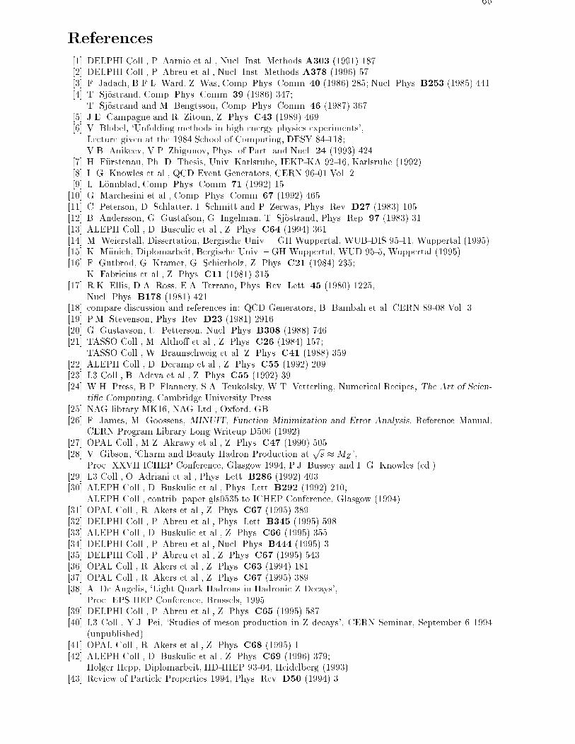
66

References

[1] DELPHI Coll., P. Aarnio et al., Nucl. Inst. Methods A303 (1991) 187.[2] DELPHI Coll., P. Abreu et al., Nucl. Inst. Methods A378 (1996) 57.[3] F. Jadach, B.F.L. Ward, Z. Was, Comp. Phys. Comm. 40 (1986) 285; Nucl. Phys. B253 (1985) 441.[4] T. Sj�ostrand, Comp. Phys. Comm. 39 (1986) 347;

T. Sj�ostrand and M. Bengtsson, Comp. Phys. Comm. 46 (1987) 367.[5] J.E. Campagne and R. Zitoun, Z. Phys. C43 (1989) 469.[6] V. Blobel, `Unfolding methods in high energy physics experiments',

Lecture given at the 1984 School of Computing, DESY 84-118;V.B. Anikeev, V.P. Zhigunov, Phys. of Part. and Nucl. 24 (1993) 424.

[7] H. F�urstenau, Ph. D. Thesis, Univ. Karlsruhe, IEKP-KA 92-16, Karlsruhe (1992).[8] I. G. Knowles et al., QCD Event Generators, CERN 96-01 Vol. 2.[9] L. L�onnblad, Comp. Phys. Comm. 71 (1992) 15.[10] G. Marchesini et al., Comp. Phys. Comm. 67 (1992) 465.[11] C. Peterson, D. Schlatter, I. Schmitt and P. Zerwas, Phys. Rev. D27 (1983) 105.[12] B. Andersson, G. Gustafson, G. Ingelman, T. Sj�ostrand, Phys. Rep. 97 (1983) 31.[13] ALEPH Coll., D. Busculic et al., Z. Phys. C64 (1994) 361.[14] M. Weierstall, Dissertation, Bergische Univ. { GH Wuppertal, WUB-DIS 95-11, Wuppertal (1995).[15] K. M�unich, Diplomarbeit, Bergische Univ. { GH Wuppertal, WUD 95-5, Wuppertal (1995).[16] F. Gutbrod, G. Kramer, G. Schierholz, Z. Phys. C21 (1984) 235;

K. Fabricius et al., Z. Phys. C11 (1981) 315.[17] R.K. Ellis, D.A. Ross, E.A. Terrano, Phys. Rev. Lett. 45 (1980) 1225,

Nucl. Phys. B178 (1981) 421.[18] compare discussion and references in: QCD Generators, B. Bambah et al. CERN 89-08 Vol. 3.[19] P.M. Stevenson, Phys. Rev. D23 (1981) 2916.[20] G. Gustavson, U. Petterson, Nucl. Phys. B308 (1988) 746.[21] TASSO Coll., M. Altho� et al., Z. Phys. C26 (1984) 157;

TASSO Coll., W. Braunschweig et al. Z. Phys. C41 (1988) 359.[22] ALEPH Coll., D. Decamp et al., Z. Phys. C55 (1992) 209.[23] L3 Coll., B. Adeva et al., Z. Phys. C55 (1992) 39.[24] W.H. Press, B.P. Flannery, S.A. Teukolsky, W.T. Vetterling, Numerical Recipes, The Art of Scien-

ti�c Computing, Cambridge University Press.[25] NAG library MK16, NAG Ltd., Oxford, GB.[26] F. James, M. Goossens, MINUIT, Function Minimization and Error Analysis, Reference Manual,

CERN Program Library Long Writeup D506 (1992).[27] OPAL Coll., M.Z. Akrawy et al., Z. Phys. C47 (1990) 505.[28] V. Gibson, `Charm and Beauty Hadron Production at

ps �MZ ',

Proc. XXVII ICHEP Conference, Glasgow 1994, P.J. Bussey and I. G. Knowles (ed.)[29] L3 Coll., O. Adriani et al., Phys. Lett. B286 (1992) 403.[30] ALEPH Coll., D. Buskulic et al., Phys. Lett. B292 (1992) 210;

ALEPH Coll., contrib. paper gls0535 to ICHEP Conference, Glasgow (1994).[31] OPAL Coll., R. Akers et al., Z. Phys. C67 (1995) 389.[32] DELPHI Coll., P. Abreu et al., Phys. Lett. B345 (1995) 598.[33] ALEPH Coll., D. Buskulic et al., Z. Phys. C66 (1995) 355.[34] DELPHI Coll., P. Abreu et al., Nucl. Phys. B444 (1995) 3.[35] DELPHI Coll., P. Abreu et al., Z. Phys. C67 (1995) 543.[36] OPAL Coll., R. Akers et al., Z. Phys. C63 (1994) 181.[37] OPAL Coll., R. Akers et al., Z. Phys. C67 (1995) 389.[38] A. De Angelis, `Light Quark Hadrons in Hadronic Z Decays',

Proc. EPS HEP Conference, Brussels, 1995.[39] DELPHI Coll., P. Abreu et al., Z. Phys. C65 (1995) 587.[40] L3 Coll., Y.J. Pei, `Studies of meson production in Z decays', CERN Seminar, September 6 1994

(unpublished).[41] OPAL Coll., R. Akers et al., Z. Phys. C68 (1995) 1.[42] ALEPH Coll., D. Buskulic et al., Z. Phys. C69 (1996) 379;

Holger Hepp, Diplomarbeit, HD-IHEP 93-04, Heidelberg (1993).[43] Review of Particle Properties 1994, Phys. Rev. D50 (1994) 3.

67

[44] OPAL Collaboration, M.Z. Akrawy Z. Phys. C47 (1990) 505;ALEPH Collaboration, D. Decamp et al., Phys. Lett. B273 (1991) 181;DELPHI Collaboration, A. Abreu et al., Z. Phys. C50 (1991) 185;OPAL Collaboration, P.D. Acton et al., Z. Phys. C53 (1992) 539.

[45] A. De Angelis, J. Phys. G19 (1993) 1233.[46] DELPHI Coll. P. Abreu et al., Phys. Lett. B347 (1995) 447.[47] DELPHI Coll., Contrib. paper eps0556 to EPS HEP Conference, Brussels (1995).[48] ALEPH Coll., D. Buskulic et al., Phys. Lett. B305 (1993) 415.[49] ALEPH Coll., Contrib. paper eps0419 to EPS HEP Conference, Brussels (1995).[50] ALEPH Coll., D. Buskulic et al., CERN-PPE 96-09 (1996).[51] S. Brandt et al., Phys. Lett. 12 (1964) 57;

E. Fahri, Phys. Rev. Lett. 39 (1977) 1587.[52] J.D. Bjorken, S. Brodsky, Phys. Rev. D1 (1970) 1416.[53] R.K. Ellis, D.A. Ross, A.E. Terrano, Nucl. Phys. B178 (1981) 421;

G. Parisi, Phys. Lett. B74 (1978) 65;J.F. Donohue, F.E. Low, S.Y. Pi, Phys. Rev. D20 (1979) 2759.

[54] L. Clavelli, Phys. Lett. B85 (1979) 111.[55] S. Catani, G. Turnock, B.R. Webber, Phys. Lett. B295 (1992) 269.[56] JADE Coll., W. Bartel et al., Z. Phys. C33 (1986) 23;

JADE Coll., S. Bethke et al., Phys. Lett. B213 (1988) 235.[57] S. Catani et al., Phys. Lett. B269 (1991) 432.[58] JADE Coll., N. Magnussen et al., Z. Phys. C49 (1991) 29.[59] C.L. Basham, L.S. Brown, S.D. Ellis, S.T. Love, Phys. Rev. D17 (1978) 2298,

Phys. Rev. Lett. 41 (1978) 1585, and Phys. Rev. D19 (1979) 2018.[60] DELPHI Coll., P. Abreu et al., Z. Phys. C63 (1994) 17;

DELPHI Coll., P. Abreu et al., Phys. Lett. B323 (1994) 242;DELPHI Coll., P. Abreu et al., Phys. Lett. B355 (1995) 415.