Tugas%20Kelompok%20PJ Fundamental%20RS

1

FUNDAMENTALS OF REMOTE

SENSING AND GIS

Shunji Murai Professor and Doctor of Engineering Institute of Industrial Science University of Tokyo, Japan Chair Professor, STAR Program Asian Institute of Technology, Thailand

2

Preface

Geographic Information System (GIS) has undergone a sort of boom all around the world in this decade as personal computers and engineering workstations have become available at reasonable prices. There were and are so many applications of GIS on various levels of central governments, local governments, utility service corporations, distribution service companies, car navigation systems, marketing strategies etc., but unfortunately not all them are successful. For successful GIS one of the keys is education and training, particularly with well organized teaching materials.

When I was teaching at the Asian Institute of Technology (AIT), Bangkok, Thailand for three years between 1992 and 1995, and also when I organized an international symposium on AM/FM GIS ASIA'95 in Bangkok, Thailand, August 1995, I was strongly requested by many people in the developing countries in Asia to publish a GIS text book, which is easily understandable in not only theory and principle but also in planning and application for a successful GIS. If you look at the exiting text books, most of them are not very much unified because some are collection of articles written by multiple authors, some are too thick and too expensive for educational purposes, some are too conceptual and theoretical background. Thus I have attempted to write an easily understood text with short explanation in not more than a page for each item on the left together with another page of only figures, tables and/or pictures on the right page, in organized manner.

In 1996 and 1997, I published GIS Work Book- Fundamental Course and Technical Course respectively with bi-lingal of English and Japanese. As some readers request me to publish only English version, I reedited the two volumes into a book with only English version.

I believe that this text book with its two parts ; "fundamental course" and "technical course" would be useful and helpful to not only students, trainees, engineers, salesmen but also to top managers or decision makers.

I would like to thank Mr. Minoru Tsuzura, Japan Association of Surveyors for his administrative support to make this English version possible.

August, 1998 Tokyo, Japan

3

CONTENTS

Chapter 1 Fundamentals of Remote Sensing

1.1 Concept of remote sensing

1.2 Characteristics of electro-magnetic radiation

1.3 Interactions between matter and electro-magnetic radiation

1.4 Wavelength regions of electro-magnetic radiation

1.5 Types of remote sensing with respect to wavelength regions

1.6 Definition of radiometry

1.7 Black body radiation

1.8 Reflectance

1.9 Spectral reflectance of land covers

1.10 Spectral characteristics of solar radiation

1.11 Transmittance of the atmosphere

1.12 Radioactive transfer equation

Chapter 2 Sensors

2.1 Types of sensors

2.2 Characteristics of optical sensors

2.3 Resolving power

2.4 Dispersing element

2.5 Spectroscopic filter

2.6 Spectrometer

2.7 Characteristics of optical detectors

2.8 Cameras for remote sensing

2.9 Film for remote sensing

2.10 Optical mechanical scanner

2.11 Pushbroom scanner

2.12 Imaging spectrometer

4

2.13 Atmospheric sensors

2.14 Sonar

2.15 Laser radar

Chapter 3 Microwave Remote Sensing

3.1 Principles of microwave remote sensing

3.2 Attenuation of microwave

3.3 Microwave radiation

3.4 Surface scattering

3.5 Volume scattering

3.6 Types of Antenna

3.7 Characteristics of Antenna

Chapter 4 Microwave Sensors

4.1 Types of microwave sensor

4.2 Real aperture radar

4.3 Synthetic aperture radar

4.4 Geometry of radar imagery

4.5 Image reconstruction of SAR

4.6 Characteristics of radar image

4.7 Radar images of terrains

4.8 Microwave radiometer

4.9 Microwave scatterometer

4.10 Microwave altimeter

4.11 Measurement of sea wind

4.12 Wave measurement by radar

Chapter 5 Platforms

5.1 Types of platform

5.2 Atmospheric condition and altitude

5.3 Attitude of platform

5.4 Attitude sensors

5

5.5 Orbital elements of satellite

5.6 Orbit of satellite

5.7 Satellite positioning systems

5.8 Remote sensing satellites

5.9 Landsat

5.10 SPOT

5.11 NOAA

5.12 Geostationary meteorological satellites

5.13 Polar orbit platform

Chapter 6 Data used in Remote Sensing

6.1 Digital data

6.2 Geometric characteristics of image data

6.3 Radiometric characteristics of image data

6.4 Format of remote sensing image data

6.5 Auxiliary data

6.6 Calibration and validation

6.7 Ground data

6.8 Ground positioning data

6.9 Map data

6.10 Digital terrain data

6.11 Media for data recording,storage and distribution

6.12 Satellite data transmission and reception

6.13 Retrieval of remote sensing data

Chapter 7 Image Interpretation

7.1 Information extraction in remote sensing

7.2 Image interpretation

7.3 Stereoscopy

7.4 Interpretation elements

6

7.5 Interpretation keys

7.6 Generation of thematic maps

Chapter 8 Image Processing Systems

8.1 Image processing in remote sensing

8.2 Image processing systems

8.3 Image input systems

8.4 Image display systems

8.5 Hard copy systems

8.6 Storage of image data

Chapter 9 Image Processing - Correction

9.1 Radiometric correction

9.2 Atmospheric correction

9.3 Geometric distortions of the image

9.4 Geometric correction

9.5 Coordinate transformation

9.6 Collinearity equation

9.7 Resampling and interpolation

9.8 Map projection

Chapter 10 Image Processing - Conversion

10.1 Image enhancement and feature extraction

10.2 Gray scale conversion

10.3 Histogram conversion

10.4 Color display of image data

10.5 Color representation -color mixing system

10.6 Color representation -color appearance system

10.7 Operations between images

10.8 Principal component analysis

10.9 Spatial filtering

7

10.10 Texture analysis

10.11 Image correlation

Chapter 11 Image Processing - Classification

11.1 Classification techniques

11.2 Estimation of population statistics

11.3 Clustering

11.4 Parallelpiped classifier

11.5 Decision tree classifier

11.6 Minimum distance classifier

11.7 Maximum likelihood classifier

11.8 Applications of fuzzy set theory

11.9 Classification using an expert system

Chapter 12 Applications of Remote Sensing

12.1 Land cover classification

12.2 Land cover change detection

12.3 Global vegetation map

12.4 Water quality monitoring

12.5 Measurement of sea surface temperature

12.6 Snow survey

12.7 Monitoring of atmospheric constituents

12.8 Lineaments extraction

12.9 Geological interpretation

12.10 Height measurement(DEM generation)

Chapter 13 Geographic Information System (GIS)

13.1 GIS and remote sensing

13.2 Model and data structure

13.3 Data input and editing

13.4 Spatial query

13.5 Spatial analysis

8

13.6 Use of remote sensing data in GIS

13.7 Errors and fuzziness of geographic data and their influences on GIS products

9

Chapter 1 Fundamentals of Remote

Sensing

1.1 Concept of Remote Sensing

Remote Sensing is defined as the science and technology by which the characteristics of

objects of interest can be identified, measured or analyzed the characteristics without direct

contact.

Electro-magnetic radiation which is reflected or emitted from an object is the usual source

of remote sensing data. However any media such as gravity or magnetic fields can be

utilized in remote sensing.

A device to detect the electro-magnetic radiation reflected or emitted from an object is

called a "remote sensor" or "sensor". Cameras or scanners are examples of remote sensors.

A vehicle to carry the sensor is called a "platform". Aircraft or satellites are used as

platforms.

The technical term "remote sensing" was first used in the United States in the 1960's, and

encompassed photogrammetry, photo-interpretation, photo-geology etc. Since Landsat-1,

the first earth observation satellite was launched in 1972, remote sensing has become

widely used.

The characteristics of an object can be determined, using reflected or emitted electro-

magnetic radiation, from the object. That is, "each object has a unique and different

characteristics of reflection or emission if the type of deject or the environmental condition

is different."Remote sensing is a technology to identify and understand the object or the

environmental condition through the uniqueness of the reflection or emission.

This concept is illustrated in figure 1.1.1 while figure 1.1.2 shows the flow of remote

sensing, where three different objects are measured by a sensor in a limited number of

bands with respect to their, electro-magnetic characteristics after various factors have

10

affected the signal. The remote sensing data will be processed automatically by computer

and/or manually interpreted by humans, and finally utilized in agriculture, land use,

forestry, geology, hydrology, oceanography, meteorology, environment etc.

In this chapter, the principles of electro-magnetic radiation are described in sections1.2-

1.4, the types of remote sensing with respect to the spectral range of the electro-magnetic,

radiation in section 1.5, the definition of radiometry in section 1.6, black body radiation in

section 1.7, electro-magnetic characteristics in sections 1.8 and 1.9, solar radiation in

section 1.10 and atmospheric behavior in sections 1.11 and 1.12.

1.2 Characteristics of Electro-Magnetic Radiation

Electro-magnetic radiation is a carrier of electro-magnetic energy by transmitting the

oscillation of the electro-magnetic field through space or matter. The transmission of

electro-magnetic radiation is derived from the Maxwell equations. Electro-magnetic

radiation has the characteristics of both wave motion and particle motion.

(1) Characteristics as wave motion

Electro-magnetic radiation can be considered as a transverse wave with an electric field

and a magnetic field. A plane wave for an example as shown in Figure 1.2.1 has its electric

field and magnetic field in the perpendicular plane to the transmission direction. The two

fields are located at right angles to each other. The wavelength , frequency

and the velocity have the following relation.

Electro-magnetic radiation is transmitted in a vacuum of free space with the velocity of

light c, ( = 2.998 x 108 m/sec) and in the atmosphere with a reduced but similar velocity to

that in a vacuum. The frequency n is expressed as a unit of hertz (Hz), that is the number

of waves which are transmitted in a second.

(2) Characteristics as particle motion

Electro-magnetic can be treated as a photon or a light quantum. The energy E is expressed

as follow.

E = hµ

11

Where h: Plank's constant

µ: frequency

The photoelectric effect can be explained by considering the electro-magnetic radiation as

composed of particles. Electro-magnetic radiation has four elements of frequency (or

wavelength), transmission direction, amplitude and plane of polarization. The

amplitude is the magnitude of oscillating electric field. The square of the amplitude is

proportional to the energy transmitted by electro-magnetic radiation. The energy radiated

from an object is called radiant energy. A plane including electric field is called a plane of

polarization. When the plane of polarization forms a uniform plane, it is called linear

polarization.

The four elements of electro-magnetic radiation are related to different information content

as shown in Figure 1.2.2. Frequency (or wavelength) corresponds to the color of an object

in the visible region which is given by a unique characteristic curve relating the wavelength

and the radiant energy. In the microwave region, information about objects is obtained

using the Doppler shift effect in frequency that is generated by a relative motion between

an object and a platform. The spatial location and shape of objects are given by the linearity

of the transmission direction, as well as by the amplitude. The plane of polarization is

influenced by the geometric shape of objects in the case of reflection or scattering in the

microwave region. In the case of radar, horizontal polarization and vertical polarization

have different responses on a radar image.

1.3 Interactions between Matter and Electro-magnetic Radiation

All matter reflects, absorbs, penetrates and emits electro-magnetic radiation in a unique

way. For example, the reason why a leaf looks green is that the chlorophyll absorbs blue

and red spectra and reflects the green spectrum (see 1.9). The unique characteristics of

matter are called spectral characteristics (see 1.6). Why does an object have a peculiar

characteristic of reflection, absorption or emission? In order to answer the question, one

has to study the relation between molecular, atomic and electro-magnetic radiation. In this

section, the interaction between hydrogen atom and absorption of electro-magnetic

radiation is explained for simplification.

12

A hydrogen atom has a nucleus and an electron as shown in Figure 1.3.1. The inner state

of an atom depends on the inherent and discrete energy level. The electron's orbit is

determined by the energy level. If electro-magnetic radiation is incident on an atom of H

with a lower energy level (E1), a part of the energy is absorbed, and an electron is induced

by excitation to rise to the energy level (E2) resulting in the upper orbit.

The electro-magnetic energy E is given as follow.

E = hc /

where h: Plank's constant

c: velocity of light

: wavelength

The difference of energy level

E = E2 - E1 = hc / H is absorbed.

In other words, the change of the inner state in an H-atom is only realized when electro-

magnetic radiation at the peculiar wavelength lH is absorbed in an H-atom. Conversely

electro-magnetic radiation at the wavelength H is radiated from an H-atom when the

energy level changes from E2 to E1.

All matter is composed of atoms and molecules with a particular composition. Therefore,

matter will emit or absorb electro-magnetic radiation at a particular wavelength with

respect to the inner state.

The types of inner state are classified into several classes, such as ionization, excitation,

molecular vibration, molecular rotation etc. as shown in Figure 1.3.2 and Table 1.3.1,

which will radiate the associated electro-magnetic radiation. For example, visible light is

radiated by excitation of valence electrons, while infrared is radiated by molecular

vibration or lattice vibration.

1.4 Wavelength Regions of Electro-magnetic Radiation

Wavelength regions of electro-magnetic radiation have different names ranging from ray,

X ray, ultraviolet (UV), visible light, infrared (IR) to radio wave, in order from the

shorter wavelengths. The shorter the wavelength is, the more the electro-magnetic radiation

is characterized as particle motion with more linearity and directivity. (See 1.2).

13

Table 1.4.1 shows the names and wavelength region of electro-magnetic radiation. One has

to note that classification of infrared and radio radiation may vary according to the

scientific discipline. The table shows an example which is generally used in remote

sensing.

The electro-magnetic radiation regions used in remote sensing are near UV(ultra-violet)

(0.3-0.4 m), visible light(0.4-0.7 m), near shortwave and thermal infrared (0.7-14 m)

and micro wave (1 mm - 1 m).

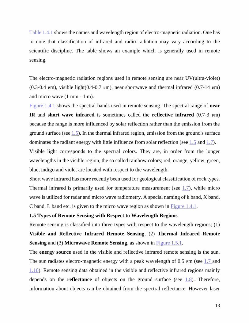
Figure 1.4.1 shows the spectral bands used in remote sensing. The spectral range of near

IR and short wave infrared is sometimes called the reflective infrared (0.7-3 m)

because the range is more influenced by solar reflection rather than the emission from the

ground surface (see 1.5). In the thermal infrared region, emission from the ground's surface

dominates the radiant energy with little influence from solar reflection (see 1.5 and 1.7).

Visible light corresponds to the spectral colors. They are, in order from the longer

wavelengths in the visible region, the so called rainbow colors; red, orange, yellow, green,

blue, indigo and violet are located with respect to the wavelength.

Short wave infrared has more recently been used for geological classification of rock types.

Thermal infrared is primarily used for temperature measurement (see 1.7), while micro

wave is utilized for radar and micro wave radiometry. A special naming of k band, X band,

C band, L band etc. is given to the micro wave region as shown in Figure 1.4.1.

1.5 Types of Remote Sensing with Respect to Wavelength Regions

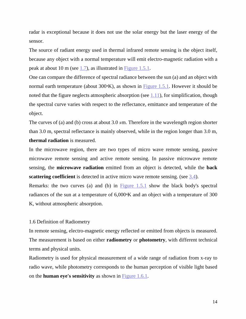
Remote sensing is classified into three types with respect to the wavelength regions; (1)

Visible and Reflective Infrared Remote Sensing, (2) Thermal Infrared Remote

Sensing and (3) Microwave Remote Sensing, as shown in Figure 1.5.1.

The energy source used in the visible and reflective infrared remote sensing is the sun.

The sun radiates electro-magnetic energy with a peak wavelength of 0.5 m (see 1.7 and

1.10). Remote sensing data obtained in the visible and reflective infrared regions mainly

depends on the reflectance of objects on the ground surface (see 1.8). Therefore,

information about objects can be obtained from the spectral reflectance. However laser

14

radar is exceptional because it does not use the solar energy but the laser energy of the

sensor.

The source of radiant energy used in thermal infrared remote sensing is the object itself,

because any object with a normal temperature will emit electro-magnetic radiation with a

peak at about 10 m (see 1.7), as illustrated in Figure 1.5.1.

One can compare the difference of spectral radiance between the sun (a) and an object with

normal earth temperature (about 300 K), as shown in Figure 1.5.1. However it should be

noted that the figure neglects atmospheric absorption (see 1.11), for simplification, though

the spectral curve varies with respect to the reflectance, emittance and temperature of the

object.

The curves of (a) and (b) cross at about 3.0 m. Therefore in the wavelength region shorter

than 3.0 m, spectral reflectance is mainly observed, while in the region longer than 3.0 m,

thermal radiation is measured.

In the microwave region, there are two types of micro wave remote sensing, passive

microwave remote sensing and active remote sensing. In passive microwave remote

sensing, the microwave radiation emitted from an object is detected, while the back

scattering coefficient is detected in active micro wave remote sensing. (see 3.4).

Remarks: the two curves (a) and (b) in Figure 1.5.1 show the black body's spectral

radiances of the sun at a temperature of 6,000 K and an object with a temperature of 300

K, without atmospheric absorption.

1.6 Definition of Radiometry

In remote sensing, electro-magnetic energy reflected or emitted from objects is measured.

The measurement is based on either radiometry or photometry, with different technical

terms and physical units.

Radiometry is used for physical measurement of a wide range of radiation from x-ray to

radio wave, while photometry corresponds to the human perception of visible light based

on the human eye's sensitivity as shown in Figure 1.6.1.

15

Figure 1.6.1shows the rdoiometric definitions of radiant energy, radiant fiux, radiant

intensity, irradiance, raiant emittance and radiance.

Table 1.6.1 show the comparision with respect to the techical terms, symbols and units

between radiometry and photometry.

One can add an adjective "Spectral" before the technical terms of radiometry when defined

as per unit of wavelength. For example, one can use spectral radiant flux ( W m ) or

spectral radiance (Wm sr m ).

Radiant energy is defined as the energy carried by electro- magnetic radiation and

expressed in the unit of joule (J).

Radiant flux is radiant energy transmitted as a radial direction per unit time and expressed

in a unit of watt (W). Radiant intensity is radiant flux radiated from a point source per

unit solid angle in a radiant direction and expressed in the unit of Wsr . Irradiance is

radiant flux incident upon a surface per unit area and expressed in the unit of Wm .

Radiant emittance is radiant flux radiated from a surface per unit area, and expressed in

a unit of Wm . Radiance is radiant intensity per unit projected area in a radial direction

and expressed in the unit of Wm sg .

1.7 Black Body Radiation

An object radiates unique spectral radiant flux depending on the temperature and emissivity

of the object. This radiation is called thermal radiation because it mainly depends on

temperature. Thermal radiation can be expressed in terms of black body theory.

A black body is matter which absorbs all electro-magnetic energy incident upon it and does

not reflect nor transmit any energy. According to Kirchhoff's law the ratio of the radiated

energy from an object in thermal static equilibrium, to the absorbed energy is constant and

only dependent on the wavelength and the temperature T. A black body shows the

maximum radiation as compared with other matter. Therefore a black body is called a

perfect radiator.

16

Black body radiation is defined as thermal radiation of a black body, and can be given by

Plank's law as a function of temperature T and wavelength as shown in Figure 1.7.1 and

Table 1.7.1.

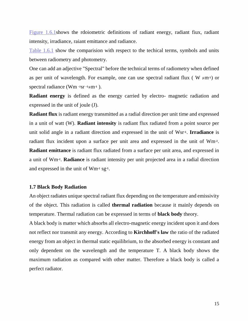
In remote sensing, a correction for emissivity should be made because normal observed

objects are not black bodies. Emissivity can be defined by the following formula-

Emissivity ranges between 0 and 1 depending on the dielectric constant of the object,

surface roughness, temperature, wavelength, look angle etc. Figure 1.7.2 shows the spectral

emissivity and spectral radiant flux for three objects that are a black body, a gray body

and a selective radiator.

The temperature of the black body which radiates the same radiant energy as an observed

object is called the brightness temperature of the object.

Stefan-Boltzmann's law is obtained by integrating the spectral radiance given by Plank's

law, and shows in that the radiant emittance is proportional to the fourth power of absolute

temperature (T ). This makes it very sensitive to temperature measurement and change.

Wien's displacement law is obtained by differentiating the spectral radiance, which shows

that the product of wavelength (corresponding to the maximum peak of spectral radiance)

and temperature, is approximately 3,000 ( m K). This law is useful for determining the

optimum wavelength for temperature measurement of objects with a temperature of T. For

example, about 10 m is the best for measurement of objects with a temperature of 300 K.

1.8 Reflectance

Reflectance is defined as the ratio of incident flux on a sample surface to reflected flux

from the surface as shown in Figure 1.8.1. Reflectance ranges from 0 to 1. Reflectance was

originally defined as a ratio of incident flux of white light to reflected flux in a hemisphere

direction. Equipment to measure reflectance are called spectrometers (see 2.6).

Albedo is defined as the reflectance using the incident light source from the sun.

Reflectance factor is sometime used as the ratio of reflected flux from a sample surface to

17

reflected flux from a perfectly diffuse surface. Reflectance with respect to wavelength is

called spectral reflectance as shown for a vegetation example in Figure 1.8.2. A basic

assumption in remote sensing is that spectral reflectance is unique and different from one

object to an unlike object.

Reflectance with a specified incident and reflected direction of electro-magnetic radiation

or light is called directional reflectance. The two directions of incident and reflection have

can be directional, conical or hemispherical making nine possible combinations.

For example, if incident and reflection are both directional, such reflectance is called

bidirectional reflectance as shown in Figure 1.8.3. The concept of bidirectional reflectance

is used in the design of sensors.

Remarks; A perfectly diffuse surface is defined as a uniformly diffuse surface with a

reflectance of 1, while the uniformly diffused surface, called a Lambertian surface, reflects

a constant radiance regardless of look angle.

The Lambert cosine law which defines a Lambertian surface is as follows:

I ( ) = In .cos

where I( ): luminous intensity at an angle of from the normal to the surface.

In : luminous intensity at the normal angle

1.9 Spectral Reflectance of Land Covers

Spectral reflectance is assumed to be different with respect to the type of land cover, as

explained in 1.3 and 1.8. This is the principle that in many cases allows the identification

of land covers with remote sensing by observing the spectral reflectance or spectral

radiance from a distance far removed from the surface.

Figure 1.9.1 shows three curves of spectral reflectance for typical land covers; vegetation,

soil and water. As seen in the figure, vegetation has a very high reflectance in the near

infrared region, though there are three low minima due to absorption.

Soil has rather higher values for almost all spectral regions. Water has almost no reflectance

in the infrared region.

18

Figure 1.9.2 shows two detailed curves of leaf reflectance and water absorption.

Chlorophyll, contained in a leaf, has strong absorption at 0.45 m and 0.67 m, and high

reflectance at near infrared (0.7-0.9 m). This results in a small peak at 0.5-0.6 (green color

band), which makes vegetation green to the human observer.

Near infrared is very useful for vegetation surveys and mapping because such a steep

gradient at 0.7-0.9 m is produced only by vegetation.

Because of the water content in a leaf, there are two absorption bands at about 1.5 m and

1.9 m. This is also used for surveying vegetation vigor.

Figure 1.9.3 shows a comparison of spectral reflectance among different species of

vegetation.

Figure 1.9.4 shows various patterns of spectral reflectance with respect to different rock

types in the short wave infrared (1.3-3.0 m). In order to classify such rock types with

different narrow bands of absorption, a multi-band sensor with a narrow wavelength

interval is to be developed. Imaging spectrometers (see 2.12) have been developed for rock

type classification and ocean color mapping.

1.10 Spectral Characteristics of Solar Radiation

The sun is the energy source used to detect reflective energy of ground surfaces in the

visible and near infrared regions.

Sunlight will be absorbed and scattered by ozone, dust, aerosols, etc., during the

transmission from outer space to the earths surface (see 1.11 and 1.12). Therefore, one has

to study the basic characteristics of solar radiation.

The sun is considered as a black body with a temperature of 5,900 K. If the annual average

of solar spectral irradiance is given by FeO( ), then the solar spectral irradiance Fe(l) in

outer space at Julian day D, is given by the following formula.

Fe( ) = FeO( ){1 + cos (2 (D-3)/365)}

where : 0.167 (eccentricity of the Earth orbit) : wavelength

D-3: shift due to January 3 as apogee and July 2 as perigee

The sun constant that is obtained by integrating the spectral irradiance for all wavelength

regions is normally taken as 1.37Wm . Figure 1.10.1 shows four observation records of

19

solar spectral irradiance. The values of the curves correspond to the value at the surface

perpendicular to the normal direction of the sun light. To convert to the spectral irradiance

per m on the Earth surface with a latitude of , multiply the following coefficient by the

observed values in Figure 1.10.1.

= (L0 / L) cos z cosz = sin sin + cos cos cos h

where z : solar zenith angle

: declination

h : hour angle,

L : real distance between the sun and the earth

L0: average distance between the sun and the earth

The incident solar radiation at the earth's surface is very different to that at the top of the

atmosphere due to atmospheric effects, as shown in Figure 1.10.2, which compares the

solar spectral irradiance at the earth's surface to black body irradiance from a surface of

temperature 5900 K.

The solar spectral irradiance at the earth's surface is influenced by the atmospheric

conditions and the zenith angle of the sun. Beside the direct sunlight falling on a surface,

there is another light source called sky radiation, diffuse radiation or skylight, which is

produced by the scattering of the sunlight by atmospheric molecules and aerosols.

The skylight is about 10 percent of the direct sunlight when the sky is clear and the sun's

elevation angle is about 50 degree. The skylight has a peak in its spectral characteristic

curve at a wavelength of 0.45 m

1.11 Transmittance of the Atmosphere

The sunlight's transmission through the atmosphere is affected by absorption and

scattering of atmospheric molecules and aerosols. The reduction of sunlight intensity is

called extinction. The rate of extinction is expressed as extinction coefficient (see 1.12).

20

The optical thickness of the atmosphere corresponds to the integrated value of the

extinction coefficient at each altitude by the atmospheric thickness. The optical thickness

indicates the magnitude of absorption and scattering of the sunlight. The following

elements will influence the transmittance of the atmosphere.

a. Atmospheric molecules(smaller size than wavelength):

carbon dioxygen, ozone, nitrogen gas, and other molecules

b. Aerosols (larger size than wavelength):

water drops such as fog and haze, smog, dust and other particles with a bigger size

Scattering by atmospheric molecules with a smaller size than the wavelength of the sunlight

is called Rayleigh scattering. Raleigh scattering is inversely proportional to the fourth

power of the wavelength.

The contribution of atmospheric molecules to the optical thickness is almost constant

spatially and with time, although it varies somewhat depending on the season and the

latitude.

Scattering by aerosols with larger size than the wavelength of the sunlight is called Mie

scattering. The source of aerosols will be suspended particles such as sea water or dust in

the atmosphere blown from the sea or the ground, urban garbage, industrial smoke,

volcanic ashes etc., which varies to a great extent depending upon the location and the time.

In addition, the optical characteristics and the size distribution also changes with respect to

humidity, temperature and other environmental conditions. This makes it difficult to

measure the effect of aerosol scattering.

Scattering, absorption and transmittance of the atmosphere are different for different

wavelengths. Figure 1.11.1 shows the spectral transmittance of the atmosphere. The low

parts of the curve show the effect of absorption by the molecules described in the figure.

Figure 1.11.2 shows the spectral transmittance, or conversely absorption, with respect to

various atmospheric molecules. The open region with higher transmittance in called "an

atmospheric window".

As the transmittance partially includes the effect of scattering, the contribution of scattering

is larger in the shorter wavelengths. Figure 1.11.3 shows a result of simulation for resultant

21

transmittance multiplied by absorption and scattering which would be produced for a

standard "clean atmospheric model" in the U.S.A. The contribution by scattering is

dominant in the region less than 2mm and proportional according to the shorter

wavelength. The contribution by absorption is not constant but depends on the specific

wavelength.

1.12 Radiative Transfer Equation

Radiative transfer is defined as the process of transmission of the electro-magnetic

radiation through the atmosphere, and the influence of the atmosphere. The atmospheric

effect is classified into multiplicative effects and additive effects as shown in Table 1.12.1.

The multiplicative effect comes from the extinction by which incident energy from the

earth to a sensor will reduce due to the influence of absorption and scattering. The additive

effect comes from the emission produced by thermal radiation from the atmosphere and

atmospheric scattering, which is incident energy on a sensor from sources other than the

object being measured.

Figure 1.12.1 shows a schematic model for the absorption of the electro-magnetic radiation

between an object and a sensor, while Figure 1.12.2 shows a schematic model for the

extinction. Absorption will occur at specific wavelengths (see 1.11) when the electro-

magnetic energy converts to thermal energy. On the other hand, scattering is remarkable in

the shorter wavelength region when energy conversion does not occur but only the

direction of the path changes.

As shown in Figures 1.12.3 and 1.12.4, additional energy by emission and scattering of the

atmosphere is incident upon a sensor. The thermal radiation of the atmosphere which is

characterized by Plank's law (see 1.7), is uniform in all directions. The emission and

scattering of the atmosphere incident on the sensor, is indirectly input from other energy

sources of scattering than those on the path between a sensor and an object.

The scattering depends on the size of particles and the direction of incident light and

scattering.

Thermal radiation is dominant in the thermal infrared region, while scattering is dominant

in the shorter wavelength region.

22

Generally, as extinction and emission occur at the same time,both effects should be

considered together in the radiative transfer equation as indicated in the formula in Table

1.12.2.

Chapter 2 Sensor

2.1 Types of Sensor

Figure 2.1.1 summarizes the types of sensors now used or being developed in remote

sensing. It is expected that some new types of sensors will be developed in the future.

23

Passive sensors detect the reflected or emitted electro-magnetic radiation from natural

sources, while active sensors detect reflected responses from objects which are irradiated

from artificially generated energy sources, such as radar.. Each is divided further in to non-

scanning and scanning systems.

A sensor classified as a combination of passive, non-scanning and non-imaging method

is a type of profile recorder, for example a microwave radiometer. A sensor classified as

passive, non-scanning and imaging method, is a camera, such as an aerial survey camera

or a space camera, for example on board the Russian COSMOS satellite.

Sensors classified as a combination of passive, scanning and imaging are classified further

into image plane scanning sensors, such as TV cameras and solid state scanners, and

object plane scanning sensors, such as multispectral scanners (optical-mechanical

scanner) and scanning microwave radiometers.

An example of an active, non-scanning and non-imaging sensor is a profile recorder such

as a laser spectrometer and laser altimeter. An active, scanning and imaging sensor is a

radar, for example synthetic aperture radar (SAR), which can produce high resolution,

imagery, day or night, even under cloud cover.

The most popular sensors used in remote sensing are the camera, solid state scanner, such

as the CCD (charge coupled device) images, the multi-spectral scanner and in the future

the passive synthetic aperture radar.

Laser sensors have recently begun to be used more frequently for monitoring air pollution

by laser spectrometers and for measurement of distance by laser altimeters.

Figure 2.1.2 shows the most common sensors and their spectral bands.

Those sensors which use lenses in the visible and reflective infrared region, are called

optical sensors

2.2 Characteristics of Optical Sensors Radiation

Optical sensors are characterized specified by spectral, radiometric and geometric

performance. Figure 2.2.1 summarizes the related elements for the three characteristics of

optical sensor. Table 2.2.1 presents the definitions of these elements.

24

The spectral characteristics are spectral band and band width, the central wavelength,

response sensitivity at the edges of band, spectral sensitivity at outer wavelengths and

sensitivity of polarization.

Sensors using film are characterized by the sensitivity of film and the transmittance of the

filter, and nature of the lens. Scanner type sensors are specified by the spectral

characteristics of the detector and the spectral splitter. In addition, chromatic aberration is

an influential factor. The radiometric characteristics of optical sensors are specified by

the change of electro-magnetic radiation which passes through an optical system. They are

radiometry of the sensor, sensitivity in noise equivalent power, dynamic range, signal to

noise ratio (S/N ratio) and other noises, including quantification noise.

The geometric characteristics are specified by those geometric factors such as field of view

(FOV), instantaneous field of news (IFOV), band to band registration, MTF (see 2.3),

geometric distortion and alignment of optical elements.

IFOV is defined as the angle contained by the minimum area that can be detected by a

scanner type sensor. For example in the case of an IFOV of 2.5 milli radians, the detected

area on the ground will be 2.5 meters x 2.5 meters,if the altitude of sensor is 1,000 m above

ground.

2.3 Resolving Power Radiation

Resolving power is an index used to represent the limit of spatial observation. In optics,

the minimum detectable distance between two image points is called resolving limit, and

the reverse is defined as the resolving power.

There are several methods to measure the resolving limit or resolving power. Two such

methods, (1) resolving power by refraction and (2) MTF, are introduced below.

(1) Resolving limit by refraction

Theoretically an object point will be projected as a point on an image plane if the optical

system has no aberration. However, because of diffraction the image of a point will be

a circle with a radius of about one wavelength of light, which in called the Airy

pattern, as shown in Figure 2.3.1. Therefore there exists a limit to resolve the distance

between two points even though there is no aberration.

25

The resolving limit depends on how the minimum distance between two Airy images is

defined. There are two definitions, as follows.

a. Rayleigh's resolving power: the distance between the left Airy peak and the right Airy

peak when it coincides with the zero point of the left peak, that is 1.22u in Figure 2.3.2.

b. Sparrow's resolving limit: the distance between the two peaks when the central gap

fades away, that is 1.08u in Figure 2.3.3 .

(2) MTF (modular transfer function )

The resolving power measured on a resolving test chart by human eyes, depends on

individual ability and the shape or contrast of the chart. On the other hand, MTF has no

such problems because MTF comes from a scientific definition in which the response of

spatial frequency, with respect to the amplitude, considers the optical imaging system as a

spatial frequency filter.

As the spatial frequency is defined as the frequency of a sine wave, MTF shows how much

the ratio of the amplitude decreases before and after an optical imaging system with respect

to the spatial frequency as shown in Figure 2.3.4.

MTF coincides with the power spectrum which is obtained by Fourier transformation of a

point image. Generally speaking, an optical imaging system will give a low pass filter as

shown in Figure 2.3.5.

Modulation (M), contrast (K) and density (D) have the following relations.

= max / min, D = log( max / min), M = ( max - min ) / ( max + min ) = ( - 1) / (

+ 1)

' = 'max / 'min, D' = log( 'max / min), M = ( 'max - 'min ) / ( 'max + 'min ) = ( ' -

1) / ( ' + 1)

The resolving power (or spatial frequency) is obtained from the MTF curve with a given

contrast, which can be converted to the modulation.

2.4 Dispersing Element

An array of light arranged by order of wavelength is called a spectrum. Spectroscopy is

defined as the study of the dispersion of light into its spectrum. There are two types of

dispersing elements, the prism and the diffraction grating.

26

Figure 2.4.1 shows the types of dispersing elements. The optical mechanism of prisms and

diffraction gratings are shown in Figure 2.4.2 and Figure 2.4.3 respectively.

(1) Prism

A prism designed for spectroscopy is called a dispersing prism, which is based on the

theory that refractive index is different depending on the wavelength, as shown in Figure

2.4.4. The spectral resolution of a prism is much lower than that of a diffraction grating. If

higher spectral resolution is required, a layer prism should be produced. This can be a

problem, because it is rather difficult to prepare homogeneous material and to keep the

weight low.

(2) Diffraction grating

A diffraction grating is a diffraction element which utilizes the theory that incident light to

a grating is dispersed in multiple different directions depending on the difference of light

path length or phase difference between two neighboring gratings. Multiple spectra are

generated in integer order direction in which multiplication by the wavelength corresponds

to the light path difference as shown in Figure 2.4.5. Most diffraction gratings are reflection

type rather than transparency type. Though the specular diffraction gives the maximum

intensity as 0 order diffraction, it cannot be utilized because 0 order diffraction does not

produce a spectrum. Therefore a reflecting plane is adjusted to have a proper angle to obtain

a strong enough spectrum at a certain order. Such an adjusted grating is called a blazed

grating.

2.5 Spectroscopic Filter

A filter can transmit or reflect a specified range of wavelength. A filter designed for

spectroscopy is called a spectroscopic filter.

Filters are classified into three types - long wave pass filters, short wave pass filters and

band pass filters from the viewpoint of function, as shown in Figure 2.5.1. A cold mirror

which transmits thermal infrared and reflects visible light is a long wave pass filter, while

a hot mirror which reflects thermal infrared and transmits visible light is a short wave filter.

Figure 2.5.2 shows the types of filter from the viewpoint of function.

(1) Absorption filter :

27

a filter which absorbs a specific range of wavelengths, for examples, colored filter

glass and gelatin filter.

(2) Interference filter :

a filter which transmits a specific range of wavelengths by utilizing the interference effect

of a thin film. When light is incident on a thin film, only a specific range of wavelengths

will pass due to the interference by multiple reflection in a thin film as shown in Figure

2.5.3 and 2.5.4. The higher the reflectance of the thin film, the narrower the width of the

spectral band becomes. If two of these films, with different refractive indexes, are

combined, the reflectance becomes very high which results in a narrow spectral band, for

example of the order of several nanometers. In order to obtain a band pass filter which

transmits a single spectral band, a short wave pass filter and long wave pass filter should

be combined. A dichroic mirror ,which is used for three primary color separation, is a kind

of multiple layer interference filter, as shown in Figure 2.5.5 and 2.5.6. It utilizes both

functions of transparency and reflection.

(3) Diffraction grating filter :

a reflective long wave pass filter utilizing the diffraction effect of a grating, which reflects

all light of wavelengths longer than the wavelength determined by the grating interval and

the oblique angle of the incident radiation.

(4) Polarizing interference filter :

a filter with birefringent crystallinity plate between two polarizing plates, which pass a very

narrow spectral band, for example less than 0.1 mm. This utilizes the interference by two

rays of light ; a light following Snell's law and the other not following Snell's law, which

pass a light with a narrow band of wavelength determined by the thickness of the

birefringent crystallinity plate .

2.6 Spectrometer

There are many kinds of spectral measurement devices ,for example, spectroscopes for

human eye observation of the spectrum, spectrometer to record spectral reflectance,

monochro meter to read a single narrow band, spectro photometer for photometry,

28

spectro radiometer for measurement of spectral radiation etc. However, in this section

only optical spectrometers are of interest.

Figure 2.6.1 shows a classification of spectrometers, which are divided mainly into

dispersing spectrometers and interference spectrometers. The former utilizes prisms or

diffraction gratings, while the latter the interference of light. (1) Dispersing spectrometer

A spectrum is obtained at the focal plane after a light ray passes through a slit and

dispersing element as shown in Figure 2.6.2. Figure 2.6.3 and Figure 2.6.4 are typical

dispersing spectrometers ; Littnow spectrometer and Czerny - Turner spectrometer

respectively.

(2) Twin beam interference spectrometer

A distribution of the spectrum is obtained by cosine Fourier transformation of the

interferogram which is produced by the inference between two split rays. Figure 2.6.5

shows Michelson interferometer which utilizes a beam splitter.

(3) Multi-beam interference spectrometer

The interference of light will occur if oblique light is incident on two parallel semi-

transparent plane mirrors. A different spectrum is obtained depending on incident angle,

interval of the two mirrors and the refraction coefficient.

2.7 Characteristics of Optical Detectors

An element which converts the electro-magnetic energy to an electric signal is called a

detector. There are various types of detectors with respect to the detecting wavelength.

Figure 2.7.1 shows three types of detectors; photo emission type, optical excitation type

and thermal effect type. Photo tube and photo multiplier tubes are the examples of the

photo emission type which has sensitivity in the region from ultra violet to visible light.

Figure 2.7.2 shows the response sensitivity of several photo tubes.

Photodiode, phototransistor, photo conductive detectors and linear array sensors (see

2.11), are examples of optical excitation types, which have sensitivity in the infrared

region. Photo diode detectors utilize electric voltage from the excitation of electrons, while

photo transistor and photo conductive detector utilize electric current. Table 2.7.1 shows

29

the characteristics of these optical detectors with respect to type, temperature, range of

wavelength, peak wavelength, sensitivity in term of D* and response time.

Thermocouple barometers and pyroelectric barometers are examples of the thermal

effect type, which has sensitivity from near infrared to far infrared regions. However the

response is not very high because of the thermal effect. Figure 2.7.3 shows the detectivity

of the pyroelectric barometer.

Detectivity denoted as D* (termed D star) is usually related to the sensitivity, expressed as

NEP (noise equivalent power). D* is used for comparison between different detectors.

NEP is defined as the signal input identical to the noise output. NEP depends on the type

of detector, surface of detector or band of frequency. D* is inversely proportional to NEP,

and is given as follows.

D* : (Ad f ) / NEP

D* : detectivity (cm Hz / W)

NEP : noise equivalent power (W)

Ad : surface area of detector ( cm )

f : band of frequency ( Hz )

2.8 Cameras for Remote Sensing

Aerial survey cameras, multispectral cameras, panoramic cameras etc. are used for

remote sensing.

Aerial survey cameras, sometimes called metric cameras are usually used on board aircraft

or space craft for topographic mapping by taking stereo photographs with overlap. A

typical aerial survey camera is RMK made by Carl Zeiss or RC series made by Leica

company. Figure 2.8.1 shows the mechanics of the Zeiss RMK aerial survey camera.

Typical well known, examples of space cameras, are the Metric Camera on board the

Space Shuttle by ESA, the Large Format Camera also on board the Space Shuttle by

NASA, and the KFA 1000 on board COSMOS by Russia. Figure 2.8.2 shows the LFC

system and its film size. Figure 2.8.3 shows a comparison of photographic coverage on the

ground between LFC (173 km x 173 km) and KFA (75 km x 75 km).

30

As the metric camera is designed for very accurate measurement of topography, the

following requirements in optics as well as geometry should be specified and fulfilled.

(1) Lens distortion should be minimal

(2) Lens resolution should be high and the image should be very sharp even in the corners

(3) Geometric relation between the frame and the optical axis should be established, which

is usually achieved by fiducial marks or reseau marks

(4) Lens axes and film plane should be vertical to each other.

(5) Film flatness should be maintained by a vacuum pressure plate

(6) Focal length should be measured and calibrated accurately

(7) Successive photographs should be mode with high speed shutter and film winding

system

(8) Forward Motion Compensation (FMC) to prevent the image motion of high speed

moving objects during shutter time, should be used, particularly in the case of space

cameras

Multispectral cameras with several separate film scenes in the visible and reflective IR, are

mainly used for photo-interpretation of land surface covers.

Figure 2.8.4 shows a picture taken by the MKF-4, with 4 bands, on board the Russian

Soyuz 22.

Panoramic cameras are used for reconnaissance surveys, surveillance of electric

transmission lines, supplementary photography with thermal imagery, etc., because the

field of view is so wide.

2.9 Film for Remote Sensing

Various type of films are used in cameras for remote sensing. Film can record the

electromagnetic energy reflected from objects in the form of optical density in an emulsion

placed on a film base of polyester. There are panchromatic (black and white film),

infrared film, color film, color infrared film, etc.

The spectral sensitivity of film is different depending on the film type. Black and white

infrared film has wider sensitivity up to near infrared as compared with panchromatic film.

31

Color film has three different spectral sensitivities according to three layers of primary

color emulsion (B,G, R). Color infrared film has sensitivity up to 900 nm. Kodak aerial

color film SO-242 has high resolution and is specially ordered for high altitude

photography.

Generally film is composed of a photographic emulsion which records various gray levels

from white to black according to the reflectivity of objects.

A curve which shows the relationship between the exposure E (meter caudera second) and

the photographic density is called the "characteristic curve". Usually the horizontal axis

of the curve is log E, while the vertical axis is D (density) which is given as follow.

D = log (1 / T ) where T : transparency of film

The characteristic curve is composed of three parts of toe, straight line and shoulder.

Gamma is defined as the gradient of the straight line part, which is an index of contrast. If

is given by D / logE which gives high contrast in the case of gamma larger than 1.0,

and low contrast in the case of gamma smaller than 1.0.

The sensitivity of a photographic emulsion is defined as the minimum exposure to give the

minimum recognizable density. In the definition of JIS (Japan Industrial Standard), the

sensitivity is given as log (1 / EA ) under the conditions of exposure and development

density as denoted ( EA, EB ) and ( A, B ) respectively,

where A : the gross fog + 0.1 EB : EA + 1.5 0.75 < B - A < 0.9

The spectral sensitivity of photographic emulsion (S ) represents the sensitivity with

respect to each wavelength, which is usually given in the form of a spectral sensitivity

curve. In the spectral sensitivity curve log S is used instead of S as the vertical axis, while

sometimes relative sensitivity is used.

Figure 2.9.3 (a) - (d) show the spectral sensitivity curves corresponding to panchromatic,

infrared,color and color infrared films respectively.

2.10 Optical Mechanical Scanner

An optical mechanical scanner is a multispectral radiometer by which two dimensional

imagery can be recorded using a combination of the motion of the platform and a rotating

or oscillating mirror scanning perpendicular to the flight direction. Optical mechanical

32

scanners are composed of an optical system, spectrographic system, scanning system,

detector system and reference system.

Optical mechanical scanners can be carried on polar orbit satellites or aircraft.

Multispectral scanner (MSS) and thematic mapper (TM) of LANDSAT, and Advanced

Very High Resolution Radiometer (AVHRR) of NOAA are the examples of optical

mechanical scanners. M2S made by Daedalus Company is an example of an airborne type

optical mechanical scanner.

Figure 2.10.1 shows the concept of optical mechanical scanners, while Figure 2.10.2 shows

a schematic diagram of the optical process of an optical mechanical scanner.

The function of the elements of an optical mechanical scanner are as follows.

a. Optical system: Reflective telescope system such as Newton, Cassegrain or Ritchey-

Chretien is used to avoid color aberration.

b. Spectrographic system: Dichroic mirror, grating, prism or filter are utilized.

c. Scanning system: rotating mirror or oscillating mirror is used for scanning perpendicular

to the flight direction.

d. Detector system: Electro magnetic energy is converted to an electric signal by the optical

electronic detectors. Photomultiplier detectors utilized in the near ultra violet and visible

region, silicon diode in the visible and near infrared, cooled ingium antimony (InSb) in the

short wave infrared, and thermal barometer or cooled Hq Cd Te in the thermal infrared.

e. Reference system: The converted electric signal is influenced by a change of sensitivity

of the detector. Therefore light sources or thermal sources with constant intensity or

temperature should be installed as a reference for calibration of the electric signal.

Compared to the pushbroom scanner, the optical mechanical scanner has certain

advantages. For examples, the view angle of the optical system can be very narrow, band

to band registration error is small and resolution is higher, while it has the disadvantage

that signal to noise ratio (S/N) is rather less because the integration time at the optical

detector cannot be very long due to the scanner motion.

2.11 Pushbroom Scanner

33

The pushbroom scanner or linear array sensor is a scanner without any mechanical

scanning mirror but with a linear array of solid semiconductive elements which enables

it to record one line of an image simultaneously, as shown is Figure 2.11.1.

The pushbroom scanner has an optical lens through which a line image is detected

simultaneously perpendicular to the flight direction. Though the optical mechanical

scanner scans and records mechanically pixel by pixel, the pushbroom scanner scans and

records electronically line by line.

Figure 2.11.2 shows an example of the electronic scanning scheme by switching method.

Because pushbroom scanners have no mechanical parts, their mechanical reliability can be

very high.

However, there will be some line noise because of sensitivity differences between the

detecting elements.

Charge coupled devices, called CCD, are mostly adopted for linear array sensors.

Therefore it is sometime called a linear CCD sensor or CCD camera. HRV of SPOT,

MESSR of MOS-1, and OPS of JERS-1 are examples of linear CCD sensors as is the Itres

CASI airborne system. As an example, MESSR of MOS-1 has 2048 elements with an

interval of 14 mm. However CCD with 5,000 - 10,000 detector elements have been

developed and available recently made available.

2.12 Imaging Spectrometer

Imaging spectrometers are characterized by a multispectral scanner with a very large

number of channels (64-256 channels) with very narrow band widths, though the basic

scheme is almost the same as an optical mechanical scanner or pushbroom scanner.

The optical system of imaging spectrometers are classified into three types; dioptic system,

dio and catoptic system and catoptic system which are adopted depending on the scanning

system. Table 2.12.1 shows a comparison of the three types. In the case of object plane

scanning, the catoptic system is best chosen because the linearity of the optical axis is very

good due to the narrow view angle and the observation wave range is so wide. However in

34

the case of image plane scanning, the dioptic system or dioptic and catoptic system is best

suited because the view angle should be wider.

Figure 2.12.1 shows four different types of multispectral scanner. The left upper

(multispectral imaging with discrete detectors) corresponds to the optical mechanical

scanner on the using the object plane scanning method used in the LANDSAT. The right

upper (multispectral imaging with line arrays) corresponds to pushbroom scanner using the

image plane scanning method with a linear CCD array.

The left lower (imaging spectrometry with line arrays) shows a similar scheme to the right

upper system but with an additional dispersing element (grating or prism) to increase the

spectral resolution. The right lower (imaging spectrometry with area arrays) shows an

imaging spectrometer with area arrays.

Table 2.12.2 shows the optical scheme of the Moderate Resolution Imaging Spectrometer-

Tilt (MODIS-T) which is scheduled to be carried on EOS-a (US Earth Observing

Satellite). MODIS-T has an area array of 64 x 64 elements which enables 64 multispectral

bands from 0.4 mm to 1.04 mm with a 64 km swath. The optical path is guided from scan

mirror to Schmitt type off axis parabola of dio and catoptic system. The the light is then

dispersed into 64 bands by a grating and is detected by an area CCD array of 64 x 64

elements.

As imaging spectrometer provides multiband imagery with a narrow wave length range,

and is useful for rock type classification and ocean color analysis.

2.13 Atmospheric Sensors

Atmospheric sensors are designed to provide measures of air temperature, vapor,

atmospheric constituents, aerosols the etc. as well as wind and earth radiation budget.

Figure 2.13.1 shows the important atmospheric constituents for green house effect gases,

ozone layer and acid rain.

As remote sensing techniques cannot meet the direct measurement of these physical

magnitude, it is necessary to estimate them from spectral measurement of atmospheric

scattering, absorptance or emission.

35

The spectral wave length range is very wide from the near ultraviolet to the millimeter

radio wave depending on the objects to be measured (See 1.4).

There are two types of atmospheric sensor, that is, active and passive . Because the active

sensor is explained in section 2.15 "Laser Radar" or Lidar,only the passive type sensors

will be introduced here.

Two directions of atmospheric observation are usually adopted; one is nadir observation

and the other is limb observation as shown in Figure 2.13.1. The nadir observation is

superior in the horizontal resolution compared to vertical resolution. It is mainly useful in

the troposphere but not in the stratosphere where the atmospheric density is very low.

The limb observation method is to measure the limb of the earth with an oblique angle.

In this case, not only atmospheric emission but also atmospheric absorption of the light of

the sun, the moon and the stars are measured, as shown in Figure 2.13.1. Compared with

the nadir observation, the limb observation has higher vertical resolution and higher

measurability in the stratosphere. The absorption type of limb observation has rather high

S/N but observation direction or area is limited except for the stars.

There are two types of atmospheric sensors, that is, sensors with a fixed observation

direction, called sounders and scanners.

The main element of optical sensor is a spectrometer with a very high spectral resolution

such as the Michelson spectrometer, Fabry-Perot spectrometer and other spectrometers

with grating and prism.

Figure 2.13.2 shows the structure of Michelson spectrometer called IMG which will be

borne on ADEOS (Advanced Earth Observing Satellite to be launched in 1995 by Japan).

2.14 Sonar

Sound waves or ultrasonic waves are used underwater to obtain imagery of geological

features at the bottom of the sea or lakes because radio waves are not usable in water.

Sound waves have many characteristics such as reflection, refraction, interference,

diffraction etc. similar to radio waves, though it is an elastic wave different from the radio

wave. Sound waves have a form of longitudinal wave in water along the direction of the

wave. Generally, sound waves transmitting in water have a higher resolution according to

36

higher frequency but also higher attenuation. The detectability depends on S/N ratio when

receiving the sound signal after loss by noises in water.

The velocity of sound is approximately 1,500 meters/second which varies depending on

temperature, water pressure, and salinity of the medium.

As shown in Figure 2.14.1, there are side scan sonar and multi-beam echo sounder by

which the sea bottom is scanned and imaged. These sensors are kinds of active sensors

which record the sound intensity reflected from the projected sound wave onto the bottom.

Because sonar is an active sensor, it generates image distortion from the effects of

foreshortening, layover and shadow, with respect to incident angle at the bottom, in the

same manners as radar.

As shown in Figure 2.14.2, a side scan wave is produced from a transducer borne on a

towfish connected by tow cable to a tug boat. The incident sound wave on the sea bottom

will produce sound pressure on the bottom materials causing back scattering to return to

the receiver, after attenuation, according to the shape and density of the bottom. The sonar

acquires the backscattering in the time sequence to a form of image.

Figure 2.14.3 shows a multi narrow beam sounder with a transmitting transducer and a

receiving transducer in a T shape at the bottom of the boat. A receiving transduce has 20

to 60 elements which receive the sound signal reflected from the sea bottom, which is

usually converted to an image as for the side scan sonar.

2.15 Laser Radar

Devices which measures the physical characteristics such as distance, density, velocity,

shape etc., using scattering, returned time, intensity, frequency and/or polarization of light

are called optical sensors. However as the actual light used by the optical sensor is mostly

laser, it is usually called laser radar or lidar (light detection and ranging).

Laser radar is an active sensor which is used to measure air pollution, physical

characteristics of atmospheric constituents in the stratosphere and its spatial distribution.

The theory of laser radar is also utilized to measure distance, so that for this application it

is called laser distancemeter or laser altimeter.

37

The main measurement object is the atmosphere although laser radar is also used to

measure water depth, thickness of oil film or vividness of chlorophyll in vegetation.

[ Theory of Lidar ]

Figure 2.15.1 shows a schematic diagram of a lidar system. The power of the received light

Pr (R) reflected from a distance of R can be expressed as follows.

Pr (R) = Po K Ar q (R) T (R) Y (R) / R + Pb

where Po : intensity of transmitted light

K : efficiency of optical system

Ar : aperture

q : half wavelength

b (R) : backscattering coefficient

T (R) : transmittance of atmosphere

Y (R) : geometric efficiency

Pb : light noises of background

Received light is converted to an electric signal which is displayed or recorded after A/D

conversion. The effective distance of lidar depends on the relationship between the

received light intensity and the noise level.

Lidar can be classified with respect to its physical characteristics, interactive effects,

physical quantities etc., as shown in Table 2.15.1. In this table, Mie Lidar is the most

established sensor,with a which signal intensity large enough to measure Mie scattering

due to aerosols.

Fluorescence lidar, Roman lidar and differential absorption lidar Figure 2.15.3 are utilized

for measurement of density of gaseous body, while Doppler lidar is used for measurement

of velocity. Polarization effects of lidar is utilized for measurement of shape.

There are several display modes for example, a scope with horizontal axis of distance and

with vertical axis of intensity, PPI (plane position indication ) with gray level in polar

coordinate system, RHI (range high indication) with a display of the vertical profile, THI

(time height indication) with a horizontal axis of elapsed time and with a vertical axis of

altitude.

38

Chapter 3 Microwave Remote

Sensing

3.1 Principles of Microwave Remote Sensing

Microwave remote sensing, using microwave radiation using wavelengths from about one

centimeter to a few tens of centimeters enables observation in all weather conditions

without any restriction by cloud or rain. This is an advantage that is not possible with the

visible and/or infrared remote sensing. In addition, microwave remote sensing provides

39

unique information on for example, sea wind and wave direction, which are derived from

frequency characteristics, Doppler effect, polarization, back scattering etc. that cannot be

observed by visible and infrared sensors. However, the need for sophisticated data analysis

is the disadvantage in using microwave remote sensing.

There are two types of microwave remote sensing; active and passive. The active type

receives the backscattering which is reflected from the transmitted microwave which is

incident on the ground surface.

Synthetic aperture radar (SAR), microwave scatterometers, radar altimeters etc. are active

microwave sensors. The passive type receives the microwave radiation emitted from

objects on the ground. The microwave radiometer is one of the passive microwave sensors.

The process used by the active type, from the transmission by an antenna, to the reception

by the antenna is theoretically explained by the radar equation as described in Figure

3.1.1.

The process of the passive type is explained using the theory of radiative transfer based on

the law of Rayleigh Jeans as explained in Figure 3.1.2 (see 1.7, 1.12 and 3.2) In both active

and passive types, the sensor may be designed considering the optimum frequency needed

for the objects to be observed. (see 4.1)

In active microwave remote sensing, the characteristics of scattering can be derived from

the radar cross section calculated from received power Pr and antenna parameters (At ,

Pt , Gt ) and the relationship between them, and the physical characteristics of an object.

For example, rainfall can be measured from the relationship between the size of water drops

and the intensity of rainfall.

In passive microwave remote sensing, the characteristics of an object can be detected from

the relationship between the received power and the physical characteristics of the object

such as attenuation and/or radiation characteristics. (see 3.2 and 3.3)

3.2 Attenuation of Microwave

Attenuation results from absorption by atmospheric molecules or scattering by aerosols

in the atmosphere between the microwave sensor on board a spacecraft or aircraft and the

target to be measured. The attenuation of the microwave will take place as a function of

40

the exponential with respect to the transmitted distance mainly due to absorption and

scattering. Therefore the attenuation will increase in proportion to the distance, under

homogeneous atmospheric conditions. The attenuation per unit of distance is called

specific attenuation. Usually the loss due to attenuation can be expressed in the units of

dB (decibel) as follows.

dB = K e B dr

where Ke: specific attenuation (dBkm )

B : brightness temperative ( Wm sr ) in the distance of dr

dr : incremental distance

Figure 3.2.1 shows the attenuation characteristics of atmospheric molecules with respect

to frequency. From this figure it can be seen that the influence of atmospheric attenuation

occurs in the region greater than 10GHz. The intensity of attenuation depends on the

specific frequency (absorption spectrum) of the corresponding molecule. This is the reason

why the energy of the microwave is absorbed by the molecular motion of the atmospheric

constituent. However, if proper frequencies are carefully selected, the attenuation can be

minimized because the composition of the atmospheric constituent is almost homogeneous.

In the case of satellite observation, the optical path is usually long in distance, so that

attenuation can be influenced by the change in atmospheric conditions. Particularly

because the attenuation of vapor (H2O) is very strong in the specific frequencies, the

change of vapor can be detected by a microwave radiometer.

The most remarkable scattering in the atmosphere is due to rain drops. Figure 3.2.2 shows

the attenuation characteristics due to scattering of rain drops and mist. The attenuation

increases if the intensity of rainfall increases, and the frequency increases until about 40

GHz. However, over 40 GHz the attenuation does not depend on the frequency.

Remarks 1) dB is 1 / 10 bel.

"bel" is logarithmic ratio of two powers P1 and P2 .

N = log10 ( P1 / P2 ) [bel] or

n = 10 log10 ( P1 / P2 ) [dB]

41

2) Specific attenuation Ke is originally expressed as Np m or neepers m . But K e is

converted to dB km for convenience by multiplying 10 log e = 4.34 x 10 by Np m .

3.3 Microwave Radiation

The earth surface radiates a little microwave energy as well as visible and infrared because

of thermal radiation. The thermal radiation of a black body depends on Plank's law in the

visible and infrared region, while the thermal radiation in the microwave region is given

by the Rayleigh Jeans radiation law .

Real objects, the so called gray bodies are not identical to a black body but have constant

emissivity which is less than a blackbody . The brightness temperature TB is expressed

as follows.

TB = T

where T : physical temperature

: emissivity (0 < < 1)

Emissivity of an object changes depending on the permittivity, surface roughness,

frequency, polarization, incident angle, azimuth etc., which influence the brightness

temperature.

Figure 3.3.1 shows the characteristics of emissivity for 3.5 % density salt water with respect

to incident angle, polarization and frequency. Figure 3.3.2 shows the emissivity of

horizontal polarization (eh) and vertical polarization (ev) for two clay soils with different

soil moisture, and a sea water with respect to incident angle.

Table 3.3.1 shows the emissivity of typical land surface covers for two different grazing

angles of 30 and 45 .

Most users would like to get the physical temperature T instead of brightness temperature

TB , which is measured by microwave radiometers.

Therefore emissivity should be measured or algorithms should be developed to identify the

component of atmospheric radiation.

In the case of the receiving antenna of the microwave radiometer, all radiation from various

angles are input to the antenna, which needs a correction of the received temperature with

42

respect to directional properties of the antenna. The corrected temperature is called the

antenna temperature.

3.4 Surface Scattering

Surface scattering is defined as the scattering which takes place only on the border surface

between two different but homogeneous media, from one of which electro-magnetic energy

is incident on to the other. Scattering of microwave on the ground surface increases

according to the increase of complex permittivity, and the direction of scattering depends

on the surface roughness, as shown in Figure 3.4.1.

In the case of a smooth surface as shown in Figure 3.4.1 (a), there will be a specular

reflection with a symmetric angle to the incident angle. The intensity of specular

reflection is given by Fresnel reflectivity, which increases in accordance with the increase

of the ratio of complex permittivity.

When the surface roughness increases a little as shown in Figure 3.4.1 (b), there exists a

component of specular reflection and a scattering component. The component of specular

reflection is called the coherent component, while that of scattering is called diffuse or the

incoherent component.

When the surface is completely rough, that is diffuse, only diffuse components will remain

without any component of specular reflection as shown in Figure 3.4.1 (c). Such surface

scattering depends on the relationship between the wavelength of electro-magnetic

radiation and the surface roughness which is defined by the Rayleigh Criterion or

Fraunhofer Criterion.

Rayleigh Criterion : if h < / 8 cos , the surface is smooth

Fraunhofer Criterion : if h < / 32 cos , then the surface is smooth

where h : standard deviation of surface roughness

: wavelength

: incident angle

Generally the scattering coefficient, that is scattering area per unit area, is a function of

incident angle and the scattering angle. However in the case of remote sensing, the

scattering angle is identical to the incident angle because the receiving antenna of radar or

43

scatterometer is located at the same place as the transmitting antenna. Therefore, in remote

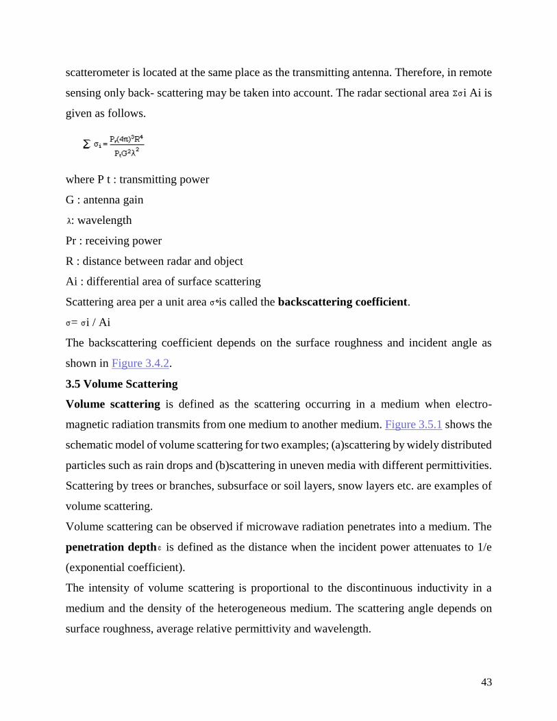
sensing only back- scattering may be taken into account. The radar sectional area i Ai is

given as follows.

where P t : transmitting power

G : antenna gain

: wavelength

Pr : receiving power

R : distance between radar and object

Ai : differential area of surface scattering

Scattering area per a unit area is called the backscattering coefficient.

= i / Ai

The backscattering coefficient depends on the surface roughness and incident angle as

shown in Figure 3.4.2.

3.5 Volume Scattering

Volume scattering is defined as the scattering occurring in a medium when electro-

magnetic radiation transmits from one medium to another medium. Figure 3.5.1 shows the

schematic model of volume scattering for two examples; (a)scattering by widely distributed

particles such as rain drops and (b)scattering in uneven media with different permittivities.

Scattering by trees or branches, subsurface or soil layers, snow layers etc. are examples of

volume scattering.

Volume scattering can be observed if microwave radiation penetrates into a medium. The

penetration depth is defined as the distance when the incident power attenuates to 1/e

(exponential coefficient).

The intensity of volume scattering is proportional to the discontinuous inductivity in a

medium and the density of the heterogeneous medium. The scattering angle depends on

surface roughness, average relative permittivity and wavelength.

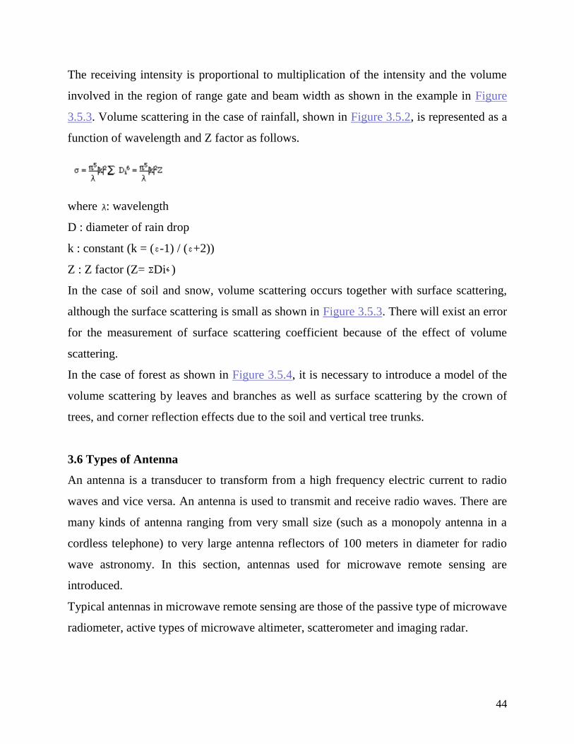
44

The receiving intensity is proportional to multiplication of the intensity and the volume

involved in the region of range gate and beam width as shown in the example in Figure

3.5.3. Volume scattering in the case of rainfall, shown in Figure 3.5.2, is represented as a

function of wavelength and Z factor as follows.

where : wavelength

D : diameter of rain drop

k : constant (k = ( -1) / ( +2))

Z : Z factor (Z= Di )

In the case of soil and snow, volume scattering occurs together with surface scattering,

although the surface scattering is small as shown in Figure 3.5.3. There will exist an error

for the measurement of surface scattering coefficient because of the effect of volume

scattering.

In the case of forest as shown in Figure 3.5.4, it is necessary to introduce a model of the

volume scattering by leaves and branches as well as surface scattering by the crown of

trees, and corner reflection effects due to the soil and vertical tree trunks.

3.6 Types of Antenna

An antenna is a transducer to transform from a high frequency electric current to radio

waves and vice versa. An antenna is used to transmit and receive radio waves. There are

many kinds of antenna ranging from very small size (such as a monopoly antenna in a

cordless telephone) to very large antenna reflectors of 100 meters in diameter for radio

wave astronomy. In this section, antennas used for microwave remote sensing are

introduced.

Typical antennas in microwave remote sensing are those of the passive type of microwave

radiometer, active types of microwave altimeter, scatterometer and imaging radar.

45

There are three major types of antenna; horn antenna, reflector mirror antenna and array

antenna.

The horn antenna such as the conical horn or rectangular horn is used for power supply to

the reflector antenna, calibration of low temperatures for the microwave radiometer in the

form of a sky horn looking upward, and calibration for active radar as shown in Figure

3.6.1.

Reflector antenna such as parabolic antenna and Cassegrainian antenna are composed of

primary radiator and a reflective mirror as shown in Figure 3.6.2. The reflector antenna is

used for microwave radiometers, altimeters and scatterometers. In case of wide angle

scanning, all antenna will be controlled, while in the case of narrow beam scanning only

the radiometer or reflective mirror will be controlled.

An array antenna is composed of multiple element arrays for example, linear array, area

array or nonformal array. The element antennas are half-wavelength dipoles, microstrip

patches and wave guide slot. The advantages of array antenna are to enable beam scanning

without changing the looking angle of each array antenna and to generate an appropriate

beam shaping by selective excitation of current distribution of each element.

The array antenna is used for synthetic aperture radar (SAR) and real aperture radar. Figure

3.6.3 shows a wave guide slot array antenna designed for real aperture radar.

3.7 Characteristics of Antenna

An ordinal antenna is used for transmitting radio waves in a specific direction or for

receiving radio waves from a specific direction. Therefore it can be said that the antenna is

a spatial filter for radio wave.

Relative power, given as a function of the beam angle is called the radiation pattern or

beam pattern. Usually the beam pattern is given in an orthogonal coordinate system or polar

coordinate system, as shown in Figure 3.7.1.

The characteristics of the beam pattern can be determined by making a Fourier

transformation of the aperture distribution. If the size of antenna aperture is infinite, the

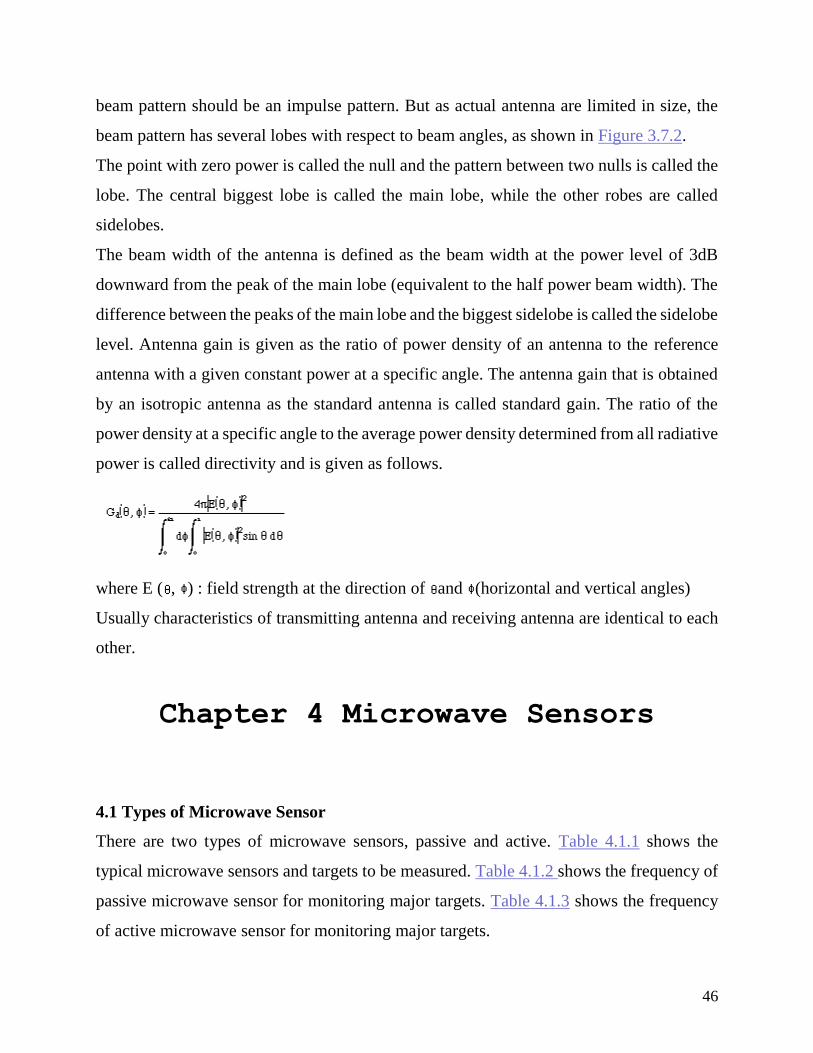
46

beam pattern should be an impulse pattern. But as actual antenna are limited in size, the

beam pattern has several lobes with respect to beam angles, as shown in Figure 3.7.2.

The point with zero power is called the null and the pattern between two nulls is called the

lobe. The central biggest lobe is called the main lobe, while the other robes are called

sidelobes.

The beam width of the antenna is defined as the beam width at the power level of 3dB

downward from the peak of the main lobe (equivalent to the half power beam width). The

difference between the peaks of the main lobe and the biggest sidelobe is called the sidelobe

level. Antenna gain is given as the ratio of power density of an antenna to the reference

antenna with a given constant power at a specific angle. The antenna gain that is obtained

by an isotropic antenna as the standard antenna is called standard gain. The ratio of the

power density at a specific angle to the average power density determined from all radiative

power is called directivity and is given as follows.

where E ( , ) : field strength at the direction of and (horizontal and vertical angles)

Usually characteristics of transmitting antenna and receiving antenna are identical to each

other.

Chapter 4 Microwave Sensors

4.1 Types of Microwave Sensor

There are two types of microwave sensors, passive and active. Table 4.1.1 shows the

typical microwave sensors and targets to be measured. Table 4.1.2 shows the frequency of

passive microwave sensor for monitoring major targets. Table 4.1.3 shows the frequency

of active microwave sensor for monitoring major targets.

47

Many of the earth observation satellites to be launched after 1992 are planned to have

microwave sensors onboard. Active sensors will be classified into more types in terms of

the target with respect to horizontal or vertical polarization.

4.2 Real Aperture Radar

Imaging radar as shown in Table 4.1.1 is classified further into Real Aperture Radar

(RAR) and Synthetic Aperture Radar (SAR). In this section RAR is explained.

RAR transmits a narrow angle beam of pulse radio wave in the range direction at right

angles to the flight direction (called the azimuth direction) and receives the backscattering

from the targets which will be transformed to a radar image from the received signals, as

shown in Figure 4.2.1.

Usually the reflected pulse will be arranged in the order of return time from the targets,

which corresponds to the range direction scanning.

The resolution in the range direction depends on the pulse width, as shown in Figure 4.2.2.

However if the pulse width is made small, in order to increase the resolution, the S/N ratio

of the return pulse will decrease because the transmitted power also becomes low.

Therefore, the transmitted pulse is modulated to chirp with a high power but wide band,

which is received through a matched filter, with reverse function of transmission, to make

the pulse width very narrow and high power as shown in Figure 4.2.3. This is called pulse

compression or de-chirping. By making the pulse compression, with an increase of

frequency f in transmission, the amplitude becomes times bigger, and the pulse width

becomes 1/TDf narrower. This method is sometime called range compression.

The resolution in the azimuth direction is identical to the multiplication of beam width and

the distance to a target. As the resolution of azimuth direction increases with shorter wave

length and bigger antenna size, a shorter wavelength and a bigger antenna is used for higher

azimuth resolution, as shown in Figure 4.2.4.

However as it is difficult to attach such a large antenna, requiring for example a 1 km

diameter antenna in order to obtain 25 meters resolution with L band ( =25 cm) and 100

km distance from a target, a real aperture radar therefore has a technical limitation for

improving the azimuth resolution.

48

4.3 Synthetic Aperture Radar

Compared to real aperture radar, Synthetic Aperture Radar (SAR) synthetically increases

the antenna's size or aperture to increase the azimuth resolution though the same pulse

compression technique as adopted for range direction. Synthetic aperture processing is a

complicated data processing of received signals and phases from moving targets with a

small antenna, the effect of which is to should be theoretically convert to the effect of a

large antenna, that is a synthetic aperture length, as shown as Figure 4.3.1.

The synthetic aperture length is the beam width by range which a real aperture radar of the

same length, can project in the azimuth direction.

The resolution in the azimuth direction is given by half of real aperture radar as shown as

follows.

Real beam width : = /D

Real resolution: L= R=Ls (synthetic aperture length)

Synthetic beam width : s = / 2Ls= D / 2R

Synthetic resolution : Ls = sR = D / 2

where :wavelength D: aperture of radar R: slant range

This is the reason why SAR has a high azimuth resolution with a small size of antenna

regardless of the slant range, or very high altitude of a satellite.

Figure 4.3.2 shows the basic theory of SAR or synthetic aperture processing including the

Doppler effect, matched filter and azimuth compression.

SAR continues to receive return pulses from a target during the time the radar projects the

beam to the target. In the meanwhile the relative distance between the radar and the target

changes with the movement of the platform, which produces a Doppler effect to modulate

a chirp modulation of received pulse. A matched filter corresponding to the reverse

characteristics of chirp modulation will increase the azimuth resolution of azimuth

direction. This is called azimuth compression.

In the case of SAR, unsuitability of satellite velocity and attitude will reduce the effect of

the Doppler effect. Therefore the satellite with SAR is required to be high, because the

49

correction for synthetic aperture processing due to instability at lower altitudes is very

difficult.

.4 Geometry of Radar Imagery

The incident angle of microwave to a target is the angle from the normal line while the

aspect angle is the supplementary angle as shown in Figure 4.4.1. The smaller the incident

angle , the larger the back scattering intensity .

Off nadir angle is the angle between the microwave and the nadir, while the depression

angle is the angle from the horizon, as shown in Figure 4.4.2. There occurs a geometric

distortion or shadow depending on the relationship between the off nadir angle and the

terrain relief, as shown in Figure 4.4.3 and Figure 4.4.4. Foreshortening occurs when the

ground range difference (horizontal distance X ) is reduced to the slant range difference

DR, because the slant range to the top and the bottom are not proportional to the horizontal

distances, as shown in the right hand example of Figure 4.4.5.

When the shortening becomes greater, the image of the top of a feature such as a mountain

will be closer to the antenna than the bottom, which causes loss of, the slope image, as

shown in the left hand example of Figure 4.4.5. This is called layover.

Such phenomena will occur when the terrain relief is greater and the off nadir angle is

smaller.

However for large off nadir angles, there will be a shadow area, as called radar shadow,

behind a hill or mountain, which makes the image very dark as shown in Figure 4.4.5.

The radar shadow will occur if the following relationship is satisfied.

+ > 90

where : slope angle of back slope

: off nadir angle

The slant range of the shadow is given as sec as shown in Figure 4.4.4.

4.5 Image Reconstruction of SAR

Raw data from SAR are records of backscattering in time sequence which are returned

from the ground targets. Return signal from a point P is recorded in the expanded range in

the range direction which is identical to the pulse width. In addition, the return signal from

50

a point P is also expanded in the azimuth direction because the point P continues to be

radiated by microwave pulses during the flight motion(see Figure 4.5.1).

Data processing to generate an image of gray tone corresponding to the backscattering

intensity of each point on the ground is called image reconstruction of synthetic aperture

radar (SAR). Figure 4.5.3 shows the flow of image construction of SAR.

The image reconstruction is divided into range compression and azimuth compression

which make compression of expanded signals in both range and azimuth directions into a

point signal. The compression is usually carried out by adopting Fourier transformation to

achieve convolution of received signals and a reference function.

The reference function of range compression is the complex conjugate of the transmitted

signal, while the reference of azimuth compression is a complex conjugate of the

modulated signal by chirp modulation.

The slant range to a point on the ground is expressed as the quadratic function of time with

respect to the movement of the platform. The change of the slant range is called range

migration. The first order term is called range walk resulting from the earth rotation,

while the second order term is called range curvature.

The range migration correction is to relocate the quadratic distribution (see Figure 4.5.4

(c)), in which range walk and range curvature may be separately processed.

In image reconstruction, there is a major problem, called speckle which is due to high

frequency noise, as seen in the example of Figure 4.5.2. In order to reduce the speckle,

mulch-look processing is applied in which range compression and azimuth compression

with respect to subdivided frequency domains are independently overlaid three or four

times termed the number of looks. Sometimes a median filter or local averaging may be

applied to reduce the speckle. The speckle will be reduced by the square root of the number

of looks, although the spatial resolution declines in proportion to the number of looks.

4.6 Characteristics of Radar Image

The main objective of microwave remote sensing is to estimate the property of objects by

interpreting the features of the radar image. Typical objects to be measured by microwave

remote sensing are mountainous land forms, subsurface geology, sea wind and waves etc.

51

In order to estimate these properties, it is very important to understand the effects of

microwave backscattering on the objects.

Two factors of microwave characteristics are of importance; frequency (or wavelength)

and polarization. In microwave remote sensing, various wavelengths (or frequency) such

as L band, C band, X band, P band etc. will be used ranging from millimeter wavelengths

(1 mm - 1cm) up to about 30 cm. According to the wavelength or frequency, specular

reflection will occur, so that the surface roughness can be detected if multi-frequency radar

images are compared.

Figure 4.6.1 and 4.6.3 are radar images of P band, L band and C band respectively with

HH polarization, in which the difference of wavelength or frequency will provide different

images.

Polarization is defined as the oscillating direction involved in an electric field. Usually

transmitted microwave and received microwave will have a choice between horizontal

polarization and vertical polarization. Therefore four combinations; HH, HV, VH and VV

can be used for SAR. The backscattering characteristics are also different with respect to

polarization. Figure 4.6.2 and 4.6.4 are HH, HV, and VV combinations respectively with

L band in which one can see different features.

In future, SAR systems with functions of multi-frequency and multi- polarization will be

onboard earth observation satellites.

4.7 Radar Images of Terrains

The biggest effect of microwave backscattering on variations in the radar image is due to

terrain features. It is larger than the effect of permittivity. Particularly the effect of incident

beam angle in terms of off nadir angle and terrain slope will produce various effects such

as foreshortening, layover and shadow as already explained in section 4.4.

Normally in the closer range from SAR, called near range, layover may occur while in

the far range more shadow may be seen. This means that care should be taken with the

flight direction and range direction in interpretation of terrain features.

Figure 4.7.1 shows an example of a SAR image of SEASAT around the mountainous areas

of Geneva, Switzerland.

52

Figure 4.7.2 shows the effect of terrain and off nadir angle on foreshortening, layover and

shadow.

Usually foreshortening and layover appear as a bright response around the summit or ridge,

while shadow appears black without any information in the shadow area.

As seen in the figure, the effect of microwave back scattering can be better seen along the

track or azimuth direction than in the cross track direction.

By interpreting the radar image, land form classification, lineament analysis, mineral

resources exploration, monitoring of active volcanoes, land slide monitoring, geological

structure analysis and so on can be carried out.

Two parallel flights may produce a stereo pair which will offer the elevation information

on terrain features. Recent work is Canada has demonstrated that terrain elevation

information can also be derived from the use of interferometry with a single flight line.

4.8 Microwave Radiometer

As indicated in section 3.4, a part of the microwave is also radiated by thermal radiation

from the objects on the earth. Microwave radiometers or passive type microwave sensors

are used to measure the thermal radiation of the ground surface and/or atmospheric

condition.

Brightness temperature measured by a microwave radiometer is expressed by Reyleigh-

Jean's law (see 1.7), which is the resultant energy of thermal radiation from the ground

surface and the atmospheric media. Multi-channel radiometers with multi- polarization are

used to avoid the influences of unnecessary factors to measure the specific physical

parameter.

Figure 4.8.1 shows the sensitivity of physical parameters in oceanography with respect to

frequency and the optimum channels as arrow symbols.

Figure 4.8.2 shows two typical microwave scanning radiometers; the conical scanning

type and the cross track scanning type. The former is used for the microwave channel

which is influenced by the ground surface, while the latter is used for the channel which

can be neglected by the influence of the ground surface.

53

The most simple radiometer is the total power radiometer, as shown in Figure 4.8.3. This

system has a mixer to enable it to mix high frequency of a local oscillator in order to

amplify the high signal after transforming to a low frequency. However the influence of

system gain variation cannot be neglected in this system.

The Dicke radiometer can reduce the influence of system gain variation by introducing a

switch generator which allows it to receive the antenna signal and noise source of constant

temperature, alternatively of which antenna signal can be detected later on, synchronously

with the switch generator.

The zero-balance Dicke radiometer can reduce the influence of system gain variation and

increase the sensitivity further by adding a noise generator to the Dicke radiometer in order

to increase the sensitivity about two times higher than total power radiometer.

4.9 Microwave Scatterometer

Microwave scatterometers can measure the received power of surface backscattering

reflected from the surface of objects. According to a narrow definition, a microwave

scatterometer may be a space borne sensor to measure the two dimensional velocity vectors

of the sea wind, while according to the wider definition, it also involves air-borne sensors,

as well as ground based sensors to measure the surface backscattering as well as volume

scattering, such as rain radar.

Microwave scatterometers are classified as two types, pulse type and continuous wave

type (CW). The pulse type uses wide band which has restrictions in obtaining a license to

operate and in avoid obstructions. CW type has the advantage that the band width can be

reduced to 1/100 times that of the pulse type and the price becomes cheaper.

SEASAT-SASS (Seasat-A Satellite Scatterometer) is one of the typical scatterometers.

SASS has four fixed antennas to transmit the pulse in a fan beam of 14.5 GHz to four

different angles, and to receive the backscattering in subdivided cells through a Doppler

filter. Figure 4.9.1 shows the four beam patterns and the incident angles. In accordance

with the satellite flight, the same cell of sea area can be observed from both fore beam and

aft beam with 90 different angle, which enables the determination of wind direction and

wind velocity.

54

Figure 4.9.2 shows a ground based microwave scatterometer with a rotation system.

ERS-1-AMI Wind Mode (European Remote Sensing Satellite-1-Active Microwave

Instrument) and ADEOS-NSCAT (Advanced Earth Observation System-1 NASA

Scatterometer) will be available for measurement of velocity vectors of the sea wind with

three antennas looking fore, side and aft directions.

Table 4.9.1 compares the basic functions of ERS-AMI Wind Mode and ADEOS-NSCAT.

Both have functions to measure wind velocity of the sea wind with an accuracy of 2 m/s or

10 % of the waveheight , and wind direction with an accuracy of 20 .

4.10 Microwave Altimeter

Microwave altimeters or radar altimeters are used to measure the distance between the

platform (usually satellite or aircraft) and the ground surface. Some applications of

microwave altimetry are in ocean dynamics of the sea current, geoid surveys, and sea ice

surveys. Therefore, precise measurement of the satellite orbit and the geoid should be

carried out.

The principle of satellite altimetry is shown in Figure 4.10.1. The ground height or the sea

surface height is measured from the reference ellipsoid. If the altitude of the satellite Hs

is given as the height from the reference ellipsoid, the sea surface height HSSH is

calculated as follows.

HSSH = Hs - Ha where Ha : measured distance between satellite and the sea surface.

The sea surface height is also represented by the geoid height Hg that is measured between

the geoid surface and the reference ellipsoid and the sea surface topography DH is given

as follows.

HSSH = Hg + ΔH

The sea surface topography results from ocean dynamics such as sea current, wave height,

tidal flow etc., which can be determined if the geoid height Hg is given. The distance

between a satellite and the ground surface or sea surface; Ha, is measured on the basis of

the travel time of the transmitted microwave pulses. From the time (t=0), when the first

edge of pulse arrives at the surface, to the time (t= ) when the end edge of a pulse with a

width of arrives at the surface, the received power increases linearly as shown in Figure

55

4.10.2. The received pulses are composed of echoes from various parts of the sea surface.

Therefore the travel time from a satellite to the sea surface can be calculated by averaging

the received pulses. Pulse compression techniques will be also applied (see 4.2) in order to

obtain a high frequency pulse for improvement of the resolution.

Ocean wave height can be estimated if the relation between the average scattering

coefficient and elapsed time as seen in the different gradients in Figure 4.10.3 is taken into

account.

4.11 Measurement of Sea Wind

Measurement of the sea wind is not made directly but indirectly from two processes, that

is, the microwave scattering from the sea surface and relationship between sea wind and

wave height.There are two methods for measurement of sea wind.

a. to estimate the backscattering coefficient using a microwave scatterometer

b. to measure the brightness temperature using a microwave radiometer

The following three models are used to estimate the backscattering coefficient in the case

of a microwave scatterometer.

a. specular point model

b. Bragg model

c. composite surface model

Figure 4.11.1 shows the relationship between backscattering cross section and the incident

angle which has been obtained from the actual measurement. The specular point model can

be applied to the region A in the figure, with the incident angle from 0 to 25 , where the

sea clutter or sea roughness is much larger than the microwave wavelength. In this case,

the backscattering coefficient is proportional to the resultant probability density of x and

y components of the gradient.

The Bragg model can be applied to the region B in the figure with the incident angle larger

than 25 , where ¡ decreases very gently except near 90 . This is called Bragg scattering

which can be seen under the condition when the wavelengths of microwave and the sea

wave have a similar spectrum. The ideal condition for Bragg scattering has the range from

25 to 65 with the wavelength of the capillary wave being from 1 cm to a few cm.

56

However, the actual sea surface is a composite of capillary waves and gravity waves for

which the composite surface model has been developed but not yet verified theoretically.

The second procedure is to estimate the sea surface condition from the backscattering

coefficient . Figure 4.11.2 shows the correlation between variance of wave slope, S , and

the wind velocity measured by Cox and Munk, which can be applied for the specular point

model when is given as a function of S . In the case of >25, it is found that the sea wind

is proportional to the spectral density, but the models are still under development. Figure

4.11.3 shows the distribution of wind velocity and wind direction that was measured by

SASS (Seasat-A Satellite Scatterometer) for the typhoon on Oct. 2, 1978. In the case of the

microwave radiometer, the sea wind can be computed from the brightness temperature

using the fact that the emissivity is a function of complex permittivity with parameters of

salinity, sea clutter, sea temperature and bubbles. Two algorithms have been developed by

Wentz and Wilheit for Seasat- SMMR for the sea wind velocity.

4.12 Wave Measurement by Radar

While ordinary measurements of waves by a wave gauge are used for a time variation of

wave height at a point, remote sensing techniques gives information over a broader area.

There are two methods of wave measurement used in remote sensing. a. space borne

sensors such as SAR and microwave altimeter b. ground base radar such as X band radar

and HF Doppler radar

As space borne sensors have a lower resolution (of the order of a few ten meters to a few

kilometers), large size currents, typhoons over wide areas, global wave distribution, etc.,

will be better monitored by these systems.

On the other hand, ground based radar is suitable for monitoring the waves in near offshore

or shallow zones, with the wave field of a few ten centimeters to a few hundred meters.

Figure 4.12.1 shows the distribution of average significant wave height which was

measured by GEOSAT-ALT, with an accuracy of +-0.5 m or 10 % of the wave height.

Space borne SAR and ground based X band radar are used for measurement of reflectivity

from the sea clutter at similar wavelengths to the sensors based on Bragg scattering (see

4.11).

57

Figure 4.12.2 explains the effect of capillary waves with respect to slope change or

incident angle for Bragg scattering and wave height.

Figure 4.12.3 shows the sea surface conditions measured by SAR and X band radar. The

measurement of wave direction and wave length is already operational as a ship borne radar

but the measurement of wave height is still being researched. HF Doppler radar using high

frequency band (10-100 m) , which is longer than microwave can measure the Bragg

scattering from the sea clutter with wave lengths of 5-50 m.

Wave conditions such as wave direction, significant wave height, predominant wave,

current etc. of wind waves with longer wave lengths, can be measured by using the Doppler

effect with phase velocity of the wave crest. HF Doppler radar is already operational.

Chapter 5 Platforms

5.1 Types of Platform

The vehicle or carrier for remote sensors are borne is called the platform. Typical

platforms are satellite and aircraft, but they can also include radio controlled airplanes,

balloons, kites for low altitude remote sensing, as well as ladder trucks or "cherry pickers"

for ground investigations.

Table 5.1.1 shows various platforms, altitudes and objects being sensed. Platforms with the

highest altitude are geosynchronous satellites such as the Geosynchronous Meteorological

Satellite (GMS), which has an altitude of 36,000 km at the Equator. Most of the earth

observation satellites, such as Landsat, SPOT, MOS etc. are at about 900 km altitude with

a sun synchronous orbit.

From lower orbit, there are space shuttle (240-280 km), radio sonde ( - 100 km), high

altitude jet-plane ( 10,000 m), low or middle altitude plane (500-8,000 m), radio controlled

plane ( - 500 m) and so on.

58

The key factor for the selection of a platform is the altitude which determines the ground

resolution if IFOV (instantaneous field of view) of the sensor is constant, where

= H

The selection of platform also depends on the purpose which is sometime requested for

example a constant altitude is required for aerial surveys, while various altitudes are needed

to survey vertical atmospheric distribution, for example.

For aerial photogrammetry, the flight path is strictly controlled to meet the requirement of

geometric accuracy. However, helicopter or radio controlled planes are used for a free path

approach, for example in disaster monitoring.

5.2 Atmospheric Condition and Altitude

Atmospheric condition is different depending on the altitude. This factor must be

considered in the selection of platforms or sensors. In this section, air pressure, air density

and temperature are considered.

Dependence of air pressure on altitude is based on the hydro-static equilibrium of balance

between the vertical pressure of the atmosphere and gravity.

The atmospheric constituents without water vapor are assumed constant in volume ratio

with 78.08 % nitrogen, 20.95 % oxygen, and argon 0.93 % up to about 100 km regardless

of time and place. It gives an average molecular weight at 28.97 for the atmosphere and

the average molecular mass of 4.810 x 10 kg.

When temperature is constant with respect to altitude, the air pressure decreases as an

exponential function, which gives about an 8 km altitude for a decrease of air pressure to

1/e, as shown in Figure 5.2.1.

However, since the actual atmosphere varies in temperature with altitude as shown in

Figure 5.2.2, the air pressure can be calculated from the hydro-static equilibrium with a

given temperature.

59

For general purposes, the standard model atmosphere has been specified with respect to

the average temperature distribution and the vertical air pressure. Also the average model

with respect to latitude and season has been specified, although the actual temperature

sometimes has a difference of 10 - 20 K. Therefore the measurement of temperature using

radio-sonde is necessary for high accuracy. The vertical structure of the atmosphere is

composed of the following layers.

Troposphere : from the ground surface to 10 - 17 km,

Stratosphere : from 10 - 17 km to about 50 km

Mesosphere : from about 50 km to about 90 km

Thermosphere : from about 90 km to 500 km

The classification of the above layers depends on the distribution of thermal energy and

thermal transportation. The vertical decrease of temperature in the troposphere is 9.8 K km

for dry atmosphere, but 6.5 K km for the actual atmosphere because of water vapor. The

boarder between the troposphere and the stratosphere is called tropopause. The tropics

tropopause is rather constant at 17 km in altitude while the middle latitude tropopause

depends on seasonal change and jet stream with 10 - 17 km in altitude as shown in Figure

5.2.3.

5.3 Attitude of Platform

The geometric distortion depends on not only the geometry of the sensor but also the

attitude of the platform. Therefore it is very important to measure the attitude of the

platform for the consequent geometric correction.

The attitude of the platform is classified by the following two components.

a. Rotation angles around the three axes ; roll, pitch and yaw b. Jitter ; random and

unsystematic vibration which cannot be measured.

The rotation angles ; roll ( ), pitch ( ) and yaw ( ) are defined as the rotation angles around

the flight direction, the main wing and the vertical line respectively, as shown in Figure

5.3.1. Figure 5.3.2 show the satellite attitude parameters.

For a frame camera, the rotation angles are single values common to a full scene of aerial

photograph, while for a line scanner the attitude changes as a function of line number or

60

time. In the case of satellites, the variation of the position and the attitude will be

continuous, though in case of aircraft, the variation will not always be smooth, which

makes the geometric correction more difficult.

The typical attitude sensors for aircraft are as follows.

- Speedometer

- altimeter

- gyro compass (for attitude measurement)

- Doppler radar (for measurement of altitude)

- GPS (for positioning )

- gyro horizon

- TV camera

- flight recorder

The attitude sensors for satellites are introduced in section 5.4.

5.4 Attitude Sensors

Attitude control of a satellite is classified by two methods ; spin control and three axis

control. The former method is usually adopted for geosynchronous meteorological

satellites which itself rotates itself together with rotating scanner. The latter method is

mainly adopted for earth observation satellites such as Landsat which needs accurate look

angle in the direction of the earth.

The spin control is rather simple but has a low S/N ratio, while the three axis control is

more complex, but has a high S/N.

Figure 5.4.1 shows the typical types of attitude measurement sensors, which are used for

different purposes.

A gyro-compass is used for measurement of attitude variation over a short interval. Earth

sensor detects the radiation of CO2 with in the wavelength range of 14 - 16 mm emitted

from the rim of the earth, from which two axis attitude of roll and pitch can be measured

with an accuracy of 0.3 - 1 degree, as shown in Figure 5.4.2. If the earth sensor is combined

with a sun sensor and gyro-compass, the three axis attitude can be measured with higher

accuracy of 0.1 - 0.3 degree. Magnetic sensors can measure the three axis attitude but with

61

a slightly low an accuracy. The responsivity of the above sensors is 2 Hz at maximum. If

the high frequency attitude such as jitter is to be measured, the angular displacement

sensor (ADS) is necessary.

The angular displacement sensor of Landsat 4 and 5 has a responsivity of 2 - 18 Hz. The

highest accuracy of attitude can be achieved by the star sensor. For example, the standard

star tracker (SST) on board Landsat 4 and 5 will measure an accurate attitude from the

image of stars acquired by an image dissector with a reference of about 300 star catalogue

up to the sixth grade stars stored in an on board computer. The accuracy of SST is about

+- 0.03 degree (3 ).(3 standard deviations).

In case of the space shuttle, the star sensor has a lower accuracy with only about a 50 star

catalog compared to the SST, because the space shuttle does not need the higher attitude

control when it returns to the troposphere.

5.5 Orbital Elements of Satellite

A set of numerical values to define an orbit of a satellite or planet are called orbital

elements. The independent orbital elements of the earth observation satellite are six

elements of the Keplerian orbit.

A satellite can be considered to rotate around the earth in a plane, called the orbital plane,

because the influence of gravity of the moon and the sun can be neglected as compared

with the gravity of the earth.

A point in space can be expressed in the equatorial coordinate system as follows. The

origin of equatorial coordinate system is the center of the earth.

The reference great circle : the equatorial plane

The origin of astronomical longitude (right ascension) : the vernal equinox

The astronomical longitude (right ascension) : 0 - 24 hours to the east from the vernal

equinox

The astronomical latitude (declination) : angle from the equatorial plane ( +90 degree in

the north pole ; -90 degree in the south pole)

The six elements of Keplerian orbit are ;

62

(1) The semi-major axis (A):

(2) Eccentricity of orbit (e) :

(3) Inclination angle (i) :

(4) Right ascension of ascending node (h)

(5) Argument of perigee (g)

(6) Time of passage of the perigee ( )

Figure 5.5.1 shows the above elements. The shape and size of an orbit can be defined by A

and e, while the orbit plane can be defined by i and h. The longer axis of the orbit ellipse

can be determined by g. The position of a satellite can be located by T.

Sometime the orbital elements are replaced by three dimensional geocentric coordinates

and velocity for numerical analysis instead of the elements of the the Keplerian orbit.

Table 5.5.1 shows the relationship between the elements of the Keplerian orbit and the

geocentric.

5.6 Orbit of Satellite

The orbit of a satellite is referred to by several names with respect to orbit figure,

inclination, period and recurrence as shown in Figure 5.6.1.

The circular orbit is the most basic orbit and is explained as follows. The orbit can be

expressed as the polar coordinates (r, ).

r = r e + h s = 0 t

where re : radius of the earth 6,378,160 m

hs : altitude of satellite

t : time

0 : angular velocity

The angular velocity and the period are expressed as follows.

where : gravity constant ; 3.986005

a. Geosynchronous orbit

63

The orbit with the same earth rotation rate (h24 = the sidereal day ; 86164.1 sec) is called

an earth synchronous orbit or geosynchronous orbit. The geosynchronous orbit with an

inclination of i = 0 is called a geostationary orbit because the satellite looks stationary over

the equator from a ground surface view. As such, a geostationary satellite is useful for

covering wide areas. Many meteorological satellites and communication satellites are

geosynchronous types.

b. Sun synchronous orbit

Most earth observation satellites, such as Landsat, with lower altitudes have sun

synchronous and semi-recurrent orbits. The sun synchronous orbit can be defined as the

orbit in which the orbital plane rotates in a year in unison with the one revolution / year

apparent motion of the sun. The model precession rate , is a function of inclination i, orbit

altitude hs and orbital period T as shown in Figure 5.6.2. As seen in the figure, the sun

synchronous orbit has W=1 (revolution / year). For example, in case of i = 100 degree, the

altitude of the sun synchronous orbit is about 1,200 km with about 108 minutes of orbit

period. The advantage of the sun synchronous orbit is that the observation conditions can

be kept with a constant solar incident angle.

c. Semi-recurrent orbit

While the recurrent orbit can be defined as the orbit which returns to the same nadir point

in a day, the semi-recurrent orbit returns to the same nadir point in N days repetition (N>1),

which is much better for covering all of the earth than the recurrent orbit.

5.7 Satellite Positioning Systems

There are two methods for positioning a satellite: distance measurement from the ground

station, and GPS as shown in Figure 5.7.1. As GPS is explained in 6.8, the former method

will be explained here. The measurement of distance for satellite positioning is called the

range and range rate system, by which the time of a radio wave transmitted between the

ground station and a transponder onboard the satellite is measured with the Doppler

frequency. It enables the distance or range and the range rate to be measured. The accuracy

of the range and range rate is a few meters/second, respectively. The accuracy depends on

64

the parameters of frequency, signal, the location of the ground station, coordinate system,

time measurement system, reflection in the troposphere and the ionosphere etc.

The position of a satellite by the range and range rate method is limited only near the

ground station and is also discrete. In order to determine the satellite orbit in a time

sequential function, it is necessary to construct a model.

A primitive model is a parabolic curve based on the third theory of Kepler that defines

the motion of two bodies in space, termed the two body problem, under the law of

universal gravitation. The parabolic curve can be expressed with the six elements of the

Keplerian orbit.

However in reality there are influences from other planets, which results in departure from

the parabolic curve. This is called the perturbation.

There are two methods to determine the precision for an body problem (n>2); the numerical

integral calculation, which has high accuracy but is time consuming and the analytical

method with a lower accuracy but faster calculation, as shown in Table 5.7.1.

The satellite position in an orbit will be determined at certain time intervals, from which

the orbit at an arbitrary time can be interpolated by the least square method for high order

polynomials or by Lagrange's interpolation method.

5.8 Remote Sensing Satellites

A satellite with remote sensors to observe the earth is called a remote sensing satellite or

earth observation satellite. Meteorological satellites are sometimes discriminated from the

other remote sensing satellites.

Remote sensing satellites are characterized by their altitude, orbit and sensors. The main

purpose of the geosynchronous meteorological satellite (GMS) with an altitude of 36,000

km is meteorological observations, while Landsat with an altitude of about 700 km, in a

polar orbit, is mainly for land area observation.

NOAA AVHRR with an altitude of 850 km in a polar orbit is mainly designed for

meteorological observation but is also successfully used for vegetation monitoring.

In future some remote sensing satellites will have large payloads with many kinds of multi-

purpose sensors, such as the polar orbit platform (POP) project under the international

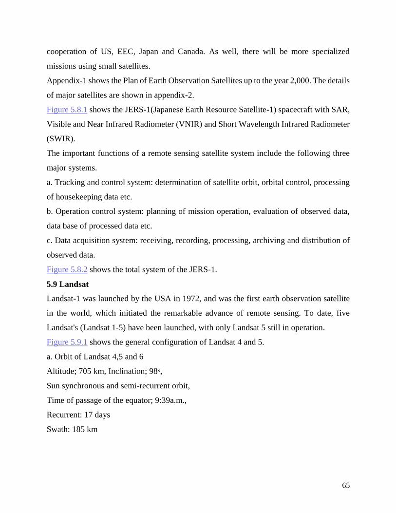
65

cooperation of US, EEC, Japan and Canada. As well, there will be more specialized

missions using small satellites.

Appendix-1 shows the Plan of Earth Observation Satellites up to the year 2,000. The details

of major satellites are shown in appendix-2.

Figure 5.8.1 shows the JERS-1(Japanese Earth Resource Satellite-1) spacecraft with SAR,

Visible and Near Infrared Radiometer (VNIR) and Short Wavelength Infrared Radiometer

(SWIR).

The important functions of a remote sensing satellite system include the following three

major systems.

a. Tracking and control system: determination of satellite orbit, orbital control, processing

of housekeeping data etc.

b. Operation control system: planning of mission operation, evaluation of observed data,

data base of processed data etc.

c. Data acquisition system: receiving, recording, processing, archiving and distribution of

observed data.

Figure 5.8.2 shows the total system of the JERS-1.

5.9 Landsat

Landsat-1 was launched by the USA in 1972, and was the first earth observation satellite

in the world, which initiated the remarkable advance of remote sensing. To date, five

Landsat's (Landsat 1-5) have been launched, with only Landsat 5 still in operation.

Figure 5.9.1 shows the general configuration of Landsat 4 and 5.

a. Orbit of Landsat 4,5 and 6

Altitude; 705 km, Inclination; 98 ,

Sun synchronous and semi-recurrent orbit,

Time of passage of the equator; 9:39a.m.,

Recurrent: 17 days

Swath: 185 km

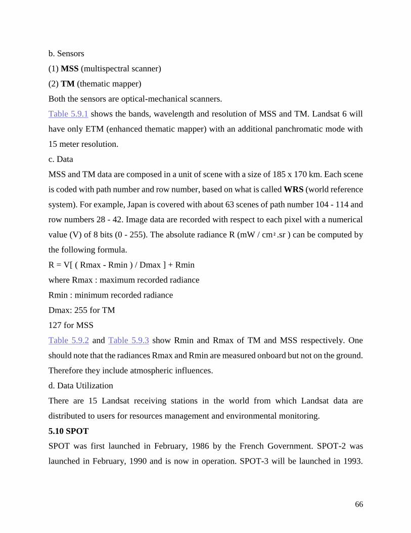
66

b. Sensors

(1) MSS (multispectral scanner)

(2) TM (thematic mapper)

Both the sensors are optical-mechanical scanners.

Table 5.9.1 shows the bands, wavelength and resolution of MSS and TM. Landsat 6 will

have only ETM (enhanced thematic mapper) with an additional panchromatic mode with

15 meter resolution.

c. Data

MSS and TM data are composed in a unit of scene with a size of 185 x 170 km. Each scene

is coded with path number and row number, based on what is called WRS (world reference

system). For example, Japan is covered with about 63 scenes of path number 104 - 114 and

row numbers 28 - 42. Image data are recorded with respect to each pixel with a numerical

value (V) of 8 bits (0 - 255). The absolute radiance R (mW / cm .sr ) can be computed by

the following formula.

R = V[ ( Rmax - Rmin ) / Dmax ] + Rmin

where Rmax : maximum recorded radiance

Rmin : minimum recorded radiance

Dmax: 255 for TM

127 for MSS

Table 5.9.2 and Table 5.9.3 show Rmin and Rmax of TM and MSS respectively. One

should note that the radiances Rmax and Rmin are measured onboard but not on the ground.

Therefore they include atmospheric influences.

d. Data Utilization

There are 15 Landsat receiving stations in the world from which Landsat data are

distributed to users for resources management and environmental monitoring.

5.10 SPOT

SPOT was first launched in February, 1986 by the French Government. SPOT-2 was

launched in February, 1990 and is now in operation. SPOT-3 will be launched in 1993.

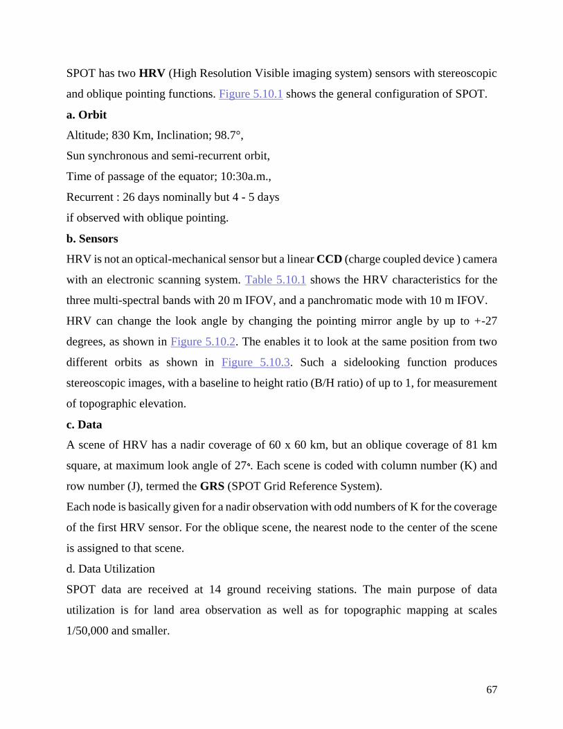
67

SPOT has two HRV (High Resolution Visible imaging system) sensors with stereoscopic

and oblique pointing functions. Figure 5.10.1 shows the general configuration of SPOT.

a. Orbit

Altitude; 830 Km, Inclination; 98.7°,

Sun synchronous and semi-recurrent orbit,

Time of passage of the equator; 10:30a.m.,

Recurrent : 26 days nominally but 4 - 5 days

if observed with oblique pointing.

b. Sensors

HRV is not an optical-mechanical sensor but a linear CCD (charge coupled device ) camera

with an electronic scanning system. Table 5.10.1 shows the HRV characteristics for the

three multi-spectral bands with 20 m IFOV, and a panchromatic mode with 10 m IFOV.

HRV can change the look angle by changing the pointing mirror angle by up to +-27

degrees, as shown in Figure 5.10.2. The enables it to look at the same position from two

different orbits as shown in Figure 5.10.3. Such a sidelooking function produces

stereoscopic images, with a baseline to height ratio (B/H ratio) of up to 1, for measurement

of topographic elevation.

c. Data

A scene of HRV has a nadir coverage of 60 x 60 km, but an oblique coverage of 81 km

square, at maximum look angle of 27 . Each scene is coded with column number (K) and

row number (J), termed the GRS (SPOT Grid Reference System).

Each node is basically given for a nadir observation with odd numbers of K for the coverage

of the first HRV sensor. For the oblique scene, the nearest node to the center of the scene

is assigned to that scene.

d. Data Utilization

SPOT data are received at 14 ground receiving stations. The main purpose of data

utilization is for land area observation as well as for topographic mapping at scales

1/50,000 and smaller.

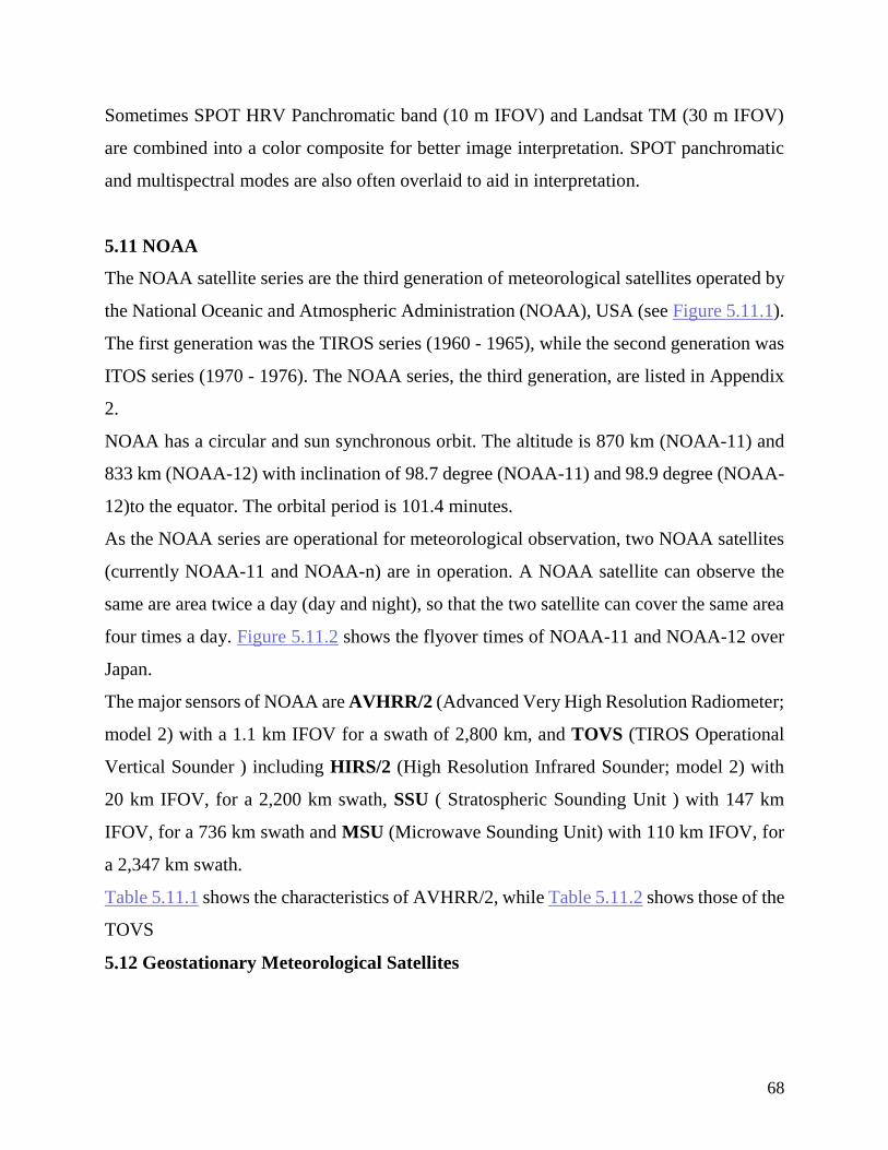
68

Sometimes SPOT HRV Panchromatic band (10 m IFOV) and Landsat TM (30 m IFOV)

are combined into a color composite for better image interpretation. SPOT panchromatic

and multispectral modes are also often overlaid to aid in interpretation.

5.11 NOAA

The NOAA satellite series are the third generation of meteorological satellites operated by

the National Oceanic and Atmospheric Administration (NOAA), USA (see Figure 5.11.1).

The first generation was the TIROS series (1960 - 1965), while the second generation was

ITOS series (1970 - 1976). The NOAA series, the third generation, are listed in Appendix

2.

NOAA has a circular and sun synchronous orbit. The altitude is 870 km (NOAA-11) and

833 km (NOAA-12) with inclination of 98.7 degree (NOAA-11) and 98.9 degree (NOAA-

12)to the equator. The orbital period is 101.4 minutes.

As the NOAA series are operational for meteorological observation, two NOAA satellites

(currently NOAA-11 and NOAA-n) are in operation. A NOAA satellite can observe the

same are area twice a day (day and night), so that the two satellite can cover the same area

four times a day. Figure 5.11.2 shows the flyover times of NOAA-11 and NOAA-12 over

Japan.

The major sensors of NOAA are AVHRR/2 (Advanced Very High Resolution Radiometer;

model 2) with a 1.1 km IFOV for a swath of 2,800 km, and TOVS (TIROS Operational

Vertical Sounder ) including HIRS/2 (High Resolution Infrared Sounder; model 2) with

20 km IFOV, for a 2,200 km swath, SSU ( Stratospheric Sounding Unit ) with 147 km

IFOV, for a 736 km swath and MSU (Microwave Sounding Unit) with 110 km IFOV, for

a 2,347 km swath.

Table 5.11.1 shows the characteristics of AVHRR/2, while Table 5.11.2 shows those of the

TOVS

5.12 Geostationary Meteorological Satellites

69

Geostationary meteorological satellites are launched under the WWW (World Weather

Watch) project organized by the WMO (World Meteorological Organization), which will

cover all the earth with five satellites as shown in Figure 5.12.1.

The five geostationary meteorological satellites are METEOSAT (ESA), INSAT (India),

GMS (Japan), GOES-E (USA) and GOES-W (USA). The schedules for these satellites

are shown in Appendix 1.

As of 1991, METEOSAT-5, INSAT-1D, GMS-4 and GOES-7 are in operation.

GMS-4 has a sensor called VISSR (Visible and Infrared Spin Scan Radiometer) with two

bands of visible and thermal infrared. The VISSR scans four lines for the visible band and

a line for the thermal band simultaneously from the north to the south, which takes 25

minutes to cover the semi-sphere as shown in Figure 5.12.2.

The total scan lines are 10,000 lines for the visible band and 2,500 lines for the thermal

band.

GMS has a data collection platform (DCP) system to collect various information, not only

from the ground station, but also from the stations on the sea as shown in Figure 5.12.3.

The image data are transmitted to the ground station in a high resolution mode of S-VISSR

signals, and also in a low resolution mode of WEFAX, which can be received by cheaper

and simpler receiving facilities. Some statistical data such as histograms, cloud volumes,

sea surface temperatures, wind distribution and so on, are recorded in the archives

including the ISCCP (International Satellite Cloud Climatology Project) data set.

5.13 Polar Orbit Platform

The Polar orbit platform (POP) is a newly designed system for the 21st century, intended

to establish a longer life space infrastructure with multiple sensors as well as multiple uses,

when compared with the existing satellites which are used for a limited period and purpose.

POP is composed of a main space station, a space shuttle and an inter-orbital vehicle as

shown in Figure 5.13.1, by which exchange of mission equipments and repair of the form

will be possible.

70

POP is made of a module structure with ORU (Orbital Replacement Unit) for replacement

of mission parts and battery. Such functions of POP will make the system large in size and

payload, but long in life.

Japanese ADEOS (Advanced Earth Observation Satellite) as shown in Table 5.13.1 is not

POP a but is designed for a future type platform of earth observation satellite with the

function of data relay. ADEOS is characterized by the multiple sensors of OCTS (Ocean

Color and Temperature Scanner by NASDA), AVNIR (Advanced Visible and Near

Infrared Radiometer by NASDA), and AO (Applications of Opportunity) sensors such as

NSCAT, TOMS, IMG, POLDER, and ILAS .

At present the space station project is delayed and cut back to a smaller system without

orbital services. For example, NASA EOS-a and b, ESA POEM-1 and 2 will be launched

at the end of the 20th century for earth environmental monitoring.

Chapter 6 Data used in Remote

Sensing

6.1 Digital Data

Images with a continuous gray tone or color, like a photograph are called analog images.

On the other hand, a group of divided small cells, with integer values of average intensity,

the center representing the cell's value, is called a digital image. The spatial division into

a group of cells is called sampling as illustrated in Figure 6.1.1, while conversion of analog

images into integer image data is called quantization as illustrated in Figure 6.1.2 and

6.1.3.

71

An individual divided cell is called a pixel (picture cell). The shape of the cell is usually

square for easy use in a computer, though triangular or hexagonal can also be considered.

A digital image has coordinates of pixel number, normally counted from left to right, and

line number, normally counted from top to bottom.

The most important factor in sampling is pixel size or sampling frequency. If the pixel size

is large or the sampling frequency is long, the appearance of the image becomes worse,

while in the reverse case the data volume becomes very large. Therefore the optimum

sampling should be carefully considered.

Shannon's sampling theorem, for specifying the optimum sampling, is given as follows.

"There will be no loss of information if sampling is taken with a half frequency of the

maximum frequency involved in the original analog frequency wave."

Let the analog intensity be f and the unit intensity v(>0) as divider in quantization. Let the

quantized intensity be fd, fd is given by n as illustrated in Figure 6.1.2. The difference

between f and fd is called quantization error.

The question is how to determine the number of quantization levels or the unit intensity as

divider. If the number of levels is too small, the quantization error will increase. In the

reverse, the data volume increases with informationless data because of the noise level, as

shown in Figure 6.1.3.

For example in Figure 6.1.3, the quantization should be divided by a level larger than that

of the noise. In this example, four levels would be an appropriate quantization.

6.2 Geometric Characteristics of Image Data

Remote sensing data are data digitized by a process of sampling and quantization of the

electro-magnetic energy which is detected by a sensor. In this section, geometric

characteristics of sampling are described, while radiometric characteristics by quantization

are explained in 6.3.

IFOV (Instantaneous Field Of View) is defined as the angle which corresponds to the

sampling unit as shown in Figure 6.2.1. Information within an IFOV is represented by a

pixel in the image plane.

72

The maximum angle of view which a sensor can effectively detect the electro magnetic

energy, is called the FOV (Field Of View). The width on the ground corresponding to the

FOV is called the swath width.

The minimum detectable area, or distance on the ground is called the ground resolution.

Sometimes the projected area on the ground corresponding to a pixel or IFOV is also called

the ground resolution.

In remote sensing, the data from a multiple number of channels or bands which divide the

electromagnetic radiation range from Ultra Violet to Radio Waves are called multi-

channel data, multi-band data or multi- spectral data.

In general, multi-channel data are obtained by different detectors as shown in Figure 6.2.2.

Because the detectors are located at slightly different positions, and the light path of

different wavelengths is a little different from each other, the images of multi-channel data

are not identical in geometric position. To correct such geometric errors between channels

is called registration.

The term registration is also used for registration of multi-temporal (or multi-date) images.

6.3 Radiometric Characteristics of Image Data

Electromagnetic energy incident on a detector is converted to an electric signal and then

digitized. In this quantization process, the relationship between the input signal and the

output signal is generally represented as shown in Figure 6.3.1. In this curve the left part

corresponds to the insensitive area, with less response, while the right part is the saturated

area with almost constant output regardless of the input intensity.

In the central part, there is almost a linear relationship between the input and the output.

The approximation to a linear relationship is called linearity. The range of the linear part

or the ratio of maximum input to minimum input is called the dynamic range, which is

usually expressed in dB (see 2.2).

One should be careful of the noise level in the case of quantization, as explained in 6.1.

The ratio of effective input signal S to the noise level N is called the S/N ratio (signal to

noise ratio), which is given as follows.

S / N ratio = 20 log10 (S/N) [dB]

73

In conclusion, quantization is specified by the dynamic range and the S/N ratio.

Information contained in digitized image data are expressed by bit (binary digit) per pixel

per channel.

A bit is a binary number, that is 0 or 1. Let the quantization level be n, then the information

in terms of bits is given by the following formula.

log2 n (bit)

In remote sensing, the quantization level is normally 6, 8 or 10 bits as shown in Table 6.3.1.

For computer processing, the unit of byte (1 byte = 8 bits;integer value 0-255 ; 256 gray

levels) is much more convenient. Therefore remote sensing data will be treated as one or

two byte data.

The total data volume of multi-channel data per scene is computed as follows.

Data Volume(byte) = (line number) x (pixel number) x (channel number) x (bits) /8

Output data usually corresponds to the observed radiance detected by the sensor. The

absolute radiance is converted by a linear formula from the observed radiance (see 9.1).

The parameters are usually listed in the User's Manual for the particular remote sensing

system.

6.4 Format of Remote Sensing Image Data

Multi-band image data are represented by a combination of spatial position (pixel number

and line number) and band.

The data format for multi-band images is classified into the following three type, as shown

in Figure 6.4.1.

a) BSQ format (band sequential) image data (pixel number and line number) of each band

are separately arranged.

b) BIL format (band interleaved by line) line data are arranged in the order of band number

and repeated with respect to line number.

c) BIP format (band interleaved by pixel) A set of multi-band data with respect to each

pixel arranged spatially by pixel number and line number.

74

For color image output, BSQ format would be convenient because three bands will be

assigned to R(red), G(green) and B(blue). However BIP format would be better for

classification by a maximum likelihood classifier because multi-band data are required

pixel by pixel for the multi-variable processing. BIL would be a compromise between BSQ

and BIP.

Remote sensing data usually includes various annotation data in addition to image data.

Since 1982, satellite image data have been provided in a standard format called World

Standard Format, or LTWG format (specified by Landsat Technical Working Group).

The World Standard Format has the data structure called super structure with three

records of volume descriptor, file pointer and file descriptor which describe the contents of

the data (see 6.5).

Either BSQ or BIL format is chosen in the World Standard Format.

6.5 Auxiliary Data

An image scene is composed of multiple files, each of which is composed of multiple

records. Data other than image data in the files, are called auxiliary data.

The auxiliary data involves descriptions of file, image data, platform, sensor, data

processing and other data, including telemetry.

Figure 6.5.1 shows the basic configuration of the World Standard Format or LTWG format

with the files and the records. The files and the records in the figure are as follows.

Reader file: header record, ancillary record, annotation record etc.

Image file: image record (line information and spectral data)

Trailer file: trailer record (quality of data)

Supplemental file: information on satellite, detector, data correction etc.

Table 6.5.1 shows the contents of auxiliary data. There is a text record in which any

comment can be described. In the LTWG format, the text record is located in the volume

directory file.

The LTWG format has no fixed specification on the content of each record, while the

CEOS Format (Committee on Earth Observation Satellite) specifies the standard content

of a record, which will be utilized more than LTWG in the future.

75

6.6 Calibration and Validation

Remote sensing data involves many radiometric errors resulting from sensitivity of

detector, atmospheric condition, alignment of detectors and so on. Calibration is defined

as the correction of the observed data, or relationship, into physically meaningful data, or

relationship, by using a reference. For example, calibration involves the correction of

observed data into absolute irradiance, reflectance or actual temperature.

Calibration can be classified into two types; ground calibration and on-board calibration,

as shown in Table 6.6.1. The ground calibration data are measured before launch with a

halogen lamp for visible and reflective infrared, and a black body for thermal infrared,

which are normally described in the User's Manual.

The on-board calibration data are obtained on board after launch with on board references

such as lamp and blackbody as well as physically known or constant objects such as

sunlight, shadows on the ground and space with low temperature. The on board calibration

data are transmitted from the satellite to ground receiving stations, together with the image

data.

Table 6.6.2 shows the three calibration levels; interband calibration, band-to-band

calibration, and absolute calibration.

In the case of NOAA AVHRR data, the ground calibration data are used for calibrating

visible and near infrared data, while on-board calibration data are used for calibrating

thermal data. Twelve lamps provide the ground calibration data, by which image data can

be converted to Albedo. Thermal data can be converted to brightness temperature with the

two reference temperature data of space (-270 C) and black body (l5 C) measured by a

platinum resistance thermometer (see Figure 2.10.1).

The brightness temperature obtained after calibration involves atmospheric influences.

Therefore atmospheric correction is necessary. There are two types of atmospheric

correction; a theoretical approach using an atmospheric model, and an empirical approach

with ground truth data which are measured simultaneously with the satellite orbit.

In the latter case, so called validation data should be collected as ground data, for example,

observed sea surface temperature from boats and buoys.

76

Validation is classified into three types; instrument specification, physical quantities and

practical usages as shown in Table 6.6.3. Nevertheless, validation should be linked with

ground data as explained in the next section 6.7.

6.7 Ground Data

Ground data, in some cases called ground "truth" is defined as the observation,

measurement and collection of information about the actual conditions on the ground in

order to determine the relationship between remote sensing data and the object to be

observed. Investigation on the sea is sometimes called sea truth. Generally ground data

should be collected at the same time as data acquisition by the remote sensor, or at least

within the time that the environmental condition does not change. It should not be inferred

that the use of the word "truth" implies that ground truth data is not without error. Ground

data is used as for sensor design, calibration and validation, and supplemental use, as shown

in Figure 6.7.1.

For the sensor design, spectral characteristics are measured by a spectrometer to determine

the optimum wavelength range and the band width.

For supplemental purposes, there are two applications; analysis and data correction. The

former case, for example, is ground investigation, at a test area, to collect training sample

data for classification. The latter case, for example, is a survey of ground control points for

geometric correction.

The items to be investigated by ground data are as follows.

a. Information about the object type, status, spectral characteristics, circumstances, surface

temperature etc.

b. Information about the environment, the sun azimuth and elevation, irradiance of the sun,

atmospheric clarity, air temperature, humidity, wind direction, wind velocity, ground

surface condition, dew, precipitation, etc.

Depending on the purpose, the above items and the time of ground investigation should be

carefully selected.

77

Ground data will mainly include identification of the object to be observed, and

measurement by a spectrometer, as well as visual interpretation of aerial photographs and

survey by existing maps, and a review of existing literature and statistics.

Figure 6.7.2 shows data collection from various altitudes including ground data.

As the collection of ground data is time consuming as well as expensive, it is best to

establish a test site for sensor design, calibration and validation, and data correction. The

test area should be carefully selected with respect to ease of survey, variety of features

present, weather condition and so on.

6.8 Ground Positioning Data

In order to achieve accurate geometric correction, ground control points with known

coordinates are needed. The requirements of ground control points are that the point should

be identical and recognizable both on the image and on the ground or map, and its image

coordinates (pixel number and line number) and geographic coordinates (latitude,

longitude and height), should be measurable.

Use of a topographic map is the easiest way to determine the position of ground control

point. However maps are not always available, especially in developing countries. In such

cases, control surveys had previously been required.

Today, however GPS (global positioning system) can provide geographic coordinates in a

short time using a GPS receiver to measure time information from multiple navigation

satellites.

GPS is a technique, used to determine the coordinates of a GPS receiver which receives

radio signals from more than four navigation satellites. The received navigation message

includes exact time and orbit elements which can be converted into the satellite position.

Two methods can be used for positioning; single point positioning and relative positioning.

The single point positioning method determines the coordinates with the use of a single

GPS receiver, as shown in Figure 6.8.1. The geodetic accuracy achieved is about 10-30

meters. The unknown variables are four; X0, Y0, Z0 and t (clock-timing error of a

receiver). Therefore at least four navigation satellites are necessary. GPS has 18 satellites

78

in total, at an altitude of 20,000 km, with three satellites each in six different orbits, which

enable any point on the earth to view at least four satellites.

The relative positioning method determines the relative relationship between a known point

and an unknown point to the measured (see Figure 6.8.2). In this case, at least two GPS

receivers should be located at the same time. The accuracy is 0.1-1 ppm of the base length

between a known point and an unknown point. It is about 2-5 cm in planimetric accuracy

and 20-30 cm in height accuracy

6.9 Map Data

In remote sensing, the following maps are needed for particular objectives. Given below

are requirements for satellite remote sensing. For airborne sensing one usually requires the

larger scaled maps.

a. Topographic map:

1.25,000 or 1/50,000 topographic map will be best used to select ground control points and

to extract DEM (digital elevation model) for digital rectification or the generation of a three

dimensional view.

b. Thematic maps;

Land use, forest, soil, and geological maps etc. are used to collect training data for

classification. A map scale of 1/50,000 - 1/250,000 is best for this purpose. The thematic

maps can be digitized to permit integration of remote sensing data into geographic

information systems (GIS) containing the thematic information.

c. Socio-economic maps;

Political units, transportation network, population distribution, agricultural and industrial

census, tax or land price, and so on, are important factors for remote sensing applications

and GIS.

Table 6.9.1 summarizes the required maps for remote sensing and GIS. Global change

monitoring with the use of NOAA AVHRR, Nimbus CZCS or geosynchronous

meteorological satellites is important for earth environmental analysis. In such cases, world

maps which cover the whole earth may be necessary as a reference. Up to now, United

79

Nations organizations such as UNESCO, UNEP, UNFAO etc. as well as NASA, NOAA

and other international organizations, have produced various world maps.

Table 6.9.2 shows the UN statistics for world topographic mapping as of 1987 with respect

to the map scale and region. As seen in this table, topographic maps of 1:50,000 scale have

been completed for only about 60 % of the total earth's land area, with especially low

coverage in Africa, South America and Oceania. This is one reason why high resolution

stereo image data are required for topographic mapping from space, and why radar imagery

is attractive.

6.10 Digital Terrain Data

Digital terrain data are topographic data, including ground height or elevation, slope

(gradient and slope aspect), types of slope etc., which are called DTM (Digital Terrain

Model) or DEM (Digital Elevation Model).

Terrain features can be expressed using the following four methods.

1) Contour Lines.

Usually elevations on a topographic map are represented as a group of contour lines with

a discrete and constant contour interval.

2) Grid data.

For convenience of computer processing, a set of grid data with elevation are acquired from

contour maps, aerial photographs or stereo satellite image data, as shown in Figure 6.10.1.

Terrain data other than the grid data are interpolated from the surrounding grid data.

3) Random point data.

Terrain features are sometimes represented by a group of randomly located terrain data

with three dimensional coordinates. For computer processing, random point data are

converted to triangulated irregular network (TIN) as shown in Figure 6.10.2. TIN has the

advantage of easy control of point density according to the terrain feature, though it has the

disadvantage of being time consuming in the random search for the terrain point.

4) Surface function.

80

Terrain surface can be expressed mathematically as a surface function, for example, a

Spline function.

A DEM can be generated by the following two methods.

1) Survey and photogrammetry

A ground survey is implemented using a total station, with a function of digital output,

giving a high accuracy over a comparatively narrow area. Aerial photogrammetry can be

executed by a digital plotter with a function of automated image matching. The digital 3D

coordinates will be automatically generated. Stereo remote sensing data from space will be

a powerful tool to produce 1:50,000 topographic maps in the near future.

2) DTM generation from contour maps

Contour lines are measured by a tablet digitizer manually, or by a scanner automatically or

semi-automatically, to generate the DEM.

The DEM is used for generating a digital orthophotomap and a 3-D view as well, for terrain

analysis in geomorphology and geological studies.

6.11 Media for Data Recording, Storage and Distribution

Generally satellite data received at a ground station are recorded in real time into HDDT

(high density digital tape) with 14 or 28 tracks. Depending on the requests, HDDT data

will be transferred to CCT (computer compatible tape) with 9 tracks and/or other media

for distribution. Recently optical disks for examples, WORM (write once read many ),

MO disk (magneto-optical disk with erasable function ) and CD-ROM (compact disk -

read only memory ) are becoming popular.

These media are characterized by the following factors.

a. Memory capacity: total memory in byte

b. Cost: cost of media, reader and unit data volume (cost per 1 MB)

c. Compatibility: for data formats and computer systems

d. Portability: size and weight e. Durability: years of life

The type of media should be selected depending on the purpose, in consideration of the

above items. Table 6.11.1 shows the characteristics of major media used in remote sensing.

81

For use in data centers the factors of data storage, portability, cost and durability are more

important than compatibility. Recently DAT (digital audio tape) or 8 mm cartridge tape is

replacing HDDT and CCT because of its compact size.

For distribution to public users, compatibility is most important, which makes CCT and

floppy disk more popular. CD-ROM is very convenient and also low cost as mass media,

similar to a music record disk. Optical disks such as MO and WORM are very attractive,

though standardization and compatibility are not yet fully implemented. However the

optical disk has the big advantages of low cost of both media and driver, and a large

memory capacity, especially as a large auxiliary supplementary memory for personal

computers or work stations.

6.12 Satellite Data Transmission and Reception

Transmitted data from remote sensing satellites involve not only image data but also

telemetry data including temperature, electric voltage and electric current of various

onboard equipment. Such data are usually transmitted as a digital signal in the form of

PCM (pulse code modulation ) with a binary pulse because the digital signal has the

advantages of being noise proof, requiring less electric power and having available narrow

radio bands. As the data volume or rate of transmission is very high, high frequency bands,

such as S band or X band ranging from several GHz to several tens of GHz, are used to

achieve the high rate of transmission.

These data are generally received by direct reception at a ground station. However this

direct method is limited to reception only when the satellite is in view, nominally several

degrees over the horizon, but usually above the horizons will suffice.

There are two methods used to record the satellite data at other areas outside the look angle;

these are MDR (mission data recorder) and TDRS (tracking and data relay satellite).

MDR can record other data from areas other than the covering area of the ground station,

and replay the data when the satellite flies over the ground station. For examples, NOAA,

SPOT, JERS-1 etc. have the MDR system.

82

TDRS's have been launched by NASA over the equator at 41 W and 171 W , which can

cover the whole of the earth tracking a lower altitude satellite and relaying the data to the

ground station, located at White Sands, United States, as shown in Figure 6.12.1.

Landsat 4 and 5 are linked to TDRS. Table 6.12.1 shows the reception method for areas

outside those covered by receiving stations.

6.13 Retrieval of Remote Sensing Data

Data received by remote sensing satellites are normally purchased or made available at the

operating space agencies, receiving stations or data distribution centers. Appendix Table 4

shows the main data distributors in the world. Searching for a satellite scene from a number

of scenes is so complicated that retrieval systems with key words of satellite name, sensor,

observed data, path and row number, cloud coverage etc. are made available for users.

In addition to such retrieving systems, which have been developed by each center, a

comprehensive and international directory system being developed by the CEOS

(Committee on Earth Observation Satellite ). CEOS-PID (prototype international

directory) is a world wide database, which is based on the master directory developed by

NASA. This is a directory database to indicate what kind of satellite data are available at

which center. Some data can be directly accessible on line to the data inventory of the

center of interest.

Figure 6.13.1 shows the main menu of CEOS-PID. At present CEOS-PID has an

international network, as shown in Figure 6.13.2. The users can utilize CEOS-PID by

telephone line from any node of the network

83

Chapter 7 Image Interpretation

7.1 Information Extraction in Remote Sensing

Information extraction in remote sensing can be categorized into five types as shown in

Table 7.1.1. Classification is a type of categorization of image data using spectral, spatial

and temporal information. Change detection is the extraction of change between multi-

date images. Extraction of physical quantities corresponds to the measurement of

temperature, atmospheric constitutients, elevation and so on, from spectral or stereo

information. Extraction of indices is the computation of a newly defined index, for

example, the vegetation index (see 10.6) from satellite data. Identification of specific

84

features is the identification, for example, of disaster, lineament, archaeological and other

features, etc.

Information extraction can be made by human or computer methods. Information

extraction by human interpretation will be described in the next sections, while

information extraction by computer will be explained in chapter 8.

Table 7.1.2 provides a comparison between human and computer information extraction.

As seen in the table, human and computer methods supplement each other, so that they

both may offer better results when combined. For example in geology, computers will

produce an enhanced image, from which humans can interpret the geological features.

A computer system with an interactive graphic display through which humans and

computers can interactively work together is called "a man-machine interactive system".

Because human interpretation is time consuming, as well as expensive, a special computer

technique, with the ability of human interpretation, is being developed. For example, an

expert system is a computer software system with a training ability to use the interpreter's

knowledge for information extraction.

7.2 Image Interpretation

Image interpretation is defined as the extraction of qualitative and quantitative

information in the form of a map, about the shape, location, structure, function, quality,

condition, relationship of and between objects, etc. by using human knowledge or

experience. As a narrow definition, " photo-interpretation " is sometimes used as a

synonym of image interpretation.

Image interpretation in satellite remote sensing can be made using a single scene of a

satellite image, while usually a pair of stereoscopic aerial photographs are used in photo-

interpretation to provide stereoscopic vision using, for example, a mirror stereoscope. Such

a single photo-interpretation is discriminated from stereo photo-interpretation (see 7.3).

Figure 7.2.1 shows a typical flow of the image interpretation process.

Image reading is an elemental form of image interpretation. It corresponds to simple

identification of objects using such elements as shape, size, pattern, tone, texture, color,

85

shadow and other associated relationships. Image reading is usually implemented with

interpretation keys with respect to each object, as explained in 7.4 and 7.5.

Image measurement is the extraction of physical quantities, such as length, location,

height, density, temperature and so on, by using reference data or calibration data

deductively or inductively.

Image analysis is the understanding of the relationship between interpreted information

and the actual status or phenomenon, and to evaluate the situation.

Extracted information will be finally represented in a map form called an interpretation

map or a thematic map.

Generally the accuracy of image interpretation is not adequate without some ground

investigation. Ground investigations are necessary, first when the keys are established and

then when the preliminary map is checked.

7.3 Stereoscopy

A pair of stereoscopic photographs or images can be viewed stereoscopically by looking

at the left image with the left eye and the right image with the right eye. This is called

stereoscopy. Stereoscopy is based on Porro-Koppe's Principle that the same light path will

be generated through an optical system if a light source is projected onto the image taken

by an optical system. The principle will be realized in a stereo model if a pair of

stereoscopic images are reconstructed using the relative location or tilt at the time the

photography was taken. Such an adjustment is called relative orientation in

photogrammetric terms. The eye-base and the photo-base must be parallel in order to view

at a stereoscopic model, as shown in Figure 7.3.1.

Usually a stereoscope is used for image interpretation. There are several types of

stereoscope, for example, portable lens stereoscope, stereo mirror scope (see Figure 7.3.2),

stereo zoom transfer scope etc.

The process of stereoscopy for aerial photographs is as follows. At first the center of both

aerial photographs, called the principal point, should be marked. Secondly the principal

point of the right image should be plotted in its position on the left image. At the same time

the principal point of the left image should be also plotted on the right image. These

86

principal points and transferred points should be aligned along a straight line, called the

base line, with an appropriate separation (normally 25-30 cm in the case of a stereo mirror

scope ) as shown in Figure 7.3.3. By viewing through the binoculars a stereoscopic model

can now be seen.

The advantage of stereoscopy is the ability to extract three dimensional information, for

example, classification between tall trees and low trees, terrestrial features such as height

of terraces, slope gradient, detailed geomorphology in flood plains, dip of geological layers

and so on.

The principle of height measurement by stereoscopic vision is based on the use of parallax,

which corresponds to the distance between image points, of the same object on the ground,

on the left and right image. The height difference can be computed if the parallax

difference is measured between two points of different height, using a parallax bar, as

shown in Figure 7.3.3.

7.4 Interpretation Elements

The following eight elements are mostly used in image interpretation; size, shape, shadow,

tone, color, texture, pattern and associated relationship or context.(see Figure 7.4.1[Size,

Shape, Shadow, Tone], Figure 7.4.2[Texture, Pattern]

(1) Size:

A proper photo-scale should be selected depending on the purpose of the interpretation.

Approximate size of an object can be measured by multiplying the length on the image by

the inverse of the photo-scale.

(2) Shape:

The specific shape of an object as it is viewed from above will be imaged on a vertical

photograph. Therefore the shape looking from a vertical view should be known. For

example, the crown of a conifer tree looks like a circle, while that of a deciduous tree has

87

an irregular shape. Airports, harbors, factories and so on, can also be identified by their

shape.

(3) Shadow:

Shadow is usually a visual obstacle for image interpretation. However, shadow can also

give height information about towers, tall buildings etc., as well as shape information from

the non-vertical perspective-such as the shape of a bridge.

(4) Tone:

The continuous gray scale varying from white to black is called tone. In panchromatic

photographs, any object will reflect its unique tone according to the reflectance. For

example dry sand reflects white, while wet sand reflects black.In black and white near

infrared infrared photographs, water is black and healthy vegetation white to light gray.

(5) Color:

Color is more convenient for the identification of object details. For example, vegetation

types and species can be more easily interpreted by less experienced interpreters using

color information. Sometimes color infrared photographs or false color images will give

more specific information, depending on the emulsion of the film or the filter used and the

object being imaged.

(6) Texture:

Texture is a group of repeated small patterns. For example homogeneous grassland exhibits

a smooth texture, coniferous forests usually show a coarse texture. However this will

depend on the scale of the photograph or image.

(7) Pattern:

Pattern is a regular usually repeated shape with respect to an object. For example, rows of

houses or apartments, regularly spaced rice fields, interchanges of highways, orchards etc.,

can provide information from their unique patterns.

(8) Associated relationships or context:

A specific combination of elements, geographic characteristics, configuration of the

surroundings or the context of an object can provide the user with specific information for

image interpretation

88

7.5 Interpretation Keys

The criteria for identification of an object with interpretation elements is called an

interpretation key. The image interpretation depends on the interpretation keys which an

experienced interpreter has established from prior knowledge and the study of the current

images. Generally, standardized keys must be established to eliminate the differences

between different interpreters.

The eight interpretation elements (size, shape, shadow, tone, color, texture, pattern and

associated relationship), as well as the time the photograph is taken, season, film type and

photo-scale should be carefully considered when developing interpretation keys. Keys

usually include both a written and image component.

Table 7.5.1 shows an example of interpretation keys for forestry mapping which have been

standardized by the Japan Association for Forestry.

The keys are specified with respect to the crown's shape, rim shape of the crown, tone,

shadow, projected tree shape, pattern, texture and other factors.

Table 7.5.2 shows an example of an interpretation key for land cover mapping with Landsat

MSS images in the case of single band and false color images.

7.6 Generation of Thematic Maps

An image interpretation map is usually produced by transferring the interpreted

information to a base map which has been prepared in advance. The requirements of the

base map should be as follows.

(1) Proper map scale to enable appropriate presentation of interpreted information

(2) Geographic coordinate system to establish the geographic reference

(3) Basic map information to be printed in light tones as background which results in

enhancement of interpreted information

Normally a topographic map, plan map or orthophotomap is used as a base map.

A topographic map with a scale of 1:50,000, 1:100,000 or 1:250,000 is usually the

preferable base map for higher resolution satellite image interpretation.

For oceanographic purposes or marine science, charts with a scale of 1:50,000 to 1:500,000

should be used as the base map.

89

Orthophotomaps are more easily used by cartographers for the transfer of interpreted

information, particularly in the case of forest classification.

The methods of transfer of information to a base map, are as follows.

(1) Tracing

The interpreted image is traced on to a base map by overlaying on a light table.

(2) Optical projection

The interpreted image is projected via a lens and a mirror onto a base map. The optical

zoom transferscope or mirror projector is very useful for image interpretation. (see Figure

7.6.1)

(3) Grid system

Grid lines are drawn on both an image and a base map. Then the interpreted information in

a grid on the image is transferred to the corresponding grid on the map.

(4) Photogrammetric plotting

Aerial photographs are interpreted into a thematic map using a photogrammetric plotter.

(see Figure 7.6.2)

90

Chapter 8 Image Processing

Systems

8.1 Image Processing in Remote Sensing

Remotely sensed data are usually digital image data. Therefore data processing in remote

sensing is dominantly treated as digital image processing.

Figure 8.1.1 shows the data flow in remote sensing. Figure 8.1.2 shows the major data

processing techniques in remote sensing.

(1) Input data

There are two data sources; analog data and digital data. Digital data, for example

multispectral scanner data, is converted from HDDT (high density digital tape) to CCT

(computer compatible tape) for ease of computer analysis. Analog data for example, film

must be digitized by an image scanner or drum scanner into digital image data.

(2) Reconstruction / Correction

91

Reconstruction, restoration and/or correction of radiometry and geometry should be

undertaken in the process of preprocessing.

(3) Transformation

Image enhancement, spatial and geometric transformation and/or data compression is

normally required to generate a thematic map or database.

(4) Classification

Image features are categorized, which is called labeling in image processing, using those

techniques of learning, classification, segmentation and/or matching.

(5) Output

There are two output methods; analog output such as film or color copy, and digital output

in the form of a database, which is usually used as one of the layers of geographic data in

GIS (geographic information system).

8.2 Image Processing Systems

a. Hardware

There are two types of image processing hardware.

(1) Image processing system with specific image processor

An image processor with frame buffer is connected with a host computer as shown in

Figure 8.2.1. The image processor has the function of high speed image processing and

image input / output. The hardware system depends on what type of host computer

(personal computer, work station, mini-computer, general purpose computer etc.) is

selected and what the computer is used for.

(2) General purpose computer

The host computer has only a frame buffer, as shown in Figure 8.2.2. Therefore the image

processing is implemented by software developed or purchased by the users. Though the

transportability of the system is flexible, the size of software naturally becomes very large.

Usually a personal computer or a work station is selected as the host computer.

92

Recently network systems connecting server computers and front end computers, as

shown in Figure 8.2.3 have become popular.

b. Peripherals

Image processing systems need various peripherals, such as image input devices, to enable

A/D conversion, image output devices for image display, image recorder to produce

hardcopy, and image recording equipment to establish data archives (see 8.3, 8.4, 8.5, 8.6).

c. Software

The software of image processing has the following basic subsystems.

(1) Data input/output (reading and writing CCT etc.)

(2) Image display and operation (color output, image operation, image enhancement etc.)

(3) Reconstruction and correction (geometric correction, radiometric correction etc.)

(4) Image analysis (image transformation, classification etc.)

(5) Image output (hard copy, film recording etc.)

8.3 Image Input Systems

Image input systems are defined in this section as analog to digital (A/D) converters of

analog images. The image input system provides digital data which are the converted tone

or color of a film or photograph. In the case of a color image, the components of the three

primary colors (Red, Green and Blue) are digitized by using three color filters.

The function of an image input system depends on the following factors.

(1) Film size: allowable maximum size

(2) Spatial resolution: pixel size or dot per inch (DPI)

(3) Gray scale : number of bits or bytes

(4) Speed: speed of A/D conversion and data

(5) Environment : dark room or illumination

(6) Accuracy : allowable error of coordinates

(7) Type of image : transparency or reflective

Table 8.3.1 shows the comparison between five image input devices with respect to spatial

resolution, density resolution, positioning accuracy etc. Figure 8.3.1 shows the typical

mechanism of the five image input systems.

93

a. Mechanical scanner:

An image placed around a drum is scanned using the rotation of the drum and a shift of a

light source. Though the speed of scanning is not very high, it is widely used because the

spatial resolution and density resolution are very high. Recently laser beams have been

used as the light source which enables a faster speed.

b. Electronic image tube:

Electronic image tube such as a TV camera is used for A/D conversion of an image.

However, the spatial resolution, density resolution and positioning accuracy are low. The

advantages are its low price and ease of use.

c. CCD camera:

The electronic image tube is now being replaced by CCD cameras with higher spatial

resolution and positioning accuracy. These systems are compact and lightweight.

d. Linear array CCD camera:

A linear array CCD with very high resolution, for example 409 pixels per line is drived

mechanically to enable line, scanning on a flat table. The spatial resolution, density

resolution and positioning accuracy are very high, so that desk top scanners are becoming

popular.

e. Flying spot:

An illuminated spot on a CRT is projected onto a film, at a given coordinate, with high

speed. The density of the film can be digitized regularly as well as randomly depending on

the input coordinates. The disadvantage is that a dark room is required.

8.4 Image Display Systems

Image display is used for displaying digital image data into a visual color image as a tool

for real time "man-machine interface". An image display system consists of a frame buffer,

look up table, D/A converter and a display, as shown in Figure 8.4.1.

Frame buffer is an image memory to allow high speed reading of digital image data. The

size of the image memory is usually 512 x 512 to 2048 x 2048 picture elements.

94

Look up table is a pre-set function to enable conversion from an input signal to an output

signal in real time. Linear function, contrast enhancement function, gamma function, log

function etc. are mostly used, as shown in Figure 8.4.2. D/A converter converts digital

image data in a frame buffer to an analog video signal.

Figure 8.4.3 shows R, G, B separate type as the D/A output system, while Figure 8.4.4

shows the color map type. The former system has an independent frame buffer and look

up table with respect to R, G, B, which enables individual color control. Thus full color

images (256 x 256 x 256 = 16,787,216 colors) can be generated. The latter system has a

unified frame buffer and a R, G, B separate look up table, which only allows generation of

a limited number of colors, for example 256 colors in the case of a combination of 8 bits

of frame buffer and 8 bits to each of R, G, B.

There are several types of display; CRT, liquid crystal display, plasma display, for

example.

8.5 Hard Copy Systems

A hard copy system or image output system is used to produce an analog image on paper

or a film from digital image data. Depending on the system, the recording media,

resolution, gray level, output size, output rate, cost and stability, are different as compared

and shown in Table 8.5.1.

a. Silver halide photography

This is a so-called film recorder which enables the production of film products from digital

image data with a light source such as CRT and laser beam. There are two types; the drum

type and the flat bed type. The resolution and gray level are excellent. Recently thermal

developing systems have become operational replacing the chemical developing system.

b. Electro photographyThe negative image is firstly generated on a photo-sensitive drum.

Secondly toner is electronically placed according to the negative image. Thirdly the toner

is transcribed onto plane paper. The advantage is that the running cost is low. It is widely

used as an ordinary hard copy machine.

c. Electro static recorder

95

Electronically coated paper is firstly given an electric charge in a form of a negative, in

accordance with the dot pattern of the image. Toner is secondly placed electro-statically

dot by dot. The advantage is that a large size of output can be obtained in a short time with

a moderate cost. It is sometimes called an electro static dot printer or simply a dot printer.

d. Thermal transcripter

There are two types; the melting type and the sublimation type. The melting type

transcribes a melted ink layer using a thermal head onto plane paper with the use of a coated

wax type ink ribbon. As the gray levels, are few only a limited number of color outputs,

for example in the case of a classified color map, are available rather than continuous color

tones. The sublimation type heats a coated ink sheet ,using a thermal head into vaporized

ink, which is transcribed onto a coated paper. The gray level is so many that the image

quality is similar to that of a film. The disadvantage of both types is that the paper size is

limited because of the site of the ink sheet.

e. Ink jet recorder

A water drop of ink is ejected from a nozzle and is transcribed onto plane paper pixel by

pixel. The advantage is that the ink volume can be controlled to produce a continuous gray

level onto a large size of paper. The disadvantage is that nozzle maintenance is a problem,

because the nozzle hole is sometimes blocked due to irregular ink particles.

8.6 Storage of Image Data

As the volume of image data is generally large, a storage device with a large volume is

needed to record the original image data, as well as the results of image processing. The

volume capacity of the recording media has increased year by year, because of industrial

development. Table 8.6.1 shows the characteristics of eight different media (see 6.11).

a. Magnetic tape

Magnetic tape is most widely used with general purpose computers or minicomputers. The

data format is well standardized so that transportability is also guaranteed. The

disadvantage is that the size of the magnetic tape, as well as the magnetic tape unit, is so

big that the storage space becomes bulky.

b. Streamer Tape

96

Is a small sized of cartridge tape popular in personal computers (PC) or work stations (WS).

The disadvantage is its low speed of data transfer rate.

c. Digital audio tape (DAT)

Because its size is smaller than the streamer, and the capacity is bigger and the price is

lower, the DAT is becoming popular for PC and WS. The disadvantage is its low data

transfer rate.

d. 8 mm video tape

It is cheaper in price and bigger in storage capacity than DAT. The data transfer rate is not

very fast but is a little faster than streamer and DAT.

e. Optical tape

As the capacity is about 1 terabyte, the data transfer rate is more than ten times faster than

DAT (faster than magnetic disk), rewriting is possible and the device is exchangeable. The

optical tape is expected to be the new media for the next generation. While only a few

manufacturers can produce the device and the price is very expensive, data capacity and

the life of the tape make it economic for all large volume users since for less standard tape

is used.

f. Magneto-optical disk (MO-DISK)

The size is compact and the capacity is also large, similar to an ordinary hard disk. Because

rewriting is possible, exchange is available, the data transfer rate is much faster than tape

media, and the price is lower, this media is very popular for PC and WS.

g. Write once and read many optical disk (WORM)

As rewriting is impossible, the users are decreasing. However the capacity is a little

larger than a MO-DISK and the storage life is longer.

h. Floppy disk

Is the most popular storage for PC. The disadvantage is that the capacity is limited to a

few M bytes and the data transfer rate is slow. The advantages are its low price and data

exchangeability.

97

Chapter 9 Image Processing –

Correction

9.1 Radiometric Correction

As any image involves radiometric errors as well as geometric errors, these errors should

be corrected. Radiometric correction is to avoid radiometric errors or distortions, while

geometric correction is to remove geometric distortion.

When the emitted or reflected electro-magnetic energy is observed by a sensor on board an

aircraft or spacecraft, the observed energy does not coincide with the energy emitted or

reflected from the same object observed from a short distance. This is due to the sun's

azimuth and elevation, atmospheric conditions such as fog or aerosols, sensor's response

etc. which influence the observed energy. Therefore, in order to obtain the real irradiance

or reflectance, those radiometric distortions must be corrected.

Radiometric correction is classified into the following three types (see Figure 9.1.1.)

98

(1) Radiometric correction of effects due to sensor sensitivity

In the case of optical sensors, with the use of a lens, a fringe area in the corners will be

darker as compared with the central area. This is called vignetting. Vignetting can be

expressed by cos , where is the angle of a ray with respect to the optical axis. n is

dependent on the lens characteristics, though n is usually taken as 4. In the case of electro-

optical sensors, measured calibration data between irradiance and the sensor output signal,

can be used for radiometric correction.

(2) Radiometric correction for sun angle and topography

a. Sun spot

The solar radiation will be reflected diffusely onto the ground surface, which results in

lighter areas in an image. It is called a sun spot. The sun spot together with vignetting

effects can be corrected by estimating a shading curve which is determined by Fourier

analysis to extract a low frequency component (see Figure 9.1.2).

b.Shading

The shading effect due to topographic relief can be corrected using the angle between the

solar radiation direction and the normal vector to the ground surface.

(3) Atmospheric correction

Various atmospheric effects cause absorption and scattering of the solar radiation.

Reflected or emitted radiation from an object and path radiance (atmospheric scattering)

should be corrected for.(see 9.2).

9.2 Atmospheric Correction

The solar radiation is absorbed or scattered by the atmosphere during transmission to the

ground surface, while the reflected or emitted radiation from the target is also absorbed or

scattered by the atmosphere before it reaches a sensor. The ground surface receive not only

the direct solar radiation but also sky light, or scattered radiation from the atmosphere. A

sensor will receive not only the direct reflected or emitted radiation from a target, but also

the scattered radiation from a target and the scattered radiation from the atmosphere, which

is called path radiance. Atmospheric correction is used to remove these effects(see

Figure 9.2.1 and Figure 9.2.2).

99

The atmospheric correction method is classified into the method using the radiative transfer

equation, the method using ground truth data and other methods.

a. The method using the radiative transfer equation

An approximate solution is usually determined for the radiative transfer equation. For

atmospheric correction, aerosol density in the visible and near infrared region and water

vapor density in the thermal infrared region should be estimated. Because these values

cannot be determined from image data, a rigorous solution cannot be used.

b. The method with ground truth data

At the time of data acquisition, those targets with known or measured reflectance will be

identified in the image. Atmospheric correction can be made by comparison between the

known value of the target and the image data (output signal). However the method can only

be applied to the specific site with targets or a specific season.

c. Other method

A special sensor to measure aerosol density or water vapor density is utilized together with

an imaging sensor for atmospheric correction. For example, the NOAA satellite has not

only an imaging sensor of AVHRR (Advanced Very high Resolution Radiometer) but also

HIRS (High Resolution Infrared Radiometer Sounder) for atmospheric correction.

9.3 Geometric Distortions of the Image

Geometric distortion is an error on an image, between the actual image coordinates and the

ideal image coordinates which would be projected theoretically with an ideal sensor and

under ideal conditions.

Geometric distortions are classified into internal distortion resulting from the geometry

of the sensor, and external distortions resulting from the attitude of the sensor or the shape

of the object.

Figure 9.3.1 schematically shows examples of internal distortions, while Figure 9.3.2

shows examples of external distortions.

Table 9.3.1 shows the causes of internal and external distortions and the types of

distortions.

100

9.4 Geometric Correction

Geometric correction is undertaken to avoid geometric distortions from a distorted image,

and is achieved by establishing the relationship between the image coordinate system and

the geographic coordinate system using calibration data of the sensor, measured data of

position and attitude, ground control points, atmospheric condition etc.

The steps to follow for geometric correction are as follows (see Figure 9.4.1)

(1) Selection of method

After consideration of the characteristics of the geometric distortion as well as the available

reference data, a proper method should be selected.

(2) Determination of parameters

Unknown parameters which define the mathematical equation between the image

coordinate system and the geographic coordinate system should be determined with

calibration data and/or ground control points.

(3) Accuracy check

Accuracy of the geometric correction should be checked and verified. If the accuracy does

not meet the criteria, the method or the data used should be checked and corrected in order

to avoid the errors.

(4) Interpolation and resampling

Geo-coded image should be produced by the technique of resampling and interpolation.

There are three methods of geometric correction as mentioned below.

a. Systematic correction

b. When the geometric reference data or the geometry of sensor are given or measured,

the geometric distortion can be theoretically or systematically avoided. For example, the

geometry of a lens camera is given by the collinearity equation with calibrated focal length,

parameters of lens distortions, coordinates of fiducial marks etc. The tangent correction for

an optical mechanical scanner is a type of system correction. Generally systematic

correction is sufficient to remove all errors.

c. Non-systematic correction

101

d. Polynomials to transform from a geographic coordinate system to an image coordinate

system, or vice versa, will be determined with given coordinates of ground control

points using the least square method. The accuracy depends on the order of the

polynomials, and the number and distribution of ground control points(see Figure

9.4.2).

e. Combined method

f. Firstly the systematic correction is applied, then the residual errors will be reduced

using lower order polynomials. Usually the goal of geometric correction is to obtain an

error within plus or minus one pixel of its true position(see Figure 9.4.3).

9.5 Coordinate Transformation

The technique of coordinate transformation is useful for geometric correction with ground

control points (GCP). The key points are contained in the following two selections.

a. Selection of transform formula

Depending on the geometric distortions, the order of polynomials will be determined.

Usually a maximum of a third order polynomials will be sufficient for existing remote

sensing images, such as LANDSAT. Table 9.5.1 shows the examples of available formulas.

b. Selection of ground control points

The number and distribution of ground control points will influence the accuracy of the

geometric correction. The number of GCP's should be more than the number of unknown

parameters as shown in Table 1, because the errors will be adjusted by the least square

method.

The distribution of GCP's should be random, but almost equally spaced including corner

areas. About ten to twenty points which are clearly identified both on the image and the

map should be selected depending on the order of the selected formula or the number of

unknown parameters. Figure 9.5.1 shows the comparison of accuracy with respect to

number and distribution of GCP's. The accuracy of geometric correction is usually

represented by the standard deviation (RMS), in pixel units, in the image plane as follows.

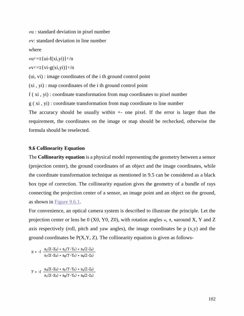
102

u : standard deviation in pixel number

v: standard deviation in line number

where

u = {ui-f(xi,yi)} /n

v = {vi-g(xi,yi)} /n

(ui, vi) : image coordinates of the i th ground control point

(xi , yi) : map coordinates of the i th ground control point

f ( xi , yi) : coordinate transformation from map coordinates to pixel number

g ( xi , yi) : coordinate transformation from map coordinate to line number

The accuracy should be usually within +- one pixel. If the error is larger than the

requirement, the coordinates on the image or map should be rechecked, otherwise the

formula should be reselected.

9.6 Collinearity Equation

The Collinearity equation is a physical model representing the geometry between a sensor

(projection center), the ground coordinates of an object and the image coordinates, while

the coordinate transformation technique as mentioned in 9.5 can be considered as a black

box type of correction. The collinearity equation gives the geometry of a bundle of rays

connecting the projection center of a sensor, an image point and an object on the ground,

as shown in Figure 9.6.1.

For convenience, an optical camera system is described to illustrate the principle. Let the

projection center or lens be 0 (X0, Y0, Z0), with rotation angles , , around X, Y and Z

axis respectively (roll, pitch and yaw angles), the image coordinates be p (x,y) and the

ground coordinates be P(X,Y, Z). The collinearity equation is given as follows-

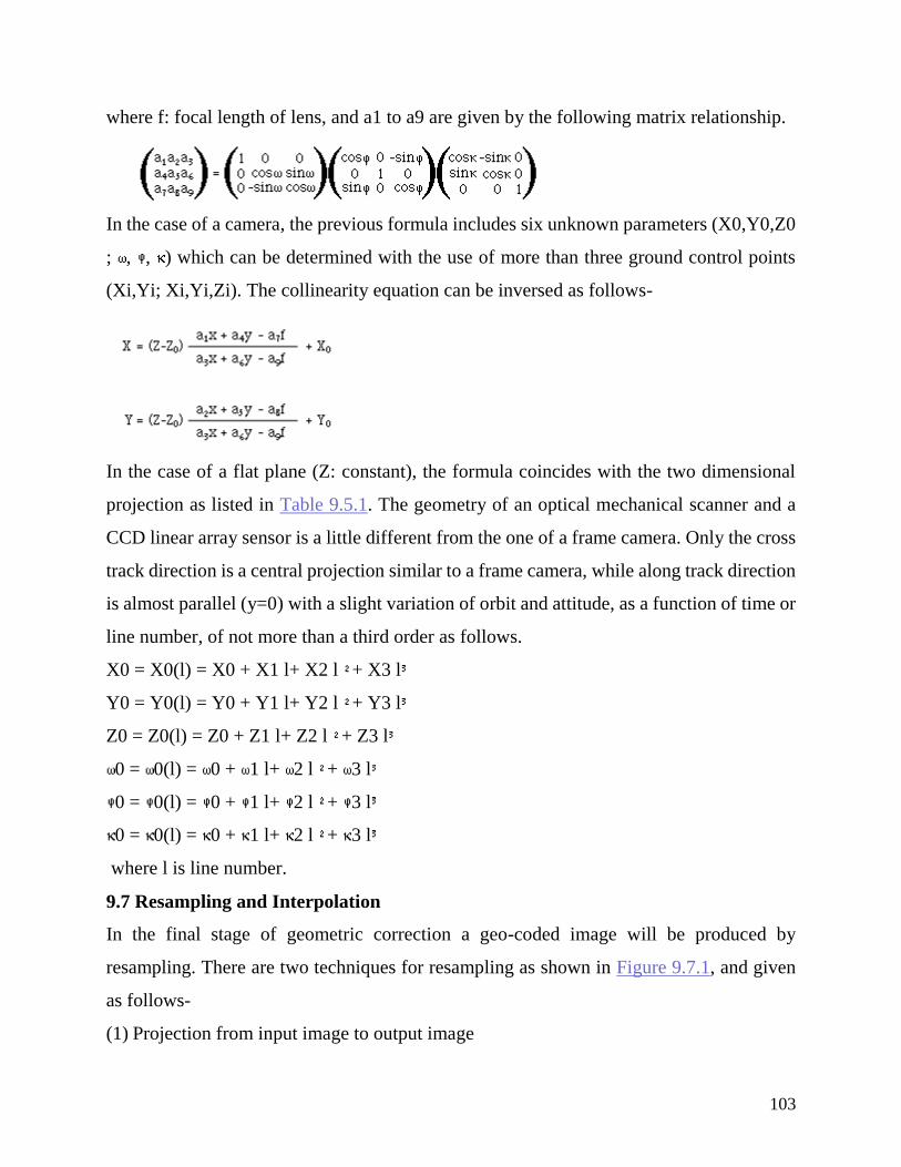
103

where f: focal length of lens, and a1 to a9 are given by the following matrix relationship.

In the case of a camera, the previous formula includes six unknown parameters (X0,Y0,Z0

; , , ) which can be determined with the use of more than three ground control points

(Xi,Yi; Xi,Yi,Zi). The collinearity equation can be inversed as follows-

In the case of a flat plane (Z: constant), the formula coincides with the two dimensional

projection as listed in Table 9.5.1. The geometry of an optical mechanical scanner and a

CCD linear array sensor is a little different from the one of a frame camera. Only the cross

track direction is a central projection similar to a frame camera, while along track direction

is almost parallel (y=0) with a slight variation of orbit and attitude, as a function of time or

line number, of not more than a third order as follows.

X0 = X0(l) = X0 + X1 l+ X2 l + X3 l

Y0 = Y0(l) = Y0 + Y1 l+ Y2 l + Y3 l

Z0 = Z0(l) = Z0 + Z1 l+ Z2 l + Z3 l

0 = 0(l) = 0 + 1 l+ 2 l + 3 l

0 = 0(l) = 0 + 1 l+ 2 l + 3 l

0 = 0(l) = 0 + 1 l+ 2 l + 3 l

where l is line number.

9.7 Resampling and Interpolation

In the final stage of geometric correction a geo-coded image will be produced by

resampling. There are two techniques for resampling as shown in Figure 9.7.1, and given

as follows-

(1) Projection from input image to output image

104

Each pixel of the input image is projected to the output image plane. In this case, an image

output device with random access such as flying spot scanner is required.

(2) Projection from output image to input image

Regularly spaced pixels in the output image plane are projected into the input image plane

and their values interpolated from the surrounding input image data. This is a more general

method.

Usually the inverse equation to transform from the output image coordinate system to the

input image coordinate system, is not possible to determine because the geometric equation

is very complex. In such a case, the following methods can be adopted-

(1) Partition into small areas

As a small area can be approximated by the lower order polynomials, such as affine or

pseudo affine transformation, the inverse equation can be easily determined. Resampling

can be undertaken for each small area, one by one.

(2) Line and pixel functions

A line function can be determined approximately to search for a scan line number which is

closest to the pixel to be resampled, while a pixel function can be determined to search for

the pixel number.

In resampling as shown in Figure 9.7.1(b), a projected point in an input image plane does

not coincide with the input image data. Therefore the spectral data should be interpolated,

and the following methods can be used-

(1) Nearest neighbor (NN)

As shown in Figure 9.7.2 (a), the nearest point will be sampled. The geometric error will

be a half pixel at maximum. It has the advantage of being easy and fast.

(2) Bi-linear (BL)

As shown in Figure 9.7.2 (b), the bi-linear function is applied to the surrounding four

points. The spectral data will be smoothed after the interpolation.

(3) Cubic convolution (CC)

As shown in Figure 9.7.2 (c), the spectral data will be interpolated by a cubic function

using the surrounding sixteen points.The cubic convolution results in sharpening as well

105

as smoothing, though the computation takes a longer time when compared with the other

methods

9.8 Map Projection

A map projection is used project the rotated ellipse representing the earth's shape, to a

two-dimensional plane. However there will remain some distortions because the curved

surface of the earth cannot be projected precisely on to a plane.

There are three major map projection techniques; perspective projection, conical projection

and cylindrical projection, which are used in remote sensing. There are described as

follows.

a. Perspective projection

The perspective projection projects the earth from a projection center to a plane as shown

in Figure 9.8.1. The Polar stereo projection is a perspective projection, as shown in Figure

9.8.2, which projects the northern or southern hemisphere from a projection center at the

opposite pole to a vertical plane tangent at the pole. The NOAA Global Vegetation Index

(GVI) data are edited in the polar stereo projection.

b. Conical projection

The conical projection projects the earth from the center of the earth to a conical body

which envelops the earth. The Lambertian conical projection is a typical conical

projection with the axis of the conical body identical to the axis of the earth. Aerial

navigation charts are drawn using this projection for mid-latitudes, with wider areas from

the west to the east.

c. Cylindrical projection

The cylindrical projection projects the earth from the center of the earth to a cylinder which

envelops or intersects the earth. The Mercator projection, as shown in Figure 9.8.3, is a

typical cylindrical projection with the equator tangent to the cylinder. The Universal

Transverse Mercator (UTM) is also an internationally popular map projection. UTM is

a type of Gauss-Kruger projection, with the meridian tangent to the cylinder, as shown

in Figure 9.8.4. The UTM has an origin point at every six degrees of longitude with a scale

106

factor of 0.9996 at the origin and 1.0000 at a distance of 90 kilometers from the central

meridian.

d. Other projections

For computer processing, a grid coordinate system with equal intervals of latitude and

longitude, is often more convenient.

Chapter 10 Image Processing –

Conversion

10.1 Image Enhancement and Feature Extraction

Image enhancement can be defined as conversion of the image quality to a better and

more understandable level for feature extraction or image interpretation, while radiometric

correction is to reconstruct the physically calibrated value from the observed data.

On the other hand, feature extraction can be defined as the operation to quantify the image

quality through various parameters or functions, which are applied to the original image.

These processes can be considered as conversion of the image data. Image enhancement is

applied mainly for image interpretation in the form of an image output, while feature

extraction is normally used for automated classification or analysis in a quantitative form

(see Figure 10.1.1).

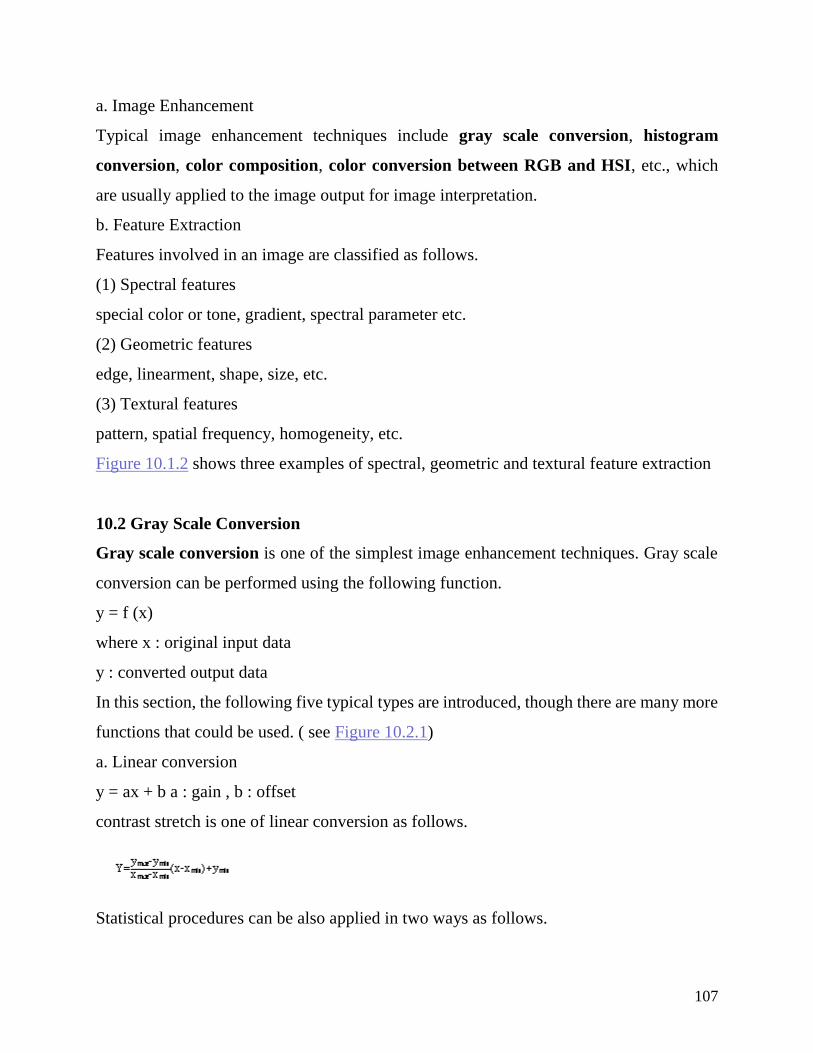
107

a. Image Enhancement

Typical image enhancement techniques include gray scale conversion, histogram

conversion, color composition, color conversion between RGB and HSI, etc., which

are usually applied to the image output for image interpretation.

b. Feature Extraction

Features involved in an image are classified as follows.

(1) Spectral features

special color or tone, gradient, spectral parameter etc.

(2) Geometric features

edge, linearment, shape, size, etc.

(3) Textural features

pattern, spatial frequency, homogeneity, etc.

Figure 10.1.2 shows three examples of spectral, geometric and textural feature extraction

10.2 Gray Scale Conversion

Gray scale conversion is one of the simplest image enhancement techniques. Gray scale

conversion can be performed using the following function.

y = f (x)

where x : original input data

y : converted output data

In this section, the following five typical types are introduced, though there are many more

functions that could be used. ( see Figure 10.2.1)

a. Linear conversion

y = ax + b a : gain , b : offset

contrast stretch is one of linear conversion as follows.

Statistical procedures can be also applied in two ways as follows.

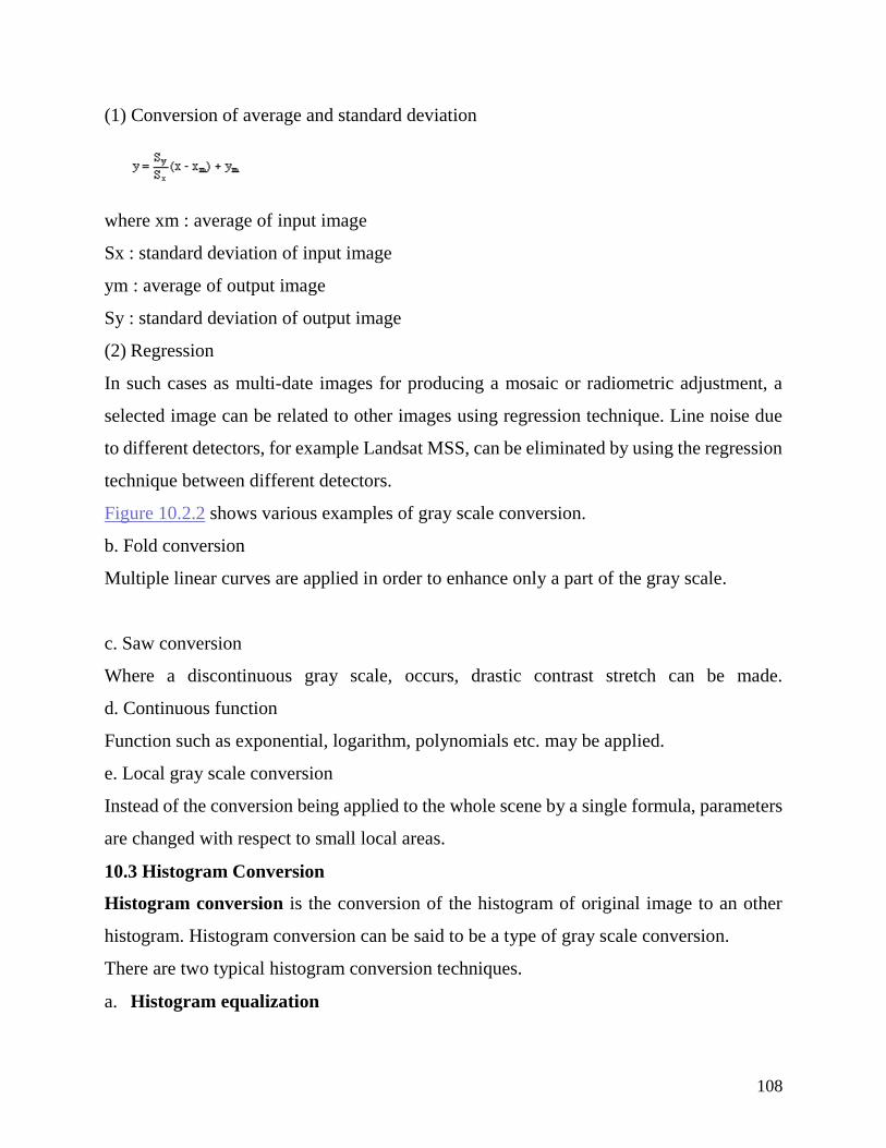
108

(1) Conversion of average and standard deviation

where xm : average of input image

Sx : standard deviation of input image

ym : average of output image

Sy : standard deviation of output image

(2) Regression

In such cases as multi-date images for producing a mosaic or radiometric adjustment, a

selected image can be related to other images using regression technique. Line noise due

to different detectors, for example Landsat MSS, can be eliminated by using the regression

technique between different detectors.

Figure 10.2.2 shows various examples of gray scale conversion.

b. Fold conversion

Multiple linear curves are applied in order to enhance only a part of the gray scale.

c. Saw conversion

Where a discontinuous gray scale, occurs, drastic contrast stretch can be made.

d. Continuous function

Function such as exponential, logarithm, polynomials etc. may be applied.

e. Local gray scale conversion

Instead of the conversion being applied to the whole scene by a single formula, parameters

are changed with respect to small local areas.

10.3 Histogram Conversion

Histogram conversion is the conversion of the histogram of original image to an other

histogram. Histogram conversion can be said to be a type of gray scale conversion.

There are two typical histogram conversion techniques.

a. Histogram equalization

109

b. Histogram equalization is to convert the histogram of an original image to equalized

histogram as shown in Figure 10.3.1. As a first step, an accumulated histogram should be

made. Then the accumulated histogram should be divided into a number of equal regions.

Thirdly , the corresponding gray scale in each region should be assigned to a converted

gray scale.

The effect of histogram equalization is that parts of the image with more frequency

variation will be more enhanced, while parts of an image with less frequency will be

neglected.

Figure 10.3.2 shows a comparison between the original image and the converted image,

after histogram equalization.

c. Histogram normalization

Generally a normal distribution of the density in an image would create an image that is

natural for a human observation. In this sense the histogram of the original image may be

sometimes converted to the normalized histogram. However in this conversion, pixels with

same gray scale should be reallocated to other pixels with a different gray scales, in order

to form a normalized histogram.

Therefore such a gray scale conversion is not a 1:1 conversion and thus enables no reverse

conversion. Histogram normalization may be applied, for example, to an unfocused image

of a planet with a low dynamic range, though it is not be very much popular for ordinary

remote sensing data

10.4 Color Display of Image Data

Color display of remote sensing data is of importance for effective visual interpretation.

There are two color display methods; color composite, to generate color with multi-band

data and pseudo-color display, to assign different colors to the gray scale of a single image.

a. Color Composite

A color image can be generated by composing three selected multi-band images with the

use of three primary colors. Different color images may be obtained depending on the

selection of three band images and the assignment of the three primary colors.

110

There are two methods of color composite; an additive color composite and a subtractive

color composite, as shown in Figure 10.4.1. Additive color composite uses three light

sources of three primary colors (Blue, Green and Red) for example, in a multispectral

viewer or color graphic display. The subtractive color composite, uses three pigments of

three primary color (Cyan, Magenta and Yellow), for example, in color printing.

When three filters of B, G and R are assigned to the same spectral regions of blue, green

and red as shown in Figure 10.4.2, almost the same color as the natural scale, can be

reproduced, and is called a natural color composite.

However in remote sensing multi-band images are not always divided in to the same

spectral regions as the three primary color filters. In addition invisible regions, such as

infrared, are often used, which are required to be displayed in color. As a color composite

with an infrared band is no longer natural color, it is called a false color composite.

In particularly the color composite with the assignment of blue to the green band, green to

the red band and red to the near infrared band is very popular, and is called an infrared

color composite, which is the same as found in color infrared film (see Figure 10.4.2).

In the case of digital data, three values corresponding to R, G and B will make various

color combinations, as listed in Table 10.4.1.

b. Pseudo Color Display

Different colors may be assigned to the subdivided gray scale of a single image. Such a

color allocation is called pseudo-color. For example, a pseudo-color image of a thermal

infrared image will give a temperature map. If one wishes to produce a continuous color

tone, three different functions of three primary colors should be applied. Figure 10.4.3 is

an example of a pseudo-color display with continuous color tone.

10.5 Color Representation - Color Mixing System

Light is perceived as color by the human eye, termed color stimulus, and corresponds to

the visible region of electro-magnetic spectrum, with a specific spectral curve of radiance

as shown in Figure 10.5.1.

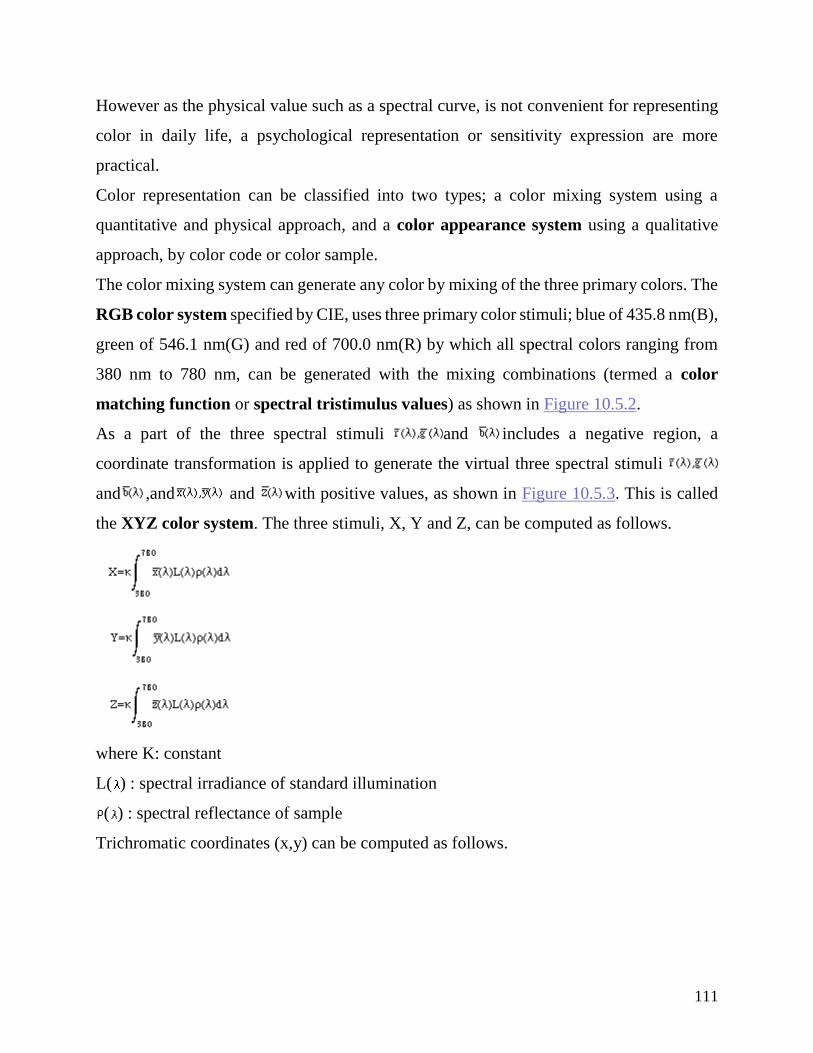
111

However as the physical value such as a spectral curve, is not convenient for representing

color in daily life, a psychological representation or sensitivity expression are more

practical.

Color representation can be classified into two types; a color mixing system using a

quantitative and physical approach, and a color appearance system using a qualitative

approach, by color code or color sample.

The color mixing system can generate any color by mixing of the three primary colors. The

RGB color system specified by CIE, uses three primary color stimuli; blue of 435.8 nm(B),

green of 546.1 nm(G) and red of 700.0 nm(R) by which all spectral colors ranging from

380 nm to 780 nm, can be generated with the mixing combinations (termed a color

matching function or spectral tristimulus values) as shown in Figure 10.5.2.

As a part of the three spectral stimuli and includes a negative region, a

coordinate transformation is applied to generate the virtual three spectral stimuli

and ,and and with positive values, as shown in Figure 10.5.3. This is called

the XYZ color system. The three stimuli, X, Y and Z, can be computed as follows.

where K: constant

L( ) : spectral irradiance of standard illumination

( ) : spectral reflectance of sample

Trichromatic coordinates (x,y) can be computed as follows.

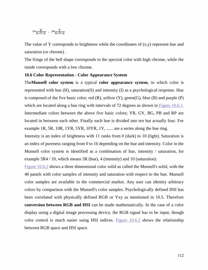
112

The value of Y corresponds to brightness while the coordinates of (x,y) represent hue and

saturation (or chrome) .

The fringe of the bell shape corresponds to the spectral color with high chrome, while the

inside corresponds with a low chrome.

10.6 Color Representation - Color Appearance System

TheMunsell color system is a typical color appearance system, in which color is

represented with hue (H), saturation(S) and intensity (I) as a psychological response. Hue

is composed of the five basic color; red (R), yellow (Y), green(G), blue (B) and purple (P)

which are located along a hue ring with intervals of 72 degrees as shown in Figure 10.6.1.

Intermediate colors between the above five basic colors; YR, GY, BG, PB and RP are

located in between each other. Finally each hue is divided into ten but actually four. For

example 1R, 5R, 10R, 1YR, 5YR, 10YR, 1Y, ...... are a series along the hue ring.

Intensity is an index of brightness with 11 ranks from 0 (dark) to 10 (light). Saturation is

an index of pureness ranging from 0 to 16 depending on the hue and intensity. Color in the

Munsell color system is identified as a combination of hue, intensity / saturation, for

example 5R4 / 10, which means 5R (hue), 4 (intensity) and 10 (saturation).

Figure 10.6.2 shows a three dimensional color solid as called the Munsell's solid, with the

40 panels with color samples of intensity and saturation with respect to the hue. Munsell

color samples are available in the commercial market. Any user can identity arbitrary

colors by comparison with the Munsell's color samples. Psychologically defined HSI has

been correlated with physically defined RGB or Yxy as mentioned in 10.5. Therefore

conversion between RGB and HSI can be made mathematically. In the case of a color

display using a digital image processing device, the RGB signal has to be input, though

color control is much easier using HSI indices. Figure 10.6.3 shows the relationship

between RGB space and HSI space.

113

The following are conversions from RGB to HSI, and from HSI to RGB. The ranges of

R,G,B,S,I are [0,1] :, the range of H is [0,2p].

(1) from RGB to HIS

I = Max. (R,G,B)

1) I = 0 ; S = 0, H= indeterminate

S = (I-i)/I , where i = min. {R, G, B}

Let r = (I-R) / (I-i), g = (I-G) / (I-i), b = (I-B) / (I-i), then

if R = I H = (b-g) / 3

if G = I H = (2+r-b) / 3

if B = I H = (4+g-r) / 3

(2) from HSI to RGB

1) S = 0 ; R = G = B = I regardless of value of H

H' = 3H / h = floor(H') If H = 2 , then H = 0

(floor (x): the function of getting the truncated value of x)

P = I(1-S), Q = I{1-S (H' - h)} , T = I {1-S(1-H'+h)} , then

h = 0 R = I, G = T, B = P

h = 1 R = Q, G = I, B = P

h = 2 R = P, G = I, B = T

h = 3 R = P, G = Q, B = I

h = 4 R = I, G = P, B = Q

h = 5 R = I, G = P, B = Q

10.7 Operations between Images

Operations between multi-spectral images or multi-date images are very useful for image

enhancement and feature extraction.

Operations between images include two techniques; arithmetic operation and logical

operation.

a. Arithmetic Operations

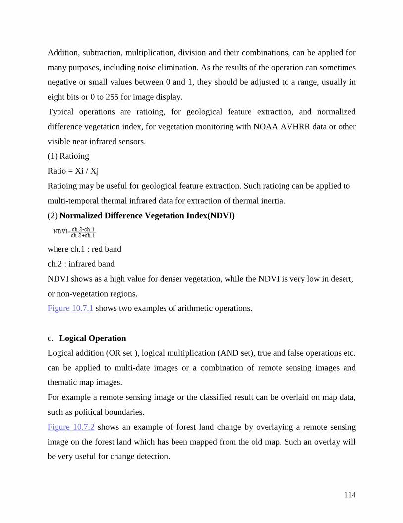
114

Addition, subtraction, multiplication, division and their combinations, can be applied for

many purposes, including noise elimination. As the results of the operation can sometimes

negative or small values between 0 and 1, they should be adjusted to a range, usually in

eight bits or 0 to 255 for image display.

Typical operations are ratioing, for geological feature extraction, and normalized

difference vegetation index, for vegetation monitoring with NOAA AVHRR data or other

visible near infrared sensors.

(1) Ratioing

Ratio = Xi / Xj

Ratioing may be useful for geological feature extraction. Such ratioing can be applied to

multi-temporal thermal infrared data for extraction of thermal inertia.

(2) Normalized Difference Vegetation Index(NDVI)

where ch.1 : red band

ch.2 : infrared band

NDVI shows as a high value for denser vegetation, while the NDVI is very low in desert,

or non-vegetation regions.

Figure 10.7.1 shows two examples of arithmetic operations.

c. Logical Operation

Logical addition (OR set ), logical multiplication (AND set), true and false operations etc.

can be applied to multi-date images or a combination of remote sensing images and

thematic map images.

For example a remote sensing image or the classified result can be overlaid on map data,

such as political boundaries.

Figure 10.7.2 shows an example of forest land change by overlaying a remote sensing

image on the forest land which has been mapped from the old map. Such an overlay will

be very useful for change detection.

115

10.8 Principal Component Analysis

Principal component analysis is used to reduce the dimensions of measured variables (p

dimension) to the representative principal components (m dimension , m

Let the measured p dimensional variables be {xi } i = 1,p, the principal components{zk }

k = 1, m can be expressed as the linear combination as follows.

zk = a1k x1 + a2k x2 + ...... + apk xp

The coefficients (a1k - apk ) are determined under the following constrains.

(1) aik = 1

(2) Variance zk should be maximum

(3) zk and z k+1 should be independent of each other

The solution of the above problem can be obtained by determining the unique values and

the unique vectors which correspond to the variance and vector of the principal components

respectively.

The unique value represents the contribution ratio which indicates how much percentage

the principal component represents of the total tendency of the variables. The

accumulative contribution ratio percentage all the principal components represent of the

total tendency of the variables. Using an accumulative contribution ratio of 80 - 90 percent,

will indicate how many principal components should be adopted to effectively represent

the major variations in the image data.

Graphically speaking, the first principal component for example in the case of two

dimensional variables (see Figure 10.8.1) will be the principal axis which gives the

maximum variance. The principal component analysis can be used for the following

applications.

(1) Effective classification of land use with multi-band data

(2) Color representation or visual interpretation with multi-band data

(3) Change detection with multi-temporal data

In the case of multi-band data with more than four bands, all bands cannot be assigned to

R, G or B at the same time. However the first three principal components can represent up

to five spectral variables with little information loss.

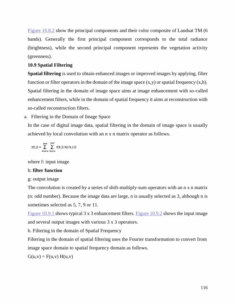
116

Figure 10.8.2 show the principal components and their color composite of Landsat TM (6

bands). Generally the first principal component corresponds to the total radiance

(brightness), while the second principal component represents the vegetation activity

(greenness).

10.9 Spatial Filtering

Spatial filtering is used to obtain enhanced images or improved images by applying, filter

function or filter operators in the domain of the image space (x,y) or spatial frequency (x,h).

Spatial filtering in the domain of image space aims at image enhancement with so-called

enhancement filters, while in the domain of spatial frequency it aims at reconstruction with

so-called reconstruction filters.

a. Filtering in the Domain of Image Space

In the case of digital image data, spatial filtering in the domain of image space is usually

achieved by local convolution with an n x n matrix operator as follows.

where f: input image

h: filter function

g: output image

The convolution is created by a series of shift-multiply-sum operators with an n x n matrix

(n: odd number). Because the image data are large, n is usually selected as 3, although n is

sometimes selected as 5, 7, 9 or 11.

Figure 10.9.1 shows typical 3 x 3 enhancement filters. Figure 10.9.2 shows the input image

and several output images with various 3 x 3 operators.

b. Filtering in the domain of Spatial Frequency

Filtering in the domain of spatial filtering uses the Fourier transformation to convert from

image space domain to spatial frequency domain as follows.

G(u,v) = F(u,v) H(u,v)

117

F: Fourier transformation of input image

H: filter function

An output image from filtering of spatial frequency, can be obtained by using an inverse

Fourier transformation of the above formula.

Low pass filters, high pass filters, band pass filters etc., are typical filters with a criterion

of frequency control. Low pass filters which out puts only lower frequency image data, less

than a specified threshold, can be applied to remove high frequency, noise,while high pass

filter are used for removing, for example, stripe noise of low frequency.

10.10 Texture Analysis

Texture is a combination of repeated patterns with a regular frequency. In visual

interpretation texture has several types, for example, smooth, fine, coarse etc., which are

often used in the classification of forest types. Texture analysis is defined as the

classification or segmentation of textural features with respect to the shape of a small

element, density and direction of regularity.

Figure 10.10.1 (a) shows two different textures of density, while Figure 10.10.1 (b) shows

two different textures with respect to the shape of the elements.

In the case of digital image, it is difficult to treat the texture mathematically because texture

cannot be standardized quantitatively and the data volume is so huge.

However texture analysis has been made with statistical features which are combined with

spectral data for improving land cover classification. Power spectrum analysis is another

form of textural analysis in which direction and wavelength or frequency can be determined

for regular patterns of , for example, sea waves and sand waves in the desert.

a. Use of Statistical Features

The following statistical values of an n x n window can be used as textural information

(1) Gray level histogram

(2) Variance - co-variance matrix

(3) Run-length matrix

These values are used for classification together with the spectral data.Figure 10.10.2 (a)

shows the land cover classification using only spectral data while Figure 10.10.2 (b) shows

118

the result of classification with spectral data as well as textural information. The result

shows a better classification for the urban area which has a higher frequency and variance

of image density.

b. Analysis using Power Spectrum

Power spectrum analysis is useful for those images which have regular wave patterns with

a constant interval, such as glitter image of the sea surface or wave patterns of sand dunes.

Fourier transformation is applied to determine the power spectrum which gives the

frequency and direction of the pattern.

10.11 Image Correlation

Image correlation is a technique by which the conjugate point of a slave image (right)

corresponding to the master image (left) will be searched for the maximum correlation

coefficient. Image correlation is applied to stereo images for DEM (digital elevation model)

generation or multi-date images for automated recognition of ground control points.

As shown in Figure 10.11.1, the master window in the left image is fixed, while the slave

window in the right image is moved to search for the maximum image correlation as

computed from the following formula.

or

where ai : image data of the master window

bi : image data of the slave window

n : total number of image data

Because the above two correlations show almost no difference, the first correlation is

preferred to save computing time.

119

The size of the window should be selected depending on the image resolution and feature

size. For example, 5 x 5 to 9 x 9 windows might be selected for SPOT stereo images, while

9 x 9 to 21 x 21 would be better used for digitized aerial photographs.

When the conjugate points of stereo images are determined, the corresponding digital

elevation can be computed using collinearity equations based on photogrammetric theory.

Figure 10.11.2 shows the conjugate points as white dots in a pair of SPOT stereo images,

which were automatically recognized by image correlation techniques.

Chapter 11 Image Processing –

Classification

11.1 Classification Techniques

Classification of remotely sensed data is used to assign corresponding levels with respect

to groups with homogeneous characteristics, with the aim of discriminating multiple

objects from each other within the image.

120

The level is called class. Classification will be executed on the base of spectral or spectrally

defined features, such as density, texture etc. in the feature space. It can be said that

classification divides the feature space into several classes based on a decision rule. Figure

11.1.1 shows the concept of classification of remotely sensed data

. In many cases, classification will be undertaken using a computer, with the use of

mathematical classification techniques. Classification will be made according to the

following procedures as shown in Figure 11.1.2.

Step 1: Definition of Classification Classes

Depending on the objective and the characteristics of the image data, the classification

classes should be clearly defined.

Step 2: Selection of Features

Features to discriminate between the classes should be established using multi-spectral

and/or multi-temporal characteristics, textures etc.

Step 3: Sampling of Training Data

Training data should be sampled in order to determine appropriate decision rules.

Classification techniques such as supervised or unsupervised learning will then be selected

on the basis of the training data sets.

Step 4: Estimation of Universal Statistics

Various classification techniques will be compared with the training data, so that an

appropriate decision rule is selected for subsequent classification.

Step 5: Classification

Depending up on the decision rule, all pixels are classified in a single class. There are two

methods of pixel by pixel classification and per-field classification, with respect to

segmented areas.

Popular techniques are as follows.

a. Multi-level slice classifier

b. Minimum distance classifier

c. Maximum likelihood classifier

d. Other classifiers such as fuzzy set theory and expert systems

121

Step 6: Verification of Results

The classified results should be checked and verified for their accuracy and reliability.

11.2 Estimation of Population Statistics

a. Supervised classification

In order to determine a decision rule for classification, it is necessary to know the spectral

characteristics or features with respect to the population of each class. The spectral features

can be measured using ground-based spectrometers. However due to atmospheric effects,

direct use of spectral features measured on the ground are not always available. For this

reason, sampling of training data from clearly identified training areas, corresponding to

defined classes is usually made for estimating the population statistics (see Figure 11.2.1).

This is called supervised classification. Statistically unbiased sampling of training data

should be made in order to represent the population correctly.

b. Unsupervised Classification

In the case where there is less information in an area to be classified, only the image

characteristics are used as follows.

(1) Multiple groups, from randomly sampled data, will be mechanically divided into

homogeneous spectral classes using a clustering technique (see 11.3).

(2) The clustered classes are then used for estimating the population statistics. This

classification technique is called unsupervised classification (see Figure 11.2.2).

c. Estimation of Population Statistics

Maximum likelihood estimation is the most popular method by which the population

statistics such as mean and variance, are estimated to maximize the probability or

likelihood from a defined probability density function within the feature space.

In most cases, the probability density function is selected to be a multiple normal

distribution. The multiple normal distribution gives the following the maximum likelihood

estimator.

122

Variance - covariance matrix

where m: number of bands

n: number of pixels

Before adopting the maximum likelihood classification, it should be checked to determine

if the distribution of training data will fit the normal distribution or not.

11.3 Clustering

Clustering is a grouping of data with similar characteristics. Clustering is divided into

hierarchical clustering and non-hierarchical clustering as mentioned as follows.

a. Hierarchical Clustering

b. The similarity of a cluster is evaluated using a "distance" measure. The minimum

distance between clusters will give a merged cluster after repeated procedures from a

starting point of pixel-wise clusters to a final limited number of clusters.

Figure 11.3.1 shows the general procedure of hierarchical clustering.

The distances to evaluate the similarity are selected from the following methods.

(1) Nearest neighbor method

Nearest neighbor with minimum distance will form a new merged cluster.

(2) Furthest neighbor method

Furthest neighbor with maximum distance will form a new merged cluster.

(3) Centroid method

Distance between the gravity centers of two clusters is evaluated for merging a new

merged cluster.

(4) Group average method

Root mean square distance between all pairs of data within two different clusters, is used

for clustering.

(5) Ward method

Root mean square distance between the gravity center and each member is minimized.

b. Non-hierarchical Clustering

123

At the initial stage, an arbitrary number of clusters should be temporally chosen. The

members belonging to each cluster will be checked by selected parameters or distance and

relocated into the more appropriate clusters with higher separability. The ISODATA

method and K-mean method are examples of non-hierarchical clustering.

The ISODATA method is composed of the following procedures (see Figure 11.3.2).

(1) All members are relocated into the closest clusters by computing the distance between

the member and the clusters.

(2) The center of gravity of all clusters is recalculated and the above procedure is repeated

until convergence.

(3) If the number of clusters is within a certain specified number, and the distances between

the clusters meet a prescribed threshold, the clustering is considered complete.

11.4 Parallelpiped Classifier

The parallelpiped classifier (often termed multi-level slicing) divides each axis of multi-

spectral feature space, as shown in an example in Figure 11.4.1. The decision region for

each class is defined on the basis of a lowest and highest value on each axis. The accuracy

of classification depends on the selection of the lowest and highest values in consideration

of the population statistics of each class. In this respect, it is most important that the

distribution of population of each class is well understood.

The parallelpiped classifier is very simple and easy to understand schematically. In addition

the computing time will be a minimum, when compared with other classifiers.

However the accuracy will be low especially when the distribution in feature space has

covariance or dependency with oblique axes. Orthogonalization should be undertaken

using principal component analysis, for example, before adopting the parallelpiped

classifier.

Figure 11.4.2 shows an example of classification with the use of the parallelpiped classifier

11.5 Decision Tree Classifier

The decision tree classifier is an hierarchically based classifier which compares the data

with a range of properly selected features. The selection of features is determined from an

assessment of the spectral distributions or separability of the classes. There is no generally

124

established procedure. Therefore each decision tree or set of rules should be designed by

an expert. When a decision tree provides only two outcomes at each stage, the classifier is

called a binary decision tree classifier (BDT).

Figure 11.5.1 shows the spectral characteristics of ground truth data for nine classes and

the corresponding decision tree classifier to classify the nine classes using their spectral

characteristics.

Generally a group of classes will be classified into two groups with the highest separability

with respect to a feature.

Features often used are as follows.

(1) Spectral values

(2) An index which is computed from spectral values. For example, the vegetation index

is a popular indices.

(3) any arithmetic value such as addition, subtraction or ratioing.

(4) Principal components.

The advantages of the decision tree classifier are that computing time is less than the

maximum likelihood classifier and by comparison the statistical errors are avoided.

However the disadvantage is that the accuracy depends fully on the design of the decision

tree and the selected features.

Figure 11.5.2 shows an example of classification with a decision tree classifier.

11.6 Minimum Distance Classifier

The minimum distance classifier is used to classify unknown image data to classes which

minimize the distance between the image data and the class in multi-feature space. The

distance is defined as an index of similarity so that the minimum distance is identical to the

maximum similarity. Figure 11.6.1 shows the concept of a minimum distance classifier.

The following distances are often used in this procedure.

(1) Euclidian distance

125

Is used in cases where the variances of the population classes are different to each other.

The Euclidian distance is theoretically identical to the similarity index.

(2) Normalized Euclidian distance

The Normalized Euclidian distance is proportional to the similarity in dex, as shown in

Figure 11.6.2, in the case of difference variance.

(3) Mahalanobis distance

(4) In cases where there is correlation between the axes in feature space, the Mahalanobis

distance with variance-covariance matrix, should be used as shown in Figure 11.6.3.

where X : vector of image data (n bands)

X = [ x1, x2, .... xn]

k : mean of the kth class

k = [ m1, m2, .... mn]

k : variance matrix

k : variance-covariance matrix

Figure 11.6.4 shows examples of classification with the three distances.

11.7 Maximum Likelihood Classifier

The maximum likelihood classifier is one of the most popular methods of classification

in remote sensing, in which a pixel with the maximum likelihood is classified into the

126

corresponding class. The likelihood Lk is defined as the posterior probability of a pixel

belonging to class k.

Lk = P(k/X) = P(k)*P(X/k) / P(i)*P(X/i)

where P(k) : prior probability of class k

P(X/k) : conditional probability to observe X from class k, or probability density function

Usually P(k) are assumed to be equal to each other and P(i)*P(X/i) is also common to all

classes. Therefore Lk depends on P(X/k) or the probability density function.

For mathematical reasons, a multivariate normal distribution is applied as the probability

density function. In the case of normal distributions, the likelihood can be expressed as

follows.

where n: number of bands

X: image data of n bands

Lk(X) : likelihood of X belonging to class k

k : mean vector of class k

k : variance-covariance matrix of class k

In the case where the variance-covariance matrix is symmetric, the likelihood is the same

as the Euclidian distance, while in case where the determinants are equal each other, the

likelihood becomes the same as the Mahalanobis distances. Figure 11.7.1 shows the

concept of the maximum likelihood method.

The maximum likelihood method has an advantage from the view point of probability

theory, but care must be taken with respect to the following items.

(1) Sufficient ground truth data should be sampled to allow estimation of the mean

vector and the variance-covariance matrix of population.

(2) The inverse matrix of the variance-covariance matrix becomes unstable in the case

where there exists very high correlation between two bands or the ground truth data are

127

very homogeneous. In such cases, the number of bands should be reduced by a principal

component analysis.

(3) When the distribution of the population does not follow the normal distribution, the

maximum likelihood method cannot be applied.

Figure 11.7.2 shows an example of classification by the maximum likelihood method.

11.8 Applications of Fuzzy Set Theory

Fuzzy set theory, to treat fuzziness in data, was proposed by Zadeh in 1965. In Fuzzy set

theory the membership grade can be taken as a value intermediate between 0 and 1 although

in the normal case of set theory membership the grade can be taken only as 0 or 1.

Figure 11.8.1 shows a comparison between the normal case of set theory and fuzzy set

theory. The function of the membership grade is called its "membership function" in Fuzzy

theory. The membership function will be defined by the user in consideration of the

fuzziness.

In remote sensing it is often not easy to delineate the boundary between two different

classes. For example, there are transitive vegetation or mixed vegetation between forest

and grass land. In such cases as unclearly defined class boundaries, Fuzzy set theory can

be usefully applied, in a qualitative sense.

The following shows how the maximum likelihood method with Fuzzy set theory. Let the

membership function be Mf( ) of class k (k=1,n), the likelihood Lf of fuzzy class f can be

defined as follows.

Fuzzy set theory can be also extended to clustering. Figure 11.8.2 shows an example of

land cover classification using Fuzzy set theory. In this classification, the concrete structure

(code 90), with clearly defined characteristics, was first classified using the ordinary

maximum likelihood method, while the loosely defined urban classes were classified by

the fuzzy based maximum likelihood method.

11.9 Classification using an Expert System

128

Experts interpret remote sensing images with knowledge based on experience. However

computer assisted classification utilizes only very limited expert knowledge. The expert

system, therefore, is a problem solving system which supports expert knowledge in a

computer based system.

The following two types of knowledge are required for an expert system in remote sensing.

(1) Knowledge about image analysis

Procedures for image analysis can be made only with adequate knowledge about image

processing and analysis. A feedback system should be introduced for checking and

evaluating the objectives and the results.

(3) Knowledge about the objects to be analyzed

Knowledge about the objects to be recognized or classified should be introduced in addition

to the ordinary classification method. The fact that forest does not exist over 3,000 meters

above sea level, is one example of the type of knowledge that can be introduced.

Table 11.9.1 shows a list of knowledge required for delineating a tidal front in sea surface

condition mapping. Figure 11.9.1 shows the sea surface condition map that was interpreted

by an expert. Such knowledge will assure an increase in the accuracy or reliability of

classification.

In many cases, knowledge can be represented as "if A is ..., then B becomes...." which is

called the IF/THEN rule or production rule.

If the IF/THEN rule is fuzzy, then Fuzzy set theory can be also introduced to the expert

system.

Figure 11.9.2 shows an example of the delineation of a tidal front using the expert system.

The expert system can be integrated with a geographic information system (GIS). It is

necessary to accumulate experiences and to evaluate the knowledge for an expert system

to be operationally applied.

129

Chapter 12 Applications of Remote

Sensing

12.1 Land Cover Classification

Land cover mapping is one of the most important and typical applications of remote

sensing data. Land cover corresponds to the physical condition of the ground surface, for

130

example, forest, grassland, concrete pavement etc., while land use reflects human activities

such as the use of the land, for example, industrial zones, residential zones, agricultural

fields etc.

Generally land cover does not coincide with land use. A land use class is composed of

several land covers. Remote sensing data can provide land cover information rather than

land use information.

Initially the land cover classification system should be established, which is usually defined

as levels and classes. The level and class should be designed in consideration of the purpose

of use (national, regional or local), the spatial and spectral resolution of the remote sensing

data, user's request and so on.

The definition should be made as quantitatively clear as possible. Figure 12.1.1 shows an

example of land cover classes for land cover mapping in the Sagami River Basin, Japan,

for use with Landsat MSS data.

The classification was carried out as follows.

a. Geometric correction (see 9.4)

A geo-coded Landsat image was produced.

b. Collection of the ground truth data (see 6.7)

A ground investigation was made to identify each land cover class on the geo-code

Landsat image as well as on topographic maps.

c. Classification by Maximum Likelihood Method (see 11.5 )

The Maximum Likelihood Method was adopted using the training samples obtained from

the ground truth.

Figure 12.1.1 shows the classified land cover map.

Generally Landsat MSS imagery can provide about about ten land cover classes,

depending upon the size and complexity of the classes.

12.2 Land Cover Change Detection

Land cover change detection is necessary for updating land cover maps and the

management of natural resources. The change is usually detected by comparison between

131

two multi-date images, or sometimes between an old map and an updated remote sensing

image.

The method of change detection is divided into two;

a. comparison between two land cover maps which are independently produced

b.change enhancement by integrating two images into a color composite or principal

component image.

Figure 12.2.1 shows the changes over a 5 year period, which were detected by using a color

composite with blue assigned to an old image of Landsat TM and red assigned to a new

image of Landsat TM.

Such detection is very useful for updating "vegetation maps" of 1:50,000 to 1:100,000 scale

with Landsat TM or SPOT, and of 1:250,000 scale with Landsat MSS.

The land cover change can also be divided into two;

a. seasonal change

agricultural lands and deciduous forests change seasonally

b. annual change

land cover or land use changes, which are real changes, for example deforested areas or

newly built towns.

Usually seasonal change and annual change are mixed within the same image. However

only the real change should be detected, so that two multi-data images of almost same

season should be selected to eliminate the effects of seasonal change. One should note that

a cycle of seasonal change can be rather complex as shown in Figure 12.2.2. Sometimes

seasonal change rate is very high, for example in spring time in cold area.

12.3 Global Vegetation Map

NOAA AVHRR data (see 5.1) are very useful for producing a global vegetation maps

which cover the whole world, because NOAA has edited global cloud free mosaics in the

form of a GVI(global vegetation index) on a weekly basis since April of 1982.

132

The GVI data include information about NDVI (normalized difference vegetation index)

as computed as follows

Ch.1 : visible band

Ch.2 : near infrared band

NDVI is sometimes simply called. NVI (normalized vegetation index).

NDVI or NVI are indicators of the intensity of biomass.

The larger the NVI is, the denser the vegetation.

Though the original resolution of NOAA AVHRR is 1.1 km per pixel of the Equator, the

GVI has a low resolution of 16 km x 16 km per pixel at the Equator. In spite of the low

resolution, the GVI is useful for producing a global vegetation map.

As much noise is involved in weekly data, noise free GVI compiled on a monthly base

should be used. Figure 12.3.1 shows six categories out of a total of 13 categories obtained

from cluster analysis (see 11.2).

Figure 12.3.2 shows the result of a cluster analysis applied to GVI data from 1987.

Though the clustered map in Figure 12.3.2 has not yet been verified, it shows the possibility

of using remote sensing data for global map production.

12.4 Water Quality Monitoring

Water pollution has become a very serious problem in big cities and in offshore areas along

industrial zones. Water quality monitoring is one of the typical applications of remote

sensing.

Figure 12.4.1 shows the characteristics of reflection, absorption and scattering on the water

surface, beneath the surface water and from the bottom. The sea color depends on the

absorption and scattering due to water molecules and suspended particles or plankton.

Figure 12.4.2 shows various curves of spectral attenuation with respect to various types of

water. As seen in the figure, clear water has a peak of minimum attenuation around 0.5

m, while turbid water with suspended solid (SS) has larger attenuation with a minimum

peak around 0.55 m. In other word, radiation can penetrate into deep clear water and is

133

scattered by the water volume, causing the typical bluish color. Turbid waters cannot be

penetrated and radiation is scattered near the surface, giving a greenish or yellowish color.

The sea color depends on not only on suspended solids but also the chlorophyll of plankton

within the water body.

Figure 12.4.3 shows an example of the measurement for spectral reflectance of various

amounts of chlorophyll. As seen in the figure, chlorophyll in the sea can be detected in the

region of 0.45 - 0.65 m.

12.5 Measurement of Sea Surface Temperature

Satellite remote sensing can provide thermal information in a short time over a wide area.

Temperature measurement by remote sensing is based on the principle that any object emits

electro-magnetic energy corresponding to the temperature, wavelength and emissivity.

The temperature detected by a thermal sensor is called the "brightness temperature" (see

1.7). Though the brightness temperature coincides with the real temperature if the objects

is a black body, the actual object on the earth has a different emissivity e (e < 1) which

emits electro-magnetic energy of e.I, where I indicates the radiance of a black body with

the same temperature.

Thus the value of e as well as the emitted radiance should be measured in order to compute

the exact temperature, as explained in Figure 12.5.1.

However the value of e for sea water is very nearly equal to 1 and also comparatively

constant, while the value e for ground surfaces is not homogeneous. Thus sea surface

temperature can be estimated more accurately than ground surface temperature.

As the actual brightness temperature includes emitted radiance from the atmosphere, this

will cause a temperature error ranging 2-3 degrees Centigrade between the actual sea

surface temperature and calculated brightness temperature from satellite data. Thus

atmospheric correction (see 9.2) is very important for accurate sea surface temperature

measurement.

Figure 12.5.2 shows the sea surface temperature in pseudo color in Northern Japan using

NOAA AVHRR data which were atmospheric ally as well as geometrically corrected with

overlays of sea coast lines and latitude and longitude grid lines.

134

Using the most recent technology, the estimated accuracy of sea surface temperature is

claimed to be about +-0.5 C on a global scale and about +-0.3 C on a regional scale.

12.6 Snow Survey

As snow cover has a very high reflectance, the aerial distribution of snow can be identified

very easily from satellite remote sensing data. Several models to estimate water resources

in units of snow water equivalent have been proposed with use of the estimated snow

cover area.

Figure 12.6.1 shows a conceptual diagram of the estimation of basin-wide snow water

equivalent with the three parameters of elevation h, latitudinal distribution of snow water

equivalent S(h) and hydrometric curve A(h).

Snow water equivalent Ss in a river basin can be computed as follows.

where hH : maximum elevation

hL: minimum elevation

If snow appears over the average elevation of snow line ho, hL should be replaced by ho.

From the above formula, the latitudinal distribution of snow water equivalent S(h) and the

hydrometric curve A(h) should be determined in order to estimate the snow water

equivalent.

It is known that the snow water equivalent increases linearly proportional to the elevation,

which can ve obtained from the existing snow survey. On the other hand the catchment

area can be expressed in lower order of polynomials as a function of elevation. Therefore

the snow water equivalent can be estimated as a function of percentage of snow cover area

in a river basin.

Figure 12.6.2 shows an estimated curve of snow water equivalent which was obtained from

sample data in the three years of 1979, 1982 and 1983 in the Takaragawa River Basin,

Japan. From the curve, the snow water equivalent can be estimated if the snow cover area

is detected from remote sensing imagery (see a series of examples, Figure 12.6.3(a), (b)

and (c)).

135

Recently microwave remote sensing has been applied to estimate snow volume. Passive

microwave radiometers can provide snow surface temperature with respect to inductivity

of the snow, which may provide snow information. Active microwave radar can provide

reflectivity or scattering of snow with respect to snow density, snow temperature, snow

temperature, size of snow particles etc. It is still difficult to estimate snow volume from

microwave data but several research projects are currently being carried out on this topic.

12.7 Monitoring of Atmospheric Constituents

Each atmospheric constituent such as water vapor, carbon-dioxidide, ozone, methane etc.

has its own unique spectral characteristic of emission and absorption. With the use of these

characteristics, the density of these atmospheric molecules can be monitored by measuring

the spectral energy which transmits from the sun, the moon or the stars through the

atmosphere, the scattering energy from the atmosphere or the clouds, the reflected energy

from the earth surface and/or the thermal radiation emitted from the atmosphere and the

earth surface. The spectral energy can be measured by two methods; absorption

spectroscopy and emission spectroscopy.

These methods have been applied for many years ago for the measurement of the upper

atmosphere from the ground. Recently the methods have been extended for measurements

from aircraft, balloon and satellite. In addition, multi-spectral laser with variable

wavelength, called laser rader or lidar, has been developed for the measurement of the

spatial distribution of the atmospheric constituents.

Figure 12.7.1 shows the spectral transmittance of H2O, CO2, O3, N2O and CH4 in the

infrared region.

Figure 12.7.2 shows the spectral attenuation of water vapor(H2O), and oxygen with a

number of channels of the AMSU (Advanced Microwave Sounding Unit) instrument.

There are three methods used to measure the vertical distribution of atmospheric

constituents; the occultation method which measures the attenuating light of the sun light

at the sun rise and the sun sets, from a satellite, the limb scan method which measures the

spectrum of atmosphere around the limb of the earth and the vertical viewing method,

which measures the atmospheric emission from various altitudes and contribution ratio are

136

analyzed with respect to the spectral absorption coefficient by the inversion method. The

vertical look down method is operationally applied for carbon-dioxidide and water vapor

in the infrared region and for ozone in the ultra-violet region.

Figure 12.7.3 shows the normalized contribution function at various wavelengths in the

ultra-violet region where the vertical distribution of ozone is measured from the back

scattering of blue ultra-violet (BUV) radiation.

Figure 12.7.4 shows the distribution of the integrated ozone which was measured with the

TOMS (Total Ozone Mapping Spectrometer) on board Nimbus 7.

12.8 Lineament Extraction

Lineament is defined as a line feature or pattern interpreted on a remote sensing image.

The lineament reflects the geological structure such as faults or fractures. In this sense, the

lineament extraction is very important for the application of remote sensing to geology.

However the real meaning of lineament is still unclear. It should be discriminated from

other line features that are not due to geological structures. Therefore the lineament

extraction should be carefully interpreted by geologists.

Computer generated lineament would involve all linear features of natural terrain as well

as artificial structures which have to be removed by interpretation.

Figure 12.8.1 shows an example of computer generated lineaments in the Southern Brazil

region.

As lineaments can be interpreted very well on satellite images, geological survey methods

have been advanced, particularly over large areas.

Lineament extraction is useful for geological analysis in oil exploration in which oil flow

along faults, oil storage within faults and the oil layer can be estimated.

Lineament information can even allow analysis of the geological structure and history.

12.9 Geological Interpretation

The applicability of remote sensing data increases according to the improvement in the

spatial resolution as well as the spectral resolution , for example as from Landsat MSS to

Landsat TM and SPOT HRV.

137

The advantage of satellite remote sensing in its application to geology is the wide coverage

over the area of interest, where much useful information such as structural patterns and

spectral features can be extracted from the imagery.

There are two ways of information extraction; geometric feature extraction with the use of

geomorphologic patterns and radiometric feature extraction using the unique

characteristics of spectral absorption corresponding to the rock type.

Generally visual image interpretation is most widely used in order to extract geological

information from remote sensing images.

A comprehensive analysis can be carried out with geomorphologic information such as

land form and slope, drainage pattern and density, and land cover.

Figure 12.9.1 shows a Landsat TM image of the oil deposit basin in California, USA.

Figure 12.9.2 shows the tectonic analysis of the same basin.

Radiometric interpretation of multi-spectral features is mainly applied to rock type

classification.

Figure 12.9.3 shows a color composite of bands 4, 5 and 7 of Landsat TM in Gold Field

Nevada, USA, in which the light green color shows the hydrothemal zones. Because each

rock has its own spectral absorption band in the region of the short wave infrared, data

from multi-spectral scanners or imaging spectrometers with multi channels is very useful

for rock type classification. Thus the OPS data of JERS-1 will be useful in geology because

of the shortwave infrared bands.

12.10 Height Measurement (DEM Generation)

Topographic mapping or DEM (Digital Elevation Model) generation is possible with a pair

of stereo images.

The height accuracy h depends on the parameters of base-height ratio (B/H) and the

accuracy of parallax which may be approximated by ground resolution G, as indicated as

follows.

h = H/B G

138

Table 12.10.1 shows the theoretical accuracy of height determination for Landsat MSS,

Landsat TM and SPOT HRV (panchromatic). In the case of SPOT HRV, with maximum

base length and a B/H ratio of about 1, the height accuracy will be about 10 m the same as

the ground resolution, which will be suffcient to produce topographic maps with contour

lines of 40 meters interval.

There are two methods of topographic mapping or DEM generation; using operator based

analytical plotters with special software, and automated DEM generation by stereo

matching.

Usually rectified images for a pair of stereo images are initially pre-processed using ground

control points.

Then stereo matching is applied to determine the conjugate points, which give x-parallax

or difference of height to be converted to the height or elevation.

Figure 12.10.1 shows a pair of stereo images of SPOT HRV panchromatic data. Figure

12.10.2 shows a three dimensional view with the use of a DEM generated by stereo

matching (see Figure 12.10.3 as an example of a bird's eye view image).

Chapter 13 Geographic Information

System (GIS)

13.1 GIS and Remote Sensing

139

a. GIS in remote sensing

For the users of remote sensing, it is not sufficient to display only the results obtained from

image processing. For example, to detect land cover change in an area is not enough,

because the final goal would be to analyse the cause of change or to evaluate the impact of

change. Therefore the result should be overlaid on maps of transportation facilities and

land use zoning as shown in Figure 13.1.1. In addition, the classification of remote sensing

imagery will become more accurate if the auxiliary data contained in maps are combined

with the image data.

In order to promote the integration of remote sensing and geographic data, geographic

information system (GIS) should be established in which both the image and graphic data

are stored in a digital form, retrieved conditionally, overlaid on each other and evaluated

with the use of a model.

Figure 13.1.2 shows a comparison between the computer assisted GIS and the conventional

analog use of maps.

b. Function of GIS

The following three functions are very important in GIS.

(1) To store and manage geographic information comprehensively and effectively

(2) To display geographic information depending on the purpose of use

(3) To execute query, analysis and evaluation of geographic information effectively

At present, the following research and development have been undertaken. In this book

the following technologies , a part from, visualization will be described.

(1) Model and data structure for GIS

(2) Data input and edition

(3) Spatial query

(4) Spatial analysis

(5) Visualization

13.2 Model and Data Structure

a. Requirement of the Model and Data Structure

140

In order to process and manage geographic information by computers, it is necessary to

describe the spatial location and distribution, as well as the attributes and characteristics,

according to a specified form, termed a spatial representation model with a standardized

data structure.

c. Modeling and Data Structure

Geographic information can be represented with geometric information such as location,

shape and distribution, and attribute information such as characteristics and nature, as

shown in Figure 13.2.1.

Vector and raster forms are the major representation models for geometric information.

(1) Vector form and its data structure

Most objects on a map can be represented as a combination of a point (or node), edge (or

arc) and area (or polygon). The vector form is provided by the above geometric factors.

The attributes are assigned to points, edges and areas.

The data structure is specified for the vector form as follows.

A point is represented by geographic coordinates. An edge is represented by a series of line

segments with a start point and an end point. A polygon is defined as the sequential edges

of a boundary. The inter-relationship between points, edges and areas is called a topological

relationship. Any change in a point, edge or area will influence other factors through the

topological relationship. Therefore the data structure should be specified to fulfill the

relationship, as for the example as shown in Figure 13.2.2.

(2) Raster form and its data structure

In the raster form, the object space is divided into a group of regularly spaced grids

(sometimes called pixels) to which the attributes are assigned. The raster form is basically

identical to the data format of remote sensing data.

As the grids are generated regularly, the coordinates correspond to the pixel number and

line number, which is usually represented in a matrix form as shown in Figure 13.2.3.

13.3 Data Input and Editing

a. Role of data input and editing

141

Data acquisition occupies about 80 percent of the total expenditure in GIS. Therefore data

input and editing are very important procedures for the use of GIS.

b. Initial data input

Geometric data as well as attribute data are input by the following methods.

(1) Direct data acquisition by land surveying or remote sensing

Vector data can be measured with digital survey equipment such as total stations or

analytical photogrammetric plotters. Raster data are sometime obtained from remote

sensing data.

(2) Digitization of existing maps (see Figure 13.3.1)

Existing maps can be digitized with a scanner or tablet digitizer. Raster data are obtained

from a scanner while vector data are measured by a digitizer. In GIS, raster data and vector

data are frequently converted to vector data and raster data respectively, which are called

raster/vector conversion and vector/raster conversion respectively.

c. Editing

Editing is needed to correct, supplement and add to the initial input data through interactive

communication on a graphic display using the following procedures.

(1) to input manually or interactively those complicated attributes which are not effectively

digitized in the initial input stage.

(2) to correct errors of input data or to supplement with other data.

d. Problems in Data Input and Editing

There are two main problems.

(1) Manual operations

It is difficult to automate data input and editing because of unremovable noise and

incomplete original maps, which result in a large amount of manual work with resultant

inefficiencies in time and cost.

(2) Unreliability of input data

As the input involve many kinds of errors, mistakes and misregistration because of the

manual input, further effort should be applied to obtain data high quality and reliability.

13.4 Spatial Query

142

a. Types of spatial query

Spatial query is a search of the data to satisfy a given condition. There are two types of

spatial query.

(1) Query of attribute data

A spatial distribution or an area will be searched with respect to a given attribute of interest.

(2) Query of geometric data

With a given geometric condition for example location, shape or intersection, all data that

satisfy the condition will be searched. In the case of a vector data form, to search an area

which includes a given point, and to find all line segments which intersect a given line

would be a typical query of geometric data.

In the case of raster form of data, it will be easier to search any attribute and geometric data

based on a given grid.

Figure 13.4.1 shows an example of a query of attribute data in the aster form, in which the

areas with slope gradient of greater than 30 degrees are located.

Figure 13.4.2 shows an example of a query of geometric data in which the area was

searched that includes a point, as given by a cursor.

d. Data Structure for High Speed Query

It is important to develop a data structure which allows for high speed query, because the

data volume is usually very huge.

For example, in order to search all points which are included in an area, it is necessary to

check many points whether those points are included in the area or not.

Tree structure and block structure are typical data structures used to save time of query.

Figure 13.4.3 shows the block structure for solving a point-in-polygon problem, where only

the block that includes a polygon should be checked and searched instead of all other

blocks.

The Quadtree structure has been proposed and used not only for high speed query but also

for data compression.

13.5 Spatial Analysis

143

a. Concept of Spatial Analysis

Spatial analysis is used to produce additional geographic information using existing

information or to enhance the spatial structure or relationship between geographic

information. Many techniques have been proposed, as follows.

b. Production of Additional Geographic Information

The following three techniques are very often used in GIS.

(1) Overlay technique (see Figure 13.5.1)

Various geographic data comprised of multiple layers are overlaid with logical operations

including logical addition or logical multiplication. For example, a hazard risk area of soil

erosion can be estimated by overlaying deforested and slope gradient maps in a

mountainous area.

(2) Buffering technique (see Figure 13.5.2 )

Buffering is to find an area the within a certain distance from a given point or a line. For

example noise polluted areas will be extracted by buffering an area within 30 meter

distance from a trunk road.

(3) Volonoi tessellationAn area may be divided in a group of "influential areas" termed

Volonoi tessellation, that can be formed by bisectors between spatially distributed points.

For example, a school zone can be drawn by Volonoi tessellation between differently

located schools.

c. Statistical Analysis for Spatial Structure

Spatial auto-correlation is one of the statistical techniques to find the spatial structure of

geographic information. Spatial auto-correlation is a correlation factor between two

differently located events. High accuracy spatial interpolation can be executed with a lower

density of samples in the case of high spatial auto-correlation.

d. Combined Technique

Figure 13.5.3 shows an example of a combined technique using remote sensing, buffering

and overlay. In this example, the land use change ratio is tabulated with respect to

accessibility to a railway station and land use zoning.

144

13.6 Use of Remote Sensing Data in GIS

Remote sensing data after geometric correction, can be overlaid on other geographic data

in a raster form. In GIS, there are two uses of use of remote sensing data; as classified data

and as image data.

a. Use of classified data

Land cover maps or vegetation maps classified from remote sensing data can be overlaid

onto other geographic data, which enables analysis for environmental monitoring and its

change.

Figure 13.6.1 shows a case study in which statistical data with lower spatial resolution are

reallocated with a higher spatial resolution using the fact that the remotely sensed data have

higher resolution than the statistical data.

b. Use of image data

Remote sensing data will be classified or analyzed with other geographic data to obtain a

higher accuracy of classification. Figure 13.6.2 shows a comparison between two results

of classification without the use of map data and with the use of map data. If ground height

and slope gradient are given as map data, rice fields, for eg., can be checked and located

only in flat and low land areas. Forest areas and mangrove area are also classified with less

errors if map data are combined with remote sensing data.

Image data are sometimes also used as image maps, with an overlay of political boundaries,

roads, railways etc. Such an image map can be successfully used for visual interpretation.

If a digital elevation model (DEM) is used with remote sensing data, shading corrections

in mountainous areas can be made by dividing by cos q (where q : angle between sun light

and the normal to the sloping surface ).

13.7 Errors and Fuzziness of Geographic Data and their Influences on GIS Products

a. Errors and Fuzziness of Geographic Data

There are various errors in geographic data with respect to error sources. Of those errors,

errors due to the data input method can be avoided by a proper control and check system,

while errors due to measurement methods are difficult to avoid completely. It is necessary

145

for users to evaluate the data errors and their influences by sensitivity analysis. Quality

control of geographic data in also very essential in GIS.

b. Influences of Errors and Fuzziness

Influences of errors and fuzziness are explained in the following two examples.

(1) Influence on spatial query

Consider a case to check any underground pipe which may be damaged by excavation at a

road construction site, as shown in Figure 13.7.1. If only the geometric relationship is

checked, there will be no problem as shown in Figure 13.7.1 (a). However, one should

consider the uncertainly or error of excavation as well as the pipe, which will make possible

the problem as shown in Figure 13.7.1 (b).

(2) Influence on spatial analysis (See Figure 13.7.2)

Consider a case to select suitable land for rice paddy fields by overlaying a slope gradient

map, soil map and irrigation areas in Jogjakarta, Indonesia. The area of suitable land will

change depending it that there is uncertainly along the boundary of the overlaid areas. If

there is 120 meter width of uncertainly along the boundary, the area of suitable land will

reduce by about 50 per cent. Thus this uncertainly or error should always be considered.

FUNDAMENTALS OF GEOGRAPHICAL

INFORMATION SYSTEMS

146

CONTENTS

Chapter 1 What is the GIS?

1.1 Defination of GIS

1.2 Why is a GIS needed?

1.3 Required Functions for GIS

1.4 Computer System for GIS

147

1.5 GIS as a Multidisciplinary Science

1.6 Areas of GIS Applications

1.7 GIS as an Information Infrastructure

1.8 GIS for Decision Support

Chapter 2 Data Model and Structure

2.1 Data Model

2.2 Geometry and Topology of Vector Data

2.3 Topological Data Structure

2.4 Topological Relationships between Spatial Objects

2.5 Geometry and Topology of Raster Data

2.6 Topological Features of Raster Data

2.7 Thematic Data Modeling

2.8 Data Structure for Continous Surface Model

Chapter 3 Input of Geospatial Data

3.1 Required Data Sources for GIS

3.2 Digitizers for Vector Data Input

3.3 Scanner for Raster Data Input

3.4 Digital Mapping by Aerial Photogrammetry

3.5 Remote Sensing with Satellite Imagery

3.6 Rasterization

3.7 Vectorization

3.8 Advanced Technologies for Primary Data Acquisition

Chapter 4 Spatial Database

4.1 Concept of Spatial Database

4.2 Design of Spatial Database

4.3 Database Management System

4.4 Hierachical Model

4.5 Relational Database

4.6 Object Oriented Database

148

Chapter 5 Required Hardware and Software for GIS

5.1 Required Computer System

5.2 Required Functions of GIS Software

5.3 PC Based GIS for Education

5.4 Image Diplay

5.5 Color Hard Copy Machine

5.6 Pen Computer

Chapter 6 Installation of GIS

6.1 Plan for GIS Installation

6.2 Considerations for Installation of GIS

6.3 Keys for Successful GIS

6.4 Reasons for Unsuccessful GIS

6.5 Required Human Resource for GIS

6.6 Cost Analysis of GIS Project

Chapter 1 what is GIS?

1-1 Definition of GIS

Geographic Information System (GIS) is defined as an information system that is used to

input, store, retrieve, manipulate, analyze and output geographically referenced data or

geospatial data, in order to support decision making for planning and management of land

149

use, natural resources, environment, transportation, urban facilities, and other

administrative records.

The key components of GIS are a computer system, geospatial data and users, as shown in

Figure 1.1.

A computer system for GIS consists of hardware, software and procedures designed to

support the data capture, processing, analysis, modeling and display of geospatial data.

The sources of geospatial data are digitized maps, aerial photographs, satellite images,

statistical tables and other related documents.

Geospatial data are classified into graphic data (or called geometric data) and attributes (or

called thematic data) as shown in Figure 1.2. Graphic data has three elements ; point (or

called node), line (or called arc) and area (or called polygon) in either vector or raster form

which represent a geometry of topology, size, shape, position and orientation.

The roles of the user are to select pertinent information, to set necessary standards, to

design cost-efficient updating schemes, to analyze GIS outputs for relevant purpose and

plan the implementation.

1-2 Why is a GIS needed?

These are the following reasons why a GIS is needed.

- geospatial data are poorly maintained

- maps and statistics are out of date

- data and information are inaccurate

- there is no data retrieval service

- there is no data sharing

Once a GIS is implemented, the folllwing benefits are expected.

- geospatial data are better maintained in a standard format

- revision and updating are easier

- geospatial data and information are easier to search, analyze and represent

- more value added product

- geospatial data can be shared and exchanged freely

- productivity of the staff is improved and more efficient

150

- time and money are saved

- better decisions can be made

Table 1.1 shows the advantages of GIS and the disadvantages of conventional manual

works without GIS.

Figure 1.3 shows a comparison between geospatial information management with and

without GIS.

1-3 Required Functions for GIS

The questions that a GIS is required to answer are mainly as follows :

What is at......? (Locational question ; what exists at a particular location)

Where is it.....? (Conditional question ; which locations satisfy certain conditions)

How has it changed........? (Trendy question ; identifies geographic occurrence or trends

that have changed or in the process of changing)

Which data are related ........? (Relational question : analyzes the spatial relationship

between objects of georaphic features)

What if.......? (Model based question ; computers and displays an optimum path, a

suitable land, risky area against disasters etc. based on model)

Figure 1.4 shows examples of questions to be answered by GIS.

In order to meet the above requirements, the following functions are necessary for GIS

(see Table 1.2)

- data acquisition and pre-processing

- data based management and retrieval

- spatial measurement and analysis

- graphic output and visualization

1-4 Computer System for GIS

A Computer system is mainly composed of hardware and software.

a. Hardware system

A hardware system is supported by several hardware components.

Central processing unit (CPU)

151

CPU executes the programs and controls the operation of all components.

Usually a personal computer (PC) or a work station is selected for the required CPU or as

a server computer.

Memory

Main memory :essential for the operation of the computer because all data and program

must be in main memory for fastest access. More than 64 M bytes are at least necessary for

PC based GIS.

Auxiliary memory : is used for large permanent or semi-permanent files with slower

access. Harddisks, floppy disks, magnetic tapes, or optical compact disks (CD-ROM) are

used. At least more than 1 G bytes is required for hard disk in GIS.

Peripherals

Input devices : key board, mouse, digitizers, image scanners, digital cameras, digital

photogrammetric workstations etc.

Output devices : color displays, printers, color plotters, film recorders etc. Figure 1.5

shows an exammples of components of a GIS hardwaare system.

b. Software System

A software system is composed of programs including operating system, compilers and

application programs.

Operating System (OS) : controls the operation of the programs as well as all input and

output.

For Pcs : MS-DOS (IBM PCs) and WINDOWS is the dominant OS.

For Workstations : UNIX and VMS are the dominant OSs.

Compilers : convert a program written in a computer language to machine code so that

CPU can execute binary operation. Commonly used languages include C, Pascal and

FORTRAN and BASIC etc.

Application Programs : Many vendors are providing GIS software systems as listed in

Table 1.3.

1-5 GIS as Multidisciplinary Science

152

GIS in an intergrated multidisciplinary science consisting of the following

traditional disciplines.

Geography Statistics

Cartography Operations Research

Remote Sensing Computer Science

Photogrammetry Mathematics

Surveying Civil Engineering

Geodesy Urban Planning etc.

Table 1.4 summarizes how the above disciplines make up GIS with respect to the

functions. GIS has many alternative names used over the years with respect to the

range of applications and emphasis as listed below.

- Land Information System (LIS)

- AM/FM-Automated Mapping and Facilities Management

- Environmental Information System (EIS)

- Resources Information System

- Planning Information System

- Spatial Data Handling System

GIS is now becoming an indepedent discipline in the name of "Geomatic",

"Geoinformatics"; or "Geospatial Information Science" that is used in many departments

of government and university.

1-6 Area of GIS Applications

Major areas of GIS application can be grouped into five categories as follows.

Facilities Management

Large scale and precise maps and network analysis are used mainly for utility management.

AM/FM is frequently used in this area.

Environment and Natural Resourrces Management

153

Medium or small scale maps and overlay techniques in combination with aerial

photographs and satellite images are used for management of natural resources and

environmental impact analysis.

Street Network

Large or medium scale maps and spatial analysis are used for vehicle routing, locating

house and streets etc.

Planning and Engineering

Large or medium scale maps and engineering models are used mainly in civil enginerring.

Land Information System

Large scale cadastre maps or land parcel maps and spatial analysis are used for cadastre

administration, taxation etc.

Table 1.5 summarizes the major areas of GIS applications.

1-7 GIS as an Information Infrastructure

Information has become a key issue in the age of computer, space technology and

multimedia, because the information infrastructure contributes to the quality of life as in

the follwings infrastructure.

Social infrastructure...better society

Environmental infrastructure....better management

Urban infrastructure.....better life

Economic infrastructure.......better business

Educational infrastructure......better knowledge

Figure 1.6 shows major components of GIS information infrastructure.

In order to achieve the GIS information infrastructure, the following issues should be

solved and promoted (see Figure 1.7)

Open data policy

GIS data and information should be accessible by any user, freely or at inexpensive costs

and without restriction.

154

Standardization

Standards for data format and structure should be developed to enable transfer and

exchange of geospatial data.

Data/Information sharing

In order to save cost and time for dizitization, data sharing should be promoted. In order to

foster operational use of geospatial data, information and experience should be shared

among users.

Networking

Distributed computer systems as well as databases should be linked to each other to a

network for better access as well as better service.

Multi-disciplinary approach

Because GIS is a multi-disciplinary science, scienctists, engineers, technicians and

administrators of different fields of study should cooperate with each other to achieve the

comman goals.

Interoperable procesure

GIS should be interwoven with other proceduces such as CAD, computer graphics, image

processing, DEM etc.

1-8 GIS for Decision Support

GIS can be a very important tool in decision making for sustainable development, because

GIS can provide decision makers with useful information by means of analysis and

assessment of spatial database as shown in Figure 1.8.

Decision making including policy making, planning and management can be interactively

implemented taking into consideration human driving forces through public consensus.

Driving forces include population growth, health and wealth, technology, politics,

economics etc. by which human society will set up targets and goals on how to improve

the quality of life.

Thus human driving forces, the key elements of human dimensions, will give impacts on

the environment such as development of natural resources, urbanization, industrializations,

construction, energy consumption etc. These human impacts will accordingly induce

155

environmental changes such as land use change, change of life style, land degradation,

pollution, climate change etc. Such environmental change should be timely monitored to

increase public awareness. Remote sensing can be very useful for better understanding of

relationship between human impacts and the environmental change as well as for building

databases.

Physical dimensions monitored by remote sensing can be fed back to human dimensions

through analysis and assessment by GIS in order to support better decision. In this sense,

remote sensing should be integrated with GIS.

Chapter 2 Data Model and

Structure

2-1 Data Model

156

The data model represents a set of guidelines to convert the real world (called entity) to the

digitally and logically represented spatial objects consisting of the attributes and geometry.

The attributes are managed by thematic or semantic structure while the geometry is

represented by geometric-topological structure.

There are two major types of geometric data model ; vector and raster model, as shown in

Figure 2.1

a. Vector Model

Vector model uses discrete points, lines and/or areas corresponding to discrete objects with

name or code number of attributes.

b. Raster Model

Raster model uses regularly spaced grid cells in specfic sequence. An element of the grid

cell is called a pixel (picture cell). The conventional sequence is row by row from the left

to the right and then line by line from the top to bottom. Every location is given in two

dimensional image coordinates ; pixel number and line number, which contains a single

value of attributes.

2-2 Geometry and Topology of Vector Data

Spatial objects are classfied into point object such as meteorological station, line object

such as highway and area object such as agricultural land, which are represented

geometrically by point, line and area respectively. For spatial analysis in GIS, only the

geometry with the position, shape and size in a coordinate system is not enough but the

topology is also required.

Topology refers to the relationships or connectivity between spatial objects.

The geometry of a point is given by two dimensional coordinates (x, y), while line, string

and area are given by a series of point coordinates, as shown in Figure 2.2 (a). The topology

however defines additional structure as follows (see Figure 2.2 (b)).

Node : an intersect of more than two lines or strings, or start and end point of string with

node number

Chain : a line or a string with chain number, start and end node number, left and right

neighbored polygons

157

Polygon : an area with polygon number, series of chains that form the area in clockwise

order (minus sign is assigned in case of anti-clockwise order).

2-3 Topological Data Structure

In order to analyze a network consisting of nodes and chains, the following topology should

be built.

Chain : Chain ID, Start Node ID, End Node ID, Attributes

Node: Node ID, (x, y), adjacent chain IDs (positive for to node, negative for from node)

In order to analyze not only a network but also relationships between polygons, the

following addtional geometry and topology are required as shown in an example of Figure

2.3.

Chain geometry : Chain ID, Start Coordinates, Point Coordinates, End Coodinates

Polygon topology : Polygon ID, Series of Chain ID, in clockwise order (Attritutes)

Chain topology : Chain ID, Start Node ID, End Node ID, Left Polygon ID, Right Polygon

ID, (Attributes)

The advantages of the topological data model are to avoid duplication in digitizing common

boundaries of two polygons and to solve problems when the two versions of the common

boundary do not coincide.

The disadvantages are to have to build very correct topological data sets without any single

error and to be unable to represent islands in a polygon.

2-4 Topological Relationships between Spatial Objects

In practical appliations of GIS, all possible relationships in spatial data should be used

logically with more complicated data structures.

The following topology relationships are commonly defined.

a. Point-Pont Relationship

"is within" : within a certian distance

"is nearest to" : nearest to a certain point

b. Point-Line Relationships

"on line" : a point on a line

"is nearest to" : a point nearest to a line

158

c. Point-area Relationships

"is contained in’’ : a point in an area

"on border of area" : a point on border of an area

d. Line-Line Relationships

"intersects" : two lines intersect

"crosses" : two lines cross without an intersect

"flow into" : a stream flows into the river

e. Line-Area Relationship

"intersects" : a line intersects an area

"borders" : a line is a part of border of an area

f. Area-Area Relationships

"overlaps" : two areas overlap

"is within" : an island within an area

"is adjacent to" : two area share a common boudary

Figure 2.4 shows the several topological relationships between spatial objects.

Figure 2.5 shows geometric and topological modeling between point, line and area.

2-5 Geometry and Topology of Raster Data

The geometry of raster data is given by point, line and area objects as follows (see Figure

2.6(a)).

a. Point objects

A point is given by point ID, coordinates (i, j) and the attributes

b. Line object

A line is given by line ID, series of coordinates forming the line, and the attributes

c. Area objects

An area segment is given by area ID, a group of coordinates forming the area and the

attributes. Area objects in raster model are typically given by "Run Length" that rearranges

the raster into the sequence of length (or number of pixels) of each class as shown in Figure

2.6 (a).

159

The topology of raster model is rather simple as compared with the vector model as shown

in Figure 2.6 (b).

The topology of line objects is given by a sequence of pixels forming the line segments.

The topology of an area object is usually given by "Run Length" structure as follows.

- start line no., (start pixel no., number of pixels)};

- second line no., (start pixel no., number of pixels)};

-6 Topological Features of Raster Data

One of the weak points in raster model is the difficulty in network and spatial analysis as

compared with vector model.

For example, though a line is easily identified as a group of pixels which form the line, the

sequence of connecting pixels as a chain would be a little difficult in tracing. In case of

polygons in raster model, each polygon is easily indentified but the boundary and the node

(when at least more than three polygons intersect) should be traced or detected.

a. Flow directions

A line with directions can be represented by four directions called as the Rook's move in

the chess game or eight directions called as the Queenís move, as shown in Figure 2.7 (a)

and (b).

Figure 2.7 (c) shows an example of flow directions in the Queen's move. Water flow, links

of a network, roads etc. can be represented by the flow directions (or called Freeman chain

code).

b. Topological Features of Raster Data

Boundary is defined as 2 x 2 pixel window that has two different classes as shown in Figure

2.8 (a). If a window is traced in the direction shown in Figure 2.8 (a), the boundary can be

indentified.

c. Node

A node in polygon model can be defined as a 2 x 2 window that has more than three

different classes as shown in

Figure 2.8 (b).

Figure 2.8 (c) and (d) show an example of identification of pixels on boundary and node.

160

2-7 Thematic Data Modeling

The real world entities are so complex that they should be classified into object classes

with some similarity through thematic data modeling in a spatial database.

The objects in a spatial database are defined as representations of real world entities with

associated attributes.

Generally, geospatial data have three major components; position, attributes and time.

Attributes are often termed "thematic data" or "non-spatial data", that are linked with

spatial data or geometric data.

An attribute has a defined characteristic of entity in the real world.

Attribute can be categorized as normal, ordinal, numerical, conditional and other

characteristics. Attribute values are often listed in attribute tables which will establish

relationships between the attributes and spatial data such as point, line and area objects,

and also among the attributes.

Figure 2.9 shows a schematic diagram of thematic data modeling.

Spatial objects in digital representation can be grouped into layers as shown in Figure 2.10.

For example, a map can be divided into a set of map layers consisting of contours,

boundaries, roads, rivers, houses, forests etc.

2-8 Data Structure for Continuous Surface Model

In GIS, continuous surface such as terrain surface, meteorolgical observation (rain fall,

temperature, pressure etc.) population density and so on should be modeled. As sampling

points are observed at discrete interval, a surface model to present the three dimensional

shape ; z = f (x, y) should be built to allow the interpolation of value at arbitrary points of

interest.

Usually the following four types of sampling point structure are modeled into DEM.

Grid at regular intervals :

Bi-linear surface with four points or bi-cubic surface with sixteen points is commonly used

Random points :

161

Triangulated irregular network (TIN) is commonly used. Interpolation by wieghted

polynomails is also used.

Contour lines :

Interpolation based on proportional distance between adjacent conmtours is used. TIN is

also used.

Profile :

Profiles are observed perpendicular to an alignment or a curve such as high ways. In case

the alignment is a straight line, grid points will be interpolated. In case the alignment is a

curve, TIN will be generated.

Figure 2.11 shows different types of DEMs.

Chapter 3 Input of Geospatial

Data

3-1 Required Data Sources for GIS

As data acquisition or data input of geospatial data in digital format is most expensive

(about 80% of the total GIS project cost) and procedures are time consuming in GIS, the

data sources for data acquisitions should be carefully selected for specific purposes.

162

The following data sources are widely used.

Analog maps

Topographic maps with contours and other terrain features and thematic maps with respect

to defined object classes are digitized by digitizers manually or by scanners semi-

automatically. Problems of analog map are lack of availability, out of date, inconsistency

in map production time, inaccurate etc.

Aerial photographs

Analytical or digital photogrammetry is rather expensive but the best method for updating

Satellite image

Satellite images or data are available for land use classification, digital elevation model

(DEM), updating highway network etc. But the image map scale would be around 1:50,000

to 1:100,000.

High resolution satellite image with ground resolution of 1~3 meters will produce 1:25,000

topomaps in near future.

Ground survey with GPS

Total station together with GPS (Global Positioning System) will modernize the ground

survey. It is very accurate but too expensive to cover wide areas.

Reports and publications

Social economic data are usually listed in the reports of statistics and census with respect

to administration units.

Figure 3.1 summarizes major data sources for GIS.

Table 3.1 shows method, equipments, accuracy and cost for different data sources.

3-2 Digitizers for Vector Data Input

Tablet digitizers with a free cursor connected with a personal computer are the most

common device for digitizing spatial features with the planimetric coordinates from analog

maps. The analog map is placed on the surface of the digitizing tablet as shown in Figure

3.2. The size of digitizer usually ranges from A3 to A0 size.

The digitizing operation is as follows.

Step 1 : a map is affixed to a digitizing table.

163

Step 2 : control points or tics at four corners of this map sheet should be digitized by the

digitizer and input to PC together with the map coordinates of the four corners.

Step 3 : map contents are digitized according to the map layers and map code system in

either point mode or stream mode at short time interval.

Step 4 : editing errors such as small gaps at line junctions, overshoots, duplicates etc.

should be made for a clean dataset without errors.

Step 5 : conversion from digitizer coordinates to map coordinates to store in a spatial

database.

Major problems of map digitization are :

- the map will stretch or shrink day by day which makes the newly digitized points

slightly off from the previous points.

- the map itself has errors

- discrepancies across neighboring map sheets will produce disconnectivity.

operators will make a lot of errors and mistakes while digitizing as shown in Figure 3.3.

3-3 Scanners for Raster Data Input

Scanner are used to convert from analog maps or photographs to digital image data in raster

format. Digital image data are usually integer-based with one byte gray scale (256 gray

tones from 0 to 255) for black and white image and a set of three gray scales of red (R),

green (G) and blue(B) for color image.

The following four types of scanner are commonly used in GIS and remote sensing.

a. Mechanical Scanner

It is called drum scanner since a map or an image placed on a drum is digitized

mechanically with rotation of the drum and shift of the sensor as shown in Figure 3.4(a). It

is accurate but slow.

b. Vedeo Camera

Video camera with CRT (cathode ray tube) is often used to digitize a small part of map of

firm. This is not very accurate but cheap. (see Figure 3.4(b))

164

c. CCD Camera

Area CCD camera (called digital still camera) instead of video camera will be also

convenient to acquire digital image data (see Figure 3.4 (c)). It is more stable and accurate

than video camera.

d. CCD Scanner

Flat bed type or roll feed type scanner with linear CCD (charge coupled device) is now

commonly used to digitize analog maps in raster format, either in mono-tone or color mode.

It is accurate but expensive.

Table 3.2 shows the performance of major scanners.

3-4 Digital Mapping by Aerial Photogrammetry

Though aerial photogrammetry is rather expensive and slow in air flight as well as

subsequent photogrametric plotting and editing, it is still very important to input accurate

and up-to-date spatial information. Aerial photogrammetry needs a series of the procedures

including aerial photography, stereo-plotting, editing and output as shown in Figure 3.5.

There are two types of aerial photogrammetry.

a. Analytical photogrammetry

Though computer systems are used for aerial triangulation, measuring map data, editing

and output with pen plotter, a stereo pair of analog films are set up in a stereo plotter and

the operator will manually read terrain features through stereo photogrammetric plotter

called analytical plotter.

b. Digital Photogrammetry

In digital photogrammetry, aerial films are converted into digital image data with high

resolution (5-

stereo matching using digital photogrammetric workstation. Digital ortho photo and 3D

bird's eye view using DEM will be also automatically created as bi-products. It is still very

expensive but only a method for automated mapping. There is a need for futher research

for identifying the patterns of houses, roads, structures and other terrain features

automatically, that is so called image understanding.

Figure 3.6 shows a digital photogrammetric workstation.

165

3-5 Remote Sensing with Satellite Imagery

Satellite remote sensing is a modern technology to obtain digital image data of the terrain

surface in the eletro-magnetic region of visible, infrared and microwave.

Multi-spectral bands including visible, near-infrared and/or thermal infrared are most

commonly used for production of land use map, soil map, geological map, agricultureal

map, forest map etc. at the scale of 1:50,000 ~ 250,000. A lot of earth observation satellites

for example landsat, SPOT, ERS-1, JERS-1, IRS, Radarsat etc. are available.

Synthetic aperture radar (SAR) is now becoming a new technology in remote sensing

because SAR can penetrate through clouds, which enables cloud free imagery in all

weather conditions.

Satellite images have different ground resolutions depending on the sensors used as listed

in Table 3.3.

Since the cold war was over in 1990's, very high resolution satellite imagery with ground

resolution of 1 to 3 meters will become available from 1998. Such high resolution satellite

images are expected to identify individual houses in urban area. Table 3.4 shows high

resolution satellites proposed to be launched by three US commercial companies.

The high resolution satellite images are highly expected to apply to urban GIS.

3-6 Rasterization

Conversion between raster and vector data is very useful in practical applications of GIS.

Rasterization refers to conversion from vector to raster data. Raster format is more

convennient to produce color coded polygon maps such as color coded land use map, while

map digitizing in vector format is more easier to trace only the boundary. Rasterization is

also useful to integrate GIS with remote sensing becaues remote sensing images are in

raster format.

A simple algorithm for calculation of trapezoid area can be applied to convert vectorized

polygon to rasterized polygon with grid cells as shown in Figure 3.7. If vertical lines are

drpped to the x axis from two adjacent vertices, a trapezoid will be formed as shown in

Figure 3.7.

The area of trapezoid is given by

166

Ai = (xi+1- xi) (yi + yi+1) / 2

The sum of all trapezoids will give the area of the original polygon as shown in Figure

3.7. Using this algorithm, the grid cells in the polygon are easily identified as shown in

the upper right of Figure 3.7.

3-7 Vectorization

Vectorization refers to conversion from raster to vector data, which is often called raster

vector conversion. Vectorization is not very easy as compared with rasterization, because

vector format needs topological structure, for example, direction of line or chain, boundaris

and nodes of polygons, order of series of chains that form a polygon, left and right polygons

ID of a chain and so on.

A simple algorithm of vectorization is explained in Figure 3.8, in which the original image

in raster format is converted to vector data through thinning and chain coding (see 2.6).

This algorithm is useful to convert raster image to vector data with the coordinates, but it

is not sufficient because the agorithm will not build topological structure.

Raster vector conversion with automatic building of topology is possible if 2 x 2 window

is continuously moved along the boundary from a node. The boundary and node can be

identitified by the method as described in 2.6 and Figure 2.8.

Figure 3.9 shows schematically the raster vector conversion by which left and right

polygons are identified.

In order to automate raster vector conversion as much as possible, a clean image without

noises or unnecessary marks should be scanned in the beginning.

3-8 Advanced Technologies for Primary Data Acquisition

Several advanced technologies have become available for primary data acquisition of

geospatial data as well as digital elevation model (DEM).

Following advanced technologies will be useful for future GIS.

a. Electronic Plane Surveying System

An integrated system of total station with automated tracking function, kinematic global

positioning system (GPS) and a pen computer (see Figure 3.10 (a)) will replace the

conventional plane surveying. Direct data acquisition in digital form, at the field site will

167

be very useful for large scale GIS data set, for example in the application to cadastre, utility

facilities, urban structures etc.

b. Mobile Mapping System

Different sensors such as GPS, INS (inertia navigation system), more than two digital

cameras, voice recorder etc. are fixed on a vehicle as shown in Figure 3.10 (b) in order to

map objects in close range. For example center line of highways, utility lines, railways etc.

as well as to determine trajectory of the moving vehicle.

c. Laser Scanner

Airborne laser scanner together with GPS and INS will measure directly the terrain releif

or DEM as shown in Figure 3.10 (c) with the height accuracy of 10 cm up to the altitude

of 1,000 m.

d. SAR Interferometry

SAR (synthetic apperture radar) inter-ferometry is a new technology to produce DEM

automatically by special interferometric processing of a pair of SAR images. Airborne

and space borne SAR interferometry are now available if the inter-ferometric condition

meets the standard.

Chapter 4 Spatial Database

4-1 Concept of Spatial Database

A spatial database is defined as a collection of inter-related geodspatial data, that can

handle and maintain a large amout of data which is shareable between different GIS

applications.

Required functions of a spatial database are as follows.

- consistency with little or no redundancy

- maintenance of data quality including updating

168

- self descriptive with metadata

- high performance by database mangement system with database langauage

- security including access control

In 1980's, GIS institution was centralized with a centralized spatial database. But in 1990's,

the network concept arose, whice will be more convenient to meet user needs with

distributed databases as shown in Figure 4.1. Such distributed databases in a network

structure have the following benefits.

- better data storage and updating

- more efficient retrieval

- more efficient output

4-2 Design of Spatial Database

The design of spatial database will be made by the database manager who is responsible

for the following issues.

- definition of database contents

- selection of database structure

- data distribution to users

- mainteneance and updating control

- day-to-day operation

For the design of detail items, the following parameters should be well designed.

Storage media

Volume, access speed and on line service should be considered. Table 4.1 shows the

different types of storage media

partition of data

Choice of administrative boundaries, map sheets, watersheds etc. will be made in

consideration of GIS applications (see Figure 4.2)

standards

Format, accuracy and quality should be standardized.

change and updating

169

Add, delete, edit and update should be well controlled by the database manager.

scheduling

Data availability, priorities, data acquisition etc. should be well scheduled.

security

Copyright, back up system and responsibilities should be well managed.

4-3 Database Management System

A database management system (DBMS) provides a number of functions to create, edit,

manipulate and analyse spatial and non-spatial data in the applications of a GIS.

Major functions of a database are as follows :

- creating records of various data types; integer, real, character, data, image etc.

- operations ; sort, delete, edit, select etc.

- manipulation ; input, analysis, output, reformatting etc.

- query ; will be made by a standardized language such as SQL (Satandard Query

Language)

- programming ; will be useful for application programs

- documentation ; metadata or description of the contents of the database should be

complied.

There are four types of database models :

- hierarchical model

- network model

- relational model

- object oriented model

Although all four types are used, the relational model has been most successful in GIS.

Well known relational databases include dBase, Oracle and Info. Object oriented model is

a new concept that has been recently developed.

Threre has been debate on which of the two-layers or object oriented is efficient in GIS.

Layers may be efficient for natural resources management, for example with different

layers of land use, soil, geology, agriculture, forests etc.

170

On the other hand object orientation may be more convenient for facility management with

grouped attributes.

Figure 4.3 shows the concept of four types of database model.

4-4 Hierarchical Model

Several records or files are hierachically related with each other. For example, an

organization has several departments, each of which has attributes such as name of director,

number of staffs, annual products etc.

Each department has several divisions with attributes of name of manager, number of

staffs, annual products etc.

Then each division has several sections with attributes such as name of head, number of

staff, number of PCs etc.

Hierachical model is a type of tree structure as shown already in Figure 4.3 (a). A set of

links connect all record types in a tree structure.

The advantages of hierachical model are high speed of access to large datasets and eases

of updating. However the disadvantage is that linkages are only possible vertically but not

horizontally or diagonally, that means there is no relation between different trees at the

same level unless they share the same parent.

The Quadtree, that is used to access a small part of a large raster image or map area, is a

type of hierachical model. Quadtree first divides a total map area into 4, 16, 32, .... step by

step as shown in Figure 4.4 (a).

Secondly a quadtree is built as shown in Figure 4.4 (b), that makes the access to a particular

area at high speed. Numbering of 0, 1, 2 and 3 known as Morton order, makes effective

coding of a block or a pixel in a raster model. For example the block of 211 in Figure 4.4

(a) can be expressed 100101 in a pair of base 2 digits, while the conventional block number

(4, 3), line and row number needs more bits in a computer.

4-5 Relational Database

Relational database is the most popular model for GIS. For example, the following

relational database softwares are widely used.

171

- INFO in ARC/INFO

- DBASE III for several PC-based GIS

- ORACLE for several GIS uses

Relational database is a model to link the complex spatial relationships between objects.

The spatial objects are tabulated in tables consisting of records with a set of attributes as

shown already in Figure 4.3 (c). Each table (called relation) consists of different number

of attributes, which is called the degree. The degree of an attributes refers to n-ary (ex.

unary, binary etc.) relation.

In a relational model, the following two important concepts should be defined.

Key of relation ; a subset of attributes

Unique identification ; e.g. the key attributes is a phone directory in a set of last name, first

name and address.

non redundancy ; any key attribute selected and tabulated should keep the key's uniqueness.

e.g. address can not be dropped from telephone address, because there may be many with

the same names.

Prime attribute : an atribute listed in at least one key.

The most important point of the relational database design is to build a set of key attributes

with a prime attribute, so as to allow dependence between attributes as well as to avoid loss

of general information when records are inserted or deleted.

Table 4.2 shows how to build the relational database by normalizing an unstructured table.

The advantages of the relational database are as follows.

- there is no redundancy.

- type of building of an owner can be changed without destroying the relation between type

and rate.

- a new type of building for example "Clay" can be inserted.

4-6 Object Oriented Database

An Object Oriented model uses functions to model spatial and non-spatial relationships of

geographic objects and the attributes.

172

An object is an encapsulated unit which is characterized by attributes, a set of orientations

and rules.

An object oriented model has the following characteristics.

generic properties : there should be an inheritance relationship.

abtraction : objects, classes and super classes are to be generated by classification,

generalization, association and aggregation.

adhoc queries : users can order spatial operations to obtain spatial relationships of

geographic objects using a special language.

For example, let us try to represent a thought : "Hawaii is an island that is a state of USA"

in GIS. In this case, we don’t mind the geographic location with latitude and longtitude in

the conventional GIS model. This is not appropriate to use the layers. In an object oriented

model, we are more careful with spatial relationships for example, "is a" (island is a land)

and "part of" (state is a part of country). In addition Hawii (state) has Honolulu City and

also is in Pacific Region. Figure 4.5 (a) shows "is a" inheritance for the super class of land,

while Figure 4.5 (b) shows the spatial relationships for the object of state.

An object oriented database is based on a semantic model as shown in Figure 4.6, which is

usually manged by a spacial language although the language has not yet been fully

completed.

173

Chapter 5 Required Hardware and

Software for GIS

5-1 Required Computer System

In 1990’s, a distributed processing system having the functions of networking with other

computer systems has been a technical trend, particularly in GIS. This is often called

"Client Server Architecture" or "Computing Network". Networks can be linked with LAN

(Local Area Network) using optical fiber or coaxial cables, WAN (Wide Area Netrwork)

or Internet.

Users can select an optimal combination of computers such as personal computers and

UNIX workstations which can be connected to each other even at different locations.

174

There should be a rather powerful computer (usually UNIX workstation) as so called

"client server" with big memory and disk capacity, that can be shared with many other

computers connected in the network. LAN can be also connected with input and output

machines as well as with public telephone lines, mobile telephones, microwave and private

telephone lines.

Although personal computers (PCs) had a lot of limitation in memory capacity, processing

speed and functions , PCs have become powerful with 32 - bit microprocessor, bigger

memory size (64 MB) and bigger hard disk (1 GB) available at very reasonable costs (about

2,000 US dollars depending on the configuration). PCs are useful to control printers,

digitizers and color plotters.

UNIX workstations with the function of multi-processing are of course more powerful than

PCs in memory size, processing speed and other functions.

A UNIX workstation as a client server can be connected with PCs or X terminals as a

controller of input and output devices in GIS.

Figure 5.1 shows a typical GIS computer system.

5-2 Required Functions of GIS Software

In practical GIS applications, a lot of software are required for input, manipulation,

processing, analysis and output of spatial data, both in vector and raster format.

The following functions are required for rather wide GIS applications (see Table 5.1)

Operating System (OS)

Unix for workstation, MS-DOS

WINDOWS for PC

Data Input

Map digitizing and editing for vector based GIS

Map/Photo scanning for raster based GIS

Color separation

Database Management

Relational database software

Database integrator for data exchange through network

175

Spatial Analysis

Vector Data Analysis

building topology

spatial query

buffering

mixing layers

overlay of layers

network analysis (route finding, tracing etc.)

Digital Terrain Model (DTM)

Overlays of layers

buffering

raster vector conversion

TIN

Grid based DEM

Drainage Analysis

Shading

Oblique Views of Bird’s Eye Views

Image Proceessing

Image Enhancement

Color Manipulation

Classification

Image Analysis/Measurement

Mathematical Morphology

Mapping System/Data Output

Map Projection

Graphic Representation

Cartographic Output

Vector raster conversion

Raster Data Analysis

176

Table 5.1 shows a comparison between two major GIS softwares ; MGE of Intergragh

and ARC/INFO of ESRI.

5-3 PC Based GIS for for Education

PC based GIS is necessary for education and training with minimum functions at

inexpensive rate, particularly in developing countries.

The following PC based GIS will be recommendable.

Hardware

- PC : Pentium : 32 bits microprocessor

- 64 M bytes memory

- 1 G bytes and more hard disk

- Floppy disk

- CD-ROM driver

- Color Graphic Monitor (17 inches is preferable)

- Digitizer (A3 size at minimum)

- Laser Printer

- Color Ink Jet Plotter

- UPS (power stabilizer)

Software

- OS : WINDOWS

- Compiler : C, FORTRAN etc.

- Public domain or cheaper GIS software ; GRASS (free), IDRISI (560 US$), PC

ARC/INFO (500 US$ only for education)

For education and training, a PC will be better, shared by two students or trainees at

maximum. Therefore 10 PC’s are required for a maximum capacity of 20 students or

trainees.

- Teaching materials such as text books, manual of software, educational dataset for map

digitizing and analysis etc. should be well organized and prepared. For hands-on-

training (HOT) with PC based GIS, at least two- week long courses (three weeks are

preferable) should be planned.

177

Table 5.2 shows a typical curriculum of short course for elementary GIS.

5-4 Image Display

An image display is to display a vector map or image data on a color monitor. An image

display consists of frame buffer, look up table, D/A converter and monitor (or called

display) as shown in Figure 5.2.

Frame Buffer

Frame buffer is a memory device that stores the image data and reads at memory board.

The memory capacity ranges 512 x 512 x 3 bytes to 2,048 x 2,048 x 3 bytes.

Look Up Table

User can assign a look up table that makes image transformation in real time. The table

includes linear function, gamma function, log function etc. as shown in Figure 5.3.

D/A Converter

D/A converter will convert digital image data to analog video signals of red (R), green(G)

and blue(B) for image display on an analog color monitor.

The video signals will be usually NTSC in interlace mode or RGB independent in non-

interlace mode, with 525 scan lines or pixels typically. High vision video with high

resolution of 1,024 scan lines is now becoming available.

Monitor (Display)

Converted analog video signals are displayed on a monitor of CRT (cathode ray tube) or

liquid crystal monitor.

Image display is classified into two types:

RGB type

Independent frame buffer and look up table is installed to each primary color of R, G and

B. Full color means that 8 bits are assigned to R, G and B which makes 256 x 256 x 256 =

16,777,216 colors. (see Figure 5.4)

Color Map type

A limited and integrated frame buffer and look up table are installed in rather cheaper

display. For example, in case of only 8 bits for frame buffer and look up table, only 256

colors will be generated (see Figure 5.5).

178

5-5 Color Hard Copy Machine

A color hard copy machine is a data output equipment to produce color hard copies in the

GIS applications.

There are several different color hard copy machines as listed below.

Pen Plotter

Usually four different colors of black, blue, green and red are available to draw line maps

or diagrams in vector mode. In case of color painted polygon map, hatching pattern with

fine and parallel lines will be used. The advantage is cheap cost, while the disadvantages

are limited color selections, slow output and limited only to vector map.

Color Ink Jet Recorder

A color ink jet recorder is to produce a raster image with fine and color ink dots with the

resolution of 200~400 dpi (dots per inch). Uaually toners and three kinds of yellow, cyan

and magenta inks are available, the mixture of which makes a variety of colors with dot

matrix patterns. The advantages are cheap cost and rapid color output, while the

disadvantage is color degradation with time elapse and/or wet hands.

Color Dot Printer

A color dot printer is based on electrostatic theory, that can produce very fast color vector

maps as well as raster images up to the size of AO. The advantage is high speed output,

while the disadvantage is high cost.

Film Recorder

There are two types of color films recorder, drum scanner with ordinary film, and thermal

electronic color printer with special coated paper and toner.

The advantages are fine resolution of 300~1,000 dpi and continuous full color tones, while

the disadvantage is high cost and rather slow speed.

Figure 5.6 shows major color hard copy machines.

Table 5.3 shows a comparison between different types of color hard copy machines.

5-6 Pen Computer

179

A pen computer is a portable type of personal computer as shown in Figure 5.7, which are

very useful for on spot GIS data acquisition at the site.

It can be connected with a mobile telephone (or called cellular telephone) or a public

telephone through which the stored data can be tranmitted to the host computer with GIS

database.

Because of its light weight, it will be vey useful to carry a pen computer together with a

kinematic GPS system to measure geospatial objects which is so called GPS survey, as

shown in Figure 5.8.

The pen computer can be also connected with a GPS based total station as shown in Figure

5.9, which has the function of geodetic surveying for spatial objects as well as data input

of the attributes at the site in digital form.

The pen computer is designed against water, dust and shock as well as with working range

from -5° to 50° C in temperature, which is stronger than the ordinary laptop computer in

the open field. This system will replace the conventional plane surveying of analog

mapping, which is commonly used in the field.

Chapter 6 Installation of GIS

6-1 Plan for GIS Installation

Installion planning is divided into three phases; planning, anlysis and implementation.

The First Phase : Planning

Step 1 : Proposal of Plan

The objectives, rationale, system configuration, database, budget, scheduling etc. should

be proposed.

Step 2 : Review of Plan

The proposed plan should be circulated and explained at the related departments or

divisions to obtain the consensus in the bottomup approach.

180

Step 3 : Approval of Plan

The plan should be approved by the top-manager particularly with respect to the policy and

strategy of GIS installation.

Step 4 : Organization of Project Team

A project with well defined terms of reference should be organized.

The Second Phase : Analysis

Step 5 : Pilot Scale Feasibility Study

A pilot scale feasibilitiy Study should be made by the project team in consultation with

GIS experts.

Step 6 : Approval of Pilot Project

The pilot project will be approved particularly with respect to the budget.

Step 7: Drafting of Specification

Specifications for hardware and software, as well as database structure should be made.

Step 8 : Selection of Vendor

A vendor will be selected through bidding.

The Third Phase : Implementation

Step 9 : Design of Database

Data acquisitions, maintenance and updating with well defined data format and database

model should be designed.

Step 10 : Implementation of Pilot Project

A small scale GIS project should be tested as a pilot project in coorperation with the

selected vendor

Step 11 : Review of Pilot Project

Database design, data input cost, performances of hardware and software and so on

should be reviewed and improved.

Step 12 : Purchase Order of Systems

Hardware and software should be purchased.

The following steps are common flow of the last stage.

181

Step 13 : Training

Step 14 : Data Input

Step 15 : Daily Operation

Figure 6.1 summarieze the installation planning.

6-2 Considerations for Installation of GIS

The following items should be taken into consideration for installation of GIS

a) Cost

The cost of GIS is very important with regard to the installation cost and operational cost

as enumerated.

Installation Cost

Cost of hardware and software with respect to the requirements

Cost of Data Input

Cost of Database Management

Training Cost

Cost of Application Software

Version Up of Hardware and Software

Other Necessary Facilities and Equipments

Operation Cost

Maintenance of Hardware

Cost for updating of Database

Cost for Data Analysis

Cost for Data Output

Cost for Archiving System/Back Up System

b) Functions of GIS

Data Input Selection of Geospatial Data

Data Model and Strucutre

Digitizing Methods and Tools

Error Check and Correction

Database Management system

182

Data Processing

Map Projection/Map Production

Map Mozaicing

Topological Structure

Raster-Vector, Vector-Raster Conversion

Spatial Analysis

Overlay

Query of Spatial Data and the Attributes

Measurement of spatial Data

DEM

Network Analysis

c) Support by Vendor

Maintenance of Hardware and Software

After Services

New Products

Service Persons

d) Support for Users

Training

Provision of Metadata

On Line Help Service

Data Access/Exchange

Application Package

Figure 6.2 summariezes the considerations for installation of GIS.

6-3 Keys for a Successful GIS

The following six keys are the most important factors for a sucessful GIS.

Data Input

As the cost of data input will occupy about 80 percent of the total cost in GIS, the first key

should be data input. More attention should be given to selection and classification of

required geospatial data for the project taking into consideration of the digitizing method.

183

Maintenance of Database

The second key is the maintenance of database, particularly maintaining data quality and

routinely updating the system.

Consensus of Supporters

Not only top managers but also other administrative staffs and engineers should support

the GIS project.

Customizing Sotfware

As the existing GIS softwares provided by vendors are not enoght for practical

applications, the users should develop customized software or solution for the problem by

building a model and programming an application package.

Data Sharing

Data sharing is one of the important keys to minimize the total cost of data input and also

to maximize the use of the database. Political and administrative problems should be solved

to promote the data sharing for a successful GIS.

Education and Training

Edcudation and training are also very important for understanding GIS concept, goals and

techniques. They should be organized in three levels for makers, professionals and

technicians.

Figure 6.3 summarizes the keys for a successful GIS

6-4 Reasons for an Unsuccessful GIS

These are the following six major reasons that may lead to a unsuccessful GIS.

Lack of Vision

The objectives, targets and goals of a GIS project were not definded by the top manager,

who just purchased GIS hardware and software only by the name of GIS. In such case, a

GIS is only a toy for the top manager.

Lack of Long Term Planning

184

One should note that GIS projects are long term projects that run for about ten years at

least. The budget for version up and updating the database is sometimes not prepared, and

as such cannot keep the GIS project running.

Lack of Support by Decsion Makers

On some occasion, the top manager in charge of GIS is replaced by an other person who is

not very supportive to the GIS project.

Lack of System Analysis

Digital approach with GIS in replacement of the existing analog approach based on manual

works is sometimes not acceptable in the existing conventional system. The restructuring

of the organizationo and reducation/restraining is not implemented.

Lack of Expertise

Imprper selection and misuse of GIS hardware and software very often occur due to lack

of experstise. Professional consultants or experts should be invited to evaluate the plan.

Lack of Access for User’s

There would be very few user if the training for users is not well organized and not provided

with a well organized manual. Sometimes users are not responsible after the installation as

they did not participate in the project at the initial stage.

Figure 6.4 Shows the six reasons for unsuccessful GIS.

6-5 Required Human Resource for GIS

Required managers and staffs for the operation of GIS are listed below with the terms of

reference.

GIS Project manager

Planning of implementation of GIS applications

Planning of GIS products

Selection of hardware and software

Consultation with users

185

Communication with users

Management of personnel

Budgeting and fund raising

Report to advisory board and top manager

Database Manager

Design of GIS database

Maintenance and updating of database

Plan of data output and map production

Production of GIS database

Quality control of geospatial data

Plan of data acquisition

Digital Map Maker

Compiling of the existing map sources

Map digitization

Data input of attributes

Data acquisition with aerial photogerammetry and remote sensing

Design of Digital maps

Production of digital maps

System Operator

Operation of hardware, software and other peripherals (input/output devices).

Management of materials

Back up of programs and data file

Management of software library with the manuals

Support to user’s request

Prioritization of user’s access

Programmer

Programming for data conversion/reformatting

Programming of applicatrion software

Development of custom command menu

186

Solution to problems with respect of programs and data files

Figure 6.5 Summarizes the required human resources for the operation of GIS to the

institutional scheme.

6-6 Cost Analysis of GIS Project

The major cost required for a GIS project is classified into three categories as follows.

Cost for Hardware and Software

PC based GIS system will range from 10,000 to 30,000 US dollars for a PC, a CD ROM

driver, a digitizer (A3 size), a color ink jet recorder and a public domain software or

discounted software for educational purpose.

UNIX workstation based system will range from 50,000 to 300,000 US dollars for an

UNIX workstation, input/output devices and comercialized GIS software.

Cost for Establishment of Database

Map digitization, scanning, error check, updating and database management are the most

expensive, with a share of about 60~80 percent of the total cost.

Cost of Mainteneance and Daily Operation

Personnel, material, electric power, training and so on are necessary.

The question is how to demonstrate to the decision maker or financial administrator the

possibility of cost saving if GIS is imlemented instead of the conventional analog system.

The justification to promote a GIS project is to emphasize the following three point ;

- Much better decisions can be made with the help of more information provided by GIS,

which will save the unnecessary costs due to mismanagement.

- Higher productivity can be expected because of implementation of a more systematized

and standardized management of geospatial datra and information.

- More saving of personnel cost will be achieved as the total productivity will raise under

a restructured scheme.

Table 6.1 shows approximate prices of hardware, software and input/output devices.

Figure 6.6 shows the balance between the cost and saving, which implies that the total cost

will be compensated in about ten years.