C:\TUFLOWESTRYSUPPORT\DOCUMENTATION\CHRIS HUXLEY THESIS\TUFLOW VALIDATION AND TESTING, CHRIS HUXLEY THESIS.DOC 7/10/04 21:10 A thesis submitted in partial fulfilment Of the degree of Bachelor of Engineering in Environmental Engineering School of Environmental Engineering Griffith University June, 2004 TUFLOW Testing and Validation Christopher. D. Huxley

Welcome message from author
This document is posted to help you gain knowledge. Please leave a comment to let me know what you think about it! Share it to your friends and learn new things together.
Transcript

C:\TUFLOWESTRYSUPPORT\DOCUMENTATION\CHRIS HUXLEY THESIS\TUFLOW VALIDATION AND TESTING, CHRIS HUXLEY THESIS.DOC 7/10/04 21:10
A thesis submitted in partial fulfilment
Of the degree of
Bachelor of Engineering in Environmental Engineering
School of Environmental Engineering
Griffith University
June, 2004
TUFLOW Testing and Validation
Christopher. D. Huxley

C:\TUFLOWESTRYSUPPORT\DOCUMENTATION\CHRIS HUXLEY THESIS\TUFLOW VALIDATION AND TESTING, CHRIS HUXLEY THESIS.DOC 7/10/04 21:10
DOCUMENT CONTROL SHEET
Document: TUFLOW Testing and Validation (Thesis Report).doc
Title: TUFLOW Testing and Validation
Project Manager: Bill Syme
Author: Chris Huxley
Client: WBM Pty Ltd
Client Contact: Bill Syme
Client Reference:
WBM Oceanics Australia
Brisbane Office: WBM Pty Ltd Level 11, 490 Upper Edward Street SPRING HILL QLD 4004 Australia PO Box 203 Spring Hill QLD 4004 Telephone (07) 3831 6744 Facsimile (07) 3832 3627 www.wbmpl.com.au ABN 54 010 830 421 002
Synopsis:
REVISION/CHECKING HISTORY
REVISION
NUMBER
DATE CHECKED BY ISSUED BY
0
DISTRIBUTION
DESTINATION REVISION
0 1 2 3 4 5 6 7 8 9 10
???
WBM File
WBM Library

EXECUTIVE SUMMARY I
C:\TUFLOWESTRYSUPPORT\DOCUMENTATION\CHRIS HUXLEY THESIS\TUFLOW VALIDATION AND TESTING, CHRIS HUXLEY THESIS.DOC 7/10/04 21:10
EXECUTIVE SUMMARY
Numerical models are often used as a method to predict changes in the natural environment.
Hydrodynamic models, in particular, model the hydraulic behaviour of water bodies. During the
design stage of a project, project planners and councils use hydrodynamic computer modelling
programs to assess the flood impacts of a proposed development. Developed by WBM Pty Ltd,
TUFLOW is a two-dimensional (2D)/ one-dimensional (1D) flood and tide simulation software
program. TUFLOW can be classified as a hydrodynamic model, which is specifically orientated
towards the simulation of flow patterns for coastal waters, estuaries, rivers and floodplains. Since
TUFLOW is being used for major planning decisions it is essential that the modelling program be
validated to ensure that the model results are consistent with expected results. TUFLOW has been
extensively tested in the past. This project continues the ongoing testing and validation of TUFLOW,
which is required as the model is further developed with the inclusion of new and updated features.
This study documents work undertaken testing the ability of the TUFLOW program to model:
• Culvert flow
• Weir flow
• Open channel flow.
For the cases considered as part of this study, the principal outcomes of the study are:
• TUFLOW is representing culvert flow accurately in 1D
• TUFLOW is representing weir flow accurately in 1D and 2D
• TUFLOW is representing open channel flow accurately in 1D and in 2D.

ACKNOWLEDGEMENTS II
C:\TUFLOWESTRYSUPPORT\DOCUMENTATION\CHRIS HUXLEY THESIS\TUFLOW VALIDATION AND TESTING, CHRIS HUXLEY THESIS.DOC 7/10/04 21:10
ACKNOWLEDGEMENTS
The author would like to acknowledge the following people who have provided support and advice throughout this study.
• Greg Rogencamp and Bill Syme for their guidance and assistance
• Graham Jenkins for his guidance and theoretical knowledge
• Emily Reid, Lloyd Heinrich and Philippe Vienot for their technical assistance
• Tarli Young for her patience and support.

TABLE OF CONTENTS III
C:\TUFLOWESTRYSUPPORT\DOCUMENTATION\CHRIS HUXLEY THESIS\TUFLOW VALIDATION AND TESTING, CHRIS HUXLEY THESIS.DOC 7/10/04 21:10
TABLE OF CONTENTS
1 GLOSSARY AND TERMINOLOGY IX
2 STATEMENT OF ORIGINALITY X
3 INTRODUCTION 1
3.1 General 1
3.2 Study Objectives 2
3.3 Background/ Literature Review 3
3.3.1 Hydrodynamic Modelling 3 3.3.1.1 1D Modelling 4 3.3.1.2 2D Modelling 5 3.3.1.3 TUFLOW 6
3.3.2 Culvert Flow 6
3.3.3 Weir Flow 13
3.3.4 Open Channel Flow 18
4 METHODOLOGY 20
4.1 General 20
4.2 Model Structure 21
4.2.1 Fluid Transport 21 4.2.1.1 Digital Terrain Model 21 4.2.1.2 Hydraulic Structures 21 4.2.1.3 Manning’s Roughness Coefficient 21
4.2.2 Boundary Conditions 22
4.3 Model Run 22
5 INDEPENDENT TESTING 23
5.1 Culvert Analysis 23
5.1.1 Computational Procedure 25
5.1.2 Results 28 5.1.2.1 Uniform Flow 28 5.1.2.2 Non-Uniform flow 32
5.1.3 Discussion 33
5.2 Weir Flow 34

TABLE OF CONTENTS IV
C:\TUFLOWESTRYSUPPORT\DOCUMENTATION\CHRIS HUXLEY THESIS\TUFLOW VALIDATION AND TESTING, CHRIS HUXLEY THESIS.DOC 7/10/04 21:10
5.2.1 Computational Procedure 34 5.2.1.1 1D Weir Flow 35 5.2.1.2 2D Weir Flow 37
5.2.2 Results 40 5.2.2.1 ID Weir Results 40 5.2.2.2 2D Weir Results 44
5.2.3 Discussion 48
5.3 Open Channel Flow 49
5.3.1 Computational Procedure 49 5.3.1.1 2D Channel Flow 50 5.3.1.2 2D Floodplain Flow 51 5.3.1.3 2D Floodplain Flow/ Channel Flow 53
5.3.2 Results 55 5.3.2.1 2D Channel Flow and 2D Floodplain Flow 55 5.3.2.2 2D Floodplain Flow/ 2D Channel Flow 62 5.3.2.3 2D Floodplain Flow/ 1D Channel Flow 65
5.3.3 Discussion 68
5.4 TUFLOW Performance 69
5.4.1 Computational Procedure 69
5.4.2 Results 69
5.4.3 Discussion 71
6 CONCLUSIONS 72
7 RECOMMENDATIONS 73
8 REFERENCES C-18
APPENDIX A: CULVERT FLOW A-1
APPENDIX B: WEIR FLOW B-3
APPENDIX C: OPEN CHANNEL FLOW C-7

LIST OF FIGURES V
C:\TUFLOWESTRYSUPPORT\DOCUMENTATION\CHRIS HUXLEY THESIS\TUFLOW VALIDATION AND TESTING, CHRIS HUXLEY THESIS.DOC 7/10/04 21:10
LIST OF FIGURES
Figure 1: Culvert Flow Control: Inlet control 6 Figure 2: Culvert Flow Control: Outlet control 7 Figure 3: Headwater Depth for Concrete Pipe Culverts with Inlet Control 8 Figure 4: Headwater Depth for Concrete Box Culverts with Inlet Control 9 Figure 5: Energy Head H for Concrete Pipe Culverts Flowing Full 10 Figure 6: Energy Head H for Concrete Box Culverts Flowing Full 11 Figure 7: Weir flow 13 Figure 8: Weir Flow (Bradley, 1978) 15 Figure 9: Discharge Coefficient Cf (H/L>0.15) 16 Figure 10: Discharge coefficient Cf (H/L<0.15) 16 Figure 11: Discharge coefficient Cs (D/H>0.70) 17 Figure 12: ID inlet Control Culvert Flow Regimes 23 Figure 13: 1D Outlet Control Culvert Flow Regimes 24 Figure 14: Pipe Culvert - Regime Results 28 Figure 15: Pipe Culvert – Variable Results 29 Figure 16: Box Culvert - Regime Results 30 Figure 17: Box Culvert – Variable Results 31 Figure 18: Pipe Culvert - Non Uniform Flow Results 32 Figure 19: Box Culvert - Non Uniform Flow Results 32 Figure 20: Broad Crested Weir 34 Figure 21: 1D Non-submerged Flow – Results (Downstream Depth) 41 Figure 22: 1D Non-submerged Flow – Results (Flow Length) 42 Figure 23: 1D Submerged Flow - Results 43 Figure 24: 1D Flow Transition – Results 44 Figure 25: 2D Non-submerged Flow – Results (Downstream Depth) 45 Figure 26: 2D Non-submerged Flow – Results (Flow Length) 46 Figure 27: 2D Submerged Flow - Results 47 Figure 28: 2D Flow Transition – Results 47 Figure 29: Open Channel Flow 49 Figure 30: 2D Channel Flow Model 50 Figure 31: 2D Floodplain Flow Model 51 Figure 32: 2D Floodplain/ Channel Flow Model 53 Figure 33: 2D Channel Flow Results- Slope= 10.4% 56 Figure 34: 2D Channel Flow Results- Slope= 5.2% 56 Figure 35: 2D Channel Flow Results- Slope= 2.6% 57 Figure 36: 2D Channel Flow Results- Slope= 1.3% 57 Figure 37: 2D Channel Flow Results- Slope= 0.2% 58

LIST OF FIGURES VI
C:\TUFLOWESTRYSUPPORT\DOCUMENTATION\CHRIS HUXLEY THESIS\TUFLOW VALIDATION AND TESTING, CHRIS HUXLEY THESIS.DOC 7/10/04 21:10
Figure 38: 2D Channel Flow Results- Slope= 0.02% 58 Figure 39: 2D Floodplain Flow Results- Slope= 10.4% 59 Figure 40: 2D Floodplain Flow Results- Slope= 5.2% 59 Figure 41: 2D Floodplain Flow Results – Slope = 2.6% 60 Figure 42: 2D Floodplain Flow Results – Slope = 1.3% 60 Figure 43: 2D Floodplain Flow Results – Slope = 0.2% 61 Figure 44: 2D Floodplain Flow Results – Slope = 0.02% 61 Figure 45: 2D Floodplain/2D Channel Flow Results – Slope = 1.3% (Steady State) 62 Figure 46: 2D Floodplain/2D Channel Flow Results – Slope = 1.3% (Non-Uniform Flow) 63 Figure 47: 2D Floodplain/2D Channel Flow Results – Slope = 0.02% (Steady State) 63 Figure 48: 2D Floodplain/2D Channel Flow Results – Slope = 0.02% (Non-Uniform Flow)64 Figure 49: 2D Floodplain/1D Channel Flow Results – Slope = 1.3% (Steady State) 65 Figure 50: 2D Floodplain/2D Channel Flow Results – Slope = 1.3% (Non-Uniform Flow) 66 Figure 51: 2D Floodplain/1D Channel Flow Results – Slope = 0.02% (Steady State) 67 Figure 52: 2D Floodplain/1D Channel Flow Results – Slope = 0.02% (Non-Uniform Flow)67 Figure 53: TUFLOW Performance – Variation in Flow Depth 69 Figure 54: TUFLOW Performance – Percent Variation 70

LIST OF TABLES VII
C:\TUFLOWESTRYSUPPORT\DOCUMENTATION\CHRIS HUXLEY THESIS\TUFLOW VALIDATION AND TESTING, CHRIS HUXLEY THESIS.DOC 7/10/04 21:10
LIST OF TABLES
Table 1: Model Solution Schemes 4 Table 2: Summary of Pipe Culvert Simulation – Regime test 25 Table 3: Summary of Pipe Culvert Simulations - Variable Test 26 Table 4: Summary of Rectangular Culvert Simulations - Regime Test 26 Table 5: Summary of Rectangular Culvert Simulations - Variable Test 27 Table 6: Culvert Flow - Non-uniform flow conditions 28 Table 7: 1D Non-submerged Flow 35 Table 8: 1D Submerged Flow 36 Table 9: 1D Flow Transition Test 37 Table 10: 2D Non-submerged Flow 38 Table 11: 2D Submerged Flow 38 Table 12: 2D Flow Transition Test 39 Table 13: 1D Non-submerged Flow – Results (Downstream Depth) 40 Table 14: 2D Non-submerged Flow – Results (Downstream Depth) 45 Table 15: 2D Channel Flow Variables 51 Table 16: 2D Channel Flow Variables 52 Table 17: 2D Floodplain/ Channel Flow Variables (Steady State) 54 Table 18: 2D Floodplain/ Channel Flow Variables (Non-Steady State) 54 Table 19: TUFLOW Performance – Variation in Flow Depth (Summary) 69 Table 20: TUFLOW Performance – Percent Variation (Summary) 70 Table 21: Pipe Culvert - Regime Results A-1 Table 22: Pipe Culvert - Variable Results A-1 Table 23: Box Culvert Regime Test Results A-2 Table 24: Rectangular Culvert Variable Test Results A-2 Table 25: 1D Non-submerged Flow – Results (Downstream Depth) B-3 Table 26: 1D Non-submerged Flow – Results (Flow Length) B-3 Table 27: 1D Submerged Flow - Results B-4 Table 28: 1D Flow Transition - Results B-4 Table 29: 2D Non-submerged Flow – Results (Downstream Depth) B-5 Table 30: 2D Non-submerged Flow – Results (Flow Length) B-5 Table 31: 2D Submerged Flow - Results B-6 Table 32: 2D Flow Transition - Results B-6 Table 33: 2D Channel Flow Results – Slope = 10.4% C-7 Table 34: 2D Channel Flow Results – Slope = 5.2% C-7 Table 35: 2D Channel Flow Results – Slope = 2.6% C-8 Table 36: 2D Channel Flow Results – Slope = 1.3% C-9 Table 37: 2D Channel Flow Results – Slope = 0.2% C-9

VIII
C:\TUFLOWESTRYSUPPORT\DOCUMENTATION\CHRIS HUXLEY THESIS\TUFLOW VALIDATION AND TESTING, CHRIS HUXLEY THESIS.DOC 7/10/04 21:10
Table 38: 2D Channel Flow Results – Slope = 0.02% C-10 Table 39: 2D Floodplain Flow Results – Slope = 10.4% C-11 Table 40: 2D Floodplain Flow Results – Slope = 5.2% C-11 Table 41: 2D Floodplain Flow Results – Slope = 3.6% C-12 Table 42: 2D Floodplain Flow Results – Slope = 1.3% C-13 Table 43: 2D Floodplain Flow Results – Slope = 0.2% C-13 Table 44: 2D Floodplain Flow Results – Slope = 0.02% C-14 Table 45: 2D Floodplain/2D Channel Flow Results – Slope = 1.3% C-15 Table 46: 2D Floodplain/2D Channel Flow Results – Slope = 0.02% C-15 Table 47: 2D Floodplain/1D Channel Flow Results – Slope = 1.3% C-16 Table 48: 2D Floodplain/1D Channel Flow Results – Slope = 0.02% C-17

IX
C:\TUFLOWESTRYSUPPORT\DOCUMENTATION\CHRIS HUXLEY THESIS\TUFLOW VALIDATION AND TESTING, CHRIS HUXLEY THESIS.DOC 7/10/04 21:10
1 GLOSSARY AND TERMINOLOGY
1D - One Dimensional
2D – Two Dimensional
3D - Three Dimensional
SWE - Surface Water Equation
ADI - Alternating Direction Implicit method
FDM - Finite Difference Method
FEM - Finite Element Method
HW - Headwater
TW – Tailwater
GIS – Geographic Information System, computer program
TUFLOW – Two-dimensional Unsteady FLOW, 2D/1D hydrodynamic modelling program
ESTRY – 1D hydrodynamic model utilised by TUFLOW to represent 1D flow
1D network – Terms used to describe the region represented by a 1D model
2D domain – Terms used to identify the region represented by a 2D model
Grid mesh – term describing the grid elements and nodes created when developing a 2D model
Flow Length (weir flow) – The distant across the crest of the weir. For a weir orientated
perpendicular to the channel bank, the flow length is equal to the width of the channel.

X
C:\TUFLOWESTRYSUPPORT\DOCUMENTATION\CHRIS HUXLEY THESIS\TUFLOW VALIDATION AND TESTING, CHRIS HUXLEY THESIS.DOC 7/10/04 21:10
2 STATEMENT OF ORIGINALITY
“The material presented in this report contains all of my own work, and contains no material
previously published or written by another person except where due acknowledgment is made in the
report itself”.
Christopher D Huxley

1
C:\TUFLOWESTRYSUPPORT\DOCUMENTATION\CHRIS HUXLEY THESIS\TUFLOW VALIDATION AND TESTING, CHRIS HUXLEY THESIS.DOC 7/10/04 21:10
3 INTRODUCTION
3.1 General
The impact of changes to the existing environment is often extremely difficult to predict. This is due
to the, generally, large number of environmental variables contributing to the equilibrium of an
environmental system. A significant amount of variability in water quality and other environmental
water systems is controlled by the basic mechanism of water flow (McCutcheon, p2, 1989).
Knowledge of the pathway volume and velocity of water (hydraulic behaviour) is needed to
undertake any fundamental study of water quality or other water processes, including modelling
investigations (Martin and McCutcheon, p1, 1999). Numerical modelling is often used as a predictive
method to replicate environmental changes in an effort to assess the impact of a particular action. A
numerical model used to represent the hydraulic behaviour of a water body is called a hydraulic
model (Barton, p1, 2001).
The impact of such things as urban developments on fluid hydraulics and water quality can be
predicted using 1-Dimensional (1D), 2-Dimensional (2D) and 3-Dimensional (3D) numerical models.
The results produced by these numerical models often critically influence the decision-making
processes of major and minor works.
The ability of these models to replicate natural systems is dependent on three main factors. The
quality of the physical data used to establish the model, the ability of the modeller to develop a model
that is representative of the system, and the numerical capability of the actual model itself (Barton,
p2, 2001).
TUFLOW is a 2D/1D hydraulic modelling program developed by WBM Pty Ltd (WBM Pty Ltd,
2003). The program utilises a 1D network in conjunction with a 2D domain as a method to closely
replicate the workings of natural systems. To achieve this numerically, TUFLOW uses the Stelling
scheme (Syme , p38 1991).
This study aims to test TUFLOW in a structured, concise manner. TUFLOW has been extensively
tested in the past. This project, however, continues the ongoing testing and validation of TUFLOW,
which is required as the model is further developed with the inclusion of new and updated features.
To do this a variety of test cases will be developed; the modelled results of these test cases will be
checked against conventional hydraulic theories, through independent calculations. This methodology
will be used to validate the results which TUFLOW produces. The validation of the model will assist
in testing and proving the theoretical accuracy of the model whilst identifying any areas of the model
that could possibly be further developed or improved.

2
C:\TUFLOWESTRYSUPPORT\DOCUMENTATION\CHRIS HUXLEY THESIS\TUFLOW VALIDATION AND TESTING, CHRIS HUXLEY THESIS.DOC 7/10/04 21:10
3.2 Study Objectives
The Study objectives are as follows;
1. To provide a summary of engineering theory used to describe the hydraulic processes of
culvert, weir and open channel flow.
2. To assess the theoretical accuracy of TUFLOW when modelling culvert, weir and open
channel flow.
3. To identify any areas of the TUFLOW program that could possibly be further developed or
improved in relation to culvert, weir and open channel flow.

3
C:\TUFLOWESTRYSUPPORT\DOCUMENTATION\CHRIS HUXLEY THESIS\TUFLOW VALIDATION AND TESTING, CHRIS HUXLEY THESIS.DOC 7/10/04 21:10
3.3 Background/ Literature Review
Hydraulic theory has been researched and developed for hundreds of years. Developments in the field
have meant that accurate estimations of hydraulic processes can today be described by a combination
of experimental results and theory.
During the design of various works, hydraulic testing based on these theories and results, is often
conducted. Historically, hydraulic testing was required for the sizing of structures. Today, however,
hydraulic testing is also undertaken to assess the effects of various works on surrounding
environments. For example, during the sizing of a culvert, the flow requirements of the culvert and
the backwater effects of the culvert may be assessed. This design methodology ensures the holistic
design of hydraulic structures. The structure is designed to fulfil its required role, whilst minimising
it’s future effects on the surrounding environment.
Computationally, hydraulic analyses can be extremely complex and laborious. Over the past 20 years
a variety of hydrodynamic computer modelling programs have been developed to assist project
planners and councils during hydraulic analyses.
3.3.1 Hydrodynamic Modelling
Quantifying the hydraulic behaviour of natural and artificial watercourses is often essential for (a)
understanding hydraulic, biological and other processes, (b) predicting impacts of works and natural
events, and (c) environmental management. Numerical hydrodynamic models are presently the most
efficient, versatile and widely used tools for these purposes (Syme, p2, 2001).
For modelling purposes, the Shallow Water Equations (SWE) are used to calculate an approximate
description of hydrodynamic processes. The SWE are used to describe water flows, which is
characterised by abrupt changes in water depth and flow rates (Zoppou and Roberts, p1, 2000). The
SWE represent the partial differential equations of mass and momentum conservation for unsteady
free surface flow of long waves. These equations can be presented in 1D, 2D, or 3D forms.
The 2D SWE in Cartesian form is given by
0=∂∂
+∂∂
+∂
∂yH
xG
tU

4
C:\TUFLOWESTRYSUPPORT\DOCUMENTATION\CHRIS HUXLEY THESIS\TUFLOW VALIDATION AND TESTING, CHRIS HUXLEY THESIS.DOC 7/10/04 21:10
The vectors U,G and H can be expressed in terms of the primary variables
+
=
+=
=
2
,2
,2
2
22
ghhv
uvhvh
H
uvh
ghhu
uh
Gvhuhh
U
in which g is the acceleration due to gravity, h is the water depth and u and v are the flow velocity in
the x and y direction.
It has been found that the hyperbolic nature of SWEs makes them difficult to solve. To overcome
this, various schemes have been developed to provide approximations for the SWEs. The majority of
2-D schemes that have found widespread practical application use the alternating direction implicit
(ADI) finite difference method (FDM). Other schemes have utilised the finite element method
(FEM), the fractional step approach, explicit FDM and fully implicit FDM (Syme, p16, 1991). On a
performance basis it is difficult to differentiate between the more suitable schemes for hydrodynamic
modelling given the limited information on real time application (Syme, p11, 1991). Table 1 outlines
the solution schemes used by various well-known modelling programs.
Table 1: Model Solution Schemes
Model Name Solution Technique Solution Scheme Reference
FESWMS Finite Element 2D Implicit FHA
Mike21 Finite Difference 2D Implicit (ADI) DHI (1998)
RMA2 Finite Element 2D Implicit King (1998)
TUFLOW Finite Difference 2D Implicit (ADI) Syme (1991)
Delft- FLS Finite Difference 2D Implicit (ADI) Mynett (1999)
TELEMAC Finite Element 2D Implicit (FDM) Leopardi et al. (2002)
MIKE11 Finite Difference 1D Implicit DHI (1999)
ESTRY Finite Difference 1D Explicit WBM (1996)
3.3.1.1 1D Modelling
1D modelling is generally used for the modelling of rivers and estuaries. The flows in these
circumstances are generally essentially channelled or one directional in nature. The water velocities
are normally calculated as the cross sectional average in the direction of flow (Syme, p 17, 1991)

5
C:\TUFLOWESTRYSUPPORT\DOCUMENTATION\CHRIS HUXLEY THESIS\TUFLOW VALIDATION AND TESTING, CHRIS HUXLEY THESIS.DOC 7/10/04 21:10
The 1D solution can be calculated using implicit or the explicit schemes. Explicit schemes are more
computationally efficient per timestep than implicit schemes, however become unstable for Courant
numbers greater than 1. Implicit schemes on the other hand are unconditionally stable (Hardy et al.,
p124, 1999). When using the explicit scheme it is often necessary to use a small timestep to achieve a
courant number less than one.
1D models do not require excessive computation power therefore many 1D-modelling programs,
such as ESTRY, operate using an explicit scheme. This is the case because, with today’s computer
technology, the programs are generally not limited by computational power, as is the case for 2D
models. When reviewing other modelling programs it can be seen that some programs such as Mike
11 use an implicit scheme. In comparison to explicit schemes, implicit schemes have the benefit of
greater model stability for larger timesteps. Even though an explicit scheme uses a smaller time step
both solution types can provide comparable results (NCSA, p5, 1998).
3.3.1.2 2D Modelling
2D modelling is widely used for flooding rivers and tidal estuaries (Syme, p16, 1991). 2D models can
represent water flow in horizontal plane that are not channelled or one directional in nature. The
water velocities are usually calculated as the average velocity over the depth of the water column. 2D
models are more complex than 1D models and require more computation effort.
2D modelling requires significantly more computational power than 1D modelling. The 2D solution
can be found using either the implicit or the explicit scheme. It is, however, generally more
favourable to use an implicit scheme in 2D to reduce computational effort, by using a larger time
step. This is favoured because of the limitations imposed by available computational power,
especially when modelling larger systems.
Generally it is considered that for floodplain management investigations 2D modelling programs are
more representative of actual flows than 1D modelling programs. Hence 2D models are generally
more accurate under these circumstances. It has, however, become apparent that there are some
limitations to using the 2D software. It has been found that fixed grid systems have limitations at
simulating small drainage elements (eg. narrow creeks, open drains, pipes, culverts etc). If these
elements are in the order of a few grid cells wide, then representation of the elements in 2D is
somewhat coarse and an over-estimated or and under-estimated flow capacity can be produced
(Benham and Rogencamp, p1, 2003). For scenarios where a 2D model cannot accurately replicate a
study area due to extensive channel networks, historically, 1D models have been used instead.

6
C:\TUFLOWESTRYSUPPORT\DOCUMENTATION\CHRIS HUXLEY THESIS\TUFLOW VALIDATION AND TESTING, CHRIS HUXLEY THESIS.DOC 7/10/04 21:10
3.3.1.3 TUFLOW
TUFLOW is a 2D/1D modelling program developed by WBM Pty Ltd. The 2D component
TUFLOW uses the Stelling scheme to implicitly solve the 2D SWE (Syme, p 17, 1991). TUFLOW is
specifically orientated towards establishing flow patterns in coastal waters, estuaries, rivers,
floodplains and urban areas where the flow patterns are essentially 2D in nature and cannot or would
be awkward to represent using a 1D network model (WBM, p17, 2004).
A powerful feature of TUFLOW is its ability to dynamically link to the 1D network (quasi-2D)
hydrodynamic program ESTRY. ESTRY is used to model flows that are predominantly 1D in nature,
such as stream and river flow. ESTRY uses the 1D St Venant Equations and standard structure
equations to represent fluid flow. In practice, the user sets up a model as a combination of 1D
network domains linked to 2D domains. This means the 2D and 1D domains are linked to form one
model. This feature of TUFLOW overcomes the problem that 2D models often face when modelling
small channels (Rogencamp & Syme, p3, 2003). This makes TUFLOW a very versatile model, suited
to most model scenarios.
3.3.2 Culvert Flow
The flow through a culvert is complex and is the result of various parameters. Ideally there are two
types of culvert flow control that occur, inlet flow control and outlet flow control. Inlet control occurs
when the culvert flow is restricted by the discharge that can pass the inlet for a given headwater
(CPAA, p31, 1991). Headwater (HW) is defined as the water level above the invert of the culvert
inlet. Outlet control, in contrast, occurs when the culvert flow is restricted by the discharge that can
pass the outlet for a given tailwater (CPAA, p31, 1991). Tailwater (TW) is defined as the water level
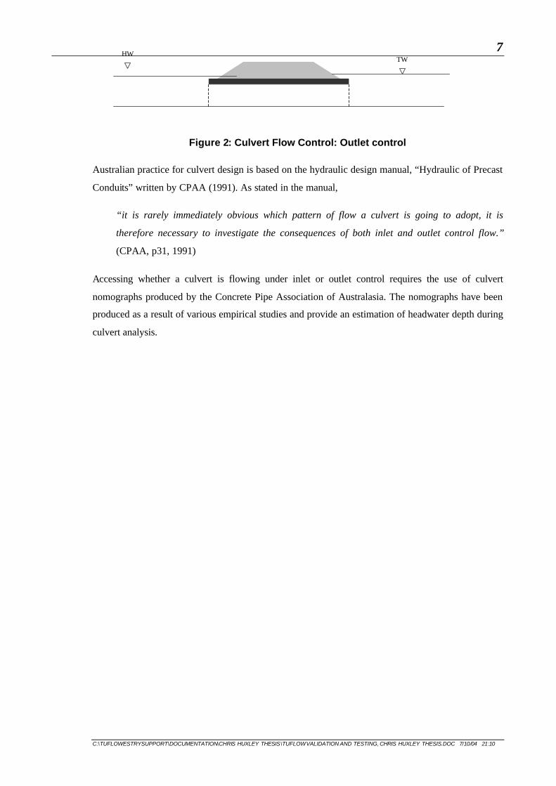
above the invert of the culvert outlet. Figure 1 and Figure 2 illustrate basic examples of inlet control
and outlet control.
Figure 1: Culvert Flow Control: Inlet control
HW
TW
7
C:\TUFLOWESTRYSUPPORT\DOCUMENTATION\CHRIS HUXLEY THESIS\TUFLOW VALIDATION AND TESTING, CHRIS HUXLEY THESIS.DOC 7/10/04 21:10
Figure 2: Culvert Flow Control: Outlet control
Australian practice for culvert design is based on the hydraulic design manual, “Hydraulic of Precast
Conduits” written by CPAA (1991). As stated in the manual,
“it is rarely immediately obvious which pattern of flow a culvert is going to adopt, it is
therefore necessary to investigate the consequences of both inlet and outlet control flow.”
(CPAA, p31, 1991)
Accessing whether a culvert is flowing under inlet or outlet control requires the use of culvert
nomographs produced by the Concrete Pipe Association of Australasia. The nomographs have been
produced as a result of various empirical studies and provide an estimation of headwater depth during
culvert analysis.
HW TW

8
C:\TUFLOWESTRYSUPPORT\DOCUMENTATION\CHRIS HUXLEY THESIS\TUFLOW VALIDATION AND TESTING, CHRIS HUXLEY THESIS.DOC 7/10/04 21:10
Figure 3: Headwater Depth for Concrete Pipe Culverts with Inlet Control
(CPAA, p34, 1991)

9
C:\TUFLOWESTRYSUPPORT\DOCUMENTATION\CHRIS HUXLEY THESIS\TUFLOW VALIDATION AND TESTING, CHRIS HUXLEY THESIS.DOC 7/10/04 21:10
Figure 4: Headwater Depth for Concrete Box Culverts with Inlet Control
(CPAA, p35, 1991)

10
C:\TUFLOWESTRYSUPPORT\DOCUMENTATION\CHRIS HUXLEY THESIS\TUFLOW VALIDATION AND TESTING, CHRIS HUXLEY THESIS.DOC 7/10/04 21:10
Figure 5: Energy Head H for Concrete Pipe Culverts Flowing Full
(CPAA, p36, 1991)

11
C:\TUFLOWESTRYSUPPORT\DOCUMENTATION\CHRIS HUXLEY THESIS\TUFLOW VALIDATION AND TESTING, CHRIS HUXLEY THESIS.DOC 7/10/04 21:10
Figure 6: Energy Head H for Concrete Box Culverts Flowing Full
(CPAA, p36, 1991)
12
C:\TUFLOWESTRYSUPPORT\DOCUMENTATION\CHRIS HUXLEY THESIS\TUFLOW VALIDATION AND TESTING, CHRIS HUXLEY THESIS.DOC 7/10/04 21:10
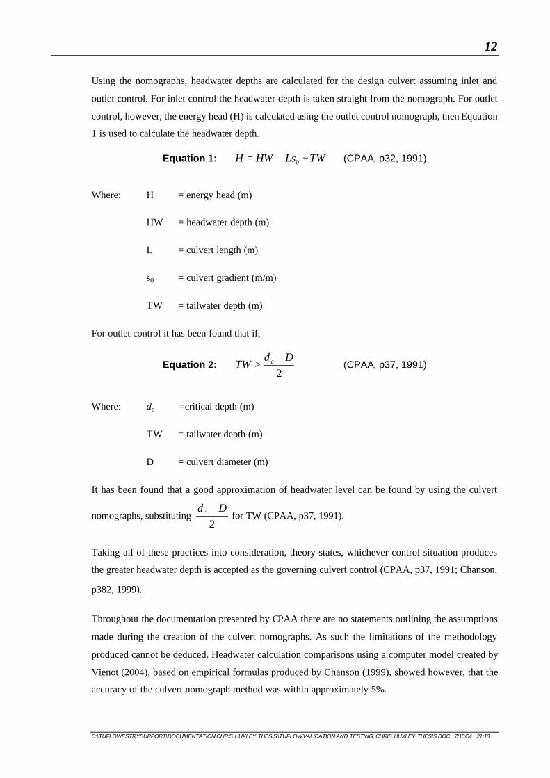
Using the nomographs, headwater depths are calculated for the design culvert assuming inlet and
outlet control. For inlet control the headwater depth is taken straight from the nomograph. For outlet
control, however, the energy head (H) is calculated using the outlet control nomograph, then Equation
1 is used to calculate the headwater depth.
Equation 1: TWLsHWH −+= 0 (CPAA, p32, 1991)
Where: H = energy head (m)
HW = headwater depth (m)
L = culvert length (m)
s0 = culvert gradient (m/m)
TW = tailwater depth (m)
For outlet control it has been found that if,
Equation 2: 2
DdTW c +
> (CPAA, p37, 1991)
Where: dc =critical depth (m)
TW = tailwater depth (m)
D = culvert diameter (m)
It has been found that a good approximation of headwater level can be found by using the culvert
nomographs, substituting 2
Ddc + for TW (CPAA, p37, 1991).
Taking all of these practices into consideration, theory states, whichever control situation produces
the greater headwater depth is accepted as the governing culvert control (CPAA, p37, 1991; Chanson,
p382, 1999).
Throughout the documentation presented by CPAA there are no statements outlining the assumptions
made during the creation of the culvert nomographs. As such the limitations of the methodology
produced cannot be deduced. Headwater calculation comparisons using a computer model created by
Vienot (2004), based on empirical formulas produced by Chanson (1999), showed however, that the
accuracy of the culvert nomograph method was within approximately 5%.

13
C:\TUFLOWESTRYSUPPORT\DOCUMENTATION\CHRIS HUXLEY THESIS\TUFLOW VALIDATION AND TESTING, CHRIS HUXLEY THESIS.DOC 7/10/04 21:10
Since it is Australian engineering practice to use the nomograph method, it will be used for the
culvert calculations during the study.
3.3.3 Weir Flow
Although there are many types of weir, in the context of this project, the only weirs being researched
are broad crested weirs. During flood events it is often the case that structures, such as road and rail
embankments or even levy banks, act as broad crested weirs. Figure 7 shows a typical schematic
representation of a broad crested weir.
Figure 7: Weir flow
Numerous laboratory-based studies have identified that there are two basic flow regimes that
determine the headwater upstream from a broad crested weir. These regimes are known as non-
submerged flow and submerged flow (Hager & Schwalt, p20, 1994). Non-submerged flow is defined
to occur when the weir inundation ratio is less than 0.75 Mathematically this is described in Equation
3. Submerged flow therefore occurs for weir flow with an inundation ratio greater than 0.75.
Non-submerged Flow
Non-submerged flow is defined to occur when the weir inundation ratio is less than 0.75
Mathematically this is described in Equation 3.
Equation 3: 75.0)()(
1
2 <−−
zdzd
Where: d2 = downstream water depth (m)
d1 = upstream water depth (m)
z = weir height (m)
For non-submerged flow it can be assumed that critical flow conditions occur on the crest of the
broad crested weir (Finnemore and Franzini, p534, 2002). Theoretically, flow at critical depth is
Energy Line
E1 d1 dc
z
w
d2
Q

14
C:\TUFLOWESTRYSUPPORT\DOCUMENTATION\CHRIS HUXLEY THESIS\TUFLOW VALIDATION AND TESTING, CHRIS HUXLEY THESIS.DOC 7/10/04 21:10
dominated by critical flow. This assumption is based on the theory that for non-submerged flow, free
overfall flow conditions occur and headwater depth is dependent solely on upstream conditions.
When calculating the upstream depth during non-submerged flow, minimum specific energy
calculations are used.
By definition the depth corresponding to the minium specific energy for a given flow is called the
specific depth, and for a rectangular channel is given by Equation 4.
Equation 4: 31
2
=
gq
d c
Where: dc = critical depth (m)
q = discharge per unit width (m3/s/m)
g = gravity (m/s2)
Using the calculated critical depth, the minimum specific energy (Emin) for the flow can be calculated
using Equation 5.
Equation 5: cdE23
min =
Where: Emin = minimum specific energy (m)
dc = critical depth (m)
Using the Minimum Specific Energy, the upstream specific energy can be calculated using Equation
6.
Equation 6: min1 EzE +=
Where E1 =upstream specific energy (m)
Emin = minimum specific energy (m)
z = height of weir (m)
Using the calculated upstream specific energy the upstream headwater depth is found using the
iterative approach given by Equation 7.

15
C:\TUFLOWESTRYSUPPORT\DOCUMENTATION\CHRIS HUXLEY THESIS\TUFLOW VALIDATION AND TESTING, CHRIS HUXLEY THESIS.DOC 7/10/04 21:10
Equation 7: 21
2
112gd
qEd −=
Where d1 = upstream depth (m)
E1 = upstream specific energy (m)
q = discharge per unit width (m3/s/m)
g = gravity (m/s2)
Submerged Flow
Submerged flow is defined to occur when the weir inundation ratio is greater than 0.75. During
submerged flow, because free overfall flow does not occur, it cannot be assumed that critical flow
conditions occur over the broad crested weir. Therefore the headwater depth is dependent on both
upstream and downstream conditions. Empirical studies conducted by Bradley (1978), published by
the US Department of Transport, have produced calibrated graphs that can be used for discharge
coefficient estimation. Figure 9 to Figure 11 show the discharge coefficient graphs and Figure 8
defines the variables used by Bradely (1978).
Figure 8: Weir Flow (Bradley, 1978)
Energy Line
H
L D

16
C:\TUFLOWESTRYSUPPORT\DOCUMENTATION\CHRIS HUXLEY THESIS\TUFLOW VALIDATION AND TESTING, CHRIS HUXLEY THESIS.DOC 7/10/04 21:10
Figure 9: Discharge Coefficient Cf (H/L>0.15)
Figure 10: Discharge coefficient Cf (H/L<0.15)
1.66
1.67
1.68
1.69
1.7
1.71
0.14 0.16 0.18 0.2 0.22 0.24 0.26 0.28 0.3
H/L
Cf
0
0.2
0.4
0.6
0.8
1
0 0.1 0.2 0.3 0.4 0.5 0.6 0.7 0.8
H(m)
Cf

17
C:\TUFLOWESTRYSUPPORT\DOCUMENTATION\CHRIS HUXLEY THESIS\TUFLOW VALIDATION AND TESTING, CHRIS HUXLEY THESIS.DOC 7/10/04 21:10
Figure 11: Discharge coefficient Cs (D/H>0.70)
As Defined by Bradley (1978), Equation 8 is used to calculate the upstream water depth H.
Equation 8: 32
=
CsCfWQ
H
Where: H = Upstream water depth (m)
Q = Upstream discharge (m3s-1)
Cs = Discharge coefficient
Cf = Discharge coeffecient
W = Weir Width (m)
Throughout the documentation presented by the Bradley (1978) there are no comments identifying
the assumptions or test methodology made during the creation of the submerged weir graphs. As such
the limitations of the methodology cannot be estimated. Other contemporary sources of literature,
however, such as “Waterway Design – A Guide to the Hydraulic design of Bridges, Culvert and
0.3
0.4
0.5
0.6
0.7
0.8
0.9
176 78 80 82 84 86 88 90 92 94 96 98 100
Inundation Ratio
Red
uctio
n Fa
ctor
Cs

18
C:\TUFLOWESTRYSUPPORT\DOCUMENTATION\CHRIS HUXLEY THESIS\TUFLOW VALIDATION AND TESTING, CHRIS HUXLEY THESIS.DOC 7/10/04 21:10
Floodways” (AUSTROADS, p17 1994), endorse the theory produced by Bradley. AUSTROADS
represents the Roads and Traffic Authorities for New South Wales, Queensland, South Australia,
Australia Capital Territory and Victoria. As both the Australian and American Road and Traffic
Authorities endorse the theory presented by Bradely (1978) it will also be used during this study.
3.3.4 Open Channel Flow
Open channel flow is characterised by a waterway, canal or conduit in which a fluid flows with a free
surface, subjected to only by atmospheric pressure (Chanson, p6, 1999; Henderson, p105, 1966).
Open channel Flow can be classified or described in various ways. One classification method is based
on the description of the flow, the flow is defined as being either uniform or non uniform.
Steady or uniform flow is defined to occur when the depth of flow within a channel is constant for a
given time interval. Unsteady or non-uniform flow, in contrast, is characteristic of flow that changes
in depth during a specified time interval.
There have been many studies based on uniform flow and as a result many uniform flow formulas are
available. The Kuttat, Bazin, Powell, Chezy and Manning formulas are examples of these. Overall,
the empirical formulas are based on the momentum equation, which states the exact balance between
the shear forces and the gravity component along a streamline (Chanson, p79, 1999).
Of the uniform flow formulas, the Manning’s formula is the most widely used because of its
simplicity and accuracy (Finnemore & Franzini, p412, 2002). The Manning’s formula is shown as
Equation 9: ASRn
Q 21
321
=
Where: n = Manning’s n roughness coeffecient
R = Hydraulic Radius (m)
S = Bed Slope (m/m)
A = Cross sectional area
Analysis of the derivation of the Manning’s formula has shown that as an empirical equation, it does
not provide exact solutions, however, it can be used as an accurate estimation of normal depth.
During the derivation of the formula, the exponent of the hydraulic radius R was based on
experimental data taken from artificial channels. For different shapes and roughness, the average
value of the exponent was found to vary from 0.6499 to 0.8395. Using these values the approximate
value of 2/3 was adopted for the exponent (Chow, p99, 1959).

19
C:\TUFLOWESTRYSUPPORT\DOCUMENTATION\CHRIS HUXLEY THESIS\TUFLOW VALIDATION AND TESTING, CHRIS HUXLEY THESIS.DOC 7/10/04 21:10
Authors such as Finnemore & Franzini (2002), Chow (1959) and Hamill (1995) recommend the use
of Manning’s formula instead other uniform flow formulas. Manning’s formula was used for the open
channel calculations throughout this study.
20
C:\TUFLOWESTRYSUPPORT\DOCUMENTATION\CHRIS HUXLEY THESIS\TUFLOW VALIDATION AND TESTING, CHRIS HUXLEY THESIS.DOC 7/10/04 21:10
4 METHODOLOGY
4.1 General
When discussing environmental models, it is recognised that the effectiveness of numerical models,
such as TUFLOW, are dependent on three main factors. These are
• the quality of physical data used during model development,
• the competence of the modeller to produce a model that is representative of the natural
system and
• the numerical capability of the model to replicate certain aspects of a given system (Barton,
p1, 2001)
To minimise the possibility of physical data affecting test results, hypothetical models were created
and used for all the testing. The use of hydraulic theory was used instead of real data to estimate
expected flow conditions for the given model case during the testing. This testing structure was
favoured for a variety of reasons. These were,
1. Elimination of possible inaccuracies in physical data.
2. The possibility for the testing of model features against an infinite number of test conditions.
During the initial scoping of the project it was realised that relying on actual physical data
may limit the possibility to test all flow regimes and variables.
The testing was structured so that the “test model” results were compared against independent
calculations based on established engineering principles. The comparison results will be calculated in
absolute terms and relative terms. The absolute variation shows the depth variation of the results in
metres, the relative variation, meanwhile, can be defined as the calculated depth variation as a percent
difference. The use of independent calculations based on engineering principles ensures the numerical
capabilities of the solution scheme utilized by the TUFLOW program is solely tested in an organised
manner.
Whilst planning the model testing, establishing the testing structure for each hydraulic feature
required the consideration of two main factors. These factors were related to the modelling structure
of TUFLOW, and the hydraulic principles describing the fluid flow.
Initially the modelling structure utilised by TUFLOW was considered. This ensured that each regime
used by the particular feature was tested. During culvert flow, for example, the modelling structure of

21
C:\TUFLOWESTRYSUPPORT\DOCUMENTATION\CHRIS HUXLEY THESIS\TUFLOW VALIDATION AND TESTING, CHRIS HUXLEY THESIS.DOC 7/10/04 21:10
TUFLOW splits the culvert flow into 12 separate flow regimes (A-J) depending on variables such as
bed slope, inlet submergence and outlet submergence.
Secondly the engineering theory used to represent the hydraulic flow was analysed. This ensured that
each flow regime and variable with relevance to the engineering theory for the hydraulic feature was
also tested. For example, open channel flow testing was conducted for supercritical, critical and
subcritical flow regimes. During each regime test, the variables of channel width, bed slope and
Manning’s roughness coefficient were also tested.
This testing structure has been used such that the testing of TUFLOW has been carried out in a
concise, structured format.
4.2 Model Structure
Developing a TUFLOW model, representative of a given system, requires a variety of different data
sets. These data sets define the transport of fluid within the model and the fluid volume entering and
leaving the model. Factors affecting fluid transport are obtained in the form of GIS layers defining
digital terrain models, hydraulic structure geometry and Manning’s roughness coefficients. Fluid
volumes entering and leaving the model extents are described as boundary conditions.
4.2.1 Fluid Transport
4.2.1.1 Digital Terrain Model
A Digital Terrain Model (DTM) is a topographic map used to define all flow paths and storage areas
within the 2D domain. It is recommended that the vertical accuracy of larger models be within 0.2m,
whilst for fine scale urban models 0.1m is recommended (WBM Oceanics Australia, p38, 2004).
4.2.1.2 Hydraulic Structures
The geometry of all hydraulic structures must be defined. This requires accurate cross section data which can often be obtained from structural plans or may need to be obtained by onsite observation and surveying.
To minimise the possibility of erroneous results during the project caused by DTM and cross section inaccuracies, hypothetical models have been used for the testing.
4.2.1.3 Manning’s Roughness Coefficient
Bed resistance values are defined for areas defined within the bounds of the DTM by an assigned Manning’s n value.

22
C:\TUFLOWESTRYSUPPORT\DOCUMENTATION\CHRIS HUXLEY THESIS\TUFLOW VALIDATION AND TESTING, CHRIS HUXLEY THESIS.DOC 7/10/04 21:10
During the testing, hypothetical models will be used, such that the full range of Manning’s n values can be tested, whilst reducing possible inaccuracies of using “real” data.
4.2.2 Boundary Conditions
Boundary conditions define the amount of fluid entering and exiting the model.
All upstream boundary conditions were assigned a QT flag, defining the boundary condition to be set
in a flow vs time format. All downstream boundary conditions were assigned a HT flag, defining the
format of the boundary condition to be, head vs time.
4.3 Model Run
Conventionally there are two types of model run which can be modelled, static and dynamic. A static
run is characterised by fixed boundary conditions, simulating uniform flow conditions. In contrast, a
dynamic run commonly has boundary conditions which change over time, characteristic of non-
uniform flow.
During the testing, static runs were used to test the accuracy of the modelling program against
independent calculations. Dynamic runs, on the other hand, were used to test the transition of flow
between regimes. For example, culvert flow dynamic runs were used to test the transition between
flow governed by inlet and outlet control.

23
C:\TUFLOWESTRYSUPPORT\DOCUMENTATION\CHRIS HUXLEY THESIS\TUFLOW VALIDATION AND TESTING, CHRIS HUXLEY THESIS.DOC 7/10/04 21:10
5 INDEPENDENT TESTING
5.1 Culvert Analysis
A culvert is a covered channel designed to pass water through an embankment, such as under a
highway, railroad or through a dam (Chanson, p365, 1999). A culvert consists of three sections, the
inlet, the throat and the outlet. In cross section a culvert may be circular (pipe culvert) or rectangular
(box culvert) in shape. In practice a culvert is designed to pass a specific flow rate with an associated
natural flood level. Its hydraulic performances are the design discharge, the upstream depth and the
maximum acceptable head loss. The hydraulic design of a culvert is basically the selection of an
optimum compromise between discharge capacity and head loss (Chanson, p369, 1999).
Culvert flow is one directional in nature. In order to obtain a better representation of the hydraulic
scenario and for computational efficiency TUFLOW utilises the 1D-modelling program, ESTRY, for
culvert analysis. ESTRY uses various culvert regimes, based on flow characteristics, to represent
culvert flow. Figure 12 and Figure 13 illustrate the culvert classifications used by ESTRY.
TW
A: Unsubmerged Entrance,Supercritical Slope
B: Submerged Entrance,Supercritical Slope
INLET CONTROL FLOW REGIMES
HW
TW
HW
TW
K: Unsubmerged Entrance,Submerged ExitCritical at Entrance
L: Submerged Entrance,Submerged ExitOrifice Flow at Entrance
HWTW
HW
Figure 12: ID inlet Control Culvert Flow Regimes
(WBM, p44-45, 2004)

24
C:\TUFLOWESTRYSUPPORT\DOCUMENTATION\CHRIS HUXLEY THESIS\TUFLOW VALIDATION AND TESTING, CHRIS HUXLEY THESIS.DOC 7/10/04 21:10
C: Unsubmerged Entrance,Critical Exit
D: Unsubmerged Entrance,Subcritical Exit
E: Submerged Entrance,Unsubmerged Exit
G: No FlowDry or Flap-Gate Closed
F: Submerged Entrance,Submerged Exit
OUTLET CONTROL FLOW REGIMES
HW
TW
HWTW
HWTWNo Flow
HW
TW
HWTW
H: Adverse Slope,Submerged Entrance
HW
TW
J: Adverse Slope,Unsubmerged Entrance(Critical or Subcritical at Exit)
HWTW
No Flow
Gate Closed
Figure 13: 1D Outlet Control Culvert Flow Regimes
(WBM, p44-45, 2004)

25
C:\TUFLOWESTRYSUPPORT\DOCUMENTATION\CHRIS HUXLEY THESIS\TUFLOW VALIDATION AND TESTING, CHRIS HUXLEY THESIS.DOC 7/10/04 21:10
5.1.1 Computational Procedure
The computational procedure used to test culvert flows consisted of three tests. Initially each culvert regime (A-K), as defined by ESTRY, was tested; secondly, culvert parameters were tested. The parameters tested were;
• Culvert length
• Culvert width
• Entry loss coefficients
• Culvert number
Finally, non-uniform flow tests were used to check the ability of ESTRY to model the transition of flow between different flow regimes, based on engineering theory. This ensures the transition between inlet and outlet controlled flow is tested.
These tests were undertaken for pipe and rectangular culverts. A summary of the simulations undertaken is provided in Table 2 and Table 3.
Table 2: Summary of Pipe Culvert Simulation – Regime test
Run Flow Regime
Inflow (ms -1)
Downstream Depth (m)
Diameter (mm)
Length (m)
Entry Loss (ke)
Upstream invert
(m)
Downstream invert
(m)
Number of
culverts
1 A 2 7.1 1500 35 0.5 7.5 7 1
2 B 6.5 8.1 1500 35 0.5 10 7 1
3 C 2 6.5 1500 35 0.5 7 7 1
4 D 0.5 8 1500 35 0.5 7 7.5 1
5 E 5 6.5 1500 35 0.5 7 7 1
6 F 8 9.2 1500 35 0.5 8 7 1
7 H 5 7.7 1500 35 0.5 6.5 7 1
8 J 2 7.7 1500 35 0.5 6.5 7 1
9 K
10 L 6.5 8.5 1500 35 0.5 10 7 1

26
C:\TUFLOWESTRYSUPPORT\DOCUMENTATION\CHRIS HUXLEY THESIS\TUFLOW VALIDATION AND TESTING, CHRIS HUXLEY THESIS.DOC 7/10/04 21:10
Table 3: Summary of Pipe Culvert Simulations - Variable Test
Run Inflow (ms -1)
Downstream Depth (m)
Diameter (mm)
Length (m)
Entry loss (ke)
Number of
culverts
Upstream invert
(m)
Downstream invert
(m)
Tailwater depth (m)
11 3.5 7.4 1500 35 0.5 1 7 6.5 0.4
12 3.5 7.4 1500 50 0.5 1 7 6.5 0.4
13 3.5 7.4 1500 20 0.5 1 7 6.5 0.4
14 3.5 7.4 1500 35 0.2 1 7 6.5 0.4
15 3.5 7.4 1500 35 0.8 1 7 6.5 0.4
16 3.5 7.4 900 35 0.5 1 7 6.5 0.4
17 3.5 7.4 2100 35 0.5 1 7 6.5 0.4
18 3.5 7.4 1500 35 0.5 2 7 6.5 0.4
19 3.5 7.4 1500 50 0.5 1 7 6.5 2.0
20 3.5 7.4 1500 20 0.5 1 7 6.5 2.0
Table 4: Summary of Rectangular Culvert Simulations - Regime Test
Run Flow Regime
Inflow (m3s-1)
Downstream Depth (m)
Height (mm)
Diameter (mm)
Length (m)
Entry Loss (ke)
Upstream invert
(m)
Downstream invert
(m)
Number of
culverts
21 A 3.5 7.1 1500 1500 35 0.5 7.5 7 1
22 B 6.5 8.1 1500 1500 35 0.5 10 7 1
23 C 2 7.1 1500 1500 35 0.5 7 7 1
24 D 0.5 8 1500 1500 35 0.5 7 7 1
25 E 5 6.5 1500 1500 35 0.5 7 7 1
26 F 8 9.2 1500 1500 35 0.5 8 7 1
27 H 5 7.7 1500 1500 35 0.5 6.5 7 1
28 J 0.5 7.1 1500 1500 35 0.5 6 7 1
29 K 5.8 8.9 1500 1500 35 0.5 10 7 1
30 L 6.5 8.5 1500 1500 35 0.5 10 7 1

27
C:\TUFLOWESTRYSUPPORT\DOCUMENTATION\CHRIS HUXLEY THESIS\TUFLOW VALIDATION AND TESTING, CHRIS HUXLEY THESIS.DOC 7/10/04 21:10
Table 5: Summary of Rectangular Culvert Simulations - Variable Test
Run Inflow (m3s-1)
Downstream Depth
(m)
Height (mm)
Width (mm)
Length (m)
Entry Loss (ke)
Number of
culverts
Upstream invert
(m)
Downstream invert
(m)
Tailwater depth (m)
31 3.5 7.4 1500 1500 35 0.5 1 7 6.5 0.4
32 3.5 7.4 1500 1500 50 0.5 1 7 6.5 0.4
33 3.5 7.4 1500 1500 20 0.5 1 7 6.5 0.4
34 3.5 7.4 1500 1500 35 0.2 1 7 6.5 0.4
35 3.5 7.4 1500 1500 35 0.8 1 7 6.5 0.4
36 3.5 7.4 1500 900 35 0.5 1 7 6.5 0.4
37 3.5 7.4 1500 2100 35 0.5 1 7 6.5 0.4
38 3.5 7.4 1500 1500 35 0.5 2 7 6.5 0.4
39 3.5 7.4 1500 1500 50 0.5 1 7 6.5 2
40 3.5 7.4 1500 1500 20 0.5 1 7 6.5 2
For non-uniform testing, a pipe culvert of 1.5m diameter and a rectangular culvert of the dimensions
1.5m x 1.5m was used. The following variables were assigned to the test culverts.
• Entry loss = 0.5
• Exit loss = 1.0
• Height contraction coefficient = 0.8
• Width contraction coefficients = 1.0
• Length = 35m
• Number of culverts =1
• Upstream and downstream invert = 7m

28
C:\TUFLOWESTRYSUPPORT\DOCUMENTATION\CHRIS HUXLEY THESIS\TUFLOW VALIDATION AND TESTING, CHRIS HUXLEY THESIS.DOC 7/10/04 21:10
Table 6: Culvert Flow - Non-uniform flow conditions
Run Time (hours) Inflow (m3s-1) Downstream Depth (m)
0 1.5 7.5
1 1.5 7.5
2 1.5 8
3 1.5 9
4 1.5 9.5
5 1.5 9
6 1.5 8
41 (pipe culvert),
42 (Rectangular culvert)
7 1.5 7.5
5.1.2 Results
5.1.2.1 Uniform Flow
A summary of the culvert test results is given graphically Figure 14 to Figure 17.
Runs 1-10 were used to test that ESTRY was representing each culvert regime (as defined by
ESTRY) accurately for pipe culverts. The test results are shown in Figure 14.
Figure 14: Pipe Culvert - Regime Results
0.00
2.00
4.00
6.00
8.00
10.00
12.00
14.00
A B C D E F H J K L
ESTRY Regime
Hea
dw
ater
Dep
th (
m)
0.00%
1.50%
3.00%
4.50%
6.00%
7.50%
9.00%
10.50%
12.00%
13.50%
15.00%
Var
iati
on
IndependentCalculations
ESTRYoutput
Variation
Nomograph accuracy

29
C:\TUFLOWESTRYSUPPORT\DOCUMENTATION\CHRIS HUXLEY THESIS\TUFLOW VALIDATION AND TESTING, CHRIS HUXLEY THESIS.DOC 7/10/04 21:10
Runs 11-20 tested the variables that contribute to headwater depth calculations for circular culverts. Listed below are the variables tested for each run.
• Run 11 - base run to which all other runs could be compared against
• Run 12 and 13 - culvert length during inlet control
• Run 14 and 15 - culvert entrance losses
• Run 16 and 17 – culvert diameter
• Run 18 – number of culverts
• Run 19 and 20 – culvert length during outlet control conditions
Figure 15: Pipe Culvert – Variable Results
0.00
2.00
4.00
6.00
8.00
10.00
12.00
14.00
Base
case
(Run
11)
length
=50m
(ic) (R
un 12
)
length
= 20
m (ic) (R
un 13
)
ke =0
.2 (R
un 14
)
ke= 0
.8 (R
un 15
)
Dia = 90
0mm (R
un 16
)
Dia =21
00mm (R
un 17
)
no cu
lverts
=2 (R
un 18
)
length
=50m
(oc)
(Run
19)
length
=20 (
oc) (R
un 20
)
Variable test
Hea
dw
ater
Dep
th (
m)
0.00%
1.50%
3.00%
4.50%
6.00%
7.50%
9.00%
10.50%
12.00%
13.50%
15.00%
Var
iati
on
Independent CalculationsESTRY outputVariation
Nomograph accuracy

30
C:\TUFLOWESTRYSUPPORT\DOCUMENTATION\CHRIS HUXLEY THESIS\TUFLOW VALIDATION AND TESTING, CHRIS HUXLEY THESIS.DOC 7/10/04 21:10
Runs 21-30 were used to test that ESTRY was representing each culvert regime accurately for box culverts. The test results are shown in Figure 16
Figure 16: Box Culvert - Regime Results
0.00
2.00
4.00
6.00
8.00
10.00
12.00
14.00
A B C D E F H J K L
ESTRY Regime
Hea
dw
ater
Dep
th (
m)
0.00%
1.50%
3.00%
4.50%
6.00%
7.50%
9.00%
10.50%
12.00%
13.50%
15.00%
Var
iati
on
IndependentCalculations
ESTRY output
Variation
Nomograph accuracy

31
C:\TUFLOWESTRYSUPPORT\DOCUMENTATION\CHRIS HUXLEY THESIS\TUFLOW VALIDATION AND TESTING, CHRIS HUXLEY THESIS.DOC 7/10/04 21:10
Runs 31-40 tested the variables that contribute to headwater depth calculations for box culverts. Listed below are the test explanations for each run.
• Run 31 - base run to which all other runs could be compared against
• Run 32 and 33 - culvert length during inlet control
• Run 34 and 35 - culvert entrance losses
• Run 36 and 37 – culvert width
• Run 38 – number of culverts
• Run 39 and 40 – culvert length during outlet control
Figure 17: Box Culvert – Variable Results
8.20
8.40
8.60
8.80
9.00
9.20
9.40
9.60
9.80
10.00
Base
case
(Run
31)
length
=50m
(ic) (R
un 32
)
length
= 20
m (ic) (R
un 33
)
ke =0
.2 (R
un 34
)
ke= 0
.8 (R
un 35
)
Width
= 90
0mm (R
un 36
)
Width
=210
0mm (R
un 37
)
no cu
lverts
=2 (R
un 38
)
length
=50m
(oc)
(Run
39)
length
=20 (
oc) (R
un 40
)
Variable test
Hea
dw
ater
Dep
th (
m)
0.00%
1.50%
3.00%
4.50%
6.00%
7.50%
9.00%
10.50%
12.00%
13.50%
15.00%
Var
iati
on
Independent CalculationsESTRY outputVariation
Nomograph accuracy

32
C:\TUFLOWESTRYSUPPORT\DOCUMENTATION\CHRIS HUXLEY THESIS\TUFLOW VALIDATION AND TESTING, CHRIS HUXLEY THESIS.DOC 7/10/04 21:10
5.1.2.2 Non-Uniform flow
Run 41 and 42 tests the transition of flow from inlet to outlet control, and vice versa. The testing has
been conducted on pipe and box culverts.
Figure 18: Pipe Culvert - Non Uniform Flow Results
Figure 19: Box Culvert - Non Uniform Flow Results
6
6.5
7
7.5
8
8.5
9
9.5
10
0:00 1:00 2:00 3:00 4:00 5:00 6:00 7:00 8:00
Time (hours)
Hea
dw
ater
Dep
th (
m)
0%
1%
2%
3%
4%
5%
6%
7%
8%
9%
10%
ESTRY OutputIndependent CalculationsDownstream depthVariation
Flow Regime
Outlet Control Inlet ControlInlet Control
6
6.5
7
7.5
8
8.5
9
9.5
10
0:00 1:00 2:00 3:00 4:00 5:00 6:00 7:00 8:00
Time (hours)
Hea
dw
ater
Dep
th (
m)
0%
1%
2%
3%
4%
5%
6%
7%
8%
9%
10%
ESTRYOutputIndependent CalculationsDownstream DepthVariation
Flow Regime
Outlet Control Inlet ControlInlet Control

33
C:\TUFLOWESTRYSUPPORT\DOCUMENTATION\CHRIS HUXLEY THESIS\TUFLOW VALIDATION AND TESTING, CHRIS HUXLEY THESIS.DOC 7/10/04 21:10
5.1.3 Discussion
The culvert testing initially tested the culvert regimes identified by the ESTRY program. Secondly,
variables affecting headwater depth based on engineering theory were tested. During the testing of the
variables it was considered important to test culvert flow under inlet and outlet control. Finally the
transition of flow between inlet and outlet control was tested.
During inlet control, theory states that conditions downstream of the culvert inlet do not contribute to
the headwater depth. This means that entry losses and culvert diameter are the dominant variables
contributing to headwater depth. Culvert length, however, has no effect on headwater depth. The
results show that ESTRY represents inlet control correctly.
Under outlet control downstream conditions influence headwater depth. In contrast to inlet controlled
flow conditions, culvert length affects headwater depth. When experiencing outlet control the results
show that ESTRY operates correctly, and as expected, the culvert length influences the headwater
depth.
The steady state model runs testing inlet and outlet controlled flow regimes indicate that ESTRY
provides accurate estimations for headwater depth. To complete the culvert analysis it was considered
necessary to also assess the capabilities of ESTRY to estimate flow that is experiencing a flow regime
change. Dynamic models were created, modelling a test culvert that was flowing initially under inlet
control. The flow was varied such that the culvert flow developed into outlet-controlled flow, after a
period of time, the culvert flow was then returned to inlet control. The testing indicated that ESTRY
effectively models the transition of flow between inlet and outlet control, for both, pipe and
rectangular culverts.
Overall, the results show that ESTRY produces results similar to predicted headwater depths using
the culvert nomograph method developed by the CPAA (1991). The variation in the results ranged
from 0.11% to 5%, equalling a maximum flow depth variation of 0.4m. The average variation of the
results was calculated to be 1.69%, which in absolute terms, is an average depth variation of 0.14m.
During the study it was expected that the ESTRY output would vary from the calculated depth by up
to 5%. This was assumed based on the creation of the culvert nomographs used for the testing. The
nomographs were produced from empirical laboratory studies and it is recognised that they are only a
method of headwater depth estimation.
Since the ESTRY results all produce values with a variation less than 5%, the testing shows that
ESTRY is representing culvert flow consistent with current engineering depth estimation practices.

34
C:\TUFLOWESTRYSUPPORT\DOCUMENTATION\CHRIS HUXLEY THESIS\TUFLOW VALIDATION AND TESTING, CHRIS HUXLEY THESIS.DOC 7/10/04 21:10
5.2 Weir Flow
A weir is an obstruction in a channel that raises the upstream water level, whilst allowing fluid flow
to pass over or through the obstruction (Streeter, p416, 1958). In practice, a weir is an accurate flow-
measuring device (Chow, p360, 1973). As such they are often designed for that purpose.
Although there are many types of weirs, in the context of this project, the only weirs being researched
are broad crested weirs. During flood events it is often the case that structures, such as road and rail
embankments or even levee banks, act as broad crested weirs. Other weir types such as the Sharp
Crested weir and the Ogee weir vary rarely occur in the natural or urbanised environments unless
they were designed for a specific purpose, such as for flow measurement. Figure 3 shows a section of
a broad crested weir.
Figure 20: Broad Crested Weir
A broad crested weir is a flat-crested structure with a flow length (L), represented by the distance
across the flow path at the weir crest, large compared with the flow thickness. The ratio of flow
length of the weir to upstream head over crest must typically be greater than 1.5 to 3 (Chow, p410,
1973).
Research has found there are typically two types of flow encountered during weir flow; these are
described as submerged and non-submerged flow.
5.2.1 Computational Procedure
TUFLOW has been designed such that a weir can be represented either as a 1D or 2D structure.
Basically, the size of the weir structure relative to the chosen grid size of the 2D domain defines
whether the weir is better suited to 1D or 2D modelling. Ideally, this means that weirs of small flow
length are often represented in 1D and weirs of greater flow length are modelled in 2D. During the
testing, both 1D and 2D structures were analysed for flow conditions which were:
Energy Line
E1 d1 dc
z
W
d2
Q

35
C:\TUFLOWESTRYSUPPORT\DOCUMENTATION\CHRIS HUXLEY THESIS\TUFLOW VALIDATION AND TESTING, CHRIS HUXLEY THESIS.DOC 7/10/04 21:10
• Non-submerged
• Submerged
• Transitional (Moving from submerged into non-submerged flow conditions).
The non-submerged and submerged flow was tested using steady state flow conditions. The
transitional testing was conducted using non-uniform flow.
5.2.1.1 1D Weir Flow
Non-submerged flow was tested varying; upstream discharge, downstream depth and the flow length
were varied. During the testing a weir with a height of 5 metres was used.
Table 7 shows the variables that were tested for free overfall flow conditions.
Table 7: 1D Non-submerged Flow
Run Upstream Discharge, Q (m3s-1)
Downstream Depth, d2 (m)
Flow Length, L (m)
1 1 4 5
2 3 4 5
3 5 4 5
4 7 4 5
5 1 4.5 5
6 3 4.5 5
7 5 4.5 5
8 7 4.5 5
9 1 5 5
10 3 5 5
11 5 5 5
12 7 5 5
13 1 4.99 5
14 3 4.99 5
15 5 4.99 5
16 7 4.99 5
17 1 4.99 10
18 3 4.99 10
19 5 4.99 10
20 7 4.99 10
21 1 4.99 20
36
C:\TUFLOWESTRYSUPPORT\DOCUMENTATION\CHRIS HUXLEY THESIS\TUFLOW VALIDATION AND TESTING, CHRIS HUXLEY THESIS.DOC 7/10/04 21:10
22 3 4.99 20
23 5 4.99 20
24 7 4.99 20
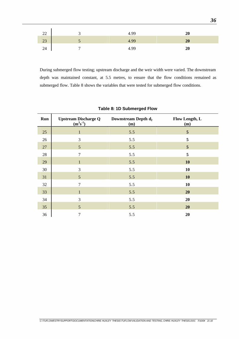
During submerged flow testing; upstream discharge and the weir width were varied. The downstream
depth was maintained constant, at 5.5 metres, to ensure that the flow conditions remained as
submerged flow. Table 8 shows the variables that were tested for submerged flow conditions.
Table 8: 1D Submerged Flow
Run Upstream Discharge Q (m3s-1)
Downstream Depth d2 (m)
Flow Length, L (m)
25 1 5.5 5
26 3 5.5 5
27 5 5.5 5
28 7 5.5 5
29 1 5.5 10
30 3 5.5 10
31 5 5.5 10
32 7 5.5 10
33 1 5.5 20
34 3 5.5 20
35 5 5.5 20
36 7 5.5 20

37
C:\TUFLOWESTRYSUPPORT\DOCUMENTATION\CHRIS HUXLEY THESIS\TUFLOW VALIDATION AND TESTING, CHRIS HUXLEY THESIS.DOC 7/10/04 21:10
The transition of flow from submerged to non-submerged flow was tested using a dynamic model,
under non-uniform flow conditions. A flow length of 5 metres and a downstream depth of 5.5 metres
were used for the testing. The upstream discharge was increased from 1m3s-1 to 16 m3s-1; this ensured
that the weir was initially flowing under submerged flow before developing into non-submerged
flow. Table 9 shows the variables that were used for transitional flow testing.
Table 9: 1D Flow Transition Test
Run Upstream Discharge, Q (m3s-1)
Time, t (hours)
Downstream Depth, d2 (m)
Flow Length, L (m)
37 1 0 5.5 5
1.5 1 5.5 5
2 2 5.5 5
2.5 3 5.5 5
3 4 5.5 5
3.5 5 5.5 5
4 6 5.5 5
4.5 7 5.5 5
5 8 5.5 5
5.5 9 5.5 5
6 10 5.5 5
6.5 11 5.5 5
7 12 5.5 5
16 13 5.5 5
5.2.1.2 2D Weir Flow
During the testing a weir with a height of 5 metres was used.
Non-submerged flow was tested varying the; upstream discharge, downstream depth and the flow
length. Table 10 shows the variables that were tested.

38
C:\TUFLOWESTRYSUPPORT\DOCUMENTATION\CHRIS HUXLEY THESIS\TUFLOW VALIDATION AND TESTING, CHRIS HUXLEY THESIS.DOC 7/10/04 21:10
Table 10: 2D Non-submerged Flow
Run Upstream Discharge Q (m3s-1)
Downstream Depth d2 (m)
Flow Length, L (m)
1 10 4 20
2 15 4 20
3 20 4 20
4 10 4.5 20
5 15 4.5 20
6 20 4.5 20
7 10 5 20
8 15 5 20
9 20 5 20
10 10 5 30
11 15 5 30
12 20 5 30
13 10 5 40
14 15 5 40
15 20 5 40
During submerged flow testing; upstream discharge and the weir width were varied. The downstream
depth was maintained constant, at 5.5 metres, to ensure that the flow conditions remained as
submerged flow. Table 11 shows the variables that were tested for submerged flow conditions.
Table 11: 2D Submerged Flow
Run Upstream Discharge, Q (m3s-1)
Downstream Depth, d2 (m)
Flow Length, L (m)
16 10 5.5 20
17 15 5.5 20
18 20 5.5 20
19 10 5.5 30
20 15 5.5 30
21 20 5.5 30
22 10 5.5 40
23 15 5.5 40
24 20 5.5 40

39
C:\TUFLOWESTRYSUPPORT\DOCUMENTATION\CHRIS HUXLEY THESIS\TUFLOW VALIDATION AND TESTING, CHRIS HUXLEY THESIS.DOC 7/10/04 21:10
The transition of flow from submerged to non-submerged flow was tested using a dynamic model.
The model used a flow length of 20 metres and a constant downstream depth of 5.5 metres. The
upstream discharge was increased from 10m3s-1 to 40 m3s-1. The change in upstream discharge, with
constant downstream depth ensured that the weir was initially flowing under submerged flow before
developing into non-submerged flow. Table 12 shows the variables that were used for transitional
flow testing.
Table 12: 2D Flow Transition Test
Run Upstream Discharge, Q (m3s-1)
Time, t (hours)
Downstream Depth, d2 (m)
Flow Length, L (m)
25 10 0 5.5 20
11 1 5.5 20
12 2 5.5 20
13 3 5.5 20
14 4 5.5 20
15 5 5.5 20
16 6 5.5 20
17 7 5.5 20
18 8 5.5 20
19 9 5.5 20
20 10 5.5 20
40 11 5.5 20

40
C:\TUFLOWESTRYSUPPORT\DOCUMENTATION\CHRIS HUXLEY THESIS\TUFLOW VALIDATION AND TESTING, CHRIS HUXLEY THESIS.DOC 7/10/04 21:10
5.2.2 Results
5.2.2.1 ID Weir Results
A summary of the 1D weir test results is given in Figure 21 to Figure 24.
Runs 1-12 were used to test that ESTRY was representing non-submerged flow accurately. During
non-submerged flow, because of free overfall conditions, the downstream depth has no influence on
the upstream depth. As expected all runs with identical upstream discharges produced identical
upstream depth estimations, independent of downstream depth. The model runs that were found to
have identical results are listed;
• Runs 1,5,9
• Runs 2,6,10
• Runs 3,7,11
• Runs 4,8,12.
The results can be seen in Table 13 this has also been graphically shown in Figure 21.
Table 13: 1D Non-submerged Flow – Results (Downstream Depth)
Run Upstream Depth Independent Calculation
(m)
Upstream Depth ESTRY Output
(m)
Variation (%)
1,5,9 5.24 5.24 0.04%
2,6,10 5.50 5.50 0.09%
3,7,11 5.70 5.71 0.13%
4,8,12 5.87 5.89 0.18%

41
C:\TUFLOWESTRYSUPPORT\DOCUMENTATION\CHRIS HUXLEY THESIS\TUFLOW VALIDATION AND TESTING, CHRIS HUXLEY THESIS.DOC 7/10/04 21:10
Figure 21: 1D Non-submerged Flow – Results (Downstream Depth)
5
5.2
5.4
5.6
5.8
6
0 1 2 3 4 5 6 7 8
Upstream Discharge Q (m3s-1)
Up
stre
am D
epth
d1
(m)
0.00%
1.00%
2.00%
3.00%
4.00%
5.00%
6.00%
7.00%
8.00%
9.00%
10.00%
Var
iati
on
Run 1-12independentcalculationsRun 1-12 ESTRYoutput
Variation

42
C:\TUFLOWESTRYSUPPORT\DOCUMENTATION\CHRIS HUXLEY THESIS\TUFLOW VALIDATION AND TESTING, CHRIS HUXLEY THESIS.DOC 7/10/04 21:10
Runs 13-24 were used to test that ESTRY was representing non-submerged flow accurately for
varying weir widths. Since upstream conditions influence downstream depth during non-submerged
flow it was expected that for wider weir widths, as defined by the continuity equation, lower
upstream depths would be produced. The results are presented in Figure 22.
Figure 22: 1D Non-submerged Flow – Results (Flow Length)
5.00
5.20
5.40
5.60
5.80
6.00
0 1 2 3 4 5 6 7 8
Upstream Discharge Q (m3s-1)
Up
stre
am D
epth
d1
(m)
0.00%
1.00%
2.00%
3.00%
4.00%
5.00%
6.00%
7.00%
8.00%
9.00%
10.00%
Var
iati
on
L=5m independentcalculations
L=5m ESTRY output
L=10m independentcalculations
L=10m ESTRY output
L=20m independentcalculations
L=20m ESTRY output
L=5m Variation
L=10m Variation
L=20m Variation
43
C:\TUFLOWESTRYSUPPORT\DOCUMENTATION\CHRIS HUXLEY THESIS\TUFLOW VALIDATION AND TESTING, CHRIS HUXLEY THESIS.DOC 7/10/04 21:10
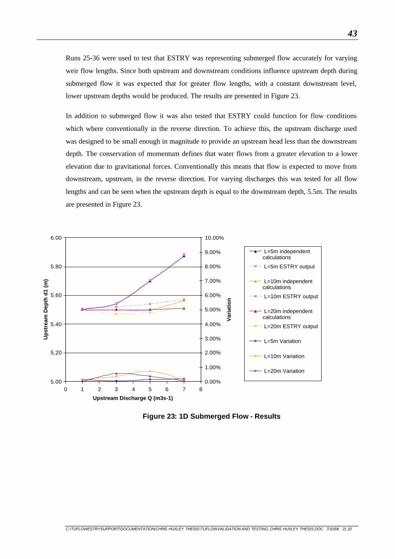
Runs 25-36 were used to test that ESTRY was representing submerged flow accurately for varying
weir flow lengths. Since both upstream and downstream conditions influence upstream depth during
submerged flow it was expected that for greater flow lengths, with a constant downstream level,
lower upstream depths would be produced. The results are presented in Figure 23.
In addition to submerged flow it was also tested that ESTRY could function for flow conditions
which where conventionally in the reverse direction. To achieve this, the upstream discharge used
was designed to be small enough in magnitude to provide an upstream head less than the downstream
depth. The conservation of momentum defines that water flows from a greater elevation to a lower
elevation due to gravitational forces. Conventionally this means that flow is expected to move from
downstream, upstream, in the reverse direction. For varying discharges this was tested for all flow
lengths and can be seen when the upstream depth is equal to the downstream depth, 5.5m. The results
are presented in Figure 23.
Figure 23: 1D Submerged Flow - Results
5.00
5.20
5.40
5.60
5.80
6.00
0 1 2 3 4 5 6 7 8
Upstream Discharge Q (m3s-1)
Up
stre
am D
epth
d1
(m)
0.00%
1.00%
2.00%
3.00%
4.00%
5.00%
6.00%
7.00%
8.00%
9.00%
10.00%
Var
iati
on
L=5m independentcalculations
L=5m ESTRY output
L=10m independentcalculations
L=10m ESTRY output
L=20m independentcalculations
L=20m ESTRY output
L=5m Variation
L=10m Variation
L=20m Variation

44
C:\TUFLOWESTRYSUPPORT\DOCUMENTATION\CHRIS HUXLEY THESIS\TUFLOW VALIDATION AND TESTING, CHRIS HUXLEY THESIS.DOC 7/10/04 21:10
Run 37 was used to test that ESTRY was representing submerged flow for varying inundation ratios accurately.
This testing method assesses whether ESTRY replicates the transition from submerged flow to unsubmerged
flow at an inundation ratio of approximately 0.75. Since both upstream and downstream conditions influence
upstream depth during submerged flow it was expected that for smaller flow rates, hence higher inundation
ratios, the upstream depth would be at its least. The results are presented in Figure 24.
Figure 24: 1D Flow Transition – Results
5.2.2.2 2D Weir Results
A summary of the 2D weir test results is given in Figure 25 to Figure 27.
Runs 1-12 were used to test that TUFLOW was representing non-submerged flow accurately. During
non-submerged flow downstream depth has no influence on the upstream depth. As expected all runs
replicating identical upstream discharges produced similar upstream depth estimations, independent
of downstream depth. The model runs that were found to have similar results are listed;
• Runs 1,4,7
• Runs 2,5,8
• Runs 3,6,9.
5.00
5.50
6.00
6.50
7.00
0 2.5 5 7.5 10 12.5 15 17.5Upstream Discharge Q (m3s-1)
Up
stre
am D
epth
d1 (
m)
0%
1%
2%
3%
4%
5%
6%
7%
8%
9%
10%
Var
iati
on
IndependentCalculations
ESTRY output
VariationTransition

45
C:\TUFLOWESTRYSUPPORT\DOCUMENTATION\CHRIS HUXLEY THESIS\TUFLOW VALIDATION AND TESTING, CHRIS HUXLEY THESIS.DOC 7/10/04 21:10
The results can be seen in
Table 14 and graphically in Figure 25.
Figure 23 uses the average upstream depth and variation of runs 1-9 for the given discharge.
Table 14: 2D Non-submerged Flow – Results (Downstream Depth)
Run Upstream Depth, d1 Independent Calculation (m)
Upstream Depth, d1 TUFLOW Output (m)
Variation (%)
1,4,7 5.24 5.470 – 5.475 0.53% - 0.62%
2,5,8 5.50 5.610 – 5.615 0.58% - 0.66%
3,6,9 5.70 5.725 – 5.732 0.45% - 0.53%
Figure 25: 2D Non-submerged Flow – Results (Downstream Depth)
5
5.2
5.4
5.6
5.8
6
9 10 11 12 13 14 15 16 17 18 19 20 21
Upstream Discharge Q (m3s-1)
Up
stre
am D
epth
d1
(m)
0%
1%
2%
3%
4%
5%
6%
7%
8%
9%
10%V
aria
tio
n
Run 1-9independentcalculations
Run 1-9 TUFLOWoutput
Variation

46
C:\TUFLOWESTRYSUPPORT\DOCUMENTATION\CHRIS HUXLEY THESIS\TUFLOW VALIDATION AND TESTING, CHRIS HUXLEY THESIS.DOC 7/10/04 21:10
Runs 7-15 were used to test that TUFLOW was representing non-submerged flow accurately for
varying weir widths. Since upstream conditions influence downstream depth during non-submerged
flow it was expected that for wider weir widths, as defined by the continuity equation, lower
upstream depths would be produced. The results are presented in Figure 26.
Figure 26: 2D Non-submerged Flow – Results (Flow Length)
Runs 16- 24 were used to test that TUFLOW was representing submerged flow for varying
inundation ratios. For each weir width, the designed discharge was varied such that for at least one
case the inundation ratio was greater than one. This implies the downstream depth is greater than the
upstream depth, hence, the weir flow is in the reverse direction. Figure 27 shows the 2D submerged
flow weir results.
5
5.2
5.4
5.6
5.8
6
9 10 11 12 13 14 15 16 17 18 19 20 21
Upstream Discharge Q (m3s-1)
Up
stre
am D
epth
d1
(m)
0%
1%
2%
3%
4%
5%
6%
7%
8%
9%
10%
Var
iati
on
L=20m independentcalculations
L=20m TUFLOWoutput
L=30m independentcalculations
L=30mTUFLOWoutput
L=40m independentcalculations
L=40m TUFLOWoutput
L =20m Variation
L=30m Variation
L=40m Variation

47
C:\TUFLOWESTRYSUPPORT\DOCUMENTATION\CHRIS HUXLEY THESIS\TUFLOW VALIDATION AND TESTING, CHRIS HUXLEY THESIS.DOC 7/10/04 21:10
Figure 27: 2D Submerged Flow - Results
Run 25 tested the transition of flow from submerged to non-submerged flow, dynamically, in 2D. For
lower discharges it was expected that lower upstream discharges would be experienced.
Figure 28: 2D Flow Transition – Results
5
5.2
5.4
5.6
5.8
6
9 10 11 12 13 14 15 16 17 18 19 20 21
Upstream Discharge Q (m3s-1)
Up
stre
am D
epth
d1
(m)
0%
1%
2%
3%
4%
5%
6%
7%
8%
9%
10%
Var
iati
on
L=20m independentcalculations
L=20m TUFLOWoutput
L=30m independentcalculations
L=30m TUFLOWoutput
L=40m independentcalculations
L=40m TUFLOWoutput
L=20m Variation
L=30m Variation
L=40m Variation
5.00
5.50
6.00
6.50
7.00
9 12.5 16 19.5 23 26.5 30 33.5 37 40.5Upstream Discharge Q (m3s-1)
Up
stre
am D
epth
d1
(m)
0%
1%
2%
3%
4%
5%
6%
7%
8%
9%
10%
Var
iatio
n
IndependentCalculations
TUFLOW output
Variation
Transition

48
C:\TUFLOWESTRYSUPPORT\DOCUMENTATION\CHRIS HUXLEY THESIS\TUFLOW VALIDATION AND TESTING, CHRIS HUXLEY THESIS.DOC 7/10/04 21:10
5.2.3 Discussion
TUFLOW is able to represent weir flow in 2D, whilst, ESTRY is used to represent weir flow in 1D.
Theoretically there are two regimes of flow that can occur at a weir, submerged and non-submerged
flow. These factors required that the weir flow be tested in 1D and 2D, for non-submerged,
submerged flow and the transition between the flow regimes.
During non-submerged flow, conditions downstream of the weir do not contribute to the upstream
water depth. Therefore, the dominant variables contributing to headwater depth are flow length and
upstream discharge. The testing was structured to test non-submerged flow for a variety of
downstream depths, upstream discharge and flow length. The results show that ESTRY and
TUFLOW represent non-submerged weir flow correctly, when compared against calculations based
on critical depth theory. The variation in the 1D results ranged from 0.04% to 0.18%, the 2D results
ranged from 0.25% - 0.66%.
Under submerged flow conditions, critical depth calculations cannot be used; instead empirical
studies by Bradley (1978) have produced engineering theory that is consistent for submerged flow.
During submerged flow conditions, upstream discharge, downstream depth and flow length are all
dominant variables contributing to upstream water depth. When comparing the ESTRY and
TUFLOW output results against the submerged flow calculations, the results show that ESTRY and
TUFLOW are working extremely efficiently. The variation in the 1D results ranged from 0.00% to
0.55%, the 2D results ranged from 0.00% - 0.34%.
The transition of flow from submerged to non-submerged flow was tested using a dynamic model
operating under non-uniform flow conditions. Steady state calculations were used to check the
validity of the ESTRY and TUFLOW output results. These were calculated at hourly intervals for
specified upstream discharges. Results show that ESTRY and TUFLOW are representing the
transition from submerged to non-submerged flow proficiently. Output results compared against the
steady state calculations show the calculated variation for 1D flow ranged from 0.02% - 0.4%, whilst
the variation for 2D flow was calculated to range from 0.00% - 0.6%.
Overall, the ESTRY and TUFLOW results produced depth estimations with a variation of less than
1% from independently calculated depths using current engineering depth estimation practices. In
absolute terms the maximum variation in depth for all the weir testing was found to be 0.04 metres.
The testing illustrates that ESTRY and TUFLOW are operating efficiently, representing weir flow
correctly.

49
C:\TUFLOWESTRYSUPPORT\DOCUMENTATION\CHRIS HUXLEY THESIS\TUFLOW VALIDATION AND TESTING, CHRIS HUXLEY THESIS.DOC 7/10/04 21:10
5.3 Open Channel Flow
Open channel flow is characterised by a waterway, canal or conduit in which a fluid flows with a free
surface, subjected to atmospheric pressure (Chanson, p6, 1999; Finnemore & Franzini, p407, 2002).
During open channel flow, flow is caused by the gravity component along the slope of the channel;
not by some external head, as is the case with pipe flow.
Figure 29: Open Channel Flow
Open channel flow typically occurs within river systems and on floodplains during flood events.
5.3.1 Computational Procedure
TUFLOW has the ability to represent open channel flow in 1D and 2D. Conventionally 1D channels
are used to represent smaller drainage elements, which cannot be accurately represented by the use of
a 2D grid mesh. The computational procedure used to test open channel flow consisted of four tests.
These were:
• 2D channel flow (ie; River flow)
• 2D floodplain flow
• 2D floodplain/ 2D channel flow
• 2D floodplain/ 1D channel flow.
For each test scenario, runs were developed testing the accuracy for a variety of:
• Channel bed slopes
Water Flow
Datum
Velocity distribution
Atmosphere
θ

50
C:\TUFLOWESTRYSUPPORT\DOCUMENTATION\CHRIS HUXLEY THESIS\TUFLOW VALIDATION AND TESTING, CHRIS HUXLEY THESIS.DOC 7/10/04 21:10
• Manning’s n
• Discharges.
Throughout testing, channel bed slope was varied from 10.4%, representing a “channel of large
slope”, to 0.02%, representing a “channel of small slope” as defined by Chow (p33, 1959).
Manning’s n values ranging from 0.02 to 0.12 were used. These values are the maximum and
minimum estimated Manning’s n values for both river and floodplain flows quoted by Chow (pp110-
113, 1959).
Finally flow discharges ranging from 800m3/s to 10m m3/s were used such that supercritical, critical
and subcritical flow conditions were tested.
5.3.1.1 2D Channel Flow
A basic rectangle channel, as shown in Figure 30, was used for the testing.
Figure 30: 2D Channel Flow Model
Table 15 shows the variables that were tested for 2D channel flow.
• Runs 1-18 use a bed slope of 10.4% testing super critical flow
• Runs 19-36 use a bed slope of 5.2% testing super critical and critical flow
• Runs 37-54 use a bed slope of 2.6% testing super critical to sub critical flow
• Runs 55-72 use a bed slope of 1.3% testing super critical to sub critical flow
• Runs 73-90 use a bed slope of 0.2% testing sub critical flow
• Runs 91-108 use a bed slope of 0.02% testing sub critical flow
20m
5m

51
C:\TUFLOWESTRYSUPPORT\DOCUMENTATION\CHRIS HUXLEY THESIS\TUFLOW VALIDATION AND TESTING, CHRIS HUXLEY THESIS.DOC 7/10/04 21:10
Table 15: 2D Channel Flow Variables
Discharge (m3s-1)
Mannings n 10 20 30
0.02 Run
1,19,37,55,73,91
Run
7,25,43,61,80,97
Run
13,31,49,67,86,103
0.04 Run
2,20,38,56,74,92
Run
8,26,44,62,81,98
Run
14,32,50,68,87,104
0.06 Run
3,21,39,57,75,93
Run
9,27,45,63,82,99
Run
15,33,51,69,88,105
0.08 Run
4,22,40,58,76,94
Run
10,28,46,64,83,100
Run
16,34,52,70,89,106
0.10 Run
5,23,41,59,78,95
Run
11,29,47,65,84,101
Run
17,35,53,71,90,107
0.12 Run
6,24,42,60,79,96
Run
12,30,48,66,85,102
Run
18,36,54,72,91,108
5.3.1.2 2D Floodplain Flow
A simple rectangular floodplain, as shown in Figure 30, was used for the testing. The width of the
floodplain was made sufficiently large enough to ensure that the width is greater than 10 times the
flow depth. As defined by Chow (p27, 1957) this classifies the floodplain as a “wide open channel”.
Figure 31: 2D Floodplain Flow Model
145m
15

52
C:\TUFLOWESTRYSUPPORT\DOCUMENTATION\CHRIS HUXLEY THESIS\TUFLOW VALIDATION AND TESTING, CHRIS HUXLEY THESIS.DOC 7/10/04 21:10
Table 15 shows the variables that were tested for 2D floodplain flow.
• Runs 1-18 use a bed slope of 10.4% testing super critical flow
• Runs 19-36 use a bed slope of 5.2% testing super critical and critical flow
• Runs 37-54 use a bed slope of 2.6% testing super critical to sub critical flow
• Runs 55-72 use a bed slope of 1.3% testing super critical to sub critical flow
• Runs 73-90 use a bed slope of 0.2% testing sub critical flow
• Runs 91-108 use a bed slope of 0.02% testing sub critical flow
Table 16: 2D Channel Flow Variables
Discharge (m3s-1)
Mannings n 100 200 300
0.02 Run
1,19,37,55,73,91
Run
7,25,43,61,80,97
Run
13,31,49,67,86,103
0.04 Run
2,20,38,56,74,92
Run
8,26,44,62,81,98
Run
14,32,50,68,87,104
0.06 Run
3,21,39,57,75,93
Run
9,27,45,63,82,99
Run
15,33,51,69,88,105
0.08 Run
4,22,40,58,76,94
Run
10,28,46,64,83,100
Run
16,34,52,70,89,106
0.10 Run
5,23,41,59,78,95
Run
11,29,47,65,84,101
Run
17,35,53,71,90,107
0.12 Run
6,24,42,60,79,96
Run
12,30,48,66,85,102
Run
18,36,54,72,91,108

53
C:\TUFLOWESTRYSUPPORT\DOCUMENTATION\CHRIS HUXLEY THESIS\TUFLOW VALIDATION AND TESTING, CHRIS HUXLEY THESIS.DOC 7/10/04 21:10
5.3.1.3 2D Floodplain Flow/ Channel Flow
Tests models were developed to represent compound channel flow, when the flow is not solely
confined to the channel. A simple floodplain/channel scenario, as shown in Figure 32 was used for
the testing. The testing was modelled using steady and non-steady state flow conditions.
Figure 32: 2D Floodplain/ Channel Flow Model
The models were created to replicate both steep and flat-sloped floodplain/channel cases.
• Steady state runs 1-18 and non steady state runs 37-42 use a bed slope of 1.3%
• Steady state runs 19-36 and non steady state runs 43-48 use a bed slope of 0.02%
Throughout the testing the Manning’s n roughness coefficient for the channel was fixed at 0.05. The
Manning’s n coefficient of the floodplain and the upstream discharge were varied during the testing,
as is shown in Table 17 and Table 18. For the non-steady state testing the upstream discharge was
varied from 300m3/s to 800 m3/s over a period of 3 hours. The flows agreement was defined as:
• Time = 0 (hours), Discharge = 300 (m3/s)
• Time = 1 (hours), Discharge = 500 (m3/s)
• Time = 2 (hours), Discharge = 800 (m3/s).
The model tests were conducted for 2D floodplain/2D channel and 2D floodplain/1D channel
configurations.
40m 20m 75m
5m Depth y (m)

54
C:\TUFLOWESTRYSUPPORT\DOCUMENTATION\CHRIS HUXLEY THESIS\TUFLOW VALIDATION AND TESTING, CHRIS HUXLEY THESIS.DOC 7/10/04 21:10
Table 17: 2D Floodplain/ Channel Flow Variables (Steady State)
Discharge (m3s-1)
Manning’s n 300 500 800
0.02 Run 1, 19 Run 7, 25 Run 13, 31
0.04 Run 2, 20 Run 8, 26 Run 14, 32
0.06 Run 3, 21 Run 9, 27 Run 15, 33
0.08 Run 4, 22 Run 10, 28 Run 16, 34
0.10 Run 5, 23 Run 11, 29 Run 17, 35
0.12 Run 6, 24 Run 12, 30 Run 18, 36
Table 18: 2D Floodplain/ Channel Flow Variables (Non-Steady State)
Manning’s n Run
0.02 Run 37, 43
0.04 Run 38, 44
0.06 Run 39, 45
0.08 Run 40, 46
0.10 Run 41, 47
0.12 Run 42, 48

55
C:\TUFLOWESTRYSUPPORT\DOCUMENTATION\CHRIS HUXLEY THESIS\TUFLOW VALIDATION AND TESTING, CHRIS HUXLEY THESIS.DOC 7/10/04 21:10
5.3.2 Results
5.3.2.1 2D Channel Flow and 2D Floodplain Flow
2D channel and 2D floodplain flow was tested for a variety of bed slopes, upstream discharge and
Manning’s n roughness coefficients. The testing structure was
• Runs 1-18 test for a steep bed slope (>10%), typical of the upper reaches of a coastal river or
stream. The tests check whether TUFLOW can represent supercritical flow conditions in 2D
channel flow situations. The test results are presented in Figure 33 for 2D channel flow
Figure 39 and for 2D floodplain flow.
• Runs 19-36 test for a mild bed slope, typical of the upper reaches of a coastal river or stream.
The testing checks that TUFLOW can represent supercritical and critical flow conditions
when replicating 2D channel flow cases. The test results are presented in Figure 34 for 2D
channel flow Figure 40 and for 2D floodplain flow.
• Runs 37-54 where designed to test the 2D channel flow for a small slope (<10%), typical of
the middle reaches of a coastal river or stream. The testing checks that TUFLOW can
represent supercritical, critical and subcritical flow conditions for 2D channel flow cases. The
test results are presented in Figure 35 for 2D channel flow and Figure 41 for 2D floodplain
flow.
• Runs 55-72 where designed to test the 2D channel flow for a small slope, typical of the
middle reaches of a coastal river or stream. The testing checks that TUFLOW can represent
supercritical, critical and subcritical flow conditions for 2D channel flow cases. The test
results are presented in Figure 36 for 2D channel flow and Figure 42 for 2D floodplain flow.
• Runs 73-108 test for a very small bed slope, typical of the middle/lower reaches of a coastal
river or stream. The testing checks that TUFLOW can represent subcritical flow conditions
for 2D channel flow cases. The test results are presented in Figure 37 and Figure 38 for 2D
channel flow and Figure 43 and Figure 44 for 2D floodplain flow.
It was expected that for greater flow rates and increased Manning’s n roughness coefficients, the
corresponding flow depth would increase. The test results are presented in Figure 33.

56
C:\TUFLOWESTRYSUPPORT\DOCUMENTATION\CHRIS HUXLEY THESIS\TUFLOW VALIDATION AND TESTING, CHRIS HUXLEY THESIS.DOC 7/10/04 21:10
Figure 33: 2D Channel Flow Results- Slope= 10.4%
Figure 34: 2D Channel Flow Results- Slope= 5.2%
Supercritical flow = Runs 1-10, 13-14, 20-23, 25-26, 31
Critical flow = Runs 15, 24, 27, 32
Subcritical flow = Runs 11-12, 16-19, 28-30, 33-36
0.0
0.5
1.0
1.5
2.0
2.5
3.0
3.5
4.0
4.5
5.0
18 19 20 21 22 23 24 25 26 27 28 29 30 31 32 33 34 35 36 37
Run
Dep
th (m
)
0%
1%
2%
3%
4%
5%
6%
7%
8%
9%
10%
Var
iati
on
Independent CalculationsTUFLOW Output Variation
10 20 30Discharge (m3/s)
0.000
0.500
1.000
1.500
2.000
2.500
3.000
3.500
4.000
4.500
5.000
0 1 2 3 4 5 6 7 8 9 10 11 12 13 14 15 16 17 18 19
Run
Dep
th (
m)
0%
1%
2%
3%
4%
5%
6%
7%
8%
9%
10%
Discharge (m3/s)
Var
iati
on
Independent CalculationsTUFLOW Output Variation
10 20 30

57
C:\TUFLOWESTRYSUPPORT\DOCUMENTATION\CHRIS HUXLEY THESIS\TUFLOW VALIDATION AND TESTING, CHRIS HUXLEY THESIS.DOC 7/10/04 21:10
Figure 35: 2D Channel Flow Results- Slope= 2.6%
Figure 36: 2D Channel Flow Results- Slope= 1.3%
Supercritical flow = Runs 36-39, 43-44, 49, 54-56, 61, 67
Critical flow = Runs 40, 57, 67
Subcritical flow = Runs 41-42, 45-48, 50-55, 58-60, 62-66, 68-72
0.0
0.5
1.0
1.5
2.0
2.5
3.0
3.5
4.0
4.5
5.0
36 37 38 39 40 41 42 43 44 45 46 47 48 49 50 51 52 53 54 55
Run
Dep
th (
m)
0%
1%
2%
3%
4%
5%
6%
7%
8%
9%
10%
Var
iati
on
Independent CalculationsTUFLOW Output Variation
10 20 30
Discharge (m3/s)
0.0
0.5
1.0
1.5
2.0
2.5
3.0
3.5
4.0
4.5
5.0
54 55 56 57 58 59 60 61 62 63 64 65 66 67 68 69 70 71 72 73
Run
Dep
th (
m)
0%
1%
2%
3%
4%
5%
6%
7%
8%
9%
10%
Var
iati
on
Independent CalculationsTUFLOW Output Variation
10 20 30
Discharge (m3/s)

58
C:\TUFLOWESTRYSUPPORT\DOCUMENTATION\CHRIS HUXLEY THESIS\TUFLOW VALIDATION AND TESTING, CHRIS HUXLEY THESIS.DOC 7/10/04 21:10
Figure 37: 2D Channel Flow Results- Slope= 0.2%
Figure 38: 2D Channel Flow Results- Slope= 0.02%
Supercritical flow = Run 73
Subcritical flow = Runs 74-108
0.000
0.500
1.000
1.500
2.000
2.500
3.000
3.500
4.000
4.500
5.000
72 73 74 75 76 77 78 79 80 81 82 83 84 85 86 87 88 89 90 91
Run
Dep
th (
m)
0%
1%
2%
3%
4%
5%
6%
7%
8%
9%
10%
Var
iati
on
Independent CalculationsTUFLOW Output Variation
10 20 30
Discharge (m3/s)
0.000
0.500
1.000
1.500
2.000
2.500
3.000
3.500
4.000
4.500
5.000
90 91 92 93 94 95 96 97 98 99 100
101
102
103
104
105
106
107
108
109
Run
Dep
th (m
)
0.000%
1.000%
2.000%
3.000%
4.000%
5.000%
6.000%
7.000%
8.000%
9.000%
10.000%
Var
iatio
n
Independent CalculationsTUFLOW Output Variation
10 20 30
Discharge (m3/s)

59
C:\TUFLOWESTRYSUPPORT\DOCUMENTATION\CHRIS HUXLEY THESIS\TUFLOW VALIDATION AND TESTING, CHRIS HUXLEY THESIS.DOC 7/10/04 21:10
Figure 39: 2D Floodplain Flow Results- Slope= 10.4%
Figure 40: 2D Floodplain Flow Results- Slope= 5.2%
Supercritical flow = Runs 1-3, 7-10, 13-16, 19-20, 25-26, 31-33
Critical flow = Runs 4, 11, 17, 21, 27
Subcritical flow = Runs 5-6, 12, 18-19, 22-24, 28-30, 34-36
0
1
2
3
4
5
6
0 1 2 3 4 5 6 7 8 9 10 11 12 13 14 15 16 17 18 19
Run
Dep
th (
m)
0%
1%
2%
3%
4%
5%
6%
7%
8%
9%
10%
Var
iati
on
IndependentCalculationsTUFLOWOutputVariation
100 200 300
Discharge (m3/s)
0
1
2
3
4
5
6
18 19 20 21 22 23 24 25 26 27 28 29 30 31 32 33 34 35 36 37
Run
Dep
th (
m)
0%
1%
2%
3%
4%
5%
6%
7%
8%
9%
10%V
aria
tio
n
IndependentCalculationsTUFLOWOutputVariation
100 200 300
Discharge (m3/s)

60
C:\TUFLOWESTRYSUPPORT\DOCUMENTATION\CHRIS HUXLEY THESIS\TUFLOW VALIDATION AND TESTING, CHRIS HUXLEY THESIS.DOC 7/10/04 21:10
Figure 41: 2D Floodplain Flow Results – Slope = 2.6%
Figure 42: 2D Floodplain Flow Results – Slope = 1.3%
Supercritical flow = Runs 37, 43-44, 49-50, 55, 61, 67
Critical flow = Run 38
Subcritical flow = Runs 39-42, 45-48, 51-54, 56-60, 62-66, 68-72
0
1
2
3
4
5
6
36 37 38 39 40 41 42 43 44 45 46 47 48 49 50 51 52 53 54 55
Run
Dep
th (
m)
0%
1%
2%
3%
4%
5%
6%
7%
8%
9%
10%
Var
iati
on
IndependentCalculationsTUFLOW Output
Variation
100 200 300
Discharge (m3/s)
0
1
2
3
4
5
6
54 55 56 57 58 59 60 61 62 63 64 65 66 67 68 69 70 71 72 73
Run
Dep
th (
m)
0%
1%
2%
3%
4%
5%
6%
7%
8%
9%
10%V
aria
tio
n
IndependentCalculationsTUFLOW Output
Variation
100 200 300
Discharge (m3/s)

61
C:\TUFLOWESTRYSUPPORT\DOCUMENTATION\CHRIS HUXLEY THESIS\TUFLOW VALIDATION AND TESTING, CHRIS HUXLEY THESIS.DOC 7/10/04 21:10
Figure 43: 2D Floodplain Flow Results – Slope = 0.2%
Figure 44: 2D Floodplain Flow Results – Slope = 0.02%
Subcritical flow = Runs 73-108
0
1
2
3
4
5
6
72 73 74 75 76 77 78 79 80 81 82 83 84 85 86 87 88 89 90 91
Run
Dep
th (
m)
0%
1%
2%
3%
4%
5%
6%
7%
8%
9%
10%
Var
iati
on
IndependentCalculationsTUFLOWOutputVariation
100 200 300
Discharge (m3/s)
0
1
2
3
4
5
6
90 91 92 93 94 95 96 97 98 99 100
101
102
103
104
105
106
107
108
109
Run
Dep
th (
m)
0%
1%
2%
3%
4%
5%
6%
7%
8%
9%
10%V
aria
tio
n
IndependentCalculationsTUFLOWOutputVariation
100 200 300
Discharge (m3/s)

62
C:\TUFLOWESTRYSUPPORT\DOCUMENTATION\CHRIS HUXLEY THESIS\TUFLOW VALIDATION AND TESTING, CHRIS HUXLEY THESIS.DOC 7/10/04 21:10
5.3.2.2 2D Floodplain Flow/ 2D Channel Flow
Runs 1-18 were used to test the transition from 2D channel flow, to 2D floodplain/ 2D channel flow.
Runs 1-12 were designed to use a flow rate insufficient to require floodplain flow. Runs 13-18,
however, were assigned a flow rate large enough to require floodplain flow. All runs were designed
to reach steady state. The results are presented in Figure 45. Figure 46 shows the results of the non-
steady state testing.
Figure 45: 2D Floodplain/2D Channel Flow Results – Slope = 1.3% (Steady State)
0
2
4
6
8
10
12
14
16
0 1 2 3 4 5 6 7 8 9 10 11 12 13 14 15 16 17 18 19
Run
Dep
th (
m)
0%
1%
2%
3%
4%
5%
6%
7%
8%
9%
10%
Var
iati
on
Calculated depth (m)TUFLOW OutputVariation
Discharge m3s-1
300 500 800

63
C:\TUFLOWESTRYSUPPORT\DOCUMENTATION\CHRIS HUXLEY THESIS\TUFLOW VALIDATION AND TESTING, CHRIS HUXLEY THESIS.DOC 7/10/04 21:10
Figure 46: 2D Floodplain/2D Channel Flow Results – Slope = 1.3% (Non-Uniform Flow)
Runs 19-36 were used to test compound channel flow for a very small bed slope, typical of a coastal
floodplain/river. The results are presented in Figure 47. Figure 48 illustrates the results of the non-
uniform flow testing.
Figure 47: 2D Floodplain/2D Channel Flow Results – Slope = 0.02% (Steady State)
0
2
4
6
8
10
12
14
16
18 19 20 21 22 23 24 25 26 27 28 29 30 31 32 33 34 35 36 37
Runs
Dep
th (m
)
0%
1%
2%
3%
4%
5%
6%
7%
8%
9%
10%
Calculated depth (m)TUFLOW OutputVariation
Discharge m3s-1
300 500 800
0
1
2
3
4
5
6
7
250 350 450 550 650 750 850
Discharge (m3s-1)
Dep
th (m
)
TUFLOW Outputn=0.12
TUFLOW Outputn=0.10
TUFLOW Outputn=0.08
TUFLOW Outputn=0.06
TUFLOW Outputn=0.04
TUFLOW Outputn=0.02
Calculated depth

64
C:\TUFLOWESTRYSUPPORT\DOCUMENTATION\CHRIS HUXLEY THESIS\TUFLOW VALIDATION AND TESTING, CHRIS HUXLEY THESIS.DOC 7/10/04 21:10
Figure 48: 2D Floodplain/2D Channel Flow Results – Slope = 0.02% (Non-Uniform Flow)
0
2
4
6
8
10
12
14
16
250 350 450 550 650 750 850
Discharge (m3s-1)
Dep
th (m
)
TUFLOW Outputn=0.12
TUFLOW Outputn=0.10
TUFLOW Outputn=0.08
TUFLOW Outputn=0.06
TUFLOW Outputn=0.04
TUFLOW Outputn=0.02
Calculated Depth

65
C:\TUFLOWESTRYSUPPORT\DOCUMENTATION\CHRIS HUXLEY THESIS\TUFLOW VALIDATION AND TESTING, CHRIS HUXLEY THESIS.DOC 7/10/04 21:10
5.3.2.3 2D Floodplain Flow/ 1D Channel Flow
Runs 1-18 were used to test the 2D floodplain/ 1D channel flow. Runs 1-12 were designed to use a
flow rate insufficient to require floodplain flow, as such the flow is confined to the channel. Runs 13-
18, were assigned a flow rate great enough to require floodplain flow. All runs were designed for
uniform flow conditions. The results are presented in Figure 45. Figure 46 shows the results of the
non-uniform testing. During the non-uniform flow testing the upstream discharge ranged from
300m3s-1 to 800m3s-1 over a 3 hour period.
Figure 49: 2D Floodplain/1D Channel Flow Results – Slope = 1.3% (Steady State)
0
2
4
6
8
10
12
14
16
0 1 2 3 4 5 6 7 8 9 10 11 12 13 14 15 16 17 18 19
Run
Dep
th (m
)
0%
1%
2%
3%
4%
5%
6%
7%
8%
9%
10%
Var
iatio
nCalculated depth (m)TUFLOW Output
Discharge m3s-1
300 500 800

66
C:\TUFLOWESTRYSUPPORT\DOCUMENTATION\CHRIS HUXLEY THESIS\TUFLOW VALIDATION AND TESTING, CHRIS HUXLEY THESIS.DOC 7/10/04 21:10
Figure 50: 2D Floodplain/2D Channel Flow Results – Slope = 1.3% (Non-Uniform Flow)
Runs 19-36 were used to test compound channel flow for a very small bed slope, typical of a coastal
floodplain/river. The results are presented in Figure 47. Figure 48 illustrates the results of the non-
uniform flow testing.
0
1
2
3
4
5
6
7
0 1 2
Time (hours)
Dep
th (m
)
TUFLOW Outputn=0.12
TUFLOW Outputn=0.10
TUFLOW Outputn=0.08
TUFLOW Outputn=0.06
TUFLOW Outputn=0.04
TUFLOW Outputn=0.02
Calculated depth

67
C:\TUFLOWESTRYSUPPORT\DOCUMENTATION\CHRIS HUXLEY THESIS\TUFLOW VALIDATION AND TESTING, CHRIS HUXLEY THESIS.DOC 7/10/04 21:10
Figure 51: 2D Floodplain/1D Channel Flow Results – Slope = 0.02% (Steady State)
Figure 52: 2D Floodplain/1D Channel Flow Results – Slope = 0.02% (Non-Uniform Flow)
0
2
4
6
8
10
12
14
16
18 19 20 21 22 23 24 25 26 27 28 29 30 31 32 33 34 35 36 37
Runs
Dep
th (
m)
0%
1%
2%
3%
4%
5%
6%
7%
8%
9%
10%
Calculated depth (m)TUFLOW OutputVariation
Discharge m3s-1
300 500 800
0
2
4
6
8
10
12
14
16
0 1 2
Time (hours)
Dep
th (m
)
TUFLOW Outputn=0.12
TUFLOW Outputn=0.10
TUFLOW Outputn=0.08
TUFLOW Outputn=0.06
TUFLOW Outputn=0.04
TUFLOW Outputn=0.02
Calculated Depth

68
C:\TUFLOWESTRYSUPPORT\DOCUMENTATION\CHRIS HUXLEY THESIS\TUFLOW VALIDATION AND TESTING, CHRIS HUXLEY THESIS.DOC 7/10/04 21:10
5.3.3 Discussion
As defined by the Froude number, open channel flow can be described by three flow regimes,
subcritical, critical and supercritical flow. These flow regimes were tested during the floodplain and
channel testing. Based on the modelling structure utilised by TUFLOW, compound channel flow was
tested using steady state and dynamic boundary conditions. The deeper main channel was represented
in both 1D and 2D.
Studies have shown that various implicit solution schemes for the 2D SWE experience problems
when used for hydraulic calculations during supercritical flow (Kutijar & Hewett, p2, 2002). For this
reason, it was considered important to test open channel flow for supercritical flow. To achieve this,
floodplains and channels with steep bed slopes were used. It should be noted, however, the geometry
of the test models used during the testing did not model the representation of hydraulic situations such
as hydraulic jumps or the surcharging of water against obstructions. As these situations are
characterised by 3D localised effects, further study is required to assess TUFLOW’s capabilities to
model these situations.
The results of the 2D floodplain and 2D channel testing show that the solution scheme utilised by the
TUFLOW program operates accurately for all flow conditions.
The calculated depths using the Manning equation the 2D channel results showed a variation in depth
ranging from 0.48% to 0.00%. The 2D floodplain testing showed a variation in water depth ranging
from 1.35% to 0.27%.
Compound channel configurations were tested using uniform and non-uniform boundary conditions.
In both cases steady state calculations were used to check the validity of the TUFLOW output results.
For the non-uniform flow conditions these were calculated at hourly intervals for specified upstream
discharges. Results show TUFLOW represents compound channel flow correctly. Overall the results
from the fully 2D model and the 1D/2D model were comparable. The fully 2D model produced water
depth results with a variation ranging from 1.201% to 0.097%. The 1D/2D models in comparison
produced a variation between 0.779% and 0.92%.
The TUFLOW results produce depth estimations with a variation of less than 1.5% from
independently calculated depths using theory based on the Manning equation. Overall, the greatest
variation in depth was found to be 0.06m for the open channel flow test cases. The testing shows that
TUFLOW represents open flow correctly for the test cases examined.

69
C:\TUFLOWESTRYSUPPORT\DOCUMENTATION\CHRIS HUXLEY THESIS\TUFLOW VALIDATION AND TESTING, CHRIS HUXLEY THESIS.DOC 7/10/04 21:10
5.4 TUFLOW Performance
5.4.1 Computational Procedure
The combined data for culvert, weir and open channel flow was pooled to assess the overall
performance of the TUFLOW program for the cases considered as part of this study.
5.4.2 Results
The combined data results, cumulatively presenting the total variation in flow depth, is shown in Figure 53, a summary of these results is also presented in Table 19
Figure 53: TUFLOW Performance – Variation in Flow Depth
Table 19: TUFLOW Performance – Variation in Flow Depth (Summary)
Variation in Flow Depth (m) Percent occurrence (%)
Less than ±0.05m 88.3%
Less than ±0.10m 94.7%
Less than ±0.15m 96.3%
Less than ±0.20m 97.9%
0%
5%
10%
15%
20%
25%
30%
35%
40%
-0.8 -0.6 -0.4 -0.2 0 0.2 0.4 0.6 0.8
Model variation from calculated flow depths (m)
Per
cent
occ
uren
ce (
%)

70
C:\TUFLOWESTRYSUPPORT\DOCUMENTATION\CHRIS HUXLEY THESIS\TUFLOW VALIDATION AND TESTING, CHRIS HUXLEY THESIS.DOC 7/10/04 21:10
The combined data results for variation in flow depth, as a function of percent variation, is
graphically shown in figure 54, a summary of the results is also presented in Table 20. The percent
variation is calculated using the variation in flow depth relative to the expected calculated depth.
Figure 54: TUFLOW Performance – Percent Variation
Table 20: TUFLOW Performance – Percent Variation (Summary)
Variation in Flow Depth (%) Percent occurrence (%)
Less than ±0.5% 66.4%
Less than ±1.0% 91.1%
Less than ±1.5% 96.7%
Less than ±2.0% 97.2%
0%
5%
10%
15%
20%
25%
30%
35%
40%
-10% -8% -6% -4% -2% 0% 2% 4% 6% 8% 10%
Model variation from calculated flow depths (%)
Per
cent
occ
uren
ce (
%)

71
C:\TUFLOWESTRYSUPPORT\DOCUMENTATION\CHRIS HUXLEY THESIS\TUFLOW VALIDATION AND TESTING, CHRIS HUXLEY THESIS.DOC 7/10/04 21:10
5.4.3 Discussion
The absolute variation of the TUFLOW results is represented by the variation in depth, measured in
metres. Meanwhile, the relative variation of the TUFLOW results is presented as variation in depth,
measured by percent. The culmination of the test results show TUFLOW is producing accurate
results for the cases considered as part on this study.
The results show that approximately 98% of the time TUFLOW produced results within ±0.2m of the
predicted water depth values, estimated using current engineering theories and principles. Relative to
the estimated water depth, TUFLOW produced results within ±2% of the estimated depth
approximately 97% of the time.

72
C:\TUFLOWESTRYSUPPORT\DOCUMENTATION\CHRIS HUXLEY THESIS\TUFLOW VALIDATION AND TESTING, CHRIS HUXLEY THESIS.DOC 7/10/04 21:10
6 CONCLUSIONS
A summary of the conclusions made, based on the results of this study are provided below;
On the basis of this study TUFLOW has been found to model culvert flow, weir flow and open
channel flow accurately.
• The Culvert flow results showed the computed headwater depths calculated by ESTRY to
have a maximum variation of 5%, which is equivalent to 0.4m, when compared against
calculated headwater depths based on culvert nomographs produced by the CPAA (1991).
The average variation was found to be 1.69% or, in terms of flow depth 0.14m. Due to
inaccuracies in the culvert nomograph method these are considered acceptable results. The
testing proved that ESTRY can estimate culvert headwater depths for inlet and outlet
controlled situations.
• The weir flow results showed that ESTRY and TUFLOW accurately predict upstream water
depths for submerged and non-submerged weir flow. The maximum variation of 0.66%, in
absolute terms, 0.04m, was calculated during a comparison between the upstream depth
computed by TUFLOW, and calculation based on the specific energy equation. The average
variation in results was found to be 0.2%, which is equal to 0.014m. The testing validates
TUFLOW and ESTRY’s capabilities to estimate upstream depth for weir flow, during
submerged and non-submerged flow.
• Water depths are accurately estimated by TUFLOW for open channel flow. The results show
the computed water depths calculated by TUFLOW to have a maximum variation of 1.35%,
or 0.06m, compared with water depth estimations based on the Manning’s equation. The
average depth variation was calculated to be 0.15%, which is also equal to 0.015m
Overall the results show that
• The Stelling solution scheme utilised by the TUFLOW program solves the 2D SWE, which
mathematically represents the unsteady free surface flow of long waves, accurately. This
implies, and the testing proves, that TUFLOW estimates hydraulic process accurately.
• The hydraulic structure equations used by ESTRY replicate hydraulic processes accurately.
This study has found no areas where the TUFLOW program could possibly be further developed or
improved, increasing the accuracy of the programs hydrodynamic/ hydraulic flow estimation
capabilities.

73
C:\TUFLOWESTRYSUPPORT\DOCUMENTATION\CHRIS HUXLEY THESIS\TUFLOW VALIDATION AND TESTING, CHRIS HUXLEY THESIS.DOC 7/10/04 21:10
7 RECOMMENDATIONS
To complete the testing/validation of the TUFLOW program it is recommended that further testing is
required. Listed below are the various tests that are recommended for further testing/ validation of the
TUFLOW program.
• The testing of the interaction of fluid flow between hydraulic features. Such as, open
channel flow combined with culvert flow.
• Global sensitivity analysis of all features modelled by the TUFLOW program.

A-1
C:\TUFLOWESTRYSUPPORT\DOCUMENTATION\CHRIS HUXLEY THESIS\TUFLOW VALIDATION AND TESTING, CHRIS HUXLEY THESIS.DOC 7/10/04 21:10
APPENDIX A: CULVERT FLOW
Results Table 21: Pipe Culvert - Regime Results
Run ESTRY Regime
ESTRY Headwater Depth Output (m)
Nomograph Headwater Depth Calculation (m)
Headwater Difference
(m)
Variation (%)
1 A 8.541 8.513 0.029 0.33%
2 B 11.873 12.300 -0.427 3.60%
3 C 8.164 8.013 0.152 1.865
4 D 8.010 8.000 0.010 0.12%
5 E 9.346 8.950 0.396 4.24%
6 F 11.366 11.600 -0.234 2.06%
7 H 9.167 8.750 0.642 4.55%
8 J 8.090 7.805 0.285 3.52%
9 K 11.870 12.400 -0.530 4.77%
10 L 8.541 8.513 0.029 0.33%
Table 22: Pipe Culvert - Variable Results
Run ESTRY Headwater Depth Output (m)
Nomograph Headwater Depth Calculation (m)
Headwater Difference (m)
Variation (%)
11 9.454 9.58 0.126 1.28%
12 9.454 9.58 0.126 1.28%
13 9.454 9.58 0.126 1.28%
14 9.454 9.49 0.036 0.33%
15 9.454 9.61 0.156 1.60%
16 11.933 12.28 0.347 2.87%
17 9.257 9.28 0.023 0.26%
18 8.971 8.79 -0.181 2.05%
19 9.544 9.450 -0.094 0.98%
20 9.454 9.350 -0.104 1.1%

A-2
C:\TUFLOWESTRYSUPPORT\DOCUMENTATION\CHRIS HUXLEY THESIS\TUFLOW VALIDATION AND TESTING, CHRIS HUXLEY THESIS.DOC 7/10/04 21:10
Table 23: Box Culvert Regime Test Results
Run ESTRY Regime
ESTRY Headwater
Depth Output (m)
Nomograph Headwater Depth Calculation (m)
Headwater Difference
(m)
Variation (%)
21 A 8.82 8.85 0.03 0.34%
22 B 12.08 12.25 0.17 1.39%
23 C 8.01 7.86 -0.15 1.87%
24 D 8.01 8.00 -0.01 0.11%
25 E 9.02 8.95 -0.07 0.79%
26 F 10.54 11.00 0.46 4.41%
27 H 8.84 8.45 -0.39 4.38%
28 J 7.34 7.17 -0.17 2.32%
29 K 11.85 12.03 0.18 1.46%
30 L 12.08 12.25 0.17 1.39%
Table 24: Rectangular Culvert Variable Test Results
Run ESTRY Headwater Depth Output (m)
Nomograph Headwater Depth Calculation (m)
Headwater Difference (m)
Variation (%)
31 9.32 9.20 -0.12
1.31%
332 9.32 9.20 -0.12
1.31%
33 9.32 9.20 -0.12
1.31%
34 9.23 9.17 -0.06
0.68%
35 9.45 9.32 -0.13
1.42%
36 9.06 9.13 0.07
0.75%
37 9.86 9.88 0.02
0.16%
38 8.83 8.90 0.07
0.76%
39 9.322 9.25 -0.07
1.36%
40 9.35 9.19 -0.16
1.42%

B-3
C:\TUFLOWESTRYSUPPORT\DOCUMENTATION\CHRIS HUXLEY THESIS\TUFLOW VALIDATION AND TESTING, CHRIS HUXLEY THESIS.DOC 7/10/04 21:10
APPENDIX B: WEIR FLOW
1D Weir Results Table 25: 1D Non-submerged Flow – Results (Downstream Depth)
Run Upstream Depth Independent
Calculation (m)
Upstream Depth ESTRY Output
(m)
Upstream Depth Difference (m)
Variation (%)
1,5,9 5.24 5.24 0 0.04%
2,6,10 5.50 5.50 0 0.09%
3,7,11 5.70 5.71 0.01 0.13%
4,8,12 5.87 5.89 0.02 0.18%
Table 26: 1D Non-submerged Flow – Results (Flow Length)
Run Upstream Depth Independent
Calculation (m)
Upstream Depth ESTRY Output
(m)
Upstream Depth Difference (m)
Variation (%)
13 5.24 5.24 0 0.04%
14 5.50 5.50 0 0.09%
15 5.70 5.71 0.01 0.13%
16 5.87 5.86 -0.01 0.18%
17 5.15 5.15 0 0.02%
18 5.31 5.32 0.01 0.06%
19 5.44 5.45 0.01 0.09%
20 5.55 5.56 0.01 0.11%
21 5.10 5.10 0 0.02%
22 5.20 5.20 0 0.04%
23 5.28 5.28 0 0.06%
24 5.35 5.35 0 0.06%

B-4
C:\TUFLOWESTRYSUPPORT\DOCUMENTATION\CHRIS HUXLEY THESIS\TUFLOW VALIDATION AND TESTING, CHRIS HUXLEY THESIS.DOC 7/10/04 21:10
Table 27: 1D Submerged Flow - Results
Run Upstream Depth Independent
Calculation (m)
Upstream Depth ESTRY Output
(m)
Upstream Depth Difference (m)
Variation (%)
25 5.50 5.51 0.01 0.13%
26 5.54 5.54 0 0.04%
27 5.70 5.71 0.01 0.13%
28 5.87 5.89 0.02 0.18%
29 5.50 5.51 0.01 0.13%
30 5.50 5.52 0.02 0.36%
31 5.50 5.54 0.04 0.72%
32 5.56 5.57 0.01 0.12%
33 5.50 5.50 0 0.00%
34 5.50 5.47 -0.03 0.55%
35 5.50 5.48 -0.02 0.36%
36 5.51 5.51 0 0.03%
Table 28: 1D Flow Transition - Results
Run Inundation Ratio
Upstream Depth Independent
Calculation (m)
Upstream Depth
ESTRY Output
(m)
Upstream Depth
Difference (m)
Variation (%)
37 99.25% 5.50 5.50 0 0.05%
38 98.50% 5.50 5.51 0.01 0.13%
39 97.25% 5.51 5.52 0.01 0.09%
40 95.30% 5.53 5.53 0 0.02%
41 92.25% 5.54 5.54 0 0.04%
42 87.50% 5.56 5.57 0.01 0.13%
43 81.56% 5.61 5.61 0 0.09%
44 75.72% 5.65 5.66 0.01 0.17%
45 70.65% 5.70 5.71 0.01 0.13%
46 66.32% 5.75 5.75 0 0.16%
47 62.58% 5.79 5.80 0.01 0.17%
48 59.35% 5.83 5.84 0.01 0.16%
49 56.46% 5.87 5.89 0.02 0.18%

B-5
C:\TUFLOWESTRYSUPPORT\DOCUMENTATION\CHRIS HUXLEY THESIS\TUFLOW VALIDATION AND TESTING, CHRIS HUXLEY THESIS.DOC 7/10/04 21:10
50 32.55% 6.51 6.54 0.03 0.40%
2D Weir Results
Table 29: 2D Non-submerged Flow – Results (Downstream Depth)
Run Upstream Depth Independent
Calculation (m)
Upstream Depth TUFLOW Output
(m)
Upstream Depth Difference (m)
Variation (%)
1 5.44 5.48 0.03 0.62%
2 5.58 5.62 0.04 0.66%
3 5.70 5.73 0.03 0.53%
4 5.44 5.47 0.03 0.53%
5 5.58 5.61 0.03 0.61%
6 5.70 5.73 0.03 0.45%
7 5.44 5.47 0.03 0.53%
8 5.58 5.61 0.03 0.58%
9 5.70 5.73 0.03 0.53%
Table 30: 2D Non-submerged Flow – Results (Flow Length)
Run Upstream Depth Independent
Calculation (m)
Upstream Depth TUFLOW Output
(m)
Upstream Depth Difference (m)
Variation (%)
7 5.44 5.47 0.03 0.53%
8 5.58 5.61 0.03 0.58%
9 5.70 5.73 0.03 0.53%
10 5.34 5.35 0.01 0.25%
11 5.44 5.46 0.02 0.35%
12 5.53 5.55 0.02 0.29%
13 5.28 5.30 0.02 0.41%
14 5.36 5.39 0.03 0.48%
15 5.44 5.47 0.03 0.55%
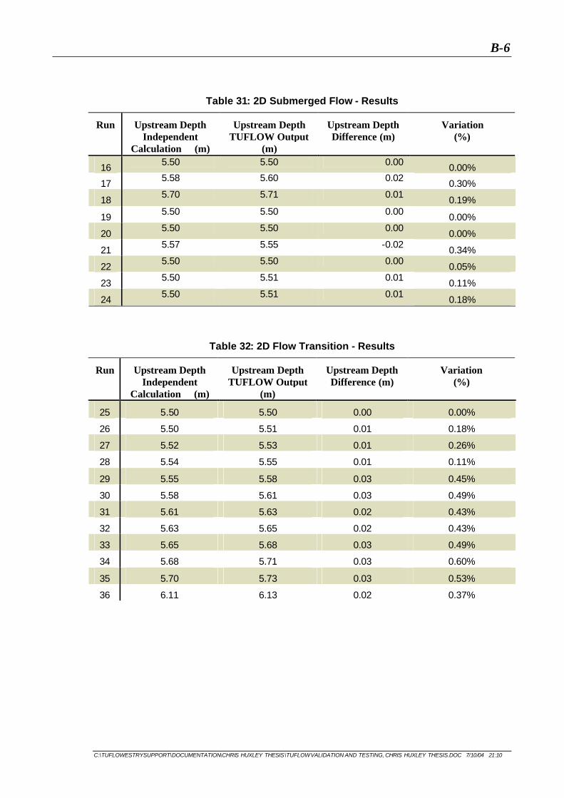
B-6
C:\TUFLOWESTRYSUPPORT\DOCUMENTATION\CHRIS HUXLEY THESIS\TUFLOW VALIDATION AND TESTING, CHRIS HUXLEY THESIS.DOC 7/10/04 21:10
Table 31: 2D Submerged Flow - Results
Run Upstream Depth Independent
Calculation (m)
Upstream Depth TUFLOW Output
(m)
Upstream Depth Difference (m)
Variation (%)
16 5.50 5.50 0.00 0.00%
17 5.58 5.60 0.02 0.30%
18 5.70 5.71 0.01 0.19%
19 5.50 5.50 0.00 0.00%
20 5.50 5.50 0.00 0.00%
21 5.57 5.55 -0.02 0.34%
22 5.50 5.50 0.00 0.05%
23 5.50 5.51 0.01 0.11%
24 5.50 5.51 0.01 0.18%
Table 32: 2D Flow Transition - Results
Run Upstream Depth Independent
Calculation (m)
Upstream Depth TUFLOW Output
(m)
Upstream Depth Difference (m)
Variation (%)
25 5.50 5.50 0.00 0.00%
26 5.50 5.51 0.01 0.18%
27 5.52 5.53 0.01 0.26%
28 5.54 5.55 0.01 0.11%
29 5.55 5.58 0.03 0.45%
30 5.58 5.61 0.03 0.49%
31 5.61 5.63 0.02 0.43%
32 5.63 5.65 0.02 0.43%
33 5.65 5.68 0.03 0.49%
34 5.68 5.71 0.03 0.60%
35 5.70 5.73 0.03 0.53%
36 6.11 6.13 0.02 0.37%

C-7
C:\TUFLOWESTRYSUPPORT\DOCUMENTATION\CHRIS HUXLEY THESIS\TUFLOW VALIDATION AND TESTING, CHRIS HUXLEY THESIS.DOC 7/10/04 21:10
APPENDIX C: OPEN CHANNEL FLOW
2D Channel Results Table 33: 2D Channel Flow Results – Slope = 10.4%
Run Depth Independent
Calculations (m)
Depth TUFLOW Output
(m)
Depth Difference (m)
Variation (%)
1 0.125 0.124 -0.001 0.300%
2 0.189 0.188 -0.001 0.424%
3 0.241 0.240 -0.001 0.361%
4 0.286 0.285 -0.001 0.460%
5 0.327 0.329 0.002 0.485%
6 0.365 0.364 -0.001 0.333%
7 0.189 0.189 0.000 0.211%
8 0.286 0.287 0.001 0.203%
9 0.365 0.364 -0.001 0.278%
10 0.434 0.435 0.001 0.166%
11 0.497 0.495 -0.002 0.327%
12 0.554 0.555 0.001 0.151%
13 0.241 0.240 -0.001 0.361%
14 0.365 0.365 0.000 0.087%
15 0.466 0.467 0.001 0.076%
16 0.554 0.555 0.001 0.151%
17 0.634 0.635 0.001 0.199%
18 0.707 0.705 -0.002 0.306%
Table 34: 2D Channel Flow Results – Slope = 5.2%
Run Depth Independent
Calculations (m)
Depth TUFLOW Output
(m)
Depth Difference (m)
Variation (%)
19 0.153 0.154 0.001 0.439%
20 0.232 0.233 0.001 0.216%
21 0.297 0.298 0.001 0.459%
22 0.353 0.352 -0.001 0.174%
23 0.403 0.404 0.001 0.192%
24 0.450 0.452 0.002 0.458%
25 0.232 0.233 0.001 0.216%

C-8
C:\TUFLOWESTRYSUPPORT\DOCUMENTATION\CHRIS HUXLEY THESIS\TUFLOW VALIDATION AND TESTING, CHRIS HUXLEY THESIS.DOC 7/10/04 21:10
26 0.353 0.353 0.000 0.110%
27 0.450 0.451 0.001 0.237%
28 0.535 0.536 0.001 0.209%
29 0.612 0.610 -0.002 0.276%
30 0.683 0.684 0.001 0.210%
31 0.297 0.296 -0.001 0.213%
32 0.450 0.451 0.001 0.237%
33 0.574 0.575 0.001 0.150%
34 0.683 0.685 0.002 0.356%
35 0.781 0.783 0.002 0.309%
Table 35: 2D Channel Flow Results – Slope = 2.6%
Run Depth Independent
Calculations (m)
Depth TUFLOW Output
(m)
Depth Difference (m)
Variation (%)
37 0.189 0.189 0.000 0.105%
38 0.286 0.286 0.000 0.111%
39 0.365 0.366 0.001 0.159%
40 0.434 0.435 0.001 0.166%
41 0.497 0.496 -0.001 0.126%
42 0.554 0.552 -0.002 0.390%
43 0.286 0.286 0.000 0.251%
44 0.434 0.435 0.001 0.166%
45 0.554 0.553 -0.001 0.210%
46 0.659 0.660 0.001 0.180%
47 0.753 0.751 -0.002 0.321%
48 0.841 0.842 0.001 0.152%
49 0.365 0.365 0.000 0.224%
50 0.554 0.556 0.002 0.241%
51 0.707 0.709 0.002 0.259%
52 0.841 0.842 0.001 0.152%
53 0.961 0.960 -0.001 0.149%

C-9
C:\TUFLOWESTRYSUPPORT\DOCUMENTATION\CHRIS HUXLEY THESIS\TUFLOW VALIDATION AND TESTING, CHRIS HUXLEY THESIS.DOC 7/10/04 21:10
Table 36: 2D Channel Flow Results – Slope = 1.3%
Run Depth Independent
Calculations (m)
Depth TUFLOW Output
(m)
Depth Difference (m)
Variation (%)
55 0.232 0.232 0.000 0.214%
56 0.353 0.354 0.001 0.251%
57 0.450 0.449 -0.001 0.318%
58 0.535 0.535 0.000 0.022%
59 0.612 0.613 0.001 0.214%
60 0.683 0.684 0.001 0.210%
61 0.353 0.354 0.001 0.251%
62 0.535 0.536 0.001 0.209%
63 0.683 0.685 0.002 0.356%
64 0.811 0.811 0.000 0.057%
65 0.928 0.930 0.002 0.217%
66 1.035 1.035 0.000 0.047%
67 0.450 0.450 0.000 0.016%
68 0.683 0.685 0.002 0.356%
69 0.871 0.870 -0.001 0.117%
70 1.035 1.035 0.000 0.047%
71 1.184 1.185 0.001 0.076%
72 1.321 1.325 0.004 0.290%
Table 37: 2D Channel Flow Results – Slope = 0.2%
Run Depth Independent
Calculations (m)
Depth TUFLOW Output
(m)
Depth Difference (m)
Variation (%)
73 0.408 0.408 0.000 0.001%
74 0.619 0.620 0.001 0.171%
75 0.790 0.790 0.000 0.021%
76 0.939 0.940 0.001 0.107%
77 1.074 1.070 -0.004 0.353%
78 1.198 1.200 0.002 0.155%
79 0.619 0.620 0.001 0.171%
80 0.939 0.940 0.001 0.107%
81 1.198 1.200 0.002 0.155%
82 1.424 1.425 0.001 0.062%

C-10
C:\TUFLOWESTRYSUPPORT\DOCUMENTATION\CHRIS HUXLEY THESIS\TUFLOW VALIDATION AND TESTING, CHRIS HUXLEY THESIS.DOC 7/10/04 21:10
83 1.628 1.623 -0.005 0.318%
84 1.816 1.810 -0.006 0.341%
85 0.790 0.790 0.000 0.021%
86 1.198 1.200 0.002 0.155%
87 1.528 1.530 0.002 0.102%
88 1.816 1.815 -0.001 0.066%
89 2.076 2.080 0.004 0.204%
90 2.315 2.320 0.005 0.230%
Table 38: 2D Channel Flow Results – Slope = 0.02%
Run Depth Independent
Calculations (m)
Depth TUFLOW Output
(m)
Depth Difference (m)
Variation (%)
91 0.815 0.818 0.003 0.274%
92 1.189 1.190 0.001 0.066%
93 1.578 1.580 0.002 0.157%
94 1.874 1.880 0.006 0.297%
95 2.142 2.140 -0.002 0.101%
96 2.389 2.385 -0.004 0.150%
97 1.237 1.233 -0.004 0.296%
98 1.874 1.870 -0.004 0.236%
99 2.389 2.380 -0.009 0.360%
100 2.835 2.840 0.005 0.179%
101 3.236 3.240 0.004 0.121%
102 3.604 3.600 -0.004 0.114%
103 1.578 1.573 -0.005 0.287%
104 2.389 2.380 -0.009 0.360%
105 3.040 3.050 0.010 0.320%
106 3.604 3.600 -0.004 0.114%
107 4.109 4.100 -0.009 0.229%
108 4.572 4.580 0.008 0.181%

C-11
C:\TUFLOWESTRYSUPPORT\DOCUMENTATION\CHRIS HUXLEY THESIS\TUFLOW VALIDATION AND TESTING, CHRIS HUXLEY THESIS.DOC 7/10/04 21:10
Floodplain Results Table 39: 2D Floodplain Flow Results – Slope = 10.4%
Run Depth Independent
Calculations (m)
Depth TUFLOW Output
(m)
Depth Difference (m)
Variation (%)
1 0.148 0.149 0.001 0.686%
2 0.224 0.226 0.002 0.715%
3 0.286 0.289 0.003 0.942%
4 0.340 0.343 0.003 0.784%
5 0.389 0.392 0.003 0.723%
6 0.434 0.438 0.004 0.855%
7 0.224 0.226 0.002 0.715%
8 0.340 0.343 0.003 0.784%
9 0.434 0.438 0.004 0.855%
10 0.516 0.520 0.004 0.712%
11 0.590 0.595 0.005 0.757%
12 0.659 0.664 0.005 0.754%
13 0.286 0.289 0.003 0.942%
14 0.434 0.438 0.004 0.855%
15 0.554 0.559 0.005 0.856%
16 0.659 0.664 0.005 0.754%
17 0.754 0.759 0.005 0.688%
18 0.841 0.847 0.006 0.672%
Table 40: 2D Floodplain Flow Results – Slope = 5.2%
Run Depth Independent
Calculations (m)
Depth TUFLOW
Output (m)
Depth Difference (m)
Variation (%)
19 0.353 0.354 0.001 0.403%
20 0.419 0.421 0.002 0.440%
21 0.479 0.482 0.003 0.550%
22 0.535 0.537 0.002 0.388%
23 0.276 0.275 -0.001 0.479%
24 0.419 0.417 -0.002 0.512%
25 0.535 0.532 -0.003 0.546%
26 0.636 0.633 -0.003 0.478%

C-12
C:\TUFLOWESTRYSUPPORT\DOCUMENTATION\CHRIS HUXLEY THESIS\TUFLOW VALIDATION AND TESTING, CHRIS HUXLEY THESIS.DOC 7/10/04 21:10
27 0.728 0.724 -0.004 0.483%
28 0.812 0.808 -0.004 0.489%
29 0.353 0.351 -0.002 0.446%
30 0.535 0.532 -0.003 0.546%
31 0.683 0.680 -0.003 0.481%
32 0.812 0.809 -0.003 0.366%
33 0.929 0.924 -0.005 0.524%
34 1.037 1.032 -0.005 0.467%
35 0.229 0.227 -0.002 0.979%
36 0.348 0.343 -0.005 1.351%
Table 41: 2D Floodplain Flow Results – Slope = 3.6%
Run Depth Independent
Calculations (m)
Depth TUFLOW
Output (m)
Depth Difference (m)
Variation (%)
37 0.444 0.438 -0.006 1.283%
38 0.528 0.533 0.005 1.027%
39 0.603 0.610 0.007 1.090%
40 0.673 0.680 0.007 0.977%
41 0.347 0.350 0.003 0.884%
42 0.527 0.533 0.006 1.137%
43 0.673 0.680 0.007 1.087%
44 0.800 0.808 0.008 1.005%
45 0.914 0.921 0.007 0.762%
46 1.020 1.030 0.010 0.949%
47 0.443 0.438 -0.005 1.058%
48 0.672 0.680 0.008 1.202%
49 0.858 0.868 0.010 1.183%
50 1.020 1.030 0.010 0.949%
51 1.167 1.155 -0.012 1.056%
52 1.303 1.315 0.012 0.896%
53 0.427 0.422 -0.005 1.195%
54 0.280 0.279 -0.001 0.494%

C-13
C:\TUFLOWESTRYSUPPORT\DOCUMENTATION\CHRIS HUXLEY THESIS\TUFLOW VALIDATION AND TESTING, CHRIS HUXLEY THESIS.DOC 7/10/04 21:10
Table 42: 2D Floodplain Flow Results – Slope = 1.3%
Run Depth Independent
Calculations (m)
Depth TUFLOW Output
(m)
Depth Difference (m)
Variation (%)
55 0.425 0.423 -0.002 0.546%
56 0.543 0.539 -0.004 0.703%
57 0.645 0.640 -0.005 0.844%
58 0.738 0.732 -0.006 0.851%
59 0.824 0.817 -0.007 0.852%
60 0.425 0.422 -0.003 0.781%
61 0.645 0.640 -0.005 0.844%
62 0.824 0.817 -0.007 0.852%
63 0.980 0.972 -0.008 0.826%
64 1.121 1.111 -0.010 0.924%
65 1.252 1.240 -0.012 0.949%
66 0.545 0.540 -0.005 0.933%
67 0.827 0.818 -0.009 1.145%
68 1.057 1.045 -0.012 1.107%
69 1.252 1.240 -0.012 0.949%
70 1.433 1.417 -0.016 1.091%
71 1.619 1.600 -0.019 1.160%
72 0.492 0.489 -0.003 0.659%
Table 43: 2D Floodplain Flow Results – Slope = 0.2%
Run Depth Independent
Calculations (m)
Depth TUFLOW Output
(m)
Depth Difference (m)
Variation (%)
73 0.747 0.742 -0.005 0.689%
74 0.954 0.945 -0.009 0.944%
75 1.135 1.127 -0.008 0.692%
76 1.299 1.289 -0.010 0.739%
77 1.450 1.436 -0.014 0.958%
78 0.747 0.741 -0.006 0.823%
79 1.135 1.125 -0.010 0.868%
80 1.450 1.440 -0.010 0.683%
81 1.726 1.712 -0.014 0.790%
82 1.975 1.955 -0.020 1.038%

C-14
C:\TUFLOWESTRYSUPPORT\DOCUMENTATION\CHRIS HUXLEY THESIS\TUFLOW VALIDATION AND TESTING, CHRIS HUXLEY THESIS.DOC 7/10/04 21:10
83 2.207 2.180 -0.027 1.205%
84 0.954 0.960 0.006 0.625%
85 1.450 1.458 0.008 0.556%
86 1.853 1.840 -0.013 0.716%
87 2.194 2.180 -0.014 0.643%
88 2.513 2.490 -0.023 0.904%
89 2.808 2.781 -0.027 0.947%
90 3.427 3.390 -0.037 1.071%
Table 44: 2D Floodplain Flow Results – Slope = 0.02%
Run Depth Independent
Calculations (m)
Depth TUFLOW
Output (m)
Depth Difference (m)
Variation (%)
91 0.988 0.976 -0.012 1.177%
92 1.481 1.465 -0.016 1.079%
93 1.893 1.870 -0.023 1.219%
94 2.254 2.230 -0.024 1.069%
95 2.582 2.550 -0.032 1.221%
96 2.885 2.855 -0.030 1.026%
97 1.481 1.469 -0.012 0.809%
98 2.241 2.220 -0.021 0.918%
99 2.867 2.840 -0.027 0.949%
100 3.427 3.390 -0.037 1.071%
101 3.941 3.900 -0.041 1.042%
102 4.407 4.360 -0.047 1.074%
103 1.893 1.880 -0.013 0.691%
104 2.838 2.820 -0.018 0.635%
105 3.635 3.610 -0.025 0.685%
106 4.336 4.290 -0.046 1.050%
107 4.973 4.906 -0.067 1.348%
108 5.565 5.500 -0.065 1.164%

C-15
C:\TUFLOWESTRYSUPPORT\DOCUMENTATION\CHRIS HUXLEY THESIS\TUFLOW VALIDATION AND TESTING, CHRIS HUXLEY THESIS.DOC 7/10/04 21:10
2D Flooplain/2D Channel Results Table 45: 2D Floodplain/2D Channel Flow Results – Slope = 1.3%
Run Depth Independent
Calculations (m)
Depth TUFLOW
Output (m)
Depth Difference
(m)
Variation (%)
1 3.133 3.130 -0.003 0.097%
2 3.133 3.130 -0.003 0.097%
3 3.133 3.130 -0.003 0.097%
4 3.133 3.130 -0.003 0.097%
5 3.133 3.130 -0.003 0.097%
6 3.133 3.130 -0.003 0.097%
7 4.257 4.250 -0.007 0.157%
8 4.257 4.250 -0.007 0.157%
9 4.257 4.250 -0.007 0.157%
10 4.257 4.250 -0.007 0.157%
11 4.257 4.250 -0.007 0.157%
12 4.257 4.250 -0.007 0.157%
13 5.480 5.420 -0.060 1.104%
14 5.654 5.590 -0.064 1.135%
15 5.767 5.700 -0.067 1.170%
16 5.850 5.780 -0.070 1.201%
17 5.914 5.845 -0.069 1.173%
18 5.966 5.900 -0.066 1.106%
Table 46: 2D Floodplain/2D Channel Flow Results – Slope = 0.02%
Run Depth Independent
Calculations (m)
Depth TUFLOW Output
(m)
Depth Difference (m)
Variation (%)
19 6.728 6.680 -0.048 0.719%
20 7.465 7.420 -0.045 0.600%
21 7.989 7.930 -0.059 0.738%
22 8.398 8.340 -0.058 0.693%
23 8.733 8.680 -0.053 0.603%
24 9.014 8.970 -0.044 0.488%
25 7.541 7.480 -0.061 0.807%
26 8.654 8.587 -0.067 0.773%

C-16
C:\TUFLOWESTRYSUPPORT\DOCUMENTATION\CHRIS HUXLEY THESIS\TUFLOW VALIDATION AND TESTING, CHRIS HUXLEY THESIS.DOC 7/10/04 21:10
27 9.458 9.382 -0.076 0.803%
28 10.092 10.035 -0.057 0.569%
29 10.616 10.560 -0.056 0.524%
30 11.059 11.000 -0.059 0.534%
31 8.520 8.470 -0.050 0.589%
32 10.090 10.024 -0.066 0.657%
33 11.235 11.160 -0.075 0.669%
34 12.145 12.080 -0.065 0.534%
35 12.899 12.843 -0.056 0.436%
36 13.542 13.491 -0.051 0.374%
2D Flooplain/1D Channel Results
Table 47: 2D Floodplain/1D Channel Flow Results – Slope = 1.3%
Run Depth Independent Calculations (m)
Depth TUFLOW Output (m)
Depth Difference (m)
Variation (%)
1 3.133 3.130 -0.003 0.097%
2 3.133 3.130 -0.003 0.097%
3 3.133 3.130 -0.003 0.097%
4 3.133 3.130 -0.003 0.097%
5 3.133 3.130 -0.003 0.097%
6 3.133 3.130 -0.003 0.097%
7 4.257 4.250 -0.007 0.157%
8 4.257 4.250 -0.007 0.157%
9 4.257 4.250 -0.007 0.157%
10 4.257 4.250 -0.007 0.157%
11 4.257 4.250 -0.007 0.157%
12 4.257 4.250 -0.007 0.157%
13 5.480 5.450 -0.030 0.556%
14 5.654 5.620 -0.034 0.604%
15 5.767 5.730 -0.037 0.650%
16 5.850 5.822 -0.028 0.483%
17 5.914 5.945 0.031 0.515%
18 5.966 5.990 0.024 0.401%

C-17
C:\TUFLOWESTRYSUPPORT\DOCUMENTATION\CHRIS HUXLEY THESIS\TUFLOW VALIDATION AND TESTING, CHRIS HUXLEY THESIS.DOC 7/10/04 21:10
Table 48: 2D Floodplain/1D Channel Flow Results – Slope = 0.02%
Run Depth Independent
Calculations (m)
Depth TUFLOW Output
(m)
Depth Difference (m)
Variation (%)
19 6.728 6.770 0.042 0.615%
20 7.465 7.510 0.045 0.602%
21 7.989 8.020 0.031 0.387%
22 8.398 8.430 0.032 0.377%
23 8.733 8.760 0.027 0.312%
24 9.014 9.040 0.026 0.288%
25 7.541 7.600 0.059 0.779%
26 8.654 8.710 0.056 0.644%
27 9.458 9.500 0.042 0.443%
28 10.092 10.140 0.048 0.469%
29 10.616 10.660 0.044 0.416%
30 11.059 11.110 0.051 0.459%
31 8.520 8.580 0.060 0.697%
32 10.090 10.140 0.050 0.490%
33 11.235 11.180 -0.055 0.491%
34 12.145 12.190 0.045 0.370%
35 12.899 12.950 0.051 0.391%
36 13.542 13.590 0.048 0.356%

C-18
C:\TUFLOWESTRYSUPPORT\DOCUMENTATION\CHRIS HUXLEY THESIS\TUFLOW VALIDATION AND TESTING, CHRIS HUXLEY THESIS.DOC 7/10/04 21:10
8 REFERENCES
AUSTROADS. (1994) “Waterway Design. A Guide to the hydraulic design of bridges, culverts and
floodway”, AUSTROADS
Barton, C.L. (2001), “Flow Through an Abrupt Constriction – 2D Hydrodynamic Model
Performance and Influence of spatial Resolution”, Cathie Louise Barton, M.ENG.Sc Master
Bradley, J.N. (1978), ”Hydraulics of Bridge Waterways”, US Department of Transport.
Benham, S. and Rogencamp, G. (2003), “Application of 2D Flood Models with 1D Drainage
Elements”, Forbes Conference 2003.
CPAA. (1991), “Hydraulics of Precast Concrete Conduits”, Concrete Pipe Association of
Australiasia.
Chanson, H. (1999), “The Hydraulics of Open Channel Flow – An Introduction”, Butterworth,
Heinmann.
Chow, V.T. (1973), Open Channel Hydraulics, McGraw Hill book Company Inc.
DHI, (1998), ”MIKE21 Users Manual”, DHI.
DHI, (1999), ”MIKE11 Users Manual”, DHI.
FHA, “Finite Element surfacewater Modelling System Two Dimensional Flow in a horizontal Plane,
Version 2 Users Manual”, US Department of Transport, Federal Highways
Finnemore, J.E., and Franzini, J.B. (2002), “Fluid Mechanics”, McGraw Hill book Company Inc.
Hamill, L. (1995), “Understanding Hydraulics”, MacMillan Press Ltd.
Hager, W.H., and Schwalt, M. (1994), “Broad Crested Weir”, Journal of Irrigation and Drainage
Engineering, 120(1) pp13-26.
Hardy, R.J., Bates, P.D., and Anderson, M.G. (1999), “The importance of special resolution in
hydraulic models for floodplain environments”, Journal of Hydrology 216 pp124-136
Henderson, F.M. (1966), “Open channel Flow”, MacMillan Publishing Co.
King, I.P. (1998), “RMA-2 Users manual”, Department of Civil Engineering California

C-19
C:\TUFLOWESTRYSUPPORT\DOCUMENTATION\CHRIS HUXLEY THESIS\TUFLOW VALIDATION AND TESTING, CHRIS HUXLEY THESIS.DOC 7/10/04 21:10
Kutijar, V. & Hewett, C. (2002), “Modelling of Supercritical Flow Conditions Revisited”, Journal of Hydraulic Research 20(2) pp145-152
Leopardi, A., Oliveri, E. & Greco. M. (2002), “Two-Dimensional Modeling of Floods to Map Risk-Prone Areas”, Journal of Water Resources Planning and Management, 128(3) pp. 168-178.
McCutcheon, S.C. (1989), “Water quality Modelling, vol.1, transport and surface Exchange in
Rivers”, CRC, Boca Raton, FL.
Martin, J.L. and McCutcheon, S.C. (1999), “Hydrodynamics and Transport for Water quality
Modeling”, CRC Press
Mynett, A.E. (1999), “Hydroinformatics and its applications at Delft Hydraulics”, Journal of
Hydroinformatics, 01(2), pp 83-102.
NCSA. (1998), “Scaling and Performance of a 3D Radiation Hydrodynamics Code on Message-
Passing Parallel Computers”, National Center for Supercomputing Applications
Rogencamp, G. & Syme, W.J. (2003), “Application of 2D/1D Hydraulic Models in steep to flat
urban catchments”, The Institution of Engineers, Australia 28th International Hydrology and Water
Resources Symposium Wollongong, NSW 10 - 14 November 2003.
Streeter, V.L. (1962), “Fluid Mechanics”, McGraw Hill book Company Inc
Syme, W.J. (1991), “Dynamically Linked Two dimensional /One dimensional Hydrodynamic
Modelling Program for Rivers, Esturies and Coastal Waters”, William Syme, M.ENG.Sc (Research)
Thesis, University of Queensland.
Syme, W.J. (2001), “Modelling of Bends and Hydraulic Structures in a Two-Dimensional Scheme”,
The Institution of Engineers, Australia Conference on Hydraulics in Civil Engineering Hobart 28 –30
November 2001.
WBM Pty Ltd. (1998), “ESTRY Users Manual”, WBM Oceanics Australia.
WBM Pty Ltd. (2003), TUFLOW –An Introduction to TUFLOW”, WBM Oceanics Australia.
WBM Pty Ltd. (2004), “TUFLOW Users Manual”, WBM Oceanics Australia.
Zoppou, C. and Roberts, S. (2000), “Robust and efficient solution of the 2D Shallow Water
Equation with domains containing dry beds”, Australian Mathematical Society
Related Documents


