Tucker McElroy and Scott Holan Statistical Research ... REPORT SERIES (Statistics #2005-10) A Nonparametric Test for Assessing Spectral Peaks Tucker McElroy and Scott Holan 1 Statistical

RESEARCH REPORT SERIES(Statistics #2005-10)

A Nonparametric Test for Assessing Spectral Peaks

Tucker McElroy and Scott Holan1

Statistical Research DivisionU.S. Bureau of the CensusWashington D.C. 20233

Department of Statistics, University of Missouri-Columbia, 146 Middlebush Hall, Columbia, MO, 65211-6100,1

holans @missouri,edu

Report issued: December 20, 2005

Disclaimer: This report is released to inform interested parties of research and to encourage discussion. The views

expressed are those of the authors and not necessarily those of the U.S. Census Bureau.

A Nonparametric Test for Assessing Spectral Peaks

Tucker McElroy∗and Scott Holan†

U.S. Census Bureau and University of Missouri-Columbia

Abstract

Peaks in the spectrum of a stationary process are indicative of the presence of a periodic phe-

nomenon, such as a seasonal effect or business cycle. This work proposes to measure and test for

the presence of such spectral peaks via assessing their aggregate acceleration and velocity. Our

method is developed nonparametrically, and thus may be useful in a preliminary analysis of a

series. The technique is also useful for detecting the presence of residual seasonality in seasonally

adjusted data. The diagnostic is investigated through simulation and two data examples.

Keywords. Seasonal Adjustment, Spectral Density, Nonparametric Kernel Methods.

Disclaimer This paper is released to inform interested parties of ongoing research and to encour-

age discussion of work in progress. The views expressed are those of the authors and not necessarily

those of the U.S. Census Bureau.

1 Introduction

The presence of a peak in the spectrum of a stationary process is indicative of a periodic phe-

nomenon, such as a seasonal effect or business cycle. There is a widespread interest in the identifica-

tion of such peaks in the engineering and econometrics literature, since a pronounced spectral node

will exert a potent influence on the dynamics of the stochastic process. A peak may indicate the

presence of auto-regressive behavior, or even nonstationarity in the extreme case. If the strength of

the peak, assessed through its height and width relative to neighboring values, is sufficiently signif-

icant, any model of the dynamics that ignores the corresponding periodicities will be misspecified.

In both engineering and econometrics, one may be interested in signal extraction or forecasting,

both of which are sensitive to the presence of spectral peaks.∗Statistical Research Division, U.S. Census Bureau, 4700 Silver Hill Road, Washington, D.C. 20233-9100,

[email protected]†Department of Statistics, University of Missouri-Columbia, 146 Middlebush Hall, Columbia, MO, 65211-6100,

[email protected]

1

Today, much of time series modelling is performed in the time domain, often utilizing popular

ARIMA models (Box and Jenkins, 1976). The ARIMA model stipulates a rational function for the

pseudo-spectral density, and thus peaks will be automatically identified. The increasingly popular

Unobserved Components (UC) approach to modelling econometric time series stipulates a separate

unobserved time series for each significant dynamic of the data; alternatively, one may often view

each component as a time series that contributes to a certain band of the spectrum. For example,

the popular trend-cycle UC model for econometric data has a low-frequency component (the trend)

and a higher-frequency component (the cycle), which in Hodrick-Prescott (1997) occupies the high

frequency band, but may also be viewed as the upper portion of the low frequency band – see

Harvey and Trimbur (2003). The models for these components typically have a peak in the cor-

responding spectrum. Another example from econometrics is provided by raw seasonal time series

data encountered at federal agencies such as the U.S. Census Bureau and U.S. Bureau of Labor

Statistics. A UC model for a monthly series would include trend and seasonal, where the latter

is characterized by pseudo-spectrum with peaks at the frequencies π/6, 2π/6, 3π/6, 4π/6, 5π/6,

and 6π/6 (Findley, Monsell, Bell, Otto, and Chen, 1998). In addition, the presence of trading day

effects result in spectral peaks at .348 and .432 cycles per month (Cleveland and Devlin, 1980),

which would typically be removed through regression.

Although these spectral modelling considerations are also of interest to engineers, the identifi-

cation of spectral peaks is valuable for other applications (Percival and Walden, 1993; Priestley,

1981). For example, the detection of a signal in ambient noise is important in environments such

as communications, radar, and active sonar (Haykin, 1996). The conventional detector is merely

given by comparing the height of the periodogram at a desired frequency to a pre-specified thresh-

old. The adaptive line enhancer of Widrow, McCool, and Ball (1975) first applies a filter to the

data, which can be viewed as a crude nonparametric signal extraction filter. Pre-filtering scales the

periodogram by the filter’s squared gain, which may attenuate neighboring values so as to deliver a

clearer picture of the spectrum in the desired range. This should not be confused with the kernel-

smoothing literature, which convolves a smoothing kernel with the periodogram, typically in such

a way that the kernel bandwidth shrinks with increasing sample size (Parzen, 1957a, 1957b). The

methodology of this paper is closely related to the pre-filtering approach.

A final application lies in the arena of federal statistics. Peak identification is important in

seasonal adjustment, since the presence of seasonal peaks in adjusted data may indicate inadequacy

of the signal extraction filters (Findley et al., 1998). In Soukup and Findley (1999), peaks are

identified through the concept of “visual significance,” a comparison of the height of an AR spectrum

estimator to neighboring values.

2

The paper at hand adopts a novel nonparametric strategy for the identification of spectral peaks.

Viewing the true spectral density as a smooth function (this can be quantified through sufficiently

rapid decay of the autocovariance function) f(λ), a peak is a frequency λ0 such that

f(λ0) = 0 f(λ0) < 0, (1)

where f and f denote first and second derivatives. Clearly, the acceleration must be negative with

some significance in order for the concept to be meaningful. Upon further reflection, it seems that

examining the infinitesimal geometry of f at the single point λ0 is naıve, since any small spike in the

side of an increasing function may satisfy (1) while being dissociated from more intuitive notions

of what constitutes a peak. Therefore, we must have negative acceleration in a reasonably large

neighborhood of λ0. This thinking leads to the diagnostic of this paper: an aggregate measure of

acceleration of the spectral density, with appropriate statistical normalization. Mathematically, this

will take the form of a kernel-smoothed periodogram, but without the bandwidth being dependent

on sample size. In Section Two we develop the mathematical ideas of this method, illustrated

through two carefully chosen choices of kernels. Section Three presents a theoretical study of our

diagnostics, providing a central limit theorem that allows for hypothesis testing. The methodology

is tested in Section Four; simulations provide a finite sample description of the size and power of

our test. We further demonstrate the utility of our methods through two examples: cycle detection

in U.S. GDP and detection of residual seasonality in seasonally adjusted U.S. Retail Sales of Shoe

Stores. Section Five concludes.

2 Method

Suppose that, after suitable transformations and differencing if necessary, we have a mean

zero stationary time series X1, X2, · · · , Xn, which will sometimes be denoted by the vector X =

(X1, X2, · · · , Xn)′. The spectral density f(λ) is well-defined so long as the autocovariance function

γf (h) is summable, and is given by

f(λ) =∞∑

h=−∞γf (h)e−ihλ (2)

with i =√−1 and λ ∈ [−π, π]. It follows that the inverse fourier transform yields

γf (h) =12π

∫ π

−πf(λ)eihλ dλ,

a relation that we will use repeatedly in the sequel. This relationship between γg and g holds for

any integrable function g. Furthermore, denoting the Toeplitz matrix associated with γg by Σ(g),

it follows that

Σjk(g) =12π

∫ π

−πg(λ)ei(j−k)λdλ.

3

Now from (2), f is d times continuously differentiable if

∞∑

h=−∞|h|d|γf (h)| < ∞.

We assume that f is twice continuously differentiable for the remainder of the paper (this space of

functions will be abbreviated as C2).

We now define the notion of aggregate acceleration of the spectral density. Given a kernel A ∈ C1,

the functional12π

∫ π

−πA(λ)f(λ)dλ (3)

forms an aggregate measure of acceleration; this is only sensible under some conditions on the kernel

A. Intuitively, the most obvious kernel would be an indicator function on an interval centered at

the peak frequency λ0. However, it will be advantageous mathematically to use a smoother kernel.

Below, we list several desirable properties of the kernel as an aggregate measure of acceleration at

frequency λ0 = 0.

1. A is an even function

2. A is higher at frequency zero, and tapers off at high frequencies

3. A(±π) = 0

4. A(±π) = 0

5.∫ π−π A(λ)dλ = 1

Condition 1 is reasonable since f is also even. Since the functional (3) essentially computes an

expectation under the measure A(λ)dλ, condition 2 stipulates that the mass is centered at the

frequency of interest, namely λ0. Conditions 3 and 4 arise from mathematical considerations, but

also ensure that the kernel tapers down smoothly to zero on the boundaries. Condition 5 normalizes

the kernel so that (3) does not distort the overall scale. Now due to conditions 3 and 4, we can

integrate (3) by parts twice, and obtain

12π

∫ π

−πA(λ)f(λ)dλ

exactly (note that A is allowed to have jump discontinuities, since A ∈ C1). We propose a statistical

estimate of the above measure of acceleration, given as follows. Note that the quadratic form

1n

X′Σ(g)X =

12π

∫ π

−πg(λ)In(λ)dλ,

4

where I denotes the periodogram. We define it at a continuous spectrum of frequencies as follows

I(λ) =1n

∣∣∣∣∣n∑

t=1

Xte−itλ

∣∣∣∣∣2

=n−1∑

h=1−n

R(h)e−ihλ,

with R(h) equal to the sample (uncentered) autocovariance function. Therefore, an estimate of (3)

is obtained by applying a “method of moments” plug-in approach, and is given by

Qn =1n

X′Σ(A)X.

Note that the inconsistency of the periodogram is resolved by the spectral aggregation A(λ)dλ, as

will be demonstrated in the next section. By itself, Qn is not useful, since we do not know the scale

of the statistic. It will be demonstrated in the next section that a reasonable estimate of scale is

provided by the square root of

Sn = R′Σ(A2)R,

where R = {R(1− n), · · · , R(0), · · · , R(n− 1)}′ (we take the square of the second derivative above).

Although having a normalized estimate of the aggregate acceleration is of some interest, our

primary goal is to test against a null that there is no peak, in favor of establishing (with significance)

the presence of a peak. To that end, consider the following hypotheses

H0 :12π

∫ π

−πA(λ)f(λ)dλ = 0

H1 :12π

∫ π

−πA(λ)f(λ)dλ < 0.

Since the alternative is lower one-sided, this tests for negative acceleration, which is appropriate for

a spectral peak (if trough detection is desired, simply reverse the sign). Then under H0 and some

mild conditions on the stochastic process,√

nQn/√

Sn is asymptotically normal (this is proved in

the following section).

Next, it is desirable to extend this methodology to λ0 6= 0. Therefore, consider an interval

[µ−β/2, µ+β/2] ⊂ [0, π], with µ typically chosen equal to λ0, and β chosen to distinguish between

local and global behavior (more on this later). We then define a modified kernel Aβ,µ that is a

shifted, scaled, and reflected version of the original kernel:

Aβ,µ(λ) =

πβ A

(2πβ (λ− µ)

), ifλ ∈ [µ− β/2, µ + β/2];

πβ A

(2πβ (λ + µ)

), ifλ ∈ [−µ− β/2,−µ + β/2];

0 else.

We remark that is is critical that β ≤ 2µ in this formulation. For this reason, extremely low and

high values of λ0 require a small β value, and λ0 equal to 0 or π cannot be tested at all. That is,

5

there is no way to determine whether there is a peak at these frequencies, since we can only observe

one side of the interval. Now the factor of π/β guarantees that condition 5 holds for Aβ,µ as well.

Conditions 2 and 3 become the statement that Aβ,µ and its derivative are zero at ±µ ± β/2. As

for condition 1, Aβ,µ is still even, but each portion is symmetric about ±µ. This symmetry will

guarantee that γAβ,µis real. Using a change of variables, we see that

γAβ,µ(h) = coshµγA(hβ/2π), (4)

so that the effect of β and µ are in some sense separable. Of course, we are ultimately interested

in Aβ,µ, which is given by

Aβ,µ(λ) =

4π3

β3 A(

2πβ (λ− µ)

), ifλ ∈ [µ− β/2, µ + β/2];

4π3

β3 A(

2πβ (λ + µ)

), ifλ ∈ [−µ− β/2,−µ + β/2];

0 else.

Assuming that [µ− β/2, µ + β/2] ⊂ [0, π], the square is given by

A2β,µ(λ) =

16π6

β6 A2(

2πβ (λ− µ)

), ifλ ∈ [µ− β/2, µ + β/2];

16π6

β6 A2(

2πβ (λ + µ)

), ifλ ∈ [−µ− β/2,−µ + β/2];

0 else.

From here, one can take the inverse Fourier Transform to construct Σ(Aβ,µ) and Σ(A2β,µ), as follows:

γAβ,µ(h) =

4π2

β2coshµγA(hβ/2π) (5)

γA2β,µ

(h) =16π5

β5coshµγA2(hβ/2π).

So what are some natural choices of kernel? In addition to the guidance offered by conditions one

through five, the inverse fourier transform of the kernel should be simple to compute. Certainly a

downward-facing quadratic has the right basic shape (condition 2), but cannot satisfy conditions

3, 4, and 5 all at once, as there are too many constraints. Below, we consider both a quartic and

the cosine curve, which obviously have the correct basic shape, and additionally are fairly simple

to transform.

2.1 Example 1: Quartic Kernel

Conditions 1 through 5 offer a number of constraints, which a simple quadratic cannot satisfy.

The next natural choice for a polynomial kernel is given by a quartic. Imposing all of the constraints

6

yields the following form:

A(λ) =158π4

(λ4 − 2π2λ2 + π4

)

A(λ) =158π4

(12λ2 − 4π2

).

Taking the inverse Fourier Transform of the acceleration yields

γA(h) =152π6

(π2 sinπh

h+

3π cosπh

h2− 3 sinπh

h3

),

to which we apply (5) and obtain

γAβ,µ(h) =

30β2π

coshµ

(sin k

k+

3 cos k

k2− 3 sin k

k3

),

where k = hβ/2. In a similar fashion, we obtain

γA2(h) =2254π11

(π4 sinπh

h+

6π3 cosπh

h2− 24π2 sinπh

h3− 54π cosπh

h4+

54 sinπh

h5

)

γA2β,µ

(h) =900β5π

coshµ

(sin k

k+

6 cos k

k2− 24 sin k

k3− 54 cos k

k4+

54 sin k

k5

)

with γA2β,µ

(0) = 180/(β5π). These formulas allow us to construct the appropriate Toeplitz matrices

for the diagnostic. Note that use of a sextic would allow for one free parameter, which would control

the shape of the kernel in some fashion.

2.2 Example 2: Sinusoidal Kernel

A similar shape to the quartic can be obtained through the use of a cosine function. The following

choice satisfies all the stated conditions on a kernel:

A(λ) =12π

(1 + cosλ)

A(λ) =12π

(− cosλ)

Taking the inverse Fourier Transform of the acceleration yields

γA(h) =−14π2

(sinπ(h + 1)

h + 1+

sinπ(h− 1)h− 1

),

to which we apply (5) and obtain

γAβ,µ(h) =

π

β2coshµ

(sin k

k + π+

sin k

k − π

),

where k = hβ/2. When k = ±π, we must replace the corresponding ratio by −1. For the squared

acceleration, we have:

γA2(h) =1

16π3

(2 sin πh

h+

sinπ(h + 2)h + 2

+sinπ(h− 2)

h− 2

)

γA2β,µ

(h) =π3

β5coshµ

(2 sin k

k+

sin k

k + 2π+

sin k

k − 2π

)

7

with γA2β,µ

(0) = 2π3/β5. These formulas allow us to construct the appropriate Toeplitz matrices

for the diagnostic. Note that they have a simpler form than the quartic.

3 Theory

In this section we derive asymptotic formulas for the diagnostics, which suggest a statistical nor-

malization that is appropriate for Gaussian data. These results are then applied to the hypothesis

testing paradigm, which facilitates testing and asymptotic power calculations.

3.1 Asymptotics

Some mild conditions on the data are required for the asymptotic theory; we follow the material

in Taniguchi and Kakizawa (2000, Section 3.1.1). Condition (B), due to Brillinger (1981), states

that the process is strictly stationary and condition (B1) of Taniguchi and Kakizawa (2000, page

55) holds. Condition (HT), due to Hosoya and Taniguchi (1982), states that the process has a

linear representation, and conditions (H1) through (H6) of Taniguchi and Kakizawa (2000, pages

55 – 56) hold. Neither of these conditions are stringent; for example, a causal MA(∞) process with

fourth moments satisfies (HT).

Theorem 1 Suppose that the process {Xt} satisfies either condition (B) or (HT), and the kernel

A satisfies the conditions of Section 2. Then

QnP−→ 1

2π

∫ π

−πA(λ)f(λ)dλ

as n →∞. Furthermore, √n

∫ π

−πA(λ) (In(λ)− f(λ)) dλ

is asymptotically normal with mean zero and variance

22π

∫ π

−πA2(λ)f2(λ) dλ +

1(2π)4

∫ π

−π

∫ π

−πA(λ)A(ω)GX(−λ, ω,−ω)dλdω

where GX is the tri-spectral density

GX(λ, ω, θ) =∞∑

j,k,l=−∞exp{−i(λj + ωk + θl)}cX(j, k, l).

The function cX denotes the fourth-order cumulant function.

Proof. Since A is real, even, and continuous, the result follows at once from Lemma 3.1.1 of

Taniguchi and Kakizawa (2000). Note that they define the periodogram with a 2π factor. 2

8

For Gaussian data, the second term in the variance vanishes, and we can estimate the first term

with12π

∫ π

−πA2(λ)I2

n(λ) dλ.

Note that this is essentially a plug-in estimate, substituting In for f , but we lose a factor of 2,

as the following result demonstrates. For assumptions on the data, we follow Chiu (1988), whose

results do not assume Gaussianity. Assumption 1 (8) of Chiu (1988) is a summability condition on

various higher order cumulants, which is satisfied, for example, by a Gaussian process with spectral

density in C2.

Theorem 2 Suppose that the process {Xt} satisfies Assumption 1 (8) of Chiu (1988), and the

kernel A satisfies the conditions of Section 2. Then

Sn =12π

∫ π

−πA2(λ)I2

n(λ)dλa.s.−→ 2

2π

∫ π

−πA2(λ)f2(λ)dλ

as n →∞.

Proof. Since A will be continuous in an interval (such as (µ− β/2, µ + β/2)), this result follows

directly from Corollary 1 of Chiu (1988), noting that they deal with the Riemann sums approx-

imation to the integral functional. Chiu (1988) also defines the periodogram with a 2π factor.

2

The computation of Sn is not immediately obvious, so we proceed as follows.

I2n(λ) = |In(λ)|2 =

n−1∑

h,k=1−n

R(h)R(k)ei(k−h)λ,

so applying A2(λ) and integrating yields

Sn =n−1∑

h,k=1−n

R(h)R(k)Σk,h(A2) = R′Σ(A2)R.

Now when the fourth order cumulants vanish, we can use Sn as a consistent estimate of the vari-

ance of Qn, and hence√

nQn/√

Sn should be asymptotically standard normal. By combining the

assumptions of Theorems 1 and 2, we arrive at the following result.

Theorem 3 Suppose that the fourth order cumulants of {Xt} vanish; that either condition (B)

or (HT) holds; and that Assumption 1 (8) of Chiu (1988) holds. Let the kernel A satisfy the

assumptions of Section 2. Then

√n

(Qn − 1

2π

∫ π−π A(λ)f(λ)dλ

)√

Sn

L=⇒ N (0, 1)

as n →∞.

9

Proof. Simply combine Theorems 1 and 2 with Slutsky’s Theorem (Bickel and Doksum, 1977).

2

Remark 1 The assumptions of the theorem are satisfied by Gaussian ARMA processes, for ex-

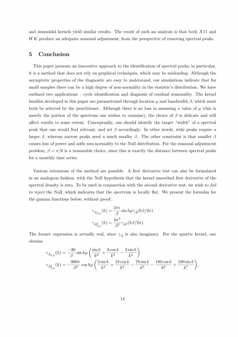
ample. Simulations indicate that the denominator Sn is slow to converge; its correlation with Qn

causes a degree of non-normality in smaller samples. Based on the qq-plot, there is close agreement

to the normal distribution, except at the right tail. Section 4 explores this behavior further through

simulation studies.

3.2 Applications

Under H0, the limiting mean value of the diagnostic is zero, and Theorem 3 indicates that√

nQn/√

Sn is asymptotically normal. Hence we develop critical values for the lower one-sided al-

ternative by using the standard normal distribution. Some simulation studies on the size properties

are discussed in the next section.

In order to calculate asymptotic power, we must formulate an appropriate element of the alter-

native space. Focusing on the case that we use a kernel Aβ,µ supported in a subset of the frequency

range, we can imagine spectral densities f that have a peak in that region. One way to think of

this, is to imagine that locally, the spectrum is given by an AR(2) of the form

(1− 2ρ cosωB + ρ2B2)Xt = εt

with white noise variance σ2, associated with some fixed frequency ω ∈ [0, π]. Then the spectrum

is

f(λ) =σ2

|1− 2ρ cosωe−iλ + ρ2e−2iλ|2,

which is maximized at λ0 = cos−1(cosω(1 + ρ2)/2ρ). Hence for a nonstationary AR(2) where

ρ = 1, ω is the mode of the infinite peak. Letting ρ, ω, and σ range as desired, the actual value of

θ = 12π

∫ π−π A(λ)f(λ)dλ can be computed (numerically), and the asymptotic power determined as

follows:

Prob(Type II Error) = Prob

(−zα/2 ≤

√n

Qn√Sn

≤ zα/2|H1

)

≈ Φ(zα/2 −√

nθ/√

Sn)− Φ(−zα/2 −√

nθ/√

Sn)

It is intuitive that power will be lost when the chosen µ does not match the maximum λ0. Likewise,

taking β too large or too small will detract from performance.

10

4 Empirical Work

Having developed the theoretical aspects of the spectral diagnostic, we now turn to its perfor-

mance in practice. We first present some results obtained from simulation, which provide insight

into the size and power properties of the test statistic. Then we investigate the utility of the diag-

nostic on two test examples: the first concerns the identification of a cycle peak in the spectrum,

and the second is concerned with identification of seasonal peaks in a seasonally adjusted series.

4.1 Simulation Studies

We simulated Gaussian white noise, which satisfies the assumptions of Theorem 3 as well as

providing θ = 12π

∫ π−π A(λ)f(λ)dλ = 0, so that H0 is true. Of course, there are many processes

other than white noise for which H0 is true – for example, any process with locally flat spectral

density. For simplicity of generation and exposition, we restrict ourselves to considering white

noise. For a (large) sample size of n = 360, using the quartic kernel with µ = π/6 and β = π/3

(this corresponds to a kernel centered on the interval [0, π/3]), a thousand repetitions yields an

empirical distribution of the normalized diagnostic with mean −0.01889724 and standard deviation

0.9213594. The sample quantile corresponding to the 5 percent level for the standard normal was

.056, giving close agreement to the nominal. Figure 1 displays the histogram, and Figure 2 displays

the qq-plot against the normal distribution. These results are not an artifact of the number of

draws, as they were unaffected by using more Monte Carlos.

Results were similar for other choices of µ and β; Tables 1 through 6 summarize size and power

properties as a function of β and sample size. In smaller samples we observed skewness in the

distribution (to the right or left depending on the choice of µ and β), which seems to be due to

correlation between Qn and Sn. The asymptotic normality of Qn becomes noticeable for much

smaller samples, but the use of Sn to estimate the size seems to alter the shape in small samples.

Experimentation with other estimates of Sn did not lead to any substantial improvements. One

approach to improving the shape is to change the testing paradigm to specific formulations of the

spectral density, e.g.,

H0 : f is constant on the interval [µ− β/2, µ + β/2].

Then, denoting the constant value by c, we compute

22π

∫ π

−πA2(λ)f2(λ)dλ = 2c2γA2(0),

which can be used in lieu of Sn. Of course, one must know a value of c for this to be a plausible

method, which in many scenarios will not be known (and is nonsensical to estimate). For this

reason, we propose the variance estimate Sn instead.

11

Tables 1 through 6 present the result of a thousand simulations, either from white noise or from

an AR(14) model with peak at µ = π/6. The AR model was obtained as a fit to a seasonal Bureau

of Labor Statistics series. The middle three columns correspond to the white noise simulation,

with the mean and standard deviation indicating the shape of the null distribution. The α-level

(for α = .05) should be close to the nominal .05. The last column gives the empirical power of the

procedure. We can see that smaller values of β are inferior, as are small sample sizes. However, even

for n = 180 and β = π/6 both the quartic and sinusoidal have decent size and power properties.

Generally, the quartic kernel seems to behave better. It seems that smaller values of β require a

greater sample size; this makes sense, because a smaller β corresponds to a more refined “viewing”

of the spectral peak, which would require more data to handle the resolution.

4.2 Example 1: Cycle Identification

Consider the annual series of U.S. GDP. Figure 3 plots the logarithm of the data from 1870 to

1998; a single differencing seems sufficient to render the series stationary. Figure 4 displays the

AR(30)-spectrum (see Findley et al. (1998)); the left-hand peak may indicate the presence of a

cycle in the differenced data. However, the use of AR-spectrum plots can be misleading. Even if it

were an accurate picture of the spectral density, we cannot tell from the graph whether the cycle

peak is significant. In order to discern significant peaks, it is necessary to apply our data analytic

method.

Based on the analysis in Harvey and Trimbur (2003) of quarterly post-World War II GDP, a

reasonable frequency for the cycle is 2π/17.8 = .353, which we take to be λ0. Note that in the

scale of the AR spectrum plot, this corresponds to 1/17.8 = .056, which roughly corresponds to

the left-hand peak. To apply our procedure, we select µ = .353 and choose β as wide as possible,

such that it does not overlap with neighboring peaks. The maximal allowable value is β = .706,

which will cover the whole interval [0, .706]. We also select the values β = π/6 and π/12 from our

simulation studies.

The results are displayed in Table 7. The middle value β = π/6 seems most reasonable, and both

kernels indicate rejection of flatness in the direction of downward acceleration, with significance.

The reported p-values are for a one-sided test, using the standard normal distribution. Given the

small sample size of 129, we should not expect β = π/12 to perform well. These results corroborate

the findings in Harvey and Trimbur (2003). When a fitted model is not available, one can use our

diagnostic to search for periodicities, simply by varying the values of µ and choosing a value of β

that seems appropriate for the sample size.

12

4.3 Example 2: Residual Seasonality

Our second example treats the seasonal adjustment of U.S. Retail Sales of Shoe Stores data from

the monthly Retail Trade Survey of the Census Bureau, from 1984 to 1998, which will be referred

to as the “shoe” series. After a log transform the data can be well-modelled with the Box-Jenkins

airline model (Box and Jenkins, 1976):

(1−B)(1−B12)Xt = (1− .572B)(1− .336B12)εt

with εt white noise of variance σ2 = .00096. Here we are interested in using our diagnostic to

assess the quality of seasonal adjustment. An AR spectrum estimator for the logged data (without

applying any differencing) yields Figure 5, notable for its spectral peaks at the seasonal frequencies.

A good seasonal adjustment procedure should attenuate the seasonal peaks in the spectrum of

the data. We apply both X−12−ARIMA and model-based signal extraction to obtain seasonally

adjusted data, referred to as X11 and WK (for Wiener-Kolmogorov filtering) respectively. Figure

6 displays the logged series together with the two adjustments. The seasonally adjusted data

has seasonal nonstationarity removed, but can still have trend nonstationarity. The sample ACF

plots (not shown) indicate that one nonseasonal differencing is sufficient to produce stationarity.

Therefore, we display spectrum for differenced seasonally adjusted data for the two methods in

Figures 7 and 8. The apparent troughs in the WK method at seasonal frequencies may indicate

over-adjustment, but we shouldn’t trust the figures too much. Note that the approach that we have

outlined mimics X − 12−ARIMA, in that AR-spectrum plots are generated for once differenced

seasonally adjusted data in an attempt to locate spectral peaks via the method of visual significance

(Soukup and Findley, 1999).

We run the diagnostic on the frequencies µ = π/6, 2π/6, 3π/6, 4π/6, and 5π/6, with a fixed kernel

width of β = π/6. Given the sample size of 170, this should yield reasonable power. The second

and third columns in tables 8 and 9 give the results of the diagnostic applied to once differenced

data. It identifies each seasonal as having a significant peak with p-values around .05 and slightly

higher. The next columns show the results of the X11 and WK methods applied to the logged data

with a nonseasonal differencing (this is often enough to guarantee stationarity, since the seasonally

adjusted data generally requires only one or two nonseasonal differencings). They indicate that

no significant peaks remain, though the high positive values show, in fact, that in some cases a

trough has been generated. It seems that the trough effect is more pronounced for WK than for

X11, which can be partially explained through a study of their filters. (This phenomenon might be

described as “over-adjustment,” but note that mean square optimal WK seasonal adjustment can

generally produce such troughs – see Bell and Hillmer (1984) for a discussion.) Both the quartic

13

and sinusoidal kernels yield similar results. The result of such an analysis is that both X11 and

WK produce an adequate seasonal adjustment, from the perspective of removing spectral peaks.

5 Conclusion

This paper presents an innovative approach to the identification of spectral peaks; in particular,

it is a method that does not rely on graphical techniques, which may be misleading. Although the

asymptotic properties of the diagnostic are easy to understand, our simulations indicate that for

small samples there can be a high degree of non-normality in the statistic’s distribution. We have

outlined two applications – cycle identification and diagnosis of residual seasonality. The kernel

families developed in this paper are parametrized through location µ and bandwidth β, which must

both be selected by the practitioner. Although there is no loss in assuming a value of µ (this is

merely the portion of the spectrum one wishes to examine), the choice of β is delicate and will

affect results to some extent. Conceptually, one should identify the target “width” of a spectral

peak that one would find relevant, and set β accordingly. In other words, wide peaks require a

larger β, whereas narrow peaks need a much smaller β. The other constraint is that smaller β

causes loss of power and adds non-normality to the Null distribution. For the seasonal adjustment

problem, β = π/6 is a reasonable choice, since this is exactly the distance between spectral peaks

for a monthly time series.

Various extensions of the method are possible. A first derivative test can also be formulated

in an analogous fashion, with the Null hypothesis that the kernel smoothed first derivative of the

spectral density is zero. To be used in conjunction with the second derivative test, we wish to fail

to reject the Null, which indicates that the spectrum is locally flat. We present the formulas for

the gamma functions below, without proof:

γAβ,µ(h) =

2πi

βsinhµγA(hβ/2π)

γA2β,µ

(h) =4π3

β3γA2(hβ/2π).

The former expression is actually real, since γA is also imaginary. For the quartic kernel, one

obtains

γAβ,µ(h) =

−30β

sinhµ

(sin k

k2+

3 cos k

k3− 3 sin k

k4

)

γA2β,µ

(h) = −900π

β3coshµ

(2 sin k

k3+

18 cos k

k4− 78 sin k

k5− 180 cos k

k6+

180 sin k

k7

),

14

where k = hβ/2. Here γAβ,µ(0) = 0 and γA2

β,µ(0) = 120π/7β3. For the sinusoidal kernel, we have

γAβ,µ(h) =

−12β

sinhµ

(sin(k + π)

k + π− sin(k − π)

k − π

)

γA2β,µ

(h) =π

4β3coshµ

(2 sin k

k− sin(k + 2π)

k + 2π− sin(k − 2π)

k − 2π

),

with γAβ,µ(0) = 0 and γA2

β,µ(0) = π/2β3.

Acknowledgements Holan’s research was supported by an ASA/NSF/BLS research fellowship.

References

[1] Bickel, P. and Doksum, K. (1977) Mathematical Statistics: Basic Ideas and Selected Topics.

Englewood Cliffs, New Jersey: Prentice Hall.

[2] Box, G. and Jenkins, G. (1976) Time Series Analysis. San Francisco, California: Holden-Day.

[3] Bell, W. and Hillmer, S. (1984) Issues Involved with the Seasonal Adjustment of Economic

Time Series. Journal of Business and Economic Statistics, 2 291 – 320.

[4] Brillinger, D. (1981) Time Series Data Analysis and Theory. San Francisco: Holden-Day.

[5] Chiu, S. (1988) Weighted Least Squares Estimators on the Frequency Domain for the Param-

eters of a Time Series. The Annals of Statistics, 16 1315–1326.

[6] Cleveland, W. and Devlin, S. (1980) Calendar Effects in Monthly Time Series: Detection by

Spectrum Analysis and Graphical Methods. Journal of the American Statistical Association,

75 487–496.

[7] Findley, D. F., Monsell, B. C., Bell, W. R., Otto, M. C. and Chen, B. C. (1998) New Capabil-

ities and Methods of the X-12-ARIMA Seasonal Adjustment Program. ” Journal of Business

and Economic Statistics, 16 127–177 (with discussion).

[8] Harvey, A. and Trimbur, T. (2003) General Model-Based Filters for Extracting Cycles and

Trends in Economic Time Series. Review of Economics and Statistics 85, 244 – 255.

[9] Haykin, S. (1996) Adaptive Filter Theory. Upper Saddle River, New Jersey: Prentice-Hall.

[10] Hodrick, R. and Prescott, E. (1997) Postwar U.S. Business Cycles: An Empirical Investigation.

Journal of Money, Credit, and Banking, 29 1–16.

[11] Hosoya, Y. and Taniguchi, M. (1982) A Central Limit Theorem for Stationary Processes and

the Parameter Estimation of Linear Processes. The Annals of Statistics, 10 132–153.

15

[12] Parzen, E. (1957a) On Consistent Estimates of the Spectrum of a Stationary Time Series. The

Annals of Mathematical Statistics, 28 329–348.

[13] Parzen, E. (1957b) On Choosing an Estimate of the Spectral Density Function of a Stationary

Time Series. The Annals of Mathematical Statistics, 28 921–932.

[14] Percival, D. and Walden, A. (1993) Spectral Analysis for Physical Applications. New York City,

New York: Cambridge University Press.

[15] Priestley, M. (1981). Spectral Analysis and Time Series. London: Academic Press.

[16] Soukup, R. J. and Findley, D. F. (1999). “On the Spectrum Diagnostics Used by X-12-ARIMA

to Indicate the Presence of Trading Day Effects after Modeling or Adjustment,” Proceedings

of the Business and Economic Statistics Section, 144–149, American Statistical Association.

Also www.census.gov/pub/ts/papers/rr9903s.pdf

[17] Taniguchi, M. and Kakizawa, Y. (2000) Asymptotic Theory of Statistical Inference for Time

Series. New York City, New York: Springer-Verlag.

[18] Widrow, B., McCool, J., and Ball, M. (1975) The Complex LMS Algorithm. Proceedings of

IEEE, 63 719–720.

Table 1. Quartic Kernel, β = π/6

n Mean Stdev α-level Power

144 -.059 .865 .033 .666

180 -.022 .899 .046 .900

288 -.072 .909 .051 .997

360 -.096 .947 .049 1.000

Table 2. Sinusoidal Kernel, β = π/6

n Mean Stdev α-level Power

144 .042 .874 .018 .591

180 .053 .910 .024 .878

288 .017 .914 .038 .998

360 -.012 .950 .041 1.000

Table 3. Quartic Kernel, β = π/12

n Mean Stdev α-level Power

144 -.064 .786 .013 0

180 -.052 .816 .015 .477

288 -.103 .860 .039 .946

360 -.081 .917 .053 .997

Table 4. Sinusoidal Kernel, β = π/12

n Mean Stdev α-level Power

144 .001 .814 .005 0

180 .039 .836 .007 .315

288 -.009 .865 .025 .894

360 .004 .929 .029 .994

Table 5. Quartic Kernel, β = π/24

n Mean Stdev α-level Power

144 -.026 .658 0 0

180 -.064 .702 0 0

288 -.076 .782 .016 .332

360 -.085 .843 .030 .593

Table 6. Sinusoidal Kernel, β = π/24

n Mean Stdev α-level Power

144 .038 .684 0 0

180 .010 .728 0 0

288 .005 .808 .003 .179

360 0 .859 .001 .434

16

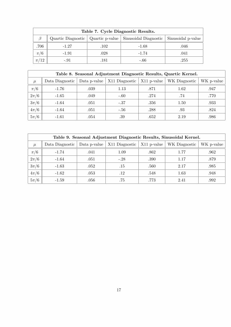
Table 7. Cycle Diagnostic Results.

β Quartic Diagnostic Quartic p-value Sinusoidal Diagnostic Sinusoidal p-value

.706 -1.27 .102 -1.68 .046

π/6 -1.91 .028 -1.74 .041

π/12 -.91 .181 -.66 .255

Table 8. Seasonal Adjustment Diagnostic Results, Quartic Kernel.

µ Data Diagnostic Data p-value X11 Diagnostic X11 p-value WK Diagnostic WK p-value

π/6 -1.76 .039 1.13 .871 1.62 .947

2π/6 -1.65 .049 -.60 .274 .74 .770

3π/6 -1.64 .051 -.37 .356 1.50 .933

4π/6 -1.64 .051 -.56 .288 .93 .824

5π/6 -1.61 .054 .39 .652 2.19 .986

Table 9. Seasonal Adjustment Diagnostic Results, Sinusoidal Kernel.

µ Data Diagnostic Data p-value X11 Diagnostic X11 p-value WK Diagnostic WK p-value

π/6 -1.74 .041 1.09 .862 1.77 .962

2π/6 -1.64 .051 -.28 .390 1.17 .879

3π/6 -1.63 .052 .15 .560 2.17 .985

4π/6 -1.62 .053 .12 .548 1.63 .948

5π/6 -1.59 .056 .75 .773 2.41 .992

17

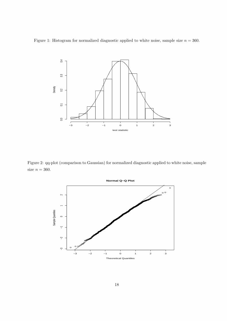
Figure 1: Histogram for normalized diagnostic applied to white noise, sample size n = 360.

test statistic

Dens

ity

−3 −2 −1 0 1 2 3

0.00.1

0.20.3

0.4

Figure 2: qq-plot (comparison to Gaussian) for normalized diagnostic applied to white noise, sample

size n = 360.

−3 −2 −1 0 1 2 3

−3−2

−10

12

Normal Q−Q Plot

Theoretical Quantiles

Samp

le Qu

antile

s

18

Figure 3: Logarithm of U.S. GDP, 1870− 1998.

Log Annual GDP

Year

1880 1900 1920 1940 1960 1980 2000

1213

1415

Figure 4: AR Spectrum of differenced logged U.S. GDP.

0.0 0.1 0.2 0.3 0.4 0.5

0.001

0.002

0.005

0.010

frequency

log sp

ectru

m

Log GDP Spectrum

19

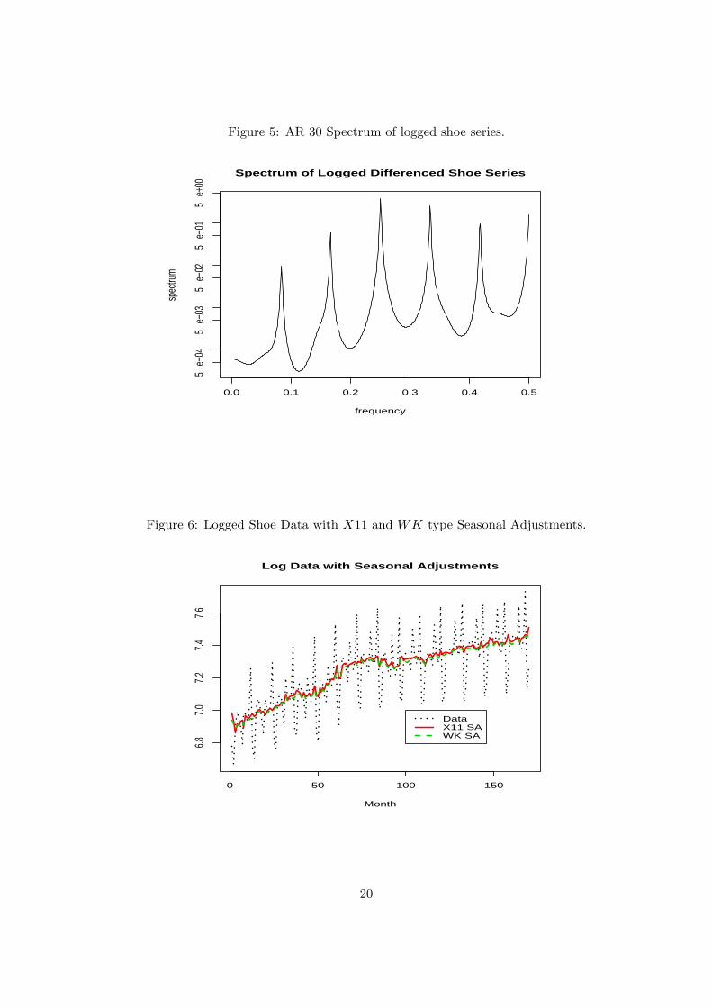
Figure 5: AR 30 Spectrum of logged shoe series.

0.0 0.1 0.2 0.3 0.4 0.5

5 e−

045

e−03

5 e−

025

e−01

5 e+

00

frequency

spec

trum

Spectrum of Logged Differenced Shoe Series

Figure 6: Logged Shoe Data with X11 and WK type Seasonal Adjustments.

Log Data with Seasonal Adjustments

Month

0 50 100 150

6.87.0

7.27.4

7.6

DataX11 SAWK SA

20

Figure 7: AR 30 Spectrum of differenced X11 Adjusted Shoe Data.

0.0 0.1 0.2 0.3 0.4 0.51 e−

045

e−04

2 e−

03

frequency

spec

trum

Spectrum of Differenced X−12 Adjustment

Figure 8: AR 30 Spectrum of differenced WK Adjusted Shoe Data.

0.0 0.1 0.2 0.3 0.4 0.5

5 e−

052

e−04

1 e−

03

frequency

spec

trum

Spectrum of Differenced WK Adjustment

21