Tuan V. Nguyen

Tuan V. Nguyen Garvan Institute of Medical Research

Sydney, Australia

Garvan Institute Biostatistical Workshop 16/7/2015 © Tuan V. Nguyen

Analysis of variance

• Between-group and within-group variation explained

• Model of ANOVA

• Post-hoc comparisons

• R implementation

Between-group variation andWithin-group variation

Sir Ronald A. Fisher, inventor of ANOVA

Ronald A. Fisher, geneticist, statistician, philosopher

"a genius who almost single-handedly created the foundations for modern statistical science"

"Fisher laid the foundations for most of experimental design, analysis of variance and much of statistical inference,"

Ronald Fisher (1890 – 1962)

The idea of ANOVA

• Analysis variable (Y) is continuous

• Comparison of multiple groups (k >2)

• Null hypothesis: all means are equal

Ho: µ1 = µ2 = …= µk

• Alternative hypothesis Ha: at least one pair is different

The concept of "variation"

• Given a series of n observed values Xi (X1, X2, X3, …) a deviate is defined as:

D = Xi – M

• Squared D:

D2 = (Xi - M)2

• Sum of squares (eg variation):

SS = (X1 - M)2 + (X2 - M)2 + (X3 - M)2 + … + (Xn - M)2

= ( )å=

-n

i i MX1

2

Between- and within-group variation

Key to understanding ANOVA:

• Between-group variation

• Within-group variation

"Between-group" variation

Group 1 Group 2 Group 3 Group k

X11 X21 X31 Xk1

X12 X22 X32 Xk2

X13 X23 X33 Xk3

X14 X24 X34 Xk4

X15 X25 X35 Xk5

X16 X26 X36 Xk6

M1 M2 M3 Mk

"Within-group" variation


X11 X21 X31 Xk1

X12 X22 X32 Xk2

X13 X23 X33 Xk3

X14 X24 X34 Xk4

X15 X25 X35 Xk5

X16 X26 X36 Xk6

M1 M2 M3 Mk

Logic ofANOVA


X11 X21 X31 Xk1

X12 X22 X32 Xk2

X13 X23 X33 Xk3

X14 X24 X34 Xk4

X15 X25 X35 Xk5

X16 X26 X36 Xk6

M1 M2 M3 Mk

• Compare between variation (B) with within group variation (W)

• If B > W, then that is a signal of difference between groups

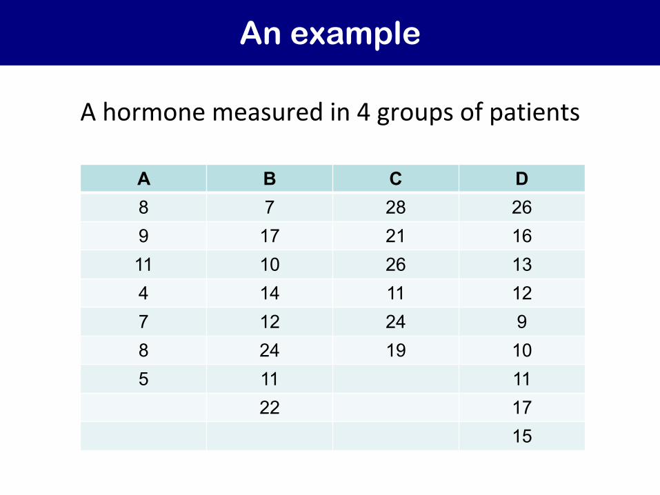
An example

A hormone measured in 4 groups of patients

A B C D 8 7 28 26 9 17 21 16 11 10 26 13 4 14 11 12 7 12 24 9 8 24 19 10 5 11 11

22 17 15

Between-group variation

A B C D 8 7 28 26 9 17 21 16 11 10 26 13 4 14 11 12 7 12 24 9 8 24 19 10 5 11 11

22 17 15

7.4 14.6 21.5 14.3Mean

Overall mean = 14.2

Between-group variation

A B C D

7.4 14.6 21.5 14.37 8 6 9

Mean

N

Overall mean = 14.2

Sum of squares of between-group differences:

SSB = 7*(7.4 – 14.2)2 + 8*(14.6 – 14.2)2 + 6*(21.5 – 14.2)2 + 9*(14.3 – 14.2)2 = 643.9

Within-group variation

A B C D 8 7 28 26 9 17 21 16 11 10 26 13 4 14 11 12 7 12 24 9 8 24 19 10 5 11 11

22 17 15

7.4 14.6 21.5 14.3Mean

Sum of within-group sum of squares:

SSWA = (8 – 7.4)2 + (9 – 7.4)2 + ... + (5 – 7.4)2 = 33.7


A B C D 8 7 28 26 9 17 21 16 11 10 26 13 4 14 11 12 7 12 24 9 8 24 19 10 5 11 11

22 17 15

7.4 14.6 21.5 14.3Mean

SSWA = (8 – 7.4)2 + (9 – 7.4)2 + ... + (5 – 7.4)2 = 33.7SSWB = 247.9SSWC = 185.5SSWD = 214.6


SSWA = (8 – 7.4)2 + (9 – 7.4)2 + ... + (5 – 7.4)2 = 33.7

SSWB = 247.9

SSWC = 185.5

SSWD = 214.6

SSW = 33.7 + 247.9 + 185.5 + 214.6 = 681.6

ANOVA table

Source Degrees of

freedom

Sum of squares

(SS)

Mean square (MS)

Between groups 643.9 Within group 681.6

Bảng phân tích phương sai

Source Degrees of freedom

Sum of squares

(SS)

Mean square (MS)

Between groups 3 643.9 214.6Within group 26 681.6 26.2Total 29 1325.5

F-test = 214.6 / 26.2 = 8.2

R codes

A = c(8, 9, 11, 4, 7, 8, 5)B = c(7, 17, 10, 14, 12, 24, 11, 22)C = c(28, 21, 26, 11, 24, 19)D = c(26, 16, 13, 12, 9, 10, 11, 17, 15)

x = c(A, B, C, D)group = c(rep("A", 7), rep("B", 8), rep("C", 6), rep("D", 9))

data = data.frame(x, group)data

av = aov(x ~ group)summary(av)

Result

> av=aov(x ~ group)> summary(av)

Df Sum Sq Mean Sq F value Pr(>F) group 3 642.3 214.09 8.197 0.000528 ***Residuals 26 679.1 26.12 ---Signif. codes: 0 ‘***’ 0.001 ‘**’ 0.01 ‘*’ 0.05 ‘.’ 0.1 ‘ ’ 1

There is a difference between groups

Analysis of variance: Summary

• ANOVA is used for testing the hypothesis that involves comparison of multiple groups

• R function for ANOVA: aov

analysis = aov(y ~ group)

Post hoc analyses

Multiple tests of hypothesis

• A study with m groups, the number of possible comparisons is:

( )21-mm

• Each pairwise comparison we have a 5% chance of resulting in a type I error (assuming a = 5%)

Comparison 1P=0.95

P=0.05

Accept H0

Reject H0

P(Accept,Accept) = 0.95*0.95

=0.9025

P(Accept,Reject) = 0.95*0.05

=0.0475

P(Reject,Accept) = 0.05*0.95

=0.0475

P(Reject,Reject) = .05*0.05

=0.0025

Accept H0

Reject H0

Accept H0

Reject H0

P=0.95

P=0.05

P=0.95

P=0.05

Comparison 2

When there are multiple tests

Inflation of type I error

• Type I error: Probability of significance (P < a) when there is in fact no difference

• Multiple tests of hypothesis à increase in type I error– For a single test, type I error = a

– For 6 tests, with a = 0.05, type I error = 1 – (1 – a)6 = 0.26

– For k tests, type I error = 1 – (1 – a)k

(This is also called experiment-wise error rate, family-wise type I error rate)

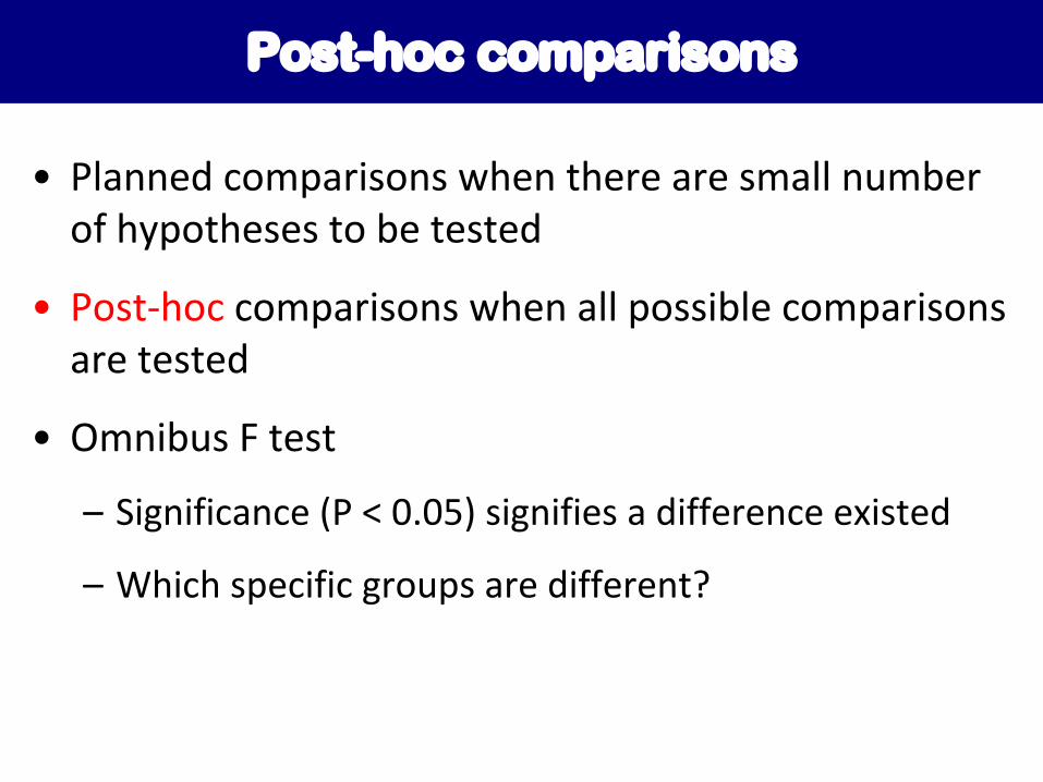
Post-hoc comparisons

• Planned comparisons when there are small number of hypotheses to be tested

• Post-hoc comparisons when all possible comparisons are tested

• Omnibus F test

– Significance (P < 0.05) signifies a difference existed

– Which specific groups are different?

Methods for post-hoc comparisons

• Classic methods

– Least significance difference (LSD): protected t test

– Bonferroni's adjustment

• Standard methods

– Tukey's Honestly Significant Difference

– Neuman-Keuls, Ryan, Scheffe, etc

• Newer / modern methods

– FDR

Least significance difference (LSD)

• Multiple t-test with no correction

t = X1 − X22MSerror

n

Carlo Emilio Bonferroni (1892 - 1960)

• Italian statistician, University of Florence

• Best known for "Bonferroni's inequality", and

• Bonferroni's correction in post-hoc analysis

Bonferroni's adjustment

• When there are c tests of hypothesis, the probability of finding a chance significance is 1 - (1 – α)c

• Correcting for multiple tests of hypothesis

• Use α* = α / c, where c is the number of tests

• If the observed P value < α*, then declare "significant"

Tukey’s HSD

• HSD = Honestly Significant Difference

/j kX X

QMSW n-

=

n is the average number of subjects per group

• If observed Q > theoretical Q (theoretical Tukey's Studentized critical value) then the difference is "statistically significant"

Tukey's studentized

• Studentized range statistic

• Difference between X1 and X2 is significant if:

• When n is not the same, then

N = 2ninj/(ni+nj)

, ,max mini i

k n kX XQ NWMSa-

-=

, ,i j

ij k n k

X X NQ Q

WMS a-

-= >

Newer method: False discovery rate (FDR)

• Advanced by Benjamini – Hochberg in a seminal paper (J Roy Statist Soc B 1995), almost 27,000 citations

• Question: How many false discoveries we have made?

FDR = # of falsely rejected null hypotheses total # of rejected null hypotheses

Benjamini & Hochberg's method

• Create a vector A of sorted p values

• Create a vector B by computing j(α/n) for j=1,2,...,n

• Substract vector A from vector B; call this vector C

• Find the largest index d, (from 1 to 10) for which the corresponding number in C is negative

• Reject all null hypotheses whose p values ≤ Pd

• The null hypothesis for all other tests are not rejected

FDR explained

• The FDR of a set of hypothesis tests is the expected percent of falsely rejected hypotheses.

• If FDR = 0.3, then we should expect 70% of them to be correct

Which method is appropriate?

The method that yields the

narrowest confidence interval

Adjustment for multiple comparisons

#Bonferroni

pairwise.t.test(x, group, p.adjust="bonferroni", pool.sd=T)

# Benjamin-Hochberg

pairwise.t.test(x, group, p.adjust="BH", pool.sd=T)

> pairwise.t.test(x, group, p.adjust="bonferroni", pool.sd=T)

Pairwise comparisons using t tests with pooled SD

data: x and group

A B C B 0.06876 - -C 0.00023 0.11673 -D 0.07547 1.00000 0.07911

> pairwise.t.test(x, group, p.adjust="BH", pool.sd=T)

Pairwise comparisons using t tests with pooled SD

data: x and group

A B C B 0.01978 - -C 0.00023 0.02335 -D 0.01978 0.90741 0.01978

P value adjustment method: BH

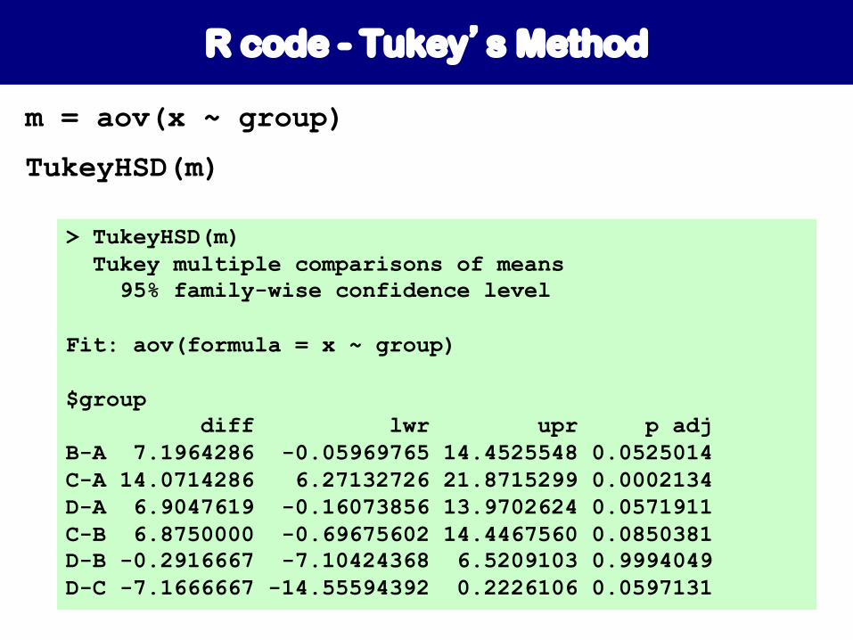
R code - Tukey’s Method

m = aov(x ~ group)

TukeyHSD(m)

> TukeyHSD(m)Tukey multiple comparisons of means95% family-wise confidence level

Fit: aov(formula = x ~ group)

$groupdiff lwr upr p adj

B-A 7.1964286 -0.05969765 14.4525548 0.0525014C-A 14.0714286 6.27132726 21.8715299 0.0002134D-A 6.9047619 -0.16073856 13.9702624 0.0571911C-B 6.8750000 -0.69675602 14.4467560 0.0850381D-B -0.2916667 -7.10424368 6.5209103 0.9994049D-C -7.1666667 -14.55594392 0.2226106 0.0597131

plot(TukeyHSD(m), ordered=T)

-10 0 10 20

D-C

D-B

C-B

D-A

C-A

B-A

95% family-wise confidence level

Differences in mean levels of group

ANOVA: summary

• ANOVA– An extension of 2-sample t-test to multiple groups

– Comparing between-group variation to within-group variation

• Many Post-hoc comparisons

– Help control type I error

– Beware of the alpha level and power issues

Tuan V. Nguyen

Documents