Welcome message from author
This document is posted to help you gain knowledge. Please leave a comment to let me know what you think about it! Share it to your friends and learn new things together.
Transcript


This page intentionally left blank

How to Price
A Guide to Pricing Techniques and Yield Management
Over the past four decades, business and academic economists, operations researchers,
marketing scientists, and consulting firms have increased their interest in and research on
pricing and revenue management. This book attempts to introduce the reader to a wide
variety of research results on pricing techniques in a unified, systematic way at varying levels
of difficulty. The book contains a large number of exercises and solutions and therefore can
serve as a main or supplementary course textbook, as well as a reference guide for pricing
consultants, managers, industrial engineers, and writers of pricing software applications.
Despite a moderate technical orientation, the book is accessible to readers with a limited
knowledge in these fields as well as to readers who have had more training in economics.
Most pricing models are first demonstrated by numerical and calculus-free examples and
then extended for more technically oriented readers.
Oz Shy is a Research Professor at WZB – Social Science Research Center in Berlin, Germany,
and a Professor of Economics at the University of Haifa, Israel. He received a BA degree
from the Hebrew University of Jerusalem and a PhD from the University of Minnesota. His
previous books are Industrial Organization: Theory and Applications (1996) and The Economics
of Network Industries (Cambridge University Press, 2001). Professor Shy has published more
than 40 journal and book articles in the areas of industrial organization, network economics,
and international trade, and he serves on the editorial boards of International Journal of
Industrial Organization, Journal of Economic Behavior & Organization, and Review of Network
Economics. He has taught at the State University of New York, Tel Aviv University, University
of Michigan, Stockholm School of Economics, and Swedish School of Economics at Helsinki.


How to Price
A Guide to Pricing Techniques and Yield Management
Oz ShyWZB – Social Science Research Center, Berlin, Germany
and
University of Haifa, Israel
CAMBRIDGE UNIVERSITY PRESS
Cambridge, New York, Melbourne, Madrid, Cape Town, Singapore, São Paulo
Cambridge University PressThe Edinburgh Building, Cambridge CB2 8RU, UK
First published in print format
ISBN-13 978-0-521-88759-5
ISBN-13 978-0-511-39467-6
© Oz Shy 2008
2008
Information on this title: www.cambridge.org/9780521887595
This publication is in copyright. Subject to statutory exception and to the provision of relevant collective licensing agreements, no reproduction of any part may take place without the written permission of Cambridge University Press.
Cambridge University Press has no responsibility for the persistence or accuracy of urls for external or third-party internet websites referred to in this publication, and does not guarantee that any content on such websites is, or will remain, accurate or appropriate.
Published in the United States of America by Cambridge University Press, New York
www.cambridge.org
eBook (NetLibrary)
hardback

For Sarah, Daniel, and Tianlai

Contents
Preface xi
1 Introduction to Pricing Techniques 11.1 Services, Booking Systems, and Consumer Value 2
1.2 Overview of Pricing Techniques 5
1.3 Revenue Management and Profit Maximization 9
1.4 The Role Played by Capacity 10
1.5 YM, Consumer Welfare, and Antitrust 12
1.6 Pricing Techniques and the Use of Computers 13
1.7 The Literature and Presentation Methods 14
1.8 Notation and Symbols 14
2 Demand and Cost 192.1 Demand Theory and Interpretations 20
2.2 Discrete Demand Functions 24
2.3 Linear Demand Functions 26
2.4 Constant-elasticity Demand Functions 30
2.5 Aggregating Demand Functions 34
2.6 Demand and Network Effects 39
2.7 Demand for Substitutes and Complements 42
2.8 Consumer Surplus 45
2.9 Cost of Production 52
2.10 Exercises 56
3 Basic Pricing Techniques 593.1 Single-market Pricing 60
3.2 Multiple Markets without Price Discrimination 67
3.3 Multiple Markets with Price Discrimination 79
3.4 Pricing under Competition 89
3.5 Commonly Practiced Pricing Methods 99
3.6 Regulated Public Utility 104
3.7 Exercises 110
viii Contents
4 Bundling and Tying 1154.1 Bundling 117
4.2 Tying 131
4.3 Exercises 145
5 Multipart Tariff 1515.1 Two-part Tariff with One Type of Consumer 152
5.2 Two-part Tariff with Multiple Consumer Types 159
5.3 Menu of Two-part Tariffs 165
5.4 Multipart Tariff 171
5.5 Regulated Public Utility 176
5.6 Exercises 178
6 Peak-load Pricing 1816.1 Seasons, Cycles, and Service-cost Definitions 183
6.2 Two Seasons: Fixed-peak Case 185
6.3 Two Seasons: Shifting-peak Case 190
6.4 General Computer Algorithm for Two Seasons 194
6.5 Multi-season Pricing 194
6.6 Season-interdependent Demand Functions 201
6.7 Regulated Public Utility 205
6.8 Demand, Cost, and the Lengths of Seasons 214
6.9 Exercises 223
7 Advance Booking 2277.1 Two Booking Periods with Two Service Classes 232
7.2 Multiple Periods with Two Service Classes 238
7.3 Multiple Booking Periods and Service Classes 245
7.4 Dynamic Booking with Marginal Operating Cost 248
7.5 Network-based Dynamic Advance Booking 250
7.6 Fixed Class Allocations 254
7.7 Nested Class Allocations 258
7.8 Exercises 262
8 Refund Strategies 2658.1 Basic Definitions 267
8.2 Consumers, Preferences, and Seller’s Profit 270
8.3 Refund Policy under an Exogenously Given Price 274
8.4 Simultaneous Price and Refund Policy Decisions 280
8.5 Multiple Price and Refund Packages 288
8.6 Refund Policy under Moral Hazard 290
8.7 Integrating Refunds within Advance Booking 293
8.8 Exercises 294

Contents ix
9 Overbooking 2979.1 Basic Definitions 299
9.2 Profit-maximizing Overbooking 305
9.3 Overbooking of Groups 313
9.4 Exercises 322
10 Quality, Loyalty, Auctions, and Advertising 32510.1 Quality Differentiation and Classes 326
10.2 Damaged Goods 332
10.3 More on Pricing under Competition 335
10.4 Auctions 343
10.5 Advertising Expenditure 352
10.6 Exercises 355
11 Tariff-choice Biases and Warranties 35911.1 Flat-rate Biases 360
11.2 Choice in Context and Extremeness Aversion 362
11.3 Other Consumer Choice Biases 366
11.4 Warranties 369
11.5 Exercises 375
12 Instructor and Solution Manual 37712.1 To the Reader 377
12.2 Manual for Chapter 2: Demand and Cost 378
12.3 Manual for Chapter 3: Basic Pricing Techniques 382
12.4 Manual for Chapter 4: Bundling and Tying 387
12.5 Manual for Chapter 5: Multipart Tariff 391
12.6 Manual for Chapter 6: Peak-load Pricing 395
12.7 Manual for Chapter 7: Advance Booking 402
12.8 Manual for Chapter 8: Refund Strategies 406
12.9 Manual for Chapter 9: Overbooking 411
12.10 Manual for Chapter 10: Quality, Loyalty, Auctions, and
Advertising 414
12.11 Manual for Chapter 11: Tariff-choice Biases and Warranties 417
References 421
Index 431


Preface
What This Book Will NOT Teach You
The key to successful profit-maximizing pricing is knowing your potential cus-tomers. If a firm does not manage to learn the characteristics of all its potential
customer types, such as consumers’ willingness to pay, the firm will not be able to
properly price its products and services.
This book will not teach you how to identify the characteristics of your con-
sumers. Although several econometric techniques for identifying these characteris-
tics are described in Chapter 2, a comprehensive analysis of this subject is beyond
the scope of this book. The two main reasons for not attempting to include these
techniques in this book are (a) consumers’ preferences in general, and willingness
to pay in particular, vary all the time when new competing products, services, and
brands are introduced to the market, which means that (b) the most efficient way of
learning about customers is by trial and error, or simply experimenting with dif-
ferent tariffs while recording how consumers respond. That is, as this book shows,
successful pricing techniques should not only be profitable, they should also induce
consumers to reveal their characteristics.
What This Book Attempts to Teach You
Revenue and profit are affected by a wide variety of observable and unobserv-
able parameters. Therefore, even if various pricing techniques are well chosen and
properly used, there is still no guarantee that the firm will be profitable. However,
despite the high degree of uncertainty, if one takes the approach that pricing with
some reasoning cannot be inferior (profitwise) to implementing arbitrary pricing
strategies, then it is hoped this book will provide you with the right intuition and
with a wide variety of tools under which sellers can enhance their profits. During
the past 40 years, business and academic economists, operations researchers, mar-
keting scientists, and consulting firms have increased their interest in and research
on pricing and revenue management. This book attempts to introduce the reader
to a wide variety of their research results in a unified systemic way, but at vary-
ing levels of difficulty. Traditionally, the different disciplines manifested different
views on pricing techniques; however, recently the attitudes toward pricing in these

xii Preface
disciplines have exhibited a sharp convergence that recognizes price discrimination
and market segmentation as an important part of the design of profitable pricing
techniques. It is hoped that the present book contributes to this convergence pro-
cess.
Motivation for Writing This Book
Yield and revenue management (or profit management, as it should be called) is
commonly taught in business schools, where very often teachers simply combine it
with a marketing course. Revenue management is also taught in special courses and
seminars for employees of the airline and hotel industries. Most of these special
courses tend to be nontechnical. All this means that the analytical work on yield
management, which was written mainly by scientists in the field of operations re-
search, cannot be diffused to the general audience. Such a diffusion is not always
needed, however, given that large companies tend to rely on software packages and
automated reservation systems.
On the other side of the campus, the economics profession has managed over
the years to develop a large number of theories on profitable pricing techniques.
Most of these techniques are based on price discrimination. Other theories come
from extensive research conducted by economists during the 1970s and 1980s on
optimal regulation and deregulation of public utilities. Often, the economics ap-
proach goes somewhat further than the operations research approach by consider-
ing the strategic response of rival firms competing in the same market.
The purpose of this book is to combine the relevant theories from economics
(mainly from microeconomics, industrial organization, and regulation) with some
operations research, and to make it accessible to students and practitioners who
have limited knowledge in these fields. On the other hand, readers who have had
more training in economics will easily find more advanced material. Knowledge of
calculus is not needed for the major part of this book, because calculus techniques
are not very useful for handling discrete data, which a computer can manipulate.
However, more mathematically trained readers should be able to find various topics
and extensions that are based on calculus. To summarize, this book attempts to
introduce the formal analysis of revenue management and pricing techniques by
bridging the knowledge gained from economic theory and operations research. This
book is also designed as a reference guide for pricing consultants and managers as
well as computer programmers who are equipped with the appropriate technical
knowledge.

Preface xiii
Computer Applications
Professional price practitioners may want to simulate the studied pricing techniques
on a computer to ultimately bring these techniques to practical use. For this reason,
I have attempted to sketch some algorithms according to which programmers can
write simple macros. These macros can be easily written using popular spread-
sheet software and thus do not always require sophisticated programming. Of
course, some readers may feel more comfortable writing in formal programming
languages. The reader is invited to visit the Web site www.how-to-price.comto observe how these short macros can be implemented on the Web using the
JavaScript language. Clearly, limited space does not allow me to write complete
algorithms. But I hope that the logic behind the suggested algorithms would benefit
the potential programmer by serving as a benchmark for more sophisticated pricing
software. For convenience, the algorithms in this book are written to resemble algo-
rithms in Pascal (a computer programming language designed in 1970 for teaching
students structured programming).
To the Instructor
The instructor will find sufficient material to fill at least a one-semester course,
if not an entire year. This book uses lots of calculus-free models, so it can be
used without calculus if needed. An instructor’s manual is provided in Chapter 12,
where I also provide abbreviated solutions for all exercises. I urge the instructor
to read this manual before writing the course syllabus because for each chapter, I
provide some suggestions regarding which topics should suit students with different
backgrounds.
Basically, the book can be divided into three parts. Although topics from all
chapters are interrelated, Chapters 2 through 5 may be classified as pricing tech-
niques (mostly for static and stationary markets). Chapters 6 through 9 roughly
fall under the category of yield and revenue management as they analyze dynamic
markets under capacity constraints. Chapters 10 and 11 offer a variety of topics
related to both pricing and revenue management.
Each chapter ends with several exercises. These exercises attempt to moti-
vate students to understand and memorize the basic definitions associated with the
various theories developed in that chapter. The solution to all these exercises are
provided in Chapter 12. Providing all the solutions to students has its pros and
cons. However, I have found that students who go over these solutions perform
much better on the exams than do students who are not exposed to the solutions.
As a result, instead of placing the solution manual on the Internet (as I have done
for my other books), I have integrated the solutions into the book itself.

xiv Preface
This book is clearly on the technical side. However, most topics in this book
are covered at multiple levels of difficulty. Hence, numerical examples should
appeal to the less technical reader, whereas the general formulations and computer
algorithms should appeal to more technical readers and researchers. Topics from
this book can be arranged as a one-semester course for advanced undergraduate
and graduate students in economics, as well as for those in some advanced MBA
programs that go beyond the purely descriptive case-based method. Students of
industrial engineering should also be able to grasp most of the material.
Errors, Typos, and Errata Files
My experience with my first two books (Shy 1996, 2001) has been that it is nearly
impossible to publish a completely error-free book. Writing a book very much
resembles writing a large piece of software because literally all software pack-
ages contain some bugs that the author could not predict. In addition, 80% of the
time is devoted to debugging the software after the basic code has been written. I
will therefore make an effort to publish all errors known to me on my Web site:
www.ozshy.com.
Typesetting and Acknowledgments
This book was typeset by the author using the LATEX 2ε document preparation soft-
ware developed by Leslie Lamport (a special version of Donald Knuth’s TEX pro-
gram) and modified by the LATEX3 Project Team. For most parts, I used MikTEX,
developed by Christian Schenk, as the main compiler.
Staffan Ringbom, Swedish School of Economics at Helsinki and HECER, has
offered many suggestions, ideas, and comments that greatly improved the exposi-
tion and the content of this book. In addition, Staffan was the first to teach this book
in a university environment and to collect some comments directly from students.
I also would like to thank the Social Science Research Center Berlin (WZB) for
providing me with the best possible research environment, which enabled me to
complete this book in only two years.
During the preparation of the manuscript, I was very fortunate to work with
Scott Parris of Cambridge University Press, to whom I owe many thanks for man-
aging the project in the most efficient way. Scott has been fond of this project for
several years, and his interest in this topic encouraged me to go ahead and write this
book. Finally, I thank Barbara Walthall of Aptara, Inc. and the entire Cambridge
University Press team for the fast production of this book.
Berlin, Germany (May 2007)
www.ozshy.com
Chapter 1
Introduction to Pricing Techniques
1.1 Services, Booking Systems, and Consumer Value 2
1.1.1 Service definitions
1.1.2 Dynamic reservation systems
1.1.3 Consumer value
1.2 Overview of Pricing Techniques 5
1.2.1 Why is price discrimination needed?
1.2.2 Classifications of market segmentation
1.2.3 Classifications of price discrimination
1.3 Revenue Management and Profit Maximization 9
1.4 The Role Played by Capacity 10
1.4.1 Price-based YM under capacity constraints
1.4.2 Quantity-based YM versus price-based YM
1.5 YM, Consumer Welfare, and Antitrust 12
1.6 Pricing Techniques and the Use of Computers 13
1.7 The Literature and Presentation Methods 14
1.8 Notation and Symbols 14
This book focuses on pricing techniques that enable firms to enhance their profits.
This book, however, cannot provide a complete recipe for success in marketing a
certain product as this type of recipe, if it existed, would depend on a very large
number of factors that cannot be analyzed in a single book. However, what this
book does offer is a wide variety of pricing methods by which firms can enhance
their revenue and profit. Such pricing strategies constitute part of the field called
yield management. As explained and discussed in Section 1.3, throughout this book
we will be using the term yield management (YM) to mean profit management
and profit maximization, as opposed to the more commonly used term revenuemanagement (RM).
2 Introduction to Pricing Techniques
1.1 Services, Booking Systems, and Consumer Value
Before we discuss pricing techniques, we wish to characterize the “output” that
firms would like to sell. Therefore, Subsection 1.1.1 defines and characterizes
the type of services and goods for which YM turns out to be most useful as a
profit-enhancing set of tools. Clearly, this book emphasizes services that constitute
around 70% of the gross domestic product of a modern economy. Subsection 1.1.2
identifies dynamic industry characteristics that make YM pricing techniques highly
profitable. These characteristics highlight the role of the timing under which the po-
tential consumers approach the sellers for the purpose of booking and purchasing
the services sellers provide. Subsection 1.1.3 discusses the difficulty in determining
consumer value and willingness to pay for services and products.
1.1.1 Service definitions
YM pricing techniques will not enhance the profit of every seller of goods and
services. YM pricing techniques are particularly profitable for selling services, for
the following reasons:
• Nonstorability: Services are time dependent and are therefore nonstorable. This
feature is essential as otherwise service providers could transfer unused capacity
from one service date to another. For example, airline companies cannot transfer
unsold seats from one aircraft to another. Hotel managers cannot “save” vacant
rooms for future sales.
• Advance purchase/booking: Time of purchase need not be the same as the ser-
vice delivery time. In this book we demonstrate how reservation systems can be
designed to enhance profits from the utilization of a given capacity level. For
example, we show how airline companies can exploit consumer heterogeneity
with respect to their ability to commit to buying services.
• No-shows and cancellations: Consumers who book in advance may not show
up and may even cancel their reservation. Service providers should be able to
segment the market according to how much refund (if any) is given upon no-
shows.
• Service classes: The service can be provided in different quality classes. Market
segmentation is profitable whenever the difference in price between, say, first
and second class exceeds the difference in marginal costs.
The first item on the list is essential for the practice of YM to be profitable. The
second item is not essential but definitely helps to generate extra revenue from seg-
menting the market according to the time reservations are made. The third item on

1.1 Services, Booking Systems, and Consumer Value 3
the list also applies to physical products (as opposed to services) because sellers of-
ten practice refund policies for goods in the form of monetary refunds and product
replacements.
1.1.2 Dynamic reservation systems
As it turns out, the procedure under which consumers buy or reserve a service
can be viewed as part of the service itself. Moreover, another characteristic of the
type of many of the services analyzed in this book is that consumers make their
reservations at different time periods. More precisely, some consumers reserve the
service long before the service is scheduled to be delivered. Others make last-
minute reservations.
In the absence of full refunds on purchased services, an early reservation re-
flects a commitment on the part of the consumer. Service providers can exploit
different levels of willingness to commit by offering discounts to those consumers
who are willing to make an early commitment, and charge higher prices for a last-
minute booking.
The airline industry was perhaps the first industry to fully computerize reserva-
tion systems. It was also the first to systematically discriminate in price according
to when bookings are made. During the late 1980s, these computerized reservation
systems (CRS) were perfected and became fully dynamic so that capacity alloca-
tions could be revised according to which types of reservations were already made
in addition to which reservation types would be expected to emerge before the ser-
vice delivery time.
This discussion and the analysis provided in this book should help us under-
stand the following observed phenomena, for example:
(a) Why travelers sitting in the same economy class on the same flight pay different
airfares. Why people who stay at identical hotel room sizes end up paying
different prices.
(b) Why capacity underutilization is often observed, such as empty seats on an
aircraft and vacant hotel rooms.
Roughly speaking, the answer to (a) is that profit is enhanced when passengers
and consumers pay near their maximum willingness to pay. Therefore, as long as
consumers are heterogeneous with respect to their willingness to pay, proper use
of YM always results in having people paying different prices for what appears to
be an identical service. This is implemented via market segmentation, discussed in
Subsection 1.2.2.
The answer to (b) is that because service providers seek to maximize profit, it
may become profitable not to sell the entire capacity but to leave some capacity in
case consumers with high willingness to pay show up at the last minute. If they
4 Introduction to Pricing Techniques
don’t, then sellers are left with unused capacity. However, the reader may be won-
dering at this point whether profit is indeed maximized and may be asking why ser-
vice providers do not at the last minute sell unused capacity at low prices, thereby
avoiding empty seats and vacant rooms. The answer is simple. If consumers ob-
serve that a certain service provider sells discounted tickets at the last minute, they
may be deterred from making early reservations. Thus, service providers may suf-
fer from a bad reputation if they often practice last-minute discounts. This is known
as the sellers’ commitment problem. That is, in the short run, service providers may
find it profitable to sell last-minute unbooked capacity at a lower price just to fill
up the entire capacity. However, long-run considerations, such as reputation effect,
prevent such practices.
1.1.3 Consumer value
The main point that this book attempts to stress is that sellers earn much higher
profit if they set prices according to consumer value as opposed to basing all pricing
decisions on unit cost only. It is not rare to hear managers state that their profits
are generated by charging consumers a certain fixed markup above unit cost. In
most cases, such cost-based pricing techniques fail to extract a large part of what
consumers are actually willing to pay.
In view of this discussion, the “conflict” between buyers and sellers, particu-
larly if the two parties allow bargaining to take place, is manifested in the following
two rules:
Rule for sellers: Make an effort to set the price according to buyers’ value and not
according to cost.
Rule for buyers: Bargain, if you can, for prices closer to marginal cost.
Note that the rule for sellers becomes essential for services produced at near-zero
marginal costs, such as those provided on the Internet.
With a few exceptions, throughout this book it is assumed that sellers know the
consumers’ value and willingness to pay for the services and products they sell. The
firms may not know the exact valuation of a specific consumer, but it is assumed
that they know the distribution of the willingness to pay among different consumer
groups. Clearly, firms should exert a lot of effort to unveil these valuations. For
demand functions, the next chapter shows how this can be done by running re-
gressions on data on past sales collected from the market. However, because these
data are not always available, firms may resort to market surveys. Market surveys
are less reliable because consumers don’t always understand the question they are
asked, and even if they do, they may understate their willingness to pay.
In cases in which the seller faces competition from other firms selling similar
products and services, consumers may base their willingness to pay on the prices
charged by the competing firms, that is, by placing a reference value for the product
1.2 Overview of Pricing Techniques 5
or service. In this situation, the seller must carefully study and compare the features
of products and services offered by his or her competitors with the features of
the product or service he or she offers. In fact, as often argued in this book, the
seller should attempt to differentiate his or her brand from competing brands, by
adding more features, including his or her services. Clearly, a lack of features
relative to competing brands would necessitate a price reduction. After translating
the observed differences between brands into their monetary equivalent, a seller
should determine consumer value by
Value of the brand = Reference value
+ “Positive” differentiation values− “Negative” differentiation values.
The above formula relies on the assumption that all consumers agree on the pluses
and minuses of each brand, which need not always be the case – for example, in
markets where the brands are horizontally differentiated (as opposed to vertically
differentiated).
Finally, there are other factors that affect consumers’ willingness to pay for a
certain brand, including:
Switching costs: If the seller is an established firm with a large number of returning
customers, the seller can add to the price the cost consumers would pay to
switch to a competing brand. If the seller is a new entrant, the seller may want
to reduce the price to subsidize consumer switching costs; see the analysis in
Section 3.4.
Essential input: Sellers can augment the price in cases in which the product/service
serves as an essential input to goods and services produced by buyers. Some
economists refer to this type of action as the “holdup problem.”
Location costs: When reference prices are used, the cost of shipping or the location
of the service should be reflected in the price, or shared by the parties.
1.2 Overview of Pricing Techniques
YM pricing techniques are not cost based. On the contrary, the key to successful
YM is to make different consumers pay different prices for what seem to be iden-
tical services. The key to profit-enhancing pricing plans is the ability to engage
in price discrimination via what economists call market segmentation. Price dis-crimination prevails if different (groups of) consumers pay different prices for what
appears to be the same or a similar service or good. Market segmentation prevails
whenever firms manage to divide the market into subgroups of consumers in which
consumers belonging to different groups end up paying different prices.
6 Introduction to Pricing Techniques
1.2.1 Why is price discrimination needed?
An inexperienced reader may wonder why price discrimination is so important and
ask why a strategy whereby all consumers are charged the same price is generally
not profit maximizing? The answer to this question is that the practice of price dis-
crimination enables service providers to enlarge their customer base and to create
new markets. Consider the following example taken from a market for classical
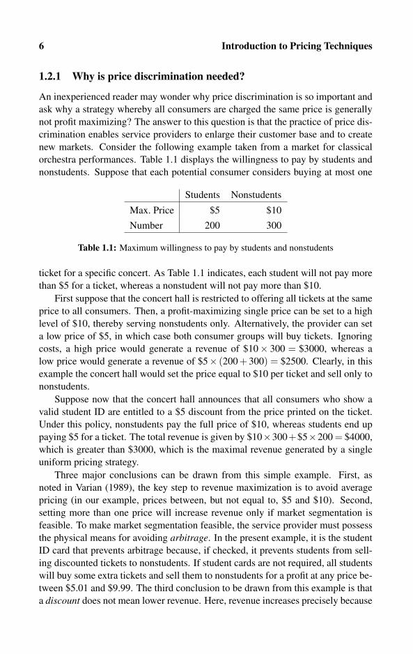
orchestra performances. Table 1.1 displays the willingness to pay by students and
nonstudents. Suppose that each potential consumer considers buying at most one
Students Nonstudents
Max. Price $5 $10
Number 200 300
Table 1.1: Maximum willingness to pay by students and nonstudents
ticket for a specific concert. As Table 1.1 indicates, each student will not pay more
than $5 for a ticket, whereas a nonstudent will not pay more than $10.
First suppose that the concert hall is restricted to offering all tickets at the same
price to all consumers. Then, a profit-maximizing single price can be set to a high
level of $10, thereby serving nonstudents only. Alternatively, the provider can set
a low price of $5, in which case both consumer groups will buy tickets. Ignoring
costs, a high price would generate a revenue of $10× 300 = $3000, whereas a
low price would generate a revenue of $5× (200 + 300) = $2500. Clearly, in this
example the concert hall would set the price equal to $10 per ticket and sell only to
nonstudents.
Suppose now that the concert hall announces that all consumers who show a
valid student ID are entitled to a $5 discount from the price printed on the ticket.
Under this policy, nonstudents pay the full price of $10, whereas students end up
paying $5 for a ticket. The total revenue is given by $10×300+$5×200 = $4000,
which is greater than $3000, which is the maximal revenue generated by a single
uniform pricing strategy.
Three major conclusions can be drawn from this simple example. First, as
noted in Varian (1989), the key step to revenue maximization is to avoid average
pricing (in our example, prices between, but not equal to, $5 and $10). Second,
setting more than one price will increase revenue only if market segmentation is
feasible. To make market segmentation feasible, the service provider must possess
the physical means for avoiding arbitrage. In the present example, it is the student
ID card that prevents arbitrage because, if checked, it prevents students from sell-
ing discounted tickets to nonstudents. If student cards are not required, all students
will buy some extra tickets and sell them to nonstudents for a profit at any price be-
tween $5.01 and $9.99. The third conclusion to be drawn from this example is that
a discount does not mean lower revenue. Here, revenue increases precisely because
1.2 Overview of Pricing Techniques 7
student cards make it possible to lower the price for low-valuation consumers. In
fact, later on we will analyze a similar strategy in which damaging a good (artifi-
cially lowering the quality of the service) can also enhance sales revenue.
1.2.2 Classifications of market segmentation
The above discussion was intended to convince the reader that market segmentation
is necessary for the success of any price discrimination strategy. Broadly speaking,
a market can be segmented along the following dimensions:
• Consumer identifiable characteristics: Charging different prices according to
age group, profession, affiliation, location, type of delivery, and means of pay-
ment.
• Quality: Selling high-quality versions of the product/service to high-income buy-
ers, and low-quality versions to low-income buyers. Segmentation of this type
is possible only if the desire for higher quality increases with income. Note
that firms often reduce quality (damaging the good/service) to keep differential
pricing.
• Bundling and tying: Bundling refers to volume discounts. Segmentation of this
type is possible only if consumers have different demand elasticity with respect
to the quantity they purchase. Tying refers to selling packages of different goods
at a single price. This market segmentation is profitable when consumer prefer-
ences for the different goods are negatively correlated.
• Delivery time and delay: The seller segments the market according to con-
sumers’ willingness to pay for how fast the product or service is provided or
delivered. This segmentation is feasible provided that those consumers who ur-
gently need the product or service are willing to pay a higher amount than those
who don’t mind waiting.
• Components: Sellers can segment the market by mixing different components
and providing a different number of components comprising the system to be
used by the buyer. This strategy is commonly observed in the software industry,
where a piece of software is sold in standard, pro, and professional versions.
• Advance booking and refunds: Sellers can segment the market based on con-
sumers’ willingness to commit to showing up at the time the service is scheduled
to be delivered. Market segmentation is achieved by charging lower prices either
to those who reserve in advance or to those who seek less refund on a no-show.
Conversely, those who seek to obtain a full refund on a no-show are charged a
higher price.
As this book will make clear, these classifications are not mutually exclusive. To
the contrary, many types of the above-listed segmentations are often combined into
8 Introduction to Pricing Techniques
a single pricing strategy. For example, book publishers tend to sell books with a
hard cover during the first year of publication. Then, the same book is printed with
a soft cover and sold at a lower price. Thus, consumers’ willingness to pay for the
first printing (fast delivery) seems to be correlated with the quality of the binding.
1.2.3 Classifications of price discrimination
Traditionally, academic economists (see, for example, Varian 1989) classify price
discrimination according to first, second, and third degrees as follows:
• First degree: Consumers may be charged different prices so that the price of each
unit they buy equals each consumer’s maximum willingness to pay.
• Second degree: Each consumer faces the same price schedule, but the sched-
ule involves different prices for different amounts of the good purchased. This
practice is sometimes referred to as bundling (quantity discounts).
• Third degree: The seller segments the market into different consumer groups
(with identifiable characteristics) that are charged different per-unit prices. This
practice is referred to as market segmentation.
In this book, we will not be making much use of these classifications because the
goal of this book is to characterize the proper pricing strategy to be able to seg-
ment the market, rather than just targeting a specific type of price discrimination
taken from the above list. That is, from a practical point of view, the firm should
be attempting to ensure that the chosen pricing techniques will indeed lead to the
desired market segmentation, and that the resulting segmentation is the most prof-
itable segmentation among all the feasible market segmentations. Moreover, the
problem with the above classifications (according to first, second, and third de-
grees) is that these three classifications are not mutually exclusive. For example,
second- and third-degree price discrimination can be implemented by, say, offer-
ing students different bundles from those offered to customers who cannot present
student identification cards. For this reason, we deviate from the traditional classi-
fications and follow the entry on price discrimination in Wikipedia, which suggests
the following classifications based on a seller’s ability to segment a market:
• Complete discrimination: Basically, the same as the first-degree price discrim-
ination described above. Each consumer purchases where the marginal benefit
equals the consumer-specific price.
• Direct segmentation: The seller segments the market into different consumer
groups (with identifiable characteristics).
• Indirect segmentation: The seller offers variations of the product based on qual-
ity, quantity, delivery time, bundled service, and so on. The proper use of this

1.3 Revenue Management and Profit Maximization 9
technique leads to self-selection of consumers according to their nonidentifiable
characteristics.
The reader should note that there is a fundamental difference between direct and
indirect segmentation. Direct segmentation is clearly more profitable but requires
the ability and knowledge to group consumers according to age, gender, geographic
location, profession, prior consumption record, and so on. However, if this knowl-
edge is not available (or illegal under nondiscrimination laws), sellers must resort
to the less profitable indirect segmentation, which relies on selecting product and
service variations instead of directly selecting different consumer groups. Finally,
complete segmentation is clearly the most profitable; however, it is unlikely to be-
come feasible (and more likely to be illegal) as it requires the seller to obtain full
characterization of each consumer separately.
1.3 Revenue Management and Profit Maximization
Students of economics generally fail to understand why academic and nonacademic
business people use the terms yield and revenue management as the goal of their
pricing strategy. This is because economics students are always taught that firms
should attempt to maximize profit and that revenue maximization does not imply
profit maximization in the presence of strictly positive marginal costs.
However, as it turns out very often, profit-maximizing pricing strategies are
sometimes better understood in the context of revenue maximization rather than
by attempting to maximize profits even when all production costs are taken into ac-
count. In addition, with the ongoing information revolution and the fast penetration
of the Internet as the main source of information, yield and revenue management
can in many cases lead to profit-maximizing prices, mainly because most costs of
producing information are sunk whereas the cost of duplicating information ser-
vices could be negligible. But even if we ignore information products, there are
some industries that operate under significant capacity constraints, such as the air-
line and hotel industries. In these industries, most costs are sunk and indeed the
marginal costs can be ignored as long as the firms operate below their full capacity.
In view of this discussion, this book uses the term yield management to mean
the utilization of profit-maximizing pricing techniques. Therefore, we will gen-
erally avoid mentioning the commonly used term revenue management, although
recently it seems that the use of RM is gradually replacing the use of YM. Histor-
ically, YM was associated with early problems that treated price and capacity as
fixed and maximized “yield” or utilization of capital. This book, however, inter-
prets the term yield as profit.
To demonstrate why profit maximization differs from revenue maximization,
Table 1.2 displays the willingness to pay for a meal by three consumer groups:
students, civil servants, and members of parliament. When marginal cost is zero,

10 Introduction to Pricing Techniques
Students Civil Servants Parliament Members
Maximal Price: $5 $8 $10
# Consumers: 200 100 100
Marginal Cost Profit Levels
$0 2000 1600 1000
$4 400 800 600
$7 −800 200 300
Table 1.2: The effect of marginal cost on the choice of profit-maximizing price. Note:
Boldface figures are profit levels under the profit-maximizing price.
profit equals revenue. Under zero marginal cost, profit/revenue is $5(200 + 100 +100) = $2000 when the price is lowered to $5. Raising the price to $8 and $10
lowers the profit/revenue levels. Now, if the marginal cost equals 4, profit does not
equal revenue. Clearly, the revenue-maximizing price has already shown to be $5.
However, it can be shown that the profit-maximizing price is $8, yielding a profit
of (8− 4)(100 + 100) = 800. As Table 1.2 indicates, any other price generates
lower profit levels. Finally, for a high marginal cost, Table 1.2 reveals that the
profit-maximizing price is $10, resulting in a profit level of ($10−$7)100 = $300.
1.4 The Role Played by Capacity
Capacity constraints play a key role in yield management. First, if the service
provider (seller) uses various pricing techniques as the sole strategic variable (price-
based YM), these prices must depend on the amount of available capacity. This is
discussed in Subsection 1.4.1. In contrast, if the seller fixes the prices according
to the estimated maximum willingness to pay by the potential consumers, or if
prices are fixed by competing sellers, profit can be maximized by allocating differ-
ent capacities according to the different fare classes (quantity-based YM); see the
discussion in Subsection 1.4.2.
1.4.1 Price-based YM under capacity constraints
To see why capacity matters, let us recall our concert hall example displayed in
Table 1.1. That example showed that under unlimited capacity, price discrimination
via market segmentation between students and nonstudents enhances sales to the
entire potential consumer population. Now, suppose that we add a restriction to
Table 1.1 whereby no more than 250 people can be seated in one performance.
Such a restriction may be imposed by a regulator such as the fire department or
could be structural, such as the size of the concert hall itself. Clearly, under this
capacity constraint, market segmentation is not profitable as the entire capacity can
1.4 The Role Played by Capacity 11
be filled by high-valuation consumers (nonstudents in the present example). Each
consumer is willing to pay $10, so the revenue $10×250 = $2500 is maximal.
The above discussion demonstrates that the stock of capacity is crucial for the
determination of revenue and profit-maximizing prices. But, clearly capacity con-
straints can only be temporary because the service operator can always invest and
expand her service capacity in the long run. Using the present example, the concert
hall can expand or build new halls to accommodate a larger audience. All this leads
us to the following conclusions:
(a) Pricing strategy in the short run may differ from pricing in the long run.
(b) A complete short-run and long-run pricing strategy must also include a plan for
investing in additional capacity.
The above decisions must be made by any utility company. For example, electricity
companies must decide on prices based on how much electricity they can generate
as measured by the number of Kw/H (kilowatts per hour) the currently operable
generators can produce. However, in the long run, an electricity company can vary
its electricity generation capacity by purchasing additional generators or by switch-
ing to nuclear technologies, for example. The tight connection between pricing and
capacity decisions actually defines the classical peak-load pricing problem to be
analyzed in Chapter 6.
1.4.2 Quantity-based YM versus price-based YM
Yield management gained momentum (in fact, was initiated) as a result of the 1978
deregulation of the airline industry in the United States (followed by a similar
deregulation in Europe in 1997). Newly emerging airlines, such as People’s Ex-
press in the United States in the early 1980s, undercut the airfare charged by the
established airlines by more than 60%. Established airlines were left with excess
capacity (empty seats) on each route served by a new entrant. Consequently, during
the 1980s all established airlines began allocating the seating capacity of each flight
according to different fare classes. The practice of class allocation is commonly re-
ferred to as quantity-based YM.
The “art” of conducting proper YM is not so much how to divide the capacity
among the different fare classes, but how to restrict the low-fare classes so that pas-
sengers with high willingness to pay will continue to buy the high-fare tickets. Such
restrictions include advance purchase, nonrefundability, and Saturday night stay, as
well as the more visible market segmentation techniques involving the division of
service into classes (first class, business class, and economy class).
In this book, we do not make much use of the formal distinction between price-
based YM and quantity-based YM, and this is for two reasons. First, price decisions
and quantity decisions are related. For example, if an airline reservation system
closes the booking of economy-class tickets, this may look like a quantity decision,
12 Introduction to Pricing Techniques
but actually this decision is equivalent to raising all airfares to match the airfare for
business class. Second, the book is organized according to topics (subjects) rather
than according to whether price or quantity techniques are used.
Academic economists have always been interested in profit-maximizing pric-
ing techniques, long before the airline industry was deregulated. For this reason,
most of the pricing models in this book are taken directly from economic theory.
In contrast, a large number of YM theorists have been working mainly on capac-
ity/quantity allocation techniques (quantity-based YM). These operations research
techniques are also applied to inventory control problems, commonly referred to
as supply chain management (SCM). Only recently, have academic economists
been combining the choice of price into models in which consumers make advance
reservations before the contracted service is scheduled to be delivered.
1.5 YM, Consumer Welfare, and Antitrust
This book is about pricing techniques firms can use to enhance their revenues and
profits. At first thought, one might be tempted to say that when profits and revenue
are up, consumer welfare is reduced. However, as it turns, out this is not necessarily
the case. There are situations under which firms can use certain profit-maximizing
pricing techniques that also increase consumer welfare.
In particular, it is now well known (see Varian 1985) that price discrimina-
tion could, under certain circumstances, enhance consumer welfare. To see an
example, let us return to the example displayed in Table 1.1. Consider two sce-
narios: (a) If price discrimination is prohibited or simply impossible to imple-
ment, we have already shown that the firm should charge a uniform price of $10,
thereby servicing only nonstudents and, yielding a revenue of $3000. (b) Suppose
now that price discrimination between students and nonstudents becomes feasi-
ble. Then, suppose that the firm announces that students are eligible for a $6 dis-
count on a ticket (upon presentation of a valid ID). The resulting revenue level is
($10−$6)200+$10×300 = $3800 > $3000. Comparing consumer welfare in the
absence of price discrimination with the level when price discrimination is imple-
mented, nonstudents are indifferent as they pay the same price. However, students
are strictly better off with price discrimination as they are able to purchase a ticket
at $4, which is $1 less than their maximum willingness to pay.
The key element in this example is that uniform pricing results in the exclusion
of low-valuation consumers from the market. In contrast, price discrimination “in-
vites” the students to enter the market. The entrance of low-valuation consumers
constitutes a net gain in social welfare. Thus, a necessary condition for price dis-
crimination to enhance social welfare is the inclusion of newly served consumers
who are not served when price discrimination is not used.
Unlike textbooks in microeconomics and industrial organization, this book does
not analyze social welfare. In rare cases, we will compute social welfare when
1.6 Pricing Techniques and the Use of Computers 13
YM via price discrimination is used by a regulator (such as in public utility pric-
ing). Further, we will not discuss and analyze the antitrust implications of each
pricing technique, mainly because competition bureaus do not have general rules
and guidelines to judge pricing techniques directly, unless these techniques reduce
competition. Thus, reading antitrust law could be misleading as strict interpretation
implies that most of these techniques are simply illegal. Just to take an example,
Section 2 of the Clayton Act of 1914 amended by the Robinson-Patman Act of
1936, states that
It shall be unlawful for any person engaged in commerce, in the course
of such commerce, either directly or indirectly, to discriminate in price
between different purchasers of commodities of like grade and qual-
ity, . . . where the effect of such discrimination may be substantially to
lessen competition or tend to create a monopoly in any line of com-
merce, or to injure, destroy, or prevent competition. . . .
Thus, Section 2 explicitly states that price discrimination should not be considered
illegal unless price discrimination substantially decreases competition.
Finally, perhaps the main reason general rules regarding the use of each pricing
strategy studied in this book do not exist is that nowadays most competition courts
apply the so-called rule of reason as opposed to the per se rule. In plain language,
this means that each case is judged individually and the only concern of the court
is whether the action taken by a firm weakens price competition.
1.6 Pricing Techniques and the Use of Computers
This book tries something new, at least in comparison with standard textbooks on
economics and business. This book provides a wide variety of computer algorithms
that can provide the core for building the software needed for the computation of
profit-maximizing prices. The algorithms are written in a language closely resem-
bling the well-known Pascal programming language that makes it easy to follow the
basic logic behind the algorithms. Clearly, the idea of using computers for selecting
prices is not novel. In fact, there are many software companies selling services to
hotel chains and airlines. Therefore, the only attempt here is to demonstrate how
economic theory can be embedded into simple computer algorithms.
As we mentioned earlier in this chapter, computers cannot substitute for human
intuition in determining profit-maximizing prices. Most companies still determine
prices by intuition combined with trial and error. Moreover, at least at the time
of writing this book, computers cannot determine which pricing techniques should
be used in each market. Loosely speaking, computers cannot think. All comput-
ers can do is process a large number of computations at a much greater speed and
with greater accuracy than what humans can do. Because of this feature, computers
can be used to verify whether a particular intuition happens to be correct or false.

14 Introduction to Pricing Techniques
Having said all that, it should be pointed out that with the increase in speed and
reduction in the cost of running computers, there is a growing tendency among re-
searchers to try different methods of explorations with the use of computers (see,
for example, Wolfram 2002). Computers can simply search large databases and
experiment with different price structures. The simple algorithms in this book can
serve as examples of what kinds of “programming loops” are needed for searching
for the “right” prices. Price practitioners who use such algorithms should also de-
sign additional algorithms that test the results against alternative price mechanisms.
1.7 The Literature and Presentation Methods
As I mentioned before in this introduction, similar to my earlier two books, the
presentation in this book is based on two beliefs of mine: First, high-level math
is not always needed to present a full argument. For example, a model with two
or three states of nature can easily replace a continuous density function. More
importantly, my second belief (although many researchers may disagree) is that a
simple model is not necessarily less general than a complicated model, or a model
that uses high-level math.
For these reasons, and because the presentation level in scientific journals dif-
fers substantially from the presentation of this book, I was not able to fully use
scientific literature for writing this book. Therefore, this book is not intended to
survey the vast literature on yield management. The reason is that to make the
models accessible to undergraduate students as well as to general pricing practi-
tioners, I had to design my own models rather than use someone else’s. I guess this
is the right place to formally apologize to all those researchers whose work is not
cited. Clearly, the choice of which paper to cite or not cite is not based on any value
judgment, but on convenience and relevance to the simplified version used in this
book. Readers seeking a comprehensive reading list of the scientific literature on
YM should consult recent books by Talluri and van Ryzin (2004), and Ingold, Yeo-
man, and McMahon (2001), as well as a literature survey by McGill and van Ryzin
(1999). On pricing in general, Monroe (2002), Nagle and Holden (2002), McAfee
(2005, Ch. 11), and Winer (2005) provide comprehensive studies of pricing tech-
niques as well as extensive discussions on all aspects related to pricing, including
behavioral and psychological approaches.
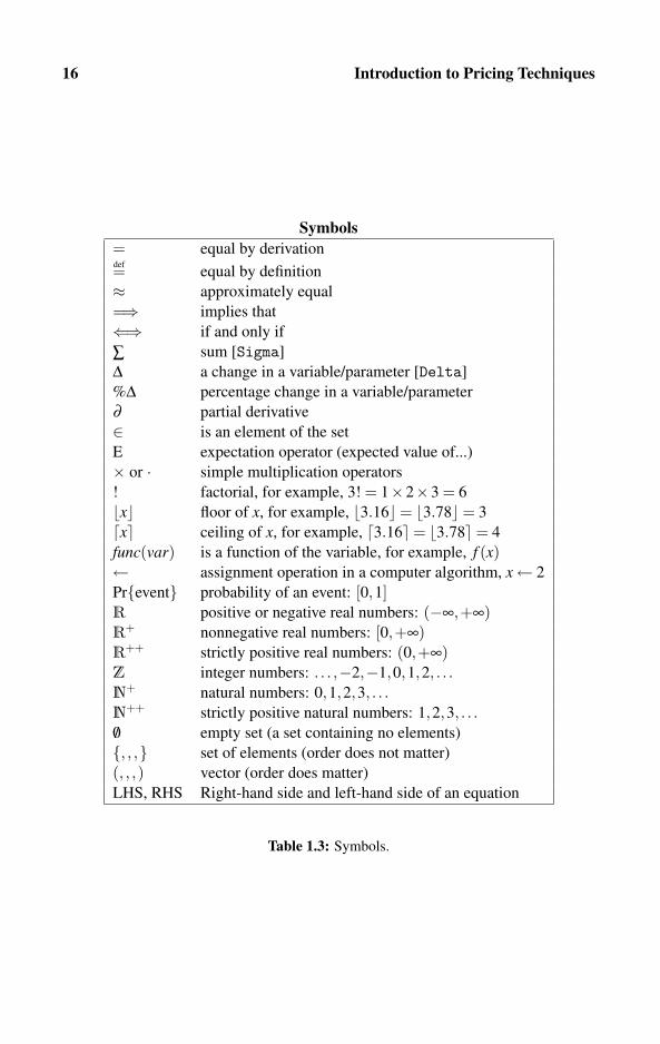
1.8 Notation and Symbols
The book tries to minimize the use of mathematical symbols. For the sake of com-
pleteness, Table 1.3 contains all the symbols used in this book.
Notation is classified into two groups: parameters, which are numbers that are
treated as exogenous by the agents described in the model, and variables, which
1.8 Notation and Symbols 15
are endogenously determined. Thus, the purpose of every theoretical model is to
define an equilibrium concept that yields a unique solution for these variables for
given values of the model’s parameters.
For example, production costs and consumers’ valuations of products are typ-
ically described by parameters (constants), which are estimated in the market by
econometricians and are taken exogenously by the theoretical economist. In con-
trast, quantity produced and quantity consumed are classical examples of variables
that are endogenously determined, meaning that they are solved within the model
itself.
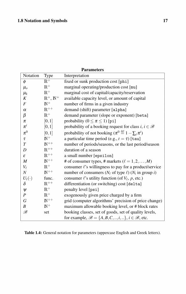
We now set the rule for assigning notation to parameters and variables. Pa-rameters are denoted either by Greek letters or by uppercase English letters. Incontrast, variables are denoted by lowercase English letters. Table 1.4 lists the
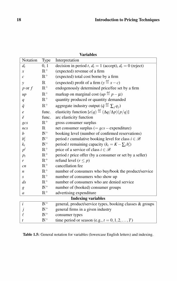
notation used for denoting parameters throughout this book. Finally, Table 1.5 lists
the notation used for denoting variables throughout this book.
16 Introduction to Pricing Techniques
Symbols= equal by derivationdef= equal by definition
≈ approximately equal
=⇒ implies that
⇐⇒ if and only if
∑ sum [Sigma]
Δ a change in a variable/parameter [Delta]
%Δ percentage change in a variable/parameter
∂ partial derivative
∈ is an element of the set
E expectation operator (expected value of...)
× or · simple multiplication operators
! factorial, for example, 3! = 1×2×3 = 6
�x� floor of x, for example, �3.16�= �3.78�= 3
�x ceiling of x, for example, �3.16= �3.78= 4
func(var) is a function of the variable, for example, f (x)← assignment operation in a computer algorithm, x← 2
Pr{event} probability of an event: [0,1]R positive or negative real numbers: (−∞,+∞)R+ nonnegative real numbers: [0,+∞)R++ strictly positive real numbers: (0,+∞)Z integer numbers: . . . ,−2,−1,0,1,2, . . .N+ natural numbers: 0,1,2,3, . . .N++ strictly positive natural numbers: 1,2,3, . . ./0 empty set (a set containing no elements)
{, , ,} set of elements (order does not matter)
(, , ,) vector (order does matter)
LHS, RHS Right-hand side and left-hand side of an equation
Table 1.3: Symbols.
1.8 Notation and Symbols 17
ParametersNotation Type Interpretation
φ R+ fixed or sunk production cost [phi]
μo R+ marginal operating/production cost [mu]
μk R+ marginal cost of capital/capacity/reservation
K R+, N+ available capacity level, or amount of capital
F N+ number of firms in a given industry
α R++ demand (shift) parameter [alpha]
β R+ demand parameter (slope or exponent) [beta]
π [0,1] probability (0≤ π ≤ 1) [pi]
π i [0,1] probability of a booking request for class i, i ∈B
π0 [0,1] probability of not booking (π0 def= 1−∑i π i)
τ N+ a particular time period (e.g., t = τ) [tau]
T N++ number of periods/seasons, or the last period/season
D R++ duration of a season
ε R++ a small number [epsilon]
M N++ # of consumer types, # markets (� = 1,2, . . . ,M)
V� R+ consumer �’s willingness to pay for a product/service
N N++ number of consumers (N� of type �) (Ni in group i)U�(·) func. consumer �’s utility function (of V�, p, etc.)
δ R++ differentiation (or switching) cost [delta]
ψ R+ penalty level [psi]
P R+ exogenously given price charged by a firm
G N++ grid (computer algorithms’ precision of price change)
B N+ maximum allowable booking level, or # block rates
B set booking classes, set of goods, set of quality levels,
for example, B = {A,B,C, .., i, ..}, i ∈B, etc.
Table 1.4: General notation for parameters (uppercase English and Greek letters).
18 Introduction to Pricing Techniques
VariablesNotation Type Interpretation
dt 0, 1 decision in period t, dt = 1 (accept), dt = 0 (reject)
x R+ (expected) revenue of a firm
c R+ (expected) total cost borne by a firm
y R (expected) profit of a firm (y def= x− c)
p or f R+ endogenously determined price/fee set by a firm
up R+ markup on marginal cost (up def= p−μ)
q R+ quantity produced or quantity demanded
q R+ aggregate industry output (q def= ∑ j q j)
e func. elasticity function [e(q) def= (Δq/Δp)(p/q)]e func. arc elasticity function
gcs R+ gross consumer surplus
ncs R net consumer surplus (= gcs− expenditure)
b N+ booking level (number of confirmed reservations)
bit N+ period t cumulative booking level for class i ∈B
kt N+ period t remaining capacity (kt = K−∑i bit)
pi R+ price of a service of class i ∈Bpt R+ period t price offer (by a consumer or set by a seller)
r R+ refund level (r ≤ p)
cn R+ cancellation fee
n R+ number of consumers who buy/book the product/service
s R+ number of consumers who show up
ds R+ number of consumers who are denied service
g N+ number of (booked) consumer groups
a R+ advertising expenditure
Indexing variablesi N+ general, product/service types, booking classes & groups
j N+ general firms in a given industry
� N+ consumer types
t N+ time period or season (e.g., t = 0,1,2, . . . ,T )
Table 1.5: General notation for variables (lowercase English letters) and indexing.

Chapter 2
Demand and Cost
2.1 Demand Theory and Interpretations 202.1.1 Definitions
2.1.2 Interpreting goods and services
2.1.3 The elasticity and revenue functions
2.2 Discrete Demand Functions 242.3 Linear Demand Functions 26
2.3.1 Definition
2.3.2 Estimation of linear demand functions
2.3.3 Elasticity and revenue for linear demand
2.4 Constant-elasticity Demand Functions 302.4.1 Definition and characterization
2.4.2 Estimation of constant-elasticity demand functions
2.4.3 Elasticity and revenue for constant-elasticity demand
2.5 Aggregating Demand Functions 342.5.1 Aggregating single-unit demand functions
2.5.2 Aggregating continuous demand functions
2.6 Demand and Network Effects 392.7 Demand for Substitutes and Complements 422.8 Consumer Surplus 45
2.8.1 Consumer surplus: Discrete demand functions
2.8.2 Consumer surplus: Continuous demand functions
2.9 Cost of Production 522.10 Exercises 56
The key to a successful implementation of any yield management strategy is getting
to know the consumers. Large firms invest tremendous amounts of money on re-
search seeking to characterize their own customers as well as potential consumers.
In economic theory, the most useful instrument for characterizing consumer behav-
ior is the demand function. A demand function shows the quantity demanded by an

20 Demand and Cost
individual, a group, or all the consumers in a given market, as a function of market
prices, and some other variables.
Knowing the demand structure is a necessary condition for proper selection of
profit-maximizing actions by the firm. But it is not a sufficient condition because
the firm must also take cost-of-production considerations into account. Therefore,
price decision makers within a firm should properly study the structure of the cost
of the service or the product sold by their own firms. They should also distinguish
among the different types of costs, particularly between costs associated with a
marginal expansion of output and costs associated with investing in infrastructure,
research and development (R&D), and capacity.
For this reason, we devote an entire chapter to study the most widely used
demand and cost structures. Some readers, particularly readers who took micro-
economics courses at a second-year undergraduate level, may be familiar with this
material. In general, readers can skip this chapter and use it as a reference for the
various concepts whenever necessary.
2.1 Demand Theory and Interpretations
In most cases, knowing consumers’ demands constitutes the key information
on which producers, service providers, and sellers in general base their profit-
maximizing pricing and marketing techniques. However, the concepts of demand,
products, and services may be given a wide variety of interpretations. In this sec-
tion, we discuss some of these interpretations as it is important that firms identify
the precise type of demand they are facing before they design their pricing mecha-
nisms.
2.1.1 DefinitionsDEFINITION 2.1
(a) The demand function q(p) shows the quantity demanded at any given price,
p≥ 0, by a single consumer or a group of consumers.
(b) The inverse demand function p(q) shows the maximum amount that an in-
dividual or a group of individuals is willing to pay at any given consumption
level, q ≥ 0. Mathematically, the function p(q) is the inverse of the function
q(p).
Notice that Definition 2.1 is general enough to be applied to different levels of
market aggregation in the sense that it can be applied to individuals as well as to
different-sized markets. The technique for how to combine individuals’ demand
functions into a single market demand function will be studied in Section 2.5.
Definition 2.1 is incomplete in the sense that it makes the quantity demanded
depend on the price/fee only. However, as the reader may be well aware of, de-
mand is also influenced by a wide variety of other factors, such as prices of other
2.1 Demand Theory and Interpretations 21
goods and services that consumers may view as substitutes or complements, in-
come levels, time of delivery, bundling and tying with other goods and services,
advertising, social conformity and nonconformity, social pressure, network effects,
environmental concerns, brand loyalty, and more. Clearly, all these factors are very
important, and most of them are incorporated in this book.
2.1.2 Interpreting goods and services
This book analyzes profit-maximizing pricing techniques. For this reason, produc-
ers and service providers should fully understand and very often define the nature
of the products and services they supply. Furthermore, it is important that sellers
understand how these products and services are used by consumers and how con-
sumers perceive the benefit they gain from consuming these goods. For this reason,
we now attempt to characterize goods and services according to several criteria.
Frequency of purchase: Flow versus stock goods
The distinction between flow and stock goods is based on the frequency of pur-
chase. Theoretically, pure stock goods are those that can be stored indefinitely.
Diamonds, gold, silver, and artworks are good examples. However, often we view
mechanical and electrical appliances also as stock goods despite the fact that they
tend to be replaced every few years. Flow goods are generally perishable goods for
which the quantity demanded is measured by units of consumption during a certain
time period. By perishable, we mean goods that cannot be stored for a long time,
if at all. Therefore, perishable products must be repeatedly purchased. Food items,
perhaps, provide the best examples of flow goods. Some food items can be stored
for only a week, whereas others (such as boxed food) can be stored for six months
or even longer.
Because the majority of pricing models presented in this book apply to services,
we should mention that services are generally regarded as highly perishable, which
means they are nonstorable. The reason for this is that most services are time
dependent, so postponements and delays may result in a partial or total utility loss
to consumers. For example, traveling today via ground, air, or sea transportation, or
a hotel room for tonight, may be regarded as totally different services from traveling
and a hotel room tomorrow. Reading or watching the news today constitute a totally
different service from getting tomorrow’s news. Of course, this is not always the
case as for some services, such as changing the engine oil in your car, postponing
the service for a limited time will not matter to you very much. Despite the fact
that most services are perishable, not all services are flow goods in the sense that
some services, such as a trip to the Galapagos Islands, may be purchased once in a
lifetime. In contrast, a bus trip to work is definitely a flow good, as it is repeated on
a daily basis. A ski trip can also be repeated on a yearly basis or for some people,
can be a once-in-a-lifetime event.

22 Demand and Cost
Back to products, in the “new” information economy, information goods con-
sume a large portion of individuals’ budgets. We interpret information goods in the
broad sense of the term to include books, software, encyclopedias, databases, mu-
sic, and video. We tend to treat these information products as stock goods. Not only
can these products be stored for a long period of time, they can also be duplicated
without any deterioration if they are stored in digital formats. Of course, storage de-
vices such as magnetic tapes, digital disks, and diskettes, are themselves perishable
and therefore require some maintenance or replacement. We should point out that
in some sense, information goods can also be viewed as services simply because
there is no benefit from storing them. News on current prices in the stock markets,
or any other type of news, can be viewed as perishable goods that consumers must
purchase repeatedly.
Quantity of purchase and willingness to pay
Generally, there are two major interpretations for demand schedules. The first in-
terpretation involves consumers who increase the number of units purchased when
the price drops (holding other parameters affecting demand constant). This in-
terpretation is commonly found in introductory textbooks that are used in univer-
sity microeconomics courses. With the risk of finding many counterexamples, we
can say that this interpretation is more suitable for markets of flow goods, where
frequent purchases make the quantity purchased highly sensitive to short-run and
small changes in prices. Figure 2.1(left) illustrates a downward-sloping inverse
demand function for one individual consumer. Thus, the consumer depicted on
Figure 2.1(left) demands q = 2 units at the price of p = $30, q = 3 units at p = $25,
and so on.
� �
� �
pp
••$30
$25
••
•
$20
$15
$10
2 6 7 93 4 5 81 1
$20
0
•
Figure 2.1: Illustration of inverse demand functions by individuals. Left: Downward-
sloping demand. Right: Single-unit demand.
The second interpretation, which will be used extensively in this book, applies
to markets composed of a large number of individuals. Each consumer is assumed
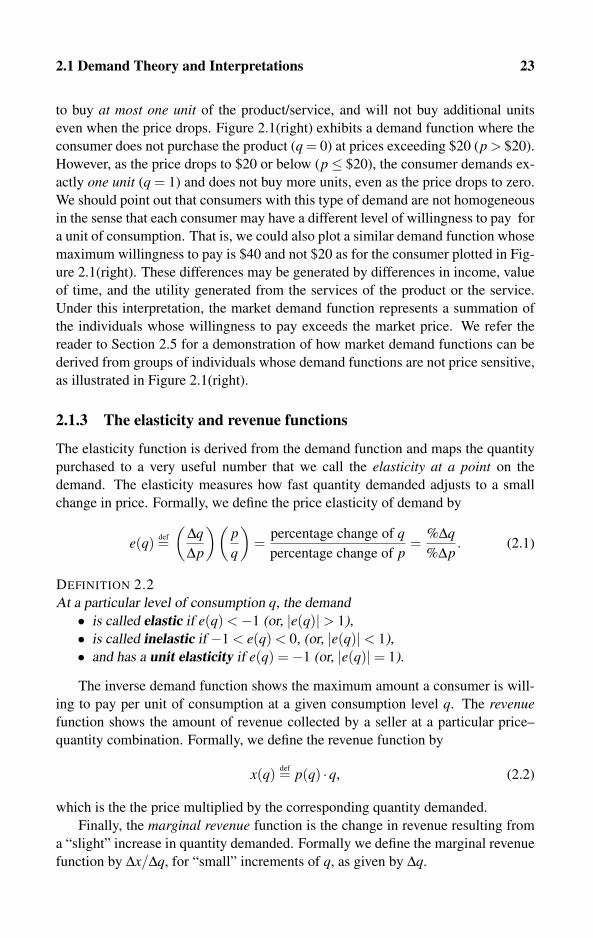
2.1 Demand Theory and Interpretations 23
to buy at most one unit of the product/service, and will not buy additional units
even when the price drops. Figure 2.1(right) exhibits a demand function where the
consumer does not purchase the product (q = 0) at prices exceeding $20 (p > $20).
However, as the price drops to $20 or below (p≤ $20), the consumer demands ex-
actly one unit (q = 1) and does not buy more units, even as the price drops to zero.
We should point out that consumers with this type of demand are not homogeneous
in the sense that each consumer may have a different level of willingness to pay for
a unit of consumption. That is, we could also plot a similar demand function whose
maximum willingness to pay is $40 and not $20 as for the consumer plotted in Fig-
ure 2.1(right). These differences may be generated by differences in income, value
of time, and the utility generated from the services of the product or the service.
Under this interpretation, the market demand function represents a summation of
the individuals whose willingness to pay exceeds the market price. We refer the
reader to Section 2.5 for a demonstration of how market demand functions can be
derived from groups of individuals whose demand functions are not price sensitive,
as illustrated in Figure 2.1(right).
2.1.3 The elasticity and revenue functions
The elasticity function is derived from the demand function and maps the quantity
purchased to a very useful number that we call the elasticity at a point on the
demand. The elasticity measures how fast quantity demanded adjusts to a small
change in price. Formally, we define the price elasticity of demand by
e(q) def=(
ΔqΔp
)(pq
)=
percentage change of qpercentage change of p
=%Δq%Δp
. (2.1)
DEFINITION 2.2
At a particular level of consumption q, the demand
• is called elastic if e(q) <−1 (or, |e(q)|> 1),
• is called inelastic if −1 < e(q) < 0, (or, |e(q)|< 1),
• and has a unit elasticity if e(q) =−1 (or, |e(q)|= 1).
The inverse demand function shows the maximum amount a consumer is will-
ing to pay per unit of consumption at a given consumption level q. The revenuefunction shows the amount of revenue collected by a seller at a particular price–
quantity combination. Formally, we define the revenue function by
x(q) def= p(q) ·q, (2.2)
which is the the price multiplied by the corresponding quantity demanded.
Finally, the marginal revenue function is the change in revenue resulting from
a “slight” increase in quantity demanded. Formally we define the marginal revenue
function by Δx/Δq, for “small” increments of q, as given by Δq.

24 Demand and Cost
2.2 Discrete Demand Functions
Data on demand are discrete in nature because the number of observations in the
form of data points that can be collected is always finite. Therefore, when a re-
searcher plots the raw data, the demand function consists of discrete points in the
price–quantity space. We refer to graphs representing the raw data as discrete de-
mand functions, and distinguish them from the continuous demand functions we
also analyze in this chapter. In fact, in Sections 2.3 and 2.4, we demonstrate how to
generate continuous linear and constant-elasticity demand functions from discrete
demand by estimating the continuous functions directly from the raw data. Al-
though most textbooks in economics use continuous demand functions, this book
focuses mainly on discrete demand functions. The reason is that, by construction,
computers generally handle computations based on a finite amount of data. This
means that the computations based on raw data, or based on data generated by com-
puter reservation systems, must be handled using discrete algebra (as opposed to
calculus).
The first two rows of Table 2.1 display the raw data for a discrete demand
function. Rows 3–6 in this table display various computations derived directly
p $35 $30 $25 $25 $20 $20 $15 $15 $10
q 1 2 3 4 5 6 7 8 9
e(q) −7.00 −3.0 n/d −1.25 n/d −0.67 n/d −0.38 n/a
e(q) −4.33 −2.2 n/d −1 n/d −0.54 n/d −0.29 n/a
x(q) $35 $60 $75 $100 $100 $120 $105 $120 90Δx(q)
Δq $25 $15 $25 $0 $20 −$15 $15 −$30 n/a
Table 2.1: Discrete demand function 〈p,q〉, and the corresponding price elasticity e(q), arc
price elasticity e(q), total revenue x(q), and marginal revenueΔx(q)
Δq . Note: n/d
means not defined (division by 0), n/a means data not available.
from the raw data. Figure 2.2 plots the raw data provided by Table 2.1. The third
row of Table 2.1 computes the price elasticity defined by (2.1). To demonstrate two
examples, we compute the price elasticity at q = 1 and q = 6 units of consumption
to be
e(1) =2−1
$30−$35
$35
1=−7 and e(6) =
7−6
$15−$20
$20
6=−0.67. (2.3)
Observe that we are unable to compute the price elasticity at q = 9, because we
have no data on the price that would induce the consumer(s) to buy q = 10 units.
For this reason, we marked e(9) as n/a in Table 2.1.
Inspecting the elasticity computations given by (2.3) reveals that the elastic-
ity formula is based on the evaluation of the price and the corresponding quan-
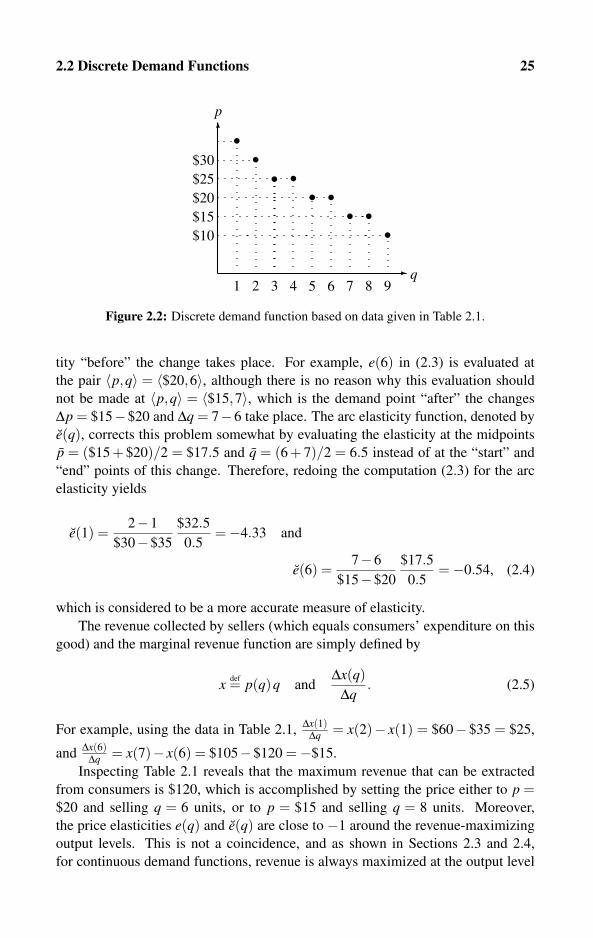
2.2 Discrete Demand Functions 25
�
�
q
p
••$30
$25
••
•
$20
$15
$10
2 6 7 93 4 5 81
•
••
•
Figure 2.2: Discrete demand function based on data given in Table 2.1.
tity “before” the change takes place. For example, e(6) in (2.3) is evaluated at
the pair 〈p,q〉 = 〈$20,6〉, although there is no reason why this evaluation should
not be made at 〈p,q〉 = 〈$15,7〉, which is the demand point “after” the changes
Δp = $15−$20 and Δq = 7−6 take place. The arc elasticity function, denoted by
e(q), corrects this problem somewhat by evaluating the elasticity at the midpoints
p = ($15 + $20)/2 = $17.5 and q = (6 + 7)/2 = 6.5 instead of at the “start” and
“end” points of this change. Therefore, redoing the computation (2.3) for the arc
elasticity yields
e(1) =2−1
$30−$35
$32.5
0.5=−4.33 and
e(6) =7−6
$15−$20
$17.5
0.5=−0.54, (2.4)
which is considered to be a more accurate measure of elasticity.
The revenue collected by sellers (which equals consumers’ expenditure on this
good) and the marginal revenue function are simply defined by
x def= p(q)q andΔx(q)
Δq. (2.5)
For example, using the data in Table 2.1,Δx(1)
Δq = x(2)− x(1) = $60− $35 = $25,
andΔx(6)
Δq = x(7)− x(6) = $105−$120 =−$15.
Inspecting Table 2.1 reveals that the maximum revenue that can be extracted
from consumers is $120, which is accomplished by setting the price either to p =$20 and selling q = 6 units, or to p = $15 and selling q = 8 units. Moreover,
the price elasticities e(q) and e(q) are close to −1 around the revenue-maximizing
output levels. This is not a coincidence, and as shown in Sections 2.3 and 2.4,
for continuous demand functions, revenue is always maximized at the output level

26 Demand and Cost
where both elasticities take a value of e(q) = e(q) = −1. Observe that regular
and arc elasticities are always equal for continuous demand functions because their
evaluation is based on infinitesimal changes.
2.3 Linear Demand Functions
2.3.1 Definition
A linear demand is a special type of the general demand function characterized by
Definition 2.1. Its special property is that it is drawn as, or fitted to be represented
by, a straight line. Formally, the general formulas for the inverse and the direct
demand functions are defined by
p(q) def= α−β q or q(p) def=αβ− 1
βp, (2.6)
where the parameters α and β may be estimated using econometric techniques, as
we briefly demonstrate in Section 2.3.2. Figure 2.3 plots the linear inverse demand
function given by the formula on the left-hand side of (2.6). Note that part of the
�
�
q
α
α2β
elastic: |e|> 1
inelastic: |e|< 1
unit elasticity: |e|= 1
���
p
p(q) = α−β q
ΔxΔq = α−2βq
αβ
Figure 2.3: Inverse linear demand function.
demand is not drawn in Figure 2.3. That is, for any price exceeding the intercept
α , the (inverse) demand becomes vertical at q = 0. In other words, the demand
coincides with the vertical axis for prices in the range p > α .
For the inverse demand function, the parameter α > 0 is called the demand
intercept, whereas the parameter β ≥ 0 is called the slope of the inverse demand
curve. We should mention that in rare cases, −β may be found to have a positive
slope for some price range. Inverting the inverse demand function formulated on
the left-hand side of (2.6) generates the direct demand function on the right-hand
side of (2.6), with an intercept α/β and a slope of −1/β .

2.3 Linear Demand Functions 27
2.3.2 Estimation of linear demand functions
Firms can collect data on the demand facing their products and services by ex-
perimenting with different prices and recording the quantity demanded at every
price. Alternatively, firms can conduct consumer surveys. What is common to
both methods is that the data collected are discrete (as opposed to continuous). In
other words, observations generally consist of data points that are a collection of
the pairs 〈p,q〉. Table 2.2 provides an example of data points on quantity demanded
at various prices.
� (observation no.) 1 2 3 4 5 Mean
p� (price) $30 $25 $20 $15 $10 $20.00
q� (quantity) 2 3 6 7 9 5.40
Table 2.2: Data points for estimating linear demand.
The discrete data on price and quantity observations provided by Table 2.2 may
often be hard to use for analyzing pricing techniques. That is, some pricing tactics
are easier to configure when the demand is represented by a continuous function.
We therefore would like to fit a formula that would approximate the behavior of
the consumer whose preferences are represented by the data given in Table 2.2.
Figure 2.4 illustrates how a linear regression line can be fit to approximate the
linear demand function. In fact, using the data in Table 2.2, regressing q on pyields the direct demand function
q = 12.6−0.36 p, or, in an inverted form, p = 35−2.7777q. (2.7)
�
p
••$30
$25
••
•
$20
$15
$10
2 6 73 4 5 81 109 11 12�
13
$35
q
q(p) = 12.6−0.36q
Figure 2.4: Fitting a linear regression line.
Note that regressing q (the dependent variable) on p (an independent vari-
able) is different from regressing p on q. In fact, regressing p on q yields p =
28 Demand and Cost
34.63855−2.71084q, which is somewhat different from the inverse demand func-
tion (2.7) obtained from the estimation of the direct demand function. Unfortu-
nately, there is no easy way to reconcile the two estimation methods. Given that
our computations rely on frequent inversions of direct demand functions into in-
verse demand functions, and the other way around, in this chapter we always es-
timate the direct demand function equation, and then derive the inverse demand
function from the estimated direct demand equation.
The estimated demand function (2.7) is drawn in Figure 2.4. The linear re-
gression yielding the demand schedule (2.7) from the data given in Table 2.2 can
be computed on basically any personal computer that runs a popular spreadsheet
program, or a commonly used statistical package. Most widely used spreadsheet
programs allow users to type in the observed data points then highlight the relevant
rows or columns and obtain the intercept and slope of the demand function. In fact,
some of these packages even draw the regression line with the data points, just as
we did in Figure 2.4. Therefore, there is no need for us to go into detail about
how to derive the formulas for obtaining the intercept and the slope. For the sake
of completeness, we merely add a few remarks on the regression fitting technique.
In general, regression is a statistical technique of fitting a functional relationship
among economic variables by cataloging the observed variables, and then using
well-known formulas to extract the exogenous parameters of the functional rela-
tionship. The most commonly used regression method is known as ordinary least
squares (a method that minimizes the sum of squared errors). Let M be the number
of observations in hand (M = 5 in the example given in Table 2.2). Then, define the
mean price (or average price) and mean quantity demanded (or average quantity)
by
p def=p1 + p2 + · · ·+ pM
M= ∑M
�=1 p�
Mand q def= ∑M
�=1 q�
M. (2.8)
Under the ordinary least squares method, the slope of the direct demand function
q(p) = γ−δ p and its intercept with the horizontal q-axis are obtained from
δ =−∑M�=1(q�− q)(p�− p)
∑M�=1(p�− p)2
and γ = q+δ p. (2.9)
Again, it may not be practical to use (2.9) directly to compute that δ = 0.36 and
γ = 12.6 as given in (2.7), because linear regressions can be computed on most
spreadsheet programs, statistical packages, and even some freely available Web
pages.
2.3.3 Elasticity and revenue for linear demand
The elasticity and revenue functions defined in Section 2.1.3 for the general case
can be easily derived for the linear demand function given by (2.6). Using calculus,

2.3 Linear Demand Functions 29
we obtain
e(q) =dq(p)
dppq
=(− 1
β
)(α−βq
q
)= 1− α
βq. (2.10)
Therefore, the demand has a unit elasticity at the consumption level q = α/(2β ).Consequently, according to Definition 2.2, the demand is elastic at output levels
q < α/(2β ) and is inelastic for q > α/(2β ). The elasticity regions for the linear
demand case are illustrated in Figure 2.3.
The total revenue function associated with the linear demand function (2.6) is
derived as follows:
x(q) = p(q)q = αq−βq2. (2.11)
Hence, using calculus, the marginal revenue function is given by
dx(q)dq
=d[p(q)q]
dq= α−2βq. (2.12)
The total and marginal revenue functions (2.11) and (2.12) are drawn in Figure 2.5.
�
�
qα2β Δx
Δq = α−2βq
αβ
inelastic: |e|< 1elastic: |e|> 1
α
α2
4β
$
x(q) = αq−βq2
Figure 2.5: Total and marginal revenue functions for linear demand.
Comparing the marginal revenue function (2.12) with the inverse demand func-
tion (2.6) reveals that the marginal revenue function has the same intercept α and
twice the negative slope of the inverse demand function. This comparison can be
easily visualized by comparing Figure 2.3 with Figure 2.5, which illustrates a linear
marginal revenue function that intersects the quantity axis at α/2β , which equals
half of α/β (the quantity at the intersection with the demand function). As also
shown in Figure 2.5, revenue is maximized when the firm sells q = α/(2βq) units
where the demand elasticity is e(α/2β ) =−1, or in absolute value |e(α/2β )|= 1.
Finally, you probably have noticed already that the demand elasticity and the
marginal revenue functions are related. That is, Figures 2.3 and 2.5 illustrate that
Δx/Δq = 0 when e(q) = 1, and Δx/Δq > 0 whenever |e(q)|> 1. In fact, as it turns
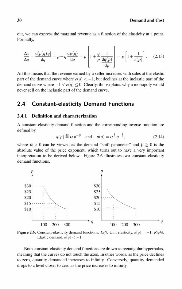
30 Demand and Cost
out, we can express the marginal revenue as a function of the elasticity at a point.
Formally,
ΔxΔq
=d[p(q)q]
dq= p+q
dp(q)dq
= p
⎡⎢⎢⎣1+
qp
1
dq(p)dp
⎤⎥⎥⎦= p
[1+
1
e(p)
]. (2.13)
All this means that the revenue earned by a seller increases with sales at the elastic
part of the demand curve where e(q) <−1, but declines at the inelastic part of the
demand curve where −1 < e(q)≤ 0. Clearly, this explains why a monopoly would
never sell on the inelastic part of the demand curve.
2.4 Constant-elasticity Demand Functions
2.4.1 Definition and characterization
A constant-elasticity demand function and the corresponding inverse function are
defined by
q(p) def= α p−β and p(q) = α1β q−
1β , (2.14)
where α > 0 can be viewed as the demand “shift-parameter” and β ≥ 0 is the
absolute value of the price exponent, which turns out to have a very important
interpretation to be derived below. Figure 2.6 illustrates two constant-elasticity
demand functions.
� �
� �
pp
$30
$25
$20
$15
$10
100 300200
$30
$25
$20
$15
$10
100 300200
Figure 2.6: Constant-elasticity demand functions. Left: Unit elasticity, e(q) =−1. Right:Elastic demand, e(q) <−1.
Both constant-elasticity demand functions are drawn as rectangular hyperbolas,
meaning that the curves do not touch the axes. In other words, as the price declines
to zero, quantity demanded increases to infinity. Conversely, quantity demanded
drops to a level closer to zero as the price increases to infinity.
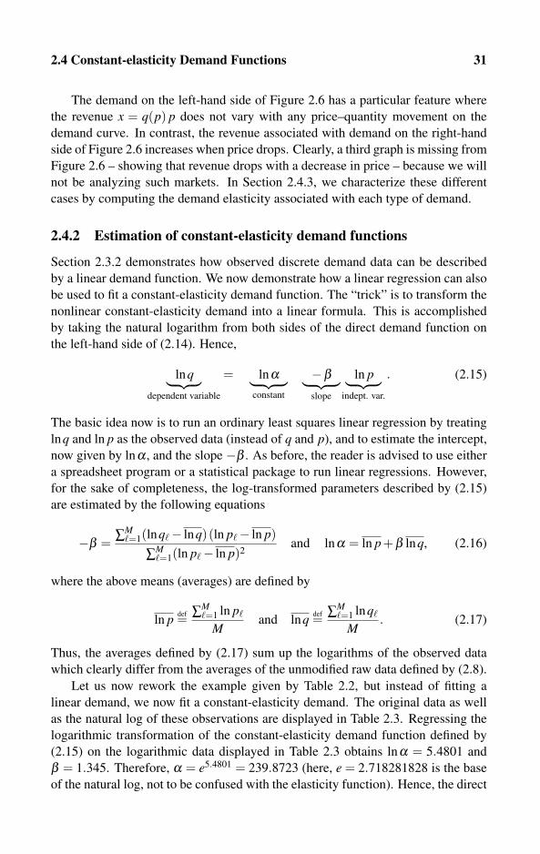
2.4 Constant-elasticity Demand Functions 31
The demand on the left-hand side of Figure 2.6 has a particular feature where
the revenue x = q(p) p does not vary with any price–quantity movement on the
demand curve. In contrast, the revenue associated with demand on the right-hand
side of Figure 2.6 increases when price drops. Clearly, a third graph is missing from
Figure 2.6 – showing that revenue drops with a decrease in price – because we will
not be analyzing such markets. In Section 2.4.3, we characterize these different
cases by computing the demand elasticity associated with each type of demand.
2.4.2 Estimation of constant-elasticity demand functions
Section 2.3.2 demonstrates how observed discrete demand data can be described
by a linear demand function. We now demonstrate how a linear regression can also
be used to fit a constant-elasticity demand function. The “trick” is to transform the
nonlinear constant-elasticity demand into a linear formula. This is accomplished
by taking the natural logarithm from both sides of the direct demand function on
the left-hand side of (2.14). Hence,
lnq︸ ︷︷ ︸dependent variable
= lnα︸ ︷︷ ︸constant
−β︸ ︷︷ ︸slope
ln p︸ ︷︷ ︸indept. var.
. (2.15)
The basic idea now is to run an ordinary least squares linear regression by treating
lnq and ln p as the observed data (instead of q and p), and to estimate the intercept,
now given by lnα , and the slope −β . As before, the reader is advised to use either
a spreadsheet program or a statistical package to run linear regressions. However,
for the sake of completeness, the log-transformed parameters described by (2.15)
are estimated by the following equations
−β = ∑M�=1(lnq�− lnq)(ln p�− ln p)
∑M�=1(ln p�− ln p)2
and lnα = ln p+β lnq, (2.16)
where the above means (averages) are defined by
ln p def= ∑M�=1 ln p�
Mand lnq def= ∑M
�=1 lnq�
M. (2.17)
Thus, the averages defined by (2.17) sum up the logarithms of the observed data
which clearly differ from the averages of the unmodified raw data defined by (2.8).
Let us now rework the example given by Table 2.2, but instead of fitting a
linear demand, we now fit a constant-elasticity demand. The original data as well
as the natural log of these observations are displayed in Table 2.3. Regressing the
logarithmic transformation of the constant-elasticity demand function defined by
(2.15) on the logarithmic data displayed in Table 2.3 obtains lnα = 5.4801 and
β = 1.345. Therefore, α = e5.4801 = 239.8723 (here, e = 2.718281828 is the base
of the natural log, not to be confused with the elasticity function). Hence, the direct

32 Demand and Cost
� (observation no.) 1 2 3 4 5 Mean
p� (price) $30 $25 $20 $15 $10 $20.00
ln p� (log price) 3.40 3.22 3.00 2.71 2.30 2.93
q� (quantity) 2 3 6 7 9 5.40
lnq� (quantity) 0.69 1.10 1.79 1.95 2.20 1.55
Estimated q�(p�) 2.47 3.16 4.27 6.28 10.84 5.40
Table 2.3: Data points for estimating constant-elasticity demand.
and associated inverse estimated constant-elasticity demand functions based on the
observations in Table 2.3 are given by
q(p) = 239.87 p−1.345 or, in an inverted form, p(q) = 58.82q−0.743. (2.18)
Again, note that the inverse demand function on the right-hand side of (2.18) is
not an estimated function but a function derived from the estimated direct demand
equation. As we remarked on the linear case, regressing lnq on ln p and inverting it
need not yield the same result as regressing ln p on lnq. Therefore, for the purpose
of this chapter, we always estimate the direct demand function first, and then invert
it, taking into consideration the possible error. Furthermore, note that there are
some alternative methods for estimating constant-elasticity demand functions that
depend on the specification of the error term.
The estimated quantity levels for each price observation are written on the bot-
tom row of Table 2.3. For example, the observed quantity demanded at the price
p = $30 was q = 2, but the estimated constant-elasticity demand function (2.18)
predicts q = 2.47. Notice that the sampled average quantity demanded and the
estimated average are the same, q = 5.4.
Figure 2.7 plots the inverse demand function from the formula displayed on
the right-hand side of (2.18). This formula yields p(2) = $35.13 > $30, p(3) =$25.99 > $25, p(6) = $15.52 < $20, p(7) = $13.84 < $15, and p(9) = $11.48 >$10. Figure 2.7 also compares the constant-elasticity estimated demand given by
(2.18) to the estimated linear demand given by (2.7) on the same graph. A deeper
comparison between the two fitted functions would require the use of a regression
analysis tool such as the measure of correlation, known as R2, and the p–value.
These are beyond the scope of this book but can be found in any econometrics
textbook as well as on some Web sites.
2.4.3 Elasticity and revenue for constant-elasticity demand
Although constant-elasticity demand functions are more difficult to draw compared
with linear demand functions, they have some useful features that make revenue and
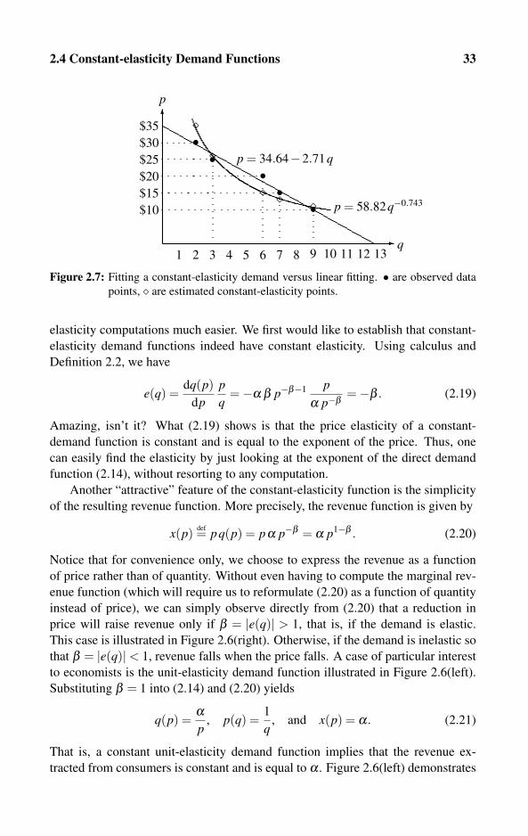
2.4 Constant-elasticity Demand Functions 33
�
p
••$30
$25
••
•
$20
$15
$10
2 6 73 4 5 81 109 11 12�
13
$35
q
p = 34.64−2.71q
�
�
� � � p = 58.82q−0.743
Figure 2.7: Fitting a constant-elasticity demand versus linear fitting. • are observed data
points, � are estimated constant-elasticity points.
elasticity computations much easier. We first would like to establish that constant-
elasticity demand functions indeed have constant elasticity. Using calculus and
Definition 2.2, we have
e(q) =dq(p)
dppq
=−α β p−β−1 pα p−β =−β . (2.19)
Amazing, isn’t it? What (2.19) shows is that the price elasticity of a constant-
demand function is constant and is equal to the exponent of the price. Thus, one
can easily find the elasticity by just looking at the exponent of the direct demand
function (2.14), without resorting to any computation.
Another “attractive” feature of the constant-elasticity function is the simplicity
of the resulting revenue function. More precisely, the revenue function is given by
x(p) def= pq(p) = pα p−β = α p1−β . (2.20)
Notice that for convenience only, we choose to express the revenue as a function
of price rather than of quantity. Without even having to compute the marginal rev-
enue function (which will require us to reformulate (2.20) as a function of quantity
instead of price), we can simply observe directly from (2.20) that a reduction in
price will raise revenue only if β = |e(q)| > 1, that is, if the demand is elastic.
This case is illustrated in Figure 2.6(right). Otherwise, if the demand is inelastic so
that β = |e(q)|< 1, revenue falls when the price falls. A case of particular interest
to economists is the unit-elasticity demand function illustrated in Figure 2.6(left).
Substituting β = 1 into (2.14) and (2.20) yields
q(p) =αp
, p(q) =1
q, and x(p) = α. (2.21)
That is, a constant unit-elasticity demand function implies that the revenue ex-
tracted from consumers is constant and is equal to α . Figure 2.6(left) demonstrates

34 Demand and Cost
that a fall in price is compensated by an exact proportional increase in quantity
demanded. Thus, the revenue equals $9000 at all price levels.
The estimated constant-elasticity demand function drawn in Figure 2.7 has a
price elasticity of |e(p)| = |1.345| > 1, meaning that the demand is elastic, hence
any price reduction would result in higher revenue extracted from consumers. This
is in contrast to the linear demand, for which there is always a price level below
which the demand becomes inelastic.
2.5 Aggregating Demand Functions
In this section, we learn how to combine individual consumers’ demand functions
into a single market demand function faced by firms. We distinguish between two
representations of demand functions. Section 2.5.1 shows how to aggregate dis-
crete single-unit demand functions. This procedure is most suitable for computers
because it involves summations over discrete numbers. Section 2.5.2 shows how
to aggregate continuous demand functions, which are represented by algebraic for-
mulas. We also show how to implement this aggregation procedure on a computer.
2.5.1 Aggregating single-unit demand functions
Section 2.1.2 has already proposed two interpretations for demand functions. Un-
der one interpretation, which is extensively used in this book, market demand is
viewed as a composition of many consumers, each demanding at most one unit.
This interpretation does not rule out the possibility that consumers may differ in
their willingness to pay for a unit of consumption. In this section, we demonstrate
how to combine these individual demand functions into a single market demand
function. This procedure is very important because this aggregation generates dis-
crete market demand functions in the form we have already analyzed in Section 2.2.
The resulting aggregate market demand becomes handy when one wishes to use a
computer to implement profitable pricing techniques.
Figure 2.8 illustrates how different consumer groups (groups combined of indi-
viduals with the same willingness to pay) can be aggregated to form an aggregate
market demand function. The left-hand side of Figure 2.8 illustrates the demand
functions of three representative consumers with different levels of willingness to
pay. Each consumer buys at most one unit (at a given time period, say). For-
mally, they are N1 = 200 consumers, with a maximum willingness to pay of $30;
N2 = 600, whose maximum willingness to pay is $20; and N3 = 200, whose maxi-
mum willingness to pay is $10. The right-hand side illustrates the aggregate market
demand function faced by the firm.
The technique used to aggregate demand functions is known as horizontal sum-mation of demand functions. We use this technique in the computer algorithm that
follows. The idea is to start with a high price exceeding the maximum willingness

2.5 Aggregating Demand Functions 35
�
p
$30
$25
$20
$15
$10
� q1
�
p
$30
$25
$20
$15
$10
� q2
�
p
$30
$25
$20
$15
$10
� q31 1 1
•
•
•
�
p
$30
$25
$20
$15
$10
N1 = 200 N2 = 600 N3 = 200
� q200 400 600 800 1000
•
•
•
Figure 2.8: Aggregating the single-unit demand functions of three consumer types.
to pay of all consumer types. Then, gradually lowering the price induces more
and more consumers to enter the market, where each newly entering consumer pur-
chases one unit. More precisely, at any price p > $30 aggregate demand is q = 0.
At the price range $20 < p ≤ $30, there are exactly N1 = 200 consumers buy-
ing a total of q = 200 units. At the price range $10 < p ≤ $20, there are exactly
N1 +N2 = 200+600 consumers buying a total of q = 800 units. At prices satisfy-
ing p ≤ $10, N1 + N2 + N3 = 200 + 600 + 200 consumers buy a total of q = 1000
units. Finally, the reader can easily confirm that the maximum revenue that can be
extracted from consumers is given by the price–quantity pair p = $20 and q = 800,
yielding a revenue of y(800) = $1600.
Algorithm 2.1 relies on some parameters that the software must input, and some
output variables that should be defined. First, the program should input the number
of consumer types M. Next, for each consumer type �, the software must input
the type’s maximum willingness to pay V [�] and the number of consumers of this
type N[�]. One can construct a loop such as Read(�); 1≤ �≤M, until, say, an end
of line is reached, assuming that each pair of data points consisting of maximum
willingness to pay and the number of consumers of this type ends with an end-
of-line character. Hence, the program should define a real-valued array V [�] of
dimension M + 1, and a nonnegative natural numbers array N[�] of dimension M.
V [M +1] is an ad hoc parameter defined solely for the sake of convenience. Finally,
the software must sort consumer types according to declining willingness to pay.
Formally, Algorithm 2.1 will rely on the assumption that consumers are ordered so
that their maximum willingness to pay satisfies V [1]≥V [2]≥ ·· · ≥V [M].
We now proceed to define the output variables of Algorithm 2.1. Given that
there are M consumer types, there are M internal kinks on the market demand
curve; see Figure 2.8 for an example of M = 3 consumer types. We therefore
define an output (M + 1)-dimensional array q[�] of nonnegative natural numbers

36 Demand and Cost
for the aggregate quantity demanded. q[0] is an ad hoc variable defined merely for
the sake of convenience.
V [M +1]← 0; q[0]← 0; /* Defining ad hoc consumer types */for � = 1 to M do
q[�]← N[�]+ q[�−1]; /* Loop over consumer types */writeln (“At the price range ”, V [�+1], “< p≤ ”, V [�], “aggregate
quantity demanded is q = ”, q[�]);
Algorithm 2.1: Aggregating single-unit demand functions.
Algorithm 2.1 is rather straightforward. It runs a loop from the valuation of
the highest type to the lowest valuation type, � = 1,2, · · · ,M, and for each type it
adds the number of consumers of this type N[�] to the number of consumers who
have higher valuations, given by q[�− 1]. Note that just for the sake of complete-
ness, we could define an additional M-dimensional output array p[�] of prices that
would correspond to the aggregate demand levels q[�]. However, this is redundant
given that we merely assign valuations to prices in the form of p[�]←V [�] for each
consumer type � = 1,2, . . . ,M.
2.5.2 Aggregating continuous demand functions
Using software for symbolic algebra, computers can also handle formulas. Contin-
uous demand functions can be constructed by fitting these functions using discrete
observed data points, as we have already demonstrated in Sections 2.3.2 and 2.4.2.
Continuous functions can take the form of a linear function (straight lines as in
Figure 2.3) or of nonlinear functions (as illustrated in Figure 2.6).
Aggregating linear demand functions
We now demonstrate how to aggregate linear demand functions. The aggregation
method for adding the inverse demand functions drawn in Figure 2.9 is commonly
called horizontal summation. This method involves starting at a price high enough
so the quantity demanded is zero then gradually reducing the price and adding
quantity demanded from all markets with strictly positive demand. For example,
in Figure 2.9, q = q1 +q2 = 0+0 for all prices p≥ $30. For all prices $20≤ p <$30, q = q1 +0, hence at this price range the aggregate demand function coincides
with the demand function of market 1 only. For prices in the range 0 ≤ p < $20,
q = q1 +q2 as illustrated on the right-hand side of Figure 2.9. Thus, the aggregate
demand function exhibits a kink each time the price drops below the level that
induces consumers in a new market to enter the market and make purchases. If
we were to add three demand functions (instead of two), we would have two kinks
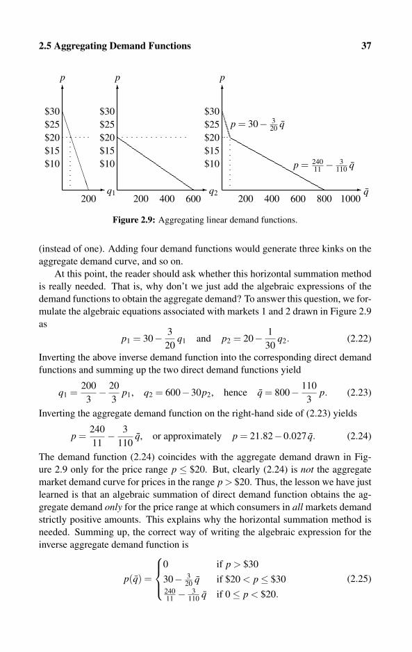
2.5 Aggregating Demand Functions 37
�
p
$30
$25
$20
$15
$10
�
p
$30
$25
$20
$15
$10
�
p
$30
$25
$20
$15
$10
� q200 400 600 800 1000
� �q1 q2200
���������
200 400 600
p = 24011− 3
110q
p = 30− 320
q
Figure 2.9: Aggregating linear demand functions.
(instead of one). Adding four demand functions would generate three kinks on the
aggregate demand curve, and so on.
At this point, the reader should ask whether this horizontal summation method
is really needed. That is, why don’t we just add the algebraic expressions of the
demand functions to obtain the aggregate demand? To answer this question, we for-
mulate the algebraic equations associated with markets 1 and 2 drawn in Figure 2.9
as
p1 = 30− 3
20q1 and p2 = 20− 1
30q2. (2.22)
Inverting the above inverse demand function into the corresponding direct demand
functions and summing up the two direct demand functions yield
q1 =200
3− 20
3p1, q2 = 600−30p2, hence q = 800− 110
3p. (2.23)
Inverting the aggregate demand function on the right-hand side of (2.23) yields
p =240
11− 3
110q, or approximately p = 21.82−0.027 q. (2.24)
The demand function (2.24) coincides with the aggregate demand drawn in Fig-
ure 2.9 only for the price range p ≤ $20. But, clearly (2.24) is not the aggregate
market demand curve for prices in the range p > $20. Thus, the lesson we have just
learned is that an algebraic summation of direct demand function obtains the ag-
gregate demand only for the price range at which consumers in all markets demand
strictly positive amounts. This explains why the horizontal summation method is
needed. Summing up, the correct way of writing the algebraic expression for the
inverse aggregate demand function is
p(q) =
⎧⎪⎨⎪⎩
0 if p > $30
30− 320
q if $20 < p≤ $3024011− 3
110q if 0≤ p < $20.
(2.25)

38 Demand and Cost
Aggregating nonlinear continuous demand functions
Once the principle of the horizontal summation method is understood, it can be ap-
plied to aggregating all types of demand functions, including nonlinear as well as
discontinuous demand functions. This means that there is no need to develop any
new tool for aggregating nonlinear continuous functions. This section is included
here mainly for the sake of completeness, as no new tools will be developed. Fig-
ure 2.10 provides an example of aggregating two constant-elasticity demand func-
tions. The double-arrow lines indicate how horizonal summation is implemented.
At any given price, one should simply add the horizonal distance q1 to q2 (and other
additional markets, if any) to obtain the aggregate demand at a particular price.
�
p�
p
� q� q2
�
p
q1�
���� �� ��
Figure 2.10: Aggregating constant-elasticity demand functions using the horizonal sum-mation method.
Algebraically, suppose that we start with M direct constant elasticity demand
functions as defined by (2.14). Then, the aggregate demand is found by the simple
summation
q = α1 p−β1 +α2 p−β2 + · · ·+αM p−βM . (2.26)
This summation is valid for all nonnegative prices because constant-elasticity de-
mand functions do not “touch the axes,” so there is no danger of summing up nega-
tive output levels. Clearly, at this level of generality we cannot invert the aggregate
demand function. This should not pose a problem because we can still plot the di-
rect demand function by flipping the axes in Figure 2.10 so that aggregate quantity
is measured on the vertical axis instead of the horizontal axis.
One particular case in which we can invert the aggregate demand function is
worth examining. Suppose that all price elasticities are estimated to be approxi-
mately the same among all consumers. That is, if β = β1 = · · ·= βM, we can invert
the direct aggregate demand (2.26) to obtain the aggregate inverse demand function
given by
p(q) =(
qα1 +α2 + · · ·+αM
)− 1β
=(
q
∑M�=1 α�
)− 1β
, (2.27)
2.6 Demand and Network Effects 39
which can be plotted directly on the inverse demand space as illustrated in Fig-
ure 2.10.
Computer algorithm for continuous demand
Because we are dealing now with continuous demand functions that are repre-
sentable by algebraic formulas, it may be more beneficial to use symbolic algebra
software to sum up these equations. However, as illustrated earlier for the linear
case, when summing up formulas, one must be careful not to add negative output
levels. Clearly, this problem can be avoided provided that the formulas are properly
defined by the computer program so that the “kinks” are recognized.
If a symbolic algebra software solution is not an option, or if the researcher
wishes to plot the aggregate demand function, in which case a continuous demand
function must be transformed into a discrete demand, the following algorithm may
be useful. Algorithm 2.2 is rather straightforward. It runs a loop on prices using
a precision chosen by the user, and adds the quantity demanded (after checking
for nonnegativity) from all user-defined (or user-inputted) types of direct demand
functions. The software should input the parameter M which is the number of
different demand functions. Then, either the user defines or the program inputs
(this may be complicated if demand functions are of very different types) an ar-
ray of M direct demand functions: Quant(p)[1], Quant(p)[2], . . . , Quant(p)[M].To make this algorithm more general than the examples illustrated by Figures 2.9
and 2.10, the following algorithm can accommodate an arbitrary number of con-
sumers of each type, where each type can be represented by a different demand
function. Formally, the program should input the number of type � consumers hav-
ing the demand function Quant(p)[�] into N[�], where N[1], . . . ,N[M] is an array
of nonnegative natural numbers. It should also input the desired price range pmin
and pmax, where pmax > pmin ≥ 0, as well as the grid G ∈N++, which determines
the precision (number of points) for the outputted aggregate demand. Δp will serve
as the variable of the price change between data points, determined by the grid
parameter G.
2.6 Demand and Network Effects
So far, our analysis was confined to consumers whose demand functions were in-
dependent of consumption choices made by other consumers. However, it is often
observed that consumers’ choices of what and how much to consume (and at what
price) are influenced by the choices made by other consumers. There can be two
reasons for that. The first is a psychological reason stemming from social pres-
sure either to look like everybody else or to look very different from everyone else.
Second, as we demonstrate below, the demand for telecommunication services de-
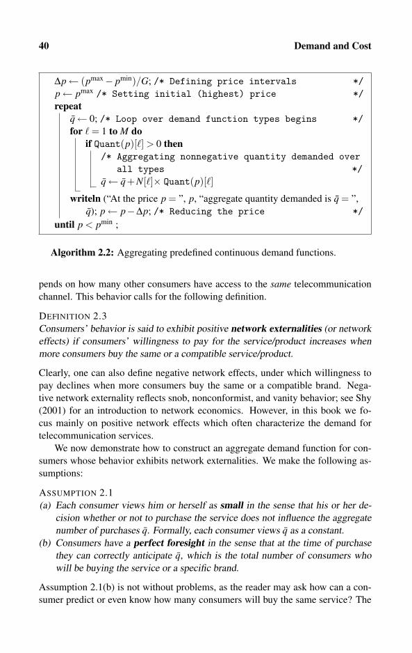
40 Demand and Cost
Δp← (pmax− pmin)/G; /* Defining price intervals */p← pmax /* Setting initial (highest) price */repeat
q← 0; /* Loop over demand function types begins */for � = 1 to M do
if Quant(p)[�] > 0 then/* Aggregating nonnegative quantity demanded over
all types */q← q+N[�]× Quant(p)[�]
writeln (“At the price p = ”, p, “aggregate quantity demanded is q = ”,
q); p← p−Δp; /* Reducing the price */
until p < pmin ;
Algorithm 2.2: Aggregating predefined continuous demand functions.
pends on how many other consumers have access to the same telecommunication
channel. This behavior calls for the following definition.
DEFINITION 2.3
Consumers’ behavior is said to exhibit positive network externalities (or network
effects) if consumers’ willingness to pay for the service/product increases when
more consumers buy the same or a compatible service/product.
Clearly, one can also define negative network effects, under which willingness to
pay declines when more consumers buy the same or a compatible brand. Nega-
tive network externality reflects snob, nonconformist, and vanity behavior; see Shy
(2001) for an introduction to network economics. However, in this book we fo-
cus mainly on positive network effects which often characterize the demand for
telecommunication services.
We now demonstrate how to construct an aggregate demand function for con-
sumers whose behavior exhibits network externalities. We make the following as-
sumptions:
ASSUMPTION 2.1
(a) Each consumer views him or herself as small in the sense that his or her de-
cision whether or not to purchase the service does not influence the aggregate
number of purchases q. Formally, each consumer views q as a constant.
(b) Consumers have a perfect foresight in the sense that at the time of purchase
they can correctly anticipate q, which is the total number of consumers who
will be buying the service or a specific brand.
Assumption 2.1(b) is not without problems, as the reader may ask how can a con-
sumer predict or even know how many consumers will buy the same service? The
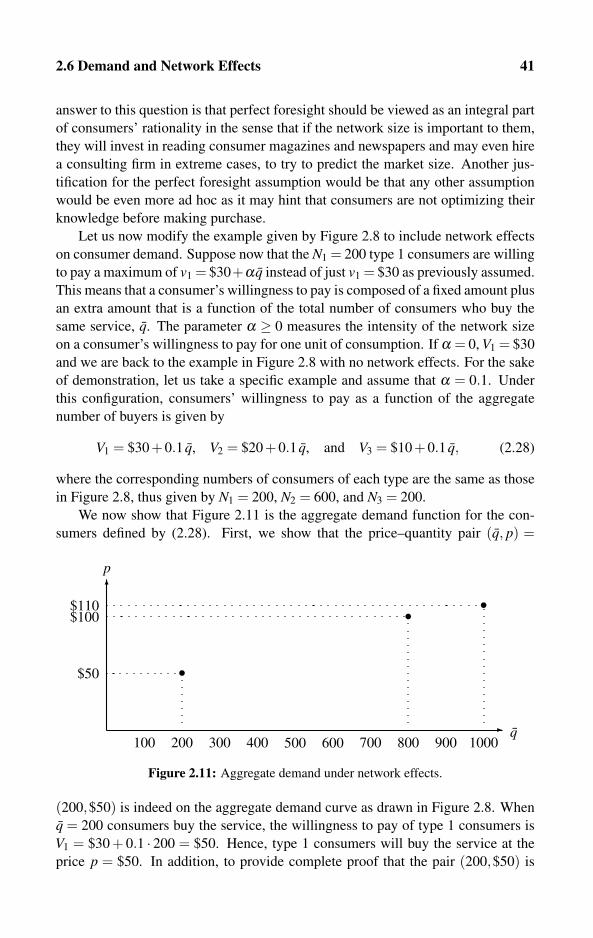
2.6 Demand and Network Effects 41
answer to this question is that perfect foresight should be viewed as an integral part
of consumers’ rationality in the sense that if the network size is important to them,
they will invest in reading consumer magazines and newspapers and may even hire
a consulting firm in extreme cases, to try to predict the market size. Another jus-
tification for the perfect foresight assumption would be that any other assumption
would be even more ad hoc as it may hint that consumers are not optimizing their
knowledge before making purchase.
Let us now modify the example given by Figure 2.8 to include network effects
on consumer demand. Suppose now that the N1 = 200 type 1 consumers are willing
to pay a maximum of v1 = $30+α q instead of just v1 = $30 as previously assumed.
This means that a consumer’s willingness to pay is composed of a fixed amount plus
an extra amount that is a function of the total number of consumers who buy the
same service, q. The parameter α ≥ 0 measures the intensity of the network size
on a consumer’s willingness to pay for one unit of consumption. If α = 0, V1 = $30
and we are back to the example in Figure 2.8 with no network effects. For the sake
of demonstration, let us take a specific example and assume that α = 0.1. Under
this configuration, consumers’ willingness to pay as a function of the aggregate
number of buyers is given by
V1 = $30+0.1 q, V2 = $20+0.1 q, and V3 = $10+0.1 q, (2.28)
where the corresponding numbers of consumers of each type are the same as those
in Figure 2.8, thus given by N1 = 200, N2 = 600, and N3 = 200.
We now show that Figure 2.11 is the aggregate demand function for the con-
sumers defined by (2.28). First, we show that the price–quantity pair (q, p) =
�
�
100 200 300 400 500 600 700 800 1000900q
p
$100$110
$50
• •
•
Figure 2.11: Aggregate demand under network effects.
(200,$50) is indeed on the aggregate demand curve as drawn in Figure 2.8. When
q = 200 consumers buy the service, the willingness to pay of type 1 consumers is
V1 = $30 + 0.1 · 200 = $50. Hence, type 1 consumers will buy the service at the
price p = $50. In addition, to provide complete proof that the pair (200,$50) is
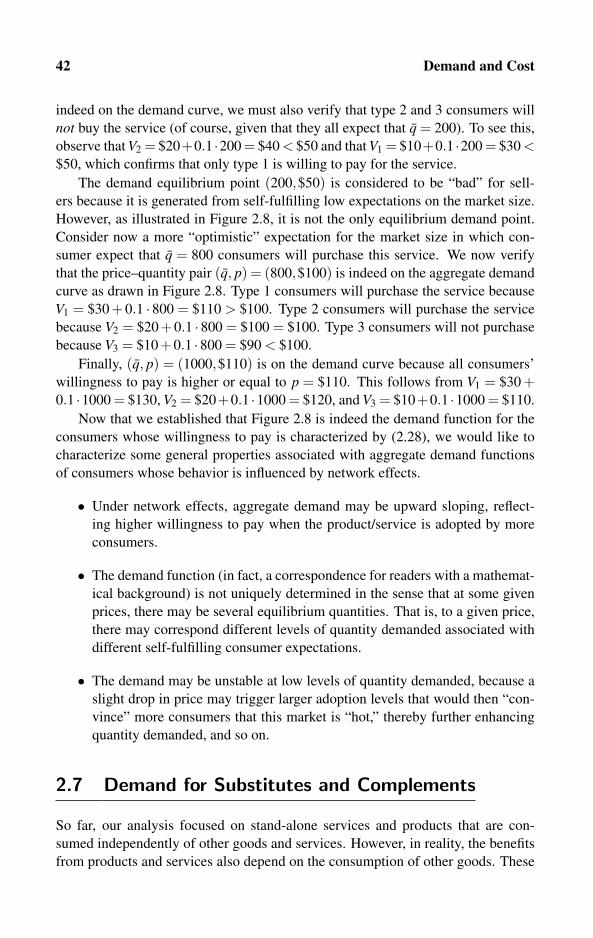
42 Demand and Cost
indeed on the demand curve, we must also verify that type 2 and 3 consumers will
not buy the service (of course, given that they all expect that q = 200). To see this,
observe that V2 = $20+0.1 ·200 = $40 < $50 and that V1 = $10+0.1 ·200 = $30 <$50, which confirms that only type 1 is willing to pay for the service.
The demand equilibrium point (200,$50) is considered to be “bad” for sell-
ers because it is generated from self-fulfilling low expectations on the market size.
However, as illustrated in Figure 2.8, it is not the only equilibrium demand point.
Consider now a more “optimistic” expectation for the market size in which con-
sumer expect that q = 800 consumers will purchase this service. We now verify
that the price–quantity pair (q, p) = (800,$100) is indeed on the aggregate demand
curve as drawn in Figure 2.8. Type 1 consumers will purchase the service because
V1 = $30 + 0.1 · 800 = $110 > $100. Type 2 consumers will purchase the service
because V2 = $20+0.1 ·800 = $100 = $100. Type 3 consumers will not purchase
because V3 = $10+0.1 ·800 = $90 < $100.
Finally, (q, p) = (1000,$110) is on the demand curve because all consumers’
willingness to pay is higher or equal to p = $110. This follows from V1 = $30 +0.1 ·1000 = $130, V2 = $20+0.1 ·1000 = $120, and V3 = $10+0.1 ·1000 = $110.
Now that we established that Figure 2.8 is indeed the demand function for the
consumers whose willingness to pay is characterized by (2.28), we would like to
characterize some general properties associated with aggregate demand functions
of consumers whose behavior is influenced by network effects.
• Under network effects, aggregate demand may be upward sloping, reflect-
ing higher willingness to pay when the product/service is adopted by more
consumers.
• The demand function (in fact, a correspondence for readers with a mathemat-
ical background) is not uniquely determined in the sense that at some given
prices, there may be several equilibrium quantities. That is, to a given price,
there may correspond different levels of quantity demanded associated with
different self-fulfilling consumer expectations.
• The demand may be unstable at low levels of quantity demanded, because a
slight drop in price may trigger larger adoption levels that would then “con-
vince” more consumers that this market is “hot,” thereby further enhancing
quantity demanded, and so on.
2.7 Demand for Substitutes and Complements
So far, our analysis focused on stand-alone services and products that are con-
sumed independently of other goods and services. However, in reality, the benefits
from products and services also depend on the consumption of other goods. These

2.7 Demand for Substitutes and Complements 43
“other” goods may be produced by the same seller, or by different competing sell-
ers. In this section we analyze the demand for such goods by looking at systems of
aggregate demand equations.
Let us suppose that consumers choose their consumption levels of two goods,
labeled A and B. The market aggregate direct linear demand functions for goods Aand B are given by
qA(pA, pB) def= αA−βA pA + γA pB, (2.29)
qB(pA, pB) def= αB + γB pA−βB pB.
Thus, the demand for each good also depends on the price of the other good (in fact,
on the prices of all other goods in a more general setup). The parameters βA, βB, γA,
and γB must be estimated from real-life data, as we demonstrate below. In general,
unless network effects are present, one should expect to find that the parameters
βA and βB (known as the own-price effect parameters) are strictly negative, thereby
reflecting downward-sloping demand curves.
The signs of the remaining two parameters, γA and γB, have the following inter-
pretations:
DEFINITION 2.4
Consumers are said to view goods A and B as
(a) Substitutes, if an increase in the price of B increases the demand for A, and an
increase in the price of A increases the demand for B. In the present example,
γA > 0 and γB > 0.
(b) Complements, if an increase in the price of B decreases the demand for A (and
B), and an increase in the price of A decreases the demand for A (and B). In the
present example, γA < 0 and γB < 0.
In fact, for some purposes (for example, see the analysis of peak-load pricing
under interdependent demand in Section 6.6) it is more useful to use a system of
inverse demand functions rather than a system of direct demand functions. Thus,
inverting the system of inverse demand (2.29) obtains the system of inverse demand
functions given by
pA(qA,qB) =αAβB +αBγA−βBqA− γAqB
βAβB− γAγB, (2.30)
pA(qA,qB) =αBβA +αAγB−βAqB− γBqA
βAβB− γAγB.
Clearly, it must be assumed (or verified if the demand is estimated from actual data)
that βAβB > γAγB, which means that price is more sensitive to changes in its own
purchased quantity than changes in the quantity purchased of the competing brand.
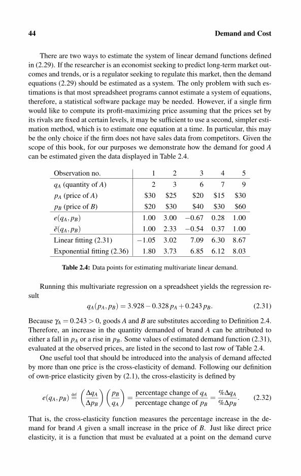
44 Demand and Cost
There are two ways to estimate the system of linear demand functions defined
in (2.29). If the researcher is an economist seeking to predict long-term market out-
comes and trends, or is a regulator seeking to regulate this market, then the demand
equations (2.29) should be estimated as a system. The only problem with such es-
timations is that most spreadsheet programs cannot estimate a system of equations,
therefore, a statistical software package may be needed. However, if a single firm
would like to compute its profit-maximizing price assuming that the prices set by
its rivals are fixed at certain levels, it may be sufficient to use a second, simpler esti-
mation method, which is to estimate one equation at a time. In particular, this may
be the only choice if the firm does not have sales data from competitors. Given the
scope of this book, for our purposes we demonstrate how the demand for good Acan be estimated given the data displayed in Table 2.4.
Observation no. 1 2 3 4 5
qA (quantity of A) 2 3 6 7 9
pA (price of A) $30 $25 $20 $15 $30
pB (price of B) $20 $30 $40 $30 $60
e(qA, pB) 1.00 3.00 −0.67 0.28 1.00
e(qA, pB) 1.00 2.33 −0.54 0.37 1.00
Linear fitting (2.31) −1.05 3.02 7.09 6.30 8.67
Exponential fitting (2.36) 1.80 3.73 6.85 6.12 8.03
Table 2.4: Data points for estimating multivariate linear demand.
Running this multivariate regression on a spreadsheet yields the regression re-
sult
qA(pA, pB) = 3.928−0.328 pA +0.243 pB. (2.31)
Because γA = 0.243 > 0, goods A and B are substitutes according to Definition 2.4.
Therefore, an increase in the quantity demanded of brand A can be attributed to
either a fall in pA or a rise in pB. Some values of estimated demand function (2.31),
evaluated at the observed prices, are listed in the second to last row of Table 2.4.
One useful tool that should be introduced into the analysis of demand affected
by more than one price is the cross-elasticity of demand. Following our definition
of own-price elasticity given by (2.1), the cross-elasticity is defined by
e(qA, pB) def=(
ΔqA
ΔpB
)(pB
qA
)=
percentage change of qA
percentage change of pB=
%ΔqA
%ΔpB. (2.32)
That is, the cross-elasticity function measures the percentage increase in the de-
mand for brand A given a small increase in the price of B. Just like direct price
elasticity, it is a function that must be evaluated at a point on the demand curve
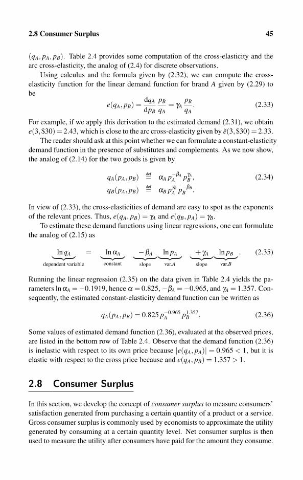
2.8 Consumer Surplus 45
(qA, pA, pB). Table 2.4 provides some computation of the cross-elasticity and the
arc cross-elasticity, the analog of (2.4) for discrete observations.
Using calculus and the formula given by (2.32), we can compute the cross-
elasticity function for the linear demand function for brand A given by (2.29) to
be
e(qA, pB) =dqA
dpB
pB
qA= γA
pB
qA. (2.33)
For example, if we apply this derivation to the estimated demand (2.31), we obtain
e(3,$30) = 2.43, which is close to the arc cross-elasticity given by e(3,$30) = 2.33.
The reader should ask at this point whether we can formulate a constant-elasticity
demand function in the presence of substitutes and complements. As we now show,
the analog of (2.14) for the two goods is given by
qA(pA, pB) def= αA p−βAA pγA
B , (2.34)
qB(pA, pB) def= αB pγBA p−βB
B .
In view of (2.33), the cross-elasticities of demand are easy to spot as the exponents
of the relevant prices. Thus, e(qA, pB) = γA and e(qB, pA) = γB.
To estimate these demand functions using linear regressions, one can formulate
the analog of (2.15) as
lnqA︸ ︷︷ ︸dependent variable
= lnαA︸ ︷︷ ︸constant
−βA︸ ︷︷ ︸slope
ln pA︸ ︷︷ ︸var.A
+ γA︸ ︷︷ ︸slope
ln pB︸ ︷︷ ︸var.B
. (2.35)
Running the linear regression (2.35) on the data given in Table 2.4 yields the pa-
rameters lnαA =−0.1919, hence α = 0.825,−βA =−0.965, and γA = 1.357. Con-
sequently, the estimated constant-elasticity demand function can be written as
qA(pA, pB) = 0.825 p−0.965A p1.357
B . (2.36)
Some values of estimated demand function (2.36), evaluated at the observed prices,
are listed in the bottom row of Table 2.4. Observe that the demand function (2.36)
is inelastic with respect to its own price because |e(qA, pA)| = 0.965 < 1, but it is
elastic with respect to the cross price because and e(qA, pB) = 1.357 > 1.
2.8 Consumer Surplus
In this section, we develop the concept of consumer surplus to measure consumers’
satisfaction generated from purchasing a certain quantity of a product or a service.
Gross consumer surplus is commonly used by economists to approximate the utility
generated by consuming at a certain quantity level. Net consumer surplus is then
used to measure the utility after consumers have paid for the amount they consume.
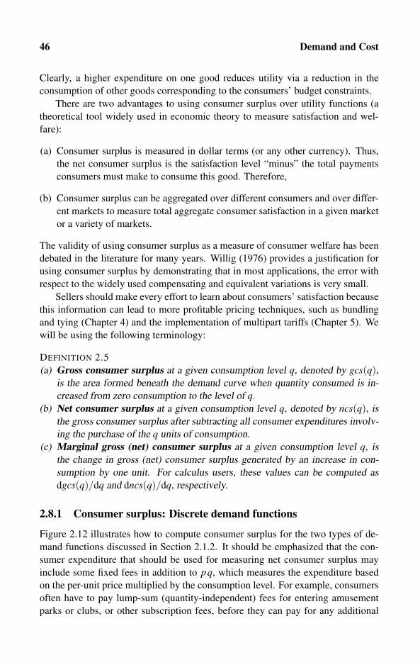
46 Demand and Cost
Clearly, a higher expenditure on one good reduces utility via a reduction in the
consumption of other goods corresponding to the consumers’ budget constraints.
There are two advantages to using consumer surplus over utility functions (a
theoretical tool widely used in economic theory to measure satisfaction and wel-
fare):
(a) Consumer surplus is measured in dollar terms (or any other currency). Thus,
the net consumer surplus is the satisfaction level “minus” the total payments
consumers must make to consume this good. Therefore,
(b) Consumer surplus can be aggregated over different consumers and over differ-
ent markets to measure total aggregate consumer satisfaction in a given market
or a variety of markets.
The validity of using consumer surplus as a measure of consumer welfare has been
debated in the literature for many years. Willig (1976) provides a justification for
using consumer surplus by demonstrating that in most applications, the error with
respect to the widely used compensating and equivalent variations is very small.
Sellers should make every effort to learn about consumers’ satisfaction because
this information can lead to more profitable pricing techniques, such as bundling
and tying (Chapter 4) and the implementation of multipart tariffs (Chapter 5). We
will be using the following terminology:
DEFINITION 2.5
(a) Gross consumer surplus at a given consumption level q, denoted by gcs(q),is the area formed beneath the demand curve when quantity consumed is in-
creased from zero consumption to the level of q.
(b) Net consumer surplus at a given consumption level q, denoted by ncs(q), is
the gross consumer surplus after subtracting all consumer expenditures involv-
ing the purchase of the q units of consumption.
(c) Marginal gross (net) consumer surplus at a given consumption level q, is
the change in gross (net) consumer surplus generated by an increase in con-
sumption by one unit. For calculus users, these values can be computed as
dgcs(q)/dq and dncs(q)/dq, respectively.
2.8.1 Consumer surplus: Discrete demand functions
Figure 2.12 illustrates how to compute consumer surplus for the two types of de-
mand functions discussed in Section 2.1.2. It should be emphasized that the con-
sumer expenditure that should be used for measuring net consumer surplus may
include some fixed fees in addition to pq, which measures the expenditure based
on the per-unit price multiplied by the consumption level. For example, consumers
often have to pay lump-sum (quantity-independent) fees for entering amusement
parks or clubs, or other subscription fees, before they can pay for any additional
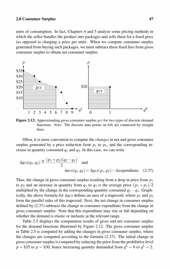
2.8 Consumer Surplus 47
units of consumption. In fact, Chapters 4 and 5 analyze some pricing methods in
which the seller bundles the product into packages and sells them for a fixed price
(as opposed to charging a price per unit). When we compute consumer surplus
generated from buying such packages, we must subtract these fixed fees from gross
consumer surplus to obtain net consumer surplus.
� �
� �
qRqL
pp
•$30
$25
••
$20
$15
$10
2 6 7 93 4 5 81 1
$20
0
•
••
•
$35•
gcsgcs
Figure 2.12: Approximating gross consumer surplus gcs for two types of discrete demand
functions. Note: The discrete data points on left are connected by straight
lines.
Often, it is more convenient to compute the changes in net and gross consumer
surplus generated by a price reduction from p1 to p2, and the corresponding in-
crease in quantity consumed q1 and q2. In this case, we can write
Δgcs(q1,q2)def=
(p1 + p2)(q2−q1)2
and
Δncs(q1,q2) = Δgcs(p1, p2)−Δexpenditure. (2.37)
Thus, the change in gross consumer surplus resulting from a drop in price from p1
to p2 and an increase in quantity from q1 to q2 is the average price (p1 + p2)/2
multiplied by the change in the corresponding quantity consumed q2−q1. Graph-
ically, the above formula for Δgcs defines an area of a trapezoid, where p1 and p2
form the parallel sides of this trapezoid. Next, the net change in consumer surplus
defined by (2.37) subtracts the change in consumer expenditure from the change in
gross consumer surplus. Note that this expenditure may rise or fall depending on
whether the demand is elastic or inelastic at the relevant range.
Table 2.5 displays the computation results of gross and net consumer surplus
for the demand functions illustrated by Figure 2.12. The gross consumer surplus
in Table 2.5 is computed by adding the changes in gross consumer surplus, where
the changes are computed according to the formula (2.37). The initial change in
gross consumer surplus is computed by reducing the price from the prohibitive level
p = $35 to p = $30, hence increasing quantity demanded from qL = 0 to qL = 2.
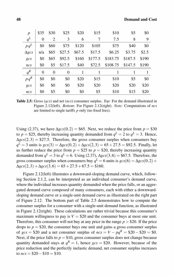
48 Demand and Cost
p $35 $30 $25 $20 $15 $10 $5 $0
qL 0 2 3 6 7 7.5 8 9
pqL $0 $60 $75 $120 $105 $75 $40 $0
Δgcs n/a $65 $27.5 $67.5 $17.5 $6.25 $3.75 $2.5
gcs $0 $65 $92.5 $160 $177.5 $183.75 $187.5 $190
ncs $0 $5 $17.5 $40 $72.5 $108.75 $147.5 $190
qR 0 0 0 1 1 1 1 1
pqR $0 $0 $0 $20 $15 $10 $5 $0
gcs $0 $0 $0 $20 $20 $20 $20 $20
ncs $0 $5 $0 $0 $5 $10 $15 $20
Table 2.5: Gross (gcs) and net (ncs) consumer surplus. Top: For the demand illustrated in
Figure 2.12(left). Bottom: For Figure 2.12(right). Note: Computations of ncsare limited to single tariffs p only (no fixed fees).
Using (2.37), we have Δgcs(0,2) = $65. Next, we reduce the price from p = $30
to p = $25, thereby increasing quantity demanded from qL = 2 to qL = 3. Hence,
Δgcs(2,3) = $27.5. Therefore, the gross consumer surplus when consumers buy
qL = 3 units is gcs(3) = Δgcs(0,2)+ Δgcs(2,3) = 65 + 27.5 = $92.5. Finally, let
us further reduce the price from p = $25 to p = $20, thereby increasing quantity
demanded from qL = 3 to qL = 6. Using (2.37), Δgcs(3,6) = $67.5. Therefore, the
gross consumer surplus when consumers buy qL = 6 units is gcs(6) = Δgcs(0,2)+Δgcs(2,3)+Δgcs(3,6) = 65+27.5+67.5 = $160.
Figure 2.12(left) illustrates a downward-sloping demand curve, which, follow-
ing Section 2.1.2, can be interpreted as an individual consumer’s demand curve,
where the individual increases quantity demanded when the price falls, or an aggre-
gated demand curve composed of many consumers, each with either a downward-
sloping demand curve or a single-unit demand curve as illustrated on the right part
of Figure 2.12. The bottom part of Table 2.5 demonstrates how to compute the
consumer surplus for a consumer with a single-unit demand function, as illustrated
in Figure 2.12(right). These calculations are rather trivial because this consumer’s
maximum willingness to pay is V = $20 and the consumer buys at most one unit.
Therefore, this consumer will not buy at any price in the range p > $20. If the price
drops to p = $20, the consumer buys one unit and gains a gross consumer surplus
of gcs = $20 and a net consumer surplus of ncs = V − pqR = $20− $20 = $0.
Next, if the price falls to p = $10, gross consumer surplus does not change because
quantity demanded stays at qR = 1, hence gcs = $20. However, because of the
price reduction and the perfectly inelastic demand, net consumer surplus increases
to ncs = $20−$10 = $10.

2.8 Consumer Surplus 49
q[1]← 0; gcs[1]← 0; /* High p[1] generates zero demand */for � = 2 to M do
/* Loop over demand observations and Price reductions */Δgcs[�]← (p[�−1]+ p[�])(q[�]−q[�−1])/2; /* Change in gcs */gcs[�]← gcs[�−1]+Δgcs[�]; /* gcs at q[�] units */writeln (“At the price p =”, p[�], “quantity demanded is q = ”, q[�],“gross consumer surplus is gcs =”, gcs[�]);writeln (“Increasing consumption from ”, q[�−1], “to ”, q[�], has
increased gross consumer surplus by ”, Δgcs[�]);
Algorithm 2.3: Computing gross consumer surplus for discrete demand.
Algorithm 2.3 computes gross consumer surplus for discrete demand func-
tions. Algorithm 2.3 should input, using the Read() command, and store the data
points of the discrete demand function based on M ≥ 1 price–quantity observa-
tions. More precisely, the program must input the price p[�] and the corresponding
quantity demanded q[�] for each observation � = 1, . . . ,M, where p[�] and q[�] are
M-dimensional arrays of real-valued demand observations. It is recommended that
the program run some trivial loops verifying nonnegativity as well as some strictly
positive demand observation. It is very important that prices be ordered from high
to low so that p[1] > p[2] > · · · > p[M] and that p[1] will be sufficiently high to
induce q[1] = 0 (zero consumption). In any case, the proposed algorithm assigns
q[1]← 0 as otherwise consumer surplus cannot be computed for discrete demand.
Algorithm 2.3 runs a loop over all observations � = 2, · · · ,M, and computes
the change in gross consumer surplus. Then, it adds up this change to the gross
consumer surplus computed for previous observation. Thus, the program outputs
the results onto the real-valued M-dimensional arrays Δgcs[�] and gcs[�], where the
algorithm presets gcs[1]← 0 and q[1]← 0 (no consumption).
2.8.2 Consumer surplus: Continuous demand functions
The computations of gross consumer surplus turn out to be much simpler when
applied to continuous linear and constant-elasticity demand functions. The left
part of Figure 2.13 illustrates how to compute gross consumer surplus for the linear
demand function analyzed in Section 2.3. Figure 2.13(right) illustrates how to com-
pute gross consumer surplus for the constant-elasticity demand function analyzed
in Section 2.4.

50 Demand and Cost
� �
� �
pp
$30
$25
$20
$15
$10
20 60 7030 40 50 8010
$35����������
gcs
= 35− 12q
p = α−βq
gcs
p =( q
α)− 1
β
Figure 2.13: Gross consumer surplus. Left: Linear demand function. Right: Constant-
elasticity demand function.
Linear demand function
Figure 2.13(left) is drawn according to p = 35− 0.5q. For this particular linear
demand function, the gross consumer surplus evaluated at a consumption level of
q = 40 units is the area of the trapezoid defined by
gcs(40) =(35+15)(40−0)
2= $1000. (2.38)
For the general linear demand case p = α−βq, the gross consumer surplus at any
arbitrary consumption level q is
gcs(q) =(α + p)(q−0)
2=
(α +α−βq)(q−0)2
=(2α−βq)q
2. (2.39)
Readers who prefer to use calculus can simply integrate the inverse demand func-
tion∫ q
0 (α −βq)dq to obtain (2.39). In fact, the formula derived in (2.39) can be
extended to capture the change in consumer surplus generated by increasing con-
sumption from q1 to q2 so that
Δgcs(q1,q2) =(p1 + p2)(q2−q1)
2=
(α−βq1 +α−βq2)(q2−q1)2
=(q2−q1)[2α−β (q1 +q2)]
2. (2.40)
If we return to the specific example drawn in Figure 2.13(left) where p = 35−0.5q,
formula (2.40) implies that the change in consumer surplus generated by increasing
consumption from q1 = 20 to q2 = 40 is Δgcs(20,40) = $400.
Several chapters in this book make heavy use of the consumer surplus concept.
For example, a proper characterization of consumer surplus is essential for pricing
bundles of products and services containing more than one unit of consumption

2.8 Consumer Surplus 51
(see Chapter 4). Therefore, it is often useful to plot consumer surplus as a function
of quantity consumed. Figure 2.14 illustrates the gross consumer surplus (2.39)
derived from the general demand function p = α−βq (also plotted).
�
αβ
α
α2
2β
p, gcs
p(q) = α−βq
gcs(q) = 12(2α−βq)q
� q
Figure 2.14: Illustration of gross consumer surplus for linear demand. Note: Figure is not
drawn to scale.
Calculus lovers who wish to characterize the gross consumer surplus function
can simply differentiate (2.39) with respect to quantity consumed to obtain
dgcs(q)dq
= α−βq = p(q). (2.41)
That is, the marginal gross consumer surplus function (see Definition 2.5(c)) is
equal to the inverse demand function that equals the price a consumer is willing to
pay at a given consumption level. Intuitively, the change in gross consumer surplus
associated with a small increase in consumption (the marginal gross consumer sur-
plus) must be equal to the consumer’s willingness to pay as captured by the price
on the inverse demand function.
Constant-elasticity demand function
Figure 2.13(right) illustrates the inverse demand function derived from the direct
constant-elasticity demand function q = α(q)−β , which was analyzed in Section 2.4.
Thus, assuming β > 1 (elastic demand), the inverse demand function and the cor-
responding gross consumer surplus are given by
p =( q
α
)− 1β
hence gcs(q) =q∫
0
( xα
)− 1β
dx =βq( q
α)− 1
β
β −1. (2.42)
The gross consumer surplus (2.42) evaluated at a given consumption level q is
marked by the shaded area in Figure 2.13(right).
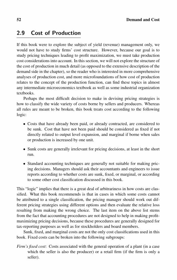
52 Demand and Cost
2.9 Cost of Production
If this book were to explore the subject of yield (revenue) management only, we
would not have to study firms’ cost structure. However, because our goal is to
study pricing techniques leading to profit maximization, we must take production
cost considerations into account. In this section, we will not explore the structure of
the cost of production in much detail (as opposed to the extensive description of the
demand side in the chapter), so the reader who is interested in more comprehensive
analyses of production cost, and more microfoundations of how cost of production
relates to the concept of the production function, can find these topics in almost
any intermediate microeconomics textbook as well as some industrial organization
textbooks.
Perhaps the most difficult decision to make in devising pricing strategies is
how to classify the wide variety of costs borne by sellers and producers. Whereas
all rules are meant to be broken, this book treats cost according to the following
logic:
• Costs that have already been paid, or already contracted, are considered to
be sunk. Cost that have not been paid should be considered as fixed if not
directly related to output level expansion, and marginal if borne when sales
or production is increased by one unit.
• Sunk costs are generally irrelevant for pricing decisions, at least in the short
run.
• Standard accounting techniques are generally not suitable for making pric-
ing decisions. Managers should ask their accountants and engineers to issue
reports according to whether costs are sunk, fixed, or marginal, or according
to some other cost classification discussed in this book.
This “logic” implies that there is a great deal of arbitrariness in how costs are clas-
sified. What this book recommends is that in cases in which some costs cannot
be attributed to a single classification, the pricing manager should work out dif-
ferent pricing strategies using different options and then evaluate the relative loss
resulting from making the wrong choice. The last item on the above list stems
from the fact that accounting procedures are not designed to help in making profit-
maximizing pricing decisions, because these procedures are generally designed for
tax-reporting purposes as well as for stockholders and board members.
Sunk, fixed, and marginal costs are not the only cost classifications used in this
book. Fixed costs can be broken into the following subgroups:
Firm’s fixed cost: Costs associated with the general operation of a plant (in a case
which the seller is also the producer) or a retail firm (if the firm is only a
seller).

2.9 Cost of Production 53
Market specific: Costs associated with entry and maintaining a presence in differ-
ent markets.
Clearly, entry fixed costs become sunk after entry is completed and fixed costs are
reduced to the general cost of operating in the specific market. The firm’s total
fixed cost is denoted by φ , and market � fixed cost is denoted by φ� for each market
� = 1, . . . ,M.
Marginal costs can be broken into the following two subgroups:
Marginal operating cost: Cost associated with serving one additional customer.
Marginal capacity cost: Cost of increasing capacity that enables the production of
one additional unit, or serves one additional consumer.
For example, the marginal operating cost for an electricity company is the addi-
tional fuel and transmission costs associated with the production and sale of one
additional kilowatt per hour. The marginal capacity cost would be the cost of up-
grading production and transmission capacity to generate one additional kilowatt
per hour. This distinction becomes important in Chapter 6, where we analyze peak
and off-peak pricing, as well as in Chapters 7 and 8, where we analyze airline
booking strategies.
From a technical point of view, in what follows we focus our analysis on cost
structures confined to constant marginal cost only. Perhaps the simplest represen-
tation of a firm’s cost structure is given by
c(q) =
{φ + μ q if q > 0
0 if q = 0,(2.43)
where q≥ 0 is the output level of the firm. The parameter φ is called a fixed or sunkcost that sums up all the firm’s costs that are independent of the chosen output level.
Formula (2.43) assumes that the firm has the option of going out of service, thereby
avoiding paying the fixed cost φ . However, as long as some output is produced, the
firm must bear the full amount.
The parameter μ is called the marginal cost of production and is defined as the
change in cost associated with an increase in output by one unit (or infinitesimal
change if calculus is used). Formally, for nonnegative output levels q≥ 0, we define
the marginal and average cost functions by
Δc(q)Δq
= μ andc(q)
q=
φq
+ μ. (2.44)
Unlike the marginal cost, which measures the change in cost when output level
slightly increases from a certain level q, the average cost measures the production
cost per unit of output. Inspecting (2.44) reveals that under the present specification
(where the marginal cost μ is constant), the average cost would be equal to the
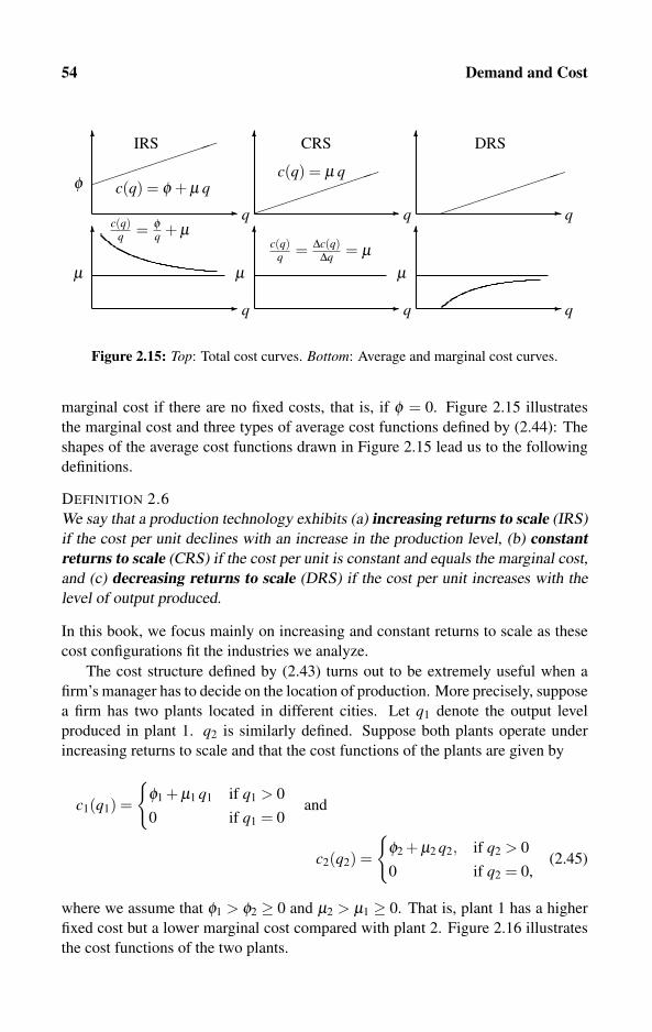
54 Demand and Cost
�
� q
�
� q
�
� q
�
� q
�
� q
�
� q
φ
μ
c(q) = φ + μ q
c(q)q = φ
q + μ
μ μ
c(q) = μ q
c(q)q = Δc(q)
Δq = μ
IRS CRS DRS
Figure 2.15: Top: Total cost curves. Bottom: Average and marginal cost curves.
marginal cost if there are no fixed costs, that is, if φ = 0. Figure 2.15 illustrates
the marginal cost and three types of average cost functions defined by (2.44): The
shapes of the average cost functions drawn in Figure 2.15 lead us to the following
definitions.
DEFINITION 2.6
We say that a production technology exhibits (a) increasing returns to scale (IRS)
if the cost per unit declines with an increase in the production level, (b) constantreturns to scale (CRS) if the cost per unit is constant and equals the marginal cost,
and (c) decreasing returns to scale (DRS) if the cost per unit increases with the
level of output produced.
In this book, we focus mainly on increasing and constant returns to scale as these
cost configurations fit the industries we analyze.
The cost structure defined by (2.43) turns out to be extremely useful when a
firm’s manager has to decide on the location of production. More precisely, suppose
a firm has two plants located in different cities. Let q1 denote the output level
produced in plant 1. q2 is similarly defined. Suppose both plants operate under
increasing returns to scale and that the cost functions of the plants are given by
c1(q1) =
{φ1 + μ1 q1 if q1 > 0
0 if q1 = 0and
c2(q2) =
{φ2 + μ2 q2, if q2 > 0
0 if q2 = 0,(2.45)
where we assume that φ1 > φ2 ≥ 0 and μ2 > μ1 ≥ 0. That is, plant 1 has a higher
fixed cost but a lower marginal cost compared with plant 2. Figure 2.16 illustrates
the cost functions of the two plants.
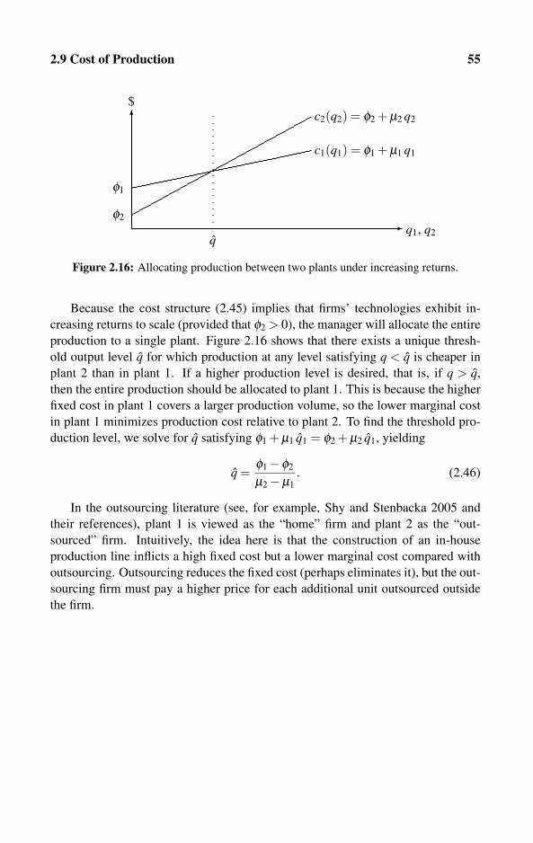
2.9 Cost of Production 55
� c2(q2) = φ2 + μ2 q2
� q1, q2
$
q
φ2
φ1
c1(q1) = φ1 + μ1 q1
Figure 2.16: Allocating production between two plants under increasing returns.
Because the cost structure (2.45) implies that firms’ technologies exhibit in-
creasing returns to scale (provided that φ2 > 0), the manager will allocate the entire
production to a single plant. Figure 2.16 shows that there exists a unique thresh-
old output level q for which production at any level satisfying q < q is cheaper in
plant 2 than in plant 1. If a higher production level is desired, that is, if q > q,
then the entire production should be allocated to plant 1. This is because the higher
fixed cost in plant 1 covers a larger production volume, so the lower marginal cost
in plant 1 minimizes production cost relative to plant 2. To find the threshold pro-
duction level, we solve for q satisfying φ1 + μ1 q1 = φ2 + μ2 q1, yielding
q =φ1−φ2
μ2−μ1. (2.46)
In the outsourcing literature (see, for example, Shy and Stenbacka 2005 and
their references), plant 1 is viewed as the “home” firm and plant 2 as the “out-
sourced” firm. Intuitively, the idea here is that the construction of an in-house
production line inflicts a high fixed cost but a lower marginal cost compared with
outsourcing. Outsourcing reduces the fixed cost (perhaps eliminates it), but the out-
sourcing firm must pay a higher price for each additional unit outsourced outside
the firm.

56 Demand and Cost
2.10 Exercises
1. Fill in the missing parts in Table 2.6 based on the discrete demand analysis in
Section 2.2.
p $9.5 $9.0 $8.5 $8.0 $7.5 $7.0 $6.5 $6.0
q 15 16 17 18 19 20 21 22
e(q)e(q)x(q)Δx(q)
Δq
Table 2.6: Data for Exercises 1 and 2.
.
2. Use a computer to estimate linear and constant-elasticity demand using the raw
data on demand observations given in the first two lines of Table 2.6.
(a) Using the procedure described in Section 2.3.2, estimate the parameters γand δ of the direct linear demand function p(q) = γ−δq.
(b) Formulate the inverse demand function corresponding to the direct demand
function you estimated in part (a).
(c) Using the procedure described in Section 2.4.2, estimate the parameters αand β of the direct constant-elasticity demand function q(p) = α p−β .
(d) What is the value of the elasticity of the constant-elasticity demand function
you have estimated? Is this function elastic or inelastic?
3. Consider the following direct linear demand function q(p) = 34−2p.
(a) Formulate the corresponding inverse demand function p(q) and the revenue
function x(q).
(b) This exercise requires the use of calculus. Using the analysis of Section 2.3.3,
compute the revenue maximizing output level and the corresponding price.
(c) Compute the resulting revenue level and the price elasticity assuming that a
single firm sells the revenue-maximizing output level.
4. Consider the example of aggregating single-unit demand functions analyzed in
Section 2.5.1 and plotted in Figure 2.8. Suppose that a fourth type of new con-
sumers N4 = 200 enters this market (say, because of a large wave of immigration
into this city). Draw the new aggregate demand function assuming that the max-
imum willingness to pay of each newly entering consumer is $25.
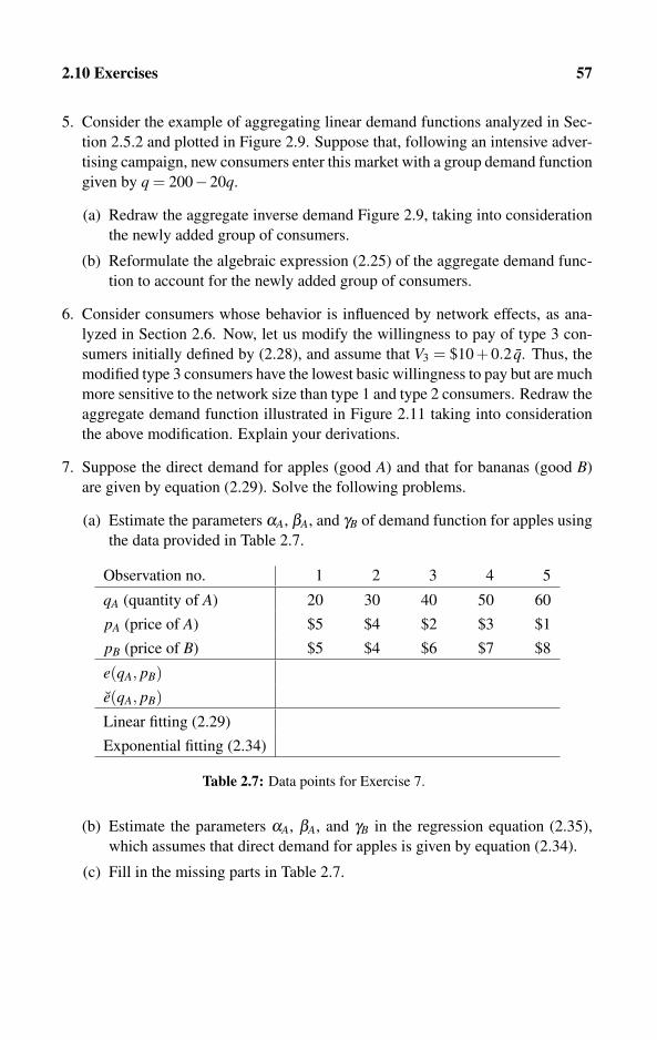
2.10 Exercises 57
5. Consider the example of aggregating linear demand functions analyzed in Sec-
tion 2.5.2 and plotted in Figure 2.9. Suppose that, following an intensive adver-
tising campaign, new consumers enter this market with a group demand function
given by q = 200−20q.
(a) Redraw the aggregate inverse demand Figure 2.9, taking into consideration
the newly added group of consumers.
(b) Reformulate the algebraic expression (2.25) of the aggregate demand func-
tion to account for the newly added group of consumers.
6. Consider consumers whose behavior is influenced by network effects, as ana-
lyzed in Section 2.6. Now, let us modify the willingness to pay of type 3 con-
sumers initially defined by (2.28), and assume that V3 = $10 + 0.2 q. Thus, the
modified type 3 consumers have the lowest basic willingness to pay but are much
more sensitive to the network size than type 1 and type 2 consumers. Redraw the
aggregate demand function illustrated in Figure 2.11 taking into consideration
the above modification. Explain your derivations.
7. Suppose the direct demand for apples (good A) and that for bananas (good B)
are given by equation (2.29). Solve the following problems.
(a) Estimate the parameters αA, βA, and γB of demand function for apples using
the data provided in Table 2.7.
Observation no. 1 2 3 4 5
qA (quantity of A) 20 30 40 50 60
pA (price of A) $5 $4 $2 $3 $1
pB (price of B) $5 $4 $6 $7 $8
e(qA, pB)e(qA, pB)
Linear fitting (2.29)
Exponential fitting (2.34)
Table 2.7: Data points for Exercise 7.
(b) Estimate the parameters αA, βA, and γB in the regression equation (2.35),
which assumes that direct demand for apples is given by equation (2.34).
(c) Fill in the missing parts in Table 2.7.
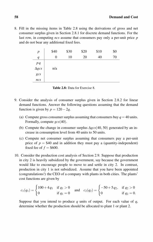
58 Demand and Cost
8. Fill in the missing items in Table 2.8 using the derivations of gross and net
consumer surplus given in Section 2.8.1 for discrete demand functions. For the
last row, in computing ncs assume that consumers pay only a per-unit price pand do not bear any additional fixed fees.
p $40 $30 $20 $10 $0
q 0 10 20 40 70
pq
Δgcs n/a
gcs
ncs
Table 2.8: Data for Exercise 8.
9. Consider the analysis of consumer surplus given in Section 2.8.2 for linear
demand functions. Answer the following questions assuming that the demand
function is given by p = 120−2q.
(a) Compute gross consumer surplus assuming that consumers buy q = 40 units.
Formally, compute gcs(40).
(b) Compute the change in consumer surplus Δgcs(40, 50) generated by an in-
crease in consumption level from 40 units to 50 units.
(c) Compute net consumer surplus assuming that consumers pay a per-unit
price of p = $40 and in addition they must pay a (quantity-independent)
fixed fee of f = $600.
10. Consider the production cost analysis of Section 2.9. Suppose that production
in city 2 is heavily subsidized by the government, say because the government
would like to encourage people to move to and settle in city 2. In contrast,
production in city 1 is not subsidized. Assume that you have been appointed
(congratulations!) the CEO of a company with plants in both cities. The plants’
cost functions are given by
c1(q1) =
{100+4q1 if q1 > 0
0 if q1 = 0and c2(q2) =
{−50+5q2, if q2 > 0
0 if q2 = 0.
Suppose that you intend to produce q units of output. For each value of q,
determine whether the production should be allocated to plant 1 or plant 2.

Chapter 3
Basic Pricing Techniques
3.1 Single-market Pricing 603.1.1 Price setting under discrete demand
3.1.2 Quantity setting under continuous linear demand
3.1.3 Price setting under continuous linear demand
3.1.4 Continuous constant-elasticity demand
3.2 Multiple Markets without Price Discrimination 673.2.1 Market-specific fixed costs and exclusion of markets
3.2.2 A computer algorithm for market selections
3.2.3 Multiple markets under single-unit demand
3.2.4 Linear demand: Example for two markets
3.2.5 Linear demand: General formulation for two markets
3.2.6 Linear demand: A computer algorithm for multiple markets
3.3 Multiple Markets with Price Discrimination 793.3.1 Unlimited capacity: Linear demand
3.3.2 Unlimited capacity: Constant-elasticity demand
3.3.3 Price discrimination under capacity constraint
3.4 Pricing under Competition 893.4.1 Switching costs among homogeneous goods
3.4.2 Switching costs among differentiated brands
3.4.3 Continuous demand with differentiated brands
3.5 Commonly Practiced Pricing Methods 993.5.1 Breakeven formulas
3.5.2 Cost-plus pricing methods
3.6 Regulated Public Utility 1043.6.1 Allocating fixed costs across markets while breaking even
3.6.2 Allocating fixed costs: Ramsey pricing
3.7 Exercises 110
60 Basic Pricing Techniques
This chapter introduces basic pricing techniques. By basic we refer to techniques
that are limited to simple one-time purchases of a single good only. That is, the
simple techniques studied in this chapter do not address more sophisticated mar-
kets in which products and services are differentiated by the time of delivery, the
length of the booking period, quantity discounts (bundling), and services that are
tied with other products and services. In fact, some of basic pricing techniques
described in this chapter can also be found in most intermediate college micro-
economics textbooks. Clearly, readers must first understand these basic techniques
before proceeding to more sophisticated ones analyzed in later chapters.
The basic question that must be addressed before managers select a price is
whether competition with other firms prevails, or whether the firm can disregard
any potential and existing competition and act as a single-seller monopoly. Most of
the algorithms in this book are designed for a single seller simply because the intro-
duction of competition diverts attention from learning the logic behind proper yield
management. Clearly, prices should be lowered when a firm observes competition
from rival firms. In view of this discussion, we divide this chapter into the analysis
of basic monopoly pricing and only then proceed to analyze pricing under compe-
tition. The analysis of competition will be brief because there is a large number of
market structures that must be considered. The study of market structures defines a
subfield of economics called industrial organization and is found in most industrial
organization textbooks. A comprehensive analysis of market structure is therefore
beyond the scope of this book.
3.1 Single-market Pricing
Suppose that the seller is unable to segment the market into submarkets in which
each market serves a different group of consumers. In this case, all the consumers
are treated as a single market for which the seller must determine a single price.
Recalling our notation given in Tables 1.4 and 1.5, the parameter μ denotes the
seller’s marginal production cost and φ the fixed/sunk cost (see Section 2.9 for
precise definitions). The variable p denotes the price to be decided by the seller,
and q the associated quantity demanded.
Similar to our analysis in Chapter 2, we divide our examination into discrete
and continuous demand functions. A discrete demand analysis is generally more
suitable for computer computations. However, using discrete demand may be less
intuitive and harder to compute algebraically compared with the continuous de-
mand analysis. Clearly, the two types of demand functions are related, because
Sections 2.3.2 and 2.4.2 have already studied the techniques under which continu-
ous demand functions can be used to approximate discrete demand functions.
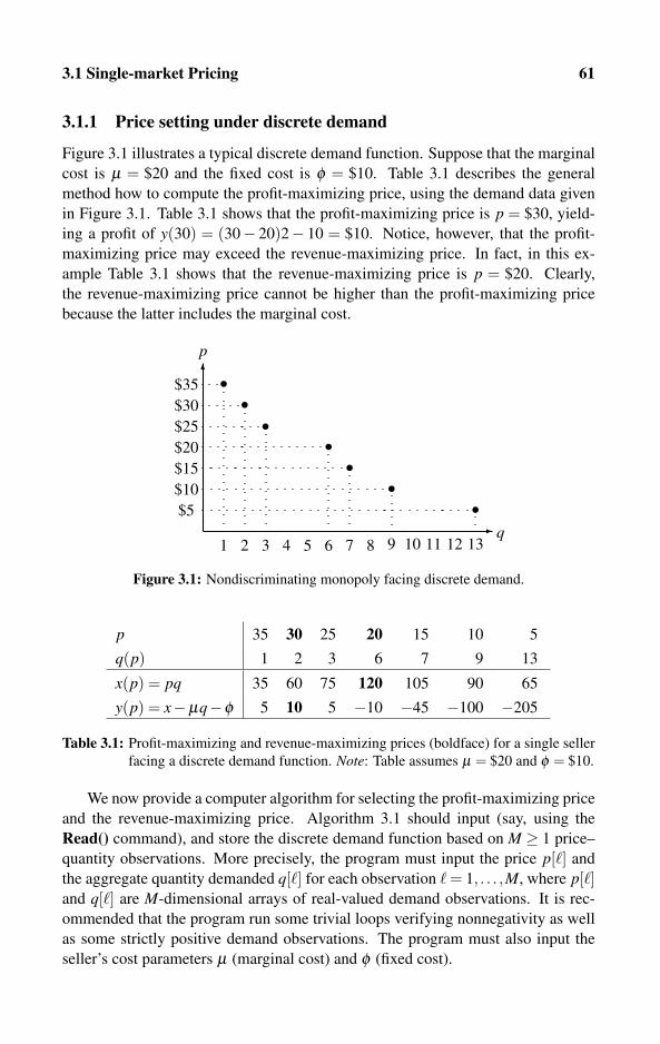
3.1 Single-market Pricing 61
3.1.1 Price setting under discrete demand
Figure 3.1 illustrates a typical discrete demand function. Suppose that the marginal
cost is μ = $20 and the fixed cost is φ = $10. Table 3.1 describes the general
method how to compute the profit-maximizing price, using the demand data given
in Figure 3.1. Table 3.1 shows that the profit-maximizing price is p = $30, yield-
ing a profit of y(30) = (30− 20)2− 10 = $10. Notice, however, that the profit-
maximizing price may exceed the revenue-maximizing price. In fact, in this ex-
ample Table 3.1 shows that the revenue-maximizing price is p = $20. Clearly,
the revenue-maximizing price cannot be higher than the profit-maximizing price
because the latter includes the marginal cost.
�
p
••$30
$25
••
•
$20
$15
$10
2 6 73 4 5 81 109 11 12�
13
$35
q•$5
•
Figure 3.1: Nondiscriminating monopoly facing discrete demand.
p 35 30 25 20 15 10 5
q(p) 1 2 3 6 7 9 13
x(p) = pq 35 60 75 120 105 90 65
y(p) = x−μq−φ 5 10 5 −10 −45 −100 −205
Table 3.1: Profit-maximizing and revenue-maximizing prices (boldface) for a single seller
facing a discrete demand function. Note: Table assumes μ = $20 and φ = $10.
We now provide a computer algorithm for selecting the profit-maximizing price
and the revenue-maximizing price. Algorithm 3.1 should input (say, using the
Read() command), and store the discrete demand function based on M ≥ 1 price–
quantity observations. More precisely, the program must input the price p[�] and
the aggregate quantity demanded q[�] for each observation � = 1, . . . ,M, where p[�]and q[�] are M-dimensional arrays of real-valued demand observations. It is rec-
ommended that the program run some trivial loops verifying nonnegativity as well
as some strictly positive demand observations. The program must also input the
seller’s cost parameters μ (marginal cost) and φ (fixed cost).

62 Basic Pricing Techniques
maxy← 0; maxx← 0; /* Initialization */for � = 1 to M do
/* Main loop over demand observations */if (p[�]−μ)q[�]−φ ≥maxy then
/* Higher profit found */maxy← (p[�]−μ)q[�]−φ ; maxpy← p[�];
if p[�]q[�]≥maxx thenmaxx← p[�]q[�]; maxpx← p[�]; /* Higher revenue found */
writeln (“The revenue-maximizing price is p =”, maxpx, “yielding the
revenue level x = ”, maxx);
if maxy≥ 0 thenwriteln (“The profit-maximizing price is p =”, maxpy, “yielding the
profit level y = ”, maxy);
else writeln (“Negative profit. Do NOT operate in this market!”)
Algorithm 3.1: Computing a monopoly’s profit- and revenue-maximizing
prices under discrete demand.
Algorithm 3.1 is rather straightforward. It runs a loop on all observations
� = 1,2, · · · ,M, and computes the profit and revenue levels. Each loop also checks
whether the computed levels exceed currently maximized levels stored in nonneg-
ative real variables denoted by maxpy (profit-maximizing price), maxpx (revenue-
maximizing price), maxy (maximum profit), and maxx (maximum revenue).
Finally, Algorithm 3.1 could be enhanced to compute what some textbooks call
the short-run profit. Short-run profit is generally defined as the profit level assuming
zero fixed cost. That is, (p−μ)q. In the above algorithm, the maximum short-run
profit is simply maxy + φ . If this value is nonnegative, the seller may want to
consider the option of staying in business until the fixed cost must be repaid, and
only then get out of business (delayed bankruptcy).
3.1.2 Quantity setting under continuous linear demand
One advantage of using a continuous demand function is that it makes it easy to
obtain the profit-maximizing quantity produced and the corresponding price us-
ing simple algebraic computations (as opposed to having to run loops over all the
observed price–quantity combinations, for the case of discrete demand functions).
Section 2.3.2 has already demonstrated how a linear function can be used to ap-
proximate scattered price and quantity observations.
We now refer the reader back to Section 2.3, where equation (2.6) defines the
inverse linear demand function given by p(q) = α − βq, where the parameters
α,β > 0 are to be estimated by the econometrician. Recalling equations (2.11)

3.1 Single-market Pricing 63
and (2.12), the total and marginal revenue functions are given by
x(q) = p(q)q = αq−βq2 anddx(q)
dq=
d[p(q)q]dq
= α−2βq. (3.1)
Let μ denote the marginal production/selling cost, and φ the fixed cost. The
seller must first verify that the intercept of the inverse demand function exceeds
the marginal cost, that is, α > μ . Otherwise, consumers’ willingness to pay is
below the marginal cost, which means that this product is not profitable even if the
fixed cost is not taken into account. We are now ready to describe the procedure
for selecting the monopoly’s profit-maximizing price assuming that α > μ . As it
turns out, it is much simpler to search for the monopoly’s profit-maximizing output
level first, and only then, using the inverse demand function, determine the profit-
maximizing price. The following procedure uses this approach.
Step I: Increase quantity produced until the revenue generated from selling the last
unit (the marginal revenue) equals marginal cost. Formally, use (3.1) to solve
dx(q)dq
= μ to obtain q =α−μ
2β. (3.2)
Step II: Compute the “candidate” profit-maximizing price by substituting into the
inverse demand function
p = α−βq to obtain p =α + μ
2. (3.3)
Step III: Compute the profit level y by solving
y = (p−μ)q−φ to obtain y =(α−μ)2
4β−φ . (3.4)
If y≥ 0, then p given in (3.3) is the profit-maximizing price. Otherwise, the
firm should not sell anything as this market is not profitable.
Note again that even if (3.4) is negative (the seller is making a loss), the seller may
want to consider the option of staying in business until the fixed cost has to be
repaid, and only then get out of business (delayed bankruptcy).
Figure 3.2 provides a visual interpretation for the above three-step procedure.
The “candidate” profit-maximizing output is determined by the intersection of the
marginal revenue function with the marginal cost function (lower thick dot). Then,
from this point, extending the line upward toward the demand line yields the profit-
maximizing price (upper thick dot) because consumers are always on their demand
curve. However, note that all these are necessary conditions for profit maximiza-
tion, which are not sufficient. For this reason, to complete this procedure, Step III
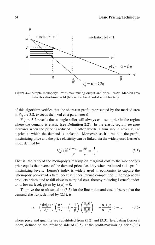
64 Basic Pricing Techniques
�
�
q
α
α2β
elastic: |e|> 1
p
p(q) = α−β q
ΔxΔq = α−2βq
αβ
μ
p
q
μ •
•
inelastic: |e|< 1
Figure 3.2: Simple monopoly: Profit-maximizing output and price. Note: Marked area
indicates short-run profit (before the fixed cost φ is subtracted).
of this algorithm verifies that the short-run profit, represented by the marked area
in Figure 3.2, exceeds the fixed cost parameter φ .
Figure 3.2 reveals that a single seller will always choose a price in the region
where the demand is elastic (see Definition 2.2). In the elastic region, revenue
increases when the price is reduced. In other words, a firm should never sell at
a price at which the demand is inelastic. Moreover, as it turns out, the profit-
maximizing price and the price elasticity can be linked via the widely used Lerner’s
index defined by
L(p) def=p−μ
p=
upp
=1
|e| . (3.5)
That is, the ratio of the monopoly’s markup on marginal cost to the monopoly’s
price equals the inverse of the demand price elasticity when evaluated at its profit-
maximizing levels. Lerner’s index is widely used in economics to capture the
“monopoly power” of a firm, because under intense competition in homogeneous
products prices tend to fall close to marginal cost, thereby reducing Lerner’s index
to its lowest level, given by L(μ) = 0.
To prove the result stated in (3.5) for the linear demand case, observe that the
demand elasticity, defined by (2.1), is
e =(
dq(p)dp
)(pq
)=(− 1
β
)( α+μ2
α−μ2β
)=−α + μ
α−μ<−1, (3.6)
where price and quantity are substituted from (3.2) and (3.3). Evaluating Lerner’s
index, defined on the left-hand side of (3.5), at the profit-maximizing price (3.3)

3.1 Single-market Pricing 65
yields
L(p) =α+μ
2−μ
α+μ2
=α−μα + μ
=1
|e| . (3.7)
3.1.3 Price setting under continuous linear demand
Section 3.1.2 provides the “traditional” way of solving the monopoly’s profit-
maximization problem as it is commonly described in most textbooks on micro-
economics. The commonly used method consisted of first solving for the profit-
maximizing output level (by equating marginal revenue to marginal cost), and only
then solving for the profit-maximizing price by substituting the desired quantity
into the inverse demand function. The purpose of this section is to demonstrate an
alternative method for solving the single seller’s profit maximization problem by
solving directly for the profit-maximizing price.
Starting with the inverse demand function p(q) = α−βq, the corresponding di-
rect demand function is given by q(p) = (α− p)/β . Substituting the direct demand
function into the profit function (3.4), thereby eliminating the quantity variable q,
obtains the profit as a function of price only. Thus, the seller chooses a price p to
solve
maxp
y(p) = (p−μ)α− p
β−φ . (3.8)
The first-order condition for a maximum yields
0 =dy(p)
dp=
α + μ−2pβ
=⇒ p =α + μ
2, (3.9)
which is the same price as the price obtained from the “traditional” quantity profit-
maximization method given by (3.3). To ensure that the first-order condition (3.9)
constitutes a maximum (rather than a minimum), differentiating the first-order con-
dition (3.9) yields d2y(p)/dp2 = −2/β < 0, which verifies the second-order con-
dition for a maximum.
Finally, the profit-maximizing output level is found by substituting the profit-
maximizing price from (3.9) into the direct demand function q = (α− p)/β to ob-
tain q = (α−μ)/(2β ), which is the same quantity obtained from using the “direct
quantity method” and is given by (3.2).
3.1.4 Continuous constant-elasticity demand
The constant-elasticity demand function becomes very handy for solving the sim-
ple single-seller profit-maximization problem. We refer the reader back to equa-
tion (2.14) in Section 2.4, which defines the direct constant-elasticity demand func-
tion given by q(p) = α p−β , where α > 0 and β > 1 (to ensure elastic demand).
Equation (2.19) proves that the elasticity of this demand function is constant and
equals −β . As it turns out, this feature makes it extremely easy to compute the

66 Basic Pricing Techniques
profit-maximizing price for a single seller even without having to compute the
profit-maximizing output level first, as we have done for the linear demand case
analyzed in the previous section.
The key to fast solving for the profit-maximizing price is to use the relationship
between demand price elasticity and the marginal revenue function, which was
derived in equation (2.13). Therefore, the marginal revenue function derived from
the constant-elasticity demand function can be expressed as
dx(q)dq
= p(
1+1
e
)= p(
1+1
−β
)= p(
1− 1
β
). (3.10)
As before, let μ denote the marginal production/selling cost, and φ the fixed
cost. The following three-step procedure describes how the profit-maximizing price
can be computed.
Step I: Set the price so that the revenue generated from selling the last unit equals
marginal cost. Formally, use (3.10) to solve
dx(q)dq
= μ to obtain p =β μ
β −1. (3.11)
Step II: Compute the “candidate” profit-maximizing quantity by solving
q = α p−β to obtain q = α(
β μβ −1
)−β. (3.12)
Step III: Compute the profit level y(q) by solving
y = (p−μ)−φ to obtain y = α(
β μβ −1
)1−β−φ . (3.13)
Again, what’s neat about the class of constant-elasticity demand functions is that
the profit-maximizing price can be obtained via a single calculation given by (3.11).
In fact, this equation shows that the profit-maximizing price is proportional to the
marginal cost. That is, this price is the marginal cost multiplied by the markup
β/(β −1) > 1. Clearly, this markup increases with no bounds as β → 1 (demand
approaches unit elasticity) and is not defined for β < 1, which reflects an inelastic
demand.
Finally, using the monopoly’s profit-maximizing price (3.11), we can reconfirm
Lerner’s index for the constant-elasticity demand by
L(p) def=p−μ
p=
β μβ−1−μ
β μβ−1
=1
β=
1
|e| . (3.14)
3.2 Multiple Markets without Price Discrimination 67
3.2 Multiple Markets without Price Discrimination
So far, our analysis in this chapter has been confined to a single firm selling in a
single market. We now extend our analysis to multiple markets served by a single
seller. We assume that the markets cannot be segmented, meaning that the seller
must choose a single price to prevail in all markets. This section does not analyze
price discrimination. Price discrimination is analyzed in Section 3.3, in which the
seller can select different prices for different markets.
3.2.1 Market-specific fixed costs and exclusion of markets
Our analysis assumes M markets, indexed by � = 1,2, . . .M. The single seller has
to determine which markets to serve, and to select a single price to prevail in all
served markets. The seller’s marginal cost is μ , and the production fixed cost is φ .
We now extend this cost structure with the following assumption:
ASSUMPTION 3.1
The seller or the producer bears additional market-specific fixed costs, denoted by
φ1,φ2, . . . ,φM.
Assumption 3.1 generalizes the cost structure discussed earlier in Section 2.9 to
include market-specific fixed and sunk costs. Thus, φ� ≥ 0 should be viewed as the
entry and promotion costs associated with operating and maintaining presence in
market � = 1, . . . ,M. Such costs include the establishment of local offices, local
promotion and advertising, and the hiring of local staff. All these costs are borne
by the firm in addition to the already assumed market-independent fixed cost φassociated with the operation of the production facility.
In this section we assume that the seller cannot price discriminate among mar-
kets, which means that only one price prevails. Still, our model must specify
whether the seller can directly control which markets to operate in, or whether
the choice of markets cannot be directly controlled and the seller’s actions are lim-
ited to selecting a single uniform-across-markets price and then fulfilling all orders
from all markets that exhibit positive demand at the selected price. To demonstrate
this difference in interpretation, let us look at the aggregate demand illustrated in
Figure 3.4 which appears later in this chapter. If the seller sets a price in the range
$50 < p ≤ $100, the seller automatically excludes all consumers in market 2, in
which case there is no need for the seller to formally announce that market 2 is not
served. However, if the seller lowers the price to fall in the range p < $50, the seller
must make an explicit decision whether or not to sell in this market.
Clearly, if there are no market-specific fixed costs, then a decision to enter
or to exclude a market can be controlled solely via the price. That is, setting a
price above $50 automatically excludes all consumers in market 2. In contrast,
if there are strictly positive market-specific fixed costs, φ� for each market � =
68 Basic Pricing Techniques
1, . . . ,M, then we must also assume that no market can be served (hence, consumers
cannot buy) unless the seller bears the market-specific fixed cost. To summarize this
discussion, non–price discrimination models can have the following two general
interpretations:
Explicit exclusion: Regardless of the uniform price set by the seller, the seller con-
trols whether to serve market � by making an explicit decision whether to
incur the market-specific fixed cost φ�, for each market � = 1, . . . ,M.
Implicit exclusion: The seller cannot explicitly control which markets to serve and
obviously does not bear any market-specific fixed costs. Exclusion of a cer-
tain market is implicitly achieved by setting a price above the maximum will-
ingness to pay of all consumers in a particular market.
The analysis conducted in this chapter relies on the first interpretation, which
means that the seller can explicitly decide not to serve a certain market by avoid-
ing paying the market-specific fixed cost. However, once the seller selects which
markets to operate in, the seller is restricted to setting a single uniform price to
prevail in all served markets. There are two reasons for choosing to work with
the first interpretation (explicit exclusion), despite the fact that most textbooks in
microeconomics implicitly assume the second interpretation:
(a) The first interpretation is the more general one in the sense that it obtains the
second interpretation as a special case. That is, if market-specific fixed costs
are ruled out by setting φ1 = φ2 = · · ·= φM = 0, the two interpretations become
practically the same because the seller has no reason to exclude a market if
consumers in this market are willing to pay the uniform-across-markets price
set by the seller. Technically speaking, by setting φ1 = φ2 = · · · = φM = 0,
the profit-maximizing price solved under the first interpretation is equal to the
price solved under the second interpretation.
(b) Market-specific fixed costs do prevail in many markets. Therefore, it is very im-
portant that this book develops general solutions to profit-maximization prob-
lems by explicitly taking market-specific fixed costs into account.
Whether or not market-specific fixed costs prevail depends of course on the type
of market. If different markets represent different regions or different countries, one
may expect to bear a significant fixed cost by opening an outlet to serve a different
market. Market-specific fixed costs can be realized even if all markets operate at
the same geographic location. For example, products and services may have to be
redesigned to appeal to elderly people.
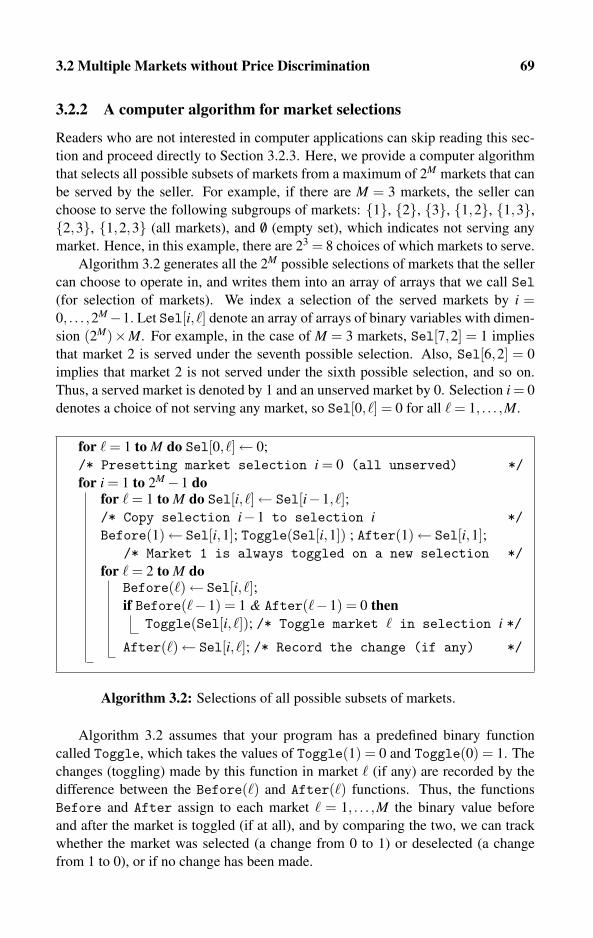
3.2 Multiple Markets without Price Discrimination 69
3.2.2 A computer algorithm for market selections
Readers who are not interested in computer applications can skip reading this sec-
tion and proceed directly to Section 3.2.3. Here, we provide a computer algorithm
that selects all possible subsets of markets from a maximum of 2M markets that can
be served by the seller. For example, if there are M = 3 markets, the seller can
choose to serve the following subgroups of markets: {1}, {2}, {3}, {1,2}, {1,3},{2,3}, {1,2,3} (all markets), and /0 (empty set), which indicates not serving any
market. Hence, in this example, there are 23 = 8 choices of which markets to serve.
Algorithm 3.2 generates all the 2M possible selections of markets that the seller
can choose to operate in, and writes them into an array of arrays that we call Sel(for selection of markets). We index a selection of the served markets by i =0, . . . ,2M−1. Let Sel[i, �] denote an array of arrays of binary variables with dimen-
sion (2M)×M. For example, in the case of M = 3 markets, Sel[7,2] = 1 implies
that market 2 is served under the seventh possible selection. Also, Sel[6,2] = 0
implies that market 2 is not served under the sixth possible selection, and so on.
Thus, a served market is denoted by 1 and an unserved market by 0. Selection i = 0
denotes a choice of not serving any market, so Sel[0, �] = 0 for all � = 1, . . . ,M.
for � = 1 to M do Sel[0, �]← 0;
/* Presetting market selection i = 0 (all unserved) */for i = 1 to 2M−1 do
for � = 1 to M do Sel[i, �]← Sel[i−1, �];/* Copy selection i−1 to selection i */Before(1)← Sel[i,1]; Toggle(Sel[i,1]) ; After(1)← Sel[i,1];
/* Market 1 is always toggled on a new selection */for � = 2 to M do
Before(�)← Sel[i, �];if Before(�−1) = 1 & After(�−1) = 0 then
Toggle(Sel[i, �]); /* Toggle market � in selection i */
After(�)← Sel[i, �]; /* Record the change (if any) */
Algorithm 3.2: Selections of all possible subsets of markets.
Algorithm 3.2 assumes that your program has a predefined binary function
called Toggle, which takes the values of Toggle(1) = 0 and Toggle(0) = 1. The
changes (toggling) made by this function in market � (if any) are recorded by the
difference between the Before(�) and After(�) functions. Thus, the functions
Before and After assign to each market � = 1, . . . ,M the binary value before
and after the market is toggled (if at all), and by comparing the two, we can track
whether the market was selected (a change from 0 to 1) or deselected (a change
from 1 to 0), or if no change has been made.
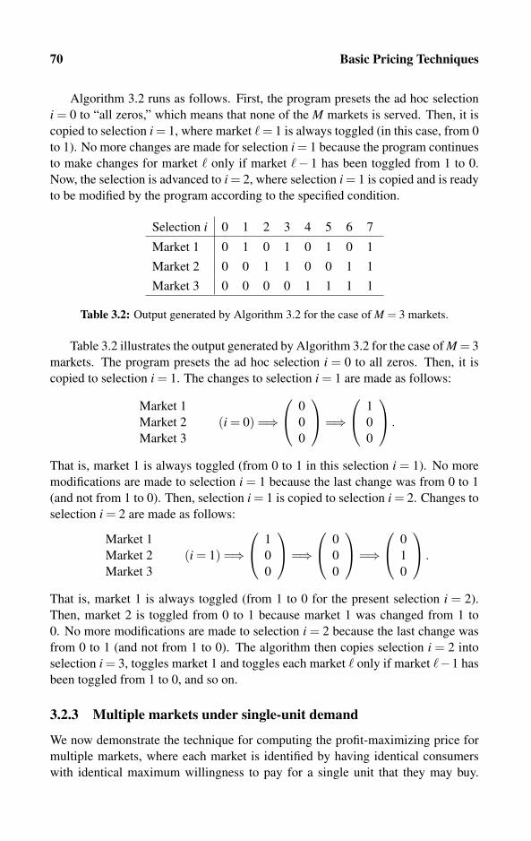
70 Basic Pricing Techniques
Algorithm 3.2 runs as follows. First, the program presets the ad hoc selection
i = 0 to “all zeros,” which means that none of the M markets is served. Then, it is
copied to selection i = 1, where market � = 1 is always toggled (in this case, from 0
to 1). No more changes are made for selection i = 1 because the program continues
to make changes for market � only if market �− 1 has been toggled from 1 to 0.
Now, the selection is advanced to i = 2, where selection i = 1 is copied and is ready
to be modified by the program according to the specified condition.
Selection i 0 1 2 3 4 5 6 7
Market 1 0 1 0 1 0 1 0 1
Market 2 0 0 1 1 0 0 1 1
Market 3 0 0 0 0 1 1 1 1
Table 3.2: Output generated by Algorithm 3.2 for the case of M = 3 markets.
Table 3.2 illustrates the output generated by Algorithm 3.2 for the case of M = 3
markets. The program presets the ad hoc selection i = 0 to all zeros. Then, it is
copied to selection i = 1. The changes to selection i = 1 are made as follows:
Market 1
Market 2
Market 3
(i = 0) =⇒⎛⎝ 0
0
0
⎞⎠=⇒
⎛⎝ 1
0
0
⎞⎠ .
That is, market 1 is always toggled (from 0 to 1 in this selection i = 1). No more
modifications are made to selection i = 1 because the last change was from 0 to 1
(and not from 1 to 0). Then, selection i = 1 is copied to selection i = 2. Changes to
selection i = 2 are made as follows:
Market 1
Market 2
Market 3
(i = 1) =⇒⎛⎝ 1
0
0
⎞⎠=⇒
⎛⎝ 0
0
0
⎞⎠=⇒
⎛⎝ 0
1
0
⎞⎠ .
That is, market 1 is always toggled (from 1 to 0 for the present selection i = 2).
Then, market 2 is toggled from 0 to 1 because market 1 was changed from 1 to
0. No more modifications are made to selection i = 2 because the last change was
from 0 to 1 (and not from 1 to 0). The algorithm then copies selection i = 2 into
selection i = 3, toggles market 1 and toggles each market � only if market �−1 has
been toggled from 1 to 0, and so on.
3.2.3 Multiple markets under single-unit demand
We now demonstrate the technique for computing the profit-maximizing price for
multiple markets, where each market is identified by having identical consumers
with identical maximum willingness to pay for a single unit that they may buy.

3.2 Multiple Markets without Price Discrimination 71
The procedure for aggregating such a demand function has already been studied in
Section 2.5.1.
Three-market example
We start our analysis by working on a three-market example, illustrated by Fig-
ure 3.3. In this example, market 1 has N1 = 200 consumers who will buy the
product/service as long as the price does not exceed $30. Market 2 has N2 = 600
identical consumers who will not pay more than $20, and so on.
�
p
$30
$25
$20
$15
$10
� q1
�
p
$30
$25
$20
$15
$10
� q2
�
p
$30
$25
$20
$15
$10
� q31 1 1
•
•
•
�
p
$30
$25
$20
$15
$10
N1 = 200 N2 = 600 N3 = 200
� q200 400 600 800 1000
•
•
•
Figure 3.3: Single-unit market demand functions with three markets.
The seller has to set a single price p to prevail in all served markets. In this
example, the seller can choose to serve the following subgroups of markets: {1},{2}, {3}, {1,2}, {1,3}, {2,3}, {1,2,3} (all markets), and /0 (empty set), which
indicates not serving any market. In this example, there are 23 = 8 possible selec-
tions of which markets to serve. In the general case of M markets, there are 2M
possibilities to choose from.
Table 3.3 demonstrates how to compute the profit- and revenue-maximizing
prices. In this example, the seller bears a marginal cost of μ = $5; market-specific
fixed costs given by φ1 = $1000, φ2 = $5000, φ3 = 0; and a production fixed
cost of φ = $2000. This example is rather general as it assumes unequal market-
specific fixed costs. For example, the assumption that φ3 = 0 may be a conse-
quence of the firm’s main office being located in the heart of market 3, so no
additional costs of maintaining this market are incurred. Figure 3.3 shows that
if the seller chooses to operate in markets 1 and 3, the price must not exceed
$10 to induce consumers in market 3 to make a purchase. In this case, with
q1,3 = N1 + N3 = 400 customers, the seller’s revenue is x1,3 = $4000. The re-
sulting profit is then y1,3 = (30− 5)400− 1000− 0− 2000 = −$1000. However,
if the seller chooses instead to operate in markets 1 and 2, the price must not ex-
ceed $20 to induce consumers in market 2 to make a purchase. In this case, with

72 Basic Pricing Techniques
Markets 1 2 3 1&2 1&3 2&3 1&2&3
Price $p 30 20 10 20 10 10 10
Quantity q 200 600 200 800 400 800 1000
Revenue $x 6000 12,000 2000 16,000 4000 8000 10,000
(p−μ)q 5000 9000 1000 12,000 2000 4000 5000
Fixed costs 3000 7000 2000 8000 3000 7000 8000
Profit $y 2000 2000 −1000 4000 −1000 −3000 −3000
Table 3.3: Profit-maximizing price when selling to three markets: Single-unit demand
case. Table assumes μ = 5, φ1 = $1000, φ2 = $5000, φ3 = $0, and φ = $2000.
q1,2 = N1 +N2 = 800 customers, the seller’s revenue is x1,2 = $16,000. The result-
ing profit is then y1,2 = (20− 5)800− 1000− 5000− 2000 = $4000, which turns
out to be the maximum profit according to Table 3.3.
A computer algorithm for M markets
We now proceed to describe a computer algorithm for selecting the most profitable
price when there are M markets, and where each market is composed of homo-
geneous consumers with identical maximum willingness to pay, as was already
illustrated in Figure 3.3 for the example of M = 3 markets. The user must run Al-
gorithm 3.2 before running Algorithm 3.3 for the purpose of generating and storing
the 2M possible selections of markets that can be served. Recalling Algorithm 3.2,
the results are stored by the array of arrays of binary variables Sel[i, �] of dimension
2M×M, where i is the index of a specific selection of markets, i = 0,1, . . . ,2M−1,
and � is a specific market. Market � is served under selection i if Sel[i, �] = 1 and
is not served if Sel[i, �] = 0.
The program should read and store the demand structure of each of the M mar-
kets. That is, the program must input (say, using a Read() command) the maximum
willingness to pay V [�] and the number of consumers N[�] (each buying one unit)
for each market � = 1, . . . ,M. V [�] and N[�] are M-dimensional arrays of real and
integer values, respectively. It is recommended to run some trivial loops verifying
nonnegativity. The program must also input the seller’s cost parameters μ (marginal
cost), φ (fixed cost), and the M-dimensional real-valued array of market-specific
fixed costs φ [�] for � = 1, . . . ,M.
The goal of Algorithm 3.3 is to find the profit- and revenue-maximizing selec-
tions of markets out of the 2M possible selections, and the corresponding prices.
These selections are written onto the integer variables maxSy and maxSx, respec-
tively. This algorithm runs a loop over market selections i and computes the profit
and revenue generated by each selection. The profit and revenue are stored on y[i]and x[i]. The price used for these computations is minV [i], which is the lowest max-
imum willingness to pay among all consumers in the selected markets. Note that if

3.2 Multiple Markets without Price Discrimination 73
maxSy← 1; maxSx← 1; /* Initialize: 1st selection */for i = 1 to 2M−1 do minV [i]← 0; y[i]←−φ ; x[i]← 0;
for i = 1 to 2M−1 do/* Main loop over market selections i begins */for � = 1 to M do
/* Maximum chargeable price for market selection i */if minV [i] ·Sel[i, �] > V [�] then minV [i]←V [�];
for � = 1 to M do/* Add profits from all markets under selection i */y[i]← y[i]+{(minV [i]−μ) ·N[�]−φ [�]} ·Sel[i, �];x[i]← x[i]+{minV [i] ·N[�]} ·Sel[i, �]; /* Add revenue */
for i = 1 to 2M−1 doif y[i] > y[maxSy] then maxSy← i; /* i more profitable */if x[i] > x[maxSx] then maxSx← i; /* i higher revenue */
writeln (“The profit-maximizing price is p =”, V [maxSy], “yielding the
profit level y = ”, y[maxSy], “The following markets are served:”);
for � = 1 to M do if Sel[maxSy, �] = 1 then write (“market”, �);
writeln (“The revenue-maximizing price is p =”, V [maxSx], “yielding the
revenue level x = ”, x[maxSx], “The following markets are served:”);
for � = 1 to M do if Sel[maxSy, �] = 1 then write (“market”, �);
Algorithm 3.3: Computing a nondiscriminating monopoly’s profit- and
revenue-maximizing prices under discrete demand with multiple markets.
the firm raises the price above minV [i], the firm will exclude some of the markets,
thereby contradicting the choice of markets made under market selection i.The remainder of Algorithm 3.3 consists of a loop for determining the profit-
and revenue-maximizing selections of markets. These selections are written onto
the integer variables maxSy and maxSx, respectively. For these selections of mar-
kets, the algorithm then writes the corresponding prices, and the list of served mar-
kets under these prices.
3.2.4 Linear demand: Example for two markets
We now leave the discrete demand case and proceed to analyze continuous demand
functions. First, consider two markets described by the inverse demand functions
p1 = 100−0.5q1 and p2 = 50−0.1q2. (3.15)
The market-specific fixed cost associated with operating in markets 1 and 2 are
φ1 = φ2 = $500. In addition, the fixed cost associated with the operation of the
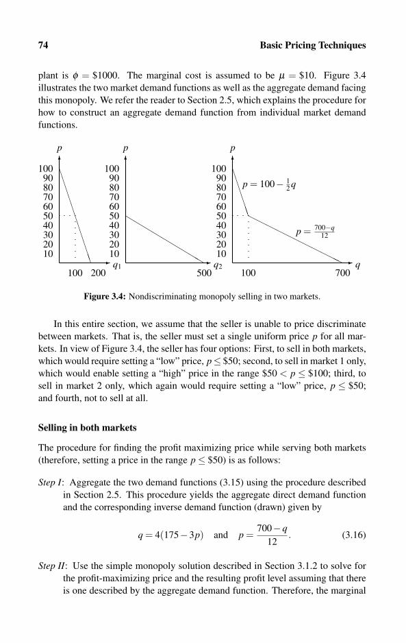
74 Basic Pricing Techniques
plant is φ = $1000. The marginal cost is assumed to be μ = $10. Figure 3.4
illustrates the two market demand functions as well as the aggregate demand facing
this monopoly. We refer the reader to Section 2.5, which explains the procedure for
how to construct an aggregate demand function from individual market demand
functions.
� q1200
102030405060708090
100� �
p p
�����������
102030405060708090
100
q2�
�
p
102030405060708090
100
100 100
������
700
�
���������
500
p = 100− 12q
p = 700−q12
q
Figure 3.4: Nondiscriminating monopoly selling in two markets.
In this entire section, we assume that the seller is unable to price discriminate
between markets. That is, the seller must set a single uniform price p for all mar-
kets. In view of Figure 3.4, the seller has four options: First, to sell in both markets,
which would require setting a “low” price, p≤ $50; second, to sell in market 1 only,
which would enable setting a “high” price in the range $50 < p ≤ $100; third, to
sell in market 2 only, which again would require setting a “low” price, p ≤ $50;
and fourth, not to sell at all.
Selling in both markets
The procedure for finding the profit maximizing price while serving both markets
(therefore, setting a price in the range p≤ $50) is as follows:
Step I: Aggregate the two demand functions (3.15) using the procedure described
in Section 2.5. This procedure yields the aggregate direct demand function
and the corresponding inverse demand function (drawn) given by
q = 4(175−3p) and p =700−q
12. (3.16)
Step II: Use the simple monopoly solution described in Section 3.1.2 to solve for
the profit-maximizing price and the resulting profit level assuming that there
is one described by the aggregate demand function. Therefore, the marginal
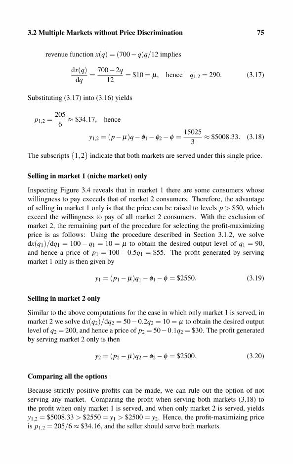
3.2 Multiple Markets without Price Discrimination 75
revenue function x(q) = (700−q)q/12 implies
dx(q)dq
=700−2q
12= $10 = μ , hence q1,2 = 290. (3.17)
Substituting (3.17) into (3.16) yields
p1,2 =205
6≈ $34.17, hence
y1,2 = (p−μ)q−φ1−φ2−φ =15025
3≈ $5008.33. (3.18)
The subscripts {1,2} indicate that both markets are served under this single price.
Selling in market 1 (niche market) only
Inspecting Figure 3.4 reveals that in market 1 there are some consumers whose
willingness to pay exceeds that of market 2 consumers. Therefore, the advantage
of selling in market 1 only is that the price can be raised to levels p > $50, which
exceed the willingness to pay of all market 2 consumers. With the exclusion of
market 2, the remaining part of the procedure for selecting the profit-maximizing
price is as follows: Using the procedure described in Section 3.1.2, we solve
dx(q1)/dq1 = 100− q1 = 10 = μ to obtain the desired output level of q1 = 90,
and hence a price of p1 = 100− 0.5q1 = $55. The profit generated by serving
market 1 only is then given by
y1 = (p1−μ)q1−φ1−φ = $2550. (3.19)
Selling in market 2 only
Similar to the above computations for the case in which only market 1 is served, in
market 2 we solve dx(q2)/dq2 = 50−0.2q2 = 10 = μ to obtain the desired output
level of q2 = 200, and hence a price of p2 = 50−0.1q2 = $30. The profit generated
by serving market 2 only is then
y2 = (p2−μ)q2−φ2−φ = $2500. (3.20)
Comparing all the options
Because strictly positive profits can be made, we can rule out the option of not
serving any market. Comparing the profit when serving both markets (3.18) to
the profit when only market 1 is served, and when only market 2 is served, yields
y1,2 = $5008.33 > $2550 = y1 > $2500 = y2. Hence, the profit-maximizing price
is p1,2 = 205/6≈ $34.16, and the seller should serve both markets.

76 Basic Pricing Techniques
3.2.5 Linear demand: General formulation for two markets
We now provide the general formulation of the two-market example for general
linear demand functions. Let the demand functions for markets 1 and 2 be given by
p1 = α1−β1q1 and p2 = α2−β2q2, where α1 > μ ≥ 0 and α2 > μ . We now follow
exactly the same steps as in Section 3.2.4 to find the seller’s profit-maximizing
price.
Using the procedure described in Section 2.5, the aggregate direct demand
function and the corresponding inverse demand function are given by
q =α1β2 +α2β1− (β1 +β2)p
β1β2and p =
α1β2 +α2β1−β1β2qβ1 +β2
. (3.21)
Using the procedure described in Section 3.1.2, we solve
dx(q)dq
=α1β2 +α2β1−2β1β2q
β1 +β2= μ , yielding
q1,2 =α1β2 +α2β1− (β1 +β2)μ
2β1β2. (3.22)
Substituting (3.22) into (3.21) yields
p1,2 =α1β2 +α2β1 +(β1 +β2)μ
2(β1 +β2)hence y1,2 = (p1,2−μ)q1,2−φ1−φ2−φ
=[α1β2 +α2β1−μ(β1 +β2)]
2
4β1β2(β1 +β2)−φ1−φ2−φ . (3.23)
We now solve for the profit-maximizing price assuming that only market 1 is
served. Thus, solving dx(q1)/dq1 = α1− 2β1q1 = μ yields a desired output level
of q1 = (α1− μ)/(2β1) and a price of p1 = (α1 + μ)/2. The profit generated by
serving market 1 only is then
y1 = (p1−μ)q1−φ1−φ =(α1−μ)2
4β1−φ1−φ . (3.24)
Similarly, when only market 2 is served, solving dx(q2)/dq2 = α2−β2q2 = μyields a desired output level of q2 = (α2− μ)/(2β2), therefore a price of p2 =(α2 + μ)/2. The profit generated by serving market 2 only is then
y2 = (p2−μ)q2−φ2−φ =(α2−μ)2
4β2−φ2−φ . (3.25)
Finally, to be able to select which markets are served, we must compare the
profit when serving both markets (3.23) to the profit when only market 1 is served
(3.24), and when only market 2 is served (3.24), and then set the price-maximizing
price accordingly.

3.2 Multiple Markets without Price Discrimination 77
3.2.6 Linear demand: A computer algorithm for multiple markets
Our next generalization extends the previous analysis to any number of markets,
each represented by a linear demand function. Our analysis assumes M markets,
indexed by � = 1,2, . . .M. Each market is characterized by a downward-sloping
inverse linear demand function p� = α�−β� q�, where α�,β� > 0 are to be estimated
from actual market-specific data, using the procedure studied in Section 2.3.2.
The general principle for selecting the profit-maximizing price is to go over all
the i = 0,1, . . . ,2M−1 selections of subsets of markets (including the option of not
selling in any market) and then to compare the resulting profit levels. There can
be two types of computer algorithms for solving the nondiscriminating monopoly
problem selling in multiple markets. One algorithm, which resembles symbolic
algebra software, follows exactly the steps described in the previous paragraph.
Such an algorithm must read the demand parameters α� and β� for all markets
� = 1, . . . ,M, and combine these parameters to construct the aggregate demand
function corresponding to the exact choice of markets to be served. The advantage
of this type of algorithm is that it computes the exact profit-maximizing price with-
out resorting to an approximation that is sensitive to the precision or grid that must
be specified for the loops over price changes. In this section, we take a slightly
different approach. For each selection of markets, the proposed algorithm starts
from a high price and then gradually decreases the price and computes the profit
generated from serving the selected markets. The price reductions depend on the
grid, which the user must input into the parameter G. This precision parameter
(again, set by the user) determines the degree of accuracy of this computation.
Algorithm 3.4 requires first running Algorithm 3.2, which lists and writes all the
2M possible selections of subsets of M markets onto the array of arrays of binary
variables Sel[i, �], where i is the index number of a specific selection of markets
and � is a specific market. As before, Sel[i, �] = 1 indicates that market � is se-
lected under selection i, whereas Sel[i, �] = 0 indicates that market � is excluded.
Then, similar to Algorithm 3.3, Algorithm 3.4 computes the profit for each selec-
tion of markets by comparing the maximum profit from each selection of markets
i. However, because the demand is downward sloping, Algorithm 3.4 must run
an additional loop over price p (see the “While” loop) by varying the price (with
increments determined by the inputted grid parameter G) and then computing the
profit for each price p.
The program should read and store the demand structure of each of M markets.
That is, the program must input (say, using a Read() command) the inverse demand
intercept α[�] and the slope β [�] parameters for each market � = 1, . . . ,M. It is
recommended to run some trivial loops verifying nonnegativity and that α[�] > μ(thereby verifying that the willingness to pay for some consumers in each mar-
ket exceeds marginal cost), as otherwise market � can be immediately excluded.
The program must also input the seller’s cost parameters μ (marginal cost), φ
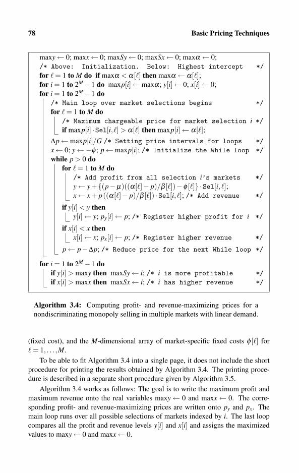
78 Basic Pricing Techniques
maxy← 0; maxx← 0; maxSy← 0; maxSx← 0; maxα ← 0;
/* Above: Initialization. Below: Highest intercept */for � = 1 to M do if maxα < α[�] then maxα ← α[�];for i = 1 to 2M−1 do maxp[i]←maxα; y[i]← 0; x[i]← 0;
for i = 1 to 2M−1 do/* Main loop over market selections begins */for � = 1 to M do
/* Maximum chargeable price for market selection i */if maxp[i] ·Sel[i, �] > α[�] then maxp[i]← α[�];
Δp←maxp[i]/G /* Setting price intervals for loops */x← 0; y←−φ ; p←maxp[i]; /* Initialize the While loop */while p > 0 do
for � = 1 to M do/* Add profit from all selection i’s markets */y← y+{(p−μ)((α[�]− p)/β [�])−φ [�]} ·Sel[i, �];x← x+ p((α[�]− p)/β [�]) ·Sel[i, �]; /* Add revenue */
if y[i] < y theny[i]← y; py[i]← p; /* Register higher profit for i */
if x[i] < x thenx[i]← x; px[i]← p; /* Register higher revenue */
p← p−Δp; /* Reduce price for the next While loop */
for i = 1 to 2M−1 doif y[i] > maxy then maxSy← i; /* i is more profitable */if x[i] > maxx then maxSx← i; /* i has higher revenue */
Algorithm 3.4: Computing profit- and revenue-maximizing prices for a
nondiscriminating monopoly selling in multiple markets with linear demand.
(fixed cost), and the M-dimensional array of market-specific fixed costs φ [�] for
� = 1, . . . ,M.
To be able to fit Algorithm 3.4 into a single page, it does not include the short
procedure for printing the results obtained by Algorithm 3.4. The printing proce-
dure is described in a separate short procedure given by Algorithm 3.5.
Algorithm 3.4 works as follows: The goal is to write the maximum profit and
maximum revenue onto the real variables maxy← 0 and maxx← 0. The corre-
sponding profit- and revenue-maximizing prices are written onto py and px. The
main loop runs over all possible selections of markets indexed by i. The last loop
compares all the profit and revenue levels y[i] and x[i] and assigns the maximized
values to maxy← 0 and maxx← 0.

3.3 Multiple Markets with Price Discrimination 79
writeln (“The profit-maximizing price is p =”, py, “yielding the profit level
y = ”, y[maxSy], “The following markets are served:”);
for � = 1 to M do if Sel[maxSy, �] = 1 then write (“market”, �);
writeln (“The revenue-maximizing price is p =”, px, “yielding the revenue
level x = ”, x[maxSx], “The following markets are served:”);
for � = 1 to M do if Sel[maxSx, �] = 1 then write (“market”, �);
Algorithm 3.5: Printing the output of Algorithm 3.4.
The main inner “While” loop runs over all possible prices (given the specified
precision) for each selection of markets i. The price starts at the highest demand
intercept maxp[i] (which is the highest demand intercept for this specific selection
of markets). For each price, the corresponding profit and revenue levels are written
onto the real temporary variables y and x. If the price generates higher levels for
these, variables are then assigned to the maximum profit and revenue for selection i,y[i] and x[i]. The “While” loop ends where the price is reduced by Δp, and the loop
continues as long as the price is strictly positive.
3.3 Multiple Markets with Price Discrimination
The ability to price discriminate means that the seller can set different prices in
different markets. Setting different prices is possible only if the markets are seg-
mented in the sense that arbitrage (buying at the low-priced market for the purpose
of reselling at the high-priced market) is not feasible. The reader is referred to Sec-
tion 1.2 for extensive discussions of market segmentation and price discrimination.
We therefore proceed directly to analyzing pricing techniques. We divide our anal-
ysis into situations in which the seller has sufficient capacity to satisfy the demand
in all markets, and situations in which capacity is limited.
3.3.1 Unlimited capacity: Linear demand
Two-market example
We start with the two-market example that we analyzed earlier in Section 3.2.4 for
the case in which the seller is unable to price discriminate. Recalling the demand
functions (3.15),
p1 = 100−0.5q1 and p2 = 50−0.1q2. (3.26)
Figure 3.5 draws the demand functions (3.26) and the corresponding marginal rev-
enue functions for each market. Section 2.3.3 has already demonstrated how to
derive the marginal revenue functions associated with linear demand functions.
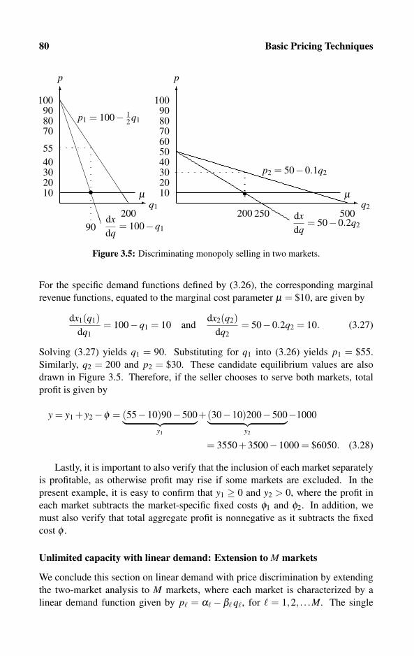
80 Basic Pricing Techniques
10203040
708090
100�
p�
p
102030405060708090
100
�
200q1
������������
��������������
500250
� q2
dxdq
= 50−0.2q2dxdq
= 100−q1
μμ
200
90
••
55
p1 = 100− 12q1
p2 = 50−0.1q2
Figure 3.5: Discriminating monopoly selling in two markets.
For the specific demand functions defined by (3.26), the corresponding marginal
revenue functions, equated to the marginal cost parameter μ = $10, are given by
dx1(q1)dq1
= 100−q1 = 10 anddx2(q2)
dq2= 50−0.2q2 = 10. (3.27)
Solving (3.27) yields q1 = 90. Substituting for q1 into (3.26) yields p1 = $55.
Similarly, q2 = 200 and p2 = $30. These candidate equilibrium values are also
drawn in Figure 3.5. Therefore, if the seller chooses to serve both markets, total
profit is given by
y = y1 + y2−φ = (55−10)90−500︸ ︷︷ ︸y1
+(30−10)200−500︸ ︷︷ ︸y2
−1000
= 3550+3500−1000 = $6050. (3.28)
Lastly, it is important to also verify that the inclusion of each market separately
is profitable, as otherwise profit may rise if some markets are excluded. In the
present example, it is easy to confirm that y1 ≥ 0 and y2 > 0, where the profit in
each market subtracts the market-specific fixed costs φ1 and φ2. In addition, we
must also verify that total aggregate profit is nonnegative as it subtracts the fixed
cost φ .
Unlimited capacity with linear demand: Extension to M markets
We conclude this section on linear demand with price discrimination by extending
the two-market analysis to M markets, where each market is characterized by a
linear demand function given by p� = α�− β� q�, for � = 1,2, . . .M. The single

3.3 Multiple Markets with Price Discrimination 81
seller bears a constant marginal cost of μ , market-specific fixed cost of φ� for � =1,2, . . .M, and production fixed cost of φ . The seller must decide in which markets
to operate and the price for each market. To solve this problem, the seller should
use the following two-step procedure:
Step I: For each market �, solve
dx(q�)dq�
= α�−2β� q� = μ , yielding q� =α�−μ
2β�and p� =
α� + μ2
.
The price p� for market � was obtained by substituting q� into the demand
function in market �.
Step II: Compute the profit generated from each market � to obtain
y� = (p�−μ)q�−φ� =(α�−μ)2
4β�−φ�,
and choose to serve only the markets for which y� ≥ 0. Lastly, add all profits
generated from all served markets and subtract the production fixed cost φ to
obtain total profit.
Unlimited capacity with linear demand: Computer algorithm
We now provide a simple computer algorithm for selecting the profit-maximizing
price for each market, and for selecting the markets to be served. Algorithm 3.6
assumes that the program already stores the linear demand parameters for each of
the M markets. Thus, the program must input the demand intercept α[�] and the
slope parameter β [�] for each inverse demand function indexed by � = 1, . . . ,M. It
is recommended to run some trivial loops verifying that α� > 0 and that −β� < 0.
The program must also input the seller’s cost parameters μ (marginal cost), the
market-specific fixed costs φ [�], and the fixed production cost φ .
Algorithm 3.6 is rather straightforward. It runs a loop on all markets � =1,2, · · · ,M, and computes the profit level. If the profit from market � (after sub-
tracting the market specific fixed cost φ [�]) is nonnegative, it selects market � by
assigning 1 to Sel[�], which is an array of binary variables of dimension M. Total
output and total profit are added to the aggregate levels represented by the real vari-
ables y and q. Finally, note that Algorithm 3.6 also computes the aggregate output
level q. This quantity will become very important when we analyze capacity con-
straints in Section 3.3.3, as this level will have to be compared with the available
capacity to check whether the capacity is binding.
3.3.2 Unlimited capacity: Constant-elasticity demand
The procedure for selecting the profit-maximizing price when the seller faces a
constant elasticity demand function has already been analyzed in Section 3.1.4 for
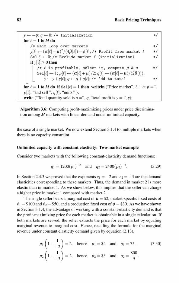
82 Basic Pricing Techniques
y←−φ ; q← 0; /* Initialization */for � = 1 to M do
/* Main loop over markets */y[�]← (α[�]−μ)2/(4β [�])−φ [�]; /* Profit from market � */Sel[�]← 0; /* Exclude market � (initialization) */if y[�]≥ 0 then
/* � is profitable, select it, compute p & q */Sel[�]← 1; p[�]← (α[�]+ μ)/2; q[�]← (α[�]−μ)/(2β [�]);
y← y+ y[�]; q← q+q[�]; /* Add to total */
for � = 1 to M do if Sel[�] = 1 then writeln (“Price market”, �, “ at p =”,
p[�], “and sell ”, q[�], “units.” );
write (“Total quantity sold is q =”, q, “total profit is y = ”, y);
Algorithm 3.6: Computing profit-maximizing prices under price discrimina-
tion among M markets with linear demand under unlimited capacity.
the case of a single market. We now extend Section 3.1.4 to multiple markets when
there is no capacity constraint.
Unlimited capacity with constant elasticity: Two-market example
Consider two markets with the following constant-elasticity demand functions:
q1 = 1200(p1)−2 and q2 = 2400(p2)−3. (3.29)
In Section 2.4.3 we proved that the exponents e1 =−2 and e2 =−3 are the demand
elasticities corresponding to these markets. Thus, the demand in market 2 is more
elastic than in market 1. As we show below, this implies that the seller can charge
a higher price in market 1 compared with market 2.
The single seller bears a marginal cost of μ = $2, market-specific fixed costs of
φ1 = $100 and φ2 = $50, and a production fixed cost of φ = $30. As we have shown
in Section 3.1.4, the advantage of working with a constant-elasticity demand is that
the profit-maximizing price for each market is obtainable in a single calculation. If
both markets are served, the seller extracts the price for each market by equating
marginal revenue to marginal cost. Hence, recalling the formula for the marginal
revenue under constant elasticity demand given by equation (2.13),
p1
(1+
1
−2
)= 2, hence p1 = $4 and q1 = 75, (3.30)
p2
(1+
1
−3
)= 2, hence p2 = $3 and q2 =
800
9.

3.3 Multiple Markets with Price Discrimination 83
Therefore, if the seller chooses to serve both markets, total profit is given by
y = y1 + y2−φ = (4−2)75−100︸ ︷︷ ︸y1
+(3−2)800
9−50︸ ︷︷ ︸
y2
−30
= 50+350
9−30 =
530
9≈ $58.88. (3.31)
Lastly, it is important to verify that the inclusion of each market separately is prof-
itable, as otherwise it may be profitable to exclude some markets. In the present
example, we indeed verify that y1 ≥ 0 and y2 > 0, where these market-specific
profits already subtract the market-specific fixed costs φ1 and φ2. In addition, we
must verify that total profit is nonnegative once the fixed cost φ is also taken into
account.
The two first-order conditions for profit maximization (3.30) demonstrate why
constant-elasticity demand functions are so easy to use for the purpose of selecting
the profit-maximizing prices in different markets. In fact, we can show from these
conditions that it is sufficient to know only the value of the demand elasticities in
each market to be able to tell the profit-maximizing price ratio between any two
served markets. Thus, very little information is required to be able to compute the
profit-maximizing price ratios. To see this, suppose that you obtain the information
that the demand price elasticity in market 1 is a constant given by e1. Similarly,
for market 2, the price elasticity is e2. Note that we must assume elastic demand,
e1 <−1 and e2 <−1, as we have already proved that a monopoly will never charge
a price at a point at which the demand is inelastic. Using this information only (yes,
even without knowing the value of the marginal cost μ), we can compute that
p1
(1+
1
e1
)= μ = p2
(1+
1
e2
), hence
p1
p2=
e1(e2 +1)e2(e1 +1)
. (3.32)
For example, if e1 =−2 and e2 =−3, the profit-maximizing price ratio is p1/p2 =4/3, which also reconfirms our earlier computation given in (3.30). Similarly, if
e1 = −2 and e2 = −4, the profit-maximizing price ratio is p1/p2 = 3/2. For this
last example, this ratio implies that the seller should set prices so that the price in
market 1 is 50% higher than the price in market 2.
Unlimited capacity with constant elasticity: Extension to M markets
We conclude this section on constant-elasticity demand with price discrimination
under unlimited capacity by extending the two-market analysis to M markets, where
each market � = 1,2, . . .M is characterized by a constant-elasticity demand func-
tion given by q� = α� p−β� . The single seller bears a constant marginal cost of μ ,
a market-specific fixed cost of φ� for � = 1,2, . . .M, and a production fixed cost of
φ . The seller must decide in which market to operate and the price for each served

84 Basic Pricing Techniques
market. To solve this problem, the seller should follow the following two-step pro-
cedure:
Step I: For each market �, solve
dx(q�)dq�
= p�
(1+
1
β�
)= μ yielding
p� =β� μ
β�−1and q� = α�
(β� μ
β�−1
)−β�
.
The output level q� was obtained by substituting p� into the direct demand
function in market �.
Step II: Compute the profit from each market � to obtain
y� = (p�−μ)q�−φ� = α�
(β� μ
β�−1
)1−β�
−φ�,
and choose to serve only the markets for which y� ≥ 0. Lastly, add all profits
from all served markets and subtract the production fixed cost φ to obtain
total profit.
3.3.3 Price discrimination under capacity constraint
Our analysis so far in this chapter has implicitly assumed that the seller/producer
possesses the capacity of satisfying the entire demand when prices are set at the
profit-maximizing level. Clearly, this is not always the case. For example, airlines
have a limited seating capacity during high travel seasons. Hotels often face similar
limitations on the number of rooms they can rent out. Therefore, in this section we
assume that the seller faces a capacity constraint K in the sense that it cannot serve
more than K customers (or sell more than K units). Notice that we denote capacity
with a capital letter K to indicate that the capacity level is treated as an exogenously
given parameter, corresponding to the list of parameters given in Table 1.4. In
general, there are two ways of interpreting the capacity level K:
(a) Capacity has not been paid for: In this case, the seller must bear a marginal
cost, denoted by μk for each additional unit of capacity, bringing the total ca-
pacity to μkK.
(b) The seller has already paid for it: Cost of capacity should be regarded as sunk.
Our analysis below captures both situations. If capacity has already been paid for,
then the entire cost should be incorporated in the fixed cost parameter φ . Otherwise,
if capacity has to be purchased for generating higher output levels, capacity cost
should be incorporated in the marginal cost parameter μk. Generally, managers are
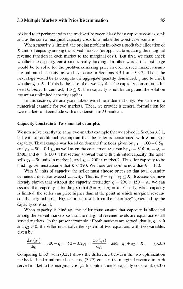
3.3 Multiple Markets with Price Discrimination 85
advised to experiment with the trade-off between classifying capacity cost as sunk
and as the sum of marginal capacity costs to simulate the worst-case scenario.
When capacity is limited, the pricing problem involves a profitable allocation of
K units of capacity among the served markets (as opposed to equating the marginal
revenue function in each market to the marginal cost). But first, we must check
whether the capacity constraint is really binding. In other words, the first stage
would be to solve for the profit-maximizing price in each served market assum-
ing unlimited capacity, as we have done in Sections 3.3.1 and 3.3.2. Then, the
next stage would be to compute the aggregate quantity demanded, q and to check
whether q > K. If this is the case, then we say that the capacity constraint is in-
deed binding. In contrast, if q ≤ K, then capacity is not binding, and the solution
assuming unlimited capacity applies.
In this section, we analyze markets with linear demand only. We start with a
numerical example for two markets. Then, we provide a general formulation for
two markets and conclude with an extension to M markets.
Capacity constraint: Two-market examples
We now solve exactly the same two-market example that we solved in Section 3.3.1,
but with an additional assumption that the seller is constrained with K units of
capacity. That example was based on demand functions given by p1 = 100−0.5q1
and p2 = 50−0.1q2, as well as on the cost structure given by μ = $10, φ1 = φ2 =$500, and φ = $1000. That section showed that with unlimited capacity, the seller
sells q1 = 90 units in market 1, and q2 = 200 in market 2. Thus, for capacity to be
binding, we must assume that K < 290. We therefore assume now that K = 150.
With K units of capacity, the seller must choose prices so that total quantity
demanded does not exceed capacity. That is, q = q1 + q2 ≤ K. Because we have
already shown that without the capacity restriction q = 290 > 150 = K, we can
assume that capacity is binding so that q = q1 + q2 = K. Clearly, when capacity
is limited, the seller can price higher than at the point at which marginal revenue
equals marginal cost. Higher prices result from the “shortage” generated by the
capacity constraint.
When capacity is binding, the seller must ensure that capacity is allocated
among the served markets so that the marginal revenue levels are equal across all
served markets. In the present example, if both markets are served, that is, q1 > 0
and q2 > 0, the seller must solve the system of two equations with two variables
given by
dx1(q1)dq1
= 100−q1 = 50−0.2q2 =dx2(q2)
dq2and q1 +q2 = K. (3.33)
Comparing (3.33) with (3.27) shows the difference between the two optimization
methods. Under unlimited capacity, (3.27) equates the marginal revenue in each
served market to the marginal cost μ . In contrast, under capacity constraint, (3.33)

86 Basic Pricing Techniques
reveals that the marginal cost μ does not explicitly enter into the optimization’s
marginal condition as this condition requires that only marginal costs in all served
markets will be equalized to a level that may exceed the marginal cost μ , and that
in addition total output should be set to equal the given capacity level K.
Solving (3.33) for q1 and q2 yields
q1 =200
3and q2 =
250
3, hence p1 =
200
3and p2 =
125
3. (3.34)
The prices p1 and p2 were obtained by substituting the profit-maximizing output
levels q1 and q2 into the corresponding market inverse demand functions. Clearly,
by construction, total output equals capacity so that q1 +q2 = 150 = K. The result-
ing total profit is then given by
y1 =(
200
3−10
)200
3−500 =
29500
9≈ $3277 > 0, (3.35)
y2 =(
250
3−10
)250
3−500 =
19250
9≈ $2138 > 0.
Hence, total profit is given by y = y1 + y2−1000 = 13,250/3≈ $4416 > 0. Alto-
gether, because both markets are profitable, and because total profit is also nonneg-
ative, the prices given in (3.34) are indeed the profit-maximizing prices.
The above analysis turned out to be very simple because the capacity constraint
was sufficiently large to make it profitable to operate in both markets. However,
as we now demonstrate, for a sufficiently low capacity level, the introduction of a
capacity constraint may induce the seller to exclude some markets. To demonstrate
this possibility, let us “reduce” the amount of available capacity to K = 40 (down
from K = 150). If we attempt to naively solve the two equations (3.33) we obtain
q1 = 145/3 and q2 = −25/3 < 0. This means that market 2 should not be served.
Indeed, inspecting Figure 3.5 reveals that with only K = 40 units of capacity, by
selling in market 1 only the seller can charge a much higher price than the price
that can be charged if selling also in market 2.
To complete this example with K = 40 units of capacity, selling in market 1
only implies that q1 = K = 40, hence, p1 = 100− 0.5 · 40 = $80. Therefore, y =y1−φ = (80−10)40−500−1000 = $1300.
Capacity constraint with two markets: General formulation
We now reformulate the above two-market example to generalize it to any linear
demand function given by p1 = α1−β1q1 and p2 = α2−β2q2, where the param-
eters α1, α2, β1, and β2 are nonnegative, to be estimated by the econometrician
as demonstrated in Section 2.3.2. To find the profit-maximizing prices and which
markets should be served, the manager should follow the following steps:
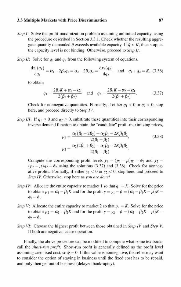
3.3 Multiple Markets with Price Discrimination 87
Step I: Solve the profit-maximization problem assuming unlimited capacity, using
the procedure described in Section 3.3.1. Check whether the resulting aggre-
gate quantity demanded q exceeds available capacity. If q < K, then stop, as
the capacity level is not binding. Otherwise, proceed to Step II.
Step II: Solve for q1 and q2 from the following system of equations,
dx1(q1)dq1
= α1−2β1q1 = α2−2β2q2 =dx2(q2)
dq2and q1 +q2 = K, (3.36)
to obtain
q1 =2β2K +α1−α2
2(β1 +β2)and q2 =
2β1K +α2−α1
2(β1 +β2). (3.37)
Check for nonnegative quantities. Formally, if either q1 < 0 or q2 < 0, stop
here, and proceed directly to Step IV.
Step III: If q1 ≥ 0 and q2 ≥ 0, substitute these quantities into their corresponding
inverse demand function to obtain the “candidate” profit-maximizing prices,
p1 =α1(β1 +2β2)+α2β1−2Kβ1β2
2(β1 +β2), (3.38)
p2 =α2(2β1 +β2)+α1β2−2Kβ1β2
2(β1 +β2).
Compute the corresponding profit levels y1 = (p1 − μ)q1 − φ1 and y2 =(p2− μ)q2− φ2 using the solutions (3.37) and (3.38). Check for nonneg-
ative profits. Formally, if either y1 < 0 or y2 < 0, stop here, and proceed to
Step IV. Otherwise, stop here as you are done!
Step IV: Allocate the entire capacity to market 1 so that q1 = K. Solve for the price
to obtain p1 = α1−β1K and for the profit y = y1−φ = (α1−β1K−μ)K−φ1−φ .
Step V: Allocate the entire capacity to market 2 so that q2 = K. Solve for the price
to obtain p2 = α2−β2K and for the profit y = y2−φ = (α2−β2K−μ)K−φ2−φ .
Step VI: Choose the highest profit between those obtained in Step IV and Step V.
If both are negative, cease operation.
Finally, the above procedure can be modified to compute what some textbooks
call the short-run profit. Short-run profit is generally defined as the profit level
assuming zero fixed cost, so φ = 0. If this value is nonnegative, the seller may want
to consider the option of staying in business until the fixed cost has to be repaid,
and only then get out of business (delayed bankruptcy).
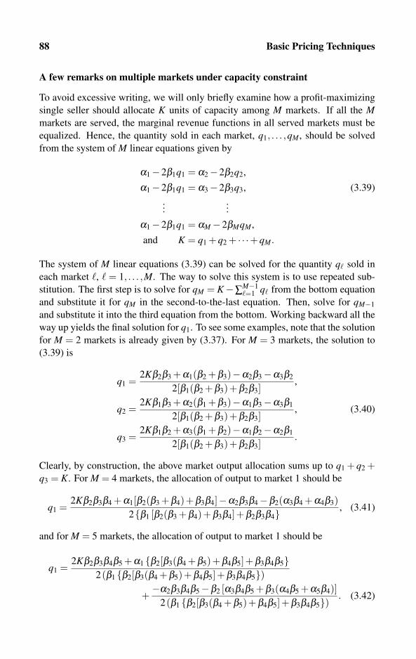
88 Basic Pricing Techniques
A few remarks on multiple markets under capacity constraint
To avoid excessive writing, we will only briefly examine how a profit-maximizing
single seller should allocate K units of capacity among M markets. If all the Mmarkets are served, the marginal revenue functions in all served markets must be
equalized. Hence, the quantity sold in each market, q1, . . . ,qM, should be solved
from the system of M linear equations given by
α1−2β1q1 = α2−2β2q2,
α1−2β1q1 = α3−2β3q3, (3.39)
......
α1−2β1q1 = αM−2βMqM,
and K = q1 +q2 + · · ·+qM.
The system of M linear equations (3.39) can be solved for the quantity q� sold in
each market �, � = 1, . . . ,M. The way to solve this system is to use repeated sub-
stitution. The first step is to solve for qM = K−∑M−1�=1 q� from the bottom equation
and substitute it for qM in the second-to-the-last equation. Then, solve for qM−1
and substitute it into the third equation from the bottom. Working backward all the
way up yields the final solution for q1. To see some examples, note that the solution
for M = 2 markets is already given by (3.37). For M = 3 markets, the solution to
(3.39) is
q1 =2Kβ2β3 +α1(β2 +β3)−α2β3−α3β2
2[β1(β2 +β3)+β2β3],
q2 =2Kβ1β3 +α2(β1 +β3)−α1β3−α3β1
2[β1(β2 +β3)+β2β3], (3.40)
q3 =2Kβ1β2 +α3(β1 +β2)−α1β2−α2β1
2[β1(β2 +β3)+β2β3].
Clearly, by construction, the above market output allocation sums up to q1 + q2 +q3 = K. For M = 4 markets, the allocation of output to market 1 should be
q1 =2Kβ2β3β4 +α1[β2(β3 +β4)+β3β4]−α2β3β4−β2(α3β4 +α4β3)
2{β1 [β2(β3 +β4)+β3β4]+β2β3β4} , (3.41)
and for M = 5 markets, the allocation of output to market 1 should be
q1 =2Kβ2β3β4β5 +α1 {β2[β3(β4 +β5)+β4β5]+β3β4β5}
2(β1 {β2[β3(β4 +β5)+β4β5]+β3β4β5})+−α2β3β4β5−β2 [α3β4β5 +β3(α4β5 +α5β4)]
2(β1 {β2[β3(β4 +β5)+β4β5]+β3β4β5}) . (3.42)

3.4 Pricing under Competition 89
Recall however that the solutions given by (3.37), (3.40), (3.41), and (3.42) may
yield negative values for output levels. That is, the repeated substitution method
for solving the system of equations (3.39) may yield negative values. In such cases,
the markets with “negative output levels” should be excluded one by one, and the
resulting reduced systems should be recomputed for the smaller number of markets.
In general, the method of allocating K units of capacity to M markets should adhere
to the following steps:
Step I: Solve the profit-maximization problem assuming unlimited capacity, using
the procedure described in Section 3.3.1. Check whether the resulting aggre-
gate quantity demanded q exceeds available capacity. If q < K, then stop, as
the capacity level is not binding. Otherwise, proceed to Step II.
Step II: Run Algorithm 3.2, which lists all the i = 1, . . . ,2M possible selections of
subsets of markets.
Step III: Similar to the system of equations (3.39), solve the system of equations
corresponding to each selection i of subsets of markets. Check whether the
solution yields nonnegative output levels in some of the markets � = 1, . . . ,M.
If negative output is found in some of the markets in selection i, selection ishould be ruled out.
Step IV: Compare total profit from each selection of markets i to determine which
markets should be served. Substitute the corresponding output levels into the
demand function of each selected market to determine the profit-maximizing
price to be charged in each selected market.
3.4 Pricing under Competition
In this section we briefly address the issue of competition. Firms’ strategic behavior
under competition constitutes the core study of industrial organization, which is a
field of study in modern economics. For this reason, a comprehensive study of
firms’ behavior under competition is beyond the scope of this book. Readers who
are interested in learning theories of market structures should consult a wide variety
of industrial organization textbooks. By market structure economists refer to the
precise “rules of the game” (yes, just like the game of chess) which describe what
actions (such as prices and quantity produced) firms are “allowed” to take when
competing with other firms.
There are two alternative approaches that must be considered when setting a
price in a market where several competing firms operate.
Myopic rival firms: This approach assumes that rival firms will not respond to price
changes made by other firms. Thus, the firm in question views the prices set
by its rivals as constants, at least in the short run.

90 Basic Pricing Techniques
Strategic rival firms: Firms respond to any price changes made by their rivals. Un-
der this approach, economists define various types of equilibria (or market
structures). The most commonly used equilibrium concept is the Nash-
Bertrand equilibrium, which consists of a vector of prices (one for each firm)
under which no firm finds it profitable to deviate from these prices as long as
other firms do not deviate.
As mentioned above, strategic behavior of firms has been the main focus of study
by economists in the past 30 years and therefore will be given little attention in
this book. Instead, in what follows we briefly specify the outcomes that would be
generated by industries with myopic and nonmyopic rival firms. Thus, each of the
following sections is divided into searching for the price under myopic behavior
and how it should affect the decision to price if a firm expects its rivals to react.
Sections 3.4.1 and 3.4.2 analyze firms’ price response under discrete demand
with switching costs. Section 3.4.3 computes the price response when consumers
view the different brands as differentiated.
3.4.1 Switching costs among homogeneous goods
The model presented in this section applies to markets for products and services in
which consumers bear a cost of switching from the brand they already use to a com-
peting brand. Switching costs cause consumers to be locked into a certain brand
even if competing brands are offered for lower prices. Switching costs may take
the following forms: Loyalty programs, such as frequent-flyer programs offered
by airlines, and points offered to holders of certain credit cards, all may result in
a loss of benefits when switching to competing service providers. Switching costs
also prevail when switching between products using different formats or standards,
such as storage devices, computer operating systems, and audio and video players.
These switching costs also include the cost of learning and training to use products
operating on different competing standards. Readers who wish to learn more about
switching costs should consult Shapiro and Varian (1999), Shy (2001), and Farrell
and Klemperer (2005), and their extensive lists of references.
Myopic rival firms
Consider an industry with F firms indexed by j = 1, . . . ,F . Initially, the firms
charge prices P1, . . . ,PF and serve N1 . . . ,NF consumers (each buys one unit of the
product/service). Note that Nj and Pj are denoted with capital letters because, fol-
lowing the list of parameters in Table 1.4, we treat the initial consumer alloca-
tion among the brands and initial prices as exogenously given parameters. Also,
the reader should not confuse the present subscript notation with the meaning of
subscripts in earlier sections of this chapter. In earlier sections, the subscripts
� = 1, . . . ,M denoted different markets (served by a single firm). In contrast, in
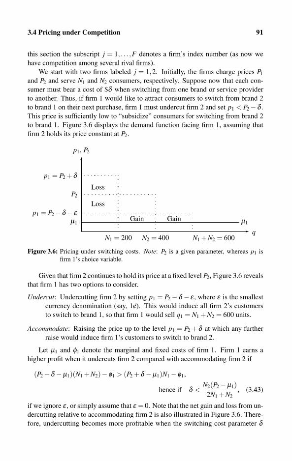
3.4 Pricing under Competition 91
this section the subscript j = 1, . . . ,F denotes a firm’s index number (as now we
have competition among several rival firms).
We start with two firms labeled j = 1,2. Initially, the firms charge prices P1
and P2 and serve N1 and N2 consumers, respectively. Suppose now that each con-
sumer must bear a cost of $δ when switching from one brand or service provider
to another. Thus, if firm 1 would like to attract consumers to switch from brand 2
to brand 1 on their next purchase, firm 1 must undercut firm 2 and set p1 < P2−δ .
This price is sufficiently low to “subsidize” consumers for switching from brand 2
to brand 1. Figure 3.6 displays the demand function facing firm 1, assuming that
firm 2 holds its price constant at P2.
�
�
q
p1, P2
N2 = 400N1 = 200 N1 +N2 = 600
P2
μ1 μ1
p1 = P2 +δ
p1 = P2−δ − ε
Loss
Loss
Gain Gain
Figure 3.6: Pricing under switching costs. Note: P2 is a given parameter, whereas p1 is
firm 1’s choice variable.
Given that firm 2 continues to hold its price at a fixed level P2, Figure 3.6 reveals
that firm 1 has two options to consider.
Undercut: Undercutting firm 2 by setting p1 = P2−δ − ε , where ε is the smallest
currency denomination (say, 1/c). This would induce all firm 2’s customers
to switch to brand 1, so that firm 1 would sell q1 = N1 +N2 = 600 units.
Accommodate: Raising the price up to the level p1 = P2 + δ at which any further
raise would induce firm 1’s customers to switch to brand 2.
Let μ1 and φ1 denote the marginal and fixed costs of firm 1. Firm 1 earns a
higher profit when it undercuts firm 2 compared with accommodating firm 2 if
(P2−δ −μ1)(N1 +N2)−φ1 > (P2 +δ −μ1)N1−φ1,
hence if δ <N2(P2−μ1)
2N1 +N2, (3.43)
if we ignore ε , or simply assume that ε = 0. Note that the net gain and loss from un-
dercutting relative to accommodating firm 2 is also illustrated in Figure 3.6. There-
fore, undercutting becomes more profitable when the switching cost parameter δ
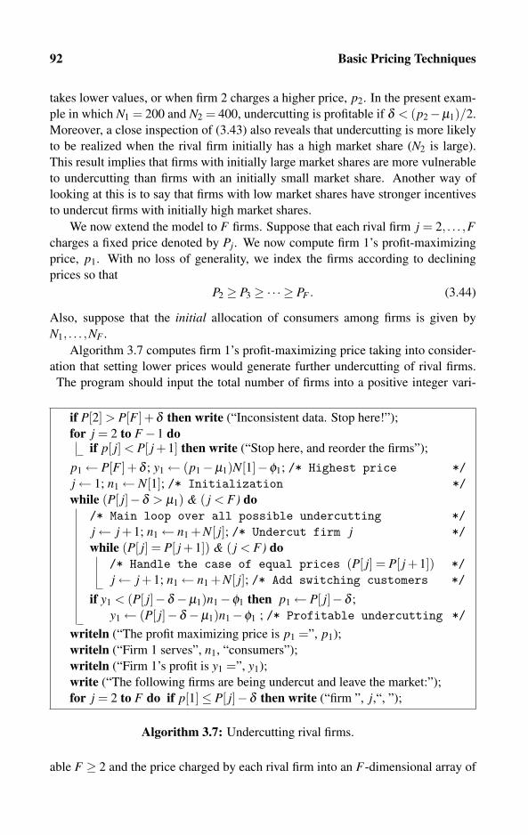
92 Basic Pricing Techniques
takes lower values, or when firm 2 charges a higher price, p2. In the present exam-
ple in which N1 = 200 and N2 = 400, undercutting is profitable if δ < (p2−μ1)/2.
Moreover, a close inspection of (3.43) also reveals that undercutting is more likely
to be realized when the rival firm initially has a high market share (N2 is large).
This result implies that firms with initially large market shares are more vulnerable
to undercutting than firms with an initially small market share. Another way of
looking at this is to say that firms with low market shares have stronger incentives
to undercut firms with initially high market shares.
We now extend the model to F firms. Suppose that each rival firm j = 2, . . . ,Fcharges a fixed price denoted by Pj. We now compute firm 1’s profit-maximizing
price, p1. With no loss of generality, we index the firms according to declining
prices so that
P2 ≥ P3 ≥ ·· · ≥ PF . (3.44)
Also, suppose that the initial allocation of consumers among firms is given by
N1, . . . ,NF .
Algorithm 3.7 computes firm 1’s profit-maximizing price taking into consider-
ation that setting lower prices would generate further undercutting of rival firms.
The program should input the total number of firms into a positive integer vari-
if P[2] > P[F ]+δ then write (“Inconsistent data. Stop here!”);
for j = 2 to F−1 doif p[ j] < P[ j +1] then write (“Stop here, and reorder the firms”);
p1← P[F ]+δ ; y1← (p1−μ1)N[1]−φ1; /* Highest price */j← 1; n1← N[1]; /* Initialization */while (P[ j]−δ > μ1) & ( j < F) do
/* Main loop over all possible undercutting */j← j +1; n1← n1 +N[ j]; /* Undercut firm j */while (P[ j] = P[ j +1]) & ( j < F) do
/* Handle the case of equal prices (P[ j] = P[ j +1]) */j← j +1; n1← n1 +N[ j]; /* Add switching customers */
if y1 < (P[ j]−δ −μ1)n1−φ1 then p1← P[ j]−δ ;
y1← (P[ j]−δ −μ1)n1−φ1 ; /* Profitable undercutting */
writeln (“The profit maximizing price is p1 =”, p1);
writeln (“Firm 1 serves”, n1, “consumers”);
writeln (“Firm 1’s profit is y1 =”, y1);
write (“The following firms are being undercut and leave the market:”);
for j = 2 to F do if p[1]≤ P[ j]−δ then write (“firm ”, j,“, ”);
Algorithm 3.7: Undercutting rival firms.
able F ≥ 2 and the price charged by each rival firm into an F-dimensional array of
3.4 Pricing under Competition 93
nonnegative real P[�], � = 2,3, . . . ,F . Note that p[1] need not be assigned an initial
value because it is the main choice variable of this algorithm, which is denoted by
p1. Finally, the program should input the switching cost parameter into a nonneg-
ative real parameter δ , as well as firm 1’s marginal and fixed cost parameters μ1
and φ1.
Algorithm 3.7 runs as follows: First, it verifies that the difference between
any two prices does not exceed the switching cost parameter δ . Clearly, if the
difference in prices exceeds the switching cost, the firm charging the higher price
cannot maintain any market share because all of its customers would switch to the
cheaper brand. Therefore, such a firm must be excluded from the present analysis.
Note that by our assumption regarding the way in which the firms are indexed given
in (3.44), it is sufficient to verify that p2− pF < δ . For this reason, Algorithm 3.7
also verifies that the firms are indexed according to (3.44).
Secondly, Algorithm 3.7 initially sets the highest possible price for firm 1
(p[1] = P[F ] + δ ) that is consistent with maintaining N[1] customers, and then
starts a “While” loop that gradually reduces the price, thereby undercutting more
and more firms. Therefore, there are F prices to experiment with, starting with
p1 = P[F ] + δ (keeping the initial N[1] consumers only), then reducing to p1 =P[2]− δ , thereby serving N[1] + N[2] consumers, and so on. During each loop,
the consumers from the firms being undercut are added to the integer-valued vari-
able n1, which measures firm 1’s sales, taking into account all the consumers who
switch to firm 1. This loop also compares the resulting profit and chooses the profit-
maximizing price. Finally, the second “While loop” is not needed if all rival firms
charge strictly different prices, that is, in the case in which (3.44) holds with strict
inequalities so that P[2] > P[3] > · · ·> P[F ].We now demonstrate how Algorithm 3.7 works for the case of F = 3 firms.
There are three values for p1 that should be compared. The first is no under-
cutting, in which case the maximum price that firm 1 can set is p1 = P[3] + δ .
The resulting profit is therefore y1 = (P[3] + δ − μ1)N[1]− φ1. The second pos-
sibility is to undercut firm 2 only by setting p1 = P[3]− δ , thereby earning y1 =(P[2]−δ−μ1)(N[1]+N[2])−φ1. Note, however, that if firms 2 and 3 charge equal
prices (P[2] = P[3]), then the “inner While loop” advances the index j to j = 3 and
computes the profit y1 = (P[3]−δ−μ)(N[1]+N[2]+N[3])−φ1, which is the profit
generated by undercutting firm 2 and firm 3 at the same time.
Retaliation of rival firms
Our analysis has so far relied on the assumption that only firm 1 is active, whereas
all other firms behave myopically in the sense that they don’t reduce their prices to
avoid being undercut by firm 1. Using a two-firm example, we now demonstrate
what would be the outcome if both firms 1 and 2 are free to choose their prices.
There could be several game-theoretic solutions for this type of problem. The
solution advocated by the author of this book is to use the so-called undercut-proof
94 Basic Pricing Techniques
equilibrium (see Shy 2001, 2002). The undercut-proof equilibrium is defined as
follows:
DEFINITION 3.1
For a given initial allocation of consumers between the firms, N1 and N2, the
undercut-proof equilibrium is the pair of prices (pU1 , pU
2 ) satisfying:
(a) For a given pU2 , firm 1 chooses the highest price pU
1 subject to
yU2 = (pU
2 −μ2)N2−φ2 ≥ (p1−δ −μ2)(N1 +N2)−φ2.
(b) For a given pU1 , firm 2 chooses the highest price pU
2 subject to
yU1 = (pU
1 −μ1)N1−φ1 ≥ (p2−δ −μ1)(N1 +N2)−φ1.
The first part states that, in an undercut-proof equilibrium, firm 1 sets the highest
price it can, but not too high as to prevent firm 2 from undercutting pU1 and grabbing
firm 1’s N1 customers. More precisely, firm 1 sets pU1 as high as possible, but not so
high that firm 2’s equilibrium profit level is not lower than firm 2’s profit level when
it undercuts firm 1 by setting p2 < pU1 −δ and sells to all the N1 +N2 consumers.
In equilibrium, the above two inequalities hold as equalities that can be solved
for the unique equilibrium prices
pU1 =
(N1)2(δ + μ2)+N1N2(3δ + μ2)(N2)2(2δ + μ1)(N1)2 +N1N2 +(N2)2
, (3.45)
pU2 =
(N1)2(2δ + μ2)+N1N2(3δ + μ1)+(N2)2(δ + μ1)(N1)2 +N1N2 +(N2)2
.
This solution to the undercut-proof equilibrium may generate negative prices, in
which case a solution may be found by looking for a price at which one firm can
undercut the other firm by leaving it with no customers and therefore with no profit.
We conclude this section on retaliation with a numerical example. Suppose
that the initial allocation of consumers is N1 = 200, N2 = 400, δ = $10, and firms’
marginal costs are μ1 = μ2 = $50. Substituting these values into the undercut-
proof equilibrium prices (3.45) obtains the undercut-proof equilibrium prices pU1 =
500/7 ≈ $71.42, and pU2 = 470/7 ≈ $67.14. Observe that in an undercut-proof
equilibrium (under equal marginal costs), the firm with the lower market share
charges a higher price, so pU1 > pU
2 . The interpretation of this result is that the
firm with the higher market share (firm 2 in the present example) has more to fear
from being undercut by the small firm, and to prevent this undercutting from being
profitable to its rival, it must maintain a lower market price.
The undercut-proof equilibrium derived in this section can be extended in two
ways. First, as in the next section, it can incorporate different quality brands, so that
consumers’ willingness to pay varies between the brands. Second, it can incorpo-
rate asymmetric switching costs rather easily by assuming that the cost of switching
from brand 1 to brand 2 is δ1,2 whereas the cost of switching from brand 2 to brand 1
is δ2,1, where the two switching costs need not be equal.
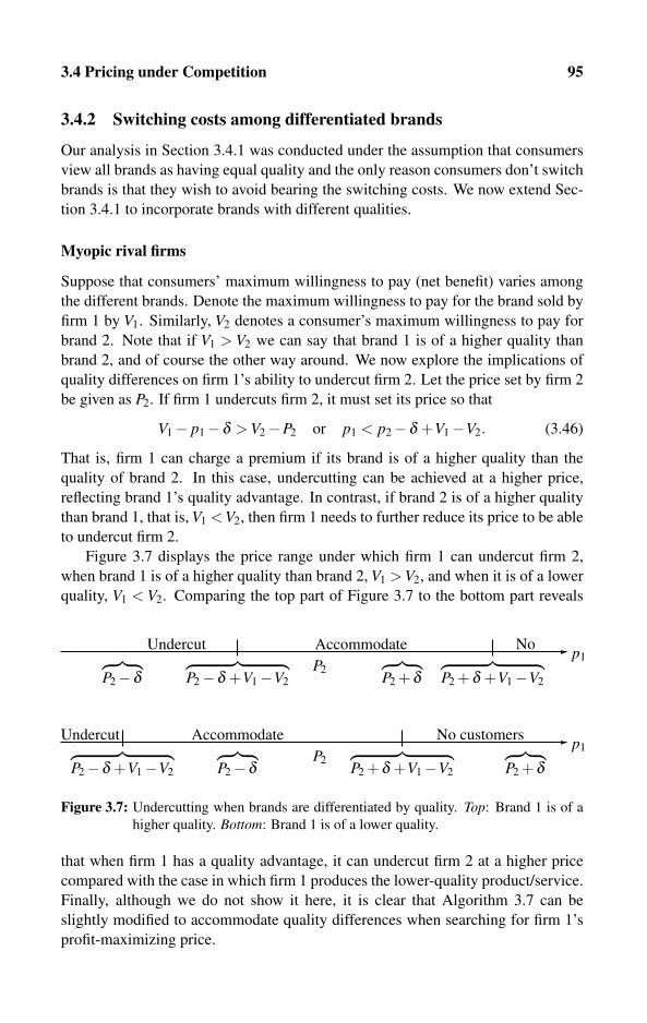
3.4 Pricing under Competition 95
3.4.2 Switching costs among differentiated brands
Our analysis in Section 3.4.1 was conducted under the assumption that consumers
view all brands as having equal quality and the only reason consumers don’t switch
brands is that they wish to avoid bearing the switching costs. We now extend Sec-
tion 3.4.1 to incorporate brands with different qualities.
Myopic rival firms
Suppose that consumers’ maximum willingness to pay (net benefit) varies among
the different brands. Denote the maximum willingness to pay for the brand sold by
firm 1 by V1. Similarly, V2 denotes a consumer’s maximum willingness to pay for
brand 2. Note that if V1 > V2 we can say that brand 1 is of a higher quality than
brand 2, and of course the other way around. We now explore the implications of
quality differences on firm 1’s ability to undercut firm 2. Let the price set by firm 2
be given as P2. If firm 1 undercuts firm 2, it must set its price so that
V1− p1−δ > V2−P2 or p1 < p2−δ +V1−V2. (3.46)
That is, firm 1 can charge a premium if its brand is of a higher quality than the
quality of brand 2. In this case, undercutting can be achieved at a higher price,
reflecting brand 1’s quality advantage. In contrast, if brand 2 is of a higher quality
than brand 1, that is, V1 < V2, then firm 1 needs to further reduce its price to be able
to undercut firm 2.
Figure 3.7 displays the price range under which firm 1 can undercut firm 2,
when brand 1 is of a higher quality than brand 2, V1 > V2, and when it is of a lower
quality, V1 < V2. Comparing the top part of Figure 3.7 to the bottom part reveals
� p1P2
︷ ︸︸ ︷P2 +δ +V1−V2
︷ ︸︸ ︷P2 +δ
︷ ︸︸ ︷P2−δ
No customersAccommodateUndercut︷ ︸︸ ︷P2−δ +V1−V2
� p1P2
︷ ︸︸ ︷P2 +δ
︷ ︸︸ ︷P2−δ +V1−V2
︷ ︸︸ ︷P2−δ
︷ ︸︸ ︷P2 +δ +V1−V2
Undercut Accommodate No
Figure 3.7: Undercutting when brands are differentiated by quality. Top: Brand 1 is of a
higher quality. Bottom: Brand 1 is of a lower quality.
that when firm 1 has a quality advantage, it can undercut firm 2 at a higher price
compared with the case in which firm 1 produces the lower-quality product/service.
Finally, although we do not show it here, it is clear that Algorithm 3.7 can be
slightly modified to accommodate quality differences when searching for firm 1’s
profit-maximizing price.

96 Basic Pricing Techniques
Retaliation by rival firms
Suppose now that firm 2 is allowed to retaliate, so p2 is no longer treated as constant
but as a strategic instrument set by firm 2. Under quality differences, Definition 3.1
should be modified as follows:
(p2−μ2)N2−φ2 ≥ (p1−δ +V2−V1−μ2)(N1 +N2)−φ2, (3.47)
(p1−μ1)N1−φ1 ≥ (p2−δ +V1−V2−μ1)(N1 +N2)−φ1.
That is, when firm 2 undercuts firm 1, it can add the quality difference V2−V1 to the
undercutting price to reflect its quality advantage or disadvantage. Similarly, when
firm 1 undercuts firm 2, it can add the quality difference V1−V2 to its undercutting
price.
Solving (3.47) for the equality case, the extension of (3.45) to brands differen-
tiated by quality is given by
pU1 =
(N1)2(V1−V2 +δ + μ2)+N1N2(V1−V2 +3δ + μ2)(N2)2(2δ + μ1)(N1)2 +N1N2 +(N2)2
,
(3.48)
pU2 =
(N1)2(2δ + μ2)+N1N2(V2−V1 +3δ + μ1)+(N2)2(V2−V1 +δ + μ1)(N1)2 +N1N2 +(N2)2
.
Clearly, substituting V1 = V2 into (3.48) obtains (3.45). Similar to the the basic
solution (3.45), the solution to the undercut-proof equilibrium for differentiated
brands (3.48) may also generate negative prices, in which case a solution may be
found by looking for a price at which one firm (perhaps the one producing the
higher quality) can undercut the other firm by leaving it with no customers, and
hence zero profit.
3.4.3 Continuous demand with differentiated brands
Section 2.7 analyzes continuous demand functions for differentiated brands, which
for the two-brand case, take the form of
q1(p1, p2)def= α1−β1 p1 + γ1 p2, (3.49)
q2(p1, p2)def= α2 + γ2 p1−β2 p2,
where β1 > 0 and β2 > 0 so that quantity demanded for each brand declines with
the brand’s own price. In addition, we must assume that β1 > |γ1| and β2 > |γ2|so that the “own-price effect” would always dominate the rival’s price effect. Def-
inition 2.4 has already established the general properties of the demand structure
given by (3.49) by classifying γ1 > 0 and γ2 > 0 as substitutes, and γ1 < 0 and
γ2 < 0 as complements.
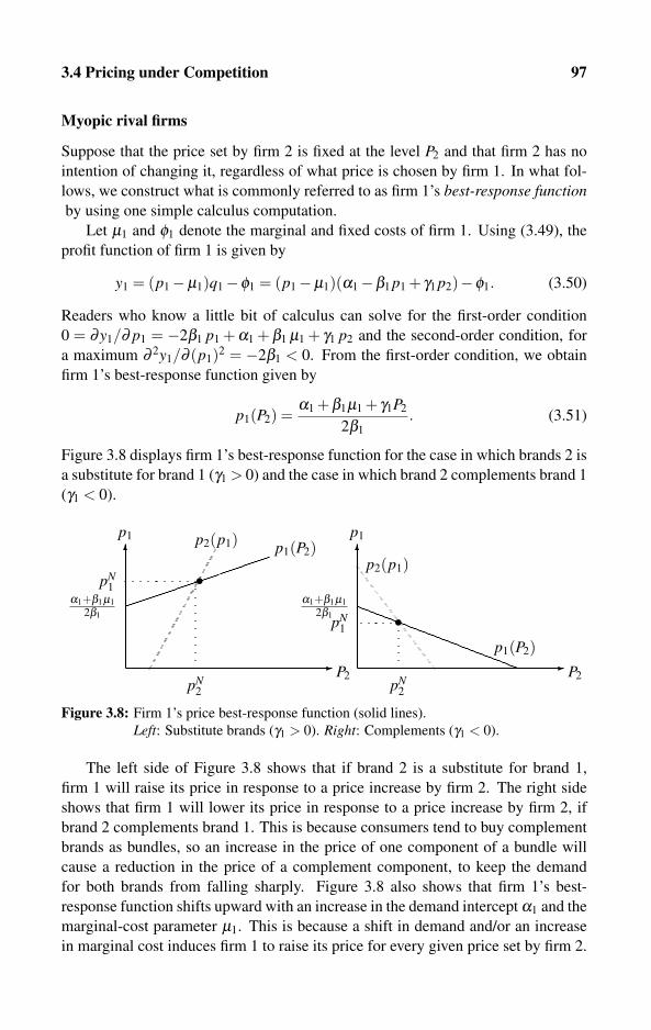
3.4 Pricing under Competition 97
Myopic rival firms
Suppose that the price set by firm 2 is fixed at the level P2 and that firm 2 has no
intention of changing it, regardless of what price is chosen by firm 1. In what fol-
lows, we construct what is commonly referred to as firm 1’s best-response functionby using one simple calculus computation.
Let μ1 and φ1 denote the marginal and fixed costs of firm 1. Using (3.49), the
profit function of firm 1 is given by
y1 = (p1−μ1)q1−φ1 = (p1−μ1)(α1−β1 p1 + γ1 p2)−φ1. (3.50)
Readers who know a little bit of calculus can solve for the first-order condition
0 = ∂y1/∂ p1 = −2β1 p1 + α1 + β1 μ1 + γ1 p2 and the second-order condition, for
a maximum ∂ 2y1/∂ (p1)2 = −2β1 < 0. From the first-order condition, we obtain
firm 1’s best-response function given by
p1(P2) =α1 +β1μ1 + γ1P2
2β1. (3.51)
Figure 3.8 displays firm 1’s best-response function for the case in which brands 2 is
a substitute for brand 1 (γ1 > 0) and the case in which brand 2 complements brand 1
(γ1 < 0).
�
�
P2
p1
α1+β1μ1
2β1
�
�
P2
p1
α1+β1μ1
2β1
p1(P2)
p1(P2)
p2(p1)
p2(p1)
pN1
pN2
pN1
pN2
•
•
Figure 3.8: Firm 1’s price best-response function (solid lines).
Left: Substitute brands (γ1 > 0). Right: Complements (γ1 < 0).
The left side of Figure 3.8 shows that if brand 2 is a substitute for brand 1,
firm 1 will raise its price in response to a price increase by firm 2. The right side
shows that firm 1 will lower its price in response to a price increase by firm 2, if
brand 2 complements brand 1. This is because consumers tend to buy complement
brands as bundles, so an increase in the price of one component of a bundle will
cause a reduction in the price of a complement component, to keep the demand
for both brands from falling sharply. Figure 3.8 also shows that firm 1’s best-
response function shifts upward with an increase in the demand intercept α1 and the
marginal-cost parameter μ1. This is because a shift in demand and/or an increase
in marginal cost induces firm 1 to raise its price for every given price set by firm 2.

98 Basic Pricing Techniques
Retaliation by rival firms
Now suppose that firm 2 can also adjust its price in response to price changes made
by firm 1. Let μ2 and φ2 denote the marginal and fixed costs of firm 2. Using (3.49),
the profit function of firm 2 is given by
y2 = (p2−μ2)q2−φ2 = (p2−μ2)(α2 + γ2 p1−β2 p2)−φ2. (3.52)
The first-order condition is given by 0 = ∂y2/∂ p2 =−2β2 p2 +α2 +β2 μ2 + γ2 p1,
and the second-order condition for a maximum is ∂ 2y2/∂ (p2)2 =−2β2 < 0. From
the first-order condition, we obtain firm 2’s best-response function, given by
p2(p1) =α2 +β2μ2 + γ2 p1
2β2. (3.53)
The best-response function (3.53) is drawn in Figure 3.8 using dashed lines. Note
that the axes are “flipped” for equation (3.53) in the sense that the dependent vari-
able p2 is plotted on the horizontal axis, whereas the independent variable p1 is on
the vertical axis.
The last step for computing p1 and p2 is to define an equilibrium concept that
would serve as a prediction for which prices are likely to be realized once firms stop
responding to price changes made by rival firms. We make the following definition:
DEFINITION 3.2
A pair of prices (pN1 , pN
2 ) is called a Nash-Bertrand equilibrium if pN1 is firm 1’s
best response to pN2 , and pN
2 is firm 2’s best response to pN1 .
In other words, the pair of prices must be on the best-response function of each
active firm. The Nash-Bertrand equilibrium pair of prices (pN1 , pN
2 ) is plotted in
Figure 3.8 as the intersection of the two best-response functions. To obtain a nu-
merical solution, solving (3.51) and (3.53) yields the equilibrium price pair
pN1 =
α2γ1 +β2(2α1 +2β1μ1 + γ1μ2)4β1β2− γ1γ2
, (3.54)
pN2 =
α1γ2 +β1(2α2 +2β2μ2 + γ2μ1)4β1β2− γ1γ2
. (3.55)
Extension to multiple firms
Consider a market for differentiated brands with F ≥ 2 firms, each producing a
different brand indexed by j = 1, . . . ,F . The aggregate consumer demand function
for each brand, given by (3.49) for the two-brand case, is now generalized to
q j(p1, . . . , pF) def= α j−β j p j +F
∑i=1i�= j
γ ij pi, j = 1, . . . ,F , (3.56)

3.5 Commonly Practiced Pricing Methods 99
where α j > 0, β j > 0. In addition, the “own-price effect” parameter must also
satisfy β j > ∑i�= j |γ ij|, so it is greater than the sum of all “cross-price effects.” Thus,
the demand for brand j is negatively related to p j, but is also affected by the prices
of all other brands pi for all brands i �= j, via the parameters γ ij. These parameters
can be estimated using the procedure described in Section 2.7 using time series
observations on prices of all existing brands.
Let μ j and φ j denote the marginal and fixed costs of each firm j, j = 1, . . . ,F .
Using (3.56), the profit function of a representative firm j is then given by
y j = (p j−μ j)q j−φ j = (p j−μ j)
⎛⎜⎝α j−β j p j +
F
∑i=1i�= j
γ ij pi
⎞⎟⎠−φ j. (3.57)
The first-order condition for a maximum is given by 0 = ∂y j/∂ p j =−2β j p j +α j +β j μ j +∑i�= j γ i
j pi, and the second-order condition for a maximum is ∂ 2y j/∂ (p j)2 =−2β j < 0. From the first-order condition, we obtain the best-response function for
each firm j, j = 1, . . . ,F ,
p j (pi | i �= j ) =
⎛⎜⎝α j +β j μ j +
F
∑i=1i�= j
γ ij pi
⎞⎟⎠/
(2β2). (3.58)
The best-response functions listed in (3.58) constitute a system of F linear equa-
tions that can be solved for the Nash-Bertrand equilibrium prices pN1 , . . . , pN
F , using
repeated substitution or some other method.
3.5 Commonly Practiced Pricing Methods
So far, our analysis in this chapter has been confined to the study of pricing tech-
niques by profit-maximizing firms (mostly monopolies), in which the presentation
reflected the standard economics approach. In reality, professional pricing practi-
tioners often use different terminology in specifying their pricing strategies.
3.5.1 Breakeven formulas
Breakeven formulas are commonly used by managers in charge of pricing policies
of their firms. Breakeven formulas provide the manager with some rough approx-
imations on how much output the firm should sell to break even. Some formulas
also indicate by how much sales should be increased to compensate for a price
reduction and leave the firm at the same level of profit that it earned before the
reduction in price.
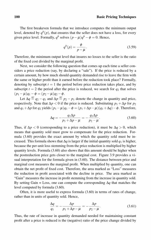
100 Basic Pricing Techniques
The first breakeven formula that we introduce computes the minimum output
level, denoted by qb(p), that ensures that the seller does not have a loss, for every
given price level. Formally, qb solves (p−μ)qb−φ = 0. Hence,
qb(p) =φ
p−μ. (3.59)
Therefore, the minimum output level that insures no losses to the seller is the ratio
of the fixed cost divided by the marginal profit.
Next, we consider the following question that comes up each time a seller con-
siders a price reduction (say, by declaring a “sale”). If the price is reduced by a
certain amount, by how much should quantity demanded rise to leave the firm with
the same or higher profit than it earned before the reduction took place? Formally,
denoting by subscript t = 1 the period before price reduction takes place, and by
subscript t = 2 the period after the price is reduced, we search for q2 that solves
(p1−μ)q1−φ = (p2−μ)q2−φ .
Let Δq def= q2− q1 and Δp def= p2− p1 denote the change in quantity and price,
respectively. Note that Δp < 0 if the price is reduced. Substituting p1 + Δp for p2
and q1 +Δp for q2 yields (p1−μ)q1−φ = (p1 +Δp−μ)(q1 +Δq)−φ . Therefore,
Δq =− q1Δpp1 +Δp−μ
=− q1Δpp2−μ
. (3.60)
Thus, if Δp < 0 (corresponding to a price reduction), it must be Δq > 0, which
means that quantity sold must grow to compensate for the price reduction. For-
mula (3.60) provides the exact amount by which the quantity sold must be in-
creased. This formula shows that Δq is larger if the initial quantity sold q1 is higher,
because the per-unit loss stemming from the price reduction is multiplied by higher
quantity levels. Formula (3.60) also shows that this amount should be higher when
the postreduction price gets closer to the marginal cost. Figure 3.9 provides a vi-
sual interpretation for the formula given in (3.60). The distance between price and
marginal cost measures the marginal profit. When multiplied by quantity, one can
obtain the net profit of fixed cost. Therefore, the area marked as “Loss” measures
the reduction in profit associated with the decline in price. The area marked as
“Gain” measures the increase in profit stemming from the increase in quantity sold.
By setting Gain = Loss, one can compute the corresponding Δq that matches the
level computed by formula (3.60).
Often, it is more useful to express formula (3.60) in terms of rates of change,
rather than in units of quantity sold. Hence,
Δqq1
=− Δpp1 +Δp−μ
=− Δpp2−μ
. (3.61)
Thus, the rate of increase in quantity demanded needed for maintaining constant
profit after a price is reduced is the (negative) ratio of the price change divided by
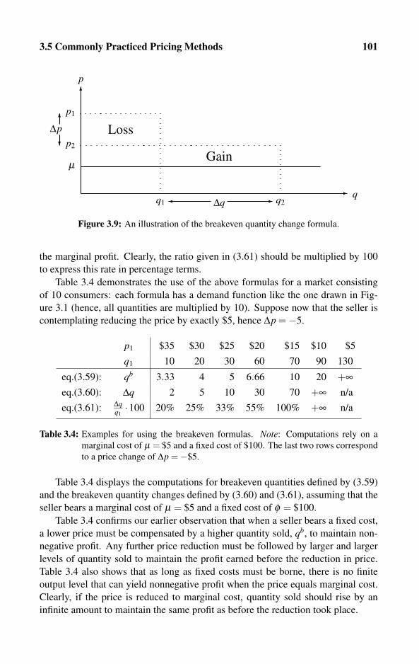
3.5 Commonly Practiced Pricing Methods 101
�
� q
p
μ
p1
q1 q2
p2
Loss
Gain
Δq ��
Δp�
Figure 3.9: An illustration of the breakeven quantity change formula.
the marginal profit. Clearly, the ratio given in (3.61) should be multiplied by 100
to express this rate in percentage terms.
Table 3.4 demonstrates the use of the above formulas for a market consisting
of 10 consumers: each formula has a demand function like the one drawn in Fig-
ure 3.1 (hence, all quantities are multiplied by 10). Suppose now that the seller is
contemplating reducing the price by exactly $5, hence Δp =−5.
p1 $35 $30 $25 $20 $15 $10 $5
q1 10 20 30 60 70 90 130
eq.(3.59): qb 3.33 4 5 6.66 10 20 +∞eq.(3.60): Δq 2 5 10 30 70 +∞ n/a
eq.(3.61): Δqq1·100 20% 25% 33% 55% 100% +∞ n/a
Table 3.4: Examples for using the breakeven formulas. Note: Computations rely on a
marginal cost of μ = $5 and a fixed cost of $100. The last two rows correspond
to a price change of Δp =−$5.
Table 3.4 displays the computations for breakeven quantities defined by (3.59)
and the breakeven quantity changes defined by (3.60) and (3.61), assuming that the
seller bears a marginal cost of μ = $5 and a fixed cost of φ = $100.
Table 3.4 confirms our earlier observation that when a seller bears a fixed cost,
a lower price must be compensated by a higher quantity sold, qb, to maintain non-
negative profit. Any further price reduction must be followed by larger and larger
levels of quantity sold to maintain the profit earned before the reduction in price.
Table 3.4 also shows that as long as fixed costs must be borne, there is no finite
output level that can yield nonnegative profit when the price equals marginal cost.
Clearly, if the price is reduced to marginal cost, quantity sold should rise by an
infinite amount to maintain the same profit as before the reduction took place.

102 Basic Pricing Techniques
3.5.2 Cost-plus pricing methods
Managers often tend to be risk averse in the sense that they select a price that
covers average total cost and perhaps add some markup above average total cost
to “ensure” nonnegative profits. Formally, managers often set a price consisting of
the following components:
p def= μ +φq
+up, (3.62)
where μ is the constant marginal-cost parameter, φ is the fixed cost, q is the output
produced (predicted sales level), and up is the desired markup. It should be empha-
sized that the markup up in (3.62) is a markup above all costs (marginal and fixed
costs!) as opposed to the ordinary definition of a markup, which is the difference
between price and marginal cost, p− μ . This particular definition of up is used
only in this section.
The pricing technique defined by (3.62) is called cost plus because it attempts
to secure the firm against a loss by imbedding marginal and fixed costs into the
price consumers pay. The term plus refers to the markup up, which may ensure
some strictly positive profit. Clearly, if the firm sets up = 0, the firm breaks even
because the price exactly equals the average total cost. The fixed cost component
is spread out over the q units that the firm sells to its customers. Thus, if the only
goal of the firm is to to break even, the manager can keep the price low by charging
a low markup, or even a zero markup. However, if the firm is a profit maximizer,
just like the firm we analyzed in earlier sections, the manager may want to compute
what should be the markup level that would correspond to the profit-maximizing
price.
Cost plus and linear demand
We now compute the markup level up that would generate the profit-maximizing
price. For the linear demand case, p = α−βq, we recall the solution to the “ordi-
nary” monopoly profit-maximization problem given in Section 3.1.2,
p =α + μ
2, q =
α−μ2β
, and y =(α−μ)2
4β−φ . (3.63)
Because we know that the profit level (3.63) is the “best” that the monopoly can
achieve, we now show how this profit level can be duplicated by a proper applica-
tion of the cost-plus method. To “properly” set the profit-maximizing markup up,
we equate (3.62) to the inverse demand function so that
p = α−βq = μ +φq
+up. (3.64)
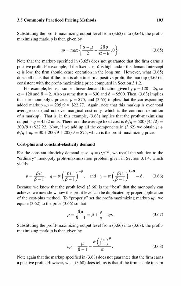
3.5 Commonly Practiced Pricing Methods 103
Substituting the profit-maximizing output level from (3.63) into (3.64), the profit-
maximizing markup is then given by
up = max
{α−μ
2− 2βφ
α−μ,0
}. (3.65)
Note that the markup specified in (3.65) does not guarantee that the firm earns a
positive profit. For example, if the fixed cost φ is high and/or the demand intercept
α is low, the firm should cease operation in the long run. However, what (3.65)
does tell us is that if the firm is able to earn a positive profit, the markup (3.65) is
consistent with the profit-maximizing price computed in Section 3.1.2.
For example, let us assume a linear demand function given by p = 120−2q, so
α = 120 and β = 2. Also assume that μ = $30 and φ = $500. Then, (3.63) implies
that the monopoly’s price is p = $75, and (3.65) implies that the corresponding
added markup up = 205/9 ≈ $22.77. Again, note that this markup is over total
average cost (and not over marginal cost only, which is the common definition
of a markup). That is, in this example, (3.63) implies that the profit-maximizing
output is q = 45/2 units. Therefore, the average fixed cost is φ/q = 500/(45/2) =200/9 ≈ $22.22. Now, if we add up all the components in (3.62) we obtain μ +φ/q+up = 30+200/9+205/9 = $75, which is the profit-maximizing price.
Cost-plus and constant-elasticity demand
For the constant-elasticity demand case, q = α p−β , we recall the solution to the
“ordinary” monopoly profit-maximization problem given in Section 3.1.4, which
yields
p =β μ
β −1, q = α
(β μ
β −1
)−β, and y = α
(β μ
β −1
)1−β−φ . (3.66)
Because we know that the profit level (3.66) is the “best” that the monopoly can
achieve, we now show how this profit level can be duplicated by proper application
of the cost-plus method. To “properly” set the profit-maximizing markup up, we
equate (3.62) to the price (3.66) so that
p =β μ
β −1= μ +
φq
+up. (3.67)
Substituting the profit-maximizing output level from (3.66) into (3.67), the profit-
maximizing markup is then given by
up =μ
β −1−
φ(
β μβ−1
)β
α. (3.68)
Note again that the markup specified in (3.68) does not guarantee that the firm earns
a positive profit. However, what (3.68) does tell us is that if the firm is able to earn

104 Basic Pricing Techniques
a positive profit, the markup (3.68) is consistent with the profit-maximizing price
computed in Section 3.1.4.
For example, let us assume that q = 72,000p−2, so α = 72,000 and β = 2. Also
assume that μ = $30 and that φ = $500. Then, (3.66) implies that the monopoly’s
price is p = $60, and (3.68) implies that the added markup (above average total
cost) up = $5. Equation (3.66) also implies that the monopoly’s output level is
q = 20. Hence, the average fixed cost is φ/q = 500/20 = $25. Now, if we add up
all the components in (3.62), we obtain μ +φ/q+up = 30+25+5 = $60, which
is the profit-maximizing price.
3.6 Regulated Public Utility
Regulators use different pricing methods as they take consumer welfare into con-
sideration in addition to firms’ profits. In this section, we analyze some of these
methods. Regulated firms are discussed in Section 5.5 in the context of two-part tar-
iffs, and in Section 6.7 in the context of peak-load pricing. Section 5.5, in particular,
contains some discussions on the objectives facing the regulator while deciding on
the socially optimal pricing structure.
3.6.1 Allocating fixed costs across markets while breaking even
The problem examined in this section is how to price markets characterized by
different demand functions given that the firm incurs a high fixed production cost
and given that the firm’s objective is to break even (as opposed to maximizing
profit). Note that Section 3.2 has already provided the general solution for the
profit-maximization problem with no price discrimination, and that Section 3.3 pro-
vided the same with price discrimination. These two sections clearly characterize
the profit-maximizing prices in the presence of common fixed costs, so no further
analysis is needed. For this reason, we now focus only on a firm that attempts to
break even.
There are several reasons why a firm’s objective would be to break even rather
than to maximize profit. First, some regulated public utilities and nonprofit organi-
zations operate precisely under the objective of breaking even. A full investigation
of public utilities is beyond the scope of this book. Readers who are interested
in regulated public utilities should consult several books, such as Crew and Klein-
dorfer (1979), Sharkey (1982), Brown and Sibley (1986), Sherman (1989), and
Viscusi, Vernon, and Harrington (1995). Also, for more recent books that ana-
lyze “regulated competition” (mainly in the telecommunications industry) readers
should consult Mitchell and Vogelsang (1991) and Laffont and Tirole (2001). A
second reason why the firm may want to break even (instead of maximizing profit)
is that a firm may be a subdivision or a unit of a larger conglomerate that supplies

3.6 Regulated Public Utility 105
parts or other services to its headquarters. In this case, the goal of this subdivi-
sion would be merely to ensure that it does not incur any loss while maintaining an
efficient production pattern.
Because in this section we do not consider profit maximization as the objective
of the firm, one should define an alternative objective according to which prices
are selected. The most commonly used objective used by regulators is to maximize
social welfare subject to ensuring that the seller or service provider breaks even.
However, because this book rarely addresses issues of social welfare, we will be
investigating some alternative objectives that vary by the restrictions imposed on
the firm in question. Therefore, we begin by first imposing a restriction on the
seller to charge equal prices in all markets, so all consumers must equally “share”
the fixed cost incurred by this firm. Then, we conclude by showing why “equal
sharing” of the firm’s fixed cost is inefficient according to a certain criterion.
Two markets with a uniform fee: An example
Consider a single firm serving two markets with the linear demand functions given
by
p1 = 80−q1 and p2 = 60−2q2, or q1 = 80− p1 and q2 =60− p2
2. (3.69)
The firm bears a constant marginal cost of μ = $40 and a fixed cost of φ = $350.
The regulator of this firm requires that (a) the firm break even so that total revenue
exactly equal total cost and (b) there is a uniform charge; that is, all the consumers
(or actually all units sold) are equally priced, and hence the fixed cost φ is equally
imbedded into the price of this service/product.
Formally, the firm is allowed to set a surcharge fee f , which must be uniform
across markets; the sole purpose of this fee is to pay for the fixed cost of φ = $350
incurred by this firm. By imbedding this fee (surcharge) into the price, the price
can be written as
p = μ + f = $40+ f , where f ·q1 + f ·q2 = φ = $350. (3.70)
The first part states that the “breakeven” price equals the sum of the marginal cost
and the fee, and the second part states that the proceeds from this per-unit fee, which
is levied equally in both markets, must exactly cover the fixed cost φ = $350.
We now demonstrate how to compute the fee f satisfying (3.70). Substituting
the direct demand functions (3.69) into (3.70) yields
f (80−40− f )+ f60−40− f
2= 350, hence f = $10. (3.71)
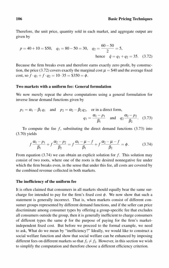
106 Basic Pricing Techniques
Therefore, the unit price, quantity sold in each market, and aggregate output are
given by
p = 40+10 = $50, q1 = 80−50 = 30, q2 =60−50
2= 5,
hence q = q1 +q2 = 35. (3.72)
Because the firm breaks even and therefore earns exactly zero profit, by construc-
tion, the price (3.72) covers exactly the marginal cost μ = $40 and the average fixed
cost, so f ·q1 + f ·q2 = 10 ·35 = $350 = φ .
Two markets with a uniform fee: General formulation
We now merely repeat the above computations using a general formulation for
inverse linear demand functions given by
p1 = α1−β1 q1 and p2 = α2−β2 q2, or in a direct form,
q1 =α1− p1
β1and q2
α2− p2
β2. (3.73)
To compute the fee f , substituting the direct demand functions (3.73) into
(3.70) yields
fα1− p1
β1+ f
α2− p2
β2= f
α1−μ− fβ1
+ fα2−μ− f
β2= φ . (3.74)
From equation (3.74) we can obtain an explicit solution for f . This solution may
consist of two roots, where one of the roots is the desired nonnegative fee under
which the firm breaks even, in the sense that under this fee, all costs are covered by
the combined revenue collected in both markets.
The inefficiency of the uniform fee
It is often claimed that consumers in all markets should equally bear the same sur-
charge fee intended to pay for the firm’s fixed cost φ . We now show that such a
statement is generally incorrect. That is, when markets consist of different con-
sumer groups represented by different demand functions, and if the seller can price
discriminate among consumer types by offering a group-specific fee that excludes
all consumers outside the group, then it is generally inefficient to charge consumers
of different types the same φ for the purpose of paying for the firm’s market-
independent fixed cost. But before we proceed to the formal example, we need
to ask, What do we mean by “inefficiency?” Ideally, we would like to construct a
social welfare function and show that social welfare can be enhanced by imposing
different fees on different markets so that f1 �= f2. However, in this section we wish
to simplify the computation and therefore choose a different efficiency criterion.
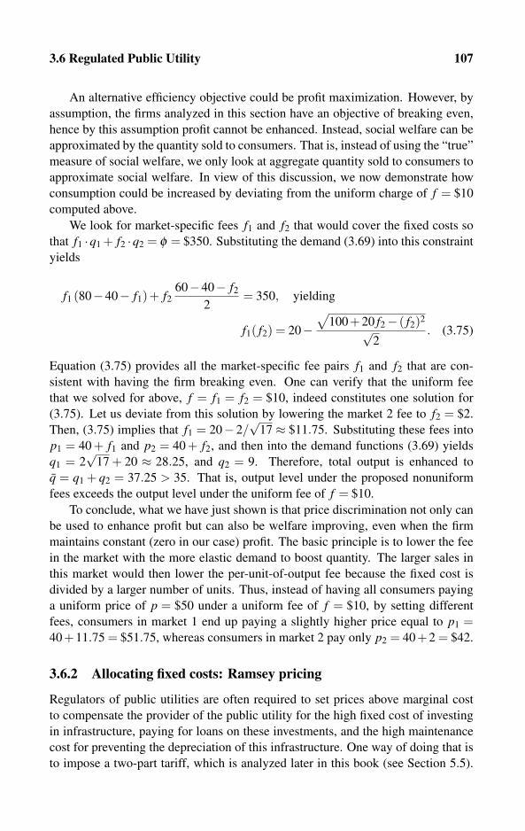
3.6 Regulated Public Utility 107
An alternative efficiency objective could be profit maximization. However, by
assumption, the firms analyzed in this section have an objective of breaking even,
hence by this assumption profit cannot be enhanced. Instead, social welfare can be
approximated by the quantity sold to consumers. That is, instead of using the “true”
measure of social welfare, we only look at aggregate quantity sold to consumers to
approximate social welfare. In view of this discussion, we now demonstrate how
consumption could be increased by deviating from the uniform charge of f = $10
computed above.
We look for market-specific fees f1 and f2 that would cover the fixed costs so
that f1 ·q1 + f2 ·q2 = φ = $350. Substituting the demand (3.69) into this constraint
yields
f1 (80−40− f1)+ f260−40− f2
2= 350, yielding
f1( f2) = 20−√
100+20 f2− ( f2)2
√2
. (3.75)
Equation (3.75) provides all the market-specific fee pairs f1 and f2 that are con-
sistent with having the firm breaking even. One can verify that the uniform fee
that we solved for above, f = f1 = f2 = $10, indeed constitutes one solution for
(3.75). Let us deviate from this solution by lowering the market 2 fee to f2 = $2.
Then, (3.75) implies that f1 = 20− 2/√
17 ≈ $11.75. Substituting these fees into
p1 = 40 + f1 and p2 = 40 + f2, and then into the demand functions (3.69) yields
q1 = 2√
17 + 20 ≈ 28.25, and q2 = 9. Therefore, total output is enhanced to
q = q1 + q2 = 37.25 > 35. That is, output level under the proposed nonuniform
fees exceeds the output level under the uniform fee of f = $10.
To conclude, what we have just shown is that price discrimination not only can
be used to enhance profit but can also be welfare improving, even when the firm
maintains constant (zero in our case) profit. The basic principle is to lower the fee
in the market with the more elastic demand to boost quantity. The larger sales in
this market would then lower the per-unit-of-output fee because the fixed cost is
divided by a larger number of units. Thus, instead of having all consumers paying
a uniform price of p = $50 under a uniform fee of f = $10, by setting different
fees, consumers in market 1 end up paying a slightly higher price equal to p1 =40+11.75 = $51.75, whereas consumers in market 2 pay only p2 = 40+2 = $42.
3.6.2 Allocating fixed costs: Ramsey pricing
Regulators of public utilities are often required to set prices above marginal cost
to compensate the provider of the public utility for the high fixed cost of investing
in infrastructure, paying for loans on these investments, and the high maintenance
cost for preventing the depreciation of this infrastructure. One way of doing that is
to impose a two-part tariff, which is analyzed later in this book (see Section 5.5).
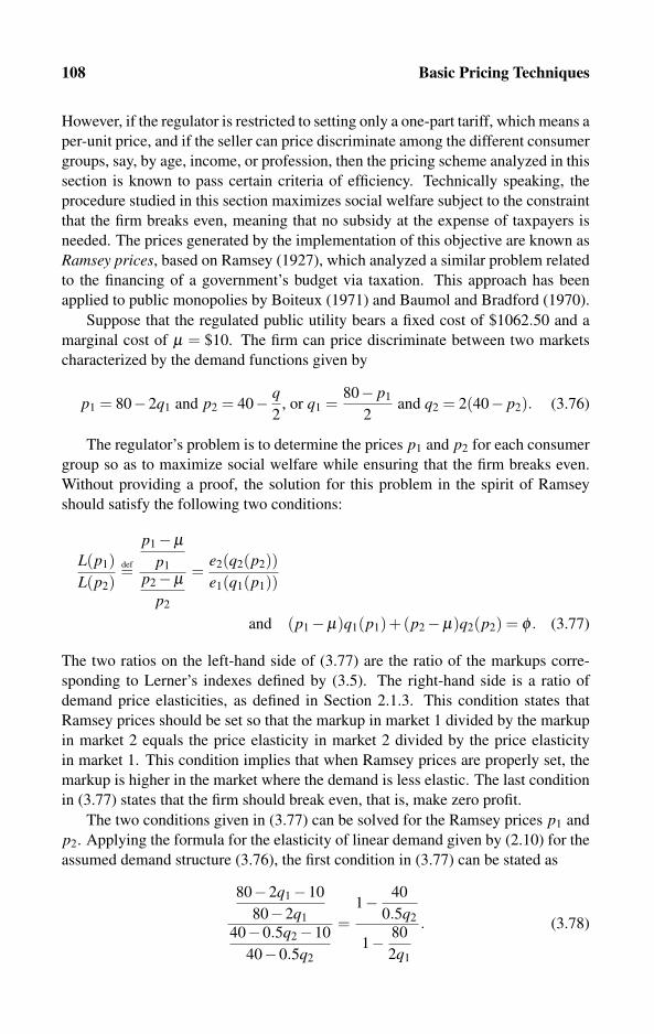
108 Basic Pricing Techniques
However, if the regulator is restricted to setting only a one-part tariff, which means a
per-unit price, and if the seller can price discriminate among the different consumer
groups, say, by age, income, or profession, then the pricing scheme analyzed in this
section is known to pass certain criteria of efficiency. Technically speaking, the
procedure studied in this section maximizes social welfare subject to the constraint
that the firm breaks even, meaning that no subsidy at the expense of taxpayers is
needed. The prices generated by the implementation of this objective are known as
Ramsey prices, based on Ramsey (1927), which analyzed a similar problem related
to the financing of a government’s budget via taxation. This approach has been
applied to public monopolies by Boiteux (1971) and Baumol and Bradford (1970).
Suppose that the regulated public utility bears a fixed cost of $1062.50 and a
marginal cost of μ = $10. The firm can price discriminate between two markets
characterized by the demand functions given by
p1 = 80−2q1 and p2 = 40− q2
, or q1 =80− p1
2and q2 = 2(40− p2). (3.76)
The regulator’s problem is to determine the prices p1 and p2 for each consumer
group so as to maximize social welfare while ensuring that the firm breaks even.
Without providing a proof, the solution for this problem in the spirit of Ramsey
should satisfy the following two conditions:
L(p1)L(p2)
def=
p1−μp1
p2−μp2
=e2(q2(p2))e1(q1(p1))
and (p1−μ)q1(p1)+(p2−μ)q2(p2) = φ . (3.77)
The two ratios on the left-hand side of (3.77) are the ratio of the markups corre-
sponding to Lerner’s indexes defined by (3.5). The right-hand side is a ratio of
demand price elasticities, as defined in Section 2.1.3. This condition states that
Ramsey prices should be set so that the markup in market 1 divided by the markup
in market 2 equals the price elasticity in market 2 divided by the price elasticity
in market 1. This condition implies that when Ramsey prices are properly set, the
markup is higher in the market where the demand is less elastic. The last condition
in (3.77) states that the firm should break even, that is, make zero profit.
The two conditions given in (3.77) can be solved for the Ramsey prices p1 and
p2. Applying the formula for the elasticity of linear demand given by (2.10) for the
assumed demand structure (3.76), the first condition in (3.77) can be stated as
80−2q1−10
80−2q1
40−0.5q2−10
40−0.5q2
=1− 40
0.5q2
1− 80
2q1
. (3.78)

3.6 Regulated Public Utility 109
Also, the first (breakeven) condition in (3.77) is given by
(p1−10)q1 +(p2−10)q2 = (80−2q1−10)q1 +(40− q2
2−10)q2 = 625. (3.79)
Solving (3.78) yields q1 = 7q2/12. Substituting this for q1 in (3.79) yields qR2 = 30.
Therefore,
qR1 = 17.5 and qR
2 = 30, hence pR1 (17.5) = $45 and pR
2 (30) = $25. (3.80)
Figure 3.10 illustrates the Ramsey prices and how they relate to price elasticities in
the two markets. Using the formula given by (2.10), the price elasticities in these
markets are given by
e1(17.5) = 1− α1
β1 ·17.5=
9
7≈−1.28, and
e2(30) = 1− α2
β2 ·30=
5
3≈−1.66. (3.81)
�
�
����������������������������
��
��
���
q1, q2
p1, p2
40 80
$40
$20
$80
0 60
$60
p1 = 80−2q1
$10 μ
3010 17.5
$25
$45
p2 = 40− q2
2
�
�
e1(17.5)≈−1.28
e2(30)≈−1.66•
•
Figure 3.10: An illustration of Ramsey prices.
Thus, as illustrated in Figure 3.10, the markup in market 1 (with the less elastic
demand, |e1(20 = 1.28|) is higher than in market 2 (with the more elastic demand,
|e2(20 = 1.66|).
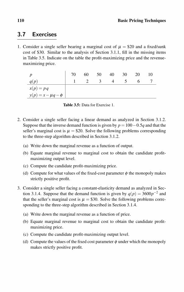
110 Basic Pricing Techniques
3.7 Exercises
1. Consider a single seller bearing a marginal cost of μ = $20 and a fixed/sunk
cost of $30. Similar to the analysis of Section 3.1.1, fill in the missing items
in Table 3.5. Indicate on the table the profit-maximizing price and the revenue-
maximizing price.
p 70 60 50 40 30 20 10
q(p) 1 2 3 4 5 6 7
x(p) = pq
y(p) = x−μq−φ
Table 3.5: Data for Exercise 1.
2. Consider a single seller facing a linear demand as analyzed in Section 3.1.2.
Suppose that the inverse demand function is given by p = 100−0.5q and that the
seller’s marginal cost is μ = $20. Solve the following problems corresponding
to the three-step algorithm described in Section 3.1.2.
(a) Write down the marginal revenue as a function of output.
(b) Equate marginal revenue to marginal cost to obtain the candidate profit-
maximizing output level.
(c) Compute the candidate profit-maximizing price.
(d) Compute for what values of the fixed-cost parameter φ the monopoly makes
strictly positive profit.
3. Consider a single seller facing a constant-elasticity demand as analyzed in Sec-
tion 3.1.4. Suppose that the demand function is given by q(p) = 3600p−2 and
that the seller’s marginal cost is μ = $30. Solve the following problems corre-
sponding to the three-step algorithm described in Section 3.1.4.
(a) Write down the marginal revenue as a function of price.
(b) Equate marginal revenue to marginal cost to obtain the candidate profit-
maximizing price.
(c) Compute the candidate profit-maximizing output level.
(d) Compute the values of the fixed cost parameter φ under which the monopoly
makes strictly positive profit.
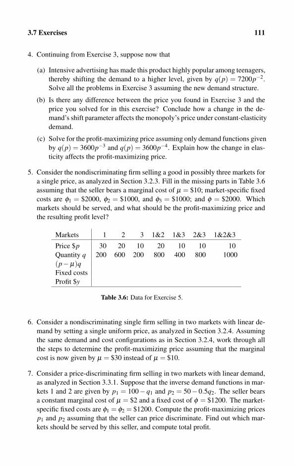
3.7 Exercises 111
4. Continuing from Exercise 3, suppose now that
(a) Intensive advertising has made this product highly popular among teenagers,
thereby shifting the demand to a higher level, given by q(p) = 7200p−2.
Solve all the problems in Exercise 3 assuming the new demand structure.
(b) Is there any difference between the price you found in Exercise 3 and the
price you solved for in this exercise? Conclude how a change in the de-
mand’s shift parameter affects the monopoly’s price under constant-elasticity
demand.
(c) Solve for the profit-maximizing price assuming only demand functions given
by q(p) = 3600p−3 and q(p) = 3600p−4. Explain how the change in elas-
ticity affects the profit-maximizing price.
5. Consider the nondiscriminating firm selling a good in possibly three markets for
a single price, as analyzed in Section 3.2.3. Fill in the missing parts in Table 3.6
assuming that the seller bears a marginal cost of μ = $10; market-specific fixed
costs are φ1 = $2000, φ2 = $1000, and φ3 = $1000; and φ = $2000. Which
markets should be served, and what should be the profit-maximizing price and
the resulting profit level?
Markets 1 2 3 1&2 1&3 2&3 1&2&3
Price $p 30 20 10 20 10 10 10
Quantity q 200 600 200 800 400 800 1000
(p−μ)qFixed costs
Profit $y
Table 3.6: Data for Exercise 5.
6. Consider a nondiscriminating single firm selling in two markets with linear de-
mand by setting a single uniform price, as analyzed in Section 3.2.4. Assuming
the same demand and cost configurations as in Section 3.2.4, work through all
the steps to determine the profit-maximizing price assuming that the marginal
cost is now given by μ = $30 instead of μ = $10.
7. Consider a price-discriminating firm selling in two markets with linear demand,
as analyzed in Section 3.3.1. Suppose that the inverse demand functions in mar-
kets 1 and 2 are given by p1 = 100− q1 and p2 = 50−0.5q2. The seller bears
a constant marginal cost of μ = $2 and a fixed cost of φ = $1200. The market-
specific fixed costs are φ1 = φ2 = $1200. Compute the profit-maximizing prices
p1 and p2 assuming that the seller can price discriminate. Find out which mar-
kets should be served by this seller, and compute total profit.
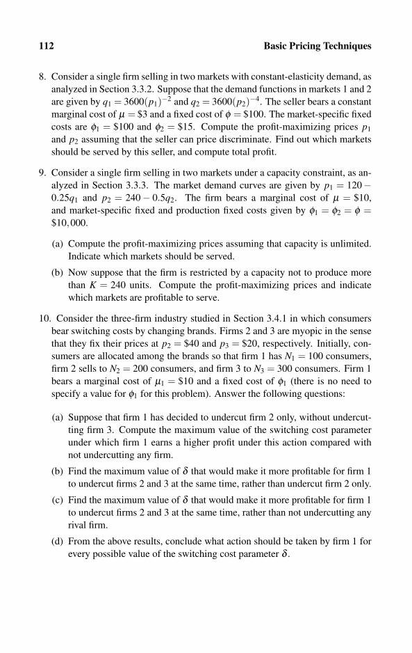
112 Basic Pricing Techniques
8. Consider a single firm selling in two markets with constant-elasticity demand, as
analyzed in Section 3.3.2. Suppose that the demand functions in markets 1 and 2
are given by q1 = 3600(p1)−2 and q2 = 3600(p2)−4. The seller bears a constant
marginal cost of μ = $3 and a fixed cost of φ = $100. The market-specific fixed
costs are φ1 = $100 and φ2 = $15. Compute the profit-maximizing prices p1
and p2 assuming that the seller can price discriminate. Find out which markets
should be served by this seller, and compute total profit.
9. Consider a single firm selling in two markets under a capacity constraint, as an-
alyzed in Section 3.3.3. The market demand curves are given by p1 = 120−0.25q1 and p2 = 240− 0.5q2. The firm bears a marginal cost of μ = $10,
and market-specific fixed and production fixed costs given by φ1 = φ2 = φ =$10,000.
(a) Compute the profit-maximizing prices assuming that capacity is unlimited.
Indicate which markets should be served.
(b) Now suppose that the firm is restricted by a capacity not to produce more
than K = 240 units. Compute the profit-maximizing prices and indicate
which markets are profitable to serve.
10. Consider the three-firm industry studied in Section 3.4.1 in which consumers
bear switching costs by changing brands. Firms 2 and 3 are myopic in the sense
that they fix their prices at p2 = $40 and p3 = $20, respectively. Initially, con-
sumers are allocated among the brands so that firm 1 has N1 = 100 consumers,
firm 2 sells to N2 = 200 consumers, and firm 3 to N3 = 300 consumers. Firm 1
bears a marginal cost of μ1 = $10 and a fixed cost of φ1 (there is no need to
specify a value for φ1 for this problem). Answer the following questions:
(a) Suppose that firm 1 has decided to undercut firm 2 only, without undercut-
ting firm 3. Compute the maximum value of the switching cost parameter
under which firm 1 earns a higher profit under this action compared with
not undercutting any firm.
(b) Find the maximum value of δ that would make it more profitable for firm 1
to undercut firms 2 and 3 at the same time, rather than undercut firm 2 only.
(c) Find the maximum value of δ that would make it more profitable for firm 1
to undercut firms 2 and 3 at the same time, rather than not undercutting any
rival firm.
(d) From the above results, conclude what action should be taken by firm 1 for
every possible value of the switching cost parameter δ .
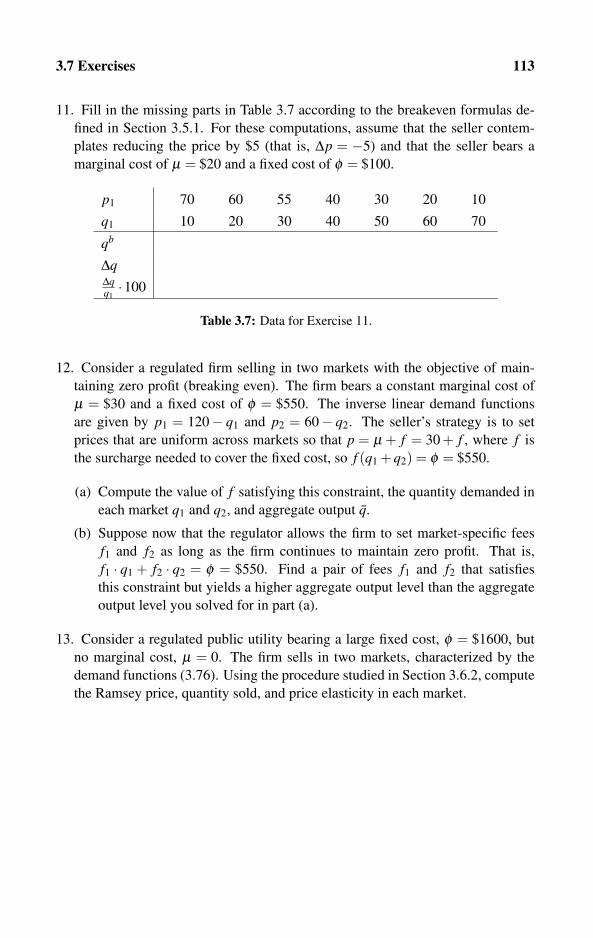
3.7 Exercises 113
11. Fill in the missing parts in Table 3.7 according to the breakeven formulas de-
fined in Section 3.5.1. For these computations, assume that the seller contem-
plates reducing the price by $5 (that is, Δp = −5) and that the seller bears a
marginal cost of μ = $20 and a fixed cost of φ = $100.
p1 70 60 55 40 30 20 10
q1 10 20 30 40 50 60 70
qb
ΔqΔqq1·100
Table 3.7: Data for Exercise 11.
12. Consider a regulated firm selling in two markets with the objective of main-
taining zero profit (breaking even). The firm bears a constant marginal cost of
μ = $30 and a fixed cost of φ = $550. The inverse linear demand functions
are given by p1 = 120− q1 and p2 = 60− q2. The seller’s strategy is to set
prices that are uniform across markets so that p = μ + f = 30 + f , where f is
the surcharge needed to cover the fixed cost, so f (q1 +q2) = φ = $550.
(a) Compute the value of f satisfying this constraint, the quantity demanded in
each market q1 and q2, and aggregate output q.
(b) Suppose now that the regulator allows the firm to set market-specific fees
f1 and f2 as long as the firm continues to maintain zero profit. That is,
f1 · q1 + f2 · q2 = φ = $550. Find a pair of fees f1 and f2 that satisfies
this constraint but yields a higher aggregate output level than the aggregate
output level you solved for in part (a).
13. Consider a regulated public utility bearing a large fixed cost, φ = $1600, but
no marginal cost, μ = 0. The firm sells in two markets, characterized by the
demand functions (3.76). Using the procedure studied in Section 3.6.2, compute
the Ramsey price, quantity sold, and price elasticity in each market.


Chapter 4
Bundling and Tying
4.1 Bundling 1174.1.1 Single-package bundling with identical consumers
4.1.2 Single-package bundling with two consumer types
4.1.3 A computer algorithm for multiple types
4.1.4 Multi-package bundling
4.2 Tying 1314.2.1 Pure tying: Theory and examples
4.2.2 Pure tying versus no tying: Computer algorithms
4.2.3 Mixed tying
4.2.4 Multi-package tying
4.3 Exercises 145
Bundling and tying are widely used instruments for implementing price discrim-
ination. Market segmentation is therefore accomplished by offering consumers a
variety of packages to choose from. When bundling is used, by choosing different
packages, consumers implicity reveal their willingness to pay for different quantity
levels of the same good. That is, consumers with a high preference for large quan-
tities will choose large bundles, whereas consumers with a low preference for large
quantities will choose small bundles, or simply buy one unit, if available. Simi-
larly, when tying is used, consumers implicitly reveal their preferences for some
other types of goods, which are tied to the sale of the original good. Both the
bundling and tying pricing techniques constitute special cases of nonlinear pric-
ing under which the price of each unit may vary with the total number of units
purchased.
The terms bundling and tying are used interchangeably both in the academic
literature and by pricing experts. In this book, however, we draw a sharp distinc-
tion between these two marketing instruments. We will be using the following
terminology:

116 Bundling and Tying
DEFINITION 4.1
(a) We say that a seller practices bundling if the firm sells packages containing at
least two units of the same product or service.
(b) We say that a seller practices tying if the firm sells packages containing at least
two different products or services.
Basically, the easiest way to remember the distinction made by Definition 4.1 is to
associate bundling with the sale of different quantities of the same good, whereas
tying refers to the sale of different (related or unrelated) goods that are “packed”
into a single package. Bundling is widely observed in large warehouses where the
seller, for example, tapes five packages of toothpaste together and prices the entire
package instead of each unit separately. The practice of bundling often takes the
form of subscriptions, for example, by selling a ticket for 10 health club visits or
10 entries to a swimming pool, and a wide variety transportation passes, such as
daily, weekly, monthly, or yearly passes that allow the holders of these passes to
take unlimited rides on public transportation such as buses and subways.
In some cases it is difficult to distinguish between bundling and tying. For ex-
ample, when a movie theater sells a ticket for 10 shows, the bundling interpretation
would regard it as selling 10 movies for an average price less than the price of a
single feature. However, if the variety of movies is limited, one may regard this
action as as attempt to sell the less-popular movies together with the more popular
ones, thereby increasing the demand for “bad” movies.
Our analysis in this chapter is self-contained and does not follow any particular
paper from the scientific literature. Most of the literature in economics journals is
about tying (although following our earlier discussion, the term bundling is used
in place of tying). We will not review this literature here. Instead, we list a few
important papers on this topic. Burstein (1960) provides an early analysis of tying.
Adams and Yellen (1976) introduce a graphical analysis of consumer choice un-
der tying. Other literature includes Schmalensee (1982, 1984), Dansby and Cecilia
(1984), Lewbel (1985), Pierce and Winter (1996), and Venkatesh and Kamakura
(2003). Literature that deviates from the monopoly market structure includes An-
derson and Leruth (1993), Pierce and Winter (1996), Chen (1997a), Liao and Tau-
man (2002), and Vaubourg (2006).
Several analytical papers, such as McAfee, McMillan, and Whinston (1989);
Carbajo, de Meza, and Seidmann (1990); Whinston (1990); Seidmann (1991); and
Horn and Shy (1996), tackle the issue of leveraging associated with tied sales, in
which the question analyzed is whether a monopoly in one market can enhance its
monopoly in another market by tying the sale of the two goods in the two different
markets. This line of research went even further by investigating whether the tying
firm can foreclose on its rivals in competing markets. This problem may arise in
particular in newly regulated telecommunications markets where, for example, a
local provider of telephone services can tie in the sale of Internet services to drive
competing Internet providers out of this market. Nalebuff (2004) investigated a
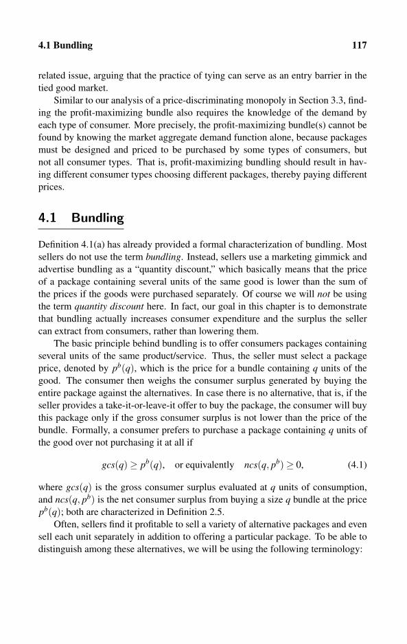
4.1 Bundling 117
related issue, arguing that the practice of tying can serve as an entry barrier in the
tied good market.
Similar to our analysis of a price-discriminating monopoly in Section 3.3, find-
ing the profit-maximizing bundle also requires the knowledge of the demand by
each type of consumer. More precisely, the profit-maximizing bundle(s) cannot be
found by knowing the market aggregate demand function alone, because packages
must be designed and priced to be purchased by some types of consumers, but
not all consumer types. That is, profit-maximizing bundling should result in hav-
ing different consumer types choosing different packages, thereby paying different
prices.
4.1 Bundling
Definition 4.1(a) has already provided a formal characterization of bundling. Most
sellers do not use the term bundling. Instead, sellers use a marketing gimmick and
advertise bundling as a “quantity discount,” which basically means that the price
of a package containing several units of the same good is lower than the sum of
the prices if the goods were purchased separately. Of course we will not be using
the term quantity discount here. In fact, our goal in this chapter is to demonstrate
that bundling actually increases consumer expenditure and the surplus the seller
can extract from consumers, rather than lowering them.
The basic principle behind bundling is to offer consumers packages containing
several units of the same product/service. Thus, the seller must select a package
price, denoted by pb(q), which is the price for a bundle containing q units of the
good. The consumer then weighs the consumer surplus generated by buying the
entire package against the alternatives. In case there is no alternative, that is, if the
seller provides a take-it-or-leave-it offer to buy the package, the consumer will buy
this package only if the gross consumer surplus is not lower than the price of the
bundle. Formally, a consumer prefers to purchase a package containing q units of
the good over not purchasing it at all if
gcs(q)≥ pb(q), or equivalently ncs(q, pb)≥ 0, (4.1)
where gcs(q) is the gross consumer surplus evaluated at q units of consumption,
and ncs(q, pb) is the net consumer surplus from buying a size q bundle at the price
pb(q); both are characterized in Definition 2.5.
Often, sellers find it profitable to sell a variety of alternative packages and even
sell each unit separately in addition to offering a particular package. To be able to
distinguish among these alternatives, we will be using the following terminology:
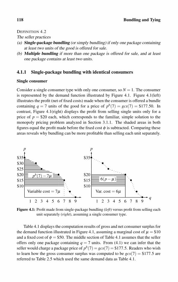
118 Bundling and Tying
DEFINITION 4.2
The seller practices
(a) Single-package bundling (or simply bundling) if only one package containing
at least two units of the good is offered for sale.
(b) Multiple bundling if more than one package is offered for sale, and at least
one package contains at least two units.
4.1.1 Single-package bundling with identical consumers
Single consumer
Consider a single consumer type with only one consumer, so N = 1. The consumer
is represented by the demand function illustrated by Figure 4.1. Figure 4.1(left)
illustrates the profit (net of fixed costs) made when the consumer is offered a bundle
containing q = 7 units of the good for a price of pb(7) = gcs(7) = $177.50. In
contrast, Figure 4.1(right) displays the profit from selling single units only for a
price of p = $20 each, which corresponds to the familiar, simple solution to the
monopoly pricing problem analyzed in Section 3.1.1. The shaded areas in both
figures equal the profit made before the fixed cost φ is subtracted. Comparing these
areas reveals why bundling can be more profitable than selling each unit separately.
�
�
p
•$30
$25
••
$20
$15
$10
2 6 7 93 4 5 81
••
•
$35•
�
�
q
p
•
••
$20
$15
$10
2 6 7 93 4 5 81
••
•
$35•
Variable cost = 7μ
pb(7)−7μ
Var. cost = 6μ
6(p−μ)
Figure 4.1: Profit made from single-package bundling (left) versus profit from selling each
unit separately (right), assuming a single consumer type.
Table 4.1 displays the computation results of gross and net consumer surplus for
the demand function illustrated in Figure 4.1, assuming a marginal cost of μ = $10
and a fixed cost of φ = $50. The middle section of Table 4.1 assumes that the seller
offers only one package containing q = 7 units. From (4.1) we can infer that the
seller would charge a package price of pb(7) = gcs(7) = $177.5. Readers who wish
to learn how the gross consumer surplus was computed to be gcs(7) = $177.5 are
referred to Table 2.5 which used the same demand data as Table 4.1.
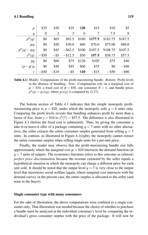
4.1 Bundling 119
p $35 $30 $25 $20 $15 $10 $5
q 0 2 3 6 7 7.5 8
pb(q) $0 $65 $92.5 $160 $177.5 $183.75 $187.5
μq $0 $20 $30.0 $60 $70.0 $75.00 $80.0
pb(q)−μq $0 $45 −$62.5 $100 $107.5 $108.75 $107.5
yb(q) −$50 −$5 −$12.5 $50 $57.5 $58.75 $57.5
pq $0 $60 $75 $120 $105 $75 $40
(p−μ)q $0 $40 $45 $60 $35 $0 −$40
y −$50 −$10 −$5 $10 −$15 −$50 −$90
Table 4.1: Middle: Computations of the profit-maximizing bundle. Bottom: Profit levels
in the absence of bundling. Note: Computations rely on a marginal cost of
μ = $10, a fixed cost of φ = $50, one consumer N = 1, and bundle prices
pb(q) = gcs(q), where gcs(q) is computed by (2.37).
The bottom section of Table 4.1 indicates that the simple monopoly profit-
maximizing price is p = $20, under which the monopoly sells q = 6 units only.
Comparing the profit levels reveals that bundling enhances profit by more than a
factor of five, from y = $10 to yb(7) = $57.5. The difference is also illustrated in
Figure 4.1 (before the fixed cost is subtracted). Thus, by giving the consumer a
take-it-or-leave-it offer of a package containing q = 7 units with no other alterna-
tives, the seller extracts the entire consumer surplus generated from selling q = 7
units. In contrast, as illustrated in Figure 4.1(right), the monopoly cannot extract
the entire consumer surplus when selling single units for a per-unit price.
Finally, the reader may observe that the profit-maximizing bundle size falls
approximately where the marginal cost μ = $10 intersects the demand function (at
q = 7 units of output). The economics literature refers to this outcome as (almost)
perfect price discrimination because the revenue extracted by the seller equals a
hypothetical situation in which the monopoly can charge a different price for each
unit sold. It should be noted that the output level q = 7 is very close to the output
level that maximizes social welfare (again, where marginal cost intersects with the
demand curve); in the present case, the entire surplus is allocated to the seller (and
none to the buyer).
Single consumer type with many consumers
For the sake of illustration, the above computations were confined to a single con-
sumer only. That illustration was needed because the choice of whether to purchase
a bundle must be analyzed at the individual consumer’s level by comparing the in-
dividual’s gross consumer surplus with the price of the package. It will now be

120 Bundling and Tying
shown that the extension from one consumer to many consumers is rather trivial
after the profit-maximizing bundle is selected for a single consumer.
To see this, suppose that there are N = 150 consumers of the same type, each
represented by the demand function illustrated by Figure 4.1 and also on the top
section of Table 4.1. Table 4.1 shows that the profit-maximizing bundle contains
q = 7 units and is sold for a package price of pb(7) = $177.5. With N = 150
consumers, we can write the total profit directly as
yb = N[pb(q)−μq]−φ = 150[177.5−10 ·7]−50 = $16,075. (4.2)
In contrast, the profit when each unit is sold separately is y = N(p− μ)− φ =150(20− 10)− 50 = $1450, which shows again that bundling can be much more
profitable than selling each unit separately.
Algorithm 4.1 suggests a short computer program for selecting the most prof-
itable bundle. This program should input (say, using the Read() command), and
store the discrete demand function based on M ≥ 2 price-quantity observations.
More precisely, the program must input the price p[�] and the quantity demanded
q[�] for each demand observation � = 1, . . . ,M, where p[�] and q[�] are arrays of
dimension M of real-valued demand observations. The program must also input
the seller’s cost parameters μ (marginal cost), φ (fixed cost), and N, which is the
number of consumers with the above demand function.
maxyb← 0; /* Initializing output variable */for � = 1 to M do
/* Main loop over demand observations */if N(gcs[�]−μq[�])−φ ≥maxyb then
/* If higher profit found, store new values */maxyb← N(gcs[�]−μq[�])−φ ; maxqyb← q[�]; maxpyb← gcs[�];
if maxyb ≥ 0 thenwriteln (“The profit-maximizing bundle contains q =”, maxqyb, “units,
and priced at pb =”, maxpyb, “The resulting total profit is yb = ”,
maxyb);
/* Optional: Run Algorithm 3.1 and compare profits */write (“The profit gain from selling a bundle instead of individual units
only is:”, maxyb−maxy)
else write (“Negative profit. Do NOT operate in this market!”)
Algorithm 4.1: Computing the profit-maximizing bundle for a single con-
sumer type with discrete demand.
After inputting the above data, the user must run Algorithm 2.3 to compute
the gross consumer surplus for the inputted discrete demand function, and write
4.1 Bundling 121
the results onto the real-valued M-dimensional array gcs[�], � = 1, . . . ,M, which
should also be stored on the system.
Algorithm 4.1 is rather straightforward. It runs a loop over all observations
� = 1,2, · · · ,M, and computes the profit level, which is the difference between the
bundle’s price (equal to the gross consumer surplus, gcs[�]) and the variable cost,
μq[�]. Each loop also checks whether the computed profit level exceeds the already-
stored value of the maximized profit, maxyb. If the computed level exceeds maxyb,
the newly computed level replaces the previously stored value of maxyb.
Using the same data, Algorithm 4.1 can also be used simultaneously with Algo-
rithm 3.1, which computes the simple monopoly profit-maximizing price per unit.
Therefore, the two algorithms can be easily integrated to perform a comparison be-
tween the profit when the firm bundles, maxyb, and the profit when the firm does
not bundle, maxy.
Single consumer type: Continuous demand approximation
The computation of gross consumer surplus is greatly simplified if a continuous
linear demand function is used instead of the discrete demand function illustrated
in Figure 4.1. In fact, equation (2.39) derives the gross consumer surplus for the
general linear demand function p = α−βq to be
gcs(q) =(α + p)(q−0)
2=
(α +α−βq)(q−0)2
=(2α−βq)q
2. (4.3)
Therefore, for a quick (but less accurate) selection of the profit-maximizing bundle,
the seller can fit a linear curve to the discrete demand function, and then compute
the price by using (4.3) and the known cost parameters.
Using the regression technique described in Section 2.3.2, a linear fitting of
the demand function illustrated by Figure 4.1 and on the top section of Table 4.1
yields p = 36.93− 3.66q. Thus, the estimated coefficients of this linear demand
approximation are α = 36.93 and β = 3.66. The fitted demand curve is illustrated
in Figure 4.2. This demand intersects marginal cost at p = 36.93−3.66q = μ = 10,
hence at q = 7.36 units.
Figure 4.2 shows that profit, defined as y = pb(q)−μq−φ , is maximized when
the firm sells a bundle with q units, where q solves μ = α −βq, hence q = 7.36
for the present example. Clearly, this is only an approximation because if this good
is indivisible, this result hints that the profit-maximizing bundle should consist of
either q = 7 or q = 8 units. Finally, the price of this bundle can be easily found by
computing the gross consumer surplus (4.3). Hence,
pb(7.36) = gcs(7.36) =(2 ·36.93−3.66 ·7.36)7.36
2= $172.67. (4.4)
The resulting profit is then
yb(7.36) = pb(7.36)−7.36μ−φ = 172.67−7.36 ·10−50 = $49.07. (4.5)

122 Bundling and Tying
�
p
•$30
$25
••
$20
$15
$10
2 6 93 4 51
••
•
$35•
Variable cost = 7μ
10.09
� q
p = 36.93−3.66q
pb(7)−7μ
μ
7.36
Figure 4.2: Profit-maximizing single-package bundling using a linear demand approxima-
tion for single consumer type.
Comparing the bundle’s price and profit from the linear demand approximation
(4.4) and (4.5) with the profit computed directly from the discrete data given in
Table 4.1 yields the magnitude of the error generated by the linear approximation.
That is, Table 4.1 indicates that the profit-maximizing bundle has q = 7 units, priced
at pb = $177.5, and earns a profit level yb = $57.5. The analysis under the linear
demand approximation suggests a profit-maximizing bundle of q = 7.36 units, a
price of pb = $172.67, and a resulting profit of yb = $49.07 < $57.5.
Finally, as with the discrete demand case, the linear demand approximation
can be extended to N ≥ 2 consumers of the same type by multiplying revenue and
variable cost by N. For the present example, with N consumers, the profit becomes
yb = N(pb−μq)−φ = N(172.67−7.36 ·10)−50 = 99.07N−50.
The example provided by Figure 4.2 is now generalized to any linear demand
function given by p = α −βq, where α > μ and β > 0. This generalization also
proves our assertion above that with a single consumer type, the profit-maximizing
bundle is determined at the point where the inverse demand function intersects with
the marginal cost. Formally, the seller chooses a bundle with q units to solve
maxq
yb = N [gcs(q)−μq]−φ = N[(2α−βq)q
2−μq
]−φ , (4.6)
where gcs(q) was substituted from (4.3). The first-order condition for selecting the
profit-maximizing bundle implies that
dgcs(q)dq
= α−βq = μ , hence qb =α−μ
β. (4.7)
This condition proves that the profit-maximizing bundle size is determined by in-
tersection of the demand with the marginal cost. Moreover, recall from equation
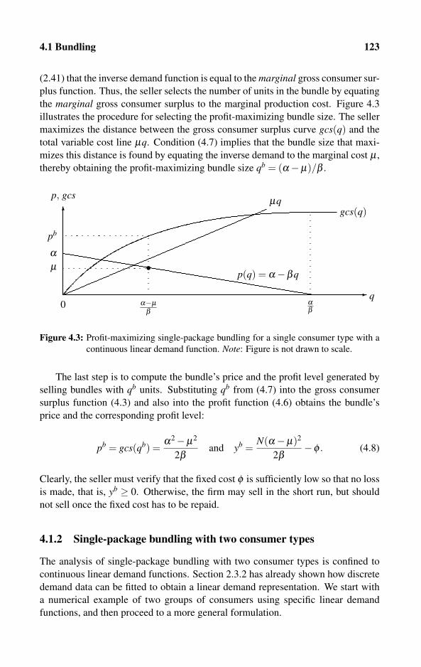
4.1 Bundling 123
(2.41) that the inverse demand function is equal to the marginal gross consumer sur-
plus function. Thus, the seller selects the number of units in the bundle by equating
the marginal gross consumer surplus to the marginal production cost. Figure 4.3
illustrates the procedure for selecting the profit-maximizing bundle size. The seller
maximizes the distance between the gross consumer surplus curve gcs(q) and the
total variable cost line μq. Condition (4.7) implies that the bundle size that maxi-
mizes this distance is found by equating the inverse demand to the marginal cost μ ,
thereby obtaining the profit-maximizing bundle size qb = (α−μ)/β .
�
αβ
α
p, gcs
� q
μ
μq
p(q) = α−βq
gcs(q)
α−μβ
pb
•
0
Figure 4.3: Profit-maximizing single-package bundling for a single consumer type with a
continuous linear demand function. Note: Figure is not drawn to scale.
The last step is to compute the bundle’s price and the profit level generated by
selling bundles with qb units. Substituting qb from (4.7) into the gross consumer
surplus function (4.3) and also into the profit function (4.6) obtains the bundle’s
price and the corresponding profit level:
pb = gcs(qb) =α2−μ2
2βand yb =
N(α−μ)2
2β−φ . (4.8)
Clearly, the seller must verify that the fixed cost φ is sufficiently low so that no loss
is made, that is, yb ≥ 0. Otherwise, the firm may sell in the short run, but should
not sell once the fixed cost has to be repaid.
4.1.2 Single-package bundling with two consumer types
The analysis of single-package bundling with two consumer types is confined to
continuous linear demand functions. Section 2.3.2 has already shown how discrete
demand data can be fitted to obtain a linear demand representation. We start with
a numerical example of two groups of consumers using specific linear demand
functions, and then proceed to a more general formulation.
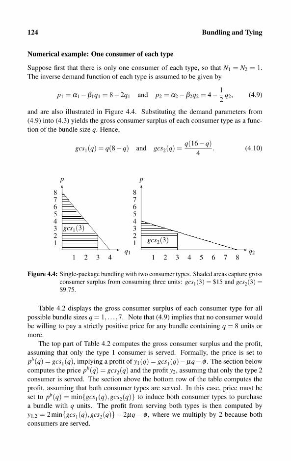
124 Bundling and Tying
Numerical example: One consumer of each type
Suppose first that there is only one consumer of each type, so that N1 = N2 = 1.
The inverse demand function of each type is assumed to be given by
p1 = α1−β1q1 = 8−2q1 and p2 = α2−β2q2 = 4− 1
2q2, (4.9)
and are also illustrated in Figure 4.4. Substituting the demand parameters from
(4.9) into (4.3) yields the gross consumer surplus of each consumer type as a func-
tion of the bundle size q. Hence,
gcs1(q) = q(8−q) and gcs2(q) =q(16−q)
4. (4.10)
2
12345678
1 3 4
� q12
12345678
1 3 4 5 6 7 8
� q2
� ����������
p p
gcs1(3)
gcs2(3)
Figure 4.4: Single-package bundling with two consumer types. Shaded areas capture gross
consumer surplus from consuming three units: gcs1(3) = $15 and gcs2(3) =$9.75.
Table 4.2 displays the gross consumer surplus of each consumer type for all
possible bundle sizes q = 1, . . . ,7. Note that (4.9) implies that no consumer would
be willing to pay a strictly positive price for any bundle containing q = 8 units or
more.
The top part of Table 4.2 computes the gross consumer surplus and the profit,
assuming that only the type 1 consumer is served. Formally, the price is set to
pb(q) = gcs1(q), implying a profit of y1(q) = gcs1(q)−μq−φ . The section below
computes the price pb(q) = gcs2(q) and the profit y2, assuming that only the type 2
consumer is served. The section above the bottom row of the table computes the
profit, assuming that both consumer types are served. In this case, price must be
set to pb(q) = min{gcs1(q),gcs2(q)} to induce both consumer types to purchase
a bundle with q units. The profit from serving both types is then computed by
y1,2 = 2min{gcs1(q),gcs2(q)}− 2μq− φ , where we multiply by 2 because both
consumers are served.

4.1 Bundling 125
q (bundle size) 1 2 3 4 5 6 7
gcs1(q) $7.00 $12 $15.00 $16 $0.00 $0 $0.00
y1(q) $5.00 $8 $9.00 $8 $0.00 $0 $0.00
gcs2(q) $3.75 $7 $9.75 $12 $13.75 $15 $15.75
y2(q) $1.75 $3 $3.75 $4 $3.75 $3 $1.75
min{gcs1,gcs2} $3.75 $7 $9.75 $12 $0.00 $0 $0.00
y1,2(q) $3.50 $6 $7.50 $8 < 0 < 0 < 0
max{y1,y2,y1,2} $5.00 $8 $9.00 $8 $3.75 $3 $1.75
Table 4.2: Computations of the profit-maximizing bundle with two consumer types. Note:
Computations rely on a marginal cost of μ = $2, a fixed cost of φ = $0 (zero),
and one consumer of each type, N1 = N2 = 1.
The last row in Table 4.2 determines the maximum profit associated with each
bundle size q. For example, if the firm sells a bundle with q = 2 units, profit is
maximized at y1 = $8, where the price is set to pb(2) = gcs1(2) = $12 > $7 =gcs2(2). Hence, the type 2 consumer does not buy at this price. Comparing all
the profit levels on the bottom row of Table 4.2 reveals that the profit-maximizing
bundle size has q = 3 units. This bundle is priced at pb(3) = gcs1(3) = $15 >$9.75 = gcs2(3) (see also Figure 4.4), hence only the type 1 consumer buys it, and
the firm earns a profit of y(3) = $9.
To conclude this example, observe from Table 4.2 that for small bundles, where
q = 1,2,3, the firm maximizes profit by selecting a price that excludes the type 2
consumer. If the firm sells q = 4 units in a bundle, it is indifferent as to whether
to price high at pb(4) = gcs1(4) = $16 so only type 1 buys or to price sufficiently
low at pb(4) = gcs2(4) = $12 so both consumer types buy. In either case, the seller
earns y1(4) = y1,2(4) = $8. Bundles of sizes larger than q ≥ 5 units are priced at
pb(q) = gcs2(q) (so the type 1 consumer is excluded) because the willingness to
pay by the type 1 consumer falls below marginal cost at these quantity levels.
Numerical example: Multiple consumers of each type
The calculation results exhibited in Table 4.2 are based on two consumer types,
defined by the demand functions (4.9), and N1 = N2 = 1 (one consumer per type).
We now extend this example to multiple consumers of each type. Formally, sup-
pose that there are N1 = 2 type 1 consumers and N2 = 5 type 2 consumers. Ta-
ble 4.3 modifies Table 4.2 by recalculating the profit levels for each size q bun-
dle for multiple consumers of each type. The recalculated profit levels in Ta-
ble 4.3 are based on y1(q) = 2[gcs1(q)− μq]− φ , y2(q) = 5[gcs2(q)− μq)]− φ ,
and y1,2(q) = (2+5)[p(q)−μq]−φ , where p(q) = min{gcs1(q),gcs2(q)}.
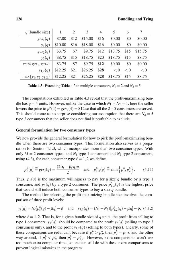
126 Bundling and Tying
q (bundle size) 1 2 3 4 5 6 7
gcs1(q) $7.00 $12 $15.00 $16 $0.00 $0 $0.00
y1(q) $10.00 $16 $18.00 $16 $0.00 $0 $0.00
gcs2(q) $3.75 $7 $9.75 $12 $13.75 $15 $15.75
y2(q) $8.75 $15 $18.75 $20 $18.75 $15 $8.75
min{gcs1,gcs2} $3.75 $7 $9.75 $12 $0.00 $0 $0.00
y1,2(q) $12.25 $21 $26.25 $28 < 0 < 0 < 0
max{y1,y2,y1,2} $12.25 $21 $26.25 $28 $18.75 $15 $8.75
Table 4.3: Extending Table 4.2 to multiple consumers, N1 = 2 and N2 = 5.
The computations exhibited in Table 4.3 reveal that the profit-maximizing bun-
dle has q = 4 units. However, unlike the case in which N1 = N2 = 1, here the seller
lowers the price to pb(4) = gcs2(4) = $12 so that all the 2+5 consumers are served.
This should come as no surprise considering our assumption that there are N2 = 5
type 2 consumers that the seller does not find it profitable to exclude.
General formulation for two consumer types
We now provide the general formulation for how to pick the profit-maximizing bun-
dle when there are two consumer types. This formulation also serves as a prepa-
ration for Section 4.1.3, which incorporates more than two consumer types. With
only M = 2 consumer types, and N1 type 1 consumers and N2 type 2 consumers,
using (4.3), for each consumer type � = 1,2 we define
pb�(q) def= gcs�(q) =
(2α�−β� q)q2
and pb1,2(q) def= min
{pb
1, pb2
}. (4.11)
Thus, p1(q) is the maximum willingness to pay for a size q bundle by a type 1
consumer, and p2(q) by a type 2 consumer. The price pb1,2(q) is the highest price
that would still induce both consumer types to buy a size q bundle.
The method for selecting the profit-maximizing bundle size involves the com-
parison of three profit levels:
y�(q) = N�[pb�(q)−μq]−φ and y1,2(q) = (N1 +N2)[pb
1,2(q)−μq]−φ , (4.12)
where � = 1,2. That is, for a given bundle size of q units, the profit from selling to
type 1 consumers, y1(q), should be compared to the profit y2(q) (selling to type 2
consumers only), and to the profit y1,2(q) (selling to both types). Clearly, some of
these comparisons are redundant because if pb1 > pb
2, then pb2 = p1,2, and the other
way around, if pb1 < pb
2, then pb1 = pb
1,2. However, extra comparisons won’t use
too much extra computer time, so one can still do with these extra comparisons to
prevent logical mistakes in the program.
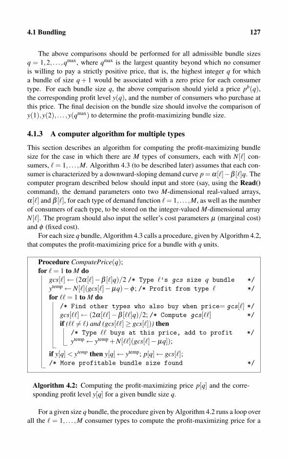
4.1 Bundling 127
The above comparisons should be performed for all admissible bundle sizes
q = 1,2, . . . ,qmax, where qmax is the largest quantity beyond which no consumer
is willing to pay a strictly positive price, that is, the highest integer q for which
a bundle of size q + 1 would be associated with a zero price for each consumer
type. For each bundle size q, the above comparison should yield a price pb(q),the corresponding profit level y(q), and the number of consumers who purchase at
this price. The final decision on the bundle size should involve the comparison of
y(1),y(2), . . . ,y(qmax) to determine the profit-maximizing bundle size.
4.1.3 A computer algorithm for multiple types
This section describes an algorithm for computing the profit-maximizing bundle
size for the case in which there are M types of consumers, each with N[�] con-
sumers, � = 1, . . . ,M. Algorithm 4.3 (to be described later) assumes that each con-
sumer is characterized by a downward-sloping demand curve p = α[�]−β [�]q. The
computer program described below should input and store (say, using the Read()command), the demand parameters onto two M-dimensional real-valued arrays,
α[�] and β [�], for each type of demand function � = 1, . . . ,M, as well as the number
of consumers of each type, to be stored on the integer-valued M-dimensional array
N[�]. The program should also input the seller’s cost parameters μ (marginal cost)
and φ (fixed cost).
For each size q bundle, Algorithm 4.3 calls a procedure, given by Algorithm 4.2,
that computes the profit-maximizing price for a bundle with q units.
Procedure ComputePrice(q);for � = 1 to M do
gcs[�]← (2α[�]−β [�]q)/2 /* Type �’s gcs size q bundle */ytemp← N[�](gcs[�]−μq)−φ ; /* Profit from type � */for �� = 1 to M do
/* Find other types who also buy when price= gcs[�] */gcs[��]← (2α[��]−β [��]q)/2; /* Compute gcs[��] */if (�� �= �) and (gcs[��]≥ gcs[�])) then
/* Type �� buys at this price, add to profit */ytemp← ytemp +N[��](gcs[�]−μq]);
if y[q] < ytemp then y[q]← ytemp; p[q]← gcs[�];/* More profitable bundle size found */
Algorithm 4.2: Computing the profit-maximizing price p[q] and the corre-
sponding profit level y[q] for a given bundle size q.
For a given size q bundle, the procedure given by Algorithm 4.2 runs a loop over
all the � = 1, . . . ,M consumer types to compute the profit-maximizing price for a
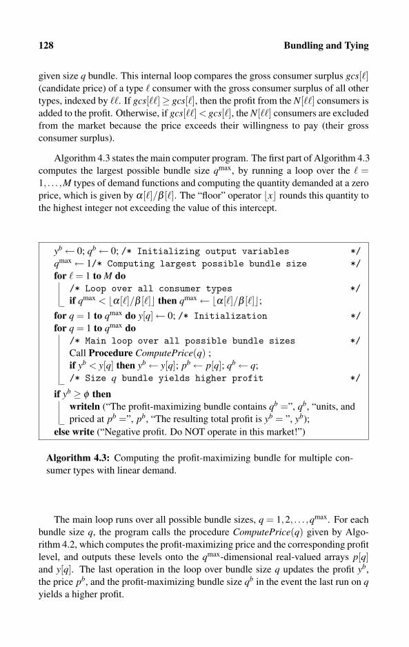
128 Bundling and Tying
given size q bundle. This internal loop compares the gross consumer surplus gcs[�](candidate price) of a type � consumer with the gross consumer surplus of all other
types, indexed by ��. If gcs[��]≥ gcs[�], then the profit from the N[��] consumers is
added to the profit. Otherwise, if gcs[��] < gcs[�], the N[��] consumers are excluded
from the market because the price exceeds their willingness to pay (their gross
consumer surplus).
Algorithm 4.3 states the main computer program. The first part of Algorithm 4.3
computes the largest possible bundle size qmax, by running a loop over the � =1, . . . ,M types of demand functions and computing the quantity demanded at a zero
price, which is given by α[�]/β [�]. The “floor” operator �x� rounds this quantity to
the highest integer not exceeding the value of this intercept.
yb← 0; qb← 0; /* Initializing output variables */qmax← 1/* Computing largest possible bundle size */for � = 1 to M do
/* Loop over all consumer types */if qmax < �α[�]/β [�]� then qmax← �α[�]/β [�]�;
for q = 1 to qmax do y[q]← 0; /* Initialization */for q = 1 to qmax do
/* Main loop over all possible bundle sizes */Call Procedure ComputePrice(q) ;
if yb < y[q] then yb← y[q]; pb← p[q]; qb← q;
/* Size q bundle yields higher profit */
if yb ≥ φ thenwriteln (“The profit-maximizing bundle contains qb =”, qb, “units, and
priced at pb =”, pb, “The resulting total profit is yb = ”, yb);
else write (“Negative profit. Do NOT operate in this market!”)
Algorithm 4.3: Computing the profit-maximizing bundle for multiple con-
sumer types with linear demand.
The main loop runs over all possible bundle sizes, q = 1,2, . . . ,qmax. For each
bundle size q, the program calls the procedure ComputePrice(q) given by Algo-
rithm 4.2, which computes the profit-maximizing price and the corresponding profit
level, and outputs these levels onto the qmax-dimensional real-valued arrays p[q]and y[q]. The last operation in the loop over bundle size q updates the profit yb,
the price pb, and the profit-maximizing bundle size qb in the event the last run on qyields a higher profit.
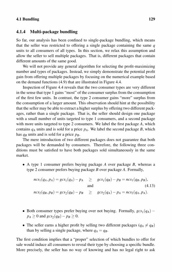
4.1 Bundling 129
4.1.4 Multi-package bundling
So far, our analysis has been confined to single-package bundling, which means
that the seller was restricted to offering a single package containing the same qunits to all consumers of all types. In this section, we relax this assumption and
allow the seller to sell multiple packages. That is, different packages that contain
different amounts of the same good.
We will not provide any general algorithm for selecting the profit-maximizing
number and types of packages. Instead, we simply demonstrate the potential profit
gain from offering multiple packages by focusing on the numerical example based
on the demand functions (4.9) that are illustrated in Figure 4.4.
Inspection of Figure 4.4 reveals that the two consumer types are very different
in the sense that type 1 gains “most” of the consumer surplus from the consumption
of the first few units. In contrast, the type 2 consumer gains “more” surplus from
the consumption of a larger amount. This observation should hint at the possibility
that the seller may be able to extract a higher surplus by offering two different pack-
ages, rather than a single package. That is, the seller should design one package
with a small number of units targeted to type 1 consumers, and a second package
with more units targeted to type 2 consumers. We label the first package A, which
contains qA units and is sold for a price pA. We label the second package B, which
has qB units and is sold for a price pB.
The mere introduction of two different packages does not guarantee that both
packages will be demanded by consumers. Therefore, the following three con-
ditions must be satisfied to have both packages sold simultaneously in the same
market.
• A type 1 consumer prefers buying package A over package B, whereas a
type 2 consumer prefers buying package B over package A. Formally,
ncs1(qA, pA) = gcs1(qA)− pA ≥ gcs1(qB)− pB = ncs1(qB, pB),and (4.13)
ncs2(qB, pB) = gcs2(qB)− pB ≥ gcs2(qA)− pA = ncs2(qA, pA).
• Both consumer types prefer buying over not buying. Formally, gcs1(qA)−pA ≥ 0 and gcs2(qB)− pB ≥ 0.
• The seller earns a higher profit by selling two different packages (qA �= qB)than by selling a single package, where qA = qB.
The first condition implies that a “proper” selection of which bundles to offer for
sale would induce all consumers to reveal their type by choosing a specific bundle.
More precisely, the seller has no way of knowing and has no legal right to ask
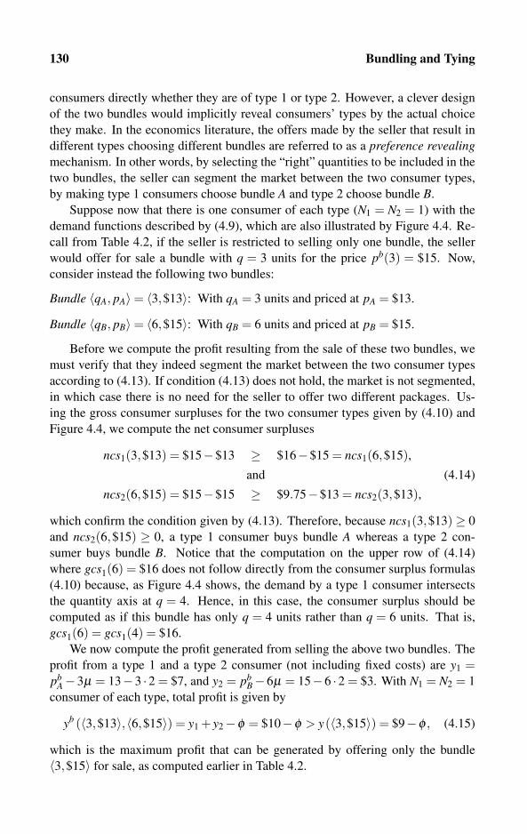
130 Bundling and Tying
consumers directly whether they are of type 1 or type 2. However, a clever design
of the two bundles would implicitly reveal consumers’ types by the actual choice
they make. In the economics literature, the offers made by the seller that result in
different types choosing different bundles are referred to as a preference revealingmechanism. In other words, by selecting the “right” quantities to be included in the
two bundles, the seller can segment the market between the two consumer types,
by making type 1 consumers choose bundle A and type 2 choose bundle B.
Suppose now that there is one consumer of each type (N1 = N2 = 1) with the
demand functions described by (4.9), which are also illustrated by Figure 4.4. Re-
call from Table 4.2, if the seller is restricted to selling only one bundle, the seller
would offer for sale a bundle with q = 3 units for the price pb(3) = $15. Now,
consider instead the following two bundles:
Bundle 〈qA, pA〉= 〈3,$13〉: With qA = 3 units and priced at pA = $13.
Bundle 〈qB, pB〉= 〈6,$15〉: With qB = 6 units and priced at pB = $15.
Before we compute the profit resulting from the sale of these two bundles, we
must verify that they indeed segment the market between the two consumer types
according to (4.13). If condition (4.13) does not hold, the market is not segmented,
in which case there is no need for the seller to offer two different packages. Us-
ing the gross consumer surpluses for the two consumer types given by (4.10) and
Figure 4.4, we compute the net consumer surpluses
ncs1(3,$13) = $15−$13 ≥ $16−$15 = ncs1(6,$15),and (4.14)
ncs2(6,$15) = $15−$15 ≥ $9.75−$13 = ncs2(3,$13),
which confirm the condition given by (4.13). Therefore, because ncs1(3,$13) ≥ 0
and ncs2(6,$15) ≥ 0, a type 1 consumer buys bundle A whereas a type 2 con-
sumer buys bundle B. Notice that the computation on the upper row of (4.14)
where gcs1(6) = $16 does not follow directly from the consumer surplus formulas
(4.10) because, as Figure 4.4 shows, the demand by a type 1 consumer intersects
the quantity axis at q = 4. Hence, in this case, the consumer surplus should be
computed as if this bundle has only q = 4 units rather than q = 6 units. That is,
gcs1(6) = gcs1(4) = $16.
We now compute the profit generated from selling the above two bundles. The
profit from a type 1 and a type 2 consumer (not including fixed costs) are y1 =pb
A−3μ = 13−3 ·2 = $7, and y2 = pbB−6μ = 15−6 ·2 = $3. With N1 = N2 = 1
consumer of each type, total profit is given by
yb (〈3,$13〉,〈6,$15〉) = y1 + y2−φ = $10−φ > y(〈3,$15〉) = $9−φ , (4.15)
which is the maximum profit that can be generated by offering only the bundle
〈3,$15〉 for sale, as computed earlier in Table 4.2.

4.2 Tying 131
Finally, note that despite the fact that bundles 〈qA, pbA〉= 〈3,$13〉 and 〈qB, pb
B〉=〈6,$15〉 indeed generate a higher profit than that obtained from selling only the
single bundle 〈q, pb〉 = 〈3,$15〉 computed on Table 4.2, these bundles still do not
maximize profit in the sense that one can still find different bundles that generate
an even higher profit. The reader is referred to Exercise 4 at the end of this chapter
for the computation of such a profit-enhancing bundle.
4.2 Tying
Tying refers to the sale of packages containing different products and/or services
(see Definition 4.1). This is in contrast to bundling, in which packages contain
several units of the same product or service. Tying is practiced in a wide variety
of industries. For example, most cable TV operators offer packages containing a
variety of channels without giving subscribers the option of buying each channel
separately. This practice hints that tying enhances sellers’ profit compared with
selling each good separately.
Another example of tying are travel agencies that provide organized tours con-
taining accommodations, transportation, and sightseeing in a single package. The
last example refers to the practice of tying of related services. However, tying is
also observed for unrelated goods – for example, a bookstore tying a T-shirt (or a
cup of coffee) with a purchase of a certain book.
For the purpose of this book, the following definition classifies different meth-
ods of tying:
DEFINITION 4.3
The seller is said to be practicing
(a) No tying (NT) if each good is sold separately from all other goods.
(b) Pure tying (PT) (or, more simply, tying) if only one package containing all
goods is offered for sale. Goods cannot be purchased separately.
(c) Mixed tying (MT) if all goods are offered for sale in a single package, and in
addition, each good can be purchased separately.
(d) Multi-package tying (MPT) if more than one package is offered for sale and
at least two packages contain two or more different goods.
Figure 4.5 illustrates how different types of consumers choose what to buy under no
tying, pure tying and mixed tying, when there are only two goods, labeled A and B.
Good A could, for example, denote a music CD played by the Austrian Symphony
Orchestra, whereas good B could be a CD by the Beatles. We assume that each
consumer demands at most one CD of each group.
Under no tying, consumers, who buy at most one unit of each good, are offered
good A for a price pA and good B for a price pB. A type � consumer, � = 1, . . . ,M,
will buy a unit of A if the price does not exceed the consumer’s valuation for good A,
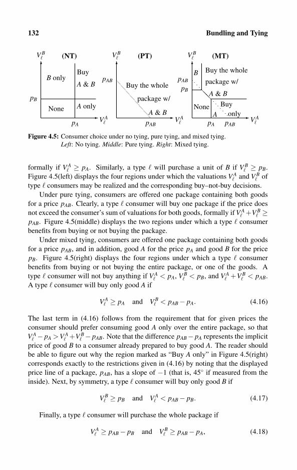
132 Bundling and Tying
�
�
V A�
V B� (NT)
�
�
V A�
V B� (PT)
�
�
V A�
V B� (MT)
pB
pA
None
B onlyBuy
A & B
A only
pAB
pABBuy the whole
A & B
package w/��
B
pA
pB
pAB
pAB
Buy
A onlyNone
Buy the whole
package w/
A & B
Figure 4.5: Consumer choice under no tying, pure tying, and mixed tying.
Left: No tying. Middle: Pure tying. Right: Mixed tying.
formally if V A� ≥ pA. Similarly, a type � will purchase a unit of B if V B
� ≥ pB.
Figure 4.5(left) displays the four regions under which the valuations V A� and V B
� of
type � consumers may be realized and the corresponding buy–not-buy decisions.
Under pure tying, consumers are offered one package containing both goods
for a price pAB. Clearly, a type � consumer will buy one package if the price does
not exceed the consumer’s sum of valuations for both goods, formally if V A� +V B
� ≥pAB. Figure 4.5(middle) displays the two regions under which a type � consumer
benefits from buying or not buying the package.
Under mixed tying, consumers are offered one package containing both goods
for a price pAB, and in addition, good A for the price pA and good B for the price
pB. Figure 4.5(right) displays the four regions under which a type � consumer
benefits from buying or not buying the entire package, or one of the goods. A
type � consumer will not buy anything if V A� < pA, V B
� < pB, and V A� +V B
� < pAB.
A type � consumer will buy only good A if
V A� ≥ pA and V B
� < pAB− pA. (4.16)
The last term in (4.16) follows from the requirement that for given prices the
consumer should prefer consuming good A only over the entire package, so that
V A� − pA >V A
� +V B� − pAB. Note that the difference pAB− pA represents the implicit
price of good B to a consumer already prepared to buy good A. The reader should
be able to figure out why the region marked as “Buy A only” in Figure 4.5(right)
corresponds exactly to the restrictions given in (4.16) by noting that the displayed
price line of a package, pAB, has a slope of −1 (that is, 45◦ if measured from the
inside). Next, by symmetry, a type � consumer will buy only good B if
V B� ≥ pB and V A
� < pAB− pB. (4.17)
Finally, a type � consumer will purchase the whole package if
V A� ≥ pAB− pB and V B
� ≥ pAB− pA, (4.18)

4.2 Tying 133
which follows directly from the requirement that
V A� +V A
� − pAB ≥max{
V A� − pA,V B
� − pB}
.
The classifications made by Definition 4.3 imply that the difference between
mixed tying and multi-package tying is that mixed tying offers consumers a choice
between two extreme types of packages: They can either buy one package contain-
ing all goods tied in a single basket or can purchase each good separately. In con-
trast, multi-package tying offers consumers a wider variety of packages, in which
packages may contain only a subset of all the goods offered by the seller (in contrast
to packages offered under pure and mixed tying, which contain all goods).
Definition 4.3 implicitly assumes that packages contain at most one unit of each
good. That is, no package contains two or more units of the same good. However, in
principle, sellers should experiment with combining tying with bundling, whereby
some goods may be offered in large quantities in addition to being tied to different
products and services. We rule out this possibility by assuming that consumers have
a single-unit demand for each good, as illustrated in Figure 4.6. Thus, the consumer
buys at most one unit as long as the price does not exceed a certain valuation level,
denoted by V , which reflects the consumer’s maximum willingness to pay.
�
�
qA1
pA
V A1
1
�
�
qB1
pB
1
�
�
qA2
pA
1
�
�
pB
V B2
10 0 0 0
V B1 V A
2
qB2
•
• •
•
Figure 4.6: Pure tying: Negatively correlated unit demand functions.
4.2.1 Pure tying: Theory and examples
Consider a seller who offers for sale more than one good. By goods, we refer to
products or services, or both. The seller has only two options: (a) Offer all the
goods in a single package, for a package price, or (b) Sell each good separately at
a per-unit price. We now demonstrate the potential gain from tying in a series of
examples by varying the number of consumer types and the number of goods that
the seller can combine into a single package.
Two consumers and two goods
Consider two goods indexed by i = A,B and two consumers indexed by � = 1,2.
Each consumer buys at most one unit of good A, good B, or both. Figure 4.6
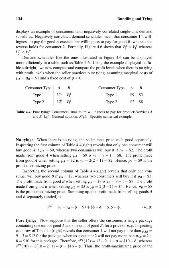
134 Bundling and Tying
displays an example of consumers with negatively correlated single-unit demand
schedules. Negatively correlated demand schedules mean that consumer 1’s will-
ingness to pay for good A exceeds her willingness to pay for good B, whereas the
reverse holds for consumer 2. Formally, Figure 4.6 shows that V A1 > V B
1 whereas
V A2 < V B
2 .
Demand schedules like the ones illustrated in Figure 4.6 can be displayed
more efficiently in a table such as Table 4.6. Using the example displayed in Ta-
ble 4.4(right), we now compute and compare the profit levels when there is no tying
with profit levels when the seller practices pure tying, assuming marginal costs of
μA = μB = $1 and a fixed cost of φ ≥ 0.
Consumer Type A B
Type 1 V A1 V B
1
Type 2 V B2 V B
2
Consumer Type A B
Type 1 $9 $3
Type 2 $2 $8
Table 4.4: Pure tying: Consumers’ maximum willingness to pay for products/services Aand B. Left: General notation. Right: Specific numerical example.
No tying: When there is no tying, the seller must price each good separately.
Inspecting the first column of Table 4.4(right) reveals that only one consumer will
buy good A if pA = $9, whereas two consumers will buy it if pA = $2. The profit
made from good A when setting pA = $9 is yA = 9− 1 = $8. The profit made
from good A when setting pA = $2 is yA = 2(2− 1) = $2. Hence, pA = $9 is the
profit-maximizing price.
Inspecting the second column of Table 4.4(right) reveals that only one con-
sumer will buy good B if pB = $8, whereas two consumers will buy it if pB = $3.
The profit made from good B when setting pB = $8 is yB = 8−1 = $7. The profit
made from good B when setting pB = $3 is yB = 2(3− 1) = $4. Hence, pB = $8
is the profit-maximizing price. Summing up, the profit made from selling goods Aand B separately (untied) is
yNT = yA + yB−φ = $7+$8−φ = $15−φ . (4.19)
Pure tying: Now suppose that the seller offers the customers a single package
containing one unit of good A and one unit of good B, for a price of pAB. Inspecting
each row of Table 4.4(right) reveals that consumer 1 will not pay more than pAB =9+3 = $12 for the package, whereas consumer 2 will not pay more than pAB = 2+8 = $10 for this package. Therefore, yPT(12) = 12−2 ·1−φ = $10−φ , whereas
yPT(10) = 2(10− 2 · 1)− φ = $16− φ . Thus, the profit-maximizing price of the
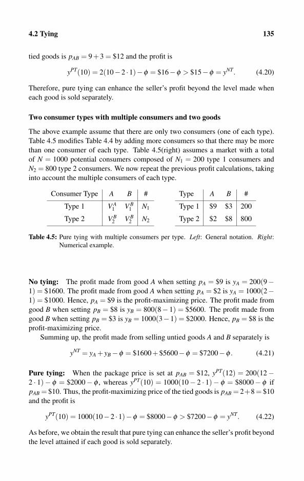
4.2 Tying 135
tied goods is pAB = 9+3 = $12 and the profit is
yPT(10) = 2(10−2 ·1)−φ = $16−φ > $15−φ = yNT. (4.20)
Therefore, pure tying can enhance the seller’s profit beyond the level made when
each good is sold separately.
Two consumer types with multiple consumers and two goods
The above example assume that there are only two consumers (one of each type).
Table 4.5 modifies Table 4.4 by adding more consumers so that there may be more
than one consumer of each type. Table 4.5(right) assumes a market with a total
of N = 1000 potential consumers composed of N1 = 200 type 1 consumers and
N2 = 800 type 2 consumers. We now repeat the previous profit calculations, taking
into account the multiple consumers of each type.
Consumer Type A B #
Type 1 V A1 V B
1 N1
Type 2 V B2 V B
2 N2
Type A B #
Type 1 $9 $3 200
Type 2 $2 $8 800
Table 4.5: Pure tying with multiple consumers per type. Left: General notation. Right:Numerical example.
No tying: The profit made from good A when setting pA = $9 is yA = 200(9−1) = $1600. The profit made from good A when setting pA = $2 is yA = 1000(2−1) = $1000. Hence, pA = $9 is the profit-maximizing price. The profit made from
good B when setting pB = $8 is yB = 800(8− 1) = $5600. The profit made from
good B when setting pB = $3 is yB = 1000(3−1) = $2000. Hence, pB = $8 is the
profit-maximizing price.
Summing up, the profit made from selling untied goods A and B separately is
yNT = yA + yB−φ = $1600+$5600−φ = $7200−φ . (4.21)
Pure tying: When the package price is set at pAB = $12, yPT(12) = 200(12−2 · 1)− φ = $2000− φ , whereas yPT(10) = 1000(10− 2 · 1)− φ = $8000− φ if
pAB = $10. Thus, the profit-maximizing price of the tied goods is pAB = 2+8 = $10
and the profit is
yPT(10) = 1000(10−2 ·1)−φ = $8000−φ > $7200−φ = yNT. (4.22)
As before, we obtain the result that pure tying can enhance the seller’s profit beyond
the level attained if each good is sold separately.
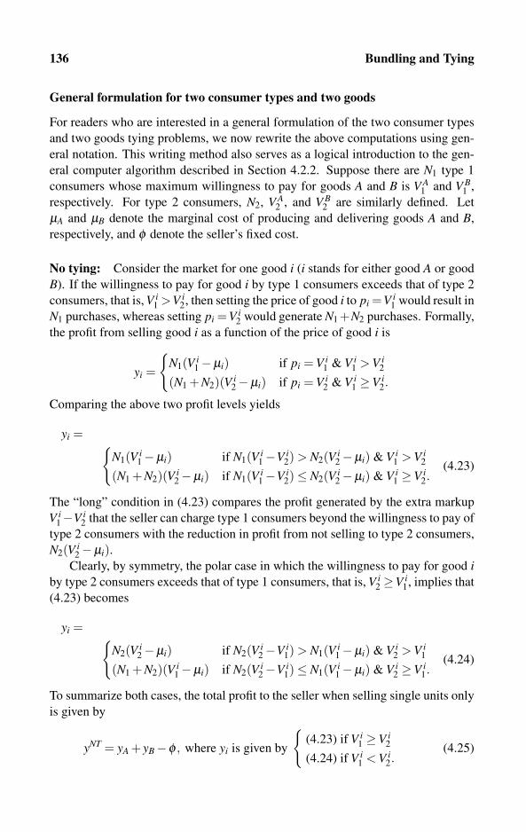
136 Bundling and Tying
General formulation for two consumer types and two goods
For readers who are interested in a general formulation of the two consumer types
and two goods tying problems, we now rewrite the above computations using gen-
eral notation. This writing method also serves as a logical introduction to the gen-
eral computer algorithm described in Section 4.2.2. Suppose there are N1 type 1
consumers whose maximum willingness to pay for goods A and B is V A1 and V B
1 ,
respectively. For type 2 consumers, N2, V A2 , and V B
2 are similarly defined. Let
μA and μB denote the marginal cost of producing and delivering goods A and B,
respectively, and φ denote the seller’s fixed cost.
No tying: Consider the market for one good i (i stands for either good A or good
B). If the willingness to pay for good i by type 1 consumers exceeds that of type 2
consumers, that is, V i1 >V i
2, then setting the price of good i to pi =V i1 would result in
N1 purchases, whereas setting pi =V i2 would generate N1 +N2 purchases. Formally,
the profit from selling good i as a function of the price of good i is
yi =
{N1(V i
1−μi) if pi = V i1 & V i
1 > V i2
(N1 +N2)(V i2−μi) if pi = V i
2 & V i1 ≥V i
2.
Comparing the above two profit levels yields
yi = {N1(V i
1−μi) if N1(V i1−V i
2) > N2(V i2−μi) & V i
1 > V i2
(N1 +N2)(V i2−μi) if N1(V i
1−V i2)≤ N2(V i
2−μi) & V i1 ≥V i
2.(4.23)
The “long” condition in (4.23) compares the profit generated by the extra markup
V i1−V i
2 that the seller can charge type 1 consumers beyond the willingness to pay of
type 2 consumers with the reduction in profit from not selling to type 2 consumers,
N2(V i2−μi).
Clearly, by symmetry, the polar case in which the willingness to pay for good iby type 2 consumers exceeds that of type 1 consumers, that is, V i
2 ≥V i1, implies that
(4.23) becomes
yi = {N2(V i
2−μi) if N2(V i2−V i
1) > N1(V i1−μi) & V i
2 > V i1
(N1 +N2)(V i1−μi) if N2(V i
2−V i1)≤ N1(V i
1−μi) & V i2 ≥V i
1.(4.24)
To summarize both cases, the total profit to the seller when selling single units only
is given by
yNT = yA + yB−φ , where yi is given by
{(4.23) if V i
1 ≥V i2
(4.24) if V i1 < V i
2.(4.25)

4.2 Tying 137
Pure tying: The seller must determine a single price, pAB, for a package contain-
ing one unit of A and one unit of B. A type 1 consumer will buy the package if
pAB ≤ V A1 +V B
1 . Similarly, a type 2 will buy if pAB ≤ V A2 +V B
2 . The method for
selecting the profit-maximizing price for this package is very similar to the method
of selecting the price for a single good. The decision of how to price this package
depends also on the types’ relative willingness to pay for this package, that is, on
whether V A1 +V B
1 > V A2 +V B
2 , or the other way around. This ordering determines
which type of consumer should become a candidate for exclusion. Exclusion is
accomplished by setting a price above a type’s willingness to pay but below that
of the other type, taking into consideration that the marginal cost of the package is
μA + μB.
If the willingness to pay of type 1 consumers exceeds that of type 2 consumers,
that is, V A1 +V B
1 > V A2 +V B
2 , then setting the price pAB = V A1 +V B
1 would result in
N1 purchases, whereas setting pAB = V A2 +V B
2 would generate N1 +N2 purchases.
Formally, if V A1 +V B
1 > V A2 +V B
2 , the profit from selling the tied goods in a
single package as a function of its price is
yPT =
{N1(V A
1 +V B1 −μA−μB) if pAB = V A
1 +V B1
(N1 +N2)(V A2 +V B
2 −μA−μB) if pAB = V A2 +V B
2 .
Similarly, if V A2 +V B
2 > V A1 +V B
1 , the profit from selling the tied goods in a single
package as a function of its price is
yPT =
{N2(V A
2 +V B2 −μA−μB) if pAB = V A
2 +V B2
(N1 +N2)(V A1 +V B
1 −μA−μB) if pAB = V A1 +V B
1 .
Comparing the above two profit levels for the case in which V A1 +V B
1 >V A2 +V B
2
yields
yPT = ⎧⎪⎪⎨⎪⎪⎩
N1(V A1 +V B
1 −μA−μB)−φ ifN1(V A
1 +V B1 −V A
2 −V B2 )
N2(V A2 +V B
2 −μA−μB) > 1
(N1 +N2)(V A2 +V B
2 −μA−μB)−φ ifN1(V A
1 +V B1 −V A
2 −V B2 )
N2(V A2 +V B
2 −μA−μB) ≤ 1.
(4.26)
The condition in (4.26) has the same interpretation as the condition in (4.23). It
compares the profit generated by the extra markup, V A1 +V B
1 −V A2 −V B
2 , the seller
can charge type 1 consumers beyond the willingness to pay of type 2 consumers
with the reduction in profit from not selling to type 2 consumers, N2(V A2 +V B
2 −μA−μB). Next, comparing the above two profit levels for the case in which V A
2 +
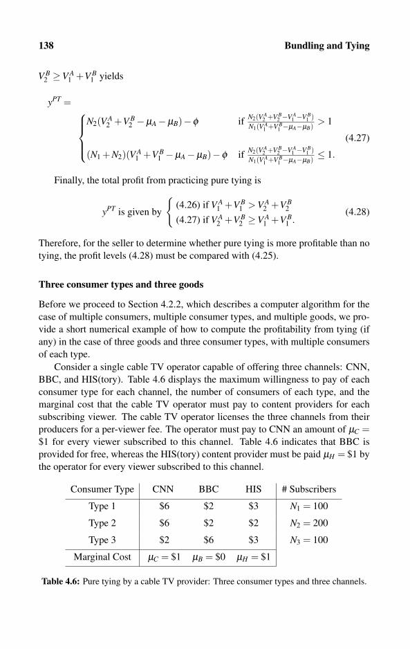
138 Bundling and Tying
V B2 ≥V A
1 +V B1 yields
yPT = ⎧⎪⎪⎨⎪⎪⎩
N2(V A2 +V B
2 −μA−μB)−φ ifN2(V A
2 +V B2 −V A
1 −V B1 )
N1(V A1 +V B
1 −μA−μB) > 1
(N1 +N2)(V A1 +V B
1 −μA−μB)−φ ifN2(V A
2 +V B2 −V A
1 −V B1 )
N1(V A1 +V B
1 −μA−μB) ≤ 1.
(4.27)
Finally, the total profit from practicing pure tying is
yPT is given by
{(4.26) if V A
1 +V B1 > V A
2 +V B2
(4.27) if V A2 +V B
2 ≥V A1 +V B
1 .(4.28)
Therefore, for the seller to determine whether pure tying is more profitable than no
tying, the profit levels (4.28) must be compared with (4.25).
Three consumer types and three goods
Before we proceed to Section 4.2.2, which describes a computer algorithm for the
case of multiple consumers, multiple consumer types, and multiple goods, we pro-
vide a short numerical example of how to compute the profitability from tying (if
any) in the case of three goods and three consumer types, with multiple consumers
of each type.
Consider a single cable TV operator capable of offering three channels: CNN,
BBC, and HIS(tory). Table 4.6 displays the maximum willingness to pay of each
consumer type for each channel, the number of consumers of each type, and the
marginal cost that the cable TV operator must pay to content providers for each
subscribing viewer. The cable TV operator licenses the three channels from their
producers for a per-viewer fee. The operator must pay to CNN an amount of μC =$1 for every viewer subscribed to this channel. Table 4.6 indicates that BBC is
provided for free, whereas the HIS(tory) content provider must be paid μH = $1 by
the operator for every viewer subscribed to this channel.
Consumer Type CNN BBC HIS # Subscribers
Type 1 $6 $2 $3 N1 = 100
Type 2 $6 $2 $2 N2 = 200
Type 3 $2 $6 $3 N3 = 100
Marginal Cost μC = $1 μB = $0 μH = $1
Table 4.6: Pure tying by a cable TV provider: Three consumer types and three channels.

4.2 Tying 139
No tying: Each channel is sold separately to potential viewers. Inspecting Ta-
ble 4.6 reveals that the profit from selling CNN at the price pC = $6 is yC(6) =300(6−1) = $1500. When the price is lowered to pC = $2, yC(2) = 400(2−1) =$400 < $1500.
Table 4.6 also reveals that the profit from selling BBC at the price pB = $6
is yB(6) = 100(6− 0) = $600. When the price is lowered to pB = $2, yB(2) =400(2−0) = $800 > $600.
The profit from selling HIS at the price pH = $3 is yH(3) = 200(3−1) = $400.
When the price is lowered to pH = $2, yH(2) = 400(2−1) = $400.
Summing up, the maximum total profit that can be generated without tying is
yNT = yC + yB + yH −φ = 1500+800+400−φ = $2700−φ . (4.29)
Pure tying: Suppose now that the cable TV operator allows viewers to purchase
one package containing all three channels for a price of pPT and offers no separate
channels. Inspecting Table 4.6 reveals that type 1 and type 3 consumers will not
pay more than $11 for this package, and that type 2 will not pay more than $10.
If the seller sets pCBH = $11, the profit is yPT(11) = (100+100)(11−2)−φ =$1800− φ . If the seller lowers the price to pCBH = $10, the profit is yPT(10) =400(10−2)−φ = $3200−φ . Hence,
yPT = $3200−φ > $2700−φ = yNT, (4.30)
which shows that practicing pure tying is profit enhancing for this cable TV opera-
tor.
4.2.2 Pure tying versus no tying: Computer algorithms
Algorithm 4.4 computes the profit-maximizing prices and the corresponding profit
levels when all goods are sold separately (no tying). Then, Algorithm 4.5 com-
putes the package price and profit for the case in which all goods are sold in
a single package (pure tying). These two programs should input (say, using the
Read() command) the following parameters: M ≥ 2, which is the number of con-
sumer types; N[�], the number of consumers of each type � = 1, . . . ,M; and the set
of goods, B. For example, Table 4.6 displays an example of three goods where
B = {CNN,BBC,HIS}. Then, the program must input consumers’ valuations
(maximum willingness to pay) for each good and store them onto the array V [�, i],where � is the consumer type and i ∈B is the name of a good. The program should
also input the seller’s unit costs of producing each good μ[i], i ∈B, and the fixed
cost φ .
Before running Algorithm 4.4, the program should run Algorithm 3.2, which
generates all the 2M possible selections (subsets) of consumer types. The present
algorithm uses these selections by searching for the highest price under the con-
straint that all the consumers in a particular selection will be willing to pay. Then,

140 Bundling and Tying
yNT←−φ ; /* Subtracting fixed cost from total profit */for i ∈B do
/* Loop over all goods i */pNT[i]← 0; yNT[i]← 0; /* Initial price & profit good i */for j = 1 to 2M−1 do
/* Loop over consumer type selections j */p[ j, i]←V [1, i]; y[ j]← 0; /* Initial price and profit */for � = 2 to M do
/* Finding max possible price under selection j */if p[ j, i] ·Sel[ j, �] > V [�, i] then p[ j, i]←V [�, i]; /* Reduce
price if type � is excluded from selection j */
for � = 1 to M do/* Profits from all types under selection j */y[ j]← y[ j]+{(p[ j, i]−μ[i])N[�]} ·Sel[ j, �];
if yNT[i] < y[ j] then yNT[i]← y[ j]; pNT[i]← p[ j, i]; /* Higherprofit for good i found in selection j */
yNT← yNT + yNT[i]; /* Add profits from all goods i */
writeln (“Total profit made under no tying yNT =”, yNT);
for i ∈B dowrite (“The price of good”, i, “is pi =”, p[i]);writeln (“The profit from selling good”, i, is yi =”, yNT[i]);
Algorithm 4.4: Computing profits under no tying with multiple consumer
types and multiple goods.
the profits from all selections are compared to find the most profitable selection of
consumer types. Algorithm 3.2 writes these subsets onto an array of arrays that we
call Sel (for selection of consumer types). The selection of the served consumer
types is indexed by j = 0, . . . ,2M − 1 (not i, in contrast to Algorithm 3.2). Thus,
Sel[ j, �] is an array of arrays of binary variables with dimension (2M)×M. For
example, in the case of M = 3 consumer types, Sel[7,2] = 1 implies that type 2
consumers are served under the seventh possible selection. Also, Sel[6,2] = 0 im-
plies that type 2 consumers are not served under the sixth possible selection, and
so on.
As for output variables, pNT[i] and yNT[i], i ∈ B store the profit-maximizing
prices when goods are sold separately (no tying), and the profit made from the sale
of each good i. Algorithm 4.4 can be explained as follows: It runs a loop over
all goods i ∈B to compute the profit-maximizing price pNT[i]. Then, it runs an
inner loop over all possible selections of subsets of consumer types indexed by
j = 1, . . . ,2M−1. For each selection of consumer types j, the program determines

4.2 Tying 141
the maximum price for which all the consumer types in selection j would find
it beneficial to purchase. That is, when this loop ends, the price is set so that
p[ j, i] ≤ V [�, i] for every consumer type � belonging to selection j. The next loop
over consumer types � adds up the profit earned from each type in selection j by
multiplying the marginal profit by the number of consumers N[�], and storing on
y[ j].Finally, before advancing the counter of type selection j, the program checks
whether the profit generated by selling to selection j is higher than yNT[i], which is
the highest profit on good i so far. If it is higher, p[i] and yNT[i] are updated. Before
the outer loop on good i ends, the program adds the profit made from the separate
sale of good i, yNT[i], to the total profit yNT earned from all goods combined.
Algorithm 4.5 computes the profit-maximizing price and the corresponding
profit when the seller offers all goods in a single package (pure tying). Then,
this profit is compared with the profit under no tying already computed by Al-
gorithm 4.4.
pPT← 0; yPT←−φ ; μ ← 0; /* Initialization */for i ∈B do μ ← μ + μ[i]; /* Production cost of a package */for � = 1 to M do
V [�]← 0; /* Computing type �’s willingness to pay */for i ∈B do V [�]←V [�]+V [�, i]; /* for the whole package */
for j = 1 to 2M−1 do/* Loop over subsets of consumer type selections j */p[ j]←V [1]; y[ j]← 0; /* Initial price & profit for j */for � = 1 to M do
/* Finding max possible price for selection j */if p[ j] ·Sel[ j, �] > V [�] then p[ j]←V [�]; /* Reduce price if
type � is excluded from selection j */
for � = 1 to M do/* Add profits from all types under selection j */y[ j]← y[ j]+{(p[ j]−μ)N[�]} ·Sel[ j, �];
if yPT < y[ j] then yPT← y[ j]; pPT← p[ j]; /* Selection j yieldshigher profit. Select package price p[ j] */
writeln (“Total profit made under pure tying is yPT =”, yPT), “The package
price is pPT =”, pPT);
write (“The profit gain (loss if negative) from pure tying over no tying is”,
yPT− yNT); /* Comparing with Algorithm 4.4 */
Algorithm 4.5: Computing profits under pure tying with multiple consumer
types and multiple goods.
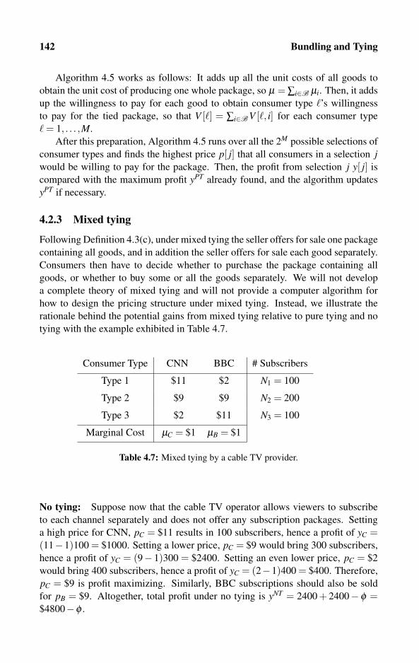
142 Bundling and Tying
Algorithm 4.5 works as follows: It adds up all the unit costs of all goods to
obtain the unit cost of producing one whole package, so μ = ∑i∈B μi. Then, it adds
up the willingness to pay for each good to obtain consumer type �’s willingness
to pay for the tied package, so that V [�] = ∑i∈B V [�, i] for each consumer type
� = 1, . . . ,M.
After this preparation, Algorithm 4.5 runs over all the 2M possible selections of
consumer types and finds the highest price p[ j] that all consumers in a selection jwould be willing to pay for the package. Then, the profit from selection j y[ j] is
compared with the maximum profit yPT already found, and the algorithm updates
yPT if necessary.
4.2.3 Mixed tying
Following Definition 4.3(c), under mixed tying the seller offers for sale one package
containing all goods, and in addition the seller offers for sale each good separately.
Consumers then have to decide whether to purchase the package containing all
goods, or whether to buy some or all the goods separately. We will not develop
a complete theory of mixed tying and will not provide a computer algorithm for
how to design the pricing structure under mixed tying. Instead, we illustrate the
rationale behind the potential gains from mixed tying relative to pure tying and no
tying with the example exhibited in Table 4.7.
Consumer Type CNN BBC # Subscribers
Type 1 $11 $2 N1 = 100
Type 2 $9 $9 N2 = 200
Type 3 $2 $11 N3 = 100
Marginal Cost μC = $1 μB = $1
Table 4.7: Mixed tying by a cable TV provider.
No tying: Suppose now that the cable TV operator allows viewers to subscribe
to each channel separately and does not offer any subscription packages. Setting
a high price for CNN, pC = $11 results in 100 subscribers, hence a profit of yC =(11−1)100 = $1000. Setting a lower price, pC = $9 would bring 300 subscribers,
hence a profit of yC = (9− 1)300 = $2400. Setting an even lower price, pC = $2
would bring 400 subscribers, hence a profit of yC = (2−1)400 = $400. Therefore,
pC = $9 is profit maximizing. Similarly, BBC subscriptions should also be sold
for pB = $9. Altogether, total profit under no tying is yNT = 2400 + 2400− φ =$4800−φ .
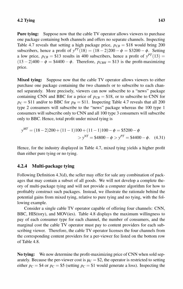
4.2 Tying 143
Pure tying: Suppose now that the cable TV operator allows viewers to purchase
one package containing both channels and offers no separate channels. Inspecting
Table 4.7 reveals that setting a high package price, pCB = $18 would bring 200
subscribers, hence a profit of yPT(18) = (18− 2)200− φ = $3200− φ . Setting
a low price, pCB = $13 results in 400 subscribers, hence a profit of yPT(13) =(13− 2)400− φ = $4400− φ . Therefore, pCBH = $13 is the profit-maximizing
price.
Mixed tying: Suppose now that the cable TV operator allows viewers to either
purchase one package containing the two channels or to subscribe to each chan-
nel separately. More precisely, viewers can now subscribe to a “news” package
containing CNN and BBC for a price of pCB = $18, or to subscribe to CNN for
pC = $11 and/or to BBC for pB = $11. Inspecting Table 4.7 reveals that all 200
type 2 consumers will subscribe to the “news” package whereas the 100 type 1
consumers will subscribe only to CNN and all 100 type 3 consumers will subscribe
only to BBC. Hence, total profit under mixed tying is
yMT = (18−2)200+(11−1)100+(11−1)100−φ = $5200−φ
> yNT = $4800−φ > yPT = $4400−φ . (4.31)
Hence, for the industry displayed in Table 4.7, mixed tying yields a higher profit
than either pure tying or no tying.
4.2.4 Multi-package tying
Following Definition 4.3(d), the seller may offer for sale any combination of pack-
ages that may contain a subset of all goods. We will not develop a complete the-
ory of multi-package tying and will not provide a computer algorithm for how to
profitably construct such packages. Instead, we illustrate the rationale behind the
potential gains from mixed tying, relative to pure tying and no tying, with the fol-
lowing example.
Consider a single cable TV operator capable of offering four channels: CNN,
BBC, HIS(tory), and MOV(ies). Table 4.8 displays the maximum willingness to
pay of each consumer type for each channel, the number of consumers, and the
marginal cost the cable TV operator must pay to content providers for each sub-
scribing viewer. Therefore, the cable TV operator licenses the four channels from
the corresponding content providers for a per-viewer fee listed on the bottom row
of Table 4.8.
No tying: We now determine the profit-maximizing price of CNN when sold sep-
arately. Because the per-viewer cost is μC = $2, the operator is restricted to setting
either pC = $4 or pC = $5 (setting pC = $1 would generate a loss). Inspecting the
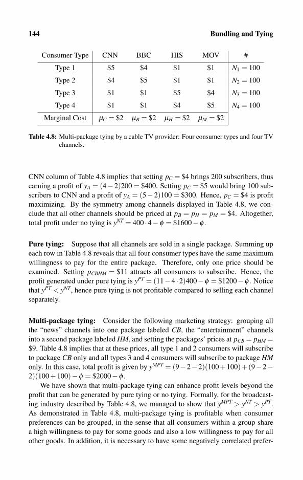
144 Bundling and Tying
Consumer Type CNN BBC HIS MOV #
Type 1 $5 $4 $1 $1 N1 = 100
Type 2 $4 $5 $1 $1 N2 = 100
Type 3 $1 $1 $5 $4 N3 = 100
Type 4 $1 $1 $4 $5 N4 = 100
Marginal Cost μC = $2 μB = $2 μH = $2 μM = $2
Table 4.8: Multi-package tying by a cable TV provider: Four consumer types and four TV
channels.
CNN column of Table 4.8 implies that setting pC = $4 brings 200 subscribers, thus
earning a profit of yA = (4−2)200 = $400. Setting pC = $5 would bring 100 sub-
scribers to CNN and a profit of yA = (5−2)100 = $300. Hence, pC = $4 is profit
maximizing. By the symmetry among channels displayed in Table 4.8, we con-
clude that all other channels should be priced at pB = pH = pM = $4. Altogether,
total profit under no tying is yNT = 400 ·4−φ = $1600−φ .
Pure tying: Suppose that all channels are sold in a single package. Summing up
each row in Table 4.8 reveals that all four consumer types have the same maximum
willingness to pay for the entire package. Therefore, only one price should be
examined. Setting pCBHM = $11 attracts all consumers to subscribe. Hence, the
profit generated under pure tying is yPT = (11−4 ·2)400−φ = $1200−φ . Notice
that yPT < yNT, hence pure tying is not profitable compared to selling each channel
separately.
Multi-package tying: Consider the following marketing strategy: grouping all
the “news” channels into one package labeled CB, the “entertainment” channels
into a second package labeled HM, and setting the packages’ prices at pCB = pHM =$9. Table 4.8 implies that at these prices, all type 1 and 2 consumers will subscribe
to package CB only and all types 3 and 4 consumers will subscribe to package HMonly. In this case, total profit is given by yMPT = (9−2−2)(100+100)+(9−2−2)(100+100)−φ = $2000−φ .
We have shown that multi-package tying can enhance profit levels beyond the
profit that can be generated by pure tying or no tying. Formally, for the broadcast-
ing industry described by Table 4.8, we managed to show that yMPT > yNT > yPT.
As demonstrated in Table 4.8, multi-package tying is profitable when consumer
preferences can be grouped, in the sense that all consumers within a group share
a high willingness to pay for some goods and also a low willingness to pay for all
other goods. In addition, it is necessary to have some negatively correlated prefer-
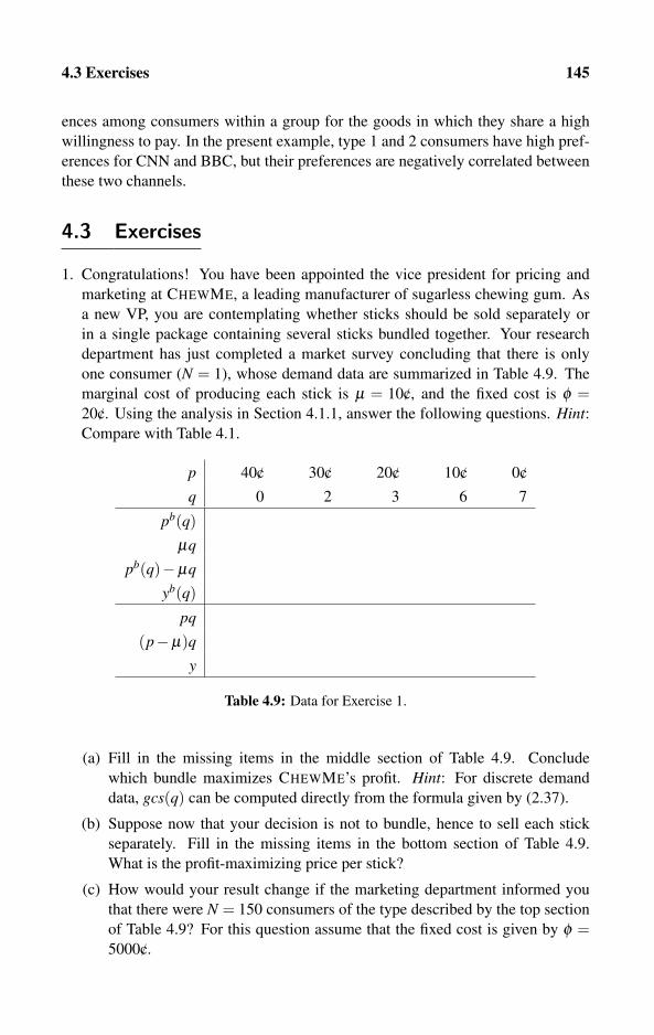
4.3 Exercises 145
ences among consumers within a group for the goods in which they share a high
willingness to pay. In the present example, type 1 and 2 consumers have high pref-
erences for CNN and BBC, but their preferences are negatively correlated between
these two channels.
4.3 Exercises
1. Congratulations! You have been appointed the vice president for pricing and
marketing at CHEWME, a leading manufacturer of sugarless chewing gum. As
a new VP, you are contemplating whether sticks should be sold separately or
in a single package containing several sticks bundled together. Your research
department has just completed a market survey concluding that there is only
one consumer (N = 1), whose demand data are summarized in Table 4.9. The
marginal cost of producing each stick is μ = 10/c, and the fixed cost is φ =20/c. Using the analysis in Section 4.1.1, answer the following questions. Hint:Compare with Table 4.1.
p 40/c 30/c 20/c 10/c 0/c
q 0 2 3 6 7
pb(q)μq
pb(q)−μq
yb(q)
pq
(p−μ)qy
Table 4.9: Data for Exercise 1.
(a) Fill in the missing items in the middle section of Table 4.9. Conclude
which bundle maximizes CHEWME’s profit. Hint: For discrete demand
data, gcs(q) can be computed directly from the formula given by (2.37).
(b) Suppose now that your decision is not to bundle, hence to sell each stick
separately. Fill in the missing items in the bottom section of Table 4.9.
What is the profit-maximizing price per stick?
(c) How would your result change if the marketing department informed you
that there were N = 150 consumers of the type described by the top section
of Table 4.9? For this question assume that the fixed cost is given by φ =5000/c.

146 Bundling and Tying
2. In the market where your firm is selling, the demand function by each individual
is approximated by a linear function given by p = 120− 0.5q. The marginal
production cost is μ = $40. Solve the following problems.
(a) Similar to Figure 4.2, draw the demand curve and compute which bundle
maximizes your firm’s profit, and what the price should be for this bundle.
(b) Suppose now that there are N = 5 consumers with the same demand func-
tion. Compute the profit level, assuming that the fixed cost is φ = $30,000.
3. Suppose that your CHEWME firm (again, a leader in the production of chewing
gum) sells to two types of consumers. The inverse demand function of a type 1
consumer is p = 8−2q and of a type 2 consumer, p = 4−q. Solve the following
problems.
(a) Write down the gross consumer surplus of each consumer type as a function
of the bundle size q. Hint: The general formulation of gcs1(q) and gcs2(q)for linear demand functions is given by (4.3). A specific example is given
in (4.10).
(b) Fill in the missing parts in Table 4.10 assuming that there are N1 = 2 type 1
consumers, there are N2 = 6 type 2 consumers, the marginal production cost
is μ = 2/c, and there are no fixed costs, φ = 0. Hint: Compare with Table 4.3.
q (bundle size) 1 2 3 4
gcs1(q)y1(q)
gcs2(q)y2(q)
min{gcs1,gcs2}y1,2(q)
max{y1,y2,y1,2}
Table 4.10: Data for Exercise 3.
(c) Conclude what the size of the bundle should be (number of units in the
bundle) to maximize the seller’s profit. Also find the profit-maximizing
price of this bundle and the number of consumers who buy it.
4. The analysis of multi-package bundling in Section 4.1.4 demonstrates the pos-
sible gains from offering two bundles for sale (rather than only one) when there
is more than one type of consumer. Suppose again that there is one consumer
of each type characterized by the two demand functions (4.9). Find two bundles

4.3 Exercises 147
〈qA, pbA〉 and 〈qB, pb
B〉 (or modify the ones given in Section 4.1.4) that also sat-
isfy condition (4.13) but generate a higher profit than the profit level computed
in (4.15). Hint: Notice that equation (4.14) implies that more surplus can be
extracted from one type of consumer.
5. Congratulations! You have been appointed the general manager of the PAR-
ADISE Hotel, which is the only hotel on Paradise Island, located somewhere in
the Pacific Ocean. This hotel also owns the only restaurant in town that serves
breakfast. As the hotel manager, your first responsibility is to decide whether
to include breakfast in the standard hotel rate or to charge extra for breakfast.
Table 4.11 shows the willingness to pay of type 1 and type 2 hotel guests for
hotel room (R) and for breakfast (B), as well as the expected number of guests
of each type and the hotel’s marginal cost of providing each service.
Guest Type Hotel Room (R) Breakfast (B) Expected # guests
Type 1 $100 $5 200
Type 2 $60 $10 800
Marginal Cost μR = $40 μB = $2
Table 4.11: Data for Exercise 5.
Solve the following problems using the single-package pure-tying analysis of
Section 4.2.1, assuming that there are no fixed costs, so φ = 0.
(a) Compute the hotel’s profit-maximizing room rate pR, breakfast price pB,
and resulting profit yNT, given that both services are sold separately (untied).
(b) Suppose now that the hotel rents a room together with breakfast. Com-
pute the package’s profit-maximizing price pRB and the corresponding profit
level yPT. Conclude whether the hotel should tie the two services in a single
package or sell them separately.
(c) Solve part (a) assuming that the expected number of type 2 guests falls
from 800 to N2 = 200 guests, whereas the expected number of type 1 guests
remains N1 = 200.
(d) Solve part (b) under the modification made in part (c).
6. Suppose now that the PARADISE Hotel, described in Exercise 5, has invested in
building a state-of-the-art gym containing a swimming pool and a sauna. The
problem facing the manager is whether to tie breakfast and a visit to the gym
with the room rental (pure tying) or whether to sell the three services sepa-
rately (no tying). The guests’ willingness to pay for each service and the hotel’s
marginal cost of providing each service are given in Table 4.12. Solve the fol-
lowing problems assuming that there are no fixed costs, so φ = 0.

148 Bundling and Tying
Type Room (R) Breakfast (B) Gym (G) # Guests
Type 1 $100 $5 $10 200
Type 2 $60 $10 $10 800
Marginal Cost μR = $40 μB = $2 μG = $0
Table 4.12: Data for Exercise 6.
(a) Compute the hotel’s profit-maximizing room rate pR, breakfast price pB,
gym entrance fee pG, and resulting profit yNT, given that each service is sold
separately (no tying).
(b) Suppose now that the hotel sells all three services in one package (pure
tying). Compute the package’s profit-maximizing price pRBG and the corre-
sponding profit level yPT. Conclude whether the hotel should tie the three
services in a single package or sell them separately.
7. Suppose now that the PARADISE Hotel offers room rentals and dinner only, and
that the guests’ willingness to pay is given by Table 4.13 below.
Guest Type Hotel Room (R) Dinner (D) Expected # Guests
Type 1 $50 $0 100
Type 2 $40 $40 100
Type 3 $0 $50 100
Marginal Cost μR = $10 μD = $10
Table 4.13: Data for Exercise 7.
Solve the following problems using the analysis of mixed tying given in Sec-
tion 4.2.3. Assume that there are no fixed costs, so φ = 0.
(a) Compute the hotel’s profit-maximizing room rate pR, dinner price pD, and
resulting profit yNT, given that both services are sold separately (no tying).
(b) Suppose now that the hotel rents a room together with dinner (pure tying).
Compute the package’s profit-maximizing price pRD and the corresponding
profit level yPT. Conclude whether the hotel should tie the two services in a
single package or sell them separately.
(c) Can a mixed tying marketing strategy enhance the hotel’s profit beyond the
profit levels achievable under no tying and pure tying? Prove your answer
by writing down the precise packages to be offered and the corresponding
prices.

4.3 Exercises 149
8. Consider a cable TV operator facing viewers and unit costs described in Table
4.14.
Consumer Type CNN BBC HIS # Subscribers
Type 1 $11 $2 $3 N1 = 100
Type 2 $11 $2 $6 N2 = 100
Type 3 $2 $11 $3 N3 = 100
Type 4 $2 $11 $6 N4 = 100
Marginal Cost μC = $1 μB = $1 μH = $1
Table 4.14: Data for Exercise 8.
Solve the following problems using the analysis of multi-package tying given in
Section 4.2.4. Assume there are no fixed costs, so φ = 0.
(a) Compute the operator’s profit-maximizing subscription rates pC, pB, and pH
and the resulting profit yNT, given that each channel is sold separately (no
tying).
(b) Compute the profit-maximizing subscription rate pCBH and the correspond-
ing profit level yPT, assuming that the operator offers only subscriptions for
a single package composed of all three channels (pure tying).
(c) Can you find alternative packages that would generate a higher profit than
that achieved by pure tying and no tying?

Chapter 5
Multipart Tariff
5.1 Two-part Tariff with One Type of Consumer 1525.1.1 Single consumer type with linear demand: An example
5.1.2 Single type with linear demand: General formulation
5.1.3 One consumer with discrete demand
5.1.4 Discrete demand with many consumers: Computer algorithm
5.2 Two-part Tariff with Multiple Consumer Types 1595.2.1 Two consumer types: An example
5.2.2 Computer algorithm for multiple consumer types
5.3 Menu of Two-part Tariffs 1655.3.1 Menu of two two-part tariffs
5.3.2 Menu of multiple two-part tariffs
5.4 Multipart Tariff 1715.4.1 Example and general formulation
5.4.2 Multipart versus a menu of two parts: Equivalence results
5.5 Regulated Public Utility 1765.6 Exercises 178
Multipart tariffs constitute another widely practiced technique of nonlinear pricing,
under which the price of each unit may vary with the total number of units pur-
chased. To some degree, multipart tariffs can be viewed as an enhancement of the
bundling marketing strategy analyzed earlier in Section 4.1. By an enhancement
we mean that instead of limiting the pricing strategy to a fixed price for a certain
number of goods bundled together in a single package, multipart tariffs consist of
a fixed fee and per-unit prices that may vary with the amount consumed.
Multipart tariffs in general, and two-part tariffs in particular, are widely used.
Here is a list of examples with which the reader should be familiar:
• Phone companies generally charge a fixed monthly fee for maintaining a line
connection and in addition charge for each minute of each phone call.
152 Multipart Tariff
• Credit card companies charge merchants and often consumers fixed annual
fees in additional to per-transaction fees.
• Membership discount retailers, such as shopping clubs, require paying an
annual membership fee before consumers are allowed to enter the store (and
then pay separately for each item they actually buy).
• Bars and nightclubs tend to collect a “cover” charge in addition to charging
for each drink separately.
• Amusement parks tend to charge an entrance fee in addition to charging for
each ride separately.
• Cellular phone operators in the United States offer consumers a menu of
different tariffs. For example, consumers get to choose from paying $30 for
the first 300 minutes plus 40/c for each additional minute, paying $50 for 600
minutes and 20/c for each additional minute, or paying $60 for the first 1000
minutes and 10/c for each additional minute.
In the literature, Coase (1946) and Gabor (1955) provide early analyses of
profit-maximizing two-part tariff structures. Oi (1971) is considered to be a pio-
neering paper on two-part tariffs. Littlechild (1975) and Mitchell (1978) extend
the analysis to capture consumption externalities (such as in telecommunications).
Schmalensee (1981) provides a comprehensive analysis of profit-maximizing two-
part tariffs for multiple consumer types, whereas Feldstein (1972), Ng and Weisser
(1974), and Willig (1978) focus mainly on tariffs that enhance social welfare. So-
cial welfare maximization as the main objective of a regulator of a public utility is
studied in Section 5.5, which also lists some textbooks on the regulation of public
utilities.
5.1 Two-part Tariff with One Type of Consumer
A two-part tariff, as the term indicates, consists of two parts: a fixed (entry) fee
and a per-unit (usage) price. The fixed fee, denoted by f , can be interpreted as the
price for purchasing the “right to enter” and buy some units of the good or service
for an additional per-unit price, denoted by p. To demonstrate it using the above
examples, an entrance fee to an amusement park that must be paid to get into the
park is the fixed part, and this fixed fee is required to be able to purchase and pay
for each ride. Similarly, membership fees (either for retail stores or for credit cards)
can be viewed as the fixed fees, which are required for obtaining the right to start
purchasing and paying on a per-unit basis.
Figure 5.1 illustrates how the revenue (which equals consumer expenditure)
extracted from a consumer varies with the consumption level q. Figure 5.1 shows
that to buy the first unit, the consumer must spend an amount of f that would then
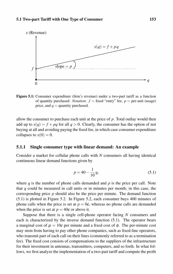
5.1 Two-part Tariff with One Type of Consumer 153
�
�
q0
x (Revenue)
f slope = p
x(q) = f + pq
•
�◦
Figure 5.1: Consumer expenditure (firm’s revenue) under a two-part tariff as a function
of quantity purchased. Notation: f = fixed “entry” fee, p = per-unit (usage)
price, and q = quantity purchased.
allow the consumer to purchase each unit at the price of p. Total outlay would then
add up to x(q) = f + pq for all q > 0. Clearly, the consumer has the option of not
buying at all and avoiding paying the fixed fee, in which case consumer expenditure
collapses to x(0) = 0.
5.1.1 Single consumer type with linear demand: An example
Consider a market for cellular phone calls with N consumers all having identical
continuous linear demand functions given by
p = 40− 1
10q, (5.1)
where q is the number of phone calls demanded and p is the price per call. Note
that q could be measured in call units or in minutes per month; in this case, the
corresponding price p should also be the price per minute. The demand function
(5.1) is plotted in Figure 5.2. In Figure 5.2, each consumer buys 400 minutes of
phone calls when the price is set at p = 0/c, whereas no phone calls are demanded
when the price is set at p = 40/c or above it.
Suppose that there is a single cell-phone operator facing N consumers and
each is characterized by the inverse demand function (5.1). The operator bears
a marginal cost of μ = 10/c per minute and a fixed cost of φ . The per-minute cost
may stem from having to pay other phone companies, such as fixed-line operators,
who transmit part of each call on their lines (commonly referred to as a termination
fee). The fixed cost consists of compensations to the suppliers of the infrastructure
for their investment in antennas, transmitters, computers, and so forth. In what fol-
lows, we first analyze the implementation of a two-part tariff and compute the profit

154 Multipart Tariff
10/c
20/c
30/c
40/c
100 200 300 400
�
p
� q (minutes)
μ
0
Area = 4500/c
Area = 3000/c
Note: gcs(300) = 4500+3000 = 7500/c
Figure 5.2: An example of a profit-maximizing two-part tariff for a single seller facing a
single consumer type with a continuous linear demand function.
generated from using this pricing strategy. Then, we compare the profit generated
from a two-part tariff to the profit generated from other pricing strategies that we
analyzed in previous chapters, that is, pure bundling and simple monopoly pricing.
Two-part tariff: The operator should choose a fixed fee f , and a per-unit price
p, that would extract maximum surplus from each consumer while leaving the con-
sumer with a nonnegative net consumer surplus. For this, we need to recall equa-
tion (2.39), which derives the gross consumer surplus for the general linear demand
function p = α−βq. Thus,
gcs(q) =(α + p)(q−0)
2=
(α +α−βq)(q−0)2
=(2α−βq)q
2. (5.2)
In the present example, (5.1) implies that α = 40 and β = −1/10. A profit-
maximizing two-part tariff can be designed using the following three steps:
Step I: Set the per-unit price to equal marginal cost, that is, p2p = μ .
Step II: From the demand function, compute the quantity demanded at this price
q2p(p2p), assuming that there is no fixed fee, that is, f = 0.
Step III: Set the fixed fee as high as possible under the constraint that each con-
sumer must gain a nonnegative net consumer surplus so that
ncs(q2p) = gcs(q2p)−q2p · p2p− f ≥ 0. (5.3)
That is, in Step III the firm raises its fixed fee component of the price to the maxi-
mum level beyond which any level would generate a negative net consumer surplus
(see Definition 2.5).
5.1 Two-part Tariff with One Type of Consumer 155
Starting with Step I, we set the per-unit price at p2p = μ = 10/c. Proceeding to
Stage II, substituting into the inverse demand function (5.1), or simply by looking
at Figure 5.2, yields a quantity demanded of q2p(10/c) = 300 phone calls. Finally,
moving to Step III, substituting q2p(10/c) = 300 into (5.2), yields a gross consumer
surplus of gcs(300) = (2 ·40−300/10)300/2 = 7500. Therefore, what is left is to
compute the highest fixed fee f that solves
ncs(300,4500,10) = 7500−300 ·10− f ≥ 0, yielding f 2p = 4500/c. (5.4)
Finally, the profit of this cell-phone operator under the two-part tariff f 2p =4500/c and p2p = 10/c can be computed as
y2p = N[
f +(p2p−μ)q2p]−φ = 4,500N−φ , (5.5)
where N is the number of consumes having the demand function (5.1) and φ is the
operator’s fixed cost.
Bundling: Section 4.1.1 analyzes single-package bundling. We now compute the
maximum profit that can be generated by using pure bundling rather than a two-part
tariff. The seller’s problem now is to bundle qb phone calls in a single package and
offer it to consumers on a take-it-or-leave-it basis. Section 4.1.1 has shown that
for the continuous linear demand case, the bundle size is determined at the point
where the inverse demand function intersects the marginal cost μ (see Figure 4.2).
Therefore, in view of Figure 5.2, the profit-maximizing bundle size is qb = 300
phone calls. Hence, the maximum price that can be charged for this bundle is
pb = gcs(300) = (2 ·40−300/10)300/2 = 7500/c. Thus, the profit from bundling
is given by
yb = N [7500−300μ]−φ = 4500N−φ = y2p, (5.6)
which is the maximum profit that can be obtained under the two-part tariff. There-
fore, for the case of identical consumers with a common demand function, a two-
part tariff is not more profitable than single-package bundling. In fact, what we have
demonstrated here is that the profit-maximizing bundling strategy can be duplicated
(that is, yields the same profit level) by an appropriate two-part tariff scheme.
Simple monopoly pricing: We now demonstrate the profit gain via the use of a
two-part tariff relative to the monopoly profit obtainable when the seller is restricted
to levying only a per-unit price (also called linear pricing). Section 3.1.2, equations
(3.2), (3.3), and (3.4) have shown that the monopoly profit-maximizing price is
pm = (α + μ)/2 = (40 + 10)/2 = 25/c. Therefore, at this price consumers make
qm = (α−μ)/(2β ) = (40−10)/(2/10) = 150 phone calls, and the seller earns
ym = N [(pm−μ)qm]−φ = 2250N−φ < y2p. (5.7)
In fact, if the seller’s fixed cost is ignored by setting φ = 0, the single seller earns
twice the amount of profit when using a two-part tariff compared with using simple
monopoly pricing. Formally, if φ = 0, ym = y2p/2.
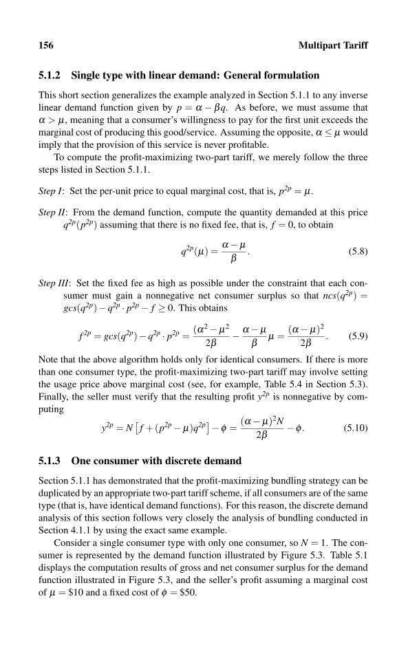
156 Multipart Tariff
5.1.2 Single type with linear demand: General formulation
This short section generalizes the example analyzed in Section 5.1.1 to any inverse
linear demand function given by p = α − βq. As before, we must assume that
α > μ , meaning that a consumer’s willingness to pay for the first unit exceeds the
marginal cost of producing this good/service. Assuming the opposite, α ≤ μ would
imply that the provision of this service is never profitable.
To compute the profit-maximizing two-part tariff, we merely follow the three
steps listed in Section 5.1.1.
Step I: Set the per-unit price to equal marginal cost, that is, p2p = μ .
Step II: From the demand function, compute the quantity demanded at this price
q2p(p2p) assuming that there is no fixed fee, that is, f = 0, to obtain
q2p(μ) =α−μ
β. (5.8)
Step III: Set the fixed fee as high as possible under the constraint that each con-
sumer must gain a nonnegative net consumer surplus so that ncs(q2p) =gcs(q2p)−q2p · p2p− f ≥ 0. This obtains
f 2p = gcs(q2p)−q2p · p2p =(α2−μ2
2β− α−μ
βμ =
(α−μ)2
2β. (5.9)
Note that the above algorithm holds only for identical consumers. If there is more
than one consumer type, the profit-maximizing two-part tariff may involve setting
the usage price above marginal cost (see, for example, Table 5.4 in Section 5.3).
Finally, the seller must verify that the resulting profit y2p is nonnegative by com-
puting
y2p = N[
f +(p2p−μ)q2p]−φ =(α−μ)2N
2β−φ . (5.10)
5.1.3 One consumer with discrete demand
Section 5.1.1 has demonstrated that the profit-maximizing bundling strategy can be
duplicated by an appropriate two-part tariff scheme, if all consumers are of the same
type (that is, have identical demand functions). For this reason, the discrete demand
analysis of this section follows very closely the analysis of bundling conducted in
Section 4.1.1 by using the exact same example.
Consider a single consumer type with only one consumer, so N = 1. The con-
sumer is represented by the demand function illustrated by Figure 5.3. Table 5.1
displays the computation results of gross and net consumer surplus for the demand
function illustrated in Figure 5.3, and the seller’s profit assuming a marginal cost
of μ = $10 and a fixed cost of φ = $50.

5.1 Two-part Tariff with One Type of Consumer 157
�
�
p
•$30
$25
••
$20
$15
μ = $10
2 6 7 93 4 5 81
••
•
$35•
q
f =gcs(7)−7p
7 · p2p
Figure 5.3: Fixed fee under a two-part tariff for a single consumer type. Note: Surplus is
computed for the case in which p2p = $15.
p $35 $30 $25 $20 $15 $10 $5
q 0 2 3 6 7 7.5 8
gcs(q) $0 $65 $92.5 $160 $177.5 $183.75 $187.5
pq $0 $60 $75.0 $120 $105.0 $75.00 $40.0
f = gcs− pq $0 $5 $17.5 $40 $72.5 $108.75 $147.5
μq $0 $20 $30.0 $60 $70.0 $75.00 $80.0
y2p −$50 −$5 −$12.5 $50 $57.5 $58.75 $57.5
Table 5.1: Two-part tariff: Single consumer type with discrete demand. Note: Computa-
tions rely on a marginal cost of μ = $10, a fixed cost of φ = $50, one consumer
N = 1, where gcs(q) is computed by (2.37).
Recall that Step I from the previous section indicates that the per-unit price
should be set to equal marginal cost μ . However, assuming that the good in question
is indivisible so the consumer must purchase whole units, Figure 5.3 shows that
setting p = μ = $10 would induce the consumer to buy only six units and that
the same quantity demanded is obtainable also by setting p = $15 > μ , which is a
higher price.
Table 5.1 computes the gross consumer surplus gcs(q) for each quantity de-
manded q. Readers who wish to learn about these computations are referred to
Table 2.5, which uses the same demand data. Similar to Step III for the continuous
demand case, the fixed fee f is computed by the constraint that consumers do not
buy products and services unless they gain nonnegative net consumer surplus, that
is, ncs(q) = gcs(q)− pq− f ≥ 0, which is listed on the fifth row in Table 5.1. Ta-
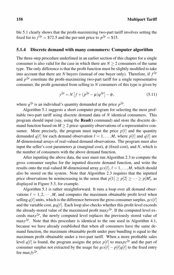
158 Multipart Tariff
ble 5.1 clearly shows that the profit-maximizing two-part tariff involves setting the
fixed fee to f 2p = $72.5 and the per-unit price to p2p = $15.
5.1.4 Discrete demand with many consumers: Computer algorithm
The three-step procedure underlined in an earlier section of this chapter for a single
consumer is also valid for the case in which there are N ≥ 2 consumers of the same
type. The only difference is that the profit function must be slightly modified to take
into account that there are N buyers (instead of one buyer only). Therefore, if f 2p
and p2p constitute the profit-maximizing two-part tariff for a single representative
consumer, the profit generated from selling to N consumers of this type is given by
y2p = N[
f +(p2p−μ)q2p]−φ , (5.11)
where q2p is an individual’s quantity demanded at the price p2p.
Algorithm 5.1 suggests a short computer program for selecting the most prof-
itable two-part tariff using discrete demand data of N identical consumers. This
program should input (say, using the Read() command) and store the discrete de-
mand function based on M ≥ 2 price–quantity observations of a representative con-
sumer. More precisely, the program must input the price p[�] and the quantity
demanded q[�] for each demand observation � = 1, . . . ,M, where p[�] and q[�] are
M-dimensional arrays of real-valued demand observations. The program must also
input the seller’s cost parameters μ (marginal cost), φ (fixed cost), and N, which is
the number of consumers with the above demand function.
After inputting the above data, the user must run Algorithm 2.3 to compute the
gross consumer surplus for the inputted discrete demand function, and write the
results onto the real-valued M-dimensional array gcs[�], � = 1, . . . ,M, which should
also be stored on the system. Note that Algorithm 2.3 requires that the inputted
price observations be nonincreasing in the sense that p[1] ≥ p[2] ≥ ·· · ≥ p[M], as
displayed in Figure 5.3, for example.
Algorithm 5.1 is rather straightforward. It runs a loop over all demand obser-
vations � = 1,2, · · · ,M, and computes the maximum obtainable profit level when
selling q[�] units, which is the difference between the gross consumer surplus, gcs[�]and the variable cost, μq[�]. Each loop also checks whether this profit level exceeds
the already-stored value of the maximized profit maxy2p. If the computed level ex-
ceeds maxy2p, the newly computed level replaces the previously stored value of
maxy2p. Note that this procedure is identical to the one used in Algorithm 4.1,
because we have already established that when all consumers have the same de-
mand function, the maximum obtainable profit under pure bundling is equal to the
maximum profit obtainable under a two-part tariff. When a more profitable sales
level q[�] is found, the program assigns the price p[�] to maxpy2p and the part of
consumer surplus not extracted by the usage fee gcs[�]− p[�]q[�] to the fixed entry
fee max fy2p.
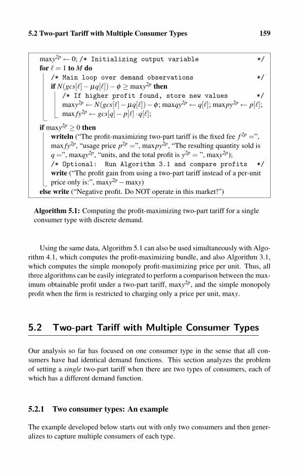
5.2 Two-part Tariff with Multiple Consumer Types 159
maxy2p← 0; /* Initializing output variable */for � = 1 to M do
/* Main loop over demand observations */if N(gcs[�]−μq[�])−φ ≥maxy2p then
/* If higher profit found, store new values */maxy2p← N(gcs[�]−μq[�])−φ ; maxqy2p← q[�]; maxpy2p← p[�];max fy2p← gcs[q]− p[�] ·q[�];
if maxy2p ≥ 0 thenwriteln (“The profit-maximizing two-part tariff is the fixed fee f 2p =”,
max fy2p, “usage price p2p =”, maxpy2p, “The resulting quantity sold is
q =”, maxqy2p, “units, and the total profit is y2p = ”, maxy2p);
/* Optional: Run Algorithm 3.1 and compare profits */write (“The profit gain from using a two-part tariff instead of a per-unit
price only is:”, maxy2p−maxy)
else write (“Negative profit. Do NOT operate in this market!”)
Algorithm 5.1: Computing the profit-maximizing two-part tariff for a single
consumer type with discrete demand.
Using the same data, Algorithm 5.1 can also be used simultaneously with Algo-
rithm 4.1, which computes the profit-maximizing bundle, and also Algorithm 3.1,
which computes the simple monopoly profit-maximizing price per unit. Thus, all
three algorithms can be easily integrated to perform a comparison between the max-
imum obtainable profit under a two-part tariff, maxy2p, and the simple monopoly
profit when the firm is restricted to charging only a price per unit, maxy.
5.2 Two-part Tariff with Multiple Consumer Types
Our analysis so far has focused on one consumer type in the sense that all con-
sumers have had identical demand functions. This section analyzes the problem
of setting a single two-part tariff when there are two types of consumers, each of
which has a different demand function.
5.2.1 Two consumer types: An example
The example developed below starts out with only two consumers and then gener-
alizes to capture multiple consumers of each type.
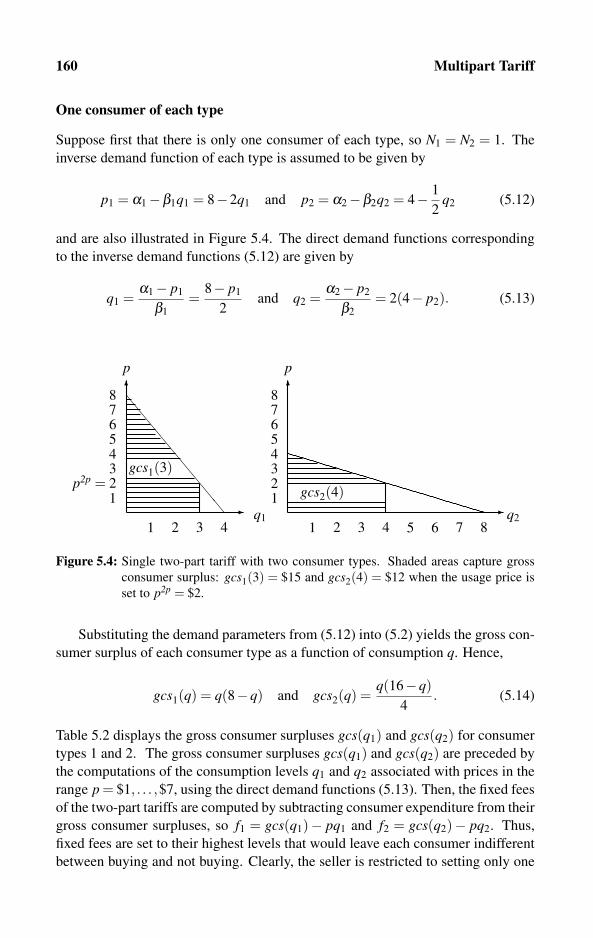
160 Multipart Tariff
One consumer of each type
Suppose first that there is only one consumer of each type, so N1 = N2 = 1. The
inverse demand function of each type is assumed to be given by
p1 = α1−β1q1 = 8−2q1 and p2 = α2−β2q2 = 4− 1
2q2 (5.12)
and are also illustrated in Figure 5.4. The direct demand functions corresponding
to the inverse demand functions (5.12) are given by
q1 =α1− p1
β1=
8− p1
2and q2 =
α2− p2
β2= 2(4− p2). (5.13)
2
1p2p = 2
345678
1 3 4
� q12
12345678
1 3 4 5 6 7 8
� q2
� ����������
p p
gcs1(3)
gcs2(4)
Figure 5.4: Single two-part tariff with two consumer types. Shaded areas capture gross
consumer surplus: gcs1(3) = $15 and gcs2(4) = $12 when the usage price is
set to p2p = $2.
Substituting the demand parameters from (5.12) into (5.2) yields the gross con-
sumer surplus of each consumer type as a function of consumption q. Hence,
gcs1(q) = q(8−q) and gcs2(q) =q(16−q)
4. (5.14)
Table 5.2 displays the gross consumer surpluses gcs(q1) and gcs(q2) for consumer
types 1 and 2. The gross consumer surpluses gcs(q1) and gcs(q2) are preceded by
the computations of the consumption levels q1 and q2 associated with prices in the
range p = $1, . . . ,$7, using the direct demand functions (5.13). Then, the fixed fees
of the two-part tariffs are computed by subtracting consumer expenditure from their
gross consumer surpluses, so f1 = gcs(q1)− pq1 and f2 = gcs(q2)− pq2. Thus,
fixed fees are set to their highest levels that would leave each consumer indifferent
between buying and not buying. Clearly, the seller is restricted to setting only one
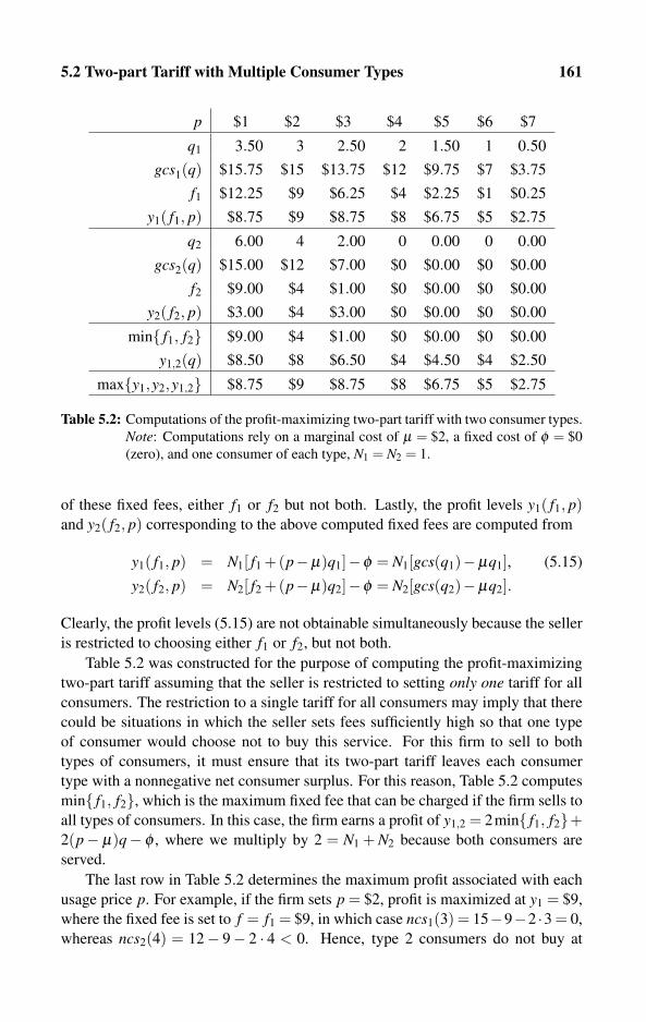
5.2 Two-part Tariff with Multiple Consumer Types 161
p $1 $2 $3 $4 $5 $6 $7
q1 3.50 3 2.50 2 1.50 1 0.50
gcs1(q) $15.75 $15 $13.75 $12 $9.75 $7 $3.75
f1 $12.25 $9 $6.25 $4 $2.25 $1 $0.25
y1( f1, p) $8.75 $9 $8.75 $8 $6.75 $5 $2.75
q2 6.00 4 2.00 0 0.00 0 0.00
gcs2(q) $15.00 $12 $7.00 $0 $0.00 $0 $0.00
f2 $9.00 $4 $1.00 $0 $0.00 $0 $0.00
y2( f2, p) $3.00 $4 $3.00 $0 $0.00 $0 $0.00
min{ f1, f2} $9.00 $4 $1.00 $0 $0.00 $0 $0.00
y1,2(q) $8.50 $8 $6.50 $4 $4.50 $4 $2.50
max{y1,y2,y1,2} $8.75 $9 $8.75 $8 $6.75 $5 $2.75
Table 5.2: Computations of the profit-maximizing two-part tariff with two consumer types.
Note: Computations rely on a marginal cost of μ = $2, a fixed cost of φ = $0
(zero), and one consumer of each type, N1 = N2 = 1.
of these fixed fees, either f1 or f2 but not both. Lastly, the profit levels y1( f1, p)and y2( f2, p) corresponding to the above computed fixed fees are computed from
y1( f1, p) = N1[ f1 +(p−μ)q1]−φ = N1[gcs(q1)−μq1], (5.15)
y2( f2, p) = N2[ f2 +(p−μ)q2]−φ = N2[gcs(q2)−μq2].
Clearly, the profit levels (5.15) are not obtainable simultaneously because the seller
is restricted to choosing either f1 or f2, but not both.
Table 5.2 was constructed for the purpose of computing the profit-maximizing
two-part tariff assuming that the seller is restricted to setting only one tariff for all
consumers. The restriction to a single tariff for all consumers may imply that there
could be situations in which the seller sets fees sufficiently high so that one type
of consumer would choose not to buy this service. For this firm to sell to both
types of consumers, it must ensure that its two-part tariff leaves each consumer
type with a nonnegative net consumer surplus. For this reason, Table 5.2 computes
min{ f1, f2}, which is the maximum fixed fee that can be charged if the firm sells to
all types of consumers. In this case, the firm earns a profit of y1,2 = 2min{ f1, f2}+2(p− μ)q− φ , where we multiply by 2 = N1 + N2 because both consumers are
served.
The last row in Table 5.2 determines the maximum profit associated with each
usage price p. For example, if the firm sets p = $2, profit is maximized at y1 = $9,
where the fixed fee is set to f = f1 = $9, in which case ncs1(3) = 15−9−2 ·3 = 0,
whereas ncs2(4) = 12− 9− 2 · 4 < 0. Hence, type 2 consumers do not buy at

162 Multipart Tariff
this tariff. Comparing all the profit levels on the bottom row of Table 5.2 reveals
that the profit-maximizing two-part tariff is f 2p = $9 and p2p = $2. As discussed
above, only type 1 consumers buy (see also Figure 5.4), and the firm earns a profit
of y(9,2) = $9.
Multiple consumers of each type
The calculation results exhibited in Table 5.2 are based on two consumer types,
defined by the demand functions (5.12) and N1 = N2 = 1 (one consumer per type).
We now extend this example to multiple consumers of each type. Formally, suppose
that there are N1 = 2 type 1 consumers and N2 = 5 type 2 consumers. Table 5.3
modifies Table 5.2 by recalculating the profit levels for each quantity demanded
associated with the price p appearing on the top of this table. The recalculated
profit levels in Table 5.3 are based on y1(q) = 2[ f1 +(p−μ)q]−φ , y2(q) = 5[ f2 +(p− μ)q)]− φ , and y1,2(q) def= (2 + 5)[ f1,2 + (p− μ)(q1 + q2)]− φ , where f1,2 =min{ f1, f2}.
p $1 $2 $3 $4 $5 $6 $7
q1 3.50 3 2.50 2 1.50 1 0.50
gcs1(q) $15.75 $15 $13.75 $12 $9.75 $7 $3.75
f1 $12.25 $9 $6.25 $4 $2.25 $1 $0.25
y1( f1, p) $17.50 $18 $17.50 $16 $13.50 $10 $5.50
q2 6.00 4 2.00 0 0.00 0 0.00
gcs2(q) $15.00 $12 $7.00 $0 $0.00 $0 $0.00
f2 $9.00 $4 $1.00 $0 $0.00 $0 $0.00
y2( f2, p) $15.00 $20 $15.00 $0 $0.00 $0 $0
min{ f1, f2} $9.00 $4 $1.00 $0 $0.00 $0 $0.00
y1,2(q) $26.00 $28 $22.00 $8 $9.00 $8 $5.00
max{y1,y2,y1,2} $26.00 $28 $22.00 $16 $13.50 $10 $5.50
Table 5.3: Extending Table 5.2 to multiple consumers, N1 = 2 and N2 = 5.
The computations exhibited in Table 5.3 reveal that the profit-maximizing us-
age price is p2p = $2, where each type 1 consumer buys q1 = 3 units and each type 2
consumer buys q2 = 4 units. However, unlike the case in which N1 = N2 = 1, here
the seller lowers the fixed fee to f 2p = $4 = min{$9,$4} so that all the 2 + 5 con-
sumers are served (both have a nonnegative gross consumer surplus). This should
come as no surprise because our assumption that there are “many” type 2 con-
sumers, N2 = 5, implies that excluding them is not profitable for this seller.
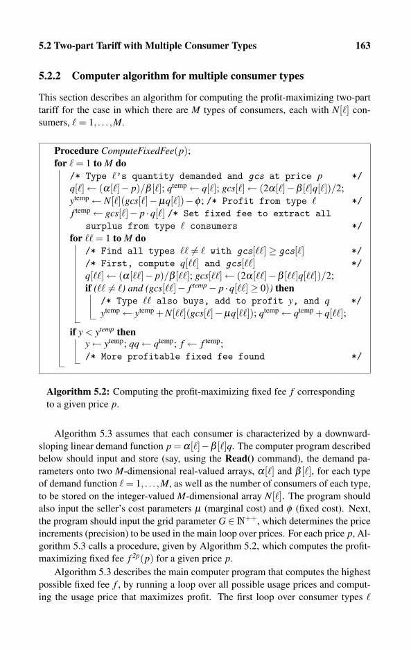
5.2 Two-part Tariff with Multiple Consumer Types 163
5.2.2 Computer algorithm for multiple consumer types
This section describes an algorithm for computing the profit-maximizing two-part
tariff for the case in which there are M types of consumers, each with N[�] con-
sumers, � = 1, . . . ,M.
Procedure ComputeFixedFee(p);for � = 1 to M do
/* Type �’s quantity demanded and gcs at price p */q[�]← (α[�]− p)/β [�]; qtemp← q[�]; gcs[�]← (2α[�]−β [�]q[�])/2;
ytemp← N[�](gcs[�]−μq[�])−φ ; /* Profit from type � */f temp← gcs[�]− p ·q[�] /* Set fixed fee to extract all
surplus from type � consumers */for �� = 1 to M do
/* Find all types �� �= � with gcs[��]≥ gcs[�] *//* First, compute q[��] and gcs[��] */q[��]← (α[��]− p)/β [��]; gcs[��]← (2α[��]−β [��]q[��])/2;
if (�� �= �) and (gcs[��]− f temp− p ·q[��]≥ 0)) then/* Type �� also buys, add to profit y, and q */ytemp← ytemp +N[��](gcs[�]−μq[��]); qtemp← qtemp +q[��];
if y < ytemp theny← ytemp; qq← qtemp; f ← f temp;
/* More profitable fixed fee found */
Algorithm 5.2: Computing the profit-maximizing fixed fee f corresponding
to a given price p.
Algorithm 5.3 assumes that each consumer is characterized by a downward-
sloping linear demand function p = α[�]−β [�]q. The computer program described
below should input and store (say, using the Read() command), the demand pa-
rameters onto two M-dimensional real-valued arrays, α[�] and β [�], for each type
of demand function � = 1, . . . ,M, as well as the number of consumers of each type,
to be stored on the integer-valued M-dimensional array N[�]. The program should
also input the seller’s cost parameters μ (marginal cost) and φ (fixed cost). Next,
the program should input the grid parameter G ∈N++, which determines the price
increments (precision) to be used in the main loop over prices. For each price p, Al-
gorithm 5.3 calls a procedure, given by Algorithm 5.2, which computes the profit-
maximizing fixed fee f 2p(p) for a given price p.
Algorithm 5.3 describes the main computer program that computes the highest
possible fixed fee f , by running a loop over all possible usage prices and comput-
ing the usage price that maximizes profit. The first loop over consumer types �

164 Multipart Tariff
y2p← 0; q2p← 0; /* Initializing output variables */pmax← 0/* Computing highest possible price */for � = 1 to M do
/* Loop over all consumer types */if pmax < α[�] then pmax← α[�]; /* Demand intercept */
p← pmax; Δp← pmax/G; /* Price increments (precision) */while p≥ 0 do
f ← 0; y← 0; qq← 0; /* Main loop over prices */Call Procedure ComputeFixedFee(p); /* Algorithm 5.2 */if y2p < y then y2p← y; p2p← p; q2p← qq; f 2p← f ;
/* Fixed fee f yields higher profit */p← p−Δp; /* Reduce price before repeating this loop */
if y2p ≥ φ thenwriteln (“The profit-maximizing two-part tariff is composed of a fixed
fee f 2p =”, f 2p, “and a usage price p2p =”, p2p);
write (“The firm sells q2p =”, q2p, “units, and the resulting total profit is
y2p = ”, y2p);
else write (“Negative profit. Do NOT operate in this market!”)
Algorithm 5.3: Computing the profit-maximizing two-part tariff for multiple
consumer types with linear demand.
determines the maximum possible price pmax beyond which no consumer will be
demanding the service. Clearly, pmax = max� α[�], which is the highest demand
intercept with the price axis. For a given price p, the procedure given by Algo-
rithm 5.2 runs a loop over all the � = 1, . . . ,M consumer types to compute the max-
imum surplus that can be extracted by adjusting the fixed fee f . For each type �,
the program sets the fixed fee to extract all the surplus, so f = gcs�− p ·q�. Then,
the internal loop checks which other types of consumers also buy the service under
f by checking whether ncs�� = gcs��− p ·q�� ≥ 0. If this is the case, the profit from
the N[��] consumers is added to the total profit. Otherwise, the N[��] consumers are
excluded from the market at this particular fixed fee f and the given price p.
The main loop runs over prices starting from pmax and ending with p = 0.
For each price p, the program calls the procedure ComputeFixedFee(p) given by
Algorithm 5.2, which computes the profit-maximizing fixed fee f , corresponding
profit y, and sales level qq. Algorithm 5.3 updates the profit y2p, the quantity sold,
q2p, and the fixed fee f 2p in the event that Algorithm 5.2 finds that the price pgenerates a higher profit.
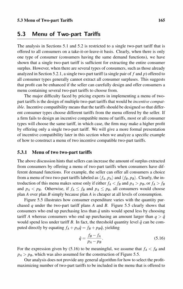
5.3 Menu of Two-part Tariffs 165
5.3 Menu of Two-part Tariffs
The analysis in Sections 5.1 and 5.2 is restricted to a single two-part tariff that is
offered to all consumers on a take-it-or-leave-it basis. Clearly, when there is only
one type of consumer (consumers having the same demand functions), we have
shown that a single two-part tariff is sufficient for extracting the entire consumer
surplus. However, when there are several types of consumers, such as those already
analyzed in Section 5.2.1, a single two-part tariff (a single pair of f and p) offered to
all consumer types generally cannot extract all consumer surpluses. This suggests
that profit can be enhanced if the seller can carefully design and offer consumers a
menu containing several two-part tariffs to choose from.
The major difficulty faced by pricing experts in implementing a menu of two-
part tariffs is the design of multiple two-part tariffs that would be incentive compat-ible. Incentive compatibility means that the tariffs should be designed so that differ-
ent consumer types choose different tariffs from the menu offered by the seller. If
a firm fails to design an incentive compatible menu of tariffs, most or all consumer
types will choose the same tariff, in which case, the firm may make a higher profit
by offering only a single two-part tariff. We will give a more formal presentation
of incentive compatibility later in this section when we analyze a specific example
of how to construct a menu of two incentive compatible two-part tariffs.
5.3.1 Menu of two two-part tariffs
The above discussion hints that sellers can increase the amount of surplus extracted
from consumers by offering a menu of two-part tariffs when consumers have dif-
ferent demand functions. For example, the seller can offer all consumers a choice
from a menu of two two-part tariffs labeled as 〈 fA, pA〉 and 〈 fB, pB〉. Clearly, the in-
troduction of this menu makes sense only if either fA < fB and pA > pB, or fA > fB
and pA < pB. Otherwise, if fA ≤ fB and pA ≤ pB, all consumers would choose
plan A over plan B simply because plan A is cheaper at all levels of consumption.
Figure 5.5 illustrates how consumer expenditure varies with the quantity pur-
chased q under the two-part tariff plans A and B. Figure 5.5 clearly shows that
consumers who end up purchasing less than q units would spend less by choosing
tariff A whereas consumers who end up purchasing an amount larger than q > qwould spend less under tariff B. In fact, the threshold quantity level q can be com-
puted directly by equating fA + pAq = fB + pBq, yielding
q =fB− fA
pA− pB. (5.16)
For the expression given by (5.16) to be meaningful, we assume that fA < fB and
pA > pB, which was also assumed for the construction of Figure 5.5.
Our analysis does not provide any general algorithm for how to select the profit-
maximizing number of two-part tariffs to be included in the menu that is offered to
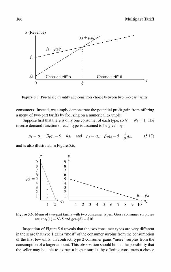
166 Multipart Tariff
�
�
q0
x (Revenue)
q
fA
fB
fB + pBq
fA + pAq
Choose tariff A Choose tariff B
Figure 5.5: Purchased quantity and consumer choice between two two-part tariffs.
consumers. Instead, we simply demonstrate the potential profit gain from offering
a menu of two-part tariffs by focusing on a numerical example.
Suppose first that there is only one consumer of each type, so N1 = N2 = 1. The
inverse demand function of each type is assumed to be given by
p1 = α1−β1q1 = 9−4q1 and p2 = α2−β2q2 = 5− 1
2q2, (5.17)
and is also illustrated in Figure 5.6.
2
1
34
pA = 5678
1
2
�
p
9
� q12
12345678
1 3 4 5 6 7 8
�
p
9
9 10
� q2
μ = pB
Figure 5.6: Menu of two-part tariffs with two consumer types. Gross consumer surpluses
are gcs1(1) = $3.5 and gcs2(8) = $16.
Inspection of Figure 5.6 reveals that the two consumer types are very different
in the sense that type 1 gains “most” of the consumer surplus from the consumption
of the first few units. In contract, type 2 consumer gains “more” surplus from the
consumption of a larger amount. This observation should hint at the possibility that
the seller may be able to extract a higher surplus by offering consumers a choice
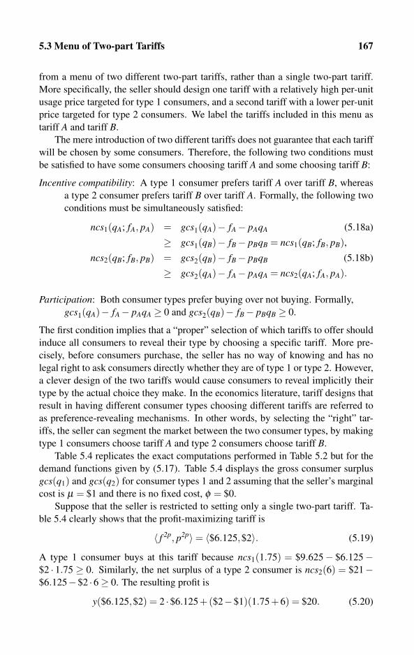
5.3 Menu of Two-part Tariffs 167
from a menu of two different two-part tariffs, rather than a single two-part tariff.
More specifically, the seller should design one tariff with a relatively high per-unit
usage price targeted for type 1 consumers, and a second tariff with a lower per-unit
price targeted for type 2 consumers. We label the tariffs included in this menu as
tariff A and tariff B.
The mere introduction of two different tariffs does not guarantee that each tariff
will be chosen by some consumers. Therefore, the following two conditions must
be satisfied to have some consumers choosing tariff A and some choosing tariff B:
Incentive compatibility: A type 1 consumer prefers tariff A over tariff B, whereas
a type 2 consumer prefers tariff B over tariff A. Formally, the following two
conditions must be simultaneously satisfied:
ncs1(qA; fA, pA) = gcs1(qA)− fA− pAqA (5.18a)
≥ gcs1(qB)− fB− pBqB = ncs1(qB; fB, pB),ncs2(qB; fB, pB) = gcs2(qB)− fB− pBqB (5.18b)
≥ gcs2(qA)− fA− pAqA = ncs2(qA; fA, pA).
Participation: Both consumer types prefer buying over not buying. Formally,
gcs1(qA)− fA− pAqA ≥ 0 and gcs2(qB)− fB− pBqB ≥ 0.
The first condition implies that a “proper” selection of which tariffs to offer should
induce all consumers to reveal their type by choosing a specific tariff. More pre-
cisely, before consumers purchase, the seller has no way of knowing and has no
legal right to ask consumers directly whether they are of type 1 or type 2. However,
a clever design of the two tariffs would cause consumers to reveal implicitly their
type by the actual choice they make. In the economics literature, tariff designs that
result in having different consumer types choosing different tariffs are referred to
as preference-revealing mechanisms. In other words, by selecting the “right” tar-
iffs, the seller can segment the market between the two consumer types, by making
type 1 consumers choose tariff A and type 2 consumers choose tariff B.
Table 5.4 replicates the exact computations performed in Table 5.2 but for the
demand functions given by (5.17). Table 5.4 displays the gross consumer surplus
gcs(q1) and gcs(q2) for consumer types 1 and 2 assuming that the seller’s marginal
cost is μ = $1 and there is no fixed cost, φ = $0.
Suppose that the seller is restricted to setting only a single two-part tariff. Ta-
ble 5.4 clearly shows that the profit-maximizing tariff is
〈 f 2p, p2p〉= 〈$6.125,$2〉. (5.19)
A type 1 consumer buys at this tariff because ncs1(1.75) = $9.625− $6.125−$2 · 1.75 ≥ 0. Similarly, the net surplus of a type 2 consumer is ncs2(6) = $21−$6.125−$2 ·6≥ 0. The resulting profit is
y($6.125,$2) = 2 ·$6.125+($2−$1)(1.75+6) = $20. (5.20)
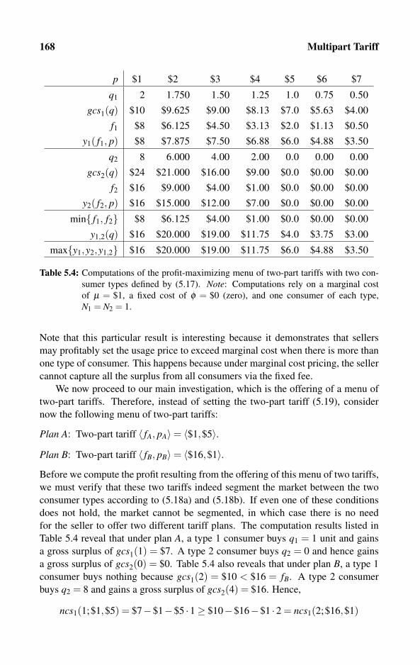
168 Multipart Tariff
p $1 $2 $3 $4 $5 $6 $7
q1 2 1.750 1.50 1.25 1.0 0.75 0.50
gcs1(q) $10 $9.625 $9.00 $8.13 $7.0 $5.63 $4.00
f1 $8 $6.125 $4.50 $3.13 $2.0 $1.13 $0.50
y1( f1, p) $8 $7.875 $7.50 $6.88 $6.0 $4.88 $3.50
q2 8 6.000 4.00 2.00 0.0 0.00 0.00
gcs2(q) $24 $21.000 $16.00 $9.00 $0.0 $0.00 $0.00
f2 $16 $9.000 $4.00 $1.00 $0.0 $0.00 $0.00
y2( f2, p) $16 $15.000 $12.00 $7.00 $0.0 $0.00 $0.00
min{ f1, f2} $8 $6.125 $4.00 $1.00 $0.0 $0.00 $0.00
y1,2(q) $16 $20.000 $19.00 $11.75 $4.0 $3.75 $3.00
max{y1,y2,y1,2} $16 $20.000 $19.00 $11.75 $6.0 $4.88 $3.50
Table 5.4: Computations of the profit-maximizing menu of two-part tariffs with two con-
sumer types defined by (5.17). Note: Computations rely on a marginal cost
of μ = $1, a fixed cost of φ = $0 (zero), and one consumer of each type,
N1 = N2 = 1.
Note that this particular result is interesting because it demonstrates that sellers
may profitably set the usage price to exceed marginal cost when there is more than
one type of consumer. This happens because under marginal cost pricing, the seller
cannot capture all the surplus from all consumers via the fixed fee.
We now proceed to our main investigation, which is the offering of a menu of
two-part tariffs. Therefore, instead of setting the two-part tariff (5.19), consider
now the following menu of two-part tariffs:
Plan A: Two-part tariff 〈 fA, pA〉= 〈$1,$5〉.Plan B: Two-part tariff 〈 fB, pB〉= 〈$16,$1〉.Before we compute the profit resulting from the offering of this menu of two tariffs,
we must verify that these two tariffs indeed segment the market between the two
consumer types according to (5.18a) and (5.18b). If even one of these conditions
does not hold, the market cannot be segmented, in which case there is no need
for the seller to offer two different tariff plans. The computation results listed in
Table 5.4 reveal that under plan A, a type 1 consumer buys q1 = 1 unit and gains
a gross surplus of gcs1(1) = $7. A type 2 consumer buys q2 = 0 and hence gains
a gross surplus of gcs2(0) = $0. Table 5.4 also reveals that under plan B, a type 1
consumer buys nothing because gcs1(2) = $10 < $16 = fB. A type 2 consumer
buys q2 = 8 and gains a gross surplus of gcs2(4) = $16. Hence,
ncs1(1;$1,$5) = $7−$1−$5 ·1≥ $10−$16−$1 ·2 = ncs1(2;$16,$1)
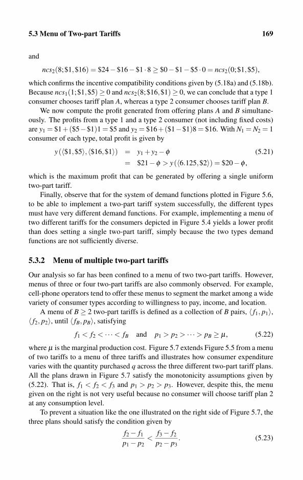
5.3 Menu of Two-part Tariffs 169
and
ncs2(8;$1,$16) = $24−$16−$1 ·8≥ $0−$1−$5 ·0 = ncs2(0;$1,$5),
which confirms the incentive compatibility conditions given by (5.18a) and (5.18b).
Because ncs1(1;$1,$5)≥ 0 and ncs2(8;$16,$1)≥ 0, we can conclude that a type 1
consumer chooses tariff plan A, whereas a type 2 consumer chooses tariff plan B.
We now compute the profit generated from offering plans A and B simultane-
ously. The profits from a type 1 and a type 2 consumer (not including fixed costs)
are y1 = $1+($5−$1)1 = $5 and y2 = $16+($1−$1)8 = $16. With N1 = N2 = 1
consumer of each type, total profit is given by
y(〈$1,$5〉,〈$16,$1〉) = y1 + y2−φ (5.21)
= $21−φ > y(〈6.125,$2〉) = $20−φ ,
which is the maximum profit that can be generated by offering a single uniform
two-part tariff.
Finally, observe that for the system of demand functions plotted in Figure 5.6,
to be able to implement a two-part tariff system successfully, the different types
must have very different demand functions. For example, implementing a menu of
two different tariffs for the consumers depicted in Figure 5.4 yields a lower profit
than does setting a single two-part tariff, simply because the two types demand
functions are not sufficiently diverse.
5.3.2 Menu of multiple two-part tariffs
Our analysis so far has been confined to a menu of two two-part tariffs. However,
menus of three or four two-part tariffs are also commonly observed. For example,
cell-phone operators tend to offer these menus to segment the market among a wide
variety of consumer types according to willingness to pay, income, and location.
A menu of B ≥ 2 two-part tariffs is defined as a collection of B pairs, 〈 f1, p1〉,〈 f2, p2〉, until 〈 fB, pB〉, satisfying
f1 < f2 < · · ·< fB and p1 > p2 > · · ·> pB ≥ μ , (5.22)
where μ is the marginal production cost. Figure 5.7 extends Figure 5.5 from a menu
of two tariffs to a menu of three tariffs and illustrates how consumer expenditure
varies with the quantity purchased q across the three different two-part tariff plans.
All the plans drawn in Figure 5.7 satisfy the monotonicity assumptions given by
(5.22). That is, f1 < f2 < f3 and p1 > p2 > p3. However, despite this, the menu
given on the right is not very useful because no consumer will choose tariff plan 2
at any consumption level.
To prevent a situation like the one illustrated on the right side of Figure 5.7, the
three plans should satisfy the condition given by
f2− f1
p1− p2<
f3− f2
p2− p3. (5.23)

170 Multipart Tariff
�
0
x (Revenue)
f1 � q
f2
f3
�
0
x (Revenue)
f1 � qq1,2 q2,3
21 Choose Plan 3
Choose�����������
f2
f3
q1,3
Choose Plan 31
Figure 5.7: Left: Implementable menu of three two-part tariffs. Right: Poorly adminis-
tered menu of three two-part tariffs.
To prove condition (5.23), observe that the cutoff quantities q1,2 and q2,3 plotted in
Figure 5.7 are determined by solving f1 + p1q1,2 = f2 + p2q1,2 and f2 + p2q2,3 =f3 + p3q2,3, respectively. Hence,
q1,2 =f2− f1
p1− p2<
f3− f2
p2− p3= q2,3, (5.24)
as long as condition (5.23) holds.
We summarize our discussion of menus of multiple two-part tariffs by listing
some guidelines that are necessary (but not sufficient) for making a menu contain-
ing B two-part tariffs (5.22) implementable, useful, and profitable.
Menu size: The number of tariffs in the menu should not exceed the number of
consumer types. Formally, B≤M.
Monotone crossing: Similar to condition (5.23),
f2− f1
p1− p2<
f3− f2
p2− p3< · · ·< fB− fB−1
pB−1− pB. (5.25)
Incentive compatibility: Each tariff should be adopted by at least one type of con-
sumer. Formally, let plans i and j be on the menu. Then, there must exist
type � consumers for which ncs�(q�(pi); fi, pi) ≥ ncs�(q�(p j); f j, p j). That
is, type � consumers prefer plan i over all other plans on this menu.
Participation: For each plan i on the menu, i = 1, . . . ,B, there exists a consumer
type � for which ncs�(q�(pi); fi, pi)≥ 0.
Relative Profitability: The offering of this menu of two-part tariffs should be more
profitable than offering a single two-part tariff.
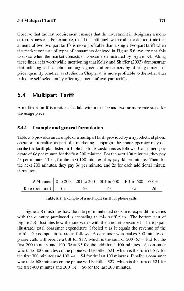
5.4 Multipart Tariff 171
Observe that the last requirement ensures that the investment in designing a menu
of tariffs pays off. For example, recall that although we are able to demonstrate that
a menu of two two-part tariffs is more profitable than a single two-part tariff when
the market consists of types of consumers depicted in Figure 5.6, we are not able
to do so when the market consists of consumers illustrated by Figure 5.4. Along
these lines, it is worthwhile mentioning that Kolay and Shaffer (2003) demonstrate
that inducing self-selection among segments of consumers by offering a menu of
price–quantity bundles, as studied in Chapter 4, is more profitable to the seller than
inducing self-selection by offering a menu of two-part tariffs.
5.4 Multipart Tariff
A multipart tariff is a price schedule with a flat fee and two or more rate steps for
the usage price.
5.4.1 Example and general formulation
Table 5.5 provides an example of a multipart tariff provided by a hypothetical phone
operator. In reality, as part of a marketing campaign, the phone operator may de-
scribe the tariff plan listed in Table 5.5 to its customers as follows: Consumers pay
a rate of 6/c per minute for the first 200 minutes. For the next 100 minutes, they pay
5/c per minute. Then, for the next 100 minutes, they pay 4/c per minute. Then, for
the next 200 minutes, they pay 3/c per minute, and 2/c for each additional minute
thereafter.
# Minutes 0 to 200 201 to 300 301 to 400 401 to 600 601+
Rate (per min.) 6/c 5/c 4/c 3/c 2/c
Table 5.5: Example of a multipart tariff for phone calls.
Figure 5.8 illustrates how the rate per minute and consumer expenditure varies
with the quantity purchased q according to this tariff plan. The bottom part of
Figure 5.8 illustrates how the rate varies with the amount consumed. The top part
illustrates total consumer expenditure (labeled x as it equals the revenue of the
firm). The computations are as follows: A consumer who makes 300 minutes of
phone calls will receive a bill for $17, which is the sum of 200 · 6/c = $12 for the
first 200 minutes and 100 · 5/c = $5 for the additional 100 minutes. A consumer
who talks 400 minutes on the phone will be billed $21, which is the sum of $17 for
the first 300 minutes and 100 ·4/c = $4 for the last 100 minutes. Finally, a consumer
who talks 600 minutes on the phone will be billed $27, which is the sum of $21 for
the first 400 minutes and 200 ·3/c = $6 for the last 200 minutes.
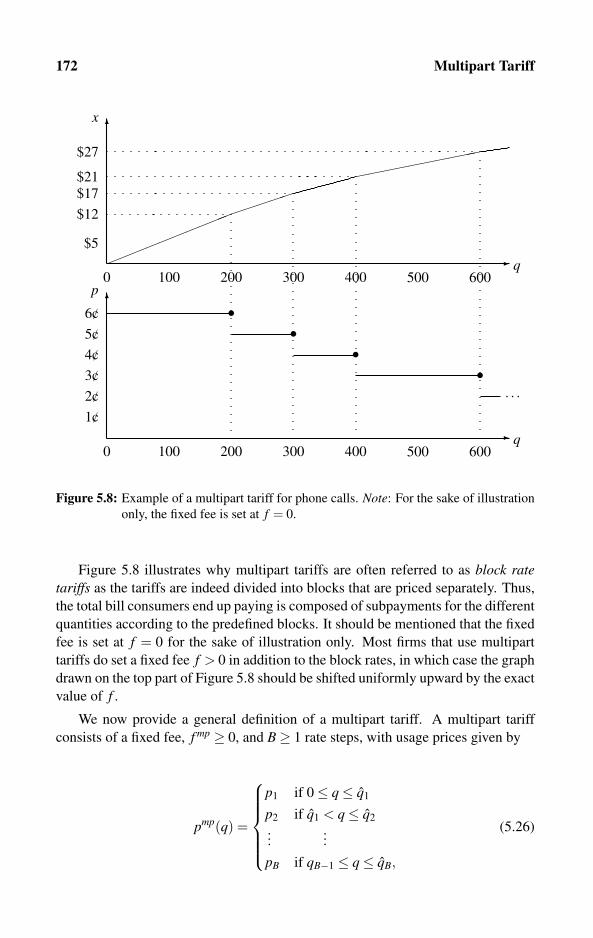
172 Multipart Tariff
0 100 200 300 400 500 600
� q
1/c
2/c
3/c
4/c
5/c
�6/c
0 100 200 300 400 500 600
� q
$5
�
$12
$17$21
$27
••
••
. . .
����
����
��
������
����
p
x
Figure 5.8: Example of a multipart tariff for phone calls. Note: For the sake of illustration
only, the fixed fee is set at f = 0.
Figure 5.8 illustrates why multipart tariffs are often referred to as block ratetariffs as the tariffs are indeed divided into blocks that are priced separately. Thus,
the total bill consumers end up paying is composed of subpayments for the different
quantities according to the predefined blocks. It should be mentioned that the fixed
fee is set at f = 0 for the sake of illustration only. Most firms that use multipart
tariffs do set a fixed fee f > 0 in addition to the block rates, in which case the graph
drawn on the top part of Figure 5.8 should be shifted uniformly upward by the exact
value of f .
We now provide a general definition of a multipart tariff. A multipart tariff
consists of a fixed fee, f mp ≥ 0, and B≥ 1 rate steps, with usage prices given by
pmp(q) =
⎧⎪⎪⎪⎪⎨⎪⎪⎪⎪⎩
p1 if 0≤ q≤ q1
p2 if q1 < q≤ q2
......
pB if qB−1 ≤ q≤ qB,
(5.26)
5.4 Multipart Tariff 173
where 0 < q1 < q2 < · · · < qB ≤ +∞. Clearly, qB < +∞ should be interpreted as
if the seller restricts all consumers to buying no more than qB units (rationing).
In contrast, if qB = +∞, the seller sets B’s usage price for all consumption levels
exceeding qB−1 units. Clearly, if B = 1, the multipart tariff collapses to a two-part
tariff (a fixed fee and a one usage price). As an example, the general formulation
of the six-part tariff (B = 5) described in Table 5.5 can be written as
f mp = 0 and pmp(q) =
⎧⎪⎪⎪⎪⎪⎪⎨⎪⎪⎪⎪⎪⎪⎩
6/c if 0≤ q≤ 200
5/c if 201≤ q≤ 300
4/c if 301≤ q≤ 400
3/c if 401≤ q≤ 600
2/c if q≥ 601.
(5.27)
Clearly, the formulation given in (5.27) assumes that the service/product is indivisi-
ble in the sense that it is sold for whole units only. However, the general formulation
given by (5.26) applies to both cases in which the good is divisible or indivisible.
5.4.2 Multipart versus a menu of two parts: Equivalence results
This section demonstrates that from a technical point of view there is not much
difference between offering consumers a multipart tariff and a menu of multiple
two-part tariffs. Brown and Sibley (1986) attribute the finding of this link to Faul-
haber and Panzar (1977). Here, we demonstrate this link first by constructing a
menu of two-part tariffs that is equivalent to the following multipart tariff defined
by the fixed fee and quantity-dependent marginal usage prices:
f mp = $2 and pmp(q) =
⎧⎪⎨⎪⎩
4/c if 0≤ q≤ 200
2/c if 201≤ q≤ 300
1/c if q≥ 301.
(5.28)
Figure 5.9 depicts the revenue (consumer expenditure) generated by the multi-
part tariff defined by (5.28). Figure 5.9 also demonstrates a geometric methodol-
ogy for how to convert a multipart tariff (with four parts in the present example)
to a menu of multiple two-part tariffs (a menu of three plans in the present case).
Clearly, the two-part tariff corresponding to purchase levels up to q = 200 units
is $2 + 4/cq. Figure 5.9 demonstrates that to find the two-part tariff corresponding
to purchase levels 200 < q ≤ 300, the line corresponding to pB = 2/c needs to be
extended to the left and that the fixed fee fB is determined at the point where the
dashed line intersects the vertical axis, that is, at fB = $6. Similarly, extending the
line corresponding to pC = 1/c leftward determines the third fixed fee, fC = $9. Al-
together, the menu of three two-part tariffs equivalent to the four-part tariff (5.28)
is given by

174 Multipart Tariff
$4
fB = $6
$8
$10
$12
$14 �x
0 100 200 300250
��������������
����
40035015050
������
� q
fC = $9
pA = 4/c
pC = 1/c
pB = 2/c
fA = $2
Figure 5.9: Converting a four-part tariff to a menu of three two-part tariffs.
Plan A: Two-part tariff 〈 fA, pA〉= 〈$2,4/c〉.
Plan B: Two-part tariff 〈 fB, pB〉= 〈$6,2/c〉.
Plan C: Two-part tariff 〈 fC, pC〉= 〈$9,1/c〉.
The geometric method for converting a multipart tariff to a menu of two-part
tariffs illustrated by Figure 5.9 hints that we should also be looking for an algebraic
method for performing the conversion from a multipart tariff to a menu of two-part
tariffs. Obviously, an algebraic method is more convenient, more accurate, and
easy to implement on computers, which would clearly save time. The recursive
algorithm for this conversion is as follows:
Plan A: Set fA = f mp. Hence, fA + pA q = $2+6/cq.
Plan B: Set fB = fA +(pA− pB)qA,B = $2+(4/c−2/c)200 = $6.
Hence, fB + pB q = $6+2/cq.
Plan C: Set fC = fB +(pB− pC)qB,C = $6+(2/c−1/c)300 = $9.
Hence, fC + pC q = $9+1/cq.
Now that the equivalence between a multipart tariff and a menu of two-part tar-
iffs has been established, there is a question as to why multipart tariffs are needed.
Indeed, multipart tariffs are less commonly observed than menus of multiple two-
part tariffs, but multipart tariffs are still used by some service providers. From the
5.4 Multipart Tariff 175
consumers’ point of view, there might be an advantage to accepting a multipart tar-
iff rather than a menu of multiple two-part tariffs if the seller insists that the buyer
commit to one specific tariff plan before the consumer knows the exact consump-
tion level (as happens in most cases). In this case, a multipart tariff offers more
flexibility in the sense that an unexpected rise in consumption will correspond to a
lower rate than a commitment to a specific two-part tariff based on a low expected
consumption level. Of course, the two plans are identical even in this respect if the
seller allows consumers to choose a specific two-part tariff from the menu, even
after the consumer has consumed the service. However, sellers generally insist that
consumers commit to a specific tariff before actual consumption.
One disadvantage that a multipart tariff might have relative to a menu of two-
part tariffs is that it is somewhat harder to compute, and therefore may irritate some
consumers. For example, if a consumer buys q = 350 units and is obligated to pay
according to the multipart tariff illustrated in Figure 5.9, the bill should include the
rather complicated computation given by
$2+4/c ·200+2/c ·100+1/c ·50 = $12.5.
This is somewhat more complicated than computing the equivalent menu of two-
part tariffs given by
Plan A : $2+6/c ·350 = $23.
Plan B : $6+4/c ·350 = $20.
Plan C : $9+1/c ·350 = $12.5.
We conclude this section with the general formulation of the menu of B two-
part tariffs, which is equivalent to the (B + 1)-part tariff defined by (5.26). Thus,
the recursive sequence of fixed fees is given by
f1 = f mp.
f2 = f1 +(p1− p2)q1.
......
... (5.29)
fi = fi−1 +(pi−1− pi)qi−1.
......
...
fB = fB−1 +(pB−1− pB)qB−1.
The general formulation given in (5.29) relies on the assumption that the usage
prices listed in (5.26) satisfy p1 > p2 > · · ·> pB, which means that larger quantities
are discounted in terms of the usage price. The algorithm described by (5.29) may
not work if some of these inequality signs are reversed.
Finally, it should be noted that the established equivalence between multipart
tariffs and a menu of two-part tariffs also holds with respect to implementation
176 Multipart Tariff
difficulties stemming from the incentive compatibility constraints that we have al-
ready discussed in Section 5.3. That is, very often it is hard to find multipart tariffs
that would segment the market among consumers so that consumers of different
types end up paying different usage rates according to (5.26).
5.5 Regulated Public Utility
Our analysis of multipart tariffs focuses on profit-maximizing firms. However, most
of the academic research on multipart tariffs in general and two-part tariffs in par-
ticular is confined to regulated firms such as electricity, phone, and gas companies.
These types of firms are called public utilities. Until very recently, these public util-
ities were not allowed to set their own tariffs. Instead, states established regulatory
commissions that determined the exact rates that consumers were charged. Read-
ers who wish to learn more about the wide variety of regulated tariffs commonly
practiced by public utilities can consult some classic books by Brown and Sibley
(1986), Crew and Kleindorfer (1986), and Wilson (1993).
There are two (related) major differences between a monopoly firm and a reg-
ulated public utility with respect to the setting of two-part tariffs.
(a) A monopoly firm attempts to extract maximum surplus from consumers. In
contrast, the regulator seeks to maximize social welfare, which, for the case of
a single firm, is commonly defined as
W (q1, . . . ,qM) def=M
∑�=1
gcs�(q�)+π
(M
∑�=1
q�
). (5.30)
Thus, for most purposes, social welfare is defined as the sum of consumers’
gross surpluses and the profit made by the regulated firm (which is a function
of total output sold to consumers).
(b) The regulator must ensure that total consumer spending covers not only vari-
able costs but also the fixed cost φ borne by these public utilities. In contrast,
the objective of an unregulated monopoly is to extract maximum surplus from
consumers.
(c) A regulator may consider giving a subsidy (or a tax break) to a public utility.
However, our analysis here is confined to a firm that always breaks even, so a
subsidy is not needed.
Note that utility suppliers often bear extremely high fixed costs that may involve
repaying for their investments in infrastructure. These investments are essential
for the purpose of transmitting these utilities directly to consumers’ homes. In

5.5 Regulated Public Utility 177
addition, fixed costs never cease, even after all loans are repaid, because of the
need for continuous maintenance of these infrastructures.
As it turns out, both a regulator who seeks economic efficiency and a single
seller seeking to maximize profit only find the two-part tariff extremely useful be-
cause the fixed part f 2p can be set so that consumers pay their share in the large
fixed costs borne by firms, φ , whereas the per-unit usage fee p2p can be set to cover
the variable cost associated with the marginal cost μ . In fact, if all consumers are
of the same type, both the regulator and the single seller can set the two-part tariff
at certain levels that maximize social welfare. The only difference is the amount of
surplus extracted from consumers. Whereas the regulator seeks to use the fixed fee
to pay for firms’ fixed costs only, a monopoly firm attempts to extract maximum
surplus from consumers.
If all N consumers are of the same type (sharing identical demand functions)
the socially optimal two-part tariff, that is, a tariff that maximizes (5.30), is
f 2p =φN
and p2p = μ. (5.31)
Under this tariff, each consumer pays an equal share of the fixed cost φ . The
resulting consumption levels are identical to levels consumed under a two-part tariff
set by a profit-maximizing firm given by (5.8).
Suppose now that there are M types of consumers, each having a different de-
mand function. A natural extension of the two-part tariff designed for a single con-
sumer type (5.31) to multiple consumer types would be to set the socially optimal
two-part tariff to
f 2p =φ
∑M�=1 N�
and p2p = μ. (5.32)
Here, the fixed cost is also equally divided among all the consumers, hence the firm
also breaks even.
Our analysis could end here if the tariff (5.32) would be a feasible solution to all
possible configurations of consumer types. However, as it turns out, the proposed
socially optimal two-part tariff (5.32) is not feasible if some consumers have low
demand in the sense that their derived gross consumer surplus is lower than the sum
of their expenditure. Formally, if under this tariff, a type � consumer realizes that
gcs�(q2p� ) < f 2p + p2pq2p
� , the consumer will not buy this service.
To demonstrate this case, suppose now that there are N1 = 600 type 1 consumers
and N2 = 400 type 2 consumers. Further, suppose that the demand functions of the
two types are given by (5.12), which are also plotted in Figure 5.4. Finally, assume
that the firm’s marginal cost is μ = $2 and that the firm bears a fixed cost of $5000.
Because there are N1 + N2 = 600 + 400 = 1000 consumers, the candidate socially
optimal two-part tariff should take the form of
f 2p =φ
∑M�=1 N�
=$5000
600+400= $5 and p2p = $2. (5.33)

178 Multipart Tariff
However, inspection of Table 5.2 reveals that no type 2 consumer would be willing
to pay a fixed fee exceeding $4 when the usage price is set at p2p = $2. Hence,
type 2 consumers will not buy this service. Furthermore, because under the tariff
(5.33) only the N1 = 600 consumers buy, the firm is making a loss given by π =600[$5+($2−$2)3]−$5000 =−$2000 < 0. To break even, the regulator will be
forced to raise the fixed fee to f 2p = φ/N1 = 5000/600 = $8.34. A type 1 consumer
will still buy at this fee because Table 5.2 shows that type 1 consumers will buy as
long as p2p = $2 and f 2p < $9.
Now, will the setting of the fixed fee to equal f 2p = $8.34 solve the regulator’s
problem? The answer depends on the goal of the regulator. If the regulator cannot
price discriminate between the two consumer types and is restricted to setting one
two-part tariff for all consumers, and if the objective of the regulator is to maximize
the social welfare function (5.30), then f 2p = $8.34 may be a solution. However,
unlike unregulated monopoly firms, regulators are often very sensitive to the ex-
clusion of consumers from various groups of society. For example, in the case of
basic phone services, if type 2 consumers happen to be low-income families, regu-
lators may decide to deviate from the objective function (5.30) and even decide to
subsidize part of the fixed cost using taxpayers’ money.
Finally, if the regulator is able to price discriminate between the consumer
types, say on the basis of age, income, or profession, the regulator can simply
set different two-part tariffs for different consumer groups. A good design of such
a scheme could result in an even higher welfare level compared with the adoption
of Ramsey pricing analyzed in Section 3.6.2.
5.6 Exercises
1. In the market in which your firm is selling, the demand function by each in-
dividual is approximated by a linear function given by p = 120− 0.5q. The
marginal production cost is μ = $40, and the fixed cost is denoted by φ . Solve
the following problems.
(a) Similar to Figure 5.2, draw the demand curve and compute the two-part
tariff f 2p and p2p that maximizes your firm’s profit.
(b) Suppose now that there are N = 5 consumers with the same demand func-
tion. Compute the profit level assuming that the fixed cost is φ = $30,000.
2. As the new VP for pricing of BLABLA, a cell-phone operator, you are in charge
of proposing a two-part tariff structure for your customers. Your research depart-
ment has just completed a market survey concluding that there is only one con-
sumer (N = 1), whose demand data are summarized in Table 5.6. The marginal
cost of a unit of phone calls is μ = 10/c and the fixed cost is φ = 20/c. Using
the analysis in Section 5.1.3, fill in the missing items in the middle section of
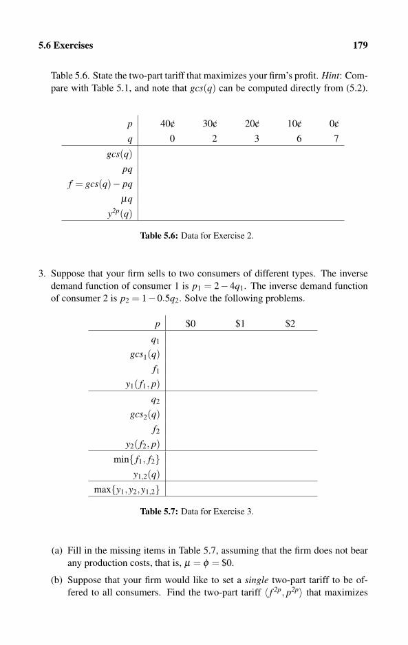
5.6 Exercises 179
Table 5.6. State the two-part tariff that maximizes your firm’s profit. Hint: Com-
pare with Table 5.1, and note that gcs(q) can be computed directly from (5.2).
p 40/c 30/c 20/c 10/c 0/c
q 0 2 3 6 7
gcs(q)pq
f = gcs(q)− pq
μq
y2p(q)
Table 5.6: Data for Exercise 2.
3. Suppose that your firm sells to two consumers of different types. The inverse
demand function of consumer 1 is p1 = 2− 4q1. The inverse demand function
of consumer 2 is p2 = 1−0.5q2. Solve the following problems.
p $0 $1 $2
q1
gcs1(q)f1
y1( f1, p)
q2
gcs2(q)f2
y2( f2, p)
min{ f1, f2}y1,2(q)
max{y1,y2,y1,2}
Table 5.7: Data for Exercise 3.
(a) Fill in the missing items in Table 5.7, assuming that the firm does not bear
any production costs, that is, μ = φ = $0.
(b) Suppose that your firm would like to set a single two-part tariff to be of-
fered to all consumers. Find the two-part tariff 〈 f 2p, p2p〉 that maximizes
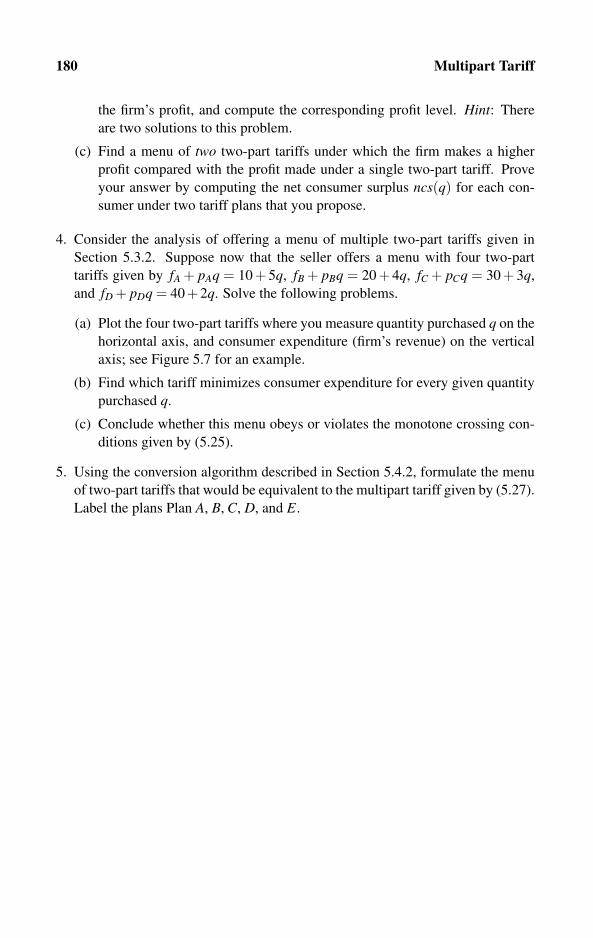
180 Multipart Tariff
the firm’s profit, and compute the corresponding profit level. Hint: There
are two solutions to this problem.
(c) Find a menu of two two-part tariffs under which the firm makes a higher
profit compared with the profit made under a single two-part tariff. Prove
your answer by computing the net consumer surplus ncs(q) for each con-
sumer under two tariff plans that you propose.
4. Consider the analysis of offering a menu of multiple two-part tariffs given in
Section 5.3.2. Suppose now that the seller offers a menu with four two-part
tariffs given by fA + pAq = 10 + 5q, fB + pBq = 20 + 4q, fC + pCq = 30 + 3q,
and fD + pDq = 40+2q. Solve the following problems.
(a) Plot the four two-part tariffs where you measure quantity purchased q on the
horizontal axis, and consumer expenditure (firm’s revenue) on the vertical
axis; see Figure 5.7 for an example.
(b) Find which tariff minimizes consumer expenditure for every given quantity
purchased q.
(c) Conclude whether this menu obeys or violates the monotone crossing con-
ditions given by (5.25).
5. Using the conversion algorithm described in Section 5.4.2, formulate the menu
of two-part tariffs that would be equivalent to the multipart tariff given by (5.27).
Label the plans Plan A, B, C, D, and E.

Chapter 6
Peak-load Pricing
6.1 Seasons, Cycles, and Service-cost Definitions 183
6.1.1 Seasons and cycles
6.1.2 Three types of costs
6.2 Two Seasons: Fixed-peak Case 185
6.2.1 Winters and summers: An example
6.2.2 Two seasons: General formulation for the fixed-peak case
6.3 Two Seasons: Shifting-peak Case 190
6.3.1 Winters and summers: An example
6.3.2 Two seasons: General formulation for shifting peak
6.4 General Computer Algorithm for Two Seasons 194
6.5 Multi-season Pricing 194
6.5.1 Multi-season pricing: A three-season example
6.5.2 Multi-season pricing: Method and computer algorithm
6.6 Season-interdependent Demand Functions 201
6.6.1 Winters and summers: An example
6.6.2 Interdependent demand: General formulation
6.7 Regulated Public Utility 205
6.7.1 Winters and summers: An example
6.7.2 Two seasons: General formulation and computer algorithm
6.7.3 Multi-season pricing: A three-season example
6.7.4 Multi-season pricing: General formulation for public utility
6.8 Demand, Cost, and the Lengths of Seasons 214
6.8.1 Daytime and nighttime supply of electricity: Examples
6.8.2 General formulations
6.9 Exercises 223

182 Peak-load Pricing
Services constitute what economists call nonstorable goods. Electricity, telephone,
transportation, banking, and most other services are consumed at the time of pur-
chase. This nonstorability characteristic of services may lead to congestion of ser-
vice systems when the demand for the service is unevenly distributed among dif-
ferent periods or seasons. The demand for telephone services is at the highest level
during daytime, during weekdays, and tends to be lower during nights, weekends,
and some holidays. The demand for air travel for most places tends to be relatively
high during the summer, whereas the demand for transportation to ski resorts is
greatly enhanced during the winter. Electricity use follows a daily cycle related
partly to the use of appliances and lighting devices. In addition, it also follows a
yearly cycle because of climatic changes. Thus, the demand follows several, some-
times overlapping, periodic cycles.
Peak-load pricing techniques are commonly observed in vacation-related ser-
vices (airline, restaurant, and hotel industries) as well as in utility services (phone
and electricity). The utilization of peak-load pricing techniques is profitable in
industries with the following main characteristics:
(a) Demand varies significantly among the different seasons.
(b) Services are time-related and perishable in the sense that they cannot be post-
poned or delivered earlier than the scheduled time of delivery.
(c) Service providers must acquire a significant amount of costly capital.
(d) The acquired capital cannot be easily liquidated and cannot be easily rented out
or sold to other firms.
Clearly, the airline industry possesses all of the above-listed characteristics, because
traveling in the winter differs from traveling during the summer. In addition, air-
lines must invest in acquiring expensive aircraft and must precontract gates, parking
spots, and other services at various airports. Finally, aircraft cannot be easily liq-
uidated at the price purchased, even if depreciation is deducted from the price of
new aircraft. Electricity and phone companies also exhibit the same characteristics
because they must also invest in illiquid and costly equipment. In addition, the
demand for electricity and phone calls fluctuates according to the hours of the day,
and days of the week, and across the different seasons in a given year.
To summarize, the nonstorability of services together with periodic fluctuations
in demand makes the peak-load pricing mechanism both profitable and socially
efficient. If instead prices were uniform across seasons, the quantity demanded
would rise and fall as the seasons changed. To meet demand at peak seasons would
then require the installation of capacity, which would be underused during off-peak
seasons. Because capacity can be highly costly to buy and maintain, the resulting
idleness during off-peak seasons would be highly inefficient. On this basis, peak-

6.1 Seasons, Cycles, and Service-cost Definitions 183
load pricing can partially fix this inefficiency by lowering the price during off-peak
seasons, thereby reducing the amount of idle capacity.
In solving the peak-load pricing problem, the seller has to make the following
two major decisions:
(a) How much capital to invest in, and hence how much production capacity to
maintain to be able to meet demand in the peak season.
(b) How to price this service in each season.
There is a vast literature on peak-load pricing, which is surveyed in Crew,
Fernando, and Kleindorfer (1995), and in some classic books such as Crew and
Kleindorfer (1979, 1986), Brown and Sibley (1986), and Sherman (1989). Boiteux
(1960), Steiner (1957), Hirshleifer (1958), and Williamson (1966) are considered
to be highly influential papers on peak-load pricing. The survey and the above-
mentioned books also discuss additional topics that are not addressed in this book,
such as multiple technologies and issues related to uncertainty that may lead to
rationing and outage costs.
6.1 Seasons, Cycles, and Service-cost Definitions
To maintain service capacity, the provider must invest in building some capital
stock. Investment in service capacity allows the firm to provide service over time.
The way costs are defined plays a crucial role in successful and profitable imple-
mentation of peak-load pricing strategies. Readers are urged to consult Section 6.8,
which analyzes various possible cost accounting methods, taking into account the
relative duration of each season over a cycle.
6.1.1 Seasons and cycles
We use the general term season to represent a certain time interval during which
the demand is kept more or less stable. Seasons could be daytime, nighttime, week-
days, weekends, and of course, summer and winter.
Seasons will be indexed by t = A,B, . . . ,T or by t = 1,2, . . . ,T . Let pt denote
the price in season t and qt denote quantity of service demanded and supplied in
each season t. Before we formally begin to write down the firm’s cost function, we
must further extend our discussion of cycles of seasons. We define a cycle as the
time interval consisting of one full cycle of all seasons. For example, a cycle called
one year consists of four seasons called summer, fall, winter, and spring. Alterna-
tively, if we wish to simplify our pricing strategy, we can divide a cycle of one year
into summer and winter only. Table 6.1 provides some additional examples.
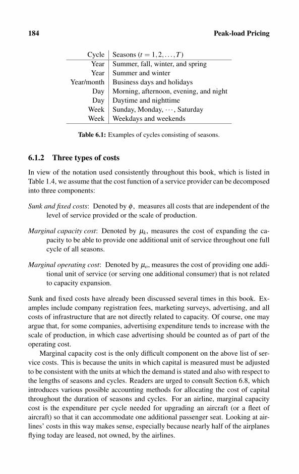
184 Peak-load Pricing
Cycle Seasons (t = 1,2, . . . ,T )
Year Summer, fall, winter, and spring
Year Summer and winter
Year/month Business days and holidays
Day Morning, afternoon, evening, and night
Day Daytime and nighttime
Week Sunday, Monday, · · · , Saturday
Week Weekdays and weekends
Table 6.1: Examples of cycles consisting of seasons.
6.1.2 Three types of costs
In view of the notation used consistently throughout this book, which is listed in
Table 1.4, we assume that the cost function of a service provider can be decomposed
into three components:
Sunk and fixed costs: Denoted by φ , measures all costs that are independent of the
level of service provided or the scale of production.
Marginal capacity cost: Denoted by μk, measures the cost of expanding the ca-
pacity to be able to provide one additional unit of service throughout one full
cycle of all seasons.
Marginal operating cost: Denoted by μo, measures the cost of providing one addi-
tional unit of service (or serving one additional consumer) that is not related
to capacity expansion.
Sunk and fixed costs have already been discussed several times in this book. Ex-
amples include company registration fees, marketing surveys, advertising, and all
costs of infrastructure that are not directly related to capacity. Of course, one may
argue that, for some companies, advertising expenditure tends to increase with the
scale of production, in which case advertising should be counted as of part of the
operating cost.
Marginal capacity cost is the only difficult component on the above list of ser-
vice costs. This is because the units in which capital is measured must be adjusted
to be consistent with the units at which the demand is stated and also with respect to
the lengths of seasons and cycles. Readers are urged to consult Section 6.8, which
introduces various possible accounting methods for allocating the cost of capital
throughout the duration of seasons and cycles. For an airline, marginal capacity
cost is the expenditure per cycle needed for upgrading an aircraft (or a fleet of
aircraft) so that it can accommodate one additional passenger seat. Looking at air-
lines’ costs in this way makes sense, especially because nearly half of the airplanes
flying today are leased, not owned, by the airlines.
6.2 Two Seasons: Fixed-peak Case 185
For an electricity company, marginal capacity cost is the expenditure per one
cycle of upgrading a generator so it can generate one additional kilowatt of electric-
ity. For a phone operator, marginal capacity cost may include the cost of enhancing
the network to be able to accommodate one additional phone call, or an additional
phone line.
Marginal operating cost of an airline includes the cost of in-flight services
needed for accommodating one additional passenger, such as food, boarding per-
sonnel, and entertainment. Marginal operating cost of an electrical power company
consists of the additional expenditure on coal, gas, fuel, oil, and labor attributed
to increasing electricity output by an additional kilowatt-hour. Marginal operating
cost of a telephone company is negligible. However, some economists may count
the cost of congestion as part of the operating cost because when the system op-
erates near full capacity, customers are likely to receive busy signals. Congestion
cost is most noticeable on the Internet, when the response time could become very
long when the network operates near full capacity.
It should be emphasized that the two types of marginal costs defined above dif-
fer substantially with respect to their time span (see Section 6.8 for a discussion of
problems related to capital cost accounting). More precisely, the marginal capacity
cost is configured on a cost basis adjusted for exactly one full cycle of all seasons.
Thus, if we associate a cycle with one year, an airline that buys aircraft lasting for
10 years should divide the total cost spent on this capital by 10 years and then by
the total (daily) capacity of the acquired fleet. An easier way of looking at this is to
assume that the purchase of capital is fully financed by commercial banks. Under
this interpretation, the yearly cost equals the interest payments made to the bank
for this loan, divided by the service capacity of this capital (number of passengers
that can be flown on these aircraft). Deprecation cost of capital can also be added.
In contrast, the marginal operating cost is the cost per served customer, so it does
not bear any time dimension. Table 6.2 provides some further examples. Table 6.2
demonstrates the difference between marginal capacity cost μk and marginal op-
erating cost μo. The marginal operating cost is materialized only when and if a
customer is actually being served. In contrast, the marginal capacity cost is based
on potential service capacity. In this aspect, this distinction very much resembles
the distinction made in Definition 8.4 in the context of refunds on no-shows. Us-
ing the airline example, total operating cost is computed by multiplying μo by the
actual demand level in a particular season. In contrast, total capacity cost is chosen
at the procurement stage and cannot vary or fluctuate with the demand across the
seasons in a given cycle.
6.2 Two Seasons: Fixed-peak Case
The fixed-peak season analysis applies to markets where the demand level varies
significantly between the seasons. The exact measure to determine whether there
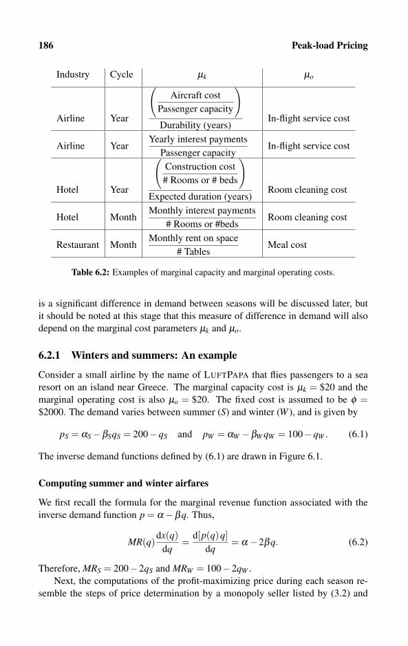
186 Peak-load Pricing
Industry Cycle μk μo
Airline Year
(Aircraft cost
Passenger capacity
)
Durability (years)In-flight service cost
Airline YearYearly interest payments
Passenger capacityIn-flight service cost
Hotel Year
(Construction cost
# Rooms or # beds
)
Expected duration (years)Room cleaning cost
Hotel MonthMonthly interest payments
# Rooms or #bedsRoom cleaning cost
Restaurant MonthMonthly rent on space
# TablesMeal cost
Table 6.2: Examples of marginal capacity and marginal operating costs.
is a significant difference in demand between seasons will be discussed later, but
it should be noted at this stage that this measure of difference in demand will also
depend on the marginal cost parameters μk and μo.
6.2.1 Winters and summers: An example
Consider a small airline by the name of LUFTPAPA that flies passengers to a sea
resort on an island near Greece. The marginal capacity cost is μk = $20 and the
marginal operating cost is also μo = $20. The fixed cost is assumed to be φ =$2000. The demand varies between summer (S) and winter (W ), and is given by
pS = αS−βSqS = 200−qS and pW = αW −βW qW = 100−qW . (6.1)
The inverse demand functions defined by (6.1) are drawn in Figure 6.1.
Computing summer and winter airfares
We first recall the formula for the marginal revenue function associated with the
inverse demand function p = α−βq. Thus,
MR(q)dx(q)
dq=
d[p(q)q]dq
= α−2βq. (6.2)
Therefore, MRS = 200−2qS and MRW = 100−2qW .
Next, the computations of the profit-maximizing price during each season re-
semble the steps of price determination by a monopoly seller listed by (3.2) and
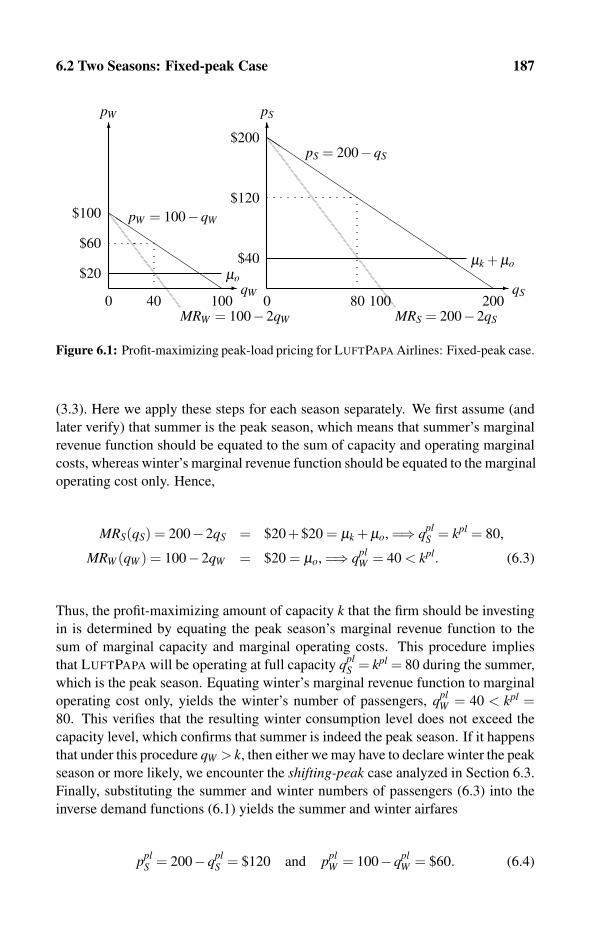
6.2 Two Seasons: Fixed-peak Case 187
�
�
������������������
0
pS
qS
$200
200
$40
100MRS = 200−2qS
80
$120
μk + μo
�
�
���
��
��
��
0
pW
$100
100
$20 μo
MRW = 100−2qW
40
$60
qW
pS = 200−qS
pW = 100−qW
Figure 6.1: Profit-maximizing peak-load pricing for LUFTPAPA Airlines: Fixed-peak case.
(3.3). Here we apply these steps for each season separately. We first assume (and
later verify) that summer is the peak season, which means that summer’s marginal
revenue function should be equated to the sum of capacity and operating marginal
costs, whereas winter’s marginal revenue function should be equated to the marginal
operating cost only. Hence,
MRS(qS) = 200−2qS = $20+$20 = μk + μo, =⇒ qplS = kpl = 80,
MRW (qW ) = 100−2qW = $20 = μo, =⇒ qplW = 40 < kpl. (6.3)
Thus, the profit-maximizing amount of capacity k that the firm should be investing
in is determined by equating the peak season’s marginal revenue function to the
sum of marginal capacity and marginal operating costs. This procedure implies
that LUFTPAPA will be operating at full capacity qplS = kpl = 80 during the summer,
which is the peak season. Equating winter’s marginal revenue function to marginal
operating cost only, yields the winter’s number of passengers, qplW = 40 < kpl =
80. This verifies that the resulting winter consumption level does not exceed the
capacity level, which confirms that summer is indeed the peak season. If it happens
that under this procedure qW > k, then either we may have to declare winter the peak
season or more likely, we encounter the shifting-peak case analyzed in Section 6.3.
Finally, substituting the summer and winter numbers of passengers (6.3) into the
inverse demand functions (6.1) yields the summer and winter airfares
pplS = 200−qpl
S = $120 and pplW = 100−qpl
W = $60. (6.4)
188 Peak-load Pricing
The resulting total profit earned by LUFTPAPA in one cycle (consisting of one sum-
mer and one winter season) is
ypl = (pplW −μo)q
plW +(ppl
S −μk−μo)qplS −φ
= (60−20)40+(120−20−20)80−2000 = $6000. (6.5)
The logic behind the method demonstrated above, which is also illustrated in
Figure 6.1, is that the seller invests in the last unit of capacity to be able to accom-
modate the extra seating capacity needed to satisfy the peak-season demand (which
happens to be the summer season in the present example). Therefore, the cost of
capacity should be attributed to summer passengers only because the winter pas-
sengers are served on an underused capacity, and adding an additional passenger
during the winter does not require any extra investment in capacity.
Why is peak-load pricing profitable?
The reader may ask why peak-load pricing is more profitable than charging a uni-
form price across all seasons. To answer this question, we need to recall our analy-
sis of discriminating monopoly selling in two markets with different demand curves
(see Section 3.2.4). In view of Figure 6.1, LUFTPAPA Airlines can choose between
two uniform prices. It can charge a low price p < $100, thereby serving both sum-
mer and winter passengers. Alternatively, it can charge a high price p ≥ $100,
thereby excluding all winter passengers, thereby resorting to summer operation
only.
For any uniform price in the range 0 < pS,W < $100, the aggregate direct de-
mand function is qS,W = 200− p + 100− p = 300− 2pS,W . Therefore, the ag-
gregate inverse demand function is pS,W = 150− qS,W /2. By the formula given
in (6.2), the aggregate marginal revenue function is MRS,W (qS,W ) = 150− qS,W .
Setting MRS,W (qS,W ) = μk + μo = $40 yields qS,W = 110 and therefore a price
pS,W = 150− qS,W /2 = $95 < $100. Hence, both markets are indeed served at
this price.
Before we compute the total profit generated by setting pS,W = $95 and serv-
ing both markets, we must figure out how much aircraft seating capacity LUFT-
PAPA should invest to be able to meet this demand. Because qS = 200−95 = 105,
whereas qW = 100−95 = 5, to be able to accommodate all passengers in each sea-
son, LUFTPAPA Airlines must invest in a seating capacity of 105. Therefore, the
profit of LUFTPAPA from serving summer and winter passengers under uniform
prices across both seasons is
yS,W = (pS,W −μo)qS,W −μkqS−φ =
(95−20)110−20 ·105−2000 = $4,150 < $6,000 = ypl, (6.6)
which is lower than the profit generated under peak-load pricing.

6.2 Two Seasons: Fixed-peak Case 189
Next, under uniform pricing, the seller also computes the profit when the seller
raises the price above $100, in which case, in view of Figure 6.1, only summer
passengers will book their flights with the airline. However, the top line in equation
(6.3) already provides the solution qS = 80 passengers. The corresponding price
pS = $120 was already computed in (6.4). In this case, the profit is given by
yS = (pS−μk−μo)qS−φ
= (120−20−20)80−2000 = $4400 < $6000 = ypl. (6.7)
This concludes the proof showing why peak-load pricing is more profitable than
uniform pricing. Clearly, this formal proof was not really needed because one can
simply adopt a revealed preference argument to prove it. More precisely, under
peak-load pricing, the seller can always choose to set pS = pW . However, if the
firm chooses (as our computations above recommend) to set unequal prices across
the seasons so that pS �= pW , then it must be enhancing its profit. However, from
time to time, such a comparison may be needed if the cost of implementing peak-
load pricing is significantly higher than the cost of marketing under a single uniform
price.
6.2.2 Two seasons: General formulation for the fixed-peak case
This section extends the two-season airline example of the previous section to gen-
eral linear demand functions pA = αA−βAqA during season A, and pB = αB−βBqB
during season B. The single seller’s fixed cost is φ , marginal capacity cost is μk,
and marginal operating cost is μo (see Section 6.1 for precise definitions). It must
be verified first that either αA > μk + μo or αB > μk + μo, which is a necessary
(but not sufficient) condition for making nonnegative profit. In addition, it must be
verified that consumers’ willingness to pay exceeds the marginal operating cost so
that αA > μo and αB > μo.
The computation of the profit-maximizing price in each season should follow
the following steps:
Step I: Check if A is the peak season by setting MRA(qA) = αA−2βAqA = μk + μo
to obtain
qA =αA−μk−μo
2βAand pA =
αA + μk + μo
2. (6.8)
Similarly, for season B (off-peak season) set MRB(qB) = αB−2βBqB = μo to
obtain
qB =αB−μo
2βBand pB =
αB + μo
2. (6.9)
Now, check if A is indeed the peak season so that qB ≤ qA. If this is the case,
then set the capacity level to k = qA and skip to Step III.

190 Peak-load Pricing
Step II: Check if B is the peak season by setting MRB(qB) = αB−2βBqB = μk +μo
to obtain
qB =αB−μk−μo
2βBand pB =
αB + μk + μo
2. (6.10)
Similarly, for season A (off-peak season) set MRA(qA) = αA−2βAqA = μo to
obtain
qA =αA−μo
2βAand pA =
αA + μo
2. (6.11)
Now, check if B is indeed the peak season so that qA ≤ qB. If this is the case,
then set the capacity level to k = qB. If this is not the case, stop here as you
reached the shifting-peak case analyzed in Section 6.3.
Step III: Compute the profit level using the relevant prices and quantities computed
in Step I or Step II above. Thus,
ypl =
{(ppl
A −μk−μo)qplA +(pB−μo)q
plB −φ if A is the peak
(pplA −μk)q
plA +(ppl
B −μk−μo)qplB −φ if B is the peak.
(6.12)
Then, verify that the firm does not make a loss by checking whether ypl ≥ 0.
The above algorithm indicates that the marginal cost of capacity (capital)
should be attributed to the peak-season consumers only. In particular, the
profit function (6.12) indicates that the cost of capital μk maxqA,qB should
be counted only once, because capital is assumed to be durable for the entire
cycle consisting of season A and season B.
6.3 Two Seasons: Shifting-peak Case
The case of shifting peak has been analyzed in Steiner (1957). Bailey and White
(1974) pointed out the possibility of peak reversals. Shifting peak occurs when
the marginal capacity cost μk is relatively high so that it cannot be charged to the
peak-season consumers only. In this case, capacity cost should be shared among
consumers in all seasons. Another way of looking at this is to realize that a rise in
the price of capital raises the cost of maintaining idle capacity during the low sea-
son. Hence, for a sufficiently high cost of capital, the seller should adjust seasonal
prices so that capacity is fully used in all seasons, in which case the seller sells
equal amounts in all seasons. Shifting peak is also likely to occur when there are
only small variations in demand across the different seasons. In either case, the al-
gorithm described in Section 6.2 for the fixed-peak case cannot be used. Therefore,
the algorithm developed in this section is based on the principle that consumers in
all seasons should be charged for the use of capacity, and the key question is how
to split this cost of capital among consumers from different seasons. As before, we
also need to compute the profit-maximizing amount of investment in capacity.
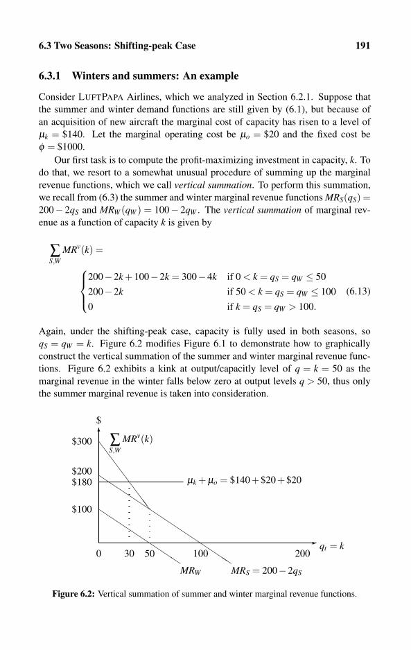
6.3 Two Seasons: Shifting-peak Case 191
6.3.1 Winters and summers: An example
Consider LUFTPAPA Airlines, which we analyzed in Section 6.2.1. Suppose that
the summer and winter demand functions are still given by (6.1), but because of
an acquisition of new aircraft the marginal cost of capacity has risen to a level of
μk = $140. Let the marginal operating cost be μo = $20 and the fixed cost be
φ = $1000.
Our first task is to compute the profit-maximizing investment in capacity, k. To
do that, we resort to a somewhat unusual procedure of summing up the marginal
revenue functions, which we call vertical summation. To perform this summation,
we recall from (6.3) the summer and winter marginal revenue functions MRS(qS) =200− 2qS and MRW (qW ) = 100− 2qW . The vertical summation of marginal rev-
enue as a function of capacity k is given by
∑S,W
MRv(k) =
⎧⎪⎨⎪⎩
200−2k +100−2k = 300−4k if 0 < k = qS = qW ≤ 50
200−2k if 50 < k = qS = qW ≤ 100
0 if k = qS = qW > 100.
(6.13)
Again, under the shifting-peak case, capacity is fully used in both seasons, so
qS = qW = k. Figure 6.2 modifies Figure 6.1 to demonstrate how to graphically
construct the vertical summation of the summer and winter marginal revenue func-
tions. Figure 6.2 exhibits a kink at output/capacitly level of q = k = 50 as the
marginal revenue in the winter falls below zero at output levels q > 50, thus only
the summer marginal revenue is taken into consideration.
�
0qt = k
20010050
�
���������
���������������
MRW
��������
MRS = 200−2qS
$
$300
$200
$100
30
$180 μk + μo = $140+$20+$20
∑S,W
MRv(k)
Figure 6.2: Vertical summation of summer and winter marginal revenue functions.
192 Peak-load Pricing
The vertical sum ∑MRv(k) has the following interpretation: It reflects the ad-
ditional revenue that can be generated by expanding capacity by one additional
seat. Because under the shifting peak case prices are set so that passenger demand
reaches full capacity in both seasons, the sum of the two marginal revenue functions
reflects the revenue gain from investing in an additional passenger seat. The reader
should be aware of the difference between vertical and horizontal summations of
marginal revenue and demand functions. For a comparison between vertical and
horizontal summations, the reader can refer to Section 2.5, which focuses on hori-
zontal summations.
Figure 6.2 illustrates that the profit-maximizing capacity level is determined
by equating the vertical sum of the marginal revenue functions with the sum of
marginal capacity and operating costs. Formally, solving
∑S,W
MRv(k) = 300−4k = $140+$20+$20 = $180 = μk +2μo (6.14)
yields
kpl = qplS = qpl
W = 30, pplS = 200−30 = $170,
and pplW = 100−30 = $70. (6.15)
Notice that the marginal capacity cost μk appears only once, whereas the marginal
operating cost appears twice in the profit-maximization condition (6.14). This fol-
lows from our assumptions that capital is durable and that the cost of capacity is
computed on the basis of an entire cycle (one year in the present example). In
contrast, the marginal operating cost applies only for passengers who are actually
being served and therefore must be added up across all seasons (winter and summer
in the present example). Finally, total profit is given by
ypl = (170−20)30+(70−20)30−140 ·30−1000 = $800. (6.16)
6.3.2 Two seasons: General formulation for shifting peak
This section extends the two-season airline example of Section 6.3.1 to general
linear demand functions pA = αA− βAqA and pB = αB− βBqB. The seller bears
a fixed cost of φ , marginal capacity cost μk, and marginal operating cost μo (see
Section 6.1 for precise definitions). It must be verified first that either αA > μk +μo
or αB > μk + μo, which is a necessary (but not sufficient) condition for making
nonnegative profit. In addition, it must be verfied that consumers’ willingness to
pay also exceeds the marginal operating cost, so αA > μo and αB > μo.
The computation of the profit-maximizing price in each season follows the fol-
lowing steps:
6.3 Two Seasons: Shifting-peak Case 193
Step I: Verify that A is not a peak season by setting MRA(qA) = αA− 2βAqA =μk +2μo to obtain
qA =αA−μk−μo
2βAand pA =
αA + μk + μo
2. (6.17)
Similarly, for season B, set MRB(qB) = αB−2βBqB = μo to obtain
qB =αB−μo
2βBand pB =
αB + μo
2. (6.18)
Now, verify that A is not a peak season by confirming that qB > qA. If this
is not the case, stop here as you have reached the fixed-peak case that was
analyzed in Section 6.2.
Step II: Verify that B is not a peak season by setting MRB(qB) = αB− 2βBqB =μk + μo to obtain
qB =αB−μk−μo
2βBand pB =
αB + μk + μo
2. (6.19)
Similarly, for season A, set MRA(qA) = αA−2βAqA = μo to obtain
qA =αA−μo
2βAand pA =
αA + μo
2. (6.20)
Now, confirm that B is not a peak season by verifying that qA > qB. If this
is not the case, stop here as you have reached the fixed-peak case that was
already analyzed in Section 6.2.
Step III: Sum up vertically the two marginal revenue functions and equate the sum
to the sum of marginal capacity and marginal operating costs over a full cycle
∑A,B
MRv(k) = αA +αB−2(βA +βB)k = μk +2μo, (6.21)
which obtains the desired capacity level
kpl = qplA = qpl
B =αA +αB−μk−2μo
2(βA +βB). (6.22)
Step IV: Substitute kpl = qplA = qpl
B into each demand function to obtain the price in
each season:
pplA =
αA(βA +2βB)+βA(μk +2μo−αB)2(βA +βB)
, (6.23)
pplB =
αB(2βA +βB)+βB(μk +2μo−αA)2(βA +βB)
.
194 Peak-load Pricing
Observe that unlike the prices set under the fixed-peak case given by (6.8)–(6.11),
here the marginal capacity cost μk directly affects the prices in both seasons, not
only the summer price. This is a direct consequence of the outcome that capacity
is fully used in all both seasons. The resulting profit is given by
ypl = (pplA −μo)kpl +(ppl
B −μo)kpl−μkkpl−φ
=(αA +αB−μk−2μo)2
4(βA +βB)−φ . (6.24)
Note that the profit function (6.24) indicates that the cost of capital should be
counted only once, μkkpl (as opposed to 2kpl), because capital is assumed to be
durable for the entire cycle consisting of seasons A and B.
6.4 General Computer Algorithm for Two Seasons
This section suggests a computer program for determining the profit-maximizing
seasonal prices. The program determines whether these prices should be computed
for the fixed-peak case or for the shifting-peak case.
Algorithm 6.1 below assumes two seasons, t = 1,2. Each t is characterized by
a downward-sloping linear demand function p = α[t]−β [t]q. The computer pro-
gram described below should input and store (say, using the Read() command), the
demand parameters onto two real-valued arrays, α[t] and β [t]. The program should
also input the seller’s cost parameters μk (marginal capacity cost), μo (marginal
operating cost), and φ (fixed cost).
Algorithm 6.1 simply follows the algebraic procedures described in Sec-
tion 6.2.2 (fixed-peak season case) and Section 6.3.2 (shifting-peak case), so a
lengthy explanation is not needed. The integer valued variables peak ∈ {0,1,2}and off ∈ {0,1,2} store which season should be treated as the peak season and
which should be the off-peak season. peak = 0 is interpreted as shifting peak,
in which case q1 = q2 = k (demand equals capacity in both seasons). Finally, the
season-dependent prices and demand levels are outputted onto two real-valued non-
negative arrays, p[t] and q[t], for seasons t = 1,2.
6.5 Multi-season Pricing
Recall that we assume that time is measured in cycles, where each cycle consists of
one full cycle of all seasons (see examples in Table 6.2). So far in our analysis, a
cycle has consisted of exactly two seasons (such as summer and winter, daytime and
nighttime, weekdays and weekends). This section extends the two-season analysis
to multiple seasons, indexed by t = 1, . . . ,T .

6.5 Multi-season Pricing 195
peak← 0; off← 0; /* Initialization */if (α[1]−μk−μo)/(2β [1])≥ (α[2]−μo)/(2β [2]) then
peak← 1; off← 2; /* Season 1 is peak, 2 is off-peak */
if (α[2]−μk−μo)/(2β [2])≥ (α[1]−μo)/(2β [1]) thenpeak← 2; off← 1; /* Season 2 is peak, 1 is off-peak */
if peak �= 0 then/* Fixed-peak case */q[peak]← (α[peak]−μk−μo)/(2β [peak]);p[peak]← α[peak]−β [peak]q[peak]; q[off]← (α[off]−μo)/(2β [off]);p[off]← α[off]−β [off]q[off];ypl← (p[peak]−μk−μo)q[peak]+ (p[off]−μo)q[off]−φ ;
writeln (peak,“ is the peak season, and the seller should invest in k = ”,
q[peak], “ units of capacity.”); writeln (“The peak season price should
be set to ”, p[peak], “The off-peak season price should be set to ”,
p[off]); writeln (“The peak season demand equals full capacity” ,
q[peak], “The off-peak season demand is ”, q[off]);if peak = 0 then
/* Shifting-peak case */k← (α[1]+α[2]−μk−2μo)/(2β [1]+2β [2]); p[1]← α[1]−β [1]k;
p[2]← α[2]−β [2]k; ypl← (p[1]−μk−μo)k +(p[2]−μo)k−φ ;
writeln (“Shifting peak case so q[1] = q[2] = k. The seller should invest
in k = ”, k, “ units of capacity.”); writeln (“The price in season 1 should
be set to ”, p[1], “and in season 2 to ”, p[2]);if ypl ≥ 0 then writeln (“The resulting profit is ”, ypl); else write (“Negative
profit. Do NOT operate in this market!”)
Algorithm 6.1: Two seasons: Profit-maximizing peak-load pricing.
6.5.1 Multi-season pricing: A three-season example
Suppose now that each cycle consists of three seasons: fall, winter, and summer,
and that LUFTPAPA Airlines operates in all three seasons. Passenger demand in
each season and the corresponding marginal revenue functions are given by
pS = 200−qS summer MRS = 200−2qS
pW = 100−qW winter MRW = 100−2qW (6.25)
pF = 200−0.5qF fall MRF = 200−qF .
Suppose now that the airline’s marginal operating cost is μo = $20. Figure 6.3
depicts the three marginal revenue functions listed in (6.25). Figure 6.3 also plots
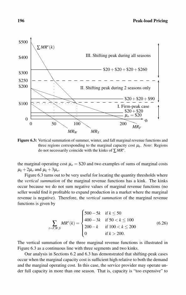
196 Peak-load Pricing
0 20010050
���������
���������������
MRW MRS
$300
$200
$100
��������������������������� qt
MRF
�
$400
$500
0μo = $20
����������������
$20+$20+$90
II. Shifting peak during 2 seasons only
III. Shifting peak during all seasons
$250
�
�
�
$20+$20+$20+$260
∑MRv(k)
I. Firm-peak case$20+$20
Figure 6.3: Vertical summation of summer, winter, and fall marginal revenue functions and
three regions corresponding to the marginal capacity cost μk. Note: Regions
do not necessarily coincide with the kinks of ∑MRv.
the marginal operating cost μo = $20 and two examples of sums of marginal costs
μk +2μo and μk +3μo.
Figure 6.3 turns out to be very useful for locating the quantity thresholds where
the vertical summation of the marginal revenue functions has a kink. The kinks
occur because we do not sum negative values of marginal revenue functions (no
seller would find it profitable to expand production in a market where the marginal
revenue is negative). Therefore, the vertical summation of the marginal revenue
functions is given by
∑t=F,W,S
MRv(k) =
⎧⎪⎪⎪⎪⎨⎪⎪⎪⎪⎩
500−5k if k ≤ 50
400−3k if 50 < k ≤ 100
200− k if 100 < k ≤ 200
0 if k > 200.
(6.26)
The vertical summation of the three marginal revenue functions is illustrated in
Figure 6.3 as a continuous line with three segments and two kinks.
Our analysis in Sections 6.2 and 6.3 has demonstrated that shifting-peak cases
occur when the marginal capacity cost is sufficient high relative to both the demand
and the marginal operating cost. In this case, the service provider may operate un-
der full capacity in more than one season. That is, capacity is “too expensive” to
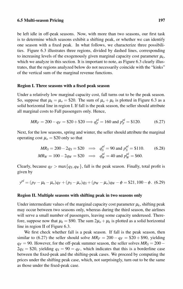
6.5 Multi-season Pricing 197
be left idle in off-peak seasons. Now, with more than two seasons, our first task
is to determine which seasons exhibit a shifting peak, or whether we can identify
one season with a fixed peak. In what follows, we characterize three possibili-
ties. Figure 6.3 illustrates three regions, divided by dashed lines, corresponding
to increasing levels of the exogenously given marginal capacity cost parameter μk,
which we analyze in this section. It is important to note, as Figure 6.3 clearly illus-
trates, that the regions analyzed below do not necessarily coincide with the “kinks”
of the vertical sum of the marginal revenue functions.
Region I. Three seasons with a fixed peak season
Under a relatively low marginal capacity cost, fall turns out to be the peak season.
So, suppose that μk = μo = $20. The sum of μo + μk is plotted in Figure 6.3 as a
solid horizontal line in region I. If fall is the peak season, the seller should attribute
all marginal costs to Fall passengers only. Hence,
MRF = 200−qF = $20+$20 =⇒ qplF = 160 and ppl
F = $120. (6.27)
Next, for the low seasons, spring and winter, the seller should attribute the marginal
operating cost μo = $20 only so that
MRS = 200−2qS = $20 =⇒ qplS = 90 and ppl
S = $110. (6.28)
MRW = 100−2qW = $20 =⇒ qplW = 40 and ppl
W = $60.
Clearly, because qF > max{qS,qW}, fall is the peak season. Finally, total profit is
given by
ypl = (pF −μk−μo)qF +(pS−μo)qS +(pW −μo)qW −φ = $21,100−φ . (6.29)
Region II. Multiple seasons with shifting peak in two seasons only
Under intermediate values of the marginal capacity cost parameter μk, shifting peak
may occur between two seasons only, whereas during the third season, the airlines
will serve a small number of passengers, leaving some capacity underused. There-
fore, suppose now that μk = $90. The sum 2μo + μk is plotted as a solid horizontal
line in region II of Figure 6.3.
We first check whether fall is a peak season. If fall is the peak season, then
similar to (6.27) the seller should solve MRF = 200− qF = $20 + $90, yielding
qF = 90. However, for the off-peak summer season, the seller solves MRS = 200−2qS = $20, yielding qS = 90 = qF , which indicates that this is a borderline case
between the fixed-peak and the shifting-peak cases. We proceed by computing the
prices under the shifting peak case, which, not surprisingly, turn out to be the same
as those under the fixed-peak case.
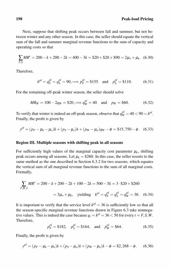
198 Peak-load Pricing
Next, suppose that shifting peak occurs between fall and summer, but not be-
tween winter and any other season. In this case, the seller should equate the vertical
sum of the fall and summer marginal revenue functions to the sum of capacity and
operating costs so that
∑F,S
MRv = 200− k +200−2k = 400−3k = $20+$20+$90 = 2μo + μk. (6.30)
Therefore,
kpl = qplF = qpl
S = 90,=⇒ pplF = $155 and ppl
S = $110. (6.31)
For the remaining off-peak winter season, the seller should solve
MRW = 100−2qW = $20,=⇒ qplW = 40 and pW = $60. (6.32)
To verify that winter is indeed an off-peak season, observe that qplW = 40 < 90 = kpl.
Finally, the profit is given by
ypl = (pF −μk−μo)k +(pS−μo)k +(pW −μo)qW −φ = $15,750−φ . (6.33)
Region III. Multiple seasons with shifting peak in all seasons
For sufficiently high values of the marginal capacity cost parameter μk, shifting
peak occurs among all seasons. Let μk = $260. In this case, the seller resorts to the
same method as the one described in Section 6.3.2 for two seasons, which equates
the vertical sum of all marginal revenue functions to the sum of all marginal costs.
Formally,
∑F,W,S
MRv = 200− k +200−2k +100−2k = 500−5k = 3 ·$20+$260
= 3μo + μk, yielding kpl = qplF = qpl
S = qplW = 36. (6.34)
It is important to verify that the service level kpl = 36 is sufficiently low so that all
the season-specific marginal revenue functions drawn in Figure 6.3 take nonnega-
tive values. This is indeed the case because qt = kpl = 36 < 50 for every t = F,S,W .
Therefore,
pplF = $182, ppl
S = $164, and pplW = $64. (6.35)
Finally, the profit is given by
ypl = (pF −μk−μo)k +(pS−μo)k +(pW −μo)k−φ = $2,268−φ . (6.36)
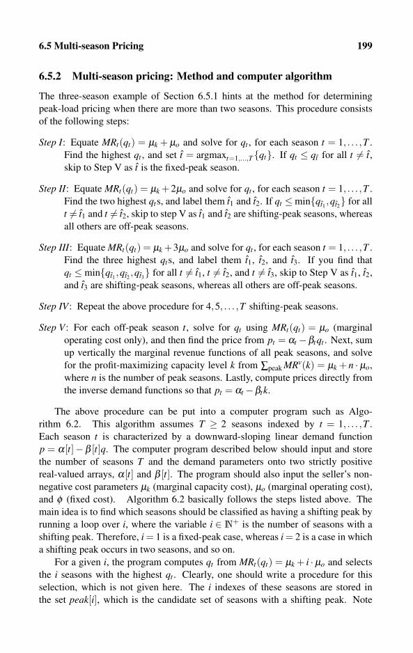
6.5 Multi-season Pricing 199
6.5.2 Multi-season pricing: Method and computer algorithm
The three-season example of Section 6.5.1 hints at the method for determining
peak-load pricing when there are more than two seasons. This procedure consists
of the following steps:
Step I: Equate MRt(qt) = μk + μo and solve for qt , for each season t = 1, . . . ,T .
Find the highest qt , and set t = argmaxt=1,...,T{qt}. If qt ≤ qt for all t �= t,skip to Step V as t is the fixed-peak season.
Step II: Equate MRt(qt) = μk +2μo and solve for qt , for each season t = 1, . . . ,T .
Find the two highest qts, and label them t1 and t2. If qt ≤min{qt1 ,qt2} for all
t �= t1 and t �= t2, skip to step V as t1 and t2 are shifting-peak seasons, whereas
all others are off-peak seasons.
Step III: Equate MRt(qt) = μk +3μo and solve for qt , for each season t = 1, . . . ,T .
Find the three highest qts, and label them t1, t2, and t3. If you find that
qt ≤min{qt1 ,qt2 ,qt3} for all t �= t1, t �= t2, and t �= t3, skip to Step V as t1, t2,
and t3 are shifting-peak seasons, whereas all others are off-peak seasons.
Step IV: Repeat the above procedure for 4,5, . . . ,T shifting-peak seasons.
Step V: For each off-peak season t, solve for qt using MRt(qt) = μo (marginal
operating cost only), and then find the price from pt = αt −βtqt . Next, sum
up vertically the marginal revenue functions of all peak seasons, and solve
for the profit-maximizing capacity level k from ∑peak MRv(k) = μk + n · μo,
where n is the number of peak seasons. Lastly, compute prices directly from
the inverse demand functions so that pt = αt −βtk.
The above procedure can be put into a computer program such as Algo-
rithm 6.2. This algorithm assumes T ≥ 2 seasons indexed by t = 1, . . . ,T .
Each season t is characterized by a downward-sloping linear demand function
p = α[t]−β [t]q. The computer program described below should input and store
the number of seasons T and the demand parameters onto two strictly positive
real-valued arrays, α[t] and β [t]. The program should also input the seller’s non-
negative cost parameters μk (marginal capacity cost), μo (marginal operating cost),
and φ (fixed cost). Algorithm 6.2 basically follows the steps listed above. The
main idea is to find which seasons should be classified as having a shifting peak by
running a loop over i, where the variable i ∈ N+ is the number of seasons with a
shifting peak. Therefore, i = 1 is a fixed-peak case, whereas i = 2 is a case in which
a shifting peak occurs in two seasons, and so on.
For a given i, the program computes qt from MRt(qt) = μk + i · μo and selects
the i seasons with the highest qt . Clearly, one should write a procedure for this
selection, which is not given here. The i indexes of these seasons are stored in
the set peak[i], which is the candidate set of seasons with a shifting peak. Note
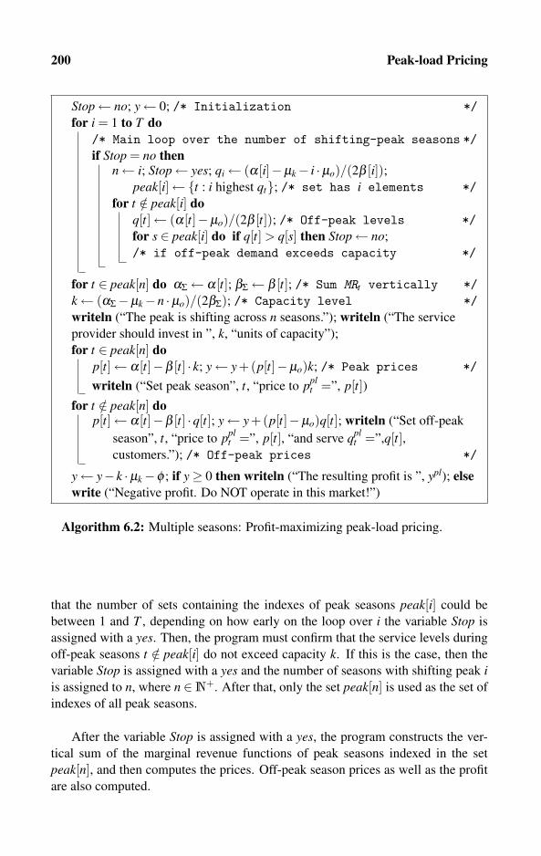
200 Peak-load Pricing
Stop← no; y← 0; /* Initialization */for i = 1 to T do
/* Main loop over the number of shifting-peak seasons */if Stop = no then
n← i; Stop← yes; qi← (α[i]−μk− i ·μo)/(2β [i]);peak[i]←{t : i highest qt}; /* set has i elements */
for t /∈ peak[i] doq[t]← (α[t]−μo)/(2β [t]); /* Off-peak levels */for s ∈ peak[i] do if q[t] > q[s] then Stop← no;
/* if off-peak demand exceeds capacity */
for t ∈ peak[n] do αΣ← α[t]; βΣ← β [t]; /* Sum MRt vertically */k← (αΣ−μk−n ·μo)/(2βΣ); /* Capacity level */writeln (“The peak is shifting across n seasons.”); writeln (“The service
provider should invest in ”, k, “units of capacity”);
for t ∈ peak[n] dop[t]← α[t]−β [t] · k; y← y+(p[t]−μo)k; /* Peak prices */
writeln (“Set peak season”, t, “price to pplt =”, p[t])
for t /∈ peak[n] dop[t]← α[t]−β [t] ·q[t]; y← y+(p[t]−μo)q[t]; writeln (“Set off-peak
season”, t, “price to pplt =”, p[t], “and serve qpl
t =”,q[t],customers.”); /* Off-peak prices */
y← y− k ·μk−φ ; if y≥ 0 then writeln (“The resulting profit is ”, ypl); elsewrite (“Negative profit. Do NOT operate in this market!”)
Algorithm 6.2: Multiple seasons: Profit-maximizing peak-load pricing.
that the number of sets containing the indexes of peak seasons peak[i] could be
between 1 and T , depending on how early on the loop over i the variable Stop is
assigned with a yes. Then, the program must confirm that the service levels during
off-peak seasons t /∈ peak[i] do not exceed capacity k. If this is the case, then the
variable Stop is assigned with a yes and the number of seasons with shifting peak iis assigned to n, where n ∈N+. After that, only the set peak[n] is used as the set of
indexes of all peak seasons.
After the variable Stop is assigned with a yes, the program constructs the ver-
tical sum of the marginal revenue functions of peak seasons indexed in the set
peak[n], and then computes the prices. Off-peak season prices as well as the profit
are also computed.
6.6 Season-interdependent Demand Functions 201
6.6 Season-interdependent Demand Functions
Our analysis so far was based on the assumption that the demand for service in each
season is independent of how the service is priced in all other seasons. However,
in reality, for some consumers the demand functions are interdependent, which
means that a reduction in price during one season may cause some consumers to
postpone or advance their service demand to the “discounted” season. For exam-
ple, friends tend to delay long phone conversations to off-peak hours, including
late-night hours, weekends, and holidays, because these time periods are heavily
discounted. Also, people tend to postpone or advance their nonbusiness trips to
travel during discounted off-peak seasons. In both examples, if the service provider
charges uniform prices in all seasons, most consumers may demand the service dur-
ing the peak-season only.
In the literature, there are several formulations that introduce substitution
among seasons. Crew and Kleindorfer (1986, Sec. 3.4), following Dansby (1975),
allow for nonzero cross-derivatives of a season’s demand function with respect to
output sold in different seasons. Bergstrom and MacKie-Mason (1991) and Shy
(1996, Ch. 13) allow for substitution between seasons in utility-based models.
6.6.1 Winters and summers: An example
To capture consumer substitution across seasons, we slightly modify the example
of a small airline, LUFTPAPA. More precisely, we transform the system of inde-
pendent seasonal demand functions (6.1) into the interdependent inverse demand
functions given by
pS = αS−βSqS− γSqW = 200−qS−0.2qW , (6.37)
pW = αW −βW qW − γW qS = 100−qW −0.2qS.
The system of demand functions formulated in (6.37) implies that winter service
and summer service are substitutes to some degree. Here, an increase in the number
of passengers who fly over the winter will reduce passengers’ willingness to pay in
both seasons. The same applies for an increase in the number of passengers who fly
over the summer. This is what makes the service in both seasons substitute goods
(see Definition 2.4 for the direct demand case).
Next, the seasonal total revenue functions associated with the demand functions
(6.37) are
xS(qS,qW ) = (200−qS−0.2qW )qS, (6.38)
xW (qS,qW ) = (100−qW −0.2qS)qW .
Notice that the revenue generated in each season now depends on the level of ser-
vice provided in all seasons because the seasonal demand functions (6.37) are in-
terdependent. Thus, instead of deriving only two marginal revenue functions, one

202 Peak-load Pricing
for each market, we now must derive four marginal revenue functions defined by
MRSSdef=
∂xS
∂qS= 200−2qS−0.2qW ,
MRSWdef=
∂xS
∂qW=−0.2qS, (6.39)
MRWWdef=
∂xW
∂qW= 100−2qW −0.2qS,
MRWSdef=
∂xW
∂qS=−0.2qW .
The newly defined cross-marginal revenue function MRSW measures the change in
revenue during the summer generated by a “small” increase in service level dur-
ing the winter. Similarly, the cross-marginal revenue function MRWS measures the
change in revenue during the winter generated by a “small” increase in service level
during the summer.
Interdependent demand airline example: Fixed-peak case
Suppose that LUFTPAPA’s cost parameters are now given by μk = μo = $20 and
φ = $2000. We basically follow the same steps as in Section 6.2.2, except that
now four marginal revenue functions enter the calculations instead of only two. We
first assume (and later verify) that summer is the peak season. In this case, the
seller should solve for the summer and winter service levels qS and qW using the
following two conditions:
MRSS +MRWS = 200−2qS−0.2qW −0.2qW = $20+$20 = μk + μo,
MRWW +MRSW = 100−2qW −0.2qS−0.2qS = $20 = μo. (6.40)
The top equation equates the sum of summer and winter’s marginal revenues as-
sociated with a small expansion of service during the summer, to the sum of all
marginal costs. The bottom condition equates the sum of marginal revenue func-
tions associated with a small increase in the service level during the winter to the
marginal operating cost only. Solving (6.40) for service levels qS and qW and then
substituting these into the inverse demand functions (6.37) yield
kpl = qplS = 75, qpl
W = 25, pplS = $120, and ppl
W = $51. (6.41)
This confirms that summer is indeed the peak season. Comparing the prices (6.41)
with the prices computed under independent seasonal demand (6.4) reveals that
when demand functions are interdependent, the seller lowers the price during the
low season (Winter in the present example). Lowering the off-peak price is done
for the purpose of trying to make passengers switch from the peak season to the
6.6 Season-interdependent Demand Functions 203
lower season. Finally, for the sake of completeness, the total profit earned by the
seller by using the above peak-load pricing is
ypl = (pS−μk−μo)qS +(pW −μo)qW −φ = $4775. (6.42)
Interdependent demand airline example: Shifting-peak case
Suppose that LUFTPAPA’s cost parameters are now given by μk = $160, μo = $20,
and φ = $1000. We basically follow the same steps as in Section 6.3.2, except that
now we have four marginal revenue functions given by (6.39) instead of only two.
To demonstrate that summer is not a peak season, we investigate conditions
(6.40) under the new cost structure. Hence,
MRSS +MRWS = 200−2qS−0.2qW −0.2qW = $160+$20 = μk + μo,
MRWW +MRSW = 100−2qW −0.2qS−0.2qS = $20 = μo, (6.43)
yielding qS = 25/12 < 475/12 = qW . Thus, summer is not a peak season. Clearly,
using the same method, we can show that winter is also not a peak season, which
implies that the shifting-peak case applies.
Under the shifting-peak case, the airline serves at full capacity in both seasons
so that k = qS = qW . Equating the vertical sum of the four marginal revenue func-
tions at full capacity to the sum of marginal capacity and operating costs yields
∑S,W
MRv(k) = 300− 24k5
= $160+$20+$20 = μk +2μo,
yielding kpl = qplS = qpl
W =125
6. (6.44)
Therefore,
pplS = 200− kpl−0.2kpl = $175 and ppl
W = 100− kpl−0.2kpl = $75. (6.45)
Finally, for the sake of completeness, the total profit earned by the seller by using
the above peak-load pricing is
ypl = (pS−μk−μo)kpl +(pW −μo)kpl−φ =3125
3−1000 =
125
3. (6.46)
6.6.2 Interdependent demand: General formulation
We now extend the airline example of Section 6.6.1 to general demand functions
as specified in (6.37). As explained in Section 2.7 (for the direct demand case),
the parameters of this system of inverse demand functions αS, αW , βS, βW , γS,
and γW can be estimated from past data on seasonal prices and the number of
served passengers. It must be verified that the estimated demand parameters satisfy
204 Peak-load Pricing
min{βS,βW} > max{γS,γW}, which means that a season’s price is more sensitive
to variations in the service of the same season relative to the variation in the service
level during other seasons. Economists often state this condition by saying that the
“own” effect is stronger than the substitute effect.
The demand functions (6.37) yield the revenue functions
xS(qS,qW ) = (αS−βSqS− γSqW )qS, (6.47)
xW (qS,qW ) = (αW −βW qW − γW qS)qW .
The corresponding four marginal revenue functions are therefore given by
MRSSdef=
∂xS
∂qS= αS−2βSqS− γSqW ,
MRSWdef=
∂xS
∂qW=−γSqS, (6.48)
MRWWdef=
∂xW
∂qW= αW −2βW qW − γW qS,
MRWSdef=
∂xW
∂qS=−γW qW .
Interdependent demand general formulation: Fixed-peak case
Assuming first (and verifying later) that summer is a peak season, the seller deter-
mines the amount of service qS and qW by solving
MRSS +MRWS = αS−2βSqS− γSqW − γW qW = μk + μo,
MRWW +MRSW = aW −2βW qW − γW qS− γSqS = μo, (6.49)
yielding the service levels
qplS =
2αSβW −αW (γS + γW )−2βW (μk + μo)+(γS + γW )μo
4βSβW − (γS + γW )2, (6.50)
qplW =
2αW βS−αS(γS + γW )−2βSμo +(γS + γW )(μk + μo)4βSβW − (γS + γW )2
.
At this stage, it should be verified that kpl = qplS > qpl
W , meaning that summer is
indeed a peak season. Finally, the profit-maximizing seasonal prices pplS and ppl
Ware computed by substituting the service levels (6.50) into the system of inverse
demand functions (6.37). The profit is then found by substituting the service levels
and prices into the profit function (6.42).
6.7 Regulated Public Utility 205
Interdependent demand general formulation: Shifting-peak case
The seller should equate the vertical sum of the four marginal revenue functions at
full capacity to the sum of marginal capacity and operating costs so that
∑S,W
MRv(k) = αS +αW −2(βS +βW + γS + γW )k = μk +2μo. (6.51)
Setting k = qS = qW yields the desired capacity level
k = qS = qW =αS +αW −μk−2μo
2(βS +βW + γS + γW ). (6.52)
Finally, the profit-maximizing seasonal prices pplS and ppl
W are computed by sub-
stituting the capacity level from (6.52) into the system of inverse demand functions
(6.37). The profit is then found by substituting the service levels and prices into the
profit function (6.46).
6.7 Regulated Public Utility
The difference between a regulator of a public utility and a profit-maximizing firm
is that a regulator is concerned with consumer welfare and industry profit, whereas
a firm seeks to maximize profit only. The regulator often sets prices to maximize
a social welfare function, which for the present formulation (with no fixed costs)
boils down to maximizing consumer welfare subject to the constraint that the firm
break even (hence does not make any loss). The objective of a regulator of a public
utility has been discussed earlier in this book (see Sections 3.6.2 and 5.5). There-
fore, we confine the analysis of this section to modifying the monopoly seller’s
algorithm for determining peak-load pricing to an algorithm for regulating public
utilities.
The main difference between the algorithms used by a profit-maximizing sin-
gle seller and those employed by the regulator is that a regulator tends to equate the
prices to the “relevant” marginal costs, as opposed to a monopoly firm that devi-
ates from marginal cost pricing by equating the marginal revenue to the “relevant”
marginal cost, thereby restricting its output. However, marginal cost pricing would
generate a loss to the seller as marginal cost pricing will not generate any revenue
that may be needed to cover the fixed cost φ . For this reason, our analysis here is
limited to the case in which the fixed costs are either nonexisting or are financed
by the taxpayers. It should be noted that if fixed costs were present, the regulator
could use two-part tariffs whereby the fixed fees levied on consumers could be used
for financing the seller’s fixed cost (see Section 5.5). Alternatively, in the presence
of fixed costs, the regulator could deviate from marginal cost pricing according to
the Ramsey principle as explained in Section 3.6.2.
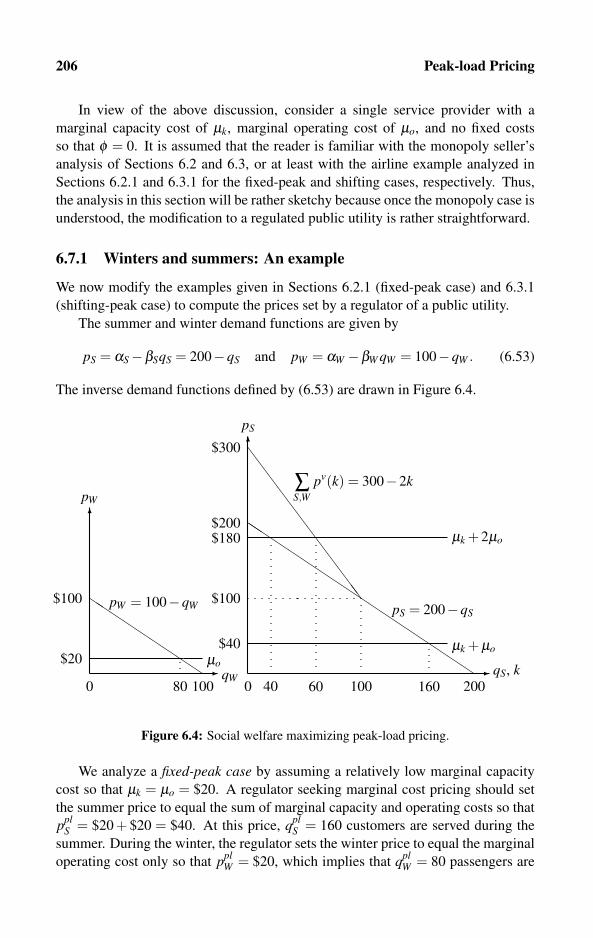
206 Peak-load Pricing
In view of the above discussion, consider a single service provider with a
marginal capacity cost of μk, marginal operating cost of μo, and no fixed costs
so that φ = 0. It is assumed that the reader is familiar with the monopoly seller’s
analysis of Sections 6.2 and 6.3, or at least with the airline example analyzed in
Sections 6.2.1 and 6.3.1 for the fixed-peak and shifting cases, respectively. Thus,
the analysis in this section will be rather sketchy because once the monopoly case is
understood, the modification to a regulated public utility is rather straightforward.
6.7.1 Winters and summers: An example
We now modify the examples given in Sections 6.2.1 (fixed-peak case) and 6.3.1
(shifting-peak case) to compute the prices set by a regulator of a public utility.
The summer and winter demand functions are given by
pS = αS−βSqS = 200−qS and pW = αW −βW qW = 100−qW . (6.53)
The inverse demand functions defined by (6.53) are drawn in Figure 6.4.
�������������������
0 200
$40 μk + μo
�
�
���
��
��
��
0
pW
$100
100
$20 μoqW
pW = 100−qW $100pS = 200−qS
�$300
pS
16080
$200
100
������������
$180 μk +2μo
60
∑S,W
pv(k) = 300−2k
qS, k40
Figure 6.4: Social welfare maximizing peak-load pricing.
We analyze a fixed-peak case by assuming a relatively low marginal capacity
cost so that μk = μo = $20. A regulator seeking marginal cost pricing should set
the summer price to equal the sum of marginal capacity and operating costs so that
pplS = $20 + $20 = $40. At this price, qpl
S = 160 customers are served during the
summer. During the winter, the regulator sets the winter price to equal the marginal
operating cost only so that pplW = $20, which implies that qpl
W = 80 passengers are
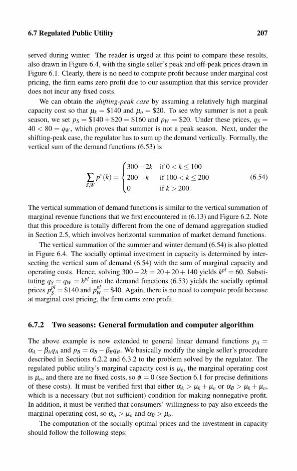
6.7 Regulated Public Utility 207
served during winter. The reader is urged at this point to compare these results,
also drawn in Figure 6.4, with the single seller’s peak and off-peak prices drawn in
Figure 6.1. Clearly, there is no need to compute profit because under marginal cost
pricing, the firm earns zero profit due to our assumption that this service provider
does not incur any fixed costs.
We can obtain the shifting-peak case by assuming a relatively high marginal
capacity cost so that μk = $140 and μo = $20. To see why summer is not a peak
season, we set pS = $140 + $20 = $160 and pW = $20. Under these prices, qS =40 < 80 = qW , which proves that summer is not a peak season. Next, under the
shifting-peak case, the regulator has to sum up the demand vertically. Formally, the
vertical sum of the demand functions (6.53) is
∑S,W
pv(k) =
⎧⎪⎨⎪⎩
300−2k if 0 < k ≤ 100
200− k if 100 < k ≤ 200
0 if k > 200.
(6.54)
The vertical summation of demand functions is similar to the vertical summation of
marginal revenue functions that we first encountered in (6.13) and Figure 6.2. Note
that this procedure is totally different from the one of demand aggregation studied
in Section 2.5, which involves horizontal summation of market demand functions.
The vertical summation of the summer and winter demand (6.54) is also plotted
in Figure 6.4. The socially optimal investment in capacity is determined by inter-
secting the vertical sum of demand (6.54) with the sum of marginal capacity and
operating costs. Hence, solving 300−2k = 20+20+140 yields kpl = 60. Substi-
tuting qS = qW = kpl into the demand functions (6.53) yields the socially optimal
prices pplS = $140 and ppl
W = $40. Again, there is no need to compute profit because
at marginal cost pricing, the firm earns zero profit.
6.7.2 Two seasons: General formulation and computer algorithm
The above example is now extended to general linear demand functions pA =αA−βAqA and pB = αB−βBqB. We basically modify the single seller’s procedure
described in Sections 6.2.2 and 6.3.2 to the problem solved by the regulator. The
regulated public utility’s marginal capacity cost is μk, the marginal operating cost
is μo, and there are no fixed costs, so φ = 0 (see Section 6.1 for precise definitions
of these costs). It must be verified first that either αA > μk + μo or αB > μk + μo,
which is a necessary (but not sufficient) condition for making nonnegative profit.
In addition, it must be verified that consumers’ willingness to pay also exceeds the
marginal operating cost, so αA > μo and αB > μo.
The computation of the socially optimal prices and the investment in capacity
should follow the following steps:

208 Peak-load Pricing
Step I: Check if A is the peak season by setting pplA = αA− βAqA = μk + μo and
pplB = αB−βBqB = μo to obtain
qplA =
αA−μk−μo
βAand qpl
B =αB−μo
βB. (6.55)
Now, check if A is indeed the peak season so that qplB ≤ qpl
A . If this is the case,
then set the capacity level to kpl = qplA and stop here.
Step II: Check if B is the peak season by setting pplB = αB−βBqB = μk + μo and
pplA = αA−βAqA = μo to obtain
qplB =
αB−μk−μo
βBand qpl
A =αA−μo
βA. (6.56)
Now, check if B is indeed the peak season so that qplA ≤ qpl
B . If this is the case,
then set the capacity level to kpl = qplB and stop here. If this is not the case
continue to Step III as you have reached the shifting-peak case.
Step III: Sum up vertically the two demand functions and equate this sum to the
sum of marginal capacity and marginal operating costs
∑A,B
pv(k) = αA +αB− (βA +βB)k = μk +2μo, (6.57)
which obtains the desired capacity level
kpl = qplA = qpl
B =αA +αB−μk−2μo
βA +βB. (6.58)
Step IV: Substitute kpl = qplA = qpl
B into each demand function to obtain the price in
each season
pplA =
αAβB−βA(αB−μk−2μo)βA +βB
, (6.59)
pplB =
αBβA−βB(αA−μk−2μo)βA +βB
.
Using the steps listed above, we now modify Algorithm 6.1, designed for max-
imizing profit, to an algorithm used by a regulator seeking to maximize social wel-
fare. Note that this algorithm is valid as long as there are no fixed costs, φ = 0.
The explanation of Algorithm 6.3 and the variable inputting required for running
this program are very much the same as the ones described for Algorithm 6.1 and
therefore will not be repeated here.

6.7 Regulated Public Utility 209
peak← 0; off← 0; /* Initialization */if (α[1]−μk−μo)/β [1]≥ (α[2]−μo)/β [2] then
peak← 1; off← 2; /* Season 1 is peak, 2 is off-peak */
if (α[2]−μk−μo)/β [2]≥ (α[1]−μo)/β [1] thenpeak← 2; off← 1; /* Season 2 is peak, 1 is off-peak */
if peak �= 0 then/* Fixed-peak case */p[peak]← μk + μo; q[peak]← (α[peak]−μk−μo)/β [peak];p[off]← μo; q[off]← (α[off]−μo)/β [off]; writeln (peak,“ is the peak
season, and the seller should invest in kpl = ”, q[peak], “ units of
capacity.”); writeln (“The peak season price should be set to ”, p[peak],“The off-peak season price should be set to ”, p[off]); writeln (“The
peak season demand equals full capacity, q[peak], “The off-peak season
demand is ”, q[off]);if peak = 0 then
/* Shifting-peak case */k← (α[1]+α[2]−μk−2μo)/(β [1]+β [2]); p[1]← α[1]−β [1]k;
p[2]← α[2]−β [2]k; ypl← (p[1]−μk−μo)k +(p[2]−μo)k−φ ;
writeln (“Shifting peak case so q[1] = q[2] = kpl. The seller should
invest in kpl = ”, k, “ units of capacity.”); writeln (“The price in season 1
should be set to ”, p[1], “and in season 2 to ”, p[2]);
Algorithm 6.3: Two seasons: Welfare-maximizing peak-load pricing.
6.7.3 Multi-season pricing: A three-season example
We now modify the three-season analysis of Section 6.5.1 to apply to a pricing de-
cision made by a welfare-maximizing regulator, instead of by a profit-maximizing
service provider. This modification is rather simple as it basically involves chang-
ing to marginal cost pricing instead of equating marginal revenues to marginal
costs, and therefore will be presented here without extensive discussions. Simi-
lar to Section 6.5.1, suppose that the demand functions during summer, winter, and
fall are given by
pS = 200−qS, pW = 100−qW , and pF = 200− qF
2. (6.60)
Figure 6.5 depicts the three demand functions (6.60). Figure 6.5 also plots the
marginal operating cost μo = $20 and two examples of sums of marginal capacity
and operating costs.
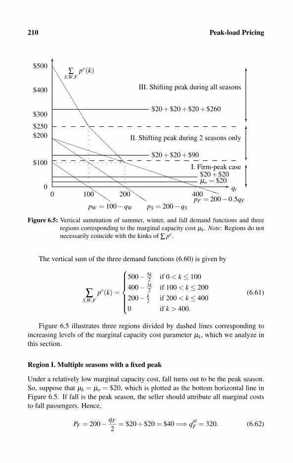
210 Peak-load Pricing
0 400200100
���������
���������������
pW = 100−qW pS = 200−qS
$300
$200
$100
��������������������������� qt
pF = 200−0.5qF
�
$400
$500
0μo = $20
����������������
�
�
�
II. Shifting peak during 2 seasons only
III. Shifting peak during all seasons
$250
$20+$20+$20+$260
$20+$20+$90
∑S,W,F
pv(k)
I. Firm-peak case$20+$20
Figure 6.5: Vertical summation of summer, winter, and fall demand functions and three
regions corresponding to the marginal capacity cost μk. Note: Regions do not
necessarily coincide with the kinks of ∑ pv.
The vertical sum of the three demand functions (6.60) is given by
∑S,W,F
pv(k) =
⎧⎪⎪⎪⎪⎨⎪⎪⎪⎪⎩
500− 5k2
if 0 < k ≤ 100
400− 3k2
if 100 < k ≤ 200
200− k2
if 200 < k ≤ 400
0 if k > 400.
(6.61)
Figure 6.5 illustrates three regions divided by dashed lines corresponding to
increasing levels of the marginal capacity cost parameter μk, which we analyze in
this section.
Region I. Multiple seasons with a fixed peak
Under a relatively low marginal capacity cost, fall turns out to be the peak season.
So, suppose that μk = μo = $20, which is plotted as the bottom horizontal line in
Figure 6.5. If fall is the peak season, the seller should attribute all marginal costs
to fall passengers. Hence,
PF = 200− qF
2= $20+$20 = $40 =⇒ qpl
F = 320. (6.62)

6.7 Regulated Public Utility 211
Next, for the off-peak seasons spring and winter, the seller should attribute the
marginal operating cost μo = $20 only so that
pS = 200−qS = $20 =⇒ qplS = 180, (6.63)
pW = 100−qW = $20 =⇒ qplW = 80.
Clearly, fall is the peak season because qplF > max{qpl
S ,qplW}.
Region II. Multiple seasons with shifting peak in two seasons only
Under intermediate values of the marginal capacity cost μk, shifting peak may occur
between two seasons only, whereas the third season will serve a small number of
customers with no shifting peak. Therefore, suppose now that μk = $90. The sum
μo + μk is plotted as a solid horizontal line in Region II of Figure 6.5.
We first check whether fall is a peak season. If fall is the peak season, then the
seller should solve pF = 200− qF/2 = $20 + $90, yielding qF = 180. However,
during the off-peak summer season, the seller solves pS = 200−qS = $20, yielding
qS = 180 = qF , implying that this is a borderline case between the fixed- and shift-
peak cases. We proceed by solving it as a shifting-peak case, which should yield
the same result as solving it under the fixed-peak case.
Next, suppose that shifting peak occurs between fall and summer, but not be-
tween winter and any other season. In this case, the seller should equate the vertical
sum of the fall and winter demand to the sum of capacity and operating costs so
that
∑F,S
pv(k) = 200− k2
+200−k = 400− 3k2
= $20+$20+$90 = 2μo + μk. (6.64)
Therefore,
kpl = qplF = qpl
S = 180, hence pplF = $110 and ppl
S = $20. (6.65)
For the remaining off-peak winter season, the seller should solve
pW = 100−qW = $20 =⇒ qplW = 80. (6.66)
To verify that winter is indeed an off-peak season, observe that qplW = 80 < 180 =
kpl.
Region III. Multiple seasons with shifting peak in all seasons
For sufficiently high values of the marginal capacity cost parameter μk, shifting
peak occurs among all seasons. In this case, the seller equates the vertical sum of
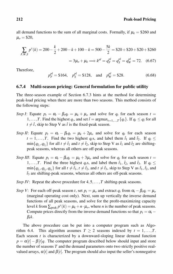
212 Peak-load Pricing
all demand functions to the sum of all marginal costs. Formally, if μk = $260 and
μo = $20,
∑F,W,S
pv(k) = 200− k2
+200−k+100−k = 500− 5k2
= $20+$20+$20+$260
= 3μo + μk =⇒ kpl = qplF = qpl
S = qplW = 72. (6.67)
Therefore,
pplF = $164, ppl
S = $128, and pplW = $28. (6.68)
6.7.4 Multi-season pricing: General formulation for public utility
The three-season example of Section 6.7.3 hints at the method for determining
peak-load pricing when there are more than two seasons. This method consists of
the following steps:
Step I: Equate pt = αt − βtqt = μk + μo and solve for qt for each season t =1, . . . ,T . Find the highest qt , and set t = argmaxt=1,...,T{qt}. If qt ≤ qt for all
t �= t, skip to Step V as t is the fixed-peak season.
Step II: Equate pt = αt − βtqt = μk + 2μo and solve for qt for each season
t = 1, . . . ,T . Find the two highest qts, and label them t1 and t2. If qt ≤min{qt1 ,qt2} for all t �= t1 and t �= t2, skip to Step V as t1 and t2 are shifting-
peak seasons, whereas all others are off-peak seasons.
Step III: Equate pt = αt − βtqt = μk + 3μo and solve for qt for each season t =1, . . . ,T . Find the three highest qts, and label them t1, t2, and t3. If qt ≤min{qt1 ,qt2 ,qt3} for all t �= t1, t �= t2, and t �= t3, skip to Step V as t1, t2, and
t3 are shifting-peak seasons, whereas all others are off-peak seasons.
Step IV: Repeat the above procedure for 4,5, . . . ,T shifting-peak seasons.
Step V: For each off-peak season t, set pt = μo and extract qt from αt −βtqt = μo
(marginal operating cost only). Next, sum up vertically the inverse demand
functions of all peak seasons, and solve for the profit-maximizing capacity
level k from ∑peak pv(k) = μk +n ·μo, where n is the number of peak seasons.
Compute prices directly from the inverse demand functions so that pt = αt−βtk.
The above procedure can be put into a computer program such as Algo-
rithm 6.4. This algorithm assumes T ≥ 2 seasons indexed by t = 1, . . . ,T .
Each season t is characterized by a downward-sloping linear demand function
p = α[t]−β [t]q. The computer program described below should input and store
the number of seasons T and the demand parameters onto two strictly positive real-
valued arrays, α[t] and β [t]. The program should also input the seller’s nonnegative
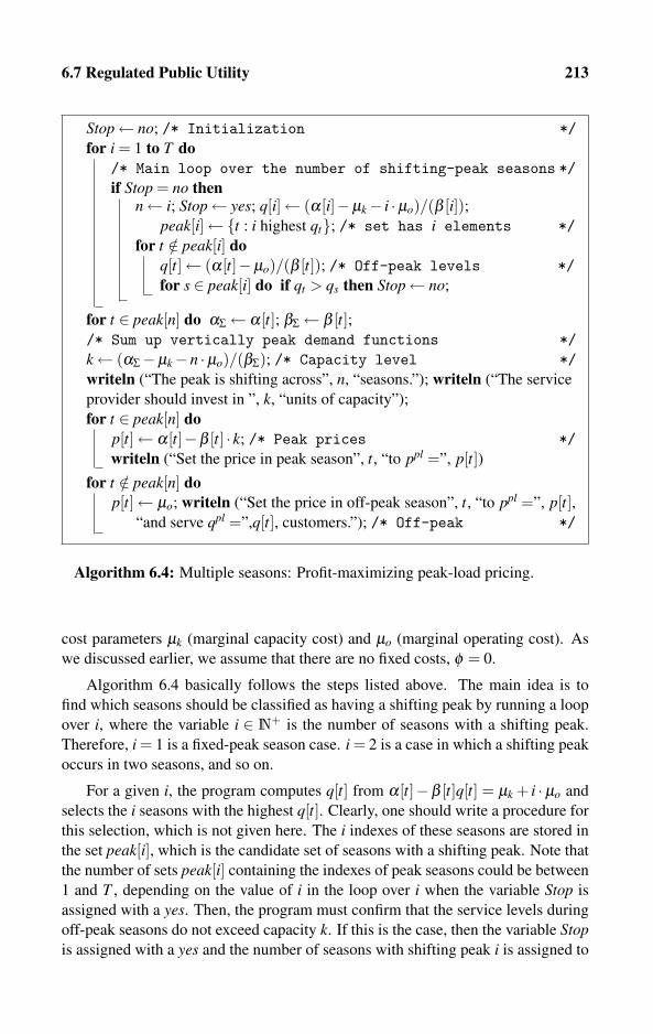
6.7 Regulated Public Utility 213
Stop← no; /* Initialization */for i = 1 to T do
/* Main loop over the number of shifting-peak seasons */if Stop = no then
n← i; Stop← yes; q[i]← (α[i]−μk− i ·μo)/(β [i]);peak[i]←{t : i highest qt}; /* set has i elements */
for t /∈ peak[i] doq[t]← (α[t]−μo)/(β [t]); /* Off-peak levels */for s ∈ peak[i] do if qt > qs then Stop← no;
for t ∈ peak[n] do αΣ← α[t]; βΣ← β [t];/* Sum up vertically peak demand functions */k← (αΣ−μk−n ·μo)/(βΣ); /* Capacity level */writeln (“The peak is shifting across”, n, “seasons.”); writeln (“The service
provider should invest in ”, k, “units of capacity”);
for t ∈ peak[n] dop[t]← α[t]−β [t] · k; /* Peak prices */writeln (“Set the price in peak season”, t, “to ppl =”, p[t])
for t /∈ peak[n] dop[t]← μo; writeln (“Set the price in off-peak season”, t, “to ppl =”, p[t],
“and serve qpl =”,q[t], customers.”); /* Off-peak */
Algorithm 6.4: Multiple seasons: Profit-maximizing peak-load pricing.
cost parameters μk (marginal capacity cost) and μo (marginal operating cost). As
we discussed earlier, we assume that there are no fixed costs, φ = 0.
Algorithm 6.4 basically follows the steps listed above. The main idea is to
find which seasons should be classified as having a shifting peak by running a loop
over i, where the variable i ∈ N+ is the number of seasons with a shifting peak.
Therefore, i = 1 is a fixed-peak season case. i = 2 is a case in which a shifting peak
occurs in two seasons, and so on.
For a given i, the program computes q[t] from α[t]−β [t]q[t] = μk + i · μo and
selects the i seasons with the highest q[t]. Clearly, one should write a procedure for
this selection, which is not given here. The i indexes of these seasons are stored in
the set peak[i], which is the candidate set of seasons with a shifting peak. Note that
the number of sets peak[i] containing the indexes of peak seasons could be between
1 and T , depending on the value of i in the loop over i when the variable Stop is
assigned with a yes. Then, the program must confirm that the service levels during
off-peak seasons do not exceed capacity k. If this is the case, then the variable Stopis assigned with a yes and the number of seasons with shifting peak i is assigned to
214 Peak-load Pricing
the n, where n ∈N+. After that, only the set peak[n] is used as the set of indexes of
all peak seasons.
Once the variable Stop is assigned with a yes, the program constructs the ver-
tical sum of the marginal revenue functions of all peak seasons then computes the
prices. Lastly, off-peak season prices as well as the profit are also computed.
6.8 Demand, Cost, and the Lengths of Seasons
Our analysis has so far abstracted from analyzing the precise relationship among
the specification of demand functions, the cost of investing in capacity, and the
duration of each season. To see why improper specification of these may result
in computation errors, consider the LUFTPAPA Airlines example of Sections 6.2.1
and 6.3.1, where qS and qW denote the total number of passengers during the sum-
mer and winter, respectively. We have shown that if summer is a fixed-peak season,
the airline invests in k = qS ≥ qW units of capacity. However, this result may be
falsely interpreted that this airlines maintains a capacity level that enables it to serve
qS passengers at each moment in time. For example, if the airline serves 2 million
passengers, our specification implies that this airline has the potential of flying 2
million passengers at the same time on its existing fleet of aircraft. If the aver-
age aircraft capacity is 200 passengers, this interpretation implies that LUFTPAPA
Airlines must acquire 10,000 airplanes, which is impossible.
The above-mentioned inconsistency can also be demonstrated by looking at
electrical power plants. If consumers of electricity use a few billion of kilowatt-
hours of electricity in a given season, this does not imply that the power plant
should maintain a capacity of this magnitude at each hour during this season.
In this case, what matters is whether the electric company invests in a sufficient
amount of capacity that would enable it to supply the flow of electricity demanded
at each point in time. These issues have been carefully investigated by Wilson
(1972), who reconciled the Steiner (1957) approach, used so far in this book, with
Williamson (1966), who proposed a solution to peak-load pricing with seasons of
unequal lengths.
A successful implementation of profitable peak-load pricing schemes depends
on proper definitions of the duration of service, the lengths of seasons and cycles,
and the marginal capacity and operating costs. These definitions must be consis-
tent with respect to their time dimension, as we demonstrate in Table 6.3. Table 6.3
demonstrates that before any analysis of peak-load pricing (in fact, before setting
any price) the seller must specify the duration upon which the service is measured.
In Table 6.3, electricity is measured in kilowatt-hours, which is the standard mea-
sure used by all electric companies. Then, μo is the operating cost associated with
increasing electricity output by one kilowatt-hour. Notice that services are gener-
ally classified as flow goods, which means that once they are consumed, they must
be reproduced for additional consumption. Thus, μo should also be treated as a
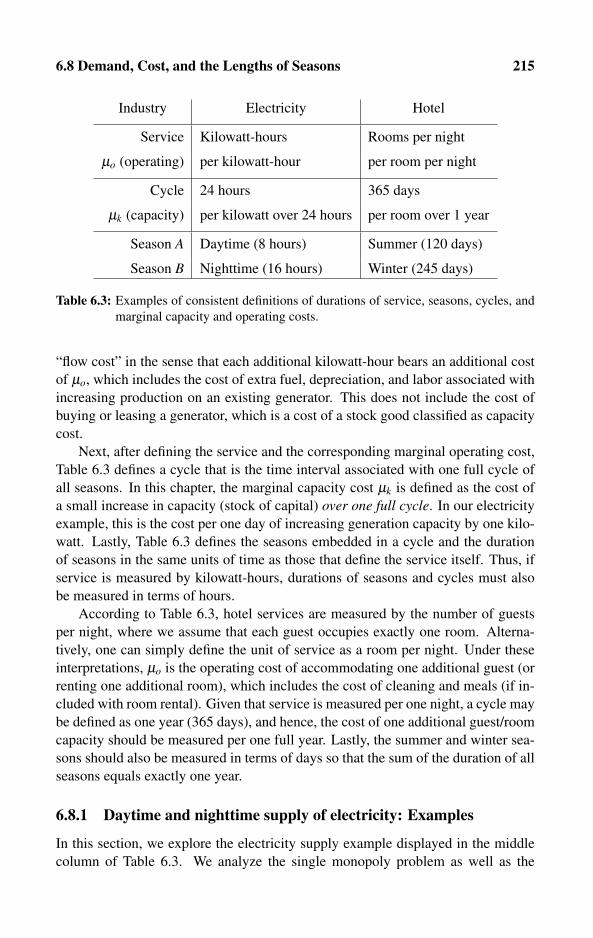
6.8 Demand, Cost, and the Lengths of Seasons 215
Industry Electricity Hotel
Service Kilowatt-hours Rooms per night
μo (operating) per kilowatt-hour per room per night
Cycle 24 hours 365 days
μk (capacity) per kilowatt over 24 hours per room over 1 year
Season A Daytime (8 hours) Summer (120 days)
Season B Nighttime (16 hours) Winter (245 days)
Table 6.3: Examples of consistent definitions of durations of service, seasons, cycles, and
marginal capacity and operating costs.
“flow cost” in the sense that each additional kilowatt-hour bears an additional cost
of μo, which includes the cost of extra fuel, depreciation, and labor associated with
increasing production on an existing generator. This does not include the cost of
buying or leasing a generator, which is a cost of a stock good classified as capacity
cost.
Next, after defining the service and the corresponding marginal operating cost,
Table 6.3 defines a cycle that is the time interval associated with one full cycle of
all seasons. In this chapter, the marginal capacity cost μk is defined as the cost of
a small increase in capacity (stock of capital) over one full cycle. In our electricity
example, this is the cost per one day of increasing generation capacity by one kilo-
watt. Lastly, Table 6.3 defines the seasons embedded in a cycle and the duration
of seasons in the same units of time as those that define the service itself. Thus, if
service is measured by kilowatt-hours, durations of seasons and cycles must also
be measured in terms of hours.
According to Table 6.3, hotel services are measured by the number of guests
per night, where we assume that each guest occupies exactly one room. Alterna-
tively, one can simply define the unit of service as a room per night. Under these
interpretations, μo is the operating cost of accommodating one additional guest (or
renting one additional room), which includes the cost of cleaning and meals (if in-
cluded with room rental). Given that service is measured per one night, a cycle may
be defined as one year (365 days), and hence, the cost of one additional guest/room
capacity should be measured per one full year. Lastly, the summer and winter sea-
sons should also be measured in terms of days so that the sum of the duration of all
seasons equals exactly one year.
6.8.1 Daytime and nighttime supply of electricity: Examples
In this section, we explore the electricity supply example displayed in the middle
column of Table 6.3. We analyze the single monopoly problem as well as the
216 Peak-load Pricing
problem solved by a regulator of a public utility. The hotel example displayed in
the right column of Table 6.3 is solved in Exercise 8 at the end of this chapter.
Monopoly’s electricity pricing
Consider a single supplier of electricity who determines the price of kilowatt-hours
during daytime pD and during nighttime pN . The duration of seasons and the way in
which marginal costs are measured are described in the middle column of Table 6.3.
Let the demand function during each hour in each season be given by pD = 200−qD
and pN = 100− qN . It is very important to emphasize again that because qD and
qN are measured in kilowatt-hours, these two linear demand functions represent the
quantity of electricity during each hour of the day or night, respectively. That is,
the demand for electricity is a flow.
Because the demand for electricity is a flow measured in kilowatt-hours, the to-
tal quantity demanded during daytime is 8qD, whereas the total quantity demanded
during nighttime is 16qN . Suppose now that the marginal costs are μk = μo = 20/c
per kilowatt-hour. In view of Section 6.2, in the fixed-peak season case, if day is
the peak season, the profit-maximizing per-hour electricity supply during daytime
and nighttime is determined from
8MRD(qD) = 8(200−2qD) = 20/c+8 ·20/c = μk +8μo,
16MRW (qW ) = 16(100−2qW ) = 16 ·20/c = 16μo. (6.69)
Therefore,
qplD = kpl =
355
4≈ 88.75 and qpl
N = 40 < kpl, (6.70)
which confirms that daytime is indeed the peak season. Observe that we need to
verify only that qplN < qpl
D and not that 16qplN < 8qpl
D because qD and qN are flows that
any capacity level satisfying k≥ qD can accommodate each hour. Next, substituting
the quantity demanded into the demand functions yields
pplD = 200−qpl
D =445
4≈ 111.25/c and ppl
N = 100−qplN = 60/c. (6.71)
Hence, total profit over one full cycle (one day) is
ypl = 8(pplD−μo)kpl +16(ppl
N −μo)qplN −μkkpl−φ =
177,225
2−φ . (6.72)
Let us now explore a shifting-peak example by “raising” the marginal capacity
cost to μk = 880/c. In view of Section 6.3, we first prove that daytime is not a peak
season. Suppose that daytime is the peak season. Then, the seller determines the
capacity level by solving 8MRD(qD) = 8(200−2qD) = 880/c+8 ·20/c = μk +8μo,
yielding qD = k = 35. The nighttime demand is found by solving 16MRW (qW ) =16(100−2qW ) = 16 ·20/c = 16μo, yielding qN = 40 > 35 = k, implying that day-
time is not a peak season. Suppose instead that nighttime is the peak season. Then,
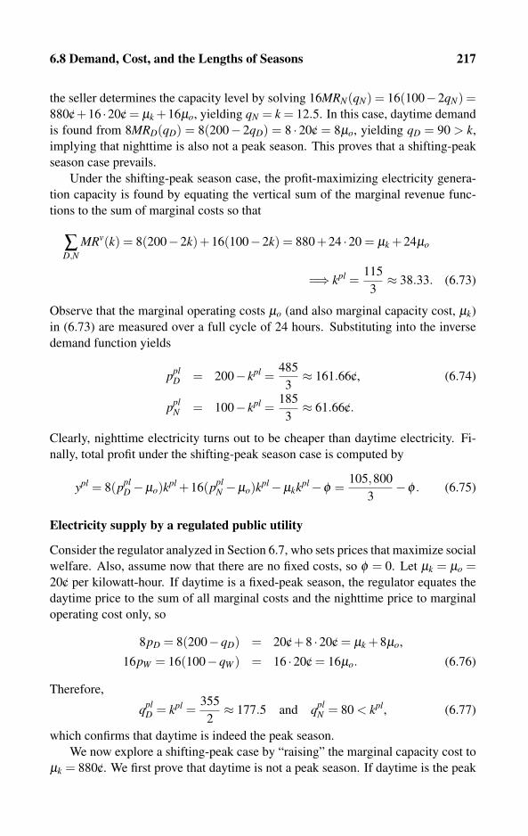
6.8 Demand, Cost, and the Lengths of Seasons 217
the seller determines the capacity level by solving 16MRN(qN) = 16(100−2qN) =880/c+16 ·20/c = μk +16μo, yielding qN = k = 12.5. In this case, daytime demand
is found from 8MRD(qD) = 8(200− 2qD) = 8 · 20/c = 8μo, yielding qD = 90 > k,
implying that nighttime is also not a peak season. This proves that a shifting-peak
season case prevails.
Under the shifting-peak season case, the profit-maximizing electricity genera-
tion capacity is found by equating the vertical sum of the marginal revenue func-
tions to the sum of marginal costs so that
∑D,N
MRv(k) = 8(200−2k)+16(100−2k) = 880+24 ·20 = μk +24μo
=⇒ kpl =115
3≈ 38.33. (6.73)
Observe that the marginal operating costs μo (and also marginal capacity cost, μk)
in (6.73) are measured over a full cycle of 24 hours. Substituting into the inverse
demand function yields
pplD = 200− kpl =
485
3≈ 161.66/c, (6.74)
pplN = 100− kpl =
185
3≈ 61.66/c.
Clearly, nighttime electricity turns out to be cheaper than daytime electricity. Fi-
nally, total profit under the shifting-peak season case is computed by
ypl = 8(pplD−μo)kpl +16(ppl
N −μo)kpl−μkkpl−φ =105,800
3−φ . (6.75)
Electricity supply by a regulated public utility
Consider the regulator analyzed in Section 6.7, who sets prices that maximize social
welfare. Also, assume now that there are no fixed costs, so φ = 0. Let μk = μo =20/c per kilowatt-hour. If daytime is a fixed-peak season, the regulator equates the
daytime price to the sum of all marginal costs and the nighttime price to marginal
operating cost only, so
8pD = 8(200−qD) = 20/c+8 ·20/c = μk +8μo,
16pW = 16(100−qW ) = 16 ·20/c = 16μo. (6.76)
Therefore,
qplD = kpl =
355
2≈ 177.5 and qpl
N = 80 < kpl, (6.77)
which confirms that daytime is indeed the peak season.
We now explore a shifting-peak case by “raising” the marginal capacity cost to
μk = 880/c. We first prove that daytime is not a peak season. If daytime is the peak
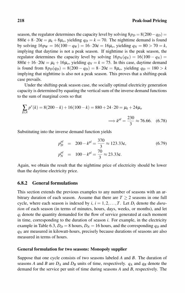
218 Peak-load Pricing
season, the regulator determines the capacity level by solving 8pD = 8(200−qD) =880/c + 8 · 20/c = μk + 8μo, yielding qD = k = 70. The nighttime demand is found
by solving 16pW = 16(100− qW ) = 16 · 20/c = 16μo, yielding qN = 80 > 70 = k,
implying that daytime is not a peak season. If nighttime is the peak season, the
regulator determines the capacity level by solving 16pN(qN) = 16(100− qN) =880/c + 16 · 20/c = μk + 16μo, yielding qN = k = 75. In this case, daytime demand
is found from 8pD(qD) = 8(200− qD) = 8 · 20/c = 8μo, yielding qD = 180 > kimplying that nighttime is also not a peak season. This proves that a shifting-peak
case prevails.
Under the shifting-peak season case, the socially optimal electricity generation
capacity is determined by equating the vertical sum of the inverse demand functions
to the sum of marginal costs so that
∑D,N
pv(k) = 8(200− k)+16(100− k) = 880+24 ·20 = μk +24μo
=⇒ kpl =230
3≈ 76.66. (6.78)
Substituting into the inverse demand function yields
pplD = 200− kpl =
370
3≈ 123.33/c, (6.79)
pplN = 100− kpl =
70
3≈ 23.33/c.
Again, we obtain the result that the nighttime price of electricity should be lower
than the daytime electricity price.
6.8.2 General formulations
This section extends the previous examples to any number of seasons with an ar-
bitrary duration of each season. Assume that there are T ≥ 2 seasons in one full
cycle, where each season is indexed by i, i = 1,2, . . . ,T . Let Di denote the dura-tion of each season (in terms of minutes, hours, days, weeks, or months), and let
qi denote the quantity demanded for the flow of service generated at each moment
in time, corresponding to the duration of season i. For example, in the electricity
example in Table 6.3, DD = 8 hours, DN = 16 hours, and the corresponding qD and
qN are measured in kilowatt-hours, precisely because durations of seasons are also
measured in terms of hours.
General formulation for two seasons: Monopoly supplier
Suppose that one cycle consists of two seasons labeled A and B. The duration of
seasons A and B are DA and DB units of time, respectively. qA and qB denote the
demand for the service per unit of time during seasons A and B, respectively. The

6.8 Demand, Cost, and the Lengths of Seasons 219
prices for the service (per service unit, per unit of time) are denoted by pA and pB.
Linear demand functions are assumed so that pA = αA−βAqA and pB = αB−βBqB,
where αA, αB, βA, and βB are all strictly positive parameters to be estimated by the
econometrician of the firm.
If season A is a peak season, the seller should solve
DAMRA(qA) = DA(αA−2βAqA) = μk +DAμo,
DBMRB(qB) = DB(αB−2βBqB) = DBμo, (6.80)
yielding
kpl = qplA =
DA(αA−μA)−μk
2DAβAand qpl
B =αB−μo
2βB. (6.81)
Clearly, it must be verified at this stage that season A is the peak season by checking
whether qplB ≤ kpl. Otherwise, one should check whether season B might be the
peak season (we do not do it here), or whether a shifting-peak case is encountered.
At this stage, one can also investigate how demand in each season is affected by
extending the duration of the season. More precisely, (6.81) implies that
dkpl
dDA=
dqplA
dDA=
μk
2βAD2A
> 0 anddqpl
BdDA
= 0. (6.82)
Thus, an increase in the duration of the peak season results in a higher investment in
service capacity, and hence in the flow of service provided during the peak season.
In contrast, the off-peak service flow is invariant with respect to changes in the
duration of seasons. This is because at each point in time during the off-peak
season, consumers are charged proportionally to the flow of marginal operating
cost only. In contrast, prolonging the peak season implies that the cost of capacity is
spread over a longer period of time, which permits a higher investment in capacity.
To conclude the general formulation of the two-season analysis for a single
profit-maximizing seller, the prices are computed by
pplA = αA−βAqpl
A =DA(αA + μo)+ μk
2DA,
pplB = αB−βBqpl
B =αB + μo
2. (6.83)
Clearly, dpplA /dDA < 0 implies that the peak-season price drops with an increase in
the duration of the peak season because the cost of capital is spread over a longer
peak season. The off-peak season price does not vary with the duration of the
season because consumers are charged proportionally to the flow of operating cost
only. Finally, the profit level for the case in which season A is the fixed peak is
computed by substituting (6.81) and (6.83) into
ypl = DA(pplA −μo)kpl +DB(ppl
B −μo)qplB −μkkpl−φ . (6.84)
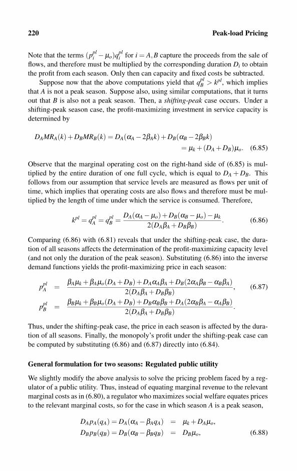
220 Peak-load Pricing
Note that the terms (ppli −μo)q
pli for i = A,B capture the proceeds from the sale of
flows, and therefore must be multiplied by the corresponding duration Di to obtain
the profit from each season. Only then can capacity and fixed costs be subtracted.
Suppose now that the above computations yield that qplB > kpl, which implies
that A is not a peak season. Suppose also, using similar computations, that it turns
out that B is also not a peak season. Then, a shifting-peak case occurs. Under a
shifting-peak season case, the profit-maximizing investment in service capacity is
determined by
DAMRA(k)+DBMRB(k) = DA(αA−2βAk)+DB(αB−2βBk)= μk +(DA +DB)μo. (6.85)
Observe that the marginal operating cost on the right-hand side of (6.85) is mul-
tiplied by the entire duration of one full cycle, which is equal to DA + DB. This
follows from our assumption that service levels are measured as flows per unit of
time, which implies that operating costs are also flows and therefore must be mul-
tiplied by the length of time under which the service is consumed. Therefore,
kpl = qplA = qpl
B =DA(αA−μo)+DB(αB−μo)−μk
2(DAβA +DBβB). (6.86)
Comparing (6.86) with (6.81) reveals that under the shifting-peak case, the dura-
tion of all seasons affects the determination of the profit-maximizing capacity level
(and not only the duration of the peak season). Substituting (6.86) into the inverse
demand functions yields the profit-maximizing price in each season:
pplA =
βAμk +βAμo(DA +DB)+DAαAβA +DB(2αAβB−αBβA)2(DAβA +DBβB)
, (6.87)
pplB =
βBμk +βBμo(DA +DB)+DBαBβB +DA(2αBβA−αAβB)2(DAβA +DBβB)
.
Thus, under the shifting-peak case, the price in each season is affected by the dura-
tion of all seasons. Finally, the monopoly’s profit under the shifting-peak case can
be computed by substituting (6.86) and (6.87) directly into (6.84).
General formulation for two seasons: Regulated public utility
We slightly modify the above analysis to solve the pricing problem faced by a reg-
ulator of a public utility. Thus, instead of equating marginal revenue to the relevant
marginal costs as in (6.80), a regulator who maximizes social welfare equates prices
to the relevant marginal costs, so for the case in which season A is a peak season,
DA pA(qA) = DA(αA−βAqA) = μk +DAμo,
DB pB(qB) = DB(αB−βBqB) = DBμo, (6.88)
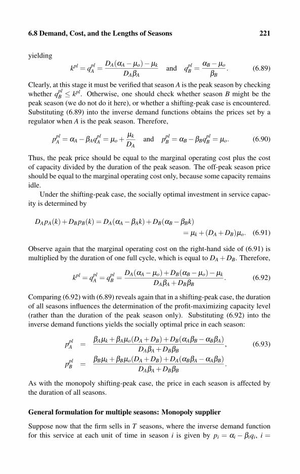
6.8 Demand, Cost, and the Lengths of Seasons 221
yielding
kpl = qplA =
DA(αA−μo)−μk
DAβAand qpl
B =αB−μo
βB. (6.89)
Clearly, at this stage it must be verified that season A is the peak season by checking
whether qplB ≤ kpl. Otherwise, one should check whether season B might be the
peak season (we do not do it here), or whether a shifting-peak case is encountered.
Substituting (6.89) into the inverse demand functions obtains the prices set by a
regulator when A is the peak season. Therefore,
pplA = αA−βAqpl
A = μo +μk
DAand ppl
B = αB−βBqplB = μo. (6.90)
Thus, the peak price should be equal to the marginal operating cost plus the cost
of capacity divided by the duration of the peak season. The off-peak season price
should be equal to the marginal operating cost only, because some capacity remains
idle.
Under the shifting-peak case, the socially optimal investment in service capac-
ity is determined by
DA pA(k)+DB pB(k) = DA(αA−βAk)+DB(αB−βBk)= μk +(DA +DB)μo. (6.91)
Observe again that the marginal operating cost on the right-hand side of (6.91) is
multiplied by the duration of one full cycle, which is equal to DA +DB. Therefore,
kpl = qplA = qpl
B =DA(αA−μo)+DB(αB−μo)−μk
DAβA +DBβB. (6.92)
Comparing (6.92) with (6.89) reveals again that in a shifting-peak case, the duration
of all seasons influences the determination of the profit-maximizing capacity level
(rather than the duration of the peak season only). Substituting (6.92) into the
inverse demand functions yields the socially optimal price in each season:
pplA =
βAμk +βAμo(DA +DB)+DB(αAβB−αBβA)DAβA +DBβB
, (6.93)
pplB =
βBμk +βBμo(DA +DB)+DA(αBβA−αAβB)DAβA +DBβB
.
As with the monopoly shifting-peak case, the price in each season is affected by
the duration of all seasons.
General formulation for multiple seasons: Monopoly supplier
Suppose now that the firm sells in T seasons, where the inverse demand function
for this service at each unit of time in season i is given by pi = αi − βiqi, i =

222 Peak-load Pricing
1,2, . . . ,T . The parameters αi and βi are all strictly positive and are to be estimated
by the econometrician of the firm. The reader is now referred to Section 6.5.2
which describes the general procedure for determining which seasons should be
treated as peak seasons and which are off-peak seasons. This procedure should be
slightly modified to take into account the more general formulation that assumes
that seasons may have different durations. Let Di denote the duration of season i,i = 1,2, . . . ,T .
Once the peak seasons are identified, let the set peak contain all the indexes i,where i is a peak season. The seller then determines the profit-maximizing capacity
level kpl by solving
∑i∈peak
DiMRi(k) = ∑i∈peak
Di(αi−2βik) = μk + μo ∑i∈peak
Di. (6.94)
Observe that the marginal operating cost on the right-hand side of (6.94) is multi-
plied by the sum of the duration of all peak seasons, which is equal to ∑i∈peak Di.
This is because service levels qi are measured as flows.
For each off-peak season i /∈ peak, the seller determines service levels qi by
solving
DiMRi(qi) = Di(αi−2βiqi) = Diμo. (6.95)
The socially optimal prices are then computed by substituting service levels qi into
the inverse demand functions ppli = αi−βiq
pli , where qpl
i = kpl for each i ∈ peak.
Total profit is then computed from
ypl = ∑i∈peak
Di(ppli −μo)kpl + ∑
i/∈peakDi(ppl
i −μo)qpli −μkkpl−φ . (6.96)
General formulation for multiple seasons: Regulated public utility
A regulator who seeks to maximize social welfare equates the vertical sum of de-
mand functions of peak seasons to the sum of marginal and capacity costs. There-
fore, the condition for determining the capacity level kpl (6.94) is now modified
to
∑i∈peak
Di pi(k) = ∑i∈peak
Di(αi−βik) = μk + μo ∑i∈peak
Di. (6.97)
For the off-peak seasons i /∈ peak, (6.95) is now modified to
Di pi(qi) = Di(αi−βiqi) = Diμo. (6.98)
Prices are then computed by substituting service levels qi into the inverse demand
functions ppli = αi−βiq
pli , where qpl
i = kpl for each i ∈ peak.
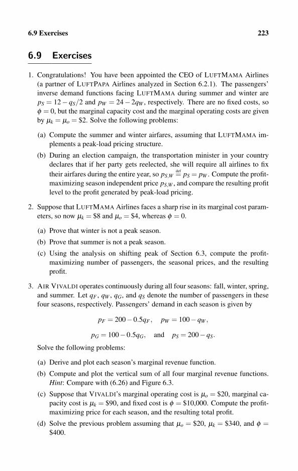
6.9 Exercises 223
6.9 Exercises
1. Congratulations! You have been appointed the CEO of LUFTMAMA Airlines
(a partner of LUFTPAPA Airlines analyzed in Section 6.2.1). The passengers’
inverse demand functions facing LUFTMAMA during summer and winter are
pS = 12− qS/2 and pW = 24− 2qW , respectively. There are no fixed costs, so
φ = 0, but the marginal capacity cost and the marginal operating costs are given
by μk = μo = $2. Solve the following problems:
(a) Compute the summer and winter airfares, assuming that LUFTMAMA im-
plements a peak-load pricing structure.
(b) During an election campaign, the transportation minister in your country
declares that if her party gets reelected, she will require all airlines to fix
their airfares during the entire year, so pS,Wdef= pS = pW . Compute the profit-
maximizing season independent price pS,W , and compare the resulting profit
level to the profit generated by peak-load pricing.
2. Suppose that LUFTMAMA Airlines faces a sharp rise in its marginal cost param-
eters, so now μk = $8 and μo = $4, whereas φ = 0.
(a) Prove that winter is not a peak season.
(b) Prove that summer is not a peak season.
(c) Using the analysis on shifting peak of Section 6.3, compute the profit-
maximizing number of passengers, the seasonal prices, and the resulting
profit.
3. AIR VIVALDI operates continuously during all four seasons: fall, winter, spring,
and summer. Let qF , qW , qG, and qS denote the number of passengers in these
four seasons, respectively. Passengers’ demand in each season is given by
pF = 200−0.5qF , pW = 100−qW ,
pG = 100−0.5qG, and pS = 200−qS.
Solve the following problems:
(a) Derive and plot each season’s marginal revenue function.
(b) Compute and plot the vertical sum of all four marginal revenue functions.
Hint: Compare with (6.26) and Figure 6.3.
(c) Suppose that VIVALDI’s marginal operating cost is μo = $20, marginal ca-
pacity cost is μk = $90, and fixed cost is φ = $10,000. Compute the profit-
maximizing price for each season, and the resulting total profit.
(d) Solve the previous problem assuming that μo = $20, μk = $340, and φ =$400.

224 Peak-load Pricing
4. The TWOSEASONS Hotel operates continuously during summer and winter. Let
qS and qW denote the summer and winter number of vacationers, respectively.
The inverse demand function is pS = 120− 2qS− qW during the summer, and
pW = 120−3qW −qS during the winter. Solve the following problems using the
analysis of interdependent demand in Section 6.6.
(a) Write down the summer and winter total revenue functions, and derive the
corresponding four marginal revenue functions.
(b) Suppose now that the hotel’s fixed cost is φ = $1000 and marginal capacity
and operating costs are μk = μo = $20. Using the analysis of interdepen-
dent demand given in Section 6.6, compute the hotel’s profit-maximizing
summer and winter rates and the resulting total profit.
(c) Solve the previous problem assuming that the hotel’s cost parameters are
now given by φ = $500, μk = $40, and μo = $20.
5. Suppose that LUFTMAMA Airlines, described in Exercise 1, has been national-
ized and is now being operated as a regulated public utility. Using the analysis
of Section 6.7, compute the socially optimal summer and winter airfares as well
as the socially optimal seating capacity.
6. Suppose that the company described in Exercise 2 has been nationalized and is
now being operated as a regulated public utility. Compute the socially optimal
summer and winter airfares as well as the socially optimal seating capacity.
7. Suppose that AIR VIVALDI, described in Exercise 3, has been nationalized and
is now being operated as a regulated public utility. Compute the socially optimal
airfare in each season, as well as the socially optimal seating capacity assuming
that μo = $20, μk = $100, and there are no fixed costs, φ = 0.
8. As the new manager of the four-star SCHLAFEN Hotel, you are in charge of
setting room rates during the summer season, denoted by pS, and during the
winter season, denoted by pW . The duration of the summer and winter seasons,
also described in Table 6.3, are DS = 120 days and DW = 245 days, respectively.
The marginal capacity cost (infrastructure cost of adding one additional room
per one year) is μk = $24,000. The marginal operating cost (cost of cleaning up
a room after it has been occupied for one night) is μo = $20. Finally, the inverse
demand functions for rooms are given by
pS = 240− qS
2and pW = 240−qW ,
where qS and qW are the number of rooms demanded during each summer night
and each winter night, respectively. Solve the following problems:
6.9 Exercises 225
(a) Compute the most profitable room rates during summer nights and winter
nights, the investment in room capacity, and the resulting profit level, as-
suming that the SCHLAFEN Hotel is the only hotel in a 200-mile radius.
(b) Compute the socially optimal room rates during summer and winter nights
and the investment in room capacity assuming the hotel is now operated as
a regulated public utility.

Chapter 7
Advance Booking
7.1 Two Booking Periods with Two Service Classes 2327.1.1 A numerical example
7.1.2 General formulation
7.1.3 Salvage value of capacity
7.1.4 Dynamic advance booking for a small population
7.2 Multiple Periods with Two Service Classes 2387.2.1 Single capacity unit: Example I
7.2.2 Single capacity unit: Example II
7.2.3 Two capacity units example
7.2.4 Large-capacity example
7.3 Multiple Booking Periods and Service Classes 2457.3.1 General formulation
7.3.2 Computer algorithm
7.4 Dynamic Booking with Marginal Operating Cost 2487.4.1 Converting prices to marginal profits
7.4.2 Computer algorithm
7.5 Network-based Dynamic Advance Booking 2507.5.1 A numerical example
7.5.2 General formulation
7.6 Fixed Class Allocations 2547.6.1 Nonoptimality of fixed class allocations
7.6.2 How to determine fixed class allocations: An example
7.6.3 Computer algorithm for fixed class allocations
7.7 Nested Class Allocations 2587.7.1 Nested class allocation versus fixed allocations
7.7.2 How to determine nested class allocations: An example
7.7.3 Computer algorithm for nested class allocations
7.7.4 Protective (theft) nested capacity allocations
7.8 Exercises 262
228 Advance Booking
Service providers, particularly providers of services related to travel, engage in
advance booking that use a wide variety of advance reservation systems. From
consumers’ perspective, this practice seems to be beneficial for the following two
reasons:
• Value of time and capacity constraint: Advance reservations save considerable
amount of time for consumers as otherwise they would have to travel several
times to the theater, airport, train station, or hotel, just to find out that these
services may have already been fully booked.
• Purchase of complementary services: Travel arrangements almost always consist
of a wide variety of complementary services that must be booked from multiple
providers (flights, trains, hotels). In addition, travelers must alter their work
schedule, which may include asking for vacation time or a leave of absence.
Advance reservations ensure the fulfilment of these multiple obligations at the
same time.
Whereas both of the above examples demonstrate why advance booking is ben-
eficial to consumers, the purpose of this chapter is to show that advance booking
also enhances the profit of service providers. Moreover, this chapter suggests sev-
eral algorithms under which advance booking becomes the major strategic tool
for making YM most profitable. Perhaps the most interesting feature of advance
reservation systems is that they can be used to identify and sort consumers accord-
ing to their willingness to pay without having to formally ask them to reveal their
preferences. For example, students who can plan their vacation time according to
semester schedules posted by their schools tend to purchase discounted advance-
purchase tickets. In contrast, people who travel on business generally cannot plan
their business trips in advance and therefore resort to last-minute full-price tickets.
In the language of economics, well-designed advance booking mechanisms induce
consumers to reveal their preferences and their true types by simply observing what
type of service classes they book.
The formal analysis in this chapter is presented according to an increasing or-
der of complexity associated with the number of booking periods, the number of
booking classes (fare classes), and the amount of capacity. This is because profit-
maximizing YM requires the use of dynamic optimization, commonly referred to as
dynamic programming. The two booking period cases are analyzed in great detail
to enable readers to gain the full intuition behind the dynamics of booking strate-
gies. Readers who wish to avoid the entire dynamic programming analysis should
skip Sections 7.1 through 7.5 and concentrate on Sections 7.6 and 7.7 only.
The analysis in this chapter assumes that time is discrete and is indexed by
t = 1,2, . . . ,T,T + 1. Potential consumers are allowed to book during the periods
t = 1, . . . ,T . Then, the contracted service is delivered in period T +1 when no fur-
ther bookings can be made. The service provider announces a number of booking
Advance Booking 229
classes indexed by i, i ∈B = {A,B,C, . . .}, and the price for each booking class
(fare class) as PA, PB, PC, and so on, where PA > PB > PC > .. . . Thus, class A is
the most expensive class, followed by class B, and so on. Lastly, let P0 = 0 denote
a zero revenue “obtained” from a consumer who does not make a reservation. That
is, for analytical convenience we treat a period when no booking is made as if a
consumer requests to be booked at a class for which she has to pay P0 = 0 for the
service. Because prices are written in capital letters, they are treated as exogenous
parameters of the model developed in this chapter (compare P in Table 1.4 with pin Table 1.5).
We denote by K the amount of service capacity, which equals the maximum
possible total number of bookings that can be made in all classes combined. Hence,
by the end of period T , the total number of bookings cannot exceed K.
The potential consumer population consists of a fraction, denoted by πA, of
high-valuation consumers who are willing to pay PA for a class A service, where
0≤ πA ≤ 1. Similarly, πB, πC, and so on are the fractions of the population willing
to pay for class B and class C services, respectively. Lastly, we assume that some
part of the population will either not use the reservation system or will not book
after contacting the reservation agent. We denote this fraction by π0. Formally,
we define π0 = 1−∑i∈B π i as the fraction of the population who never books this
service.
Most of our formal analysis also interprets the fraction π i as the probabilitythat a booking on a certain class will be made. For this interpretation to be valid,
we need to distinguish between two types of potential consumer populations as
described in the following definition:
DEFINITION 7.1
We say that the potential consumer population is
• Large if the fractions π i are also the probabilities that a consumer will request
a booking on class i ∈ B, and that these probabilities are independent of the
number of bookings that have been made before this booking request.
• Small if the fractions π i, i ∈B, reflect initial probabilities; however, they must
be updated after each booking period to reflect how many bookings of each con-
sumer type have already been made.
Thus, for a large population, the expected composition of the consumer population
remains unchanged during all booking periods and is independent of the number
and type of bookings already made. This is not the case for a small population
size, for which if many bookings are made for class B, the service provider should
expect future bookings to consist of all classes other than class B. In this case, the
probability of a consumer requesting a booking on a certain class must be updated
after each booking period. Unless stated otherwise, the analysis in this book will
be restricted as follows:
230 Advance Booking
ASSUMPTION 7.1
The potential consumer population is large according to Definition 7.1(a).
The reader is referred to Subsection 7.1.4 where our analysis deviates from this
assumption.
Before we begin describing the algorithms behind profitable advance booking
systems, we must specify the timing under which reservations are made. We make
the following assumption:
ASSUMPTION 7.2
In each period t, t = 1,2, . . . ,T , there is at most one consumer who books the
service.
Assumption 7.2 is motivated by the fact that a computer system can book at most
one person at a time, because before allowing any further reservations to be made,
the software must readjust the level of remaining capacity. There are two additional
ways to justify the use of this assumption. First, we can assume that time periods
are very short. In fact, our T -period dynamic model can easily accommodate short
time periods corresponding to a large number of booking periods (higher levels of
T ). Second, time periods can be adjusted during the 24-hour cycle so that off-peak
periods (say, late night) will be made relatively long whereas peak periods will be
made very short.
Clearly, if K ≥ T , the capacity constraint is not binding and the service provider
should accept any booking request. Accordingly, we make the following assump-
tion:
ASSUMPTION 7.3
(a) The total amount of capacity available for booking is smaller than the number
of booking periods. Formally, K < T .
(b) Overbooking is not allowed.
(c) Capacity can be costlessly and instantaneously shifted among the various ser-
vice classes.
Assumption 7.3(a) makes our problem interesting, as it eliminates the trivial case
of excess capacity in which every booking request should be accommodated. As-
sumption 7.3(b) imposes a restriction on our analysis. Because overbooking is
widely observed and is considered an integral part of YM, we devote an entire
chapter to the entire analysis of overbooking, which is given in Chapter 9.
Assumption 7.3(c) implies that classes differ mainly according to the amount of
extra services given to the customers, or by the restriction levels imposed on their
tickets. In some services, however, reallocation of capacity among the different
booking classes is costly and time consuming. For example, aircraft seats assigned
to first-class passengers are much wider than the seats assigned to economy-class
passengers. In this case, a reallocation of aircraft capacity is both costly and time
Advance Booking 231
consuming and therefore cannot adhere to an otherwise profit-maximizing book-
ing strategy. In this situation, only fixed class allocations of capacity are possible,
which we analyze in Section 7.6. However, in many instances, even physical capac-
ity can be easily shifted from one class to another. For example, a railway company
may replace a regular car with a more luxurious first-class car (or even a sleeper)
when it observes a high demand for its first-class tickets. For this reason, most of
our analysis will rely on Assumption 7.3(c).
Given that at most one consumer can be booked in each period t, let Pt ∈{P0,PA,PB, . . .} denote the price/fare for the booking class requested by a period tconsumer. The reader is reminded that P0 = 0 denotes the (non)revenue from a
nonbooking consumer. Also, let dt denote the decision rule for whether or not to
accommodate a booking request by a period t consumer. This decision can be au-
tomated by a computerized reservation system. dt = 1 means that the reservation
has been confirmed and one unit of capacity is reserved for the period t booking
consumer. In contrast, dt = 0 means that the period t booking request has been
denied. Altogether, the period t profit can be written as dt(Pt − μo), where μo
is the marginal operating cost of providing an additional unit of service (or the
marginal cost of making an additional successful booking). Finally, we assume
that the marginal operating cost is zero (μo = 0). This assumption is relaxed in
Section 7.4, which demonstrates how our basic models can be easily modified to
capture marginal profits associated with having strictly positive marginal operating
cost.
The earliest condition for accepting or denying a consumer’s booking request is
attributed to Littlewood (1972). Other scientific literature on the theory of dynamic
booking systems includes Lee and Hersh (1993) and Lautenbacher and Stidham
(1999); see also Talluri and van Ryzin (2004, Ch. 2). Most of the analysis in this
chapter uses dynamic programming. Our main purpose is to develop the logic
behind the algorithm for deciding whether and what type of booking offers should
be accepted by the service provider in each booking period t = 1,2, . . . ,T . The
solution method we use in this book is called Bellman’s principle of optimalitydue to Bellman (1957). In general, the key to solving any finite-horizon dynamic
optimization is to work the solution backward using backward induction. That is,
we start with the last period t = T and work backward period by period until the
first booking period t = 1. Our analysis in each period t is divided into two parts:
• Booking decision: In each booking period t, we determine a decision rule
dt(Pt) ∈ {0,1}, which indicates whether to reject or accept a booking request
for the class associated with the price Pt ∈ {PA,PB, . . .}. The period t decision
rule is determined by maximizing the sum of current profit associated with the
requested Pt , and all future value of remaining capacity kt+1.
232 Advance Booking
• Expected value of capacity: Given the optimal period t decision rule dt(Pt), we
compute the expected value of period t available capacity, which we denote by
EV (kt).
That is, each booking decision must take into account that accepting a booking in
period t will reduce the amount of capacity available for booking in period t + 1.
Formally, if a booking is accepted, the capacity available for bookings in periods t +1 and on becomes kt+1 = kt − 1. In contrast, if a booking is not made or simply
denied, the amount of capacity available for booking during period t + 1 and on
remains the same level given by kt+1 = kt . Thus, the trade-off between accepting
a current booking request and the effects of a reduction in the amount of capacity
available for booking in subsequent periods is evaluated by comparing the period tprice offer with the difference between the expected period t +1 value of capacity
resulting from a reduction in one unit of capacity. This difference is given by
EV (kt)−EV (kt −1) if dt(Pt) = 1.
7.1 Two Booking Periods with Two Service Classes
Let t = 1,2,3 denote two booking periods ending with period t = 3 when the service
is scheduled to be delivered. Let there be two booking classes labeled class A and
class B. The service provider announces the prices for these classes as PA and
PB, where PA > PB > 0. The probabilities of booking a consumer in class A and
class B in a given period are given by πA and πB, respectively, where 0 ≤ π i < 1.
The probability of not booking any consumer in a given period is π0 = 1−πA−πB. To close the model, and for the sake of this demonstration only, we assume
that the capacity is limited to a single consumer only so that only one booking
can be made. Formally, we set K = 1. Subsection 7.1.1 starts with a numerical
example. Subsection 7.1.2 follows with more formal and general presentations.
Subsection 7.1.3 introduces salvage value of capacity into the model.
7.1.1 A numerical example
Suppose that the first-class price is PA = $40, whereas second class is offered for
PB = $10. The corresponding probabilities of booking a consumer into the two
classes in each given period are πA = 0.1 and πB = 0.8. This means that the proba-
bility that no booking is made in a given period is π0 = 0.1. Table 7.1 summarizes
the data on the potential consumer population.
Because period t = 2 is the last booking period, any booking request should
be accepted provided that at least one unit of capacity is available. Otherwise,
some capacity will remain unused in period 3 when the service is scheduled to be
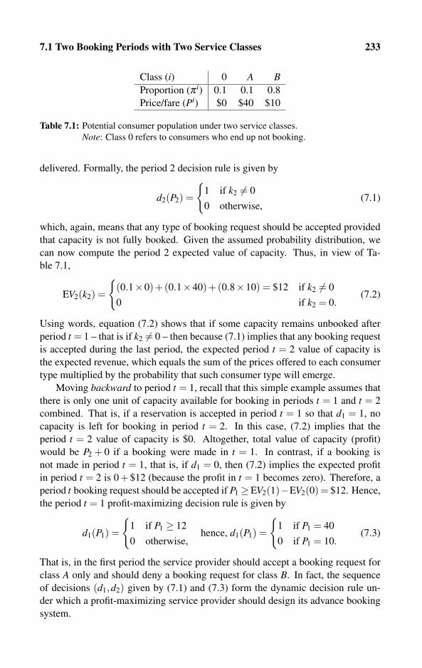
7.1 Two Booking Periods with Two Service Classes 233
Class (i) 0 A BProportion (π i) 0.1 0.1 0.8
Price/fare (Pi) $0 $40 $10
Table 7.1: Potential consumer population under two service classes.
Note: Class 0 refers to consumers who end up not booking.
delivered. Formally, the period 2 decision rule is given by
d2(P2) =
{1 if k2 �= 0
0 otherwise,(7.1)
which, again, means that any type of booking request should be accepted provided
that capacity is not fully booked. Given the assumed probability distribution, we
can now compute the period 2 expected value of capacity. Thus, in view of Ta-
ble 7.1,
EV2(k2) =
{(0.1×0)+(0.1×40)+(0.8×10) = $12 if k2 �= 0
0 if k2 = 0.(7.2)
Using words, equation (7.2) shows that if some capacity remains unbooked after
period t = 1 – that is if k2 �= 0 – then because (7.1) implies that any booking request
is accepted during the last period, the expected period t = 2 value of capacity is
the expected revenue, which equals the sum of the prices offered to each consumer
type multiplied by the probability that such consumer type will emerge.
Moving backward to period t = 1, recall that this simple example assumes that
there is only one unit of capacity available for booking in periods t = 1 and t = 2
combined. That is, if a reservation is accepted in period t = 1 so that d1 = 1, no
capacity is left for booking in period t = 2. In this case, (7.2) implies that the
period t = 2 value of capacity is $0. Altogether, total value of capacity (profit)
would be P2 + 0 if a booking were made in t = 1. In contrast, if a booking is
not made in period t = 1, that is, if d1 = 0, then (7.2) implies the expected profit
in period t = 2 is 0 + $12 (because the profit in t = 1 becomes zero). Therefore, a
period t booking request should be accepted if P1≥EV2(1)−EV2(0) = $12. Hence,
the period t = 1 profit-maximizing decision rule is given by
d1(P1) =
{1 if P1 ≥ 12
0 otherwise,hence, d1(P1) =
{1 if P1 = 40
0 if P1 = 10.(7.3)
That is, in the first period the service provider should accept a booking request for
class A only and should deny a booking request for class B. In fact, the sequence
of decisions (d1,d2) given by (7.1) and (7.3) form the dynamic decision rule un-
der which a profit-maximizing service provider should design its advance booking
system.

234 Advance Booking
Let us now compute the profit for some possible realizations of booking re-
quests. Suppose that in period 1 a consumer requests a class B booking, meaning
that P1 = $10, whereas another consumer requests a class B booking in period 2.
The decision rule (7.3) implies that d1($10) = 0 (booking request denied), whereas
d2($10) = 1 (accepted). Hence, total realized profit is y = $10.
Perhaps the most interesting feature of this example is that the dynamic de-
cision rule (d1,d2) that we found may profitably lead to a sequence of events in
which capacity that could have been booked remains unused. This happens when a
consumer who wishes to be booked into class B in period t = 1 is denied booking
and when eventually no one is booked in period t = 2 as well. Formally, consider
the sequence of booking requests given by P1 = $10 and P2 = $0. This sequence of
events is realized with probability πB×π0 = 0.8×0.1 = 0.08, which is the proba-
bility that a class B booking request is made (and denied) in period t = 1 and that no
booking is made in period t = 1. Because d1($10) = 0 and d2($0) = 0, the realized
profit is y = $0.
Finally, it may be interesting to compute the period t = 1 value of capacity
since the value provides the key indication as to whether investing in this capacity
is profitable for this service provider. The decision rule given in (7.3) and Table 7.1
implies that
EV1(1) = 0.1(40+0)+0.9(0+12) = $14.8. (7.4)
Equation (7.4) reflects the maximum amount of money the service provider may
want to spend on buying or renting a single unit of capacity.
7.1.2 General formulation
Although specific examples are extremely helpful in demonstrating the logic behind
dynamic booking strategies, they often fail to demonstrate some general rules that
govern dynamic optimizations. More precisely, general formulations have some
advantages over specific examples in that they can condense the optimization rules
into a small number of equations that apply to every booking period t. In contrast,
analyzing specific examples requires the characterization of T separate equations
corresponding to each booking period.
We now formalize our simple two-booking period problem. Using general no-
tation, the booking periods are now labeled T −1 and T (which is the last booking
period). The service is then delivered in period T + 1. Applying Bellman’s prin-
ciple of optimality to the present problem means that at each point of time t, the
seller must choose a booking strategy to maximize the sum of expected value of
capacity from period t (inclusive) until period T . The expected sum of future value
of capacity is influenced by how much capacity is available for booking in future
periods.
Starting with the last booking period, the seller chooses to book (dT = 1) or
to deny booking (dT = 0), yielding the profit (revenue in this case) given by dT PT ,
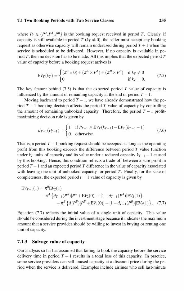
7.1 Two Booking Periods with Two Service Classes 235
where PT ∈ {P0,PA,PB} is the booking request received in period T . Clearly, if
capacity is still available in period T (kT �= 0), the seller must accept any booking
request as otherwise capacity will remain underused during period T +1 when the
service is scheduled to be delivered. However, if no capacity is available in pe-
riod T , then no decision has to be made. All this implies that the expected period Tvalue of capacity before a booking request arrives is
EVT (kT ) =
{(π0×0)+(πA×PA)+(πB×PB) if kT �= 0
0 if kT = 0.(7.5)
The key feature behind (7.5) is that the expected period T value of capacity is
influenced by the amount of remaining capacity at the end of period T −1.
Moving backward to period T −1, we have already demonstrated how the pe-
riod T − 1 booking decision affects the period T value of capacity by controlling
the amount of remaining unbooked capacity. Therefore, the period T − 1 profit-
maximizing decision rule is given by
dT−1(PT−1) =
{1 if PT−1 ≥ EVT (kT−1)−EVT (kT−1−1)0 otherwise.
(7.6)
That is, a period T −1 booking request should be accepted as long as the operating
profit from this booking exceeds the difference between period T value function
under kT units of capacity and its value under a reduced capacity kT−1−1 caused
by this booking. Hence, this condition reflects a trade-off between a sure profit in
period T−1 and an expected period T difference in the value of capacity associated
with leaving one unit of unbooked capacity for period T . Finally, for the sake of
completeness, the expected period t = 1 value of capacity is given by
EVT−1(1) = π0EV2(1)
+πA{dT−1(PA)[PA +EV2(0)]+ [1−dT−1(PA)]EV2(1)}
+πB{d(PB)[PB +EV2(0)]+ [1−dT−1(PB)]EV2(1)}
. (7.7)
Equation (7.7) reflects the initial value of a single unit of capacity. This value
should be considered during the investment stage because it indicates the maximum
amount that a service provider should be willing to invest in buying or renting one
unit of capacity.
7.1.3 Salvage value of capacity
Our analysis so far has assumed that failing to book the capacity before the service
delivery time in period T + 1 results in a total loss of this capacity. In practice,
some service providers can sell unused capacity at a discount price during the pe-
riod when the service is delivered. Examples include airlines who sell last-minute
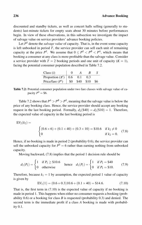
236 Advance Booking
discounted and standby tickets, as well as concert halls selling (generally to stu-
dents) last-minute tickets for empty seats about 30 minutes before performances
begin. In view of these observations, in this subsection we investigate the impact
of salvage value on service providers’ advance booking policies.
Let PS denote the salvage value of capacity. That is, in the event some capacity
is left unbooked in period T , the service provider can sell each unit of remaining
capacity at the price PS. We assume that 0 ≤ PS < PB < PA, which means that
booking a consumer at any class is more profitable than the salvage value. Consider
a service provider with T = 2 booking periods and one unit of capacity (K = 1),
facing the potential consumer population described in Table 7.2.
Class (i) 0 A B SProportion (π i) 0.6 0.1 0.3
Price/fare (Pi) $0 $40 $10 $6
Table 7.2: Potential consumer population under two fare classes with salvage value of ca-
pacity PS = $6.
Table 7.2 shows that PA > PB > PS, meaning that the salvage value is below the
price of any booking class. Hence, the service provider should accept any booking
request in the last booking period. Formally, d2($40) = d2($10) = 1. Therefore,
the expected value of capacity in the last booking period is
EV2(k2) = {(0.6×6)+(0.1×40)+(0.3×10) = $10.6 if k2 �= 0
0 if k2 = 0.(7.8)
Hence, if no booking is made in period 2 (probability 0.6), the service provider can
sell the unbooked capacity for PS = 6 rather than earning nothing from unbooked
capacity.
Moving backward, (7.8) implies that the period 1 decision rule should be
d1(P1) =
{1 if P1 ≥ $10.6
0 otherwisehence d1(P1) =
{1 if P1 = $40
0 if P1 = $10.(7.9)
Therefore, because k1 = 1 by assumption, the expected period 1 value of capacity
is given by
EV1(1) = (0.6+0.3)10.6+(0.1×40) = $14.6. (7.10)
That is, the first term in (7.10) is the expected value of capacity if no booking is
made in period 1. This happens when either no consumer requests a booking (prob-
ability 0.6) or a booking for class B is requested (probability 0.3) and denied. The
second term is the immediate profit if a class A booking is made with probabil-
ity 0.1.

7.1 Two Booking Periods with Two Service Classes 237
Finally, we now ask, What is the effect of having a strictly positive salvage
value on the decision regarding which booking requests to accept? To answer this
question, let us assume that capacity does not have any salvage value, so PS = 0.
Then, (7.8) becomes EV2(P2,k2) = (0.6× $0) + (0.1× $40) + (0.3× $10) = $7
provided that k2 �= 0. Because now EV2(P2,k2) < $10, the period 1 decision rule
(7.9) now changes to d1($40) = 1 as well as d1($10) = 1. That is, now that capacity
does not have any salvage value, the profit-maximizing decision rule in any period
is to accept all booking requests, including a booking request for the less profitable
class B.
7.1.4 Dynamic advance booking for a small population
This subsection demonstrates how our analysis could be modified to capture a small
consumer population, as described by Definition 7.1. When the consumer popula-
tion is small, the service provider must revise the probability of realizing requests
for each booking class by subtracting the consumers who have already been booked
from the list of potential customers and the list of potential requests for the booked
classes.
Table 7.3 displays a simple example with two service classes, A and B; two
booking periods, t = 1,2; one unit of capacity, K = 1; and five potential consumers.
These five consumers are divided as follows: One consumer is expected not to make
any booking (P0 = 0), one consumer is expected to request a booking on class A(PA = $40), and the remaining three are expected to request class B (P0 = $10).
The resulting period t = 1 probabilities of booking on each class i are listed as π i1
in Table 7.3.
Class (i) 0 A B EV2(1)Price (Pi) $0 $40 $10
π i1
15
15
35
π i2 (given P1 = $0) 0 1
434
1440+ 3
410 = $17.5
π i2 (given P1 = $40) 1
40 3
4140+ 3
410 = $7.5
π i2 (given P1 = $10) 1
414
12
1440+ 1
210 = $15
Table 7.3: Small consumer population: Illustration for five consumers.
The important thing to notice in Table 7.3 is that when the population is small,
the probability of booking on each class during period t = 2 depends on what type
of consumer makes a request in period t = 1. Recall that under a large consumer
population (assumed throughout this chapter), the probability of booking on each
class remains constant during the entire booking process. Here, if no booking is
made in period t = 1, it means that in period t = 2 the service provider knows
for certain that either class A or B will be requested. If class A is requested in

238 Advance Booking
period t = 1, the service provider knows for certain that class A will be requested
in period t = 2, hence the initial probability πA1 = 1/5 drops to πA
2 = 0. Similarly, if
class B is requested in t = 1, the number of potential consumers requesting class Bfalls from three to two. Hence, πB
1 = 3/5 drops to πB2 = 1/2.
Once period t = 2 expected values of capacity are computed, we can proceed to
our main investigation, which is characterizing the decision rules regarding which
booking requests to accept during the two booking periods, d1(P1) and d2(P2). The
logic behind the construction of these decision rules is identical to that given in all
previous sections. More precisely, working backward from period t = 2, clearly
d2($40) = d2($10) = 1 as otherwise capacity will remain unused during the period
when the service is scheduled to be delivered.
Moving backward to period t = 1, the generalized decision rule given by (7.6)
implies that a booking request for class A should be accepted because P1 = $40 ≥EV2(1)− EV2(0) = $7.5. Similarly, a period t = 1 booking request for class Bshould be denied because P1 = $10 < EV2(1)−EV2(0) = $15. Therefore,
d1(P1) =
{1 if P1 = $40
0 otherwise,and d2(P2) =
{1 if P2 = $40
1 if P2 = $10.(7.11)
7.2 Multiple Periods with Two Service Classes
So far, our analysis has been restricted to T = 2 booking periods. In this section,
we extend the model to any number of booking periods, thus allowing for T > 2.
Subsection 7.2.1 extends the single-unit capacity example of Subsection 7.1.1. Sub-
section 7.2.3 analyzes K = 2 units of capacity. Finally, Subsection 7.2.4 provides
the general formulation for any number of T booking periods, and any level of
capacity K.
7.2.1 Single capacity unit: Example I
We now extend the two booking examples analyzed in Subsection 7.1.1 to any
number of booking periods indexed by t = 1,2, . . . ,T . Recalling (7.2), the expected
value of capacity in the last booking period is
EVT (kT ) =
{(0.1×0)+(0.1×40)+(0.8×10) = $12 if kT �= 0
0 if kT = 0.(7.12)
Moving backward to period T − 1, recall that the decision rule (7.3) implies
that the service provider should accept a booking request PT−1 = PA = $40 so that
dT−1($40) = 1, and deny a booking request PT−1 = PB = $10 so that dT−1($10) =
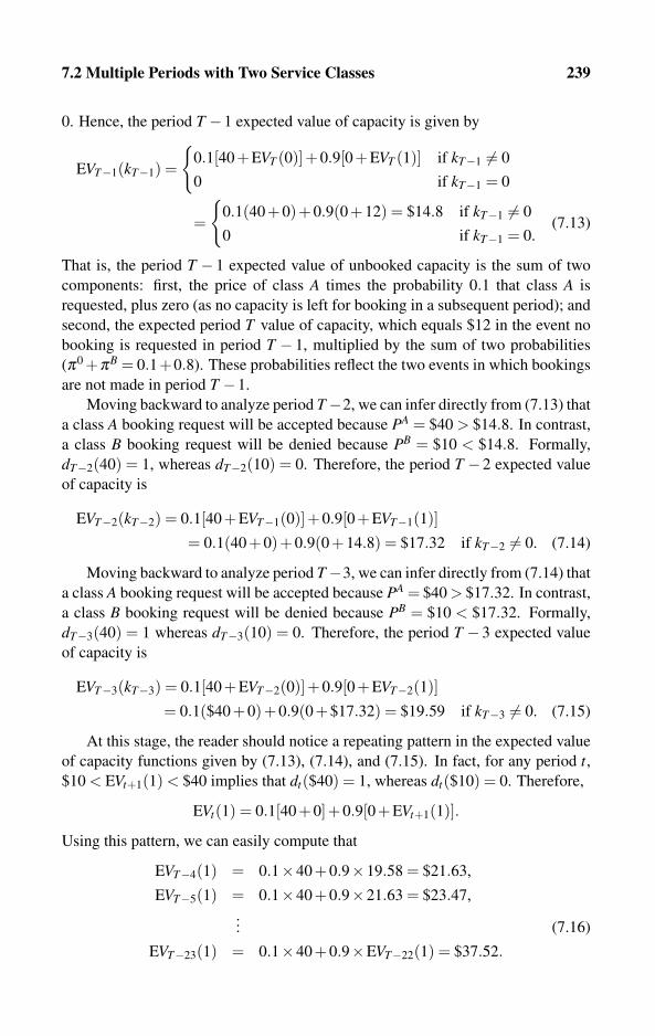
7.2 Multiple Periods with Two Service Classes 239
0. Hence, the period T −1 expected value of capacity is given by
EVT−1(kT−1) =
{0.1[40+EVT (0)]+0.9[0+EVT (1)] if kT−1 �= 0
0 if kT−1 = 0
=
{0.1(40+0)+0.9(0+12) = $14.8 if kT−1 �= 0
0 if kT−1 = 0.(7.13)
That is, the period T − 1 expected value of unbooked capacity is the sum of two
components: first, the price of class A times the probability 0.1 that class A is
requested, plus zero (as no capacity is left for booking in a subsequent period); and
second, the expected period T value of capacity, which equals $12 in the event no
booking is requested in period T − 1, multiplied by the sum of two probabilities
(π0 +πB = 0.1+0.8). These probabilities reflect the two events in which bookings
are not made in period T −1.
Moving backward to analyze period T−2, we can infer directly from (7.13) that
a class A booking request will be accepted because PA = $40 > $14.8. In contrast,
a class B booking request will be denied because PB = $10 < $14.8. Formally,
dT−2(40) = 1, whereas dT−2(10) = 0. Therefore, the period T −2 expected value
of capacity is
EVT−2(kT−2) = 0.1[40+EVT−1(0)]+0.9[0+EVT−1(1)]= 0.1(40+0)+0.9(0+14.8) = $17.32 if kT−2 �= 0. (7.14)
Moving backward to analyze period T−3, we can infer directly from (7.14) that
a class A booking request will be accepted because PA = $40 > $17.32. In contrast,
a class B booking request will be denied because PB = $10 < $17.32. Formally,
dT−3(40) = 1 whereas dT−3(10) = 0. Therefore, the period T − 3 expected value
of capacity is
EVT−3(kT−3) = 0.1[40+EVT−2(0)]+0.9[0+EVT−2(1)]= 0.1($40+0)+0.9(0+$17.32) = $19.59 if kT−3 �= 0. (7.15)
At this stage, the reader should notice a repeating pattern in the expected value
of capacity functions given by (7.13), (7.14), and (7.15). In fact, for any period t,$10 < EVt+1(1) < $40 implies that dt($40) = 1, whereas dt($10) = 0. Therefore,
EVt(1) = 0.1[40+0]+0.9[0+EVt+1(1)].
Using this pattern, we can easily compute that
EVT−4(1) = 0.1×40+0.9×19.58 = $21.63,
EVT−5(1) = 0.1×40+0.9×21.63 = $23.47,
... (7.16)
EVT−23(1) = 0.1×40+0.9×EVT−22(1) = $37.52.
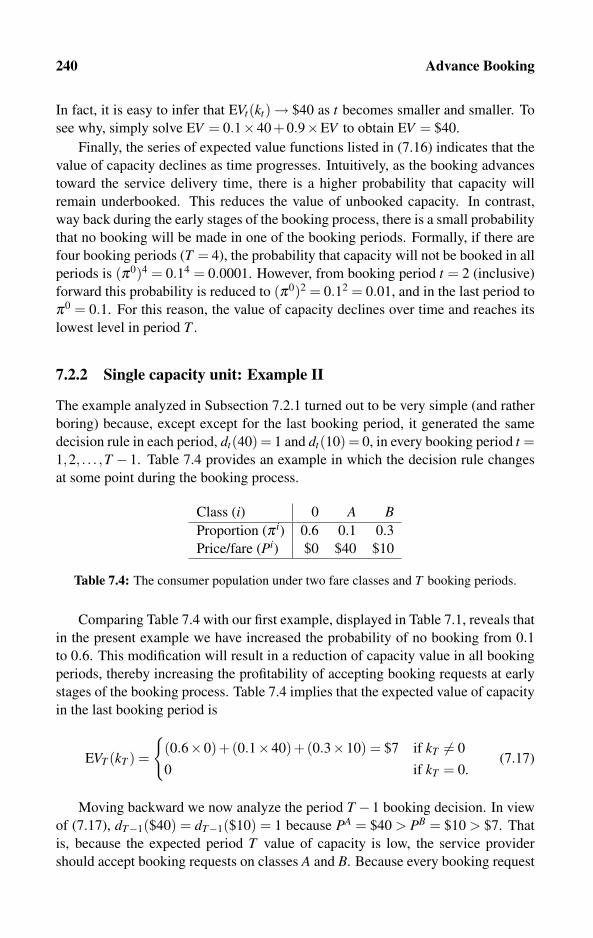
240 Advance Booking
In fact, it is easy to infer that EVt(kt)→ $40 as t becomes smaller and smaller. To
see why, simply solve EV = 0.1×40+0.9×EV to obtain EV = $40.
Finally, the series of expected value functions listed in (7.16) indicates that the
value of capacity declines as time progresses. Intuitively, as the booking advances
toward the service delivery time, there is a higher probability that capacity will
remain underbooked. This reduces the value of unbooked capacity. In contrast,
way back during the early stages of the booking process, there is a small probability
that no booking will be made in one of the booking periods. Formally, if there are
four booking periods (T = 4), the probability that capacity will not be booked in all
periods is (π0)4 = 0.14 = 0.0001. However, from booking period t = 2 (inclusive)
forward this probability is reduced to (π0)2 = 0.12 = 0.01, and in the last period to
π0 = 0.1. For this reason, the value of capacity declines over time and reaches its
lowest level in period T .
7.2.2 Single capacity unit: Example II
The example analyzed in Subsection 7.2.1 turned out to be very simple (and rather
boring) because, except except for the last booking period, it generated the same
decision rule in each period, dt(40) = 1 and dt(10) = 0, in every booking period t =1,2, . . . ,T − 1. Table 7.4 provides an example in which the decision rule changes
at some point during the booking process.
Class (i) 0 A BProportion (π i) 0.6 0.1 0.3
Price/fare (Pi) $0 $40 $10
Table 7.4: The consumer population under two fare classes and T booking periods.
Comparing Table 7.4 with our first example, displayed in Table 7.1, reveals that
in the present example we have increased the probability of no booking from 0.1to 0.6. This modification will result in a reduction of capacity value in all booking
periods, thereby increasing the profitability of accepting booking requests at early
stages of the booking process. Table 7.4 implies that the expected value of capacity
in the last booking period is
EVT (kT ) =
{(0.6×0)+(0.1×40)+(0.3×10) = $7 if kT �= 0
0 if kT = 0.(7.17)
Moving backward we now analyze the period T −1 booking decision. In view
of (7.17), dT−1($40) = dT−1($10) = 1 because PA = $40 > PB = $10 > $7. That
is, because the expected period T value of capacity is low, the service provider
should accept booking requests on classes A and B. Because every booking request

7.2 Multiple Periods with Two Service Classes 241
is accepted in T −1, the period T −1 expected value of capacity is
EVT−1(kT−1)
=
{0.1(40+0)+0.3(10+0)+0.6(0+7) = $11.2 if kT−1 �= 0
0 if kT−1 = 0.(7.18)
The first two terms correspond to the expected revenue from accepted booking
requests. The last term in (7.18) corresponds to expected value of capacity from
postponing the booking to a subsequent period.
Moving backward to analyze period T − 2 booking decision, we can now ob-
serve a change in the booking strategy. Comparing (7.18) with (7.17) reveals a
sharp fall in the expected value of capacity between booking period T −1 and pe-
riod T . Thus, whereas booking class B in period T −1 is profitable, it is not prof-
itable in booking period T−2. Formally, dT−2(PB) = 0 because PB = $10 < $11.2.
However, dT−2(PA) = 1 because PA = $40 > $11.2.
Moving backward to analyze periods T −3, T −4, and so on, we will show that
the decision to accept booking requests for class A and to deny booking requests
for class B is profit maximizing. Formally, we will have to show that dt(PA) = 1
and dt(PB) = 0 for all t = 1,2, . . . ,T − 2. Under this decision rule (to be verified
later), the expected value functions are given by
EVT−2(1) = 0.1×40+0.9×11.2 = $14.08,
EVT−3(1) = 0.1×40+0.9×14.08 = $16.67,
... (7.19)
EVT−25(1) = 0.1×40+0.9×EVT−24 = $37.7.
Note EVt(kt)→ $40 as t gets smaller and smaller. To see why, simply solve EV =0.1× $40 + 0.9×EV to obtain EV = $40. Finally, our guess that dt(PA) = 1 and
dt(PB) = 0 for all t = 1,2, . . . ,T − 2 can be easily verified because (7.19) implies
that PB = $10 < EVt(kt) < $40 = PA for every t < T .
7.2.3 Two capacity units example
We now extend the previous analysis of many periods with a single unit of capacity
to many periods with two units of capacity. Subsection 7.2.4 provides the most
general formulation conforming to any amount of capacity.
Under K = 2, because at most only one consumer can be booked in each
booking period (Assumption 7.2), the service provider should accept any book-
ing request during period T . Otherwise, some capacity will not be used during
period T + 1 when the service is provided. Formally, dT ($40) = dT ($10) = 1.
Therefore, Table 7.4 implies that the period T expected value of capacity is given
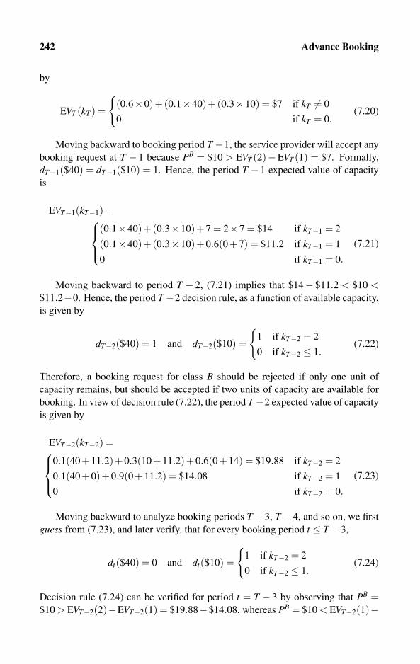
242 Advance Booking
by
EVT (kT ) =
{(0.6×0)+(0.1×40)+(0.3×10) = $7 if kT �= 0
0 if kT = 0.(7.20)
Moving backward to booking period T −1, the service provider will accept any
booking request at T − 1 because PB = $10 > EVT (2)−EVT (1) = $7. Formally,
dT−1($40) = dT−1($10) = 1. Hence, the period T − 1 expected value of capacity
is
EVT−1(kT−1) =⎧⎪⎨⎪⎩
(0.1×40)+(0.3×10)+7 = 2×7 = $14 if kT−1 = 2
(0.1×40)+(0.3×10)+0.6(0+7) = $11.2 if kT−1 = 1
0 if kT−1 = 0.
(7.21)
Moving backward to period T − 2, (7.21) implies that $14− $11.2 < $10 <$11.2−0. Hence, the period T−2 decision rule, as a function of available capacity,
is given by
dT−2($40) = 1 and dT−2($10) =
{1 if kT−2 = 2
0 if kT−2 ≤ 1.(7.22)
Therefore, a booking request for class B should be rejected if only one unit of
capacity remains, but should be accepted if two units of capacity are available for
booking. In view of decision rule (7.22), the period T−2 expected value of capacity
is given by
EVT−2(kT−2) =⎧⎪⎨⎪⎩
0.1(40+11.2)+0.3(10+11.2)+0.6(0+14) = $19.88 if kT−2 = 2
0.1(40+0)+0.9(0+11.2) = $14.08 if kT−2 = 1
0 if kT−2 = 0.
(7.23)
Moving backward to analyze booking periods T −3, T −4, and so on, we first
guess from (7.23), and later verify, that for every booking period t ≤ T −3,
dt($40) = 0 and dt($10) =
{1 if kT−2 = 2
0 if kT−2 ≤ 1.(7.24)
Decision rule (7.24) can be verified for period t = T − 3 by observing that PB =$10 > EVT−2(2)−EVT−2(1) = $19.88−$14.08, whereas PB = $10 < EVT−2(1)−
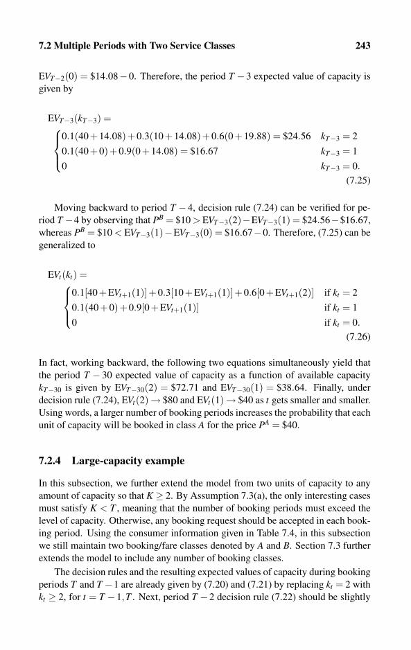
7.2 Multiple Periods with Two Service Classes 243
EVT−2(0) = $14.08−0. Therefore, the period T −3 expected value of capacity is
given by
EVT−3(kT−3) =⎧⎪⎨⎪⎩
0.1(40+14.08)+0.3(10+14.08)+0.6(0+19.88) = $24.56 kT−3 = 2
0.1(40+0)+0.9(0+14.08) = $16.67 kT−3 = 1
0 kT−3 = 0.
(7.25)
Moving backward to period T − 4, decision rule (7.24) can be verified for pe-
riod T −4 by observing that PB = $10 > EVT−3(2)−EVT−3(1) = $24.56−$16.67,
whereas PB = $10 < EVT−3(1)−EVT−3(0) = $16.67−0. Therefore, (7.25) can be
generalized to
EVt(kt) =⎧⎪⎨⎪⎩
0.1[40+EVt+1(1)]+0.3[10+EVt+1(1)]+0.6[0+EVt+1(2)] if kt = 2
0.1(40+0)+0.9[0+EVt+1(1)] if kt = 1
0 if kt = 0.
(7.26)
In fact, working backward, the following two equations simultaneously yield that
the period T − 30 expected value of capacity as a function of available capacity
kT−30 is given by EVT−30(2) = $72.71 and EVT−30(1) = $38.64. Finally, under
decision rule (7.24), EVt(2)→ $80 and EVt(1)→ $40 as t gets smaller and smaller.
Using words, a larger number of booking periods increases the probability that each
unit of capacity will be booked in class A for the price PA = $40.
7.2.4 Large-capacity example
In this subsection, we further extend the model from two units of capacity to any
amount of capacity so that K ≥ 2. By Assumption 7.3(a), the only interesting cases
must satisfy K < T , meaning that the number of booking periods must exceed the
level of capacity. Otherwise, any booking request should be accepted in each book-
ing period. Using the consumer information given in Table 7.4, in this subsection
we still maintain two booking/fare classes denoted by A and B. Section 7.3 further
extends the model to include any number of booking classes.
The decision rules and the resulting expected values of capacity during booking
periods T and T −1 are already given by (7.20) and (7.21) by replacing kt = 2 with
kt ≥ 2, for t = T −1,T . Next, period T −2 decision rule (7.22) should be slightly

244 Advance Booking
modified to
dT−2($40) = 1 and dT−2($10) =
⎧⎪⎨⎪⎩
1 if kT−2 ≥ 3
1 if kT−2 = 2
0 if kT−2 ≤ 1.
(7.27)
Clearly, if kT−2 = 3, any booking request should be accepted, as this capacity level
equals exactly the number of remaining booking periods. Therefore, the period T−2 expected value of capacity is given by
EVT−2(kT−2) =⎧⎪⎪⎪⎪⎨⎪⎪⎪⎪⎩
(0.1×40)+(0.3×10)+14 = 3×7 = $21 if kT−2 ≥ 3
0.1(40+11.2)+0.3(10+11.2)+0.6(0+14) = $19.88 if kT−2 = 2
0.1(40+0)+0.9(0+11.2) = $14.08 if kT−2 = 1
0 if kT−2 = 0.
(7.28)
The first line in (7.28) corresponds to excess capacity relative to the number of
booking periods in which any booking request is accepted. Other cases are identical
to those given by (7.23).
Moving backward to analyze booking periods T −3, T −4, and so on, we can
first guess from (7.28) and later verify that for every booking period t ≤ T −3,
dt($40) = 0 and dt($10) =
{1 if kT−2 ≥ 2
0 if kT−2 ≤ 1.(7.29)
Decision rule (7.29) is verified for period t = T − 3 by observing that PB =$10 > EVT−2(3)−EVT−2(2) = $21−$19.88, PB = $10 > EVT−2(2)−EVT−2(1) =$19.88−$14.08, and PB = $10 < EVT−2(1)−EVT−2(0) = $14.08−0. Therefore,
the period T −3 expected value of capacity is given by
EVT−3(kT−3) =⎧⎪⎪⎪⎪⎪⎪⎨⎪⎪⎪⎪⎪⎪⎩
(0.1×40)+(0.3×10)+21 = 4×7 = $28 kT−3 ≥ 4
0.1(40+19.88)+0.3(10+19.88)+0.6(0+21) = $27.55 kT−3 = 3
0.1(40+14.08)+0.3(10+14.08)+0.6(0+19.88) = $24.56 kT−3 = 2
0.1(40+0)+0.9(0+14.08) = $16.67 kT−3 = 1
0 kT−3 = 0.
(7.30)
Moving backward to period T − 4, decision rule (7.29) can be verified for pe-
riod T − 4 by observing that PB = $10 > EVT−3(4)−EVT−3(3) = $28− $27.55,
PB = $10 > EVT−3(3)− EVT−3(2) = $27.55− 24.56, PB = $10 > EVT−3(2)−
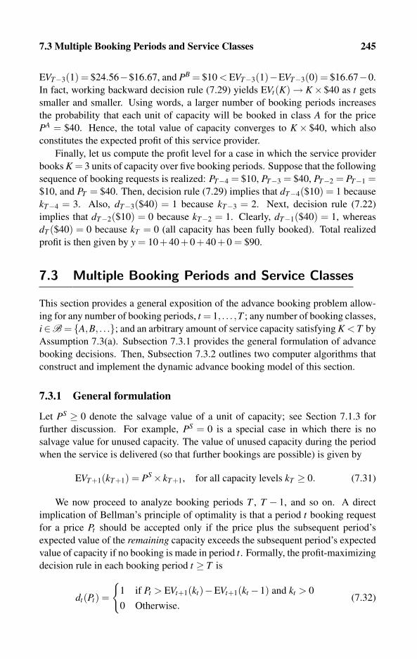
7.3 Multiple Booking Periods and Service Classes 245
EVT−3(1) = $24.56−$16.67, and PB = $10 < EVT−3(1)−EVT−3(0) = $16.67−0.
In fact, working backward decision rule (7.29) yields EVt(K)→ K×$40 as t gets
smaller and smaller. Using words, a larger number of booking periods increases
the probability that each unit of capacity will be booked in class A for the price
PA = $40. Hence, the total value of capacity converges to K × $40, which also
constitutes the expected profit of this service provider.
Finally, let us compute the profit level for a case in which the service provider
books K = 3 units of capacity over five booking periods. Suppose that the following
sequence of booking requests is realized: PT−4 = $10, PT−3 = $40, PT−2 = PT−1 =$10, and PT = $40. Then, decision rule (7.29) implies that dT−4($10) = 1 because
kT−4 = 3. Also, dT−3($40) = 1 because kT−3 = 2. Next, decision rule (7.22)
implies that dT−2($10) = 0 because kT−2 = 1. Clearly, dT−1($40) = 1, whereas
dT ($40) = 0 because kT = 0 (all capacity has been fully booked). Total realized
profit is then given by y = 10+40+0+40+0 = $90.
7.3 Multiple Booking Periods and Service Classes
This section provides a general exposition of the advance booking problem allow-
ing for any number of booking periods, t = 1, . . . ,T ; any number of booking classes,
i∈B = {A,B, . . .}; and an arbitrary amount of service capacity satisfying K < T by
Assumption 7.3(a). Subsection 7.3.1 provides the general formulation of advance
booking decisions. Then, Subsection 7.3.2 outlines two computer algorithms that
construct and implement the dynamic advance booking model of this section.
7.3.1 General formulation
Let PS ≥ 0 denote the salvage value of a unit of capacity; see Section 7.1.3 for
further discussion. For example, PS = 0 is a special case in which there is no
salvage value for unused capacity. The value of unused capacity during the period
when the service is delivered (so that further bookings are possible) is given by
EVT+1(kT+1) = PS× kT+1, for all capacity levels kT ≥ 0. (7.31)
We now proceed to analyze booking periods T , T − 1, and so on. A direct
implication of Bellman’s principle of optimality is that a period t booking request
for a price Pt should be accepted only if the price plus the subsequent period’s
expected value of the remaining capacity exceeds the subsequent period’s expected
value of capacity if no booking is made in period t. Formally, the profit-maximizing
decision rule in each booking period t ≥ T is
dt(Pt) =
{1 if Pt > EVt+1(kt)−EVt+1(kt −1) and kt > 0
0 Otherwise.(7.32)
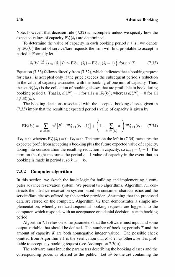
246 Advance Booking
Note, however, that decision rule (7.32) is incomplete unless we specify how the
expected values of capacity EVt(kt) are determined.
To determine the value of capacity in each booking period t ≤ T , we denote
by Bt(kt) the set of service/fare requests the firm will find profitable to accept in
period t. Formally let
Bt(kt)def={
i ∈B∣∣ Pi > EVt+1(kt)−EVt+1(kt −1)
}for t ≤ T. (7.33)
Equation (7.33) follows directly from (7.32), which indicates that a booking request
for class i is accepted only if the price exceeds the subsequent period’s reduction
in the value of capacity associated with the booking of one unit of capacity. Thus,
the set Bt(kt) is the collection of booking classes that are profitable to book during
booking period t. That is, dt(Pi) = 1 for all i ∈Bt(kt), whereas dt(Pi) = 0 for all
i �∈Bt(kt).The booking decisions associated with the accepted booking classes given in
(7.33) imply that the resulting expected period t value of capacity is given by
EVt(kt) = ∑i∈Bt(kt)
π i [Pi +EVt+1(kt −1)]+
(1− ∑
i∈Bt(kt)π i
)EVt+1(kt) (7.34)
if kt > 0, whereas EVt(kt) = 0 if kt = 0. The term on the left in (7.34) measures the
expected profit from accepting a booking plus the future expected value of capacity,
taking into consideration the resulting reduction in capacity, so kt+1 = kt −1. The
term on the right measures the period t + 1 value of capacity in the event that no
booking is made in period t, so kt+1 = kt .
7.3.2 Computer algorithm
In this section, we sketch the basic logic for building and implementing a com-
puter advance reservation system. We present two algorithms. Algorithm 7.1 con-
structs the advance reservation system based on consumer characteristics and the
service/fare classes offered by the service provider. Assuming that the processed
data are stored on the computer, Algorithm 7.2 then demonstrates a simple im-
plementation, whereby realized sequential booking requests are logged into the
computer, which responds with an acceptance or a denial decision in each booking
period.
Algorithm 7.1 relies on some parameters that the software must input and some
output variable that should be defined. The number of booking periods T and the
amount of capacity K are both nonnegative integer valued. One possible check
omitted from Algorithm 7.1 is the verification that K < T , as otherwise it is prof-
itable to accept any booking request (see Assumption 7.3(a)).
The software must input the parameters describing the booking classes and the
corresponding prices as offered to the public. Let B be the set containing the
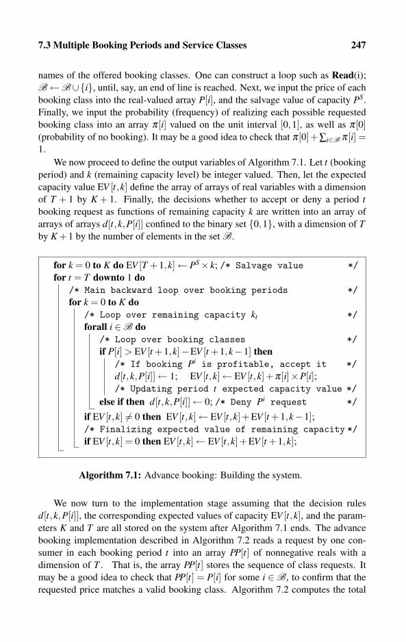
7.3 Multiple Booking Periods and Service Classes 247
names of the offered booking classes. One can construct a loop such as Read(i);
B←B∪{i}, until, say, an end of line is reached. Next, we input the price of each
booking class into the real-valued array P[i], and the salvage value of capacity PS.
Finally, we input the probability (frequency) of realizing each possible requested
booking class into an array π[i] valued on the unit interval [0,1], as well as π[0](probability of no booking). It may be a good idea to check that π[0]+∑i∈B π[i] =1.
We now proceed to define the output variables of Algorithm 7.1. Let t (booking
period) and k (remaining capacity level) be integer valued. Then, let the expected
capacity value EV [t,k] define the array of arrays of real variables with a dimension
of T + 1 by K + 1. Finally, the decisions whether to accept or deny a period tbooking request as functions of remaining capacity k are written into an array of
arrays of arrays d[t,k,P[i]] confined to the binary set {0,1}, with a dimension of Tby K +1 by the number of elements in the set B.
for k = 0 to K do EV [T +1,k]← PS× k; /* Salvage value */for t = T downto 1 do
/* Main backward loop over booking periods */for k = 0 to K do
/* Loop over remaining capacity kt */forall i ∈B do
/* Loop over booking classes */if P[i] > EV [t +1,k]−EV [t +1,k−1] then
/* If booking Pi is profitable, accept it */d[t,k,P[i]]← 1; EV [t,k]← EV [t,k]+π[i]×P[i];/* Updating period t expected capacity value */
else if then d[t,k,P[i]]← 0; /* Deny Pi request */
if EV [t,k] �= 0 then EV [t,k]← EV [t,k]+EV [t +1,k−1];/* Finalizing expected value of remaining capacity */if EV [t,k] = 0 then EV [t,k]← EV [t,k]+EV [t +1,k];
Algorithm 7.1: Advance booking: Building the system.
We now turn to the implementation stage assuming that the decision rules
d[t,k,P[i]], the corresponding expected values of capacity EV [t,k], and the param-
eters K and T are all stored on the system after Algorithm 7.1 ends. The advance
booking implementation described in Algorithm 7.2 reads a request by one con-
sumer in each booking period t into an array PP[t] of nonnegative reals with a
dimension of T . That is, the array PP[t] stores the sequence of class requests. It
may be a good idea to check that PP[t] = P[i] for some i ∈B, to confirm that the
requested price matches a valid booking class. Algorithm 7.2 computes the total
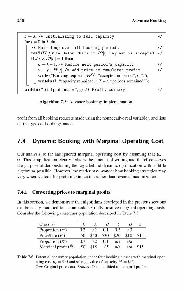
248 Advance Booking
k← K; /* Initializing to full capacity */for t = 0 to T do
/* Main loop over all booking periods */read (PP[t]); /* Below check if PP[t] request is accepted */if d[t,k,PP[i]] = 1 then
k← k−1; /* Reduce next period’s capacity */y← y+PP[t]; /* Add price to cumulated profit */write (“Booking request”, PP[t], “accepted in period”, t, “.”);
writeln (k, “capacity remained.”, T − t, “periods remained.”);
writeln (“Total profit made:”, y); /* Profit summary */
Algorithm 7.2: Advance booking: Implementation.
profit from all booking requests made using the nonnegative real variable y and lists
all the types of bookings made.
7.4 Dynamic Booking with Marginal Operating Cost
Our analysis so far has ignored marginal operating cost by assuming that μo =0. This simplification clearly reduces the amount of writing and therefore serves
the purpose of demonstrating the logic behind dynamic optimization with as little
algebra as possible. However, the reader may wonder how booking strategies may
vary when we look for profit maximization rather than revenue maximization.
7.4.1 Converting prices to marginal profits
In this section, we demonstrate that algorithms developed in the previous sections
can be easily modified to accommodate strictly positive marginal operating costs.
Consider the following consumer population described in Table 7.5.
Class (i) 0 A B C D SProportion (π i) 0.2 0.2 0.1 0.2 0.3
Price/fare (Pi) $0 $40 $30 $20 $10 $15
Proportion (π i) 0.7 0.2 0.1 n/a n/a
Marginal profit (Pi) $0 $15 $5 n/a n/a $15
Table 7.5: Potential consumer population under four booking classes with marginal oper-
ating cost μo = $25 and salvage value of capacity PS = $15.
Top: Original price data. Bottom: Data modified to marginal profits.
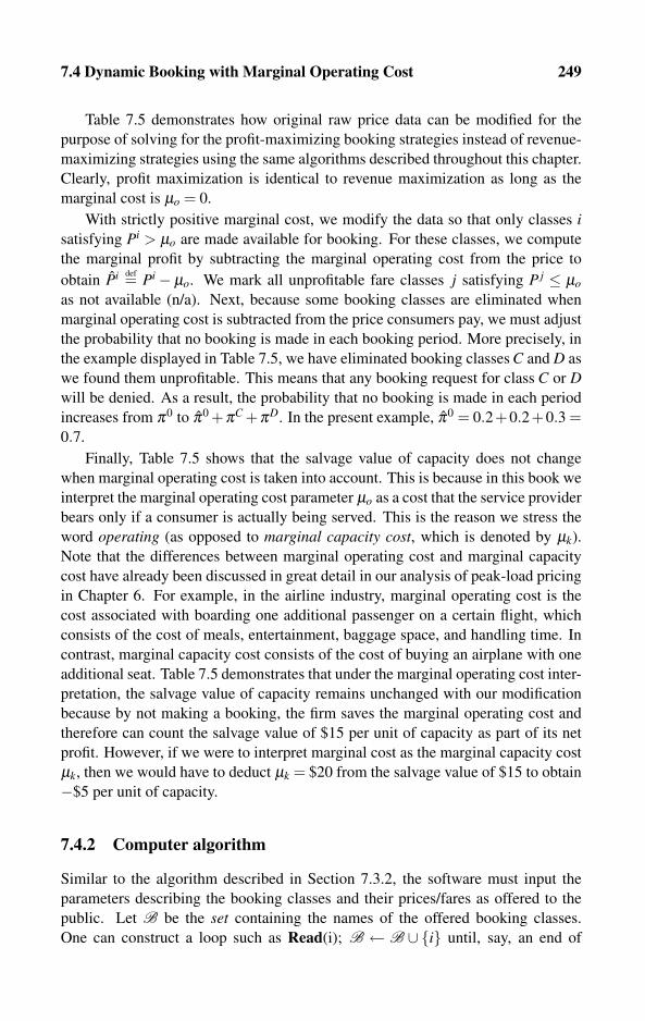
7.4 Dynamic Booking with Marginal Operating Cost 249
Table 7.5 demonstrates how original raw price data can be modified for the
purpose of solving for the profit-maximizing booking strategies instead of revenue-
maximizing strategies using the same algorithms described throughout this chapter.
Clearly, profit maximization is identical to revenue maximization as long as the
marginal cost is μo = 0.
With strictly positive marginal cost, we modify the data so that only classes isatisfying Pi > μo are made available for booking. For these classes, we compute
the marginal profit by subtracting the marginal operating cost from the price to
obtain Pi def= Pi− μo. We mark all unprofitable fare classes j satisfying P j ≤ μo
as not available (n/a). Next, because some booking classes are eliminated when
marginal operating cost is subtracted from the price consumers pay, we must adjust
the probability that no booking is made in each booking period. More precisely, in
the example displayed in Table 7.5, we have eliminated booking classes C and D as
we found them unprofitable. This means that any booking request for class C or Dwill be denied. As a result, the probability that no booking is made in each period
increases from π0 to π0 +πC +πD. In the present example, π0 = 0.2+0.2+0.3 =0.7.
Finally, Table 7.5 shows that the salvage value of capacity does not change
when marginal operating cost is taken into account. This is because in this book we
interpret the marginal operating cost parameter μo as a cost that the service provider
bears only if a consumer is actually being served. This is the reason we stress the
word operating (as opposed to marginal capacity cost, which is denoted by μk).
Note that the differences between marginal operating cost and marginal capacity
cost have already been discussed in great detail in our analysis of peak-load pricing
in Chapter 6. For example, in the airline industry, marginal operating cost is the
cost associated with boarding one additional passenger on a certain flight, which
consists of the cost of meals, entertainment, baggage space, and handling time. In
contrast, marginal capacity cost consists of the cost of buying an airplane with one
additional seat. Table 7.5 demonstrates that under the marginal operating cost inter-
pretation, the salvage value of capacity remains unchanged with our modification
because by not making a booking, the firm saves the marginal operating cost and
therefore can count the salvage value of $15 per unit of capacity as part of its net
profit. However, if we were to interpret marginal cost as the marginal capacity cost
μk, then we would have to deduct μk = $20 from the salvage value of $15 to obtain
−$5 per unit of capacity.
7.4.2 Computer algorithm
Similar to the algorithm described in Section 7.3.2, the software must input the
parameters describing the booking classes and their prices/fares as offered to the
public. Let B be the set containing the names of the offered booking classes.
One can construct a loop such as Read(i); B ← B ∪ {i} until, say, an end of

250 Advance Booking
line is reached. Next, we input the marginal operating cost μo and the price of
each booking class into the real valued array P[i], as well as the salvage value of
capacity PS. Finally, we input the probability (frequency) of realizing each possible
requested booking class into an array π[i] valued on the unit interval [0,1], as well
as π[0] (probability of no booking). It is useful to perform a check that π[0] +∑i∈B π[i] = 1. The program suggested in Algorithm 7.3 transforms the above input
into the corresponding modified variables, which we denote by B and π[0].
forall i ∈B do/* Main loop over available booking classes */if P[i] > μo then
/* If booking Pi exceeds marginal cost */
B← B∪{i}; /* Add i to new set of bookable classes */
else if thenπ0← π0 +π i/* Update probability of no booking */
forall i ∈ B do/* Writing: Loop over adjusted bookable classes */writeln (“Booking price”, P[i], “yields marginal profit of”, P[i]−μo, “is
requested with probability” π[i]);write (“Adjusted probability of no booking is”, π0);
Algorithm 7.3: Advance booking: Marginal operating cost.
7.5 Network-based Dynamic Advance Booking
Our analysis so far has assumed that services use specific capacity that is not used
by other services provided by the firm. In this section, we relax this assumption and
assume that capacity can be used to provide other complementary services. Thus,
accepting a booking request for one service may reduce the amount of capacity
available for other services. This implies that an advance reservation system must
compute the trade-off between the extra revenue generated by an acceptance of a
booking request for one service and the potential revenue loss not only from the
reduction in capacity of the same service but also from the potential reduction in
revenue from complementary services. For earlier scientific literature on network
yield management, see Glover, Glover, Lorenzo, and McMillan (1982) and Wang
(1983). Additional references are provided in Talluri and van Ryzin (2004, Ch. 3).
To take a specific case, consider an airline serving three cities labeled A, B, and
H. Passengers seek to book tickets for traveling from city A to H, H to B, and A to
B. These cities and the desired connections are depicted in Figure 7.1.

7.5 Network-based Dynamic Advance Booking 251
��
��
��
��
��
��
H
A B
��
��
Figure 7.1: Booking airline tickets under a hub-and-spokes network.
For the sake of demonstration only, we ignore return flights and round-trip tick-
ets. The connections displayed in Figure 7.1 are commonly referred to as forming
a hub-and-spokes network. City H serves as a hub if there is no direct connection
between cities A and B.
Suppose that the airline company does not provide a direct connection be-
tween A and B, which means that passengers on the route from A to B have to
first board the flight from A to H, and then change to the flight from H to B. The
airline allocates KAH units of capacity (number of seats in the present example) for
the route AH, and KHB units of capacity for the route HB. Clearly, these capacity
allocations serve two types of passengers: passengers who wish to travel to and
from the hub city H (A to H and H to B in the present example) and those traveling
between non-hub cities (A to B in the present example).
7.5.1 A numerical example
Consider the single-airline three-city example illustrated in Figure 7.1. There are
two booking periods labeled t = 1,2. All flights take off during period t = 3, after
the booking periods end. Suppose that on each flight there is only one unit of
capacity. Formally, let KAH = KHB = 1. Table 7.6 describes passengers wishing to
travel on these three routes.
Route (i) 0 AH HB ABProportion (π i) 0.1 0.2 0.2 0.5
Airfare (Pi) $0 $20 $30 $40
Table 7.6: Passengers on a hub-and-spokes network. Note: Route 0 refers to passengers
who end up not booking any flight.
The fractions in Table 7.6 refer to the proportion of passengers out of the entire
potential passenger population who wish to travel on a certain route. As before,
we also interpret these fractions as probabilities of making a booking on a certain
route. The airfares on these routes are denoted by PAB, PAH , and PHB. Models of
this sort generally assume that PAB < PAH + PHB, as otherwise a passenger to or
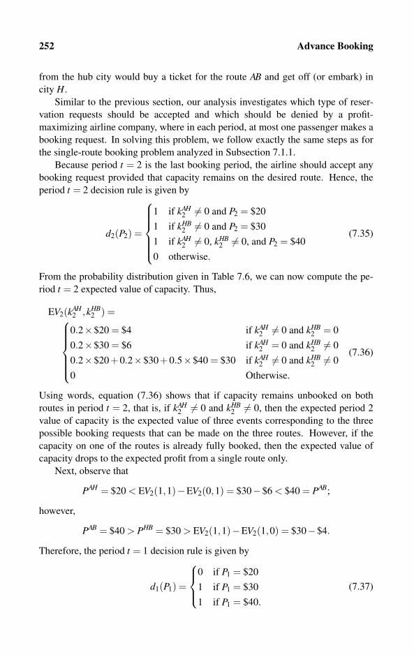
252 Advance Booking
from the hub city would buy a ticket for the route AB and get off (or embark) in
city H.
Similar to the previous section, our analysis investigates which type of reser-
vation requests should be accepted and which should be denied by a profit-
maximizing airline company, where in each period, at most one passenger makes a
booking request. In solving this problem, we follow exactly the same steps as for
the single-route booking problem analyzed in Subsection 7.1.1.
Because period t = 2 is the last booking period, the airline should accept any
booking request provided that capacity remains on the desired route. Hence, the
period t = 2 decision rule is given by
d2(P2) =
⎧⎪⎪⎪⎪⎨⎪⎪⎪⎪⎩
1 if kAH2 �= 0 and P2 = $20
1 if kHB2 �= 0 and P2 = $30
1 if kAH2 �= 0, kHB
2 �= 0, and P2 = $40
0 otherwise.
(7.35)
From the probability distribution given in Table 7.6, we can now compute the pe-
riod t = 2 expected value of capacity. Thus,
EV2(kAH2 ,kHB
2 ) =⎧⎪⎪⎪⎪⎨⎪⎪⎪⎪⎩
0.2×$20 = $4 if kAH2 �= 0 and kHB
2 = 0
0.2×$30 = $6 if kAH2 = 0 and kHB
2 �= 0
0.2×$20+0.2×$30+0.5×$40 = $30 if kAH2 �= 0 and kHB
2 �= 0
0 Otherwise.
(7.36)
Using words, equation (7.36) shows that if capacity remains unbooked on both
routes in period t = 2, that is, if kAH2 �= 0 and kHB
2 �= 0, then the expected period 2
value of capacity is the expected value of three events corresponding to the three
possible booking requests that can be made on the three routes. However, if the
capacity on one of the routes is already fully booked, then the expected value of
capacity drops to the expected profit from a single route only.
Next, observe that
PAH = $20 < EV2(1,1)−EV2(0,1) = $30−$6 < $40 = PAB;
however,
PAB = $40 > PHB = $30 > EV2(1,1)−EV2(1,0) = $30−$4.
Therefore, the period t = 1 decision rule is given by
d1(P1) =
⎧⎪⎨⎪⎩
0 if P1 = $20
1 if P1 = $30
1 if P1 = $40.
(7.37)
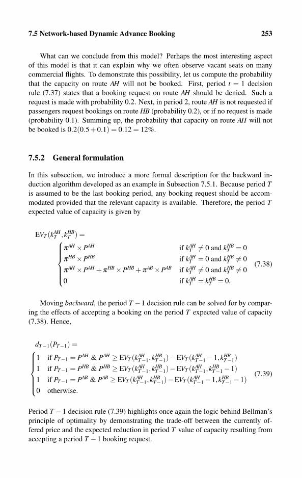
7.5 Network-based Dynamic Advance Booking 253
What can we conclude from this model? Perhaps the most interesting aspect
of this model is that it can explain why we often observe vacant seats on many
commercial flights. To demonstrate this possibility, let us compute the probability
that the capacity on route AH will not be booked. First, period t = 1 decision
rule (7.37) states that a booking request on route AH should be denied. Such a
request is made with probability 0.2. Next, in period 2, route AH is not requested if
passengers request bookings on route HB (probability 0.2), or if no request is made
(probability 0.1). Summing up, the probability that capacity on route AH will not
be booked is 0.2(0.5+0.1) = 0.12 = 12%.
7.5.2 General formulation
In this subsection, we introduce a more formal description for the backward in-
duction algorithm developed as an example in Subsection 7.5.1. Because period Tis assumed to be the last booking period, any booking request should be accom-
modated provided that the relevant capacity is available. Therefore, the period Texpected value of capacity is given by
EVT (kAHT ,kHB
T ) =⎧⎪⎪⎪⎪⎨⎪⎪⎪⎪⎩
πAH ×PAH if kAHT �= 0 and kHB
T = 0
πHB×PHB if kAHT = 0 and kHB
T �= 0
πAH ×PAH +πHB×PHB +πAB×PAB if kAHT �= 0 and kHB
T �= 0
0 if kAHT = kHB
T = 0.
(7.38)
Moving backward, the period T −1 decision rule can be solved for by compar-
ing the effects of accepting a booking on the period T expected value of capacity
(7.38). Hence,
dT−1(PT−1) =⎧⎪⎪⎪⎪⎨⎪⎪⎪⎪⎩
1 if PT−1 = PAH & PAH ≥ EVT (kAHT−1,k
HBT−1)−EVT (kAH
T−1−1,kHBT−1)
1 if PT−1 = PHB & PHB ≥ EVT (kAHT−1,k
HBT−1)−EVT (kAH
T−1,kHBT−1−1)
1 if PT−1 = PAB & PAB ≥ EVT (kAHT−1,k
HBT−1)−EVT (kAH
T−1−1,kHBT−1−1)
0 otherwise.
(7.39)
Period T −1 decision rule (7.39) highlights once again the logic behind Bellman’s
principle of optimality by demonstrating the trade-off between the currently of-
fered price and the expected reduction in period T value of capacity resulting from
accepting a period T −1 booking request.
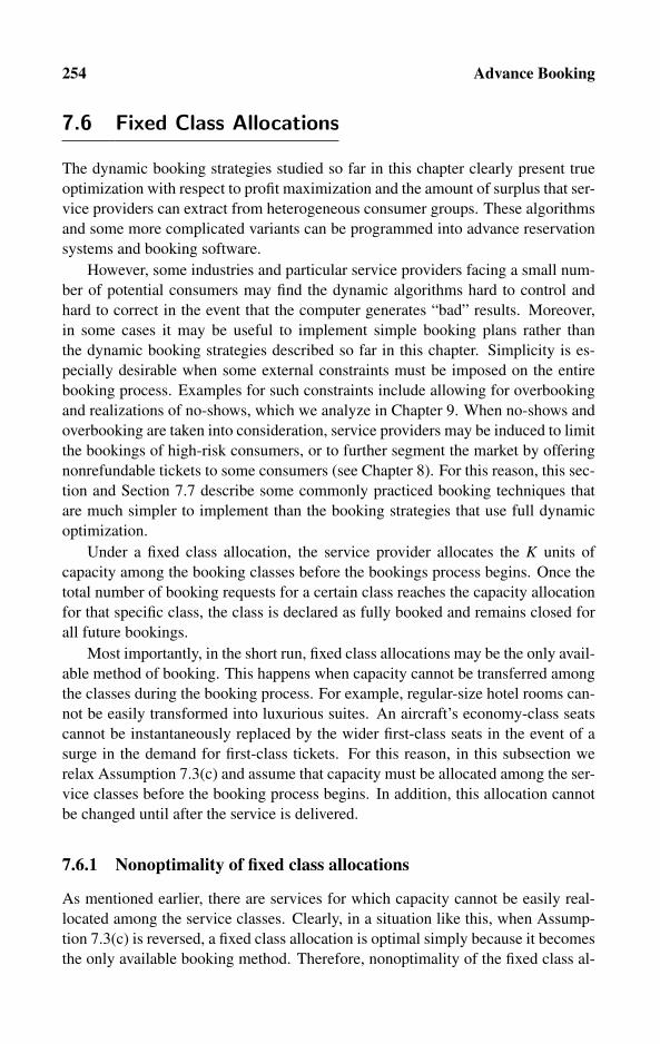
254 Advance Booking
7.6 Fixed Class Allocations
The dynamic booking strategies studied so far in this chapter clearly present true
optimization with respect to profit maximization and the amount of surplus that ser-
vice providers can extract from heterogeneous consumer groups. These algorithms
and some more complicated variants can be programmed into advance reservation
systems and booking software.
However, some industries and particular service providers facing a small num-
ber of potential consumers may find the dynamic algorithms hard to control and
hard to correct in the event that the computer generates “bad” results. Moreover,
in some cases it may be useful to implement simple booking plans rather than
the dynamic booking strategies described so far in this chapter. Simplicity is es-
pecially desirable when some external constraints must be imposed on the entire
booking process. Examples for such constraints include allowing for overbooking
and realizations of no-shows, which we analyze in Chapter 9. When no-shows and
overbooking are taken into consideration, service providers may be induced to limit
the bookings of high-risk consumers, or to further segment the market by offering
nonrefundable tickets to some consumers (see Chapter 8). For this reason, this sec-
tion and Section 7.7 describe some commonly practiced booking techniques that
are much simpler to implement than the booking strategies that use full dynamic
optimization.
Under a fixed class allocation, the service provider allocates the K units of
capacity among the booking classes before the bookings process begins. Once the
total number of booking requests for a certain class reaches the capacity allocation
for that specific class, the class is declared as fully booked and remains closed for
all future bookings.
Most importantly, in the short run, fixed class allocations may be the only avail-
able method of booking. This happens when capacity cannot be transferred among
the classes during the booking process. For example, regular-size hotel rooms can-
not be easily transformed into luxurious suites. An aircraft’s economy-class seats
cannot be instantaneously replaced by the wider first-class seats in the event of a
surge in the demand for first-class tickets. For this reason, in this subsection we
relax Assumption 7.3(c) and assume that capacity must be allocated among the ser-
vice classes before the booking process begins. In addition, this allocation cannot
be changed until after the service is delivered.
7.6.1 Nonoptimality of fixed class allocations
As mentioned earlier, there are services for which capacity cannot be easily real-
located among the service classes. Clearly, in a situation like this, when Assump-
tion 7.3(c) is reversed, a fixed class allocation is optimal simply because it becomes
the only available booking method. Therefore, nonoptimality of the fixed class al-
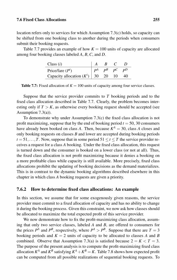
7.6 Fixed Class Allocations 255
location refers only to services for which Assumption 7.3(c) holds, so capacity can
be shifted from one booking class to another during the periods when consumers
submit their booking requests.
Table 7.7 provides an example of how K = 100 units of capacity are allocated
among four booking classes labeled A, B, C, and D.
Class (i) A B C D
Price/fare (Pi) PA PB PC PD
Capacity allocation (Ki) 30 20 10 40
Table 7.7: Fixed allocation of K = 100 units of capacity among four service classes.
Suppose that the service provider commits to T booking periods and to the
fixed class allocation described in Table 7.7. Clearly, the problem becomes inter-
esting only if T > K, as otherwise every booking request should be accepted (see
Assumption 7.3(a)).
To demonstrate why under Assumption 7.3(c) the fixed class allocation is not
profit maximizing, suppose that by the end of booking period t = 50, 30 consumers
have already been booked on class A. Then, because KA = 30, class A closes and
only booking requests on classes B and lower are accepted during booking periods
t = 51, . . . ,T . Now, suppose that in some period 51≤ t ≤ T the service provider re-
ceives a request for a class A booking. Under the fixed class allocation, this request
is turned down and the consumer is booked on a lower class (or not at all). Thus,
the fixed class allocation is not profit maximizing because it denies a booking on
a more profitable class while capacity is still available. More precisely, fixed class
allocations prohibit the updating of booking decisions as the demand materializes.
This is in contrast to the dynamic booking algorithms described elsewhere in this
chapter in which class A booking requests are given a priority.
7.6.2 How to determine fixed class allocations: An example
In this section, we assume that for some exogenously given reasons, the service
provider must commit to a fixed allocation of capacity and has no ability to change
it during the booking process. Given this constraint, we now ask how classes should
be allocated to maximize the total expected profit of this service provider.
We now demonstrate how to fix the profit-maximizing class allocation, assum-
ing that only two service classes, labeled A and B, are offered to consumers for
the prices PA and PB, respectively, where PA > PB. Suppose that there are T = 3
booking periods and K = 2 units of capacity to be allocated to classes A and Bcombined. Observe that Assumption 7.3(a) is satisfied because 2 = K < T = 3.
The purpose of the present analysis is to compute the profit-maximizing fixed class
allocation KA and KB satisfying KA +KB = K. Table 7.8 shows how expected profit
can be computed from all possible realizations of sequential booking requests. To
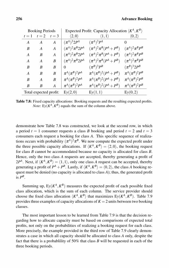
256 Advance Booking
Booking Periods Expected Profit: Capacity Allocation 〈KA,KB〉t = 1 t = 2 t = 3 〈2,0〉 〈1,1〉 〈0,2〉
A A A (πA)32PA (πA)3PA 0
B A A (πA)2πB2PA (πA)2πB(PA +PB) (πA)2πBPB
A B A (πA)2πB2PA (πA)2πB(PA +PB) (πA)2πBPB
A A B (πA)2πB2PA (πA)2πB(PA +PB) (πA)2πBPB
B B B 0 (πB)3PB (πB)32PB
A B B πA(πB)2PA πA(πB)2(PA +PB) πA(πB)2PB
B A B πA(πB)2PA πA(πB)2(PA +PB) πA(πB)2PB
B B A πA(πB)2PA πA(πB)2(PA +PB) πA(πB)2PB
Total expected profit: Ey(2,0) Ey(1,1) Ey(0,2)
Table 7.8: Fixed capacity allocations: Booking requests and the resulting expected profits.
Note: Ey(KA,KB) equals the sum of the column above.
demonstrate how Table 7.8 was constructed, we look at the second row, in which
a period t = 1 consumer requests a class B booking and period t = 2 and t = 3
consumers each request a booking for class A. This specific sequence of realiza-
tions occurs with probability (πA)2πB. We now compute the expected profit under
the three possible capacity allocations. If 〈KA,KB〉 = 〈2,0〉, the booking request
for class B cannot be accommodated because no capacity is allocated for class B.
Hence, only the two class A requests are accepted, thereby generating a profit of
2PA. Next, if 〈KA,KB〉= 〈1,1〉, only one class A request can be accepted, thereby
generating a profit of PA +PB. Lastly, if 〈KA,KB〉= 〈0,2〉, the class A booking re-
quest must be denied (no capacity is allocated to class A); thus, the generated profit
is PB.
Summing up, Ey(KA,KB) measures the expected profit of each possible fixed
class allocation, which is the sum of each column. The service provider should
choose the fixed class allocation 〈KA,KB〉 that maximizes Ey(KA,KB). Table 7.9
provides three examples of capacity allocations of K = 2 units between two booking
classes.
The most important lesson to be learned from Table 7.9 is that the decision re-
garding how to allocate capacity must be based on comparisons of expected total
profits, not only on the probabilities of realizing a booking request for each class.
More precisely, the example provided in the third row of Table 7.9 clearly demon-
strates a case in which all capacity should be allocated to class A only, despite the
fact that there is a probablility of 50% that class B will be requested in each of the
three booking periods.

7.6 Fixed Class Allocations 257
Booking Data Capacity Allocation Profitable
PA PB πA πB 〈2,0〉 〈1,1〉 〈0,2〉 Choice
$30 $10 0.1 0.9 $8.97 $18.12 $19.71 〈0,2〉$20 $10 0.1 0.9 $5.98 $15.41 $19.71 〈1,1〉$30 $10 0.5 0.5 $41.25 $35.00 $13.75 〈2,0〉
Table 7.9: Examples of profit-maximizing fixed class allocations, based on specific data
inserted into Table 7.8. Total capacity equals K = 2.
7.6.3 Computer algorithm for fixed class allocations
We now sketch a brief computer algorithm for finding the fixed class allocation
that maximizes expected profit. The following parameter and variable definitions
should be declared at the beginning of the program: B, a finite set of all booking
classes, that is, B = A,B, . . . , i, . . .; the price vector P[i] for every booking class
i∈B; and π[i], the corresponding probability that a consumer will submit a request
for booking on class i ∈B. The auxiliary integer valued vector component c[i] will
serve as a counter of how many bookings have been made on class i, i∈B. Finally,
the integer-valued parameter K inputs the capacity level, and T inputs the number
of booking periods.
The algorithm suggested below also omits two procedures (subroutines) for
generating two sets. Formally, the program should add a procedure for constructing
the set of all possible allocations of capacity among all booking classes that satisfy
Kdef=
{〈k[A],k[B], . . . ,k[i], . . .〉
∣∣∣∣∣ ∑i∈B
k[i] = K
}. (7.40)
For example, if A and B are the only booking classes,
K = {〈K,0〉,〈K−1,1〉,〈K−2,2〉, . . . ,〈0,K〉} .
Elements of the set K are denoted by the vectors�k ∈K and max�k ∈K .
The program should also include a procedure for constructing the set of all
possible realizations of booking requests according to their arrival period,
Rdef= {〈r[1],r[2], . . . ,r[t], . . . ,r[T ]〉 | r[t] ∈B} , (7.41)
where r[t] is the requested class during booking period t, t = 1, . . . ,T . An element
of the set R will be denoted by a vector �r ∈ R, which lists the realizations of
booking requests in the order they are received. For example, Table 7.8 has already
shown that if there are only T = 3 booking periods,
R = {〈AAA〉,〈BAA〉,〈ABA〉,〈AAB〉,〈BBB〉,〈ABB〉,〈BAB〉,〈BBA〉} .

258 Advance Booking
A probability of realizing a specific sequence of booking requests is captured
by the variable πr ∈ [0,1] defined by πr = π[r[1]]×π[r[2]]×·· ·×π[r[T ]], which is
the product of probabilities of sequential realizations of booking requests. Finally,
real-valued output variables measuring expected profits are denoted by y, yk, and
yr. All these parameters and variables are now implemented in Algorithm 7.4.
for�k ∈K do/* Main loop over all possible class allocations */
yk← 0; /* Initializing profit from allocation �k */for�r ∈R do
/* Loop over all possible booking realizations */yr← 0; /* Initializing profit from realization �r */for i ∈B do c[i]← 0/* Initializing counters */for t = 1 to T do πr← πr×π[r[t]]/* Realization Prob. */for t = 1 to T do
/* Registering feasible booking requests */if c[r[t]] < k[r[t]] then
/* If requested class r[t] is underbooked */c[r[t]]← c[r[t]]+1; yr← yr +πr×P[r[t]];/* Updating booking counter and exp. profit */
yk← yk + yr; /* Updating class alloc. profit */
if maxy < yk then/* If class �k is so far the most profitable */
maxy← yk; max�k←�k; /* Register solution �k */
for i ∈B do writeln (“Allocate”, max�k[i], “capacity for class”, i);write (“The expected profit from this class allocation is”, maxy);
Algorithm 7.4: Advance booking: Fixed class allocation. Note: The main
loops may have to be simplified as they reach high orders for a large number
of booking periods.
7.7 Nested Class Allocations
The advantage of the nested class allocation over the fixed class allocation, such as
the one described in Table 7.7, is that it can prevent a situation in which booking
requests for class A are being denied because the capacity allocated for class Ahas been fully booked, whereas some capacity allocated for lower classes remains
unbooked. A nested booking allocation always allows bookings at higher classes if
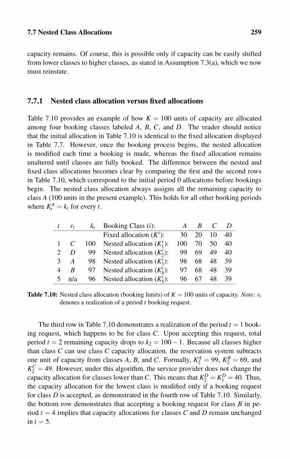
7.7 Nested Class Allocations 259
capacity remains. Of course, this is possible only if capacity can be easily shifted
from lower classes to higher classes, as stated in Assumption 7.3(a), which we now
must reinstate.
7.7.1 Nested class allocation versus fixed allocations
Table 7.10 provides an example of how K = 100 units of capacity are allocated
among four booking classes labeled A, B, C, and D. The reader should notice
that the initial allocation in Table 7.10 is identical to the fixed allocation displayed
in Table 7.7. However, once the booking process begins, the nested allocation
is modified each time a booking is made, whereas the fixed allocation remains
unaltered until classes are fully booked. The difference between the nested and
fixed class allocations becomes clear by comparing the first and the second rows
in Table 7.10, which correspond to the initial period 0 allocations before bookings
begin. The nested class allocation always assigns all the remaining capacity to
class A (100 units in the present example). This holds for all other booking periods
where KAt = kt for every t.
t rt kt Booking Class (i): A B C DFixed allocation (Ki): 30 20 10 40
1 C 100 Nested allocation (Ki1): 100 70 50 40
2 D 99 Nested allocation (Ki2): 99 69 49 40
3 A 98 Nested allocation (Ki3): 98 68 48 39
4 B 97 Nested allocation (Ki4): 97 68 48 39
5 n/a 96 Nested allocation (Ki5): 96 67 48 39
Table 7.10: Nested class allocation (booking limits) of K = 100 units of capacity. Note: rtdenotes a realization of a period t booking request.
The third row in Table 7.10 demonstrates a realization of the period t = 1 book-
ing request, which happens to be for class C. Upon accepting this request, total
period t = 2 remaining capacity drops to k2 = 100−1. Because all classes higher
than class C can use class C capacity allocation, the reservation system subtracts
one unit of capacity from classes A, B, and C. Formally, KA2 = 99, KB
2 = 69, and
KC2 = 49. However, under this algorithm, the service provider does not change the
capacity allocation for classes lower than C. This means that KD2 = KD
1 = 40. Thus,
the capacity allocation for the lowest class is modified only if a booking request
for class D is accepted, as demonstrated in the fourth row of Table 7.10. Similarly,
the bottom row demonstrates that accepting a booking request for class B in pe-
riod t = 4 implies that capacity allocations for classes C and D remain unchanged
in t = 5.

260 Advance Booking
7.7.2 How to determine nested class allocations: An example
We now modify the fixed class allocation example analyzed in Subsection 7.6.2
to nested class allocation. Using the exact same figures, Table 7.8 (fixed capacity
allocation) is now replaced with Table 7.11, which displays the expected profit from
each possible nested capacity allocation.
Periods Expected Profit: Nested Allocation of K = 2 Capacity
1 2 3 〈2,0〉 〈2,1〉 〈2,2〉A A A (πA)32PA (πA)32PA (πA)32PA
B A A (πA)2πB2PA (πA)2πB(PA +PB) (πA)2πB(PA +PB)A B A (πA)2πB2PA (πA)2πB(PA +PB) (πA)2πB(PA +PB)A A B (πA)2πB2PA (πA)2πB2PA (πA)2πB2PA
B B B (πB)30 (πB)3PB (πB)32PB
A B B πA(πB)2PA πA(πB)2(PA +PB) πA(πB)2(PA +PB)B A B πA(πB)2PA πA(πB)2(PA +PB) πA(πB)2(PA +PB)B B A πA(πB)2PA πA(πB)2(PA +PB) πA(πB)22PB
Profit: Ey(2,0) Ey(2,1) Ey(2,2)
Table 7.11: Nested capacity allocations: Booking requests and the resulting expected prof-
its. Note: Ey(KA,KB) is the sum of the columns above.
The columns of Table 7.11 display the expected profit of the three possible
nested allocations. The allocation 〈2,0〉 is identical to the fixed allocation in which
only class A bookings are allowed. Thus, expected profits are identical to those
given by Table 7.8. The nested allocation 〈2,1〉 implies that at most one booking
can be made on class B (but two bookings can be made on class A). The third
allocation 〈2,2〉 allows up to two bookings to be made on each class (but only two
bookings in total because K = 2).
Comparing the expected profit levels given in Table 7.8 with the profits dis-
played in Table 7.11 reveals that for some entries, the profits are equal and in some
others, the profits are higher under the nested capacity allocation. This leads us to
conclude that the nested capacity allocation is more profitable than the fixed ca-
pacity allocation. Table 7.12 displays three examples showing how expected profit
levels vary with all possible nested capacity allocations, given that total capacity
is restricted to K = 2. Comparing Table 7.12 with Table 7.9 clearly shows that
the nested capacity allocation yields a higher expected profit compared with the
fixed capacity allocation. Therefore, we can conclude that for every fixed capacityallocation, there exists a nested capacity allocation that yields a higher expectedprofit.
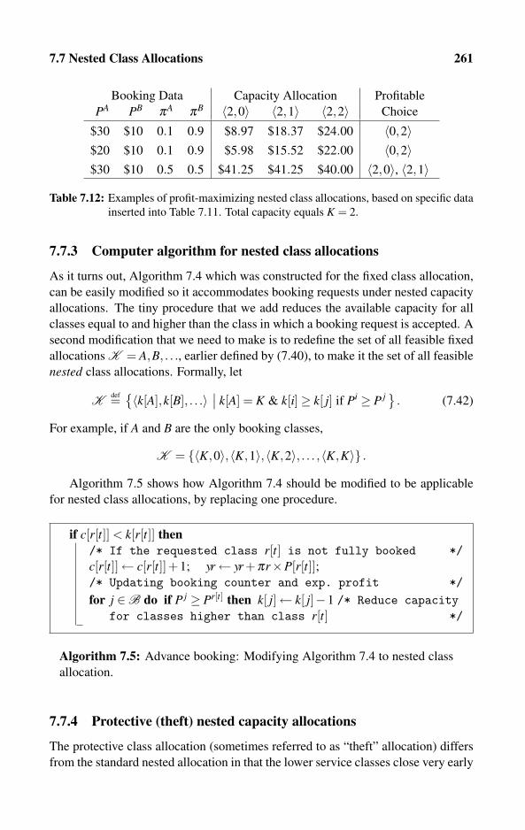
7.7 Nested Class Allocations 261
Booking Data Capacity Allocation Profitable
PA PB πA πB 〈2,0〉 〈2,1〉 〈2,2〉 Choice
$30 $10 0.1 0.9 $8.97 $18.37 $24.00 〈0,2〉$20 $10 0.1 0.9 $5.98 $15.52 $22.00 〈0,2〉$30 $10 0.5 0.5 $41.25 $41.25 $40.00 〈2,0〉, 〈2,1〉
Table 7.12: Examples of profit-maximizing nested class allocations, based on specific data
inserted into Table 7.11. Total capacity equals K = 2.
7.7.3 Computer algorithm for nested class allocations
As it turns out, Algorithm 7.4 which was constructed for the fixed class allocation,
can be easily modified so it accommodates booking requests under nested capacity
allocations. The tiny procedure that we add reduces the available capacity for all
classes equal to and higher than the class in which a booking request is accepted. A
second modification that we need to make is to redefine the set of all feasible fixed
allocations K = A,B, . . ., earlier defined by (7.40), to make it the set of all feasible
nested class allocations. Formally, let
Kdef={〈k[A],k[B], . . .〉 ∣∣ k[A] = K & k[i]≥ k[ j] if Pi ≥ P j} . (7.42)
For example, if A and B are the only booking classes,
K = {〈K,0〉,〈K,1〉,〈K,2〉, . . . ,〈K,K〉} .Algorithm 7.5 shows how Algorithm 7.4 should be modified to be applicable
for nested class allocations, by replacing one procedure.
if c[r[t]] < k[r[t]] then/* If the requested class r[t] is not fully booked */c[r[t]]← c[r[t]]+1; yr← yr +πr×P[r[t]];/* Updating booking counter and exp. profit */
for j ∈B do if P j ≥ Pr[t] then k[ j]← k[ j]−1 /* Reduce capacityfor classes higher than class r[t] */
Algorithm 7.5: Advance booking: Modifying Algorithm 7.4 to nested class
allocation.
7.7.4 Protective (theft) nested capacity allocations
The protective class allocation (sometimes referred to as “theft” allocation) differs
from the standard nested allocation in that the lower service classes close very early

262 Advance Booking
because a booking on any class reduces the capacity allocated for all classes. Recall
that under the standard nested class allocation, any booking reduces the allocated
capacity only in classes higher than (or equal to) the booked class.
Table 7.13 modifies Table 7.10 from standard to protective nested class alloca-
tion. The example assumes K = 100 units of capacity allocated among four book-
ing classes labeled A, B, C, and D. Table 7.13 demonstrates that under protective
t rt kt Booking Class (i): A B C D
Fixed allocation (Ki): 30 20 10 40
1 C 100 Protective nested allocation (Ki1): 100 70 50 40
2 D 99 Protective nested allocation (Ki2): 99 69 49 39
3 A 98 Protective nested allocation (Ki3): 98 68 48 38
4 B 97 Protective nested allocation (Ki4): 97 67 47 37
5 n/a 96 Protective nested allocation (Ki5): 96 66 46 36
Table 7.13: Protective (theft) nested class allocation of K = 100 units of capacity.
Note: rt denotes a realization of period t booking request.
nested capacity allocation, each time a booking request is accepted for any class,
the next period’s capacity allocation is reduced for all classes (as opposed to a re-
duction in equal or higher classes under the standard nested capacity allocation).
In view of this difference between the protective and standard capacity allocations,
Algorithm 7.5 can be easily modified to handle protective capacity allocation by re-
moving the condition “if P j ≥Pr[t]” from the last line. Under this modification, any
accepted booking request will result in a subsequent period’s reduction in capacity
allocated for all classes.
7.8 Exercises
1. Consider our first example given in Subsection 7.1.1 of a service provider who
allows only two booking periods and two fare classes. Suppose now that we
replace the potential consumer population given in Table 7.1 with the following
data:
Class (i) 0 A BProportion (π i) 0.4 0.1 0.5
Price/fare (Pi) $0 $40 $10
Table 7.14: Potential consumer population for Exercises 1 and 2.
(a) Using the same steps as in Subsection 7.1.1, derive the decision rules
d1(P1) and d2(P2) and the corresponding period 2 expected value of capacity
EV2(k2) by working backward from period t = 2 to period t = 1.
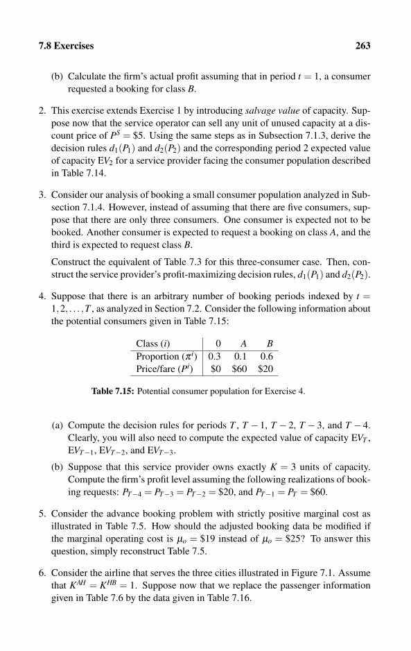
7.8 Exercises 263
(b) Calculate the firm’s actual profit assuming that in period t = 1, a consumer
requested a booking for class B.
2. This exercise extends Exercise 1 by introducing salvage value of capacity. Sup-
pose now that the service operator can sell any unit of unused capacity at a dis-
count price of PS = $5. Using the same steps as in Subsection 7.1.3, derive the
decision rules d1(P1) and d2(P2) and the corresponding period 2 expected value
of capacity EV2 for a service provider facing the consumer population described
in Table 7.14.
3. Consider our analysis of booking a small consumer population analyzed in Sub-
section 7.1.4. However, instead of assuming that there are five consumers, sup-
pose that there are only three consumers. One consumer is expected not to be
booked. Another consumer is expected to request a booking on class A, and the
third is expected to request class B.
Construct the equivalent of Table 7.3 for this three-consumer case. Then, con-
struct the service provider’s profit-maximizing decision rules, d1(P1) and d2(P2).
4. Suppose that there is an arbitrary number of booking periods indexed by t =1,2, . . . ,T , as analyzed in Section 7.2. Consider the following information about
the potential consumers given in Table 7.15:
Class (i) 0 A BProportion (π i) 0.3 0.1 0.6
Price/fare (Pi) $0 $60 $20
Table 7.15: Potential consumer population for Exercise 4.
(a) Compute the decision rules for periods T , T − 1, T − 2, T − 3, and T − 4.
Clearly, you will also need to compute the expected value of capacity EVT ,
EVT−1, EVT−2, and EVT−3.
(b) Suppose that this service provider owns exactly K = 3 units of capacity.
Compute the firm’s profit level assuming the following realizations of book-
ing requests: PT−4 = PT−3 = PT−2 = $20, and PT−1 = PT = $60.
5. Consider the advance booking problem with strictly positive marginal cost as
illustrated in Table 7.5. How should the adjusted booking data be modified if
the marginal operating cost is μo = $19 instead of μo = $25? To answer this
question, simply reconstruct Table 7.5.
6. Consider the airline that serves the three cities illustrated in Figure 7.1. Assume
that KAH = KHB = 1. Suppose now that we replace the passenger information
given in Table 7.6 by the data given in Table 7.16.

264 Advance Booking
Route (i) 0 AH HB ABProportion (π i) 0.1 0.1 0.1 0.7
Airfare (Pi) $0 $20 $30 $40
Table 7.16: Airline bookings: Passenger information for Exercise 6.
(a) Using the same steps as in Subsection 7.5.1, derive the decision rules d1(P1)and d2(P2) and the corresponding expected value of capacity EV1(kAH
1 ,kHB1 )
and EV2(kAH2 ,kHB
2 ) by working backward from booking period t = 2 to pe-
riod t = 1.
(b) Using the derived decision rules d1(P1) and d2(P2), compute the probability
that no capacity will be booked, that is, the probability that both flights will
take off with no passengers.
(c) Compute the probability that this airline will book a passenger on route AB.
(d) Compute the probability that this airline will book a passenger on route HB.
7. Consider the fixed class allocation model analyzed in Section 7.6. Compute the
profit-maximizing fixed class allocation 〈KA,KB〉 assuming that service classes
A and B are sold for PA = $20 and PB = $10 and are realized with probabilities
πA = 0.2 and πB = 0.8, respectively. Assume that the service provider allows
for three booking periods and there are a total of K = 2 units of capacity.
8. Solve the previous exercise assuming that there is only one unit of capacity
(K = 1). Hint: You must first modify Table 7.8 to incorporate the two possible
class allocations 〈KA,KB〉= 〈1,0〉 and 〈KA,KB〉= 〈0,1〉.9. Consider the nested class allocation analyzed in Section 7.7. Assuming the same
initial capacity allocation as in Table 7.10, construct a similar table showing
the capacity allocation in each booking period t = 1,2,3,4 assuming that the
realized sequence of booking requests is given by r1 = A, r2 = B, r3 = C, and
r4 = D.
10. Compute the profit-maximizing nested class allocation for the industry de-
scribed in Exercise 7.
11. Solve the previous exercise assuming that there is only one unit of capacity
(K = 1). Hint: You must first modify Table 7.11 to incorporate the two possible
nested class allocations: 〈1,0〉, and 〈1,1〉.
Chapter 8
Refund Strategies
8.1 Basic Definitions 2678.1.1 Survival probabilities, no-shows, and cancellations
8.1.2 Service provider’s cost structure
8.1.3 Seller’s strategies
8.2 Consumers, Preferences, and Seller’s Profit 2708.2.1 Preferences and profits under lump-sum refunds
8.2.2 Preferences and profits under proportional refunds
8.2.3 Multiple consumer types
8.3 Refund Policy under an Exogenously Given Price 2748.3.1 Lump-sum refunds under an exogenously given price
8.3.2 Proportional refunds under an exogenously given price
8.4 Simultaneous Price and Refund Policy Decisions 2808.4.1 Two consumer types
8.4.2 Multiple consumer types: A computer algorithm
8.5 Multiple Price and Refund Packages 2888.6 Refund Policy under Moral Hazard 290
8.6.1 Survival probability under moral hazard
8.6.2 Refund setting under an exogenously given price
8.7 Integrating Refunds within Advance Booking 2938.8 Exercises 294
Refunds are widely observed in almost all privately provided services and also to
some degree in retail industries. Refunds are heavily used by travel-related service
providers. Most noticeably, refunds are heavily used by airlines where cheaper tick-
ets allow for a very small refund (if any) on cancellations and no-shows, whereas
full-fare tickets are either fully refundable or are subject to low cancellation penalty
rates.
In Chapter 7, we analyze service providers who face consumers who value ad-
vance reservation systems because they enable them to guarantee that the service

266 Refund Strategies
will be available at the contracted delivery time. However, the drawback of the
advance reservation system, to both consumers and service providers, is that con-
sumers may either cancel their reservations or simply may not show up at the time
when the contracted service is scheduled to be delivered. This will leave some ca-
pacity unused, thereby resulting in a loss to service providers. Clearly, this loss
can be minimized if service providers do not provide any refund to consumers who
either cancel or do not show up.
In this chapter, we show how service providers can enhance their profit and
extract higher surplus from consumers by offering refunds to consumers who either
cancel their reservations or simply do not show up. For most parts of this chapter,
we will not distinguish between a cancellation and a no-show. However, for the
sake of completeness, the following definition clarifies the difference between these
two terms.
DEFINITION 8.1
We say that a consumer with a confirmed reservation cancels the reservation if the
consumer notifies the service provider some time before the service delivery time
that the reservation will not be used. In contrast, a confirmed consumer’s no-showoccurs when the consumer does not show up at the service delivery time, with no
prior notice.
Definition 8.1 is not without problems, as the precise meaning of “some time be-
fore” the service delivery time is not clear. For example, should five-minute noti-
fication by the consumer be considered as a cancellation? However, this difficulty
is overcome by having the service provider specify on each confirmed ticket the
precise time frame that would qualify as a cancellation time, usually under the
terms and conditions of a sold ticket. Moreover, service providers can create such
a distinction by simply offering consumers different refund levels depending on
whether the consumer cancels in advance (and how long in advance) and whether
the consumer does not show up at the service delivery time. Clearly, all these terms
and conditions must be clearly specified at the time when the service is contracted,
usually when the reservations are made, or a ticket is issued and paid for.
Consumers who make reservations for products and services differ in their
probability of showing up to collect the good or the service at the pre-agreed time
of delivery. Agencies and dealers that sell these goods and services can save on
unused capacity costs, generated by consumers’ cancellations and no-shows, by
varying the degree of refunds offered to consumers who cancel or do not show up.
In this chapter, we show how the introduction of refunds serves as a price discrimi-
nation technique by which service providers attract consumers who are more likely
to cancel their reservations. The resulting increase in consumer base increases the
total surplus extracted from consumers. In the absence of refunds, service providers
may be induced to set the price sufficiently high so consumers who are likely to
cancel will not book this service.

8.1 Basic Definitions 267
Why do consumers have different probabilities of showing up? The best way
to think about it is to observe airline passengers. Passengers can be divided into
business travelers and leisure travelers. Business travelers are most likely to cancel
or change their reservations because their travel arrangements depend on others’
schedules and business opportunities. In contrast, students can be sure of their time
of travel because they tend to travel during semester breaks and holidays that are
not subjected to last-minute changes. All this means is that students are more likely
to engage in an advance purchase of discounted nonrefundable tickets, whereas
business travelers are less likely to commit in advance, and therefore are more likely
to either purchase fully refundable tickets or to postpone their ticket purchase to the
last minute.
In the economics literature, there are a few papers analyzing the refundability
option as a means for segmenting the market or the demand. Most studies have fo-
cused on a single seller. Contributions by Gale and Holmes (1992, 1993) compare
a monopolist’s advance bookings with socially optimal ones. Gale (1993) analyzes
consumers who learn their preferences only after they are offered an advance pur-
chase option. Along this line, Miravete (1996) and more recently Courty and Li
(2000) further investigate how consumers who learn their valuation over time can
be screened via the introduction of refunds. Courty (2003) investigates resale and
rationing strategies of a monopoly that can sell early to uninformed consumers or
late to informed consumers. Dana (1998) also investigates market segmentation un-
der advance booking made by price-taking firms. Ringbom and Shy (2004) analyze
partial refunds set by price-taking firms. Ringbom and Shy (2005) analyzes refund
setting under price competition and service providers’ incentives to semicollude on
a joint industry-wide refund policy.
8.1 Basic Definitions
We now lay out the basic formulation of the refund models used throughout this
chapter. Section 8.1.1 explains consumers’ behavior under the possibility of no-
show. Section 8.1.2 defines three types of service/production costs and explains
how each type of cost is affected by consumers’ no-shows. Finally, Section 8.1.3
summarizes the type of sellers’ refund strategies analyzed in this chapter.
8.1.1 Survival probabilities, no-shows, and cancellations
Let π denote the probability that a consumer will show up and consume the service
at contracted delivery time. We call π the survival probability, or the show-up
probability, where 0 ≤ π ≤ 1. Therefore, the probability of a cancellation and a
no-show is 1−π . We make the following assumption:
268 Refund Strategies
ASSUMPTION 8.1
Consumers’ survival probabilities (probabilities of showing up) are constant and
are unaffected by the refund level offered on no-shows and cancellations.
Assumption 8.1 implies that consumers’ cancellation decisions are exogenously
given in the sense that consumers actually do not make the decision to cancel or not
to show up. Instead, cancellations are determined by some external circumstances.
Clearly, Assumption 8.1 is too strong as it applies mainly to business-oriented ser-
vices in which cancellations are caused by a loss of business opportunities (or a
gain of some alternative opportunities). However, in many service markets, there
is a large number of consumers who are more likely to cancel when promised large
refunds. In fact, the introduction of refunds may even induce more consumers
who know they are likely to cancel to book this service. Some of these consumers
will not even bother to book the service when sold under nonrefundable contracts.
When survival probabilities change with the refund policy, we say that consumers
exhibit moral hazard behavior. Refund policy under moral hazard will be analyzed
in Section 8.6.
Let p denote the price of this service, and assume that all consumers must pay
for the service when the reservation is made. Also, let r denote the refund level
offered to consumers upon cancellation or a no-show. We assume consumers are
immediately reimbursed in the sense that they are paid r with “no questions asked”
if they cancel or simply do not show up. The following definitions establish some
terminology regarding the use of refunds by service providers.
DEFINITION 8.2
A refund policy on cancellations and no-shows is said to consist of
(a) Lump-sum refunds if consumers receive a fixed amount $r, where 0≤ r ≤ p.
(b) Proportional or percentage refunds if refunds are expressed as the fraction
r of the prepaid booking price, where 0 ≤ r ≤ 1. In this case, the amount
refunded equals r× p.
(c) Fixed cancellation fees, if consumers are reimbursed the prepaid price less a
pre-agreed fixed cancellation fee cn, where 0≤ cn≤ p.
(d) Proportional cancellation fees, if consumers receive their money back less a
certain fraction cn (percentage) of the prepaid price. In this case, the cancella-
tion fee equals cn× p, where 0≤ cn≤ 1.
Clearly, Definition 8.2(a) is equivalent to Definition 8.2(c) simply because the seller
can set cn = p− r. Similarly, Definition 8.2(b) is equivalent to Definition 8.2(d)
because the seller is free to set cn = 1− r. For this reason, our analysis in this
chapter will focus on refunds, but the reader should bear in mind that all refunds
can be expressed in terms of cancellation fees (as we just did).
Observe that cancellation fees are commonly used in service sectors. However,
in the mail-order industry, retailers tend to use a different terminology, namely,
shipping and handling (s&h) charges, instead of cancellation or penalty fees. From

8.1 Basic Definitions 269
a technical viewpoint, both types of fees serve the same purpose, which is to limit
the amount of refund given to consumers who would like to cancel a service, or
simply return a product. Of course, s&h sounds better than cancellation fees, but
this terminology does not translate into any practical difference. For this reason, in
this chapter we do not analyze s&h charges separately from other refund types.
The following definition classifies three possible refund levels.
DEFINITION 8.3
We say that the payment for a booking of a service is
• fully refundable if r = p, or (r = 1 meaning 100%),• nonrefundable if r = 0, or (r = 0 meaning 0%),• partially refundable if 0 < r < p, (0 < r < 1, meaning less than 100%).
Definition 8.3 describes the types of refund levels analyzed in this chapter. Thus,
we rule out extreme situations in which sellers set refund levels exceeding the pre-
paid price, r > p, as in reality this kind of consumer “subsidy” generates extreme
moral hazard effects in which people book the service just for the sake of obtaining
refunds.
8.1.2 Service provider’s cost structure
We now discuss the service provider’s (production side) cost structure. The fixed
and sunk costs, denoted by φ , are borne by the service provider (the seller or the
producer) independent of the seller’s refund policy and consumers’ cancellation
probabilities, and may even be ignored for most parts of our analysis. However,
marginal costs, which constitute the cost of providing an additional unit of service,
are sensitive to consumers’ show-up probabilities in the following way:
DEFINITION 8.4
The cost of providing an additional unit of service is called
• Marginal operating cost, denoted by μo, if this cost is borne only when the
consumer actually shows up at the service delivery time.
• Marginal capacity cost, denoted by μk, if this cost is borne each time a con-
sumer books one unit of service.
The marginal capacity cost (or booking cost) is a direct consequence of our as-
sumption that overbooking is not allowed. Overbooking is examined in detail in
Chapter 9. This means that the service provider must secure exactly one unit of
capacity each time a booking is made.
To give some examples that would clarify the distinction between the two types
of marginal costs described by Definition 8.4, we discuss some travel-related indus-
tries. In the airline industry, the marginal operating cost can be viewed as the price
of onboard services provided to passengers, such as meals and entertainment. In
the hotel industry, the marginal operating cost consists of the cost of cleaning up the
270 Refund Strategies
room, changing and washing sheets and towels, electricity and water consumption,
and so on. In contrast, marginal capacity cost in the airline industry consists of the
cost of expanding seating capacity by one seat (which corresponds to a change in
aircraft size divided by the number of flights). In the hotel business, this cost could
be the cost of building an additional hotel room divided by 365 days, say.
Clearly, the capacity cost is much harder to estimate as it depends on the cost
of capital, which depends on the interest rate. In fact, we have already classified
these two types of marginal costs in Chapter 6 where we analyzed peak-load pricing
problems. As already mentioned in Section 7.1.3, the real difficulty in estimating
marginal capacity cost stems from the fact that some of this capital has salvage
value. That is, the cost of booking one additional unit of capacity heavily depends
on the alternative use of unused capital in a no-show event. Here, we basically
assume that there is no salvage value of capital, and even if there is, it is already
imbedded into the parameter μk.
8.1.3 Seller’s strategies
In this chapter, we demonstrate how to compute profit-maximizing prices and re-
fund levels when service providers face a variety of different consumer types. How-
ever, industries may differ in the degree of flexibility of setting price and refund
levels. For this reason, we will be conducting our analysis under three types of
pricing instruments:
Refund setting only: In this type of industry, prices are fixed either by the regulator
or by the manufacturer (as opposed to the provider). Our investigation then
focuses on finding the profit-maximizing refund policy for any exogenously
given price.
Refund and price setting: The service provider is free to set a booking package
consisting of a price and a refund policy.
Multiple price–refund packages: The service provider designs a “menu” of differ-
ent “packages,” thereby segmenting the market so that different types of con-
sumers may buy different packages, each containing a different refund–price
combination.
8.2 Consumers, Preferences, and Seller’s Profit
We now specify how consumers make a decision whether or not to book the service.
Each consumer values the service/product at $V . That is, V is a consumer’s maxi-
mum willingness to pay for the actual delivery of the service or the consumption of
the product (whichever applies). In other words, the consumer is willing to pay $Vconditional on actually showing up and actually consuming the service when the

8.2 Consumers, Preferences, and Seller’s Profit 271
service is delivered. Clearly, if full refunds are not offered, the willingness to pay
should be lower as the consumer takes into account the possibilities of no-shows
and cancellations.
8.2.1 Preferences and profits under lump-sum refunds
We assume that each consumer maximizes the expected net benefit given by
U(p,r) def=
{πV − p+(1−π)r if he or she chooses to book the service
U does not book this service.(8.1)
Equation 8.1 is commonly referred to as a consumer’s (expected) utility function.
The term πV is the expected net benefit from consuming the service, taking into
account that this benefit is realized with probability π . Because the price is prepaid,
the price p must be deducted. In contrast, a refund r is reimbursed to the consumer
only in a no-show event, which occurs with probability 1−π .
For example, suppose a consumer values the actual delivery of a certain service
by V = $10 and there is a probability of 50% that the consumer will cancel the
reservation. The service provider sets a price p = $6 that must be paid at the time
the booking is made. Table 8.1 demonstrates how booking decisions are affected
by varying the refund level r according to the utility function (8.1). Table 8.1 shows
that the service provider can turn a not-booking decision into a booking decision
by increasing the promised refund level even without changing the market price.
The threshold refund level r = $2 leaves the consumer indifferent between booking
and not booking. In such a case, we will always assume that the consumer chooses
to book, simply because the seller can always increase the refund by 1/c, thereby
making a booking decision generating a strictly positive utility.
π V πV p r (1−π)r U Decision
0.5 10 5 6 0 0.0 −1.0 Not book
0.5 10 5 6 1 0.5 −0.5 Not book
0.5 10 5 6 2 1.0 0.0 Book
0.5 10 5 6 3 1.5 0.5 Book
Table 8.1: Refunds and booking decisions made according to (8.1), assuming a threshold
utility level of U = 0.
The examples listed in Table 8.1 assume a threshold utility level given by U = 0.
The threshold utility level reflects the utility generated from using an alternative ser-
vice, and could generally take values that differ from U = 0, as shown in Exercise 1
at the end of this chapter. The threshold utility level is often called “reservation util-
ity” by academic economists; however, we avoid using this terminology to prevent
confusion with booking (making reservations) decisions analyzed throughout this
book.

272 Refund Strategies
We end our discussion of the consumer side with a graphical visualization of
booking decisions under refunds. Extracting the refund level r from πV − p+(1−π)r = U , where U is the threshold utility level, obtains
r =U
1−π+
p−πV1−π
. (8.2)
In particular, for the specific utility function (8.1) where U = 0,
r =p−πV1−π
, (8.3)
which is plotted in Figure 8.1. The area above the dashed line represents refund
levels exceeding the price, which are ruled out by assumption. Under the dashed
line, all booking offers with a sufficiently high refund and/or a sufficiently low
price will be accepted by the consumer. Clearly, holding r constant and increasing
p beyond a certain level would change the consumer’s decision to not book the
service. Finally, Figure 8.1 shows that even with a full refund, the price must not
exceed p = r = V to induce the consumer to book this service. Note that p = r = Vis also the unique solution to (8.3) after substituting p = r.
�r
0
���������������
(8.3) r = p
r > p(ruled out)
B NB
−πV1−π
V�
V
p
r < 0(ruled out)
Figure 8.1: Lump-sum refund: Book (B) and no-book (NB) utility decision.
We now define the profit function of a service provider. Suppose that n con-
sumers decide to book the service and prepay the given price of p. Let r be the
agreed upon refund level on a no-show. The expected profit of this service provider
is given by
y def= n(p−μk)−πnμo− (1−π)r−φ . (8.4)

8.2 Consumers, Preferences, and Seller’s Profit 273
The first term in (8.4) constitutes the sales revenue net of the cost of reserving nunits of capacity. The second term is the expected operating cost that depends on
the number of actual shows πn. The third term is the expected cost associated
with paying refunds to consumers who cancel. The last term is the fixed cost φ ,
which generally does not affect any price decision but should be considered when
evaluating the long-run profitability of the firm. For this reason, in a few examples
we simply set φ = 0.
8.2.2 Preferences and profits under proportional refunds
Proportional (percentage) refunds are analyzed only in Section 8.3.2, so readers
who wish to skip this section as well as Section 8.3.2 can do it without any con-
sequences on the understanding of all other sections in this chapter. Suppose now
that instead of giving a lump-sum refund of $r, the service provider commits to a
refund that is proportional to the prepaid booking price. So, we now let r be a frac-
tion 0≤ r≤ 1 of the price given to consumers who cancel or do not show. Thus, the
refunded amount now becomes r× p. Under proportional refund, the consumers’
expected utility function (8.1) becomes
U(p,r) def=
{πV − p+(1−π)rp if they choose to book the service
0 not book this service.(8.5)
We now provide a graphical visualization of booking decisions under propor-
tional refunds. Extracting the refund rate r from πV − p +(1−π)rp = 0 where 0
is the threshold utility level obtains
r =p−πV
(1−π)p, (8.6)
which is plotted in Figure 8.2. Similar to Figure 8.1, any combination of price and
refund levels above the curve will be accepted and booked by consumers. Any
combination below the curve will be rejected as the booking yields an expected
utility below the threshold level. Also, Figure 8.2 clearly shows that as long as
the service provider charges a price below the expected consumers’ benefit πV ,
consumers will book this service even if no refund is given.
8.2.3 Multiple consumer types
So far, we characterized the preferences of a single individual who has a basic
valuation of V for the service, and a survival probability π . We now extend the
model to multiple consumer types. Let there be M consumer types, indexed by
� = 1,2, . . . ,M. When there are only two types, we sometimes index types by
� = H,L to indicate high and low survival probabilities. There are N� consumers of
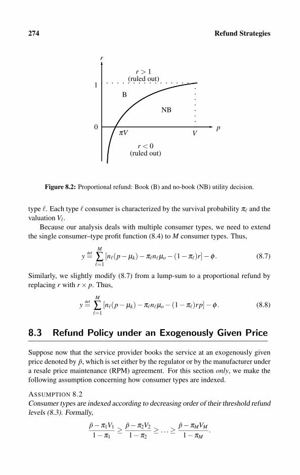
274 Refund Strategies
0 � p
r < 0(ruled out)
NB
B
1
VπV
r > 1(ruled out)
�r
Figure 8.2: Proportional refund: Book (B) and no-book (NB) utility decision.
type �. Each type � consumer is characterized by the survival probability π� and the
valuation V�.
Because our analysis deals with multiple consumer types, we need to extend
the single consumer–type profit function (8.4) to M consumer types. Thus,
y def=M
∑�=1
[n�(p−μk)−π�n�μo− (1−π�)r]−φ . (8.7)
Similarly, we slightly modify (8.7) from a lump-sum to a proportional refund by
replacing r with r× p. Thus,
y def=M
∑�=1
[n�(p−μk)−π�n�μo− (1−π�)rp]−φ . (8.8)
8.3 Refund Policy under an Exogenously Given Price
Suppose now that the service provider books the service at an exogenously given
price denoted by p, which is set either by the regulator or by the manufacturer under
a resale price maintenance (RPM) agreement. For this section only, we make the
following assumption concerning how consumer types are indexed.
ASSUMPTION 8.2
Consumer types are indexed according to decreasing order of their threshold refund
levels (8.3). Formally,
p−π1V1
1−π1≥ p−π2V2
1−π2≥ . . .≥ p−πMVM
1−πM.

8.3 Refund Policy under an Exogenously Given Price 275
It is very important to stress that Assumption 8.2 is made with no loss of gener-
ality whatsoever as it merely requires a re-indexation of consumer types. In other
words, Assumption 8.2 is not really an assumption as it only guides us in labeling
consumer types to facilitate the profit-maximization algorithms developed in this
section.
8.3.1 Lump-sum refunds under an exogenously given price
Under a fixed booking price, this section computes the lump-sum refund level 0≤r ≤ p that maximizes the seller’s profit.
Two consumer types: An example
Consider a single service provider facing two types of consumers, labeled type � =H (high survival probability) and type � = L (low survival probability), as described
by Table 8.2. All consumers are assumed to make their book–not-book decisions as
to maximize the utility function defined by (8.1). In this simple example, there are
500 type H potential consumers with a survival probability of πH = 0.8, and a basic
valuation for this service given by VH = $10. Similarly, there are 800 type L con-
sumers with a survival probability of πL = 0.5, with a basic valuation of VL = $10.
Thus, the first four columns of Table 8.2 constitute the exogenous data, whereas the
remaining three columns are simple computations of expected value of the service,
expected number of show-ups of each group, and expected number of no-shows.
Consumers Some Computations
� N� π� V� π�V� π�N� (1−π�)N�
H 500 0.8 10 8 400 100
L 800 0.5 10 5 400 400
Seller’s Cost
μo μk φ2 1 1000
Table 8.2: Two-consumer type example.
In what follows, we analyze the possible profit-maximizing refund settings of
the service provider with the cost structure given in Table 8.2. Suppose the service
price is fixed at the level p = $6 and the service provider cannot change this price.
Thus, the only strategic variable available to this seller is to set a uniform refund
policy for all consumers, r, where 0≤ r ≤ p. We analyze three refund policies: no
refund (NR), where r = 0, full refund (FR), where r = p = 6, and a partial refund
(PR), where 0 < r < p.
Under no refund, type L consumers do not book the service because if they
do, by (8.1) their utility level would be UL = 0.5× 10− 6 < 0. However, type Hconsumers book the service because UH = 0.8×10⁻⁶ > 0. Substituting p = 6 and
the data from Table 8.2 into (8.4) yields the seller’s profit level
yNR = 500(6−1)−0.8×500×2− (1−0.8)0−1000 = 700. (8.9)

276 Refund Strategies
Now suppose the seller provides a full refund so that r = 6. Under this policy,
type L consumers book this service because UL = 0.5×10⁻⁶+(1−0.5)6 = 2 > 0.
Type H consumers also book this service because UH = 0.8×10⁻⁶+(1−0.2)6 >0. Substituting r = p = 6 and the data from Table 8.2 into (8.7) yields the seller’s
profit level
yFR = (500+800)(6−1)− (0.8×500+0.5×800)2− (0.2×500+0.5×800)6−1000 = 900. (8.10)
Comparing (8.10) with (8.9) shows that in this example giving a full refund
yields a higher profit than giving no refund at all. This is not very surprising con-
sidering the fact that because the price is fixed, giving refunds substitutes for a price
reduction, which is needed to attract the 800 type L consumers to book this service.
Next, we ask whether providing only a partial refund can further increase the
seller’s profit beyond yFR = 900. The answer to this question depends on whether
a reduction in the level below r = 6 will induce some consumers not to book the
service. Thus, we seek to find a refund level r that solves UL = 0.5×10⁻⁶+(1−0.5)r ≥ 0, yielding r ≤ 2. Hence, a refund level of r = 2 is the lowest refund level
that would still induce type L consumers to book the service. Notice that r = 2
implies that UH = 0.8×10− 6 +(1− 0.2)2 > 0, hence, type H consumers would
also find it beneficial to book this service. Substituting r = 2, p = 6, and the data
from Table 8.2 into (8.7) yields the seller’s profit level
yPR = (500+800)(6−1)− (0.8×500+0.5×800)2
− (0.2×500+0.5×800)2−1000 = 2900 > yFR > yNR. (8.11)
It should be pointed out that a partial refund not only increases profit over a full
refund, it also has the advantage of reducing moral hazard effects by providing
lower incentives for cancellations and no-shows. Moral hazard effects were ruled
out by our assumption of fixed show-up probabilities. This assumption is relaxed
in Section 8.6 below.
Multiple consumer types: A general algorithm
The two-consumer type analysis conducted so far turned out to be very useful for
learning the intuition behind the technique for searching for the profit-maximizing
refund level. The above two-consumer type analysis also taught us that we must
always take into consideration that the seller may not find it profitable to serve the
entire market. That is, under some circumstances, which were carefully character-
ized in the above analysis, the seller may want to reduce the refund level to exclude
consumers with either a low expected valuation and/or a low survival probability.
We now extend the model to M consumer types, which we have already care-
fully described in Section 8.2.3. Recalling (8.3), given a booking price p, a type �

8.3 Refund Policy under an Exogenously Given Price 277
consumer will book the service only if
r ≥max
{0,
p−π�V�
1−π�
}, for each consumer type � = 1,2, . . . ,M, (8.12)
that is, only if the refund level exceeds the type-specific threshold level described
by (8.12). We are now ready to state the complete algorithm for setting refunds,
taking into account the possibility of exclusion of some consumer types.
Step I: Check and verify that your data satisfy Assumption 8.2 so that
p−π1V1
1−π1≥ p−π2V2
1−π2≥ . . .≥ p−πMVM
1−πM.
Step II: Using the threshold refund levels (8.12), set the highest refund level r that
would still induce all consumer types to book this service. Substitute r into
the profit function (8.7), and record the resulting profit level as yM (to indicate
that all the M consumer types are served).
Step III: Delete the last type from the problem and set the highest refund level that
would still induce types 1, . . . ,M− 1 to book the service. Record the profit
level as yM−1.
Step IV: Repeat Step III (each time deleting the last type from the problem), and
record the resulting profit levels as yM−2, yM−3 until y1.
Step V: Pick the profit-maximizing price–refund pair by comparing the profit lev-
els y1,y2, . . . ,yM.
We now implement the above algorithm using the example described in Ta-
ble 8.3, assuming an exogenously given price of p = 6. The fifth column of Ta-
ble 8.3 confirms Assumption 8.2, thus Step I of the above algorithm is now com-
pleted.
Consumers Some Computations
� N� π� V�p−π�V�1−π�
π�N� (1−π�)N�
1 500 0.8 8 −2 400 100
2 500 0.5 10 2 250 250
3 300 0.5 8 4 150 150
Seller’s Cost
μo μk φ2 1 1000
Table 8.3: Three consumer type example.
Moving on to Step II, substituting π3 = 0.5 and V3 = 8 into (8.12) yields r = 4.
Substituting all values into the profit (8.7) obtains y3 = 1900.
Moving on to Step III, substituting π2 = 0.5 and V2 = 10 into (8.12) yields
r = 2. Substituting all values into the profit (8.7) obtains y2 = 2000.

278 Refund Strategies
Moving on to Step IV, substituting π1 = 0.8 and V1 = 8 into (8.12) yields r =max{0,−2} = 0. Substituting all values into the profit (8.7) obtains y1 = 700.
Hence, the profit-maximizing refund level is r = 2. When this level of refund is
offered to consumers, only consumer types 1 and 2 book this service.
Multiple consumer types: A computer algorithm
The computer algorithm described by Algorithm 8.1 should first input the param-
eters describing consumer types: M (number of consumer types), N[�], π[�], and
V [�] (each array of a dimension M). The exact nature of these arrays (such as, Real,
Integer) are specified in Table 1.4. The program should also input three cost param-
eters, μo, μk, and φ . Finally, the program should input the price p. In addition, the
program should include some trivial loops to ensure that there are no out-of-range
(or negative) parameters and that the ranking given by Assumption 8.2 is obeyed.
At this stage, some sorting may be needed to establish the required ranking. Results
over the M loops are written onto the refund and profit M + 1 dimensional arrays
r[i] and y[i], where the final (profit-maximizing) result will be written as r[0] and
y[0], respectively. yy[�] will record the profit made from type � only (to be added
later to the combined profit made from all consumer types who actually book the
service).
for � = 1 to M dor[�]← p−π[�]×V [�]
1−π[�] ; /* Types’ threshold refund levels */
if r[�] < 0 then r[�]← 0; /* Ensure nonnegative value */yy[�]← N[�](p−μk)−π[�]×N[�]×μo− (1−π[�])N[�]× r[�] ;
/* Compute the profit made from type � only */
for i = M downto 1 do/* Bottom-to-top type exclusions: Profits */for � = 1 to i do y[i]← y[i]+ yy[�];/* Add up profits from all non-excluded types */y[i]← y[i]−φ ; /* Subtract fixed cost */
for � = 1 to M do/* Maximize profit. Write results onto y[0], r[0], � */
if y[0] < y[�] then y[0]← y[�]; r[0]← r[�]; �← �;
writeln (“The profit-maximizing refund level is ”, r[0],“.”);
writeln (“The resulting profit level is ”, y[0], “.”);
write (“The following types will book the service: ”);
for � = � to M do write (�, “,”);
Algorithm 8.1: Refund setting under an exogenously given price.

8.3 Refund Policy under an Exogenously Given Price 279
8.3.2 Proportional refunds under an exogenously given price
Let us assume again that the service provider books the service for an exogenously
given price denoted by p, which is set either by the regulator or by the manufac-
turer under an RPM agreement. Under this restriction, this section computes the
proportional (percentage) refund rate 0≤ r ≤ 1 that maximizes the seller’s profit.
As it turns out, as long as the service price is exogenously given, the analysis of
proportional refunds is not much different from the analysis of lump-sum refunds
described in Section 8.3.1, except that we use the utility function (8.5) instead of
(8.1), and the profit function (8.8) instead of (8.7).
Two-consumer type: An example
Consider again the consumers’ and the seller’s cost structure exhibited in Table 8.2,
and suppose that the booking price also remains p = 6. Because the profit levels
under no refund and full refund given by (8.9) and (8.10) remain the same, we
will not recompute these profit levels. Instead, we proceed directly to our main
question, which is finding the profit-maximizing refund rate. Thus, we seek to find
a refund rate r that solves
UL = 0.5×10⁻⁶+(1−0.5)r×6≥ 0, yielding r ≤ 1
3.
Hence, a refund rate r = 1/3 is the lowest refund level that would still induce
type L consumers to book the service. Notice that r = 1/3 implies that UH =0.8× 10− 6 + (1− 0.2)(1/3)6 > 0, hence type H consumers would also find it
beneficial to book this service. Substituting r = 1/3, p = 6, and the data from
Table 8.2 into (8.8) yields the seller’s profit level,
yPR = (500+800)(6−1)− (0.8×500+0.5×800)2
− (0.2×500+0.5×800)1
36−1000 = 2900 > yFR > yNR. (8.13)
As expected, the profit level (8.13) equals the profit level under the optimal lump-
sum refund rate given by (8.11). In fact, this computation was not really needed
given our computations in Section 8.3.1 that showed that a lump-sum refund of
$2 is profit maximizing. That is, we only need to extract r from r× p = 6r = 2,
yielding the refund rate r = 1/3≈ 33.3%.
Multiple consumer types: A general algorithm
We now extend the model to M consumer types, which we have already carefully
described in Section 8.2.3. Recalling (8.6), given a booking price p, a type � con-
sumer will book the service only if
r ≥max
{0,
p−πV(1−π)p
}for each consumer type � = 1,2, . . . ,M, (8.14)

280 Refund Strategies
that is, only if the refund level exceeds the type-specific threshold level described
by (8.14). Because (8.14) equals the lump-sum threshold (8.12) divided by the
price p, there is no need to restate the complete algorithm for setting the profit-
maximizing refund level, developed earlier in Section 8.3.1. In fact, only Step II
should be slightly modified as follows:
Step II: Using the threshold refund levels (8.14), set the highest refund rate r that
would still induce all consumer types to book this service. Substitute r into
the profit function (8.8), and record the resulting profit level as yM (to indicate
that all the M types are served).
All other steps remain unchanged. Therefore, we can conclude that the profit-
maximizing refund rate for a seller facing the consumers described by Table 8.3 is
r = 2/ p = 2/6 = 33.33%.
8.4 Simultaneous Price and Refund Policy Decisions
Suppose now that the service provider simultaneously sets the booking price p and
the refund policy. We confined our analysis to lump-sum refunds only. Therefore,
recalling (8.1), each type � consumer makes a book–not-book decision to maximize
a utility function given by
U(p,r) def=
{π�V�− p+(1−π�)r if he or she books the service
0 does not book this service.(8.15)
On the supply side of this market, recalling (8.7), the service provider chooses a
single pair of price and refund levels (p,r) to solve
maxp,r
y def=M
∑�=1
[n�(p−μk)−π�n�μo− (1−π�)r]−φ . (8.16)
Thus, n� = N� if type � consumers book the service, whereas n� = 0 if they choose
not to book. It should be emphasized that in this section the seller chooses one
and only one price–refund pair (p,r) that is offered to all consumers, who then
each makes a book–not-book decision. The reader is referred to Section 8.5, which
analyzes the offering of multiple price–refund packages.
8.4.1 Two consumer types
Suppose there are two types of consumers indexed by � = H,L. There are N� con-
sumers with survival probability π� whose valuation for the service is V�, for each
type � = H,L.
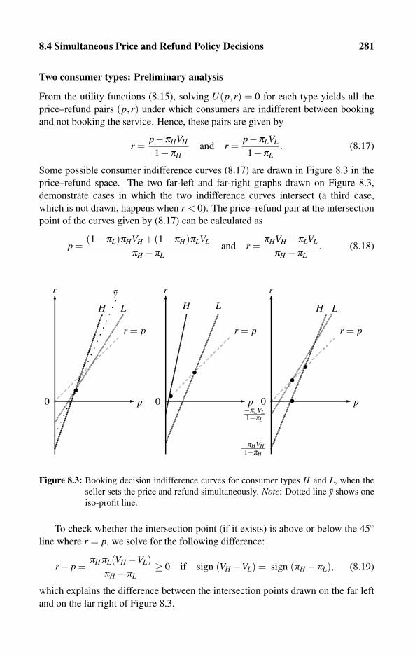
8.4 Simultaneous Price and Refund Policy Decisions 281
Two consumer types: Preliminary analysis
From the utility functions (8.15), solving U(p,r) = 0 for each type yields all the
price–refund pairs (p,r) under which consumers are indifferent between booking
and not booking the service. Hence, these pairs are given by
r =p−πHVH
1−πHand r =
p−πLVL
1−πL. (8.17)
Some possible consumer indifference curves (8.17) are drawn in Figure 8.3 in the
price–refund space. The two far-left and far-right graphs drawn on Figure 8.3,
demonstrate cases in which the two indifference curves intersect (a third case,
which is not drawn, happens when r < 0). The price–refund pair at the intersection
point of the curves given by (8.17) can be calculated as
p =(1−πL)πHVH +(1−πH)πLVL
πH −πLand r =
πHVH −πLVL
πH −πL. (8.18)
�r
0 �
r = p
p
�r
0 �
r = p
p
�r
0 �
r = p
p•
•
H L H L
y
−πHVH1−πH
−πLVL1−πL
•
•
LH
•
•
Figure 8.3: Booking decision indifference curves for consumer types H and L, when the
seller sets the price and refund simultaneously. Note: Dotted line y shows one
iso-profit line.
To check whether the intersection point (if it exists) is above or below the 45◦
line where r = p, we solve for the following difference:
r− p =πHπL(VH −VL)
πH −πL≥ 0 if sign (VH −VL) = sign (πH −πL), (8.19)
which explains the difference between the intersection points drawn on the far left
and on the far right of Figure 8.3.

282 Refund Strategies
Turning to the seller side, the set of iso-profit lines in the price–refund space
can be derived directly from (8.16) by setting y = y to obtain
r =(NH +NL)p+ y+NH(μk +πH μo)+NL(μk +πLμo)
NH(1−πH)+NL(1−πL), (8.20)
which is drawn as a dotted line in Figure 8.3(left) and marked by y to indicate a
fixed service output level. It is important to note that the iso-profit lines (8.20) are
valid only if both consumer types actually book this service. Under this restriction,
Figure 8.3 shows that the slope of the iso-profit line falls between the slopes of the
types’ indifference curves given by (8.17). To confirm that this is indeed the case,
the slopes of (8.17) and (8.20) are ranked as follows:
1
1−πH>
NH +NL
NH(1−πH)+NL(1−πL)>
1
1−πL, (8.21)
for the case in which πH > πL. This ranking confirms the slopes depicted in Fig-
ure 8.3(left). Note that if πH < πL, we need only the reverse the slopes given by
(8.21), but the iso-profit line remains between them.
We must also stress that the ranking of the slopes given by (8.21) is valid only if
both consumer types book this service. To demonstrate this point, we now compute
the slope of the iso-profit line assuming that only one type � books the service.
Then, the profit function (8.16), ignoring the summation sign, implies that
r =N�(p−μk−π�μo)− y
N�(1−π�), which is sloped
1
1−π�, (8.22)
for type � = H or type � = L, but not both. Hence, when only one consumer type is
served, the slope of the iso-profit line coincides with the slope of the type’s indiffer-
ence curve. We can conclude that when only one consumer type is served, there are
infinitely many profit-maximizing price–refund pairs because the iso-profit lines
coincide with the indifference curves of the type that is being served.
Two consumer types: The algorithm
We now provide the general algorithm for finding the seller’s profit-maximizing
price and refund levels. First, observe that in Figure 8.3, any movement above
and to the left of an indifference curve increases consumers’ utility because such a
movement is associated with a lower price and a higher refund. Second, a move-
ment in the opposite direction, that is, below and to the right of an iso-profit line,
increases the seller’s profit because the price increases whereas the refund level
declines. Thus, graphically speaking and using Figure 8.3, the seller’s profit-
maximization problem is to find the price–refund combination that is as far to the
right as possible subject to having this combination lying on the relevant indiffer-
ence curves and the restriction that r ≤ p (refunds cannot exceed the booking price
by assumption). This suggests the following algorithm for the seller’s selection of
the price–refund pair, given that there are only two consumer types.
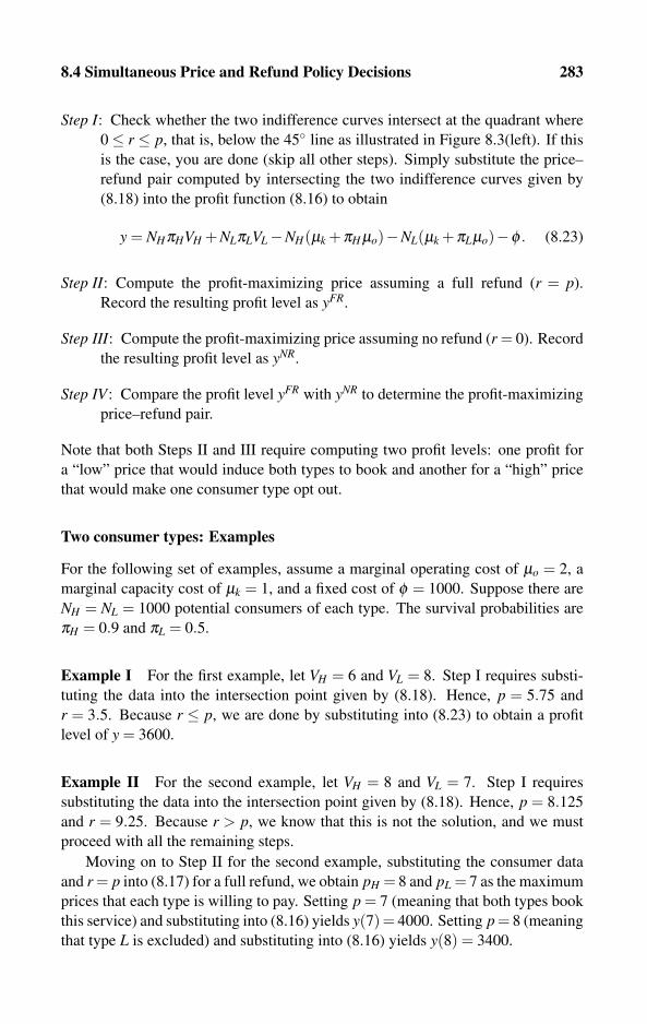
8.4 Simultaneous Price and Refund Policy Decisions 283
Step I: Check whether the two indifference curves intersect at the quadrant where
0≤ r ≤ p, that is, below the 45◦ line as illustrated in Figure 8.3(left). If this
is the case, you are done (skip all other steps). Simply substitute the price–
refund pair computed by intersecting the two indifference curves given by
(8.18) into the profit function (8.16) to obtain
y = NHπHVH +NLπLVL−NH(μk +πH μo)−NL(μk +πLμo)−φ . (8.23)
Step II: Compute the profit-maximizing price assuming a full refund (r = p).
Record the resulting profit level as yFR.
Step III: Compute the profit-maximizing price assuming no refund (r = 0). Record
the resulting profit level as yNR.
Step IV: Compare the profit level yFR with yNR to determine the profit-maximizing
price–refund pair.
Note that both Steps II and III require computing two profit levels: one profit for
a “low” price that would induce both types to book and another for a “high” price
that would make one consumer type opt out.
Two consumer types: Examples
For the following set of examples, assume a marginal operating cost of μo = 2, a
marginal capacity cost of μk = 1, and a fixed cost of φ = 1000. Suppose there are
NH = NL = 1000 potential consumers of each type. The survival probabilities are
πH = 0.9 and πL = 0.5.
Example I For the first example, let VH = 6 and VL = 8. Step I requires substi-
tuting the data into the intersection point given by (8.18). Hence, p = 5.75 and
r = 3.5. Because r ≤ p, we are done by substituting into (8.23) to obtain a profit
level of y = 3600.
Example II For the second example, let VH = 8 and VL = 7. Step I requires
substituting the data into the intersection point given by (8.18). Hence, p = 8.125
and r = 9.25. Because r > p, we know that this is not the solution, and we must
proceed with all the remaining steps.
Moving on to Step II for the second example, substituting the consumer data
and r = p into (8.17) for a full refund, we obtain pH = 8 and pL = 7 as the maximum
prices that each type is willing to pay. Setting p = 7 (meaning that both types book
this service) and substituting into (8.16) yields y(7) = 4000. Setting p = 8 (meaning
that type L is excluded) and substituting into (8.16) yields y(8) = 3400.

284 Refund Strategies
Moving on to Step III for the second example, substituting the consumer data
and r = 0 into (8.17) for no refund, we obtain pH = 7.2 and pL = 3.5 as the max-
imum prices that each type is willing to pay. Setting p = 3.5 (meaning that both
types book this service) and substituting into (8.16) yields y(3.5) = 1200. Set-
ting p = 8 (meaning that type L is excluded) and substituting into (8.16) yields
y(7.2) = 3400.
Comparing the four profit levels from Steps II and III clearly shows that the
solution to the second example is to provide a full refund and to set p = r = 7,
thereby serving all consumer types and earning a profit of yFR = 4000.
Example III Suppose that VH = 8 and VL = 6. Step I requires substituting the
data into the intersection point given by (8.18). Hence, p = 8.25 and r = 10.5.
Because r > p, we know that this is not the solution, and we must proceed with all
the remaining steps.
Moving on to Step II for the third example, substituting the consumer data and
r = p into (8.17) for a full refund, we obtain pH = 8 and pL = 6 as the maximum
prices that each type is willing to pay. Setting p = 6 (meaning that both types
book this service) and substituting into (8.16) yields y(6) = 2600. Setting p = 8
(meaning that type L is excluded) and substituting into (8.16) yields y(8) = 3400.
Moving on to Step III for the third example, substituting the consumer data and
r = 0 into (8.17) for no refund, we obtain pH = 7.2 and pL = 3 as the maximum
prices that each type is willing to pay. Setting p = 3 (meaning that both types book
this service), and substituting into (8.16) yields y(3) = 200. Setting p = 8 (meaning
that type L is excluded) and substituting into (8.16) yields y(7.2) = 3400.
Comparing the four profit levels from Steps II and III clearly shows that any
solution to the third example involves serving only type H consumers, thereby
earning a profit of yFR(8) = yNR(7.2) = 3400.
8.4.2 Multiple consumer types: A computer algorithm
The two-consumer type analysis conducted so far in this section turns out to be
very useful for learning the intuition behind the simultaneous setting of profit-
maximizing price and refund levels. The two-consumer type analysis is also very
useful in demonstrating the extreme linear nature of our refund models, which
stems from having to maximize a linear profit function subject to several linear
constraints. The constraints are linear because they reflect consumers’ indifference
curves, which are derived from linear expected utility functions.
The two-consumer type analysis has also taught us that we must always take
into consideration that the seller may not find it profitable to serve the entire mar-
ket. That is, under some circumstances, which were carefully characterized in the
above analysis, the seller may want to increase the booking price and/or reduce the

8.4 Simultaneous Price and Refund Policy Decisions 285
refund level, which may exclude consumers with either a low valuation and/or a
low survival probability.
From a practical point of view, because all personal computers and even many
online JavaScript Web pages are equipped with algorithms for solving linear pro-
gramming problems, we gear this section toward developing an algorithm that uses
built-in linear programming algorithms. We construct such an algorithm, taking
into account the possibilities that the profit-maximizing price and refund level may
at times be sufficiently high as to exclude consumers with either low valuations or
low survival probabilities.
Deriving the general algorithm
The purpose of this algorithm is to choose a pair (p,r) to maximize the profit func-
tion (8.16) subject to the following list of constraints:
r ≥ 0, p≥ 0, r ≤ p, and r ≥ p−π�V�
1−π�
for each consumer type � = 1,2, . . . ,M. (8.24)
This profit-maximization problem has M +3 linear constraints and two variables, pand r. The last term in (8.24) is derived from type �’s utility function (8.15). Each
constraint indicates that the refund level r should be sufficiently high relative to the
price p to induce a consumer type � to book this service.
Clearly, this problem can be solved by any elementary linear programming
software using, say, the Simplex method. Unfortunately, solving the above problem
may not yield the right solution because, as we have learned from the two consumer
type examples, in some cases the service provider may find it profitable to raise the
price or lower the refund level, which may exclude some consumer types from
booking the service. Thus, the reader should not rush to conclude that a single
linear programming algorithm always delivers the final solution. For example, let
us reformulate our last (third) example where VH = 8 and VL = 6. Substituting all
the numerical parameters, the problem reduces to
maxp,r
y = 200(10p−3r−24)−1000 subject to r ≥ 0, p≥ 0, r ≤ p,
r ≥ 2(5p−36), and r ≥ 2(p−3). (8.25)
The reader who substitutes (8.25) into linear programming software will obtain the
solution p = r = 6 and y = 2600, which is incorrect, as the third example analyzed
above shows.
In view of the above example, we now state an algorithm for tackling the possi-
bility of exclusion of some consumer types. The underlying principle of this algo-
rithm is simple. We let the computer determine the profit-maximizing price–refund
pair for all possible subsets of the set containing the M consumer types. Then, the
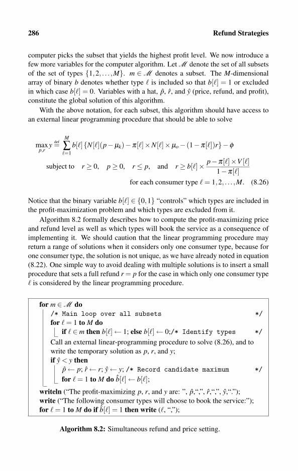
286 Refund Strategies
computer picks the subset that yields the highest profit level. We now introduce a
few more variables for the computer algorithm. Let M denote the set of all subsets
of the set of types {1,2, . . . ,M}. m ∈M denotes a subset. The M-dimensional
array of binary b denotes whether type � is included so that b[�] = 1 or excluded
in which case b[�] = 0. Variables with a hat, p, r, and y (price, refund, and profit),
constitute the global solution of this algorithm.
With the above notation, for each subset, this algorithm should have access to
an external linear programming procedure that should be able to solve
maxp,r
y def=M
∑�=1
b[�]{N[�](p−μk)−π[�]×N[�]×μo− (1−π[�])r}−φ
subject to r ≥ 0, p≥ 0, r ≤ p, and r ≥ b[�]× p−π[�]×V [�]1−π[�]
for each consumer type � = 1,2, . . . ,M. (8.26)
Notice that the binary variable b[�] ∈ {0,1} “controls” which types are included in
the profit-maximization problem and which types are excluded from it.
Algorithm 8.2 formally describes how to compute the profit-maximizing price
and refund level as well as which types will book the service as a consequence of
implementing it. We should caution that the linear programming procedure may
return a range of solutions when it considers only one consumer type, because for
one consumer type, the solution is not unique, as we have already noted in equation
(8.22). One simple way to avoid dealing with multiple solutions is to insert a small
procedure that sets a full refund r = p for the case in which only one consumer type
� is considered by the linear programming procedure.
for m ∈M do/* Main loop over all subsets */for � = 1 to M do
if � ∈ m then b[�]← 1; else b[�]← 0;/* Identify types */
Call an external linear-programming procedure to solve (8.26), and to
write the temporary solution as p, r, and y;
if y < y thenp← p; r← r; y← y; /* Record candidate maximum */
for � = 1 to M do b[�]← b[�];
writeln (“The profit-maximizing p, r, and y are: ”, p,“,”, r,“,”, y,“.”);
write (“The following consumer types will choose to book the service:”);
for � = 1 to M do if b[�] = 1 then write (�, “,”);
Algorithm 8.2: Simultaneous refund and price setting.
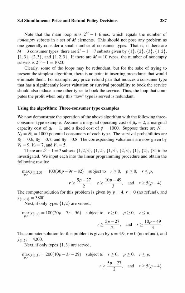
8.4 Simultaneous Price and Refund Policy Decisions 287
Note that the main loop runs 2M − 1 times, which equals the number of
nonempty subsets in a set of M elements. This should not pose any problem as
one generally consider a small number of consumer types. That is, if there are
M = 3 consumer types, there are 23−1 = 7 subsets given by {1}, {2}, {3}, {1,2},{1,3}, {2,3}, and {1,2,3}. If there are M = 10 types, the number of nonempty
subsets is 210−1 = 1023.
Clearly, some of the loops may be redundant, but for the sake of trying to
present the simplest algorithm, there is no point in inserting procedures that would
eliminate them. For example, any price–refund pair that induces a consumer type
that has a significantly lower valuation or survival probability to book the service
should also induce some other types to book the service. Thus, the loop that com-
putes the profit when only this “low” type is served is redundant.
Using the algorithm: Three-consumer type examples
We now demonstrate the operation of the above algorithm with the following three-
consumer type example. Assume a marginal operating cost of μo = 2, a marginal
capacity cost of μk = 1, and a fixed cost of φ = 1000. Suppose there are N1 =N2 = N3 = 1000 potential consumers of each type. The survival probabilities are
π1 = 0.6, π2 = 0.7, and π3 = 0.8. The corresponding valuations are now given by
V1 = 9, V2 = 7, and V3 = 5.
There are 23−1 = 7 subsets {1,2,3}, {1,2}, {1,3}, {2,3}, {1}, {2}, {3} to be
investigated. We input each into the linear programming procedure and obtain the
following results:
maxp,r
y{1,2,3} = 100(30p−9r−82) subject to r ≥ 0, p≥ 0, r ≤ p,
r ≥ 5p−27
2, r ≥ 10p−49
3, and r ≥ 5(p−4).
The computer solution for this problem is given by p = 4, r = 0 (no refund), and
y{1,2,3} = 3800.
Next, if only types {1,2} are served,
maxp,r
y{1,2} = 100(20p−7r−56) subject to r ≥ 0, p≥ 0, r ≤ p,
r ≥ 5p−27
2, and r ≥ 10p−49
3.
The computer solution for this problem is given by p = 4.9, r = 0 (no refund), and
y{1,2} = 4200.
Next, if only types {1,3} are served,
maxp,r
y{1,3} = 200(10p−3r−29) subject to r ≥ 0, p≥ 0, r ≤ p,
r ≥ 5p−27
2, and r ≥ 5(p−4).
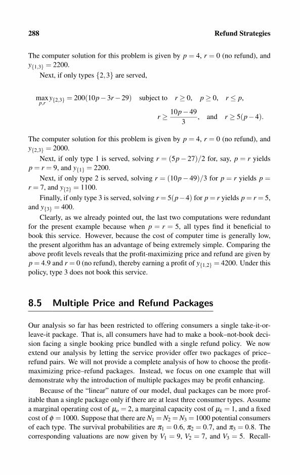
288 Refund Strategies
The computer solution for this problem is given by p = 4, r = 0 (no refund), and
y{1,3} = 2200.
Next, if only types {2,3} are served,
maxp,r
y{2,3} = 200(10p−3r−29) subject to r ≥ 0, p≥ 0, r ≤ p,
r ≥ 10p−49
3, and r ≥ 5(p−4).
The computer solution for this problem is given by p = 4, r = 0 (no refund), and
y{2,3} = 2000.
Next, if only type 1 is served, solving r = (5p− 27)/2 for, say, p = r yields
p = r = 9, and y{1} = 2200.
Next, if only type 2 is served, solving r = (10p− 49)/3 for p = r yields p =r = 7, and y{2} = 1100.
Finally, if only type 3 is served, solving r = 5(p−4) for p = r yields p = r = 5,
and y{3} = 400.
Clearly, as we already pointed out, the last two computations were redundant
for the present example because when p = r = 5, all types find it beneficial to
book this service. However, because the cost of computer time is generally low,
the present algorithm has an advantage of being extremely simple. Comparing the
above profit levels reveals that the profit-maximizing price and refund are given by
p = 4.9 and r = 0 (no refund), thereby earning a profit of y{1,2} = 4200. Under this
policy, type 3 does not book this service.
8.5 Multiple Price and Refund Packages
Our analysis so far has been restricted to offering consumers a single take-it-or-
leave-it package. That is, all consumers have had to make a book–not-book deci-
sion facing a single booking price bundled with a single refund policy. We now
extend our analysis by letting the service provider offer two packages of price–
refund pairs. We will not provide a complete analysis of how to choose the profit-
maximizing price–refund packages. Instead, we focus on one example that will
demonstrate why the introduction of multiple packages may be profit enhancing.
Because of the “linear” nature of our model, dual packages can be more prof-
itable than a single package only if there are at least three consumer types. Assume
a marginal operating cost of μo = 2, a marginal capacity cost of μk = 1, and a fixed
cost of φ = 1000. Suppose that there are N1 = N2 = N3 = 1000 potential consumers
of each type. The survival probabilities are π1 = 0.6, π2 = 0.7, and π3 = 0.8. The
corresponding valuations are now given by V1 = 9, V2 = 7, and V3 = 5. Recall-

8.5 Multiple Price and Refund Packages 289
ing (8.24), the seller is constrained to choosing price–refund packages that satisfy
r ≥ 0, p≥ 0, r ≤ p, and r ≥ p−π�V�
1−π�
for each participating type � = 1,2, . . . ,M. (8.27)
Substituting the above survival probabilities and the valuations into (8.27), the in-
difference curves of consumer types 1, 2, and 3, respectively, are given by
r = 2(5p−36), r =10p−63
3, and r =
5p−27
2(8.28)
and are drawn in Figure 8.4. In Figure 8.4, each type will book any service package
that lies on, above, or to the left of the type’s indifference curve, and will not book
any package that lies strictly below and to the right.
�
�
•
••
•
r = p3
1
p
r 2
123
A(7.2,0)
B(7.65,4.5)C(7.8,6)
D(9,9)
Figure 8.4: Dual price–refund packages with three consumer types. Thick dots, labeled A,
B, C, and D, with the (p,r) coordinates, denote potentially profitable packages.
Our main point in this demonstration is to highlight the principle behind the
sale of two different packages. This principle can be described as follows:
Threshold utility: If a consumer chooses to book the service, the utility must be
equal to or exceed the reservation level (generally normalized to equal U =0).
Rational selection: If two packages are sold to different consumers, it must be that
a buyer of the first package gains a higher utility compared with buying the
second, whereas the buyer of the second package gains a higher utility com-
pared with buying the first.
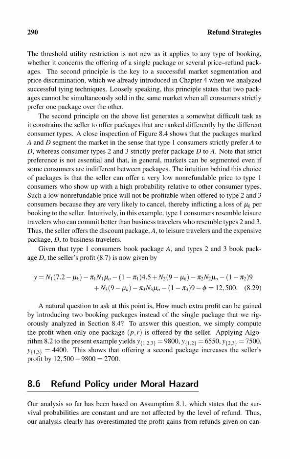
290 Refund Strategies
The threshold utility restriction is not new as it applies to any type of booking,
whether it concerns the offering of a single package or several price–refund pack-
ages. The second principle is the key to a successful market segmentation and
price discrimination, which we already introduced in Chapter 4 when we analyzed
successful tying techniques. Loosely speaking, this principle states that two pack-
ages cannot be simultaneously sold in the same market when all consumers strictly
prefer one package over the other.
The second principle on the above list generates a somewhat difficult task as
it constrains the seller to offer packages that are ranked differently by the different
consumer types. A close inspection of Figure 8.4 shows that the packages marked
A and D segment the market in the sense that type 1 consumers strictly prefer A to
D, whereas consumer types 2 and 3 strictly prefer package D to A. Note that strict
preference is not essential and that, in general, markets can be segmented even if
some consumers are indifferent between packages. The intuition behind this choice
of packages is that the seller can offer a very low nonrefundable price to type 1
consumers who show up with a high probability relative to other consumer types.
Such a low nonrefundable price will not be profitable when offered to type 2 and 3
consumers because they are very likely to cancel, thereby inflicting a loss of μk per
booking to the seller. Intuitively, in this example, type 1 consumers resemble leisure
travelers who can commit better than business travelers who resemble types 2 and 3.
Thus, the seller offers the discount package, A, to leisure travelers and the expensive
package, D, to business travelers.
Given that type 1 consumers book package A, and types 2 and 3 book pack-
age D, the seller’s profit (8.7) is now given by
y = N1(7.2−μk)−π1N1μo− (1−π1)4.5+N2(9−μk)−π2N2μo− (1−π2)9+N3(9−μk)−π3N3μo− (1−π3)9−φ = 12,500. (8.29)
A natural question to ask at this point is, How much extra profit can be gained
by introducing two booking packages instead of the single package that we rig-
orously analyzed in Section 8.4? To answer this question, we simply compute
the profit when only one package (p,r) is offered by the seller. Applying Algo-
rithm 8.2 to the present example yields y{1,2,3}= 9800, y{1,2}= 6550, y{2,3}= 7500,
y{1,3} = 4400. This shows that offering a second package increases the seller’s
profit by 12,500−9800 = 2700.
8.6 Refund Policy under Moral Hazard
Our analysis so far has been based on Assumption 8.1, which states that the sur-
vival probabilities are constant and are not affected by the level of refund. Thus,
our analysis clearly has overestimated the profit gains from refunds given on can-
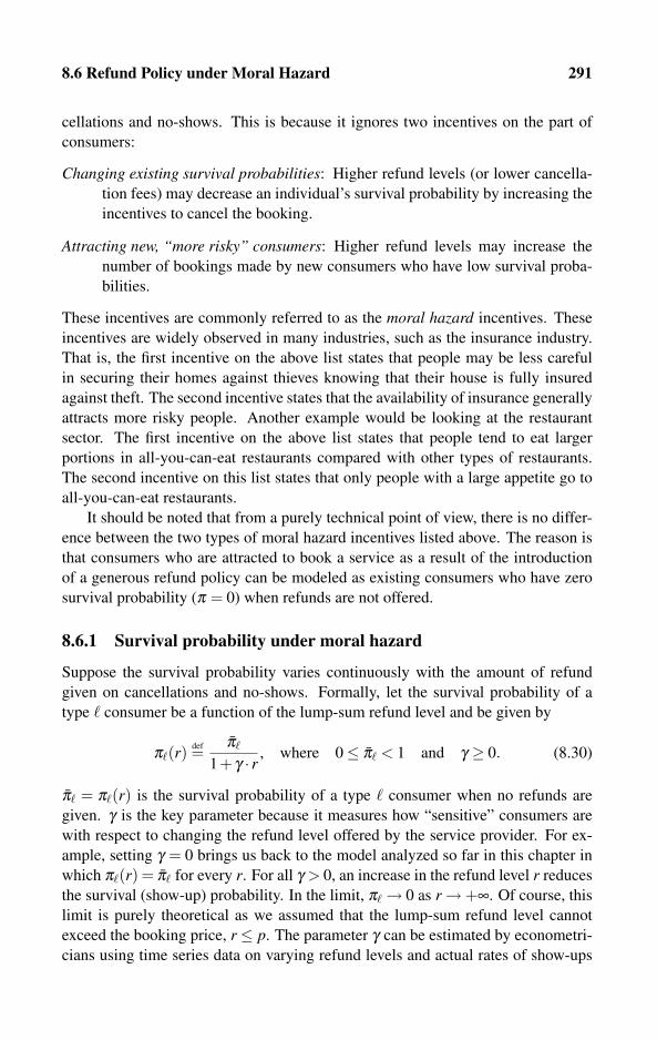
8.6 Refund Policy under Moral Hazard 291
cellations and no-shows. This is because it ignores two incentives on the part of
consumers:
Changing existing survival probabilities: Higher refund levels (or lower cancella-
tion fees) may decrease an individual’s survival probability by increasing the
incentives to cancel the booking.
Attracting new, “more risky” consumers: Higher refund levels may increase the
number of bookings made by new consumers who have low survival proba-
bilities.
These incentives are commonly referred to as the moral hazard incentives. These
incentives are widely observed in many industries, such as the insurance industry.
That is, the first incentive on the above list states that people may be less careful
in securing their homes against thieves knowing that their house is fully insured
against theft. The second incentive states that the availability of insurance generally
attracts more risky people. Another example would be looking at the restaurant
sector. The first incentive on the above list states that people tend to eat larger
portions in all-you-can-eat restaurants compared with other types of restaurants.
The second incentive on this list states that only people with a large appetite go to
all-you-can-eat restaurants.
It should be noted that from a purely technical point of view, there is no differ-
ence between the two types of moral hazard incentives listed above. The reason is
that consumers who are attracted to book a service as a result of the introduction
of a generous refund policy can be modeled as existing consumers who have zero
survival probability (π = 0) when refunds are not offered.
8.6.1 Survival probability under moral hazard
Suppose the survival probability varies continuously with the amount of refund
given on cancellations and no-shows. Formally, let the survival probability of a
type � consumer be a function of the lump-sum refund level and be given by
π�(r)def=
π�
1+ γ · r , where 0≤ π� < 1 and γ ≥ 0. (8.30)
π� = π�(r) is the survival probability of a type � consumer when no refunds are
given. γ is the key parameter because it measures how “sensitive” consumers are
with respect to changing the refund level offered by the service provider. For ex-
ample, setting γ = 0 brings us back to the model analyzed so far in this chapter in
which π�(r) = π� for every r. For all γ > 0, an increase in the refund level r reduces
the survival (show-up) probability. In the limit, π�→ 0 as r→+∞. Of course, this
limit is purely theoretical as we assumed that the lump-sum refund level cannot
exceed the booking price, r ≤ p. The parameter γ can be estimated by econometri-
cians using time series data on varying refund levels and actual rates of show-ups
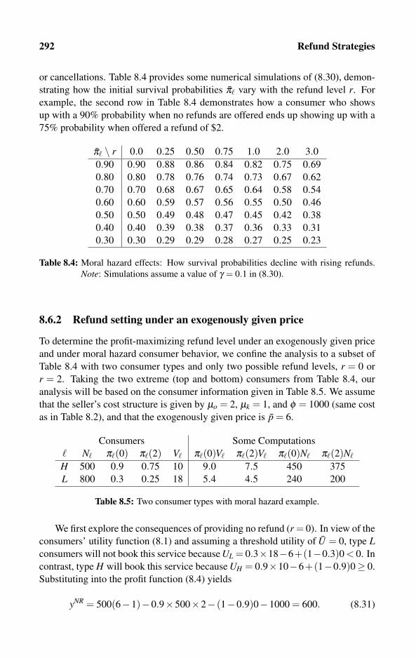
292 Refund Strategies
or cancellations. Table 8.4 provides some numerical simulations of (8.30), demon-
strating how the initial survival probabilities π� vary with the refund level r. For
example, the second row in Table 8.4 demonstrates how a consumer who shows
up with a 90% probability when no refunds are offered ends up showing up with a
75% probability when offered a refund of $2.
π� \ r 0.0 0.25 0.50 0.75 1.0 2.0 3.0
0.90 0.90 0.88 0.86 0.84 0.82 0.75 0.69
0.80 0.80 0.78 0.76 0.74 0.73 0.67 0.62
0.70 0.70 0.68 0.67 0.65 0.64 0.58 0.54
0.60 0.60 0.59 0.57 0.56 0.55 0.50 0.46
0.50 0.50 0.49 0.48 0.47 0.45 0.42 0.38
0.40 0.40 0.39 0.38 0.37 0.36 0.33 0.31
0.30 0.30 0.29 0.29 0.28 0.27 0.25 0.23
Table 8.4: Moral hazard effects: How survival probabilities decline with rising refunds.
Note: Simulations assume a value of γ = 0.1 in (8.30).
8.6.2 Refund setting under an exogenously given price
To determine the profit-maximizing refund level under an exogenously given price
and under moral hazard consumer behavior, we confine the analysis to a subset of
Table 8.4 with two consumer types and only two possible refund levels, r = 0 or
r = 2. Taking the two extreme (top and bottom) consumers from Table 8.4, our
analysis will be based on the consumer information given in Table 8.5. We assume
that the seller’s cost structure is given by μo = 2, μk = 1, and φ = 1000 (same cost
as in Table 8.2), and that the exogenously given price is p = 6.
Consumers Some Computations
� N� π�(0) π�(2) V� π�(0)V� π�(2)V� π�(0)N� π�(2)N�
H 500 0.9 0.75 10 9.0 7.5 450 375
L 800 0.3 0.25 18 5.4 4.5 240 200
Table 8.5: Two consumer types with moral hazard example.
We first explore the consequences of providing no refund (r = 0). In view of the
consumers’ utility function (8.1) and assuming a threshold utility of U = 0, type Lconsumers will not book this service because UL = 0.3×18−6+(1−0.3)0 < 0. In
contrast, type H will book this service because UH = 0.9×10⁻⁶+(1−0.9)0≥ 0.
Substituting into the profit function (8.4) yields
yNR = 500(6−1)−0.9×500×2− (1−0.9)0−1000 = 600. (8.31)
8.7 Integrating Refunds within Advance Booking 293
Next, suppose the seller promises a lump-sum refund of r = 2 on no-shows.
Type L consumers will book this service because UL = 0.25× 18− 6 + (1−0.25)2 ≥ 0. Type H consumers will also book this service because UH = 0.75×10⁻⁶+(1−0.75)2≥ 0. Substituting into the profit function (8.4) yields
yPR = (500+800)(6−1)− (0.75×500+0.25×800)2
− [(1−0.75)500+(1−0.25)800]2−1000 = 2900 > yNR. (8.32)
Hence, in this example, providing a refund of r = 2 yields a higher profit than
providing no refund, despite the fact that refunds reduce consumers’ survival prob-
abilities.
From a practical point of view, the above example suggests one method for how
to compute the profit-maximizing refund level given that consumers’ tendency to
cancel or not show intensifies with an increase in the promised refund level. These
corrections can be embedded into a computer algorithm by substituting the value of
the estimated value of γ into the survival probabilities given by (8.30). The reader
is referred to Exercise 10, which provides a good example of how an increase in
the refund level leads to an exclusion of type H consumers from the market. In
this exercise a high refund leaves the seller serving only the consumers with low
survival probabilities.
8.7 Integrating Refunds within Advance Booking
A computer reservation system should integrate all aspects of advance booking,
which include the advance booking algorithms analyzed in Chapter 7, the over-
booking analyzed in Chapter 9, and the options to give refunds or charge cancella-
tion fees that we analyze in the present chapter.
This short section attempts to suggest one possible way to integrate the advance
booking algorithms developed in Chapter 7 with the refund and cancellation fee
options analyzed in the present chapter. Note, however, that our comprehensive
analysis of advance booking in Chapter 7 lacked an algorithm for selecting profit-
maximizing prices. That is, our dynamic booking algorithms were all based on
predetermined exogenously given prices (that could vary among booking classes).
Because refund decisions are basically part of pricing decisions, there is really no
general method to integrate the advance booking algorithms with pricing and refund
decisions.
However, because many service providers who are engaged in advance booking
may also find it profitable to offer some refunds, we propose the following three-
stage methodology for how to integrate these algorithms.
(1) Pricing and refund determination: Use the techniques from this chapter as well
as Chapter 3 to determine the profit-maximizing price and refund levels.
294 Refund Strategies
(2) Compute the average survival probability: For consumers your model predicts
will book the service, compute the average survival probability by
π = ∑M�=1 (n� ·π�)∑M
�=1 n�
,
where n� = N� for participating types, and n� = 0 otherwise.
(3) Modify the advance booking algorithm: Redefine the class fares so that for
each booking class i ∈B, pi def= π pi +(1− π)(pi− r).
The third step simply “lowers” the class fare to the expected revenue from each
booking, taking into account the possibility of a no-show. The reader should not
confuse the survival probabilities π and π� with the probabilities of booking each
class i, i ∈B.
Finally, the second step may be needed because the advance booking analysis
in Chapter 7 was confined to a single price (per class), hence, we basically mod-
eled a single consumer type. In contrast, this chapter allows for multiple types
(according to survival probability and willingness to pay). In fact, the gains from
giving refunds can be realized only if there are at least two consumer types. Hence,
by averaging the survival probabilities of consumers who book the service, we
may be able to obtain an approximate value of the average survival probability π .
Obviously, the second step is not needed if the seller already knows the survival
probabilities for each booking class.
8.8 Exercises
1. Consider a consumer who can book a service for the price of p and obtain a
refund of r in the event the consumer cancels. We now modify the consumer’s
utility function given by (8.1) to be
U(p,r) def=
{πV − p+(1−π)r if he or she books the service
3 does not book this service.
Thus, the consumer now has a threshold utility level of U = 3. Similar to Ta-
ble 8.1, fill in the missing entries in Table 8.6.
2. Suppose V = 10 and π = 0.5. Solve the following problems.
(a) Similar to Figure 8.1, draw the consumer’s indifference curve concerning
the book–no-book decision for the utility function given in Exercise 1 (with
the threshold utility U = 3).
(b) Infer the maximum price the consumer will be willing to pay for booking
this service, assuming that no refund is given (r = 0). Show your calcula-
tions.

8.8 Exercises 295
π V πV p r (1−π)r U Decision
0.8 20 13 0
0.8 20 14 2
0.9 20 16 9
0.2 20 4 3
Table 8.6: Refunds and booking decisions for Exercise 1.
(c) Infer the maximum price a consumer will be willing to pay for booking the
service assuming a full refund (r = p). Show your calculations.
3. Consider the two-consumer example given by Table 8.2. Similar to our analysis
in Section 8.3.1, compute the profit-maximizing refund level assuming that the
exogenously given price has been reduced to p = 4 (instead of p = 6). Show
you calculations.
4. Consider the two-consumer example given by Table 8.2 in Section 8.3.1, but
suppose now that the exogenously given price is p = 7 and that the cost param-
eters are now given by μo = 2, μk = 3, and φ = 1200.
(a) Compute the service provider’s profit level given that no refunds are offered
to consumers.
(b) Compute the profit level given that this seller provides full refunds on no-
shows.
(c) Compute the profit-maximizing refund level.
5. Consider the three consumer–type example described by Table 8.3. How-
ever, assume that the exogenously given price is now p = 7. Compute the
profit-maximizing lump-sum refund level using the algorithm developed in Sec-
tion 8.3.1.
6. Consider our analysis of proportional refunds given in Section 8.3.2. Compute
the profit-maximizing refund rate 0≤ r ≤ 1 under the conditions listed in Exer-
cise 4.
7. Consider the seller’s problem of simultaneously setting the price and refund
levels when there are only two consumer types, as studied in Section 8.4.1.
Assume a marginal operating cost of μo = 2, a marginal capacity cost of μk = 1,
and no fixed costs, so φ = 0. Suppose there are NH = NL = 1000 potential
consumers of each type. The survival probabilities are πH = 0.9 and πL = 0.5.
Compute the profit-maximizing price and refund level under the following two
different cases: (a) VH = 5 and VL = 7 and (b) VH = 7 and VL = 6.

296 Refund Strategies
8. Consider the seller’s problem of simultaneously setting the price and refund lev-
els with multiple consumer types, studied in Section 8.4.2. Assume a marginal
operating cost of μo = 2, a marginal capacity cost of μk = 1, and no fixed costs,
so φ = 0. Suppose there are N1 = N2 = 100 and N3 = 200 potential consumers
of each type. The survival probabilities are π1 = 0.9, π2 = 0.8, and π3 = 0.7.
The valuations are now given by V1 = 9, V2 = 8, and V3 = 7. Using the proce-
dure described by Algorithm 8.2, and any basic linear programming software,
compute the profit-maximizing price and refund level.
9. Consider the moral hazard model of Section 8.6. Suppose there is only one
type of consumer whose survival probabilities are given in the bottom row of
Table 8.4. Assume that consumers’ basic valuation for the service is V = 18
and that the booking price is fixed at the level of p = 6. Using the bottom
row of Table 8.4 and the utility function (8.1), compute the minimum refund
level under which the consumers of this type will find it beneficial to book this
service. Show your calculations.
10. Consider our moral hazard example with two consumer types displayed in Ta-
ble 8.5. Suppose now that the service valuation of type H consumers is now
VH = 7 (instead of VH = 10). Suppose the service provider is restricted to set-
ting either no refund (r = 0) or a lump-sum refund level of r = 2. Compute
which refund level maximizes the expected profit of this service provider as-
suming the booking price is p = 6 and the cost structure is given by μo = 2,
μk = 1, and φ = 1000.

Chapter 9
Overbooking
9.1 Basic Definitions 2999.1.1 Show-up probabilities
9.1.2 Overbooking and probability
9.2 Profit-maximizing Overbooking 3059.2.1 Expected cost
9.2.2 Expected revenue and expected profit
9.2.3 Simple examples
9.2.4 Computer algorithm
9.3 Overbooking of Groups 3139.3.1 Simple examples
9.3.2 General formulation
9.3.3 Computer algorithm
9.4 Exercises 322
We define overbooking as a strategy whereby service providers accept and confirm
more reservations than the capacity they allocate for providing the service. Thus,
the overbooking strategy may result in service denial to some consumers if the
number of actual show-ups at the time of service exceeds the allocated capacity.
Overbooking should be considered an integral part of the advance booking strat-
egy of service providers. In this chapter, we demonstrate how service providers
can increase their profits by using overbooking. Thus, in this chapter, we relax
Assumption 7.3, which so far has ruled out the use of the overbooking strategy.
From a practical point of view, the dynamic booking models analyzed in Chap-
ter 7 can be modified to accommodate overbooking by letting the booking capac-
ity K exceed the available capacity level during all booking periods. However,
maintaining the same “artificially high” capacity level throughout the entire book-
ing process need not be optimal because it may be more profitable to reduce the
amount of overbooking as the reservation period gets closer to the service delivery
time. In other words, it may be profitable to allow for a large overbooking level
298 Overbooking
at the beginning of the booking process, but lower levels toward the end, when
the service provider can more accurately estimate the final number of reservations
made and the expected number of show-ups. Despite this discussion, in this chap-
ter, we do not attempt to integrate overbooking with the dynamic booking models
of Chapter 7. Instead, we develop an independent model for computing the profit-
maximizing booking levels.
We first must ask why service providers may find it profitable to overbook
consumers. The answer to this question is that it is commonly observed that a
large number of reservations end up being cancelled by consumers and a somewhat
smaller number of consumers simply do not show up at the time of service. Cancel-
lations and no-shows have already been discussed in Chapter 8 where we analyzed
refund policies. In fact, the reader is urged to consult Definition 8.1, which makes a
clear distinction between cancellations and no-shows. To illustrate this distinction,
let us look at the airline industry, for example, in which the data of domestic fights
in the United States show that 30–60% of reservations eventually get cancelled,
whereas the no-show rate is around 8%. These data clearly indicate that booking
up to capacity only will result in a significant amount of unused capacity during the
service delivery time (the commonly observed problem of empty seats in the airline
industry). The second question we may want to ask is whether consumers can ben-
efit from overbooking. A quick answer to this question would be that overbooking
enables more consumers to make reservations.
Overbooking is widely observed in the airline industry. In fact, most readers
would recognize the following statement, which is printed on most ordinary airline
tickets.
Airline flights may be overbooked, and there is a slight chance that
a seat will not be available on a flight for which a person has a con-
firmed reservation. If the flight is overbooked, no one will be denied
a seat until airline personnel first ask for volunteers willing to give up
their reservation in exchange for a payment of the airline’s choosing.
If there are not enough volunteers, the airline will deny boarding to
other persons in accordance with its particular boarding priority. With
few exceptions, persons denied boarding involuntarily are entitled to
compensation. The complete rules for the payment of compensation
and each airline’s boarding priorities are available at all airport ticket
counters and boarding locations.
In the airline industry, passengers with confirmed reservations who are denied
boarding must be offered the choice of a full refund for the ticket or an alternative
flight to continue their journey. Furthermore, the carrier should supply meals and
refreshments, and accommodation if an overnight stay is required. In addition,
since 2005, European Union regulations require airlines to pay denied passengers
an amount of e 250 for flights up to 1500 kilometers, e 400 for flights between

9.1 Basic Definitions 299
1500 and 3500 kilometers, and e 600 for longer flights. In the United States, the
mandated payment is limited to 200% of the value of the remaining flight coupons,
not exceeding $400.
Overbooking has been analyzed in operational research, transportation, and
economics literature; see comprehensive surveys by Belobaba (1987), Rothstein
(1985), and McGill and van Ryzin (1999). Other papers include Shlifer and Vardi
(1975), Bodily and Pfeifer (1992), and Ringbom and Shy (2002).
9.1 Basic Definitions
A single service provider has the capacity to accommodate a maximum of K cus-
tomers. This provider decides how many booking requests to accept, which we
denote by the decision variable b. Our assumption is that the number of book-
ing requests is sufficiently large in the sense that it far exceeds the capacity level
K. For example, K could be measuring the seating capacity available on a certain
flight using a certain aircraft type. In this example, b is the number of passenger
reservations confirmed by the airline before the time of service.
In many regulated and partially regulated industries, the regulator may limit
the number of allowable overbookings. Even when the regulator does not im-
pose any limit, the service provider may want to set a level beyond which no more
consumers can be booked to avoid severe reputation effects. We denote this level
by B to indicate that the service provider programs the reservation system never to
accept booking requests beyond b = B. Formally, b > B is ruled out by the booking
system. Booking limits are often described in percentage terms relative to capac-
ity. For example, an overbooking limit of 30% would mean that an airline cannot
book more than B = 130 passengers on a flight served by an aircraft with a seating
capacity of K = 100.
9.1.1 Show-up probabilities
Let π (0 < π ≤ 1) denote the probability that a consumer with a confirmed reser-
vation actually shows up at the service delivery time. In the professional language,
this probability is often referred to as a consumer’s survival probability. We as-
sume that all consumers have the same show-up probability, and that a consumer’s
show-up probability is independent of all other consumers. That is, we rule out
events such as last-minute group cancellations and no-shows, which are analyzed
later in Section 9.3. In this chapter, we learn how to compute the expected number
of show-ups for each booking level, b. Formally, let the random variable s denote
the number of consumers who show up at the service delivery time. Clearly, s≤ b,
meaning that the number of show-ups cannot exceed the number of bookings. That
is, our model does not allow for standby customers, and only customers with con-
firmed reservations are provided with this service. In fact, because s depends on

300 Overbooking
the number of bookings made, s is a function of b and will often be written as
s(b). Also, note that s is a random variable, which also depends on the individual’s
show-up probability π , hence it can also be written as s(b ;π).We start out with simple examples showing how to compute the probability
of realizing different numbers of show-ups (different realizations of the random
variable s). Suppose that the service provider confirms one reservation only. That
is, let b = 1. Then, the probability that this booked consumer shows up is Pr{s(1) =1}= π , whereas the probability that no consumer shows up is Pr{s(1) = 0}= 1−π .
Next, suppose that there are b = 2 confirmed reservations. The probability that
exactly one consumer shows up is given by
Pr{s(2) = 1}= π(1−π)︸ ︷︷ ︸1st arrives, 2nd not
+ (1−π)π︸ ︷︷ ︸1st not, 2nd arrives
= 2π(1−π).
The probability that both consumers show up is then Pr{s(2) = 2}= π2.
Suppose now that this service provider books three consumers so that b = 3.
The probability that no one shows up is Pr{s(3) = 0} = (1−π)3. The probability
that exactly one consumer arrives is given by
Pr{s(3) = 1} = π(1−π)(1−π)︸ ︷︷ ︸1st yes, 2nd no, 3rd no
+(1−π)π(1−π)︸ ︷︷ ︸1st no, 2nd yes, 3rd no
+(1−π)(1−π)π︸ ︷︷ ︸1st no, 2nd no, 3rd yes
= 3π(1−π)2. (9.1)
Using the same logic, we can compute the probability that exactly two consumers
show up to be
Pr{s(3) = 2} = π ·π(1−π)︸ ︷︷ ︸1st yes, 2nd yes, 3rd no
+ (1−π)π ·π︸ ︷︷ ︸1st no, 2nd yes, 3rd yes
+ π(1−π)π︸ ︷︷ ︸1st yes, 2nd no, 3rd yes
= 3π2(1−π). (9.2)
Next, the probability that all three consumers with confirmed reservations show up
is Pr{s(3) = 3}= π3. Now, if we take for example a survival probability of π = 0.8,
we obtain Pr{s(3) = 0} = 0.23 = 0.008, Pr{s(3) = 1} = 3× 0.8× 0.22 = 0.096,
Pr{s(3) = 2} = 3×0.82×0.2 = 0.348, and Pr{s(3) = 3} = 0.83 = 0.512. Notice
that the sum of all these probabilities is equal to one because they reflect all the
possible show-up events given that three consumers are booked for this service.
Finally, it would be interesting to check whether, or under what conditions, the
probability that exactly two consumers show up exceeds the probability that exactly
one consumer shows up. Formally, the following computation reveals that
Pr{s(3) = 2} ≥ Pr{s(3) = 1}⇐⇒ 3π2(1−π)≥ 3π(1−π)2⇐⇒ π ≥ 1
2.
That is, the probability that exactly two consumers show up is higher than the prob-
ability that only one consumer shows up if the survival probability exceeds 50%.

9.1 Basic Definitions 301
Similarly, the probability that three consumers show up exceeds the probability that
only two consumers show up if
Pr{s(3) = 3} ≥ Pr{s(3) = 2}⇐⇒ π3 ≥ 3π2(1−π)⇐⇒ π ≥ 2
3.
The above examples demonstrate that it is useful to have a general formula for
computing the probability that exactly s consumers show up given that b consumers
have confirmed reservations for the service. This formula becomes essential for
larger values of b, and is given by the following binomial distribution function:
Pr{s(b) = s}=b !
s ! (b− s)!π s(1−π)b−s for 0≤ s≤ b. (9.3)
The intuition behind the formula given in (9.3) is as follows: The term π s is the
probability that precisely s specific people (who we can identify by their names,
say) show up. The term (1−π)b−s is the probability that precisely b− s specific
people (who again we can identify by their names) do not show up. The first term,
sometimes written as(b
s
)and referred to as “b choose s,” computes the number of
times that any s people can be “pooled” from a group of b consumers. We should
note again that the distribution function given by (9.3) relies on the assumption
that consumers’ actions regarding showing up at the time of service are indepen-dent. Thus, (9.3) rules out last-minute group cancellations and no-shows, which
are analyzed later in Section 9.3.
To practice the use of the formula given by (9.3), let us recompute (9.1), which
is the probability that exactly one consumer out of three confirmed reservations will
show up. In this case,
Pr{s(3) = 1}=3!
1! (3−1)!π1(1−π)3−1 =
3!
1! ·2!π1(1−π)2 = 3π(1−π)2.
Consider now another example that makes use of the binomial distribution.
Suppose that an airline confirms 120 reservations on a certain flight. Then, (9.3)
implies that the probability that exactly 118 passengers show up for this flight is
Pr{s(120) = 118}=120!
118! ·2!π118(1−π)2 = 7140 ·π118(1−π)2.
To take a more specific example, if we assume that the survival probability is π =0.99, the above computation implies that Pr{s(120) = 118}= 0.2180977445.
We conclude our analysis of the binomial distribution with the computation
of the expected number of show-ups. As it turns out, the binomial distribution
defined by (9.3) generates a very simple formula for the expected number of show-
ups. Without providing a formal proof, we merely state that if the service provider
books b consumers, the expected number of show-ups is given by
Es(b) =b
∑s=0
Pr{s(b) = s} · s = π ·b, (9.4)
302 Overbooking
which is the survival probability of each individual multiplied by the number of
bookings made by the service provider. For example, if the survival probability is
π = 0.8 and the service provider books b = 120 consumers, the expected number
of show-ups is Es(b) = 0.8×120 = 96 consumers.
9.1.2 Overbooking and probability
We now make use of our assumption that the service provider has a capacity con-
straint of admitting no more than K consumers at the time of service. Overbooking
is defined as follows:
DEFINITION 9.1
We say that a service provider is engaged in overbooking consumers if the number
of confirmed reservations exceeds the service capacity level; that is, if b≥ K +1.
The reader is urged to consult the notation described in Tables 1.4 and 1.5 to recall
that b (lowercase letter) denotes a choice variable, whereas K (capital letter) denotes
an exogenously given parameter. Thus, Definition 9.1 identifies which booking
levels are regarded as overbooking. The purpose of this chapter is to provide a
method for computing the profitable amount of overbooking. A high overbooking
level may result in high penalties to be paid to customers who are denied service.
Underbooking is likely to result in some unfilled capacity due to no-shows. In this
chapter, we weigh this trade-off to find the exact profit-maximizing booking level,
b.
A major possible consequence of overbooking is described by the following
definition:
DEFINITION 9.2
Suppose that service provider books b consumers. If the number of show-ups
exceeds the available capacity level, formally if s(b) ≥ K + 1, then we say that
ds(b) def= s(b)−K consumers are denied service.
An alternative terminology for denied service that is commonly used in the airline
industry is to say that ds passengers are “bumped” from a flight. Note that the
number of consumers who are denied service is affected by the number of bookings
made, because the number of show-ups s(b) is also a function of the number of
bookings, b, made by the service provider.
We now proceed to computing the probabilities of overbooking events. Sup-
pose that the service provider overbooks, so b≥K +1. The probability that exactly
one consumer is denied service is given by
Pr{ds(b) = 1}= Pr{s(b) = K +1}=
b!
(K +1)! (b−K−1)!πK+1(1−π)b−K−1.

9.1 Basic Definitions 303
More generally, the probability that exactly ds consumers are denied service given
that consumers hold b confirmed reservations is
Pr{ds(b) = ds}= Pr{s(b) = K +ds}=
b!
(K +ds)! (b−K−ds)!πK+ds(1−π)b−K−ds, (9.5)
for all denied service levels satisfying 1≤ ds≤ b−K.
Let us now practice the use of (9.5) with the following example: Consider
an airline that books b = 104 passengers on an aircraft with a seating capacity
of K = 100. We now compute the probabilities that ds = 1,2,3,4 consumers are
denied service:
Pr{ds(104) = 1} = Pr{s(104) = 101}=104!
101! ·3!π101(1−π)3
= 182104 π101(1−π)3.
Pr{ds(104) = 2} = Pr{s(104) = 102}=104!
102! ·2!π102(1−π)2
= 5356 π102(1−π)2. (9.6)
Pr{ds(104) = 3} = Pr{s(104) = 103}=104!
103! ·1!π103(1−π)1
= 104 π103(1−π)1.
Pr{ds(104) = 4} = Pr{s(104) = 104}=104!
104! ·0!π104(1−π)0 = π104.
A natural question to ask at this point is, What is the probability that at leastone consumer is denied service? Using the above example, this probability is given
by the sum
Pr{ds(104)≥ 1}= Pr{ds(104) = 1}+Pr{ds(104) = 2}+Pr{ds(104) = 3}+Pr{ds(104) = 4}.
Clearly, the probability that no one is denied service is simply one minus the above
probability, that is, 1−Pr{ds(104) ≥ 1}. More generally, we can write the proba-
bility that at least one consumer is denied service when the service provider owns
K capacity units and books b consumers, where b≥ K +1, as
Pr{ds(b)≥ 1}=b−K
∑ds=1
Pr{ds(b) = ds}. (9.7)
Hence, the probability that no one is denied service is
Pr{ds(b) = 0}= 1−Pr{ds(b)≥ 1}= 1−b−K
∑ds=1
Pr{ds(b) = ds}. (9.8)

304 Overbooking
Clearly, we can also express the probabilities that overbooking occurs and does
not occur directly as a function of the number of show-ups, s(b). That is, we can
rewrite (9.7) as
Pr{ds(b)≥ 1}= Pr{s(b)≥ K +1}=b
∑s=K+1
Pr{s(b) = s}
=b
∑s=K+1
b!
s ! (b− s)!π s(1−π)b−s. (9.9)
Similarly, we can rewrite (9.8) as
Pr{ds(b) = 0}= Pr{s(b)≤ K}=K
∑s=0
Pr{s(b) = s}
=K
∑s=0
b!
s ! (b− s)!π s(1−π)b−s. (9.10)
That is, the probability computed in (9.7) is identical to (9.9), and the probability
computed in (9.8) is identical to (9.10). The probability computed in (9.8) is one
minus the probability that at least one consumer is denied service, whereas (9.10) is
the sum of probabilities of all possible show-up levels s not exceeding the capacity
level K. Clearly, both computation methods yield identical results.
We conclude our analysis of service denial with the computation of the ex-
pected number of consumers who are denied service. Suppose again that con-
sumers’ survival probability is π , service capacity level is K, and b consumers are
booked. Clearly, if b≤K, the number of consumers expected to be denied service is
Eds(b) = 0 because there is no overbooking of consumers. However, if b≥ K +1,
the number of consumers expected to be denied service is given by
Eds(b) =K
∑s=0
Pr{s(b) = s} ·0︸ ︷︷ ︸
s(b)≤K =⇒ ds(b)=0
+b
∑s=K+1
Pr{s(b) = s} (s−K)
︸ ︷︷ ︸s(b)≥K+1 =⇒ ds(b)=s−K
. (9.11)
Substituting (9.3) into (9.11) yields the general formula for the expected number of
consumers who are denied service given that there are b confirmed reservations for
K units of capacity. Therefore,
Eds(b) =
⎧⎪⎨⎪⎩
0 if b≤ Kb
∑s=K+1
b!
s! (b− s)!πs(1−π)b−s (s−K) if b≥ K +1.
(9.12)
That is, the number of consumers expected to be denied service is the sum of the
probabilities of all show-up realizations beyond capacity multiplied by the number
of consumers who are denied service.
9.2 Profit-maximizing Overbooking 305
It is important to note that the expected number given by (9.12) cannot be de-
rived directly from the formula for the expected number of show-ups given by (9.4).
This follows from the observation that in most cases Eds(b) �= E[s(b)−K], because
we must set ds(b) = 0 (rather than ds(b) < 0) for show-up realizations satisfying
s(b)−K < 0. Another way of explaining this difference is to observe that the ex-
pected number of show-ups (9.4) is independent of the difference b−K, whereas
the expected number of consumers who are denied service clearly depends on this
difference.
9.2 Profit-maximizing Overbooking
The purpose of designing an overbooking plan is to maximize expected profit, tak-
ing into consideration that a certain fraction of customers with confirmed reserva-
tions will not show up at the time of service. We use the statistical term expectedbecause service providers are subjected to random realizations of the number of
consumers who show up at the time of service. Moreover, with some probability
(which was computed in the previous section), overbooking can be highly costly to
service providers when the number of consumers who show up at the time of ser-
vice exceeds the given capacity level K. Formally, our investigation of the profit-
maximizing booking level should take into consideration that a sufficiently high
booking level b, where b≥ K +1, and a sufficiently low survival probability π will
result in having ds = s(b)−K consumers being denied service.
9.2.1 Expected cost
Service providers bear four types of costs: fixed and sunk costs denoted by φ , which
are independent of the number of people who book the service and the number of
show-ups; per-customer capacity cost, denoted by μk; and per-customer operating
cost, denoted by μo. The reader is referred to Definition 8.4 for a more precise
distinction between marginal capacity cost and marginal operating cost. The fourth
type of cost borne by service providers is the marginal cost of denying service to a
booked consumer. We denote this penalty rate by ψ . The penalty rate ψ consists of
a direct payment to a consumer who is denied service and also includes some un-
observed reputation and goodwill-related costs that may affect future reservations
made by a consumer who is denied service.
In this chapter, we assume that the service provider has already allocated Kunits of capacity that is capable of serving K customers. Under this assumption, the
service provider bears a cost of φ + μkK independent of the number of bookings.
Thus, only the operating cost μo and the penalty rate ψ are relevant for determin-
ing how total cost increases with an increase in the booking level b. Formally, if
s(b) consumers show up, the realized total cost of a service provider who books b

306 Overbooking
consumers is given by
c(s(b)) =
{φ + μkK + μoK +ψ[s(b)−K] if s(b)≥ K +1
φ + μkK + μos(b) if s(b)≤ K.(9.13)
That is, in the event of a large number of show-ups so that s(b)≥K +1, the service
provider must deny service to ds = s(b)−K confirmed customers and pay a penalty
that sums up to ψ · ds = ψ[s(b)−K]. Because capacity is fully used, the sum of
capacity and operating cost is simply (μk +μo)K. The second line in (9.13) reflects
the cost when (over- or under-) booking does not result in denied service as the
number of show-ups does not exceed capacity. In this case, the firm bears the
given capacity cost μkK and the variable operating cost μos(b) that depends on the
realization of the random show-up variable s(b).We wish to express the total cost function (9.13) in expected terms using
the probabilities computed in (9.3), (9.5), (9.9), and (9.10). Thus, if the service
provider overbooks, that is, if b≥ K +1,
c(b) = φ + μkK︸ ︷︷ ︸fixed costs
+K
∑s=0
Pr{s(b) = s} μos
︸ ︷︷ ︸expected operating cost for s(b)≤ K
+b
∑s=K+1
Pr{s(b) = s} [μoK +ψ(s−K)].
︸ ︷︷ ︸expected operating & penalty costs for s(b)≥ K +1
(9.14)
The second term is the expected operating cost when there is no service denial
when the number of show-ups does not exceed capacity. The last term is the sum of
operating cost and penalty incurred when the number of show-ups exceeds capacity
so that s−K customers must be denied service. In this case, the operating cost
equals μoK because the firm cannot accommodate more than K customers.
The expected cost (9.14) is formulated for the case of overbooking, b≥ K +1.
However, if the service provider does not overbook consumers, that is, if b≤K, the
expected total cost given by (9.14) becomes
c(b) = φ + μkK︸ ︷︷ ︸fixed costs
+b
∑s=0
Pr{s(b) = s} μos.
︸ ︷︷ ︸expected operating cost for s(b)≤ b≤ K
(9.15)
Observe that the upper limit of the summation in the second term of (9.14) is K(full capacity), whereas the upper limit of the second term in (9.15) is only b < K(booking below capacity).

9.2 Profit-maximizing Overbooking 307
Substituting (9.3) into (9.14), the explicit formulation of the expected cost of a
service provider that overbooks customers (b≥ K +1) is given by
c(b) = φ + μkK +K
∑s=0
b!
s! (b− s)!πs(1−π)b−s μo s
+b
∑s=K+1
b!
s! (b− s)!πs(1−π)b−s [μoK +ψ(s−K)]. (9.16)
The formulation of the expected cost functions under overbooking, given by
(9.14) and (9.16), reveal that solving overbooking problems requires the separation
of all possible events into two groups. First, when the number of show-ups falls
short of capacity, s(b) ≤ K. Second, when the number of show-ups exceeds ca-
pacity, s(b) ≥ K + 1. In the second case, ds(b) = s(b)−K consumers are denied
service, in which case the operating cost becomes a constant μoK that is indepen-
dent of the number of show-ups. This happens because only K consumers can be
served.
9.2.2 Expected revenue and expected profit
We now compute a service provider’s expected revenue as a function of the number
of bookings b. Assume that the service provider offers the service for an exoge-
nously given price denoted by P. Because P is written in a capital letter, it is treated
as an exogenous parameter of the model developed in this chapter (compare P in
Table 1.4 with p in Table 1.5). Also, assume that P > μk + μo, which means that
the price exceeds the sum of marginal capacity cost and marginal operating cost.
Clearly, the price should be even higher than this sum to cover the fixed cost φ .
Assuming otherwise implies that the service provider makes a loss on each unit of
sales, and hence must shut down.
Similar to our discussion about cost in Section 9.2.1, and because the revenue
also depends on the realization of the number of show-ups s(b), we must distinguish
between two sets of events, depending on whether the number of show-ups is below
capacity or exceeds capacity. Hence, the expected revenue to be collected by a
service provider who books b consumers is given by
x(b) =⎧⎪⎪⎪⎪⎪⎪⎪⎪⎪⎨⎪⎪⎪⎪⎪⎪⎪⎪⎪⎩
b
∑s=0
Pr{s(b) = s} Ps
︸ ︷︷ ︸expected revenue for s(b)≤ b≤ K
if b≤ K
K
∑s=0
Pr{s(b) = s} Ps
︸ ︷︷ ︸expected revenue for s(b)≤ K
+b
∑s=K+1
Pr{s(b) = s} PK
︸ ︷︷ ︸expected revenue for s(b)≥ K +1
if b≥ K +1.
(9.17)
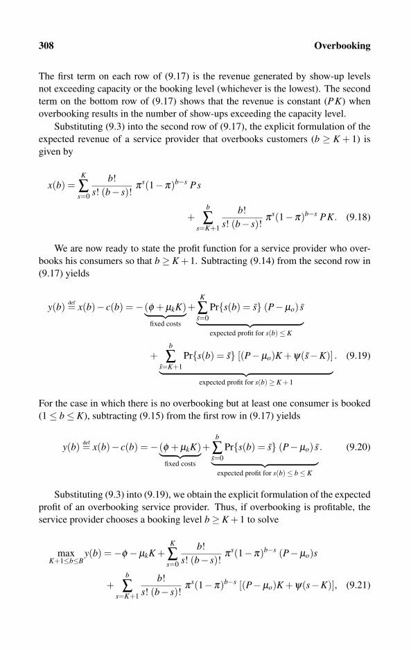
308 Overbooking
The first term on each row of (9.17) is the revenue generated by show-up levels
not exceeding capacity or the booking level (whichever is the lowest). The second
term on the bottom row of (9.17) shows that the revenue is constant (PK) when
overbooking results in the number of show-ups exceeding the capacity level.
Substituting (9.3) into the second row of (9.17), the explicit formulation of the
expected revenue of a service provider that overbooks customers (b ≥ K + 1) is
given by
x(b) =K
∑s=0
b!
s! (b− s)!πs(1−π)b−s Ps
+b
∑s=K+1
b!
s! (b− s)!πs(1−π)b−s PK. (9.18)
We are now ready to state the profit function for a service provider who over-
books his consumers so that b≥ K +1. Subtracting (9.14) from the second row in
(9.17) yields
y(b) def= x(b)− c(b) =−(φ + μkK)︸ ︷︷ ︸fixed costs
+K
∑s=0
Pr{s(b) = s} (P−μo) s
︸ ︷︷ ︸expected profit for s(b)≤ K
+b
∑s=K+1
Pr{s(b) = s} [(P−μo)K +ψ(s−K)]
︸ ︷︷ ︸expected profit for s(b)≥ K +1
. (9.19)
For the case in which there is no overbooking but at least one consumer is booked
(1≤ b≤ K), subtracting (9.15) from the first row in (9.17) yields
y(b) def= x(b)− c(b) =−(φ + μkK)︸ ︷︷ ︸fixed costs
+b
∑s=0
Pr{s(b) = s} (P−μo) s
︸ ︷︷ ︸expected profit for s(b)≤ b≤ K
. (9.20)
Substituting (9.3) into (9.19), we obtain the explicit formulation of the expected
profit of an overbooking service provider. Thus, if overbooking is profitable, the
service provider chooses a booking level b≥ K +1 to solve
maxK+1≤b≤B
y(b) =−φ −μkK +K
∑s=0
b!
s! (b− s)!πs(1−π)b−s (P−μo)s
+b
∑s=K+1
b!
s! (b− s)!πs(1−π)b−s [(P−μo)K +ψ(s−K)], (9.21)

9.2 Profit-maximizing Overbooking 309
where B is the maximum allowable booking level. In the case in which underbook-
ing is profitable, substituting (9.3) into and (9.20), the service provider should also
solve
max0≤b≤K
y(b) =⎧⎪⎨⎪⎩
0 if b = 0
−φ −μkK +b
∑s=0
b!
s! (b− s)!πs(1−π)b−s (P−μo)s if b≥ 1.
(9.22)
The profit-maximization booking level b∗ is chosen as the booking level that
yields the highest profit level obtained from solving (9.21) and (9.22). However,
because of the linear property of the present model, the solution to (9.22) yields
either b∗ = 0 with y(b∗) = 0 (no booking at all) or b∗ = K (booking exactly to full
capacity). This means that to find b∗, we need to compare only the profit levels
given by y(0), y(K), and the profit level that solves (9.21).
9.2.3 Simple examples
The following examples demonstrate the logic behind a profitable determination
of the overbooking level. These examples are simple in the sense that they do not
necessarily require the use of computers, as most of these examples can be solved
even without making use of the binomial distribution formula (9.3). In all examples,
we continue to assume that the fixed and capacity costs given by φ +μkK are borne
only if the service provider books at least one consumer. Otherwise, if no bookings
are made by the service provider (b = 0), the firm earns zero profits, so y(0).
How to overbook a single unit of capacity
Suppose that the service provider can accommodate at most one consumer, so
K = 1. Assume that the regulator restricts overbooking to not exceed 300% of
capacity, which translates in the present example to assuming that B = 3. We first
compute the expected profit levels y(b) for booking levels b = 0,1,2,3, assum-
ing a general survival probability π . Then, we proceed with some more specific
numerical examples by substituting specific numbers for the parameter π .
If the service provider does not book any consumer, no profit or loss are made
as we assumed that y(0) = 0. Next, if the firm books at least one consumer, the sum
of the fixed and capacity costs is φ + μk for all booking levels b≥ 1. When exactly
one booking is made, b = 1, the resulting expected profit is given by
y(1) = − (φ + μk)︸ ︷︷ ︸fixed & capacity costs for K = 1
+ π(P−μo)︸ ︷︷ ︸case s(1)=1
, (9.23)
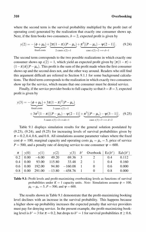
310 Overbooking
where the second term is the survival probability multiplied by the profit (net of
operating cost) generated by the realization that exactly one consumer shows up.
Next, if the firm books two consumers, b = 2, expected profit is given by
y(2) =−(φ + μk)︸ ︷︷ ︸fixed costs
+2π(1−π)(P−μo)︸ ︷︷ ︸2 cases s(2)=1
+π2[(P−μo)−ψ(2−1)]︸ ︷︷ ︸case s(2)=2 =⇒ d=1
. (9.24)
The second term corresponds to the two possible realizations in which exactly one
consumer shows up s(2) = 1, which yield an expected profit given by [π(1−π)+(1−π)π](P−μo). This profit is the sum of the profit made when the first consumer
shows up and the second does not, and the other way around. Readers who still find
this argument difficult are referred to Section 9.1.1 for some background calcula-
tions. The third term corresponds to the realization in which exactly two consumers
show up for the service, which means that one consumer must be denied service.
Finally, if the service provider books to full capacity so that b = B = 3, expected
profit is given by
y(3) =−(φ + μk)︸ ︷︷ ︸fixed costs
+3π(1−π)2(P−μo)︸ ︷︷ ︸3 cases s(3)=1
+3π2(1−π)[(P−μo)−ψ(2−1)]︸ ︷︷ ︸3 cases s(3)=2=⇒ds=1
+π3[(P−μo)−ψ(3−1)]︸ ︷︷ ︸case s(3)=3 =⇒ d=2
. (9.25)
Table 9.1 displays simulation results for the general solution postulated by
(9.23), (9.24), and (9.25) for increasing levels of survival probabilities given by
π = 0.2,0.4,0.6, and 0.8. All simulations assume parameter values where the fixed
cost φ = 100, marginal capacity and operating costs μk = μo = 5, price of service
P = 500, and a penalty rate of denying service to one consumer ψ = 600.
π y(0) y(1) y(2) y(3) b∗ Overbook Es(b∗) Eds(b∗)0.2 0.00 −6.00 49.20 69.36 3 2 0.4 0.112
0.4 0.00 93.00 115.80 33.48 2 1 0.4 0.160
0.6 0.00 192.00 94.80 −160.08 1 0 0.6 0.000
0.8 0.00 291.00 −13.80 −458.76 1 0 0.8 0.000
Table 9.1: Profit levels and profit-maximizing overbooking levels as functions of survival
probabilities under K = 1 capacity units. Note: Simulations assume φ = 100,
μk = μo = 5, P = 500, and ψ = 600.
The results shown in Table 9.1 demonstrate that the profit-maximizing booking
level declines with an increase in the survival probability. This happens because
a higher show-up probability increases the expected penalty that service providers
must pay for denying service. In the present example, the profit-maximizing book-
ing level is b∗= 3 for π = 0.2, but drops to b∗= 1 for survival probabilities π ≥ 0.6.
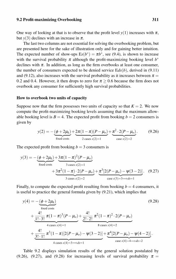
9.2 Profit-maximizing Overbooking 311
One way of looking at that is to observe that the profit level y(1) increases with π ,
but y(3) declines with an increase in π .
The last two columns are not essential for solving the overbooking problem, but
are presented here for the sake of illustration only and for gaining better intuition.
The expected number of show-ups Es(b∗) = πb∗, see (9.4), is shown to increase
with the survival probability π although the profit-maximizing booking level b∗
declines with π . In addition, as long as the firm overbooks at least one consumer,
the number of consumers expected to be denied service Eds(b), derived in (9.11)
and (9.12), also increases with the survival probability as it increases between π =0.2 and 0.4. However, it then drops to zero for π ≥ 0.6 because the firm does not
overbook any consumer for sufficiently high survival probabilities.
How to overbook two units of capacity
Suppose now that the firm possesses two units of capacity so that K = 2. We now
compute the profit-maximizing booking levels assuming that the maximum allow-
able booking level is B = 4. The expected profit from booking b = 2 consumers is
given by
y(2) =−(φ +2μk)︸ ︷︷ ︸fixed costs
+2π(1−π)(P−μo)︸ ︷︷ ︸2 cases s(2)=1
+π2 ·2(P−μo)︸ ︷︷ ︸case s(2)=2
. (9.26)
The expected profit from booking b = 3 consumers is
y(3) =−(φ +2μk)︸ ︷︷ ︸fixed costs
+3π(1−π)2(P−μo)︸ ︷︷ ︸3 cases s(2)=1
+3π2(1−π) ·2(P−μo)︸ ︷︷ ︸3 cases s(2)=2
+π3[2(P−μo)−ψ(3−2)]︸ ︷︷ ︸case s(3)=3=⇒ds=1
. (9.27)
Finally, to compute the expected profit resulting from booking b = 4 consumers, it
is useful to practice the general formula given by (9.21), which implies that
y(4) =−(φ +2μk)︸ ︷︷ ︸fixed costs
(9.28)
+4!
1! ·3!π(1−π)3(P−μo)︸ ︷︷ ︸4 cases s(4)=1
+4!
2! ·2!π2(1−π)2 ·2(P−μo)︸ ︷︷ ︸
8 cases s(4)=2
+4!
3! ·1!π3(1−π)[2(P−μo)−ψ(3−2)]︸ ︷︷ ︸
4 cases s(4)=3=⇒ds=1
+π4[2(P−μo)−ψ(4−2)]︸ ︷︷ ︸case s(4)=4=⇒ds=2
.
Table 9.2 displays simulation results of the general solution postulated by
(9.26), (9.27), and (9.28) for increasing levels of survival probability π =

312 Overbooking
0.2,0.4,0.6, and 0.8. All simulations assume a fixed cost φ = 100, marginal ca-
pacity and operating costs μk = μo = 5, a service price P = 500, and a penalty
rate of denying service to one consumer ψ = 600. Table 9.2 shows results similar
to those in Table 9.1 in the sense that the profitable overbooking level b∗ declines
with an increase in the survival probability π , the expected number of show-ups
Es(b) increases with π , and the expected number of consumers to be denied ser-
vice Eds(b) also increases as long as the firm overbooks at least one consumer.
π y(2) y(3) y(4) b∗ Overbook Es(b∗) Eds(b∗)0.2 88.00 178.24 254.47 4 2 0.8 0.029
0.4 286.00 413.92 457.74 4 2 1.6 0.205
0.6 484.00 544.48 415.74 3 1 1.8 0.216
0.8 682.00 517.36 128.46 2 0 1.6 0.000
Table 9.2: Profit levels and profit-maximizing overbooking levels as functions of survival
probabilities under K = 2 capacity units. Note: Simulations assume φ = 100,
μk = μo = 5, P = 500, and ψ = 600.
9.2.4 Computer algorithm
The computer algorithm described by Algorithm 9.1 runs simple loops over the
booking levels b = 0,K,K + 1, . . . ,B and compares the resulting profit levels y(b)derived from (9.21) and (9.22). This algorithm should first input (using a Read()command, say) the model’s parameters describing K (capacity level), B (maximum
allowable booking level, where B≥ K), φ (fixed cost), μk (marginal capacity cost),
μo (marginal operating cost), P (service’s sale price), ψ (overbooking penalty rate),
and π (survival probability). In addition, the program should include some trivial
loops to ensure that there are no out-of-range (or negative) parameter values.
As for variables, the program should define y[b] (expected profit level given
that b bookings are made) as an array of real numbers of dimension B + 1. The
variable b∗ outputs the profit-maximizing booking level. Inspecting the expected
profit function (9.21) reveals that the “loop” over all possible realizations of the
show-up random variable s(b) is decomposed from two sums: the loop over the
number of show-ups not exceeding capacity (s(b)≤ K) and the loop over show-up
realizations exceeding capacity (s(b) = K +1, . . . ,b). Algorithm 9.1 first computes
the profit y[K] associated with booking exactly to full capacity (b = K). Then, it
runs loops over booking levels exceeding capacity b = K +1, . . . ,B. To summarize,
Algorithm 9.1 compares the profit levels y(0) to y(K) and to every y(b) for b≥K +1, because all booking levels satisfying 1≤ b≤ K−1 cannot be profit maximizing
in this linear model.
Algorithm 9.2 is a continuation of Algorithm 9.1 and summarizes the results
by writing the exact profit-maximizing booking level as well as the corresponding
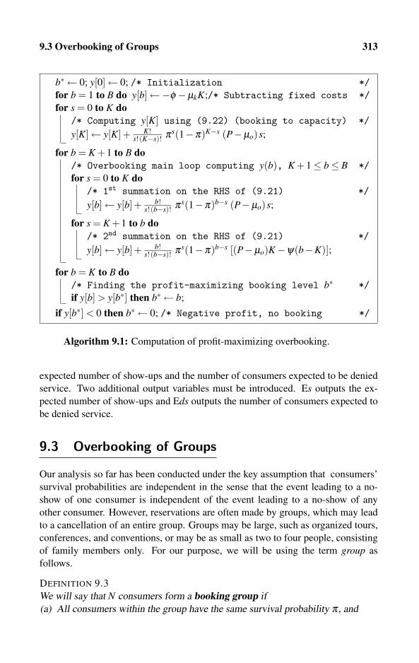
9.3 Overbooking of Groups 313
b∗ ← 0; y[0]← 0; /* Initialization */for b = 1 to B do y[b]←−φ −μkK;/* Subtracting fixed costs */for s = 0 to K do
/* Computing y[K] using (9.22) (booking to capacity) */
y[K]← y[K]+ K!s!(K−s)! πs(1−π)K−s (P−μo)s;
for b = K +1 to B do/* Overbooking main loop computing y(b), K +1≤ b≤ B */for s = 0 to K do
/* 1st summation on the RHS of (9.21) */
y[b]← y[b]+ b!s!(b−s)! πs(1−π)b−s (P−μo)s;
for s = K +1 to b do/* 2nd summation on the RHS of (9.21) */
y[b]← y[b]+ b!s!(b−s)! πs(1−π)b−s [(P−μo)K−ψ(b−K)];
for b = K to B do/* Finding the profit-maximizing booking level b∗ */if y[b] > y[b∗] then b∗ ← b;
if y[b∗] < 0 then b∗ ← 0; /* Negative profit, no booking */
Algorithm 9.1: Computation of profit-maximizing overbooking.
expected number of show-ups and the number of consumers expected to be denied
service. Two additional output variables must be introduced. Es outputs the ex-
pected number of show-ups and Eds outputs the number of consumers expected to
be denied service.
9.3 Overbooking of Groups
Our analysis so far has been conducted under the key assumption that consumers’
survival probabilities are independent in the sense that the event leading to a no-
show of one consumer is independent of the event leading to a no-show of any
other consumer. However, reservations are often made by groups, which may lead
to a cancellation of an entire group. Groups may be large, such as organized tours,
conferences, and conventions, or may be as small as two to four people, consisting
of family members only. For our purpose, we will be using the term group as
follows.
DEFINITION 9.3
We will say that N consumers form a booking group if
(a) All consumers within the group have the same survival probability π , and

314 Overbooking
writeln (“The profit-maximizing refund booking level is ”, b∗,“.”);
Es← π b∗; writeln (Es, “consumers are expected to show up.”);
writeln (“The resulting expected profit level is ”, y[b∗], “.”);
if b∗ = 0 then write (“No booking should be made, cease operation.”);
if b∗ = K then write (“Book exactly to full capacity.”);
if b∗ ≥ K +1 thenwriteln (“Overbook ”, b∗ −K, “consumers.”); Eds← 0;
for s = K +1 to b∗ do/* Computing Eds(b∗) according to (9.12) */
Eds← Eds+ b∗!b∗!(b∗−s)! πs(1−π)b∗−s(s−K);
writeln (Eds, “consumers are expected to be denied service.”);
Algorithm 9.2: Overbooking, the expected number of show-ups, and the
number of consumers expected to be denied service.
(b) Within the group, either all the consumers show up together at the time of
service or the entire group does not show up. Formally, consumers belonging
to the same group are perfectly correlated with respect to their show–no-show
decisions.
A more difficult issue that must be discussed now is how and whether service
can be denied to an entire group. Obviously, this policy issue is decided upon
by the service provider and should be made known to the group before the booking
time. In general, the service provider must make and announce the following policy
decisions.
• Can service be denied to any group of any size?
• Can service be denied to a fraction of consumers within a group, or must it
be denied to the entire group?
• Can service be denied to any group, or should service be denied on a first-
come-first-served basis?
Clearly, the above policy issues should be explicitly stated on the contract or ticket
reserved by the group of customers. For the present analysis, we merely state these
guidelines in the form of assumptions.
ASSUMPTION 9.1
(a) Service can be denied to an entire group of confirmed consumers, but cannot
be denied to a fraction of consumers within a booked group.
(b) Service providers can choose which group is to be denied service so as to max-
imize their profit.

9.3 Overbooking of Groups 315
Assumption 9.1(a) needs no explanation as most groups are formed on the basis
that all group members wish to be served together with their fellow group members.
Assumption 9.1(b) is irrelevant for most of our analysis as we restrict our model to
handle equal-size groups only. However, this assumption becomes important when
groups are of unequal size, because service providers can choose which group to
deny service to based on the group’s relative size.
Each group attempts to book a service that has a total capacity of K consumers
(for all groups together). We make the following assumptions:
ASSUMPTION 9.2
(a) All groups are of equal size and have N consumers.
(b) The size of each booking group is smaller than the service provider’s capacity
level. Formally, N ≤ K.
(c) All groups have an identical survival probability π .
Assumption 9.2(a) is a restriction of our analysis, as it rules out booking of groups
of unequal sizes. Assumption 9.2(b) restricts our analysis to the more common
cases in which a single group cannot consume the entire capacity. For example,
this assumption implies that the tour group is smaller than the aircrafts’ seating
capacity. Assumption 9.2(c) may be justified by the fact that service providers often
cannot distinguish among the types of consumers in each of their booking groups,
so a common survival probability serves as the best approximation. Of course, this
assumption can be tested by looking at real-life rates of group cancellations and
comparing them with the rate of individual cancellations.
Clearly if N = 1, each group consists of a single consumer, in which case the
analysis conducted earlier in Section 9.2 applies. The problem we wish to solve
now is to compute the service provider’s profit-maximizing number of group book-
ings. Thus, the difference between the analysis of this section compared with the
previous sections is that now we allow groups to be of sizes N ≥ 2. This means that
the booking level, to be decided upon by the service provider, should now take the
values of b = 0,N,2N,3N, and so on, instead of b = 0,1,2,3, . . . corresponding to
a group size of N = 1 only.
9.3.1 Simple examples
How to overbook two groups of consumers
Suppose the service provider faces booking requests from two groups, each having
N consumers. Thus, this provider has the option of booking b = 0,N,2N con-
sumers. We continue to assume that y(0) = 0, which means that the fixed and
capacity costs are not borne if the provider ceases operation. If only one group is
booked, there is no overbooking because b = N ≤ K by Assumption 9.2(b). There-
fore, expected profit is given by
y(N) =−φ −μkK +π(P−μo)N, (9.29)

316 Overbooking
which is negative the sum of fixed and capacity costs plus the expected marginal
profit multiplied by the group’s joint survival probability.
Next, when the service provider books two groups, each of size N, expected
profit depends on whether there is an overbooking (2N ≥ K + 1) or underbooking
(2N ≤ K). Therefore, expected profit is given by
y(2N) =−φ −μkK
=
{π2(P−μo)2N +2π(1−π)(P−μo)N if 2N ≤ K[π2 +2π(1−π)](P−μo)N−π2ψN if 2N ≥ K +1.
(9.30)
That is, if 2N ≤ K, the service provider can accommodate the two groups together,
and the resulting profit depends on whether both groups show up, one group shows
up and the other does not (two cases), or neither. In contrast, if 2N ≥ K + 1, the
service provider can accommodate at most N consumers and therefore must deny
service (and pay a penalty) to one group in the event both groups show up (proba-
bility π2).
The decision whether to book two groups, a single group only, or nei-
ther depends on whether y(2N) ≥ max{y(N),0}, y(N) ≥ max{y(2N),0}, or
max{y(2N),y(N)}< 0 = y(0). Comparing (9.30) with (9.29) implies that y(2N)≥y(N) whenever 2N ≤ K. That is, when booking two groups does not result in over-
booking, booking the two groups yields a higher profit than booking one group
only. However, if 2N ≥ K +1,
y(2N)≥ y(N)⇐⇒ ψ ≤ ψ2,1def=
(1−π)(P−μo)π
. (9.31)
Hence, equation (9.31) defines a threshold penalty rate ψ2,1 on denying service,
such that for every penalty rate lower than the threshold level, booking two groups
yields a higher expected profit than booking a single group only.
We conclude the present example with some numerical examples. Consider a
service provider with a given capacity of K = 100 facing booking requests from two
groups of size N = 60. Also let φ = 5000 (fixed cost), μk = μo = 5 (marginal capac-
ity and operating costs), and P = 500 (service’s price). Table 9.3 demonstrates how
the value of the threshold penalty rate ψ2,1 varies with the survival probability pa-
rameter π . Table 9.3 demonstrates at a low survival probability of π = 0.2, booking
θ\π 0.2 0.4 0.6 0.8
ψ2,1 1980.00 742.50 330.00 123.75
ψ3,2 465.88 159.11 60.00 15.47
Table 9.3: Group overbooking: Penalty rate thresholds as functions of survival probabili-
ties Note: Simulations assume K = 100, N = 60, φ = 5000, μk = μo = 5, and
P = 500.
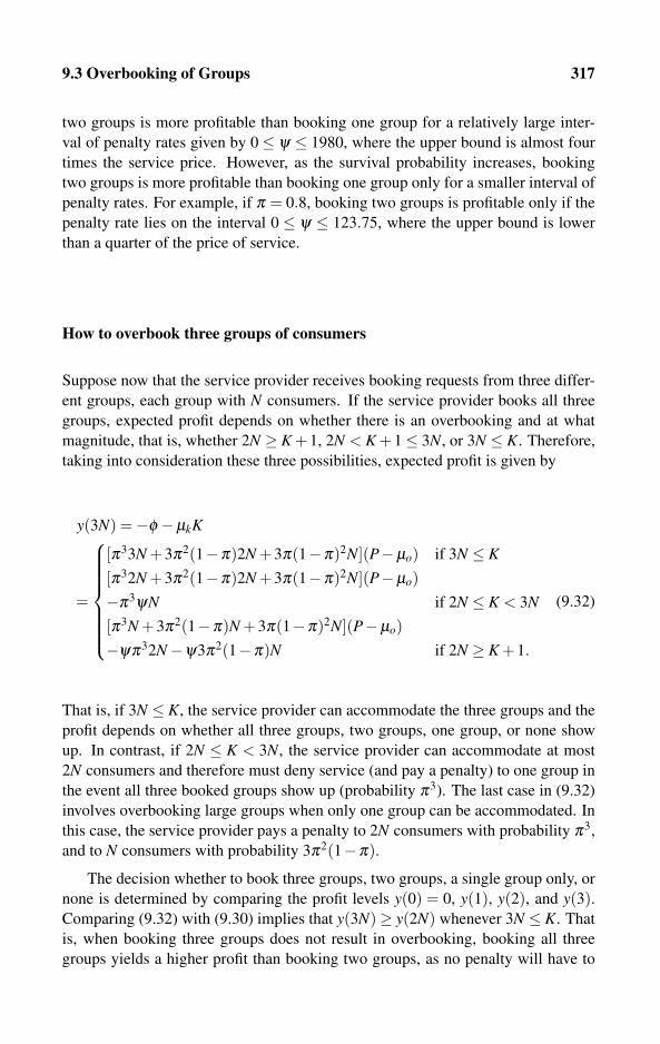
9.3 Overbooking of Groups 317
two groups is more profitable than booking one group for a relatively large inter-
val of penalty rates given by 0≤ ψ ≤ 1980, where the upper bound is almost four
times the service price. However, as the survival probability increases, booking
two groups is more profitable than booking one group only for a smaller interval of
penalty rates. For example, if π = 0.8, booking two groups is profitable only if the
penalty rate lies on the interval 0 ≤ ψ ≤ 123.75, where the upper bound is lower
than a quarter of the price of service.
How to overbook three groups of consumers
Suppose now that the service provider receives booking requests from three differ-
ent groups, each group with N consumers. If the service provider books all three
groups, expected profit depends on whether there is an overbooking and at what
magnitude, that is, whether 2N ≥ K +1, 2N < K +1≤ 3N, or 3N ≤ K. Therefore,
taking into consideration these three possibilities, expected profit is given by
y(3N) =−φ −μkK
=
⎧⎪⎪⎪⎪⎪⎪⎨⎪⎪⎪⎪⎪⎪⎩
[π33N +3π2(1−π)2N +3π(1−π)2N](P−μo) if 3N ≤ K[π32N +3π2(1−π)2N +3π(1−π)2N](P−μo)−π3ψN if 2N ≤ K < 3N[π3N +3π2(1−π)N +3π(1−π)2N](P−μo)−ψπ32N−ψ3π2(1−π)N if 2N ≥ K +1.
(9.32)
That is, if 3N ≤ K, the service provider can accommodate the three groups and the
profit depends on whether all three groups, two groups, one group, or none show
up. In contrast, if 2N ≤ K < 3N, the service provider can accommodate at most
2N consumers and therefore must deny service (and pay a penalty) to one group in
the event all three booked groups show up (probability π3). The last case in (9.32)
involves overbooking large groups when only one group can be accommodated. In
this case, the service provider pays a penalty to 2N consumers with probability π3,
and to N consumers with probability 3π2(1−π).
The decision whether to book three groups, two groups, a single group only, or
none is determined by comparing the profit levels y(0) = 0, y(1), y(2), and y(3).Comparing (9.32) with (9.30) implies that y(3N)≥ y(2N) whenever 3N ≤ K. That
is, when booking three groups does not result in overbooking, booking all three
groups yields a higher profit than booking two groups, as no penalty will have to
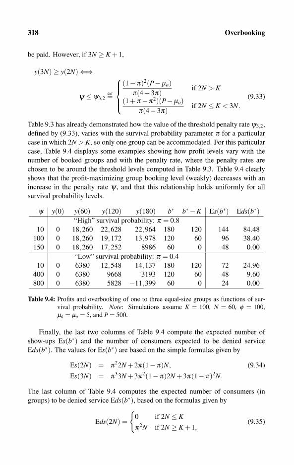
318 Overbooking
be paid. However, if 3N ≥ K +1,
y(3N)≥ y(2N)⇐⇒
ψ ≤ ψ3,2def=
⎧⎪⎪⎨⎪⎪⎩
(1−π)2(P−μo)π(4−3π)
if 2N > K
(1+π−π2)(P−μo)π(4−3π)
if 2N ≤ K < 3N.
(9.33)
Table 9.3 has already demonstrated how the value of the threshold penalty rate ψ3,2,
defined by (9.33), varies with the survival probability parameter π for a particular
case in which 2N > K, so only one group can be accommodated. For this particular
case, Table 9.4 displays some examples showing how profit levels vary with the
number of booked groups and with the penalty rate, where the penalty rates are
chosen to be around the threshold levels computed in Table 9.3. Table 9.4 clearly
shows that the profit-maximizing group booking level (weakly) decreases with an
increase in the penalty rate ψ , and that this relationship holds uniformly for all
survival probability levels.
ψ y(0) y(60) y(120) y(180) b∗ b∗ −K Es(b∗) Eds(b∗)“High” survival probability: π = 0.8
10 0 18,260 22,628 22,964 180 120 144 84.48
100 0 18,260 19,172 13,978 120 60 96 38.40
150 0 18,260 17,252 8986 60 0 48 0.00
“Low” survival probability: π = 0.410 0 6380 12,548 14,137 180 120 72 24.96
400 0 6380 9668 3193 120 60 48 9.60
800 0 6380 5828 −11,399 60 0 24 0.00
Table 9.4: Profits and overbooking of one to three equal-size groups as functions of sur-
vival probability. Note: Simulations assume K = 100, N = 60, φ = 100,
μk = μo = 5, and P = 500.
Finally, the last two columns of Table 9.4 compute the expected number of
show-ups Es(b∗) and the number of consumers expected to be denied service
Eds(b∗). The values for Es(b∗) are based on the simple formulas given by
Es(2N) = π22N +2π(1−π)N, (9.34)
Es(3N) = π33N +3π2(1−π)2N +3π(1−π)2N.
The last column of Table 9.4 computes the expected number of consumers (in
groups) to be denied service Eds(b∗), based on the formulas given by
Eds(2N) =
{0 if 2N ≤ Kπ2N if 2N ≥ K +1,
(9.35)

9.3 Overbooking of Groups 319
because at most one group can be denied service, and
Eds(3N) =
⎧⎪⎨⎪⎩
0 if 3N ≤ Kπ3N if 2N ≥ K < 3Nπ32N +3π2(1−π)N if 2N ≥ K +1.
(9.36)
The second line in (9.36) is for the case in which at most one group may be denied
service, which happens only if all three groups show up. The third line computes
for the case in which at most two groups may be denied service.
9.3.2 General formulation
The examples analyzed in Section 9.3.1 were confined to the booking of two and
three consumer groups only. We now generalize the above formulation to any num-
ber of consumer groups. Recall that the choice variable b denotes the number of
confirmed reservations booked by individual consumers. In a similar way, let gdenote the number of groups of consumers booked by this service provider. There-
fore, b = gN. The task of the service provider is to choose the number of groups to
book to maximize profit, subject to the constraint that the total number of booked
consumers does not exceed the booking limit. Formally, g must be restricted so that
gN ≤ B (or g ≤ B/N), where B is the mandated booking limit, what was assumed
to exceed capacity, B > K.
To be able to separate the computation of profit when the firm overbooks from
the profit when the firm does not overbook, let gK denote the maximum number of
groups that can be booked without exceeding the given capacity level K. Formally,
define
gK def= maxg subject to gN ≤ K. (9.37)
Clearly, if the number of booked groups exceeds capacity, that is, g ≥ gK + 1,
some groups may be denied service, in which case the service provider must pay
large penalties on denying service to groups of consumers. Therefore, if the ser-
vice provider finds it profitable to overbook groups so that g ≥ gK + 1, the profit-
maximizing group booking level must solve
maxg
y(gN) =−φ −μkK +gK
∑i=0
g!
i!(g− i)!π i(1−π)g−i(P−μo)gN
+g
∑i=gK+1
g!
i!(g− i)!π i(1−π)g−i[(P−μo)gKN−ψ(i−gK)N]. (9.38)
The first term is the sum of the fixed and capacity costs. The second term is the
expected revenue net of operating cost resulting from all possible show-ups of igroups out of the gK groups that have confirmed reservations. This sum applies to
all possible group show-ups as long as the total show-ups do not exceed capacity.
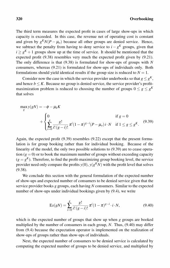
320 Overbooking
The third term measures the expected profit in cases of large show-ups in which
capacity is exceeded. In this case, the revenue net of operating cost is constant
and given by gKN(P− μo) because all other groups are denied service. Hence,
we subtract the penalty from having to deny service to i− gK groups, given that
i ≥ gK + 1 groups show up at the time of service. It should be mentioned that the
expected profit (9.38) resembles very much the expected profit given by (9.21).
The only difference is that (9.38) is formulated for show-ups of groups with Nconsumers, whereas (9.21) is formulated for show-ups of individuals only. Both
formulations should yield identical results if the group size is reduced to N = 1.
Consider now the case in which the service provider underbooks so that g≤ gK ,
and hence b≤ K. Because no group is denied service, the service provider’s profit-
maximization problem is reduced to choosing the number of groups 0 ≤ g ≤ gK
that solves
maxg
y(gN) =−φ −μkK
+
⎧⎪⎨⎪⎩
0 if g = 0g
∑i=0
g!
i!(g− i)!π i(1−π)g−i(P−μo) i ·N if 1≤ g≤ gK .
(9.39)
Again, the expected profit (9.39) resembles (9.22) except that the present formu-
lation is for group booking rather than for individual booking. Because of the
linearity of the model, the only two possible solutions to (9.39) are to cease opera-
tion (g = 0) or to book the maximum number of groups without exceeding capacity
(g = gK). Therefore, to find the profit-maximizing group booking level, the service
provider need only compare the profits y(0), y(gKN) with the profit level that solves
(9.38).
We conclude this section with the general formulation of the expected number
of show-ups and expected number of consumers to be denied service given that the
service provider books g groups, each having N consumers. Similar to the expected
number of show-ups under individual bookings given by (9.4), we write
Es(gN) =g
∑i=0
g!
i!(g− i)!π i(1−π)g−i · i ·N, (9.40)
which is the expected number of groups that show up when g groups are booked
multiplied by the number of consumers in each group, N. Thus, (9.40) may differ
from (9.4) because the expectation operator is implemented on the realization of
show-ups of groups rather than show-ups of individuals.
Next, the expected number of consumers to be denied service is calculated by
computing the expected number of groups to be denied service, and multiplied by
9.3 Overbooking of Groups 321
the number of consumers in each group, N. Therefore,
Eds(gN) = ⎧⎪⎨⎪⎩
0 if g≤ gK
g
∑i=gK+1
g!
i!(g− i)!π i(1−π)g−i(i−gK)N if g≥ gK +1.
(9.41)
The expected number of consumers to be denied service given by (9.41) is some-
what different from that of overbooking of individuals given by (9.12), because
under group overbooking, a denial of service is likely to result in some underuti-
lization of capacity. That is, in the event the service provider must deny service
to some groups, the number of served consumers becomes gKN, which could be
strictly below the capacity level K. In other words, because booking and service
denial are restricted to “chunks” of consumers in the form of groups, it may happen
that capacity will remain underused even if the firm overbooks. To see this, con-
sider the following example: Suppose capacity is K = 100, and that each group has
N = 60 consumers. Even if the firm books two groups so that b = 120 > 100 = K,
if both groups show up, the firm must deny service to 60 consumers, leading to an
underutilization of capacity of 40 consumers. Obviously, this underutilization can-
not occur with overbooking of individuals because denying service to individuals
still leaves K consumers to be served.
9.3.3 Computer algorithm
The computer algorithm we now derive is a slight modification of Algorithm 9.1 to
accommodate booking groups (instead of booking individual consumers). There-
fore, the reader is referred to Section 9.2.4 for the list and description of all the
parameters that the program should input and the variables that should be defined.
In addition to this list, the present algorithm should input N (using a Read() com-
mand, say), which is the number of consumers in each group. The only new vari-
able that we now introduce is gB, which is the maximum number of groups (of
size N) that can be booked without exceeding the mandated booking limit B. The
following algorithm computes this group booking limit by solving gB def= maxg,
subject to gN ≤ B.
As with Algorithm 9.1, Algorithm 9.3 first computes y[gKN], which is the ex-
pected profit when g = gK (booking as close as possible to full capacity without
overbooking). Then, it computes the expected profit y[gN] for all booking levels
gK + 1 ≤ g ≤ gB associated with overbooking. To summarize, similar to Algo-
rithm 9.1, Algorithm 9.3 compares the profit levels y(0) with y(gKN) and every
y(gN) for g≥ gK +1 that solve (9.38) because all other group booking levels (sat-
isfying 1≤ g≤ gK−1) cannot be profit maximizing in this linear model.
Algorithm 9.4 is a continuation of Algorithm 9.3 and summarizes the results
by writing the exact profit-maximizing group booking level as well as the corre-

322 Overbooking
gK ← 0; gB← 0; g∗ ← 0; /* Initialization */repeat gK ← gK +1 until (gK +1)N > K; /* Computing gK */repeat gB← gB +1 until (gB +1)N > B; /* Computing gB */for g = 1 to gB do y[gN]←−φ −μkK; /* Fixed costs */for i = 0 to gK do
/* Computing y[gKN] using (9.39) (no overbooking) */
y[gKN]← y[gKN]+ gK !i!(gK−i)! π i(1−π)gK−i (P−μo) i ·N;
for g = gK +1 to gB do/* Overbooking loop computing y(gN), gK +1≤ g≤ gB */for i = 0 to gK do
/* 1st summation in (9.38) */
y[gN]← y[gN]+ g!i!(g−i)! π i(1−π)g−i (P−μo) i ·N;
for i = gK +1 to g do/* 2nd summation in (9.38) */
y[gN]← y[gN]+ g!i!(g−i)! π i(1−π)g−i [(P−μo)gK−ψ(i−gK)]N;
for g = gK to gB do/* Finding the profit-maximizing booking level g∗ */if y[gN] > y[g∗N] then g∗ ← g;
if y[g∗N] < 0 then g∗ ← 0; /* Negative profit, no booking */
Algorithm 9.3: Computation of profit-maximizing group overbooking.
sponding expected number of show-ups and the number of consumers expected to
be denied service.
9.4 Exercises
1. Use the binomial distribution formula given by (9.3) to compute the following
probabilities.
(a) The probability that exactly two consumers show up out of three confirmed
reservations, Pr{s(3) = 2}. Compare your answer with the result given
by (9.2). Show your entire derivation.
(b) Solve the previous problem assuming that the survival probability is π =0.8.
(c) The probability that exactly 52 passengers will show up for a flight with 55
confirmed reservations, Pr{s(55) = 52}.

9.4 Exercises 323
write (“The profitable booking level consists of ”, g∗,“groups,”);
writeln (“or equivalently, booking ”, g∗N,“consumers.”);
writeln (“The resulting expected profit level is ”, y[g∗N], “.”);
if g∗ = 0 then write (“No bookings should be made, cease operation.”);
if g∗ = gK then write (“Book as close to full capacity as possible.”);
if g∗ ≥ gK +1 thenwrite (“Overbook ”, g∗ −gK , “groups.”);
writeln (“or equivalently, overbook ”, (g∗ −gK)N,“consumers.”);
Es← 0; /* Computing Es(g∗N) according to (9.40) */for i = 0 to g∗ do
Es← Es+ g∗!i!(g∗−i)! π i(1−π)g∗−i · i ·N;
writeln (Es, “consumers are expected to show up.”);
Eds← 0; /* Computing Eds(g∗N) according to (9.41) */for i = gK +1 to gB do
Eds← Eds+ g∗!i!(g∗−i)! π i(1−π)g∗−i(i−gK)N;
writeln (Eds, “consumers are expected to be denied service.”);
Algorithm 9.4: Group overbooking, the expected number of show-ups, and
the number of consumers expected to be denied service.
(d) Solve the previous problem assuming that the survival probability is π =0.9.
(e) Using the formula given by (9.4), compute the expected number of show-
ups given that the survival probability is π = 0.7 and b = 52 have been
booked.
2. Suppose a service provider books b = 5 consumers for a service with a capacity
of K = 3. Each consumer has an independent survival probability given by
π = 0.8. Using the set of examples given by equation (9.6), do the following
calculations and show your derivations.
(a) Compute the probability that exactly one consumer is denied service. For-
mally, compute Pr{ds(5) = 1}.(b) Compute the probability that exactly two consumers are denied service. For-
mally, compute Pr{ds(5) = 2}.(c) Compute the probability that at least one consumer is denied service. For-
mally, compute Pr{ds(5)≥ 1}.(d) Compute the probability that no consumer is denied service, using the method
described by equation (9.8).

324 Overbooking
(e) Compute the probability that no consumer is denied service, using the method
described by equation (9.10).
(f) Using equation (9.11), compute the expected number of consumers to be
denied service, Eds(5).
3. Suppose you are the CEO of a firm endowed with K = 3 units of capacity. The
maximum allowable booking level is B = 4. That is, your firm has the option
of overbooking at most one consumer. In this exercise, you will have to decide
how many consumers to book similar to the analysis given in Section 9.2.3. Do
the following calculations.
(a) Formulate the expected profit function y(3) assuming that your firm books
exactly b = 3 consumers.
(b) Formulate the expected profit function y(4) assuming that your firm books
exactly b = 4 consumers.
(c) Using the above computations, compute the profit-maximizing booking level
assuming that the observed parameter values are φ = 0 (fixed cost), μk =μo = 10 (marginal capacity and operating cost), P = 500 (service’s price),
ψ = 3430 (overbooking penalty rate), and π = 0.5 (survival probability).
4. You are now in charge of BUMPME, an airline that provides regular service
for passengers vacationing on a remote African island. Your airline books only
groups of 40 passengers each and operates an aircraft with a seating capacity of
100 passengers. The regulator prohibits the airline from booking more than 200
passengers. Using the analysis of Section 9.3, solve the following problems.
(a) Formulate the expected profit function y(80) assuming that your firm books
exactly g = 2 groups.
(b) Formulate the expected profit function y(120) assuming that your firm books
exactly g = 3 groups.
(c) Using your answers to (a) and (b), compute the penalty rate ψ that would
make BUMPME indifferent between booking two and three groups, assum-
ing that the observed parameter values are φ = 1000 (fixed cost), μk = μo =10 (marginal capacity and operating costs), P = 500 (service’s price), and
π = 0.8 (survival probability). Explain how many groups should be booked
if the actual penalty rate is above ψ and below it.
Chapter 10
Quality, Loyalty, Auctions, and Advertising
10.1 Quality Differentiation and Classes 32610.1.1 Preferences for quality: Classifications and assumptions
10.1.2 Selecting the profit-maximizing quality level
10.1.3 Computer algorithm for a single-quality choice
10.1.4 Selecting multiple quality levels
10.2 Damaged Goods 33210.3 More on Pricing under Competition 335
10.3.1 Behavior-based pricing
10.3.2 Price matching
10.4 Auctions 34310.4.1 Open English and sealed-bid second-price auctions
10.4.2 Open Dutch and sealed-bid first-price auctions
10.4.3 Revenue equivalence under independent valuations
10.5 Advertising Expenditure 35210.5.1 Demand functions and advertising
10.5.2 Profit-maximizing advertising expenditure
10.6 Exercises 355
This chapter analyzes some additional pricing techniques and marketing tactics
intended to further enhance sellers’ profits. Section 10.1 links pricing decisions
to innovation and product design decisions by computing the profit-maximizing
quality levels and service classes to be introduced into the market. The underlining
assumption in this analysis is that sellers cannot directly price discriminate among
the different consumer groups. Therefore, the seller must devise a price scheme
under which consumers belonging to different consumer groups choose to purchase
different quality levels.
Section 10.2 examines a special case of the above problem by analyzing mar-
kets in which the seller may find it profitable to sell a “damaged good” (such as
a version containing less features) to consumers with low willingness to pay, to
326 Quality, Loyalty, Auctions, and Advertising
segment the market between consumers with high and low willingness to pay. The
interesting feature of this result is that the low-quality product is more costly to pro-
duce than the high-quality product. In the case of a service, the low-quality service
is more costly to deliver than the original undamaged high-quality service.
Section 10.3.1 analyzes repeatedly purchased services and identifies the con-
ditions under which a firm should provide a discount to its returning “loyal” con-
sumers, and also the conditions for the polar case under which the firm should dis-
count the price for consumers who switch from competing brands. Section 10.3.2
explores the consequences of having sellers commit to matching the prices offered
by competing sellers, and demonstrates why this strategy can be profit enhancing.
Section 10.4 analyzes auctions. The major advantage of using auctions over price
setting is that under auctions, price offers are made by the buyers and not by the
seller. Section 10.5 concludes with the analysis of profit-maximizing investment in
advertising.
10.1 Quality Differentiation and Classes
As far back as the 19th century, the French economist Dupuit realized that the pro-
vision of different qualities of service (different classes) could be profit enhancing.
In his words,
It is not because of the few thousand francs which would have to be
spent to put a roof over the third-class carriage ... What the company
is trying to do is prevent the passengers who can pay the second-class
fare from traveling third class.
—E. Dupuit (Ekelund 1970)
Differentiating a product or a service according to quality enables the seller to
price discriminate between those who have high willingness to pay for the prod-
uct/service and those who have low willingness to pay. Otherwise, as a direct
consequence of the “law of one price,” if identical products or services are sold at
different prices, no consumer would be willing to pay the high price. By either
enhancing the quality of the upper-end product or damaging the quality of the low-
end product, the seller can induce consumers with high willingness to pay to buy
the upper-end product that is sold at a higher price. This is the essence of market
segmentation.
The subject analyzed in this section is of utmost importance to firms racing to
innovate new products and services, and for firms upgrading the quality of already-
marketed products, because it manifests the tight relationship between engineering-
based decisions and marketing decisions. Basically this means that marketing peo-
ple in charge of pricing decisions should inform product engineers and product de-
signers about consumers’ willingness to pay for the different quality levels, whereas
10.1 Quality Differentiation and Classes 327
engineers should be communicating with the marketing people on the types of prod-
uct and service quality levels the firm may be able to supply. In fact, the success of
such firms depends on proper communication between these two different bodies
within the same firm.
Technically speaking, the analysis in this section focuses on pricing tactics the
seller should employ when consumers with high willingness to pay cannot be di-
rectly distinguished from consumers with low willingness to pay. As we have
already discussed in Section 1.2.3, offering consumers a “proper” list of quality-
dependent prices can induce different types of consumers to purchase different
quality levels, thereby indirectly revealing their type to the seller. By “proper”
pricing, we mean that the seller must address the following two major questions:
(a) Which and how many different quality levels should be introduced into the
market?
(b) How should the different quality levels be priced so that different consumer
types choose to buy different quality levels?
10.1.1 Preferences for quality: Classifications and assumptions
The main variable notation for this section is as follows: The set of all possible
quality levels is denoted by B. For example, many software companies sell three
versions of the same software, and name these versions “Pro,” “Standard,” and
“Basic.” In this example, B = {Pro,Standard,Basic}. In general, let the index
i∈B denote a possible quality level, where we often write i∈B = {A,B,C, . . . ,Z},or i ∈B = {1,2,3,4}, and so forth. The firm’s unit production or service-delivery
cost of quality i is denoted by μi, for every product or service with quality i ∈B.
There are M consumer types indexed by �, � = 1,2, . . . ,M. In view of Table 1.4,
which summarizes the notation used throughout this book, V i� denotes a type �
consumer’s maximum willingness to pay for a quality i product, where i ∈B. N�
denotes the number of consumers who are of type �.
The analysis of quality (as opposed to other types of service differentiation)
means that all consumers “tend to agree” how to rank the service levels. There-
fore, the following assumption is needed for interpreting service differentiation as
quality differentiation:
ASSUMPTION 10.1
Services and products with different qualities are vertically differentiated. For-
mally, V A� ≥V B
� ≥ ·· · ≥V Z� , for each consumer type � = 1, . . . ,M.
Basically, Assumption 10.1 implies all potential consumers, regardless of their
type, are willing to pay more for quality A than for quality B, and more for quality Bthan for quality C, and so on. However, note that Assumption 10.1 does not imply
that all consumers have equal willingness to pay for each service quality.
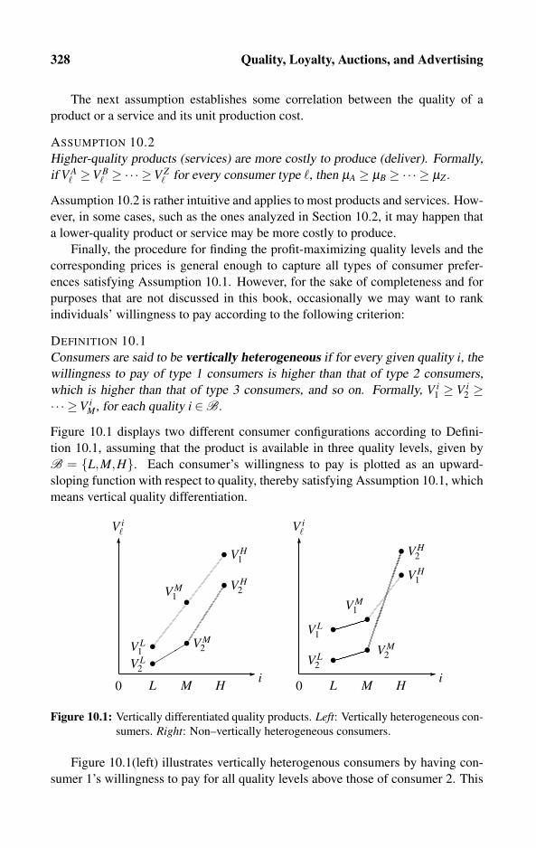
328 Quality, Loyalty, Auctions, and Advertising
The next assumption establishes some correlation between the quality of a
product or a service and its unit production cost.
ASSUMPTION 10.2
Higher-quality products (services) are more costly to produce (deliver). Formally,
if V A� ≥V B
� ≥ ·· · ≥V Z� for every consumer type �, then μA ≥ μB ≥ ·· · ≥ μZ .
Assumption 10.2 is rather intuitive and applies to most products and services. How-
ever, in some cases, such as the ones analyzed in Section 10.2, it may happen that
a lower-quality product or service may be more costly to produce.
Finally, the procedure for finding the profit-maximizing quality levels and the
corresponding prices is general enough to capture all types of consumer prefer-
ences satisfying Assumption 10.1. However, for the sake of completeness and for
purposes that are not discussed in this book, occasionally we may want to rank
individuals’ willingness to pay according to the following criterion:
DEFINITION 10.1
Consumers are said to be vertically heterogeneous if for every given quality i, the
willingness to pay of type 1 consumers is higher than that of type 2 consumers,
which is higher than that of type 3 consumers, and so on. Formally, V i1 ≥ V i
2 ≥·· · ≥V i
M, for each quality i ∈B.
Figure 10.1 displays two different consumer configurations according to Defini-
tion 10.1, assuming that the product is available in three quality levels, given by
B = {L,M,H}. Each consumer’s willingness to pay is plotted as an upward-
sloping function with respect to quality, thereby satisfying Assumption 10.1, which
means vertical quality differentiation.
�
0 L M H� i
���•
••
•
• V H1
V H2
V L2
V L1
V M2
V M1
•
�
0 L M H� i
••
•
••
•
V H1
V H2
V M2
V M1
V L1
V L2
V i� V i
�
Figure 10.1: Vertically differentiated quality products. Left: Vertically heterogeneous con-
sumers. Right: Non–vertically heterogeneous consumers.
Figure 10.1(left) illustrates vertically heterogenous consumers by having con-
sumer 1’s willingness to pay for all quality levels above those of consumer 2. This
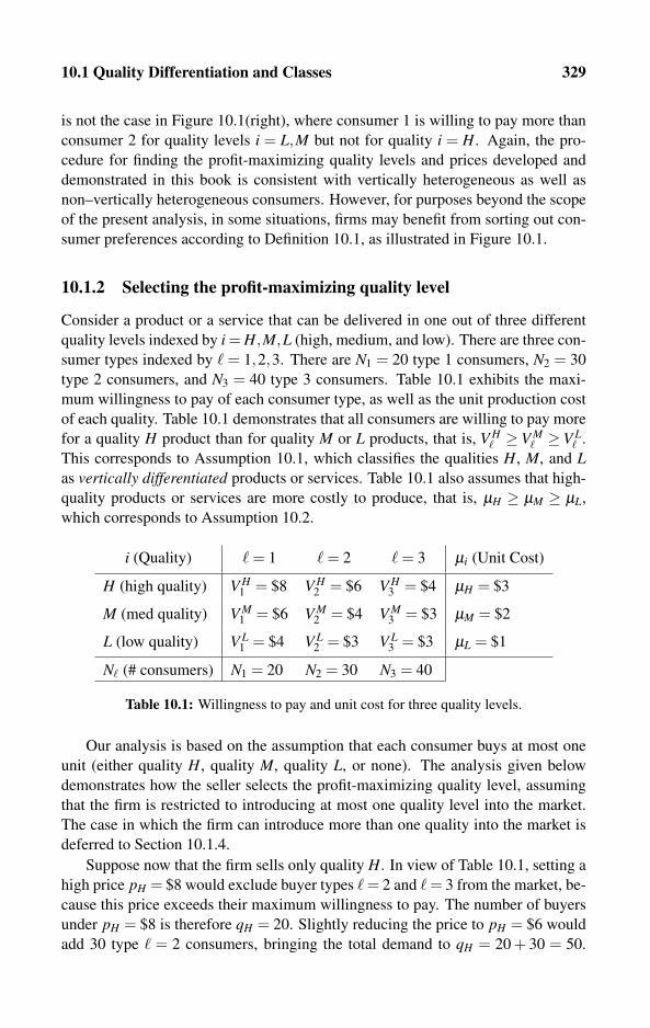
10.1 Quality Differentiation and Classes 329
is not the case in Figure 10.1(right), where consumer 1 is willing to pay more than
consumer 2 for quality levels i = L,M but not for quality i = H. Again, the pro-
cedure for finding the profit-maximizing quality levels and prices developed and
demonstrated in this book is consistent with vertically heterogeneous as well as
non–vertically heterogeneous consumers. However, for purposes beyond the scope
of the present analysis, in some situations, firms may benefit from sorting out con-
sumer preferences according to Definition 10.1, as illustrated in Figure 10.1.
10.1.2 Selecting the profit-maximizing quality level
Consider a product or a service that can be delivered in one out of three different
quality levels indexed by i = H,M,L (high, medium, and low). There are three con-
sumer types indexed by � = 1,2,3. There are N1 = 20 type 1 consumers, N2 = 30
type 2 consumers, and N3 = 40 type 3 consumers. Table 10.1 exhibits the maxi-
mum willingness to pay of each consumer type, as well as the unit production cost
of each quality. Table 10.1 demonstrates that all consumers are willing to pay more
for a quality H product than for quality M or L products, that is, V H� ≥ V M
� ≥ V L� .
This corresponds to Assumption 10.1, which classifies the qualities H, M, and Las vertically differentiated products or services. Table 10.1 also assumes that high-
quality products or services are more costly to produce, that is, μH ≥ μM ≥ μL,
which corresponds to Assumption 10.2.
i (Quality) � = 1 � = 2 � = 3 μi (Unit Cost)
H (high quality) V H1 = $8 V H
2 = $6 V H3 = $4 μH = $3
M (med quality) V M1 = $6 V M
2 = $4 V M3 = $3 μM = $2
L (low quality) V L1 = $4 V L
2 = $3 V L3 = $3 μL = $1
N� (# consumers) N1 = 20 N2 = 30 N3 = 40
Table 10.1: Willingness to pay and unit cost for three quality levels.
Our analysis is based on the assumption that each consumer buys at most one
unit (either quality H, quality M, quality L, or none). The analysis given below
demonstrates how the seller selects the profit-maximizing quality level, assuming
that the firm is restricted to introducing at most one quality level into the market.
The case in which the firm can introduce more than one quality into the market is
deferred to Section 10.1.4.
Suppose now that the firm sells only quality H. In view of Table 10.1, setting a
high price pH = $8 would exclude buyer types � = 2 and � = 3 from the market, be-
cause this price exceeds their maximum willingness to pay. The number of buyers
under pH = $8 is therefore qH = 20. Slightly reducing the price to pH = $6 would
add 30 type � = 2 consumers, bringing the total demand to qH = 20 + 30 = 50.

330 Quality, Loyalty, Auctions, and Advertising
Finally, lowering the price to pH = $4 would induce all consumers to buy the qual-
ity H good so that the sales level becomes qH = 20 + 30 + 40 = 90 units. Clearly,
the seller cannot enhance profit by any further reduction in price as the entire mar-
ket is already served under pH = $4. The profit levels corresponding to the above
three prices are therefore given by
yH =
⎧⎪⎨⎪⎩
20(8−3)−φ = $100−φ if pH = $8
50(6−3)−φ = $150−φ if pH = $6
90(4−3)−φ = $90−φ if pH = $4,
(10.1)
where φ ≥ 0 is the firm’s fixed cost. Next, the profit when only quality M is intro-
duced into the market is
yM =
⎧⎪⎨⎪⎩
20(6−2)−φ = $80−φ if pM = $6
50(4−2)−φ = $100−φ if pM = $4
90(3−2)−φ = $90−φ if pM = $3.
(10.2)
Similarly, the profit when only quality L is introduced into the market is
yL =
{20(4−1)−φ = $60−φ if pL = $4
90(3−1)−φ = $180−φ if pL = $3.(10.3)
Comparing (10.1), (10.2), and (10.3) reveals that the seller maximizes profit by
introducing quality L into the market for the price of pL = $3, thereby making the
product “affordable” to all consumer types. The resulting profit is y = $180−φ .
10.1.3 Computer algorithm for a single-quality choice
The examples given above hint at the general method for how to determine the
profit-maximizing quality level to be introduced into the market and how to price
it. Algorithm 10.1 computes the profit-maximizing quality level, the corresponding
price, and the resulting profit level.
The program should input the following parameters: the set B listing all possi-
ble quality levels (such as H, M, and L as in the previous examples) and the number
of consumer types M. Consumers’ maximum willingness to pay should be input
into a nonnegative array of real numbers V [�, i] reflecting type �’s maximum will-
ingness to pay (valuation) for a quality level i, i ∈B and � = 1, . . . ,M. The number
of consumers of each type should be input into an M-dimensional array of natural
numbers N[�], � = 1, . . . ,M. The program should also input the seller’s unit costs
of producing each quality μ[i], i ∈B, and the fixed cost φ .
As for output variables, Algorithm 10.1 stores the profit-maximizing quality
choice on imax. For all quality levels, i ∈B (not only for imax), pmax[i] is a nonneg-
ative array of real variables that records the profit-maximizing price when quality

10.1 Quality Differentiation and Classes 331
ymax← 0; for i ∈B do ymax[i]← 0; /* Initialization */for i ∈B do
/* Main loop over all possible quality levels */for � = 1 to M do
p[i]←V [�, i]; q[i]← 0; /* Set price for i to equal �’svaluation, check who else buys at this price */
for � = 1 to M doif p[i]≤V [�, i] then q[i]← q[i]+N[i]; /* Add buyers */y[i]← q[i](p[i]−μ[i]); /* Store temporary profit */
if ymax[i] < y[i] then/* New profit-max price for quality i found */pmax[i]← p[i]; qmax[i]← q[i]; ymax[i]← y[i];
if ymax < ymax[i] thenimax← i; ymax← ymax[i]; /* New profit-max i found */
for i ∈B do ymax[i]← ymax[i]−φ ; /* Subtract fixed cost */writeln (“The seller should introduce quality”, imax, “Total profit is ymax =”,
ymax[imax], “The number of buyers is”, q[imax] );
for i ∈B do writeln (“If quality”, i, “is selected instead of”, imax, “it
should be priced at”, pmax[i], “sales and profit would be”, qmax[i], and,
ymax[i]); /* If other qualities are selected instead */
Algorithm 10.1: Selecting the profit-maximizing quality level.
i is introduced, and qmax[i] and ymax[i] the corresponding sales and profit levels. In
addition to writing the profit-maximizing quality level the seller should choose to
introduce into the market, the program also writes what should be the price for each
other quality level i if the seller chooses to introduce it instead of imax.
10.1.4 Selecting multiple quality levels
Sections 10.1.2 and 10.1.3 restricted the seller’s decision to selecting at most one
quality level out of multiple quality levels the firm is capable of producing (or
delivering, in case of a service). However, often, as this section demonstrates, the
firm may be able to further enhance its profit by offering to consumers a variety of
quality levels from which to choose. The difficulty with offering multiple quality
levels to heterogenous consumers is in computing a price for each quality level so
that not all consumers end up buying the same quality level. That is, the “trick”
here is to find a vector of prices (price for each quality) so that the market will
be segmented in the sense that consumers with relatively high valuations for high-
332 Quality, Loyalty, Auctions, and Advertising
quality goods buy high-quality goods, whereas all other consumers buy goods with
lower qualities.
To demonstrate the difficulty in finding the profit-maximizing prices that seg-
ment the market among the different consumer types, let us reexamine Table 10.1,
in which we have shown that if the seller is restricted to selecting at most one quality
level, the profit-maximizing choice would be to introduce quality L into the market
and sell it for the price pL = $3, under which all consumer types would buy it. A
closer examination of Table 10.1 reveals that type � = 1 consumers are willing to
pay a high price pH = $8 for a high-quality good. However, if the seller introduces
quality H as a second quality and prices it at pH = $8, no consumer would choose
to buy it. To see this, Table 10.1 implies that the net gain to type 1 consumers from
buying H is V H1 − pH = 8−8 < 4−3 = V L
1 − pL, hence they will choose to buy L.
For type 2 consumers, V H2 − pH = 6−8 < 3−3 = 0 = V L
2 − pL, and the same for
type 3 consumers. Therefore, introducing quality H for the price pH = $8 will not
be successful.
The above discussion hints that the seller must reduce pH to induce type 1
consumers to purchase quality H instead of L. Formally, the maximum price for Hthat would induce type 1 consumers to buy H instead of L is determined from
V H1 − pH = 8− pH ≥ V L
1 − pL = 4− 3, yielding pH = $7. Clearly, type 2 and 3
consumers will choose to buy L because V H2 − pH = 6− 7 < 0 ≤ V L
2 − pL and
V H3 − pH = 4−7 < 0≤V L
3 − pL. Therefore, under the prices pH = $7 and pL = $3,
the market is segmented; however, it remains to check whether this segmentation
is more profitable than selling one quality only. In view of Table 10.1, the profit
under these prices is
yH,L = 20(7−3)+(30+40)(3−1) = $220−φ > $180−φ = yL, (10.4)
where φ is the firm’s fixed cost and yL is the profit when the firm sells quality L only,
which was computed in (10.3). Thus, this market segmentation is profit enhancing
relative to selling a single quality only.
10.2 Damaged Goods
Perhaps the most interesting pricing technique related to quality classes is that of
damaged goods. Here, manufacturers intentionally damage some features of a good
or a service to be able to price discriminate among the consumer groups. A proper
implementation of this technique may even generate a Pareto improvement, which
is a situation in which the seller and all buyers are better off compared with the allo-
cation in which only the original undamaged quality is sold. The most paradoxical
consequence of this technique is that the good that is more costly to produce (the
damaged good) is sold for a lower price as it has a lower quality. Deneckere and
McAfee (1996) and Shapiro and Varian (1999) list a wide variety of industries in
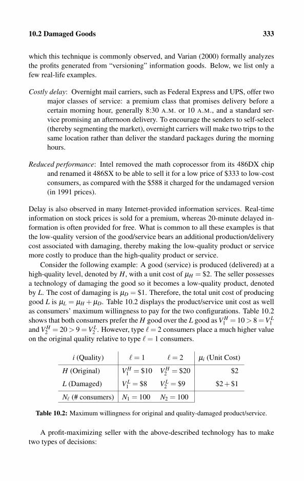
10.2 Damaged Goods 333
which this technique is commonly observed, and Varian (2000) formally analyzes
the profits generated from “versioning” information goods. Below, we list only a
few real-life examples.
Costly delay: Overnight mail carriers, such as Federal Express and UPS, offer two
major classes of service: a premium class that promises delivery before a
certain morning hour, generally 8:30 A.M. or 10 A.M., and a standard ser-
vice promising an afternoon delivery. To encourage the senders to self-select
(thereby segmenting the market), overnight carriers will make two trips to the
same location rather than deliver the standard packages during the morning
hours.
Reduced performance: Intel removed the math coprocessor from its 486DX chip
and renamed it 486SX to be able to sell it for a low price of $333 to low-cost
consumers, as compared with the $588 it charged for the undamaged version
(in 1991 prices).
Delay is also observed in many Internet-provided information services. Real-time
information on stock prices is sold for a premium, whereas 20-minute delayed in-
formation is often provided for free. What is common to all these examples is that
the low-quality version of the good/service bears an additional production/delivery
cost associated with damaging, thereby making the low-quality product or service
more costly to produce than the high-quality product or service.
Consider the following example: A good (service) is produced (delivered) at a
high-quality level, denoted by H, with a unit cost of μH = $2. The seller possesses
a technology of damaging the good so it becomes a low-quality product, denoted
by L. The cost of damaging is μD = $1. Therefore, the total unit cost of producing
good L is μL = μH + μD. Table 10.2 displays the product/service unit cost as well
as consumers’ maximum willingness to pay for the two configurations. Table 10.2
shows that both consumers prefer the H good over the L good as V H1 = 10 > 8 =V L
1
and V H2 = 20 > 9 = V L
2 . However, type � = 2 consumers place a much higher value
on the original quality relative to type � = 1 consumers.
i (Quality) � = 1 � = 2 μi (Unit Cost)
H (Original) V H1 = $10 V H
2 = $20 $2
L (Damaged) V L1 = $8 V L
2 = $9 $2+$1
N� (# consumers) N1 = 100 N2 = 100
Table 10.2: Maximum willingness for original and quality-damaged product/service.
A profit-maximizing seller with the above-described technology has to make
two types of decisions:

334 Quality, Loyalty, Auctions, and Advertising
Design: Whether or not to introduce a quality-damaged product/service into the
market, given that the damaged version requires an additional per-unit cost.
Marketing: How to price the two different qualities when introduced into the mar-
ket.
In the present example, the seller decides whether to offer quality H (original), L(purposely damaged), or both, and the price of each quality, pH and pL, if both qual-
ities are introduced. Clearly, because all consumers prefer H over L and because His less costly to produce than L, it is not profitable to sell only L (the damaged good)
to both consumers. Therefore, the seller is left to consider the following remaining
options:
Selling H to type 2 consumers only: This is accomplished by not introducing a dam-
aged version and by setting a sufficiently high price, pH = $20, under which
consumer � = 1 will not buy. The resulting profit is y = 100(20− 2)−φ =$1800−φ , where φ ≥ 0 is the firm’s fixed cost.
Selling H to both consumer types: Again, selling only the original high-quality
good but at a much lower price, pH = $10, to induce consumer � = 1 to
buy. The resulting profit is y = (100+100)(10−2)−φ = $1600−φ .
Selling H to type 2, and L to type 1 consumers: Introducing the damaged good into
the market. Consumer 2 will choose H over L if V H2 − pH ≥V L
2 − pL. Thus,
the seller must set pH ≤ V H2 −V L
2 + pL = 11 + pL. To induce type 1 con-
sumers to buy the damaged good L, the seller should set pL = $8, which
implies that pH = 11 + 8 = $19. Total profit is therefore y = 100(19−2)+100(8−2−1)−φ = $22,000−φ .
Clearly, the third option is the profit-maximizing strategy for the example displayed
in Table 10.2.
Perhaps the most striking feature of the last pricing scheme (selling H to type 2
and L to type 1) is that no one is worse off compared with the second most profitable
strategy (selling only H to type 2 only). Under the first option, consumer 2 pays
pH = $20, thereby excluding all type 1 consumers. However, the introduction of
the damaged good L lowers the price of the H good to pH = 19, thereby increasing
the welfare of type 2 consumers. In addition, the seller’s profit is enhanced to
y = $22,000−φ from y = $18,000−φ . Type 1 consumers remain indifferent, but
it is possible to reduce pL and pH by a few cents to make even type 1 consumers
strictly better off when the damaged good is introduced.
Figure 10.2 illustrates buyers’ decisions on which quality to purchase in the
pL–pH space. The parallelogram at the center consists of all price pairs pL and pH
under which the market is segmented in the sense that type � = 1 consumers choose
to purchase L (the damaged good), whereas type � = 2 consumers choose to buy
H (original quality). In this range, V L1 − pL ≥ V H
1 − pH and V H2 − pH ≥ V L
2 − pL.

10.3 More on Pricing under Competition 335
�
�
pL
$19
V L1 = $8
pH0
�����������
�����������
pL = pH −11pL = pH −1
$1 $9 $11
type 1 buys H type 1 buys L
type 2 buys H type 2 buys L
Segmented market
•
$20
••
V L2 = $9
Figure 10.2: Segmenting the market with a “damaged” good. Note: The three bullet marks
represent candidate profit-maximizing price pairs.
Using Table 10.2, these conditions become pL ≤ pH −1 and pL ≥ pH −11, which
are the equations for the two solid 45◦ lines drawn in Figure 10.2. Within each
range, profit is increasing in the northeast direction. Consequently, the seller needs
to compare the profit generated at the price pairs indicated by the three bullet marks
in Figure 10.2. The bullet on the far left reflects the profit-maximizing price pair
under the restrictions that both consumer types choose to buy H only. The bullet on
the far right indicates the profit-maximizing price pair when type 1 consumers are
excluded from the market (because pL >V L1 and pH >V H
1 ), and, therefore, only the
original good H is actually offered for sale. Finally, the middle bullet, which turns
out to be the profit-maximizing price pair, indicates the prices leading to market
segmentation under which type 1 consumers choose L and type 2 choose H.
10.3 More on Pricing under Competition
Section 3.4 has already analyzed some pricing strategies when the seller is sub-
jected to competition from rival firms, and when consumers bear some cost of
switching between service providers. In this section, we expand on the previous
analysis by focusing on how sellers compete for consumers who receive offers to
switch or to buy at lower prices from competing service providers.
10.3.1 Behavior-based pricing
In today’s business environment, service providers have access to technologies that
enable them to efficiently implement behavior-based price discrimination based on
customers’ purchase histories. More precisely, airlines, hotel chains, and phone
companies can keep track of their returning “loyal” customers by offering these
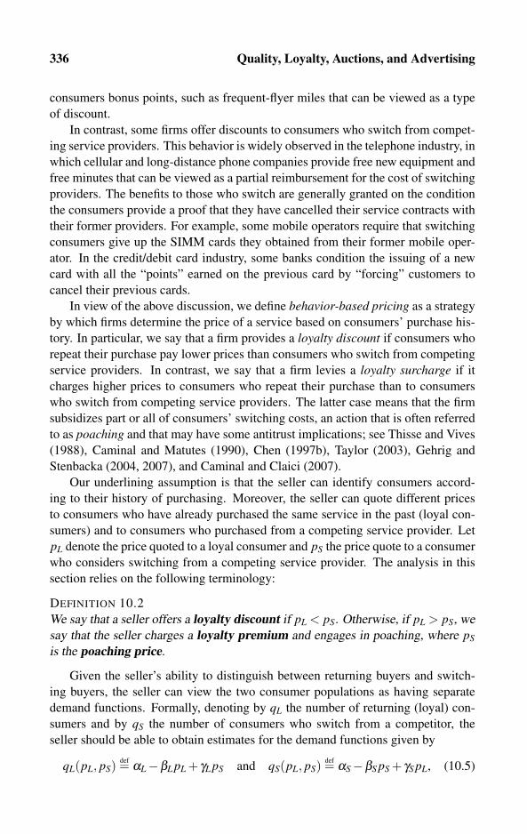
336 Quality, Loyalty, Auctions, and Advertising
consumers bonus points, such as frequent-flyer miles that can be viewed as a type
of discount.
In contrast, some firms offer discounts to consumers who switch from compet-
ing service providers. This behavior is widely observed in the telephone industry, in
which cellular and long-distance phone companies provide free new equipment and
free minutes that can be viewed as a partial reimbursement for the cost of switching
providers. The benefits to those who switch are generally granted on the condition
the consumers provide a proof that they have cancelled their service contracts with
their former providers. For example, some mobile operators require that switching
consumers give up the SIMM cards they obtained from their former mobile oper-
ator. In the credit/debit card industry, some banks condition the issuing of a new
card with all the “points” earned on the previous card by “forcing” customers to
cancel their previous cards.
In view of the above discussion, we define behavior-based pricing as a strategy
by which firms determine the price of a service based on consumers’ purchase his-
tory. In particular, we say that a firm provides a loyalty discount if consumers who
repeat their purchase pay lower prices than consumers who switch from competing
service providers. In contrast, we say that a firm levies a loyalty surcharge if it
charges higher prices to consumers who repeat their purchase than to consumers
who switch from competing service providers. The latter case means that the firm
subsidizes part or all of consumers’ switching costs, an action that is often referred
to as poaching and that may have some antitrust implications; see Thisse and Vives
(1988), Caminal and Matutes (1990), Chen (1997b), Taylor (2003), Gehrig and
Stenbacka (2004, 2007), and Caminal and Claici (2007).
Our underlining assumption is that the seller can identify consumers accord-
ing to their history of purchasing. Moreover, the seller can quote different prices
to consumers who have already purchased the same service in the past (loyal con-
sumers) and to consumers who purchased from a competing service provider. Let
pL denote the price quoted to a loyal consumer and pS the price quote to a consumer
who considers switching from a competing service provider. The analysis in this
section relies on the following terminology:
DEFINITION 10.2
We say that a seller offers a loyalty discount if pL < pS. Otherwise, if pL > pS, we
say that the seller charges a loyalty premium and engages in poaching, where pS
is the poaching price.
Given the seller’s ability to distinguish between returning buyers and switch-
ing buyers, the seller can view the two consumer populations as having separate
demand functions. Formally, denoting by qL the number of returning (loyal) con-
sumers and by qS the number of consumers who switch from a competitor, the
seller should be able to obtain estimates for the demand functions given by
qL(pL, pS)def= αL−βL pL + γL pS and qS(pL, pS)
def= αS−βS pS + γS pL, (10.5)

10.3 More on Pricing under Competition 337
where βL, γL, βS, and γS are the demand parameters to be estimated by the econome-
trician of the firm. The parameters βL and βS, often called “own-price” parameters,
measure the sensitivity of quantity demanded to changes in the price quoted for
the specific consumer group. The parameters γL and γS, often called “cross-price”
parameters, measure how an increase in the price quoted to switching consumers
affects the demand by loyal consumers, and how a rise in the price quoted to loyal
consumers affects the demand by switching consumers, respectively. The param-
eters γL and γS can be positive or negative, or zero when cross-demand effects do
not exist.
Before computing the profit-maximizing prices, the seller must verify that the
estimated parameters satisfy
βL > 0, βS > 0, and 4βLβS > (γL + γS)2. (10.6)
The first two inequalities ensure downward-sloping demand functions. The third
inequality implies that the demand by each consumer type is more sensitive to
changes in the price quoted to this group than the price quoted to the other consumer
group. Specifically, the demand by loyal consumers is affected more strongly by
the price offer made to loyal consumers than by the price offer made to switching
consumers. Similarly, the demand by consumers who switch from a competitor is
more sensitive to the price offer made directly to them than by the price offer made
to loyal consumers who do not switch. In other words, the third restriction in (10.6)
implies that the own-price effects are stronger than the cross-price effects. Also,
from a technical perspective as demonstrated below, the third restriction ensures
that the seller’s profit function is strictly concave with respect to pL and pS.
On the seller’s cost side, φ denotes the fixed cost, whereas μL and μS denote
the cost per unit of service sold to a loyal and switching consumer, respectively.
Clearly, this formulation is general in the sense that it permits the analysis of equal
unit costs (μL = μS) as a special case. However, one can imagine cases in which
μL < μS in which the seller may have to modify the product or the service offered
to switching consumers to attract them to abandon their loyalty to a competitor.
Another interpretation of μL < μS would be that it is more costly to register and
train a switching consumer to use the product or service compared with a loyal
consumer, who is already familiar with the seller’s brand. We proceed with two
numerical examples, followed by a general formulation.
An example of a loyalty discount
Consider a special case of the system of demand functions (10.5) given by
qL(pL, pS) = 120−2pL + pS and qS(pL, pS) = 120− pS + pL. (10.7)
This system of demand functions assumes that βL = 2 > 1 = βS, meaning that loyal
consumers are more price sensitive than switching consumers. This may reflect
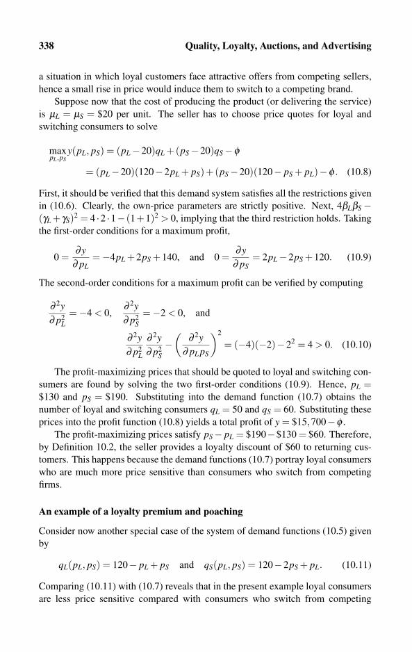
338 Quality, Loyalty, Auctions, and Advertising
a situation in which loyal customers face attractive offers from competing sellers,
hence a small rise in price would induce them to switch to a competing brand.
Suppose now that the cost of producing the product (or delivering the service)
is μL = μS = $20 per unit. The seller has to choose price quotes for loyal and
switching consumers to solve
maxpL,pS
y(pL, pS) = (pL−20)qL +(pS−20)qS−φ
= (pL−20)(120−2pL + pS)+(pS−20)(120− pS + pL)−φ . (10.8)
First, it should be verified that this demand system satisfies all the restrictions given
in (10.6). Clearly, the own-price parameters are strictly positive. Next, 4βLβS−(γL + γS)2 = 4 ·2 ·1− (1+1)2 > 0, implying that the third restriction holds. Taking
the first-order conditions for a maximum profit,
0 =∂y
∂ pL=−4pL +2pS +140, and 0 =
∂y∂ pS
= 2pL−2pS +120. (10.9)
The second-order conditions for a maximum profit can be verified by computing
∂ 2y∂ p2
L=−4 < 0,
∂ 2y∂ p2
S=−2 < 0, and
∂ 2y∂ p2
L
∂ 2y∂ p2
S−(
∂ 2y∂ pL pS
)2
= (−4)(−2)−22 = 4 > 0. (10.10)
The profit-maximizing prices that should be quoted to loyal and switching con-
sumers are found by solving the two first-order conditions (10.9). Hence, pL =$130 and pS = $190. Substituting into the demand function (10.7) obtains the
number of loyal and switching consumers qL = 50 and qS = 60. Substituting these
prices into the profit function (10.8) yields a total profit of y = $15,700−φ .
The profit-maximizing prices satisfy pS− pL = $190−$130 = $60. Therefore,
by Definition 10.2, the seller provides a loyalty discount of $60 to returning cus-
tomers. This happens because the demand functions (10.7) portray loyal consumers
who are much more price sensitive than consumers who switch from competing
firms.
An example of a loyalty premium and poaching
Consider now another special case of the system of demand functions (10.5) given
by
qL(pL, pS) = 120− pL + pS and qS(pL, pS) = 120−2pS + pL. (10.11)
Comparing (10.11) with (10.7) reveals that in the present example loyal consumers
are less price sensitive compared with consumers who switch from competing

10.3 More on Pricing under Competition 339
brands. This situation arises when loyal consumers have high costs of switching to
competing brands, for example, if the competing service is less consumer friendly
than the currently consumed brand.
The derivation of the profit-maximizing prices pL and pS is identical to the
previous case as it follows exactly the steps given by (10.8), (10.9), and (10.10).
For this reason, we state only the solution that is given by the prices pL = $190 and
pS = $130, demand levels qL = 60 and qS = 50, and total profit y = $15,700−φ .
In fact, one could have guessed this particular solution in view of the symmetry
between the demand systems (10.11) with (10.7).
Under the demand functions (10.11), the seller subsidizes the cost of consumers
switching from a competing brand by reducing the price for these consumers by
pS− pL = $60. Some literature refers to the lower pS as a poaching price. Another
interpretation that is also consistent with Definition 10.2 is that this seller charges
a loyalty premium to returning consumers as, according to (10.11), their demand is
less sensitive to price relative to the demand by consumers switching from compet-
ing brands.
General formulation
We now briefly repeat the previous derivations using a general notation that allows
for arbitrary values for the parameters of the demand functions (10.5). The seller
solves
maxpL,pS
y(pL, pS) = (pL−μL)qL +(pS−μS)qS−φ
= (pL−μL)(αL−βL pL + γL pS)+(pS−μS)(αS−βS pS + γS pL)−φ . (10.12)
At this stage, it should be verified that this demand system satisfies all the restric-
tions given by (10.6). Taking the first-order conditions for a maximum profit,
0 =∂y
∂ pL=−2pLβL + pS(γL + γS)+αL +βLμL− γSμS, (10.13)
0 =∂y
∂ pS= pL(γL + γS)−2pSβS +αS +βSμS− γLμL. (10.14)
The second-order conditions imply that the parameters of the model should satisfy
∂ 2y∂ p2
L=−2βL < 0,
∂ 2y∂ p2
S=−2βS < 0, and
∂ 2y∂ p2
L
∂ 2y∂ p2
S−(
∂ 2y∂ pL pS
)2
= (−2βL)(−2βS)− (γL + γS)2 > 0, (10.15)

340 Quality, Loyalty, Auctions, and Advertising
which explains why (10.6) must be assumed to be able to solve this maximization
problem.
Next, solving the two first-order conditions (10.13) yields
pL =2αLβS +(αS− γLμL)(γL + γS)+2βLβSμL +βSμS(γL− γS)
4βLβS− (γL + γS)2,
(10.16)
pS =2αSβL +(αL− γSμS)(γL + γS)+2βLβSμS +βLμL(γS− γL)
4βLβS− (γL + γS)2.
Finally, the quantity demanded by each consumer group, qL and qS, can be
found by substituting the equilibrium prices (10.16) into the demand functions
(10.5). The resulting profit is found by substituting the equilibrium prices (10.16)
into (10.12).
10.3.2 Price matching
Price matching, often referred to as “meeting (or even beating) the competition,”
is a statement and a commitment made by a seller to match or to beat price offers
made by competing sellers. Of course, such a commitment is generally limited to
a certain time period, such as one week. This section demonstrates that stores may
find such a commitment to be profit enhancing. It should be noted, however, that
in some cases economists may consider meeting or beating the competition to be a
violation of antitrust law as it may prevent sellers from being engaged in intensive
price competition; see Motta (2004, Ch. 4). Price matching and beating strategies
have been analyzed in a number of articles; to state a few, see Salop (1986), Belton
(1987), Png and Hirshleifer (1987), Doyle (1988), Logan and Lutter (1989), Corts
(1995, 1997), Hviid and Shaffer (1999), and Kaplan (2000).
Consider two adjacent stores labeled A and B that are located in the same shop-
ping mall and sell identical YNOS digital video players (DVD). Each store buys
directly from YNOS (the manufacturer) at a cost of μ = $50 per unit. Let φ ≥ 0
denote a store’s fixed cost of operation. Each day, 200 potential customers enter
this shopping mall with the intention of buying a YNOS DVD. Each consumer has
a 50% probability of patronizing store A first (and 50% of patronizing store B first).
Figure 10.3 demonstrates the well-known outcome of price competition leading to
unit-cost pricing. Figure 10.3 illustrates 200 consumers who are initially equally
split between the stores. With 50% probability, each store expects 100 consumers
to enter its store first before they proceed to the competing store to request a second
price offer for the same YNOS DVD.
Illustration I in Figure 10.3 reflects an initial situation in which both stores
quote a price of $80. Because this price exceeds the unit cost by $30, each store
makes a profit of yA(80,80) = yB(80,80) = 100(80−50)−φ = $3000−φ .
Because both stores are located in the same shopping mall, consumers can al-
most costlessly obtain a second price offer from the competing store. Illustration II

10.3 More on Pricing under Competition 341
pA = $80 pB = $80
100100
pA = $80 pB = $75
100100
pA = $50 pB = $50
100100=⇒ ·· ·=⇒ ···
yA = 0 yB = $5,000
A B A AB B
yA = yB = $3,000 yA = yB = 0
I. Unstable II. Undercutting III. Equilibrium
Figure 10.3: Price competition without price matching. Note: The fixed cost φ should be
subtracted from all profits.
shows the gain to store B from undercutting the price of store A by $5. Setting
pB = $75 implies that even consumers who initially go to store A and then get a
second offer from store B will not return to store A. Consumers who initially enter
store B and then compare their price offer with store A will go back to store B.
Hence by undercutting, store B captures the entire market and earns a profit of
yB(80,75) = 200(75−50)−φ = $5000−φ .
Illustration III in Figure 10.3 shows the resulting Nash-Bertrand equilibrium of
this price game, where undercutting leads to unit-cost pricing pA = pB = $50, and
hence to zero or negative profit yA(50,50) = yB(50,50) = 0−φ .
Suppose now that each store promises all consumers who enter to obtain a price
offer that it will match any price offered by the competing store. Figure 10.4 illus-
trates the consequences of such a commitment. Under the price-matching commit-
ment, store A (similarly store B) announces an initial price of pA = $80, which is far
above the unit cost of μ = $50. Store B has two options. It can undercut store A by
setting a lower price of pB = $75 as illustrated by the northeast arrow in Figure 10.4.
Consumers who first patronized store A will return to store A, which will match the
price of store B by p′A = $75. Now, with 200 consumers who are initially equally
split between the stores, each store ends up selling to 100 consumers. The resulting
expected profit levels are therefore yA = yB = 100(75−50)−φ = $2500−φ .
�
�
•
pB = $75
pB = $80
�
�
p′A = $75
pA = $80
•
•
Undercut
Maintain
Maintain
Match
B
A
A
yA = yB = $2500
yA = yB = $3000
pA = $80�•
A
Figure 10.4: Price competition with price matching. Note: The fixed cost φ should be
subtracted from all profits.

342 Quality, Loyalty, Auctions, and Advertising
In contrast, the southeast arrow in Figure 10.4 illustrates a second option avail-
able to store B, which is to maintain the same price as store A so that pB = pA = $80.
In this case, consumers cannot benefit from visiting more than one store; hence,
each store sells to 100 consumers who randomly enter each store. The resulting
expected profits are yA = yB = 100(80−50)−φ = $3000−φ . The key idea here is
that under the price-matching commitment by store A, store B cannot enhance itsprofit by undercutting the price of store A because store A will immediately match
its price. Thus, the price-matching commitment by store A creates an incentive for
store B to maintain a high price. For this reason, the “meeting the competition”
price strategy is often regarded as a facilitating practice because it relaxes price
competition to some degree.
The above model assumes that the two stores are located near each other, so
consumers can costlessly compare prices, and can costlessly return to the first store
they entered and demand that the store fulfil its commitment to match a lower price.
A natural question to ask at this point is, What happens if the stores are located at
different shopping malls, so consumers bear some time and transportation costs in
going back and forth between stores? However, such an environment has already
been analyzed in Section 3.4.1, which assumed that consumers bear some switching
costs in changing suppliers. Application of this model to price matching would
require that stores make their price cuts exceed consumers’ traveling cost in going
back to a store to ask that store to match the price of its rival. Consumers then will
have to evaluate the potential gain from traveling to a different store to obtain a
lower price, against their loss of value of time. The price level of the product would
clearly play a major role in this decision, as consumers are less likely to travel to
gain a price reduction of a few cents.
To overcome consumers’ transportation costs, stores can offer to beat the com-
petition instead of just matching a price, which would reward consumers who return
to a store by reducing the price strictly below that of a competing store. Clearly,
because price matching and price-beating announcements made by stores located
far apart from each other are also widely observed, we can conclude that the logic
of the model presented in this section also applies to citywide store competition.
Finally, price matching could become a risky business if the seller is unsure
of the cost borne by competitors. If competing sellers happen to have lower per-
unit costs, matching the price of rival stores may turn into a loss. In this respect,
sellers who are not sure whether they have a cost advantage or a disadvantage over
their rivals should make a meet-or-release commitment that enables the sellers to
compensate buyers with a full refund in the event they cannot profitably match the
price of a competing seller.
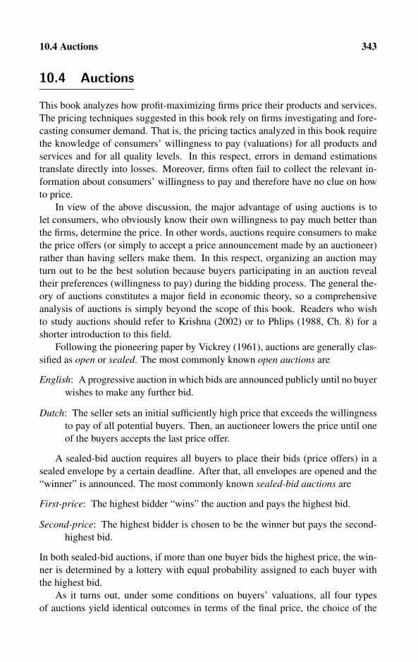
10.4 Auctions 343
10.4 Auctions
This book analyzes how profit-maximizing firms price their products and services.
The pricing techniques suggested in this book rely on firms investigating and fore-
casting consumer demand. That is, the pricing tactics analyzed in this book require
the knowledge of consumers’ willingness to pay (valuations) for all products and
services and for all quality levels. In this respect, errors in demand estimations
translate directly into losses. Moreover, firms often fail to collect the relevant in-
formation about consumers’ willingness to pay and therefore have no clue on how
to price.
In view of the above discussion, the major advantage of using auctions is to
let consumers, who obviously know their own willingness to pay much better than
the firms, determine the price. In other words, auctions require consumers to make
the price offers (or simply to accept a price announcement made by an auctioneer)
rather than having sellers make them. In this respect, organizing an auction may
turn out to be the best solution because buyers participating in an auction reveal
their preferences (willingness to pay) during the bidding process. The general the-
ory of auctions constitutes a major field in economic theory, so a comprehensive
analysis of auctions is simply beyond the scope of this book. Readers who wish
to study auctions should refer to Krishna (2002) or to Phlips (1988, Ch. 8) for a
shorter introduction to this field.
Following the pioneering paper by Vickrey (1961), auctions are generally clas-
sified as open or sealed. The most commonly known open auctions are
English: A progressive auction in which bids are announced publicly until no buyer
wishes to make any further bid.
Dutch: The seller sets an initial sufficiently high price that exceeds the willingness
to pay of all potential buyers. Then, an auctioneer lowers the price until one
of the buyers accepts the last price offer.
A sealed-bid auction requires all buyers to place their bids (price offers) in a
sealed envelope by a certain deadline. After that, all envelopes are opened and the
“winner” is announced. The most commonly known sealed-bid auctions are
First-price: The highest bidder “wins” the auction and pays the highest bid.
Second-price: The highest bidder is chosen to be the winner but pays the second-
highest bid.
In both sealed-bid auctions, if more than one buyer bids the highest price, the win-
ner is determined by a lottery with equal probability assigned to each buyer with
the highest bid.
As it turns out, under some conditions on buyers’ valuations, all four types
of auctions yield identical outcomes in terms of the final price, the choice of the

344 Quality, Loyalty, Auctions, and Advertising
winner, and the revenue collected by the seller. In particular, the open English auc-
tion and the second-price sealed bid auction yield identical outcomes in all respects
despite the fact that the English auction is open and requires the presence of all
bidders, whereas the other is sealed and does not require active participation on the
part of bidders as bidders can simply mail their sealed envelopes from a distance.
In addition to yielding identical outcomes, the open English auction and the
sealed-bid second-price auction share two additional common features. First, bid-
ders end up revealing their true willingness to pay during the auction process. Sec-
ond, bidders’ decisions are easy to establish because these decisions are not based
on any attempt on the part of bidders to predict the bids made by competing bidders.
Technically speaking, in these two auctions, bidders select their value-maximizing
bids based on their own valuations only. In contrast, in the open Dutch and the
sealed-bid first-price auctions, bidders must form some expectations on the bids
made by other participating bidders. For example, a bidder participating in the
sealed-bid first-price auction would benefit from knowing whether her bid is likely
to be above or below that of the competing bidders. If the buyer bids far above the
others, this buyer may benefit from lowering the bid. In contrast, if the buyer bids
slightly below the others, this buyer can win the auction by slightly increasing the
bid.
The above discussion implies that any analysis of the open Dutch and the
sealed-bid first-price auctions requires the imposition of some ad hoc assumptions
concerning the distribution of bidders’ valuations, and how each bidder perceives
this distribution when making the decision on how much to bid. For this reason,
Section 10.4.1 starts with the simple open English and sealed-bid second-price auc-
tions. Section 10.4.2 addresses the more complicated auctions that rely on various
assumptions concerning how bidders perceive the distribution of willingness to pay
of competing bidders.
Suppose there are M potential buyers who bid for a product or a service deliv-
ered by a single seller or a firm. Buyer �’s maximum willingness to pay (valuation)
is V�, where V� ≥ 0. Each buyer bids a price pb� , where 0 ≤ pb
� ≤ V�. If buyer �places the winning bid, the winner will pay pw. Note that in some auctions (such
as the sealed-bid second-price auction), the winner may end up paying a price that
is lower than the bid made by the winner. In any event, the payoff to the winner is
V�− pw. The payoff to a loser is normalized to equal 0.
10.4.1 Open English and sealed-bid second-price auctions
The open English and the sealed-bid second-price auctions are grouped together
not only because they always yield the same outcome, but because they are simple
to analyze. The simplicity arises because the participating bidders do not have to
form expectations or to forecast the valuations of competing bidders. Table 10.3
displays a sample of three auctions with five participating buyers.

10.4 Auctions 345
Auction # V1 V2 V3 V4 V5
1 $99 $100 $98 $80 $70
2 $100 $60 $100 $30 $65
3 $20 $20 $20 $100 $20
Table 10.3: Bidders’ valuations in three auctions.
Open English auction
Consider auction #1 in Table 10.3. In an English auction, the auctioneer announces
ascending prices 1,2, . . ., and so on. When the auctioneer announces p = $70, buyer
� = 5 opts out. Similarly, buyer � = 4 opts out at p = $80, buyer � = 3 opts out at
p = $98, and finally buyer � = 1 opts out at p = $99. Consequently, buyer � = 2
is announced to be the “winner” and pays pw = $99. The winner’s utility from
this auction is V2− pw = 100−99 = $1. Notice that under the English auction (as
well as in some other auctions), the seller can rarely capture the entire surplus from
buyers. To see this more clearly, consider auction #3 in Table 10.3. In this auction,
bidders 1, 2, 3, and 5 opt out when the auctioneer announces p = $20. The winner,
buyer � = 4 with a maximum willingness to pay of V4 = $100, ends up paying only
$20.
Under auction #2, the auctioneer raises the price until pw = $100 at which point
both remaining buyers opt out at the same time. The auctioneer than flips a coin and
determines, say, that buyer � = 3 is the winner, in which case the winning price is
set to pw = $100 and the winner obtains a utility of V3− pw = 100−100 = 0. Here,
the seller manages to extract the maximum surplus from bidders. Thus, sellers can
gain a lot when the two highest bidders have the same valuation.
Sealed-bid second-price auction
Suppose now that buyers are required to submit their bids to the seller in sealed
envelopes. When the deadline is reached, the seller opens all the envelopes and
announces the winner according to the highest bid. However, the winner is required
to pay only the price bid by the second-highest bidder.
The extremely attractive feature of the sealed-bid second-price auction is that
buyers have the incentives to bid their true valuation. Using the language of game
theory, the outcome from each buyer bidding his or her true valuation constitutes a
Nash equilibrium. Technically speaking, there may be some other Nash equilibria;
however, from a practical viewpoint, the lesson to be learned here is that it is never
a bad idea for a bidder to bid his or her true valuation no matter what bids are made
by other bidders. This happens because winners generally do not have to pay the
price according to their bid, but according to that of the second-highest bidder. To
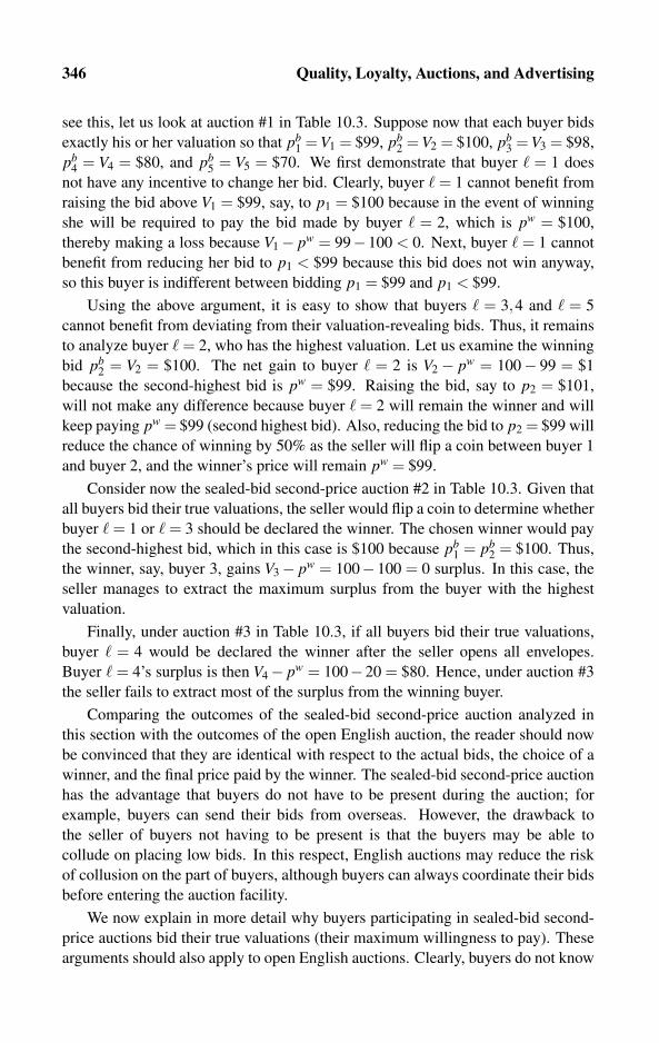
346 Quality, Loyalty, Auctions, and Advertising
see this, let us look at auction #1 in Table 10.3. Suppose now that each buyer bids
exactly his or her valuation so that pb1 = V1 = $99, pb
2 = V2 = $100, pb3 = V3 = $98,
pb4 = V4 = $80, and pb
5 = V5 = $70. We first demonstrate that buyer � = 1 does
not have any incentive to change her bid. Clearly, buyer � = 1 cannot benefit from
raising the bid above V1 = $99, say, to p1 = $100 because in the event of winning
she will be required to pay the bid made by buyer � = 2, which is pw = $100,
thereby making a loss because V1− pw = 99−100 < 0. Next, buyer � = 1 cannot
benefit from reducing her bid to p1 < $99 because this bid does not win anyway,
so this buyer is indifferent between bidding p1 = $99 and p1 < $99.
Using the above argument, it is easy to show that buyers � = 3,4 and � = 5
cannot benefit from deviating from their valuation-revealing bids. Thus, it remains
to analyze buyer � = 2, who has the highest valuation. Let us examine the winning
bid pb2 = V2 = $100. The net gain to buyer � = 2 is V2 − pw = 100− 99 = $1
because the second-highest bid is pw = $99. Raising the bid, say to p2 = $101,
will not make any difference because buyer � = 2 will remain the winner and will
keep paying pw = $99 (second highest bid). Also, reducing the bid to p2 = $99 will
reduce the chance of winning by 50% as the seller will flip a coin between buyer 1
and buyer 2, and the winner’s price will remain pw = $99.
Consider now the sealed-bid second-price auction #2 in Table 10.3. Given that
all buyers bid their true valuations, the seller would flip a coin to determine whether
buyer � = 1 or � = 3 should be declared the winner. The chosen winner would pay
the second-highest bid, which in this case is $100 because pb1 = pb
2 = $100. Thus,
the winner, say, buyer 3, gains V3− pw = 100− 100 = 0 surplus. In this case, the
seller manages to extract the maximum surplus from the buyer with the highest
valuation.
Finally, under auction #3 in Table 10.3, if all buyers bid their true valuations,
buyer � = 4 would be declared the winner after the seller opens all envelopes.
Buyer � = 4’s surplus is then V4− pw = 100−20 = $80. Hence, under auction #3
the seller fails to extract most of the surplus from the winning buyer.
Comparing the outcomes of the sealed-bid second-price auction analyzed in
this section with the outcomes of the open English auction, the reader should now
be convinced that they are identical with respect to the actual bids, the choice of a
winner, and the final price paid by the winner. The sealed-bid second-price auction
has the advantage that buyers do not have to be present during the auction; for
example, buyers can send their bids from overseas. However, the drawback to
the seller of buyers not having to be present is that the buyers may be able to
collude on placing low bids. In this respect, English auctions may reduce the risk
of collusion on the part of buyers, although buyers can always coordinate their bids
before entering the auction facility.
We now explain in more detail why buyers participating in sealed-bid second-
price auctions bid their true valuations (their maximum willingness to pay). These
arguments should also apply to open English auctions. Clearly, buyers do not know

10.4 Auctions 347
whether they have the highest valuation (and thus will win the auction) or not. The
following list of arguments proves that bidders cannot benefit from deviating from
bidding their true valuations.
(1) The bidder with the highest valuation wins the auction given that all other buy-
ers bid their true (lower) valuations. Hence, increasing the bid beyond the true
valuation will not make any difference for the winning buyer.
(2) The bidder with the highest valuation cannot benefit from reducing the bid
below the true valuation because the winner pays only the second-highest price
bid (and not the highest bid). Hence, reducing the bid will not reduce the price
actually paid by the winner but may result in not winning the auction if the
reduced bid falls below the valuation of some other bidder.
(3) Bidders with lower valuations cannot benefit from increasing their bids above
their true valuations, as in the event they win the auction they will be forced to
pay a price above their maximum willingness to pay and end up with negative
surplus.
(4) Bidders with lower valuations cannot benefit from reducing their bids below
their true valuations because they do not win the auction in any event.
10.4.2 Open Dutch and sealed-bid first-price auctions
In an open Dutch auction, the auctioneer starts with a very high price (above all
possible valuations) and gradually reduces the price until a buyer agrees to pay.
Under independent valuations, it turns out that this auction generates the same out-
come as the sealed-bid first-price auction, in which all buyers place their bids in
sealed envelopes and the highest bidder wins and pays the highest bid (as opposed
to a sealed-bid second-price auction, which we have already analyzed). Given this
equivalence, the analysis below focuses on sealed-bid first-price auctions; however,
the reader should bear in mind that the bidding function (10.18) derived below ap-
plies to the open Dutch auction as well.
The analytical difficulty with these two auctions is that buyers must form ex-
pectations concerning the bids made by all other buyers. Different expectations will
result in different bids by all participants. The key assumption here is that buyers’
valuations are independent in the sense that each buyer is assumed to “draw” his
or her valuations from a distribution and that each draw is statistically independent
of draws made by rival buyers. In other words, buyers do not share any common
value. Clearly, this assumption is less appealing for financial products, for which
actions taken by some buyers (such as buyers who invest in stocks) signal to other
buyers the value of the goods.
Suppose there are M potential buyers who bid for a single product or service
offered by the seller. Each buyer knows his or her own valuation but does not know

348 Quality, Loyalty, Auctions, and Advertising
the valuations of competing buyers, except that all valuations are drawn uniformly
from the interval [V L,V H ] with equal probability, where V H > V L ≥ 0. Figure 10.5
illustrates the distribution of buyers’ valuations and the corresponding probability
distribution.
� V�0 V L V H
1
0
�
V
�
Pr{V L ≤V ≤ V}
Figure 10.5: Independently distributed buyers’ valuations.
The horizontal axis of Figure 10.5 measures buyers’ possible valuations, which
lie on the interval V L ≤ V� ≤ V H . Each buyer knows his or her own valuation
for certain, but perceives other buyers’ valuations as randomly distributed on this
interval with equal probability. The vertical axis measures the probability that a
competing buyer �’s valuation is in the range of V L ≤V� ≤ V . Formally, under the
assumed uniform distribution, this probability is given by
Pr{V L ≤V ≤ V}=V −V L
V H −V L . (10.17)
For example, according to (10.17), the probability that a buyer’s valuation is V =V H or lower is Pr{V L ≤ V ≤ V H} = (V H −V L)/(V H −V L) = 1. Similarly, the
probability that a buyer’s valuation is V = V L or lower is Pr{V ≤ V L} = (V L−V L)/(V H−V L) = 0, simply because there are no buyers with valuations below V L.
The time line for this sealed-bid first-price auction is as follows: First, each
buyer � learns his or her own valuation V�. Then, each buyer places a bid in a
sealed envelope knowing only that there are other M−1 competing buyers whose
valuations are randomly drawn from the distribution (10.17), who also place their
bids in sealed envelopes. Finally, the seller opens all envelopes and awards the
product/service to the highest bidder, who has to pay the highest price.
We first postulate and then prove the equilibrium bids for the above-described
auction. In this equilibrium, each bidder � with valuation V� bids
p� =(M−1)V� +V L
M, for each buyer � = 1,2, . . . ,M. (10.18)
In the language of game theory, the M equations in (10.18) constitute a Nash equi-
librium. In a Nash equilibrium, no bidder � could benefit from unilaterally deviating
from the bid (10.18), given that all other bidders stick to their bids as described by

10.4 Auctions 349
�V H
V L
� V�
V L V H
p�
V H+V L
2
����
����� p�(V�) for M = 2
p�(V�) for M = 3
���������
p�(V�) as M→ ∞
Figure 10.6: Equilibrium bids in sealed-bid first-price auctions as functions of buyers’ val-
uations.
(10.18). The bid functions defined by (10.18) are drawn in Figure 10.6. As in Fig-
ure 10.5, the horizontal axis of Figure 10.6 measures buyers’ possible valuations on
the interval V L ≤V� ≤V H . The vertical axis measures the bid made by each buyer
as a function of the buyer’s valuation V�.
It follows directly from (10.18) or Figure 10.5 that the equilibrium bids have
the following properties:
(a) Bids increase monotonically with valuations; that is, a buyer with a higher
valuation bids a price higher than that of buyers with low valuations. Formally,
p� ≥ pk whenever V� ≥Vk, for all buyers �,k = 1,2, . . . ,M.
(b) A buyer with the lowest valuation V L always bids p = V L. All other buyers bid
below their valuations so that p� < V� if V L < V �.
(c) All bids (except perhaps the lowest bid) increase when the number of buyers
increases. Formally, for every valuation V�, p�(V�) increases with M. In the
limit, when the number of buyers gets to be very large, all buyers bid their true
valuations. Formally, p�(V�)→V� as M→ ∞.
The reader may wonder why a buyer with the lowest valuation does not bid less than
his or her valuation V L. The reason is that this buyer actually never wins an auction
because no other buyer bids below V L, so there is no benefit from lowering the bid.
Next, when the number of buyers increases, each buyer has a lower probability of
winning, causing buyers to increase their bids.
We now prove that the M bids given by (10.18) indeed constitute a Nash equi-
librium. With no loss of generality, let us concentrate on the actions available to
buyer � = 1, who sets the bid p1. The probability that buyer � = 1 wins the auction
is
Pr{p1 > max{p2, p3, . . . , pM}}=(
p1− pL
pH − pL
)M−1
, (10.19)
350 Quality, Loyalty, Auctions, and Advertising
where pL and pH are the bids made by buyers who “draw” the extreme valuations
V L and V H , respectively, defined by
pL def= V L and pH def=(M−1)V H +V L
M. (10.20)
Buyer � = 1 seeks to maximize expected surplus, which is the difference between
her valuation and her bid (where the bid is also the price to be paid under a first-
price auction), multiplied by the probability that she is the winner. Formally, buyer
� = 1 chooses p1 to solve
maxp1
U1(p1) = maxp1
(V1− p1)(
p1− pL
pH − pL
)M−1
, (10.21)
where pL and pH are defined by (10.20). The expected surplus of buyer � = 1 is
strictly concave with respect to p1. The first-order condition for a maximum surplus
is therefore
0 =dU1(p1)
dp1=
M[M(V1− p1)−V1 + pL]p1− pL
(p1− pL
pH − pL
)M−1
. (10.22)
Substituting pL and pH from (10.20) into (10.22) and solving for p1 yields p1 =[(M− 1)V1 +V L]/M, which is exactly the same as the general solution given by
(10.18). This concludes the proof that the bids (10.18) indeed constitute a Nash
equilibrium.
10.4.3 Revenue equivalence under independent valuations
The objective of the seller is to maximize expected revenue from the sale of prod-
ucts and services via the use of auctions. This means that the seller would choose
the auction method that maximizes the expected price to be paid by the winner of
the auction. Therefore, a natural question to ask at this point is whether and how
the four auctions analyzed in this section differ with respect to the expected rev-
enue earned by the seller. As it turns out, if buyers’ valuations are independent
and are drawn from the same distribution (like the ones with the uniform distribu-
tion depicted in Figure 10.5), all four auctions generate exactly the same expected
revenue.
In what follows, we demonstrate how the sealed-bid second-price auction an-
alyzed in Section 10.4.1 and the sealed-bid first-price auction analyzed in Sec-
tion 10.4.2 yield identical expected revenue to the seller. In fact, this demonstration
is sufficient for showing that all four auctions are equivalent with respect to the
expected revenue they generate. To simplify the exposition, the following compu-
tations assume that V L = 0, which means that all buyers’ valuations are uniformly
distributed on the interval [0,V H ].
10.4 Auctions 351
Expected revenue generated by the sealed-bid second-price auction
Section 10.4.1 has shown that under the sealed-bid second-price auction all buyers
bid their true valuations. Therefore, because the winner ends up paying the second-
highest bid, expected revenue to the seller equals expected value of the second-
highest valuation.
The probability that all the M valuations are equal to or below V is (V/V H)M.
Next, the probability that a specific valuation is realized to be exactly the second-
highest is (1−V/V H)(V/V H)M−1, which is the product of the probability of having
one valuation higher than V and the probability that all remaining M−1 valuations
are below it. Altogether, the probability that the second-highest valuation does not
exceed V is the sum
(V
V H
)M
+M(
1− VV H
)(V
V H
)M−1
. (10.23)
The first term is the probability that all M buyers bid no higher than V . The second
term is the probability that one and only one buyer bids higher than the remaining
M− 1 buyers. The second term is multiplied by M because there are M buyers
who may turn out to have the second-highest valuation. Differentiating (10.23)
with respect to V yields the density associated with the distribution of the second-
highest valuation. Hence,
M(M−1)V M−2(V H −V )(V H)M . (10.24)
Therefore, the expected second-highest valuation, which also equals the expected
revenue to the seller, is computed by
Ex =V H∫0
M(M−1)V M−2(V H −V )(V H)M dV =
M−1
M +1V H . (10.25)
Thus, the seller’s expected revenue increases with the number of buyers partici-
pating in this auction. In the limit, when the number of participants becomes very
large, the expected revenue to the seller approaches the highest valuation. Formally,
Ex→ V H as M→ ∞. This happens because an increase in the number of partic-
ipants increases the probability that the buyer with the second-highest valuation
“draws” a higher valuation. In the limit, the second-highest valuation will be close
to V H .
Expected revenue generated by the sealed-bid first-price auction
The probability that the highest valuation among M buyers does not exceed Vis (V/V H)M. The density function associated with this probability is given by
352 Quality, Loyalty, Auctions, and Advertising
d(V/V H)M/dV = MV M−1(V H)−M, for 0 ≤ V ≤ V H . Using the bids of the first-
price auction given by (10.18), the expected highest bid, which also equals the
expected revenue to the seller, is computed by
Ex =V H∫0
[MV M−1
(V H)M
][(M−1)V
M
]dV =
M−1
M +1V H . (10.26)
The first term under the integral sign is the valuations’ density function. The second
term is the bid made by each buyer in a sealed-bid first-price auction.
Comparing (10.25) with (10.26) reveals that the expected seller’s revenue un-
der the first- and second-price sealed-bid auctions are the same. This means that
the open English ascending and Dutch descending price auctions also generate the
same expected seller’s revenue as in (10.25) and (10.26). In fact, all four auctions
are also “socially optimal” in the sense that the winner is always the buyer with the
highest valuation. It should be stressed that these equivalence results may fail to
hold when buyers’ valuations are not independent. For example, if buyers tend to
revise their valuations during an open English auction after the auctioneer raises the
price and most buyers agree to pay the higher price, then buyers may share a com-
mon value for the auctioned good, which is revealed during the auction process. In
this case, the above-mentioned equivalence results may not hold.
10.5 Advertising Expenditure
Pricing techniques often involve large investments in advertising. Advertising is
generally defined as a form of providing information about prices, quality, and the
location of goods and services. In practice, advertising often lacks some of these
features, and instead attempts to convey an image of the type of personalities associ-
ated with the advertised good. The economics literature distinguishes between two
types of advertising: persuasive advertising and informative advertising. Persua-
sive advertising intends to enhance consumer tastes for a certain product, whereas
informative advertising carries basic product information such as characteristics,
prices, and where to buy it.
Earlier modern authors, such as Kaldor (1950), held the idea that advertising
is “manipulative” and reduces competition and therefore reduces welfare for two
reasons: First, advertising persuades consumers to believe wrongly that identical
products are different because the decision of which brand to purchase depends on
consumers’ perception of the brand rather than on the actual physical characteris-
tics of the product. Therefore, prices of heavily advertised products may rise far
beyond their cost of production. Second, advertising serves as an entry-deterring
mechanism because any newly entering firm must extensively advertise to surpass
the reputation of the existing firms. Thus, existing firms use advertising as an entry-
10.5 Advertising Expenditure 353
deterrence strategy and can maintain their dominance while keeping above-normal
profit levels.
More-recent authors, such as Telser (1964), Nelson (1970, 1974), and Demsetz
(1979), proposed that advertising serves as a tool for transmitting information from
producers to consumers about different brands, thereby reducing consumers’ cost
of obtaining information about where to purchase their most preferred brand.
Nelson (1970) distinguishes between two types of goods: search goods and ex-perience goods. Consumers can identify the quality and other characteristics of the
product before the actual purchase of search goods. Examples include tomatoes or
shirts. Consumers cannot learn the quality and other characteristics of experience
goods before the actual purchase. Examples include new models of cars and many
electrical appliances with unknown durability and failure rates. Note that this dis-
tinction is not really clear-cut, because we cannot fully judge the quality of a tomato
until we eat it, and we cannot fully judge the quality of a shirt until after the first
wash!
10.5.1 Demand functions and advertising
To find out whether advertising enhances the demand for a seller’s products and
services, the econometrician has to estimate a demand that is a function of both
price and advertising expenditure. Clearly, if advertising has only a little effect on
the quantity demanded, the firm should not invest in advertising. In contrast, if the
demand is greatly enhanced by advertising, the firm may want to take into account
a possible trade-off between price reduction and advertising expenditure as both
contribute to demand increases.
As it turns out, an extended version of the constant-elasticity demand function
analyzed in Section 2.4 is very handy for determining the profit-maximizing ex-
penditure on advertising. Let a denote the firm’s expenditure on advertising. The
variables q and p denote the quantity demanded and the price set by the firm, re-
spectively. It is assumed that the quantity demanded is enhanced with an increase
in advertising expenditure, and declines with price. Formally, a constant-elasticity
demand as a function of price and advertising expenditure is defined by
q(a, p) def= α aea p−ep , where 0 < ea < 1 and ep > 0 (10.27)
are the advertising elasticity and the price elasticity, respectively. Formally, in view
of the elasticity analysis of Section 2.4.3, the price elasticity is defined and com-
puted by
epdef=
∂q(a, p)∂ p
pq
=−α aea ep p−ep−1 pα aea p−ep
=−ep. (10.28)
Similarly, the advertising elasticity is defined and computed by
eadef=
∂q(a, p)∂a
aq
= α p−ep ea aea−1 aα aea p−ep
= ea. (10.29)

354 Quality, Loyalty, Auctions, and Advertising
Before the firm can make a decision on how much to spend on advertising, it
must estimate the parameters α , ea, and ep of the demand function (10.27). As
demonstrated in Section 2.4.2, perhaps the simplest way would be to form a linear
regression by taking the natural logarithm of (10.27), yielding
lnq︸ ︷︷ ︸ln quantity
= lnα︸ ︷︷ ︸constant
+ ea︸︷︷︸elasticity
lna︸ ︷︷ ︸ln advertising
− ep︸︷︷︸elasticity
ln p︸ ︷︷ ︸ln price
. (10.30)
Using past data on prices and advertising expenditure, the econometrician of the
firm should be able to estimate the parameter α and the two elasticities ea and
ep. For the following analysis to be valid, it must be verified that the estimated
elasticities ea and ep satisfy the restrictions stated in (10.27).
10.5.2 Profit-maximizing advertising expenditure
The constant-elasticity demand function (10.27) turns out to be very useful for com-
puting the profit-maximizing spending on advertising. For this demand function,
Dorfman and Steiner (1954) established that a monopoly’s profit-maximizing ad-
vertising and price levels should be set so that the ratio of advertising expenditureto revenue equals the (absolute value of the) ratio of the advertising elasticity toprice elasticity. Formally,
apq
=ea
−ep. (10.31)
The left side of (10.31) is the ratio of how much the firm should invest in advertis-
ing, a, to sales revenue, x = pq, made by this firm. The right side is the ratio of the
two estimated demand elasticities. Thus, this firm should increase its advertising-
to-sales ratio as the demand it faces becomes more elastic with respect to adver-
tising (ea gets closer to 1), or less elastic with respect to price (ep gets closer to
zero).
We conclude this analysis with a numerical example that demonstrates the use-
fulness of the formula given by (10.31). Suppose that the estimated advertising
elasticity is ea = 0.01, which means that a 1% increase in advertising expenditure
would result in a 0.01% increase in quantity demanded. Also suppose that the
price elasticity was estimated to be −1.2, which means that a 1% drop in price
would result in a 1.2% increase in quantity demanded. We now compute the profit-
maximizing expenditure on advertising, assuming that sales revenue is estimated to
be around $120,000. Using the formula (10.31), the above data imply that
a$120,000
=0.01
−(−1.2)=⇒ a = $1000. (10.32)

10.6 Exercises 355
10.6 Exercises
1. Congratulations! You have been appointed chief engineer of GIBBERISH, a lead-
ing manufacturer of inkjet printers (printers that fire extremely small droplets of
ink on paper). Your team of engineers has informed you that the company is
able to produce printers of three quality levels: quality F , which is a fast 20
page–per-minute (PPM) printer; quality M, which is a medium-speed 15 PPM
printer; and quality S, which is a slow model capable of only 8 PPM.
Your colleagues at the marketing department have been conducting market sur-
veys to approximate potential buyers’ willingness to pay for the different qual-
ities, which are summarized in Table 10.4. Table 10.4 also displays the unit
production cost of each printer according to quality. Solve the following prob-
lems assuming that there are no fixed costs, φ = 0.
i (Quality) � = 1 � = 2 μi (Unit Cost)
F (Fast) V F1 = $70 V F
2 = $50 μF = $50
M (Medium) V M1 = $65 V M
2 = $40 μM = $30
S (Slow) V S1 = $40 V S
2 = $30 μS = $10
N� (# consumers) N1 = 50 N2 = 40
Table 10.4: Data for Exercise 1.
(a) Compute the profit GIBBERISH earns when it sells quality F only, quality Monly, and quality S only.
(b) Conclude which quality GIBBERISH should introduce into the market, as-
suming that only one quality can be sold in this market.
(c) Using the analysis of Section 10.1.4, determine whether GIBBERISH can
enhance its profit by introducing more than one model into the market. If
your answer is positive, indicate which printer models should be introduced
and their profit-maximizing prices. Prove that these prices indeed segment
the market in the sense that each model introduced into the market will be
demanded by at least one type of consumers.
2. Your company can produce a 20 PPM laser printer at a cost of $50 per unit. In
addition, your firm can replace a memory chip on each printer for an additional
cost of $10 per unit, which would slow the printer down to 10 PPM (thus raising
the unit cost of the damaged printer to $60 per unit). Table 10.5 displays poten-
tial consumers’ maximum willingness to pay for the two printer configurations.
Solve the following problems using the analysis of Section 10.2, assuming that
there are no fixed costs, φ = 0.
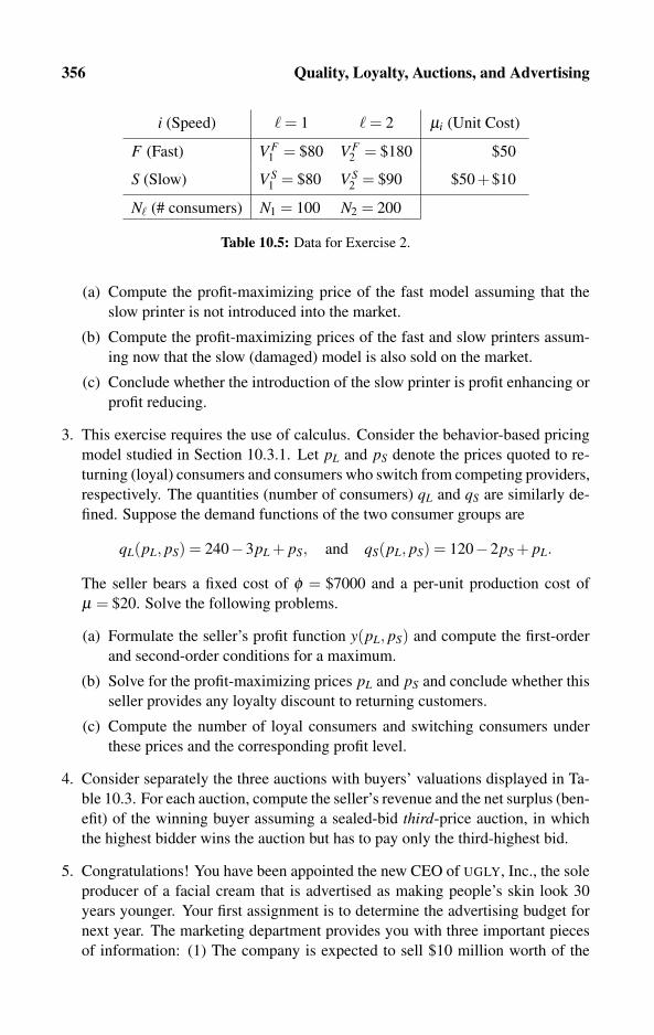
356 Quality, Loyalty, Auctions, and Advertising
i (Speed) � = 1 � = 2 μi (Unit Cost)
F (Fast) V F1 = $80 V F
2 = $180 $50
S (Slow) V S1 = $80 V S
2 = $90 $50+$10
N� (# consumers) N1 = 100 N2 = 200
Table 10.5: Data for Exercise 2.
(a) Compute the profit-maximizing price of the fast model assuming that the
slow printer is not introduced into the market.
(b) Compute the profit-maximizing prices of the fast and slow printers assum-
ing now that the slow (damaged) model is also sold on the market.
(c) Conclude whether the introduction of the slow printer is profit enhancing or
profit reducing.
3. This exercise requires the use of calculus. Consider the behavior-based pricing
model studied in Section 10.3.1. Let pL and pS denote the prices quoted to re-
turning (loyal) consumers and consumers who switch from competing providers,
respectively. The quantities (number of consumers) qL and qS are similarly de-
fined. Suppose the demand functions of the two consumer groups are
qL(pL, pS) = 240−3pL + pS, and qS(pL, pS) = 120−2pS + pL.
The seller bears a fixed cost of φ = $7000 and a per-unit production cost of
μ = $20. Solve the following problems.
(a) Formulate the seller’s profit function y(pL, pS) and compute the first-order
and second-order conditions for a maximum.
(b) Solve for the profit-maximizing prices pL and pS and conclude whether this
seller provides any loyalty discount to returning customers.
(c) Compute the number of loyal consumers and switching consumers under
these prices and the corresponding profit level.
4. Consider separately the three auctions with buyers’ valuations displayed in Ta-
ble 10.3. For each auction, compute the seller’s revenue and the net surplus (ben-
efit) of the winning buyer assuming a sealed-bid third-price auction, in which
the highest bidder wins the auction but has to pay only the third-highest bid.
5. Congratulations! You have been appointed the new CEO of UGLY, Inc., the sole
producer of a facial cream that is advertised as making people’s skin look 30
years younger. Your first assignment is to determine the advertising budget for
next year. The marketing department provides you with three important pieces
of information: (1) The company is expected to sell $10 million worth of the
10.6 Exercises 357
product. (2) It is estimated that a 1% increase in the advertising budget would
increase the quantity sold by 0.05%. (3) It is also estimated that a 1% increase
in the product’s price would reduce quantity sold by 0.2%.
(a) How much money would you allocate for advertising next year?
(b) Now, suppose the marketing department has revised its estimation regarding
the demand price elasticity to a 1% increase in price, resulting in a reduc-
tion in quantity sold by 0.5%. How much money would you allocate to
advertising after getting the revised estimate?
(c) Conclude how a change in the demand price elasticity affects advertising
expenditure.

Chapter 11
Tariff-choice Biases and Warranties
11.1 Flat-rate Biases 36011.2 Choice in Context and Extremeness Aversion 36211.3 Other Consumer Choice Biases 366
11.3.1 Odd pricing and the 99/c fixation
11.3.2 Price–quality perceptions
11.3.3 Micropayments and currency denomination
11.4 Warranties 36911.4.1 Product replacement warranties
11.4.2 Money-back guarantee
11.5 Exercises 375
The pricing techniques described throughout this book are based on the presump-
tion that buyers always optimize their selections among the different payment plans
and quality classes that are offered by one or more sellers. By optimizing, we mean
that buyers operate according to well-defined objectives, such as expenditure min-
imization, maximization of value versus price, and minimization of expected price
in case of uncertainty. Sadly enough for academic economists, consumers do not
always behave this way. More precisely, consumers often end up selecting a pay-
ment plan, a brand, or a quality level that seems to violate consumers’ objective
functions as commonly assumed by economists.
The development of profitable marketing and pricing strategies requires an un-
derstanding of the manner in which consumers choose among alternatives. This
chapter is devoted almost entirely to consumers who seem to be optimizing in
ways different from those we have assumed so far in this book. The basic idea
is that firms should often take into account what sometimes looks like an irrational
behavior on the part of consumers and set their price menus accordingly. In fact,
in many instances firms can actually take advantage of certain “odd” consumer be-
haviors and extract an even higher surplus from these consumers compared with
the surplus that can be extracted from consumers who behave according to the way
economists want them to behave.
360 Tariff-choice Biases and Warranties
The examination of consumer behavior combines aspects from psychology and
economics. That is, the psychology of decision making turns out to be helpful
in explaining the observed anomalies on the part of consumers. Along this line,
some researchers even argue that consumers often lack the ability to make optimal
choices. This is especially true when service providers offer consumers complex
packages under which consumers find it difficult to estimate their actual costs. Such
complex packages are widely observed in the telephone industry. Consumers’ in-
ability to consider all possibilities is known as bounded rationality, a term attributed
to Simon (1955); see also Kahneman (2003) for recent applications.
The psychological, social, and economic motivations for what appear to be
irrational choices on the part of consumers have recently earned a field name in
economics called behavioral economics. Clearly, this name choice is rather poor
because all the major fields that fall under the categories of psychology, sociology,
and economics are concerned with modeling human behavior. However, this name
serves its purpose as economists nowadays refer to behavioral economics as the
study of consumer choice anomalies. A wide variety of these anomalies have been
studied over the years; see Thaler (1991, 1992), and in the context of behavioral
economics, see Mullainathan and Thaler (2000) and Camerer, Loewenstein, and
Rabin (2003). In this chapter, we obviously focus only on some anomalies related
to pricing. For more comprehensive discussions and research surveys on consumer
perceptions with respect to prices, the reader is referred to Wilkie (1990), Monroe
(2002), and Winer (2005).
This chapter ends with the analysis of warranties. Warranties serve two pur-
poses: The first, which is not necessarily related to behavioral economics, serves
as insurance to consumers against defects in the products or services they buy. The
second is a psychological comfort for which consumers are willing to pay extra.
11.1 Flat-rate Biases
It is widely observed that consumers subscribing to services prefer flat-rate pay-
ment plans over paying separately for each unit of consumption, despite the fact
that very often flat-rate plans turn out to be more expensive than the sum of all pay-
per-use fees and prices under the measured plans. The following list summarizes
some of the explanations given in the literature for this anomaly.
Insurance: Risk-averse consumers use the flat-rate option to obtain full insurance
against realizations of high demand. According to this view, risk-averse con-
sumers may hedge against an abnormally high bill by paying a flat rate. Thus,
pay per use constitutes the riskiest billing plan.
Aversion to being metered: Also known as the taxi meter effect, consumers simply
do not like to be monitored with respect to their consumption level.

11.1 Flat-rate Biases 361
High expectations: For some services, consumers consistently overestimate their
actual use. For example, health-oriented consumers tend to make New Year’s
resolutions to visit their health clubs more often than they actually do.
Time-inconsistent preferences: Consumers are fully aware of their initially high
consumption expectations and the fact that their willingness to pay will di-
minish over time.
Convenience and confusion: Consumers are often confused when offered a wide
variety of payment plans in the form of packages. The flat-rate payment plan
is perceived as the simplest plan and is therefore the most convenient. In
addition, the flat-rate plan reduces transaction costs.
Option value: People are simply willing to pay extra for the option of using the
service at zero marginal usage price.
The anomaly concerning consumers’ choice of the flat-rate plan instead of the
pay-per-use plan despite the common observation that the latter turns out to be
cheaper has been described and analyzed in a variety of papers, including Train,
McFadden, and Ben-Akiva (1987); Train, Ben-Akiva, and Atherton (1989); Mitchell
and Vogelsang (1991, pp. 176–177); Clay, Sibley, and Srinagesh (1992); Kridel,
Lehman, and Weisman (1993); Danielsen, Kamerschen, and Nicolaou (1993); and
Miravete (2003). Nunes (2000) reports on surveys showing that people are gener-
ally willing to pay a large premium for unlimited access to online shopping, even
when neither their current nor their expected usage can justify it. The same paper
also presents a different study of health club users in Chicago demonstrating the
bias toward a flat-rate membership plan relative to paying for each visit separately.
DellaVigna and Malmendier (2006) provide an empirical analysis of the time in-
consistency associated with choices in health club membership plans. Lambrecht
and Skiera (2006) conduct empirical analyses on the various causes of the flat-rate
bias.
Table 11.1 displays some real-life data for three service industries that offer flat-
rate subscription and pay-per-use payment plans. The second column of Table 11.1
displays the flat-rate subscription fee f . The third column displays the per-unit
price p if a subscription is not made, and the fourth displays the actual observed
quantity of the service q used. The fifth column displays the hypothetical total
expenditure p ·q that would be borne had the consumer chosen not to subscribe to
the flat-rate plan. The sixth column displays the price per use f /q actually paid,
which equals the flat-rate subscription fee divided by the quantity used.
For the health club market, the three variables f , p, and q are averages for
flat-rate subscribers reported by Nunes (2000) and DellaVigna and Malmendier
(2006). Nunes (2000) reports on 79 regular club users who averaged q = 38 visits
per year and paid an annual membership fee of f = $610. Therefore, these users
paid an effective price of f /q = 610/38 ≈ $16.05 per visit despite the fact that a

362 Tariff-choice Biases and Warranties
Market f p q p ·q f /q
Health club (Y): $610.00 $10.00 38.00 $380.00 $16.05
Health club (M): $70.00 $10.00 4.80 $48.00 $14.58
Phone (low q): $19.85 $0.11 70 $7.70 $0.28
Phone (high q): $19.85 $0.11 101 $11.11 $0.20
Subscription (M): $19.95 $6.95 2.42 $16.85 $8.23
Table 11.1: Data on the use of flat rates for three service industries. Note: Y stands for
yearly membership, M for monthly membership.
one-time guest fee was $10 (an overpayment of 60%). DellaVigna and Malmendier
examine more than 7000 members of three New England health clubs. Their data
set contains information on the contractual choices and day-to-day attendance of
users from 1997 to the early 2000s. As these authors point out, with a monthly
average of q = 4.8 visits, consumers who subscribed to the monthly flat rate plan
ended up paying a price of f /q = $70/4.8≈ $14.6 per visit, despite the fact that the
pay-per-use plan was obtainable for $10 per visit. That is, consumers “overpaid”
46% more than they could have paid had they chosen not to subscribe to the flat-rate
plan.
What conclusions can be drawn from the above findings? Managers in charge
of pricing decisions and yield management would clearly benefit from learning
how much extra consumers are willing to pay to be on a flat-rate plan instead of
the pay-per-use plan. By designing proper tariff schemes, profit-maximizing man-
agers can take advantage of consumers’ tariff-choice biases by raising the fixed
fee rate proportionally to consumers’ willingness to pay for subscribing to flat-rate
plans. This means that many service industries should consider introducing flat-rate
plans, although in some industries, consumer may “overuse” the service, thereby
generating some unnecessarily high costs. For example, it is unlikely that airlines
would benefit from selling flat-rate one-year subscriptions to transatlantic flights,
although some shorter arrangements are sometimes observed for domestic flights
sold to tourists who would like to explore a country in a short time.
11.2 Choice in Context and Extremeness Aversion
Almost all the pricing techniques developed in earlier chapters relied on value max-
imization, in which consumers are assumed to make purchase decisions based on
the difference between the value they derive from a brand and its price, formally
written as V − p. That is, if, a consumer faces a choice between two brands (or
two quality levels of the same brand), labeled A and B, the consumer would then
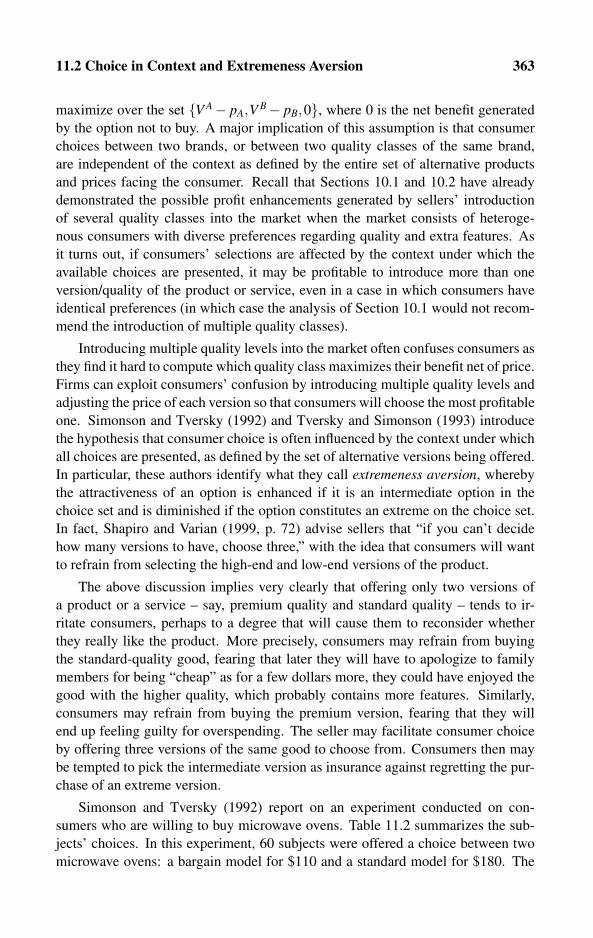
11.2 Choice in Context and Extremeness Aversion 363
maximize over the set {V A− pA,V B− pB,0}, where 0 is the net benefit generated
by the option not to buy. A major implication of this assumption is that consumer
choices between two brands, or between two quality classes of the same brand,
are independent of the context as defined by the entire set of alternative products
and prices facing the consumer. Recall that Sections 10.1 and 10.2 have already
demonstrated the possible profit enhancements generated by sellers’ introduction
of several quality classes into the market when the market consists of heteroge-
nous consumers with diverse preferences regarding quality and extra features. As
it turns out, if consumers’ selections are affected by the context under which the
available choices are presented, it may be profitable to introduce more than one
version/quality of the product or service, even in a case in which consumers have
identical preferences (in which case the analysis of Section 10.1 would not recom-
mend the introduction of multiple quality classes).
Introducing multiple quality levels into the market often confuses consumers as
they find it hard to compute which quality class maximizes their benefit net of price.
Firms can exploit consumers’ confusion by introducing multiple quality levels and
adjusting the price of each version so that consumers will choose the most profitable
one. Simonson and Tversky (1992) and Tversky and Simonson (1993) introduce
the hypothesis that consumer choice is often influenced by the context under which
all choices are presented, as defined by the set of alternative versions being offered.
In particular, these authors identify what they call extremeness aversion, whereby
the attractiveness of an option is enhanced if it is an intermediate option in the
choice set and is diminished if the option constitutes an extreme on the choice set.
In fact, Shapiro and Varian (1999, p. 72) advise sellers that “if you can’t decide
how many versions to have, choose three,” with the idea that consumers will want
to refrain from selecting the high-end and low-end versions of the product.
The above discussion implies very clearly that offering only two versions of
a product or a service – say, premium quality and standard quality – tends to ir-
ritate consumers, perhaps to a degree that will cause them to reconsider whether
they really like the product. More precisely, consumers may refrain from buying
the standard-quality good, fearing that later they will have to apologize to family
members for being “cheap” as for a few dollars more, they could have enjoyed the
good with the higher quality, which probably contains more features. Similarly,
consumers may refrain from buying the premium version, fearing that they will
end up feeling guilty for overspending. The seller may facilitate consumer choice
by offering three versions of the same good to choose from. Consumers then may
be tempted to pick the intermediate version as insurance against regretting the pur-
chase of an extreme version.
Simonson and Tversky (1992) report on an experiment conducted on con-
sumers who are willing to buy microwave ovens. Table 11.2 summarizes the sub-
jects’ choices. In this experiment, 60 subjects were offered a choice between two
microwave ovens: a bargain model for $110 and a standard model for $180. The
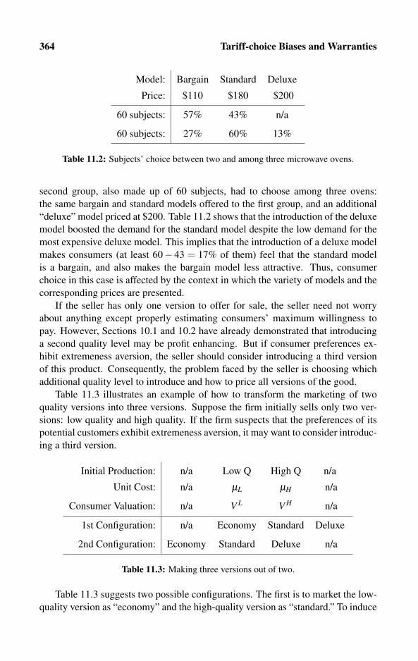
364 Tariff-choice Biases and Warranties
Model: Bargain Standard Deluxe
Price: $110 $180 $200
60 subjects: 57% 43% n/a
60 subjects: 27% 60% 13%
Table 11.2: Subjects’ choice between two and among three microwave ovens.
second group, also made up of 60 subjects, had to choose among three ovens:
the same bargain and standard models offered to the first group, and an additional
“deluxe” model priced at $200. Table 11.2 shows that the introduction of the deluxe
model boosted the demand for the standard model despite the low demand for the
most expensive deluxe model. This implies that the introduction of a deluxe model
makes consumers (at least 60− 43 = 17% of them) feel that the standard model
is a bargain, and also makes the bargain model less attractive. Thus, consumer
choice in this case is affected by the context in which the variety of models and the
corresponding prices are presented.
If the seller has only one version to offer for sale, the seller need not worry
about anything except properly estimating consumers’ maximum willingness to
pay. However, Sections 10.1 and 10.2 have already demonstrated that introducing
a second quality level may be profit enhancing. But if consumer preferences ex-
hibit extremeness aversion, the seller should consider introducing a third version
of this product. Consequently, the problem faced by the seller is choosing which
additional quality level to introduce and how to price all versions of the good.
Table 11.3 illustrates an example of how to transform the marketing of two
quality versions into three versions. Suppose the firm initially sells only two ver-
sions: low quality and high quality. If the firm suspects that the preferences of its
potential customers exhibit extremeness aversion, it may want to consider introduc-
ing a third version.
Initial Production: n/a Low Q High Q n/a
Unit Cost: n/a μL μH n/a
Consumer Valuation: n/a V L V H n/a
1st Configuration: n/a Economy Standard Deluxe
2nd Configuration: Economy Standard Deluxe n/a
Table 11.3: Making three versions out of two.
Table 11.3 suggests two possible configurations. The first is to market the low-
quality version as “economy” and the high-quality version as “standard.” To induce
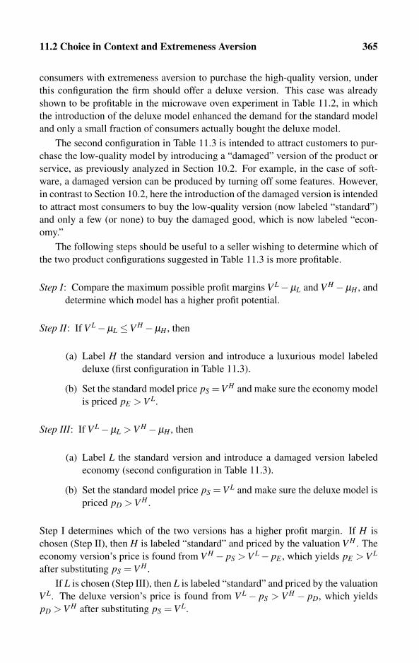
11.2 Choice in Context and Extremeness Aversion 365
consumers with extremeness aversion to purchase the high-quality version, under
this configuration the firm should offer a deluxe version. This case was already
shown to be profitable in the microwave oven experiment in Table 11.2, in which
the introduction of the deluxe model enhanced the demand for the standard model
and only a small fraction of consumers actually bought the deluxe model.
The second configuration in Table 11.3 is intended to attract customers to pur-
chase the low-quality model by introducing a “damaged” version of the product or
service, as previously analyzed in Section 10.2. For example, in the case of soft-
ware, a damaged version can be produced by turning off some features. However,
in contrast to Section 10.2, here the introduction of the damaged version is intended
to attract most consumers to buy the low-quality version (now labeled “standard”)
and only a few (or none) to buy the damaged good, which is now labeled “econ-
omy.”
The following steps should be useful to a seller wishing to determine which of
the two product configurations suggested in Table 11.3 is more profitable.
Step I: Compare the maximum possible profit margins V L−μL and V H −μH , and
determine which model has a higher profit potential.
Step II: If V L−μL ≤V H −μH , then
(a) Label H the standard version and introduce a luxurious model labeled
deluxe (first configuration in Table 11.3).
(b) Set the standard model price pS =V H and make sure the economy model
is priced pE > V L.
Step III: If V L−μL > V H −μH , then
(a) Label L the standard version and introduce a damaged version labeled
economy (second configuration in Table 11.3).
(b) Set the standard model price pS = V L and make sure the deluxe model is
priced pD > V H .
Step I determines which of the two versions has a higher profit margin. If H is
chosen (Step II), then H is labeled “standard” and priced by the valuation V H . The
economy version’s price is found from V H − pS > V L− pE , which yields pE > V L
after substituting pS = V H .
If L is chosen (Step III), then L is labeled “standard” and priced by the valuation
V L. The deluxe version’s price is found from V L− pS > V H − pD, which yields
pD > V H after substituting pS = V L.

366 Tariff-choice Biases and Warranties
11.3 Other Consumer Choice Biases
Section 11.1 analyzed consumer biases toward flat-rate payment plans. Section 11.2
analyzed consumer biases against high- and low-end versions of products and ser-
vices in the form of extremeness aversion. This section briefly discusses a few
additional biases that are often observed when reviewing consumers’ selections
among brands, quality levels, and prices.
11.3.1 Odd pricing and the 99/c fixation
It is widely observed that most retailers in the United States price products and
services to end in 99/c. This pricing structure is often referred to as the 9 fixation.
The scientific literature, such as Basu (1997), Schindler and Kirby (1997), Stiving
and Winer (1997), and Thomas and Morwitz (2005), proposed several explanations
for this observation.
Rounding illusions: Consumers tend to approximate the prices they pay by a lower
integer or a lower decimal number rather than by a higher one. Thus, de-
pending on the level of rounding numbers, consumers may state or report
a price of $999.99 as nine-hundred-ninety-nine, or as nine-hundred-ninety,
or simply nine-hundred dollars. This means that people tend to underquote
a price according to the leading digits of the price. Stores, then, maximize
profit by setting the last digits as large as possible, in which case they simply
add the relevant sequence of 9s.
Consumers like to receive change: Therefore, if stores take into their pricing con-
sideration the assumption that consumers’ utility is enhanced by receiving
change, they will maximize profit by handing out the minimum-possible
change, which is 1/c. Hence, all prices end with 99/c.
Attractive digits: People find the combinations of 99, 999, 9999, and so on, to be
“nice.” Thus, consumers are attracted to prices involving many digits of nine.
Hence, this “elegant” statement of the price serves as a store-advertising
mechanism because after looking at the price itself, consumers are more
likely to pay attention to other details and features of the good offered by
this seller.
Image of a discount retailer: Discount stores tend to use black-and-white ads to
create an image that the store is engaged in significant cost cutting. Similarly,
a price of 99/c may indicate that a store is concerned with all levels of cost
cutting and that even a 1/c cost reduction is being transferred to the consumers
in the form of a 1/c price reduction.
Agency problem and theft: With the absence of on-the-job cameras, owners have
no way of ensuring that cashiers collect and transfer the proceeds from all
11.3 Other Consumer Choice Biases 367
sales. A price of $5.00 means that too many customers will hand over exactly
one $5 bill or five $1 bills without waiting for the sale to be rung on the
machine. In this case, the cashier can pocket the cash without having to
register the transaction. In contrast, a price of $4.99 forces the customer to
wait to receive change and the employee to register the transaction to be able
to hand out the 1/c change.
Finally, there is a question regarding the 99/c pricing structure is only an Amer-
ican phenomenon. As it turns out, although 99/c prices are perhaps more visible in
the United States, more and more stores in other countries are adopting this pricing
structure. Thus, it remains to be seen whether the 99/c component of the price trans-
lates into different currencies with different purchasing power. Gabor and Granger
(1966) and Gabor (1988, pp. 258–259) report on prices of nylon stockings in Eng-
land prior to decimalization of the currency. Their striking result is presented on
a graph of potential consumers as a function of price and shows that the patterns
of no change in potential consumers lie in ranges between prices having the same
shilling components, such as 2 shillings and 10 pence, and 2 shillings and 11 pence.
Stating it differently, the steepest drops in the buy responses were found when the
price changed from 5 shillings and 11 pence to 6 shillings and 0 pence, or any sim-
ilar changes from 6/11 to 7/–, 7/11 to 8/–, 8/11 to 9/–, and so on. Using Gabor’s
words, “this price structure has become imprinted on the customers’ minds and has
found clear expression in their responses.”
11.3.2 Price–quality perceptions
It is well known that consumers attach value to the way in which the product is
packaged. This is, of course, very strange because packages tend to be thrown
away after the consumer starts using the product. For some reason, the quality of
the box serves as a signal for the quality of the product. In exactly the same way,
consumers perceive the price itself as a signal.
The reader has probably heard many people say “there must be something
wrong with this product because it is priced so low.” Thus, many consumers be-
lieve that within each group of products and services, the quality of the good is
somewhat reflected by its price level. This belief on the part of consumers explains
why some consumers place a lower bound on the price below which they will reject
a price offer in addition to an upper bound beyond which they will also not buy, as
they view it as “too expensive.” Gabor and Granger (1966) discuss two methods for
surveying consumers’ reactions to price offers. The first method involves two ques-
tions: one asking for the highest price at which the consumer would buy and the
second asking for the lowest price. The second method asks consumers to respond
to a list of prices for a certain item by stating whether they would buy, whether they
would not buy because the price is too high, or whether they would not buy because
the price is too low. A reader who cannot rationalize a behavior under which a con-
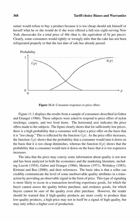
368 Tariff-choice Biases and Warranties
sumer would refuse to buy a product because it is too cheap should ask himself or
herself what he or she would do if she were offered a full-size eight-serving New
York cheesecake for a total price of 40/c (that is, the equivalent of 5/c per piece).
Clearly, some consumers would rightly or wrongly infer that the cake has not been
refrigerated properly or that the last date of sale has already passed.
�
�
p
Probability
00
1h(p)
�(p)
Figure 11.1: Consumer responses to price offers.
Figure 11.1 displays the results from a sample of consumers described in Gabor
and Granger (1966). These subjects were asked to respond to price offers of nylon
stockings, carpets, and two food items. The horizontal axis indicates the price
offers made to the subjects. The figure clearly shows that for sufficiently low prices,
there is a high probability that a consumer will reject a price offer on the basis that
it is “too cheap.” This is reflected by the function �(p). As the price offer increases,
the function �(p) shows that the probability that a consumer would turn it down on
the basis that it is too cheap diminishes, whereas the function h(p) shows that the
probability that a consumer would turn it down on the basis that it is too expensive
increases.
The idea that the price may convey some information about quality is not new
and has been analyzed in both the economics and the marketing literature, includ-
ing Leavitt (1954), Gabor and Granger (1966), Monroe (1971), Wolinksy (1983),
Kirmani and Rao (2000), and their references. The basic idea is that a seller can
credibly communicate the level of some unobservable quality attributes in a trans-
action by providing an observable signal in the form of price. This type of signaling
is more likely to occur in a transaction involving experience goods, for which the
buyer cannot assess the quality before purchase, and credence goods, for which
buyers cannot be sure of the quality even after purchase. However, the reader
should be warned that if high-quality products are more costly to produce than
low-quality products, a high price may not in itself be a signal of high quality, but
may only reflect a higher cost of production.

11.4 Warranties 369
11.3.3 Micropayments and currency denomination
Many consumers are biased toward buying items priced by small currency denom-
inations. The desire for small payments gave rise to the 99/c stores in the United
States, and more recently, to the e1 stores now widely observed in major European
cities. In addition, the widespread use of the Internet for commerce in general, and
for trade in information goods in particular, as well as the digital convergence of
text, image, audio, and video formats has opened up new ways of transacting in
“small portions” for low prices. For example, instead of buying a full-album CD
for e13, consumers can now purchase one song for 99/c by downloading it directly
from the Internet. Clearly, this type of “unbundling” was not possible before this
change in technology, as both transportation and data storage costs made it pro-
hibitively costly to market one song at a time.
Another common way of making the price look smaller is to split the transac-
tion into several currencies. Passengers traveling through European airports may
recall duty-free shops that are willing to accept multiple currencies for small pur-
chases, such as a piece of chocolate or a bottle of whiskey. Travelers generally use
these stores to “get rid” of their unused currencies. Dreze and Nunes (2004) ex-
plore how consumers evaluate transactions that involve combined-currency prices,
and prices stated in multiple, relatively new currencies. Some of these new curren-
cies were introduced by loyalty programs and related marketing promotions such
as frequent-flier miles and credit card rewards in the form of points that consumers
accumulate and then spend as they do traditional forms of money. As a result, con-
sumers are increasingly able to pay for goods and services such as airline travel,
hotel stays, and groceries in various combinations of traditional and new curren-
cies. These combined-currency prices are widely visible in the form of prices such
as $39 and 16,000 miles gained from air travel or points gained via financial prod-
ucts such as brand-name credit cards. This pricing technique seems to be lowering
consumers’ psychological cost and perceived price associated with a particular pur-
chase.
11.4 Warranties
Warranties provide insurance for consumers that consumers tend to value. In fact,
it is often observed that warranties are priced higher than the expected loss they
insure against. Moreover, stores selling electronic appliances tend to offer their own
supplementary warranties in addition to the warranty supplied by the manufacturer.
Consumers who buy them end up purchasing two warranties for the same product.
The above discussion implies that consumers tend to value warranties not only
because warranties insure against a loss associated with a defective product or an
improperly delivered service, but also because warranties provide some psychologi-
cal comfort. Therefore, although the present analysis computes the maximum price
370 Tariff-choice Biases and Warranties
a seller can charge for a warranty on the basis of insurance only, the reader should
view this warranty price as a lower bound on this price because many consumers
would be willing to pay a higher price for the psychological comfort associated
with having a warranty, which is not captured by the following computations. In
fact, the analysis of warranties is somewhat related to the analysis of refunds (see
Chapter 8) as refunds also provide some psychological comfort in the form of in-
surance against no-shows. However, the difference between warranties and refunds
is that warranties insure against defective products and services, whereas refunds
also insure against consumer no-shows (in which case consumers buy “insurance”
against their own uncertainty).
The analysis of warranties in this book abstracts from two important aspects.
The first is moral hazard behavior in which consumers are not careful in operating
the product, which could lead to a higher failure rate. The effects of moral hazard
can be somewhat mitigated if the warranties state that they do not cover any misuse
of the product. The second aspect that is not analyzed in this short presentation is
adverse selection, which may occur if the seller offers the warranty as an option
rather than as a tied-in feature. In this case, it may happen that consumers who are
likely to abuse the product will choose to buy the warranty, whereas “responsible”
consumers will choose not to buy the warranty. Again, a proper warning by the
seller that misuse voids the warranty would help in mitigating this effect.
The analysis below assumes that a seller offers a product for sale that may be
either fully functional or totally defective, but nothing in between. The exact con-
dition of each product is not known to the seller or to the potential buyers, but the
probability that the product is fully functional is common knowledge. Let π denote
the probability that the product in question is fully functional, 0 ≤ π ≤ 1. Hence,
each product is defective with probability 1−π . There are N potential customers.
Consumers’ maximum willingness to pay is $V > 0 for a fully functional product
and 0 for a defective product. Let μ denote the unit production cost of this prod-
uct and φ the fixed cost. Finally, it must be verified that the expected benefit to a
consumer exceeds the marginal production cost, as otherwise this product cannot
be profitable. Formally, these parameters should satisfy πV ≥ μ .
11.4.1 Product replacement warranties
A product replacement warranty is a contract between a seller (or a manufacturer)
and a buyer promising the buyer to replace a defective product with a new product.
However, buyers should ask themselves what happens if the replacement product
also fails, and then what happens if the replacement of the replacement product
fails, and so on. For this reason, the analysis of product replacement warranties is
conducted under various configurations of replacement possibilities.
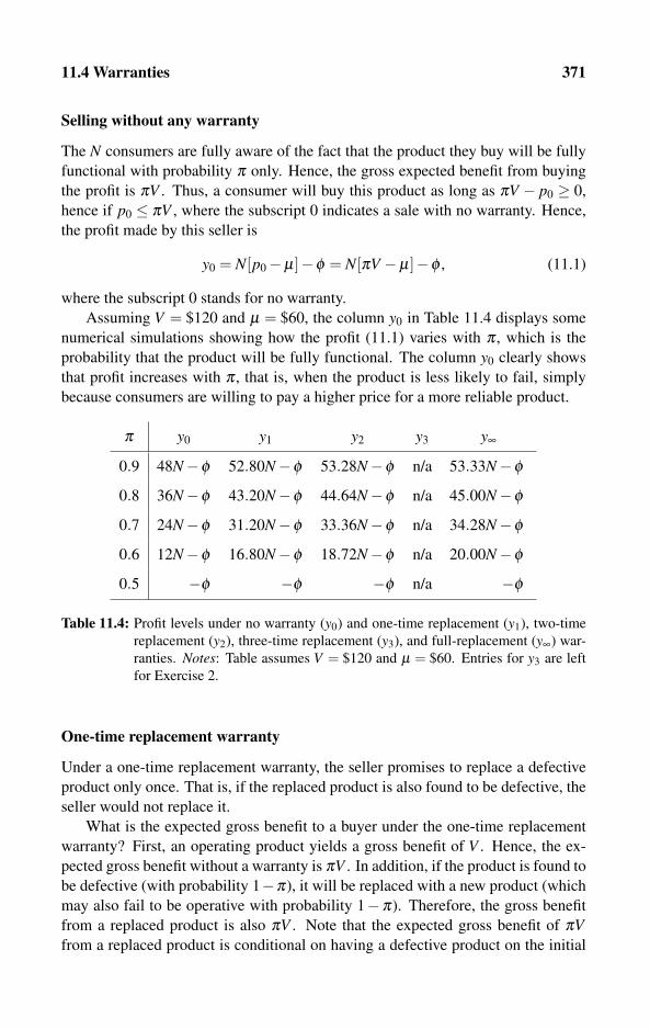
11.4 Warranties 371
Selling without any warranty
The N consumers are fully aware of the fact that the product they buy will be fully
functional with probability π only. Hence, the gross expected benefit from buying
the profit is πV . Thus, a consumer will buy this product as long as πV − p0 ≥ 0,
hence if p0 ≤ πV , where the subscript 0 indicates a sale with no warranty. Hence,
the profit made by this seller is
y0 = N[p0−μ]−φ = N[πV −μ]−φ , (11.1)
where the subscript 0 stands for no warranty.
Assuming V = $120 and μ = $60, the column y0 in Table 11.4 displays some
numerical simulations showing how the profit (11.1) varies with π , which is the
probability that the product will be fully functional. The column y0 clearly shows
that profit increases with π , that is, when the product is less likely to fail, simply
because consumers are willing to pay a higher price for a more reliable product.
π y0 y1 y2 y3 y∞
0.9 48N−φ 52.80N−φ 53.28N−φ n/a 53.33N−φ
0.8 36N−φ 43.20N−φ 44.64N−φ n/a 45.00N−φ
0.7 24N−φ 31.20N−φ 33.36N−φ n/a 34.28N−φ
0.6 12N−φ 16.80N−φ 18.72N−φ n/a 20.00N−φ
0.5 −φ −φ −φ n/a −φ
Table 11.4: Profit levels under no warranty (y0) and one-time replacement (y1), two-time
replacement (y2), three-time replacement (y3), and full-replacement (y∞) war-
ranties. Notes: Table assumes V = $120 and μ = $60. Entries for y3 are left
for Exercise 2.
One-time replacement warranty
Under a one-time replacement warranty, the seller promises to replace a defective
product only once. That is, if the replaced product is also found to be defective, the
seller would not replace it.
What is the expected gross benefit to a buyer under the one-time replacement
warranty? First, an operating product yields a gross benefit of V . Hence, the ex-
pected gross benefit without a warranty is πV . In addition, if the product is found to
be defective (with probability 1−π), it will be replaced with a new product (which
may also fail to be operative with probability 1−π). Therefore, the gross benefit
from a replaced product is also πV . Note that the expected gross benefit of πVfrom a replaced product is conditional on having a defective product on the initial
372 Tariff-choice Biases and Warranties
purchase, and this happens with probability 1−π . Hence, the total expected gross
benefit from a product sold with a one-time replacement warranty is
πV︸︷︷︸Original purchase
+ (1−π)πV︸ ︷︷ ︸Replacement
= (2−π)πV. (11.2)
What would be the expected cost to the seller (or the manufacturer), given that
each unit costs μ to produce? The initial sale costs μ . But the customer will
demand a replacement product with probability (1−π). Hence, the total expected
production cost borne by the seller or the manufacturer is
c1 = N [ μ︸︷︷︸Original
+ (1−π)μ︸ ︷︷ ︸Replacement
]−φ = N(2−π)μ−φ , (11.3)
where the subscript 1 stands for one-time replacement.
Recall that (11.2) provides consumers’ maximum willingness to pay for a prod-
uct with a one-time replacement warranty. Thus, a monopoly seller should set the
price p1 = (2−π)πV . Therefore, total profit under a one-time replacement war-
ranty is given by
y1 = N p1− c1 = N(2−π)(πV −μ)−φ . (11.4)
Column y1 in Table 11.4 displays some numerical simulations showing how the
profit (11.4) varies with π , which is the probability that the product will be fully
functional. Column y1 clearly shows that profit increases with π , that is, when the
product is less likely to fail.
Two-time replacement warranty
The total expected gross benefit from a product sold with a two-time replacement
warranty is
πV︸︷︷︸Original purchase
+ (1−π)πV︸ ︷︷ ︸1st replacement
+ (1−π)2πV︸ ︷︷ ︸2nd replacement
= (π2−3π +3)πV. (11.5)
That is, the product fails twice with probability (1−π)2. This has to be multiplied
by the expected benefit from the second and last replacement πV .
The expected production cost to the seller (or the manufacturer) is
c2 = N[ μ︸︷︷︸Original
+ (1−π)μ︸ ︷︷ ︸1st replacement
+ (1−π)2μ︸ ︷︷ ︸2nd replacement
]
= N(π2−3π +3)μ−φ , (11.6)
where the subscript 2 stands for two-time replacement. The gross benefit (11.5)
implies that a monopoly seller would set the price p2 = (π2− 3π + 3)πV for a
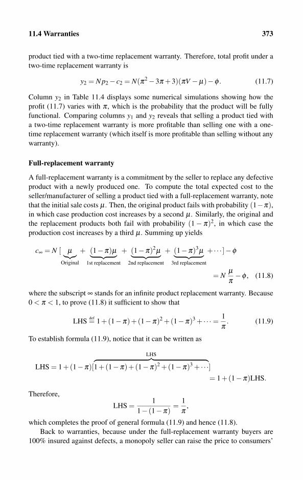
11.4 Warranties 373
product tied with a two-time replacement warranty. Therefore, total profit under a
two-time replacement warranty is
y2 = N p2− c2 = N(π2−3π +3)(πV −μ)−φ . (11.7)
Column y2 in Table 11.4 displays some numerical simulations showing how the
profit (11.7) varies with π , which is the probability that the product will be fully
functional. Comparing columns y1 and y2 reveals that selling a product tied with
a two-time replacement warranty is more profitable than selling one with a one-
time replacement warranty (which itself is more profitable than selling without any
warranty).
Full-replacement warranty
A full-replacement warranty is a commitment by the seller to replace any defective
product with a newly produced one. To compute the total expected cost to the
seller/manufacturer of selling a product tied with a full-replacement warranty, note
that the initial sale costs μ . Then, the original product fails with probability (1−π),in which case production cost increases by a second μ . Similarly, the original and
the replacement products both fail with probability (1− π)2, in which case the
production cost increases by a third μ . Summing up yields
c∞ = N [ μ︸︷︷︸Original
+ (1−π)μ︸ ︷︷ ︸1st replacement
+ (1−π)2μ︸ ︷︷ ︸2nd replacement
+ (1−π)3μ︸ ︷︷ ︸3rd replacement
+ · · · ]−φ
= Nμπ−φ , (11.8)
where the subscript ∞ stands for an infinite product replacement warranty. Because
0 < π < 1, to prove (11.8) it sufficient to show that
LHSdef= 1+(1−π)+(1−π)2 +(1−π)3 + · · ·= 1
π. (11.9)
To establish formula (11.9), notice that it can be written as
LHS = 1+(1−π)[
LHS︷ ︸︸ ︷1+(1−π)+(1−π)2 +(1−π)3 + · · ·]
= 1+(1−π)LHS.
Therefore,
LHS =1
1− (1−π)=
1
π,
which completes the proof of general formula (11.9) and hence (11.8).
Back to warranties, because under the full-replacement warranty buyers are
100% insured against defects, a monopoly seller can raise the price to consumers’
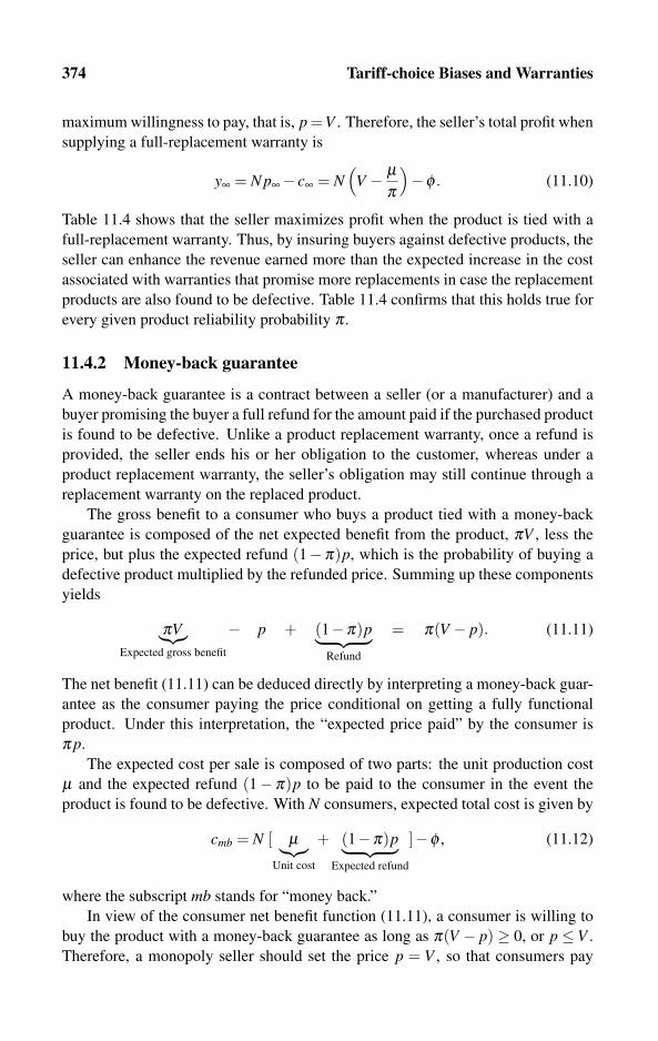
374 Tariff-choice Biases and Warranties
maximum willingness to pay, that is, p =V . Therefore, the seller’s total profit when
supplying a full-replacement warranty is
y∞ = N p∞− c∞ = N(
V − μπ
)−φ . (11.10)
Table 11.4 shows that the seller maximizes profit when the product is tied with a
full-replacement warranty. Thus, by insuring buyers against defective products, the
seller can enhance the revenue earned more than the expected increase in the cost
associated with warranties that promise more replacements in case the replacement
products are also found to be defective. Table 11.4 confirms that this holds true for
every given product reliability probability π .
11.4.2 Money-back guarantee
A money-back guarantee is a contract between a seller (or a manufacturer) and a
buyer promising the buyer a full refund for the amount paid if the purchased product
is found to be defective. Unlike a product replacement warranty, once a refund is
provided, the seller ends his or her obligation to the customer, whereas under a
product replacement warranty, the seller’s obligation may still continue through a
replacement warranty on the replaced product.
The gross benefit to a consumer who buys a product tied with a money-back
guarantee is composed of the net expected benefit from the product, πV , less the
price, but plus the expected refund (1−π)p, which is the probability of buying a
defective product multiplied by the refunded price. Summing up these components
yields
πV︸︷︷︸Expected gross benefit
− p + (1−π)p︸ ︷︷ ︸Refund
= π(V − p). (11.11)
The net benefit (11.11) can be deduced directly by interpreting a money-back guar-
antee as the consumer paying the price conditional on getting a fully functional
product. Under this interpretation, the “expected price paid” by the consumer is
π p.
The expected cost per sale is composed of two parts: the unit production cost
μ and the expected refund (1− π)p to be paid to the consumer in the event the
product is found to be defective. With N consumers, expected total cost is given by
cmb = N [ μ︸︷︷︸Unit cost
+ (1−π)p︸ ︷︷ ︸Expected refund
]−φ , (11.12)
where the subscript mb stands for “money back.”
In view of the consumer net benefit function (11.11), a consumer is willing to
buy the product with a money-back guarantee as long as π(V − p) ≥ 0, or p ≤ V .
Therefore, a monopoly seller should set the price p = V , so that consumers pay

11.5 Exercises 375
a price equal to their gross benefit from a fully functioning product. Hence, the
expected total profit of this seller is
ymb = N p−N[μ +(1−π)p]−φ = NV −N[μ +(1−π)V ]−φ= N(πV −μ)−φ . (11.13)
Comparing (11.13) with (11.1) reveals that the profit earned from selling the prod-
uct tied with a money-back guarantee is identical to the profit from selling without
any warranty. Whereas under no warranty the seller must lower the price to πV to
attract the consumer to buy a product that is defective with probability 1− π , in
doing so the seller shifts all the risk to the consumer. In contrast, under a money-
back guarantee, the seller bears the entire risk, which explains why the price can
be raised to consumers’ maximum willingness to pay for a nondefective product.
Because the seller and the buyers are assumed to be risk neutral, the transfer of the
financial risk exactly offsets the change in price, which leaves the seller with the
same profit. It should be noted that this result may not hold for risk-averse sellers
and buyers.
The overall recommendation that comes out of our analysis of warranties is that
risk-neutral sellers facing risk-neutral buyers should avoid money-back guarantees
and instead provide product replacement warranties. However, it should be noted
that because money-back guarantees are often observed, they may serve some pur-
pose for the seller after all. One possibility is that sellers in general, and large retail
stores in particular, often test new products. To avoid large spending on testing the
products before putting them on the shelves, retail stores can use their customer
base to test their products by offering them full refunds. Clearly, in this case a
money-back guarantee may end up being more profitable than a full-replacement
warranty, especially for newly marketed products that have not been tested before.
11.5 Exercises
1. The transportation authority of the City of Berlin (BVG) offers a monthly
pass for f = e67 (actual data for 2007). A one-way U-Bahn/bus ticket costs
p = e2.10. Let q denote the monthly number of trips. Mr. Merkel always uses
a monthly pass. If Mr. Merkel makes an average of q = 30 rides each month,
can you tell whether he has a flat-rate bias?
2. Consider a three-time replacement warranty in which the seller commits to re-
placing a defective product with a new one, replacing the replacement if found
to be defective, and replacing the replacement of the replacement, but no more.
Using the analysis of Section 11.4.1 solve the following problems.
(a) Similar to the formulation of price, cost, and profit for the two-time re-
placement warranty given by (11.5), (11.6), and (11.7), compute the gen-

376 Tariff-choice Biases and Warranties
eral formulation of price, cost, and profit under the three-time replacement
warranty.
(b) Fill in the missing entries for Column y3 in Table 11.4. Explain how the
profit y3 varies with an increase in the probability that the product is fully
functional π .
3. Suppose that the seller offers a “half” money-back guarantee if the product is
found to be defective after it is sold to a consumer. More precisely, if the con-
sumer pays a price of $p, the seller promises to refund the consumer with $p/2
in the event the product happens to be defective. Using the analysis of Sec-
tion 11.4.2 solve the following problems.
(a) Similar to the formulation of price, cost, and profit for the “full” money-
back guarantee given by (11.11), (11.12), and (11.13), compute the general
formulation of price, cost, and profit for the half money-back guarantee.
(b) Compare the profit you just computed for the half refund guarantee, with
the profit earned when the seller offers a full money-back guarantee given
by (11.13). Explain the difference (if any).

Chapter 12
Instructor and Solution Manual
12.1 To the Reader
There are two main purposes for adding this extra chapter.
(a) To provide abbreviated solutions for all exercises appearing at the end of each
chapter.
(b) To provide some suggestions to instructors and to the general reader regarding
which topics to emphasize, and to comment on the general logic behind the
specific ordering of the topics covered in each chapter.
I emphasize abbreviated solutions because I see no need to repeat all the steps
developed in the body of each chapter. All I want is to provide the reader with some
feedback on whether they can independently solve the kind of problems analyzed
in this book. However, students should be required to submit their homework in
greater detail than that given in this manual, using all the steps developed in the
body of each chapter.
Some instructors may not like the fact that the solutions for all exercises are
provided as this will require them to write more exercises for homework and exam
purposes. However, I can assure the instructors that even if they do not assign any
formal homework, students will learn much better if they can train themselves by
looking at the solutions to the problems they are supposed to know how to solve. In
fact, in the past, I ended up placing the solutions for all the problem sets that appear
in my previous two textbooks on my Web page, www.ozshy.com, simply because
I realized that students perform much better in exams after reading the proposed
solutions.
As for the book itself, I tried to separate the chapters to make them as inde-
pendent of each other as possible. This means that the instructor as well as the
general reader can choose to teach or study whatever topics he or she wishes with-
out having to follow a long sequence of chapters as a preparation for a certain topic.
Regardless, I have tried my best to use consistent notation throughout this book (see
Table 1.4).
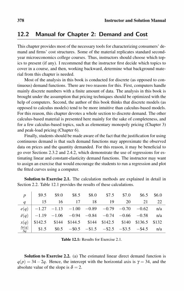
378 Instructor and Solution Manual
12.2 Manual for Chapter 2: Demand and Cost
This chapter provides most of the necessary tools for characterizing consumers’ de-
mand and firms’ cost structures. Some of the material replicates standard second-
year microeconomics college courses. Thus, instructors should choose which top-
ics to present (if any). I recommend that the instructor first decide which topics to
cover in a course, and then, working backward, determine what background mate-
rial from this chapter is needed.
Most of the analysis in this book is conducted for discrete (as opposed to con-
tinuous) demand functions. There are two reasons for this. First, computers handle
mainly discrete numbers with a finite amount of data. The analysis in this book is
brought under the assumption that pricing techniques should be optimized with the
help of computers. Second, the author of this book thinks that discrete models (as
opposed to calculus models) tend to be more intuitive than calculus-based models.
For this reason, this chapter devotes a whole section to discrete demand. The other
calculus-based material is presented here mainly for the sake of completeness, and
for a few calculus-based topics, such as elementary monopoly pricing (Chapter 3)
and peak-load pricing (Chapter 6).
Finally, students should be made aware of the fact that the justification for using
continuous demand is that such demand functions may approximate the observed
data on prices and the quantity demanded. For this reason, it may be beneficial to
go over Sections 2.3.2 and 2.4.2, which demonstrate the use of regressions for es-
timating linear and constant-elasticity demand functions. The instructor may want
to assign an exercise that would encourage the students to run a regression and plot
the fitted curves using a computer.
Solution to Exercise 2.1. The calculation methods are explained in detail in
Section 2.2. Table 12.1 provides the results of these calculations.
p $9.5 $9.0 $8.5 $8.0 $7.5 $7.0 $6.5 $6.0
q 15 16 17 18 19 20 21 22
e(q) −1.27 −1.13 −1.00 −0.89 −0.79 −0.70 −0.62 n/a
e(q) −1.19 −1.06 −0.94 −0.84 −0.74 −0.66 −0.58 n/a
x(q) $142.5 $144 $144.5 $144 $142.5 $140 $136.5 $132Δx(q)
Δq $1.5 $0.5 −$0.5 −$1.5 −$2.5 −$3.5 −$4.5 n/a
Table 12.1: Results for Exercise 2.1.
Solution to Exercise 2.2. (a) The estimated linear direct demand function is
q(p) = 34− 2q. Hence, the intercept with the horizontal axis is γ = 34, and the
absolute value of the slope is δ = 2.

12.2 Manual for Chapter 2: Demand and Cost 379
(b) The corresponding direct demand function is p(q) = 17−0.5p.
(c) Running the linear regression lnq = lnα −β ln p on a computer yields lnα =5.50 and −β =−1.19. Hence, q(p) = 244.89 p−1.19.
(d) The price elasticity of a constant-elasticity demand function equals the exponent
of the price. Hence, e(p) =−1.19. Because |e(p)|> 1, the demand is elastic.
Solution to Exercise 2.3. (a) The inverse demand function is given by p =17−0.5q. The revenue function is x(q) def= p(q)q = (34−q)q/2.
(b) Using calculus to solve maxq x(q), the first- and second-order conditions for a
maximum are
0 =dp(q)q
dq= 17−q, and
d2 p(q)qdq2
=−q < 0,
for every output level q > 0. Hence, q = 17 is the revenue-maximizing output level,
and p = 34−17 = $17 is the corresponding revenue-maximizing price.
(c) The revenue level evaluated at the revenue-maximizing output is x(17) = (34−17)17/2 = $144.5. The price elasticity is
e(q) =dq(p)
dppq
=−217−0.5q
q=−2
17−0.5 ·17
17=−1.
As expected, revenue is maximized at the output level associated with a unit price
elasticity.
Solution to Exercise 2.4. Horizontally adding the newly entering N4 = 200
consumers to Figure 2.8 yields the new aggregate demand function drawn in Fig-
ure 12.1.
�
p
$30
$25
$20
$15
$10
200 400 600 800 1000
•
� q1200
••
•
Figure 12.1: Aggregate demand for Exercise 2.4.
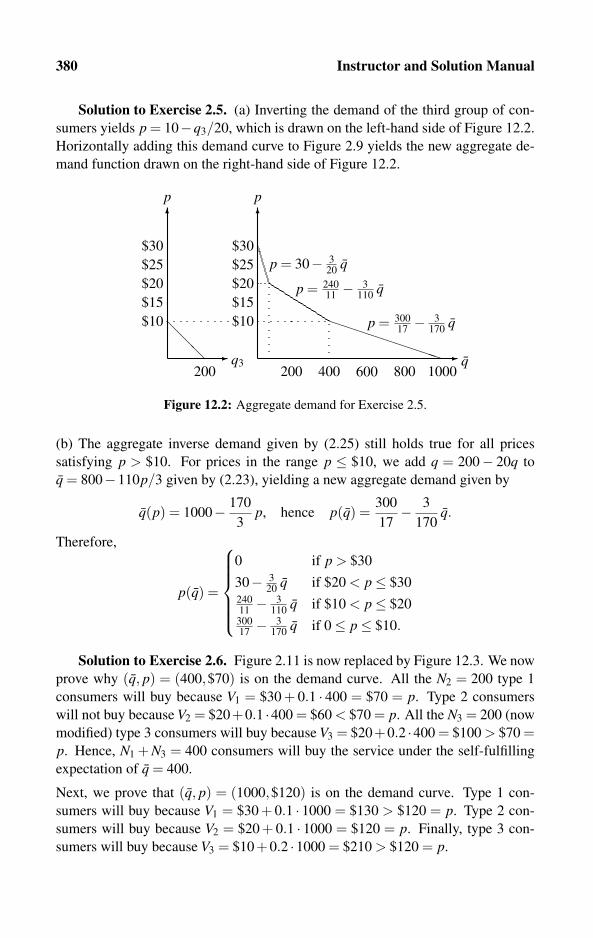
380 Instructor and Solution Manual
Solution to Exercise 2.5. (a) Inverting the demand of the third group of con-
sumers yields p = 10−q3/20, which is drawn on the left-hand side of Figure 12.2.
Horizontally adding this demand curve to Figure 2.9 yields the new aggregate de-
mand function drawn on the right-hand side of Figure 12.2.
�
p
$30
$25
$20
$15
$10
� q3200
�
p
$30
$25
$20
$15
$10
� q200 400 600 800 1000
p = 30− 320
q
���������
p = 24011− 3
110q
���
p = 30017− 3
170q
Figure 12.2: Aggregate demand for Exercise 2.5.
(b) The aggregate inverse demand given by (2.25) still holds true for all prices
satisfying p > $10. For prices in the range p ≤ $10, we add q = 200− 20q to
q = 800−110p/3 given by (2.23), yielding a new aggregate demand given by
q(p) = 1000− 170
3p, hence p(q) =
300
17− 3
170q.
Therefore,
p(q) =
⎧⎪⎪⎪⎪⎨⎪⎪⎪⎪⎩
0 if p > $30
30− 320
q if $20 < p≤ $3024011− 3
110q if $10 < p≤ $20
30017− 3
170q if 0≤ p≤ $10.
Solution to Exercise 2.6. Figure 2.11 is now replaced by Figure 12.3. We now
prove why (q, p) = (400,$70) is on the demand curve. All the N2 = 200 type 1
consumers will buy because V1 = $30 + 0.1 · 400 = $70 = p. Type 2 consumers
will not buy because V2 = $20+0.1 ·400 = $60 < $70 = p. All the N3 = 200 (now
modified) type 3 consumers will buy because V3 = $20+0.2 ·400 = $100 > $70 =p. Hence, N1 + N3 = 400 consumers will buy the service under the self-fulfilling
expectation of q = 400.
Next, we prove that (q, p) = (1000,$120) is on the demand curve. Type 1 con-
sumers will buy because V1 = $30 + 0.1 · 1000 = $130 > $120 = p. Type 2 con-
sumers will buy because V2 = $20 + 0.1 · 1000 = $120 = p. Finally, type 3 con-
sumers will buy because V3 = $10+0.2 ·1000 = $210 > $120 = p.
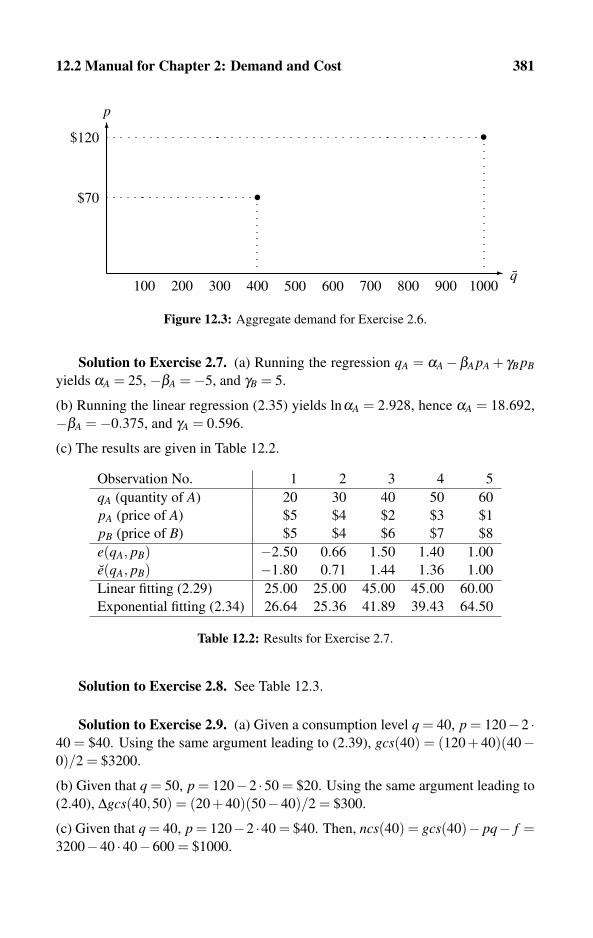
12.2 Manual for Chapter 2: Demand and Cost 381
�
�
100 200 300 400 500 600 700 800 1000900q
p
$120
$70 •
•
Figure 12.3: Aggregate demand for Exercise 2.6.
Solution to Exercise 2.7. (a) Running the regression qA = αA−βA pA + γB pB
yields αA = 25, −βA =−5, and γB = 5.
(b) Running the linear regression (2.35) yields lnαA = 2.928, hence αA = 18.692,
−βA =−0.375, and γA = 0.596.
(c) The results are given in Table 12.2.
Observation No. 1 2 3 4 5
qA (quantity of A) 20 30 40 50 60
pA (price of A) $5 $4 $2 $3 $1
pB (price of B) $5 $4 $6 $7 $8
e(qA, pB) −2.50 0.66 1.50 1.40 1.00
e(qA, pB) −1.80 0.71 1.44 1.36 1.00
Linear fitting (2.29) 25.00 25.00 45.00 45.00 60.00
Exponential fitting (2.34) 26.64 25.36 41.89 39.43 64.50
Table 12.2: Results for Exercise 2.7.
Solution to Exercise 2.8. See Table 12.3.
Solution to Exercise 2.9. (a) Given a consumption level q = 40, p = 120−2 ·40 = $40. Using the same argument leading to (2.39), gcs(40) = (120+40)(40−0)/2 = $3200.
(b) Given that q = 50, p = 120−2 ·50 = $20. Using the same argument leading to
(2.40), Δgcs(40,50) = (20+40)(50−40)/2 = $300.
(c) Given that q = 40, p = 120−2 ·40 = $40. Then, ncs(40) = gcs(40)− pq− f =3200−40 ·40−600 = $1000.
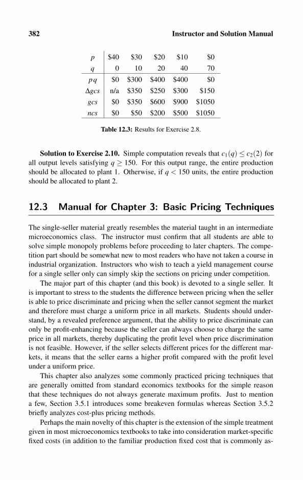
382 Instructor and Solution Manual
p $40 $30 $20 $10 $0
q 0 10 20 40 70
pq $0 $300 $400 $400 $0
Δgcs n/a $350 $250 $300 $150
gcs $0 $350 $600 $900 $1050
ncs $0 $50 $200 $500 $1050
Table 12.3: Results for Exercise 2.8.
Solution to Exercise 2.10. Simple computation reveals that c1(q) ≤ c2(2) for
all output levels satisfying q ≥ 150. For this output range, the entire production
should be allocated to plant 1. Otherwise, if q < 150 units, the entire production
should be allocated to plant 2.
12.3 Manual for Chapter 3: Basic Pricing Techniques
The single-seller material greatly resembles the material taught in an intermediate
microeconomics class. The instructor must confirm that all students are able to
solve simple monopoly problems before proceeding to later chapters. The compe-
tition part should be somewhat new to most readers who have not taken a course in
industrial organization. Instructors who wish to teach a yield management course
for a single seller only can simply skip the sections on pricing under competition.
The major part of this chapter (and this book) is devoted to a single seller. It
is important to stress to the students the difference between pricing when the seller
is able to price discriminate and pricing when the seller cannot segment the market
and therefore must charge a uniform price in all markets. Students should under-
stand, by a revealed preference argument, that the ability to price discriminate can
only be profit-enhancing because the seller can always choose to charge the same
price in all markets, thereby duplicating the profit level when price discrimination
is not feasible. However, if the seller selects different prices for the different mar-
kets, it means that the seller earns a higher profit compared with the profit level
under a uniform price.
This chapter also analyzes some commonly practiced pricing techniques that
are generally omitted from standard economics textbooks for the simple reason
that these techniques do not always generate maximum profits. Just to mention
a few, Section 3.5.1 introduces some breakeven formulas whereas Section 3.5.2
briefly analyzes cost-plus pricing methods.
Perhaps the main novelty of this chapter is the extension of the simple treatment
given in most microeconomics textbooks to take into consideration market-specific
fixed costs (in addition to the familiar production fixed cost that is commonly as-
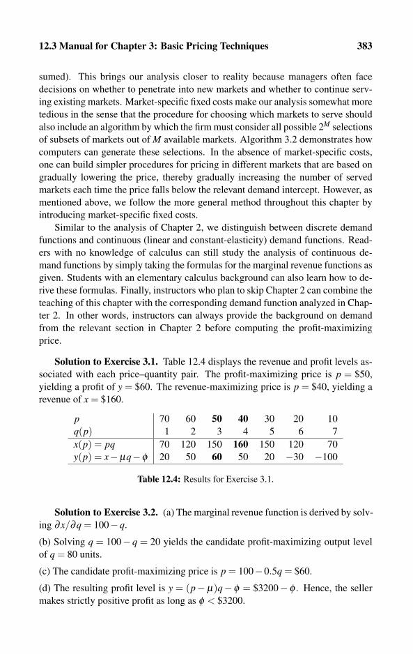
12.3 Manual for Chapter 3: Basic Pricing Techniques 383
sumed). This brings our analysis closer to reality because managers often face
decisions on whether to penetrate into new markets and whether to continue serv-
ing existing markets. Market-specific fixed costs make our analysis somewhat more
tedious in the sense that the procedure for choosing which markets to serve should
also include an algorithm by which the firm must consider all possible 2M selections
of subsets of markets out of M available markets. Algorithm 3.2 demonstrates how
computers can generate these selections. In the absence of market-specific costs,
one can build simpler procedures for pricing in different markets that are based on
gradually lowering the price, thereby gradually increasing the number of served
markets each time the price falls below the relevant demand intercept. However, as
mentioned above, we follow the more general method throughout this chapter by
introducing market-specific fixed costs.
Similar to the analysis of Chapter 2, we distinguish between discrete demand
functions and continuous (linear and constant-elasticity) demand functions. Read-
ers with no knowledge of calculus can still study the analysis of continuous de-
mand functions by simply taking the formulas for the marginal revenue functions as
given. Students with an elementary calculus background can also learn how to de-
rive these formulas. Finally, instructors who plan to skip Chapter 2 can combine the
teaching of this chapter with the corresponding demand function analyzed in Chap-
ter 2. In other words, instructors can always provide the background on demand
from the relevant section in Chapter 2 before computing the profit-maximizing
price.
Solution to Exercise 3.1. Table 12.4 displays the revenue and profit levels as-
sociated with each price–quantity pair. The profit-maximizing price is p = $50,
yielding a profit of y = $60. The revenue-maximizing price is p = $40, yielding a
revenue of x = $160.
p 70 60 50 40 30 20 10
q(p) 1 2 3 4 5 6 7
x(p) = pq 70 120 150 160 150 120 70
y(p) = x−μq−φ 20 50 60 50 20 −30 −100
Table 12.4: Results for Exercise 3.1.
Solution to Exercise 3.2. (a) The marginal revenue function is derived by solv-
ing ∂x/∂q = 100−q.
(b) Solving q = 100− q = 20 yields the candidate profit-maximizing output level
of q = 80 units.
(c) The candidate profit-maximizing price is p = 100−0.5q = $60.
(d) The resulting profit level is y = (p− μ)q− φ = $3200− φ . Hence, the seller
makes strictly positive profit as long as φ < $3200.
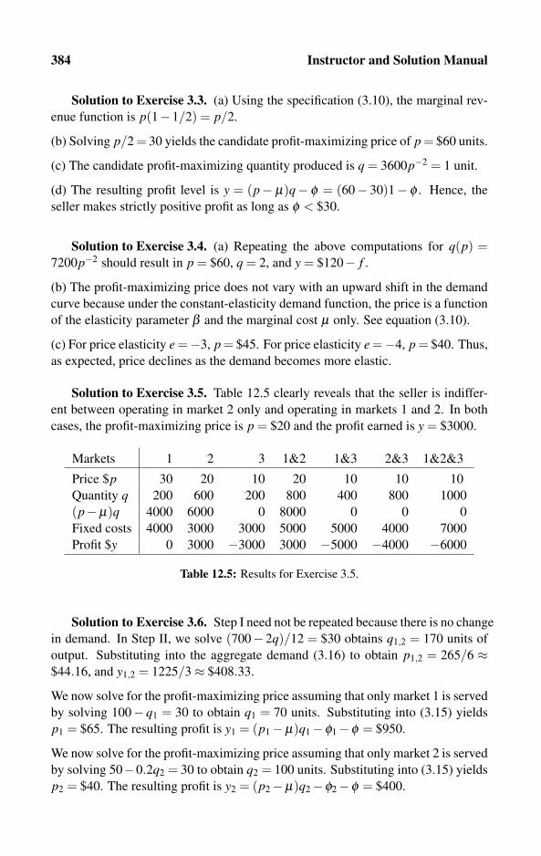
384 Instructor and Solution Manual
Solution to Exercise 3.3. (a) Using the specification (3.10), the marginal rev-
enue function is p(1−1/2) = p/2.
(b) Solving p/2 = 30 yields the candidate profit-maximizing price of p = $60 units.
(c) The candidate profit-maximizing quantity produced is q = 3600p−2 = 1 unit.
(d) The resulting profit level is y = (p− μ)q− φ = (60− 30)1− φ . Hence, the
seller makes strictly positive profit as long as φ < $30.
Solution to Exercise 3.4. (a) Repeating the above computations for q(p) =7200p−2 should result in p = $60, q = 2, and y = $120− f .
(b) The profit-maximizing price does not vary with an upward shift in the demand
curve because under the constant-elasticity demand function, the price is a function
of the elasticity parameter β and the marginal cost μ only. See equation (3.10).
(c) For price elasticity e =−3, p = $45. For price elasticity e =−4, p = $40. Thus,
as expected, price declines as the demand becomes more elastic.
Solution to Exercise 3.5. Table 12.5 clearly reveals that the seller is indiffer-
ent between operating in market 2 only and operating in markets 1 and 2. In both
cases, the profit-maximizing price is p = $20 and the profit earned is y = $3000.
Markets 1 2 3 1&2 1&3 2&3 1&2&3
Price $p 30 20 10 20 10 10 10
Quantity q 200 600 200 800 400 800 1000
(p−μ)q 4000 6000 0 8000 0 0 0
Fixed costs 4000 3000 3000 5000 5000 4000 7000
Profit $y 0 3000 −3000 3000 −5000 −4000 −6000
Table 12.5: Results for Exercise 3.5.
Solution to Exercise 3.6. Step I need not be repeated because there is no change
in demand. In Step II, we solve (700− 2q)/12 = $30 obtains q1,2 = 170 units of
output. Substituting into the aggregate demand (3.16) to obtain p1,2 = 265/6 ≈$44.16, and y1,2 = 1225/3≈ $408.33.
We now solve for the profit-maximizing price assuming that only market 1 is served
by solving 100− q1 = 30 to obtain q1 = 70 units. Substituting into (3.15) yields
p1 = $65. The resulting profit is y1 = (p1−μ)q1−φ1−φ = $950.
We now solve for the profit-maximizing price assuming that only market 2 is served
by solving 50−0.2q2 = 30 to obtain q2 = 100 units. Substituting into (3.15) yields
p2 = $40. The resulting profit is y2 = (p2−μ)q2−φ2−φ = $400.
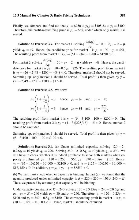
12.3 Manual for Chapter 3: Basic Pricing Techniques 385
Finally, we compare and find out that y1 = $950 > y1,2 = $408.33 > y2 = $400.
Therefore, the profit-maximizing price is p1 = $65, under which only market 1 is
served.
Solution to Exercise 3.7. For market 1, solvingdx(q1)
dq1= 100−2q1 = 2 = μ
yields q1 = 49. Hence, the candidate price for market 1 is p1 = 100− q1 = $51.
The resulting profit from market 1 is y1 = (51−2)49−1200 = $1201 > 0.
For market 2, solvingdx(q2)
dq2= 50−q2 = 2 = μ yields q2 = 48. Hence, the candi-
date price for market 2 is p2 = 50−0.5q2 = $26. The resulting profit from market 2
is y2 = (26−2)48−1200 =−$48 < 0. Therefore, market 2 should not be served.
Summing up, only market 1 should be served. Total profit is then given by y =(51−2)49−1200−1200 = $1 > 0.
Solution to Exercise 3.8. We solve
p1
(1+
1
−2
)= 3, hence p1 = $6 and q1 = 100;
p2
(1+
1
−4
)= 3, hence p2 = $4 and q2 =
225
16.
The resulting profit from market 1 is y1 = (6− 3)100− 100 = $200 > 0. The
resulting profit from market 2 is y2 = (4−3)(225/16)−15 < 0. Hence, market 2
should be excluded.
Summing up, only market 1 should be served. Total profit is then given by y =(6−3)100−100−100 = $100 > 0.
Solution to Exercise 3.9. (a) Under unlimited capacity, solving 120 − 2 ·0.25q1 = 10 yields q1 = 220. Solving 240− 2 · 0.5q2 = 10 yields q2 = 230. We
still have to check whether it is indeed profitable to serve both markets when ca-
pacity is unlimited: p1 = 120− 0.25q1 = $65, p2 = 240− 0.5q2 = $125. Hence,
y1 = (65− 10)220− 10,000 = $2100 > 0, and y2 = (125− 10)230− 10,000 =$16,450 > 0. In addition, y = y1 + y2−φ = $8550 > 0.
(b) We first must check whether capacity is binding. In part (a), we found that the
quantity produced under unlimited capacity is q = 220 + 230 = 450 > 240 = K.
Thus, we proceed by assuming that capacity will be binding.
Under capacity constraint of K = 240, solving 120−20.25q1 = 240−20.5q2 and
q1 + q2 = K = 240 yields q1 = 80 and q2 = 260. Therefore, p1 = 120−0.25q1 =$100 and p2 = 240− 0.5q2 = $160. The corresponding profit in market 1 is y1 =(100−10)80−10,000 < 0. Hence, market 1 should be excluded.

386 Instructor and Solution Manual
Assigning all the capacity to market 2 yields q2 = 240, p1 = 240−0.5240 = $120.
Hence, y2 = (120−10)240−10,000 = $16,400. Therefore, total profit is given by
y = y2−φ = $6400.
Solution to Exercise 3.10. (a) Undercutting firm 2 only is more profitable than
no undercutting if (40−δ −10)(100+200) > (20+δ −10)100, hence if δ < $20.
(b) Undercutting firms 2 and 3 is more profitable than undercutting firm 2 only if
(20− δ − 10)(100 + 200 + 300) > (40− δ − 10)(100 + 200), hence δ < −$10.
But because δ cannot be a negative number, we can conclude that undercutting
both firms is not profitable.
(c) Undercutting firms 2 and 3 is more profitable than not undercutting any firm if
(20−δ −10)(100+200+300) > (20+δ −10)100, hence if δ < 50/7≈ $7.14.
(d) Part (b) has shown that undercutting both firms yields lower profit than under-
cutting firm 2 only. Therefore, part (a) implies that firm 1 should undercut firm 2
only if δ < $20, and not undercut any firm if δ ≥ $20.
Solution to Exercise 3.11. Table 12.6 displays the computation results using
the breakeven formulas.
p1 70 60 55 40 30 20 10
q1 10 20 30 40 50 60 70
qb 2 2.5 3.33 5 10 +∞ n/a
Δq 1.11 2.86 6 13.33 50 n/a n/aΔqq1·100 1.11% 14.28% 20% 33.33% 100% n/a n/a
Table 12.6: Results for Exercise 3.11.
Solution to Exercise 3.12. (a) We solve f (120− p1)+ f (60− p2) = f (120−30− f )+ f (60−30− f ) = 550, yielding f = $5. Hence, p1 = p2 = $35. Substitut-
ing into the direct demand functions yields q1 = 120−35 = 85 and q2 = 60−35 =25. Therefore, q = q1 +q2 = 110.
(b) The breakeven constraint is now given by f1(120− 30− f1) + f (60− 30−f2) = 550, which can be solved to obtain f1 = 45−
√1475+30 f2− ( f2)2. Let us
experiment by reducing the fee in market 2 to f2 = $2. Then, f1 = 45−√1531≈$5.87. Therefore, prices are given by p1 = $35.87 and p2 = $32. Hence, the
quantities demanded are q1 = 120−35.87 ≈ 84.13 and q2 = 60−32 = 28. Thus,
total output is q = 112.13 > 110, which is the output level under a uniform fee.
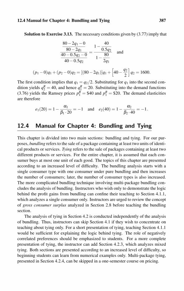
12.4 Manual for Chapter 4: Bundling and Tying 387
Solution to Exercise 3.13. The necessary conditions given by (3.77) imply that
80−2q1−0
80−2q1
40−0.5q2−0
40−0.5q2
=1− 40
0.5q2
1− 80
2q1
and
(p1−0)q1 +(p2−0)q2 = [(80−2q1)]q1 +[40− q2
2
]q2 = 1600.
The first condition implies that q1 = q2/2. Substituting for q1 into the second con-
dition yields qR2 = 40, and hence qR
1 = 20. Substituting into the demand functions
(3.76) yields the Ramsey prices pR1 = $40 and pR
1 = $20. The demand elasticities
are therefore
e1(20) = 1− α1
β1 ·20=−1 and e2(40) = 1− α2
β2 ·40=−1.
12.4 Manual for Chapter 4: Bundling and Tying
This chapter is divided into two main sections: bundling and tying. For our pur-
poses, bundling refers to the sale of a package containing at least two units of identi-
cal products or services. Tying refers to the sale of packages containing at least two
different products or services. For the entire chapter, it is assumed that each con-
sumer buys at most one unit of each good. The topics of this chapter are presented
according to an increased level of difficulty. The bundling analysis starts with a
single consumer type with one consumer under pure bundling and then increases
the number of consumers; later, the number of consumer types is also increased.
The more complicated bundling technique involving multi-package bundling con-
cludes the analysis of bundling. Instructors who wish only to demonstrate the logic
behind the profit gains from bundling can confine their teaching to Section 4.1.1,
which analyzes a single consumer only. Instructors are urged to review the concept
of gross consumer surplus analyzed in Section 2.8 before teaching the bundling
section.
The analysis of tying in Section 4.2 is conducted independently of the analysis
of bundling. Thus, instructors can skip Section 4.1 if they wish to concentrate on
teaching about tying only. For a short presentation of tying, teaching Section 4.1.1
would be sufficient for explaining the logic behind tying. The role of negatively
correlated preferences should be emphasized to students. For a more complete
presentation of tying, the instructor can add Section 4.2.3, which analyzes mixed
tying. Both sections are presented according to an increased level of difficulty, so
beginning students can learn from numerical examples only. Multi-package tying,
presented in Section 4.2.4, can be skipped in a one-semester course on pricing.
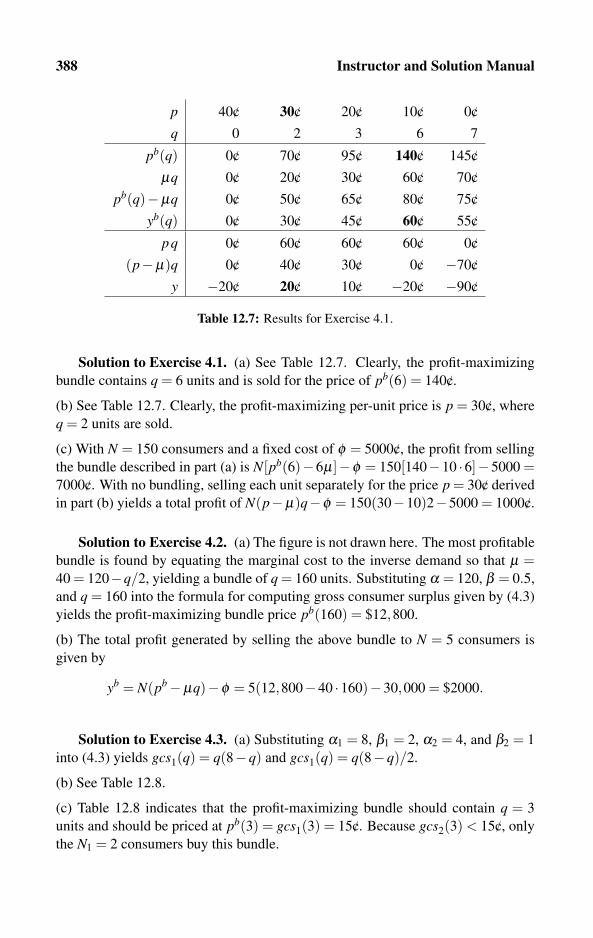
388 Instructor and Solution Manual
p 40/c 30/c 20/c 10/c 0/c
q 0 2 3 6 7
pb(q) 0/c 70/c 95/c 140/c 145/c
μq 0/c 20/c 30/c 60/c 70/c
pb(q)−μq 0/c 50/c 65/c 80/c 75/c
yb(q) 0/c 30/c 45/c 60/c 55/c
pq 0/c 60/c 60/c 60/c 0/c
(p−μ)q 0/c 40/c 30/c 0/c −70/c
y −20/c 20/c 10/c −20/c −90/c
Table 12.7: Results for Exercise 4.1.
Solution to Exercise 4.1. (a) See Table 12.7. Clearly, the profit-maximizing
bundle contains q = 6 units and is sold for the price of pb(6) = 140/c.
(b) See Table 12.7. Clearly, the profit-maximizing per-unit price is p = 30/c, where
q = 2 units are sold.
(c) With N = 150 consumers and a fixed cost of φ = 5000/c, the profit from selling
the bundle described in part (a) is N[pb(6)−6μ]−φ = 150[140−10 ·6]−5000 =7000/c. With no bundling, selling each unit separately for the price p = 30/c derived
in part (b) yields a total profit of N(p−μ)q−φ = 150(30−10)2−5000 = 1000/c.
Solution to Exercise 4.2. (a) The figure is not drawn here. The most profitable
bundle is found by equating the marginal cost to the inverse demand so that μ =40 = 120−q/2, yielding a bundle of q = 160 units. Substituting α = 120, β = 0.5,
and q = 160 into the formula for computing gross consumer surplus given by (4.3)
yields the profit-maximizing bundle price pb(160) = $12,800.
(b) The total profit generated by selling the above bundle to N = 5 consumers is
given by
yb = N(pb−μq)−φ = 5(12,800−40 ·160)−30,000 = $2000.
Solution to Exercise 4.3. (a) Substituting α1 = 8, β1 = 2, α2 = 4, and β2 = 1
into (4.3) yields gcs1(q) = q(8−q) and gcs1(q) = q(8−q)/2.
(b) See Table 12.8.
(c) Table 12.8 indicates that the profit-maximizing bundle should contain q = 3
units and should be priced at pb(3) = gcs1(3) = 15/c. Because gcs2(3) < 15/c, only
the N1 = 2 consumers buy this bundle.

12.4 Manual for Chapter 4: Bundling and Tying 389
q (Bundle Size) 1 2 3 4
gcs1(q) 7.0/c 12/c 15.0/c 16/c
y1(q) 10.0/c 16/c 18.0/c 16/c
gcs2(q) 3.5/c 6/c 7.5/c 8/c
y2(q) 9.0/c 12/c 9.0/c 0/c
min{gcs1,gcs2} 3.5/c 6/c 7.5/c 8/c
y1,2(q) 12.0/c 16/c 12.0/c 0/c
max{y1,y2,y1,2} 12.0/c 16/c 18.0/c 16/c
Table 12.8: Results for Exercise 4.3(b).
Solution to Exercise 4.4. Inspecting equation (4.14) reveals that consumer 1
will continue to prefer bundle A over bundle B, even if the price of A is raised from
pA = $13 to pA = $14. Therefore, suppose the seller offers two bundles:
Bundle 〈qA, pA〉= 〈3,$14〉: With qA = 3 units and priced at pA = $14.
Bundle 〈qB, pB〉= 〈6,$15〉: With qB = 6 units and priced at pB = $15.
Then, the market is again segmented because
ncs1(3,$14) = $15−$14 ≥ $16−$15 = ncs1(6,$15)and
ncs2(6,$15) = $15−$15 ≥ $9.75−$13 = ncs2(3,$13).
The profits from a type 1 and a type 2 consumer (not including fixed costs) are
y1 = pbA−3μ = 14−3 ·2 = $8 and y2 = pb
B−6μ = 15−6 ·2 = $3. With N1 = N2 = 1
consumer of each type, total profit is given by
yb (〈3,$14〉,〈6,$15〉) = y1 + y2−φ = $11−φ > $10−φ .
Solution to Exercise 4.5. (a) With no tying, pricing R at a high rate so that
only type 1 guests book a room, pR = $100 yields a profit of yR = (100−40)200 =$12,000. Reducing the price so that both types book a room, pR = $60 yields
a profit of yR = (60− 40)1000 = $20,000. Therefore, pR = $60 is the profit-
maximizing rate.
Setting a high breakfast price so that only type 2 consumers buy breakfast, pB =$10, yields a profit of yB = (10−2)800 = $6400. Reducing the price so that both
types buy, pB = $5, yields a profit of yB = (5−2)1000 = $3000. Therefore, pB =$10 is the profit-maximizing breakfast price.
Adding the profit made from selling these two services separately yields a profit of
yNT = 20,000+6400 = $26,400.
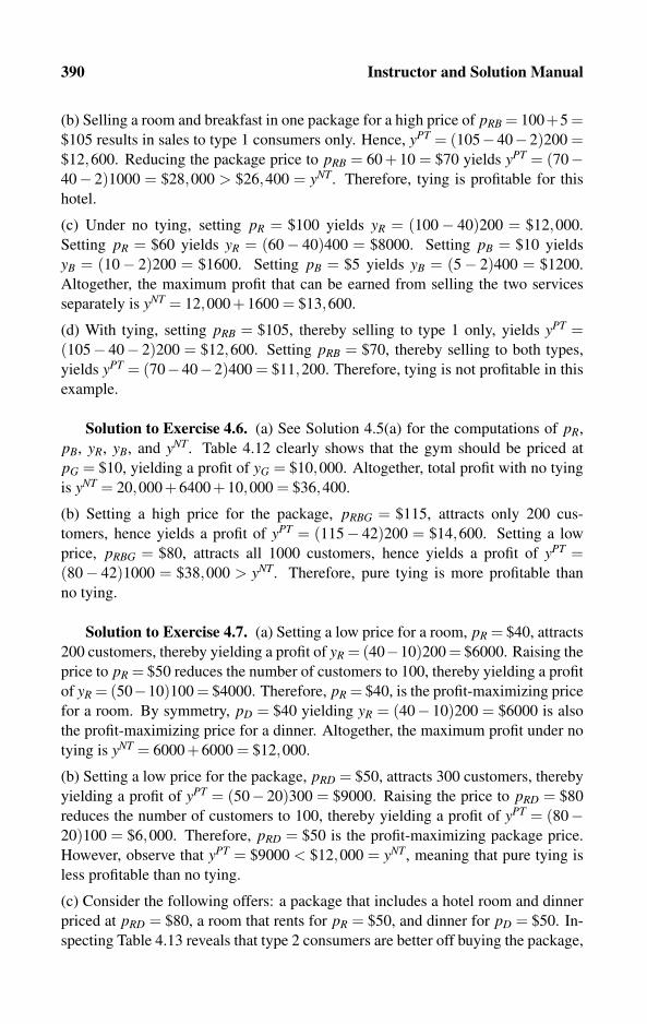
390 Instructor and Solution Manual
(b) Selling a room and breakfast in one package for a high price of pRB = 100+5 =$105 results in sales to type 1 consumers only. Hence, yPT = (105−40−2)200 =$12,600. Reducing the package price to pRB = 60 + 10 = $70 yields yPT = (70−40− 2)1000 = $28,000 > $26,400 = yNT. Therefore, tying is profitable for this
hotel.
(c) Under no tying, setting pR = $100 yields yR = (100− 40)200 = $12,000.
Setting pR = $60 yields yR = (60− 40)400 = $8000. Setting pB = $10 yields
yB = (10− 2)200 = $1600. Setting pB = $5 yields yB = (5− 2)400 = $1200.
Altogether, the maximum profit that can be earned from selling the two services
separately is yNT = 12,000+1600 = $13,600.
(d) With tying, setting pRB = $105, thereby selling to type 1 only, yields yPT =(105− 40− 2)200 = $12,600. Setting pRB = $70, thereby selling to both types,
yields yPT = (70−40−2)400 = $11,200. Therefore, tying is not profitable in this
example.
Solution to Exercise 4.6. (a) See Solution 4.5(a) for the computations of pR,
pB, yR, yB, and yNT. Table 4.12 clearly shows that the gym should be priced at
pG = $10, yielding a profit of yG = $10,000. Altogether, total profit with no tying
is yNT = 20,000+6400+10,000 = $36,400.
(b) Setting a high price for the package, pRBG = $115, attracts only 200 cus-
tomers, hence yields a profit of yPT = (115− 42)200 = $14,600. Setting a low
price, pRBG = $80, attracts all 1000 customers, hence yields a profit of yPT =(80− 42)1000 = $38,000 > yNT. Therefore, pure tying is more profitable than
no tying.
Solution to Exercise 4.7. (a) Setting a low price for a room, pR = $40, attracts
200 customers, thereby yielding a profit of yR = (40−10)200 = $6000. Raising the
price to pR = $50 reduces the number of customers to 100, thereby yielding a profit
of yR = (50−10)100 = $4000. Therefore, pR = $40, is the profit-maximizing price
for a room. By symmetry, pD = $40 yielding yR = (40− 10)200 = $6000 is also
the profit-maximizing price for a dinner. Altogether, the maximum profit under no
tying is yNT = 6000+6000 = $12,000.
(b) Setting a low price for the package, pRD = $50, attracts 300 customers, thereby
yielding a profit of yPT = (50− 20)300 = $9000. Raising the price to pRD = $80
reduces the number of customers to 100, thereby yielding a profit of yPT = (80−20)100 = $6,000. Therefore, pRD = $50 is the profit-maximizing package price.
However, observe that yPT = $9000 < $12,000 = yNT, meaning that pure tying is
less profitable than no tying.
(c) Consider the following offers: a package that includes a hotel room and dinner
priced at pRD = $80, a room that rents for pR = $50, and dinner for pD = $50. In-
specting Table 4.13 reveals that type 2 consumers are better off buying the package,
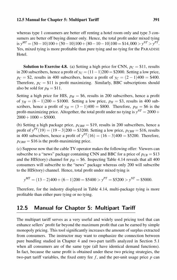
12.5 Manual for Chapter 5: Multipart Tariff 391
whereas type 1 consumers are better off renting a hotel room only and type 3 con-
sumers are better off buying dinner only. Hence, the total profit under mixed tying
is yMT = (50−10)100+(50−10)100+(80−10−10)100 = $14,000 > yNT > yPT.Yes, mixed tying is more profitable than pure tying and no tying for the PARADISE
Hotel.
Solution to Exercise 4.8. (a) Setting a high price for CNN, pC = $11, results
in 200 subscribers, hence a profit of yC = (11−1)200 = $2000. Setting a low price,
pC = $2, results in 400 subscribers, hence a profit of yC = (2− 1)400 = $400.
Therefore, pC = $11 is profit maximizing. Similarly, BBC subscriptions should
also be sold for pB = $11.
Setting a high price for HIS, pH = $6, results in 200 subscribers, hence a profit
of yH = (6− 1)200 = $1000. Setting a low price, pH = $3, results in 400 sub-
scribers, hence a profit of yH = (3− 1)400 = $800. Therefore, pH = $6 is the
profit-maximizing price. Altogether, the total profit under no tying is yNT = 2000+2000+1000 = $5000.
(b) Setting a high package price, pCBH = $19, results in 200 subscribers, hence a
profit of yPT(19) = (19−3)200 = $3200. Setting a low price, pCBH = $16, results
in 400 subscribers, hence a profit of yPT(16) = (16− 3)400 = $5200. Therefore,
pCBH = $16 is the profit-maximizing price.
(c) Suppose now that the cable TV operator makes the following offer: Viewers can
subscribe to a “news” package containing CNN and BBC for a price of pCB = $13
and the HIS(tory) channel for pH = $6. Inspecting Table 4.14 reveals that all 400
consumers will subscribe to the “news” package whereas only 200 will subscribe
to the HIS(tory) channel. Hence, total profit under mixed tying is
yMT = (13−2)400+(6−1)200 = $5400 > yPT = $5200 > yNT = $5000.
Therefore, for the industry displayed in Table 4.14, multi-package tying is more
profitable than either pure tying or no tying.
12.5 Manual for Chapter 5: Multipart Tariff
The multipart tariff serves as a very useful and widely used pricing tool that can
enhance sellers’ profit far beyond the maximum profit that can be earned by simple
monopoly pricing. This tool significantly increases the amount of surplus extracted
from consumers. The instructor may want to emphasize the connection between
pure bundling studied in Chapter 4 and two-part tariffs analyzed in Section 5.1
when all consumers are of the same type (all have identical demand functions).
In fact, because the same profit is obtained under these two pricing strategies, the
two-part tariff variables, the fixed entry fee f , and the per-unit usage price p can
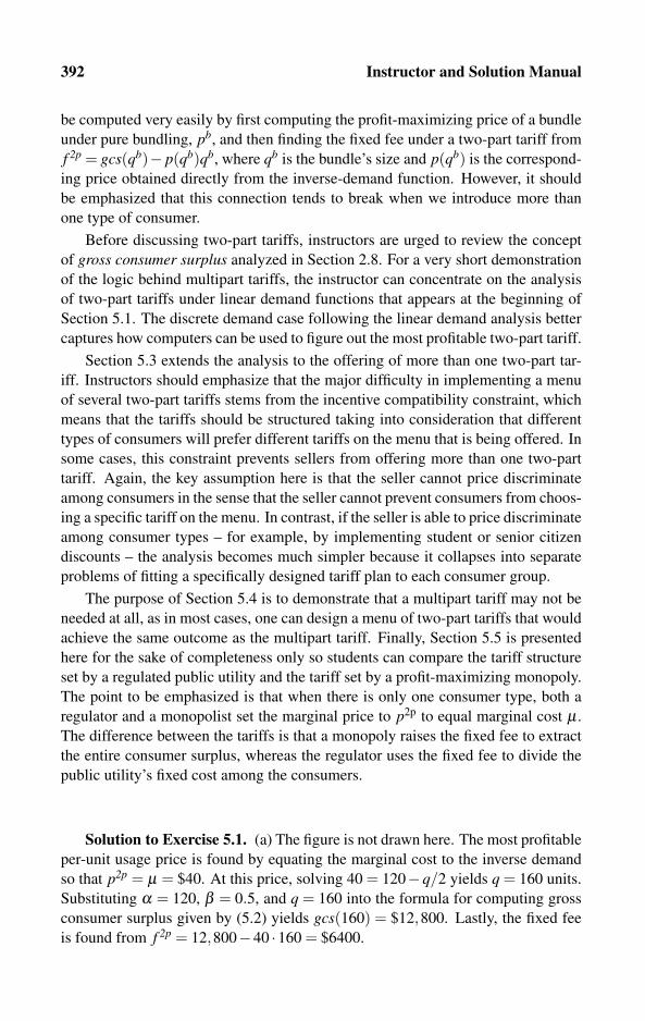
392 Instructor and Solution Manual
be computed very easily by first computing the profit-maximizing price of a bundle
under pure bundling, pb, and then finding the fixed fee under a two-part tariff from
f 2p = gcs(qb)− p(qb)qb, where qb is the bundle’s size and p(qb) is the correspond-
ing price obtained directly from the inverse-demand function. However, it should
be emphasized that this connection tends to break when we introduce more than
one type of consumer.
Before discussing two-part tariffs, instructors are urged to review the concept
of gross consumer surplus analyzed in Section 2.8. For a very short demonstration
of the logic behind multipart tariffs, the instructor can concentrate on the analysis
of two-part tariffs under linear demand functions that appears at the beginning of
Section 5.1. The discrete demand case following the linear demand analysis better
captures how computers can be used to figure out the most profitable two-part tariff.
Section 5.3 extends the analysis to the offering of more than one two-part tar-
iff. Instructors should emphasize that the major difficulty in implementing a menu
of several two-part tariffs stems from the incentive compatibility constraint, which
means that the tariffs should be structured taking into consideration that different
types of consumers will prefer different tariffs on the menu that is being offered. In
some cases, this constraint prevents sellers from offering more than one two-part
tariff. Again, the key assumption here is that the seller cannot price discriminate
among consumers in the sense that the seller cannot prevent consumers from choos-
ing a specific tariff on the menu. In contrast, if the seller is able to price discriminate
among consumer types – for example, by implementing student or senior citizen
discounts – the analysis becomes much simpler because it collapses into separate
problems of fitting a specifically designed tariff plan to each consumer group.
The purpose of Section 5.4 is to demonstrate that a multipart tariff may not be
needed at all, as in most cases, one can design a menu of two-part tariffs that would
achieve the same outcome as the multipart tariff. Finally, Section 5.5 is presented
here for the sake of completeness only so students can compare the tariff structure
set by a regulated public utility and the tariff set by a profit-maximizing monopoly.
The point to be emphasized is that when there is only one consumer type, both a
regulator and a monopolist set the marginal price to p2p to equal marginal cost μ .
The difference between the tariffs is that a monopoly raises the fixed fee to extract
the entire consumer surplus, whereas the regulator uses the fixed fee to divide the
public utility’s fixed cost among the consumers.
Solution to Exercise 5.1. (a) The figure is not drawn here. The most profitable
per-unit usage price is found by equating the marginal cost to the inverse demand
so that p2p = μ = $40. At this price, solving 40 = 120−q/2 yields q = 160 units.
Substituting α = 120, β = 0.5, and q = 160 into the formula for computing gross
consumer surplus given by (5.2) yields gcs(160) = $12,800. Lastly, the fixed fee
is found from f 2p = 12,800−40 ·160 = $6400.

12.5 Manual for Chapter 5: Multipart Tariff 393
(b) The total profit generated by selling the above bundle to N = 5 consumers is
given by
y2p = N[ f +(p−μ)q]−φ = 5[6400− (40−40)160]−30,000 = $2000.
Solution to Exercise 5.2. See Table 12.9. Clearly, the profit-maximizing two-
part tariff is f 2p = 80/c and p2p = 10/c. The consumer buys q = 6 units.
p 40/c 30/c 20/c 10/c 0/c
q 0 2 3 6 7
gcs(q) 0/c 70/c 95/c 140/c 145/c
pq 0/c 60/c 60/c 60/c 0/c
f = gcs(q)− pq 0/c 10/c 35/c 80/c 145/c
μq 0/c 20/c 30/c 60/c 70/c
y2p(q) 0/c 30/c 45/c 60/c 55/c
Table 12.9: Results for Exercise 5.2.
Solution to Exercise 5.3. (a) See Table 12.10.
p $0 $1 $2
q1 0.50 0.25 0
gcs1(q) $0.50 $0.38 $0
f1 $0.50 $0.13 $0
y1( f1, p) $0.50 $0.38 $0
q2 2.00 0.00 0
gcs2(q) $1.00 $0.00 $0
f2 $1.00 $0.00 $0
y2( f2, p) $1.00 $0.00 $0
min{ f1, f2} $0.50 $0.00 $0
y1,2(q) $1.00 $0.25 $0
max{y1,y2,y1,2} $1.00 $0.38 $0
Table 12.10: Results for Exercise 5.3.
(b) Table 12.10 clearly indicates that the maximum obtainable profit is $1.00 when
the usage price is set to p2p = $0. If the fixed fee is set to f 2p = min{ f1, f2}= $0.50,
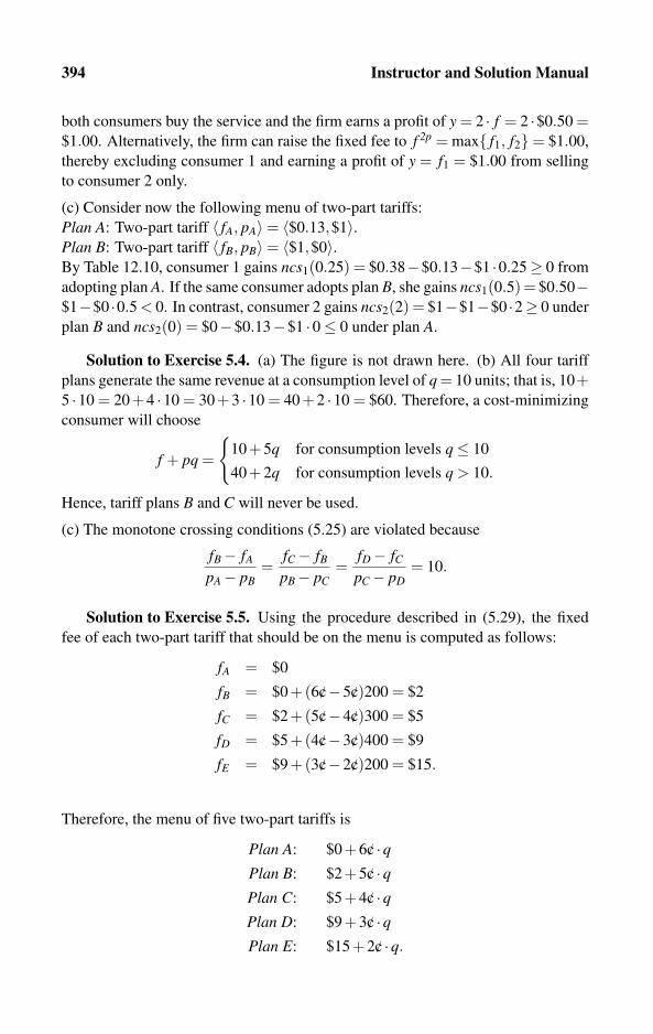
394 Instructor and Solution Manual
both consumers buy the service and the firm earns a profit of y = 2 · f = 2 ·$0.50 =$1.00. Alternatively, the firm can raise the fixed fee to f 2p = max{ f1, f2}= $1.00,
thereby excluding consumer 1 and earning a profit of y = f1 = $1.00 from selling
to consumer 2 only.
(c) Consider now the following menu of two-part tariffs:
Plan A: Two-part tariff 〈 fA, pA〉= 〈$0.13,$1〉.Plan B: Two-part tariff 〈 fB, pB〉= 〈$1,$0〉.By Table 12.10, consumer 1 gains ncs1(0.25) = $0.38−$0.13−$1 ·0.25≥ 0 from
adopting plan A. If the same consumer adopts plan B, she gains ncs1(0.5) = $0.50−$1−$0 ·0.5 < 0. In contrast, consumer 2 gains ncs2(2) = $1−$1−$0 ·2≥ 0 under
plan B and ncs2(0) = $0−$0.13−$1 ·0≤ 0 under plan A.
Solution to Exercise 5.4. (a) The figure is not drawn here. (b) All four tariff
plans generate the same revenue at a consumption level of q = 10 units; that is, 10+5 ·10 = 20+4 ·10 = 30+3 ·10 = 40+2 ·10 = $60. Therefore, a cost-minimizing
consumer will choose
f + pq =
{10+5q for consumption levels q≤ 10
40+2q for consumption levels q > 10.
Hence, tariff plans B and C will never be used.
(c) The monotone crossing conditions (5.25) are violated because
fB− fA
pA− pB=
fC− fB
pB− pC=
fD− fCpC− pD
= 10.
Solution to Exercise 5.5. Using the procedure described in (5.29), the fixed
fee of each two-part tariff that should be on the menu is computed as follows:
fA = $0
fB = $0+(6/c−5/c)200 = $2
fC = $2+(5/c−4/c)300 = $5
fD = $5+(4/c−3/c)400 = $9
fE = $9+(3/c−2/c)200 = $15.
Therefore, the menu of five two-part tariffs is
Plan A: $0+6/c ·qPlan B: $2+5/c ·qPlan C: $5+4/c ·qPlan D: $9+3/c ·qPlan E: $15+2/c ·q.

12.6 Manual for Chapter 6: Peak-load Pricing 395
12.6 Manual for Chapter 6: Peak-load Pricing
The computation of prices is based on the simple monopoly techniques of equat-
ing marginal revenue to marginal cost. Therefore, the instructor should review the
analysis of a simple monopoly facing a continuous linear demand function given in
Section 3.1.2. Furthermore, the computation of prices under the shifting-peak case
requires a vertical summation of marginal revenue functions (for the single seller
case) and of demand functions (for the regulated public utility case). The instructor
is urged to make sure that students can distinguish between vertical summation of
demand functions and the more familiar horizontal aggregation of demand func-
tions studied in Section 2.5.
The airline example given in Section 6.2.1 is sufficient for a brief introduction
to the concept of peak-load pricing. To get somewhat deeper, the instructor can
introduce the problem of a shifting peak using the example given in Section 6.3.1.
Section 6.7 on how to set peak-load prices for a regulated public utility is presented
here for the sake of completeness.
Instructors who wish to spend more time on peak-load pricing can go beyond
two seasons. The three-season example given in Section 6.5.1 is general enough
to hint at the procedure for finding which seasons should be classified has having
a shifting peak and which seasons should be classified as off-peak seasons. This
procedure is further discussed in Section 6.5.2. The instructor may want to point out
to the students that the division among the regions under which different seasons are
classified as having a shifting peak do not necessarily correspond to the kinks on the
vertical summation of the marginal revenue or demand functions. The differences
between the locations of the kinks and the dividing lines among the regions are
clearly marked in Figure 6.3 and Figure 6.5.
Section 6.6 is for more advanced students who have some experience in using
calculus. This section shows how the peak-load pricing model can be modified to
capture consumers who can delay or advance their service demand in response to
changes in the relative prices among the seasons. Before teaching this section, the
instructor should provide a brief introduction to the system of demand equations,
perhaps by going over Section 2.7, which also demonstrates how to invert a system
of demand equations.
The analysis of peak-load pricing, both for a monopoly firm and for a regulated
public utility, relies on the simple optimization procedure of equating marginal
revenue or price to the “relevant” marginal cost. However, the major difficulty is
in having to decide which type of marginal costs to apply in each season. For this
reason, the instructor should spend some time on Section 6.1, which elaborates on
how to distinguish between marginal capacity cost and marginal operating costs. In
addition, the instructor may want to discuss, at least verbally in class, the problem
of matching the lengths of time of each season with the time length under which the
marginal capacity cost μk is measured. Instructors may want to consult Section 6.8,
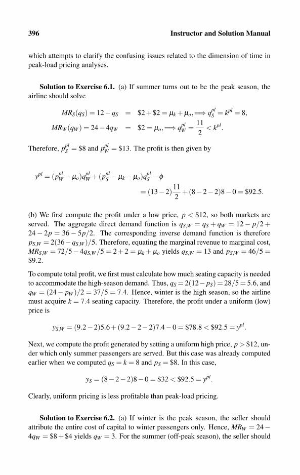
396 Instructor and Solution Manual
which attempts to clarify the confusing issues related to the dimension of time in
peak-load pricing analyses.
Solution to Exercise 6.1. (a) If summer turns out to be the peak season, the
airline should solve
MRS(qS) = 12−qS = $2+$2 = μk + μo,=⇒ qplS = kpl = 8,
MRW (qW ) = 24−4qW = $2 = μo,=⇒ qplW =
11
2< kpl.
Therefore, pplS = $8 and ppl
W = $13. The profit is then given by
ypl = (pplW −μo)q
plW +(ppl
S −μk−μo)qplS −φ
= (13−2)11
2+(8−2−2)8−0 = $92.5.
(b) We first compute the profit under a low price, p < $12, so both markets are
served. The aggregate direct demand function is qS,W = qS + qW = 12− p/2 +24− 2p = 36− 5p/2. The corresponding inverse demand function is therefore
pS,W = 2(36−qS,W )/5. Therefore, equating the marginal revenue to marginal cost,
MRS,W = 72/5−4qS,W /5 = 2 + 2 = μk + μo yields qS,W = 13 and pS,W = 46/5 =$9.2.
To compute total profit, we first must calculate how much seating capacity is needed
to accommodate the high-season demand. Thus, qS = 2(12− pS) = 28/5 = 5.6, and
qW = (24− pW )/2 = 37/5 = 7.4. Hence, winter is the high season, so the airline
must acquire k = 7.4 seating capacity. Therefore, the profit under a uniform (low)
price is
yS,W = (9.2−2)5.6+(9.2−2−2)7.4−0 = $78.8 < $92.5 = ypl.
Next, we compute the profit generated by setting a uniform high price, p > $12, un-
der which only summer passengers are served. But this case was already computed
earlier when we computed qS = k = 8 and pS = $8. In this case,
yS = (8−2−2)8−0 = $32 < $92.5 = ypl.
Clearly, uniform pricing is less profitable than peak-load pricing.
Solution to Exercise 6.2. (a) If winter is the peak season, the seller should
attribute the entire cost of capital to winter passengers only. Hence, MRW = 24−4qW = $8+$4 yields qW = 3. For the summer (off-peak season), the seller should

12.6 Manual for Chapter 6: Peak-load Pricing 397
set MRS = 12−qS = $4 (operating cost only), yielding qS = 8. Because qW < qS,
winter cannot be a peak season.
(b) If summer is the peak season, the seller should set MRS = 12−4qS = $8+$4,
yielding qS = 0. Hence, summer cannot be a peak season.
(c) Parts (a) and (b) imply a shifting-peak case. Therefore, equating vertical sum-
mation of the marginal revenue functions to the sum of marginal costs yields
∑S,W
MRv(k) = 36−5k = $8+$4+$4 =⇒ kpl = qplW = qpl
S = 4.
Substituting into the seasonal inverse demand functions yields pplW = $16 and ppl
S =$10. Total profit is therefore
ypl = (pplW −μo)kpl +(ppl
S −μo)kpl−μkkpl−φ = $40.
Solution to Exercise 6.3. (a) The marginal revenue functions are given by
MRF = 200−qF , MRW = 100−2qW ,
MRG = 100−qG, and MRS = 200−2qS.
Figure 12.4 plots all four marginal revenue functions.
(b) Vertically summing up all four marginal revenue functions obtains
∑F,W,G,S
MRv(k) =
⎧⎪⎪⎪⎪⎨⎪⎪⎪⎪⎩
600−6k if 0 < k ≤ 50
500−4k if 50 < k ≤ 100
200− k if 100 < k ≤ 200
0 if k > 200,
which is also plotted in Figure 12.4.
(c) From Figure 12.4, we can first guess (and later verify) that shifting peak oc-
curs during the fall and summer seasons only. Vertically summing up the fall and
summer marginal revenue functions and equating that sum to the sum of marginal
capacity and operating costs obtains
∑F,S
MRv(k) = 400−3k = $20+$20+$90 =⇒ kpl = 90.
Substituting the capacity level kpl = qplF = qpl
S = 90 into the fall and summer demand
functions yields pplF = $155 and ppl
S = $110.
Next, during the off-peak seasons the airline solves MRW = 100−2qW = $20 and
MRG = 100−qG = $20, yielding qplW = 40 and qpl
G = 80. At this stage, it is important

398 Instructor and Solution Manual
0 20010050
���������
���������������
MRW MRS
$300
$200
$100
��������������������������� qt , k
MRF
$400
$500
0μo = $20
$20+$20+$90
�$600!!!!!!!!!!!!��������������������������
MRG
$20+$20+$20+$20+$340
∑F,W,G,S
MRv(k)
Figure 12.4: Marginal revenue functions for Exercise 6.3.
to verify that the airline operates below capacity during the off-peak seasons by
observing that max{qplW ,qpl
G}< 90 = kpl.
Substituting into the winter and spring demand functions yields pplW = ppl
G = $60.
Finally, the total profit can be computed by
ypl = (pplF −μk−μo)kpl +(ppl
S −μo)kpl +(pplW −μo)q
plW +(ppl
G−μo)qplG−φ = $6150.
(d) Using Figure 12.4, we can first guess (and later verify) that shifting peak occurs
during all seasons. In this case, the airline solves
∑F,W,G,S
MRv(k) = 600−6k = $20+$20+$20+$20+$340 =⇒ kpl = 30.
Substituting into the four demand functions obtains pplF = $185, ppl
W = $70, pplG =
$85, and pplS = $170. Total profit is then given by
ypl = (pplF −μk−μo)kpl +(ppl
S −μo)kpl +(pplW −μo)kpl +(ppl
G−μo)kpl−φ = $2300.
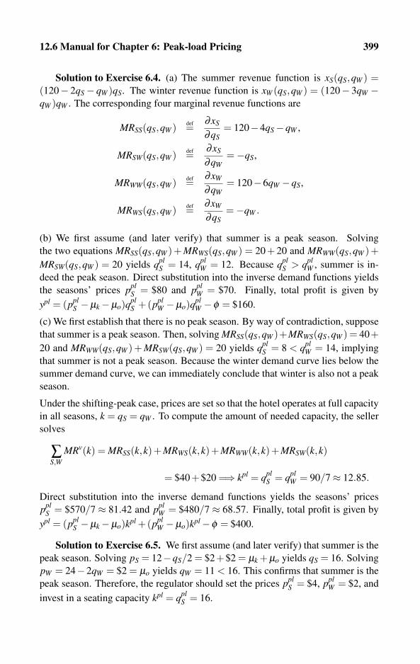
12.6 Manual for Chapter 6: Peak-load Pricing 399
Solution to Exercise 6.4. (a) The summer revenue function is xS(qS,qW ) =(120− 2qS− qW )qS. The winter revenue function is xW (qS,qW ) = (120− 3qW −qW )qW . The corresponding four marginal revenue functions are
MRSS(qS,qW ) def=∂xS
∂qS= 120−4qS−qW ,
MRSW(qS,qW ) def=∂xS
∂qW=−qS,
MRWW(qS,qW ) def=∂xW
∂qW= 120−6qW −qS,
MRWS(qS,qW ) def=∂xW
∂qS=−qW .
(b) We first assume (and later verify) that summer is a peak season. Solving
the two equations MRSS(qS,qW )+ MRWS(qS,qW ) = 20 + 20 and MRWW(qS,qW )+MRSW(qS,qW ) = 20 yields qpl
S = 14, qplW = 12. Because qpl
S > qplW , summer is in-
deed the peak season. Direct substitution into the inverse demand functions yields
the seasons’ prices pplS = $80 and ppl
W = $70. Finally, total profit is given by
ypl = (pplS −μk−μo)q
plS +(ppl
W −μo)qplW −φ = $160.
(c) We first establish that there is no peak season. By way of contradiction, suppose
that summer is a peak season. Then, solving MRSS(qS,qW )+MRWS(qS,qW ) = 40+20 and MRWW(qS,qW )+ MRSW(qS,qW ) = 20 yields qpl
S = 8 < qplW = 14, implying
that summer is not a peak season. Because the winter demand curve lies below the
summer demand curve, we can immediately conclude that winter is also not a peak
season.
Under the shifting-peak case, prices are set so that the hotel operates at full capacity
in all seasons, k = qS = qW . To compute the amount of needed capacity, the seller
solves
∑S,W
MRv(k) = MRSS(k,k)+MRWS(k,k)+MRWW(k,k)+MRSW(k,k)
= $40+$20 =⇒ kpl = qplS = qpl
W = 90/7≈ 12.85.
Direct substitution into the inverse demand functions yields the seasons’ prices
pplS = $570/7 ≈ 81.42 and ppl
W = $480/7 ≈ 68.57. Finally, total profit is given by
ypl = (pplS −μk−μo)kpl +(ppl
W −μo)kpl−φ = $400.
Solution to Exercise 6.5. We first assume (and later verify) that summer is the
peak season. Solving pS = 12−qS/2 = $2+$2 = μk + μo yields qS = 16. Solving
pW = 24−2qW = $2 = μo yields qW = 11 < 16. This confirms that summer is the
peak season. Therefore, the regulator should set the prices pplS = $4, ppl
W = $2, and
invest in a seating capacity kpl = qplS = 16.

400 Instructor and Solution Manual
Solution to Exercise 6.6. We first demonstrate that summer is not a peak sea-
son. Solving pS = 12−qS/2 = $8+$4 = μk + μo yields qS = 0. Next, we demon-
strate that winter is not a peak season by solving pW = 24− 2qW = $8 + $4 =μk + μo, yielding qW = 6. Solving pS = 12−qS/2 = $4 = μo yields qS = 16 > 6.
Therefore, a shifting-peak case prevails.
Equating the vertical sum of the demand functions to the sum of marginal costs
∑S,W
Dv(k) = 12− k2
+24−2k = 36− 5k2
= $8+$4+$4 = μk +2μo
=⇒ kpl = 8 and pplS = ppl
W = $8.
Solution to Exercise 6.7. First we demonstrate that fall is not a peak season.
If fall is a peak season, then setting pF = $20 + $100 implies that qF = 160. If
summer is an off-peak season, then setting pS = $20 implies that qS = 180 > 160,
a contradiction.
Next, we assume (and later verify) that shifting peak occurs between fall and sum-
mer, whereas winter and spring are off-peak seasons. Thus, the seller should equate
∑F,S
D(k) = 200− k2
+200− k = 400− 3k2
= $20+$20+$100
to obtain a seating capacity of kpl = 180. Substituting into the demand functions
yields pplF = $110 and ppl
S = $20.
Finally, for the off-peak periods, the seller solves pW = 100−qW = $20 and pG =100−qG/2 = $20, yielding qpl
W = 80 < kpl and qplG = 160 < kpl, which confirms that
winter and spring are off-peak seasons.
Solution to Exercise 6.8. (a) The manager should first check whether summer
is a peak season, in which case the manager should solve
120MRS(qS) = 120(240−qS) = 24,000+120 ·20,
245MRW (qW ) = 245(240−2qW ) = 245 ·20,
yielding k = qS = 20 and qW = 110. Because qW > k, summer is not a peak season.
If winter is a peak season, the manager should solve
245MRW (qW ) = 245(240−2qW ) = 24,000+120 ·20,
120MRW (qW ) = 120(240−qW ) = 120 ·20,
yielding k = qW = 2990/49 ≈ 61 and qS = 220. Because qS > k, winter is not a
peak season.

12.6 Manual for Chapter 6: Peak-load Pricing 401
Therefore, a shifting-peak season case occurs, in which case the manager should
determine the investment in room capacity according to
120MRS(k)+245MRW (k) = 120(240− k)+245(240−2k)= 24,000+365 ·20,
yielding kpl = 5630/61≈ 92.29. Therefore, the profit-maximizing prices are pplS =
240−0.5·5630/61 = 11,825/61≈ $193.85 and pplW = 240−5630/61 = 9010/61≈
$147.7 (indeed, an expensive hotel, isn’t it?).
Finally, the profit level is computed by substituting the above results into
ypl = 120(pplS −20)kpl +245(ppl
W −20)kpl−24,000k−φ
=158,484,500
61−φ ≈ $2,598,106.55−φ .
(b) The regulator should first check whether summer is a peak season, in which
case the regulator should solve
120pS(qS) = 120(240− qS
2) = 24,000+120 ·20,
245pW (qW ) = 245(240−qW ) = 245 ·20,
yielding k = qS = 40 and qW = 220. Because qW > k, summer is not a peak season.
If winter is a peak season, the regulator should solve
245pW (qW ) = 245(240−qW ) = 24,000+120 ·20,
120pS(qS) = 120(240− qS
2) = 120 ·20,
yielding k = qW = 5980/49 ≈ 122 and qS = 440. Because qS > k, winter is not a
peak season.
Therefore, a shifting-peak case occurs, in which case the regulator should deter-
mine the investment in room capacity according to
120pS(k)+245pW (k) = 120
(240− k
2
)+245(240− k)
= 24,000+365 ·20,
yielding kpl = 11,260/61≈ 184.59. Hence, the socially optimal prices are
pplS = 240−0.5
11,260
61=
9010
61≈ $147.7 and ppl
W = 240− 11,260
61=
3380
61≈ $55.4.
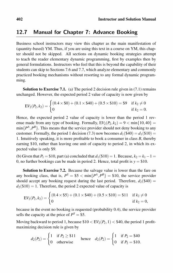
402 Instructor and Solution Manual
12.7 Manual for Chapter 7: Advance Booking
Business school instructors may view this chapter as the main manifestation of
(quantity-based) YM. Thus, if you are using this text in a course on YM, this chap-
ter should not be skipped. All sections on dynamic booking strategies attempt
to teach the reader elementary dynamic programming, first by examples then by
general formulations. Instructors who feel that this is beyond the capability of their
students can skip to Sections 7.6 and 7.7, which analyze elementary and commonly
practiced booking mechanisms without resorting to any formal dynamic program-
ming.
Solution to Exercise 7.1. (a) The period 2 decision rule given in (7.1) remains
unchanged. However, the expected period 2 value of capacity is now given by
EV2(P2,k2) =
{(0.4×$0)+(0.1×$40)+(0.5×$10) = $9 if k2 �= 0
0 if k2 = 0.
Hence, the expected period 2 value of capacity is lower than the period 1 rev-
enue made from any type of booking. Formally, EV2(P2,k2) = 9 < min{10,40}=min{PA,PB}. This means that the service provider should not deny booking to any
customer. Formally, the period 1 decision (7.3) now becomes d1($40) = d1($10) =1. Intuitively speaking, it is more profitable to book a consumer in class B, thereby
earning $10, rather than leaving one unit of capacity to period 2, in which its ex-
pected value is only $9.
(b) Given that P1 = $10, part (a) concluded that d1($10) = 1. Because, k2 = k1−1 =0, no further bookings can be made in period 2. Hence, total profit is y = $10.
Solution to Exercise 7.2. Because the salvage value is lower than the fare on
any booking class, that is, PS = $5 < min{PA,PB} = $10, the service provider
should accept any booking request during the last period. Therefore, d2($40) =d2($10) = 1. Therefore, the period 2 expected value of capacity is
EV2(P2,k2) =
{(0.4×$5)+(0.1×$40)+(0.5×$10) = $11 if k2 �= 0
0 if k2 = 0,
because in the event no booking is requested (probability 0.4), the service provider
sells the capacity at the price of PS = $5.
Moving backward to period 1, because $10 < EV2(P2,1) < $40, the period 1 profit-
maximizing decision rule is given by
d2(P2) =
{1 if P2 ≥ $11
0 otherwisehence d2(P2) =
{1 if P2 = $40
0 if P2 = $10.

12.7 Manual for Chapter 7: Advance Booking 403
Class (i): 0 A B EV2(1)Price (Pi): $0 $40 $10
π i1: 1/3 1/3 1/3
π i2 (given P1 = $0): 0 1/2 1/2
1240+ 1
210 = $25
π i2 (given P1 = $40): 1/2 0 1/2
120+ 1
210 = $5
π i2 (given P1 = $10): 1/2 1/2 0 1
20+ 1
240 = $20
Table 12.11: Computations for Exercise 7.3.
Solution to Exercise 7.3. Under three consumers, the adjusted probabilities
and expected period t = 2 values of capacity are now given by Table 12.11.
Next, the decision rule in the last booking period is clearly d2($40) = d2($10) =1 as otherwise capacity will remain unbooked. Moving backward to period t =1, the generalized decision rule given by (7.6) implies that a booking request for
class A should be accepted because P1 = $40 ≥ EV2(1)−EV2(0) = $5. Similarly,
a period t = 1 booking request for class B should be denied because P1 = $10 <EV2(1)−EV2(0) = $20. Therefore, decision rule (7.11) applies also to the present
case.
Solution to Exercise 7.4. (a) We first compute the expected value of capacity
in the last booking period, t = T :
EVT (kT ) = (0.3×$0)+(0.1×$60)+(0.6×$20) = $16,
for all kT ≥ 1. Clearly, EVT (kT ) = 0 if kT = 0.
Moving backward to period T −1, because PA > PB = 20 > 16−0, dT−1($60) =dT−1($20) = 1 (all booking requests should be accepted in period T − 1). There-
fore,
EVT−1(kT−1) = 2×16 = $32 for all kT−1 ≥ 2,
EVT−1(1) = 0.1(60+0)+0.6(20+0)+0.3×16 = $22.8.
Moving backward to booking period T − 2, dT−2($60) = dT−2($20) = 1 for all
kT−2 ≥ 3 because the amount of capacity left exceeds the number of remaining
booking periods. If kT−2 = 2, dT−2($60) = dT−2($20) = 1 because 20 > 32−22.8.
However, if kT−2 = 1, dT−2($60) = 1, whereas dT−2($20) = 0 because 20 < 22.8−0. Therefore,
EVT−2(kT−2) = 3×16 = $48 for all kT−2 ≥ 3,
EVT−2(2) = 0.1(60+22.8)+0.6(20+22.8)+0.3×32 = $43.56,
EVT−2(1) = 0.1(60+0)+0.9×22.8 = $26.52.
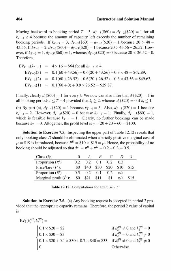
404 Instructor and Solution Manual
Moving backward to booking period T − 3, dT−3($60) = dT−2($20) = 1 for all
kT−3 ≥ 4 because the amount of capacity left exceeds the number of remaining
booking periods. If kT−3 = 3, dT−3($60) = dT−3($20) = 1 because 20 > 48−43.56. If kT−3 = 2, dT−3($60) = dT−3($20) = 1 because 20 > 43.56−26.52. How-
ever, if kT−3 = 1, dT−3($60) = 1, whereas dT−3($20) = 0 because 20 < 26.52−0.
Therefore,
EVT−3(kT−3) = 4×16 = $64 for all kT−3 ≥ 4,
EVT−3(3) = 0.1(60+43.56)+0.6(20+43.56)+0.3×48 = $62.89,
EVT−3(2) = 0.1(60+26.52)+0.6(20+26.52)+0.3×43.56 = $49.63,
EVT−3(1) = 0.1(60+0)+0.9×26.52 = $29.87.
Finally, clearly dt($60) = 1 for every t. We now can also infer that dt($20) = 1 in
all booking periods t ≤ T −4 provided that kt ≥ 2, whereas dt($20) = 0 if kt ≤ 1.
(b) By part (a), dT−4($20) = 1 because kT−4 = 3. Also, dT−3($20) = 1 because
kT−3 = 2. However, dT−2($20) = 0 because kT−2 = 1. Finally, dT−1($60) = 1,
which is feasible because kT−1 = 1. Clearly, no further bookings can be made
because kT = 0. Altogether, the profit level is y = 20+20+60 = $100.
Solution to Exercise 7.5. Inspecting the upper part of Table 12.12 reveals that
only booking class D should be eliminated when a strictly positive marginal cost of
μ = $19 is introduced, because PD = $10 < $19 = μ . Hence, the probability of no
booking should be adjusted so that π0 = π0 +πD = 0.2+0.3 = 0.5.
Class (i): 0 A B C D SProportion (π i): 0.2 0.2 0.1 0.2 0.3
Price/fare (Pi): $0 $40 $30 $20 $10 $15
Proportion (π i): 0.5 0.2 0.1 0.2 n/a
Marginal profit (Pi): $0 $21 $11 $1 n/a $15
Table 12.12: Computations for Exercise 7.5.
Solution to Exercise 7.6. (a) Any booking request is accepted in period 2 pro-
vided that the appropriate capacity remains. Therefore, the period 2 value of capital
is
EV2(kAH2 ,kHB
2 ) =⎧⎪⎪⎪⎪⎨⎪⎪⎪⎪⎩
0.1×$20 = $2 if kAH2 �= 0 and kHB
2 = 0
0.1×$30 = $3 if kAH2 = 0 and kHB
2 �= 0
0.1×$20+0.1×$30+0.7×$40 = $33 if kAH2 �= 0 and kHB
2 �= 0
0 Otherwise.
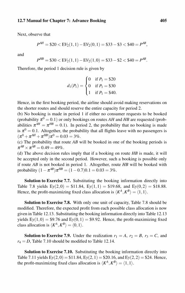
12.7 Manual for Chapter 7: Advance Booking 405
Next, observe that
PAH = $20 < EV2(1,1)−EV2(0,1) = $33−$3 < $40 = PAB,
and
PHB = $30 < EV2(1,1)−EV2(1,0) = $33−$2 < $40 = PAB.
Therefore, the period 1 decision rule is given by
d1(P1) =
⎧⎪⎨⎪⎩
0 if P1 = $20
0 if P1 = $30
1 if P1 = $40.
Hence, in the first booking period, the airline should avoid making reservations on
the shorter routes and should reserve the entire capacity for period 2.
(b) No booking is made in period 1 if either no consumer requests to be booked
(probability π0 = 0.1) or only bookings on routes AH and HB are requested (prob-
abilities πAH = πHB = 0.1). In period 2, the probability that no booking is made
is π0 = 0.1. Altogether, the probability that all flights leave with no passengers is
(π0 +πAH +πHB)π0 = 0.03 = 3%.
(c) The probability that route AB will be booked in one of the booking periods is
πAB×πAB = 0.49 = 49%.
(d) The above decision rules imply that if a booking on route HB is made, it will
be accepted only in the second period. However, such a booking is possible only
if route AB is not booked in period 1. Altogether, route HB will be booked with
probability (1−πAB)πHB = (1−0.7)0.1 = 0.03 = 3%.
Solution to Exercise 7.7. Substituting the booking information directly into
Table 7.8 yields Ey(2,0) = $11.84, Ey(1,1) = $19.68, and Ey(0,2) = $18.88.
Hence, the profit-maximizing fixed class allocation is 〈KA,KB〉= 〈1,1〉.
Solution to Exercise 7.8. With only one unit of capacity, Table 7.8 should be
modified. Therefore, the expected profit from each possible class allocation is now
given in Table 12.13. Substituting the booking information directly into Table 12.13
yields Ey(1,0) = $9.76 and Ey(0,1) = $9.92. Hence, the profit-maximizing fixed
class allocation is 〈KA,KB〉= 〈0,1〉.
Solution to Exercise 7.9. Under the realization r1 = A, r2 = B, r3 = C, and
r4 = D, Table 7.10 should be modified to Table 12.14.
Solution to Exercise 7.10. Substituting the booking information directly into
Table 7.11 yields Ey(2,0) = $11.84, Ey(2,1) = $20.16, and Ey(2,2) = $24. Hence,
the profit-maximizing fixed class allocation is 〈KA,KB〉= 〈1,1〉.

406 Instructor and Solution Manual
Booking Periods Capacity Allocation 〈KA,KB〉t = 1 t = 2 t = 3 〈1,0〉 〈0,1〉
A A A (πA)3PA 0
B A A (πA)2πBPA (πA)2πBPB
A B A (πA)2πBPA (πA)2πBPB
A A B (πA)2πBPA (πA)2πBPB
B B B 0 (πB)3PB
A B B πA(πB)2PA πA(πB)2PB
B A B πA(πB)2PA πA(πB)2PB
B B A πA(πB)2PA πA(πB)2PB
Total expected profit: Ey(1,0) Ey(0,1)
Table 12.13: Computations for Exercise 7.8.
t rt kt Booking Class (i): A B C D1 A 100 Nested allocation (Ki
1): 100 70 50 40
1 B 99 Nested allocation (Ki2): 99 70 50 40
2 C 98 Nested allocation (Ki3) : 98 69 50 40
3 D 97 Nested allocation (Ki4): 97 68 49 40
4 n/a 96 Nested allocation (Ki5): 96 67 48 39
Table 12.14: Computations for Exercise 7.9.
Solution to Exercise 7.11. With only one unit of capacity, Table 7.11 should
be modified. Therefore, the expected profit from each possible class allocation is
now given in Table 12.15. Substituting the booking information directly into Ta-
ble 12.15 yields Ey(1,0) = $9.76 and Ey(1,1) = $12. Hence, the profit-maximizing
nested class allocation is 〈1,1〉.
12.8 Manual for Chapter 8: Refund Strategies
This chapter more or less maintains an increasing level of difficulty, so the instruc-
tor should not have any problem finding which topics fit the students’ abilities best.
Proportional (percentage) refunds are analyzed only in Section 8.3.2, so instructors
who wish to skip this section as well as Section 8.2.2 can do so without any effect
on the understanding of all other sections in this chapter. Instructors teaching stu-
dents with low technical ability can focus on refund settings under an exogenously
given price, analyzed in Section 8.3. However, it may be worth a try to teach the
two consumer-type analyses presented in Section 8.4 as they give a more practical
analysis in which sellers choose price and refund levels simultaneously. Propor-

12.8 Manual for Chapter 8: Refund Strategies 407
Booking Periods Nested Allocation 〈KA,KB〉t = 1 t = 2 t = 3 〈1,0〉 〈1,1〉
A A A (πA)3PA (πA)3PA
B A A (πA)2πBPA (πA)2πBPB
A B A (πA)2πBPA (πA)2πBPA
A A B (πA)2πBPA (πA)2πBPA
B B B 0 (πB)3PB
A B B πA(πB)2PA πA(πB)2PA
B A B πA(πB)2PA πA(πB)2PB
B B A πA(πB)2PA πA(πB)2PB
Total expected profit: Ey(1,0) Ey(0,1)
Table 12.15: Computations for Exercise 7.11.
tional (percentage) refunds are ignored in some parts of this chapter. Instructors
who are short on time can simply skip all topics related to proportional refunds.
Solution to Exercise 8.1. The solution is given in Table 12.16.
π V πV p r (1−π)r U Decision
0.8 20 16 13 0 0.0 3.0 Book
0.8 20 16 14 2 0.4 2.4 No book
0.9 20 18 16 9 0.9 2.9 No book
0.2 20 4 4 3 2.4 2.4 No book
Table 12.16: Results for Exercise 8.1.
Solution to Exercise 8.2. (a) Substituting U = 3, V = 10, and π = 0.5 into
equation (8.2) yields r = 2p−4, which is drawn in Figure 12.5.
(b) Substituting r = 0 into r ≥ 2p− 4 yields p ≤ 2, which is also drawn in Fig-
ure 12.5.
(c) Substituting r = p into r ≥ 2p− 4 yields p ≤ 4, which is also drawn in Fig-
ure 12.5.
Solution to Exercise 8.3. The profit-maximizing refund level is r = 0 (no re-
fund). To prove this statement, it is sufficient to show that both types of consumers
will book the service, even under zero refund. Substituting p = 4 and Table 8.2 into
utility function (8.1) yields UL = 0.5×10⁻⁴ > 0 and UH = 0.8×10⁻⁴ > 0.

408 Instructor and Solution Manual
�r
0
���������������
r = 2p−4
r > p(ruled out)
B NB
−4
4
�
4
p2
r = p
Figure 12.5: Results for Exercise 8.2.
Solution to Exercise 8.4. (a) Under no refund, type L consumers do not book
the service because UL = 0.5×10⁻⁷ < 0. Type H consumers do book the service
because UH = 0.8× 10− 7 > 0. Substituting r = 0, p = 7, and the data from
Table 8.2 (modified to the new cost structure) into (8.4) yields the seller’s profit
level,
yNR = 500(7−3)−0.8×500×2− (1−0.8)0−1200 = 0.
(b) Both types book the service because UL = 0.5× 10− 7 +(1− 0.5)7 > 0, and
UH = 0.8×10⁻⁷+(1−0.8)7 > 0. Substituting into (8.4) yields a loss given by
yFR = (500+800)(7−3)− (0.8×500+0.5×800)×2
− (0.2×500+0.5×800)7−1200 =−1100 < 0.
(c) We compute the minimum refund level that would induce type L consumers
to book the service. Thus, we look for the minimum level of r satisfying UL =0.5× 10− 7 +(1− 0.5)r = 0, yielding a partial refund level of r = 4. Under this
refund level, the profit (8.4) is now given by
yPR = (500+800)(7−3)− (0.8×500+0.5×800)×2
− (0.2×500+0.5×800)4−1200 = 1600.
Solution to Exercise 8.5. The third and fifth columns of Table 8.3 confirm As-
sumption 8.2, thus step I of the above algorithm is now complete.
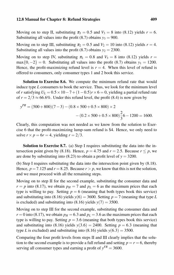
12.8 Manual for Chapter 8: Refund Strategies 409
Moving on to step II, substituting π3 = 0.5 and V3 = 8 into (8.12) yields r = 6.
Substituting all values into the profit (8.7) obtains y3 = 900.
Moving on to step III, substituting π2 = 0.5 and V2 = 10 into (8.12) yields r = 4.
Substituting all values into the profit (8.7) obtains y2 = 2300.
Moving on to step IV, substituting π1 = 0.8 and V3 = 8 into (8.12) yields r =max{0,−2} = 0. Substituting all values into the profit (8.7) obtains y1 = 1200.
Hence, the profit-maximizing refund level is r = 4. When this level of refund is
offered to consumers, only consumer types 1 and 2 book this service.
Solution to Exercise 8.6. We compute the minimum refund rate that would
induce type L consumers to book the service. Thus, we look for the minimum level
of r satisfying UL = 0.5×10⁻⁷+(1−0.5)r×6 = 0, yielding a partial refund rate
of r = 2/3≈ 66.6%. Under this refund level, the profit (8.4) is now given by
yPR = (500+800)(7−3)− (0.8×500+0.5×800)×2
− (0.2×500+0.5×800)2
36−1200 = 1600.
Clearly, this computation was not needed as we know from the solution to Exer-
cise 6 that the profit-maximizing lump-sum refund is $4. Hence, we only need to
solve r× p = 6r = 4, yielding r = 2/3.
Solution to Exercise 8.7. (a) Step I requires substituting the data into the in-
tersection point given by (8.18). Hence, p = 4.75 and r = 2.5. Because r ≤ p, we
are done by substituting into (8.23) to obtain a profit level of y = 3200.
(b) Step I requires substituting the data into the intersection point given by (8.18).
Hence, p = 7.125 and r = 8.25. Because r > p, we know that this is not the solution,
and we must proceed with all the remaining steps.
Moving on to step II for the second example, substituting the consumer data and
r = p into (8.17), we obtain pH = 7 and pL = 6 as the maximum prices that each
type is willing to pay. Setting p = 6 (meaning that both types book this service)
and substituting into (8.16) yields y(6) = 3600. Setting p = 7 (meaning that type Lis excluded) and substituting into (8.16) yields y(7) = 3500.
Moving on to step III for the second example, substituting the consumer data and
r = 0 into (8.17), we obtain pH = 6.3 and pL = 3.6 as the maximum prices that each
type is willing to pay. Setting p = 3.6 (meaning that both types book this service)
and substituting into (8.16) yields y(3.6) = 2400. Setting p = 6.3 (meaning that
type L is excluded) and substituting into (8.16) yields y(6.3) = 3500.
Comparing the four profit levels from steps II and III clearly implies that the solu-
tion to the second example is to provide a full refund and setting p = r = 6, thereby
serving all consumer types and earning a profit of yFR = 3600.
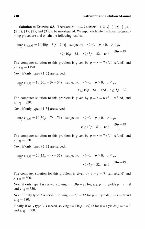
410 Instructor and Solution Manual
Solution to Exercise 8.8. There are 23−1 = 7 subsets, {1,2,3}, {1,2}, {1,3},{2,3}, {1}, {2}, and {3}, to be investigated. We input each into the linear program-
ming procedure and obtain the following results:
maxp,r
y{1,2,3} = 10[40p−3(r−34)] subject to r ≥ 0, p≥ 0, r ≤ p,
r ≥ 10p−81, r ≥ 5p−32, and10p−49
3.
The computer solution to this problem is given by p = r = 7 (full refund) and
y{1,2,3} = 1150.
Next, if only types {1,2} are served,
maxp,r
y{1,2} = 10(20p−3r−54) subject to r ≥ 0, p≥ 0, r ≤ p,
r ≥ 10p−81, and r ≥ 5p−32.
The computer solution to this problem is given by p = r = 8 (full refund) and
y{1,2} = 820.
Next, if only types {1,3} are served,
maxp,r
y{1,3} = 10(30p−7r−76) subject to r ≥ 0, p≥ 0, r ≤ p,
r ≥ 10p−81, and10p−49
3.
The computer solution to this problem is given by p = r = 7 (full refund) and
y{1,3} = 850.
Next, if only types {2,3} are served,
maxp,r
y{2,3} = 20(15p−4r−37) subject to r ≥ 0, p≥ 0, r ≤ p,
r ≥ 5p−32, and10p−49
3.
The computer solution for this problem is given by p = r = 7 (full refund) and
y{2,3} = 800.
Next, if only type 1 is served, solving r = 10p−81 for, say, p = r yields p = r = 9
and y{1} = 530.
Next, if only type 2 is served, solving r = 5p− 32 for p = r yields p = r = 8 and
y{2} = 380.
Finally, if only type 3 is served, solving r = (10p−49)/3 for p = r yields p = r = 7
and y{3} = 500.
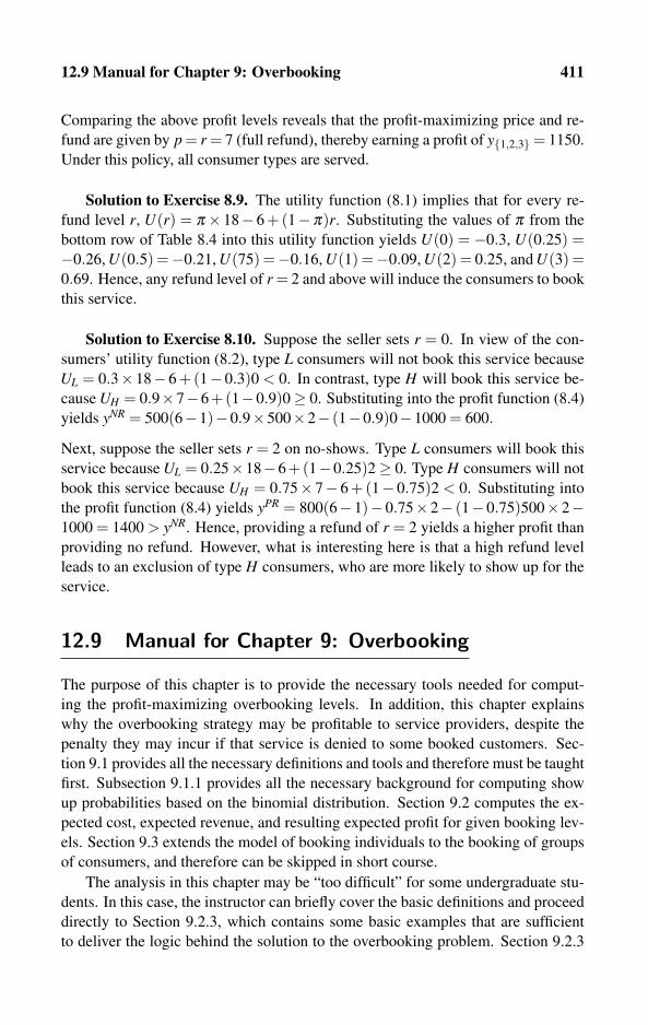
12.9 Manual for Chapter 9: Overbooking 411
Comparing the above profit levels reveals that the profit-maximizing price and re-
fund are given by p = r = 7 (full refund), thereby earning a profit of y{1,2,3}= 1150.
Under this policy, all consumer types are served.
Solution to Exercise 8.9. The utility function (8.1) implies that for every re-
fund level r, U(r) = π × 18− 6 +(1−π)r. Substituting the values of π from the
bottom row of Table 8.4 into this utility function yields U(0) = −0.3, U(0.25) =−0.26, U(0.5) =−0.21, U(75) =−0.16, U(1) =−0.09, U(2) = 0.25, and U(3) =0.69. Hence, any refund level of r = 2 and above will induce the consumers to book
this service.
Solution to Exercise 8.10. Suppose the seller sets r = 0. In view of the con-
sumers’ utility function (8.2), type L consumers will not book this service because
UL = 0.3×18−6 +(1−0.3)0 < 0. In contrast, type H will book this service be-
cause UH = 0.9×7−6+(1−0.9)0≥ 0. Substituting into the profit function (8.4)
yields yNR = 500(6−1)−0.9×500×2− (1−0.9)0−1000 = 600.
Next, suppose the seller sets r = 2 on no-shows. Type L consumers will book this
service because UL = 0.25×18−6+(1−0.25)2≥ 0. Type H consumers will not
book this service because UH = 0.75× 7− 6 +(1− 0.75)2 < 0. Substituting into
the profit function (8.4) yields yPR = 800(6−1)−0.75×2− (1−0.75)500×2−1000 = 1400 > yNR. Hence, providing a refund of r = 2 yields a higher profit than
providing no refund. However, what is interesting here is that a high refund level
leads to an exclusion of type H consumers, who are more likely to show up for the
service.
12.9 Manual for Chapter 9: Overbooking
The purpose of this chapter is to provide the necessary tools needed for comput-
ing the profit-maximizing overbooking levels. In addition, this chapter explains
why the overbooking strategy may be profitable to service providers, despite the
penalty they may incur if that service is denied to some booked customers. Sec-
tion 9.1 provides all the necessary definitions and tools and therefore must be taught
first. Subsection 9.1.1 provides all the necessary background for computing show
up probabilities based on the binomial distribution. Section 9.2 computes the ex-
pected cost, expected revenue, and resulting expected profit for given booking lev-
els. Section 9.3 extends the model of booking individuals to the booking of groups
of consumers, and therefore can be skipped in short course.
The analysis in this chapter may be “too difficult” for some undergraduate stu-
dents. In this case, the instructor can briefly cover the basic definitions and proceed
directly to Section 9.2.3, which contains some basic examples that are sufficient
to deliver the logic behind the solution to the overbooking problem. Section 9.2.3
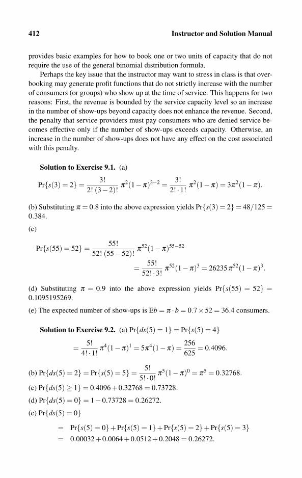
412 Instructor and Solution Manual
provides basic examples for how to book one or two units of capacity that do not
require the use of the general binomial distribution formula.
Perhaps the key issue that the instructor may want to stress in class is that over-
booking may generate profit functions that do not strictly increase with the number
of consumers (or groups) who show up at the time of service. This happens for two
reasons: First, the revenue is bounded by the service capacity level so an increase
in the number of show-ups beyond capacity does not enhance the revenue. Second,
the penalty that service providers must pay consumers who are denied service be-
comes effective only if the number of show-ups exceeds capacity. Otherwise, an
increase in the number of show-ups does not have any effect on the cost associated
with this penalty.
Solution to Exercise 9.1. (a)
Pr{s(3) = 2}=3!
2! (3−2)!π2(1−π)3−2 =
3!
2! ·1!π2(1−π) = 3π2(1−π).
(b) Substituting π = 0.8 into the above expression yields Pr{s(3) = 2}= 48/125 =0.384.
(c)
Pr{s(55) = 52}=55!
52! (55−52)!π52(1−π)55−52
=55!
52! ·3!π52(1−π)3 = 26235π52(1−π)3.
(d) Substituting π = 0.9 into the above expression yields Pr{s(55) = 52} =0.1095195269.
(e) The expected number of show-ups is Eb = π ·b = 0.7×52 = 36.4 consumers.
Solution to Exercise 9.2. (a) Pr{ds(5) = 1}= Pr{s(5) = 4}
=5!
4! ·1!π4(1−π)1 = 5π4(1−π) =
256
625= 0.4096.
(b) Pr{ds(5) = 2}= Pr{s(5) = 5}=5!
5! ·0!π5(1−π)0 = π5 = 0.32768.
(c) Pr{ds(5)≥ 1}= 0.4096+0.32768 = 0.73728.
(d) Pr{ds(5) = 0}= 1−0.73728 = 0.26272.
(e) Pr{ds(5) = 0}= Pr{s(5) = 0}+Pr{s(5) = 1}+Pr{s(5) = 2}+Pr{s(5) = 3}= 0.00032+0.0064+0.0512+0.2048 = 0.26272.
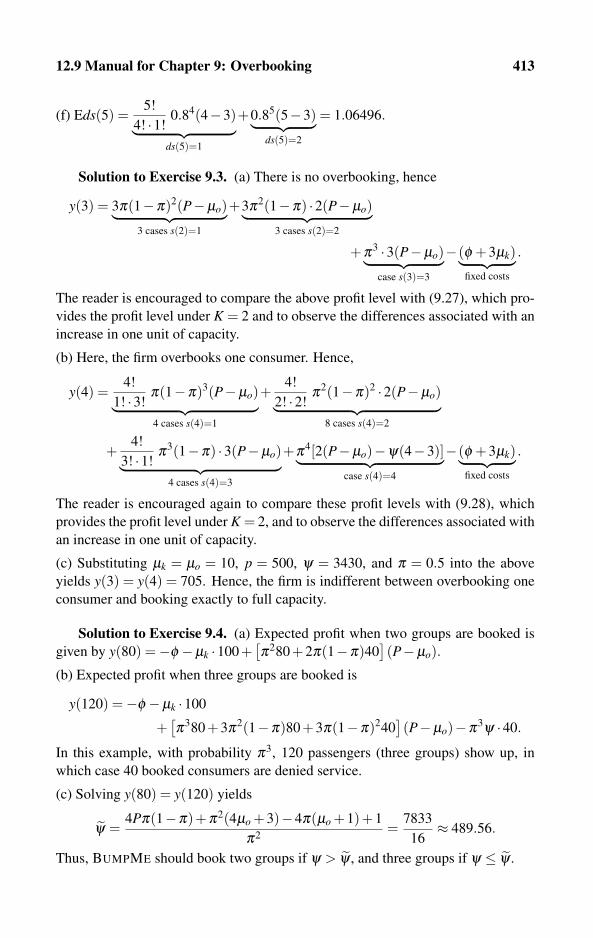
12.9 Manual for Chapter 9: Overbooking 413
(f) Eds(5) =5!
4! ·1!0.84(4−3)︸ ︷︷ ︸
ds(5)=1
+0.85(5−3)︸ ︷︷ ︸ds(5)=2
= 1.06496.
Solution to Exercise 9.3. (a) There is no overbooking, hence
y(3) = 3π(1−π)2(P−μo)︸ ︷︷ ︸3 cases s(2)=1
+3π2(1−π) ·2(P−μo)︸ ︷︷ ︸3 cases s(2)=2
+π3 ·3(P−μo)︸ ︷︷ ︸case s(3)=3
−(φ +3μk)︸ ︷︷ ︸fixed costs
.
The reader is encouraged to compare the above profit level with (9.27), which pro-
vides the profit level under K = 2 and to observe the differences associated with an
increase in one unit of capacity.
(b) Here, the firm overbooks one consumer. Hence,
y(4) =4!
1! ·3!π(1−π)3(P−μo)︸ ︷︷ ︸4 cases s(4)=1
+4!
2! ·2!π2(1−π)2 ·2(P−μo)︸ ︷︷ ︸
8 cases s(4)=2
+4!
3! ·1!π3(1−π) ·3(P−μo)︸ ︷︷ ︸
4 cases s(4)=3
+π4[2(P−μo)−ψ(4−3)]︸ ︷︷ ︸case s(4)=4
−(φ +3μk)︸ ︷︷ ︸fixed costs
.
The reader is encouraged again to compare these profit levels with (9.28), which
provides the profit level under K = 2, and to observe the differences associated with
an increase in one unit of capacity.
(c) Substituting μk = μo = 10, p = 500, ψ = 3430, and π = 0.5 into the above
yields y(3) = y(4) = 705. Hence, the firm is indifferent between overbooking one
consumer and booking exactly to full capacity.
Solution to Exercise 9.4. (a) Expected profit when two groups are booked is
given by y(80) =−φ −μk ·100+[π280+2π(1−π)40
](P−μo).
(b) Expected profit when three groups are booked is
y(120) =−φ −μk ·100
+[π380+3π2(1−π)80+3π(1−π)240
](P−μo)−π3ψ ·40.
In this example, with probability π3, 120 passengers (three groups) show up, in
which case 40 booked consumers are denied service.
(c) Solving y(80) = y(120) yields
ψ =4Pπ(1−π)+π2(4μo +3)−4π(μo +1)+1
π2=
7833
16≈ 489.56.
Thus, BUMPME should book two groups if ψ > ψ , and three groups if ψ ≤ ψ .

414 Instructor and Solution Manual
12.10 Manual for Chapter 10:
Quality, Loyalty, Auctions, and Advertising
This chapter collects some additional pricing techniques that were not included
in previous chapters. Section 10.1 ties pricing decisions to product design and
engineering decisions. It demonstrates how product design should be influenced by
the pricing technique being used and by the ability or inability to price discriminate
among the different consumer groups with respect to quality levels. This section
can be taught together with Chapter 3 (basic pricing technique); however, the major
innovation here is that the design of the product/service is endogenous, whereas in
Chapter 3, quality levels are assumed to be exogenously given.
Section 10.1 on sellers’ choice of quality and classes can be taught using the
simple examples described in Section 10.1.2. Then, the instructor can go back
to Section 10.1.1 to introduce the general notation, assumptions, and some useful
classification of consumers’ valuations. Section 10.2 on damaged goods constitutes
a natural extension of the analysis of quality given in Section 10.1. Section 10.2
can be taught at all levels as it uses numerical examples only.
Section 10.3 on pricing under competition extends the basic analysis of Sec-
tion 3.4. Section 10.3.1 analyzes price discrimination and market segmentation
based on consumers’ purchase history. This section and the exercise question uses
some calculus, which means that the section can be taught only if students have
some experience in solving optimization problems using calculus. In contrast, Sec-
tion 10.3.2 on price matching uses logical arguments only and therefore can be
taught at any level.
Section 10.4 provides a brief introduction to auctions. Instructors who wish
to devote only one lecture to auctions can concentrate on Section 10.4.1, which
analyzes open English and sealed-bid second-price auctions. The analysis of open
Dutch and sealed-bid first-price auctions given in Sections 10.4.2 and 10.4.3 are
by far more advanced than the previous sections (basically, they can be considered
graduate level).
Finally, Section 10.5, which computes the profit-maximizing expenditure on
advertising, contains one simple formula and hence can be taught at all levels.
Solution to Exercise 10.1. (a) In view of Table 10.4, the profit from selling the
fast printer is
yF =
{50(70−50) = $1000 if pF = $70
90(50−50) = $0 if pF = $50.
Next, the profit when only model M is introduced into the market is
yM =
{50(65−30) = $1750 if pM = $65
90(40−30) = $900 if pM = $40.
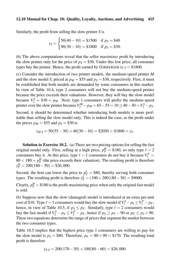
12.10 Manual for Chap. 10: Quality, Loyalty, Auctions, and Advertising 415
Similarly, the profit from selling the slow printer S is
yS =
{50(40−10) = $1500 if pS = $40
90(30−10) = $1800 if pS = $30.
(b) The above computations reveal that the seller maximizes profit by introducing
the slow printer only for the price of pS = $30. Under this low price, all consumer
types buy the printer. Hence, the profit earned by GIBBERISH is y = $1800.
(c) Consider the introduction of two printer models, the medium-speed printer Mand the slow model S, priced at pM = $55 and pS = $30, respectively. First, it must
be established that both models are demanded by some consumers in this market.
In view of Table 10.4, type 2 consumers will not buy the medium-speed printer
because the price exceeds their valuations. However, they will buy the slow model
because V S2 = $30 = pM. Next, type 1 consumers will prefer the medium-speed
printer over the slow printer because V M1 − pM = 65−55 = 10≥ 40−30 =V S
1 − pS.
Second, it should be determined whether introducing both models is more prof-
itable than selling the slow model only. This is indeed the case, as the profit under
the prices pM = $55 and pS = $30 is
yM,S = 50(55−30)+40(30−10) = $2050 > $1800 = yS.
Solution to Exercise 10.2. (a) There are two pricing options for selling the fast
original model only. First, selling at a high price, pHF = $180, so only type � = 2
consumers buy it. At this price, type � = 1 consumers do not buy it because V F1 =
80 < 180 = pHF (the price exceeds their valuation). The resulting profit is therefore
yHF = 200(180−50) = $26,000.
Second, the firm can lower the price to pLF = $80, thereby serving both consumer
types. The resulting profit is therefore yLF = (100+200)(80−50) = $9000.
Clearly, pHF = $180 is the profit-maximizing price when only the original fast model
is sold.
(b) Suppose now that the slow (damaged) model is introduced at an extra per-unit
cost of $10. Type � = 1 consumers would buy the slow model if V S1 − pS≥V F
1 − pF ,
hence, in view of Table 10.5, if pS ≤ pF . Similarly, type � = 2 consumers would
buy the fast model if V S2 − pS ≤ V F
2 − pF , hence if pS ≥ pF −90 or pF ≤ pS + 90.
These two equations determine the range of prices that segment the market between
the two consumer types.
Table 10.5 implies that the highest price type 1 consumers are willing to pay for
the slow model is pS = $80. Therefore, pF = 80 + 90 = $170. The resulting total
profit is therefore
yF,S = 200(170−50)+100(80−60) = $26,000.
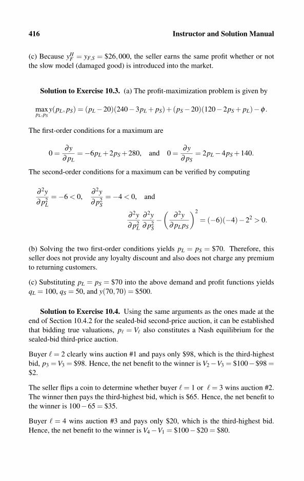
416 Instructor and Solution Manual
(c) Because yHF = yF,S = $26,000, the seller earns the same profit whether or not
the slow model (damaged good) is introduced into the market.
Solution to Exercise 10.3. (a) The profit-maximization problem is given by
maxpL,pS
y(pL, pS) = (pL−20)(240−3pL + pS)+(pS−20)(120−2pS + pL)−φ .
The first-order conditions for a maximum are
0 =∂y
∂ pL=−6pL +2pS +280, and 0 =
∂y∂ pS
= 2pL−4pS +140.
The second-order conditions for a maximum can be verified by computing
∂ 2y∂ p2
L=−6 < 0,
∂ 2y∂ p2
S=−4 < 0, and
∂ 2y∂ p2
L
∂ 2y∂ p2
S−(
∂ 2y∂ pL pS
)2
= (−6)(−4)−22 > 0.
(b) Solving the two first-order conditions yields pL = pS = $70. Therefore, this
seller does not provide any loyalty discount and also does not charge any premium
to returning customers.
(c) Substituting pL = pS = $70 into the above demand and profit functions yields
qL = 100, qS = 50, and y(70,70) = $500.
Solution to Exercise 10.4. Using the same arguments as the ones made at the
end of Section 10.4.2 for the sealed-bid second-price auction, it can be established
that bidding true valuations, p� = V� also constitutes a Nash equilibrium for the
sealed-bid third-price auction.
Buyer � = 2 clearly wins auction #1 and pays only $98, which is the third-highest
bid, p3 = V3 = $98. Hence, the net benefit to the winner is V2−V3 = $100−$98 =$2.
The seller flips a coin to determine whether buyer � = 1 or � = 3 wins auction #2.
The winner then pays the third-highest bid, which is $65. Hence, the net benefit to
the winner is 100−65 = $35.
Buyer � = 4 wins auction #3 and pays only $20, which is the third-highest bid.
Hence, the net benefit to the winner is V4−V1 = $100−$20 = $80.

12.11 Manual for Chapter 11: Tariff-choice Biases and Warranties 417
Solution to Exercise 10.5. (a) Because
ea =%Δq%Δa
= 0.05 and ep =%Δq%Δp
=−0.2,
by the Dorfman-Steiner formula (10.31), the profit-maximizing ratio of advertising
expenditure to sales revenue is given by
apq
=a
$10 million=
1
4=
0.05
−(−0.2)=
ea
−ep.
Hence, a = $2.5 million.
(b) Now, ep =−0.5. Therefore, a = 10×0.05/0.5 = $1 million.
(c) When the demand becomes more price elastic, the firm reduces the ratio of
advertising expenditure to revenue.
12.11 Manual for Chapter 11:
Tariff-choice Biases and Warranties
This last chapter introduces the student to some deviations from “rational” behavior
on the part of consumers. In other words, frequently it is observed that consumers
optimize differently from what economists expect them to do. This chapter briefly
discusses some other factors that may affect consumers’ decisions that are generally
not addressed by conventional microeconomic theory. The presentation is mostly
descriptive and therefore can be taught at any level.
The chapter ends with the analysis of the potential profit gain from supplying
warranties with the sale of products. This topic may seem to be unrelated to the
“behavioral topics” introduced earlier in this chapter; however, because warranties
also function as a psychological comforter for buyers, the students can be told that
the extra charge for including a warranty as computed in this chapter should serve
as a lower bound on how much extra a seller can actually charge for supplying a
warranty.
Solution to Exercise 11.1. Mr. Merkel ends up paying e67 for 30 rides.
Therefore, effectively, the price per ride is f /q = e67/30 = e2.33, whereas a
single ride costs only e2.10 if paid separately for each ride. Hence, by purchasing
the monthly pass, Mr. Merkel reveals that he has a flat-rate bias.
Another way of reaching the same conclusion is to realize that had Mr. Merkel
chosen the pay-per-use plan, his monthly bill would be p · q = 2.10 · 30 = e63,
which is lower than the monthly pass that costs e67.

418 Instructor and Solution Manual
Solution to Exercise 11.2. (a) The total expected gross benefit from a product
sold with a three-time replacement warranty is
πV︸︷︷︸Original purchase
+ (1−π)πV︸ ︷︷ ︸1st replacement
+ (1−π)2πV︸ ︷︷ ︸2nd replacement
+ (1−π)3πV︸ ︷︷ ︸3rd replacement
= (2−π)(π2−2π +2)πV.
The expected production cost to the seller (or the manufacturer) is
c3 = N [ μ︸︷︷︸Original
+ (1−π)μ︸ ︷︷ ︸1st replacement
+ (1−π)2μ︸ ︷︷ ︸2nd replacement
+ (1−π)3μ︸ ︷︷ ︸3rd replacement
]
= N(2−π)(π2−2π +2)μ−φ .
A monopoly seller would set the price p3 = (2−π)(π2− 2π + 2)πV . Therefore,
the total profit under a three-time replacement warranty is
y3 = N p3− c3 = N(2−π)(π2−2π +2)(πV −μ)−φ .
(b) Substituting V = $120 and μ = $60 into y3 computed in part (a) yields y3(0.9) =$53.33, y3(0.8) = $44.93, y3(0.7) = $34, y3(0.6) = $19.49, and y3(0.5) = 0. Thus,
profit increases when the product becomes more reliable (an increase in the proba-
bility π).
Solution to Exercise 11.3. (a) Expected net benefit under this “half” money-
back guarantee is
πV︸︷︷︸Expected gross benefit
− p + (1−π)p2︸ ︷︷ ︸
Refund
= πV − (1+π)p2
.
The expected cost per sale is composed of two parts: the unit production cost μ and
the expected refund (1−π)p/2. With N consumers, expected total cost is given by
chmb = N [ μ︸︷︷︸Unit cost
+ (1−π)p2︸ ︷︷ ︸
Expected refund
]−φ ,
where the subscript hmb stands for “half money-back guarantee.”
In view of the above computed net benefit function, a consumer is willing to buy
the product with this half money-back guarantee as long as
πV − (1+π)p2
≥ 0 or p≤ 2πV1+π
.
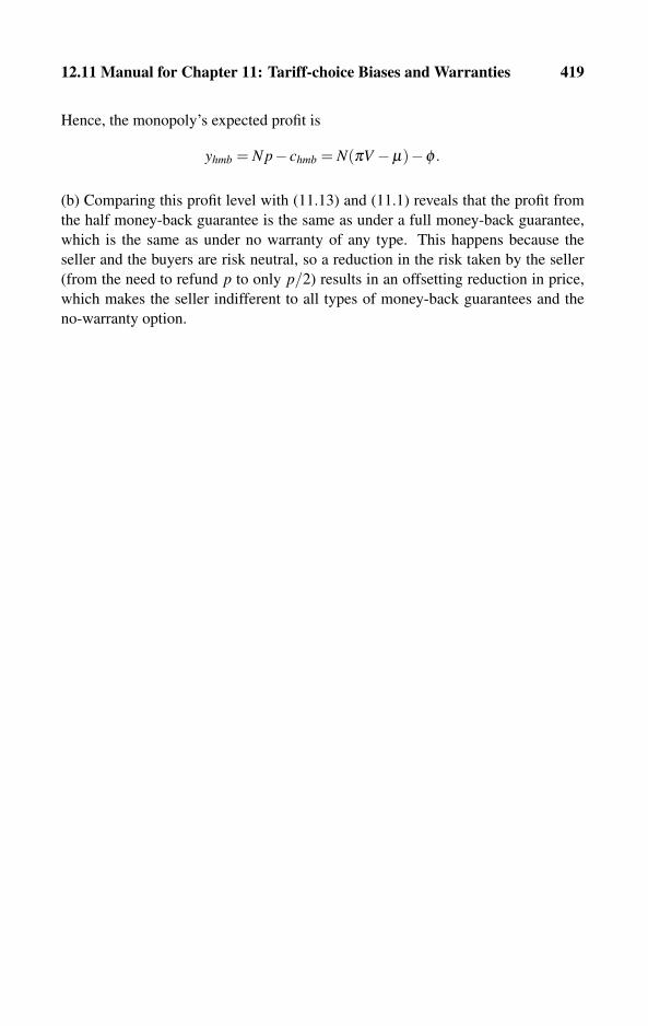
12.11 Manual for Chapter 11: Tariff-choice Biases and Warranties 419
Hence, the monopoly’s expected profit is
yhmb = N p− chmb = N(πV −μ)−φ .
(b) Comparing this profit level with (11.13) and (11.1) reveals that the profit from
the half money-back guarantee is the same as under a full money-back guarantee,
which is the same as under no warranty of any type. This happens because the
seller and the buyers are risk neutral, so a reduction in the risk taken by the seller
(from the need to refund p to only p/2) results in an offsetting reduction in price,
which makes the seller indifferent to all types of money-back guarantees and the
no-warranty option.


References
A
Adams, W., and J. Yellen. 1976. “Commodity Bundling and the Burden of Monopoly.”
Quarterly Journal of Economics 90: 475–498.
Anderson, S., and L. Leruth. 1993. “Why Firms May Prefer Not to Price Discriminate via
Mixed Bundling.” International Journal of Industrial Organization 11: 49–61.
B
Bailey, E., and L. White. 1974. “Reversals in Peak and Off-peak Prices.” Bell Journal ofEconomics 5: 75–92.
Basu, K. 1997. “Why Are So Many Goods Priced to End in Nine? And Why This Practice
Hurts the Producers.” Economics Letters 54: 41–44.
Baumol, W., and D. Bradford. 1970. “Optimal Departures from Marginal Cost Pricing.”
American Economic Review 60: 265–283.
Belobaba, P. 1987. “Airline Yield Management – An Overview of Seat Inventory Control.”
Transportation Science 21: 63–73.
Bellman, R. 1957. Applied Dynamic Programming. Princeton, N.J.: Princeton University
Press.
Belton, T. 1987. A Model of Duopoly and Meeting and Beating the Competition. Inter-national Journal of Industrial Organization 5: 399–417.
Bergstrom, T., and J. MacKie-Mason. 1991. “Some Simple Analytics of Peak-load Pric-
ing.” Rand Journal of Economics 22: 241–249.
Bodily, S., and P. Pfeifer. 1992. “Overbooking Decision Rules.” Omega 20: 129–133.
Boiteux, M. 1960. “Peak-load Pricing.” Journal of Business 33: 257–179.
Boiteux, M. 1971. “On the Management of Public Monopolies Subject to Budgetary Con-
straints.” Journal of Economic Theory 3: 219–240.
Brown, S., and D. Sibley. 1986. Public Utility Pricing. Cambridge: Cambridge University
Press.
Burstein, M. 1960. “The Economics of Tie-in Sales.” Review of Economics and Statistics42: 68–73.
422 References
CCamerer, C., G. Loewenstein, and M. Rabin. 2003. Advances in Behavioral Economics.
Princeton, N.J.: Princeton University Press.
Caminal, R., and A. Claici. 2007. “Are Loyalty-rewarding Pricing Schemes Anti-
competitive?” International Journal of Industrial Organization 25: 657–674.
Caminal, R., and C. Matutes. 1990. “Endogenous Switching Costs in a Duopoly Model.”
International Journal of Industrial Organization 8: 353–373.
Carbajo, J., D. de Meza, and D. Seidmann. 1990. “A Strategic Motivation for Commodity
Bundling.” Journal of Industrial Economics 38: 283–298.
Chen, Y. 1997a. “Equilibrium Product Bundling.” Journal of Business 70: 85–103.
Chen, Y. 1997b. “Paying Customers to Switch.” Journal of Economics & ManagementStrategy 6: 877–897.
Clay, K., D. Sibley, and P. Srinagesh. 1992. “Ex Post vs. Ex Ante Pricing: Optional
Calling Plans and Tapered Tariff.” Journal of Regulatory Economics 4: 115–138.
Coase, R. 1946. “The Marginal Cost Controversy.” Economica 13: 169–189.
Corts, K. 1995. “On the Robustness of the Argument That Price-Matching Is Anti-
competitive.” Economics Letters 47: 417–421.
Corts, K. 1997. “On the Competitive Effects of Price-matching Policies.” InternationalJournal of Industrial Organization 15: 283–299.
Courty, P. 2003. “Ticket Pricing Under Demand Uncertainty.” Journal of Law & Eco-nomics 46: 627–652.
Courty, P., and H. Li. 2000. “Sequential Screening.” Review of Economic Studies 67:
697–717.
Crew, M., C. Fernando, and P. Kleindorfer. 1995. “The Theory of Peak-load Pricing: A
Survey.” Journal of Regulatory Economics 8: 215–248.
Crew, M., and P. Kleindorfer. 1979. Public Utility Economics. New York: St. Martin’s
Press.
Crew, M., and P. Kleindorfer. 1986. The Economics of Public Utility Regulation. Cam-
bridge, Mass.: MIT Press.
DDana, J. 1998. “Advanced Purchase Discounts and Price Discrimination in Competitive
Markets.” Journal of Political Economy 106: 395–422.
Danielsen, A., D. Kamerschen, and C. Nicolaou. 1993. “Local Measured Service and the
Attributes of a Sound Rate Structure.” Journal of Economics & Finance, 17: 85–
103.
Dansby, R. 1975. “Peak Load Pricing with Time Varying Demands.” Bell Labs, Unpub-
lished.
References 423
Dansby, R., and C. Cecilia. 1984. “Commodity Bundling.” American Economic Review74: 377–381.
DellaVigna S., and U. Malmendier. 2006. “Paying Not to Go to the Gym.” AmericanEconomic Review 96: 694–719.
Demsetz, H. 1979. “Accounting for Advertising as a Barrier to Entry.” Journal of Business52: 345–360.
Deneckere, R., and P. McAfee. 1996. “Damaged Goods.” Journal of Economics and Man-agement Strategy 5: 149–174.
Dorfman, R., and P. Steiner. 1954. “Optimal Advertising and Optimal Quality.” AmericanEconomic Review 44: 826–836.
Doyle, C. 1988. “Different Selling Strategies in Bertrand Oligopoly.” Economics Letters28: 387–390.
Dreze, X., and J. Nunes. 2004. “Using Combined-currency Prices to Lower Consumers’
Perceived Cost.” Journal of Marketing Research 41: 59–72.
EEkelund, R. 1970. “Price Discrimination and Product Differentiation in Economic The-
ory: An Early Analysis.” Quarterly Journal of Economics 84: 268–278.
FFarrell J., and P. Klemperer. 2005. “Lock-in and Compatibility.” In M. Armstrong and R.
Porter (eds.), Handbook of Industrial Organization, vol. 3. Amsterdam: Elsevier.
Faulhaber, G., and J. Panzar. 1977. “Optimal Two-part Tariffs with Self-selection.” Bell
Laboratories Discussion Paper No. 74.
Feldstein, M. 1972. “Equity and Efficiency in Public Pricing.” Quarterly Journal of Eco-nomics 86: 175–187.
GGabor, A. 1955. “A Note on Block Tariffs.” Review of Economic Studies 23: 32–41.
Gabor, A. 1988. Pricing: Concepts and Methods for Effective Marketing, 2nd ed. Cam-
bridge: Gower Publishing Ltd.
Gabor, A., and W. Granger. 1966. “Price as an Indicator of Quality: Report on an En-
quiry.” Economica 33: 43–70.
Gale, I. 1993. “Price Dispersion in a Market with Advance-purchases.” Review of Indus-trial Organization 8: 451–464.
Gale, I., and T. Holmes. 1992. “The Efficiency of Advance-purchase Discounts in the
Presence of Aggregate Demand Uncertainty.” International Journal of IndustrialOrganization 10: 413–437.
424 References
Gale, I., and T. Holmes. 1993. “Advance-purchase Discounts and Monopoly Allocation
of Capacity.” American Economic Review 83: 135–146.
Gehrig, T., and R. Stenbacka. 2004. “Differentiation-induced Switching Costs and Poach-
ing.” Journal of Economics & Management Strategy 13: 635–655.
Gehrig, T., and R. Stenbacka. 2007. “Information Sharing and Lending Market Competi-
tion with Switching Costs and Poaching.” European Economic Review 51: 77–99.
Glover, F., R. Glover, J. Lorenzo, and C. McMillan. 1982. “The Passenger Mix Problem
in the Scheduled Airlines.” Interfaces 12: 73–79.
HHanson, W., and K. Martin. 1990. “Optimal Bundle Pricing.” Management Science 36:
155–174.
Hirshleifer, J. 1958. “Peak-loads and Efficient Pricing: A Comment.” Quarterly Journalof Economics 72: 451–462.
Horn, H., and O. Shy. 1996. “Bundling and International Market Segmentation.” Interna-tional Economic Review 37: 51–69.
Hviid, M., and G. Shaffer. 1999. “Hassle Costs: The Achilles’ Heel of Price-matching
Guarantees.” Journal of Economics and Management Strategy 8: 489–521.
IIngold, A., I. Yeoman, and U. McMahon. 2001. Yield Management: Strategies for the
Service Industries, 2nd ed. New York: Continuum International Publishing Group.
KKahneman, D. 2003. “Maps of Bounded Rationality: Psychology for Behavioral Eco-
nomics.” American Economic Review 93: 1449–1475.
Kaldor, N. 1950. “The Economic Aspects of Advertising.” Review of Economic Studies18: 1–27.
Kaplan, T. 2000. “Effective Price-matching: A Comment.” International Journal of In-dustrial Organization 18: 1291–1294.
Kirmani, A., and A. Rao. 2000. “No Pain, No Gain: A Critical Review of the Literature
on Signaling Unobservable Product Quality.” Journal of Marketing 64: 66–79.
Kolay, S., and G. Shaffer. 2003. “Bundling and Menus of Two-part Tariffs.” Journal ofIndustrial Economics 51: 383–403.
Kridel, D., D. Lehman, and D. Weisman. 1993. “Option Value, Telecommunications De-
mand, and Policy.” Information Economics & Policy 5: 125–144.
Krishna, V. 2002. Auction Theory. San Diego, Calif.: Academic Press.

References 425
LLaffont, J., and J. Tirole. 2001. Competition in Telecommunications. Cambridge, Mass.:
MIT Press.
Lambrecht, A., and B. Skiera. 2006. “Paying Too Much and Being Happy about It: Ex-
istence, Causes and Consequences of Tariff-choice Biases.” Journal of MarketingResearch 43: 212–223.
Lautenbacher, C., and S. Stidham. 1999. “The Underlying Markov Decision Process in the
Single-leg Airline Yield Management Problem.” Transportation Science 34: 136–
146.
Leavitt, H. 1954. “A Note on Some Experimental Findings about the Meanings of Price.”
Journal of Business 27: 205–210.
Lee, T., and M. Hersh. 1993. “A Model for Dynamic Airline Seat Inventory Control with
Multiple Seat Bookings.” Transportation Science 27: 252–265.
Lewbel, A. 1985. “Bundling of Substitutes or Complements.” International Journal ofIndustrial Organization 3: 101–107.
Liao, C., and Y. Tauman. 2002. “The Role of Bundling in Price Competition.” Interna-tional Journal of Industrial Organization 20: 365–389.
Littlechild, S. 1975. “Two-part Tariffs and Consumption Externalities.” Bell Journal ofEconomics 6: 661–670.
Littlewood, K. 1972. “Forecasting and Control of Passenger Bookings.” In Proceedingsof the Twelfth Annual AGIFORS Symposium. Nathanya, Israel.
Logan, J., and R. Lutter. 1989. “Guaranteed Lowest Prices: Do They Facilitate Collu-
sion?” Economics Letters 31: 189–192.
MMcAfee, P. 2005. Competitive Solutions: The Strategist’s Toolkit. Princeton, N.J.: Prince-
ton University Press.
McAfee, P., J. McMillan, and M. Whinston. 1989. “Multiproduct Monopoly, Commodity
Bundling, and Correlation of Values.” Quarterly Journal of Economics 114: 371–
384.
McGill, J., and G. van Ryzin. 1999. “Revenue Management: Research Overview and
Prospects.” Transportation Science 33: 233–256.
Miravete, E. 1996. “Screening Consumers through Alternative Pricing Mechanisms.” Jour-nal of Regulatory Economics 9: 111–132.
Mitchell, B. 1978. “Optimal Pricing of Local Telephone Service.” American EconomicReview 68: 517–537.
Mitchell, B., and I. Vogelsang. 1991. Telecommunication Pricing. Cambridge: Cam-
bridge University Press.
Monroe, K. 1971. “The Information Content of Prices: A Preliminary Model for Estimat-
ing Buyer Response.” Marketing Science 17: B519–B532.
426 References
Monroe, K. 2002. Pricing: Making Profitable Decisions. New York: McGraw-Hill/Irwin.
Motta, M. 2004. Competition Policy. Cambridge: Cambridge University Press.
Mullainathan, S., and R. Thaler. 2000. “Behavioral Economics.” National Bureau of Eco-
nomic Research Working Paper No. 7948.
NNagle, T., and R. Holden. 2002. The Strategy and Tactics of Pricing: A Guide to Profitable
Decision Making, 3rd ed. Upper Saddle River, N.J.: Prentice Hall.
Nalebuff, B. 2004. “Bundling as an Entry Barrier.” Quarterly Journal of Economics 119:
159–187.
Nelson, P. 1970. “Information and Consumer Behavior.” Journal of Political Economy 78:
311–329.
Nelson, P. 1974. “Advertising as Information.” Journal of Political Economy 82: 729–754.
Ng, Y., and W. Weisser. 1974. “Optimal Pricing with a Budget Constraint – The Case of
the Two-part Tariff.” Review of Economic Studies 41: 337–345.
Nunes, J. 2000. “A Cognitive Model of People’s Usage Estimations.” Journal of Market-ing Research 37: 397–426.
OOi, W. 1971. “A Disneyland Dilemma: Two-part Tariffs for a Mickey Mouse Monopoly.”
Quarterly Journal of Economics 85: 77–96.
PPhlips, L. 1988. The Economics of Imperfect Information. Cambridge: Cambridge Uni-
versity Press.
Pierce, B., and H. Winter. 1996. “Pure vs. Mixed Commodity Bundling.” Review of In-dustrial Organization 11: 811–821.
Png, I., and D. Hirshleifer. 1987. “Price Discrimination through Offers to Match Price.”
Journal of Business 60: 365–383.
RRamsey, F. 1927. “A Contribution to the Theory of Taxation.” Economic Journal 37: 47–
61.
Ringbom, S., and O. Shy. 2002. “The ‘Adjustable-curtain’ Strategy: Overbooking of Mul-
ticlass Service.” Journal of Economics 77: 73–90.
Ringbom, S., and O. Shy. 2004. “Advance Booking, Cancellations, and Partial Refunds.”
Economics Bulletin 13: 1–7.
Ringbom, S., and O. Shy. 2005. “Refunds and Collusion.” Available for downloading
from www.ozshy.com.
References 427
Rothstein, M. 1985. “O.R. and the Airline Overbooking Problem.” Operations Research33: 237–248.
SSalop, S. 1986. “Practices That (Credibly) Facilitate Oligopoly Co-ordination.” In J. Stiglitz
and F. Mathewson (eds.), New Developments in the Analysis of Market Structure.
Cambridge, Mass.: MIT Press.
Schindler, R., and P. Kirby. 1997. “Patterns of Rightmost Digits Used in Advertised
Prices: Implications for Nine-ending Effects.” Journal of Consumer Research 24:
192–201.
Schmalensee, R. 1981. “Monopolistic Two-part Pricing Arrangements.” Bell Journal ofEconomics 12: 445–466.
Schmalensee, R. 1982. “Commodity Bundling by Single-product Monopolies.” Journalof Law and Economics 25: 67–71.
Schmalensee, R. 1984. “Gaussian Demand and Community Bundling.” Journal of Busi-ness 57: S211–S230.
Seidmann, D. 1991. “Bundling as a Facilitating Device: A Reinterpretation of Leverage
Theory.” Economica 58: 491–499.
Shapiro, C., and H. Varian. 1999. Information Rules: A Strategic Guide to the NetworkEconomy. Boston: Harvard Business School Press.
Sharkey, W. 1982. The Theory of Natural Monopoly. Cambridge: Cambridge University
Press.
Sherman, R. 1989. The Regulation of Monopoly. Cambridge: Cambridge University
Press.
Shlifer, R., and Y. Vardi. 1975. “An Airline Overbooking Policy.” Transportation Science9: 101–114.
Shy, O. 1996. Industrial Organization: Theory and Applications. Cambridge, Mass.: MIT
Press.
Shy, O. 2001. The Economics of Network Industries. Cambridge: Cambridge University
Press.
Shy, O. 2002. “A Quick-and-easy Method for Estimating Switching Costs.” InternationalJournal of Industrial Organization 20: 71–87.
Shy, O., and R. Stenbacka. 2005. “Partial Outsourcing, Monitoring Cost, and Market
Structure.” Canadian Journal of Economics 38: 1173-1190.
Simon, H. 1955. “A Behavioral Model of Rational Choice.” Quarterly Journal of Eco-nomics 69: 99–118.
Simonson, I., and A. Tversky. 1992. “Choice in Context: Tradeoff Contrast, and Extreme-
ness Aversion.” Journal of Marketing Research 29: 231–295.
Steiner, P. 1957. “Peak-loads and Efficient Pricing.” Quarterly Journal of Economics 71:
585–610.
428 References
Stiving, M., and R. Winer. 1997. “An Empirical Analysis of Price Endings with Scanner
Data.” Journal of Consumer Research 24: 57–67.
TTalluri, K., and G. van Ryzin. 2004. The Theory and Practice of Revenue Management.
Boston: Kluwer Academic Publishers.
Taylor, C. 2003. “Supplier Surfing: Competition and Consumer Behavior in Subscription
Markets.” RAND Journal of Economics 34: 223–246.
Telser, L. 1964. “Advertising and Competition.” Journal of Political Economy 72: 537–
562.
Thaler, R. 1991. Quasi Rational Economics. New York: Russell Sage Foundation.
Thaler, R. 1992. The Winner’s Curse: Paradoxes and Anomalies of Economic Life. Prince-
ton, N.J.: Princeton University Press.
Thisse, J., and X. Vives. 1988. “On the Strategic Choice of Spatial Price Policy.” AmericanEconomic Review 78: 122–137.
Thomas, M., and V. Morwitz. 2005. “Penny Wise and Pound Foolish: The Left-digit
Effect in Price Cognition.” Journal of Consumer Research 32: 54–64.
Train, K., M. Ben-Akiva, and T. Atherton. 1989. “Consumption Patterns and Self-selecting
Tariffs.” Review of Economics & Statistics 71: 62–73.
Train, K., D. McFadden, and M. Ben-Akiva. 1987. “The Demand for Local Telephone
Service: A Fully Discrete Model of Residential Calling Patterns and Service Choices.”
Rand Journal of Economics 18: 109–123.
Tversky, A., and I. Simonson. 1993. “Context-dependent Preferences.” Management Sci-ence 39: 1179–1189.
VVarian, H. 1985. “Price Discrimination and Social Welfare.” American Economic Review
75: 870–875.
Varian, H. 1989. “Price Discrimination.” In R. Schmalensee and R. Willig (eds.), Hand-book of Industrial Organization. Amsterdam: North-Holland.
Varian, H. 2000. “Versioning Information Goods.” In B. Kahin and H. Varian (eds.), In-ternet Publishing and Beyond. Cambridge, Mass.: MIT Press.
Vaubourg, A. 2006. “Differentiation and Discrimination in a Duopoly with Two Bundles.”
International Journal of Industrial Organization 24: 753–762.
Venkatesh, R., and W. Kamakura. 2003. “Optimal Bundling and Pricing under a Monopoly:
Contrasting Complements and Substitutes from Independently Valued Products.”
Journal of Business 76: 211–231.
Vickrey, W. 1961. “Counterspeculation, Auctions, and Competitive Sealed Tenders.” Jour-nal of Finance 16: 8–37.
Viscusi, K., J. Vernon, and J. Harrington. 1995. Economics of Regulation and Antitrust.Cambridge, Mass.: MIT Press.
References 429
WWang, K. 1983. “Optimum Seat Allocation for Multi-leg Flights. In Proceedings of the
Twenty-Third AGIFORS Symposium. Memphis, Tenn.
Whinston, M. 1990. “Tying, Foreclosure, and Exclusion.” American Economic Review80: 837–859.
Wikipedia, the Free Encyclopedia. http://www.wikipedia.org.
Wilkie, W. 1990. Consumer Behavior, 2nd ed. New York: John Wiley & Sons.
Williamson, O. 1966. “Peak-load Pricing and Optimal Capacity under Indivisibility Con-
straints.” American Economic Review 56: 810–827.
Willig, R. 1976. “Consumer’s Surplus without Apology.” American Economic Review 66:
589–597.
Willig, R. 1978. “Pareto-superior Nonlinear Outlay Schedule.” Bell Journal of Economics9: 56–69.
Wilson, G. 1972. “The Theory of Peak-load Pricing: A Final Note.” Bell Journal of Eco-nomics and Management Science 3: 307–310.
Wilson, R. 1993. Nonlinear Pricing. Oxford: Oxford University Press.
Winer, R. 2005. Pricing. Cambridge, Mass.: Marketing Science Institute.
Wolfram, S. 2002. A New Kind of Science. Champaign, Ill.: Wolfram Media.
Wolinsky, A. 1983. “Prices as Signals of Product Quality.” Review of Economic Studies50: 647–658.

Index
Accounting, 52
Advance booking, see Booking
Advance reservation, see Booking
Adverse selection, 370
Advertising, 352
Airline industry, 11, 186, 191, 201, 250
Antitrust, 12, 13
Clayton Act, 13
per-se rule, 13
price discrimination, 13
Robinson-Patman Act, 13
rule-of-reason, 13
Arbitrage, 6, 79
Auction, 343
Backward induction, 231
Bellman’s principle, see Principle of opti-
mality
Best-response function, 97–99
Binomial distribution, see Distribution
Booking, 2
computer, 3, 246, 293
fixed class allocation, 254
group, 313
limit, 299, 319
nested class allocation, 258
network, 250
refund, 265
show-up, 299
expected, 301
Bounded rationality, 360
Breakeven, 104
formula, 99
Bumped, see Service, denied
Bundling, 7, 8, 117, 118
multiple, 129
Cable TV, 138, 142, 143
Cancellation, 266
fee, 268
probability, see Probability, survival
Capacity constraint, 10, 81, 84, 228, 299,
302
Commitment
buyer, 2
seller, 4
Complements, 43, 96
Consumer surplus, 45
gross, 46, 117, 124, 129, 154, 160, 167
marginal, 46
net, 46, 117, 129, 154, 156, 167
marginal, 46
Cost, 53
average, 53
fixed, 52, 53, 184, 269
market-specific, 67
sharing, 104
marginal, 52, 53, 231, 248
capacity, 53, 84, 184, 269, 305
operating, 53, 184, 269, 305
operating, 248
overbooking, 305
plus, 102
sunk, 52, 53, 184, 269
CRS (computer reservations system), see Book-
ing
Damaged good, 7
Decision rule, 231
Delay, see Delivery time
Delivery time, 7, 266
Demand
aggregate, 34, 74, 76
vertical, 207
correlation, 134
elastic, 23
elasticity, 23, 24, 28
arc, 25
constant, 30, 45, 51, 65, 82
cross-, 44
function, 20, 45
inelastic, 23
432 Index
inverse, 20, 23, 26
linear, 26, 50, 62, 73, 76
differentiated brands, 43, 96
network effects, 39
single-unit, 23, 34, 48, 133
Differentiation
vertical, 327
Discount, 6
quantity, 117
Distribution
binomial, 301
expected value, 301
uniform, 348
Dynamic programming, see Principle of op-
timality
Elasticity, see Demand
Equilibrium
Nash, 345, 348
Nash-Bertrand, 90, 98, 99, 341
Undercut-proof, 94
Experience goods, 353
Externality
network, 39, 40
Flow goods, 21, 214
Group
booking, 313
Hotels, 147
Hub-and-spokes network, 251
Incentive compatibility, 167
Incentive compatible, 165
Indifference curves, see Utility function
Industrial organization, 60, 89
Information goods, 22, 369
Iso-profit curves, see Profit
JavaScript, 285
Lerner’s index, 64, 66, 108
Leverage, 116
Linear programming, 285
Lock-in, 90
Loyalty, 336
Mail order, 268
Marginal cost, see Cost
Marginal revenue, see Revenue
Market segmentation, 5, 7, 8, 79, 270
bundling, 130, 167
exclusion, 68, 86
refund, 290
Money-back guarantee, 2, 374
Moral hazard
refund, 268, 291
warranties, 370
Myopic behavior, 89, 95
Network externalities, see Externality
No-show, 2, 254, 266, 298
probability, see Probability, survival
Nonlinear pricing, 115, 151
Nonprofit organization, 104
Nonstorable good, 182
Outsourcing, 55
Overbooking, 230, 297
group, 313
limit, 299
Pareto
improvement, 332
Peak-load pricing, 11, 182
shifting peak, 190
Perfect foresight, 40
Population
large, 229
small, 229
Preferences
revelation, 130, 167, 228, 343, 344
Price
matching, 340
undercutting, 91, 341
Price discrimination, 5, 12, 79
antitrust, 13
behavior-based, 336
bundling, 115
classification, 8
perfect, 119
refund, 266, 290
Principle of optimality, 231, 245, 253
Probability
defective product, 370
survival, 267, 299
average, 294
Index 433
moral hazard, 291
Profit
iso curves, 281
marginal, 101, 248
short-run, 62, 87
Public utility, see Regulated firm
Quality, 95, 326, 363, 367
damaged, 332
Ramsey prices, 108
Reaction function, see Best-response func-
tion
Refund, 2, 265, 374
lump-sum, 268
partial, 269
proportional, 268, 279
Regression, 27, 28, 31, 32
Regulated firm, 104
multipart tariff, 176
peak-load pricing, 205
Ramsey prices, 107
Resale price maintenance (RPM), 274
Reservation, see Booking
Reservation price, see Willingness to pay
Retaliation, 93, 96
Revealed preference, see Preferences
Revealed preference argument, 189, 382
Revelation, see Preferences
Revenue, 23
constant-elasticity, 33
linear demand, 29
marginal, 23, 29, 186
vertical summation, 191, 196
Revenue management, 9
RM, see Revenue management
Robinson-Patman Act, see Antitrust
Salvage value, 236, 245, 263
SCM, see Supply chain management
Scrap value, see Salvage value
Search goods, 353
Seasons, 183
Service, 2
class, 3
complementary, 228
denied, 302
expected, 304
Shifting peak, see Peak-load pricing
Shipping and handling (s&h) charges, 268
Show-up probability, see Probability, survival
Signaling, 368
Simplex method, see Linear programming
Stock goods, 21, 183
Substitutes, 43, 96
Supply chain management, 12
Survival probability, see Probability
Switching costs, 90, 336, 339, 342
Tariff
blocks, 172
multipart, 151, 171
two-part, 152
menu, 165
Telecommunication, 39
Tying, 7
mixed, 131, 142
multi-package, 131, 143
pure, 131
Undercutting, see Price
Unit elasticity, 23
Utility function, 46
iso curves, 281
refund, 271, 273
threshold, 271, 273
Value
of service/product, 4, 270
of time, 228
Volume discount, see Bundling
Warranties, 369
Welfare
consumer, 12
social, 12, 105, 106, 119, 176, 177
Willingness to pay, 4, 23, 34, 70, 95, 133,
270, 344, 370
Yield management, 9
price-based, 10
quantity-based, 10, 11
YM, see Yield management
Related Documents