Received: 18 October 2016 Revised: 30 December 2016 Accepted: 17 January 2017 Heliyon 3 (2017) e00234 Tsunami mitigation by resonant triad interaction with acoustic–gravity waves Usama Kadri a,b,∗ a School of Mathematics, Cardiff University, Cardiff, CF24 4AG, UK b Department of Mathematics, Massachusetts Institute of Technology, Cambridge, MA 02139, USA * Correspondence to: School of Mathematics, Cardiff University, Cardiff, CF24 4AG, UK. E-mail address: kadriu@cardiff.ac.uk. Abstract Tsunamis have been responsible for the loss of almost a half million lives, widespread long lasting destruction, profound environmental effects, and global financial crisis, within the last two decades. The main tsunami properties that determine the size of impact at the shoreline are its wavelength and amplitude in the ocean. Here, we show that it is in principle possible to reduce the amplitude of a tsunami, and redistribute its energy over a larger space, through forcing it to interact with resonating acoustic–gravity waves. In practice, generating the appropriate acoustic– gravity modes introduces serious challenges due to the high energy required for an effective interaction. However, if the findings are extended to realistic tsunami properties and geometries, we might be able to mitigate tsunamis and so save lives and properties. Moreover, such a mitigation technique would allow for the harnessing of the tsunami’s energy. Keywords: Applied mechanics, Acoustics 1. Introduction Tsunamis are water waves caused by the displacement of a large volume of water, in the deep ocean or a large lake, following an earthquake, landslide, underwater explosion, meteorite impacts, or other violent geological events. On the coastline, the resulting waves evolve from unnoticeable to devastating, reaching heights of tens http://dx.doi.org/10.1016/j.heliyon.2017.e00234 2405-8440/© 2017 The Author. Published by Elsevier Ltd. This is an open access article under the CC BY-NC-ND license (http://creativecommons.org/licenses/by-nc-nd/4.0/).

Welcome message from author
This document is posted to help you gain knowledge. Please leave a comment to let me know what you think about it! Share it to your friends and learn new things together.
Transcript
Received:18 October 2016
Revised:30 December 2016
Accepted:17 January 2017
Heliyon 3 (2017) e00234
http://dx.doi.org/10.1016/j.heliyon.20
2405-8440/© 2017 The Author. Publ
(http://creativecommons.org/licenses/
Tsunami mitigation by
resonant triad interaction with
acoustic–gravity wavesUsama Kadri a,b,∗
a School of Mathematics, Cardiff University, Cardiff, CF24 4AG, UKb Department of Mathematics, Massachusetts Institute of Technology, Cambridge, MA 02139, USA
* Correspondence to: School of Mathematics, Cardiff University, Cardiff, CF24 4AG, UK.
E-mail address: [email protected].
Abstract
Tsunamis have been responsible for the loss of almost a half million lives, widespread
long lasting destruction, profound environmental effects, and global financial crisis,
within the last two decades. The main tsunami properties that determine the size
of impact at the shoreline are its wavelength and amplitude in the ocean. Here,
we show that it is in principle possible to reduce the amplitude of a tsunami,
and redistribute its energy over a larger space, through forcing it to interact with
resonating acoustic–gravity waves. In practice, generating the appropriate acoustic–
gravity modes introduces serious challenges due to the high energy required for
an effective interaction. However, if the findings are extended to realistic tsunami
properties and geometries, we might be able to mitigate tsunamis and so save lives
and properties. Moreover, such a mitigation technique would allow for the harnessing
of the tsunami’s energy.
Keywords: Applied mechanics, Acoustics
1. Introduction
Tsunamis are water waves caused by the displacement of a large volume of water,
in the deep ocean or a large lake, following an earthquake, landslide, underwater
explosion, meteorite impacts, or other violent geological events. On the coastline,
the resulting waves evolve from unnoticeable to devastating, reaching heights of tens
17.e00234
ished by Elsevier Ltd. This is an open access article under the CC BY-NC-ND license by-nc-nd/4.0/).

Article No~e00234
2 http://dx.doi.org/10.1016/j.he
2405-8440/© 2017 The Author. Publ
(http://creativecommons.org/licenses/
of meters and causing destruction of property and loss of life. Over 225,000 people
were killed in the 2004 Indian Ocean tsunami alone. For many decades, scientists
have been studying tsunami, and progress has been widely reported in connection
with the causes [1], forecasting [2], and recovery [3]. However, to our knowledge,
none of the studies ratifies the approach of a direct mitigation of tsunamis, with the
exception of mitigation using submarine barriers (e.g. see Ref. [4]). In an attempt to
open a discussion on this approach, we examine the feasibility of redistributing the
total energy of a very long surface ocean (gravity) wave over a larger space through
interaction with acoustic–gravity waves.
Acoustic–gravity waves (AGWs) are sound waves that propagate in the water
layer with amplitudes governed by the restoring force of gravity. Since the slight
compressibility of the water has a negligible effect on surface gravity waves, on
one hand, and the gravitational force has no practical effect on sound waves in the
ocean, on the other hand, the compressibility and gravity effects in water have long
been treated separately. Consequently, AGWs that rely on the interplay between
acoustic and gravity wave modes have not yet received proper attention. AGWs
have typically wavelengths of tens or hundreds of kilometers, and propagate at near
the speed of sound in water (1500 m/s), at relatively low frequencies ranging from
0.1–100 Hz. Unlike surface ocean waves, AGWs form with tsunamis and induce
pressure disturbances not only near the surface but in the whole water column,
reaching the sea-floor where they leave measurable pressure signatures [5], which
makes them perfect tsunami precursors (Figure 1(a)). In fact, with only two low-
frequency bottom-pressure sensors, one can identify the epicenter location, from
arrival time delay, and the fact that the pressure decreases proportional to the inverse
square-root of the distance — or by employing the inverse solution given by Ref. [6].
Such a detection station should be installed in the deep ocean where AGWs are
expected to travel freely in the water column. This has clear benefits relative to
standard warning systems that rely on the actual arrival of the tsunami. As an
example, the 2004 Indian Ocean earthquake that occurred at 00:58 UTC generated a
tsunami that hit the coastal villages of Indonesia 14 minutes later, at 01:12 UCT, and
Sri Lanka 71 minutes later at 02:23 UCT. If an AGW based alarm system existed at
that time at a distance of a thousand kilometers from the epicenter, almost regardless
to direction, the tsunami could have been detected at 01:09 UTC, that is 3 and 60
minutes before it hit Indonesia and Sri Lanka, respectively, which could have saved
many lives (see Figure 1(a)).
Besides acting as tsunami precursors, AGWs can exchange and share energy with
surface ocean waves in a three-wave interaction mechanism known as a resonant
triad (see Refs. [7, 8]). A general theory on resonant triad interactions of AGWs was
developed recently [9]. The theory considers the interaction of two surface ocean
liyon.2017.e00234
ished by Elsevier Ltd. This is an open access article under the CC BY-NC-ND license by-nc-nd/4.0/).

Article No~e00234
3 http://dx.doi.org/10.1016/j.he
2405-8440/© 2017 The Author. Publ
(http://creativecommons.org/licenses/
Figure 1. Detection and mitigation system. (a): Schematic illustration of tsunami and acoustic–gravity waves (AGWs) generated during the 2004 Indian Ocean earthquake. The AGWs travel much faster than the tsunami reaching the proposed detection station, at a distance of 1,000 km from the epicenter, within 11 minutes; that leaves 3 and 60 minutes before the tsunami hits Indonesia and Sri Lanka, respectively. (b): Schematic illustration of the proposed mitigation system. Two AGWs are transmitted towards the tsunami, to form a resonant triad.
wave packets of similar periods but opposite directions and shows how these give
rise to an AGW of a similar frequency, but much larger wavelength. It also shows
that the interaction of wave packets is far less efficient, in terms of energy exchange,
than the interaction of a train of sinusoidal waves. While this energy exchange
provides a natural explanation of the generation of oceanic microseisms [10] —
small oscillations of the seafloor in the frequency range of 0.1–0.3 Hz — it suggests
that mitigation of surface gravity waves is possible through a careful resonant triad
interaction.
In order to utilize the suggested mitigation mechanism, we consider a more practical
interaction comprising a single long surface ocean wave, representing the tsunami,
and two AGWs. In the current settings, all triad members have a comparable
lengthscale, whilst the two AGWs have much larger timescales [11]. The wavelength
of the tsunami is assumed longer than a regular surface ocean wave, but short enough
that the dispersion relation is still observed. Once a tsunami is identified, e.g. using
the early detection warning system employed above, we transmit two finely tuned
trains of AGWs that upon interaction with the tsunami form a resonant triad, as
illustrated in Figure 1(b).
liyon.2017.e00234
ished by Elsevier Ltd. This is an open access article under the CC BY-NC-ND license by-nc-nd/4.0/).
Article No~e00234
4 http://dx.doi.org/10.1016/j.he
2405-8440/© 2017 The Author. Publ
(http://creativecommons.org/licenses/
2. Background
2.1. Governing equations
Following [10], we consider a two dimensional Cartesian coordinate system (𝑥, 𝑧)with the origin in the undisturbed free surface, and the 𝑧-axis vertically upwards;
the density is a function of pressure alone, the earth curvature and the viscosity are
neglected, and the velocity 𝐮 is assumed irrotational, so that 𝐮 = ∇𝜑. Let 𝑧 = 𝜂 be
the equation of the free surface, and 𝑧 = −ℎ the equation of the rigid flat bottom.
Approximate to quadratic terms, the equations of motion can then be integrated to
obtain the field equation [10]
𝜑𝑡𝑡 − 𝑐2∇2𝜑 + 𝑔𝜑𝑧 = −2𝜑𝑥𝜑𝑥𝑡 − 2𝜑𝑧𝜑𝑧𝑡 (−ℎ ≤ 𝑧 ≤ 0), (1)
where 𝑐 is the speed of sound in the fluid, 𝑔 is the gravitational acceleration, and 𝑡 is
the time.
The boundary condition on the rigid bottom is
𝜑𝑧 = 0 (𝑧 = −ℎ). (2)
On the free surface, the usual kinematic and dynamic conditions apply, and the
combined condition read (see Ref. [11])
𝜑𝑡𝑡 + 𝑔𝜑𝑧 = −2𝜑𝑥𝜑𝑥𝑡 − 2𝜑𝑧𝜑𝑧𝑡 + 𝑔−1𝜑𝑡𝜑𝑡𝑡𝑧 + 𝜑𝑡𝜑𝑧𝑧 (𝑧 = 0). (3)
2.2. Dispersion relation
Applying a separation of variables in the linearized field equation results in an
ordinary differential equation. The solution of the equation results in the following
AGW dispersion relation upon substitution in the boundary conditions,
𝜔2 = −𝑔𝜇 tan(𝜆ℎ), (4)
where 𝑘2 = 𝜔2∕𝑐2 − 𝜆2, with real 𝑘 and 𝜆. Note that for a small scale dispersive
tsunami of frequency 𝜔 = 𝜎, traveling on deep water, 𝜆 ≃ i𝑘 is pure imaginary and
the dispersion relation reduces to
𝜎2 = 𝑔𝑘, (5)
which is the well-known surface gravity wave dispersion relation.
liyon.2017.e00234
ished by Elsevier Ltd. This is an open access article under the CC BY-NC-ND license by-nc-nd/4.0/).

Article No~e00234
5 http://dx.doi.org/10.1016/j.he
2405-8440/© 2017 The Author. Publ
(http://creativecommons.org/licenses/
2.3. Resonant triads
In the problem at hand, the triad comprises two acoustic modes, (𝜔1, 𝑞1), (𝜔2, 𝑞2), and a tsunami (𝜎, 𝑘), that satisfy the resonance conditions
𝜎 = 𝜔1 − 𝜔2, 𝑘 = 𝑞1 + 𝑞2, (6)
and the dispersion relations (4) and (5).
Defining a potential that comprises a tsunami and two AGWs, substituting in the
governing equations, and imposing a solvability condition, results in the amplitude
evolution equations for the tsunami, and the two AGWs in the form
d𝑆d𝜏
= −𝛽𝐴∗1𝐴2, (7)
𝜕𝐴1𝜕𝜏
= −𝛾1𝜕𝐴1𝜕𝜉
+ 𝛼1𝐴2𝑆∗,
𝜕𝐴2𝜕𝜏
= −𝛾2𝜕𝐴2𝜕𝜉
− 𝛼2𝐴1𝑆, (8)
where 𝛼1, 𝛼2, 𝛾1, 𝛾2, and 𝛽 are constants defined by
𝛼1 =1
2𝑔2 cos(𝜆1ℎ)
×{(
2𝑔𝜎𝑞1 + 𝜔31 + 2𝜎2𝜔1 + 2𝜎𝜔2
1 − 𝜎3)𝜎 cos(𝜆2ℎ) + 2𝑔𝜎2𝜆2 sin(𝜆2ℎ)
}
𝛼2 =1
2𝑔2 cos(𝜆2ℎ)
{(2𝑔𝜎𝑞1 + 𝜔3
1 + 𝜎2𝜔1 + 𝜎𝜔21)𝜎 cos(𝜆1ℎ) − 2𝑔𝜎2𝜆1 sin(𝜆1ℎ)
}
𝛾1 = −𝑔𝑞1
𝜔1𝜆1 cos(𝜆1ℎ), 𝛾2 = −
𝑔𝑞2𝜔2𝜆2 cos(𝜆2ℎ)
.
3. Results
3.1. Redistribution of energy
In order to demonstrate the results effectively we consider a numerical example
whereby the depth ℎ = 3000 m, 𝑐 = 1500 m∕s, 𝑔 = 9.81 m∕s2; 𝜔1 = 1 rad∕s,
and the corresponding frequencies, 𝜎 = 0.084 rad∕s, 𝜔2 = 0.916 rad∕s; and 𝛼1 =𝛼2 = 1, 𝛽 = −1, 𝛾1 = 𝛾2 = 1. In addition, we consider the tsunami and the AGW
envelopes to be Gaussian with initial amplitudes,
𝑆0 = e−𝑥2 𝐴10 = e−𝑥2
2𝑏2 , 𝐴20 = e−𝑥2
2𝑏2 , (9)
where a standard deviation (Gaussian widths) 𝑏 = 2−1∕2 was considered in the main
example. As the interaction proceeds, energy is withdrawn from the tsunami to the
AGWs, which due to their high propagation speed transfer the withdrawn energy
away from the original tsunami envelope. Thus, the total energy of the tsunami
liyon.2017.e00234
ished by Elsevier Ltd. This is an open access article under the CC BY-NC-ND license by-nc-nd/4.0/).

Article No~e00234
6 http://dx.doi.org/10.1016/j.he
2405-8440/© 2017 The Author. Publ
(http://creativecommons.org/licenses/
Figure 2. Evolution of amplitudes. As the tsunami propagates from right to left it interacts with two transmitted trains of acoustic–gravity waves, that propagate from left to right. After the interaction, the tsunami envelope is redistributed behind over a larger space and its amplitude is reduced.
is redistributed over a larger area, and the initial tsunami amplitude is reduced
(Figure 2). Consequently, as the tsunami approaches the shoreline, its run-up height
decreases accordingly and the impact at the shoreline reduces. In theory, the tsunami
energy redistribution process by AGWs can be repeated over and over until the
tsunami is completely dispersed, and the run-up height is minimal. However, this
may require a very long interaction time in particular for lower frequencies.
3.2. Energy estimation
To evaluate the amount of energy within the AGW modes we consider the case
without a spatial dependency, whereby an analytical solution in the form of Jacobi
elliptic functions can be formulated [11]
|𝑆|2 = |𝑆0|2 − 𝛽
𝛼1|𝐴10|2sn2(𝑢, 𝜃) (10)
|𝐴1|2 = |𝐴10|2cn2(𝑢, 𝜃), |𝐴2|2 = 𝛼2𝛼
|𝐴10|2sn2(𝑢, 𝜃) (11)
1liyon.2017.e00234
ished by Elsevier Ltd. This is an open access article under the CC BY-NC-ND license by-nc-nd/4.0/).
Article No~e00234
7 http://dx.doi.org/10.1016/j.he
2405-8440/© 2017 The Author. Publ
(http://creativecommons.org/licenses/
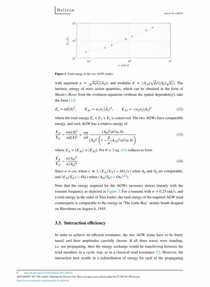
Figure 3. Total energy in the two AGW modes.
with argument 𝑢 =√𝛼1𝛼2|𝑆0|𝜏 and modulus 𝜃 = |𝐴10|√𝛽∕(|𝑆0|√𝛼1). The
intrinsic energy of wave action quantities, which can be obtained in the form of
Manley–Rowe from the evolution equations (without the spatial dependency), take
the form [11]
𝐸𝑠 = 𝜎𝛽|𝑆|2, 𝐸𝐴1 = 𝜔1𝛼1|𝐴1|2, 𝐸𝐴2 = −𝜔2𝛼2|𝐴2|2 (12)
where the total energy 𝐸𝑠+𝐸1 +𝐸2 is conserved. The two AGWs have comparable
energy, and each AGW has a relative energy of
𝐸𝐴
𝐸𝑆
∼ 𝜔𝛼|𝐴|2𝜎𝛽|𝑆|2 = 𝜔𝛼
𝜎𝛽
|𝐴0|2sn2(𝑢, 𝜃)|𝑆0|2
(1 − 𝛽
𝛼|𝐴10|2sn2(𝑢, 𝜃)
) (13)
where 𝐸𝐴 = |𝐸𝐴1| + |𝐸𝐴2|. For 𝜃 ≃ 1 eq. (13) reduces to form
𝐸𝐴
𝐸𝑆
∼𝜔|𝐴0|4𝜎|𝑆0|4 (14)
Since 𝜎 = 𝜖𝜔, where 𝜖 ≪ 1, (𝐸𝐴∕𝐸𝑆 ) ∼ 𝑂(1∕𝜖) when 𝐴0 and 𝑆0 are comparable;
and (𝐸𝐴∕𝐸𝑆 ) ∼ 𝑂(𝜖) when (𝐴0∕𝑆0) ∼ 𝑂(𝜖1∕2).
Note that the energy required for the AGWs increases almost linearly with the
tsunami frequency as depicted in Figure 3. For a tsunami with 𝜎 = 0.25 rad∕s, and
a total energy in the order of Tera Joules, the total energy of the required AGW triad
counterparts is comparable to the energy in ‘The Little Boy’ atomic bomb dropped
on Hiroshima on August 6, 1945.
3.3. Interaction efficiency
In order to achieve an efficient resonance, the two AGW trains have to be finely
tuned, and their amplitudes carefully chosen. If all three waves were standing,
i.e. not propagating, then the energy exchange would be transferring between the
triad members in a cyclic way, as in a classical triad resonance [7]. However, the
interaction here results in a redistribution of energy for each of the propagating
liyon.2017.e00234
ished by Elsevier Ltd. This is an open access article under the CC BY-NC-ND license by-nc-nd/4.0/).

Article No~e00234
8 http://dx.doi.org/10.1016/j.he
2405-8440/© 2017 The Author. Publ
(http://creativecommons.org/licenses/
Table 1. AGW envelope width and the associated energy.
Standard deviation Amplitude reduction Relative energy𝒃 𝚫𝑺 𝑬𝑨∕𝑬𝑺
0.707 37% 25
0.223 8% 8
0.158 5% 5
0.111 3% 4
waves. If initially we allow only a single AGW to interact with the tsunami, then
a second AGW would be generated, though most of the energy would transfer
between the two AGWs leaving the tsunami almost completely unaltered [11].
Therefore, in order to guarantee a significantly larger amount of energy withdrawal
from the tsunami, we prescribe the amplitudes of the two AGWs, comparably, at
the initial stage. Now, as the triad interaction develops, the amplitudes of all three
mode envelopes attenuate (Figure 2). Since the AGWs travel much faster than the
tsunami, and in an opposite direction (from left to right), they transfer part of the
withdrawn energy outside of the original gravity mode envelope, resulting in a
redistribution of the latter’s energy both in time and space. Thus, the two AGW
trains form a secondary gravity wave envelope, then a tertiary, and so on until no
further interaction is possible. In the example given, the original amplitude of the
gravity envelope drops by almost 30%, and the secondary envelopes are positioned
behind, i.e. their arrival to the shoreline is delayed. The corresponding run-up height
is reduced by approximately 17%, e.g. in the 2004 Indian Ocean tsunami this would
have resulted in a decrease of at least 5 meters in the tsunami run-up height. Such
a fractional reduction of the amplitude or an increase of the delay could have saved
many lives.
The energy in AGWs can be further optimized by tuning the standard deviation 𝑏
in eq. (9). For 𝑏 = 0.707 there is a reduction of 37% in the amplitude of the
primary tsunami envelope, which requires energy input 25 times that in the tsunami.
Considering much narrower AGW-packets, say by taking 𝑏 = 0.111, reduces the
energy input by a factor of 6. However, the amplitude of the tsunami envelope drops
only by 3%. Table 1 summarizes the impact of different values of 𝑏.
4. Discussion
The amount of energy required to generate AGWs, given a realistic scenario, is
probably much higher than the AGW energy, whereas the associated amplitude
reduction is probably far less efficient. Thus, there is a need to improve the interaction
efficiency further. This might be achieved by considering higher AGW modes, which
I have not discussed here. With higher AGW modes, one anticipates not only the
liyon.2017.e00234
ished by Elsevier Ltd. This is an open access article under the CC BY-NC-ND license by-nc-nd/4.0/).

Article No~e00234
9 http://dx.doi.org/10.1016/j.he
2405-8440/© 2017 The Author. Publ
(http://creativecommons.org/licenses/
Figure 4. Schematic representation of high tsunami risk areas and potential distribution of detection stations that would allow early alarm even in case of tsunami generation near the shoreline, as in the 2004 Indian Ocean tsunami case.
input energy to be lower, but the interaction timescale would become much shorter,
enabling multiple interactions during the same time period.
Although the technical aspects of the generation of AGWs have not been addressed in
this work, it is worth mentioning that if AGWs are generated mechanically then one
expects the lengthscale of the mechanics involved to be comparable to the lengthscale
of the AGWs, hence impractically long. An alternative could be the use of naturally
generated AGWs by the same earthquake, which need to be modulated to meet the
resonance conditions.
The tsunami early detection and mitigation mechanisms presented here are appropriate
for gravity waves with periods reaching a few minutes at most caused by localized
tectonic movements, or non-seismic sources, such as submarine mass failures [12,
13]. For larger-scale tsunamis, one should account for the interaction of a non-
dispersive gravity wave, with two dispersive AGWs. Resonant triads involving a
non-dispersive mode have been studied in the past [14], though here the interaction
involves fast and slow waves, rather than short and long. One could adapt the
mechanisms presented here to account for other violent geophysical processes in
the ocean such as landslides, volcanic eruptions, underwater explosions, and falling
meteorites. While the scales involved may differ in each process, the underlying
physical processes involved are similar.
It is also noteworthy that installing an early tsunami detection system is feasible
and basically requires installation of a standard low frequency “off-the-shelf”
liyon.2017.e00234
ished by Elsevier Ltd. This is an open access article under the CC BY-NC-ND license by-nc-nd/4.0/).

Article No~e00234
10 http://dx.doi.org/10.1016/j.he
2405-8440/© 2017 The Author. Publ
(http://creativecommons.org/licenses/
hydrophones system in the deep ocean. As a final note, even if we consider extreme
tsunami scenarios, in terms of proximity to shoreline as in the 2004 tsunami case,
not many AGW-detection stations would be required to provide a worldwide alarm
system that would serve all tsunami high risk areas (Figure 4). While detection is
relatively straight forward, the mitigation of tsunamis requires the design of highly
accurate AGW frequency transmitters or modulators, which is a rather challenging
and ongoing engineering problem.
Declarations
Author contribution statement
Kadri Usama: Conceived and designed the analysis; Analyzed and interpreted the
data; Contributed analysis tools or data; Wrote the paper.
Funding statement
This research did not receive any specific grant from funding agencies in the public,
commercial, or not-for-profit sectors.
Competing interest statement
The authors declare no conflict of interest.
Additional information
No additional information is available for this paper.
Acknowledgements
I’m very grateful to Walter Munk, John Bush, and Victor Shrira for useful discussions,
and to the referees for their constructive comments and recommen-
dations.
References
[1] E. Bryant, Tsunami: the Underrated Hazard, Springer, 2014.
liyon.2017.e00234
ished by Elsevier Ltd. This is an open access article under the CC BY-NC-ND license by-nc-nd/4.0/).

Article No~e00234
11 http://dx.doi.org/10.1016/j.he
2405-8440/© 2017 The Author. Publ
(http://creativecommons.org/licenses/
[2] V.V. Titov, F.I. Gonzàlez, E.N. Bernard, M.C. Eble, H.O. Mofjeld, J.C.
Newman, A.J. Venturato, Real-time tsunami forecasting: challenges and
solutions, Nat. Hazards 35 (2005) 41–58.
[3] E. Check, Natural disasters: roots of recovery, Nature 438 (2005) 910–911.
[4] A.M. Fridman, L.S. Alperovich, L. Shemer, L. Pustil’nik, D. Shtivelman, A.G.
Marchuk, D. Liberzon, Tsunami wave suppression using submarine barriers,
Phys. Usp. 53 (2010) 809–816.
[5] U. Kadri, M. Stiassnie, Acoustic–gravity waves interacting with the shelf break,
J. Geophys. Res. 117 (2012) C03035.
[6] G. Hendin, M. Stiassnie, Tsunami and acoustic–gravity waves in water of
constant depth, Phys. Fluids 25 (2013) 086103 (1994-present).
[7] U. Kadri, M. Stiassnie, Generation of an acoustic–gravity wave by two gravity
waves, and their mutual interaction, J. Fluid Mech. 735 (2013) R6.
[8] U. Kadri, Wave motion in a heavy compressible fluid: Revisited, Eur. J. Mech.
B, Fluids 49 (1) (2015) 50–57.
[9] U. Kadri, T.R. Akylas, On resonant triad interactions of acoustic–gravity waves,
J. Fluid Mech. 788 (2016) R1.
[10] M.S. Longuet-Higgins, A theory of the origin of microseisms, Philos. Trans.
R. Soc. Lond. A 243 (1950) 1–35.
[11] U. Kadri, Triad resonance between a surface-gravity wave and two high
frequency hydro-acoustic waves, Eur. J. Mech. B, Fluids 55 (1) (2016) 157–161.
[12] F. Løvholt, G. Pedersen, G. Gisler, Oceanic propagation of a potential tsunami
from the La Palma Island, J. Geophys. Res. 113 (2008) C09026.
[13] D.R. Tappin, P. Watts, S.T. Grilli, The Papua New Guinea tsunami of 1998:
anatomy of a catastrophic event, Nat. Hazards Earth Syst. Sci. 8 (2008)
243–266.
[14] R.R. Rosales, E.G. Tabak, C.V. Turner, Resonant triads involving a
nondispersive wave, Stud. Appl. Math. 108 (2002) 105–122.
liyon.2017.e00234
ished by Elsevier Ltd. This is an open access article under the CC BY-NC-ND license by-nc-nd/4.0/).
Related Documents