TSP – A R-Package for the Traveling Salesperson Problem · the TSP with cities and distances representing the graphs vertices and edge weights, respectively (Garﬁnkel, 1985).

TSP – A R-Package for the Traveling SalespersonProblem

Michael Hahsler and Kurt Hornik

Vienna University of Economics and Business Administration

Research Meeting, Vienna, December 1, 2006

Agenda1. Introduction

2. Definition and types of TSPs

3. Basic infrastructure in R

4. Algorithms and Heuristics

5. Some examples

Michael Hahsler and Kurt Hornik 2 Vienna, December 1, 2006

Introduction


The traveling salesperson problem

The traveling salesperson problem (TSP; Lawler, Lenstra, Rinnooy Kan, andShmoys, 1985; Gutin and Punnen, 2002) is a well known and importantcombinatorial optimization problem.

The goal is to find the shortest tour that visits each city in a given listexactly once and then returns to the starting city.

The TSP has many applications including (Lenstra and Kan, 1975)

� computer wiring

� vehicle routing

� clustering of data arrays

� machine scheduling


DefinitionFormally, the TSP can be stated as: The distances between n cities are storedin a distance matrix D with elements d(i, j) where i, j = 1 . . . n and thediagonal elements d(i, i) = 0.

A tour can be represented by a cyclic permutation π of {1, 2, . . . , n} whereπ(i) represents the city that follows city i on the tour. The travelingsalesperson problem is then to find a permutation π that minimizes

n∑i=1

d(i, π(i)), (1)

which is called the length of the tour.

In terms of graph theory, cities can be regarded as vertices in a complete,weighted graph. The edge weights represent the distances between the cities.The goal is to find a Hamiltonian cycle with the least weight (Hoffman andWolfe, 1985).


Alternative representations

� Linear programming representation – complete linear inequalitystructure unknown

� Integer programming formulation – assignment problem + subtourelimination constraints⇒ use LP as a relaxation

� Binary quadratic programming formulation – TSP is equivalent to a 0-1quadratic programming problem


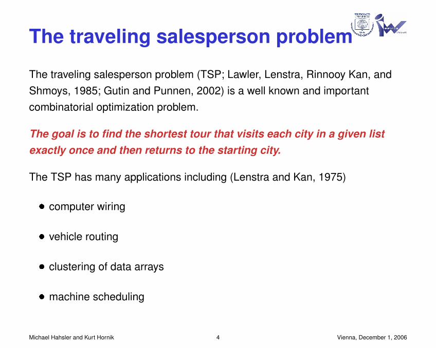
Some types of TSPs

Symmetric TSP with a symmetric distance matrix: d(i, j) = d(j, i)

Asymmetric TSP – the distances are not equal for all pairs of cities. Ariseswhen instead of spatial distances cost or time is used to form D.

Euclidean TSP with euclidean distances.

TSP with triangle inequality where d(i, j) + d(j, k) ≥ d(i, k).


Some algorithms and heuristics

Algorithms for exact solution

� Dynamic programming for small instances (Held and Karp, 1962).

� Branch-and bound, branch-and-cut,. . .

Heuristics

1. Tour construction

(a) Choose initial tour (e.g., random city, convex hull for Euclidean TSP)

(b) Selection method (nearest, farthest, arbitrary,. . . )

(c) Insertion method (minimum cost, greatest angle)

or solve assignment problem w/linear programming + patching

2. Tour improvement

� Edge exchange procedures: 2-opt (Croes, 1958), 3-opt (Lin, 1965),k-opt, Or-opt

� Variable r-opt (Lin and Kernighan, 1973)


The TSP package


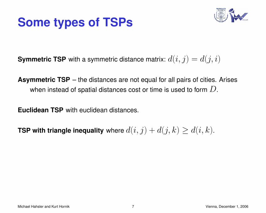
Overview

TSP/ATSP TOUR

dist matrix

TSPLIBfile

write_TSPLIB()

as.dist()TSP()/ATSP()

as.TSP()/as.ATSP()

integer (vector)

as.integer()cut_tour()

TSP()as.TSP()

as.matrix()

solve_TSP()

TOUR()as.TOUR()

read_TSPLIB()

Methods for TSP/ATSP: print(), n_of_cities(), labels(), image().Methods for TOUR: print(), labels(), cut_tour(), tour_length().


Solving (A)TSPs

Common interface:

solve_TSP(x, method, control)

where

� x is the TSP to be solved,

� method is a character string indicating the method used to solve the TSP,and

� control can contain a list with additional information used by the solver.


Currently available algorithms

The NP-completeness of the TSP makes it already for medium sized TSPinstances necessary to resort to heuristics. In TSP, we implemented somesimple heuristics described by Rosenkrantz, Stearns, and Philip M. Lewis(1977):

� Nearest neighbor algorithm

� Some variants of the insertion algorithm

The package also provides an interface to the Concorde TSPsolver (Applegate, Bixby, Chvátal, and Cook, 2000).


Nearest neighbor algorithm

The nearest neighbor algorithm (Rosenkrantz et al., 1977) follows a very simplegreedy procedure: The algorithm starts with a tour containing a randomlychosen city. Then the algorithm always adds to the last city in the tour thenearest not yet visited city. The algorithm stops when all cities are on the tour.This algorithm is implemented as method "nn" for solve_TSP().

An extension to this algorithm is to repeat it with each city as the starting pointand then return the best of the found tours. This algorithm is implemented asmethod "repetitive_nn".


Insertion algorithmsAll insertion algorithms (Rosenkrantz et al., 1977) start with a tour consisting of an arbitrary cityand then choose in each step a city k not yet on the tour. This city is inserted into the existingtour between two consecutive cities i and j, such that

d(i, k) + d(k, j)− d(i, j)

is minimized. The algorithms stops when all cities are on the tour. The insertion algorithms differin the way the city to be inserted next is chosen:

Nearest insertion The city k is chosen in each step as the city which is nearest to a city on thetour.

Farthest insertion The city k is chosen in each step as the city which is farthest to any of thecities on the tour.

Cheapest insertion The city k is chosen in each step such that the cost of inserting the newcity (i.e., the increase in the tour’s length) is minimal.

Arbitrary insertion The city k is chosen randomly from all cities not yet on the tour.

Methods: "nearest_insertion", "farthest_insertion", "cheapest_insertion","arbitrary_insertion"


Some properties of the insertion

algorithmsThe nearest and cheapest insertion algorithms are variants of to the minimumspanning tree algorithm which is known to be a good algorithm to find aHamiltonian cycle in a connected, undirected graph with a close to minimalweight sum. For nearest and cheapest insertion, adding a city to a partial tourcorresponds to adding an edge to a partial spanning tree. For TSPs withdistances obeying the triangular inequality , the upper bound for the length ofthe tour found by the minimum spanning tree algorithm is twice the optimaltour length.

The idea behind the farthest insertion algorithm is to link cities far outside intothe tour fist to establish an outline of the whole tour early. With this change, thealgorithm cannot be directly related to generating a minimum spanning tree andthus the upper bound stated above cannot be guaranteed. However, it can wasshown that the algorithm generates tours which approach 1.5 times theoptimal tour length (Johnson and Papadimitriou, 1985).


Concorde

Concorde (Applegate et al., 2000; Applegate, Bixby, Chvatal, and Cook, 2006)is currently one of the best implementations for solving symmetric TSPs basedon the branch-and-cut method.

In May 2004, Concorde was used to find the optimal solution for the TSP ofvisiting all 24,978 cities in Sweden. The computation was carried out on acluster with 96 nodes and took in total almost 100 CPU years (assuming asingle CPU Xeon 2.8 GHz processor).

TSP provides a simple interface to Concorde which is used for method"concorde". It saves the TSP using write_TSPLIB() and then calls theConcorde executable and reads back the resulting tour.


Examples


Comparing some heuristicsUSCA50 contains 50 cities in the USA and Canada as a TSP.

> library("TSP")

> data("USCA50")

> tsp <- USCA50

> tsp

object of class 'TSP'

50 cities (distance 'euclidean')

Calculate tours:

> methods <- c("nearest_insertion", "farthest_insertion",

+ "cheapest_insertion", "arbitrary_insertion", "nn",

+ "repetitive_nn")

> tours <- lapply(methods, FUN = function(m) solve_TSP(tsp,

+ method = m))

> names(tours) <- methods

> tours[[1]]

object of class 'TOUR'

result of method 'nearest_insertion' for 50 cities

tour length: 17413


Comparing some heuristics (cont.)> opt <- 14497

> dotchart(c(sapply(tours, FUN = attr, "tour_length"),

+ optimal = opt), xlab = "tour length", xlim = c(0,

+ 25000))

nearest_insertion

farthest_insertion

cheapest_insertion

arbitrary_insertion

nn

repetitive_nn

optimal

●

●

●

●

●

●

●

0 5000 10000 15000 20000 25000

tour length


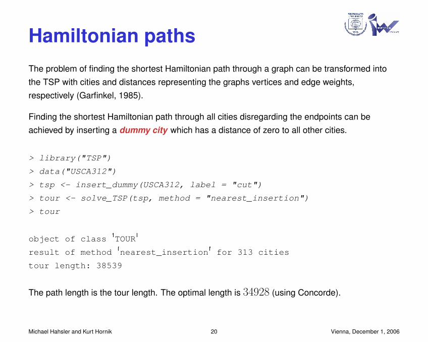
Hamiltonian pathsThe problem of finding the shortest Hamiltonian path through a graph can be transformed intothe TSP with cities and distances representing the graphs vertices and edge weights,respectively (Garfinkel, 1985).

Finding the shortest Hamiltonian path through all cities disregarding the endpoints can beachieved by inserting a dummy city which has a distance of zero to all other cities.

> library("TSP")

> data("USCA312")

> tsp <- insert_dummy(USCA312, label = "cut")

> tour <- solve_TSP(tsp, method = "nearest_insertion")

> tour



tour length: 38539

The path length is the tour length. The optimal length is 34928 (using Concorde).


Hamiltonian paths (cont.)

> path <- cut_tour(tour, "cut")

> head(labels(path))

[1] "Alert, NT" "Yellowknife, NT" "Dawson, YT"

[4] "Fairbanks, AK" "Nome, AK" "Anchorage, AK"

> tail(labels(path))

[1] "Eugene, OR" "Salem, OR" "Portland, OR" "Hilo, HI"

[5] "Honolulu, HI" "Lihue, HI"



Visualizing the path using maps et al.

> library("maps")

> library("sp")

> library("maptools")

> data("USCA312_map")

> plot_path <- function(path) {

+ plot(as(USCA312_coords, "Spatial"), axes = TRUE)

+ plot(USCA312_basemap, add = TRUE, col = "gray")

+ points(USCA312_coords, pch = 3, cex = 0.4, col = "red")

+ path_line <- SpatialLines(list(Lines(list(Line(USCA312_coords[path,

+ ])))))

+ plot(path_line, add = TRUE, col = "black")

+ points(USCA312_coords[c(head(path, 1), tail(path,

+ 1)), ], pch = 19, col = "black")

+ }


> plot_path(path)

160°°W 140°°W 120°°W 100°°W 80°°W 60°°W

20°°N

30°°N

40°°N

50°°N

60°°N

70°°N

80°°N

●

●


> plot_path(cut_tour(solve_TSP(tsp, method = "concorde"),

+ "cut"))

160°°W 140°°W 120°°W 100°°W 80°°W 60°°W

20°°N

30°°N

40°°N

50°°N

60°°N

70°°N

80°°N

●

●


Hamiltonian paths (cont.)Related Problem: Hamiltonian path starting with a given city (e.g., New York).Solution: All distances to the selected city are set to zero⇒ asymmetric TSP

> atsp <- as.ATSP(USCA312)

> ny <- which(labels(USCA312) == "New York, NY")

> atsp[, ny] <- 0

> tour <- solve_TSP(atsp, method = "nearest_insertion")

> tour



tour length: 41654

> path <- cut_tour(tour, ny, exclude_cut = FALSE)

> head(labels(path))

[1] "New York, NY" "Jersey City, NJ" "Newark, NJ"

[4] "Elizabeth, NJ" "Paterson, NJ" "White Plains, NY"

> tail(labels(path))

[1] "Anchorage, AK" "Nome, AK" "Fairbanks, AK"

[4] "Dawson, YT" "Yellowknife, NT" "Alert, NT"


> plot_path(path)

160°°W 140°°W 120°°W 100°°W 80°°W 60°°W

20°°N

30°°N

40°°N

50°°N

60°°N

70°°N

80°°N

●

●



Related Problem: Hamiltonian path with both end points given.Solution: This problem can be transformed to a TSP by replacing the two cities by a single citywhich contains the distances from the start point in the columns and the distances to the endpoint in the rows.

> m <- as.matrix(USCA312)

> ny <- which(labels(USCA312) == "New York, NY")

> la <- which(labels(USCA312) == "Los Angeles, CA")

> atsp <- ATSP(m[-c(ny, la), -c(ny, la)])

> atsp <- insert_dummy(atsp, label = "LA/NY")

> la_ny <- which(labels(atsp) == "LA/NY")

> atsp[la_ny, ] <- c(m[-c(ny, la), ny], 0)

> atsp[, la_ny] <- c(m[la, -c(ny, la)], 0)

> tour <- solve_TSP(atsp, method = "nearest_insertion")

> tour




tour length: 45094

> path_labels <- c("New York, NY", labels(cut_tour(tour,

+ la_ny)), "Los Angeles, CA")

> path_ids <- match(path_labels, labels(USCA312))

> head(path_labels)

[1] "New York, NY" "Central Islip, NY" "Albany, NY"

[4] "Schenectady, NY" "Troy, NY" "Pittsfield, MA"

> tail(path_labels)

[1] "Stockton, CA" "Lihue, HI" "Honolulu, HI"

[4] "Hilo, HI" "Santa Barbara, CA" "Los Angeles, CA"


> plot_path(path_ids)

160°°W 140°°W 120°°W 100°°W 80°°W 60°°W

20°°N

30°°N

40°°N

50°°N

60°°N

70°°N

80°°N

●

●


Rearrangement clustering

Climer and Zhang (2006) introduce rearrangement clustering by arranging all objects in a linearorder using a TSP. The authors suggest to find the cluster boundaries of k clusters by adding kdummy cities which have constant distance c to all other cities and are infinitely far from eachother.

> data("iris")

> tsp <- TSP(dist(iris[-5]), labels = iris[, "Species"])

> tsp_dummy <- insert_dummy(tsp, n = 2, label = "boundary")

> tour <- solve_TSP(tsp_dummy)

Next, we plot the TSP’s permuted distance matrix using shading to represent distances.

> image(tsp_dummy, tour)

> abline(h = which(labels(tour) == "boundary"), col = "red")

> abline(v = which(labels(tour) == "boundary"), col = "red")



> labels(tour)

[1] "virginica" "virginica" "virginica" "versicolor" "versicolor"[6] "versicolor" "virginica" "virginica" "versicolor" "versicolor"[11] "versicolor" "versicolor" "versicolor" "versicolor" "versicolor"[16] "versicolor" "versicolor" "versicolor" "versicolor" "versicolor"[21] "virginica" "versicolor" "virginica" "virginica" "virginica"[26] "virginica" "versicolor" "versicolor" "versicolor" "versicolor"[31] "versicolor" "versicolor" "versicolor" "versicolor" "versicolor"[36] "versicolor" "versicolor" "versicolor" "versicolor" "versicolor"[41] "versicolor" "versicolor" "versicolor" "versicolor" "versicolor"[46] "versicolor" "versicolor" "versicolor" "versicolor" "versicolor"[51] "versicolor" "virginica" "versicolor" "versicolor" "versicolor"[56] "versicolor" "versicolor" "versicolor" "versicolor" "versicolor"[61] "boundary" "setosa" "setosa" "setosa" "setosa"[66] "setosa" "setosa" "setosa" "setosa" "setosa"[71] "setosa" "setosa" "setosa" "setosa" "setosa"[76] "setosa" "setosa" "setosa" "setosa" "setosa"[81] "setosa" "setosa" "setosa" "setosa" "setosa"[86] "setosa" "setosa" "setosa" "setosa" "setosa"[91] "setosa" "setosa" "setosa" "setosa" "setosa"[96] "setosa" "setosa" "setosa" "setosa" "setosa"[101] "setosa" "setosa" "setosa" "setosa" "setosa"[106] "setosa" "setosa" "setosa" "setosa" "setosa"[111] "setosa" "boundary" "virginica" "virginica" "virginica"[116] "virginica" "virginica" "virginica" "virginica" "virginica"[121] "virginica" "virginica" "virginica" "virginica" "virginica"[126] "virginica" "virginica" "virginica" "virginica" "virginica"[131] "virginica" "virginica" "virginica" "virginica" "virginica"[136] "virginica" "virginica" "virginica" "virginica" "virginica"[141] "virginica" "virginica" "virginica" "virginica" "virginica"[146] "virginica" "virginica" "virginica" "virginica" "virginica"[151] "virginica" "versicolor"


ConclusionIn this paper we presented the package TSP which implements theinfrastructure to handle and solve TSPs. The package introduces classes forproblem descriptions (TSP and ATSP) and for the solution (TOUR). Togetherwith a simple interface for solving TSPs, it allows for an easy and transparentusage of the package.

With the interface to Concorde, TSP also can use a state of the artimplementation which efficiently computes exact solutions usingbranch-and-cut.


ReferencesD. Applegate, R. E. Bixby, V. Chvátal, and W. Cook. Tsp cuts which do not conform to the template paradigm. In M. Junger

and D. Naddef, editors, Computational Combinatorial Optimization, Optimal or Provably Near-Optimal Solutions,volume 2241 of Lecture Notes In Computer Science, pages 261–304, London, UK, 2000. Springer-Verlag.

D. Applegate, R. Bixby, V. Chvatal, and W. Cook. Concorde TSP Solver , 2006. URLhttp://www.tsp.gatech.edu/concorde/.

S. Climer and W. Zhang. Rearrangement clustering: Pitfalls, remedies, and applications. Journal of Machine LearningResearch, 7:919–943, June 2006.

G. A. Croes. A method for solving traveling-salesman problems. Operations Research, 6(6):791–812, 1958.

R. Garfinkel. Motivation and modeling. In Lawler et al. (1985).

G. Gutin and A. Punnen, editors. The Traveling Salesman Problem and Its Variations, volume 12 of CombinatorialOptimization. Kluwer, Dordrecht, 2002.

M. Held and R. Karp. A dynamic programming approach to sequencing problems. Journal of SIAM , 10:196–210, 1962.

A. Hoffman and P. Wolfe. History. In Lawler et al. (1985).

D. Johnson and C. Papadimitriou. Performance guarantees for heuristics. In Lawler et al. (1985).

E. L. Lawler, J. K. Lenstra, A. H. G. Rinnooy Kan, and D. B. Shmoys, editors. The traveling salesman problem. Wiley, NewYork, 1985.

J. Lenstra and A. R. Kan. Some simple applications of the travelling salesman problem. Operational Research Quarterly ,26(4):717–733, November 1975.

S. Lin. Computer solutions of the traveling-salesman problem. Bell System Technology Journal, 44:2245–2269, 1965.


http://www.tsp.gatech.edu/concorde/

S. Lin and B. Kernighan. An effective heuristic algorithm for the traveling-salesman problem. Operations Research, 21(2):498–516, 1973.

D. J. Rosenkrantz, R. E. Stearns, and I. Philip M. Lewis. An analysis of several heuristics for the traveling salesman problem.SIAM Journal on Computing, 6(3):563–581, 1977.


TSP – A R-Package for the Traveling Salesperson Problem · the TSP with cities and distances representing the graphs vertices and edge weights, respectively (Garﬁnkel, 1985).

Documents