TS 4273: Traffic Engineering Traffic Stream Traffic Stream Characteristics Characteristics

TS 4273: Traffic Engineering Traffic Stream Characteristics.
Dec 21, 2015
Welcome message from author
This document is posted to help you gain knowledge. Please leave a comment to let me know what you think about it! Share it to your friends and learn new things together.
Transcript
TS 4273: Traffic Engineering
Traffic Stream CharacteristicsTraffic Stream Characteristics
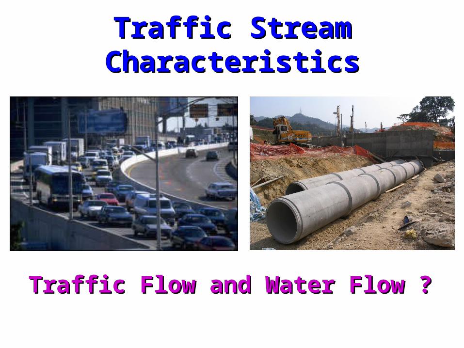
Traffic Stream CharacteristicsTraffic Stream Characteristics
Traffic Flow and Water Flow ?Traffic Flow and Water Flow ?
Type Of FacilitiesType Of Facilities
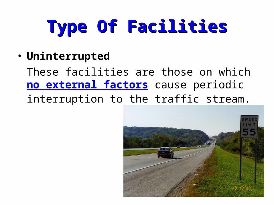
• Uninterrupted
These facilities are those on which no external factors cause periodic interruption to the traffic stream.

Type Of FacilitiesType Of Facilities
• Uninterrupted
Example: freeways, limited-access facilities, where there are no traffic signal, stop or yield signs, or surface intersections. It may also exist in long sections of rural highway between signalized intersections.
Type Of FacilitiesType Of Facilities
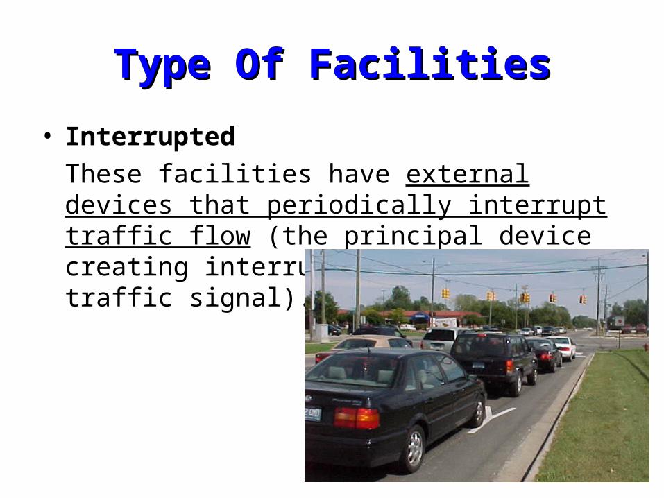
• Interrupted
These facilities have external devices that periodically interrupt traffic flow (the principal device creating interrupted flow is the traffic signal).
Traffic Stream ParametersTraffic Stream Parameters
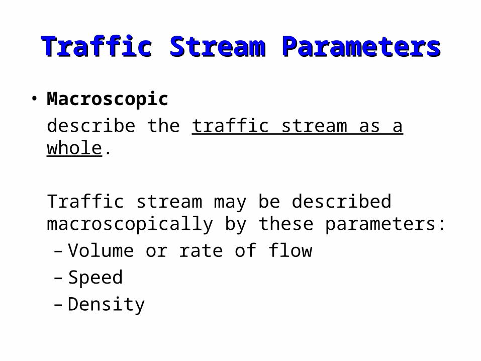
• Macroscopic
describe the traffic stream as a whole.
Traffic stream may be described macroscopically by these parameters: – Volume or rate of flow– Speed– Density
Traffic Stream ParametersTraffic Stream Parameters
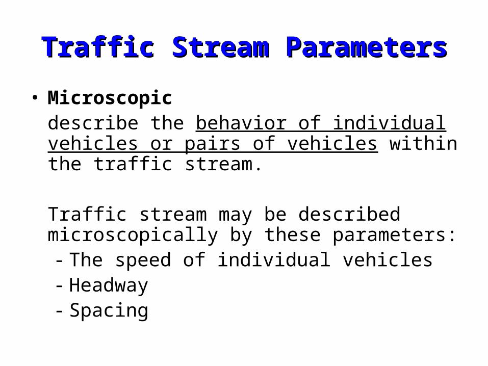
• Microscopicdescribe the behavior of individual vehicles or pairs of vehicles within the traffic stream.
Traffic stream may be described microscopically by these parameters: - The speed of individual vehicles- Headway - Spacing
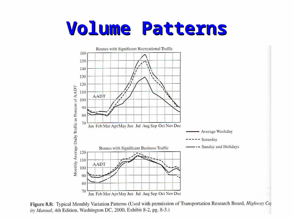
Volume PatternsVolume Patterns
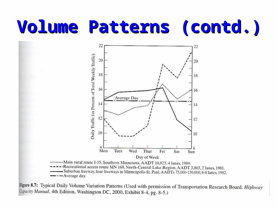
Volume Patterns (contd.)Volume Patterns (contd.)
Volume and Rate of FlowVolume and Rate of Flow
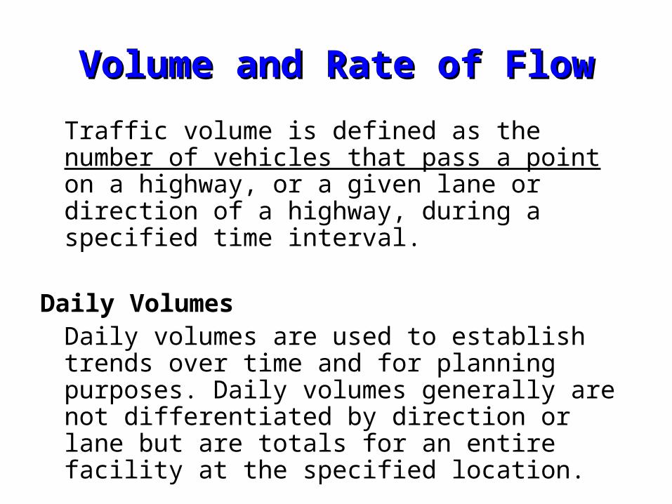
Traffic volume is defined as the number of vehicles that pass a point on a highway, or a given lane or direction of a highway, during a specified time interval.
Daily VolumesDaily volumes are used to establish trends over time and for planning purposes. Daily volumes generally are not differentiated by direction or lane but are totals for an entire facility at the specified location.
Volume and Rate of FlowVolume and Rate of Flow
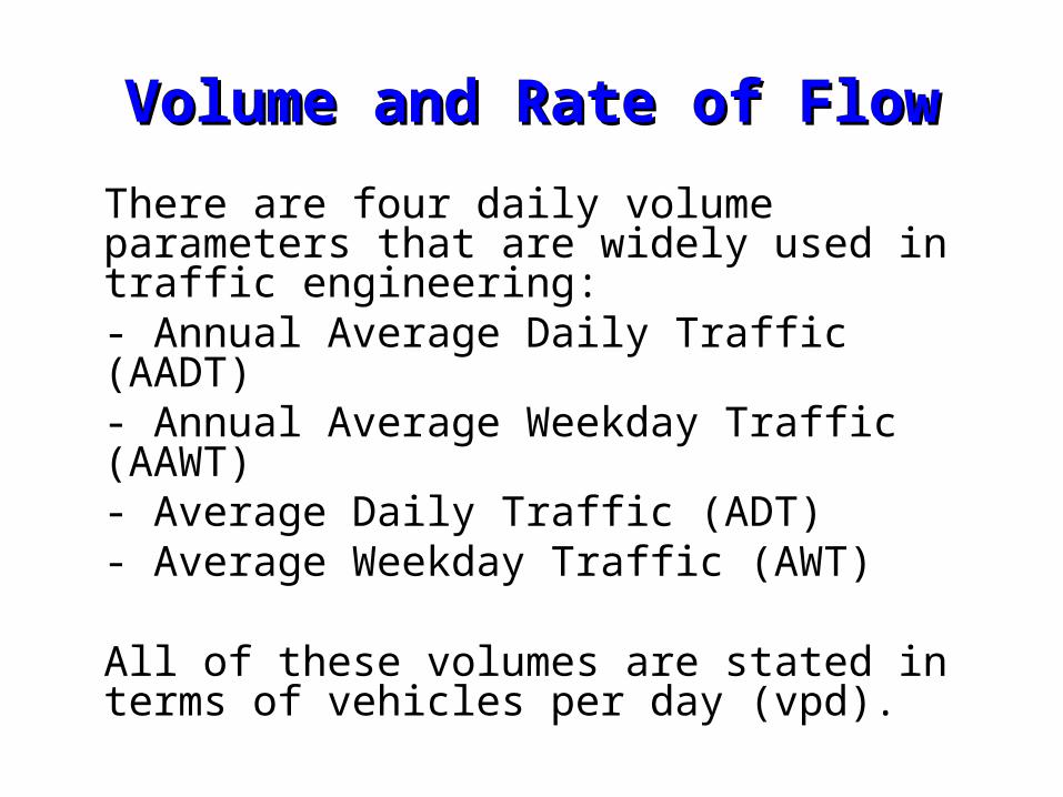
There are four daily volume parameters that are widely used in traffic engineering:- Annual Average Daily Traffic (AADT)- Annual Average Weekday Traffic (AAWT)- Average Daily Traffic (ADT)- Average Weekday Traffic (AWT)
All of these volumes are stated in terms of vehicles per day (vpd).
Daily VolumesDaily Volumes
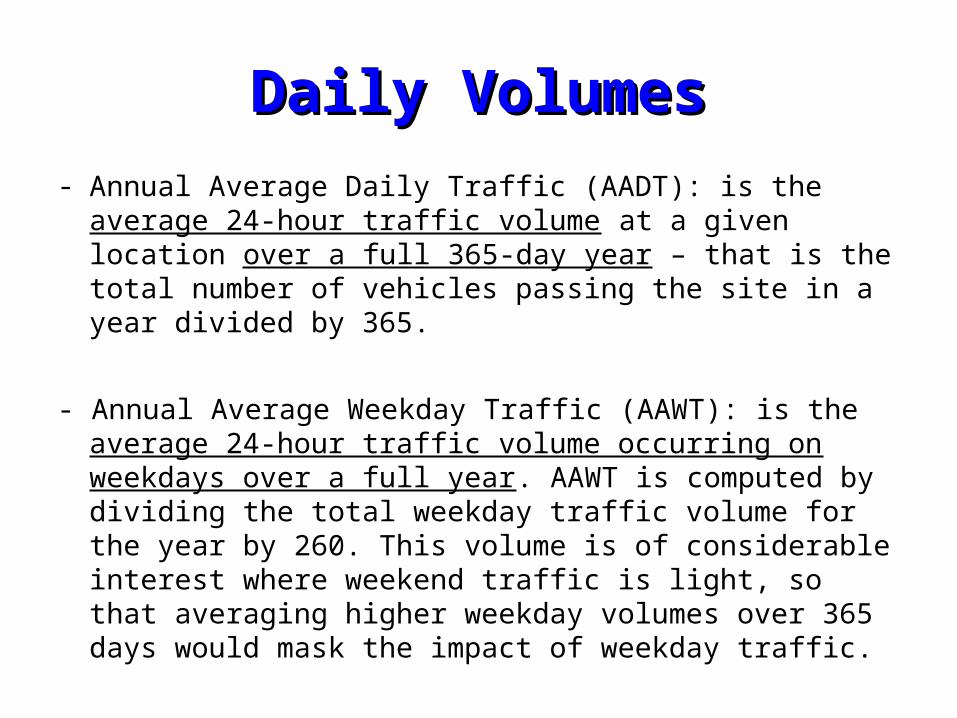
- Annual Average Daily Traffic (AADT): is the average 24-hour traffic volume at a given location over a full 365-day year – that is the total number of vehicles passing the site in a year divided by 365.
- Annual Average Weekday Traffic (AAWT): is the average 24-hour traffic volume occurring on weekdays over a full year. AAWT is computed by dividing the total weekday traffic volume for the year by 260. This volume is of considerable interest where weekend traffic is light, so that averaging higher weekday volumes over 365 days would mask the impact of weekday traffic.
Daily Volumes Daily Volumes (contd.)(contd.)
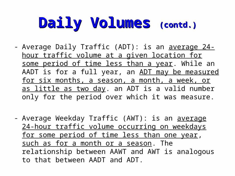
- Average Daily Traffic (ADT): is an average 24-hour traffic volume at a given location for some period of time less than a year. While an AADT is for a full year, an ADT may be measured for six months, a season, a month, a week, or as little as two day. an ADT is a valid number only for the period over which it was measure.
- Average Weekday Traffic (AWT): is an average 24-hour traffic volume occurring on weekdays for some period of time less than one year, such as for a month or a season. The relationship between AAWT and AWT is analogous to that between AADT and ADT.
Daily Volumes Daily Volumes (contd.)(contd.)
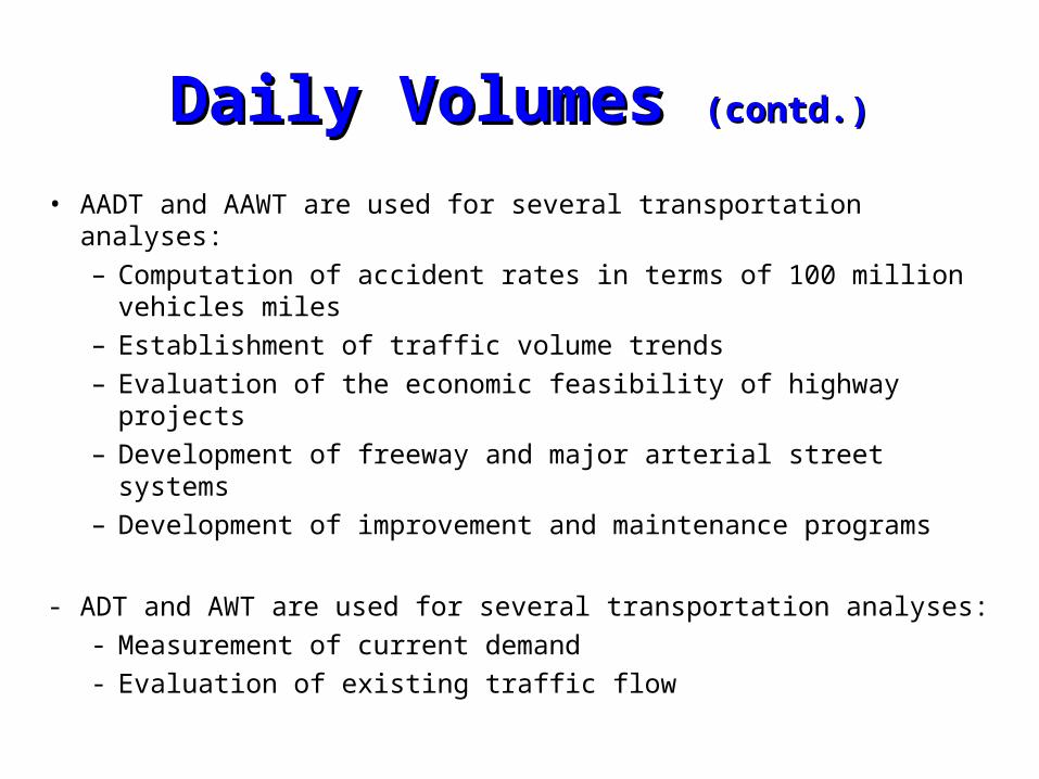
• AADT and AAWT are used for several transportation analyses:
– Computation of accident rates in terms of 100 million vehicles miles
– Establishment of traffic volume trends
– Evaluation of the economic feasibility of highway projects
– Development of freeway and major arterial street systems
– Development of improvement and maintenance programs
- ADT and AWT are used for several transportation analyses:
- Measurement of current demand
- Evaluation of existing traffic flow
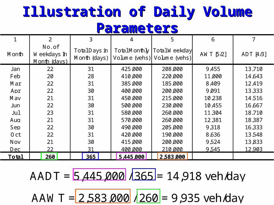
Illustration of Daily Volume ParametersIllustration of Daily Volume Parameters1 2 3 4 5 6 7
MonthNo. of
Weekdays In Month (days)
Total Days in Month (days)
Total Monthly Volume (vehs)
Total Weekday Volume (vehs)
AWT [5/2] ADT [4/3]
Jan 22 31 425,000 208,000 9,455 13,710Feb 20 28 410,000 220,000 11,000 14,643Mar 22 31 385,000 185,000 8,409 12,419Apr 22 30 400,000 200,000 9,091 13,333May 21 31 450,000 215,000 10,238 14,516Jun 22 30 500,000 230,000 10,455 16,667Jul 23 31 580,000 260,000 11,304 18,710Aug 21 31 570,000 260,000 12,381 18,387Sep 22 30 490,000 205,000 9,318 16,333Oct 22 31 420,000 190,000 8,636 13,548Nov 21 30 415,000 200,000 9,524 13,833Dec 22 31 400,000 210,000 9,545 12,903
Total 260 365 5,445,000 2,583,000
AADT = 5,445,000 / 365 = 14,918 veh/day
AAWT = 2,583,000 / 260 = 9,935 veh/day
Hourly VolumesHourly Volumes
Daily volumes, while useful for planning purposes, cannot be used alone for design or operational analysis purposes.
Volume varies considerably over the 24 hours of the day, with periods of maximum flow occurring during the morning and evening commuter “rush hours”.
Hourly VolumesHourly Volumes
The single hour of the day that has the highest hourly volume is referred to as the “peak hour”.
The traffic volume within this hour is of greatest interest to traffic engineers for design and operational analysis usage.
The peak-hour volume is generally stated as a directional volume (each direction of flow is counted separately).
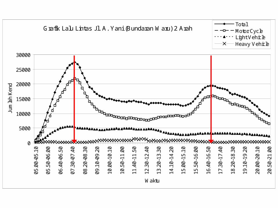
Grafik Lalu Lintas Jl. A. Yani (Bundaran Waru) 2 Arah
0
5000
10000
15000
20000
25000
30000
05.0
0-05
.10
05.5
0-06
.00
06.4
0-06
.50
07.3
0-07
.40
08.2
0-08
.30
09.1
0-09
.20
10.0
0-10
.10
10.5
0-11
.00
11.4
0-11
.50
12.3
0-12
.40
13.2
0-13
.30
14.1
0-14
.20
15.0
0-15
.10
15.5
0-16
.00
16.4
0-16
.50
17.3
0-17
.40
18.2
0-18
.30
19.1
0-19
.20
20.0
0-20
.10
20.5
0-21
.00
Waktu
Jum
lah
Ken
d
TotalMotor CycleLight VehicleHeavy Vehicle
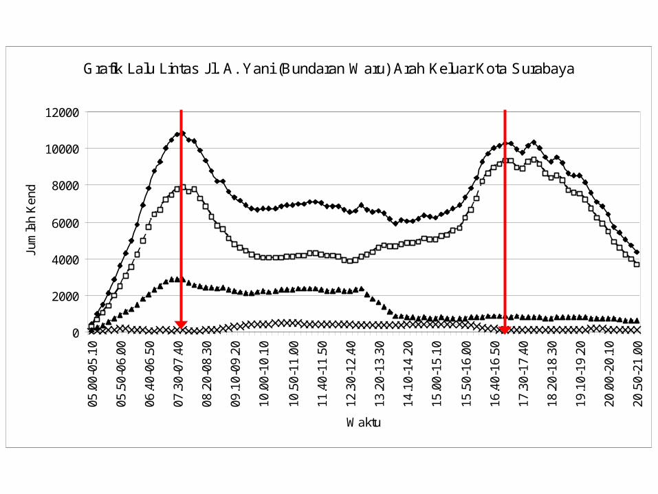
Grafik Lalu Lintas Jl. A. Yani (Bundaran Waru) Arah Keluar Kota Surabaya
0
2000
4000
6000
8000
10000
12000
05.0
0-05
.10
05.5
0-06
.00
06.4
0-06
.50
07.3
0-07
.40
08.2
0-08
.30
09.1
0-09
.20
10.0
0-10
.10
10.5
0-11
.00
11.4
0-11
.50
12.3
0-12
.40
13.2
0-13
.30
14.1
0-14
.20
15.0
0-15
.10
15.5
0-16
.00
16.4
0-16
.50
17.3
0-17
.40
18.2
0-18
.30
19.1
0-19
.20
20.0
0-20
.10
20.5
0-21
.00
Waktu
Jum
lah
Ken
d
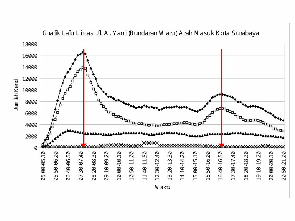
Grafik Lalu Lintas Jl. A. Yani (Bundaran Waru) Arah Masuk Kota Surabaya
0
2000
4000
6000
8000
10000
12000
14000
16000
1800005
.00-
05.1
0
05.5
0-06
.00
06.4
0-06
.50
07.3
0-07
.40
08.2
0-08
.30
09.1
0-09
.20
10.0
0-10
.10
10.5
0-11
.00
11.4
0-11
.50
12.3
0-12
.40
13.2
0-13
.30
14.1
0-14
.20
15.0
0-15
.10
15.5
0-16
.00
16.4
0-16
.50
17.3
0-17
.40
18.2
0-18
.30
19.1
0-19
.20
20.0
0-20
.10
20.5
0-21
.00
Waktu
Jum
lah
Ken
d
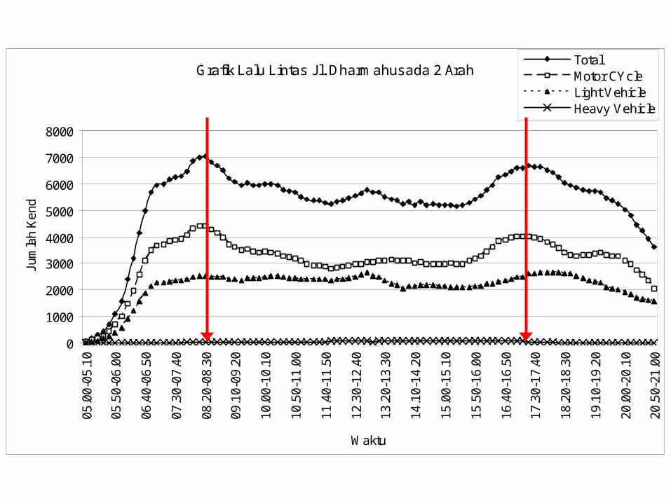
Grafik Lalu Lintas Jl. Dharmahusada 2 Arah
0
1000
2000
3000
4000
5000
6000
7000
8000
05.0
0-05
.10
05.5
0-06
.00
06.4
0-06
.50
07.3
0-07
.40
08.2
0-08
.30
09.1
0-09
.20
10.0
0-10
.10
10.5
0-11
.00
11.4
0-11
.50
12.3
0-12
.40
13.2
0-13
.30
14.1
0-14
.20
15.0
0-15
.10
15.5
0-16
.00
16.4
0-16
.50
17.3
0-17
.40
18.2
0-18
.30
19.1
0-19
.20
20.0
0-20
.10
20.5
0-21
.00
Waktu
Jum
lah
Ken
d
TotalMotor CYcleLight VehicleHeavy Vehicle

Grafik Lalu Lintas Jl. Dharmahusada Arah ke Timur
0
500
1000
1500
2000
2500
3000
3500
4000
4500
500005
.00-
05.1
0
05.5
0-06
.00
06.4
0-06
.50
07.3
0-07
.40
08.2
0-08
.30
09.1
0-09
.20
10.0
0-10
.10
10.5
0-11
.00
11.4
0-11
.50
12.3
0-12
.40
13.2
0-13
.30
14.1
0-14
.20
15.0
0-15
.10
15.5
0-16
.00
16.4
0-16
.50
17.3
0-17
.40
18.2
0-18
.30
19.1
0-19
.20
20.0
0-20
.10
20.5
0-21
.00
Waktu
Jum
lah
Ken
d
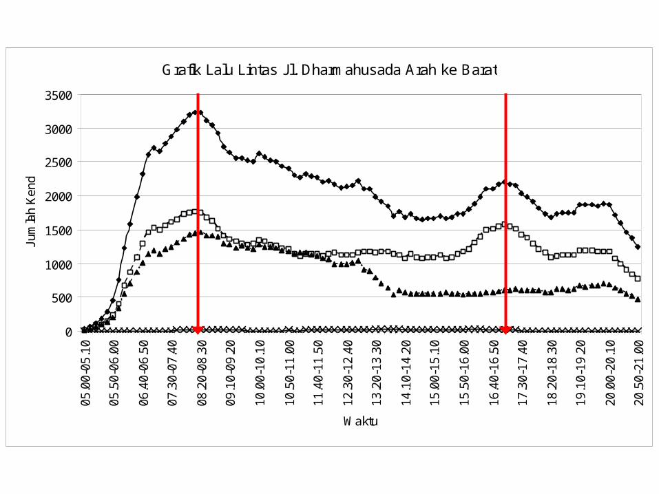
Grafik Lalu Lintas Jl. Dharmahusada Arah ke Barat
0
500
1000
1500
2000
2500
3000
350005
.00-
05.1
0
05.5
0-06
.00
06.4
0-06
.50
07.3
0-07
.40
08.2
0-08
.30
09.1
0-09
.20
10.0
0-10
.10
10.5
0-11
.00
11.4
0-11
.50
12.3
0-12
.40
13.2
0-13
.30
14.1
0-14
.20
15.0
0-15
.10
15.5
0-16
.00
16.4
0-16
.50
17.3
0-17
.40
18.2
0-18
.30
19.1
0-19
.20
20.0
0-20
.10
20.5
0-21
.00
Waktu
Jum
lah
Ken
d
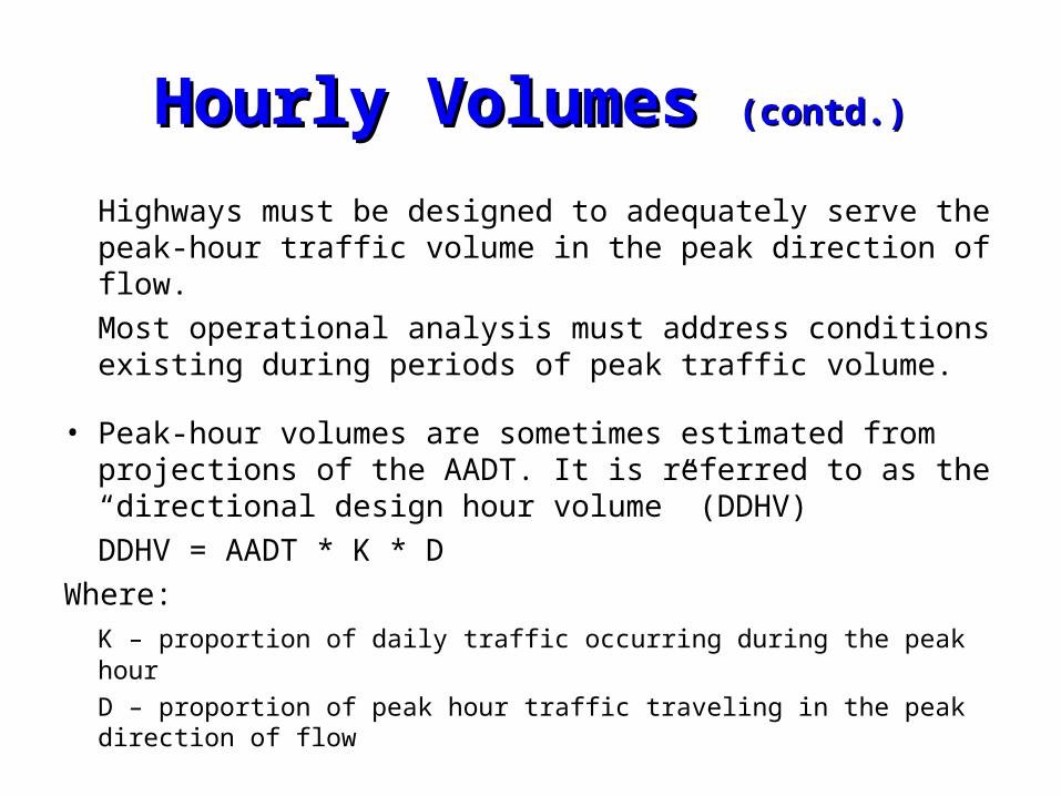
Hourly Volumes Hourly Volumes (contd.)(contd.)
Highways must be designed to adequately serve the peak-hour traffic volume in the peak direction of flow.
Most operational analysis must address conditions existing during periods of peak traffic volume.
• Peak-hour volumes are sometimes estimated from projections of the AADT. It is referred to as the “directional design hour volume” (DDHV)
DDHV = AADT * K * D
Where:
K – proportion of daily traffic occurring during the peak hour
D – proportion of peak hour traffic traveling in the peak direction of flow

Hourly Volumes Hourly Volumes (contd.)(contd.)
• Used for several transportation analyses:– Functional classification of roads– Design of geometric characteristics of highways (number
of lanes)– Capacity analysis– Development of programs related to traffic operations – Development of parking regulations
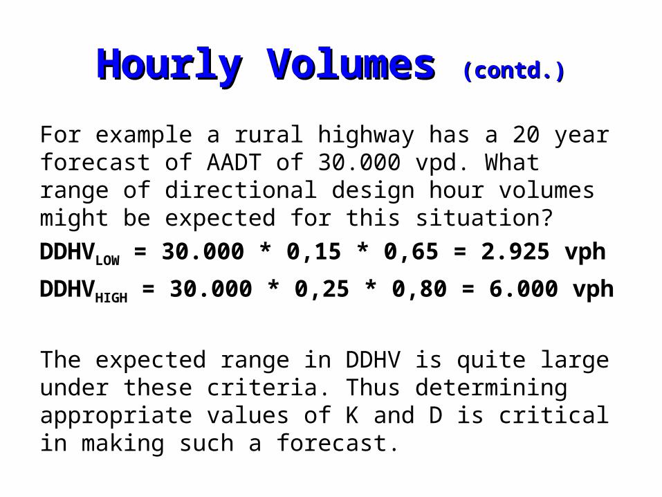
Hourly Volumes Hourly Volumes (contd.)(contd.)
For example a rural highway has a 20 year forecast of AADT of 30.000 vpd. What range of directional design hour volumes might be expected for this situation?
DDHVLOW = 30.000 * 0,15 * 0,65 = 2.925 vph
DDHVHIGH = 30.000 * 0,25 * 0,80 = 6.000 vph
The expected range in DDHV is quite large under these criteria. Thus determining appropriate values of K and D is critical in making such a forecast.
Sub Hourly VolumesSub Hourly VolumesWhile hourly traffic volumes form the basis for many forms of traffic design and analysis, the variation of traffic within given hour is also of considerable interest.
The quality of traffic flow is often related to short-term fluctuations in traffic demand. A facility may have sufficient capacity to serve the peak-hour demand, but short-term peaks of flow within the hour may exceed capacity and create breakdown.
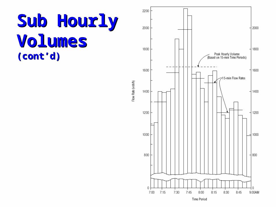
Sub Hourly Sub Hourly VolumesVolumes (cont’d)(cont’d)
Sub Hourly VolumesSub Hourly Volumes (cont’d)(cont’d)
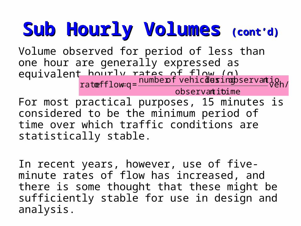
Volume observed for period of less than one hour are generally expressed as equivalent hourly rates of flow (q).
For most practical purposes, 15 minutes is considered to be the minimum period of time over which traffic conditions are statistically stable.
In recent years, however, use of five-minute rates of flow has increased, and there is some thought that these might be sufficiently stable for use in design and analysis.
veh/hn timeobservatio
nobservatio during vehiclesofnumber =qflow of rate
Sub Hourly VolumesSub Hourly Volumes (cont’d)(cont’d)
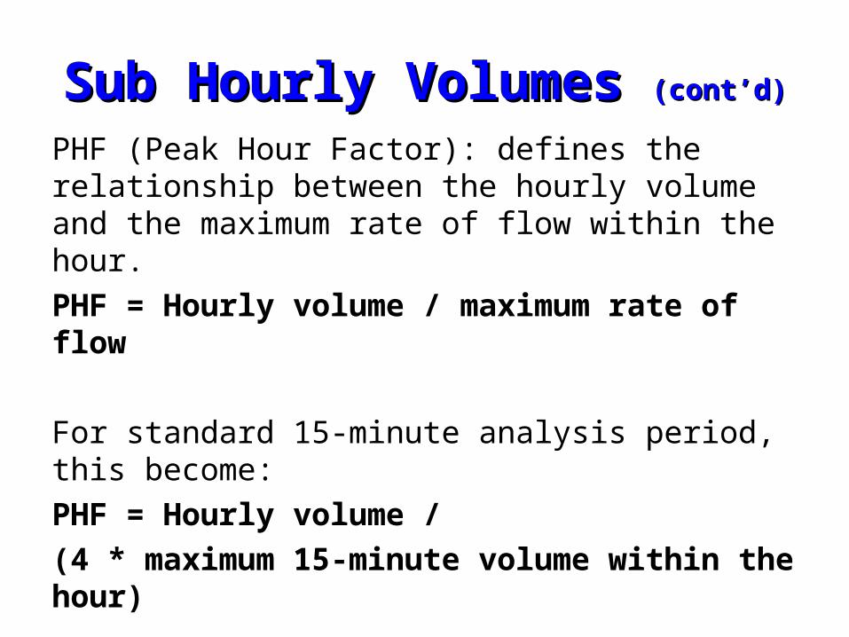
PHF (Peak Hour Factor): defines the relationship between the hourly volume and the maximum rate of flow within the hour.
PHF = Hourly volume / maximum rate of flow
For standard 15-minute analysis period, this become:
PHF = Hourly volume /
(4 * maximum 15-minute volume within the hour)
Sub hourly Volumes Sub hourly Volumes (contd.)(contd.)
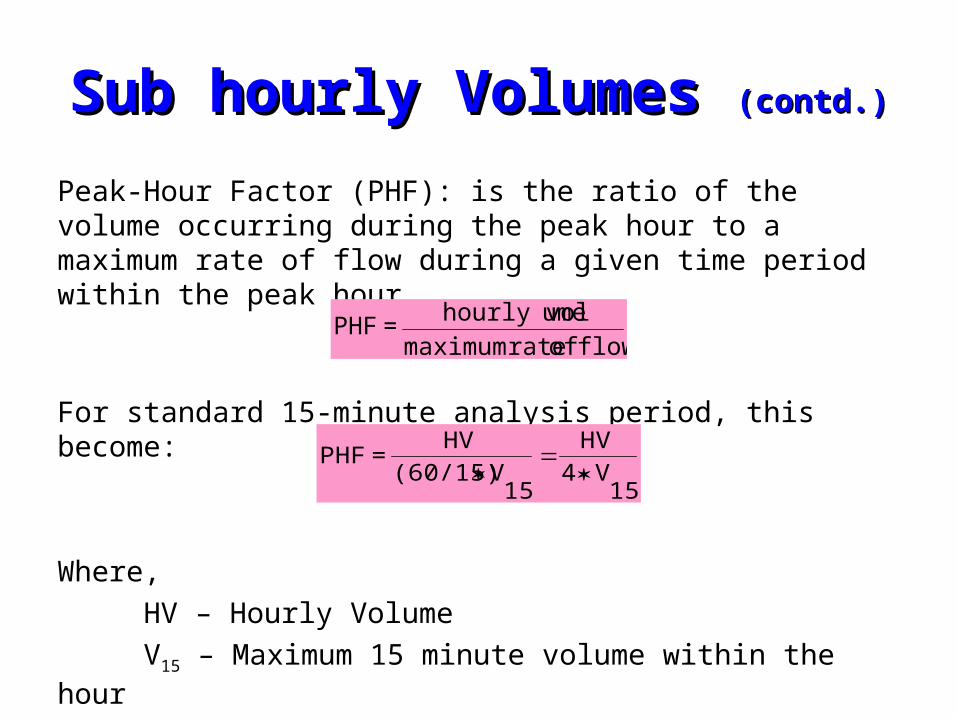
Peak-Hour Factor (PHF): is the ratio of the volume occurring during the peak hour to a maximum rate of flow during a given time period within the peak hour
For standard 15-minute analysis period, this become:
Where,
HV – Hourly Volume
V15 – Maximum 15 minute volume within the hour
flow of rate maximum
umehourly vol = PHF
15V4
HV
15V(60/15)
HV = PHF
Sub Hourly Volumes Sub Hourly Volumes (contd.)(contd.)
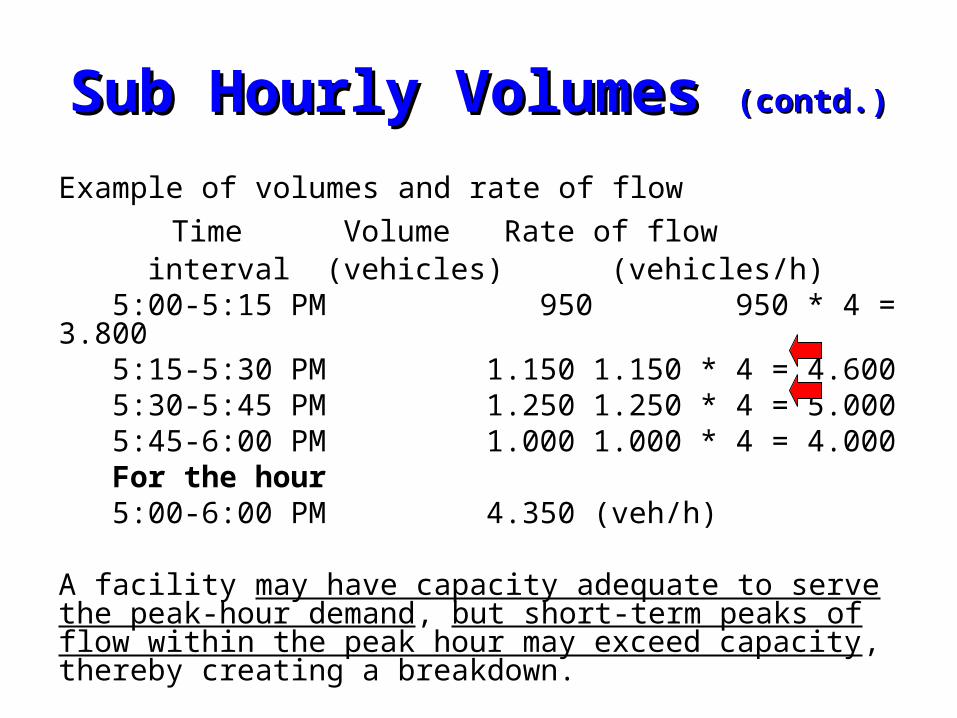
Example of volumes and rate of flow
Time Volume Rate of flowinterval (vehicles) (vehicles/h)
5:00-5:15 PM 950 950 * 4 = 3.800 5:15-5:30 PM 1.150 1.150 * 4 = 4.600 5:30-5:45 PM 1.250 1.250 * 4 = 5.000 5:45-6:00 PM 1.000 1.000 * 4 = 4.000 For the hour 5:00-6:00 PM 4.350 (veh/h)
A facility may have capacity adequate to serve the peak-hour demand, but short-term peaks of flow within the peak hour may exceed capacity, thereby creating a breakdown.
Sub hourly Volumes Sub hourly Volumes (contd.)(contd.)
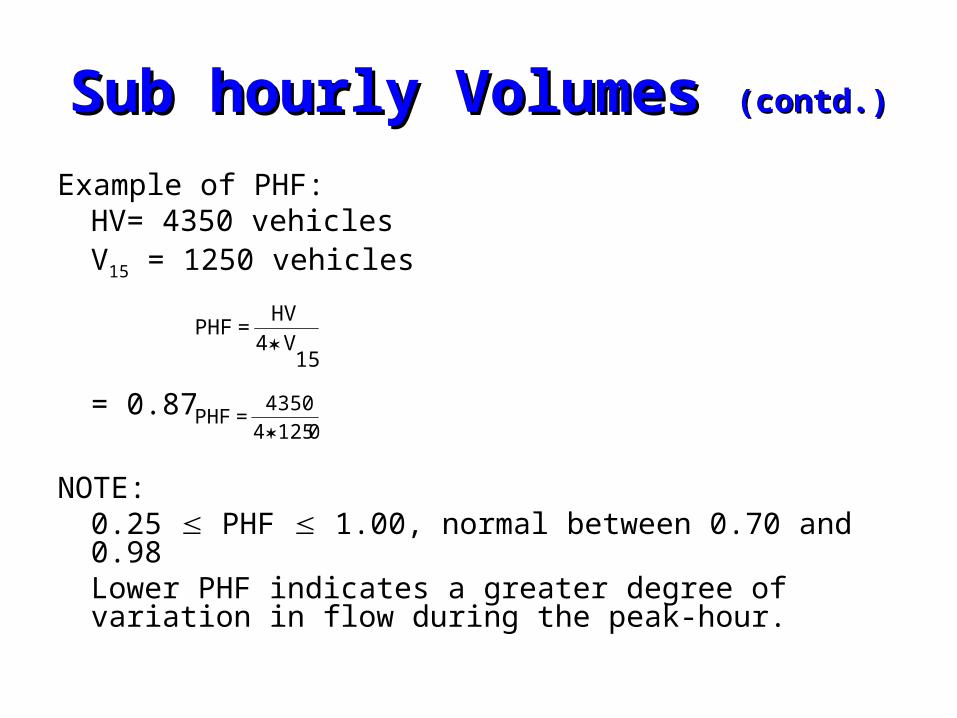
Example of PHF:HV= 4350 vehiclesV15 = 1250 vehicles
= 0.87
NOTE:0.25 PHF 1.00, normal between 0.70 and 0.98Lower PHF indicates a greater degree of variation in flow during the peak-hour.
01254
4350 = PHF
15V4
HV = PHF
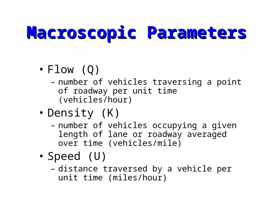
Macroscopic ParametersMacroscopic Parameters
• Flow (Q)– number of vehicles traversing a point of
roadway per unit time (vehicles/hour)
• Density (K)– number of vehicles occupying a given length
of lane or roadway averaged over time (vehicles/mile)
• Speed (U)– distance traversed by a vehicle per unit time
(miles/hour)
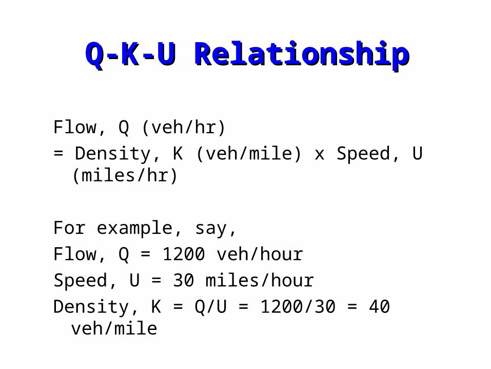
Q-K-U RelationshipQ-K-U Relationship
Flow, Q (veh/hr)
= Density, K (veh/mile) x Speed, U (miles/hr)
For example, say,
Flow, Q = 1200 veh/hour
Speed, U = 30 miles/hour
Density, K = Q/U = 1200/30 = 40 veh/mile
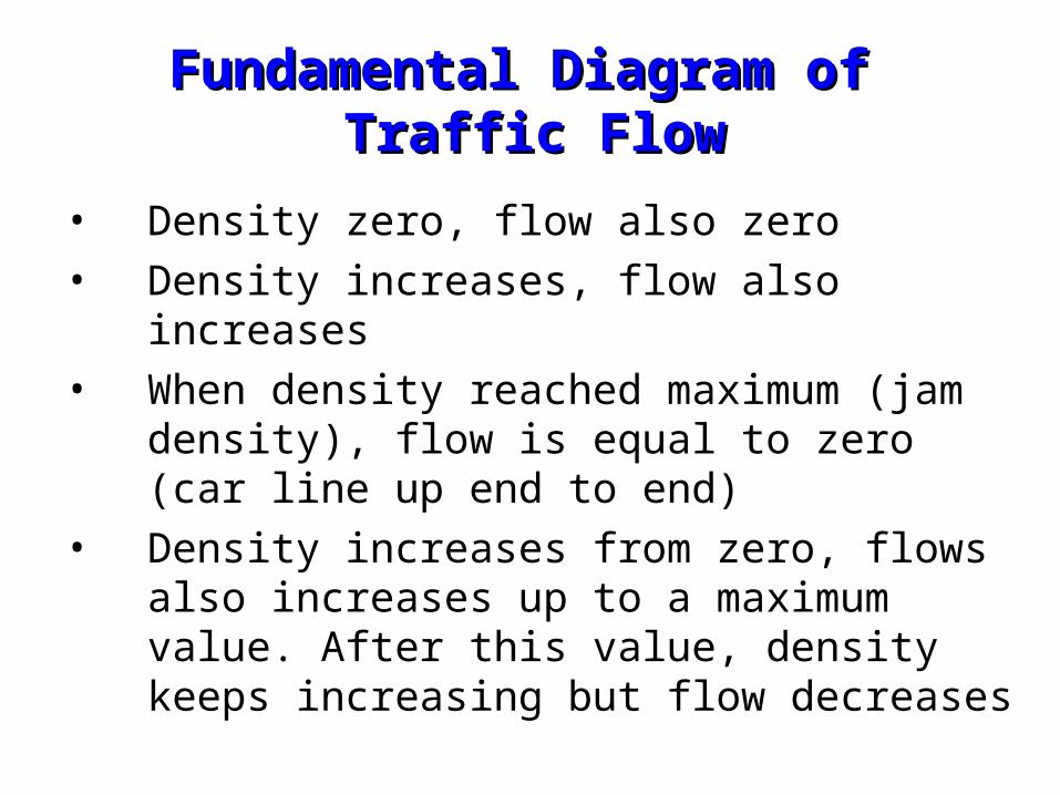
Fundamental Diagram of Traffic FlowFundamental Diagram of Traffic Flow
• Density zero, flow also zero• Density increases, flow also increases• When density reached maximum (jam density),
flow is equal to zero (car line up end to end)• Density increases from zero, flows also
increases up to a maximum value. After this value, density keeps increasing but flow decreases
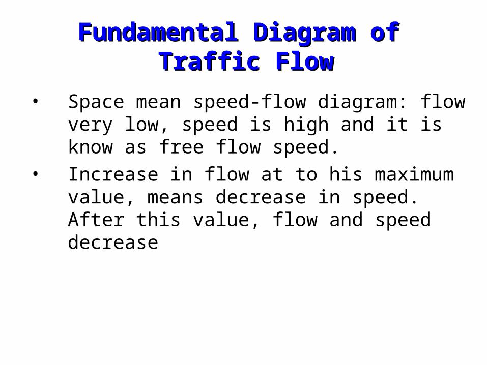
• Space mean speed-flow diagram: flow very low, speed is high and it is know as free flow speed.
• Increase in flow at to his maximum value, means decrease in speed. After this value, flow and speed decrease
Fundamental Diagram of Traffic FlowFundamental Diagram of Traffic Flow

Q-K-U RelationshipQ-K-U Relationship
Maximum Flow
Flo
w (
veh
/hr)
Density (veh/mile)
Sp
eed
(m
iles/h
r)
Flow (veh/hr)
Jam Density
Critical Density
Critical Density
Critical Speed
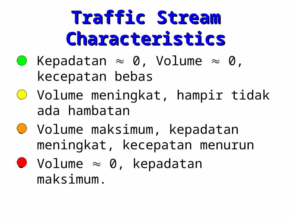
Traffic Stream CharacteristicsTraffic Stream Characteristics
o Kepadatan 0, Volume 0, kecepatan bebas
o Volume meningkat, hampir tidak ada hambatan
o Volume maksimum, kepadatan meningkat, kecepatan menurun
o Volume 0, kepadatan maksimum.
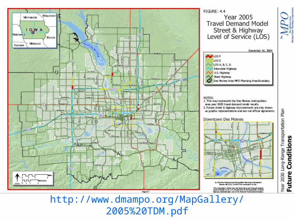
http://www.dmampo.org/MapGallery/2005%20TDM.pdf
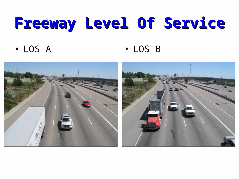
Freeway Level Of ServiceFreeway Level Of Service
• LOS A • LOS B
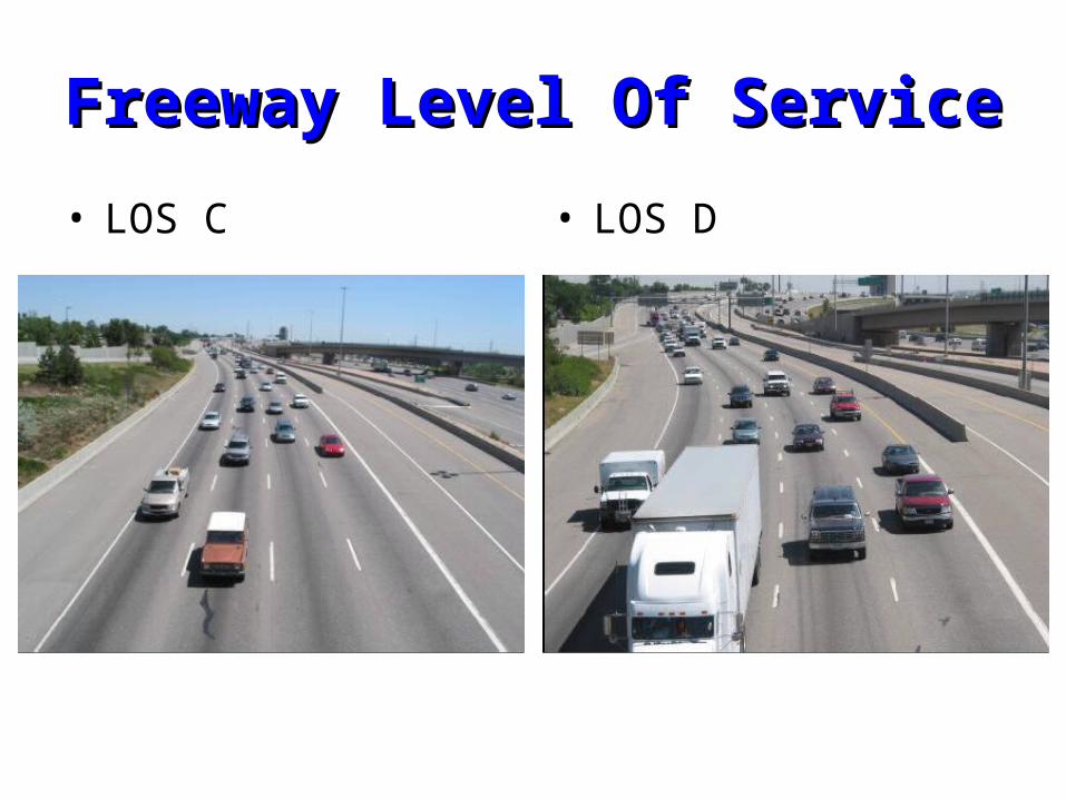
Freeway Level Of ServiceFreeway Level Of Service
• LOS C • LOS D
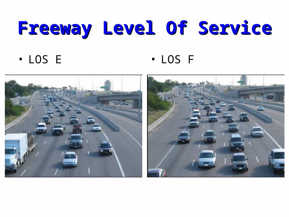
Freeway Level Of ServiceFreeway Level Of Service
• LOS E • LOS F
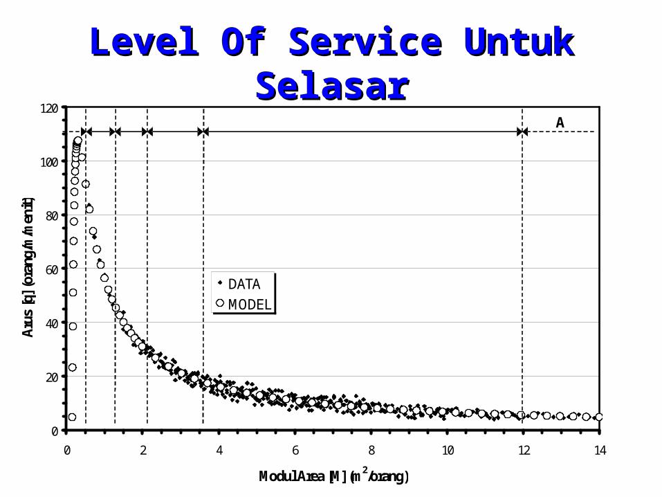
0
20
40
60
80
100
120
0 2 4 6 8 10 12 14
Modul Area [M] (m2/orang)
Aru
s [q
] (or
ang/
m/m
enit)
DATAMODEL
ABCDEF
Level Of Service Untuk SelasarLevel Of Service Untuk Selasar
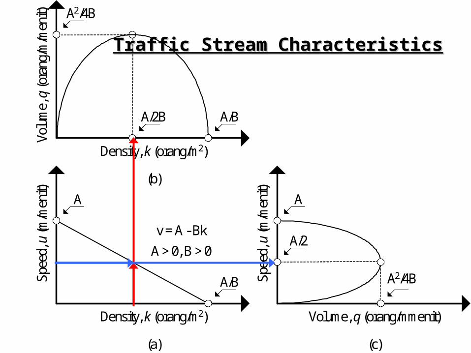
Traffic Stream CharacteristicsTraffic Stream Characteristics
A2/4B
A
Spee
d, u
(m/m
enit)
Volume, q (orang/mmenit)
A/2
(c)
A/B
A
Spee
d, u
(m/m
enit)
Density, k (orang/m2)
v = A - BkA > 0, B > 0
(a)
Density, k (orang/m2)
A/2B
A2/4B
Volu
me,
q (o
rang
/m/m
enit)
A/B
(b)
Traffic Stream ParametersTraffic Stream Parameters
• Volume and Rate of Flow
• Speed and Travel Time
• Density and Occupancy
• Spacing and Headway

SPEEDSPEED
• Space Mean Speed
• vs = average travel speed or space mean speed (kph)
• L = length of the highway segment (km)
• ti = travel time of the ith vehicle to cross the section (hours)
• n = number of travel times observed
n
ii
n
i
is
t
nL
n
tL
v
11
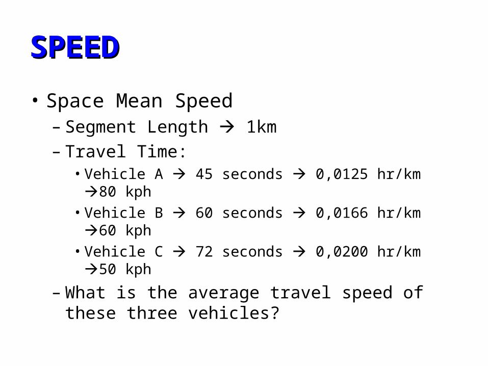
SPEEDSPEED
• Space Mean Speed– Segment Length 1km– Travel Time:
• Vehicle A 45 seconds 0,0125 hr/km 80 kph• Vehicle B 60 seconds 0,0166 hr/km 60 kph• Vehicle C 72 seconds 0,0200 hr/km 50 kph
– What is the average travel speed of these three vehicles?
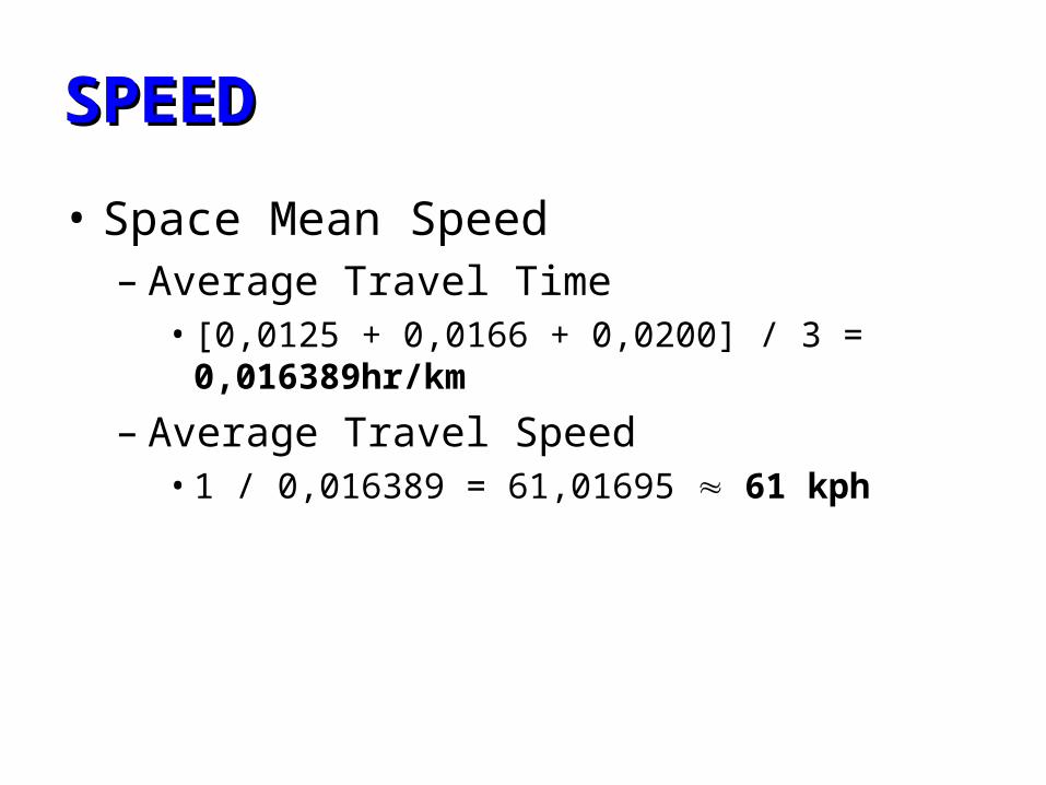
SPEEDSPEED
• Space Mean Speed– Average Travel Time
• [0,0125 + 0,0166 + 0,0200] / 3 = 0,016389hr/km
– Average Travel Speed• 1 / 0,016389 = 61,01695 61 kph
SPEEDSPEED
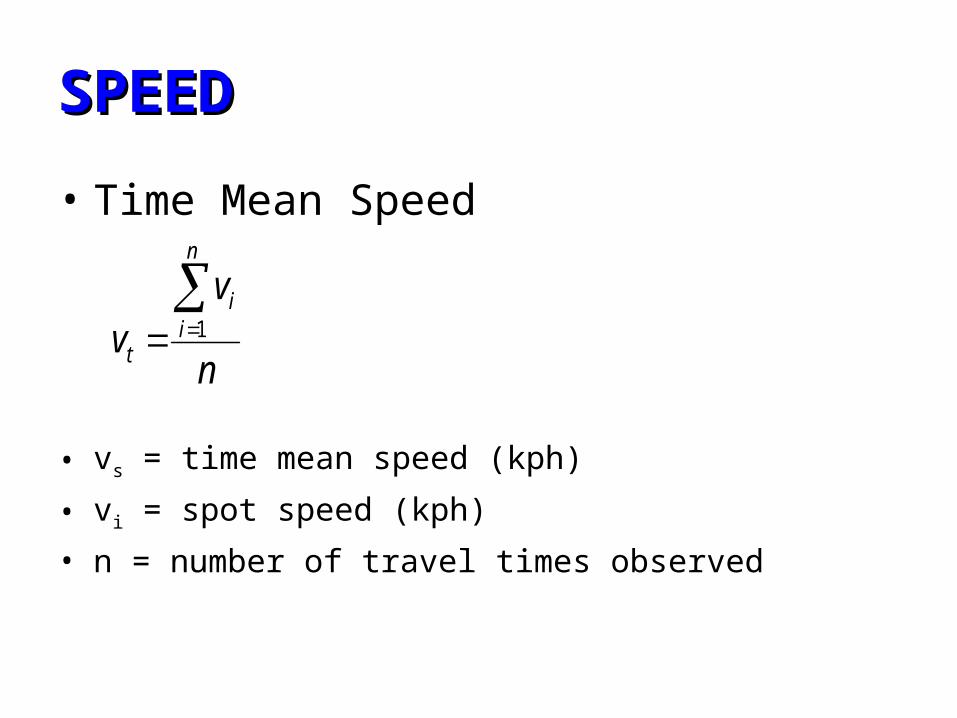
• Time Mean Speed
• vs = time mean speed (kph)
• vi = spot speed (kph)
• n = number of travel times observed
n
vv
n
ii
t
1
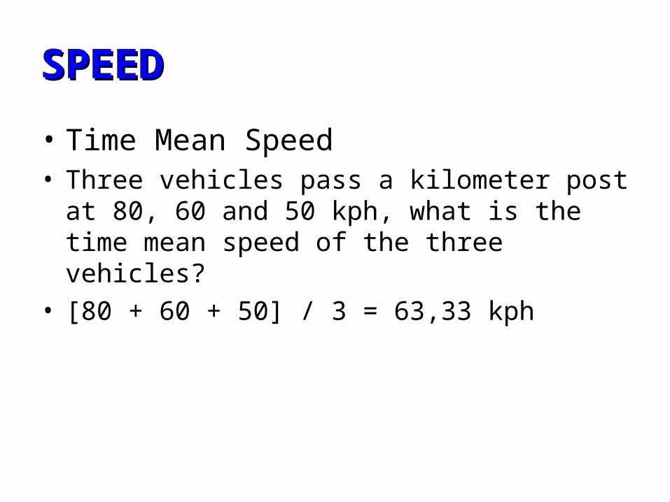
SPEED SPEED
• Time Mean Speed• Three vehicles pass a kilometer post at 80, 60
and 50 kph, what is the time mean speed of the three vehicles?
• [80 + 60 + 50] / 3 = 63,33 kph
SPEED SPEED
• Time Mean Speed (TMS)Kecepatan individu yang melintas suatu segmen selama periode waktu tertentu
SPEED SPEED
• Space Mean Speed (SMS)Kecepatan individu (TMS) dikonversi menjadi waktu tempuh, kemudian dihitung waktu tempuh rata-rata, kemudian dihitung kecepatan rata-rata.
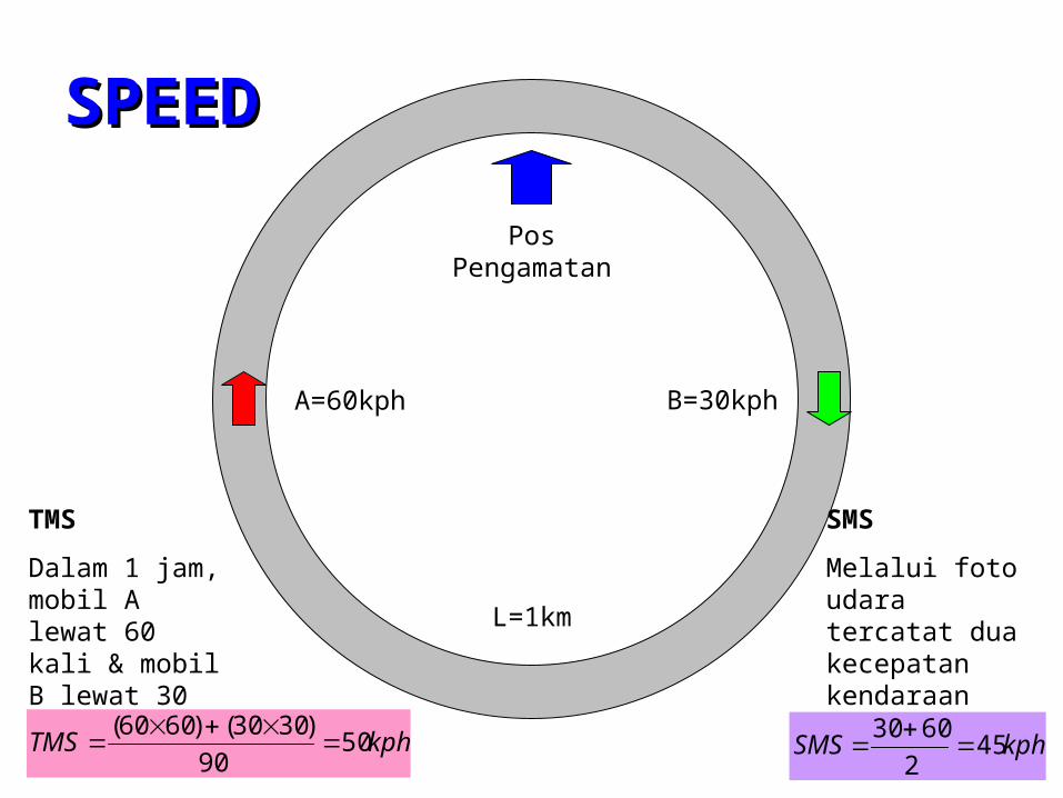
SPEED SPEED
A=60kph B=30kph
L=1km
TMS
Dalam 1 jam, mobil A lewat 60 kali & mobil B lewat 30 kali
Pos Pengamatan
kphTMS 5090
)3030()6060(
SMS
Melalui foto udara tercatat dua kecepatan kendaraan pada suatu ruang
kphSMS 452
6030
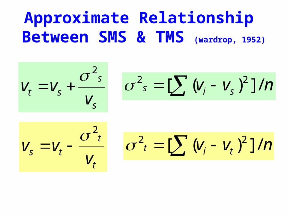
Approximate Relationship Between SMS & TMS (wardrop, 1952)
s
s
st vvv
2
t
t
ts vvv
2
nvv sis /])([ 22
nvv tit /])([ 22
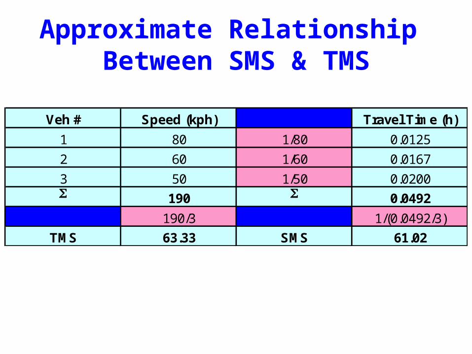
Approximate Relationship Between SMS & TMS
Veh # Speed (kph) Travel Time (h)
1 80 1/80 0.0125
2 60 1/60 0.0167
3 50 1/50 0.0200S 190 S 0.0492
190/3 1/(0.0492/3)
TMS 63.33 SMS 61.02
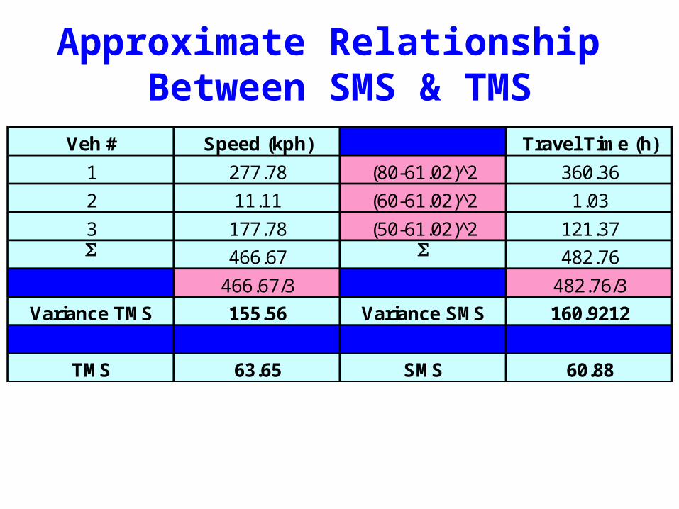
Approximate Relationship Between SMS & TMS
Veh # Speed (kph) Travel Time (h)
1 277.78 (80-61.02)^2 360.36
2 11.11 (60-61.02)^2 1.03
3 177.78 (50-61.02)^2 121.37S 466.67 S 482.76
466.67/3 482.76/3
Variance TMS 155.56 Variance SMS 160.9212
TMS 63.65 SMS 60.88
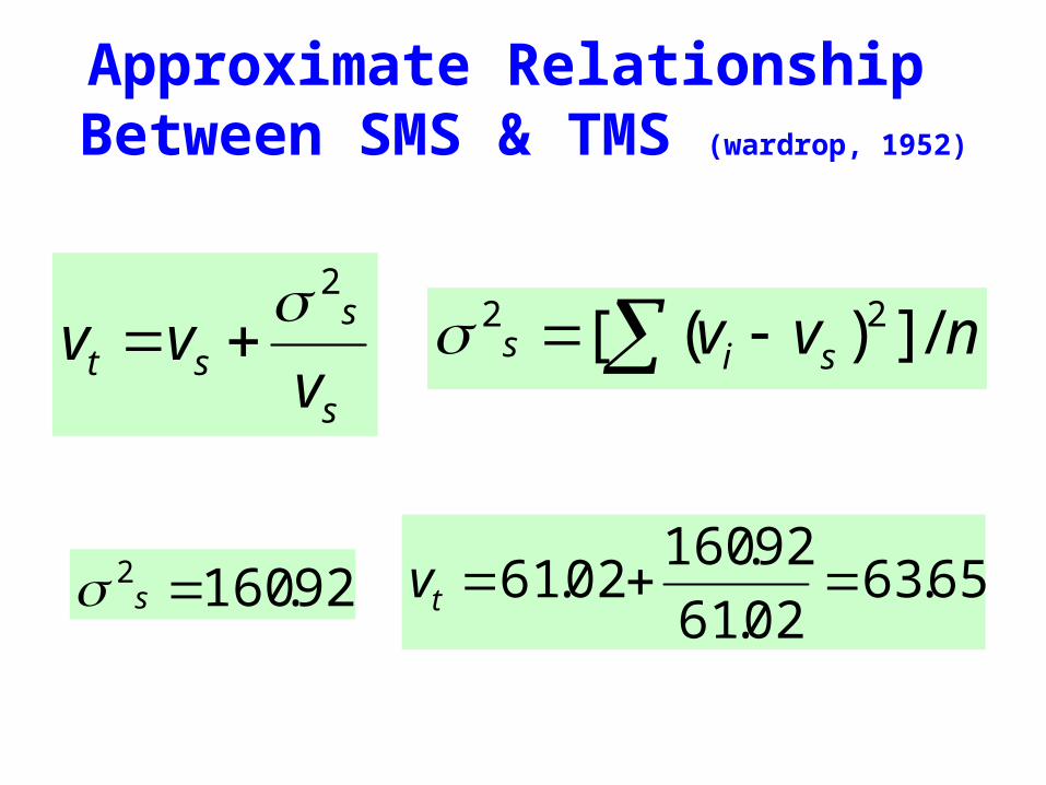
Approximate Relationship Between SMS & TMS (wardrop, 1952)
65.6302.61
92.16002.61 tv92.1602 s
s
s
st vvv
2 nvv sis /])([ 22
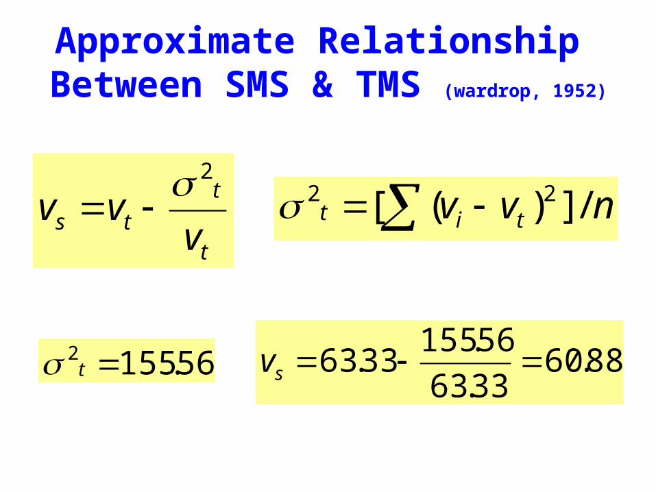
Approximate Relationship Between SMS & TMS (wardrop, 1952)
88.6033.63
56.15533.63 sv56.1552 t
t
t
ts vvv
2 nvv tit /])([ 22
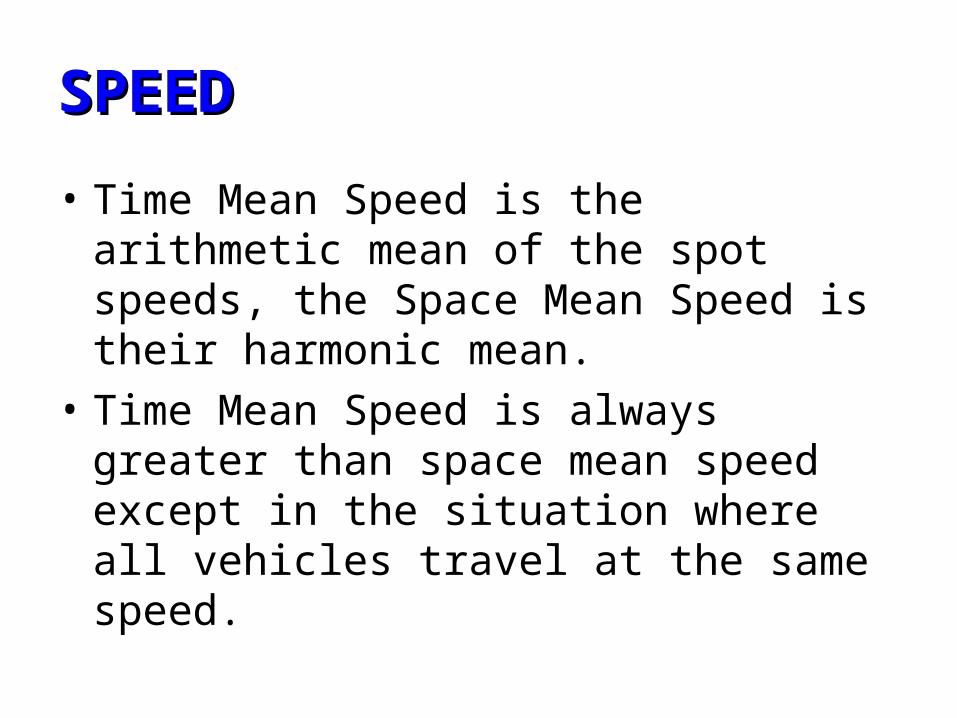
SPEED SPEED
• Time Mean Speed is the arithmetic mean of the spot speeds, the Space Mean Speed is their harmonic mean.
• Time Mean Speed is always greater than space mean speed except in the situation where all vehicles travel at the same speed.
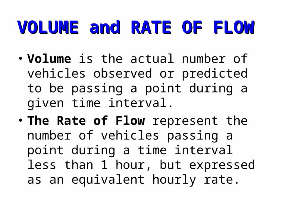
VOLUME and RATE OF FLOWVOLUME and RATE OF FLOW
• Volume is the actual number of vehicles observed or predicted to be passing a point during a given time interval.
• The Rate of Flow represent the number of vehicles passing a point during a time interval less than 1 hour, but expressed as an equivalent hourly rate.
VOLUME and RATE OF FLOWVOLUME and RATE OF FLOW
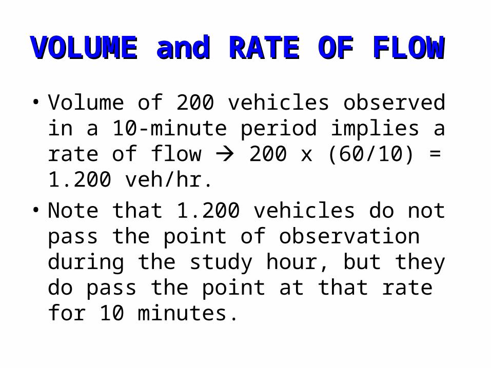
• Volume of 200 vehicles observed in a 10-minute period implies a rate of flow 200 x (60/10) = 1.200 veh/hr.
• Note that 1.200 vehicles do not pass the point of observation during the study hour, but they do pass the point at that rate for 10 minutes.
VOLUME and RATE OF FLOWVOLUME and RATE OF FLOW
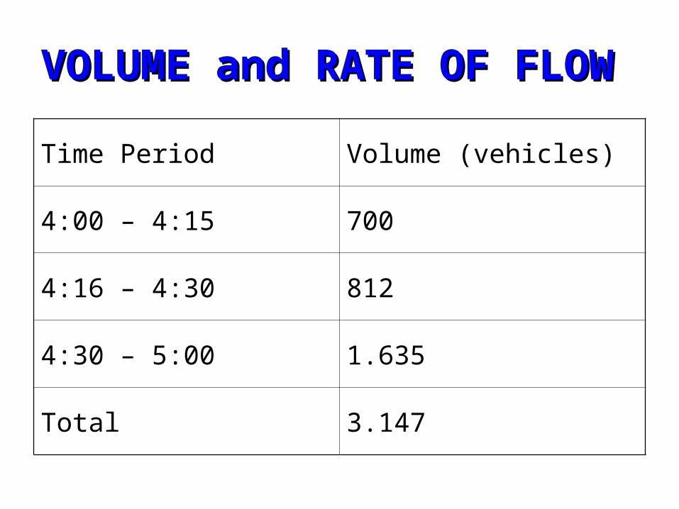
Time Period Volume (vehicles)
4:00 – 4:15 700
4:16 – 4:30 812
4:30 – 5:00 1.635
Total 3.147
VOLUME and RATE OF FLOWVOLUME and RATE OF FLOW
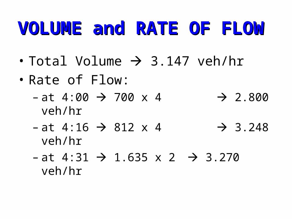
• Total Volume 3.147 veh/hr
• Rate of Flow:– at 4:00 700 x 4 2.800 veh/hr– at 4:16 812 x 4 3.248 veh/hr– at 4:31 1.635 x 2 3.270 veh/hr
DENSITYDENSITY
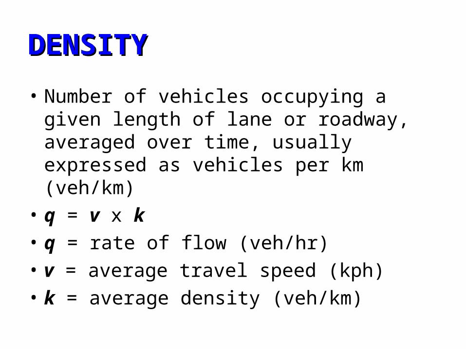
• Number of vehicles occupying a given length of lane or roadway, averaged over time, usually expressed as vehicles per km (veh/km)
• q = v x k
• q = rate of flow (veh/hr)
• v = average travel speed (kph)
• k = average density (veh/km)
DENSITYDENSITY
• A highway segment with a rate of flow of 1.350 veh/hr and an average travel speed of 45 kph would have a density of k = 1.350 / 45 = 30 veh/km.
• The proximity of vehicles in a traffic stream is given by density, which is a critical parameter in describing freedom of maneuverability.
SPACING and HEADWAYSPACING and HEADWAY
• Spacing (s) is defined as the distance between successive vehicles in a traffic stream as measured from front bumper to front bumper.
• Spacings of vehicles in a traffic lane can be generally observed from aerial photographs.
SPACING and HEADWAYSPACING and HEADWAY
• Headway is the corresponding time between successive vehicles as they pass a point on a roadway.
• Headways of vehicles can be measured using stopwatch observations as vehicles pass a point on a lane.
SPACING and HEADWAYSPACING and HEADWAY
• Average density (k), veh/km =
1.000, m/km / average spacing (s), m/veh
• Average headway (h), sec/veh =
average spacing (s), m/veh / average speed (v), m/sec
• Average Flow Rate (q), veh/hr =
3600, sec/hr / average headway (h), sec/hr
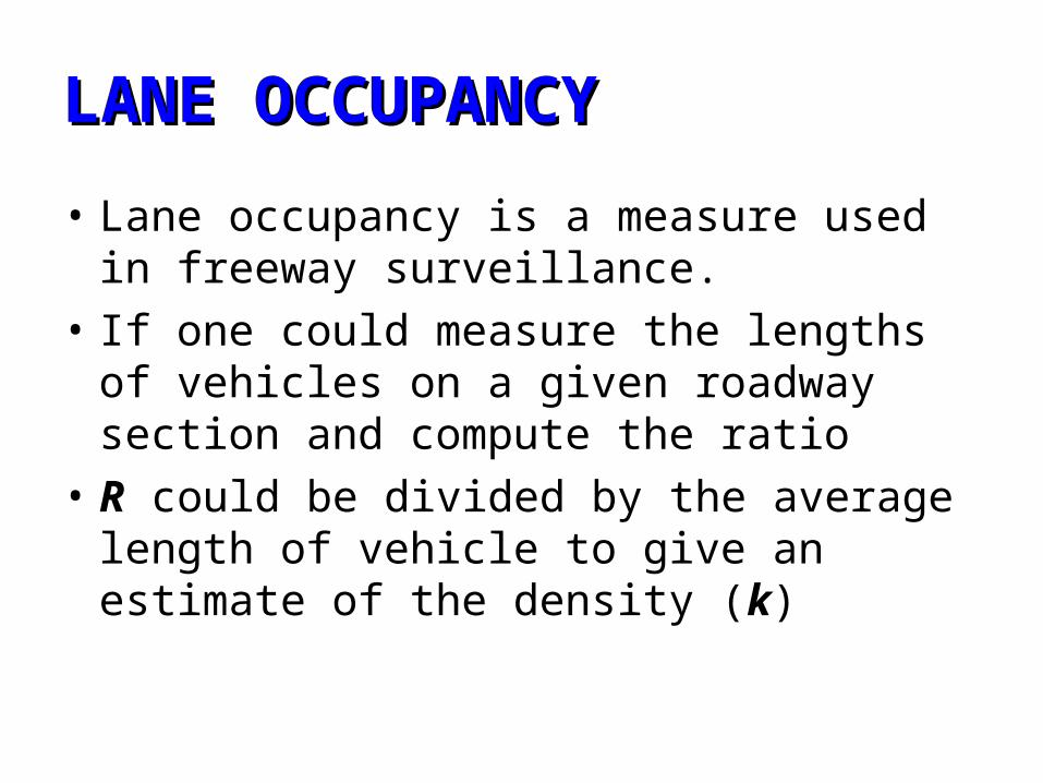
LANE OCCUPANCYLANE OCCUPANCY
• Lane occupancy is a measure used in freeway surveillance.
• If one could measure the lengths of vehicles on a given roadway section and compute the ratio
• R could be divided by the average length of vehicle to give an estimate of the density (k)
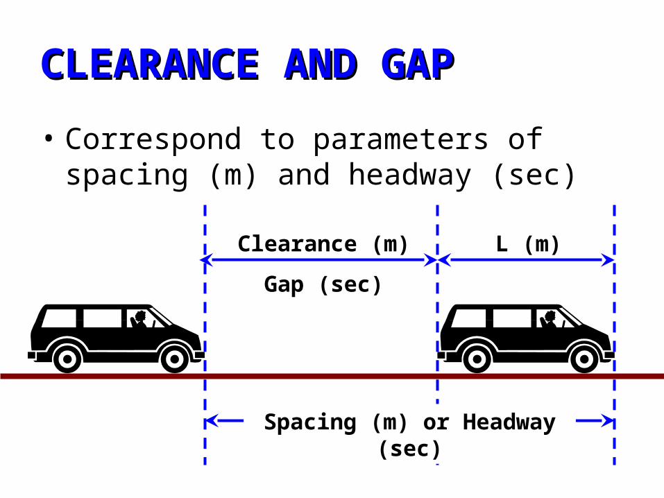
CLEARANCE AND GAPCLEARANCE AND GAP
• Correspond to parameters of spacing (m) and headway (sec)
Clearance (m)
Gap (sec)
L (m)
Spacing (m) or Headway (sec)
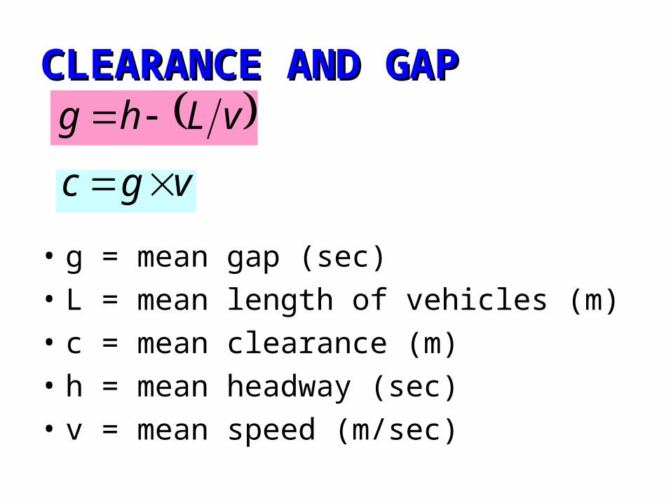
CLEARANCE AND GAPCLEARANCE AND GAP
• g = mean gap (sec)
• L = mean length of vehicles (m)
• c = mean clearance (m)
• h = mean headway (sec)
• v = mean speed (m/sec)
vLhg
vgc
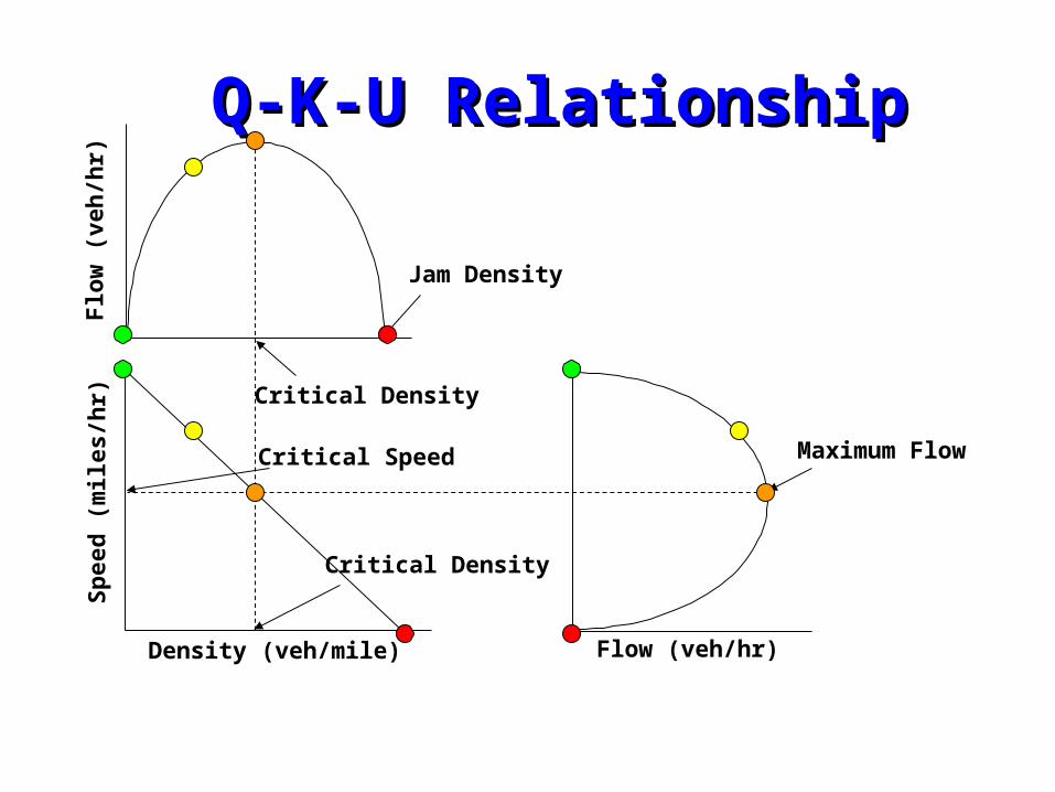
Q-K-U RelationshipQ-K-U Relationship
Maximum Flow
Flo
w (
veh
/hr)
Density (veh/mile)
Sp
eed
(m
iles/h
r)
Flow (veh/hr)
Jam Density
Critical Density
Critical Density
Critical Speed
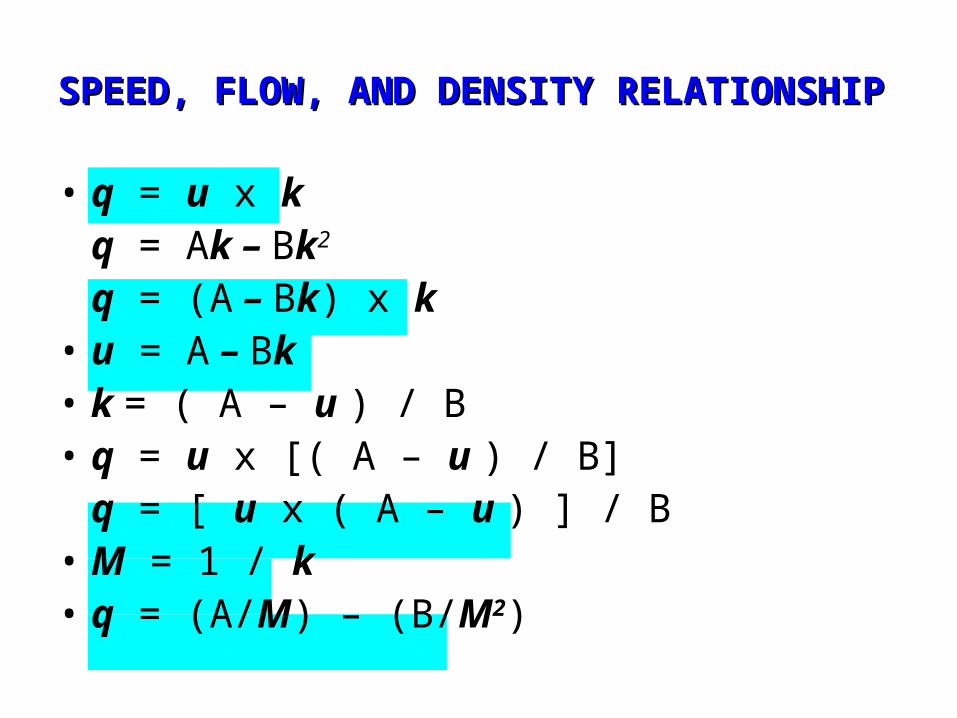
SPEED, FLOW, AND DENSITY RELATIONSHIPSPEED, FLOW, AND DENSITY RELATIONSHIP
• q = u x kq = Ak – Bk2
q = (A – Bk) x k• u = A – Bk• k = ( A – u ) / B• q = u x [( A – u ) / B]
q = [ u x ( A – u ) ] / B• M = 1 / k• q = (A/M) – (B/M2)
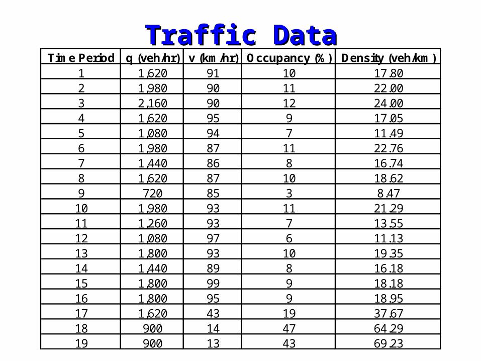
Traffic DataTraffic DataTime Period q (veh/hr) v (km/hr) Occupancy (%) Density (veh/km)
1 1,620 91 10 17.802 1,980 90 11 22.003 2,160 90 12 24.004 1,620 95 9 17.055 1,080 94 7 11.496 1,980 87 11 22.767 1,440 86 8 16.748 1,620 87 10 18.629 720 85 3 8.47
10 1,980 93 11 21.2911 1,260 93 7 13.5512 1,080 97 6 11.1313 1,800 93 10 19.3514 1,440 89 8 16.1815 1,800 99 9 18.1816 1,800 95 9 18.9517 1,620 43 19 37.6718 900 14 47 64.2919 900 13 43 69.23
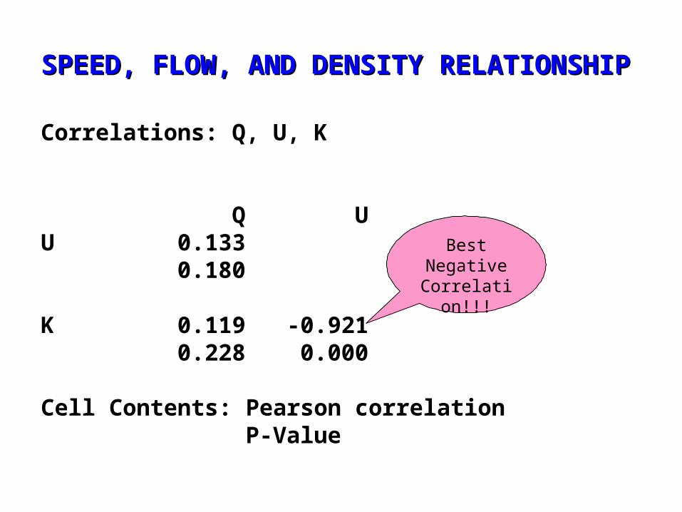
SPEED, FLOW, AND DENSITY RELATIONSHIPSPEED, FLOW, AND DENSITY RELATIONSHIP
Correlations: Q, U, K
Q UU 0.133 0.180
K 0.119 -0.921 0.228 0.000
Cell Contents: Pearson correlation P-Value
BestNegative
Correlation!!!
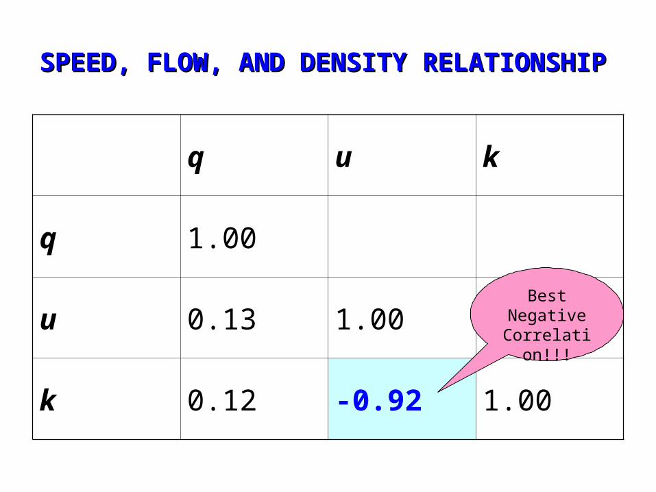
SPEED, FLOW, AND DENSITY RELATIONSHIPSPEED, FLOW, AND DENSITY RELATIONSHIP
q u k
q 1.00
u 0.13 1.00
k 0.12 -0.92 1.00
BestNegative
Correlation!!!
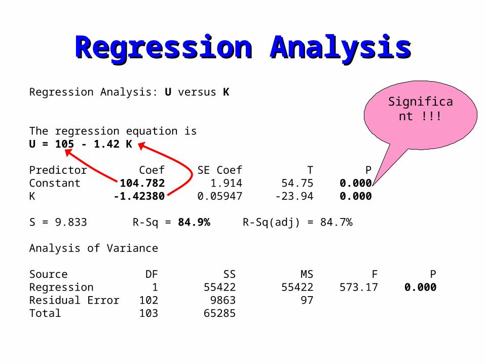
Regression AnalysisRegression AnalysisRegression Analysis: U versus K
The regression equation isU = 105 - 1.42 K
Predictor Coef SE Coef T PConstant 104.782 1.914 54.75 0.000K -1.42380 0.05947 -23.94 0.000
S = 9.833 R-Sq = 84.9% R-Sq(adj) = 84.7%
Analysis of Variance
Source DF SS MS F PRegression 1 55422 55422 573.17 0.000Residual Error 102 9863 97Total 103 65285
Significant !!!
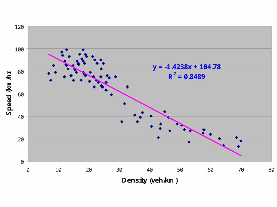
y = -1.4238x + 104.78
R2 = 0.8489
0
20
40
60
80
100
120
0 10 20 30 40 50 60 70 80
Density (veh/km)
Sp
eed
(km
/hr
SPEED, FLOW, AND DENSITY RELATIONSHIPSPEED, FLOW, AND DENSITY RELATIONSHIP
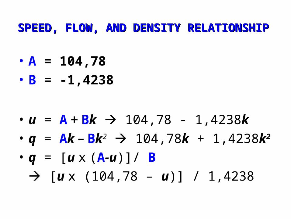
• A = 104,78
• B = -1,4238
• u = A + Bk 104,78 - 1,4238k
• q = Ak – Bk2 104,78k + 1,4238k2
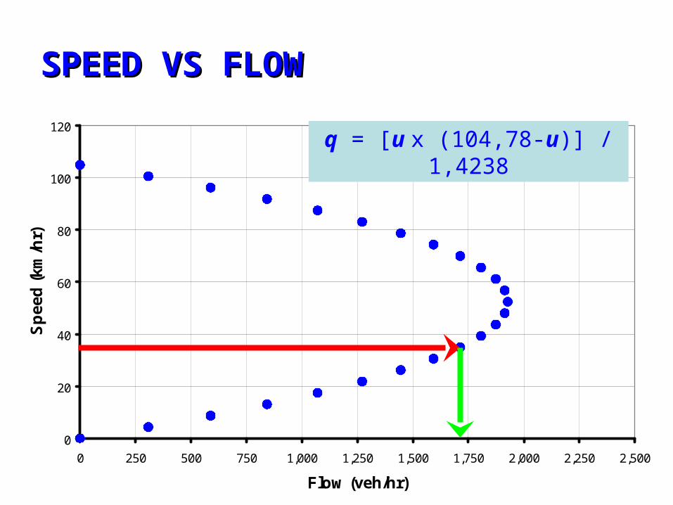
• q = [u x (A-u)]/ B
[u x (104,78 – u)] / 1,4238
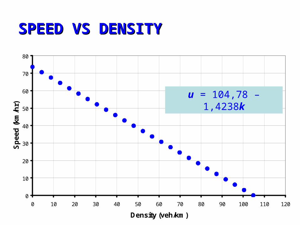
SPEED VS DENSITYSPEED VS DENSITY
0
10
20
30
40
50
60
70
80
0 10 20 30 40 50 60 70 80 90 100 110 120
Density (veh/km)
Sp
eed
(km
/hr) u = 104,78 – 1,4238k
0
500
1,000
1,500
2,000
2,500
0 10 20 30 40 50 60 70 80
Density (veh/km)
Flo
w (
veh
/km
)
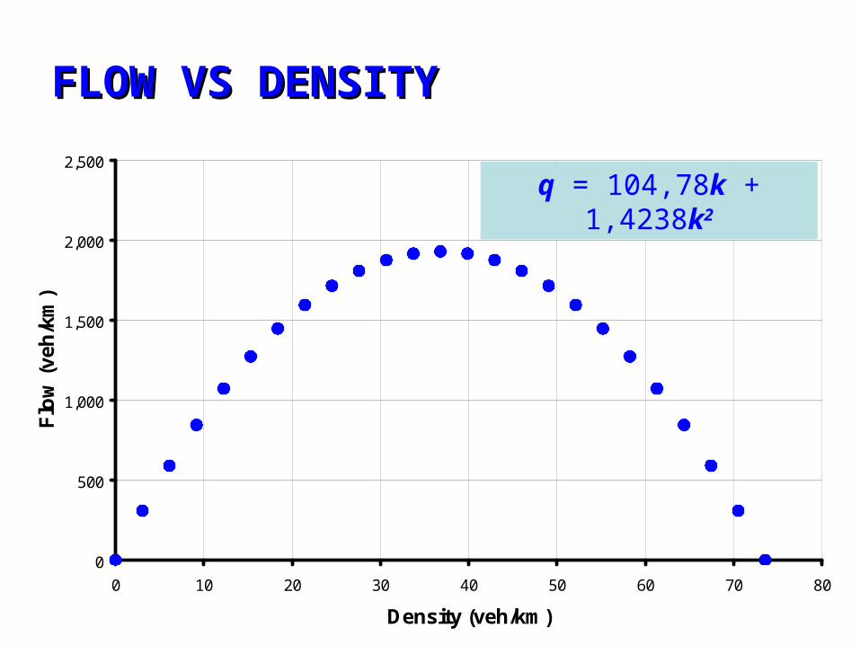
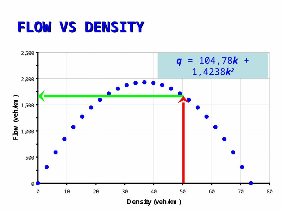
FLOW VS DENSITYFLOW VS DENSITY
q = 104,78k + 1,4238k2
0
20
40
60
80
100
120
0 250 500 750 1,000 1,250 1,500 1,750 2,000 2,250 2,500
Flow (veh/hr)
Sp
eed
(km
/hr)
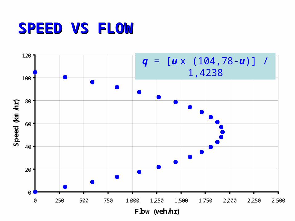
SPEED VS FLOWSPEED VS FLOW
q = [u x (104,78-u)] / 1,4238
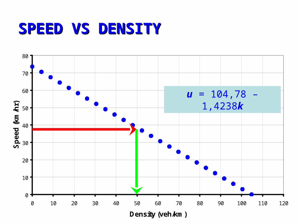
SPEED VS DENSITYSPEED VS DENSITY
0
10
20
30
40
50
60
70
80
0 10 20 30 40 50 60 70 80 90 100 110 120
Density (veh/km)
Sp
eed
(km
/hr) u = 104,78 – 1,4238k
0
500
1,000
1,500
2,000
2,500
0 10 20 30 40 50 60 70 80
Density (veh/km)
Flo
w (
veh
/km
)
FLOW VS DENSITYFLOW VS DENSITY
q = 104,78k + 1,4238k2
0
20
40
60
80
100
120
0 250 500 750 1,000 1,250 1,500 1,750 2,000 2,250 2,500
Flow (veh/hr)
Sp
eed
(km
/hr)
SPEED VS FLOWSPEED VS FLOW
q = [u x (104,78-u)] / 1,4238
Referensi :
Traffic Engineering, Roger P. Roess, Chapter 5
Fundamentals of Transportation Engineering A Multimodal Systems Approach, Jon D, Fricker, Chapter 2
Transportation Engineering An Introduction, C. Jotin Khisty, Chapter 5
Related Documents


![STAS 4273 (1983) [G52].pdf](https://static.cupdf.com/doc/110x72/577c7f1f1a28abe054a354ae/stas-4273-1983-g52pdf.jpg)


