Trophic structure of southern marine ecosystems

MARINE ECOLOGY PROGRESS SERIESMar Ecol Prog Ser

Vol. 655: 1–27, 2020https://doi.org/10.3354/meps13524

Published November 26

1. INTRODUCTION

Marine ecosystems are being profoundly trans-formed by humans affecting the integrity and sta-bility of subpolar and polar ecosystems with long-lasting consequences (Hoegh-Guldberg & Bruno 2010,

© The authors 2020. Open Access under Creative Commons byAttribution Licence. Use, distribution and reproduction are un -restricted. Authors and original publication must be credited.

Publisher: Inter-Research · www.int-res.com

*Corresponding author: [email protected]

FEATURE ARTICLE

Trophic structure of southern marine ecosystems: acomparative isotopic analysis from the Beagle

Channel to the oceanic Burdwood Bank area undera wasp-waist assumption

Luciana Riccialdelli1,*, Yamila A. Becker1, Nicolás E. Fioramonti1, Mónica Torres1, Daniel O. Bruno1,2, Andrea Raya Rey1,2,3, Daniel A. Fernández1,2

1Centro Austral de Investigaciones Científicas (CADIC), Consejo Nacional de Investigaciones Científicas y Técnicas (CONICET), Bernardo A. Houssay 200, V9410CAB Ushuaia, Tierra del Fuego, Argentina

2Instituto de Ciencias Polares, Ambiente y Recursos Naturales (ICPA), Universidad Nacional de Tierra del Fuego (UNTDF), Fuegia Basket 251, V9410CAB Ushuaia, Tierra del Fuego, Argentina

3Wildlife Conservation Society (WCS), Representación Argentina, Amenabar 1595, C1526AKC Buenos Aires, Argentina

ABSTRACT: Understanding the structure and func-tioning of marine ecosystems has become a critical issueto assess the potential short- and long-term effects ofnatural and anthropogenic impacts and to determinethe knowledge needed to conduct appropriate conser-vation actions. This goal can be achieved in part byacquiring more detailed food web information and eval-uating the processes that shape food web structure anddynamics. Our main objective was to identify large-scale patterns in the organization of pelagic food websthat can be linked to a wasp-waist (WW) structure, pro-posed for the southwestern South Atlantic Ocean. Weevaluated 3 sub-Antarctic marine areas in a regionalcontext: the Beagle Channel (BC), the Atlantic coast ofTierra del Fuego (CA) and the oceanic Burdwood Bankarea (BB). We used carbon and nitrogen isotopic infor-mation of all functional trophic groups, ranging fromprimary producers to top predators, and analyzed themthrough stable isotope-based Bayesian analyses. Wefound that BC and BB have a more pronounced WWstructure compared to CA. We identified species at midto low trophic positions that play a key role in thetrophodynamics of each marine area (e.g. Fuegian spratSprattus fuegensis, longtail southern cod Pata go no -tothen ramsayi and squat lobster Munida gregaria) andconsidered them as the most plausible WW species.The identification of the most influential species withinfood webs has become a crucial task for conservationpurposes in local and regional contexts to maintain eco -system integrity and the supply of ecosystem servicesfor the southwestern South Atlantic Ocean.

OPENPEN ACCESSCCESS

The Southwestern Atlantic Ocean has a large number ofspecies linked by an intermediate trophic level with a fewbiological components of ecological importance.

Image: Luciana Riccialdelli

KEY WORDS: Pelagic food web · Wasp-waist structure ·δ13C · δ15N · MPA Namuncurá−Burdwood Bank · Beagle Channel · Tierra del Fuego

https://crossmark.crossref.org/dialog/?doi=10.3354/meps13524&domain=pdf&date_stamp=2020-11-26

Mar Ecol Prog Ser 655: 1–27, 20202

Widdicombe & Somerfield 2012, Constable et al.2014). Anthropogenic and climate-induced impactsare known to affect individual species (e.g. by modi-fying their distributions and abundances), but theycan also change the connections that each specieshas with its prey and predators (e.g. species trophicinteractions; Constable et al. 2014, Lynam et al.2017).

Food-web organization can be described by thesetrophic interactions and the energy flows betweenspecies in a community, and thus is considered anexcellent tool to represent ecosystem complexity(Thompson et al. 2012, Young et al. 2015). The prop-agation of any impact throughout the food webwould depend, though only in part, on the type ofprocesses that shape its structure and dynamics(Young et al. 2015), since the dynamic process oftrophic interactions, or trophodynamics, is not theonly source of ecosystem regulation and structuring(Hunt & McKinnell 2006). Therefore, the propagationof such impacts will show differences if the food webis controlled by predators (i.e. top-down control), byresources (i.e. bottom-up control) or by dominantmid-trophic level species (i.e. wasp-waist control)(Cury et al. 2003, Lynam et al. 2017).

Generally, oceanic food webs are thought to be con-strained by resource availability, or bottom-up control,whereby the productivity and abundance of popula-tions at any trophic level positively correlate with andare limited by food supply (e.g. controlled by the pro-ductivity and abundance or biomass of populations atlower trophic levels) (Cury et al. 2003, Madigan et al.2012). However, due to their size, mobility and ener-getic requirements, top predators, such as marinemammals, also have important effects on the ecosys-tems where they live and feed, by regulating popula-tions of their prey (e.g. Reisinger et al. 2011). Theabundance or biomass of lower trophic levels there-fore also depends on effects from consumers abovethem (top-down control, Cury et al. 2003).

In upwelling regions and many other productivemarine areas, so-called ‘wasp-waist’ (WW) controlhas been proposed as an alternative model. Thesesystems are regulated primarily by small pelagic for-age fish (e.g. sardines) or other low to mid-trophiclevel pelagic species (e.g. crustaceans) or ‘WW spe-cies’. A low diversity, but high abundance, of thesespecies could exert top-down control of lower levels(e.g. primary producers) and bottom-up control ofmeso- and top-predators (e.g. seabirds and marinemammals), thereby regulating the energy transferbetween these trophic levels (Cury et al. 2000, Bakun2006). Food webs with a WW structure are consid-

ered to be more vulnerable to collapse, if the abun-dances of WW species decline for any reason (e.g. cli-mate change, fisheries), because of the critical ener-getic links they have with the rest of the food web(Cury et al. 2003). Despite the importance of the WWlevel with respect to energy transfer to the uppertrophic levels, recent isotope studies have suggestedthat WW systems could be more complex than previ-ously assumed, offering predators alternative foodsupply pathways (e.g. Madigan et al. 2012, Cardonaet al. 2015). Undoubtedly, trophic structure anddynamics of food webs are more complex than wethought, and multiple types of control can be operat-ing at different spatial and temporal scales with com-plex interactions under the effect of different stres-sors (Hunt & McKinnell 2006, Reisinger et al. 2011,Lynam et al. 2017).

The southwestern South Atlantic Ocean, a marineecosystem influenced by the Malvinas Current, hasbeen proposed to be under WW control (e.g.Padovani et al. 2012, Arkhipkin & Laptikhovsky2013, Saporiti et al. 2015). As in other WW systems,this region has a particular community structure,with a diverse pool of species at the lowest and at thehighest trophic levels. This large number of speciesis linked by an intermediate trophic level with only afew biological components of ecological importance,which play a key role in the structure and function-ing of this large marine ecosystem. Crustaceans (i.e.the amphipod Themisto gaudichaudii and the squatlobster Munida gregaria) and fish (i.e. Fuegian spratSprattus fuegensis and longtail southern cod Pata -gonotothen ramsayi) have been proposed as WWspecies in previous studies (e.g. Padovani et al. 2012,Arkhipkin & Laptikhovsky 2013, Diez et al. 2018).These species fulfill several criteria to be consideredWW species, including: (1) they are species with highregional abundances (Madirolas et al. 2000, Pado -vani et al. 2012, Arkhipkin & Laptikhovsky 2013), (2)they seem to occupy low to mid-trophic positions(TPs) in food webs (Ciancio et al. 2008, Riccialdelli etal. 2010), (3) many predators feed on them (Raya Reyet al. 2007, Riccialdelli et al. 2010, 2013, Scioscia etal. 2014), and (4) the population dynamics of thesespecies appear to depend on the environment (e.g.climatic variations) (Diez et al. 2016, 2018). There isa need for better identification of WW species asan essential functional trophic group to improvefood-web models, but particularly for conservationpurposes. In addition, the southern sector of this ecosystem has been subject of the establ ishmentof Argentina’s first oceanic marine protected area(MPA), the Namuncurá−Burdwood Bank (MPAN-

Riccialdelli et al.: Trophic structure of sub-Antarctic marine areas 3

BB), created by national law no. 26 875 in 2013, andmore recently the Namuncurá−Burdwood Bank II(MPAN-BBII) and Yaganes, created by national lawno. 27 490 in 2018. These MPAs have been createdbecause the areas were considered as hotspots1 (Fal-abella 2017), based on conservation priorities (e.g.seabed biodiversity) and because they individuallyor in networks contribute to protect and strengthenthe functioning of this southern region to maintainglobal ocean health. To assess the potential short-and long-term effects of environmental and anthro-pogenic impacts and conduct appropriate conserva-tion actions in those marine areas, it is critical tounderstand their structure and functioning.

This goal can be achieved by acquiring moredetailed food-web information (Young et al. 2015).Stable isotope analyses (e.g. carbon, δ13C; and nitro-gen, δ15N) have the potential to distinguish the ori-gins of organic matter in a community and trackthem across consumers (Wada et al. 1991). Therefore,by providing information on energy flow and trophicrelationships, isotopic studies allow the constructionof general food-web models (e.g. Abrantes et al.2014, Riccialdelli et al. 2017a). Moreover, since base-line δ13C and δ15N values (e.g. phytoplankton andzooplankton) can change between and within oceanbasins, isotopic differences between consumers havealso been linked to foraging habitats in space andtime (e.g. Graham et al. 2010). By providing informa-tion about different aspects of species’ trophicniches, for example through the use of Bayesian mix-ing models (Parnell et al. 2010, Jackson et al. 2011), itis possible to identify food-web connections andexplore the trophic diversity or specialization andpossible niche partitioning between species within acommunity. Moreover, community-wide trophic met-rics, as proposed by Layman et al. (2007) and devel-oped under a Bayesian approach by Jackson et al.(2011), help evaluate food-web interactions and pro-vide insight into the vertical and basal trophic struc-ture and the overall trophic diversity of the communi-ties (e.g. Abrantes et al. 2014, Demopoulos et al.2017). The application of this approach allows com-

parisons across marine areas for overall patterns infood-web structure (Saporiti et al. 2015) and to studythe effects of different impacts on such communitymetrics (e.g. Layman et al. 2007).

Our goal was to compare the main components ofthe pelagic food web of 3 sub-Antarctic marine areasin the southwestern South Atlantic Ocean: the BeagleChannel (BC), the Atlantic coast of Tierra del Fuego(CA, based on 'Costa Atlántica') and the oceanic Bur-dwood Bank (BB) area. We focused specifically onthe BB, as it is a little-known oceanic area recently de-clared an MPA (MPAN-BB and MPAN-BBII). There-fore, the study of this area is relevant in the context ofits management policies. We hypothesized that theBB has the same trophic structure (WW) proposed forits adjacent marine areas. In this regard, we proposed:(1) to identify differences and similarities between ar-eas and check if there is a pattern that could corrobo-rate our hypo thesis of the presence of WW species in aregional context, and (2) to identify these WW specieswithin each marine area.

Based on the hypothesis that a WW structurewould dominate regionally, we expected: (1) a shortvertical structure. In WW systems, the species thatoccupy the mid- to low TPs are a major food supplyfor predators, thus a short food web is expected(Cury et al. 2000); (2) a low trophic diversity and ahigh trophic redundancy for those marine areas witha more pronounced WW structure. This means a highinterspecific overlap in trophic niches, which is anexpected outcome in WW systems since a large pro-portion of species would show similar trophic habits(e.g. feeding on the same prey); (3) the presence offew WW species for each marine area with similarbut not identical trophic niches. WW species usuallydiffer in several aspects of their ecological niche (e.g.TP and general habits); thus, their influence on thetrophic web is expected to be different (Bakun 2006).

2. MATERIALS AND METHODS

2.1. Study site

The study site covers the sub-Antarctic zone at thesouthwestern portion of the South Atlantic Ocean,next to the Tierra del Fuego Archipelago, from ~52°to 56° S and from ~57° to 69° W (Fig. 1). We compared3 different marine areas: (1) the BC, including themarine zone at the southeastern tip of Tierra delFuego; (2) the CA, including the northern part ofStaten Island; and (3) the BB, including the plateauand its adjacent slope break.

1The term ‘hotspot’ in pelagic marine ecosystems is not re-stricted only to areas of high biodiversity and endemism; ithas also been used for areas of low biodiversity, but withhigh abundances, or areas of high primary productivity andhigh energy transfers (Young et al. 2015). Here, we defineda hotspot by a combination of factors including the conser-vation priorities established by Argentine law, oceano -graphic features (e.g. seamounts, shelf break), highly dy-namic (in space and time) oceanographic conditions and high biodiversity


The region is influenced by the Malvinas Current,which originates from the Antarctic CircumpolarCurrent, the Cape Horn Current that gets into thearea around the southern tip of Tierra del Fuego,freshwater discharges from Tierra del Fuego, and theStrait of Magellan and its strong tidal currents (Piola& Rivas 1997). The CA area is affected by a seasonalbut persistent front, the Magellan Front, related tothe influx of freshwater (of low salinity <32) from thePacific to the Atlantic via the Strait of Magellan andfrom the Cape Horn Current (with slightly saltierwaters <33.9) (Acha et al. 2004, Belkin et al. 2009).BB is particularly affected by both branches of theMalvinas Current that flow around the bank, causingmore oceanic and polar conditions where surfacewater temperatures range from ~5°C (autumn) to 6°C(spring), with salinities of ~34 (García Alonso et al.2018). The BB is an undersea plateau found at 50−200 m depth and surrounded by deep channels(>1000 m depth). It is located about 150 km east ofStaten Island and 200 km south of the Falkland/Malvinas Islands. The BB is also the site where Ar -gentina established the open-sea MPAN-BB (Fala-bella 2017) and the MPAN-BBII (at the present time,both MPAs are under a unification process).

Lastly, within this region, the BC is a particularmarine environment that can be as much as 30 kmwide at its eastern mouth and extends nearly 200 kmto the west, connecting the Pacific and the AtlanticOceans (Isla et al. 1999). Pushed by the preponder-

ance of west and southwesterly winds, the dilutedwaters of the BC, originating from high precipitationand glacial melting, flow towards the Atlantic(Balestrini et al. 1998). Surface water temperaturesrange from ~4°C in winter to ~9°C in summer, andsalinity ranges from 27 to 31 from the inner part ofthe BC to the eastern mouth (Balestrini et al. 1998).The third MPA, Yaganes, is located at the southeastsection of the BC and south of Staten Island from the500 m isobaths towards the polar front.

2.2. Sample collection and processing

We conducted most of the biological sampling (or -ganic matter in sediments, primary producers andconsumers) during 3 research cruises at the end ofthe austral summer and autumn (February−April) in2014, 2015 and 2016, onboard the RV ‘Puerto De -seado’ (cruises BOPDMar2014 and BOPDApr2016), avessel belonging to the Argentine National Scientificand Technical Research Council (CONICET); the‘SB-15 Tango’ (TANGOFeb2015), a vessel belongingto the Argentine Coastguard (Prefectura Naval); andonboard small vessels (i.e. zodiacs) belonging to theAustral Center for Scientific Research (CADIC-CON-ICET). We increased samples for specific and impor-tant species (e.g. Sprattus fuegensis) that could becollected onboard the RV ‘Victor Angelescu’, a vesselbelonging to the Argentine National Institute for

Fig. 1. Marine areas studied: Beagle Channel, Atlantic coast of Tierra del Fuego, and Burdwood Bank, including the MarineProtected Areas of Argentina Namuncurá − Burdwood Bank I (red line: core area, green line: buffer area, black line: transitionarea), Burdwood Bank II and Yaganes. Solid and dashed lines are used for illustrative purposes to distinguish thecurrents/fronts. Sampling stations are indicated, where open circles: BODPMar2014 survey, black circles: TANGOFeb2015survey, gray circles: BOPDApr2016 survey, black cross: VA1418 survey. CHC: Cape Horn Current; MC: Malvinas Current:

MF: Magellan Front, UpA: upwelling areas


Fisheries Research (INIDEP), during an oceano-graphic research cruise in November 2018 (VA1418).

We sampled marine mammals through strandedanimals found on beach surveys along the north-eastern and southern coast of Tierra del Fuego (L.Riccialdelli on-going long-term studies under the In -vestigaciones en Mamíferos Marinos Australes [IMMA]Project), and seabirds were sampled in their breed-ing colonies from the BC (Martillo and BridgesIslands) and Staten Island (A. Raya Rey on-goinglong-term studies). To complement our fieldwork, wealso used isotopic data of specific species and alsofrom basal sources (e.g. sediment particulate organicmatter [SPOM], benthic baselines) that were previ-ously published (e.g. Saporiti et al. 2014, Riccialdelliet al. 2017a, Bas et al. 2019, 2020) or unpublisheddata available for the region.

2.2.1. Primary producers

We collected phytoplankton samples at 37 sam-pling stations distributed in the 3 marine areas witha 25 μm net during vertical trawling from 20 mdepth. We pre-filtered each sample onboard with a115 μm mesh (to remove organisms >115 μm) andthen filtered samples onto pre-combusted (450°Cfor 4 h) GF/F type fiber filters of 0.7 μm nominalpore size. Filters with phytoplankton were keptfrozen (−20°C) until drying at 60°C for 48 h. Wecollected macroalgae at 25 sampling stations in BCand 7 in CA by hand during coastal surveys andonboard small boats (zodiacs) from CADIC-CON-ICET. We cleaned the fronds of macroalgae byrinsing them with distilled (DI) water and cleanedthem of epibionts and debris.

2.2.2. Consumers

We collected zooplankton at 40 sampling stationswith a 200 μm net during 5 min of oblique trawlingfrom 100 m depth to the surface water, and keptfrozen (−20°C) onboard until processing. In the labo-ratory, we separated zooplankton samples into taxo-nomical groups (e.g. euphausiids, copepods, amphi -pods), using a Leica stereoscope. We collectedinvertebrates (e.g. crustaceans, mollusks) and fishspecies at 19 sampling stations (BC = 5, CA = 6 and BB= 8) during 10 min of bottom trawling. We only sam-pled muscle from these organisms, but when the indi-vidual was too small, we pooled the entire organism(e.g. zooplankton groups, small crustaceans).

2.2.3. Predators

Among the pool of samples that we had availablefor top predators, and based on previous knowledgefrom the literature and our personal observations,we chose only a few species that we consideredrepresentative of each marine area. We collectedskin and muscle samples from only fresh andrecently stranded (<24 h) marine mammals, sincedecomposition is not a significant source of isotopevariation within that time (Payo-Payo et al. 2013).Samples were frozen (−20°C) until processing. Toavoid the effects on δ13C values associated with thepresence of lipids, we performed a lipid extractionwith a 2:1 chloroform:methanol solution. While thisextraction does not significantly alter skin δ15N val-ues (Newsome et al. 2018), we also analyzed thesame samples without treatment to assure unbiasedδ15N values. We collected and cleaned feathers andblood samples from seabirds following Raya Reyet al. (2012). All samples (macroalgae to top con-sumers) were lyophilized (48 h), ground and mixed(homogenized).

2.2.4. SPOM

We collected samples from surface sediments withdredges at 18 sampling stations during the BOP-DApr2016 survey cruise and kept them frozen(−20°C) onboard in plastic bags. The sediment con-tains organic and inorganic C in the form of carbon-ates. Since carbonates may be enriched in 13C com-pared to organic C, it is necessary to remove thecarbonates from the sediment to avoid their influ-ence. Thus, we divided each sample in 2 andremoved most of the carbonates in the first HCl fumi-gation, following Harris et al. (2001). During thistreatment, we placed ~40 mg of dried sediment (pre-viously oven-dried at 60°C for 48 h) in Eppendorftubes and added DI water (~75 μl) to moisten the sed-iment. Later, we exposed these samples to HCl (12N)vapor for 12 h in a closed glass desiccator cabinet.After acid fumigation, we again dried each sample at60°C for 4 h. We used the second half of the sample(untreated) to obtain an estimation of δ15N.

2.3. Stable isotope analysis

We weighed an aliquot (0.6 to 3.0 mg, dependingon the sample type) of dried sample into tin capsulesfor δ13C and δ15N analysis. We analyzed samples


from BOPDMar2014 and TANGOFeb2015 oceano-graphic surveys and samples of top predators with aThermo DELTA V Advantage isotope-ratio massspectrometer at the Institute of Geochronology andIsotopic Geology (Instituto de Geocronología yGeología Isotópica, INGEIS, UBA-CONICET). Weanalyzed samples from BOPDApr2016 and VA1418oceanographic surveys with a Thermo ScientificDELTA V Advantage isotope-ratio mass spectrome-ter at the Environmental Sciences Stable IsotopeLaboratory (Laboratorio de Isótopos Estables enCiencias Ambientales, LIECA, IANIGLA-CONICET).In general, we analyzed 1 sample per collected indi-vidual (or pooled individuals), but to have a bettercharacterization of the basal resources (phytoplank-ton), we carried out double analyses in samples withsufficient material. We expressed isotope results indelta (δ) notation; units are expressed as ‰, using theequation:

δ13C or δ15N = [(Rsample/Rstandard) − 1] × 1000 (1)

where Rsample and Rstandard are the 13C/12C or 15N/14Nratios of the sample and standard, respectively. Thestandards were Vienna Pee Dee Belemnite limestonefor carbon and air (atmospheric N2) for nitrogen(Gonfiantini 1978, Coplen et al. 1992). All isotopemeasures are reported as mean ± SD. We were ableto quantify the analytical precision via repeatedanalysis of internal reference standards. Based on 3internal standards (caffeine, sugar and collagenTRACE), the within-run standard deviation (SD) was0.2‰ for δ13C and δ15N for samples analyzed atINGEIS. Based on 3 internal standards (caffeineIECA 17, collagen IECA17 and USGS41a) the within-run SD was 0.06‰ for δ13C and δ15N for samples ana-lyzed at LIECA. We also measured the weight per-cent carbon and nitrogen concentration of eachsample, which is reported as a [C]/[N] ratio. Since wedid not conduct lipid-extraction of our samples(except top predators) prior to isotopic analysis, wenormalized δ13C values, following Post et al. (2007),and we applied a correction factor of −0.022 yr−1 to allsample carbon isotope values to the most presentsample (2018 yr) to account for the Suess effect, orthe anthropogenic decrease in the δ13C of atmos-pheric CO2 due to the burning of fossil fuels (Franceyet al. 1999).

We sampled skin and muscle of a calf (i.e. lactat-ing) Burmeister’s porpoise Phocoena spinipinnis andminke whale (Balaenoptera sp.) and used a generaltrophic correction to approximate values of an adultof each species (see Section 2.4.2). We correctedbone collagen data with a general tissue fractiona-

tion factor of ~4‰ for δ13C to approximate muscle(Hedges et al. 2005). We divided pinniped data(Drago et al. 2009) into CA and BC individualsaccording to the location of death, based on sourcedata provided by the RNP Goodall Foundation.

2.4. Data treatment

To perform stable isotope analysis and to identifypatterns in food web structure, we selected a pool ofspecies that were the most abundant in the oceano-graphic surveys and/or have been identified asimportant species for the structure and dynamics ofeach marine area (for details, see Table 1). Wegrouped these organisms into 6 functional trophicgroups, considering a combination of ecological andtaxonomic characteristics: (1) inputs (primary pro-ducers and SPOM), (2) zooplankton (copepods,euphausiids and amphipods), (3) pelagic fish andcrustaceans, (4) benthopelagic species (crustaceans,fish and squids), (5) demersal species (fish) and (6)top predators (seabirds and marine mammals).

2.4.1. Trophic structure: community-wide metricsand isotopic niche estimation

We described the trophic structure of each commu-nity through the Bayesian approach of Layman met-rics (Layman et al. 2007, Jackson et al. 2011), usingthe Stable Isotope Bayesian Ellipses in R (SIBER)package of SIAR in R (Parnell et al. 2010, Jackson etal. 2011, R Development Core Team 2019) based onthe δ13C and δ15N values of 612 biological compo-nents for the entire region. Specifically, for eacharea, we analyzed 19 species/groups (n = 234) fromthe BC; 22 (n = 204) from CA and 21 (n = 174) fromthe BB area. We calculated the Bayesian estimate ofthe community metrics originally proposed by Lay-man et al. (2007) and comparatively analyzed themamong the 3 marine areas under study (Jackson et al.2011). The nitrogen range (NR) describes the verticalstructure (trophic length) of each community (e.g.larger range suggests more trophic levels). Nitrogenisotope ratios (15N:14N, δ15N) generally show higherincreases of ~2−5‰ between consumers and theirfood and thus, in addition to reflecting food sources,are often used as an indicator of TP and food chainlength (Post 2002). The carbon range (CR) representsthe basal structure of each community and can givean estimate of the trophic diversity at the base ofeach community with varying δ13C values. The natu-


Fu

nct

ion

al t

rop

hic

Sp

ecie

sA

bb

Nδ13

Cra

wδ13

Cn

orm

δ13C

sues

sδ15

NC

:NS

amp

ling

Ref

eren

ceg

rou

p/S

IBE

RM

ean

SD

Mea

nS

DM

ean

SD

Mea

nS

Dye

ar

Bea

gle

ch

ann

el (

BC

)G

rou

p 1

:P

hyt

opla

nk

ton

aP

hyt

o22

−20

.22.

6−

20.3

2.6

10.6

2.8

6.9

2014

/201

5T

his

stu

dy

inp

uts

M

acro

alg

ae (

Mac

rocy

stis

pyr

ifer

a)M

acro

25−

15.1

1.5

−15

.21.

58.

40.

915

.220

14T

his

stu

dy

SP

OM

SP

OM

3−

18.9

1.5

−18

.91.

5−

19.0

1.4

9.4

1.3

10.1

2010

/201

6R

icci

ald

elli

et a

l. (2

017a

), t

his

stu

dy

Gro

up

2:

Cop

epod

saC

ope

19−

21.9

2.6

−18

.92.

3−

19.0

2.3

9.8

2.0

6.4

2014

/201

5/20

16T

his

stu

dy

zoop

lan

kto

n

Eu

ph

ausi

idsa

Eu

ph

a4

−21

.81.

5−

20.3

1.4

−20

.41.

410

.81.

14.

820

16T

his

stu

dy

Mu

nid

a g

reg

aria

− p

elag

ica

MG

P11

−19

.72.

5−

18.0

2.6

−18

.02.

69.

90.

95.

120

14/2

015/

2016

Th

is s

tud

yT

hem

isto

gau

dic

hau

dii

aT

G4

−22

.01.

7−

20.2

1.6

−20

.21.

69.

23.

75.

120

14/2

015/

2016

Th

is s

tud

yG

rou

p 3

: pel

agic

Mu

nid

a g

reg

aria

− b

enth

icM

GB

19−

16.7

0.5

−16

.30.

4−

16.5

0.5

14.0

0.8

3.7

2009

/201

4R

icci

ald

elli

et a

l. (2

017a

), t

his

stu

dy

fish

an

dO

don

test

hes

sm

itti

Osm

itt

6−

13.9

1.0

−−

−14

.21.

015

.71.

63.

220

08L

. Ric

cial

del

li (u

np

ub

l. d

ata)

cru

stac

ean

s S

pra

ttu

s fu

egen

sis

Sfu

eg20

−17

.60.

6−

16.5

1.0

−16

.61.

013

.30.

74.

520

13/2

018

L. R

icci

ald

elli

(un

pu

bl.

dat

a), t

his

stu

dy

Gro

up

4:

Pat

agon

otot

hen

cor

nu

cola

Pco

rn3

−15

.20.

6−

14.6

0.5

−14

.70.

515

.90.

73.

920

14T

his

stu

dy

ben

thop

elag

icP

atag

onot

oth

en t

esse

llat

aP

tess

e15

−16

.91.

1−

16.4

1.0

−16

.51.

013

.72.

03.

920

09/2

014

Ric

cial

del

li et

al.

(201

7a),

th

is s

tud

ysp

ecie

sP

atag

onot

oth

en r

amsa

yiP

ram

4−

16.9

0.4

−16

.50.

2−

16.6

0.2

12.4

0.9

3.7

2014

/201

6T

his

stu

dy

Ele

gin

ops

mac

lovi

nu

sE

mac

lo20

−15

.50.

9−

15.5

0.7

−15

.70.

716

.40.

43.

420

10/2

014

Ric

cial

del

li et

al.

(201

7a),

th

is s

tud

yG

rou

p 5

: dem

er-

Cot

top

erca

tri

glo

ides

Ctr

igl

6−

16.2

0.4

−15

.90.

5−

16.0

0.4

14.3

0.3

3.6

2014

/201

6T

his

stu

dy

sal s

pec

ies

Gro

up

6:

Arc

toce

ph

alu

s au

stra

lisb

Aau

st8

−16

.91.

2−

14.6

20.6

2009

Sap

orti

ni e

t al

. (20

15),

Bas

et

al. (

2019

)to

p p

red

ator

sO

tari

a fl

aves

cen

sbO

flav

5−

13.4

0.9

−13

.81.

020

.71.

419

81 t

o 20

07D

rag

o et

al.

(200

9), B

as e

t al

. (20

19)

Ph

ocoe

na

spin

ipin

nis

cP

spin

1(2)

−14

.50.

1−

14.5

0.1

16.6

0.2

3.2

2016

Th

is s

tud

yS

eab

ird

s (S

ph

enis

cus

mag

ella

nic

us,

Sea

B38

−16

.70.

6−

16.6

0.5

−16

.60.

516

.20.

53.

520

14A

. Ray

a R

ey (

un

pu

bl.

dat

a)P

hal

acro

cora

x at

rice

ps,

Leu

cop

hae

us

scor

esb

ii)

Atl

anti

c co

ast

of

Tie

rra

del

Fu

ego

(C

A)

Gro

up

1: i

np

uts

Ph

ytop

lan

kto

na

Ph

yto

18−

16.2

2.6

−16

.22.

68.

32.

06.

520

14/2

015

Th

is s

tud

yM

acro

alg

ae (

Mac

rocy

stis

pyr

ifer

a)M

acro

7−

11.2

2.8

−11

.32.

812

.51.

08.

820

13L

. Ric

cial

del

li (u

np

ub

l. d

ata)

SP

OM

SP

OM

1−

20.6

−20

.76.

65.

420

16T

his

stu

dy

Gro

up

2:

Cop

epod

saC

ope

14−

20.7

1.9

−17

.11.

5−

17.2

1.5

7.4

1.1

7.0

2014

/201

5/20

16T

his

stu

dy

zoop

lan

kto

n

Eu

ph

ausi

idsa

Eu

ph

a4

−21

.41.

1−

20.1

1.0

−20

.11.

07.

71.

14.

620

14/2

016

Th

is s

tud

yM

un

ida

gre

gar

ia −

pel

agic

aM

GP

7−

20.9

1.0

−19

.11.

2−

19.2

1.2

8.6

0.9

5.1

2014

/201

6T

his

stu

dy

Th

emis

to g

aud

ich

aud

iiT

G7

−20

.91.

9−

18.3

1.5

−18

.31.

58.

11.

16.

020

14/2

015/

2016

Th

is s

tud

yG

rou

p 3

: pel

agic

Mu

nid

a g

reg

aria

−b

enth

ica

MG

B2

−18

.70.

0−

18.1

0.0

−18

.20.

011

.00.

03.

920

14T

his

stu

dy

fish

an

dO

don

test

hes

sm

itti

Osm

itt

5−

15.3

0.5

−15

.50.

517

.30.

13.

220

07R

icci

ald

elli

et a

l. (2

010,

201

3)cr

ust

acea

ns

Sp

ratt

us

fueg

ensi

sS

fueg

11−

21.8

2.0

−18

.11.

4−

18.2

1.4

12.1

0.7

7.0

2014

Th

is s

tud

yG

rou

p 4

:M

acru

ron

us

mag

ella

nic

us

Mm

age

5−

16.1

0.4

−16

.40.

415

.10.

33.

120

07R

icci

ald

elli

et a

l. (2

010,

201

3)b

enth

opel

agic

Pat

agon

otot

hen

ram

sayi

Pra

m19

−17

.20.

5−

17.0

0.7

−17

.10.

712

.50.

73.

520

14/2

016

Th

is s

tud

ysp

ecie

sE

leg

inop

s m

aclo

vin

us

Em

aclo

9−

13.9

2.2

−14

.12.

217

.31.

33.

120

07R

icci

ald

elli

et a

l. (2

010,

201

3)S

alil

ota

aust

rali

sS

aust

13−

16.3

1.0

−16

.51.

014

.91.

43.

420

07/2

008/

2014

Ric

cial

del

li et

al.

(201

0, 2

013)

, th

is s

tud

yS

qu

ids

(Ill

ex a

rgen

tin

us,

S

qu

id11

−17

.51.

0−

16.9

0.9

−17

.00.

912

.51.

34.

020

14T

his

stu

dy

Dor

yteu

this

gah

i)G

rou

p 5

:C

otto

per

ca t

rig

loid

esC

trig

l6

−17

.42.

8−

17.1

2.9

−17

.22.

913

.31.

43.

620

14/2

016

Th

is s

tud

yd

emer

sal

Mer

lucc

ius

aust

rali

sM

aust

14−

15.9

0.5

−16

.20.

517

.70.

73.

120

07/2

008

Ric

cial

del

li et

al.

(201

0, 2

013)

spec

ies

Mer

lucc

ius

hu

bb

siM

hu

bb

3−

16.6

0.2

−16

.90.

217

.70.

33.

220

08R

icci

ald

elli

et a

l. (2

010,

201

3)D

isso

stic

hu

s el

egin

oid

esD

eleg

1−

16.5

−16

.816

.33.

120

07L

. Ric

cial

del

li (u

np

ub

l. d

ata)

Tab

le 1

. Bio

log

ical

com

pon

ents

an

alyz

ed f

rom

th

e B

eag

le C

han

nel

, th

e A

tlan

tic

coas

t of

Tie

rra

del

Fu

ego

and

Bu

rdw

ood

Ban

k m

arin

e ar

eas.

Th

e tr

oph

ic g

rou

ps

rep

orte

d a

reth

ose

use

d t

o es

tim

ate

the

stan

dar

d e

llip

se a

reas

an

d L

aym

an m

etri

cs i

n S

IBE

R. δ

13C

val

ues

are

rep

orte

d a

s: (

1) r

aw v

alu

es w

ith

no

corr

ecti

ons

(δ13

Cra

w),

(2)

raw

val

ues

cor

-re

cted

by

lipid

nor

mal

izat

ion

(δ13

Cn

orm

) (P

ost

et a

l. 20

07)

and

(3)

raw

val

ues

cor

rect

ed b

y lip

id n

orm

aliz

atio

n a

nd

Su

ess

effe

ct (δ13

Csu

ess)

. All

top

pre

dat

or s

amp

les

wer

e lip

idex

trac

ted

. C:N

val

ues

of s

edim

ent p

arti

cula

te o

rgan

ic m

atte

r (S

PO

M) c

orre

spon

d to

aci

dif

ied

sam

ple

s. A

bb

: sp

ecie

s/g

rou

p a

bb

revi

atio

ns.

Em

pty

cel

ls: n

o d

ata


ral occurrence of 13C to 12C (expressedin δ notation as δ13C) can vary substan-tially be tween primary producers withdifferent photosynthetic pathways(e.g. C3 plants vs. C4 plants or phyto-plankton vs. macroalgae; France 1995,Peterson 1999), and exhibit a smallincrease (~0−2‰) between consumersand their food (Rau et al. 1983). There-fore, δ13C is commonly used as a sourceindicator in food-web studies. Themean distance to the centroid (CD)gives a measure of the average degreeof trophic diversity within a commu-nity. The mean nearest-neighbor dis-tance (MNND) assesses the overallsimilarity of trophic niches among spe-cies within a community, and the SD ofMNND provides a measure of theevenness of the distribution of thetrophic niches in bi-blot space (e.g.δ13C and δ15N). The convex hull area(TA) was estimated; however, it isknown that it may have large biasesdue to sample size (Jackson et al.2011). In order to overcome the limita-tion of TA, we also calculated the stan-dard ellipse area corrected for smallsample size (SEAC, expressed in ‰2).SEAC was fitted to 40% of the data torepresent isotopic niche width for eachtrophic group in a given community(Jackson et al. 2011). For statisticalcomparisons of the isotopic niche areabetween trophic groups, we calculatedthe Bayesian estimate of the standardellipse area (SEAB) using SIBER (Jack-son et al. 2011). The SEAB provides adescription of the isotopic niche of apopulation or community, and it is notaffected by bias associated with sam-ple size or number of groups (Jacksonet al. 2011), allowing us to compare the3 marine areas with a different numberof biological components.

In addition, to evaluate a potentialbias introduced by differences in theranges of δ13C and δ15N values, we alsocomputed the community metrics (di -versity metrics) in a standardized mul-tidimensional space, following Cucher-ousset & Villéger (2015) and using theequation:

Fu

nct

ion

al t

rop

hic

Sp

ecie

sA

bb

Nδ13

Cra

wδ13

Cn

orm

δ13C

sues

sδ15

NC

:NS

amp

ling

Ref

eren

ceg

rou

p/S

IBE

RM

ean

SD

Mea

nS

DM

ean

SD

Mea

nS

Dye

ar

Gro

up

6: t

opC

eph

alor

hyn

chu

s co

mm

erso

nii

Cco

mm

17−

15.1

0.5

−15

.20.

516

.50.

73.

420

09 t

o 20

13T

his

stu

dy

pre

dat

ors

Ota

ria

flav

esce

nsb

Ofl

av16

−13

.00.

6−

13.3

0.5

20.7

0.9

1981

to

2007

Dra

go

et a

l. (2

009)

Sea

bir

ds

(Sp

hen

iscu

s m

agel

lan

icu

s)S

eaB

14−

18.1

0.2

−17

.70.

2−

17.8

0.2

15.5

0.3

3.8

2014

A. R

aya

Rey

(u

np

ub

l. d

ata)

Bu

rdw

oo

d B

ank

(B

B)

Gro

up

1: i

np

uts

Ph

ytop

lan

kto

na

Ph

yto

10−

26.0

4.3

−26

.14.

33.

80.

47.

720

15T

his

stu

dy

SP

OM

SP

OM

16−

24.9

0.9

−24

.90.

9−

24.9

0.9

5.2

1.1

6.4

2016

Th

is s

tud

yG

rou

p 2

:C

opep

odsa

Cop

e20

−26

.61.

7−

22.2

2.1

−22

.42.

23.

60.

97.

820

15/2

016

Th

is s

tud

yzo

opla

nk

ton

E

up

hau

siid

saE

up

ha

22−

24.9

1.3

−23

.51.

5−

23.6

1.5

5.6

1.3

4.8

2015

/201

6T

his

stu

dy

Mu

nid

a g

reg

aria

−p

elag

ica

MG

P1

−25

.0−

22.2

7.4

6.2

2016

Th

is s

tud

yT

hem

isto

gau

dic

hau

dii

aT

G21

−25

.41.

2−

23.1

1.7

−23

.11.

75.

51.

15.

720

15/2

016

Th

is s

tud

yG

rou

p 3

: pel

agic

Mu

nid

a sp

inos

aM

spin

7−

20.6

0.5

−19

.70.

4−

19.8

0.4

8.6

0.3

4.2

2016

Th

is s

tud

yfi

sh a

nd

Sp

ratt

us

fueg

ensi

sS

fueg

5−

20.8

0.1

−20

.70.

2−

20.7

0.2

9.1

0.1

3.4

2018

Th

is s

tud

ycr

ust

acea

ns

Gro

up

4:

Mac

ruro

nu

s m

agel

lan

icu

sM

mag

e2

−18

.01.

5−

18.1

1.5

13.8

0.1

2009

/201

0Q

uill

feld

t et

al.

(201

5)b

enth

opel

agic

Pat

agon

otot

hen

ele

gan

sP

ele

3−

21.1

2.9

−21

.22.

8−

21.3

2.8

11.9

1.5

3.3

2016

Th

is s

tud

ysp

ecie

sP

atag

onot

oth

en r

amsa

yiP

ram

12−

21.3

1.2

−21

.31.

2−

21.3

1.2

9.5

1.4

3.3

2016

Th

is s

tud

yS

alil

ota

aust

rali

sS

aust

1−

19.9

−20

.410

.32.

820

16T

his

stu

dy

Sem

iros

sia

ten

era

Ste

n1

−21

.7−

21.5

11.3

3.6

2016

Th

is s

tud

yS

qu

id−

ocea

nic

(G

onat

us

anta

rcti

cus,

Sq

uid

4−

22.0

0.6

−22

.00.

69.

52.

23.

2A

lvit

o et

al.

(201

5)K

ond

akov

ia l

ong

iman

a)G

rou

p 5

:C

otto

per

ca t

rig

loid

esC

trig

l10

−21

.82.

6−

21.9

2.5

−22

.02.

512

.11.

23.

220

16T

his

stu

dy

dem

ersa

l sp

ecie

sD

isso

stic

hu

s el

egin

oid

esD

eleg

4−

22.3

1.8

−21

.90.

4−

21.5

0.9

11.8

1.3

4.2

2016

Th

is s

tud

yG

rou

p 6

: top

Glo

bic

eph

ala

mel

as e

dw

ard

iiG

mel

as6

−16

.60.

6−

16.7

0.6

15.9

1.5

3.6

2015

Th

is s

tud

yp

red

ator

s L

agen

orh

ynch

us

cru

cig

erb

Lcr

uc

7−

21.3

0.9

−21

.81.

110

.20.

63.

019

77 t

o 20

11R

icci

ald

elli

et a

l. (2

010,

un

pu

bl.

dat

a)B

alae

nop

tera

sp

.cM

ink

e3

−24

.71.

0−

24.7

1.0

5.3

0.2

3.2

2016

Th

is s

tud

yS

eab

ird

s (E

ud

ypte

s ch

ryso

com

e)S

eaB

18−

22.6

0.7

−22

.20.

7−

22.3

0.7

10.6

0.5

3.8

2014

A. R

aya

Rey

(u

np

ub

l. d

ata)

Zip

hiu

s ca

viro

stri

sZ

cavi

1−

17.4

−17

.413

.83.

220

14T

his

stu

dy

a Poo

led

ind

ivid

ual

s in

eac

h s

amp

le; b

Sam

ple

s b

ased

on

bon

e co

llag

en; c C

alf

Tab

le 1

(co

nti

nu

ed)


δkst = (δk − min(δk)) / (max(δk) − min(δk)) (2)

where δkst is the standardized value of each stableisotope (δk) that is scaled to have the same range(0−1). With respect to basal and vertical structure, wesaw no need to standardize these values, since thecomparison between these measures between com-munities is independent of each other, and in fact,these differences are accounted for when calculatingand comparing these metrics between communities(Cucherousset & Villéger 2015).

2.4.2. WW species

To identify possible groups of WW species for eachmarine area and analyze their importance in thetrophic dynamics of each community, we:

(1) performed a cluster analysis for each commu-nity based on δ13C and δ15N values of each species.To create each cluster, we used the complete linkagemethod and Euclidean distances;

(2) estimated the relative TP of each species/groupwithin each functional trophic group, respectively,using 2 different models:

Model 1: TP was estimated using the equation pro-posed by Post (2002):

TPi = [(δ15Ni − (α × δ15Nb1 + (1 − α)× δ15Nb2))/TDF] + TPb

(3)

where TPi is the TP of each consumer i (individual/species/ group) considered, and δ15Ni is the nitrogenisotope composition of each consumer i. This modelconsidered 2 baselines, thus δ15Nb1 and δ15Nb2 are themean nitrogen isotope composition of baseline 1(pelagic) and 2 (benthic), and TPb represents the TPof both baselines in each marine area. TDF is the troph -ic discrimination factor for nitrogen values (TDF =Δ15N). To solve this equation, α is calculated as thecontribution of baseline 1 to the diet of the consumerwith a mixing model based on carbon and consider-ing the isotopic fractionation of carbon (Δ13C):

α = (δ13Ci − δ13Cb2 + Δ13C / (δ13Cb1 − δ13Cb2) (4)

where δ13Ci, δ13Cb1 and δ13Cb2 are the mean nitro-gen carbon isotope composition of each consumer,baseline 1 (pelagic) and baseline 2 (benthic), re -spectively.

Model 2: we performed a Bayesian estimation ofTP, using the full model of ‘tRophic Position’ in R(Quezada-Romegialli et al. 2018) that accounts forthe same data as Model 1, but calculates TPs in aBayesian framework.

We used as baselines the isotope composition of pri-mary consumers since it integrates seasonal and spa-tial variation in the stable isotope composition of pro-ducers (Cabana & Rasmussen 1996). Pelagic primaryconsumers were considered as baseline 1 (b1), andwe used the δ15N and δ13C values of mixed zooplank-ton (copepods+euphausiids) of each marine area toincorporate the entire isotopic variability at the base(mean values in Table 1). Benthic primary consumerswere considered as baseline 2 (b2). We used the δ15Nand previously published δ13C values (mean ± SD) ofNacella magellanica for CA (δ15N = 11.9 ± 0.3‰ andδ13C = −8.5 ± 2.0‰, Bas et al. 2020); N. deaurata forBC (δ15N = 12.1 ± 0.6‰ and δ13C = −15.1 ± 1.4‰, Ric-cialdelli et al. 2017a) and ascidians for BB (δ15N = 4.2 ±0.8‰ and δ13C = −21.7 ± 1.1‰, L. Riccialdelli unpubl.data). Both pelagic and benthic baselines were as-sumed to be herbivorous and to occupy a TP of 2. Weused a general TDF of 3.4 ± 0.98‰ for ΔN and 0.39 ±1.3‰ for ΔC, estimated as the difference in δ15N orδ13C values between consumers and their prey for awide variety of animal taxa when experimental TDFsare unavailable, as in our case (Post 2002).

We expected that the WW group identified bythese analyses may result in a different arrangementof species than those in the SIBER analysis (see Sec-tion 2.4.1), such as a combination of small pelagicand benthopelagic species, since these should ulti-mately respond to a combination of their feedinghabits and TPs occupied in the trophic web. Afteridentifying a middle-level group for each marinearea, we selected the most probable WW species,based on previous knowledge about their abun-dances and trophic interactions within each marinearea, since not all species within this middle groupcan be considered as WW. In addition, we have takeninto account a small number of additional possiblespecies considered as WW by previous studies (e.g.low trophic level species, such as pelagic crus-taceans, the pelagic form of Munida gregaria andThemisto gaudichaudii). We compared these speciesthrough the Bayesian approach described in Section2.4.1 to find some differences in their isotopic nichese.g. differences in the width of their isotopic nichearea (SEA, expressed as ‰2) and/or in the extent ofoverlap in their SEAs as a reflection of differenttrophic habits.

2.4.3. Statistical analysis

We tested for significant differences in isotope val-ues between groups and estimates of TPs (Model 1)


between species/groups of different communities.When data met parametric requirements, as assessedby a Kolmogorov-Smirnov test and F-test, we used a1-way ANOVA with a Tukey post hoc test and a Stu-dent’s t-test for pairwise comparisons. Otherwise, weused a nonparametric Kruskal-Wallis H-test andMann-Whitney U-test. We used a Bayesian proce-dure to evaluate the probability that the BayesianLayman metrics and the isotopic niche widths of eachgroup differed between and within each marine areausing SIBER (Jackson et al. 2011). In addition, wealso used a Bayesian approach to compare the poste-rior sample of TP (Model 2) between groups/specieswith the function ‘pairwiseComparisons()’ in ‘tRoph-icPosition’ (Quezada-Romegialli et al. 2018). Weused R software v3.5.3 (R Development Core Team2019) for data analysis. For all calculations, we testedsignificance at α = 0.05.

3. RESULTS

3.1. Baseline isotope variation among communities

We found a large degree of variation and signifi-cant differences in δ13C and δ15N values among all ofthe components analyzed at the base of the food webof the 3 marine areas (Fig. 2, Table 1; see also Figs.S1 & S2 in the Supplement at www. int-res. com/articles/ suppl/ m655 p001_ supp. pdf). We registeredthe lowest values in both δ13C and δ15N in BB, com-pared to the other areas in terms of phytoplankton,SPOM, mixed zooplankton (used as the baseline),copepods and euphausiids (for statistical compar-isons see Table S1). For δ15N, we found the highestvalues in BC in all components, and the highest val-ues for δ13C in CA were found in phytoplankton,mixed zooplankton and copepods.

For macroalgae, we found significantly higher δ13Cand δ15N values in CA than in BC (Table S1, Fig. S2).We did not find macroalgae during any oceano-graphic surveys in the BB area. In addition, we didnot statistically compare SPOM values from CA dueto small sample size (n = 1).

3.2. Trophic structure: community-wide metricsand isotopic niche estimation

We found differences between communitiesthrough the Bayesian estimates of SEAs and Laymanmetrics (Fig. 3, Table 2). Based on the scaled isotopevalues, we found a similar trend for all community

metrics as well as those calculated with unscaled val-ues. Specifically, we found similar isotopic nicheareas (SEAB) occupied by the whole community of BBand BC, but both of them had smaller SEAB comparedto CA. We found differences in the food-web length(NR) between communities, with the longest foodchain (higher NR values) in CA and similar lengths inBB and BC (Figs. 2 & 3). The basal structure (CR) alsodiffered between areas; BB had the widest basalstructure, and BC and CA were similar. We also de-tected slight differences in trophic diversity (CD),with decreasing values from CA > BB > BC, indicatinghigher trophic overlap in BC. We also found highertrophic redundancy (low values of MNND and SD ofMNND) in BB and BC compared to CA.

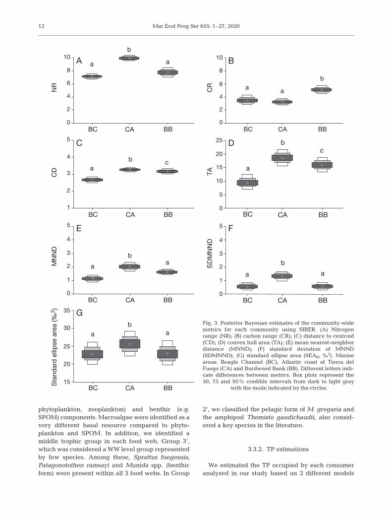
Regarding the niche widths within groups amongcommunities, the predicted SEAB showed significantdifferences (for data and pairwise comparisons seeTables S2 & S3 and Fig. 4). Specifically, with respectto inputs (Group 1), we registered a smaller isotopicniche (low SEAB) in BB, while it was larger (highSEAB) and similar in BC and CA. The zooplanktongroup (Group 2) had the smallest isotopic niche in BCand the largest niche in CA. The group formed bysmall pelagic species and crustaceans (Group 3) hadthe smallest niche in BB and the largest in CA. Bothbenthopelagic (Group 4) and demersal species(Group 5) had the lowest SEAB in BC; while G4 hadsimilar SEAB between CA and BB, and G5 had thelargest SEAB in CA. Top predators (Group 6) showedthe largest SEAB in BB and the smallest in BC.

3.3. WW species

3.3.1. Cluster analysis

The cluster analysis was useful to detect differenttrophic groups based on δ13C and δ15N values(Fig. 5). From the base to the top of each food web,the species were grouped according to their maintrophic habits and their estimated TPs. As expected,these new groups showed a different arrangement ofspecies than the SIBER groups (see Section 2.4);therefore, we identified them with a prime (‘) super-script (i.e. Group 1’, Group 2’, etc.). For example, thetop predator group (Group 6 used in SIBER) showeddiscrete groups of consumers with different TPs,such as low trophic level-foragers (e.g. whales), crus-tacean- and fish-eating taxa (e.g. seabirds and smalldolphins) and benthopelagic predators (e.g. ziphiids,pinnipeds). We detected a large overlap between thebasal groups (Groups 1’ and 2’) of pelagic (e.g.

https://www.int-res.com/articles/suppl/m655p001_supp.pdf

https://www.int-res.com/articles/suppl/m655p001_supp.pdf


24

20

14

10

2

0

A

PhytoSPOM

Cope

TG

Eupha

MGP

Sfueg

SeaB

Ctrigl

Macro

MGB

Osmitt

Emaclo

Oflav

4

6

8

12

16

18

22Aaust

Pspin

Pcorn

Pram

Ptese

–23 –22 –21 –20 –19 –18 –17 –15 –14 –13 –12 –11 –10 –8–16 –9

B

–7

–30 –29 –28 –27 –22 –20–26 –25–31–32–33 –24 –23 –21 –19 –18 –17 –16

C 20

18

16

14

12

10

8

6

4

2

0

C

Phyto

SPOM

Cope

TGEuphaMinke

MGPMS

Sfueg

PramSquid

SaustLcruc

SeaB

Ctrigl

Stene

PelegDeleg

Mmage Zcavi

Gmelas

24

20

14

10

2

0

B

Phyto

SPOM

Cope

TGEupha

MGP

SfuegPram Squid

Saust

SeaB

Ctrigl

Deleg

MacroMGB

Osmitt

Mmag

Emaclo

Ccomm

Oflav

MhubbMaust

4

6

8

12

16

18

22

–25 –24 –23 –22 –21 –20 –19 –18 –17 –16 –15 –14 –13 –12 –11

A

6

10

16

20

8

12

14

18

22

4

2

0

24

6

10

16

20

8

12

14

18

22

4

20

24

–23–22 –21 –20 –19 –18 –17 –15 –14 –13 –12 –11 –10–16 –9

–24 –23 –22 –21 –20 –19 –17 –13–18 –16 –15 –14 –12

20

18

16

14

12

10

8

6

4

2

0–30 –29 –28 –27 –20–26 –25–31 –24 –23 –22 –21 –19 –18 –17 –16

δ13C (‰) δ13C (‰)

δ13C (‰) δ13C (‰)

δ13C (‰) δ13C (‰)

δ15 N

(‰)

δ15 N

(‰)

δ15 N

(‰)

δ15 N

(‰)

δ15 N

(‰)

δ15 N

(‰)

Fig. 2. Trophic structure (left panels) and mean ± SD δ13C and δ15N values of each species/group (right panels) of (A) BeagleChannel, (B) Atlantic coast of Tierra del Fuego and (C) Burdwood Bank marine areas. Solid lines represent standard ellipse ar-eas corrected for small sample size (SEAC, fits 40% of the data). Dashed lines represent convex hull area. Black: Group 1 (in-puts: primary producers and sediment particulate organic matter), red: Group 2 (zooplankton); green: Group 3 (small pelagicfish and crustaceans); blue: Group 4 (benthopelagic species); cyan; Group 5 (mesopelagic species); magenta: Group 6 (top

predators). For species/group abbreviations, see Table 1


phytoplankton, zooplankton) and benthic (e.g.SPOM) components. Macroalgae were identified as avery different basal resource compared to phyto-plankton and SPOM. In addition, we identified amiddle trophic group in each food web, Group 3’,which was considered a WW level group representedby few species. Among these, Sprattus fuegensis,Patagonotothen ramsayi and Munida spp. (benthicform) were present within all 3 food webs. In Group

2’, we classified the pelagic form of M. gregaria andthe amphipod Themisto gaudichaudii, also consid-ered a key species in the literature.

3.3.2. TP estimations

We estimated the TP occupied by each consumeranalyzed in our study based on 2 different models

0

2

4

6

8

10N

R

BC CA BB

A

0

2

4

6

8

10

CR

BC CA BB

B

1

2

3

4

5

DC

BC CA BB

C

0

5

15

20

25

AT

10

BC CA BB

D

0

1

2

4

5

DN

NM

3

BC CA BB

E

0

1

2

4

5

DN

NM

DS

3

BC CA BB

F

15

20

25

30

35

BC CA BB

G

Stan

dard

ellip

se a

rea

(‰2 )

a a

b

a a

b

b

a

c

ab c

a ab

ab

a

a ab Fig. 3. Posterior Bayesian estimates of the community-wide

metrics for each community using SIBER. (A) Nitrogenrange (NR); (B) carbon range (CR); (C) distance to centroid(CD); (D) convex hull area (TA); (E) mean nearest-neighbordistance (MNND); (F) standard deviation of MNND(SDMNND); (G) standard ellipse area (SEAB, ‰2). Marineareas: Beagle Channel (BC), Atlantic coast of Tierra delFuego (CA) and Burdwood Bank (BB). Different letters indi-cate differences between metrics. Box plots represent the50, 75 and 95% credible intervals from dark to light gray

with the mode indicated by the circles


(Table 3, Fig. 5), but we did not find alarge difference between them. Ingeneral, lower TP estimations weremade in BC and higher estimations inCA and BB (H = 61.84, df = 2, p < 0.001and p < 0.005 for all pairwise compar-isons between the same group/spe-cies). Based on our data set, and con-sidering both models, 2 pinnipedspecies, namely South American furseal Arctocephalus australis and SouthAmerican sea lion Otaria flavescens,were the top predators in BC and O.flavescens in CA, while the long-finned pilot whale Globicephala melasoccupied the highest positions esti-mated in the oceanic BB area.

Metric Unscaled values Scaled valuesBC CA BB BC CA BB

SEA 23.62 25.59 22.85 0.03 0.04 0.03SEAC 23.72 25.72 22.98 0.03 0.04 0.03SEAB 23.50 25.50 22.90 0.03 0.04 0.04NR 7.69 9.78 7.39 0.37 0.47 0.36CR 3.04 3.17 5.16 0.09 0.10 0.16TA 8.83 19.11 15.71 0.01 0.03 0.02CD 2.67 3.27 3.13 0.12 0.15 0.14MNND 1.10 2.12 1.52 0.05 0.08 0.06SDMNND 0.65 1.09 0.72 0.03 0.04 0.02

Table 2. Isotopic niche width and Layman metrics of each community (BC:Beagle Channel; CA: Atlantic coast of Tierra del Fuego; BB: Burdwood Bank).SEA: standard ellipse area; SEAC: SEA corrected for small sample sizes; SEAB:Bayesian estimate of SEA. SEAs fit 40% of the data. NR: range in δ15N, CR:range in δ13C, TA: convex hull area, CD: mean distance to centroid, MNND:mean nearest-neighbor distance, SDMNND: standard deviation of MNND. All

metrics were calculated with unscaled and scaled values

0

5

15

Stan

dard

ellip

se a

rea

(‰2 )

Stan

dard

ellip

se a

rea

(‰2 )

Stan

dard

ellip

se a

rea

(‰2 )

Stan

dard

ellip

se a

rea

(‰2 )

Stan

dard

ellip

se a

rea

(‰2 )

Stan

dard

ellip

se a

rea

(‰2 )

BC CA BB

10

20

25

30

35

0

5

10

15

20

BC CA BB

0

5

10

15

20

BC CA BBGroup 3

BC CA BBGroup 4

0

5

10

0

5

10

15

BC CA BBGroup 5

0

5

10

15

BC CA BBGroup 6

1 puorG 2 puorG

Fig. 4. Posterior Bayesian estimates of the standard ellipse areas (SEAB, ‰2) for each functional group through SIBER. Group 1:inputs (primary producers and sediment particulate organic matter); Group 2: zooplankton; Group 3: pelagic fish and crus-taceans; Group 4: benthopelagic species; Group 5: demersal species; Group 6: top predators. Beagle Channel (BC), Atlanticcoast of Tierra del Fuego (CA) and Burdwood Bank (BB). Box plots represent the 50, 75 and 95% credible intervals from dark

to light gray. Circles correspond to the mode of SEAB for each group


The species considered in the literatureand in this study as possible WW species hadestimated TPs between 2.0 and 3.5. Overall,species in BC had lower estimated TPs com-pared to those in CA and BB (F = 15.79, df = 2,p < 0.001, for Model 1), except for T. gau-dichaudii, which showed no differences be-tween marine areas (for all pairwise compar-isons, see Table S4). The pelagic form of M.gregaria had a lower TP (ranging from 2.0 to2.2), compared to its benthic counterpart(ranging from 2.8 to 3.1). In BB, we only sam-pled 1 individual of the pelagic form, andtherefore it was not included in comparisons.However, its isotopic values resembled thoseof a pelagic organism in CA, which would ex-plain a high estimated TP (2.9, Model 1).

Within each marine area, the WW specieshad some differences between their TPs inboth models. In BB, T. gaudichaudii hadlower TPs compared to benthic Munida spin-osa, P. ramsayi and S. fuegensis, with the last3 species having similar TPs. In CA, thepelagic form of M. gregaria and T. gau-dichaudii had similar TPs, but lower withrespect to S. fuegensis and P. ramsayi. In BC,the pelagic form of M. gregaria had the low-est estimated TP and the benthic form thehighest. In addition, P. ramsayi and S. fue-gensis had similar TPs.

3.3.3. Isotopic niche widths within WWspecies groups

Within each marine area, we found differ-ences in the isotopic niche (SEAB) occupiedby the WW species considered (for data andpairwise comparisons, see Tables S5 & S6

01

23

45

SPO

M (1

)Eu

phau

siid

s (2

)M

un

ida

gre

gar

iapelag

ic(2

.)6

Th

emis

to g

aud

ich

aud

ii(2

.)3

Phyt

opla

nkto

n (1

)C

opep

ods

(2)

Cot

top

erca

trig

loid

es(3

.7)

Pat

agon

otot

hen

ram

sayi

(3.

)4Sq

uids

(3.

)4M

unid

a gr

egar

iabe

nthi

c (3

.)2

Sp

ratt

us fu

egen

sis

(3.

)5M

erlu

cciu

s au

stra

lis(

)4.

8M

erlu

cciu

s hu

bb

si(

)4.

9Se

abird

s (4

.4)

Dis

sost

ichu

s el

egin

oid

es(4

.)5

Mac

ruro

nus

mag

ella

nicu

s(4

.)1

Sal

ilota

aus

tral

is(4

.)1

Mac

roal

gae

(1)

Ota

riafla

vesc

ens

(5.

)3E

legi

nop

s m

aclo

vinu

s(4

.)4

Od

onte

sthe

s sm

itti(4

.)6

Cep

halo

rhyn

chus

com

mer

soni

i(4.

)3

Atla

ntic

coa

st o

fTie

rra d

el F

uego

(CA)

Burd

woo

d Ba

nk (B

B)

01

23

45

SPO

M (1

)

Euph

ausi

ids

(2)

Mu

nid

a g

reg

aria

pelag

ic(

)2.

9

Th

emis

to g

aud

ich

aud

ii(2

.)2

Phyt

opla

nkto

n (1

)

Cop

epod

s (2

)

Cot

top

erca

trig

loid

es(4

.)3

Pat

agon

otot

hen

ram

sayi

(3.

)5

Glo

bic

epha

la m

elas

(5.

)9

Mun

ida

spin

osa

(3.

)4

Sp

ratt

us fu

egen

sis

(3.

)5S

alilo

ta a

ustr

alis

(3.

)9

Seab

irds

(3.8

)O

cean

ic S

quid

s (3

.)5

Lage

norh

ynch

us c

ruci

ger(

3.)7

Sem

irros

ia t

ener

a(4

.)1

Pat

agon

otot

hen

eleg

ans

(4.

)3D

isso

stic

hus

eleg

inoi

des

(4.

)2

Mac

ruro

nus

mag

ella

nicu

s(

)5.

1Z

iphi

us c

aviro

stris

()

5.2

Bal

aeno

pte

rasp

- m

inke

(2.

)0

Beag

le C

hann

el (B

C)

01

23

4

Arc

toce

pha

lus

aust

ralis

(.

)4

5O

taria

flave

scen

s(

.)

4 4

Th

emis

to g

aud

ich

aud

ii(

.)

2 0

Phyt

opla

nkto

n (1

)Eu

phau

siid

s (2

)

Mu

nid

a g

reg

aria

pelag

ic(

)1.

9SP

OM

(1)

Cep

ods

(2)

op

Mac

roal

gae

(1)

Pat

agon

otot

hen

ram

sayi

(2.

)4C

otto

per

ca t

riglo

ides

(.

)2

8S

pra

ttus

fueg

ensi

s(

)2.

6M

unid

a gr

egar

iabe

nthi

c (

.)

2 8

Pat

agon

otot

hen

tess

ella

ta(

.)

2 8

Pat

agon

otot

hen

corn

ucol

a(3

.)1

Od

onte

sthe

s sm

itti(3

.)0

Pho

coen

a sp

inip

inni

s(

.)

3 3

Ele

gino

ps

mac

lovi

nus

(3.

)4Se

abird

s (3

.)5

5

Fig. 5. Cluster analysis (complete linkage methodand Euclidean distance) for 612 biological compo-nents of the 3 marine areas under study based onδ13C and δ15N values. The x-axis represents thedistance metric (Euclidean). Numbers in parenthe-ses are the estimated trophic position (TP) (Model1). The major organic primary producers and or-ganic sources (sediment particulate organic mat-ter, SPOM) are assumed to represent the firsttrophic level. The area in gray indicates the groupwith possible wasp-waist (WW) species of mid-level TPs for each marine area. Dashed boxes rep-resent different trophic groups. Species in boldhave been considered in the literature as WW

species occupying low TPs


Functional trophic Species N TP Model 1 TP model 2group/SIBER Mean SD Mode 95%CI

Lower Upper

Beagle channel (BC)Group 1: inputs Phytoplanktona 22 1.0 1.0

Macroalgae (Macrocystis pyrifera) 25 1.0 1.0SPOM 3 1.0 1.0

Group 2: zooplankton Copepodsa 19 2.0 2.0Euphausiidsa 4 2.0 2.0Munida gregaria − pelagica 11 1.9 0.4 2 2.0 2.1Themisto gaudichaudiia 4 2.0 1.0 2.2 1.5 3.0

Group 3: pelagic fish Munida gregaria − benthic 19 2.8 0.2 2.7 2.6 3.1and crustaceans Odontesthes smitti 6 3.0 0.5 2.9 2.5 3.9

Sprattus fuegensis 20 2.6 0.2 2.6 2.4 2.9Group 4: benthopelagic Patagonotothen cornucola 3 3.1 0.1 2.9 2.1 3.9

species Patagonotothen tessellata 15 2.8 0.5 2.6 2.3 3.2Patagonotothen ramsayi 4 2.4 0.2 2.3 1.9 2.6Eleginops maclovinus 20 3.4 0.2 3.4 3.2 3.7

Group 5: demersal Cottoperca trigloides 6 2.8 0.1 2.8 2.6 3.1species

Group 6: top predators Arctocephalus australisb 8 4.5 0.5 4.5 4.0 5.2Otaria flavescensb 5 4.4 0.5 4.4 4.0 5.5Phocoena spinipinnis c 1(2) 3.3 0.0 * * *Seabirds (Spheniscus magellanicus, Phala crocorax 38 3.5 0.1 3.4 3.3 3.8

atriceps, Leucophaeus scoresbii)

Atlantic coast of Tierra del Fuego (CA)Group 1: inputs Phytoplanktona 18 1.0 1.0

Macroalgae (Macrocystis pyrifera) 7 1.0 1.0SPOM 1 1.0 1.0

Group 2: zooplankton Copepodsa 14 2.0 2.0Euphausiidsa 4 2.0 2.0Munida gregaria − pelagica 7 2.6 0.4 2.2 2.0 2.6Themisto gaudichaudii 7 2.3 0.3 2.1 1.9 2.3

Group 3: pelagic fish Munida gregaria − benthica 2 3.2 0.0 * * *and crustaceans Odontesthes smitti 5 4.6 0.1 4.7 4.2 4.9

Sprattus fuegensis 11 3.5 0.4 3.4 3.0 3.6Group 4: bentho pelagic Macruronus magellanicus 5 4.1 0.1 4.1 3.7 4.4

species Patagonotothen ramsayi 19 3.4 0.2 3.4 3.1 3.6Eleginops maclovinus 9 4.4 0.3 4.5 3.8 4.9Salilota australis 13 4.1 0.5 4.1 3.6 4.4Squids (Illex argentinus, Doryteuthis gahi) 11 3.4 0.4 3.5 3.0 3.7

Group 5: demersal Cottoperca trigloides 6 3.7 0.3 3.8 2.8 4.2species Merluccius australis 14 4.8 0.2 4.7 4.5 5.1

Merluccius hubbsi 3 4.9 0.1 4.7 4.0 5.7Dissostichus eleginoides 1 4.5 * * *

Group 6: top predators Cephalorhynchus commersonii 17 4.3 0.2 4.3 4.0 4.6Otaria flavescensb 16 5.3 0.2 5.3 4.8 5.7Seabirds (Spheniscus magellanicus) 14 4.4 0.1 4.3 4.0 4.6

Burdwood Bank (BB)Group 1: inputs Phytoplanktona 10 1.0 1.0

SPOM 16 1.0 1.0Group 2: zooplankton Copepodsa 20 2.0 2.0

Euphausiidsa 22 2.0 2.0Munida gregaria − pelagica 1 2.9 * * *Themisto gaudichaudiia 21 2.2 0.3 2.2 2.0 2.9

Table 3. Trophic position (TP) estimations. Model 1: two baselines with the trophic discrimination factor (TDF) for N and C(Post 2002), Model 2: Bayesian full model with 2 baselines and TDF for N and C (Quezada-Romegialli et al. 2018). Functionaltrophic groups reported are the ones used with SIBER. Phytoplankton, macroalgae and sediment particulate organic matter(SPOM) were assigned as TP 1, and copepods and euphausiids as TP 2 in all models; ‘*’: not estimated due to low sample size(n ≤ 2). Results are shown as means ± SD for Model 1. Bayesian posterior estimates for Model 2 are shown as mode and 95%

credibility interval lower and upper limits


and Fig. 6). We did not compare the pelagic form ofM. gregaria in BB or the benthic form of the samespecies in CA due to small sample sizes. T. gau-dichaudii had the most extensive isotopic niche area(SEAB) in the 3 food webs. Also, this species over-lapped its isotopic niche only with the pelagic form ofM. gregaria, corresponding to 13 and 40% of theirrespective SEAC in BC and to 8 and 43% of theirSEAC in CA.

The isotopic niches of S. fuegensis and P. ramsayioverlapped in the 3 food webs. The overlaps corre-sponded to 98% and almost 2% of their respectiveisotopic niche area (SEAC) in BB; 13 and 25% of theirrespective SEAC in CA; and 14 and 39% of theirrespective SEAC in BC (Fig. 6). In addition, we esti-mated a wider isotopic niche area (SEAB) for P. ram-sayi than for S. fuegensis only in BB, while the oppo-site occurred in BC and CA (Tables S5 & S6).

In BC, the benthic form of M. gregaria had a highisotopic niche overlap with S. fuegensis, correspon-ding to 49 and 28% of their SEAC, and also over-lapped with P. ramsayi, but to a lesser extent, corre-sponding to 5 and 8% of their SEAC, respectively(Fig. 6).

4. DISCUSSION

The southwestern South Atlantic Ocean is a marineregion influenced by different complex oceanographicprocesses and interactions (e.g. upwelling and mixing

processes) with significant impacts on the biogeo-chemistry of the local ecosystems under study(Matano et al. 2019). By taking advantage of the iso-topic differences at a regional scale, we were able todifferentiate the 3 marine areas under study (BC, CAand BB). We utilized an appropriate isotopic baselinedetermined from a large data set of isotopic informa-tion of the biological components at the base of thefood webs (e.g. sediments, primary producers) thatcovered the full range of the isotopic variabilityrecorded in previous studies. In terms of their isotopicvalues, the BB was the most different area, character-ized by oceanic and polar conditions. We also in -cluded isotopic information of all functional trophicgroups, from the main inputs (primary producers andSPOM) to top predators (marine mammals and sea-birds). We found similar trophic metrics (e.g. topology)between the 3 food webs; however, BC and BBshowed the most pronounced WW structure (e.g.short food webs). In addition, we identified both lo-cally and regionally probable WW species. The Fue-gian sprat Sprattus fuegensis was present in all 3 ar-eas, occupying the WW level along with the longtailsouthern cod Patagonotothen ramsayi in BB and CAand with the squat lobster Munida gregaria in BC.

4.1. Baseline isotopic variation

We detected important spatial variation in carbon(δ13C) and nitrogen (δ15N) composition at the base of

Functional trophic Species N TP Model 1 TP model 2group/SIBER Mean SD Mode 95%CI

Lower Upper

Group 3: pelagic fish Munida spinosa 7 3.4 0.1 3.1 2.5 3.7and crustaceans Sprattus fuegensis 5 3.5 0.0 3.3 2.2 4.3

Group 4: bentho pelagic Macruronus magellanicus 2 5.1 0.2 3.9 2.0 6.1species Patagonotothen elegans 3 4.3 0.7 3.6 2.3 5.3

Patagonotothen ramsayi 12 3.5 0.5 3.3 3.0 4.1Salilota australis 1 3.9 * * *Semirrosia tenera 1 4.1 * * *Squid − oceanic (Gonatus antarcticus, Kondakovia 4 3.5 0.7 3 2.2 4.8

longimana)Group 5: demersal Cottoperca trigloides 10 4.3 0.5 4.1 3.8 4.7

species Dissostichus eleginoides 4 4.2 0.4 4 3.2 5.1Group 6: top predators Globicephala melas edwardii 6 5.9 0.5 5.2 4.6 6.4

Lagenorhynchus crucigerb 7 3.7 0.2 3.6 3.3 4.1Balaenoptera sp.c 1(3) 2.0 0.1 2.2 2.0 2.4Seabirds (Eudyptes chrysocome) 18 3.8 0.2 3.7 3.5 4.1Ziphius cavirostris 1 5.2 * * *

aPooled individuals in each sample; bSamples based on bone collagen; cCalf

Table 3 (continued)


the food web among the 3 marine areas under study.Chemical, physical and biological factors are knownto influence the isotopic composition of phytoplank-ton communities, which is transferred to uppertrophic levels (Graham et al. 2010). Water tempera-ture is one of the main driving forces of variability inδ13C values (Goericke & Fry 1994). In Patagonianwaters, Lara et al. (2010) found a highly significantpositive correlation between temperature and δ13Cvalues in POM towards polar waters. Since the con-centration of dissolved CO2 varies with temperature,a significant effect on isotopic fractionation by mar-ine phytoplankton is expected (Rau et al.1982, Goer-icke & Fry 1994). As with the case of carbon, theabundance and various forms of the inorganic nitro-

gen pool affect nitrogen composition, which is ruledmostly by a complex combination of different pro-cesses that occur in marine waters (e.g. the recyclingof nitrogen in the euphotic zone, N2 fixation, theinflux of nitrate-rich upwelling, nitrogen from runoffand melting glaciers) (Montoya 2007). The types ofprimary producers also introduce isotopic variation(Peterson 1999). Phytoplankton is the only primaryproducer in oceanic waters, such as the BB area.Nevertheless, high spatial and seasonal variability inthe plankton community (e.g. in terms of biomassand composition) was observed in previous studiesfrom coastal to offshore regions. Moreover, in coastalareas of BC and CA, macroalgae, which are typicallymore enriched in 13C than phytoplankton (France

Beagle Channel

Atlantic coast of Tierra del Fuego

Burdwood Bank

16

14

12

10

8

6

4–24 –22 –20 –18 –16 –14 –12 –10

δ13C (‰)

δ13C (‰)

δ13C (‰)

WW-species

WW-species

WW-species

12

10

8

6

4

0–28 –24 –22 –20 –18–26

2

50

40

20

0PramSfuegMGBMGPTG

Stan

dard

ellip

se a

rea

(‰2 )

Stan

dard

ellip

se a

rea

(‰2 )

Stan

dard

ellip

se a

rea

(‰2 )

10

0PramSfuegMGBMGPTG

5

10

0PramSfuegMSMGPTG

5

16

14

12

10

8

6

4–22 –20 –18 –16 –14

*

*

30

10

δ15 N

(‰)

δ15 N

(‰)

δ15 N

(‰)

Fig. 6. Isotopic niche of wasp-waist (WW) species for each marine area. Standard ellipse areas corrected for small sample-size(SEAC, fits 40% of the data, colored lines) and convex hull (TA, dashed lines) and posterior Bayesian estimates of the standardellipse areas (SEAB, ‰2) for each WW species per community. Box plots represent the 50, 75 and 95% credible intervals fromdark to light colors. Circles correspond to the mode of SEAB for each WW species. TG: Themisto gaudichaudii (black); MGP:Munida gregaria − pelagic (red); MGB: Munida gregaria − benthic (green); MS: Munida spinosa (green); Sfueg: Sprattus fue-

gensis (purple); Pram: Patagonotothen ramsayi (cyan). ‘*’: not estimated due to small sample size


1995, Peterson 1999), constitute an important foodsource for several benthic organisms and contributeto the pelagic realm through different pathways (e.g.grazing and suspension-feeding) (Riccialdelli et al.2017a). It is important to note that the isotope valuesregistered in the basal component of the food webs(e.g. SPOM, phytoplankton, zooplankton) can besubject to spatial and temporal variation in associa-tion with oceanographic parameters, such as sea sur-face temperatures. Although small marine organismstend to show greater temporal variability due tofaster turnover rates compared to larger organisms(Cabana & Rasmussen 1996), the isotopic variation atthe base may propagate through the entire food web.

Along the continental shelf areas of Tierra delFuego, from ~46° to ~54° S, δ13CPOM values rangesfrom −18.35 to −23.07‰ (Lara et al. 2010), whichagrees with the δ13C value of phytoplankton meas-ured in CA. We also measured δ13C values of zoo-plankton similar to values mentioned in previousstudies (e.g. −19.8‰, Ciancio et al. 2008). δ15NPOM

values range from ~5.7 to ~2.5‰, decreasing towardssouthern latitudes and reflecting biological fractiona-tion and/or isotopic differences in the nitrogen pool(Lara et al. 2010, Barrera et al. 2017). In fact, theCape Horn Current that influences the southwesternSouth Atlantic Ocean transports waters from theSouth Pacific with 15N-depleted ammonium that isavailable to phytoplankton (Lara et al. 2010). Theδ15N values that we measured in phytoplankton andzooplankton groups are in agreement with valuespreviously reported for the area (7.3‰ for δ15N, Cian-cio et al. 2008, Lara et al. 2010).

In the BC, water temperature is the main factor thatexplains most of the variation in δ13CPOM values,which are within a range of −24.5 to −20.9‰ andwith a mean value of −23.0 ± 0.9‰ (Barrera et al.2017). δ13C values measured in phytoplankton in ourstudy in BC are in agreement with the rangesreported by Barrera et al. (2017) and with a previousfood-web study that reported δ13CPOM values of −23.9± 0.7‰ and δ13Cphytoplankton values of −21.0 ± 0.5‰(Riccialdelli et al. 2017a). In addition, the availabilityof ammonium in the system (Cardona Garzón et al.2016, Barrera et al. 2017) may influence δ13Cphytoplank-

ton values due to its effect on the β-carboxylationpathway for C fixation (Dehairs et al. 1997). Also, theavailability of 15N-enriched ammonium, derived fromrunoff in the inner BC, could explain high δ15NPOM

(6.9‰), δ15Nphytoplankton (8.9 ± 0.6‰) and δ15Nmacroalgae

(10.3 ± 0.6‰) values reported previously (Barrera etal. 2017, Riccialdelli et al. 2017a) and in our study.During the austral summer, phytoplanktonic cells

like diatoms, such as Chaetoceros sp. and Thalas-siosira sp., can represent between 20 and 45% oftotal phytoplankton in coastal areas of Tierra delFuego (e.g. Almandóz et al. 2011, Barrera et al.2017). This group is the main feeding input to thezooplankton, such as copepods (e.g. Calanus aus-tralis, Oithona similis, Drepanopus forcipatus) andamphipods (e.g. Themisto gaudichaudii) (Sabatini &Álvarez Colombo 2001, Sabatini et al. 2004, Aguirreet al. 2012). Towards the open ocean, diatomsdecrease in abundance (~7%) and dinoflagellates(~93%) dominate (Barrera et al. 2017). The same pat-tern occurs during austral autumn in BC (Almandózet al. 2011).

In the oceanic BB area, complex oceanographicconditions generate an internal spatial heterogene-ity, mainly along its longitudinal axis, and conse-quently plankton communities respond with differ-ent spatial distributions (Bertola et al. 2018a, GarcíaAlonso et al. 2018). The plankton communitychanges to different pools of oceanic species of pri-mary producers (e.g. the diatom Rhizosolenia sp.,Olguín Salinas et al. 2015, Bertola et al. 2018a,b) andzooplankton like euphausiids (e.g. Euphausia lucens,E. valentini), copepods (e.g. Neocalanus tonsus) andchaetognaths (e.g. Sagitta spp.) (Sabatini & ÁlvarezColombo 2001, Sabatini et al. 2004, Aguirre et al.2012). Interestingly, satellite color imagery showedgenerally lower chlorophyll blooms over BB withrespect to coastal areas like CA and BC (Matano etal. 2019). However, in BB, phytoplankton blooms candevelop in deeper layers and not on the surface(Bertola et al. 2018a). Our isotopic data in that areaare similar to published information for zooplanktonof the Antarctic Circumpolar Current (e.g. euphausi-ids range from −26.0 to −22.0‰ and from 3.5 to 5.3‰for δ13C and δ15N, respectively; Schmidt et al. 2003,Stowasser et al. 2012). Between the shelf and oceanicsub-Antarctic waters, from ~55° to ~58° S, meanδ13CPOM values were −26.93 ± 0.61‰ (Lara et al.2010), near what we measured for marine phyto-plankton in BB (−26.1 ± 4.3‰). δ15N POM values alsodecrease within a range of 1 to 4‰ and drop to −1.6to 1‰ at the Drake Passage (Lara et al. 2010). Theseare waters of low temperatures (~5.1°C) and salini-ties (~34), where the Malvinas Current, the main cur-rent that influences the BB marine area, originates(Matano et al. 2019). In agreement with previousstudies in oceanic and southern waters (e.g. Schmidtet al. 2003, Lara et al. 2010, Stowasser et al. 2012), wealso measured low δ15Nphytoplankton values (3.8 ±0.04‰) in BB. The main reason for the low δ15N valuein these waters seems to be the phytoplankton


uptake of isotopically light ammonium that comesfrom oceanic zooplankton excretions and the intensemineralization of the organic matter in surfacewaters (Lara et al. 2010). Thus, the BB area is influ-enced by typical oceanic and polar water masses,characterized by very low δ13C and δ15N values thatcreate a unique marine area compared to the otherinvestigated areas.

4.2. Trophic structure

Based on the scaling procedure, the unbiased sta-ble isotope space showed reduced differencesbetween communities (Cucherousset & Villéger2015), but did not blur the quantification of the esti-mated trophic community metrics and allowed us toidentify large-scale patterns in food-web organiza-tion across the 3 marine areas. Interestingly, thetopologies of the food webs and the associated iso-topic community metrics showed similar results withand without scaling the data. This was due to the factthat the full range in δ13C (min−max = 25‰) and δ15N(min−max = 21‰) values among the 3 marine areaswas similar, with a difference between both axis ofonly 4‰.

The food webs were quite similar among the 3 mar-ine areas studied in terms of structure, species com-position and clustering, although we found some dif-ferences. Across a latitudinal gradient, the topologyof Patagonian food webs exhibits a reduction in ver-tical structure and trophic diversity towards thesouth (Saporiti et al. 2015), meaning that food webstend to be shorter and more redundant towards sub-polar and polar waters as an outcome of a more pro-nounced WW structure (Ducklow et al. 2007, Saporitiet al. 2014). We evaluated the topology of food websmainly in a longitudinal axis, from inshore (BC, CA)to offshore waters (BB). However, among the 3 foodwebs studied, CA is closer to central and northernPatagonia and was the area that showed metrics sim-ilar to the southern area studied by Saporiti et al.(2015). From CA towards BB and BC, a more pro-nounced WW structure was evident in the isotopicmetrics. Marine areas can differ in species composi-tion and functional groups, and therefore spatial seg-regation of taxa can influence food-web topology(Montoya et al. 2015). Overall, we found shorterfood-chain lengths at BB and BC, compared to CA.Few pelagic/benthopelagic species, such as S. fue-gensis, M. gregaria, P. ramsayi and T. gaudichaudii,are known to dominate the mid to low TPs in thissouthern region (Padovani et al. 2012, Arkhipkin &

Laptikhovsky 2013, Diez et al. 2016, 2018). The highabundance of few prey species at this level of thefood web (e.g. Saporiti et al. 2015) imposes a certainfeeding dependence on southern predators, shortensfood-web length and increases the trophic overlapand redundancy of the overall food web (Cury et al.2000). Several mesopredators in the CA area (e.g.hakes Merluccius hubbsi and M. australis, amongothers) represent important links of mobile andlarge-bodied species with different trophic habitsincreasing the food-chain length, reducing interspe-cific niche overlap and trophic redundancy in thismarine area. Therefore, higher consumers can diver-sify their diet, thereby increasing omnivory and gen-eralism (e.g. Nye et al. 2020).

In addition, higher habitat heterogeneity, as wellas warmer and more productive marine areas, cansustain a higher number of species with differentfeeding strategies that require high resource avail-ability (Kortsch et al. 2019). Such environmentalconditions have been positively associated withfood-web complexity metrics (Saporiti et al. 2015,Kortsch et al. 2019). We found low trophic diversitywith lower CD values compared to those reportedby Saporiti et al. (2015), considering that we havetaken into account top predator data (i.e. marinemammals and seabirds), which may increase Lay-man metrics. Among the 3 marine areas studied,BC and BB had the most restricted trophic diversityand a high trophic redundancy and evenness, aswould be expected towards Antarctic waters. Theseresults are in agreement with the smaller isotopicniche area occupied by these communities. Limitedprimary productivity and lower temperatures, suchas those occurring in polar waters, reduce food-web complexity, which is sustained by smaller-sized fish and crustaceans acting as important linksbetween lower and higher trophic levels (Kortschet al. 2019). This scenario is in agreement withenvironmental conditions in BC and BB (Lara et al.2010, Almandóz et al. 2011, Barrera et al. 2017,Matano et al. 2019). In combination, all of thesemetrics and SEA analyses imply a slightly morestructurally complex food web in CA, compared tothe BB and BC marine areas.

Food-web structure, as well as the type of controlthat can be operating in a given marine area, is adynamic process linked to the presence and distribu-tion of species in a community (Young et al. 2015).Our findings may also contribute to the understand-ing of the structure of ancient food webs at coastalareas. A number of retrospective studies have exam-ined food web changes over time based on the iso-


topic analysis of skeletal remains of marine faunafrom shell middens in the southwestern AtlanticOcean (e.g. Saporiti et al. 2014, Zangrando et al.2016, Vales et al. 2017, Bas et al. 2019, 2020, Nye etal. 2020). Specifically, a reduction in the basal struc-ture characterizes modern and coastal food webs,when compared to ancient ones (e.g. Saporiti et al.2014, Bas et al. 2019). Higher temperatures in thepast could have caused more freshwater run-off anda major supply of C3 plant debris being input intocoastal marine waters (Bas et al. 2019). Since C3plant debris is 13C-depleted compared to marinephytoplankton and macroalgae (Riccialdelli et al.2017a), its greater contribution may have increasedthe range of δ13C baseline values measured in thepast.

Furthermore, in our study, BB showed significantlylower δ13C values and a broader basal structure com-pared to coastal areas. In BB, multiple primaryresource types do not cause the isotopic variationmeasured at the base of its food web, since phyto-plankton seems to be the only primary producer.Instead, other main driving forces have been identi-fied, including water temperature (see Section 4.1).Consequently, a greater influence of oceanic watersin coastal areas could also have helped to spread therange in basal structure of ancient food webs.

In addition, a higher vertical structure was esti-mated for modern food webs compared to ancientones (Saporiti et al. 2014, Bas et al. 2019). This differ-ence is related to a change in the foraging strategy ofpinnipeds between pre- and post-hunting settings.Reductions in their populations produced a release ofinter- and intraspecific competition that may haveled to the consumption of more benthic and highertrophic level prey with respect to the ones consumedin the past in the same habitat (Vales et al. 2017, Baset al. 2019). An increase in trophic diversity and adecrease in trophic redundancy was reportedbetween ancient and modern food webs in coastalareas and was explained by a trophic segregationbetween species of marine mammals and seabirdstowards modern times (Saporiti et al. 2014, Bas et al.2019). Warmer (e.g. Argentine hake M. hubbsi, Baset al. 2020) and oceanic shoaling pelagic species (e.g.snoek Thyrsites atun, Zangrando et al. 2016) mayhave played an important role as WW species in thepast. If this group of species was a common prey fortop predators, this would explain the overlap in theirisotopic niches found in the past (e.g. Bas et al. 2019).However, at present, these species are not commonin shallow waters and could have been replaced byother WW species, such as S. fuegensis. Further-

more, ancient food webs were reconstructed with askewed vision of the isotopic baselines of the openwaters adjacent to Tierra del Fuego. In light of ourdata set, oceanic fish had lower δ15N values com-pared to coastal ones. Thus, if oceanic species hadbeen common prey also inhabiting coastal areas inthe past (e.g. T. atun), a higher consumption of these15N-depleted prey, but at high TPs (Zangrando et al.2016), would offer another possible explanation forthe change registered in nitrogen stable isotope val-ues in top predators from ancient to modern foodwebs. Climatic variation may affect the distributionof these oceanic prey through time (Bas et al. 2019),thereby altering trophic interactions along coastalareas of Tierra del Fuego. This scenario is in synergywith modern human impacts that may have pushedtop predators to forage in greater areas, increasingthe range of dietary sources and niche size over time(Nye et al. 2020). Future studies should furtherexplore these hypotheses. The present research pro-vides crucial background information regardingmodern isotopic niche space and topologies of foodwebs to understand the effects of different naturaland/or anthropogenic impacts, during past andfuture settings.

4.3. WW species

TP estimates represent a powerful metric to com-pare the position of each species/group and thewhole food-chain length among regions and timeperiods (Young et al. 2015). The estimation of TP isparticularly important in WW ecosystems, since theavailability of a few species has profound conse-quences on the entire food web. The TDFs used inthis study are an important aspect in the estimationof TP and food change length. TDFs range widelyamong animals, in relation to the tissue analyzed, thespecies, the nutritional condition of the animal, thequality of diet and body size, among many other fac-tors (Post 2002). We acknowledge that the use offixed values of TDF oversimplified trophic structure(e.g. food-web length) and species interactions(Hussey et al. 2014). However, we analyzed manyspecies that have a poorly characterized diet andtherefore we had the same bias in the 3 food websanalyzed. Furthermore, we estimated TPs with 2 dif-ferent models with no substantial differencesbetween them.

Within the 3 marine areas under study, a mid-trophic level group (WW level) formed by smallpelagic and benthopelagic species that feed on the


planktivorous fraction and constitute a link to upperconsumers, was identified through the cluster analy-sis. In addition to this middle group, 2 lower trophiclevel species, the hyperiid amphipod Themisto gau-dichaudii and the pelagic form of Munida gregaria,have been suggested by previous studies to also beimportant links to upper consumers (e.g. Padovani etal. 2012, Diez et al. 2016, 2018). As has beenobserved across the major WW ecosystems of theworld, the WW level can be dominated by the coexis-tence of 2 or more (but still relatively few) WW spe-cies that alternate, due to fluctuations in their abun-dances (Bakun & Broad 2003). The fluctuation ofthese populations has been visible on multi-annualtime scales mainly attributed to a set of factors,including climate variability, density-dependent pro-cesses and fishing pressure (Bakun 2006). Thus,when the dominant species declines, the subordinateopportunistically replaces the first. The species weconsidered to be WW in the studied areas exhibiteddifferences in their isotopic niche, such as nichewidth and TP estimated. Thus, the availability ofthese WW species may have important implicationsin the structure of the overall trophic webs, by affect-ing their putative predators and their own prey, ashas been detected between ancient and modern foodwebs in the region.

In our study case, the Fuegian sprat constitutes theonly pelagic species with abundances high enoughto be considered the most important species in thetrophodynamics of CA and BC (Sánchez et al. 1995,Madirolas et al. 2000, Sabatini et al. 2004, Diez et al.2018). In addition, it is an important prey item formany top marine predators in the region (e.g. RayaRey et al. 2007, Riccialdelli et al. 2013, Scioscia et al.2014, Haro et al. 2016, Harris et al. 2016). TheMPAN-BB has also been identified as a major spawn-ing and nursery ground for S. fuegensis (GarcíaAlonso et al. 2018).

We analyzed adult individuals collected in BB (dur-ing cruise VA1418 in November), and a school of S.fuegensis was sighted during winter in the area (L.Riccialdelli pers. obs., BOPDAGO-2018). The lowδ13C and δ15N values of muscle from these individu-als indicate a feeding period in the oceanic food webof BB, but not in any other area near it (e.g. CA orBC), or even in the nearest marine environment ofthe Falkland/Malvinas Islands (see Quillfeldt et al.2015). The importance of S. fuegensis in each marinearea seems to be a clear consequence of its specialposition in the food webs as has been seen for otherpelagic organisms in other marine regions (e.g. krillin Antarctic waters, Ducklow et al. 2007, Jordán

2009). Furthermore, based on our estimations, S. fue-gensis exhibited different estimated TPs (with thelowest in BC), but occupied mid to low TPs in all 3study areas, meaning that it has a similar trophic rolein a regional context. Myctophids are known to be adominant mesopelagic group at a tertiary level inoceanic waters that play a key role in pelagic foodwebs (Saunders et al. 2014). In the BB area, larvalstages of myctophids have been collected onboardthe same research vessels used in the present work(D. Bruno unpubl data), but neither juvenile noradult stages were collected with the used fishinggear. Thus, for now, S. fuegensis constitutes the onlypelagic planktivorous species in the BB area, andbased on the isotope values, this population couldrepresent a different stock from the coastal sprat, atleast from an ecological point of view. However, fur-ther studies should be conducted to investigate thispossibility.

The longtail southern cod is one of the mostabundant benthopelagic nototheniids in southernPatagonia, including BB, and also constitutes animportant prey for meso and top consumers(Arkhipkin & Laptikhovsky 2013). This species canfeed over a wide range of planktonic (e.g. cope-pods, T. gaudichaudii, euphausiids, jellyfish andsalps) and benthic organisms (e.g. Munida spp.,isopods, amphipods) and can easily switch dietfrom plankton to benthos (Laptikhovsky & Arkhip-kin 2003, Arkhipkin & Laptikhovsky 2013). Thisplasticity in the diet explains the broader isotopicniche area that characterized our isotopic data setin relation to this species. In the BB and CA areas,P. ramsayi was the most abundant fish collectedduring the research cruises. Its isotopic niche alsodoes not overlap entirely with that of S. fuegensisin any of these marine areas, and thus this speciesand sprat are the 2 most important WW species inboth areas.

Several species of Patagonotothen are also presentin BC; however, they are mostly benthic and coastalspecies (Ceballos et al. 2019). In addition, during theresearch cruises, we collected only a few individualsof P. ramsayi with the bottom trawling operations inthis area. The squat lobster M. gregaria is one of themost abundant crustaceans and is prey for many spe-cies in BC and southern Patagonia (e.g. Scioscia et al.2014, Diez et al. 2016). This species also links thebenthic and the pelagic realm, contributing to thevertical carbon flow. In particular, M. gregaria has 2morphotypes, ‘subrugosa’ with full benthic habits asadults and ‘gregaria’ that has both pelagic and ben-thic forms during the adult stage (Lovrich & Thiel


2011). The pelagic form of M. gregaria occurs at highdensities in BC (Diez et al. 2016, 2018) in an analo-gous manner to Antarctic krill Euphausia superba inAntarctic waters (Ducklow et al. 2007).

Polar water zooplankton, like copepods and krill,tend to accumulate lipids for overwintering andreproduction (Hagen & Auel 2001). M. gregariastores lipids mainly in the hepatopancreas and usesthis energy supply for reproduction and molting(Romero et al. 2006). Burkholder et al. (1967) foundthat M. gregaria from Tierra del Fuego had a higherfat content and caloric value than Antarctic krill. M.gregaria and S. fuegensis had similar energy density(7.15 vs. 7.5 kJ g−1, respectively; Romero et al. 2006,Ciancio et al. 2007, Scioscia et al. 2014), much higherthan all the fishes reported to date in BC (4.21−6.26 kJ g−1, Fernández et al. 2009). These estimationswere made on benthic Munida. Until now, there hasbeen no proximal analysis or energy density estima-tion made on the pelagic form. However, to remain inthe water column, the pelagic form reduces its den-sity by increasing its water content and reducing ashand calcium content (Lovrich & Thiel 2011). Also, itoptimizes its energetic budget with a higher capacityfor aerobic metabolism than the benthic form (C.Avalos & G. Lovrich unpubl. data, cited by Lovrich &Thiel 2011), which may directly influence its fat stor-age. In addition, in Baja California, Smith et al.(1975) found no differences in chemical compositionbetween the pelagic and benthic form of Pleuron-codes planipes, a key species in that system.

Furthermore, the availability of pelagic swarms ofM. gregaria has increased in terms of occurrence andabundance over the last 10 yr in BC and southernPatagonia (Diez et al. 2016, 2018). Hydroacoustic sur-veys revealed that pelagic aggregations of M. gre-garia and S. fuegensis occur in BC throughout theyear. However, a negative and more intense interac-tion between them seems to occur during summer,when they showed greater spatial overlap (Diez et al.2018). In this sense, the pelagic form of M. gregariaconstitutes an easy and highly valuable energysource, and thus may constitute an important preyitem in the diet of upper consumers, which requirehigh prey concentrations to gain energy.

In BC, previous studies have found no isotopic dif-ferences between the benthic forms of both morpho-types (‘subrugosa’ and ‘gregaria’), having similar TPestimations (Pérez Barros et al. 2010, Riccialdelli etal. 2017a) to each other and to those from northernPatagonian waters (e.g. San Jorge Gulf, Funes et al.2018). We estimated lower TPs for the pelagic stageof ‘gregaria’ than for the benthic form. The same pat-

tern was reported by Funes et al. (2018) in the SanJorge Gulf, which could be the result of the differentcontribution of the pelagic and benthic energy path-ways in the food webs. The TP occupied by bothforms/stages (pelagic and benthic) gives them animportant role in potentially shortening the food-weblength.

In this way, M. gregaria and S. fuegensis can beconsidered WW species in light of their mid to lowTPs and because of the key role they play in terms ofenergy transfer in the trophodynamics of the BCarea. In the BB area, we analyzed only 1 sample ofpelagic M. gregaria, which is not common in thearea. In contrast, the species commonly found in BBare fully benthic forms, M. spinosa and M. gregaria‘subrugosa’ (not analyzed), which probably play thesame trophic role as their benthic counterparts in CAand BC.

The functional group of mesopredators, such as thePatagonian grenadier Macruronus magellanicus,Argentine and southern hakes, Patagonian toothfishDissostichus eleginoides, southern blue whitingMicromesistius australis and thornfish Cottopercatrigloides, are also important for the food-web struc-ture (being both predators and prey). As juveniles,these species can at least temporally dominate theWW level, but as adults, they became semi-demersalor demersal predators (Bakun 2006). These meso-predators may constitute an important alternate foodsupply available to top predators in CA (Bas et al.2020, Nye et al. 2020), where we found a more com-plex system than in the BC and BB areas (e.g. highervalues of community-wide metrics).

4.4. Top predators

Generally, seabirds and marine mammals are con-sidered top predators. However, based on our esti-mations, they occupied from the third to the fifth TPs.The highest positions in the oceanic BB were occu-pied by offshore cetaceans, such as long-finned pilotwhales. Offshore predators are known to have wideforaging grounds, and thus high estimated SEAB,preferring the Patagonian slope break around is -lands and upwelling areas, such as the ones wefound around the BB area (Riccialdelli et al. 2010,2017b). Meanwhile in coastal ecosystems, SouthAmerican sea lions and South American fur sealswere the most important and highest predators of theanalyzed food webs, as also reported in previousstudies (Drago et al. 2009, Vales et al. 2017). Animportant point to consider is the fact that both spe-


cies are known to forage on a wide range of habitatsfrom inshore to offshore areas, thereby increasingtheir isotopic niche (Nye et al. 2020).

Meanwhile, coastal dolphins (e.g. Commerson’sdolphin Cephalorhynchus commersonii) and por-poises (e.g. Burmeister’s porpoise), seabirds (e.g. cor-morants, penguins) and oceanic whales (e.g. Bal-aenoptera sp.) mainly feed on mid to low trophiclevel species (Riccialdelli et al. 2010, 2013, Raya Reyet al. 2012, Scioscia et al. 2014, Haro et al. 2016, Har-ris et al. 2016). Thus they exhibit lower TPs, as wefound in this study and in accordance with previousinformation. Minke whale samples were consideredas a proxy for oceanic whales that are known to for-age on small pelagic crustaceans (euphausiids) insub-Antarctic and Antarctic waters (Van Waerebeeket al. 2010), and consequently occupy low TPs. How-ever, other species of whales like fin whales Bal-aenoptera physalus that have been seen in the BBarea (N. Dellabianca unpubl. data), or humpbackwhales Megaptera novaeangliae, a common ceta -cean for the Fuegian archipelago, are known to for-age on pelagic crustaceans (euphausiids and pelagicM. gregaria) and small pelagic fish (S. fuegensis)(Haro et al. 2016). Thus, as we expected, these spe-cies occupy mid-level TPs as a reflection of theirknown diet.

Since many top predators can be considered gen-eralists, their ability to exert top-down control maydepend on the variety of alternate prey species avail-able to them (Madigan et al. 2012), but also woulddepend on the distances they move and how muchtime they spend foraging in each marine area interms of inshore versus offshore waters. Nonetheless,the WW species considered for each area may consti-tute an important part of predator diets; they alsodepend on a wide variety of prey species, such asbenthic organisms that were not considered in theirfull context in this study, but that contribute to a highlevel of omnivory.

4.5. Concluding remarks

In light of our results, the BC and BB areas seem tohave a more pronounced WW structure than CA.Identifying the most influential species in these foodwebs is particularly important to maintain ecosystemintegrity and the supply of ecosystem services(Jordán 2009). WW species can be considered asmajor interactors, having many links to other mem-bers of the food web. A long-term plan for managingbiodiversity loss should focus on the protection of

these species, but also on key areas for them. Thefact that BB has been identified as a spawning andnursery ground for S. fuegensis and P. ramsayi, con-sidered as 2 WW species in a regional context, givesthis oceanic sector additional relevance for conser -vation. It is necessary to continue to use differentapproaches to identify unusually important or influ-ential species and specific areas of importance forthem (e.g. spawning areas). In addition, continuingwith the examination of regional variation and long-term changes (e.g. responses to top-down and bot-tom-up forces) is crucial to systematically compileinformation on the integrity, structure and function-ing of these subpolar ecosystems in a way that wouldhelp to assess the potential short- and long-term con-sequences of natural and anthropogenic impacts.

Acknowledgements. We are indebted to the MPA Namun -curá − Burdwood Bank administration and CONICET foreconomic support and logistics. We are grateful to captainsand crews of the RVs ‘Puerto Deseado’, ‘SB-15 Tango’ and‘Victor Angelescu’, and also to M. Perez, L. Pagnosin and R.Saenz Samaniego, pilots of the CADIC boat ‘Don Pedro’, fortheir assistance during the surveys. Special thanks to G. A.Lovrich, Scientific Coordinator of the MPA Namuncurá- Burdwood Bank, the whole Burdwood Bank scientific groupand the scientific chief of each survey, i.e. G. A. Lovrich(BOPD-Mar2014), N. A. Dellabianca (Tango-Feb2015), D.Roccatagliata (BOPD-Abr2016), G. Colombo and M. J. Diez(VA1418). We also thank M. L. Presta (plankton), M. J. Diezand G. A. Lovrich (Crustacea), S. G. Ceballos and P. A. Vil-latarco (fish) and N. A. Dellabianca (marine mammals), whoprovided their expertise on the identification or confirma-tion of different taxa analyzed. The IMMA Project and RNPGoodall Foundation provided information (date and site ofdeath) for marine mammal specimens. E. Ducós (INGEIS),G. Quiroga, A. Dauverne and A. Gil (LIECA-Mendoza)aided with the isotopic analyses. We especially thank C. B.Anderson who helped revise the English text, as well asRodrigo Bastos and 2 anonymous referees, who helped withconstructive revisions. This study was funded by the MPANamuncurá (Law 26875), the Agencia Nacional de Promo-ción Científica y Tecnológica (PICT 2012-1832, PICT 2013-2228, PICT 2016-0195) and CONICET (PIP-440, PUE 2016CADIC). This work is contribution no. 34 of the MPANamuncurá (Law 26875).

LITERATURE CITED

Abrantes KG, Barnett A, Bouillon S (2014) Stable isotope-based community metrics as a tool to identify patterns infood web structure in east African estuaries. Funct Ecol28: 270−282

Acha EM, Mianzan HW, Guerrero RA, Favero M, Bava J(2004) Marine fronts at the continental shelves of australSouth America: physical and ecological processes. J MarSyst 44: 83−105

Aguirre GE, Capitanio FL, Lovrich GA, Esnal GB (2012)Seasonal variability of metazooplankton in coastal sub-

https://doi.org/10.1111/1365-2435.12155

https://doi.org/10.1080/17451000.2011.627922

https://doi.org/10.1016/j.jmarsys.2003.09.005


Antarctic waters (Beagle Channel). Mar Biol Res 8: 341−353

Almandóz GO, Hernando MP, Ferreyra GA, Schloss IR, Fer-rario ME (2011) Seasonal phytoplankton dynamics inextreme southern South America (Beagle Channel,Argentina). J Sea Res 66: 47−57

Alvito PM, Rosa R, Phillips RA, Cherel Y and others (2015)Cephalopods in the diet of nonbreeding black-browedand grey-headed albatrosses from South Georgia. PolarBiol 38: 631−641

Arkhipkin A, Laptikhovsky V (2013) From gelatinous tomuscle food chain: rock cod Patagonotothen ramsayirecycles coelenterate and tunicate resources on thePatagonian Shelf. J Fish Biol 83: 1210−1220

Bakun A (2006) Wasp-waist populations and marine ecosys-tem dynamics: navigating the “predator pit” topogra-phies. Prog Oceanogr 68: 271−288

Bakun A, Broad K (2003) Environmental ‘loopholes’ and fishpopulation dynamics: comparative pattern recognitionwith focus on El Niño effects in the Pacific. FishOceanogr 12: 458−473

Balestrini C, Manzella G, Lovrich G (1998) Simulación decorrientes en el Canal Beagle y Bahía Ushuaia, medianteun modelo bidimensional. Informe técnico no. 98. Depar-tamento de Oceanografía, Buenos Aires

Barrera F, Lara RJ, Krock B, Garzón-Cardona JE, Fabro E,Koch BP (2017) Factors influencing the characteristicsand distribution or surface organic matter in thePacific−Atlantic connection. J Mar Syst 175: 36−45

Bas M, Briz i Godino I, Álvarez M, Vales DG, Crespo EA,Cardona L (2019) Back to the future? Late Holocene mar-ine food web structure in a warm climatic phase as a pre-dictor of trophodynamics in a warmer South-WesternAtlantic Ocean. Glob Change Biol 25: 404−419

Bas M, Salemme M, Green EJ, Santiago F and others (2020)Predicting habitat use by the argentine hake Merlucciushubbsi in a warmer world: inferences from the MiddleHolocene. Oecologia 193: 461−474

Belkin IM, Cornillon PC, Sherman K (2009) Fronts in largemarine ecosystems. Prog Oceanogr 81: 223−236

Bertola G, Olguín Salinas H, Iachetti CM, Lovrich GA,Alder VA (2018a) Estructura del plancton unicelulareucariota del AMP Namuncurá—Banco Burdwood enprimavera: conexiones con las adyacencias. In: Meno -ret A, Guller M (eds) Libro de resúmenes X JNCM,Buenos Aires, p 74

Bertola G, Olguín Salinas H, Alder VA (2018b) Distribucionespecial de Rhizosolenia crassa, ¿especie clave del BancoBurdwood? In: Menoret A, Guller M (eds) Libro deresúmenes X JNCM, Buenos Aires, p 73

Burkholder PR, Mandelli EF, Centeno P (1967) Some chem-ical properties of Munida gregaria and Euphausiasuperba. J Agric Food Chem 15: 718−720

Cabana G, Rasmussen JB (1996) Comparison of aquatic foodchains using nitrogen isotopes. Proc Natl Acad Sci USA93: 10844−10847

Cardona L, Martínez-Iñigo L, Mateo R, González-Solís J(2015) The role of sardine as prey for pelagic pre -dators in the western Mediterranean Sea assessedusing stable isotopes and fatty acids. Mar Ecol ProgSer 531: 1−14

Cardona Garzón JE, Martínez AM, Barrera F, Pfaff F andothers (2016) The Pacific−Atlantic connection: biogeo-chemical signals in the southern end of the Argentineshelf. J Mar Syst 163: 95−101

Ceballos SG, Roesti M, Matschiner M, Fernández DA, Dam-erau M, Hanel R, Salzburger W (2019) Phylogenomics ofan extra-Antarctic notothenioid radiation reveals a pre-viously unrecognized lineage and diffuse species bound-aries. BMC Evol Biol 19: 13

Ciancio JE, Pascual MA, Beauchamp DA (2007) Energydensity of Patagonian aquatic organisms and empiricalpredictions based on water content. Trans Am Fish Soc136: 1415−1422

Ciancio JE, Pascual MA, Botto F, Frere E, Iribarne O (2008)Trophic relationships of exotic anadromous salmonids inthe southern Patagonia shelf as referred from stable iso-topes. Limnol Oceanogr 53: 788−798

Constable AJ, Melbourne-Thomas J, Corney SP, ArrigoKR and others (2014) Climate change and SouthernOcean ecosystems I: how changes in physical habitatsdirectly affect marine biota. Glob Change Biol 20: 3004−3025

Coplen TB, Krouse HR, Böhlke JK (1992) Reporting of nitro-gen-isotope abundances. Pure Appl Chem 64: 907−908

Cucherousset J, Villéger S (2015) Quantifying the multiplefacets of isotopic diversity: new metrics for stable isotopeecology. Ecol Indic 56: 152−160

Cury P, Bakun A, Crawford RJM, Jarre A, Quiñones RA,Shannon LJ, Verheye HM (2000) Small pelagics inupwelling systems: patterns of interaction and structuralchanges in “wasp-waist” ecosystems. ICES J Mar Sci 57: 603−618

Cury P, Shannon L, Shin YJ (2003) The functioning of mar-ine ecosystems: a fisheries perspective. In: Sinclair M,Valdimarsson G (eds) Responsible fisheries in the marineecosystem. CABI Publishing, Wallingford, p 103−123

Dehairs F, Kopczynska E, Nielsen P, Lancelot C, BakkerDCE, Koeve W, Goeyens L (1997) δ13C of SouthernOcean suspended organic matter during spring andearly summer: regional and temporal variability. DeepSea Res II 44: 129−142

Demopoulos AWJ, McClain-Counts J, Ross SW, Brooke S,Mienis F (2017) Food-web dynamics and isotopic nichesin deep-sea communities residing in a submarine canyonand on the adjacent open slopes. Mar Ecol Prog Ser 578: 19−33

Diez MJ, Cabreira AG, Madirola A, Lovrich GA (2016)Hydroacoustical evidence of the expansion of pelagicswarms of Munida gregaria (Decapoda, Munididae) inthe Beagle Channel and the Argentine Patagonian Shelf,and its relationship with habitat features. J Sea Res 114: 1−12

Diez MJ, Cabreira AG, Madirolas A, Martín de NascimentoJ, Scioscia G, Schiavini A, Lovrich GA (2018) Winter iscool: spatio-temporal patterns of the squat lobsterMunida gregaria and the Fuegian sprat Sprattus fuegen-sis in a sub-Antarctic estuarine environment. Polar Biol41: 2591−2605

Drago M, Crespo EA, Aguilar A, Cardona L, Garcia N, DansSL, Goodall N (2009) Historic diet change of the SouthAmerican sea lion in Patagonia as revealed by isotopicanalysis. Mar Ecol Prog Ser 384: 273−286

Ducklow HW, Baker K, Martinson DG, Quetin LB and others(2007) Marine pelagic ecosystems: the west AntarcticPeninsula. Philos Trans R Soc B 362: 67−94

Falabella V (ed) (2017) Área Marina Protegida Namuncurá—Banco Burdwood. Contribuciones para la línea de base yel plan de manejo. Jefatura de Gabinete de Ministros,Buenos Aires

https://doi.org/10.1016/j.seares.2011.03.005

https://doi.org/10.1007/s00300-014-1626-3

https://doi.org/10.1111/jfb.12217

https://doi.org/10.1016/j.pocean.2006.02.004

https://doi.org/10.1046/j.1365-2419.2003.00258.x


https://doi.org/10.1111/gcb.14523

https://doi.org/10.1007/s00442-020-04667-z


https://doi.org/10.1021/jf60152a037

https://doi.org/10.1073/pnas.93.20.10844

https://doi.org/10.3354/meps11353


https://doi.org/10.1098/rstb.2006.1955


https://doi.org/10.1007/s00300-018-2394-2



https://doi.org/10.1016/S0967-0645(96)00073-2

https://doi.org/10.1006/jmsc.2000.0712

https://doi.org/10.1016/j.ecolind.2015.03.032

https://doi.org/10.1351/pac199264060907

https://doi.org/10.1111/gcb.12623

https://doi.org/10.4319/lo.2008.53.2.0788

https://doi.org/10.1577/T06-173.1

https://doi.org/10.1186/s12862-019-1345-z


Fernández DA, Lattuca ME, Boy CC, Pérez AF and others(2009) Energy density of sub-Antarctic fishes from theBeagle Channel. Fish Physiol Biochem 35: 181−188

France RL (1995) Carbon-13 enrichment in benthic com-pared to planktonic algae: foodweb implications. MarEcol Prog Ser 124: 307−312

Francey RK, Allison CE, Etheridge DM, Trudinger CM andothers (1999) A 1000-year record of δ13C in atmosphericCO2. Tellus B Chem Phys Meterol 51: 170−193

Funes M, Irigoyen AJ, Trobbiani GA, Galván DE (2018) Sta-ble isotopes reveal different dependencies on benthicand pelagic pathways between Munida gregaria eco-types. Food Webs 17: e00101

García Alonso VA, Brown D, Martin J, Pájaro M, Capi-tanio FL (2018) Seasonal patterns of Patagonian spratSprattus fuegensis early life stages in an open seaSub-Antarctic Marine Protected Area. Polar Biol 41: 2167−2179

Goericke R, Fry B (1994) Variations of marine plankton δ13Cwith latitude, temperature, and dissolved CO2 in theworld ocean. Global Biogeochem Cycles 8: 85−90

Gonfiantini R (1978) Standards for stable isotope measure-ments in natural compounds. Nature 271: 534−536

Graham BS, Koch PL, Newsome SD, McMahon KW, Auri-oles D (2010) Using isoscapes to trace the movementsand foraging behavior of top predators in oceanic ecosys-tems. In: West J (ed) Isoscapes: understanding move-ment, pattern, and process on earth through isotopemapping. Springer, Berlin, p 299−318

Hagen W, Auel H (2001) Seasonal adaptations and therole of lipids in oceanic zooplankton. Zoology 104: 313−326

Haro D, Riccialdelli L, Acevedo J, Aguayo-Lobo A, MontielA (2016) Trophic ecology of humpback whales(Megaptera novaeangliae) in the Magellan Strait as indi-cated by carbon and nitrogen stable isotopes. AquatMamm 42: 233−244

Harris D, Horwáth WR, van Kessel C (2001) Acid fumigationof soils to remove carbonates prior to total organic carbonor carbon-13 isotopic analysis. Soil Sci Soc Am J 65: 1853−1856

Harris S, Sáenz Samaniego RA, Raya Rey A (2016) Insightsinto diet and foraging behaviour of imperial shags (Pha-lacrocorax atriceps) breeding at Staten Island andBecassess Islands, Tierra del Fuego, Argentina. Wilson JOrnithol 128: 811−820

Hedges REM, Stevens RE, Koch PL (2005) Isotopes in bonesand teeth. In: Leng MJ (ed) Isotopes in palaeoenviron-mental research. Springer, Dordrecht, p 117−145

Hoegh-Guldberg O, Bruno JF (2010) The impact of climatechange on the world’s marine ecosystems. Science 328: 1523−1528

Hunt GL Jr, McKinnell S (2006) Interplay between top-down, bottom-up, and wasp-waist control in marine eco-systems. Prog Oceanogr 68: 115−124

Hussey NE, MacNeil MA, McMeans BC, Olin JA and others(2014) Rescaling the trophic structure of marine foodwebs. Ecol Lett 17: 239−250

Isla F, Bujalesky G, Coronato A (1999) Procesos estuarinosen el Canal Beagle, Tierra del Fuego. Rev Asoc GeolArgent 54: 307−318

Jackson AL, Inger R, Parnell AC, Bearhop S (2011) Compar-ing isotopic niche widths among and within communi-ties: SIBER—Stable Isotope Bayesian Ellipses in R. JAnim Ecol 80: 595−602

Jordán F (2009) Keystone species and food webs. PhilosTrans R Soc B 364: 1733−1741

Kortsch S, Primicerio R, Aschan M, Lind S, Dolgov AV,Planque B (2019) Food-web structure varies along envi-ronmental gradients in a high-latitude marine ecosys-tem. Ecography 42: 295−308

Laptikhovsky VV, Arkhipkin AI (2003) An impact of sea-sonal squid migrations and fishing on the feeding spectraof subantarctic notothenioids Patagonotothen ramsayiand Cottoperca gobio around Falkland Islands. J ApplIchthyol 19: 35−39

Lara RJ, Alder V, Franzosi CA, Kattner G (2010) Character-istics of suspended particulate organic matter in thesouthwestern Atlantic: influence of temperature, nutri-ent and phytoplankton features on the stable isotope sig-nature. J Mar Syst 79: 199−209

Layman CA, Arrington DA, Montaña CG, Post DM (2007)Can stable isotope ratios provide for community-widemeasures of trophic structure? Ecology 88: 42−48

Lovrich GA, Thiel M (2011) Ecology, physiology, feedingand trophic role of squat lobsters. In: Poor GCB, AhyongST, Taylor J (eds) The biology of squat lobsters. CSIROPublishing, Collingwood, p 183–222

Lynam CP, Llope M, Möllmann C, Helaouët C, Bayliss-Brown GA, Stenseth NC (2017) Interaction between top-down and bottom-up control in marine food webs. ProcNatl Acad Sci USA 114: 1952−1957

Madigan DJ, Carlisle AB, Dewar H, Snodgrass OE, LitvinSY, Micheli F, Block BA (2012) Stable isotope analysischallenges wasp-waist food web assumptions in anupwelling pelagic ecosystem. Sci Rep 2: 654

Madirolas A, Sánchez R, Hansen J, Alvarez Colombo G,Reta R (2000) Distribución, abundancia, biología y hábi-tat de la sardina fueguina (Sprattus fuegensis). Tech Rep.INIDEP, Mar del Plata

Matano RP, Palma ED, Combes V (2019) The BurdwoodBank circulation. J Geophys Res Oceans 124: 6904−6926

Montoya D, Yallop ML, Memmott J (2015) Functional groupdiversity increases with modularity in complex foodwebs. Nat Commun 6: 7379

Montoya JP (2007) Natural abundance of 15N in marineplanktonic ecosystems. In: Michener R, Lajthka K (eds)Stable isotopes in ecology and environmental science.Blackwell Publishing, Malden, MA, p 176−201

Newsome SD, Chivers SJ, Berman Kowalewski M (2018)The influence of lipid-extraction and long-term DMSOpreservation on carbon (δ13C) and nitrogen (δ15N) iso-tope values in cetacean skin. Mar Mamm Sci 34: 277−293

Nye JW, Zangrando AFJ, Martinoli MP, Fogel ML (2020)Temporal and population trends in human exploited pin-nipeds from Tierra del Fuego. Palaeogeogr Palaeoclima-tol Palaeoecol 554: 109804

Olguín Salinas HF, Brandini F, Boltovskoy D (2015) Latitudi-nal patterns and interannual variations of spring phyto-plankton in relation to hydrographic conditions of thesouthwestern Atlantic Ocean (34°−62°S). Helgol Mar Res69: 177−192

Padovani L, Viñas MD, Sánchez F, Mianzan H (2012)Amphipod-supported food web: Themisto gaudichaudii,a key food resource for fishes in the southern PatagonianShelf. J Sea Res 67: 85−90

Parnell AC, Inger R, Bearhop S, Jackson AL (2010) Sourcepartitioning using stable isotopes: coping with too muchvariation. PLOS ONE 5: e9672

https://doi.org/10.1007/s10695-008-9234-1


https://doi.org/10.3402/tellusb.v51i2.16269

https://doi.org/10.1016/j.fooweb.2018.e00101

https://doi.org/10.1007/s00300-018-2352-z

https://doi.org/10.1029/93GB03272

https://doi.org/10.1038/271534a0

https://doi.org/10.1078/0944-2006-00037

https://doi.org/10.1578/AM.42.2.2016.233

https://doi.org/10.2136/sssaj2001.1853

https://doi.org/10.1676/15-141.1

https://doi.org/10.1126/science.1189930


https://doi.org/10.1111/ele.12226

https://doi.org/10.1371/journal.pone.0009672


https://doi.org/10.1007/s10152-015-0427-6

https://doi.org/10.1016/j.palaeo.2020.109804

https://doi.org/10.1111/mms.12454

https://doi.org/10.1038/ncomms8379

https://doi.org/10.1029/2019JC015001

https://doi.org/10.1038/srep00654

https://doi.org/10.1073/pnas.1621037114

https://doi.org/10.1890/0012-9658(2007)88%5b42%3ACSIRPF%5d2.0.CO%3B2


https://doi.org/10.1046/j.1439-0426.2003.00340.x

https://doi.org/10.1111/ecog.03443

https://doi.org/10.1098/rstb.2008.0335

https://doi.org/10.1111/j.1365-2656.2011.01806.x


Payo-Payo A, Ruiz B, Cardona L, Borrell A (2013) Effect oftissue decomposition on stable isotope signatures ofstriped dolphins Stenella coeruleoalba and loggerheadsea turtles Caretta caretta. Aquat Biol 18: 141−147

Pérez-Barros P, Romero MC, Calcagno JA, Lovrich GA(2010) Similar feeding habits of two morphs of Munidagregaria (Decapoda) evidence the lack of trophic poly-morphism. Rev Biol Mar Oceanogr 45: 461−470

Peterson BJ (1999) Stable isotopes as tracers of organic mat-ter input and transfer in benthic food webs: a review.Acta Oecol 20: 479−487

Piola AR, Rivas AL (1997) Corrientes en la PlataformaContinental. In: Boschi EE (ed) El Mar Argentino ysus recursos pesqueros. Tomo I. INIDEP, Mar delPlata, p 119−132

Post DM (2002) Using stable isotopes to estimate trophicposition: models, methods, and assumptions. Ecology 83: 703−718

Post DM, Layman CA, Albrey Arrington D, Takimoto G,Quattrochi J, Montaña CG (2007) Getting to the fat of thematter: models, methods and assumptions for dealingwith lipids in stable isotope analyses. Oecologia 152: 179−189

Quezada-Romegialli C, Jackson AL, Hayden B, KahilainenKK, Lopes C, Harrod C (2018) TROPHICPOSITION, an Rpackage for the Bayesian estimation of trophic positionfrom consumer stable isotope ratios. Methods Ecol Evol9: 1592−1599

Quillfeldt P, Ekschmitt K, Brickle P, McGill RAR, Wolters V,Dehnhard N, Masello JF (2015) Variability of highertrophic level stable isotope data in space and time—acase study in a marine ecosystem. Rapid Commun MassSpectrom 29: 667−674

R Development Core Team (2019) R: a language and envi-ronment for statistical computing. R Foundation for Sta-tistical Computing, Vienna

Rau GH, Sweeney RE, Kaplan IR (1982) Plankton 13C: 12Cratio changes with latitude: differences betweennorthern and southern oceans. Deep-Sea Res A 29: 1035−1039

Rau GH, Mearns AJ, Young DR, Olson RJ, Schafer HA,Kaplan IR (1983) Animal 13C/12C correlates with trophiclevel in pelagic food webs. Ecology 64: 1314−1318

Raya Rey A, Trathan P, Schiavini A (2007) Inter-annual vari-ation in provisioning behaviour of southern rockhopperpenguins Eudyptes chrysocome chrysocome at StatenIsland, Argentina. Ibis 149: 826−835

Raya Rey A, Polito M, Archuby D, Coria N (2012) Stable iso-topes identify age- and sex-specific dietary partitioningand foraging habitat segregation in southern giantpetrels breeding in Antarctica and southern Patagonia.Mar Biol 159: 1317−1326

Reisinger RR, de Bruyn PJN, Bester MN (2011) Predatoryimpact of killer whales on pinniped and penguin popula-tions at the Subantarctic Prince Edward Islands: fact andfiction. J Zool (Lond) 285: 1−10

Riccialdelli L, Newsome SD, Fogel ML, Goodall RNP (2010)Isotopic assessment of prey and habitat preferences of acetacean community in the southwestern South AtlanticOcean. Mar Ecol Prog Ser 418: 235−248

Riccialdelli L, Newsome SD, Dellabianca NA, Bastida R,Fogel ML, Goodall RNP (2013) Ontogenetic diet shiftin Commerson’s dolphin (Cephalorhynchus commer-sonii commersonii) off Tierra del Fuego. Polar Biol 36: 617−627

Riccialdelli L, Newsome SD, Fogel ML, Fernández DA(2017a) Trophic interactions and food web structureof a subantarctic marine food web in the BeagleChannel: Bahía Lapatia, Argentina. Polar Biol 40: 807−821

Riccialdelli L, Paso Viola MN, Panarello HO, Goodall RNP(2017b) Evaluating the isotopic niche of beaked whalesfrom the southwestern South Atlantic and SouthernOceans. Mar Ecol Prog Ser 581: 183−198

Romero MC, Lovrich GA, Tapella F (2006) Seasonal changesin dry mass and energetic content of Munida subrugosa(Crustacea: Decapoda) in the Beagle Channel,Argentina. J Shellfish Res 25: 101−106

Sabatini ME, Álvarez Colombo GL (2001) Seasonal patternof zooplankton biomass in the Argentinian shelf offSouthern Patagonia (45°−55°S). Sci Mar 65: 21−31

Sabatini M, Reta R, Matano R (2004) Circulation and zoo-plankton biomass distribution over the southern Patag-onian shelf during late summer. Cont Shelf Res 24: 1359−1373

Sánchez RP, Remeslo A, Madirolas A, de Ciechomski JD(1995) Distribution and abundance of post-larvae andjuveniles of the Patagonian sprat, Sprattus fuegensis,and related hydrographic conditions. Fish Res 23: 47−81

Saporiti F, Bearhop S, Silva L, Vales DG and others (2014)Longer and less overlapping food webs in anthropogeni-cally disturbed marine ecosystems: confirmations fromthe past. PLOS ONE 9: e103132

Saporiti F, Bearhop S, Vales DG, Silva L and others (2015)Latitudinal changes in the structure of marine food websin the Southwestern Atlantic Ocean. Mar Ecol Prog Ser538: 23−34

Saunders RA, Collins MA, Foster E, Shreeve R, Stowasser G,Ward P, Tarling GA (2014) The trophodynamics of South-ern Ocean Electrona (Myctophidae) in the Scotia Sea.Polar Biol 37: 789−807

Schmidt K, Atkinson A, Stübing D, McClelland JW, Mon-toya JP, Voss M (2003) Trophic relationships amongSouthern Ocean copepods and krill: some uses and limi-tations of a stable isotope approach. Limnol Oceanogr48: 277−289

Scioscia G, Raya Rey A, Saenz Samaniego RA, Florentín O,Schiavini A (2014) Intra- and interannual variation in thediet of the Magellanic penguin (Spheniscus magellani-cus) at Martillo Island, Beagle Channel. Polar Biol 37: 1421−1433

Smith KL Jr, Harbison GR, Rowe GT, Clifford CH (1975)Respiration and chemical composition of Pleuroncodesplanipes (Decapoda: Galatheidae): energetic signifi-cance in an upwelling system. J Fish Res Board Can 32: 1607−1612

Stowasser G, Atkinson A, McGill RAR, Phillips RA, CollinsMA, Pond DW (2012) Food web dynamics in the ScotiaSea in summer: a stable isotope study. Deep Sea Res II59: 60208−60221

Thompson RM, Brose U, Dunne JA, Hall RO Jr and others(2012) Food webs: reconciling the structure and functionof biodiversity. Trends Ecol Evol 27: 689−697

Vales DG, Cardona L, Zangrando AF, Borella F and others(2017) Holocene changes in the trophic ecology of anapex marine predator in the South Atlantic Ocean.Oecologia 183: 555−570

Van Waerebeek K, Leaper R, Baker AN, Papastavrou V andothers (2010) Odontocetes of the Southern Ocean Sanc-tuary. J Cetacean Res Manag 11: 315−346

https://doi.org/10.3354/ab00497

https://doi.org/10.4067/S0718-19572010000300011

https://doi.org/10.1016/S1146-609X(99)00120-4

https://doi.org/10.1890/0012-9658(2002)083%5b0703%3AUSITET%5d2.0.CO%3B2

https://doi.org/10.1007/s00442-006-0630-x

https://doi.org/10.1111/2041-210X.13009

https://doi.org/10.1002/rcm.7145

https://doi.org/10.1016/0198-0149(82)90026-7

https://doi.org/10.2307/1937843

https://doi.org/10.1111/j.1474-919X.2007.00718.x

https://doi.org/10.1007/s00227-012-1912-y

https://doi.org/10.1007/s00227-012-1912-y

https://doi.org/10.1111/j.1469-7998.2011.00815.x


https://doi.org/10.1007/s00300-013-1289-5

https://doi.org/10.1007/s00442-016-3781-4

https://doi.org/10.1016/j.tree.2012.08.005

https://doi.org/10.1016/j.dsr2.2011.08.004

https://doi.org/10.1139/f75-186

https://doi.org/10.1007/s00300-014-1532-8

https://doi.org/10.4319/lo.2003.48.1.0277

https://doi.org/10.1007/s00300-014-1480-3


https://doi.org/10.1371/journal.pone.0103132

https://doi.org/10.1016/0165-7836(94)00339-X

https://doi.org/10.1016/j.csr.2004.03.014

https://doi.org/10.3989/scimar.2001.65n121

https://doi.org/10.2983/0730-8000(2006)25%5b101%3ASCIDMA%5d2.0.CO%3B2


https://doi.org/10.1007/s00300-016-2007-x


Wada E, Mizutani H, Minagawa M (1991) The use of stableisotopes for food web analysis. Crit Rev Food Sci Nutr 30: 361−371

Widdicombe S, Somerfield PJ (2012) Marine biodiversity: itspast, development, present status, and future threats. In: Solan M, Aspden RJ, Paterson DM (eds) Marine biodi-versity and ecosystem functioning. Oxford UniversityPress, Oxford, p 1–15

Young JW, Hunt BPV, Cook TR, Llopiz JK and others (2015)The trophodynamics of marine top predators: currentknowledge, recent advances and challenges. Deep SeaRes II 113: 170−187

Zangrando AF, Riccialdelli L, Kochi S, Nye JW, Tessone A(2016) Stable isotope evidence supports pelagic fishingby hunter-gatherers in southern South America duringthe Late Holocene. J Archaeol Sci Rep 8: 486−491

Editorial responsibility: Alejandro Gallego,Aberdeen, UK

Reviewed by: R. Bastos and 2 anonymous referees

Submitted: March 1, 2020 Accepted: October 5, 2020Proofs received from author(s): November 19, 2020

https://doi.org/10.1080/10408399109527547

https://doi.org/10.1016/j.jasrep.2016.05.015

https://doi.org/10.1016/j.dsr2.2014.05.015

Trophic structure of southern marine ecosystems

Documents