Trend of Seasonal and Annual Rainfall in Semi-arid Districts ...

Page 1/22

Trend of Seasonal and Annual Rainfall in Semi-arid Districts of Karnataka,India: Application of Innovative Trend Analysis ApproachKK Chowdari Surajit Deb Barma  ( [email protected] )

National Institute of Technology Karnataka https://orcid.org/0000-0003-0849-3033Nagaraj Bhat R Girisha K.C. Gouda Amai Mahesha 

Research Article

Keywords:

Posted Date: March 16th, 2022

DOI: https://doi.org/10.21203/rs.3.rs-1447773/v1

License: This work is licensed under a Creative Commons Attribution 4.0 International License.   Read Full License

Page 2/22

AbstractTrend analysis of rainfall is often carried out in water resources management to understand its distribution over a given region. The cumulative seasonaland annual rainfall derived from monthly datasets spanning 102 years (1901–2002) for 11 districts of the semi-arid Karnataka, India, was used for thetrend analysis. The two-step homogeneous test approach was carried out on all the time series. Then, lag-1 autocorrelation was conducted only onhomogeneous time series. Only 78.18% of the total time series data was detected as homogeneous, and 95.35% of time series data were found to haveinsigni�cant autocorrelation. Then, the Innovative Trend Analysis (ITA) method was applied to 43 homogeneous rainfall time series, MK and SR tests to41 time series, and mMK test to two time series. The MK and SR tests detected 14.63% of the time series as a signi�cant trend, whereas the ITA methodcould detect 93.02% of the total time series data. The MK and SR tests captured signi�cant trends for the winter season in two districts, but the two testsdetected a signi�cant trend only in one district for the summer season. None could be captured for monsoon season. A signi�cant trend was captured forthe post-monsoon season in two districts; however, the tests could detect a signi�cant trend in one district for annual rainfall. The mMK test revealed apositive trend for the post-monsoon season in a district. The ITA method could capture a signi�cant trend for all the seasons in most districts.

1 IntroductionThe demand for fresh water is ever increasing because of the myriad of needs that are encountered daily in different sectors. Its availability andoccurrences result from the quantum of precipitation received during a given period. Even groundwater, which forms a signi�cant source of fresh water inmany parts of the world, is recharged by rainfall. Therefore, precipitation is the major component of the hydrologic cycle. One peculiar characteristic ofprecipitation is that its occurrence is uneven over space and time (Sansom et al. 2017). The precipitation occurrence can lead to �ood (drought) when itis excess (scanty). For example, the recent occurrences of devastating �oods of 2018 in Kerala (Mishra and Nagaraju 2019) and 2021 in Germany(Fekete and Sandholz 2021) remind how costly precipitation can be when it occurs in excess. On the other extreme, some parts of the United States ofAmerica (USA) experienced signi�cant drought during 2020 (Yaddanapudi and Mishra 2022), and 2021 also shows the continuation of the drought inother parts of the USA. It is also known that scanty rainfall leads to meteorological drought (Sajeev et al. 2021; Muthuvel and Mahesha 2021). Thisdrought is often the precursor to agricultural drought (Behrang Manesh et al. 2019) and hydrological drought (Hao et al. 2016). This erratic behaviour ofrainfall calls for a proper understanding of rainfall distribution in space and time. Moreover, it is imperative to understand the precipitation trend due toanthropogenic activities and climate alteration in the hydrologic cycle (Zhang et al. 2007; Wu et al. 2013; Yi et al. 2016).

One of the ways to understand the distribution of rainfall patterns over an area of interest is the trend analysis that helps us ascertain how much rainfallamount increases or decreases on a particular time scale. The most widely used nonparametric methods to capture monotonic trends are the Mann-Kendall (MK) and Spearman’s rho (SR) methods (Kendall 1938; Mann 1945; Daniel 1990). Some of the recent studies on the use of MK and SR tests forrainfall trend analysis have been reported in the literature (Kalra and Ahmad 2011; Abghari et al. 2013; Gocic and Trajkovic 2013; Formetta et al. 2016;Güner Bacanli 2017; Hajani et al. 2017; Pandey and Khare 2018; Nikzad Tehrani et al. 2019; Raja and Aydin 2019; Gado et al. 2019). However, the MK andSR approaches are limited to the assumptions of the absence of serial correlation (autocorrelation) of a given time series of a variable, normaldistribution of the time series, and the sample size of the data. In order to circumvent the requirement of the limiting assumptions, Şen (2012) proposedthe innovative trend analysis (ITA) method for carrying out trend investigation of hydrometeorological variables. The ITA method also does not requirethe prewhitening of time series data prior to applying it. Since then, several studies on the ITA method have been conducted for trend analysis ofhydrometeorological variables in different regions. For example, Güçlü (2018a) extended the ITA method to half time series method (HTSM) that couldaid the ITA method to detect trend analysis better.

Similarly, the same author proposed double-ITA (D-ITA) and triple-ITA (T-ITA) approaches to use in tandem with ITA to improve trend detection withstability identi�cation (Güçlü 2018b). In yet another study, innovative triangular trend analysis (ITTA) that aids in detecting partial trends within a giventime series was applied using the triangular array after splitting a given time series to a pair of equal length sub-series to make a comparison of trends(Güçlü et al. 2020). The extended version of ITA – the Innovative Polygonal Trend Analysis (IPTA) can not only detect trends captured by the traditionalmethods but also trend transitions of a time scale (weekly, monthly, etc.) of two equal sub-series derived from the original data (Şen et al. 2019). Inextending the IPTA, Ceribasi et al. (2021) proposed the Innovative Trend Pivot Analysis Method (ITPAM) to determine the �ve risk classes using theinherent relationship in data.

Despite the extended versions of the ITA method in literature, the original ITA method (Şen 2012, 2017a) is still widely used for trend analysis ofhydrometeorological variables, as evident from recent literature. For instance, Harka et al. (2021) carried out a comparative study of MK, and ITAapproaches to detect rainfall trends in Ethiopia's Upper Wabe Shebelle River Basin (UWSRB). The ITA test detected both monotonic and non-monotonictrends that could not have been possible with the MK test. In a similar study of the Bumbu watershed, Papua New Guinea, Doaemo et al. (2022) did acomparative study of rainfall trend analysis using linear regression, Mann-Kendall rank statistics, Sen’s Slope, and ITA. In addition, spectral analysis wascarried out to remove cyclic components from the rainfall time series. Their �ndings, however, indicate that all the four methods consistently indicateddecreasing trend of annual rainfall. Several other studies on ITA application are reported in the literature (Danandeh Mehr et al. 2021; Şişman and Kizilöz2021; Mallick et al. 2021; Phuong et al. 2022; Ay 2022). The extended version of ITA - IPTA is the most widely used method to detect trends and trendtransitions of different hydrometeorological variables (Şan et al. 2021; Ceribasi and Ceyhunlu 2021; Ahmed et al. 2021; Akçay et al. 2021; Hırca et al.2022).

The occurrences of �ood and drought events in India (Mishra and Nagaraju 2019; Mishra et al. 2021; Jha et al. 2021) cause economic losses and life.Therefore, the need for �ood policy (Jameel et al. 2020) and understanding the effect of historical and future drought on crops (Udmale et al. 2020) is

Page 3/22

necessary for effective water management. There is an urgent need to address these issues because most of the population depends on agriculture asan occupation. In this regard, rainfall trend analysis will help the country with pragmatic decisions and actionable plans in dealing with both �oods anddrought. The MK test has been widely used to study monthly, seasonal, and annual rainfall trends in India both at the national (Kumar et al. 2010;Nengzouzam et al. 2020; Kaur et al. 2021) and regional levels (Goyal 2014; Gajbhiye et al. 2016; Chatterjee et al. 2016; Meshram et al. 2017; Pandey andKhare 2018; Mehta and Yadav 2021; Gupta et al. 2021).

Recent studies on precipitation trend analysis in India witnessed the ITA method being increasingly applied. Often the ITA method has been comparedwith MK, SR, and linear regression methods (Sanikhani et al. 2018; Machiwal et al. 2019; Meena et al. 2019; Praveen et al. 2020; Singh et al. 2021a; Sainiand Sahu 2021; Aher and Yadav 2021). A few studies are worth mentioning using the ITA and classical trend analysis methods at the national level. Thestudy by Praveen et al. (2020) presented the rainfall trend analysis of all the meteorological sub-divisions of India from 1901 to 2015 at the seasonal andannual scales. It was noticed that the change detection point conducted using the Pettitt test was mostly found to be after 1960 for the meteorologicaldivisions. The application of the MK test revealed the trend to be positive during 1901–1950; however, the trend reduced after 1951. The ITA methoddetected mostly negative trends even when the MK test detected no trend. Singh et al. (2021) presented a similar study of the same region using griddedrainfall data (1901 to 2019), both seasonal and annual. The ITA method was compared with MK, modi�ed Mann-Kendall (mMK), and the linearregression analysis (LRA) tests.

Interestingly, the ITA method could detect trends beyond traditional approaches. An increasing trend was observed for the monsoon and annual rainfall inthe northwest and peninsular India; however, the northeast central portion of the nation experienced a negative trend. Most of the zones, however,experienced decreasing winter rainfall. Extracting the rainfall events from anomalous rainfall time series (1871–2016), Saini and Sahu (2021) carried outa unique (not raw rainfall time series) study for the same meteorological zones of India using the MK, ITA, and LRA methods. Though the study is uniquein terms of data input and detailed, re�ned trend analysis, the ITA test captured other trends similar to the above mentioned studies.

The ITA method can be used to capture the trend in hydrometeorological time series data overcoming the assumptions of traditional trend analysisapproaches. However, the requirement of time series homogeneity cannot be neglected (Şen 2012). However, there are limited studies on using the ITAapproach on homogeneous rainfall time series in the Indian context. If homogeneity tests are not carried out, there are chances of accepting false trends,which might not have occurred.

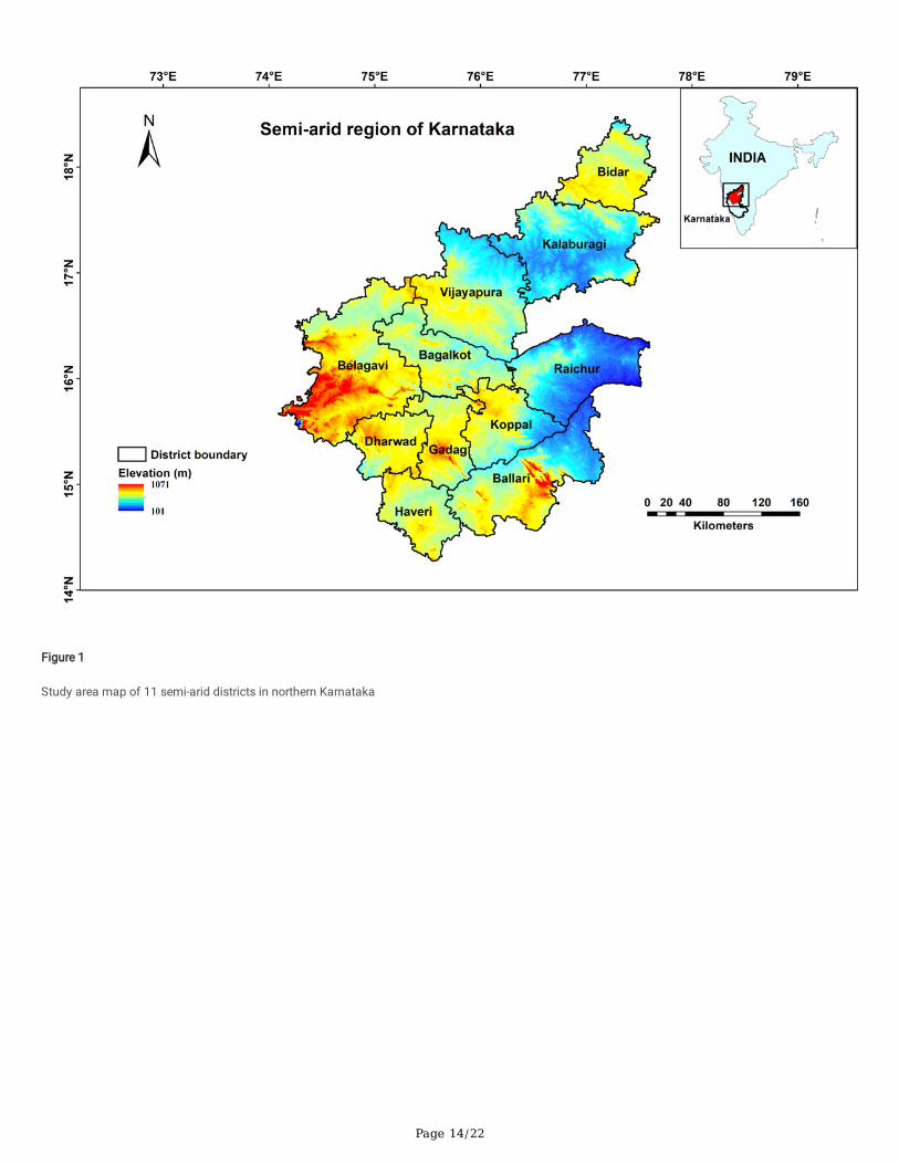
Karnataka stands only next to Rajasthan state in India to be the most drought-prone area (Jayasree and Venkatesh 2015), receiving a little over 700 mmof mean annual rainfall. The northern region of the state, Rajasthan and northern-central Maharashtra constitute 72% of India's total pearl milletproduction (Singh et al. 2017). The region is also home to some of the largest crop-producing districts in Karnataka. The districts in this region lie on theWestern Ghats' leeward side, making them drought-prone. Furthermore, nearly 90% of the inhabitants in the semi-arid region of Karnataka - over andabove 11 districts are dependent on agriculture as an occupation (Jayasree and Venkatesh 2015).

From the literature, it is evident that no such study on the ITA method for precipitation trend analysis has been reported for this region. Hence, the presentinvestigation is focused on: (a) to carry out homogeneity tests of seasonal and annual rainfall time series of each district within the region, (b) todetermine the serial correlation of each time series, and (c) to compare the trend of seasonal and annual rainfall using the MK, mMK, SR, and ITAapproaches.

2 Study AreaThe semi-arid region, also known as North Interior Karnataka, lies between 14.26 °N to 18.49 °N latitude and 74.07 °E to 77.71 °E longitude, with anelevation of about 100 to 1100 m above msl (Fig. 1). It has 11 districts, namely Bagalkot, Belagavi (Belgaum), Ballari (Bellary), Bidar, Vijayapura (Bijapur),Dharwad, Gadag, Kalaburagi (Gulbarga), Haveri, Koppal, and Raichur. The region makes up 84,560 km2, which is about 44% of the area of the state. Thepopulation is over 23 million (about 40%) (https://www.census2011.co.in/district.php). There are four seasons in the state of Karnataka in a year:January and February- winter, March to May- summer, June to September- monsoon, and October to December- post-monsoon. The temperature rangesbetween 5–25°C during the winter and 20–40°C during the summer. Though the temperature drops during the monsoon, the rise in humidity level couldcause the weather to be unpleasant. The post-monsoon and winter seasons are generally pleasant. The district of Raichur experienced the lowest meanof total annual rainfall at 564 mm, while the district of Dharwad experienced the highest mean of total annual rainfall at 2233 mm (1901–2002). Theregion receives about 80% of the total annual rainfall during the southwest monsoon (June - September). The most commonly grown crops in the regionare paddy, jowar, sugarcane, cotton, and �nger millet (ragi).

Figure 1 Study area map of 11 semi-arid districts in northern Karnataka

3 Data And Methods

3.1 Data usedThe monthly rainfall data of 11 districts (Fig. 1) of semi-arid Karnataka were retrieved from the India water portal(http://www.indiawaterportal.org/metdata) spanning 102 years (1901–2002). The monthly rainfall data at the district level have been applied for trendanalysis for different regions across India (Chatterjee et al. 2016; Meshram et al. 2017; Pandey and Khare 2018; Sharma and Goyal 2020; Mahato et al.2021). Each monthly time series dataset was further summed up to obtain seasonal and annual rainfall time series.

Page 4/22

3.2 Methods

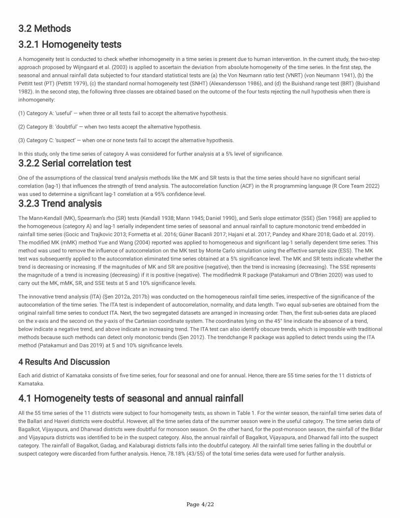
3.2.1 Homogeneity testsA homogeneity test is conducted to check whether inhomogeneity in a time series is present due to human intervention. In the current study, the two-stepapproach proposed by Wijngaard et al. (2003) is applied to ascertain the deviation from absolute homogeneity of the time series. In the �rst step, theseasonal and annual rainfall data subjected to four standard statistical tests are (a) the Von Neumann ratio test (VNRT) (von Neumann 1941), (b) thePettitt test (PT) (Pettitt 1979), (c) the standard normal homogeneity test (SNHT) (Alexandersson 1986), and (d) the Buishand range test (BRT) (Buishand1982). In the second step, the following three classes are obtained based on the outcome of the four tests rejecting the null hypothesis when there isinhomogeneity:

(1) Category A: ‘useful’ — when three or all tests fail to accept the alternative hypothesis.

(2) Category B: ‘doubtful’ — when two tests accept the alternative hypothesis.

(3) Category C: ‘suspect’ — when one or none tests fail to accept the alternative hypothesis.

In this study, only the time series of category A was considered for further analysis at a 5% level of signi�cance.

3.2.2 Serial correlation testOne of the assumptions of the classical trend analysis methods like the MK and SR tests is that the time series should have no signi�cant serialcorrelation (lag-1) that in�uences the strength of trend analysis. The autocorrelation function (ACF) in the R programming language (R Core Team 2022)was used to determine a signi�cant lag-1 correlation at a 95% con�dence level.

3.2.3 Trend analysisThe Mann-Kendall (MK), Spearman’s rho (SR) tests (Kendall 1938; Mann 1945; Daniel 1990), and Sen’s slope estimator (SSE) (Sen 1968) are applied tothe homogeneous (category A) and lag-1 serially independent time series of seasonal and annual rainfall to capture monotonic trend embedded inrainfall time series (Gocic and Trajkovic 2013; Formetta et al. 2016; Güner Bacanli 2017; Hajani et al. 2017; Pandey and Khare 2018; Gado et al. 2019).The modi�ed MK (mMK) method Yue and Wang (2004) reported was applied to homogeneous and signi�cant lag-1 serially dependent time series. Thismethod was used to remove the in�uence of autocorrelation on the MK test by Monte Carlo simulation using the effective sample size (ESS). The MKtest was subsequently applied to the autocorrelation eliminated time series obtained at a 5% signi�cance level. The MK and SR tests indicate whether thetrend is decreasing or increasing. If the magnitudes of MK and SR are positive (negative), then the trend is increasing (decreasing). The SSE representsthe magnitude of a trend is increasing (decreasing) if it is positive (negative). The modi�edmk R package (Patakamuri and O’Brien 2020) was used tocarry out the MK, mMK, SR, and SSE tests at 5 and 10% signi�cance levels.

The innovative trend analysis (ITA) (Şen 2012a, 2017b) was conducted on the homogeneous rainfall time series, irrespective of the signi�cance of theautocorrelation of the time series. The ITA test is independent of autocorrelation, normality, and data length. Two equal sub-series are obtained from theoriginal rainfall time series to conduct ITA. Next, the two segregated datasets are arranged in increasing order. Then, the �rst sub-series data are placedon the x-axis and the second on the y-axis of the Cartesian coordinate system. The coordinates lying on the 45° line indicate the absence of a trend,below indicate a negative trend, and above indicate an increasing trend. The ITA test can also identify obscure trends, which is impossible with traditionalmethods because such methods can detect only monotonic trends (Şen 2012). The trendchange R package was applied to detect trends using the ITAmethod (Patakamuri and Das 2019) at 5 and 10% signi�cance levels.

4 Results And DiscussionEach arid district of Karnataka consists of �ve time series, four for seasonal and one for annual. Hence, there are 55 time series for the 11 districts ofKarnataka.

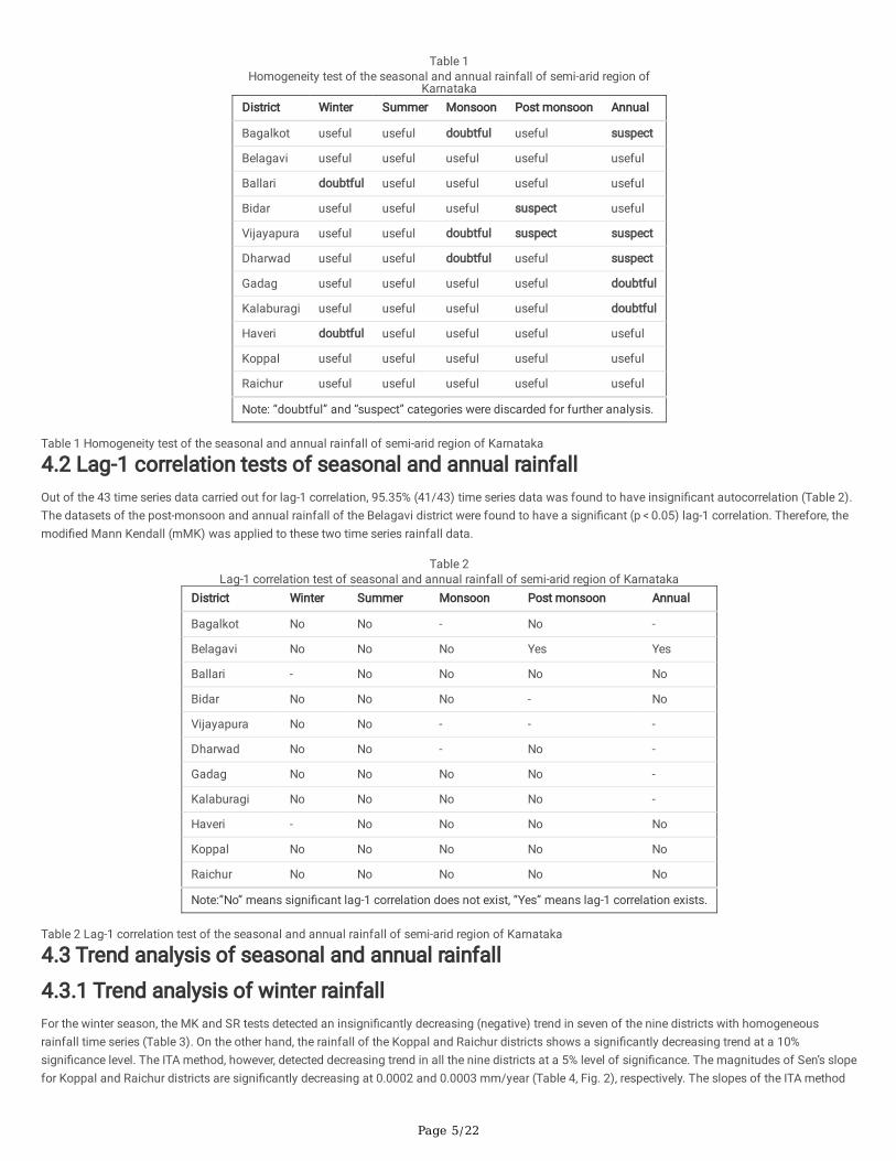
4.1 Homogeneity tests of seasonal and annual rainfallAll the 55 time series of the 11 districts were subject to four homogeneity tests, as shown in Table 1. For the winter season, the rainfall time series data ofthe Ballari and Haveri districts were doubtful. However, all the time series data of the summer season were in the useful category. The time series data ofBagalkot, Vijayapura, and Dharwad districts were doubtful for monsoon season. On the other hand, for the post-monsoon season, the rainfall of the Bidarand Vijayapura districts was identi�ed to be in the suspect category. Also, the annual rainfall of Bagalkot, Vijayapura, and Dharwad fall into the suspectcategory. The rainfall of Bagalkot, Gadag, and Kalaburagi districts falls into the doubtful category. All the rainfall time series falling in the doubtful orsuspect category were discarded from further analysis. Hence, 78.18% (43/55) of the total time series data were used for further analysis.

Page 5/22

Table 1Homogeneity test of the seasonal and annual rainfall of semi-arid region of

KarnatakaDistrict Winter Summer Monsoon Post monsoon Annual

Bagalkot useful useful doubtful useful suspect

Belagavi useful useful useful useful useful

Ballari doubtful useful useful useful useful

Bidar useful useful useful suspect useful

Vijayapura useful useful doubtful suspect suspect

Dharwad useful useful doubtful useful suspect

Gadag useful useful useful useful doubtful

Kalaburagi useful useful useful useful doubtful

Haveri doubtful useful useful useful useful

Koppal useful useful useful useful useful

Raichur useful useful useful useful useful

Note: “doubtful” and “suspect” categories were discarded for further analysis.

Table 1 Homogeneity test of the seasonal and annual rainfall of semi-arid region of Karnataka

4.2 Lag-1 correlation tests of seasonal and annual rainfallOut of the 43 time series data carried out for lag-1 correlation, 95.35% (41/43) time series data was found to have insigni�cant autocorrelation (Table 2).The datasets of the post-monsoon and annual rainfall of the Belagavi district were found to have a signi�cant (p < 0.05) lag-1 correlation. Therefore, themodi�ed Mann Kendall (mMK) was applied to these two time series rainfall data.

Table 2Lag-1 correlation test of seasonal and annual rainfall of semi-arid region of Karnataka

District Winter Summer Monsoon Post monsoon Annual

Bagalkot No No - No -

Belagavi No No No Yes Yes

Ballari - No No No No

Bidar No No No - No

Vijayapura No No - - -

Dharwad No No - No -

Gadag No No No No -

Kalaburagi No No No No -

Haveri - No No No No

Koppal No No No No No

Raichur No No No No No

Note:”No” means signi�cant lag-1 correlation does not exist, “Yes” means lag-1 correlation exists.

Table 2 Lag-1 correlation test of the seasonal and annual rainfall of semi-arid region of Karnataka

4.3 Trend analysis of seasonal and annual rainfall

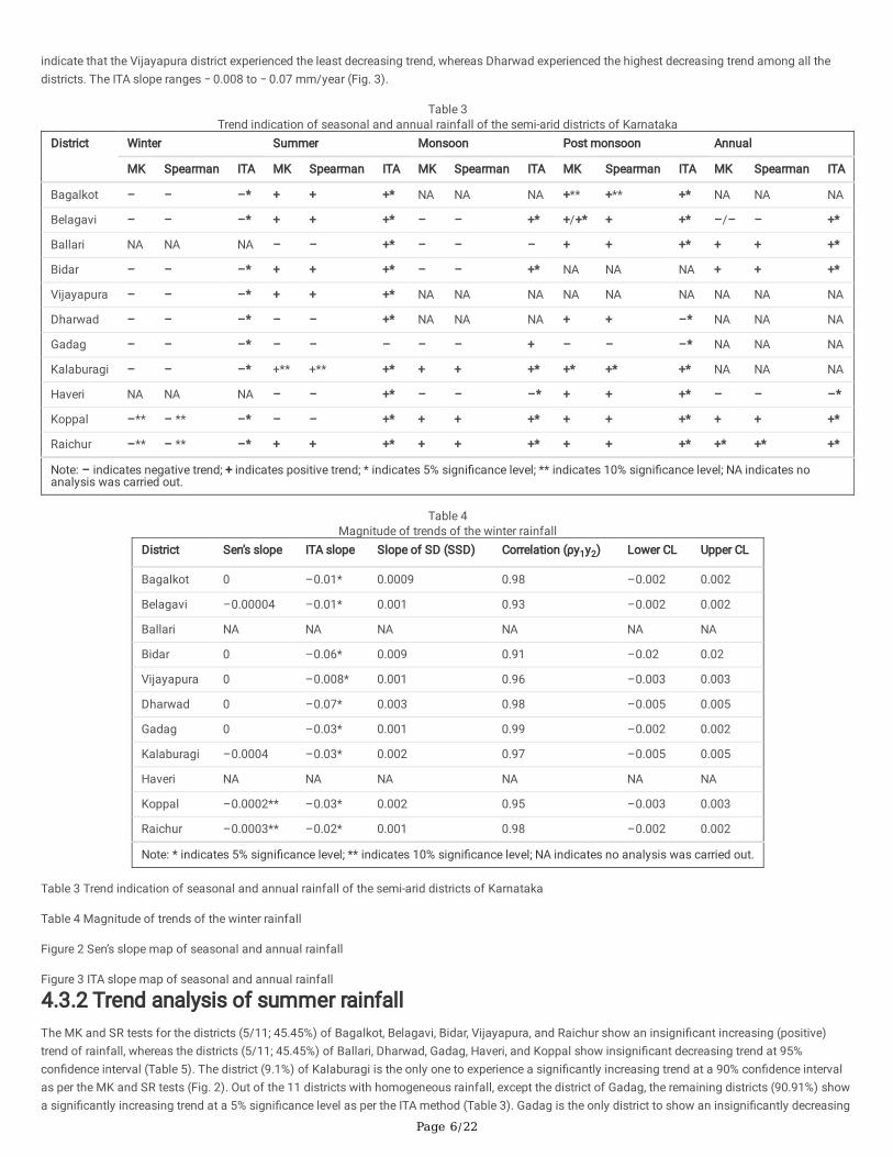
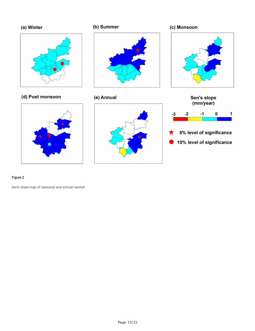
4.3.1 Trend analysis of winter rainfallFor the winter season, the MK and SR tests detected an insigni�cantly decreasing (negative) trend in seven of the nine districts with homogeneousrainfall time series (Table 3). On the other hand, the rainfall of the Koppal and Raichur districts shows a signi�cantly decreasing trend at a 10%signi�cance level. The ITA method, however, detected decreasing trend in all the nine districts at a 5% level of signi�cance. The magnitudes of Sen’s slopefor Koppal and Raichur districts are signi�cantly decreasing at 0.0002 and 0.0003 mm/year (Table 4, Fig. 2), respectively. The slopes of the ITA method

Page 6/22

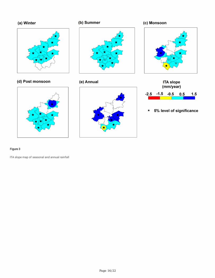
indicate that the Vijayapura district experienced the least decreasing trend, whereas Dharwad experienced the highest decreasing trend among all thedistricts. The ITA slope ranges − 0.008 to − 0.07 mm/year (Fig. 3).

Table 3Trend indication of seasonal and annual rainfall of the semi-arid districts of Karnataka

District Winter Summer Monsoon Post monsoon Annual

MK Spearman ITA MK Spearman ITA MK Spearman ITA MK Spearman ITA MK Spearman ITA

Bagalkot – – –* + + +* NA NA NA +** +** +* NA NA NA

Belagavi – – –* + + +* – – +* +/+* + +* –/– – +*

Ballari NA NA NA – – +* – – – + + +* + + +*

Bidar – – –* + + +* – – +* NA NA NA + + +*

Vijayapura – – –* + + +* NA NA NA NA NA NA NA NA NA

Dharwad – – –* – – +* NA NA NA + + –* NA NA NA

Gadag – – –* – – – – – + – – –* NA NA NA

Kalaburagi – – –* +** +** +* + + +* +* +* +* NA NA NA

Haveri NA NA NA – – +* – – –* + + +* – – –*

Koppal –** – ** –* – – +* + + +* + + +* + + +*

Raichur –** – ** –* + + +* + + +* + + +* +* +* +*

Note: – indicates negative trend; + indicates positive trend; * indicates 5% signi�cance level; ** indicates 10% signi�cance level; NA indicates noanalysis was carried out.

Table 4Magnitude of trends of the winter rainfall

District Sen’s slope ITA slope Slope of SD (SSD) Correlation (ρy1y2) Lower CL Upper CL

Bagalkot 0 –0.01* 0.0009 0.98 –0.002 0.002

Belagavi –0.00004 –0.01* 0.001 0.93 –0.002 0.002

Ballari NA NA NA NA NA NA

Bidar 0 –0.06* 0.009 0.91 –0.02 0.02

Vijayapura 0 –0.008* 0.001 0.96 –0.003 0.003

Dharwad 0 –0.07* 0.003 0.98 –0.005 0.005

Gadag 0 –0.03* 0.001 0.99 –0.002 0.002

Kalaburagi –0.0004 –0.03* 0.002 0.97 –0.005 0.005

Haveri NA NA NA NA NA NA

Koppal –0.0002** –0.03* 0.002 0.95 –0.003 0.003

Raichur –0.0003** –0.02* 0.001 0.98 –0.002 0.002

Note: * indicates 5% signi�cance level; ** indicates 10% signi�cance level; NA indicates no analysis was carried out.

Table 3 Trend indication of seasonal and annual rainfall of the semi-arid districts of Karnataka

Table 4 Magnitude of trends of the winter rainfall

Figure 2 Sen’s slope map of seasonal and annual rainfall

Figure 3 ITA slope map of seasonal and annual rainfall

4.3.2 Trend analysis of summer rainfallThe MK and SR tests for the districts (5/11; 45.45%) of Bagalkot, Belagavi, Bidar, Vijayapura, and Raichur show an insigni�cant increasing (positive)trend of rainfall, whereas the districts (5/11; 45.45%) of Ballari, Dharwad, Gadag, Haveri, and Koppal show insigni�cant decreasing trend at 95%con�dence interval (Table 5). The district (9.1%) of Kalaburagi is the only one to experience a signi�cantly increasing trend at a 90% con�dence intervalas per the MK and SR tests (Fig. 2). Out of the 11 districts with homogeneous rainfall, except the district of Gadag, the remaining districts (90.91%) showa signi�cantly increasing trend at a 5% signi�cance level as per the ITA method (Table 3). Gadag is the only district to show an insigni�cantly decreasing

Page 7/22

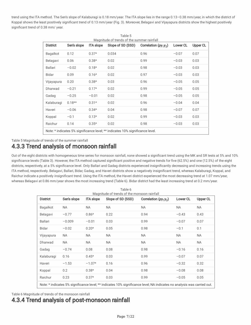
trend using the ITA method. The Sen’s slope of Kalaburagi is 0.18 mm/year. The ITA slope lies in the range 0.13–0.38 mm/year, in which the district ofKoppal shows the least positively signi�cant trend of 0.13 mm/year (Fig. 3). Moreover, Belagavi and Vijayapura districts show the highest positivelysigni�cant trend of 0.38 mm/ year.

Table 5Magnitude of trends of the summer rainfall

District Sen’s slope ITA slope Slope of SD (SSD) Correlation (ρy1y2) Lower CL Upper CL

Bagalkot 0.12 0.37* 0.034 0.96 –0.07 0.07

Belagavi 0.06 0.38* 0.02 0.99 –0.03 0.03

Ballari –0.02 0.18* 0.02 0.98 –0.03 0.03

Bidar 0.09 0.16* 0.02 0.97 –0.03 0.03

Vijayapura 0.20 0.38* 0.03 0.96 –0.05 0.05

Dharwad –0.21 0.17* 0.02 0.99 –0.05 0.05

Gadag –0.25 –0.01 0.02 0.98 –0.05 0.05

Kalaburagi 0.18** 0.31* 0.02 0.96 –0.04 0.04

Haveri –0.06 0.34* 0.04 0.98 –0.07 0.07

Koppal –0.1 0.13* 0.02 0.99 –0.03 0.03

Raichur 0.14 0.35* 0.02 0.98 –0.03 0.03

Note: * indicates 5% signi�cance level; ** indicates 10% signi�cance level.

Table 5 Magnitude of trends of the summer rainfall

4.3.3 Trend analysis of monsoon rainfallOut of the eight districts with homogeneous time series for monsoon rainfall, none showed a signi�cant trend using the MK and SR tests at 5% and 10%signi�cance levels (Table 3). However, the ITA method captured signi�cant positive and negative trends for �ve (62.5%) and one (12.5%) of the eightdistricts, respectively, at a 5% signi�cance level. Only Ballari and Gadag districts experienced insigni�cantly decreasing and increasing trends using theITA method, respectively. Belagavi, Ballari, Bidar, Gadag, and Haveri districts show a negatively insigni�cant trend, whereas Kalaburagi, Koppal, andRaichur indicate a positively insigni�cant trend. Using the ITA method, the Haveri district experienced the most decreasing trend at 1.07 mm/year,whereas Belagavi at 0.86 mm/year shows the most increasing trend (Table 6). Bidar district had the least increasing trend at 0.2 mm/year.

Table 6Magnitude of trends of the monsoon rainfall

District Sen’s slope ITA slope Slope of SD (SSD) Correlation (ρy1y2) Lower CL Upper CL

Bagalkot NA NA NA NA NA NA

Belagavi –0.77 0.86* 0.22 0.94 –0.43 0.43

Ballari –0.009 –0.01 0.03 0.99 –0.07 0.07

Bidar –0.02 0.20* 0.05 0.98 –0.1 0.1

Vijayapura NA NA NA NA NA NA

Dharwad NA NA NA NA NA NA

Gadag –0.74 0.08 0.08 0.98 –0.16 0.16

Kalaburagi 0.16 0.45* 0.03 0.99 –0.07 0.07

Haveri –1.53 –1.07* 0.16 0.96 –0.32 0.32

Koppal 0.2 0.38* 0.04 0.98 –0.08 0.08

Raichur 0.23 0.37* 0.03 0.99 –0.05 0.05

Note: * indicates 5% signi�cance level; ** indicates 10% signi�cance level; NA indicates no analysis was carried out.

Table 6 Magnitude of trends of the monsoon rainfall

4.3.4 Trend analysis of post-monsoon rainfall

Page 8/22

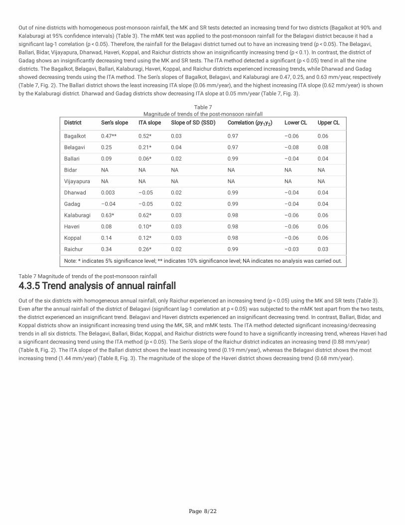
Out of nine districts with homogeneous post-monsoon rainfall, the MK and SR tests detected an increasing trend for two districts (Bagalkot at 90% andKalaburagi at 95% con�dence intervals) (Table 3). The mMK test was applied to the post-monsoon rainfall for the Belagavi district because it had asigni�cant lag-1 correlation (p < 0.05). Therefore, the rainfall for the Belagavi district turned out to have an increasing trend (p < 0.05). The Belagavi,Ballari, Bidar, Vijayapura, Dharwad, Haveri, Koppal, and Raichur districts show an insigni�cantly increasing trend (p < 0.1). In contrast, the district ofGadag shows an insigni�cantly decreasing trend using the MK and SR tests. The ITA method detected a signi�cant (p < 0.05) trend in all the ninedistricts. The Bagalkot, Belagavi, Ballari, Kalaburagi, Haveri, Koppal, and Raichur districts experienced increasing trends, while Dharwad and Gadagshowed decreasing trends using the ITA method. The Sen’s slopes of Bagalkot, Belagavi, and Kalaburagi are 0.47, 0.25, and 0.63 mm/year, respectively(Table 7, Fig. 2). The Ballari district shows the least increasing ITA slope (0.06 mm/year), and the highest increasing ITA slope (0.62 mm/year) is shownby the Kalaburagi district. Dharwad and Gadag districts show decreasing ITA slope at 0.05 mm/year (Table 7, Fig. 3).

Table 7Magnitude of trends of the post-monsoon rainfall

District Sen’s slope ITA slope Slope of SD (SSD) Correlation (ρy1y2) Lower CL Upper CL

Bagalkot 0.47** 0.52* 0.03 0.97 –0.06 0.06

Belagavi 0.25 0.21* 0.04 0.97 –0.08 0.08

Ballari 0.09 0.06* 0.02 0.99 –0.04 0.04

Bidar NA NA NA NA NA NA

Vijayapura NA NA NA NA NA NA

Dharwad 0.003 –0.05 0.02 0.99 –0.04 0.04

Gadag –0.04 –0.05 0.02 0.99 –0.04 0.04

Kalaburagi 0.63* 0.62* 0.03 0.98 –0.06 0.06

Haveri 0.08 0.10* 0.03 0.98 –0.06 0.06

Koppal 0.14 0.12* 0.03 0.98 –0.06 0.06

Raichur 0.34 0.26* 0.02 0.99 –0.03 0.03

Note: * indicates 5% signi�cance level; ** indicates 10% signi�cance level; NA indicates no analysis was carried out.

Table 7 Magnitude of trends of the post-monsoon rainfall

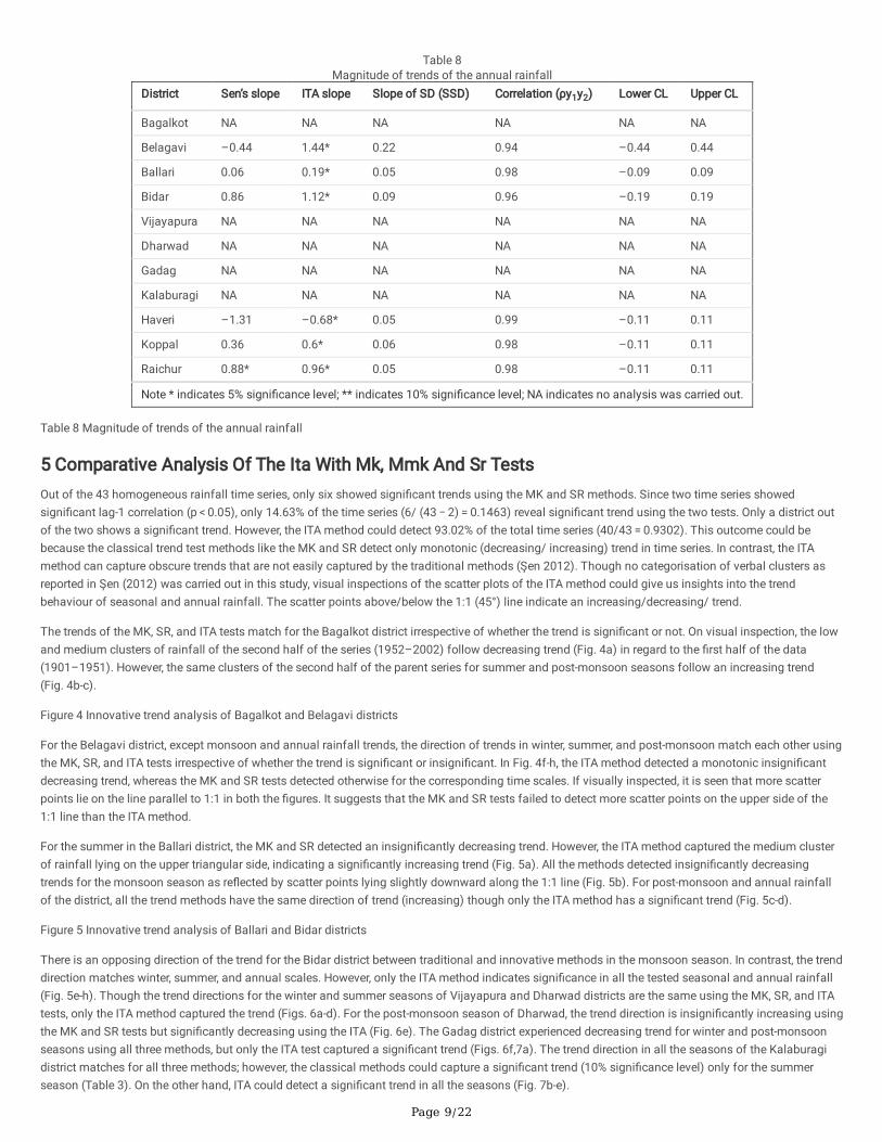
4.3.5 Trend analysis of annual rainfallOut of the six districts with homogeneous annual rainfall, only Raichur experienced an increasing trend (p < 0.05) using the MK and SR tests (Table 3).Even after the annual rainfall of the district of Belagavi (signi�cant lag-1 correlation at p < 0.05) was subjected to the mMK test apart from the two tests,the district experienced an insigni�cant trend. Belagavi and Haveri districts experienced an insigni�cant decreasing trend. In contrast, Ballari, Bidar, andKoppal districts show an insigni�cant increasing trend using the MK, SR, and mMK tests. The ITA method detected signi�cant increasing/decreasingtrends in all six districts. The Belagavi, Ballari, Bidar, Koppal, and Raichur districts were found to have a signi�cantly increasing trend, whereas Haveri hada signi�cant decreasing trend using the ITA method (p < 0.05). The Sen’s slope of the Raichur district indicates an increasing trend (0.88 mm/year)(Table 8, Fig. 2). The ITA slope of the Ballari district shows the least increasing trend (0.19 mm/year), whereas the Belagavi district shows the mostincreasing trend (1.44 mm/year) (Table 8, Fig. 3). The magnitude of the slope of the Haveri district shows decreasing trend (0.68 mm/year).

Page 9/22

Table 8Magnitude of trends of the annual rainfall

District Sen’s slope ITA slope Slope of SD (SSD) Correlation (ρy1y2) Lower CL Upper CL

Bagalkot NA NA NA NA NA NA

Belagavi –0.44 1.44* 0.22 0.94 –0.44 0.44

Ballari 0.06 0.19* 0.05 0.98 –0.09 0.09

Bidar 0.86 1.12* 0.09 0.96 –0.19 0.19

Vijayapura NA NA NA NA NA NA

Dharwad NA NA NA NA NA NA

Gadag NA NA NA NA NA NA

Kalaburagi NA NA NA NA NA NA

Haveri –1.31 –0.68* 0.05 0.99 –0.11 0.11

Koppal 0.36 0.6* 0.06 0.98 –0.11 0.11

Raichur 0.88* 0.96* 0.05 0.98 –0.11 0.11

Note * indicates 5% signi�cance level; ** indicates 10% signi�cance level; NA indicates no analysis was carried out.

Table 8 Magnitude of trends of the annual rainfall

5 Comparative Analysis Of The Ita With Mk, Mmk And Sr TestsOut of the 43 homogeneous rainfall time series, only six showed signi�cant trends using the MK and SR methods. Since two time series showedsigni�cant lag-1 correlation (p < 0.05), only 14.63% of the time series (6/ (43 − 2) = 0.1463) reveal signi�cant trend using the two tests. Only a district outof the two shows a signi�cant trend. However, the ITA method could detect 93.02% of the total time series (40/43 = 0.9302). This outcome could bebecause the classical trend test methods like the MK and SR detect only monotonic (decreasing/ increasing) trend in time series. In contrast, the ITAmethod can capture obscure trends that are not easily captured by the traditional methods (Şen 2012). Though no categorisation of verbal clusters asreported in Şen (2012) was carried out in this study, visual inspections of the scatter plots of the ITA method could give us insights into the trendbehaviour of seasonal and annual rainfall. The scatter points above/below the 1:1 (45°) line indicate an increasing/decreasing/ trend.

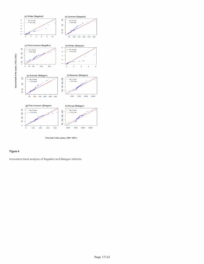
The trends of the MK, SR, and ITA tests match for the Bagalkot district irrespective of whether the trend is signi�cant or not. On visual inspection, the lowand medium clusters of rainfall of the second half of the series (1952–2002) follow decreasing trend (Fig. 4a) in regard to the �rst half of the data(1901–1951). However, the same clusters of the second half of the parent series for summer and post-monsoon seasons follow an increasing trend(Fig. 4b-c).

Figure 4 Innovative trend analysis of Bagalkot and Belagavi districts

For the Belagavi district, except monsoon and annual rainfall trends, the direction of trends in winter, summer, and post-monsoon match each other usingthe MK, SR, and ITA tests irrespective of whether the trend is signi�cant or insigni�cant. In Fig. 4f-h, the ITA method detected a monotonic insigni�cantdecreasing trend, whereas the MK and SR tests detected otherwise for the corresponding time scales. If visually inspected, it is seen that more scatterpoints lie on the line parallel to 1:1 in both the �gures. It suggests that the MK and SR tests failed to detect more scatter points on the upper side of the1:1 line than the ITA method.

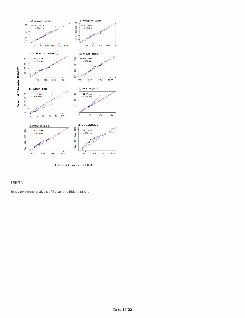
For the summer in the Ballari district, the MK and SR detected an insigni�cantly decreasing trend. However, the ITA method captured the medium clusterof rainfall lying on the upper triangular side, indicating a signi�cantly increasing trend (Fig. 5a). All the methods detected insigni�cantly decreasingtrends for the monsoon season as re�ected by scatter points lying slightly downward along the 1:1 line (Fig. 5b). For post-monsoon and annual rainfallof the district, all the trend methods have the same direction of trend (increasing) though only the ITA method has a signi�cant trend (Fig. 5c-d).

Figure 5 Innovative trend analysis of Ballari and Bidar districts

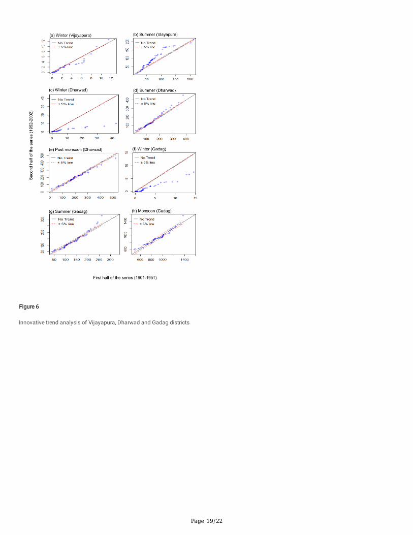
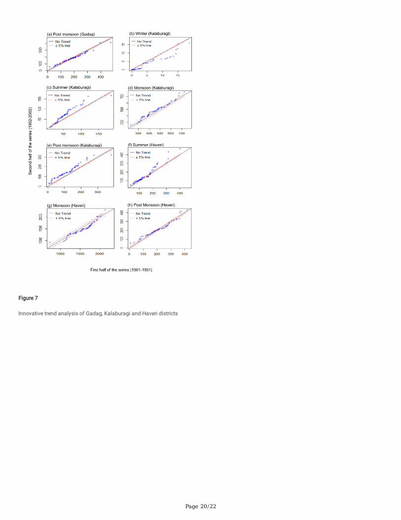
There is an opposing direction of the trend for the Bidar district between traditional and innovative methods in the monsoon season. In contrast, the trenddirection matches winter, summer, and annual scales. However, only the ITA method indicates signi�cance in all the tested seasonal and annual rainfall(Fig. 5e-h). Though the trend directions for the winter and summer seasons of Vijayapura and Dharwad districts are the same using the MK, SR, and ITAtests, only the ITA method captured the trend (Figs. 6a-d). For the post-monsoon season of Dharwad, the trend direction is insigni�cantly increasing usingthe MK and SR tests but signi�cantly decreasing using the ITA (Fig. 6e). The Gadag district experienced decreasing trend for winter and post-monsoonseasons using all three methods, but only the ITA test captured a signi�cant trend (Figs. 6f,7a). The trend direction in all the seasons of the Kalaburagidistrict matches for all three methods; however, the classical methods could capture a signi�cant trend (10% signi�cance level) only for the summerseason (Table 3). On the other hand, ITA could detect a signi�cant trend in all the seasons (Fig. 7b-e).

Page 10/22

Figure 6 Innovative trend analysis of Vijayapura, Dharwad and Gadag districts

Figure 7 Innovative trend analysis of Gadag, Kalaburagi and Haveri districts

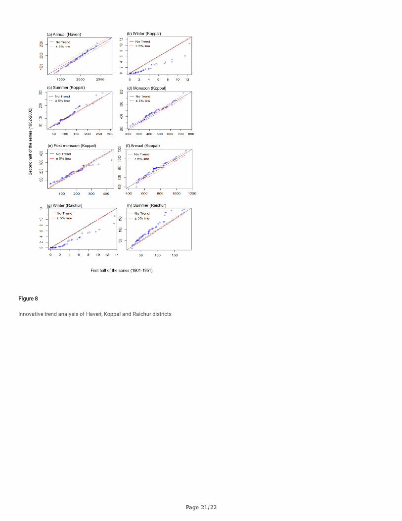
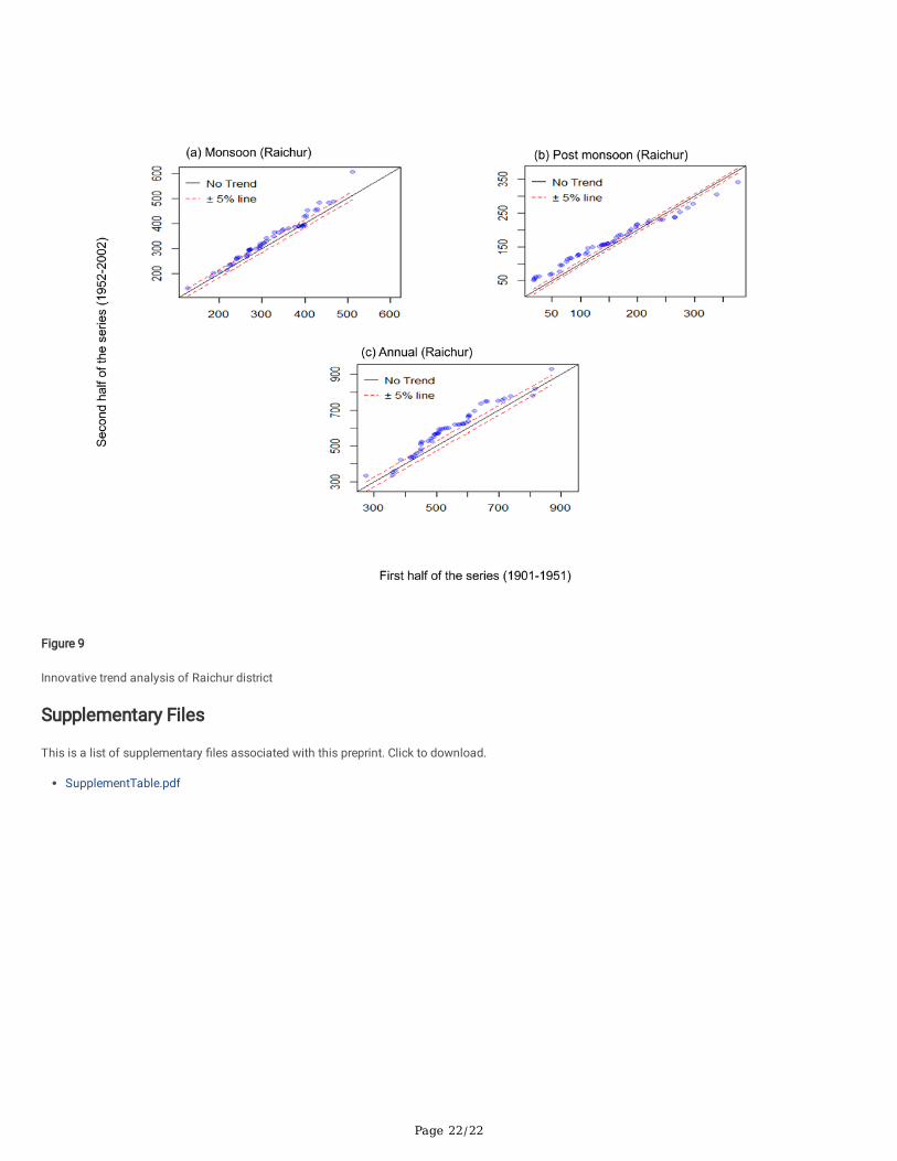
Except for the summer season in the Haveri district, the trend direction of monsoon, post-monsoon, and annual rainfall is the same. As with otherdistricts, ITA captured a signi�cant trend for all the mentioned seasons and annually (Figs. 7f-h,8a). For the Koppal district, except for the summer seasontrend, all other seasons and annual rainfall showed the same trend direction using all three methods. The two traditional methods could capture asigni�cant trend in the winter season, whereas the ITA captured a signi�cant trend in all the seasons (Fig. 8b-f). For the Raichur district, the trend directionmatches for all the seasons and annual scale. The trend is signi�cant for winter and annual rainfall using the MK and SR tests, but the ITA could detect asigni�cant trend for all seasonal and annual scales (Figs. 8g-9c). The comparisons carried out for all seasonal and annual rainfall of the 11 districtsusing the ITA and traditional methods reveal that the ITA approach was indeed able to capture the monotonic trends detected by the traditional methodsand the obscure trends. The outcome of the current study corroborates with the �ndings reported in recent literature (Marak et al. 2020; Singh et al.2021b, a).

Figure 8 Innovative trend analysis of Haveri, Koppal and Raichur districts

Figure 9 Innovative trend analysis of Raichur district

6 ConclusionsIn this study, trend analysis was investigated using the MK, mMK, SR, and the ITA methods for the seasonal and annual rainfall of 11 semi-arid districtsin Karnataka for 102 years (1901–2002) of data. Only 78.18% (43/55) of the total time series data were homogeneous based on a two-step approachthat involved four statistical methods and classi�cation of the methods into three categories. Out of the 43 homogeneous time series data, 95.35%(41/43) time series data were found to have insigni�cant autocorrelation. The post-monsoon and annual rainfall of the Belagavi district were found tohave a signi�cant (p < 0.05) lag-1 correlation; however, the mMK test showed an increasing trend for the post-monsoon season only. The MK and SR testsdetected 14.63% of the time series (6/ (43 − 2) = 0.1463) as a signi�cant trend. However, the ITA method could detect 93.02% (40/43 = 0.9302) of the totaltime series. The MK and SR tests could capture a signi�cant trend for the winter season in Koppal and Raichur districts. The two tests could detectsigni�cant trend only in the Kalaburagi district for the summer season. No trend could be captured for the monsoon season. The signi�cant trend inBagalkot and Kalaburagi districts could be captured for the post-monsoon season. The tests could detect a signi�cant trend in the Raichur district forannual rainfall; however, the ITA captured a signi�cant trend for all the seasons in most districts.

DeclarationsData availability  

The datasets generated during and/or analysed during the current study are available in the India water portalrepository, http://www.indiawaterportal.org/metdata

Compliance with Ethical Standards

The authors declare that they have no known con�ict of interest.

References1. Abghari H, Tabari H, Hosseinzadeh Talaee P (2013) River �ow trends in the west of Iran during the past 40years: Impact of precipitation variability.

Glob Planet Change 101:52–60. https://doi.org/10.1016/j.gloplacha.2012.12.003

2. Aher MC, Yadav SM (2021) Assessment of rainfall trend and variability of semi-arid regions of Upper and Middle Godavari basin, India. J Water ClimChang 12:3992–4006. https://doi.org/10.2166/wcc.2021.044

3. Ahmed N, Wang G, Booij MJ et al (2021) Changes in monthly stream�ow in the Hindukush–Karakoram–Himalaya Region of Pakistan usinginnovative polygon trend analysis. Stoch Environ Res Risk Assess. https://doi.org/10.1007/s00477-021-02067-0

4. Akçay F, Kankal M, Şan M (2021) Innovative approaches to the trend assessment of stream�ows in the eastern Black Sea basin, Turkey. Hydrol Sci J.https://doi.org/10.1080/02626667.2021.1998509

5. Alexandersson H (1986) A homogeneity test applied to precipitation data. J Climatol 6:661–675. https://doi.org/10.1002/joc.3370060607

�. Ay M (2022) Trend of minimum monthly precipitation for the East Anatolia region in Turkey. Theor Appl Climatol. https://doi.org/10.1007/s00704-022-03947-3

7. Behrang Manesh M, Khosravi H, Heydari Alamdarloo E et al (2019) Linkage of agricultural drought with meteorological drought in different climatesof Iran. Theor Appl Climatol 138:1025–1033. https://doi.org/10.1007/s00704-019-02878-w

�. Buishand TA (1982) Some methods for testing the homogeneity of rainfall records. J Hydrol 58:11–27. https://doi.org/10.1016/0022-1694(82)90066-X

Page 11/22

9. Ceribasi G, Ceyhunlu AI (2021) Analysis of total monthly precipitation of Susurluk Basin in Turkey using innovative polygon trend analysis method. JWater Clim Chang 12:1532–1543. https://doi.org/10.2166/wcc.2020.253

10. Ceribasi G, Ceyhunlu AI, Ahmed N (2021) Innovative trend pivot analysis method (ITPAM): a case study for precipitation data of Susurluk Basin inTurkey. Acta Geophys 69:1465–1480. https://doi.org/10.1007/s11600-021-00605-6

11. Chatterjee S, Khan A, Akbari H, Wang Y (2016) Monotonic trends in spatio-temporal distribution and concentration of monsoon precipitation (1901–2002), West Bengal, India. Atmos Res 182:54–75. https://doi.org/10.1016/j.atmosres.2016.07.010

12. Danandeh Mehr A, Hrnjica B, Bonacci O, Torabi Haghighi A (2021) Innovative and successive average trend analysis of temperature and precipitationin Osijek, Croatia. Theor Appl Climatol 145:875–890. https://doi.org/10.1007/s00704-021-03672-3

13. Daniel WW (1990) Applied nonparametric statistics, 2nd edn. Duxbury, Paci�c Grove, CA

14. Doaemo W, Wuest L, Athikalam PT et al (2022) Rainfall characterization of the Bumbu watershed, Papua New Guinea. Theor Appl Climatol147:127–141. https://doi.org/10.1007/s00704-021-03808-5

15. Fekete A, Sandholz S (2021) Here Comes the Flood, but Not Failure? Lessons to Learn after the Heavy Rain and Pluvial Floods in Germany 2021.Water 13:3016. https://doi.org/10.3390/w13213016

1�. Formetta G, Capparelli G, David O et al (2016) Integration of a Three-Dimensional Process-Based Hydrological Model into the Object ModelingSystem. Water 8:12. https://doi.org/10.3390/w8010012

17. Gado TA, El-Hagrsy RM, Rashwan IMH (2019) Spatial and temporal rainfall changes in Egypt. Environ Sci Pollut Res 26:28228–28242.https://doi.org/10.1007/s11356-019-06039-4

1�. Gajbhiye S, Meshram C, Singh SK et al (2016) Precipitation trend analysis of Sindh River basin, India, from 102-year record (1901–2002). Atmos SciLett 17:71–77. https://doi.org/10.1002/asl.602

19. Gocic M, Trajkovic S (2013) Analysis of precipitation and drought data in Serbia over the period 1980–2010. J Hydrol 494:32–42.https://doi.org/10.1016/j.jhydrol.2013.04.044

20. Goyal MK (2014) Statistical Analysis of Long Term Trends of Rainfall During 1901–2002 at Assam, India. Water Resour Manag 28:1501–1515.https://doi.org/10.1007/s11269-014-0529-y

21. Güçlü YS (2018a) Alternative Trend Analysis: Half Time Series Methodology. Water Resour Manag 32:2489–2504. https://doi.org/10.1007/s11269-018-1942-4

22. Güçlü YS (2018b) Multiple Şen-innovative trend analyses and partial Mann-Kendall test. J Hydrol 566:685–704.https://doi.org/10.1016/j.jhydrol.2018.09.034

23. Güçlü YS, Şişman E, Dabanlı İ (2020) Innovative triangular trend analysis. Arab J Geosci 13:27. https://doi.org/10.1007/s12517-019-5048-y

24. Güner Bacanli Ü (2017) Trend analysis of precipitation and drought in the Aegean region, Turkey. Meteorol Appl 24:239–249.https://doi.org/10.1002/met.1622

25. Gupta A, Sawant CP, Rao KVR, Sarangi A (2021) Results of century analysis of rainfall and temperature trends and its impact on agricultureproduction in Bundelkhand region of Central India. MAUSAM 72:473–488. https://doi.org/10.54302/mausam.v72i2.608

2�. Hajani E, Rahman A, Ishak E (2017) Trends in extreme rainfall in the state of New South Wales, Australia. Hydrol Sci J 62:2160–2174.https://doi.org/10.1080/02626667.2017.1368520

27. Hao Z, Hao F, Singh VP et al (2016) Probabilistic prediction of hydrologic drought using a conditional probability approach based on the meta-Gaussian model. J Hydrol 542:772–780. https://doi.org/10.1016/j.jhydrol.2016.09.048

2�. Harka AE, Jilo NB, Behulu F (2021) Spatial-temporal rainfall trend and variability assessment in the Upper Wabe Shebelle River Basin, Ethiopia:Application of innovative trend analysis method. J Hydrol Reg Stud 37:100915. https://doi.org/10.1016/j.ejrh.2021.100915

29. Hırca T, Eryılmaz Türkkan G, Niazkar M (2022) Applications of innovative polygonal trend analyses to precipitation series of Eastern Black Sea Basin,Turkey. Theor Appl Climatol 147:651–667. https://doi.org/10.1007/s00704-021-03837-0

30. Jameel Y, Stahl M, Ahmad S et al (2020) India needs an effective �ood policy. Sci (80-) 369:1575–1575. https://doi.org/10.1126/science.abe2962

31. Jayasree V, Venkatesh B (2015) Analysis of Rainfall in Assessing the Drought in Semi-arid Region of Karnataka State, India. Water Resour Manag29:5613–5630. https://doi.org/10.1007/s11269-015-1137-1

32. Jha VB, Gujrati A, Singh RP (2021) Complex network theoretic assessment of precipitation-driven meteorological drought in India: Past and future.Int J Climatol. https://doi.org/10.1002/joc.7397

33. Kalra A, Ahmad S (2011) Evaluating changes and estimating seasonal precipitation for the Colorado River Basin using a stochastic nonparametricdisaggregation technique. Water Resour Res 47. https://doi.org/10.1029/2010WR009118

34. Kaur S, Diwakar SK, Das AK (2021) Long term rainfall trend over meteorological sub divisions and districts of India. MAUSAM 68:439–450.https://doi.org/10.54302/mausam.v68i3.676

35. Kendall MG (1938) A New Measure of Rank Ccorrelation. Biometrika 30:81–93. https://doi.org/10.1093/biomet/30.1-2.81

3�. Kumar V, Jain SK, Singh Y (2010) Analysis of long-term rainfall trends in India. Hydrol Sci J 55:484–496.https://doi.org/10.1080/02626667.2010.481373

Page 12/22

37. Machiwal D, Gupta A, Jha MK, Kamble T (2019) Analysis of trend in temperature and rainfall time series of an Indian arid region: comparativeevaluation of salient techniques. Theor Appl Climatol 136:301–320. https://doi.org/10.1007/s00704-018-2487-4

3�. Mahato LL, Kumar M, Suryavanshi S et al (2021) Statistical investigation of long-term meteorological data to understand the variability in climate: acase study of Jharkhand, India. Environ Dev Sustain 23:16981–17002. https://doi.org/10.1007/s10668-021-01374-4

39. Mallick J, Talukdar S, Almesfer MK et al (2021) Identi�cation of rainfall homogenous regions in Saudi Arabia for experimenting and improving trenddetection techniques. Environ Sci Pollut Res. https://doi.org/10.1007/s11356-021-17609-w

40. Mann HB (1945) Nonparametric Tests Against Trend. Econometrica 13:245. https://doi.org/10.2307/1907187

41. Marak JDK, Sarma AK, Bhattacharjya RK (2020) Innovative trend analysis of spatial and temporal rainfall variations in Umiam and Umtruwatersheds in Meghalaya, India. Theor Appl Climatol 142:1397–1412. https://doi.org/10.1007/s00704-020-03383-1

42. Meena HM, Machiwal D, Santra P et al (2019) Trends and homogeneity of monthly, seasonal, and annual rainfall over arid region of Rajasthan, India.Theor Appl Climatol 136:795–811. https://doi.org/10.1007/s00704-018-2510-9

43. Mehta D, Yadav SM (2021) An analysis of rainfall variability and drought over Barmer District of Rajasthan, Northwest India. Water Supply 21:2505–2517. https://doi.org/10.2166/ws.2021.053

44. Meshram SG, Singh VP, Meshram C (2017) Long-term trend and variability of precipitation in Chhattisgarh State, India. Theor Appl Climatol129:729–744. https://doi.org/10.1007/s00704-016-1804-z

45. Mishra AK, Nagaraju V (2019) Space-based monitoring of severe �ooding of a southern state in India during south-west monsoon season of 2018.Nat Hazards 97:949–953. https://doi.org/10.1007/s11069-019-03673-6

4�. Mishra V, Thirumalai K, Jain S, Aadhar S (2021) Unprecedented drought in South India and recent water scarcity. Environ Res Lett 16:054007.https://doi.org/10.1088/1748-9326/abf289

47. Muthuvel D, Mahesha A (2021) Spatiotemporal Analysis of Compound Agrometeorological Drought and Hot Events in India Using a StandardizedIndex. J Hydrol Eng 26. https://doi.org/10.1061/(ASCE)HE.1943-5584.0002101. :(ASCE)HE.1943-5584.0002101

4�. Nengzouzam G, Hodam S, Bandyopadhyay A, Bhadra A (2020) Spatial and temporal trends in high resolution gridded rainfall data over India. J EarthSyst Sci 129:232. https://doi.org/10.1007/s12040-020-01494-x

49. Nikzad Tehrani E, Sahour H, Booij MJ (2019) Trend analysis of hydro-climatic variables in the north of Iran. Theor Appl Climatol 136:85–97.https://doi.org/10.1007/s00704-018-2470-0

50. Pandey BK, Khare D (2018) Identi�cation of trend in long term precipitation and reference evapotranspiration over Narmada river basin (India). GlobPlanet Change 161:172–182. https://doi.org/10.1016/j.gloplacha.2017.12.017

51. Patakamuri SK, Das B (2019) Trendchange: innovative trend analysis and time-series change point analysis.R package version1.1

52. Patakamuri SK, O’Brien NM (2020) Modi�ed versions of Mann Kendall and Spearman’s Rho trend tests.R Packag version1

53. Pettitt AN (1979) A Non-Parametric Approach to the Change-Point Problem. Appl Stat 28:126. https://doi.org/10.2307/2346729

54. Phuong DND, Huyen NT, Liem ND et al (2022) On the use of an innovative trend analysis methodology for temporal trend identi�cation in extremerainfall indices over the Central Highlands, Vietnam. Theor Appl Climatol 147:835–852. https://doi.org/10.1007/s00704-021-03842-3

55. Praveen B, Talukdar S, Shahfahad et al (2020) Analyzing trend and forecasting of rainfall changes in India using non-parametrical and machinelearning approaches. Sci Rep 10:10342. https://doi.org/10.1038/s41598-020-67228-7

5�. Raja NB, Aydin O (2019) Trend analysis of annual precipitation of Mauritius for the period 1981–2010. Meteorol Atmos Phys 131:789–805.https://doi.org/10.1007/s00703-018-0604-7

57. Saini A, Sahu N (2021) Decoding trend of Indian summer monsoon rainfall using multimethod approach. Stoch Environ Res Risk Assess 35:2313–2333. https://doi.org/10.1007/s00477-021-02030-z

5�. Sajeev A, Deb Barma S, Mahesha A, Shiau J-T (2021) Bivariate Drought Characterization of Two Contrasting Climatic Regions in India Using Copula.J Irrig Drain Eng 147:05020005. https://doi.org/10.1061/(ASCE)IR.1943-4774.0001536

59. Şan M, Akçay F, Linh NTT et al (2021) Innovative and polygonal trend analyses applications for rainfall data in Vietnam. Theor Appl Climatol144:809–822. https://doi.org/10.1007/s00704-021-03574-4

�0. Sanikhani H, Kisi O, Mirabbasi R, Meshram SG (2018) Trend analysis of rainfall pattern over the Central India during 1901–2010. Arab J Geosci11:437. https://doi.org/10.1007/s12517-018-3800-3

�1. Sansom J, Bulla J, Carey-Smith T, Thomson P (2017) The impact of conventional space-time aggregation on the dynamics of continuous-timerainfall. Water Resour Res 53:7558–7575. https://doi.org/10.1002/2017WR021074

�2. Sen PK (1968) Estimates of the Regression Coe�cient Based on Kendall’s Tau. J Am Stat Assoc 63:1379–1389.https://doi.org/10.1080/01621459.1968.10480934

�3. Şen Z (2017a) Innovative trend signi�cance test and applications. Theor Appl Climatol 127:939–947. https://doi.org/10.1007/s00704-015-1681-x

�4. Şen Z (2017b) Innovative trend signi�cance test and applications. Theor Appl Climatol 127:939–947. https://doi.org/10.1007/s00704-015-1681-x

�5. Şen Z (2012) Innovative Trend Analysis Methodology. J Hydrol Eng 17:1042–1046. https://doi.org/10.1061/(ASCE)HE.1943-5584.0000556

��. Şen Z, Şişman E, Dabanli I (2019) Innovative Polygon Trend Analysis (IPTA) and applications. J Hydrol 575:202–210.https://doi.org/10.1016/j.jhydrol.2019.05.028

Page 13/22

�7. Sharma A, Goyal MK (2020) Assessment of drought trend and variability in India using wavelet transform. Hydrol Sci J 65:1539–1554.https://doi.org/10.1080/02626667.2020.1754422

��. Singh P, Boote KJ, Kadiyala MDM et al (2017) An assessment of yield gains under climate change due to genetic modi�cation of pearl millet. SciTotal Environ 601–602:1226–1237. https://doi.org/10.1016/j.scitotenv.2017.06.002

�9. Singh R, Sah S, Das B et al (2021a) Innovative trend analysis of spatio-temporal variations of rainfall in India during 1901–2019. Theor ApplClimatol 145:821–838. https://doi.org/10.1007/s00704-021-03657-2

70. Singh R, Sah S, Das B et al (2021b) Spatio-temporal trends and variability of rainfall in Maharashtra, India: Analysis of 118 years. Theor ApplClimatol 143:883–900. https://doi.org/10.1007/s00704-020-03452-5

71. Şişman E, Kizilöz B (2021) The application of piecewise ITA method in Oxford, 1870–2019. Theor Appl Climatol 145:1451–1465.https://doi.org/10.1007/s00704-021-03703-z

72. Team RC (2022) No Title

73. Udmale P, Ichikawa Y, Ning S et al (2020) A statistical approach towards de�ning national-scale meteorological droughts in India using crop data.Environ Res Lett 15:094090. https://doi.org/10.1088/1748-9326/abacfa

74. von Neumann J (1941) Distribution of the Ratio of the Mean Square Successive Difference to the Variance. Ann Math Stat 12:367–395.https://doi.org/10.1214/aoms/1177731677

75. Wijngaard JB, Klein Tank AMG, Können GP (2003) Homogeneity of 20th century European daily temperature and precipitation series. Int J Climatol23:679–692. https://doi.org/10.1002/joc.906

7�. Wu P, Christidis N, Stott P (2013) Anthropogenic impact on Earth’s hydrological cycle. Nat Clim Chang 3:807–810.https://doi.org/10.1038/nclimate1932

77. Yaddanapudi R, Mishra AK (2022) Compound impact of drought and COVID-19 on agriculture yield in the USA. Sci Total Environ 807:150801.https://doi.org/10.1016/j.scitotenv.2021.150801

7�. Yi S, Sun W, Feng W, Chen J (2016) Anthropogenic and climate-driven water depletion in Asia. Geophys Res Lett 43:9061–9069.https://doi.org/10.1002/2016GL069985

79. Yue S, Wang C (2004) The Mann-Kendall Test Modi�ed by Effective Sample Size to Detect Trend in Serially Correlated Hydrological Series. WaterResour Manag 18:201–218. https://doi.org/10.1023/B:WARM.0000043140.61082.60

�0. Zhang X, Zwiers FW, Hegerl GC et al (2007) Detection of human in�uence on twentieth-century precipitation trends. Nature 448:461–465.https://doi.org/10.1038/nature06025

Figures

Page 14/22

Figure 1

Study area map of 11 semi-arid districts in northern Karnataka

Page 15/22

Figure 2

Sen’s slope map of seasonal and annual rainfall 

Page 16/22

Figure 3

ITA slope map of seasonal and annual rainfall  

Page 17/22

Figure 4

Innovative trend analysis of Bagalkot and Belagavi districts

Page 18/22

Figure 5

Innovative trend analysis of Ballari and Bidar districts

Page 19/22

Figure 6

Innovative trend analysis of Vijayapura, Dharwad and Gadag districts

Page 20/22

Figure 7

Innovative trend analysis of Gadag, Kalaburagi and Haveri districts

Page 21/22

Figure 8

Innovative trend analysis of Haveri, Koppal and Raichur districts

Page 22/22

Figure 9

Innovative trend analysis of Raichur district

Supplementary Files

This is a list of supplementary �les associated with this preprint. Click to download.

SupplementTable.pdf