TREES, SORTING AND SEARCHING - Chetana Hegde · TREES, SORTING AND SEARCHING 5.1 INTRODUCTION TO TREES The data structures that we studied till now such as stack, queue, linked list

This document can be downloaded from www.chetanahegde.in with most recent updates. Data Structures using C: Module 5 (16MCA11)

© Dr. Chetana Hegde, Assoc Prof, Department of MCA, RNS Institute of Technology, Bangalore – 98 Email: [email protected]

1

TREES, SORTING AND SEARCHING 5.1 INTRODUCTION TO TREES The data structures that we studied till now such as stack, queue, linked list etc, were of linear in nature. That is, the inter-relationship between the elements of those data structures is linear. But, in the field of computer science, we come across many situations where the data are interrelated in hierarchical structure. In this case, a linear representation of data is not possible. The solution for this problem is a data structure called tree, which is a non-primitive non-linear data structure. Tree is a data structure used to represent hierarchical relationship existing among several data items. Here, each data item is referred to as node. Each node may be empty or may be connected to some other nodes. Example of a tree: Root Level 0 Level 1 Level 2 Internal Level 3 nodes Leaf or external nodes Referring to the above diagram, let us define some of the terminologies used in trees. In the diagram,

A, B, C etc. are known as nodes of a tree. A is known as the root. B, C and D are called as children of A. Similarly, J and K are children of H and so on. A is referred as father of B, C and D. B, C and D are known as siblings of each other. The node, which is not a having any children is called as leaf or terminal or external

node. A tree structure, which is connected to root is known as a subtree. The number of subtrees connected to a node is known as a degree of that node. In

the figure, A is having degree 3, B is of degree 2, C is of degree 1 etc. The maximum number representing the degree of any node in a tree is called as

degree of a tree. Here, degree of tree is 3.

A

C D B

G H F E

I J K

http://www.chetanahegde.in

mailto:[email protected]



2

The entire tree structure is leveled such that the root is at level 0 and any other node is having the level one more than the level of its father.

The depth or height of a tree is the maximum level of that tree. Collection of disjoint trees is known as the forest.

5.2 BINARY TREES Binary tree is a finite set of data items, which is either empty or partitioned into three disjoint subsets. The first subset contains only one item known as root. The other two subsets are themselves binary trees known as left subtree and right subtree. Thus, in a binary tree, maximum degree of any node is at most 2. Ex: In the above figure, A is the root of a binary tree. A tree structure having B as a root is known as left subtree of the tree with root A. Similarly, the tree structure having C as root is the right subtree of the given tree. There are certain variations in binary trees as listed below:

A binary tree in which any node is either empty or consisting of both left subtree and right subtree is known as strictly binary tree.

For ex:

A strictly binary tree is which the number of nodes at any level i is 2i then the tree is said to be complete (or full) binary tree.

Ex:

Level, i=0 Number of nodes=2i =1 Level, i=1 Number of nodes=2i =2 Level, i=2 Number of nodes=2i=4

A

B C

D E

A

B C

F G D E

A

B C

E F D





3

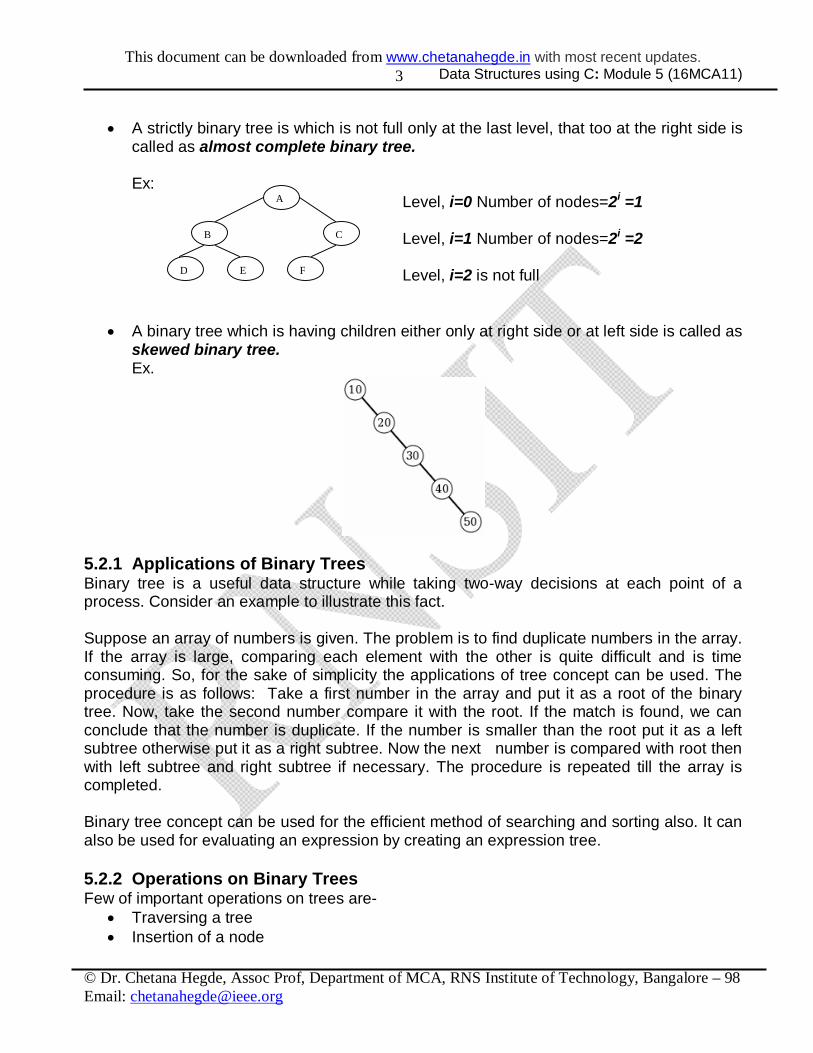
A strictly binary tree is which is not full only at the last level, that too at the right side is called as almost complete binary tree.

Ex:

Level, i=0 Number of nodes=2i =1 Level, i=1 Number of nodes=2i =2 Level, i=2 is not full

A binary tree which is having children either only at right side or at left side is called as skewed binary tree. Ex.

5.2.1 Applications of Binary Trees Binary tree is a useful data structure while taking two-way decisions at each point of a process. Consider an example to illustrate this fact. Suppose an array of numbers is given. The problem is to find duplicate numbers in the array. If the array is large, comparing each element with the other is quite difficult and is time consuming. So, for the sake of simplicity the applications of tree concept can be used. The procedure is as follows: Take a first number in the array and put it as a root of the binary tree. Now, take the second number compare it with the root. If the match is found, we can conclude that the number is duplicate. If the number is smaller than the root put it as a left subtree otherwise put it as a right subtree. Now the next number is compared with root then with left subtree and right subtree if necessary. The procedure is repeated till the array is completed. Binary tree concept can be used for the efficient method of searching and sorting also. It can also be used for evaluating an expression by creating an expression tree. 5.2.2 Operations on Binary Trees Few of important operations on trees are-

Traversing a tree Insertion of a node

A

B C

F D E





4

Deletion of a node Searching for a node

5.2.3 Traversing a Tree Traversal of a tree is a method of visiting each node of a tree exactly once in a systematic way. There are three different methods for tree traversal, viz.

i) Pre-order traversal ii) In-order traversal iii) Post-order traversal

The rules for these traversals are as below- Pre-order traversal:

i) Visit the root. ii) Traverse left subtree using pre-order traversal method. iii) Traverse right subtree using pre-order traversal method.

In-order traversal:

i) Traverse left subtree using in-order traversal method. ii) Visit the root. iii) Traverse right subtree using in-order traversal method.

Post-order traversal:

i) Traverse left subtree using post-order traversal method. ii) Traverse right subtree using pos-order traversal method. iii) Visit the root.

Example: Pre-order: ABDECFG 15, 25, 31, 42, 92, 13, 34, 61 In-order: DBEACGF 31, 42, 25, 92, 15, 34, 13, 61 Post-order: DEBGFCA 42, 31, 92, 25, 34, 61, 13, 15

15

25 13

34 61 31 92

42

A

B C

F

G

D E





5

5.2.4 Representation of Binary Trees For programmatic implementation, tree can be represented in two ways.

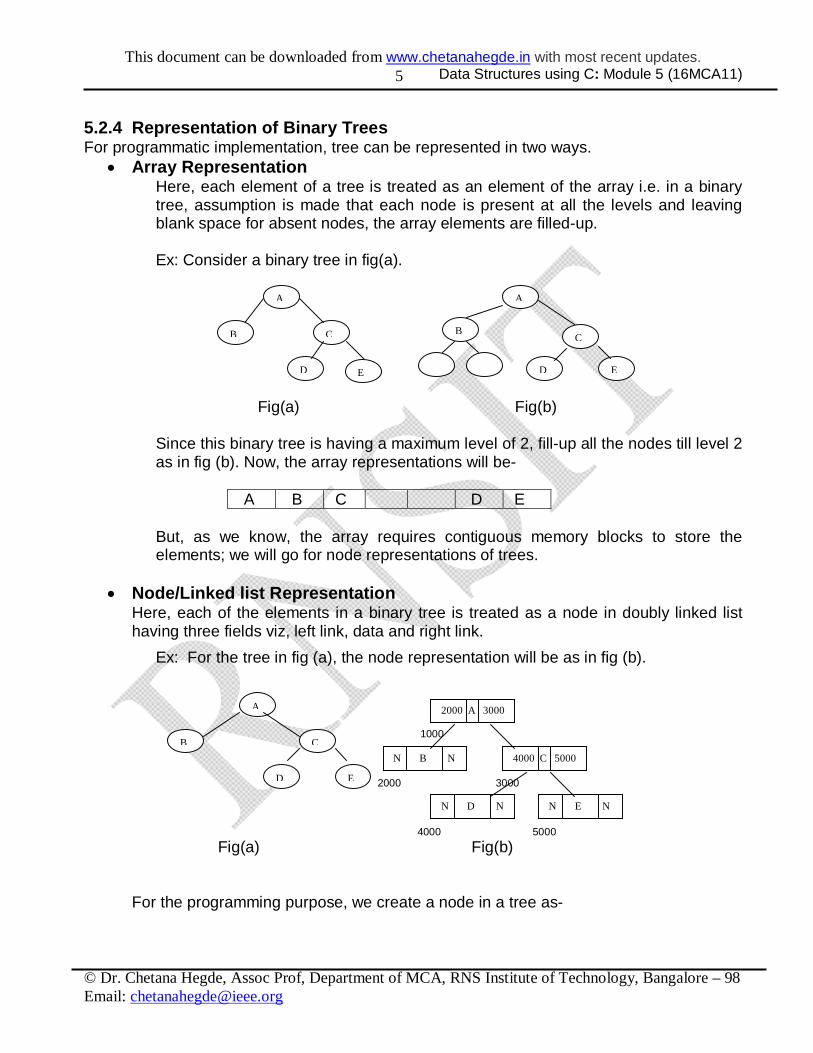
Array Representation Here, each element of a tree is treated as an element of the array i.e. in a binary tree, assumption is made that each node is present at all the levels and leaving blank space for absent nodes, the array elements are filled-up. Ex: Consider a binary tree in fig(a). Fig(a) Fig(b) Since this binary tree is having a maximum level of 2, fill-up all the nodes till level 2 as in fig (b). Now, the array representations will be-

A B C D E But, as we know, the array requires contiguous memory blocks to store the elements; we will go for node representations of trees.

Node/Linked list Representation Here, each of the elements in a binary tree is treated as a node in doubly linked list having three fields viz, left link, data and right link.

Ex: For the tree in fig (a), the node representation will be as in fig (b). 1000 2000 3000 4000 5000 Fig(a) Fig(b)

For the programming purpose, we create a node in a tree as-

A

B C

D E

A

B C

D E

A

B C

D E

2000 A 3000

N B N 4000 C 5000

N D N N E N





6

struct node { struct node *llink; int data; struct node *rlink; }; typedef struct node * NODE;

5.3 BINARY SEARCH TREES Binary search tree is a binary tree in which for each node, the elements in left subtree are less than it and the elements in right subtree are greater than or equal to it. Every node of binary search tree must satisfy this condition. Ex: To insert a new node into BST, it is compared with root. If it is less than the root, traverse towards left subtree. If it is greater than or equal to root, traverse towards right subtree and insertion is made appropriately. Care to be taken such that after insertion also, the tree remains BST. Similary, for deletion of a node also, such precaution is to be taken. Note that in-order traversal of a BST will give the sorted list in ascending order. So, binary tree sort is nothing but a creation of BST and then its in-order traversal. Program: Implementation (creation) of Binary Search Trees and Traversal Techniques #include<stdio.h> #include<conio.h> struct node { struct node *llink; struct node *rlink; int data; }; typedef struct node *NODE; NODE getnode() //Function to get memory from heap { NODE x;

150

100 180

200 50 110

120 85





7

x = (NODE) malloc (sizeof (struct node)); if (x == NULL) { printf("No memory space\n"); exit(0); } return x; } NODE insert (int item, NODE root) //Function to create BST by inserting elements { NODE temp,prev,cur; temp = getnode(); temp->data = item; temp->rlink = NULL; temp->llink = NULL; if(root == NULL) return temp; prev = NULL; cur = root; while (cur != NULL) { prev = cur; cur = (item < cur->data) ? cur->llink : cur->rlink; } if (item < prev->data) prev->llink = temp; else prev->rlink = temp; return root; } void preorder(NODE root) //Function to traverse tree in pre-order { if(root != NULL) { printf("%d\t",root->data); preorder(root->llink);





8

preorder(root->rlink); } } void inorder(NODE root) //Function to traverse tree in in-order { if(root != NULL) { inorder(root->llink); printf("%d\t",root->data); inorder(root->rlink); } } void postorder(NODE root) //Function to traverse tree in post-order { if(root != NULL) { postorder(root->llink); postorder(root->rlink); printf("%d\t",root->data); } } void main() { NODE root = NULL; int opt,item; for(; ;) { printf("\nCreating a Binary Tree and Traversing the tree\n"); printf("Enter your option\n"); printf("1:Insert an element to tree\n"); printf("2:Pre-Order Traversal\n"); printf("3:In-Order Traversal\n"); printf("4:Post-Order Traversal\n"); printf("5:Exit\n"); scanf("%d",&opt); switch(opt) { case 1: printf("Enter the element to be inserted \n"); scanf("%d",&item); root = insert(item,root); break;





9

case 2: printf("PREORDER TRAVERSAL\n"); preorder(root); break; case 3: printf("INORDER TRAVERSAL\n"); inorder(root); break; case 4: printf("POSTORDER TRAVERSAL\n"); postorder(root); break; case 5: default: exit(0); } } } Following is a function for deleting a node from BST. This function can be included in the above program, if you want delete option. /* Function to delete a node whose data field is given*/ NODE deletenode(int key, NODE root) { NODE cur, parent, suc, q; if(root= =NULL) { printf(“empty tree”); return root; } parent=NULL; cur=root; while(cur!=NULL && key!=cur->data) { parent=cur; cur=(item<cur->data)? cur->llink : cur->rlink; } if(cur= =NULL) { printf(“key not found”); return root; } if(cur->llink= =NULL)





10

q= cur ->rlink; else if(cur->rlink= =NULL) q=cur->llink; else { suc=cur->rlink; while(suc->llink!=NULL) suc=suc->llink;

suc->llink=cur->llink; q=cur->rlink; } if(parent= =NULL) return q; if(cur= =parent->llink) parent->llink=q; else parent->rlink=q; free(cur); return root; } 5.4 SORTING Sorting is a process of arranging a set of data in some order. Usually, sorting will be either in ascending order or in descending order. Sorting technique can be mainly divided into two categories viz. internal sorting and external sorting. If all the data to be sorted all stored in the main memory, then it is called as internal sorting. If the data are stored in the auxiliary storage i.e. in floppy, tape etc, then the sorting is said to be external sorting. Let us discuss about different internal sorting techniques one by one. 5.4.1 Selection Sort Selection sort is a simplest method of sorting technique. To sort the given list in ascending order, we will compare the first element with all the other elements. If the first element is found to be greater then the compared element, then they are interchanged. Thus at the end of first interaction, the smallest element will be stored in first position, which is its proper position. Then in the second interaction, we will repeat the procedure from second element to last element. The algorithm is continued till we get sorted list. If there are n elements, we require (n-1) iterations, in general. Consider the example----





11

25 12 30 8 7 43 32 First: Iteration 25 12 30 8 7 43 32 12 25 30 8 7 43 32 12 25 30 8 7 43 32 8 25 30 12 7 43 32 7 25 30 12 8 43 32 7 25 30 12 8 43 32 25 30 12 8 43 32 Second Iteration 25 30 12 8 43 32 25 30 12 8 43 32 12 30 25 8 43 32 8 30 25 12 43 32

8 30 25 12 43 32 30 25 12 43 32

Third Iteration 30 25 12 43 32 25 30 12 43 32 12 30 25 43 32 12 30 25 43 32 30 25 43 32

7

7

7

7

7

7

7 8

7 8

7 8

7 8

7 8

7 8 12





12

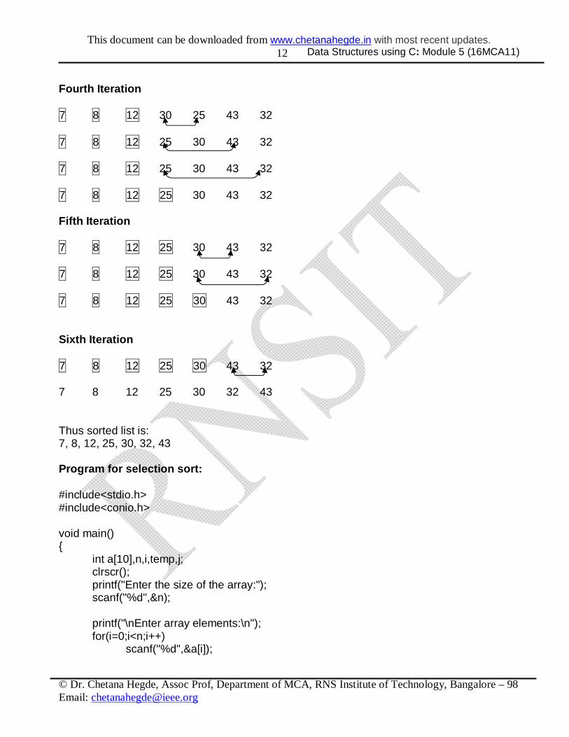
Fourth Iteration 7 8 12 30 25 43 32 7 8 12 25 30 43 32 7 8 12 25 30 43 32 7 8 12 25 30 43 32 Fifth Iteration 7 8 12 25 30 43 32 7 8 12 25 30 43 32 7 8 12 25 30 43 32 Sixth Iteration 7 8 12 25 30 43 32 7 8 12 25 30 32 43 Thus sorted list is: 7, 8, 12, 25, 30, 32, 43 Program for selection sort: #include<stdio.h> #include<conio.h> void main() { int a[10],n,i,temp,j; clrscr(); printf("Enter the size of the array:"); scanf("%d",&n); printf("\nEnter array elements:\n"); for(i=0;i<n;i++) scanf("%d",&a[i]);





13

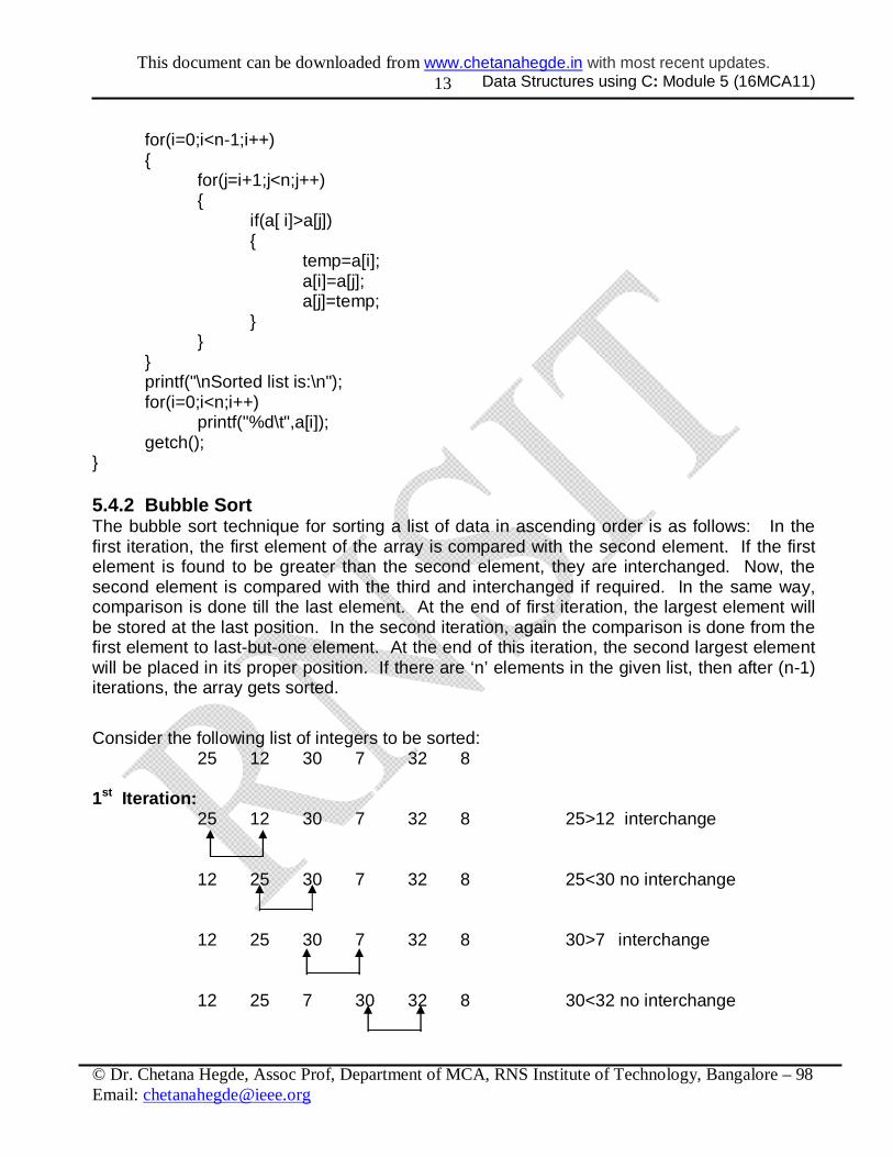
for(i=0;i<n-1;i++) { for(j=i+1;j<n;j++) { if(a[ i]>a[j]) { temp=a[i]; a[i]=a[j]; a[j]=temp; } } } printf("\nSorted list is:\n"); for(i=0;i<n;i++) printf("%d\t",a[i]); getch(); } 5.4.2 Bubble Sort The bubble sort technique for sorting a list of data in ascending order is as follows: In the first iteration, the first element of the array is compared with the second element. If the first element is found to be greater than the second element, they are interchanged. Now, the second element is compared with the third and interchanged if required. In the same way, comparison is done till the last element. At the end of first iteration, the largest element will be stored at the last position. In the second iteration, again the comparison is done from the first element to last-but-one element. At the end of this iteration, the second largest element will be placed in its proper position. If there are ‘n’ elements in the given list, then after (n-1) iterations, the array gets sorted.

Consider the following list of integers to be sorted: 25 12 30 7 32 8 1st Iteration: 25 12 30 7 32 8 25>12 interchange 12 25 30 7 32 8 25<30 no interchange 12 25 30 7 32 8 30>7 interchange 12 25 7 30 32 8 30<32 no interchange





14

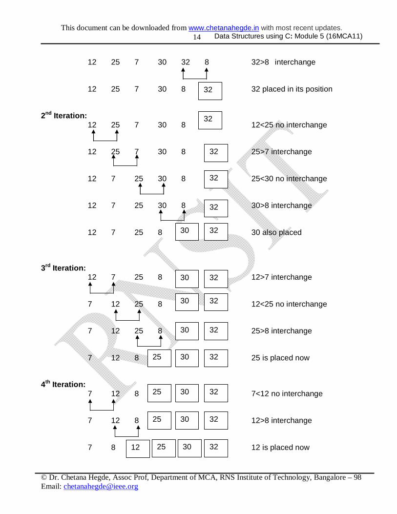
12 25 7 30 32 8 32>8 interchange 12 25 7 30 8 32 placed in its position 2nd Iteration: 12 25 7 30 8 12<25 no interchange 12 25 7 30 8 25>7 interchange

12 7 25 30 8 25<30 no interchange 12 7 25 30 8 30>8 interchange 12 7 25 8 30 also placed 3rd Iteration: 12 7 25 8 12>7 interchange 7 12 25 8 12<25 no interchange 7 12 25 8 25>8 interchange 7 12 8 25 is placed now 4th Iteration: 7 12 8 7<12 no interchange 7 12 8 12>8 interchange 7 8 12 is placed now

32

32

32

32

32

32 30

32 30

32 30

32 30

32 30 25

32 30 25

32 30 25

32 30 25 12





15

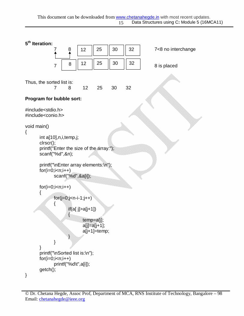
5th Iteration: 7 8 7<8 no interchange 7 8 is placed Thus, the sorted list is: 7 8 12 25 30 32 Program for bubble sort: #include<stdio.h> #include<conio.h> void main() { int a[10],n,i,temp,j; clrscr(); printf("Enter the size of the array:"); scanf("%d",&n); printf("\nEnter array elements:\n"); for(i=0;i<n;i++) scanf("%d",&a[i]); for(i=0;i<n;i++) { for(j=0;j<n-i-1;j++) { if(a[ j]>a[j+1]) { temp=a[j]; a[j]=a[j+1]; a[j+1]=temp; } } } printf("\nSorted list is:\n"); for(i=0;i<n;i++) printf("%d\t",a[i]); getch(); }

32 30 25 12

32 30 25 12 8





16

5.4.3 Insertion Sort This sorting technique involves inserting a particular element in proper position. In the first iteration, the second element is compared with the first. In second iteration, the third element is compared with second and then the first. Thus in every iteration, the element is compared with all the elements before it. If the element is found to be greater than any of its previous elements, then it is inserted at that position and all other elements are moved to one position towards right, to create the space for inserting element. The procedure is repeated till we get the sorted list. Consider an example 25 12 30 8 7 43 32 I iteration 25 12 30 8 7 43 32 (12<25, so insert 12 at first position) 12 25 30 8 7 43 32 II iteration 12 25 30 8 7 43 32 (30>25, so don’t compare 30 with 12) 12 25 30 8 7 43 32 III iteration 12 25 30 8 7 43 32 (8<30,25,12 so insert 8 at 1st position) IV iteration 8 12 25 30 7 43 32 (7<30,25,12,8. So insert 7 at 1st pos) V iteration 7 8 12 25 30 43 32 (43>30. So, don’t compare 43 with other) VI iteration 7 8 12 25 30 43 32 (32<43 but 32>30. So, insert in-between)





17

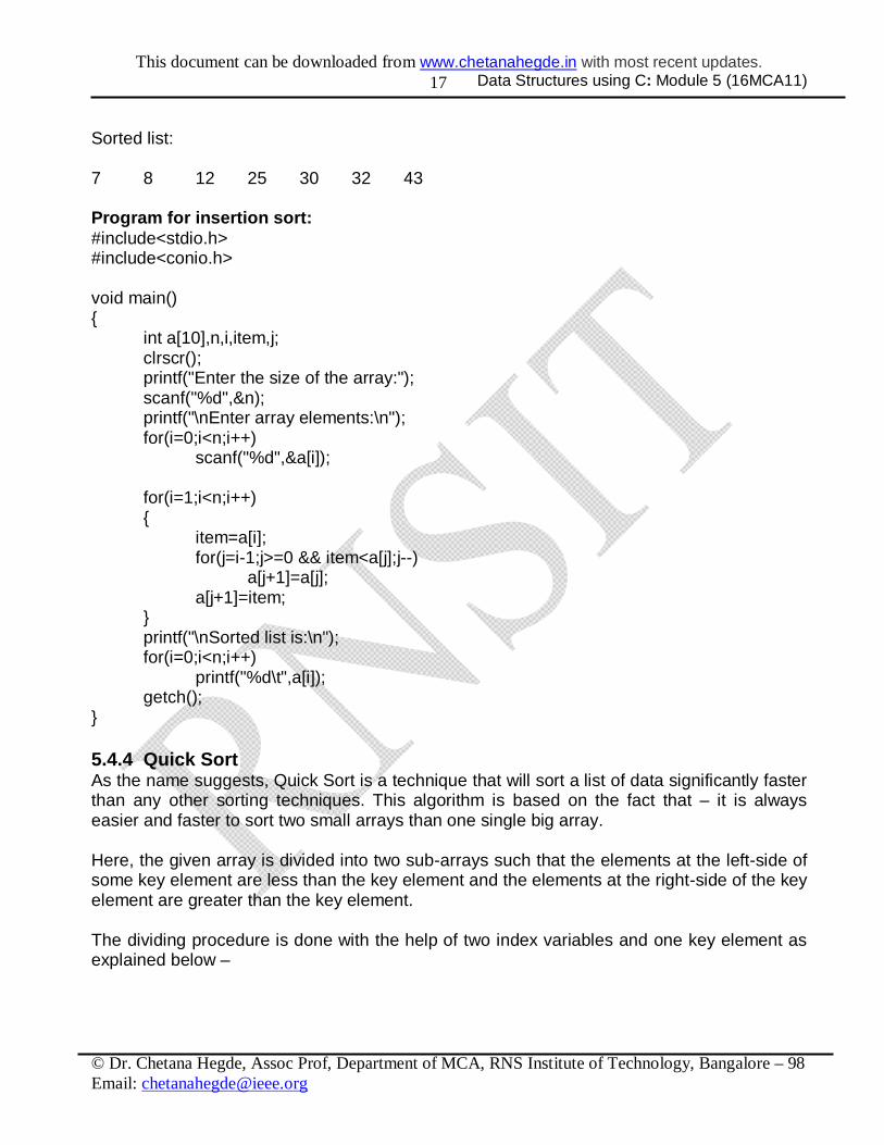
Sorted list: 7 8 12 25 30 32 43 Program for insertion sort: #include<stdio.h> #include<conio.h> void main() { int a[10],n,i,item,j; clrscr(); printf("Enter the size of the array:"); scanf("%d",&n); printf("\nEnter array elements:\n"); for(i=0;i<n;i++) scanf("%d",&a[i]); for(i=1;i<n;i++) { item=a[i]; for(j=i-1;j>=0 && item<a[j];j--) a[j+1]=a[j]; a[j+1]=item; } printf("\nSorted list is:\n"); for(i=0;i<n;i++) printf("%d\t",a[i]); getch(); } 5.4.4 Quick Sort As the name suggests, Quick Sort is a technique that will sort a list of data significantly faster than any other sorting techniques. This algorithm is based on the fact that – it is always easier and faster to sort two small arrays than one single big array. Here, the given array is divided into two sub-arrays such that the elements at the left-side of some key element are less than the key element and the elements at the right-side of the key element are greater than the key element.

The dividing procedure is done with the help of two index variables and one key element as explained below –





18

i) Usually the first element of the array is treated as key. The position of the second element is taken as the first index variable left and the position of the last element will be the index variable right.

ii) Now the index variable left is incremented by one till the value stored at the position left is greater than the key.

iii) Similarly right is decremented by one till the value stored at the position right is smaller than the key.

iv) Now, these two elements are interchanged. Again from the current position, left and right are incremented and decremented respectively and exchanges are made appropriately, if required.

v) This process is continued till the index variables crossover. Now, exchange key with the element at the position right.

vi) Now, the whole array is divided into two parts such that one part is containing the elements less than the key element and the other part is containing the elements greater than the key. And, the position of key is fixed now.

vii) The above procedure (from step i to step vi) is applied on both the sub-arrays. After some iteration we will end-up with sub-arrays containing single element. By that time, the array will be stored.

Let us illustrate this algorithm using an example. Consider an array

a[7] ={25, 12, 30, 8, 7, 43, 32}

Let key =25 left = 1, the position of 12 right =6, the position of 32 First step: Compare key with a[left] key left right

25 12 30 8 7 43 32

Now, key > a[left] (i.e. 25 > 12) is true. So increment left. So, now left will be at the element 30.

Second step: Compare key with a[left]

key left right 25 12 30 8 7 43 32

Now, key > a[left] (i.e. 25 > 30) is false. So stop incrementing left.

Third step: Compare key with a[right].

key left right 25 12 30 8 7 43 32

Now, key < a[right] (i.e. 25 < 32) is true.





19

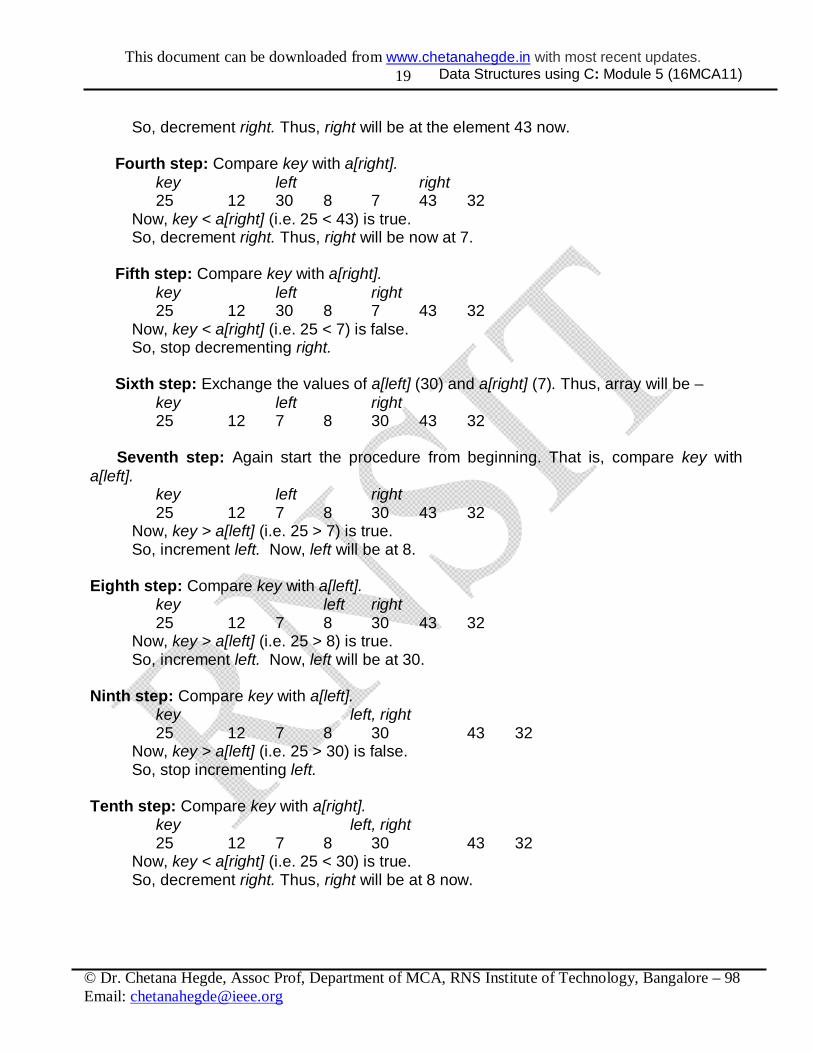
So, decrement right. Thus, right will be at the element 43 now. Fourth step: Compare key with a[right].

key left right 25 12 30 8 7 43 32

Now, key < a[right] (i.e. 25 < 43) is true. So, decrement right. Thus, right will be now at 7. Fifth step: Compare key with a[right].

key left right 25 12 30 8 7 43 32

Now, key < a[right] (i.e. 25 < 7) is false. So, stop decrementing right. Sixth step: Exchange the values of a[left] (30) and a[right] (7). Thus, array will be –

key left right 25 12 7 8 30 43 32

Seventh step: Again start the procedure from beginning. That is, compare key with a[left].

key left right 25 12 7 8 30 43 32

Now, key > a[left] (i.e. 25 > 7) is true. So, increment left. Now, left will be at 8. Eighth step: Compare key with a[left].

key left right 25 12 7 8 30 43 32

Now, key > a[left] (i.e. 25 > 8) is true. So, increment left. Now, left will be at 30. Ninth step: Compare key with a[left].

key left, right 25 12 7 8 30 43 32

Now, key > a[left] (i.e. 25 > 30) is false. So, stop incrementing left. Tenth step: Compare key with a[right].

key left, right 25 12 7 8 30 43 32

Now, key < a[right] (i.e. 25 < 30) is true. So, decrement right. Thus, right will be at 8 now.





20

Eleventh step: The array looks like – key right left 25 12 7 8 30 43 32

As the index variables left and right cross-over, exchange key (25) with a[right] (8). The array would be – 8 12 7 25 30 43 32 Thus, all the elements at the left-side of key(i.e. 25) are less than key and all the elements at the right-side of key are greater than key. Hence, we have got two sub-arrays as – {8, 12, 7} 25 {30, 43, 32} Now, the position of 25 will not get changed. But, we have to sort two sub-arrays separately, by referring the above explained steps.

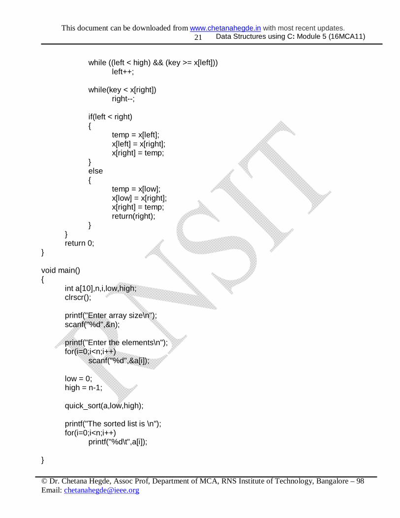
Proceeding like this, we will get the sorted list. Program for quick sort: #include<stdio.h> #include<conio.h> quick_sort(int x[], int low, int high) //Function to apply quick sort technique { int pos; if (low < high) { pos = partition(x,low,high); quick_sort(x,low,pos-1); quick_sort(x,pos+1,high); } return; } int partition(int x[], int low, int high) //Function for partitioning the array { int key, temp, true = 1; int left, right; key = x[low]; left = low +1; right = high; while(true) {





21

while ((left < high) && (key >= x[left])) left++; while(key < x[right]) right--;

if(left < right) { temp = x[left]; x[left] = x[right]; x[right] = temp; } else { temp = x[low]; x[low] = x[right]; x[right] = temp; return(right); } } return 0; } void main() { int a[10],n,i,low,high; clrscr(); printf("Enter array size\n"); scanf("%d",&n); printf("Enter the elements\n"); for(i=0;i<n;i++) scanf("%d",&a[i]); low = 0; high = n-1; quick_sort(a,low,high); printf("The sorted list is \n"); for(i=0;i<n;i++) printf("%d\t",a[i]); }





22

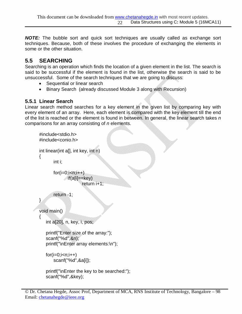
NOTE: The bubble sort and quick sort techniques are usually called as exchange sort techniques. Because, both of these involves the procedure of exchanging the elements in some or the other situation. 5.5 SEARCHING Searching is an operation which finds the location of a given element in the list. The search is said to be successful if the element is found in the list, otherwise the search is said to be unsuccessful. Some of the search techniques that we are going to discuss:

Sequential or linear search Binary Search (already discussed Module 3 along with Recursion)

5.5.1 Linear Search Linear search method searches for a key element in the given list by comparing key with every element of an array. Here, each element is compared with the key element till the end of the list is reached or the element is found in between. In general, the linear search takes n comparisons for an array consisting of n elements.

#include<stdio.h> #include<conio.h> int linear(int a[], int key, int n) { int i; for(i=0;i<n;i++) if(a[i]==key) return i+1; return -1; } void main() { int a[20], n, key, i, pos; printf("Enter size of the array:"); scanf("%d",&n); printf("\nEnter array elements:\n"); for(i=0;i<n;i++) scanf("%d",&a[i]); printf("\nEnter the key to be searched:"); scanf("%d",&key);





23

pos=linear(a, key, n); if(pos==-1) printf("\nUnsuccessful search!!"); else printf("\nKey found at position %d",pos); }

5.6 HASHING Hashing is a way of representing dictionaries. Dictionary is an abstract data type with a set of operations searching, insertion and deletion defined on its elements. The elements of dictionary can be numeric or characters or most of the times, records. Usually, a record consists of several fields; each may be of different data types. For example, student record may contain student id, name, gender, marks etc. Every record is usually identified by some key. Here we will consider the implementation of a dictionary of n records with keys k1, k2 …kn. Hashing is based on the idea of distributing keys among a one-dimensional array

H[0…m-1], called hash table.

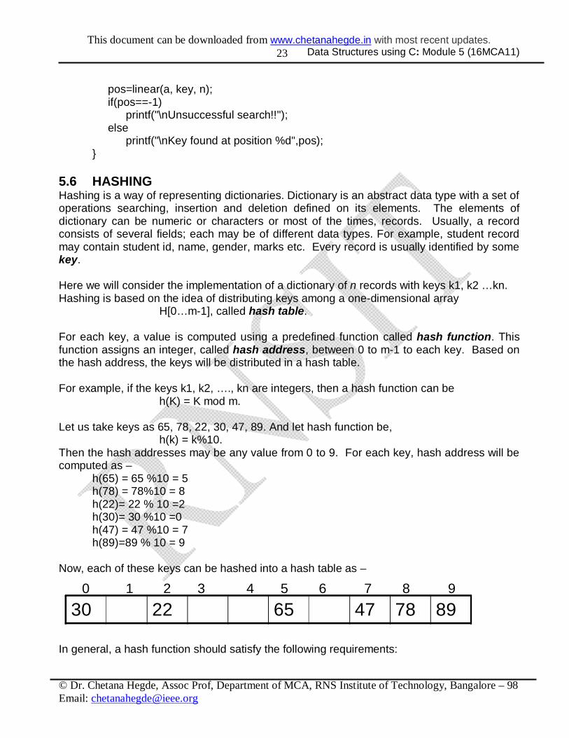
For each key, a value is computed using a predefined function called hash function. This function assigns an integer, called hash address, between 0 to m-1 to each key. Based on the hash address, the keys will be distributed in a hash table. For example, if the keys k1, k2, …., kn are integers, then a hash function can be h(K) = K mod m. Let us take keys as 65, 78, 22, 30, 47, 89. And let hash function be,

h(k) = k%10. Then the hash addresses may be any value from 0 to 9. For each key, hash address will be computed as – h(65) = 65 %10 = 5 h(78) = 78%10 = 8 h(22)= 22 % 10 =2 h(30)= 30 %10 =0 h(47) = 47 %10 = 7 h(89)=89 % 10 = 9 Now, each of these keys can be hashed into a hash table as –

30 22 65 47 78 890 1 2 3 4 5 6 7 8 9

In general, a hash function should satisfy the following requirements:





24

A hash function needs to distribute keys among the cells of hash table as evenly as possible.

A hash function has to be easy to compute. 5.6.1 Hash Collisions Let us have n keys and the hash table is of size m such that m<n. As each key will have an address with any value between 0 to m-1, it is obvious that more than one key will have same hash address. That is, two or more keys need to be hashed into the same cell of hash table. This situation is called as hash collision. In the worst case, all the keys may be hashed into same cell of hash table. But, we can avoid this by choosing proper size of hash table and hash function. Anyway, every hashing scheme must have a mechanism for resolving hash collision. There are two methods for hash collision resolution, viz.

Open hashing or Separate Chaining Closed hashing or Open Addressing

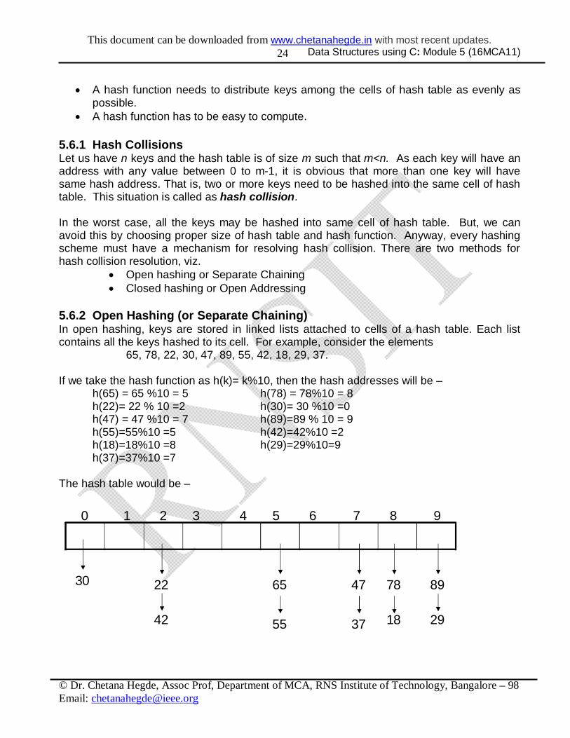
5.6.2 Open Hashing (or Separate Chaining) In open hashing, keys are stored in linked lists attached to cells of a hash table. Each list contains all the keys hashed to its cell. For example, consider the elements 65, 78, 22, 30, 47, 89, 55, 42, 18, 29, 37. If we take the hash function as h(k)= k%10, then the hash addresses will be –

h(65) = 65 %10 = 5 h(78) = 78%10 = 8 h(22)= 22 % 10 =2 h(30)= 30 %10 =0 h(47) = 47 %10 = 7 h(89)=89 % 10 = 9 h(55)=55%10 =5 h(42)=42%10 =2 h(18)=18%10 =8 h(29)=29%10=9 h(37)=37%10 =7

The hash table would be –

0 1 2 3 4 5 6 7 8 9

65 7830 22 47

55 1842

89

37 29





25

Operations on Hashing: Searching: Now, if we want to search for the key element in a hash table, we need to

find the hash address of that key using same hash function. Using the obtained hash address, we need to search the linked list by tracing it, till either the key is found or list gets exhausted.

Insertion: Insertion of new element to hash table is also done in similar manner. Hash key is obtained for new element and is inserted at the end of the list for that particular cell.

Deletion: Deletion of element is done by searching that element and then deleting it from a linked list.

5.6.3 Closed Hashing (or Open Addressing) In this technique, all keys are stored in the hash table itself without using linked lists. Different methods can be used to resolve hash collisions. The simplest technique is linear probing. This method suggests to check the next cell from where the collision occurs. If that cell is empty, the key is hashed there. Otherwise, we will continue checking for the empty cell in a circular manner. Thus, in this technique, the hash table size must be at least as large as the total number of keys. That is, if we have n elements to be hashed, then the size of hash table should be greater or equal to n. Example: Consider the elements 65, 78, 18, 22, 30, 89, 37, 55, 42 Let us take the hash function as h(k)= k%10, then the hash addresses will be – h(65) = 65 %10 = 5 h(78) = 78%10 = 8

h(18)=18%10 =8 h(22)= 22 % 10 =2 h(30)= 30 %10 =0 h(89)=89 % 10 = 9 h(37)=37%10 =7 h(55)=55%10 =5 h(42)=42%10 =2

Since there are 9 elements in the list, our hash table should at least be of size 9. Here we are taking the size as 10. Now, hashing is done as below –

NOTE: When we resolve collisions through closed hashing, the hash table may end-up without proper order of storage. Hence, searching may become like a linear search and hence it is not efficient.

30 89 22 42 65 55 37 78 18 0 1 2 3 4 5 6 7 8 9



TREES, SORTING AND SEARCHING - Chetana Hegde · TREES, SORTING AND SEARCHING 5.1 INTRODUCTION TO TREES The data structures that we studied till now such as stack, queue, linked list

Documents