Statistics and Computing 14: 143–166, 2004 C 2004 Kluwer Academic Publishers. Manufactured in The Netherlands. Tree consistency and bounds on the performance of the max-product algorithm and its generalizations MARTIN WAINWRIGHT ∗ , TOMMI JAAKKOLA † and ALAN WILLSKY † ∗ Electrical Engineering & Computer Science, UC Berkeley, Berkeley, CA [email protected] † Electrical Engineering & Computer Science, MIT, Cambridge, MA [email protected]; [email protected] Received December 2002 and accepted November 2003 Finding the maximum a posteriori (MAP) assignment of a discrete-state distribution specified by a graphical model requires solving an integer program. The max-product algorithm, also known as the max-plus or min-sum algorithm, is an iterative method for (approximately) solving such a problem on graphs with cycles. We provide a novel perspective on the algorithm, which is based on the idea of reparameterizing the distribution in terms of so-called pseudo-max-marginals on nodes and edges of the graph. This viewpoint provides conceptual insight into the max-product algorithm in application to graphs with cycles. First, we prove the existence of max-product fixed points for positive distributions on arbitrary graphs. Next, we show that the approximate max-marginals computed by max-product are guaranteed to be consistent, in a suitable sense to be defined, over every tree of the graph. We then turn to characterizing the nature of the approximation to the MAP assignment computed by max- product. We generalize previous work by showing that for any graph, the max-product assignment satisfies a particular optimality condition with respect to any subgraph containing at most one cycle per connected component. We use this optimality condition to derive upper bounds on the difference between the log probability of the true MAP assignment, and the log probability of a max-product assignment. Finally, we consider extensions of the max-product algorithm that operate over higher- order cliques, and show how our reparameterization analysis extends in a natural manner. Keywords: MAP estimation, integer programming, max-product, min-sum, max-plus, graphical models, max-marginals, inference, iterative decoding, Viterbi algorithm, dynamic programming 1. Introduction Integer programming problems are important in a variety of fields, including artificial intelligence and statistics (e.g., Pearl 1988, Dawid 1992, Cowell et al. 1999), statistical physics (e.g., Barahona 1982), error-correcting coding (e.g., Aji et al. 1998, Gallager 1963), and statistical image processing (e.g., Besag 1986, Geman and Geman 1984). Such problems, which entail optimizing a cost function over some subset of the integers, can in many cases be formulated in terms of graphical models (e.g., Cowell et al. 1999, Jordan 1999). In the formalism of such models, the cost function to be maximized corresponds to a distribution that factorizes as a product of terms over cliques of the graph, and the associated optimization problem is to find the maximum a posteriori (MAP) configuration. The complexity of this MAP estimation problem turns out to depend critically on the structure of the underlying graph. On one hand, for a graph without cycles (i.e., a tree), the MAP configuration can be computed efficiently by algorithms in which nodes convey information to one another by passing messages. Updates of this type are known under various names, including belief revision (Pearl 1988), as well as the max-product or min- sum algorithm (e.g., Aji and McEliece 2000). One way to view max-product updates is as a parallel implementation of standard dynamic programming updates (Bertsekas 1995); in this sense, they represent a generalization of the Viterbi algorithm (Viterbi 1967, Forney 1973) from a chain-structured graph to an arbitrary tree. On such tree-structured graphs, it is well-known that the message-passing updates converge, and yield the correct MAP assignment after a finite number of steps (e.g., Pearl 1988). 0960-3174 C 2004 Kluwer Academic Publishers

Welcome message from author
This document is posted to help you gain knowledge. Please leave a comment to let me know what you think about it! Share it to your friends and learn new things together.
Transcript

Statistics and Computing 14: 143–166, 2004C© 2004 Kluwer Academic Publishers. Manufactured in The Netherlands.
Tree consistency and bounds on theperformance of the max-product algorithmand its generalizations
MARTIN WAINWRIGHT∗, TOMMI JAAKKOLA† and ALAN WILLSKY†
∗Electrical Engineering & Computer Science, UC Berkeley, Berkeley, [email protected]†Electrical Engineering & Computer Science, MIT, Cambridge, [email protected]; [email protected]
Received December 2002 and accepted November 2003
Finding the maximum a posteriori (MAP) assignment of a discrete-state distribution specified by agraphical model requires solving an integer program. The max-product algorithm, also known as themax-plus or min-sum algorithm, is an iterative method for (approximately) solving such a problemon graphs with cycles. We provide a novel perspective on the algorithm, which is based on the idea ofreparameterizing the distribution in terms of so-called pseudo-max-marginals on nodes and edges ofthe graph. This viewpoint provides conceptual insight into the max-product algorithm in application tographs with cycles. First, we prove the existence of max-product fixed points for positive distributionson arbitrary graphs. Next, we show that the approximate max-marginals computed by max-productare guaranteed to be consistent, in a suitable sense to be defined, over every tree of the graph. Wethen turn to characterizing the nature of the approximation to the MAP assignment computed by max-product. We generalize previous work by showing that for any graph, the max-product assignmentsatisfies a particular optimality condition with respect to any subgraph containing at most one cycleper connected component. We use this optimality condition to derive upper bounds on the differencebetween the log probability of the true MAP assignment, and the log probability of a max-productassignment. Finally, we consider extensions of the max-product algorithm that operate over higher-order cliques, and show how our reparameterization analysis extends in a natural manner.
Keywords: MAP estimation, integer programming, max-product, min-sum, max-plus, graphicalmodels, max-marginals, inference, iterative decoding, Viterbi algorithm, dynamic programming
1. Introduction
Integer programming problems are important in a variety offields, including artificial intelligence and statistics (e.g., Pearl1988, Dawid 1992, Cowell et al. 1999), statistical physics (e.g.,Barahona 1982), error-correcting coding (e.g., Aji et al. 1998,Gallager 1963), and statistical image processing (e.g., Besag1986, Geman and Geman 1984). Such problems, which entailoptimizing a cost function over some subset of the integers,can in many cases be formulated in terms of graphical models(e.g., Cowell et al. 1999, Jordan 1999). In the formalism of suchmodels, the cost function to be maximized corresponds to adistribution that factorizes as a product of terms over cliques ofthe graph, and the associated optimization problem is to find themaximum a posteriori (MAP) configuration.
The complexity of this MAP estimation problem turns outto depend critically on the structure of the underlying graph.On one hand, for a graph without cycles (i.e., a tree), the MAPconfiguration can be computed efficiently by algorithms in whichnodes convey information to one another by passing messages.Updates of this type are known under various names, includingbelief revision (Pearl 1988), as well as the max-product or min-sum algorithm (e.g., Aji and McEliece 2000). One way to viewmax-product updates is as a parallel implementation of standarddynamic programming updates (Bertsekas 1995); in this sense,they represent a generalization of the Viterbi algorithm (Viterbi1967, Forney 1973) from a chain-structured graph to an arbitrarytree. On such tree-structured graphs, it is well-known that themessage-passing updates converge, and yield the correct MAPassignment after a finite number of steps (e.g., Pearl 1988).
0960-3174 C© 2004 Kluwer Academic Publishers

144 Wainwright, Jaakkola and Willsky
Dawid (1992) described how to compute the MAP configu-ration for more general graphs by first converting to a junctiontree representation, and then performing dynamic programmingin the junction tree. Nilsson (1998) analyzed this algorithm inmore detail, and showed how a partitioning scheme can be usedto compute the M most probable configurations. The complex-ity of such exact methods scales exponentially in the size of thelargest clique in the junction tree, a quantity closely related tothe graph treewidth (see Bodlaender 1993). Unfortunately, formany graphs with cycles, this treewidth becomes so large thatthe junction tree approach is no longer feasible. This intractabil-ity motivates the development and use of approximate methodsfor computing MAP assignments on graphs with cycles.
The focus of this paper is a “loopy” version of the max-product algorithm, in which the usual message-passing updatesare applied in parallel to a graph with cycles. This use of themax-product algorithm for computing approximate MAP as-signments on graphs with cycles has been the focus of con-siderable research in recent years (e.g., Aji et al. 1998, Horn1999, Forney et al. 2001a, b, Frey, Koetter and Vardy 2001,Weiss 2000, Freeman and Weiss 2001). As a consequence ofthe presence of cycles, the max-product updates are no longerguaranteed to converge. Nonetheless, the loopy max-product al-gorithm has been used with good results in various applications,including decoding of graphical codes (e.g., Benedetto et al.1996, Aji et al. 1998, Wiberg 1996) as well as computer vision(e.g., Freeman and Pasztor 1999). Most previous analysis of themax-product algorithm for graphs with cycles is based on anidea that dates back to the work of Gallager (1963)—namely,that of studying the computation tree associated with the paral-lel message-passing updates. Given some node specified as theroot, the corresponding computation tree (at iteration n) repre-sents the set of all possible paths (of length n) that end at thisroot node; any such path corresponds to the propagation of in-formation in a message from some initial node to the root. Moredetails on such computation trees can be found in (e.g., Gallager1963, Wiberg 1966, Frey et al. 2001, Weiss 2000, Freeman andWeiss 2001). A number of researchers have studied the max-product algorithm in application to a single cycle (e.g., Weiss2000, Horn 1999, Aji et al. 1998, Frey, Koetter and Vardy 2001;Forney et al. 2001b), for which the computation tree is especiallysimple—namely, a chain-structured graph. For a single cycle, themessage passing updates converge to either a stable fixed point,or a periodic oscillation. When it converges to stable fixed point,the max-product assignment is guaranteed to be exact, as long asa certain uniqueness condition (to be specified) holds. Freemanand Weiss (2001) analyzed the max-product assignment for posi-tive compatibility functions on arbitrary graphs, and showed thatthe cost of the max-product assignment cannot be improved bychanging any subset of the variables that form no more than asingle cycle in the underlying graph. In the context of graphsdefined by codes, Frey and Koetter (2000) showed that if max-product messages are suitably attenuated as they are passed upthe computation tree, then the algorithm (if it converges) com-putes the MAP assignment. For the special case of cycle codes,1
Wiberg (1996) gave sufficient conditions for max-product to failto converge to the transmitted codeword; see also Horn (1999)for related results on cycle codes. For the ferromagnetic Isingmodel,2 Fridman (2002) showed how to assess the correctness ofthe max-product assignment in an a priori manner (i.e., beforeeven running the algorithm).
The analysis of this paper, in contrast to previous work usingcomputation trees, is based on a different perspective. Any distri-bution defined by a graphical model is represented as a productof so-called compatibility functions over cliques of the under-lying graph. Since the factorization is not unique, it is temptingto seek alternative representations that have desirable propertiesfor solving inference problems. In previous work (Wainwright,Jaakkola and Willsky 2003), we have shown that the sum-productor belief propagation algorithm for graphs with cycles can beviewed as seeking a particular reparameterization of the distri-bution. In this paper, we show that the conceptual framework ofreparameterization can be applied fruitfully to the max-productalgorithm on graphs with cycles as well.
More specifically, the complexity of the MAP estimationproblem stems from the specification of the overall distribu-tion as a (normalized) product of compatibility functions on thecliques of the graph. These functions couple together the opti-mization of variables at all the nodes. However, the factoriza-tion of the overall distribution is not unique, which suggests theidea of finding a new factorization—that is, reparameterizingthe distribution—in terms of functions that reduce or removethis coupling. For a distribution on a decomposable graph, avariant of the junction tree theorem (Dawid 1992, Cowell et al.1999) yields a factorization in terms of so-called max-marginalson the maximal cliques and separator sets of the junction tree.As we elucidate in Section 3 for trees, the message-passing ofthe max-product algorithm can be understood as computing thismax-marginal factorization.
At one level, then, solving the MAP estimation problem on adecomposable graph can be viewed as converting from the orig-inal representation into a form that makes extracting the MAPestimate computationally simple. Indeed, if each single-nodemax-marginal has a unique maximum, then the overall MAP esti-mate can be computed by performing decoupled maximizationsof the max-marginals at each node. As we discuss in Section 3,the violation of this assumption is only a minor issue for tree-structured distributions. In fact, since the max-product algorithmalso computes pairwise max-marginals, dynamic programmingmethods can be applied to the tree in order to compute one ofthe MAP estimates. (See also Dawid (1992) for description of asimilar sampling procedure for junction trees.) However, as weillustrate by example in Section 4, when the uniqueness assump-tion is violated for a graph with cycles, the max-marginals areat best problematic, and at worst very misleading. Thus, a minorcontribution of our paper is to identify the importance of theuniqueness assumption both for our analysis, and for the utilityof max-product in application to graphs with cycles.
The reparameterization perspective motivates the idea of con-sidering a sequence of updates on trees embedded within a graph

Performance of the max-product algorithm and its generalizations 145
with cycles. Each such update consists of reparameterizing thesubset of factors defining the distribution that correspond to(nodes and edges in) the tree, while leaving untouched the re-maining factors. More specifically, the reparameterization forthe tree terms is specified by what we refer to as a set of pseudo-max-marginals. The main results of this paper, which are pre-sented in Section 4, are based on a detailed analysis of such se-quences of reparameterization updates. In this section, we provethat fixed points of such updates are equivalent to those of theusual message-passing updates. This equivalence allows us toanalyze max-product in terms of reparameterization as opposedto the usual message-passing updates. For a graph with cycles,it is not obvious that fixed points of the max-product algorithmnecessarily exist. A number of researchers (e.g., Aji et al. 1998,Weiss 2000) have shown the existence of fixed points for positivecompatibility functions on a single cycle graph. We generalizethis result by proving that max-product fixed points exist forany positive distribution on an arbitrary graph with cycles. Aninteresting implication is that any positive distribution can befactorized in terms of a set of pseudo-max-marginals that areconsistent (in a sense that we make precise) on every spanningtree of the graph. We also show in Section 4 that the uniquenessof the single-node maximizers is critical if the pseudo-max-marginals are to be of any value for MAP estimation. Further-more, under the assumption of uniqueness, we prove that themax-product assignment on a graph G with cycles is guaran-teed to be “optimal” on any subgraph of G containing at mostone cycle, where “optimality” here refers to the inability to ob-tain a better assignment for a modified cost function formed bythe product of terms corresponding to the subgraph. This the-orem generalizes earlier results by Weiss (2000), and Freemanand Weiss (2001) mentioned previously. Using this optimalitytheorem, we then derive a set of computable upper bounds on thedifference between the log probability of the MAP assignment,and the log probability of the max-product assignment on an ar-bitrary graph with cycles, and we illustrate the consequences ofthese bounds. In Section 5 and in analogy to recent generaliza-tions of the sum-product algorithm (e.g., Yedidia, Freeman andWeiss 2001), we consider generalizations of the max-productalgorithm that operate over higher order cliques. An attractivefeature of our reparameterization analysis is that it extends verynaturally to these generalizations.
2. Background
In this section, we first provide some basic background on graphtheory, giving only those concepts necessary for subsequent de-velopments; we refer the reader to the books by Bollobas (1998)and Berge (1976) for further background. We then discuss theformalism of graphical models—in particular, Markov randomfields—as well as the associated MAP estimation problem. Moredetails about graphical models can be found in various sources(e.g., Cowell et al. 1999, Lauritzen 1996, Jordan 1999).
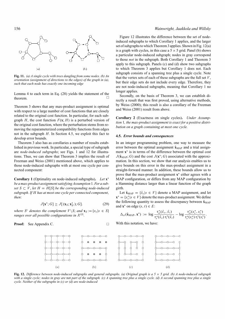
Fig. 1. Illustration of a node-induced subgraph. (a) Original graph G.(b) Subgraph H[S] induced by the subset of nodes S = {1, 2, 3, 5, 6, 8}
2.1. Graph-theoretic basics
An undirected graph G = (V, E) consists of a set of nodes orvertices V = {1, . . . , N } that are joined by a set of edges E .Throughout this paper, we focus on simple graphs, for whichmultiple edges between the same pair of vertices as well as self-loops (i.e., an edge from a node back to itself) are forbidden.For each s ∈ V , let N (s) = {t ∈ V | (s, t) ∈ E} denote the setof neighbors of s. A clique of the graph G is any subset of thevertex set V for which each node is connected to every other.A clique is maximal if it is not properly contained within anyother clique. Note that any single node is itself a clique, but nota maximal clique unless it has no neighbors.
A subgraph H = (V (H ), E(H )) of the graph G is a graphformed by subsets V (H ) and E(H ) of the vertex and edge sets (Vand E respectively). A spanning subgraph is one that includesevery vertex of the graph (i.e., V (H ) = V ). In the sequel, it willbe important to consider node-induced subgraphs. In particular,given a subset S ⊂ V , the corresponding node-induced subgraphH [S] is formed by the vertex set V (S) = S and the edge setE(S) = { (s, t) ∈ E | s, t ∈ S }. Figure 1 provides an illustrationof a node-induced subgraph. A path is a graph P consistingof a set of vertices V (P) = {s0, s1, . . . , sk} and a collection ofdistinct edges E(P) = {(s0, s1), . . . (sk−1, sk)}. We say that P isa path from s0 to sk . A graph is connected if for each pair {s, t}of distinct vertices, there is a path from s to t . A component ofa graph is a maximal connected subgraph.
Graphs without cycles play an important role in our analysis.A tree T is a cycle-free graph consisting of a single connectedcomponent; a spanning tree is an acyclic subgraph whose vertexset is all of V . See Fig. 2 for an illustration of a spanning tree.A leaf node of a tree is a vertex with a single neighbor; any
Fig. 2. (a) Graph G with cycles. (b) Embedded spanning tree thatreaches each vertex of G

146 Wainwright, Jaakkola and Willsky
Fig. 3. Illustration of graph separation. With all paths that pass throughsubset B blocked, the two sets A and C are separated. Thus, B forms avertex cutset for the graph
tree with N ≥ 2 nodes is guaranteed to have at least two leaves(Bollobas 1998).
2.2. Markov random fields and MAP estimation
Given an undirected graph G, we associate with each node sin the vertex set a discrete random variable xs taking values inthe discrete space X = {0, . . . , m − 1}. The full vector x ={ xs | s ∈ V } takes values in the Cartesian product space X N . Ofinterest to us are random vectors x that respect a set of Markovproperties associated with the graph. In particular, let A, B, andC be three disjoint subsets of the vertex set, and suppose that Bseparates A from C (as illustrated in Fig. 3). We then require thatthe collection of random variables in A (i.e., xA = {xs | s ∈ A})is conditionally independent of those in C (i.e., xC ), given thevariables xB . The random vector x is a Markov random field ifit respects all such properties associated with G.
Given a clique C of the graph G, a compatibility function isa mapping ψC : X N → R
+ that depends only on the subvectorxC = {xs | s ∈ C}. The Hammersley-Clifford theorem (e.g.,Bremaud 1991) guarantees that a random vector x with strictlypositive distribution p(x) is a Markov random field (MRF) withrespect to G if and only if the distribution factorizes as a productof compatibility functions over cliques:
p(x) = 1
Z
∏C∈C
ψC(xC). (1)
Here C is the set of all cliques of G, and Z = ∑x
∏C∈C ψC(xC)
is the partition function that normalizes the distribution.As is standard in most treatments of the sum-product or max-
product algorithms (e.g., Pearl 1988, Weiss 2000), the bulk ofthis paper treats pairwise Markov random fields, for which Ghas only singleton and pairwise cliques. In Section 5, we showhow the ordinary max-product algorithm can be extended toaccommodate higher-order cliques, and how our analysis appliesto these generalizations as well. For a pairwise Markov randomfield, the set of cliques is given by V ∪ E , so that we have acompatibility function ψs for each node, and a function ψst foreach edge (s, t) ∈ E . In this case, Eq. (1) assumes the followingsimpler form:
p(x) = 1
Z
∏s∈V
ψs(xs)∏
(s,t)∈E
ψst (xs, xt ). (2)
The effect of including independent noisy observation ys of xs
at each node is to modify the singleton compatibility functions.Since the addition of observations can be modeled by Eq. (2),we suppress any explicit reference to measurements throughoutthis paper.
The problem of maximum a posteriori (MAP) estimation cor-responds to finding a configuration that is most likely under thedistribution p(x) defined in Eq. (1). In more formal terms, anyMAP configuration xMAP is defined by the relation
xMAP = arg maxx∈X N
p(x). (3)
Note that the MAP configuration need not be unique; that is,there may be multiple configurations that attain the maximumin Eq. (3). In this case, we refer to each one as a possible MAPconfiguration.
Equivalently, we can formulate the MAP problem as findingthe configuration x ∈ X N that maximizes the function:
J (x; G ) :=∑s∈V
log ψs(xs) +∑
(s,t)∈E
log ψst (xs, xt ). (4)
Note that any unconstrained integer programming problem inwhich variables interact in a pairwise manner can be expressedin the form of Eq. (4). Examples include the minimum s − tcut and multiway-cut problems in combinatorial optimization(e.g., Grotschel et al. 1993), image segmentation on a grid (e.g.,Geman and Geman 1984), and calculating ground states in theIsing model of statistical physics (e.g., Barahona 1982).
3. MAP estimation on trees
The focus of this section is the problem of MAP estimationfor tree-structured graphs, in which context we introduce max-marginals and the max-product algorithm. This section is, inpart, continued background, but it also provides several impor-tant observations that are critical for our main development inSection 4. In Section 3.1, we review the factorization of any tree-structured distribution in terms of its max-marginals, as guaran-teed by the junction tree theorem (e.g., Cowell et al. 1999, Dawid1992). We also show that the use of the max-marginals for MAPestimation requires some care if the single-node maximizers failto be unique. In Section 3.2, we introduce the max-product al-gorithm in the context of tree-structured distributions, and provethat this algorithm exactly computes the reparameterization ofthe overall distribution in terms of max-marginals. This inter-pretation is key to our analysis in Section 4 of max-producton graphs with cycles, in which case the quantities computedby the max-product algorithm represent only approximations tothe true max-marginals.
3.1. Role of max-marginals
We begin by defining the max-marginals associated with any dis-tribution p(x). For each xs ∈ X , the value of the max-marginalµs(xs) associated with node s ∈ V is given by maximizing p(x)

Performance of the max-product algorithm and its generalizations 147
over the subset of configurations {x′ ∈ X N | x ′s = xs}—viz.:
µs(xs) = κ max{x′ |x ′
s=xs }p(x′). (5)
Here κ denotes a positive but otherwise arbitrary normalizationconstant; for example, it can be chosen so that maxx ′
sµs(x ′
s) = 1.We use this notation throughout the paper, where the value of κ
may differ from node to node, and from line to line.Note that µs(xs) is proportional to the probability of the most
likely configuration x′ with x ′s fixed to the value of xs . In an
analogous fashion, we can define pairwise max-marginals forpairs of nodes (s, t) ∈ E :
µst (xs, xt ) := κ max{x′|(x ′
s ,x′t )=(xs ,xt )}
p(x′). (6)
Again, µst (xs, xt ) is proportional to the probability of the mostlikely configuration x′ ∈ X N subject to the constraint that x ′
s =xs and x ′
t = xt .The original representation of p(x) given in Eq. (2) is in terms
of compatibility functions on the nodes and edges of the graph.One remarkable property of any tree-structured distribution isthat it can also be factorized in terms of its max-marginals:
Theorem 1 (Tree factorization). Any tree-structured distribu-tion p(x) has the following alternative factorization in terms ofits max-marginals:
p(x) ∝∏s∈V
µs(xs)∏
(s,t)∈E
µst (xs, xt )
µs(xs)µt (xt ), (7)
where the max-marginals µ = {µs, µst } are defined in Eqs. (5)and (6) respectively.
Equation (7) is a special case of the more general junction treerepresentation (Cowell et al. 1999, Dawid 1992). In Section 3.2,we provide, as a by-product of our presentation of the max-product algorithm, a constructive proof of the factorization inTheorem 1.
For the time being, suppose that we have computed the com-plete set of max-marginals µ = {µs, µst }. We now consider theproblem of using the max-marginals to obtain an MAP config-uration. If, for each node, the maximum of µs over x ′
s ∈ X isattained at a unique value, then it can be seen that the MAP con-figuration xMAP = {xs | s ∈ V } is unique, with elements givenby x s = arg maxx ′
s∈X µs(x ′s). Note the benefit of converting p(x)
to the alternative max-marginal representation: instead of glob-ally optimizing the distribution in Eq. (2), a local optimizationat each node—i.e., maximizing µs(xs)—suffices to obtain theMAP configuration.
Suppose, on the other hand, that for at least one node s ∈ V ,there exist multiple states xs that attain the maximum of µs . Inthis case, there must be multiple MAP configurations (at leastone for each state xs that achieves the maximum); moreover,the single node max-marginals µs , on their own, do not containenough information to determine a valid MAP assignment. Theproblem is illustrated by the following example:
Fig. 4. Illustration of symmetric problems on a simple tree, for whichmultiple configurations attain the MAP value. In this case, the sin-gle node max-marginals {µs} do not provide sufficient informationto determine a MAP configuration. Nonetheless, for a tree, a re-cursive procedure can be used to sample the set of possible MAPassignments
Example 1 (Insufficiency of µs). Consider a binary randomvector x ∈ {0, 1}3 on a Markov chain with three nodes, as illus-trated in Fig. 4. Suppose that the distribution p(x) is formed asin Eq. (2) by the following compatibility functions:3
ψs(xs) = [1 1]′ for all s = 1, 2, 3 ∈ V, (8a)
ψst (xs, xt ) =(
β (1 − β)
(1 − β) β
)for all (s, t) ∈ E
= {(1, 2), (2, 3)}. (8b)
Here β ∈ (0, 1) is a parameter to be specified. Panels (a) and (b)of Fig. 4 illustrate the cases β = 0.9 and β = 0.1 respectively.Note the symmetry inherent to this problem: if a configurationx ∈ {0, 1}3 achieves the maximum, then so will x ⊕ [1 1 1], where⊕ denotes component-wise addition in modulo two arithmetic.More specifically, if β > 0.5 (as in panel (a)), then it can beseen that the MAP value is achieved by both [1 1 1] and [0 0 0].Conversely, if β < 0.5 (as in panel (b)), then both [1 0 1] and[0 1 0] are MAP configurations.
For any β ∈ (0, 1), suppose that we use the compatibilityfunctions to define another set of functions via µs(xs) = ψs(xs)and µst (xs, xt ) = ψst (xs, xt )ψs(xs)ψt (xt ). As can be seen bydirect computation, the set of µ = {µs, µst } defined this wayare equivalent, up to normalization constants, to the exact max-marginals of p(x). Since µs(xs) = [1 1]′ for each s ∈ V andfor all β ∈ (0, 1), each individual max-marginal indicates thateither choice of xs (0 or 1) is equally good independent of theother variables, and the value of β. However, as we have seenthe true optimal MAP assignments depend heavily on the choiceof β. A random independent sampling from {0, 1} (as impliedby the single node max-marginals) will always yield an overalloptimal estimate only if β = 0.5.
Therefore, if there are multiple values of node variables thatmaximize one or more of the max-marginals, then the singlenode max-marginals µs do not provide unambiguous informa-tion for MAP estimation. However, the fact that we are deal-ing with a tree-structured distribution permits the applicationof ideas from dynamic programming (Bertsekas 1995). As de-scribed in Dawid (1992), similar ideas apply more generally tojunction trees.

148 Wainwright, Jaakkola and Willsky
Fig. 5. (a) A tree-structured graph (undirected). (b) A directed versionof the same tree, where node r is designated as the root. With theexception of the root, each node has a unique parent; for example,node t is the parent of node s. Nodes s and u are leaf nodes
Using the full set of single and pairwise max-marginals, it ispossible to draw samples from the set of all MAP assignments.We begin by designating an arbitrary node r ∈ V as the rootof the tree, and then assign directions to the edges of the tree,running from the root to the leaves, so as to ensure that eachnode (except the root) has a unique parent. This procedure ofassigning directions to edges is illustrated in Fig. 5. For eachs ∈ V \{r}, let t ≡ pa(s) denote the unique parent of s. Inthe context of this directed tree, for each child-parent pair {s, t},the quantity log[µst (xs, xt )/µt (xt )] is a transition function alongthe directed (t, s) edge.
For each child-parent pair {s, t}, we observe that a parent-to-child version of Bellman’s equation (Bertsekas 1995) holds:
log µs(xs) = κ maxx ′
t ∈X
{log
µst (xs, x ′t )
µt (x ′t )
+ log µt (x′t )
},
so that {log µs(xs) | s ∈ V } can be viewed as a collection ofcost-to-go functions. As a result, we can apply the followingprocedure to draw a random sample from the set of configura-tions that attain the MAP cost:
1. Make a random choice of x r from the uniform distributionover all xr ∈ X that maximize µr (xr ).
2. Proceeding down the tree from the root to leaves, for eachchild-parent pair {s, pa(s)} ≡ {s, t}, choose xs uniformlyfrom the set of xs ∈ X that maximize µst (xs, xt ). Note thatthe tree ordering ensures that the parent variable xt ≡ xpa(s)
is always specified prior to any of its children.
3.2. Computing max-marginals via max-product
In this section, we discuss the max-product algorithm in appli-cation to trees. The perspective that we take differs from othertreatments (e.g., Pearl 1988), in that we interpret max-product asa particular method for computing the max-marginal reparam-eterization of Theorem 1. A by-product of this interpretationis a constructive proof of the existence of this max-marginalfactorization.
For an arbitrary vertex s, consider the set of its neighborsN (s) = {t | (s, t) ∈ E}. For each t ∈ N (s), let T (t) be thesubgraph formed by the set of nodes that can be reached fromt by paths that do not pass through node s. The key property of
Fig. 6. Decomposition of a tree, rooted at node s, into subtrees. Eachneighbor (e.g., t) of node s is the root of a subtree (e.g., T (t)). SubtreesT (t) and T (u) (for t �= u) are disconnected when node s is blocked
a tree is that each such subgraph T (t) is again a tree, and T (t)and T (u) are disjoint for t �= u. In this way, each vertex t in theneighbor set N (s) can be viewed as the root node of a subtreeT (t), as illustrated in Fig. 6.
For each subtree T (t) = (V (T (t)), E(T (t))), let xT (t) ={ xu | u ∈ T (t)}. Moreover, let
p(xT (t);ψT (t)) ∝∏
u∈ V (T (t))
ψu(xu)∏
(u,v)∈E(T (t))
ψuv(xu, xv)
(9)
denote the subset of terms in Eq. (1) associated with verticesor edges in T (t). With this notation, the computation of µs canbe broken down into a set of subproblems, one for each subtreeT (t):
µs(xs) = κψs(xs)∏
t∈N (s)
maxx′
T (t)
{ψst (xs, x ′
t ) p(x′
T (t);ψT (t)
)}.
(10)
Each of the subproblems F(xs ; ψT (t)) = maxx′T (t)
ψst (xs, x ′t )
p(x′T (t);ψT (t)) is again a tree-structured maximization, and so
can be then broken down recursively in a similar fashion. Simi-larly, the computation of µst can be expressed in terms of suchsubproblems:
µst (xs, xt ) = κψs(xs)ψt (xt )ψst (xs, xt )∏
u∈N (s)/t
F(xs ;ψT (u)
)
×∏
v∈N (t)/s
F(xt ;ψT (v)
). (11)
Therefore, in order to compute its max-marginal, each nodes needs to receive the quantity F(xs ;ψT (t)) from each of itsneighbors t ∈ N (s). The max-product algorithm computes thesequantities efficiently by a parallel set of message-passing oper-ations. At each iteration n = 0, 1, 2 . . . , every node t ∈ Vpasses a message, denoted by Mn
ts(xs), to each of its neighborss ∈ N (s). Observe that the messages passed to node s are, infact, functions of xs . Messages are then updated according tothe following recursion:
Mn+1ts (xs) = κ max
x ′t
{ψst (xs, x ′
t )ψt (x′t )
∏u∈N (t)/s
Mnut (x
′t )
}. (12)

Performance of the max-product algorithm and its generalizations 149
It can be shown (e.g., Pearl 1988) that for any tree-structuredgraph, the message update Eq. (12) converges to a unique fixedpoint M∗ = {M∗
st } after a finite number of iterations. The con-verged values of the messages M∗ define functions τ ∗
s and τ ∗st
on the nodes and edges as follows:
τ ∗s (xs) = κψs(xs)
∏u∈N (s)
M∗us(xs), (13a)
τ ∗st (xs, xt ) = κψs(xs)ψt (xt ) ψst (xs, xt )
×∏
u∈N (s)/t
M∗us(xs)
∏u∈N (t)/s
M∗ut (xt ). (13b)
Note the parallel between the structure of Eqs. (13a) and (13b),and that of Eqs. (10) and (11).
We now prove the following important properties of thesefunctions:
(a) The functions τ ∗ define an alternative parameterization ofthe distribution p(x).
(b) For a tree-structured graph, the functions τ ∗ are, in fact,equivalent to the max-marginals defined in Eqs. (5) and (6)respectively.
To establish property (a), we consider the distribution definedby the collection τ ∗ = {τ ∗
s , τ ∗st } as follows:
p(x; τ ∗) ∝∏s∈V
τ ∗s (xs)
∏(s,t)∈E
τ ∗st (xs, xt )
τ ∗s (xs)τ ∗
t (xt ). (14)
Lemma 1 (Equivalence of distributions). The distribution de-fined in Eq. (14) is an alternative factorization of the originaldistribution p(x).
Proof: From the representation of τ ∗s and τ ∗
st given inEqs. (13a) and (13b) respectively, we have
τ ∗st (xs, xt )
τ ∗s (xs)τ ∗
t (xt )= κ
ψst (xs, xt )
M∗st (xt )M∗
ts(xs)
Substituting this relation, as well as Eq. (13a), into the definitionof p(x; τ ∗) yields:
p(x; τ ∗) ∝∏s∈V
[ψs(xs)
∏u∈N (s)
M∗us(xs)
] ∏(s,t)∈E
ψst (xs, xt )
M∗st (xt )M∗
ts(xs),
which can be seen, after cancelling out the messages, to be equiv-alent to the original distribution p(x). �
Note that from the message-passing updates in Eq. (12), thefunctions τ ∗
st and τ ∗s defined in Eqs. (13b) and (13a) satisfy the
relation:
κ maxx ′
t ∈Xτ ∗
st (xs, x ′t ) = τ ∗
s (xs) for all xs ∈ X , (15)
where κ is a positive normalization factor that may depend on(s, t). Of course, the max-marginals µs and µst themselves alsosatisfy the local optimality condition of Eq. (15). Indeed, it turnsout that for trees, this local optimality is sufficient to guaranteeglobal optimality on the entire tree.
Proposition 1 (Local to global optimality). For any tree-structured graph, the quantities τ ∗
s and τ ∗st defined in Eqs. (13a)
and (13b) are equivalent to the max-marginals µs and µst de-fined in Eqs. (5) and (6).
Proof: There are various proofs of this result e.g. (Cowell et al.1999, Dawid 1992, Pearl 1988). The proof that we present inAppendix A entails exploiting the local edgewise optimality ofEq. (15) to remove edges from the graph one at a time. In theend, we are left with a single edge (s, t), for which it is clear thatτ ∗
st is the max-marginal. �
4. Max-product on graphs with cycles
This section presents a reparameterization framework for under-standing and analyzing the max-product algorithm on arbitrarygraphs. For graphs with cycles, the usual formulation of the max-product algorithm corresponds to applying the message updatesof Eq. (12), while ignoring the presence of cycles. Unlike thecase of trees, the algorithm is no longer guaranteed to converge;moreover, even if it does, the quantities τ ∗
s and τ ∗st defined in
Eqs. (13a) and (13b) will not generally be equivalent to thetrue max-marginals. As a result, the max-product assignment—obtained by maximizing the individual τ ∗
s at each node—willnot, in general, be an MAP assignment. Most previous workhas focused on the dynamics of the message-passing updatesthemselves. The analysis presented here, in contrast, follows inthe spirit of Section 3; we show that the max-product algorithm(and variations thereof) can be interpreted as reparameterizingthe original distribution p(x) in terms of a set of pseudo-max-marginals—namely, the set of τ ∗
s and τ ∗st at every node and edge
of the graph with cycles.Focusing on the pseudo-max-marginals allows a great deal
of the intuition for trees, as developed in Section 3, to be ex-tended in a natural manner to graphs with cycles. We show thatat a fixed point of max-product message-passing (or reparam-eterization) updates, the pseudo-max-marginals are required tosatisfy the same edgewise consistency as the tree case. Basedon our understanding of tree-structured problems, it then fol-lows that the collection τ ∗ = {τ ∗
s , τ ∗st }, while not equivalent to
the max-marginals of the original distribution p(x), must corre-spond to a set of max-marginals for modified problems on everyspanning tree of the graph. As would be expected, this spanningtree consistency strongly constrains the associated max-productassignment.
This section begins with an introduction to the reparameter-ization view of max-product on graphs with cycles. We thenestablish that the max-product algorithm has at least one fixedpoint for positive compatibility functions on an arbitrary graphwith cycles. In the context of reparameterization, this existenceresult implies that any distribution with positive compatibilityfunctions can be refactored in terms of a set of pseudo-max-marginals that are consistent on every tree of the graph. We nextturn to the question of specifying the max-product assignment.

150 Wainwright, Jaakkola and Willsky
Fig. 7. Any graph with cycles has several embedded spanning trees. (a) Original graph G. (b) One embedded spanning tree T 1. (c) Anotherembedded spanning tree T 2
We show that for a graph with cycles, the consequences of non-unique maximizers at even one of the nodes are more severethan for a tree-structured distribution. For a graph with cycles,the full set of single node and pairwise pseudo max-marginalsmay fail to provide useful information concerning the MAP esti-mate. As a result, the use of the max-product algorithm, in eithermessage-passing or reparameterization form, requires uniquesingle-node maximizers, an assumption that we state at the startof Section 4.3. Under this assumption, we prove via a simpleargument that the max-product assignment is guaranteed to bea global optimum of any portion of the cost function formed byterms from a subgraph with at most one cycle (per connectedcomponent). Based on this characterization, we also develop up-per bounds on the error in the max-product algorithm—that is,the difference between the cost of the (optimal) MAP assign-ment, and the cost of the max-product assignment.
4.1. Reparameterization view of max-product
In this section, we present the reparameterization viewpoint ofthe max-product algorithm on a graph with cycles. Our approachis to build on Section 3, where we showed how the MAP prob-lem on a tree can be solved by reparameterizing the distributionin terms of its max-marginals. To demonstrate how reparame-terization can be applied to graphs with cycles, it is convenientto define and analyze a sequence of updates on spanning treesof the graph. Overall, a wide class of algorithms, including theordinary message-passing form of max-product, can be inter-preted as performing reparameterization. We make use of thetree-based updates presented in this section as an exemplar forillustrating the properties of this class of algorithms.
4.1.1. Tree-based reparameterization updates
We begin with the simple observation that embedded within anygraph with cycles are a number of spanning trees, as illustratedin Fig. 7. Our strategy, then, is to formulate and study a sequenceof modified problems on these spanning trees. In particular, weconsider a collection {T i } of spanning trees, specified by edgesets {Ei }.
Our starting point, as illustrated in Fig. 8(a), is a distributionspecified as a product of compatibility functions over the fullgraph with cycles G (as in Eq. (2)). Given some spanning treeT i with edge set Ei , we isolate those components of p(x) that
correspond to nodes and edges in the spanning tree:
pi (x) ∝∏s∈V
ψs(xs)∏
(s,t)∈Ei
ψst (xs, xt ).
We use r i (x) to denote the residual set of terms correspondingto edges not in the spanning tree T i . Overall, we have used thespanning tree to decompose the original distribution p(x) intothe product pi (x) r i (x) of the spanning tree component and theresidual component.
As illustrated in Fig. 8(b), the distribution pi (x) is a tree-structured, meaning that it can be reparameterized in terms of itsmax-marginals, denoted by {τs, τst }. Accordingly, we computethese max-marginals, and then use them to specify the canonicaltree factorization of pi (x) of Eq. (7). This reparameterized formof the tree distribution is illustrated in in Fig. 8(c). We concludethe update by reinstating component r i (x) (without any modi-
Fig. 8. Illustration of reparameterization form of max-product updateson spanning trees. (a) Original parameterization of p(x) in terms ofcompatibility functions. (b) Tree distribution pi (x) formed of compo-nents on spanning tree T i . (c) Spanning tree after reparameterizationupdate has been performed. (d) Full graph after one iteration, withoriginal functions re-instated on edges not in the tree

Performance of the max-product algorithm and its generalizations 151
fication), leaving the overall distribution in the form shown inFig. 8(d).
Note that this update simply amounts to specifying an alter-native factorization, or reparameterization, of the original dis-tribution p(x). An important property of this reparameterizationis that the modified compatibility functions on nodes and edgesin the spanning tree T i are, in fact, a consistent set of max-marginals on that particular tree. In other words, the parameter-ization is now tree-consistent with respect to the tree T i .
Of course, there are no guarantees that tree-consistency willhold for some other tree distinct from T i . However, the ultimategoal is to obtain a reparameterization for which tree-consistencydoes hold for every tree simultaneously. In order to move towardsthis goal, a subsequent iteration entails isolating a different span-ning tree T j , and following the same sequence of steps. Thatis, starting from the factorization obtained after the precedingreparameterization step, we again perform the decompositionp(x) ∝ p j (x)r j (x); reparameterize the tree distribution p j (x);and then reinstate the residual term.
More formally, each of these updates can be expressed as afunctional mapping τ n → τ n+1, where τ n = {τ n
s , τ nst }. At each
iteration n = 0, 1, 2, . . . , the collection τ n specifies a particularparameterization of the original distribution p(x):
p(x; τ n) ∝∏s∈V
τ ns (xs)
∏(s,t)∈E
× τ nst (xs, xt ){[
maxx ′sτ n
st (x ′s, xt )
][maxx ′
tτ n
st (xs, x ′t )]} . (16)
We let T 0, . . . , T L−1 denote a collection of spanning trees,with associated edge sets E0, . . . , E L−1. The only restrictionplaced on the choice of these spanning trees is that each edgein the graph appear in at least one spanning tree. At each iter-ation, we choose a spanning tree index i(n) ∈ {0, . . . , L − 1}.To be concrete, although a variety of other orderings are pos-sible (e.g., Censor and Zenios 1988), we focus on the cyclicordering i(n) ≡ n (mod L). With this set-up and notation,Algorithm 1 gives a formal specification of the reparameteri-zation updates:
Algorithm 1 (Tree reparameterization max-product).
1. At iteration n = 0, initialize τ 0 as:
τ 0st (xs, xt ) = κψs(xs)ψt (xt )ψst (xs, xt ), (17a)
τ 0s (xs) = κψs(xs)
∏t∈N (s)
[max
x ′t
ψst (xs, x ′t )ψt (x
′t )]. (17b)
2. At iterations n = 1, 2, . . . , use spanning tree T i(n) with edgeset Ei(n). For each edge (s, t) ∈ Ei(n) and for each node
s ∈ V , update pseudo-max-marginals as follows:
τ n+1st (xs, xt ) = max
{x′|(x ′s ,x
′t )=(xs ,xt )}
pi(n)(x′; τ n), (18a)
τ n+1s (xs) = max
{x′|x ′s=xs }
pi(n)(x′; τ n). (18b)
For each edge (s, t) ∈ E\Ei(n), set τ n+1st = τ n
st .
Remarks. At one level, Algorithm 1 can be viewed as a partic-ular tree-based schedule for message passing. In this message-passing view, each iteration entails fixing all those messages onedges not in the spanning tree, and then updating the remainingmessages on tree edges until convergence. Conversely, the par-allel message-passing updates in Eq. (12) can be reformulatedas a local reparameterization algorithm, in which exact compu-tations are performed over very simple trees consisting of singleedges. The details of this equivalence for the closely relatedsum-product or belief propagation algorithm can be found inthe thesis (Wainwright 2002).
4.1.2. Properties of fixed points
Highlighted by the reparameterization formulation ofAlgorithm 1 is the fact that the original distribution isnot changed, a property that we formalize below. The parallelmessage-passing form of max-product (12) also does notchange the distribution, since (as noted above) it can bereformulated as reparameterization over single edges. Moregenerally, other procedures for scheduling messages for max-product correspond to reparameterization procedures usingmore complex (but perhaps not spanning) acyclic subgraphs.From this equivalence, we can immediately conclude that eachfixed point M∗ of any max-product algorithm (i.e., using anyparticular message-passing schedule) corresponds to a fixedpoint of tree-reparameterization (Algorithm 1), where thatcorrespondence is specified by Eqs. (13a) and (13b). As a result,we can exploit the insights afforded by tree-reparameterizationto analyze the fixed points of a rich class of max-productalgorithms. We summarize our results in the following:
Proposition 2 (Properties of max-product fixed points).
(a) Any fixed point τ ∗ of tree reparameterization updates ormax-product message-passing is a reparameterization of theoriginal distribution. That is, the distribution
p(x; τ ∗) ∝∏s∈V
τ ∗s (xs)
∏(s,t)∈E
τ ∗st (xs, xt )
τ ∗s (xs)τ ∗
t (xt )
is equivalent to the original one defined in Eq. (2).(b) The elements of τ ∗ are tree-consistent for any tree embed-
ded within the graph with cycles. More precisely, given anarbitrary tree T with edge set E(T ) ⊂ E, form the tree-structured distribution:
pT (x; τ ∗) ∝∏s∈V
τ ∗s (xs)
∏(s,t)∈E(T )
τ ∗st (xs, xt )
τ ∗s (xs)τ ∗
t (xt ). (19)

152 Wainwright, Jaakkola and Willsky
Then the elements {τs |s ∈ V } and {τst |(s, t) ∈ E(T )} arethe correct max-marginals for pT (x; τ ∗).
Proof:
(a) In setting up Algorithm 1, we established that the initializeddistribution p(x; τ 0) is equivalent to the original distribu-tion, and moreover, that the reparameterization updates donot alter the distribution. I.e., p(x; τ n) = p(x; τ 0) for alliterations. Since the mapping τ n → p(x; τ n) is continuous,the set {τ | p(x; τ ) ≡ p(x; τ 0)} is closed. Therefore, the in-variance property will also hold for any fixed point τ ∗ ofAlgorithm 1. The invariance can be established for explicitmessage-passing updates by the argument of Lemma 1. (Theproof of this lemma is equally applicable to graphs withcycles.)
(b) If Algorithm 1 converges, then by definition of the up-dates, the set of pseudo-max-marginals τ ∗ = {τ ∗
s , τ ∗st } must
be tree-consistent, in the sense of Proposition 2(b), withrespect to each of the trees T 0, . . . , T L−1 used in the al-gorithm. By assumption, each edge (s, t) belongs to atleast one of these spanning trees, meaning that each τ ∗
stand τ ∗
t are joint pairwise and single node max-marginalsfor at least one tree-structured distribution pi (x; τ ∗). Asmax-marginals, they satisfy the local consistency conditionmaxx ′
sτ ∗
st (x′s, xt ) = κτ ∗
t (xt ); that is, the elements of τ ∗ arelocally consistent on every edge of the graph. From thispoint, we follow the proof of Proposition 1 to establish thatτ ∗ must be tree-consistent for an arbitrary tree embeddedwithin the graph. �
4.2. Existence of max-product fixed points
Proposition 2 characterizes the fixed points of tree-reparameterization max-product (Algorithm 1), asynchronousmax-product message-passing updates (Eq. (12)), as well asother variants. However, for general graphs, it has been anopen question of whether or not the max-product algorithmhas fixed points. Previous work (e.g., Weiss 2000, Horn 1999,Aji et al. 1998) has established the existence of max-productfixed points for positive compatibility functions on graphs con-sisting of a single cycle. In this section, we generalize this resultsby proving that fixed points exist for a positive distribution onan arbitrary graph with cycles:
Theorem 2 (Existence of max-product fixed points). For anystrictly positive distribution on an arbitrary graph, the max-product algorithm has at least one fixed point. Consequently,any positive distribution can be reparameterized in terms of atree-consistent set τ ∗ of pseudo-max-marginals.
Proof: We prove the theorem by showing that a suitably mod-ified form of the message-passing updates (12) satisfies the hy-potheses of Brouwer’s fixed point theorem (e.g., Ortega andRheinboldt 2000). We begin by reformulating the updates interms of log messages. The message Mst from node s to node
t is a vector of length m, where the kth element denotes itsvalue when xt = k. For this proof, ζst denotes a m-vector thatcorresponds to the logs of the elements of Mst ; the notationζst ;k denotes the kth element of this log message. For each edge(s, t) ∈ E , note that the log message from s to t , denoted ζst , andits counterpart from t to s, denoted ζts , are distinct quantities.Accordingly, we let ζ = {ζst , ζts | (s, t) ∈ E} be a vector in R
D ,where D = 2|E |m.
We now define a mapping that is equivalent to the messageupdates of Eq. (12). For each edge (s, t) ∈ E and each elementk ∈ X , we begin by defining a mapping Lst (·; k) : R
D → R asfollows:
Lst (ζ; k) = maxj∈X
[log ψst ( j, k) + log ψs( j) +
∑u∈N (s)/t
ζus( j)
].
(20)
Equation (20) is simply a re-statement of the message updateEq. (12) in terms of log messages.
Note that the message update Eq. (12) permits the messagesto be renormalized by some factor κ . In the log domain, thisrescaling is equivalent to adding a constant (independent of k)to all elements of the vector {Lst (ζ; k) | k ∈ X }. For analyticpurposes, it is convenient to exploit this freedom and defineanother collection of mappings Fst (·; k) : R
D → R as follows:
Fst (ζ; k) = Lst (ζ; k) − 1
m
∑j∈X
Lst (ζ; j). (21)
There are a total of D = 2|E |m of these real-valued mappings(2m for each edge (s, t) ∈ E). Thus, the overall map F : R
D →R
D is defined by this full collection of mappings:
F(ζ) = {Fst (ζ; k),Fts(ζ; k) | k ∈ X , (s, t) ∈ E}. (22)
With this set-up, the theorem itself is proved by applyingBrouwer’s fixed point theorem (Ortega and Rheinboldt 2000).In order to apply this theorem, we require the following twolemmas:
Lemma 2 (Continuity). The mapping F is continuous.
Lemma 3 (Uniformly bounded). For any distribution p(x)formed of positive compatibility functions {ψs, ψst }, there is afinite constant c such that ‖F(ζ)‖∞ ≤ c for all ζ ∈ R
D.
Proofs of these lemmas can be found in Appendix 6. Wenow complete the proof of the theorem. Define A := {ζ ∈R
D| ‖ζ‖∞ ≤ c}. Then A is a compact and convex set, andby Lemma 3, the image F(A) is contained within A. Moreover,F is continuous by Lemma 2, so that the Brouwer fixed-pointtheorem (Ortega and Rheinboldt 2000) guarantees that F has afixed point in A. �
Remarks.
(a) The proof of Theorem 2 given here does not extend directlyto problems involving compatibility functions that are not

Performance of the max-product algorithm and its generalizations 153
strictly positive. It is possible that similar ideas could be ap-plied in analyzing problems with zero compatibility func-tions in which the updates take place on more global struc-tures (e.g., turbo codes), but such extensions remain to beexplored.
(b) The implication of Theorem 2, when stated in the languageof Proposition 2, is interesting: any positive distribution p(x)on an arbitrary graph with cycles can be reparameterized interms of a set of functions τ ∗ that are consistent single nodeand pairwise max-marginals for every spanning tree of thegraph. For a tree, this assertion is a well-known fact (seeTheorem 1). In contrast, the existence of such a parameter-ization for an arbitrary graph with cycles is by no meansobvious.
4.3. Specification of the max-product assignment
Our analysis up to this point has focused on properties ofthe pseudo-max-marginals τ ∗ that are computed by any max-product/reparameterization algorithm. In the remaining analy-sis, our goal is to illuminate properties of the max-product as-signment. Before doing so, however, we need to address thefollowing question: given a fixed point τ ∗ = {τ ∗
s , τ ∗st } of the
max-product updates, how should the max-product assignmentx∗ be defined? First of all, suppose that the following conditionholds:
Asumption 1 (Unique maximum). For all nodes s ∈ V , themaximum maxx ′
s∈X τ ∗s (x ′
s) is attained at a unique point x∗s .
In this case, the max-product assignment x∗ can be defined un-ambiguously via x∗
s = arg maxx ′s∈X τ ∗
s (x ′s) for all nodes s ∈ V .
Suppose, on the other hand, that Assumption 1 does not holdfor some (or all) of the nodes in the graph. In Section 3.1, wedemonstrated how if Assumption 1 fails for a tree-structuredproblem, then interpreting the quantities log τ ∗
s (xs) as cost-to-gofunctions, as in dynamic programming (Bertsekas 1995), leadsto a recursive procedure for drawing random samples from theset of all configurations achieving the MAP cost. Whether or notthis same type of interpretation and sampling procedure appliesto graph with cycles is an issue that does not appear to have beenaddressed in the literature. In this section, we demonstrate viasome simple examples that when cycles are present in the graph,the cost-to-go interpretation no longer applies.
An important aspect of the tree sampling procedure ofSection 3.1 is that any sampled configuration x∗ is guaranteedto satisfy the following properties:
Node optimality: For each node s ∈ V , x∗s achieves the optimum
maxx ′s∈X τ ∗
s (x ′s).
Edgewise optimality: For each edge (s, t) ∈ E , (x∗s , x∗
t ) achievesthe optimum maxx ′
s ,x′t ∈X τ ∗
st (x′s, x ′
t ).
As the examples below demonstrate, it is possible, whenAssumption 1 fails for a graph with cycles, that there are no
Fig. 9. Illustration of symmetric problems for which the MAP valueis attained by multiple configurations. The single-node pseudo-max-marginals τ ∗
s are uniform, and therefore do not yield any information.In panel (a), there are distributions consistent with these pseudo-max-marginals; this is not true for panel (b)
configurations that satisfy these local optimality properties forall nodes and edges.
Example 2. We begin with an extension of Example 1. Con-sider the graph consisting of a single cycle on three nodes, asillustrated in Fig. 9, and a binary vector x ∈ {0, 1}3 with com-patibility functions of the form
ψs(xs) = [1 1]′ for all s ∈ V, and
ψst (xs, xt ) =(
βst (1 − βst )
(1 − βst ) βst
)
for all (s, t) ∈ E = {(1, 2), (1, 3), (2, 3)},where βst ∈ (0, 1) are parameters to be specified. Observe thatfor any values of βst in (0, 1), the local consistency condition
maxx ′
s∈Xψst (x
′s, xt )ψs(x ′
s)ψt (xt ) = κ ψt (xt ) (23)
holds for each edge (s, t) ∈ E , and for all xt ∈ X . As aconsequence, if we define τ ∗
s (xs) = ψs(xs) and τ ∗st (xs, xt ) =
ψst (xs, xt )ψs(xs)ψt (xt ), then τ ∗ = {τ ∗s , τ ∗
st } is already a fixedpoint of the max-product algorithm, when considered in termsof reparameterization. Moreover, note that since τ ∗
s (xs) = [1 1]′,Assumption 1 fails for every node s ∈ V .
(a) First of all, suppose βst = 0.9 for all edges (s, t), as illus-trated in panel (a). In this case, the MAP cost is achievedby both 0 = [0 0 0] and 1 = [1 1 1]. Suppose that wetry to mimic the cost-to-go sampling procedure describedfor a tree in Section 3.1. In particular, let us start bydrawing a random sample from the pseudo-max-marginalτ ∗
1 (x1) ≡ [1 1]′—that is, choosing x∗1 equal to 0 or 1 with
equal probability. We then proceed around the cycle in thedirection 1 → 2 → 3, first drawing x∗
2 uniformly from thoseconfigurations that maximize τ ∗
12(x∗1 , x2), and then x∗
3 uni-formly from the configurations that maximize τ ∗
23(x∗2 , x3). It
can be seen that the output of this sampling procedure is ei-ther x∗ = 0 or x∗ = 1, depending on whether x∗
1 was chosento be 0 or 1 at the first step. Either configuration achievesthe MAP cost. For this particular sampling procedure, thepseudo-max-marginal τ ∗
13 on edge (1, 3) played no role

154 Wainwright, Jaakkola and Willsky
whatsoever. Nonetheless, the constraint that it imposes—namely, that the subvector (x1, x3) either be equal to [00] or[11]—turns out to be satisfied by every possible output ofthe sampler. However, this consistency is simply fortuitous,as part (b) will demonstrate.
(b) Now suppose that β12 = β13 = 0.1 and β23 = 0.4, asillustrated in panel (b). In this case, it can be seen that theMAP cost is achieved by both [100] and [011]. Considerthe sampling procedure (1 → 2 → 3) described in part (a).Depending on whether x∗
1 is chosen to be 0 or 1 respectivelyat the first step, this sampler outputs either [010] or [101]respectively. Unlike part (a), neither of these outputs is aMAP configuration.
Of course, for this special case, we could obtain one of thetwo MAP configurations by sampling in a different order—say 2 → 1 → 3. But no matter which order is used todraw samples, there is a key difference with the exampleof part (a). For any order, there will be some pseudo-max-marginal τ ∗
st that plays no role in the sampling. (For the2 → 1 → 3 order, τ ∗
23 plays no role.) Unlike part (a), theconstraint imposed by this pseudo-max-marginal—namely,that (x2, x3) either be equal to [10] or [01]—is never satisfiedby any sampled configuration over the entire graph withcycles.
This inconsistency arises because the pseudo-max-marginals τ ∗ impose a set of consistency constraints thatcannot be simultaneously satisfied. In particular, for a con-figuration x to be edgewise optimal, each pair of randomvariables (xs, xt ) linked by τ ∗
st must take opposite valuesfor all three edges (s, t) ∈ E . There is no configurationx ∈ {0, 1}3 that satisfies all three conditions simultaneously.
For the problems considered in Example 2, the uniformpseudo-max-marginals τ ∗
s (xs) = [11]′ were, at worst, unhelp-ful. The following example shows that when Assumption 1 isnot satisfied at all nodes, the pseudo-max-marginals can be quitemisleading (as opposed to simply unhelpful), even for a graphcontaining only a single cycle.
Example 3 (Misleading pseudo-max-marginals). Consider the6-node graph shown in Fig. 10(c). The random variables x5 andx6 are special in that they take four possible values, whereasall the other variables {x1, x2, x3, x4} are binary-valued. A setof pairwise and single node pseudo-max-marginals are givenin panels (a) and (b) respectively of Fig. 10, in which vectorsand matrices are used to denote the values of the pseudo max-marginals τ ∗
s and τ ∗st respectively. Observe that quantities τ ∗
5and τ ∗
6 are represented by 4-vectors, since the random variablesx5 and x6 each take four possible values; the remaining com-patibility functions τ ∗
s , s �= 5, 6 are represented by 2-vectors.Each of the edges (s, t) in the graph connects either node 5or 6 to one of the other binary nodes, so that each compati-bility function τ ∗
st is represented by a 2 × 4 matrix. The quan-tity ε ≥ 0 in panel (a) is a parameter to be specified. By con-struction, as long as ε < 0.1, the full collection τ ∗ = {τ ∗
s , τ ∗st }
Fig. 10. A problem for which the pseudo-max-marginals are mislead-ing. (a) Joint pairwise pseudo-max-marginals. (b) Single node pseudo-max-marginals. (c) Structure of graphical model
of pseudo-max-marginals specified in this way satisfies localedgewise consistency; that is, for each edge (s, t), we havemaxx ′
s∈Xs τ ∗st (x
′s, xt ) = κτ ∗
t (xt ). Therefore, τ ∗ is a fixed pointof max-product reparameterization for 0 ≤ ε < 0.1.
We use these pseudo-max-marginals to form the distributionp(x) ∝ ∏
s∈V τ ∗s (xs)
∏(s,t)∈E
τ ∗st (xs ,xt )
τ ∗s (xs )τ ∗
t (xt ). The nature of this distri-
bution is best understood by considering first the extreme ε = 0,in which case the set of functions τ ∗
st , each relating one of thebinary nodes with one of the 4-value nodes (nodes 5 and 6) act,in essence, to enforce a set of parity checks for the set of nodes{1, 2, 4} and the set {2, 3, 4}. In particular, when ε = 0, anyconfiguration x for which either of the subvectors (x1, x2, x4) or(x2, x3, x4) have odd parity are forbidden (i.e., they are givenzero probability). As a consequence, for ε = 0, all configura-tions with positive probability have x1 = x3.
When ε is strictly larger than zero (but still very small), thenthe model places positive probability on all configurations, butvery low (O(ε)) probability on any configuration for whichx1 �= x3; as a consequence, any configuration x achieving theMAP value will satisfy x1 = x3. In contrast, the pseudo-max-marginals at nodes 3 and node 1 suggest that we should set x3 = 1and x1 = 0 respectively. With these choices, there is no assign-ment for the remaining variables that is edgewise optimal withrespect to all the joint {τ ∗
st }; that is, at least one edge will con-tribute an ε-term. Thus, any configuration that is optimal withrespect to the single node pseudo-max-marginals will have O(ε)probability in the overall model. The single node and pairwisepseudo max-marginals have given conflicting, and in this case,quite misleading information.
Closely related to the issue of whether or not Assumption 1is satisfied is the notion of pseudocodewords, as discussed in

Performance of the max-product algorithm and its generalizations 155
error-correcting decoding applications (Forney et al. 2001b,Horn 1999, Frey, Koetter and Vandy 2001). The essential idea isto examine the (infinite) computation tree that is defined by theevolution of the max-product message-passing updates. Supposethat a max-product fixed point satisfies Assumption 1, thereby(uniquely) specifying some configuration x∗. In this case, themost likely configuration in the computation tree will be a ran-dom vector formed by periodically-repeated copies of x∗. Incontrast, when Assumption 1 is not satisfied, it is possible thatno MAP configuration in the computation tree has this periodicproperty. (For error-correcting codes, such non-periodic solu-tions are known as pseudocodewords.) For instance, considerthe problem illustrated in Fig. 9(b), for which the computationtree is simply an infinite chain. As our preceding discussion re-vealed, the node and edgewise optimality conditions cannot besatisfied for all nodes and edges in the single cycle. Therefore,any MAP configuration in the infinite chain computation graphmust be non-periodic. Moreover, the max-product fixed pointthat we considered (i.e., all uniform messages) is unstable. Thisinstability for a single cycle graph is in contrast to the sum-product algorithm, where for single cycle graphs with positivepotentials there always exists a unique stable fixed point.
4.4. Characterization of max-product assignment
Based on the examples in the previous section, it is impossi-ble to define and/or interpret a max-product assignment whenAssumption 1 is not satisfied. Accordingly, for the analysis in theremainder of Section 4, we assume that Assumption 1 holds. Welet x∗ = {x∗
s | s ∈ V } denote the max-product assignment, withelements x∗
s = arg maxx ′sτ ∗
s (x ′s). For the purposes of analysis, it
is convenient to use the pseudo-max-marginals to define a costfunction as follows:
F(x; τ ∗; G) =∑s∈V
log τ ∗s (xs) +
∑(s,t)∈E
logτ ∗
st (xs, xt )
τ ∗s (xs)τ ∗
t (xt ). (24)
From Proposition 2(a), it can be seen that F(x; τ ∗; G) is equiv-alent (up to an additive constant) to the original cost functionJ (x; G) defined in Eq. (4). Therefore, statements about the opti-mality of x∗ with respect to F(x; τ ∗; G) can be translated directlyto optimality statements of x∗ with respect to J (x; G).
It is also useful to isolate those components of the costfunction (24) that correspond to a given subgraph H =(V (H ), E(H )) of G:
F(x; τ ∗; H ) =∑
s∈V (H )
log τ ∗s (xs) +
∑(s,t)∈E(H )
logτ ∗
st (xs, xt )
τ ∗s (xs)τ ∗
t (xt ).
(25)
In the analysis to follow, we often make statements of the form“the max-product assignment x∗ for G is optimal with respect tothe subgraph H”, by which we mean x∗ maximizes F(x; τ ∗; H ).
In previous work, Weiss (2000) showed that the max-productassignment is correct for any graph with at most one cycle.Freeman and Weiss (2001) showed that in an arbitrary graph,
the max-product assignment is a local optimum over any subsetof nodes that form a node-induced subgraph with at most one cy-cle per connected component. (See Fig. 1 for an illustration of anode-induced subgraph.) The main result in this subsection gen-eralizes these previous results by showing that the max-productassignment is optimal with respect to any subgraph that containsat most one cycle per connected component.
The following lemma is central to our analysis:
Lemma 4. For all xs, xt ∈ X , there holds:
logτ ∗
st (x∗s , x∗
t )
τ ∗t (x∗
t )≥ log
τ ∗st (xs, xt )
τ ∗t (xt )
. (26)
Proof: From the tree consistency stated in Proposition 2(b),we certainly have maxx ′
sτ ∗
st (x′s, xt ) = κτ ∗
t (xt ) for all xt ∈ X . Asa result, the quantity maxx ′
sτ ∗
st (x′s, xt )/τ ∗
t (xt ) is a constant κ forall xt . Moreover, when xt = x∗
t , this maximum is attained at x∗s .
Therefore:
logτ ∗
st (x∗s , x∗
t )
τ ∗t (x∗
t )= max
x ′s
logτ ∗
st (x′s, x∗
t )
τ ∗t (x∗
t )
= maxx ′
s
logτ ∗
st (x′s, xt )
τ ∗t (xt )
≥ logτ ∗
st (xs, xt )
τ ∗t (xt )
,
which holds for all xs, xt ∈ X . �
Theorem 3 (Tree-plus-cycle optimality). Let τ ∗ be a fixedpoint of the max-product algorithm, with corresponding max-product assignment x∗ that satisfies Assumption 1. Then x∗ is aglobal optimum of F(x; τ ∗; H ) for all subgraphs H of G con-taining at most one cycle per connected component. That is, forall x ∈ X N , we have:
F(x∗; τ ∗; H ) ≥ F(x; τ ∗; H ). (27)
Proof: From Proposition 2(b), we know that x∗ is optimal withrespect to every tree T of G. We now extend this optimalityto all subgraphs H with at most a single cycle per connectedcomponent. We assume that the subgraph has one connectedcomponent; if it has multiple components, we can apply thesame argument separately to each component. As illustrated inFig. 11(a), any such subgraph H consists of a single cycle, with(possibly) a tree dangling from each node in the cycle. For such agraph, it is always possible to direct the edges such that each nodehas exactly one incoming edge (Fig. 11(b)). Using this directionof the edges, we can write the cost function in the followingway:
F(x; τ ∗; H ) =∑
s∈V (H )
logτ ∗
st (xs, xt )
τ ∗t (xt )
. (28)
In this statement, for every node s ∈ V (H ), t is theunique node that sends a directed edge to s. Applying
156 Wainwright, Jaakkola and Willsky
Fig. 11. (a) A single cycle with trees dangling from some nodes. (b) Anorientation (assignment of directions to the edges) of the graph in (a),such that each node has exactly one incoming edge
Lemma 4 to each term in Eq. (28) yields the statement of thetheorem. �
Theorem 3 shows that any max-product assignment is optimalwith respect to a large number of cost functions that are closelyrelated to the original cost function. In particular, for each sub-graph H , the cost function F(x; H ) is a perturbed version ofthe original cost function, where the perturbation stems from re-moving the reparameterized compatibility functions from edgesnot in the subgraph H . In Section 4.5, we exploit this fact todevelop error bounds.
Theorem 3 also has as corollaries a number of results estab-lished in previous work. In particular, a special type of subgraphare node-induced subgraphs; see Figs. 1 and 12 for illustra-tions. Thus, we can show that Theorem 3 implies the result ofFreeman and Weiss (2001) mentioned above, which applies tothose node-induced subgraphs with at most one cycle per con-nected component:
Corollary 1 (Optimality on node-induced subgraphs). Let x∗
be a max-product assignment satisfying Assumption 1. For a sub-set S ⊂ V , let H = H [S] be the corresponding node-inducedsubgraph. If H has at most one cycle per connected component,then:
J [x∗; G] ≥ J [ (xS; x∗Sc ); G]. (29)
where Sc denotes the complement V \S; and xS := {xs |s ∈ S}ranges over all possible configurations in X |S|.
Proof: See Appendix C. �
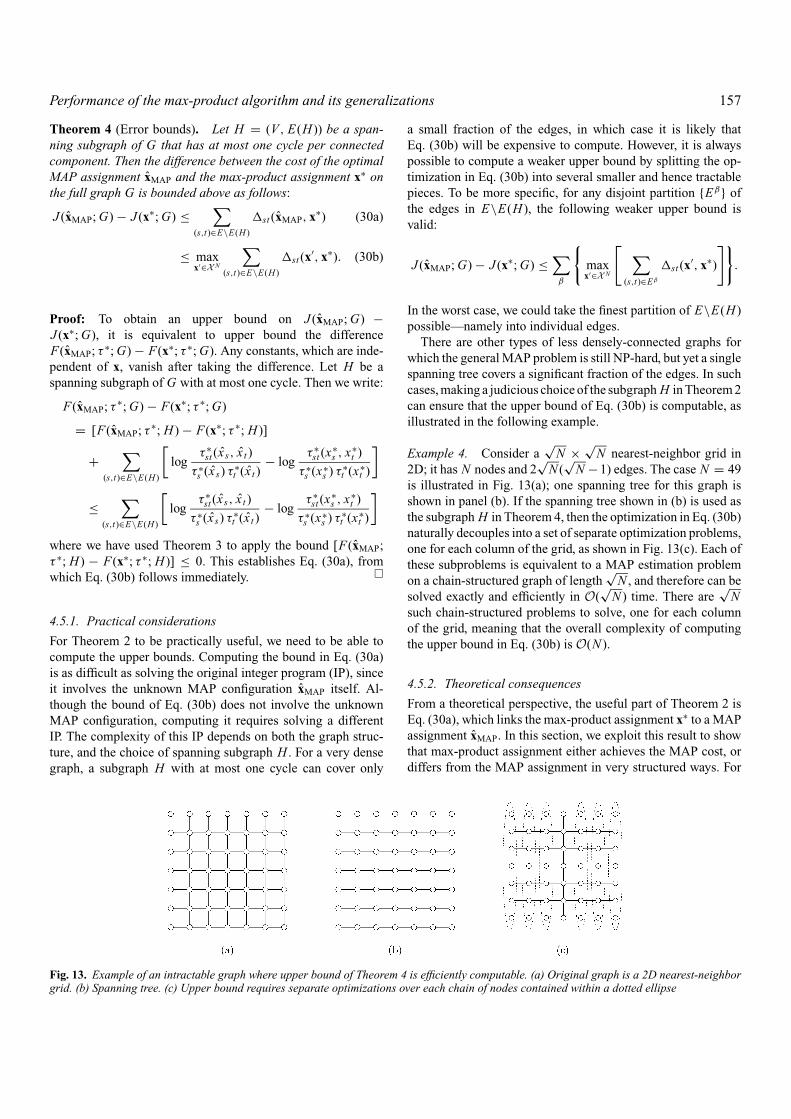
Fig. 12. Difference between node-induced subgraphs and general subgraphs. (a) Original graph is a 5 × 5 grid. (b) A node-induced subgraphwith a single cycle; nodes in gray are not part of the subgraph. (c) A spanning tree plus a single cycle. (d) A second spanning tree plus a singlecycle. Neither of the subgraphs in (c) or (d) are node-induced
Figure 12 illustrates the difference between the set of node-induced subgraphs to which Corollary 1 applies, and the largerset of subgraphs to which Theorem 3 applies. Shown in Fig. 12(a)is a graph with cycles, in this case a 5 × 5 grid. Panel (b) showsa particular node-induced subgraph; nodes in gray correspondto those not in the subgraph. Both Corollary 1 and Theorem 3apply to this subgraph. Panels (c) and (d) show two subgraphsto which Theorem 3 applies but Corollary 1 does not. Eachsubgraph consists of a spanning tree plus a single cycle. Notethat the vertex sets of each of these subgraphs are the full set V ,but their edge sets do not include every edge. Therefore, theyare not node-induced subgraphs, meaning that Corollary 1 nolonger applies.
Secondly, on the basis of Theorem 3, we can establish di-rectly a result that was first proved, using alternative methods,by Weiss (2000); this result is also a corollary of the Freemanand Weiss (2001) result from above.
Corollary 2 (Exactness on single cycles). Under Assump-tion 1, the max-product assignment is exact for a positive distri-bution on a graph containing at most one cycle.
4.5. Error bounds and consequences
In an integer programming problem, one way to measure theerror between the optimal assignment xMAP and a trial assign-ment x∗ is in terms of the difference between the optimal costJ (xMAP; G) and the cost J (x∗; G) associated with the approxi-mation. In this section, we show that our analysis enables us togive bounds on this error in the max-product assignment in astraight-forward manner. In addition, these bounds allow us toprove that the max-product assignment x∗ either agrees with aMAP configuration, or differs from any MAP configuration bya Hamming distance larger than a linear function of the graphgirth.
Let xMAP = {xs |s ∈ V } denote a MAP assignment, and letx∗ = {x∗
s |s ∈ V } denote the max-product assignment. We definethe following quantity to assess the discrepancy between xMAP
and x∗ on edge (s, t) ∈ E :
�st (xMAP, x∗) := logτ ∗
st (x s, x t )
τ ∗s (x s) τ ∗
t (x t )− log
τ ∗st (x
∗s , x∗
t )
τ ∗s (x∗
s ) τ ∗t (x∗
t ).
With this notation, we have:
Performance of the max-product algorithm and its generalizations 157
Theorem 4 (Error bounds). Let H = (V, E(H )) be a span-ning subgraph of G that has at most one cycle per connectedcomponent. Then the difference between the cost of the optimalMAP assignment xMAP and the max-product assignment x∗ onthe full graph G is bounded above as follows:
J (xMAP; G) − J (x∗; G) ≤∑
(s,t)∈E\E(H )
�st (xMAP, x∗) (30a)
≤ maxx′∈X N
∑(s,t)∈E\E(H )
�st (x′, x∗). (30b)
Proof: To obtain an upper bound on J (xMAP; G) −J (x∗; G), it is equivalent to upper bound the differenceF(xMAP; τ ∗; G) − F(x∗; τ ∗; G). Any constants, which are inde-pendent of x, vanish after taking the difference. Let H be aspanning subgraph of G with at most one cycle. Then we write:
F(xMAP; τ ∗; G) − F(x∗; τ ∗; G)
= [F(xMAP; τ ∗; H ) − F(x∗; τ ∗; H )]
+∑
(s,t)∈E\E(H )
[log
τ ∗st (x s, x t )
τ ∗s (x s) τ ∗
t (x t )− log
τ ∗st (x
∗s , x∗
t )
τ ∗s (x∗
s ) τ ∗t (x∗
t )
]
≤∑
(s,t)∈E\E(H )
[log
τ ∗st (x s, x t )
τ ∗s (x s) τ ∗
t (x t )− log
τ ∗st (x
∗s , x∗
t )
τ ∗s (x∗
s ) τ ∗t (x∗
t )
]
where we have used Theorem 3 to apply the bound [F(xMAP;τ ∗; H ) − F(x∗; τ ∗; H )] ≤ 0. This establishes Eq. (30a), fromwhich Eq. (30b) follows immediately. �
4.5.1. Practical considerations
For Theorem 2 to be practically useful, we need to be able tocompute the upper bounds. Computing the bound in Eq. (30a)is as difficult as solving the original integer program (IP), sinceit involves the unknown MAP configuration xMAP itself. Al-though the bound of Eq. (30b) does not involve the unknownMAP configuration, computing it requires solving a differentIP. The complexity of this IP depends on both the graph struc-ture, and the choice of spanning subgraph H . For a very densegraph, a subgraph H with at most one cycle can cover only
Fig. 13. Example of an intractable graph where upper bound of Theorem 4 is efficiently computable. (a) Original graph is a 2D nearest-neighborgrid. (b) Spanning tree. (c) Upper bound requires separate optimizations over each chain of nodes contained within a dotted ellipse
a small fraction of the edges, in which case it is likely thatEq. (30b) will be expensive to compute. However, it is alwayspossible to compute a weaker upper bound by splitting the op-timization in Eq. (30b) into several smaller and hence tractablepieces. To be more specific, for any disjoint partition {Eβ} ofthe edges in E\E(H ), the following weaker upper bound isvalid:
J (xMAP; G) − J (x∗; G) ≤∑
β
{maxx′∈X N
[ ∑(s,t)∈Eβ
�st (x′, x∗)
]}.
In the worst case, we could take the finest partition of E\E(H )possible—namely into individual edges.
There are other types of less densely-connected graphs forwhich the general MAP problem is still NP-hard, but yet a singlespanning tree covers a significant fraction of the edges. In suchcases, making a judicious choice of the subgraph H in Theorem 2can ensure that the upper bound of Eq. (30b) is computable, asillustrated in the following example.
Example 4. Consider a√
N × √N nearest-neighbor grid in
2D; it has N nodes and 2√
N (√
N −1) edges. The case N = 49is illustrated in Fig. 13(a); one spanning tree for this graph isshown in panel (b). If the spanning tree shown in (b) is used asthe subgraph H in Theorem 4, then the optimization in Eq. (30b)naturally decouples into a set of separate optimization problems,one for each column of the grid, as shown in Fig. 13(c). Each ofthese subproblems is equivalent to a MAP estimation problemon a chain-structured graph of length
√N , and therefore can be
solved exactly and efficiently in O(√
N ) time. There are√
Nsuch chain-structured problems to solve, one for each columnof the grid, meaning that the overall complexity of computingthe upper bound in Eq. (30b) is O(N ).
4.5.2. Theoretical consequences
From a theoretical perspective, the useful part of Theorem 2 isEq. (30a), which links the max-product assignment x∗ to a MAPassignment xMAP. In this section, we exploit this result to showthat max-product assignment either achieves the MAP cost, ordiffers from the MAP assignment in very structured ways. For

158 Wainwright, Jaakkola and Willsky
two strings a, b ∈ X N , we use dH (a, b) to denote the Hammingdistance:
dH (a, b) =N∑
i=1
δ(ai �= bi ). (31)
I.e., the Hamming distance is a count of the number of elementsin which a and b differ. Given a graph G, its girth is the numberof edges in its shortest cycle. The main result of this section isto show that the max-product assignment is either equivalent toa MAP assignment, or differs from it by a Hamming distancethat depends linearly on the girth. This result generalizes similarresults of the same flavor by Freeman and Weiss (2001).
Before proving this result, we require the following lemmas:
Lemma 5. Whenever dH {(x s, x t ), (x∗s , x∗
t )} ≤ 1, then�st (xMAP, x∗) ≤ 0.
Proof: If dH {(x s, x t ), (x∗s , x∗
t )} = 0, the statement is trivial.Otherwise, suppose without loss of generality that x s = x∗
s andx t �= x∗
t . Then we write:
�st (xMAP, x∗) = logτ ∗
st (x∗s , x t )
τ ∗s (x∗
s ) τ ∗t (x t )
− logτ ∗
st (x∗s , x∗
t )
τ ∗s (x∗
s ) τ ∗t (x∗
t )
= logτ ∗
st (x∗s , x t )
τ ∗t (x t )
− logτ ∗
st (x∗s , x∗
t )
τ ∗t (x∗
t )
≤ 0,
where we have used Lemma 4 to obtain the inequality. Thus,we have established that �st (xMAP, x∗) ≤ 0 for all x∗ withinHamming distance one of xMAP. �
Lemma 6. Given a graph G of girth g, define l(g) = 2g −(�g/2�+1). Here �g/2� denotes the floor of g/2 (i.e., its integralpart). Then any node induced subgraph G[S] with a number ofnodes |S| ≤ l(g) − 1 has at most one cycle.
Proof: See Appendix D. �
We now proceed to the main result of this section:
Corollary 3. For a graph G with girth g, the max-productassignment x∗ is either a MAP assignment (i.e., achieves theMAP value), or differs from any MAP assignment by a Hammingdistance of at least l(g) = 2g − �g/2� − 1.
Proof: Suppose that the max-product assignment x∗ is notequal to a MAP assignment; moreover, say it differs from a MAPassignment xMAP in a subset of vertices S with |S| ≤ l(g) − 1.By Lemma 6, the corresponding node-induced subgraph G[S]can have at most one cycle. Therefore, we can augment G[S]to a spanning subgraph H = (V, E(H )) that also contains atmost one cycle, and such that E(H ) contains the edge subsetE[S] = {(ui , u j ) ∈ E |ui , u j ∈ S}. Applying Eq. (30a) fromTheorem 4 to this subgraph, we obtain:
0 ≤ J (xMAP; G) − J (x∗; G) ≤∑
(s,t)∈E\E(H )
�st (xMAP, x∗). (32)
By construction, no edge (s, t) in E\E(H ) is of the form (ui , u j )for some ui , u j ∈ S. Therefore, if x∗ differs from xMAP only in el-ements within the set {x∗
u |u ∈ S}, then dH
{(x s, x t ), (x∗
s , x∗t )
} ≤1 for all (s, t) ∈ E\E(H ). In this case, applying Lemma 5 toEq. (32) yields that J (xMAP; G) = J (x∗; G), so that x∗ achievesthe MAP value. Otherwise, there must be at least one vertexs ∈ V \S (i.e., in addition to those in S) for which x∗
s �= x s .Therefore, x∗ must differ from xMAP by Hamming distance atleast |S| + 1. If |S| = l(g) − 1, then we are done; otherwise, wesimply augment S by adding the additional vertex s for whichx∗
s �= x s , and apply the same argument to this augmented set(using the fact that |S ∪ {s}| = |S| + 1 ≤ l(g) − 1.) This sameprocedure can be applied until |S| = l(g) − 1, at which pointwe will have established that x∗ is either equal to a MAP as-signment, or differs from any MAP assignment by Hammingdistance at least l(g). �
Remark. The Hamming distance bound of Corollary 3 is tightfor g = 3, in the sense that there exist graphs for which the boundis met with equality. For instance, consider the 4-node graphshown in Fig. 14(a); it has girth g = 3, and l(3) = 4. There existpotentials for this 4-node graph for which the MAP assignmentxMAP = [1111], whereas the max-product assignment is x∗ =[0000], so that dH {xMAP, x∗} = l(3).
We conclude this section by comparing Theorem 4 andCorollary 3 to some other approximation error results that ex-ist for integer programming problems. For certain special casesof the ferromagnetic Potts model, several researchers (Boykov,Veksler and Zabih 2001, Kleinberg and Tardos 1999) providedalgorithms that provide solutions with cost within a constantfactor of optimal. For the MAX-CUT problem, Goemans andWilliamson (1995) developed a randomized algorithm based ona semidefinite programming relaxation that also has a constantfactor guarantee (in expectation). Both of these problems are spe-cial cases of MAP problems on pairwise Markov random fields.Although we have not provided a constant factor guarantee, themax-product algorithm, and hence the results given here, aremore generally applicable to an arbitrary pairwise Markov ran-dom field. Moreover, rather than comparing solutions in termsof their costs, Corollary 3 either guarantees that a max-product
Fig. 14. Graphs with two minimal cycles, and girths g from 3 to 5.(a) In the case g = 3, adding a single node is sufficient to generatemultiple cycles of length 3. Note that in accordance with Lemma 6,l(3) = 6 − (1 + 1) = 4. (b) For a girth g = 4, we have l(4) =5 = 4 + 1, so that one node is again sufficient. (c) When g = 5, thenl(5) = 10 − 2 − 1 = 7, so that 2 additional nodes are required to formadditional cycles of length 5

Performance of the max-product algorithm and its generalizations 159
solution is MAP-optimal, or differs from any MAP solution interms of Hamming distance by a linear function of graph girth.An interesting direction for future research is to obtain tighterresults for when the max-product algorithm is restricted to morespecific problem classes.
5. Generalizations of max-product
Yedidia, Freeman and Weiss (2001) proposed extensions to thesum-product or belief propagation algorithm that entail operat-ing over higher order cliques. It is natural, then, to consider theanalogs of such generalizations for the max-product algorithm.As in the case of belief propagation, there are at least two rea-sons for doing so. First of all, the usual max-product algorithmapplies to a Markov random field (MRF) with pairwise maximalcliques. Of course, any MRF with higher order cliques can, inprinciple, be converted to a pairwise MRF defined on an aug-mented graph (see Freeman and Weiss 2001). Although the usualmax-product algorithm can be applied directly to this modifiedgraph, an alternative approach (described here) is to modify themax-product algorithm itself to handle higher-order cliques in adirect manner. Second, even for an MRF with pairwise maximalcliques, there may be good reasons to consider larger groupsof nodes over which to update—in particular, to obtain betterapproximations to the true MAP estimate. One way to constructsuch groupings is by adding edges to the graph, thereby form-ing an augmented graph with higher-order cliques. In fact, inthe limit of adding enough edges to the graph to triangulate it,performing reparameterization over the maximal cliques of thetriangulated graph is equivalent to applying the junction treealgorithm (Cowell et al. 1999, Dawid 1992), which yields theexact max-marginals and MAP estimate. However, for manygraphs, the process of triangulation leads to an explosion in theclique size, which means that the practical application of thisjunction tree algorithm is limited. Given the prohibitive cost ofthe junction tree algorithm, it is reasonable to consider partialtriangulations of graphs. Such structures arise in certain exten-sions to BP, such as the GBP updates of Yedidia, Freeman andWeiss (2001), which can be formulated as minimizing a costfunction (e.g., Kikuchi free energy) that is defined by a partiallytriangulated graph.
To date, the counterparts of these extensions have not beenexplored in the context of MAP estimation. Accordingly, thissection is devoted to the development and analysis of general-ized max-product updates. These updates involve reparameter-izing distributions that are defined by compatibility functionsover higher-order cliques. One way to discuss such updates isin terms of aggregated graphs, where new vertices are definedby aggregating sets of nodes of the original graph into clusters(e.g., as in Kikuchi approximations (Yedidia, Freeman and Weiss2001). The route that we pursue here is different, in that we for-mulate generalized max-product updates within the formalismof hypergraphs. Of particular importance to our developmentare acyclic hypergraphs, otherwise known as hypertrees, which
are essentially equivalent to junction trees (Cowell et al. 1999)We refer the reader to Berge (1989) and Bodlaender (1993) formore details on hypergraphs and hypertrees. Based on this set-up, we then introduce generalizations of the max-product algo-rithm that entail performing reparameterization over hypertrees.Finally, we discuss how our results on the ordinary max-productalgorithm have analogs for these generalizations.
5.1. Hypergraphs
Hypergraphs represent a natural generalization of graphs. Inparticular, a hypergraph GHYP = (V, E) consists of a vertexset V = {1, . . . , N }, and a set of hyperedges E , where each hy-peredge h is a particular subset of V (i.e., an element of thepower set of V ). The set of hyperedges can be viewed naturallyas a partially-ordered set, where the partial ordering is speci-fied by inclusion. More details on hypergraphs can be found inBerge (1989), whereas Stanley (1997) provides more informa-tion on partially-ordered sets (also known as posets).
Given two hyperedges g and h, one of three possibilities canhold:
(a) the hyperedge g is contained within h, in which case wewrite g < h.
(b) if h is contained within g, then we write h < g.(c) finally, if neither containment relation holds, then g and h
are incomparable.
We say that a hyperedge is maximal if it is not contained withinany other hyperedge.
With these definitions, an ordinary graph is a special case of ahypergraph, in which each maximal hyperedge consists of a pairof vertices (i.e., an ordinary edge of the graph). Note that forhypergraphs (unlike graphs), the set of hyperedges may include(a subset of) the individual vertices.
A convenient graphical representation of a hypergraph is interms of a diagram of its hyperedges, with (directed) edges rep-resenting the inclusion relations. Diagrams of this nature havebeen used by Yedidia, Freeman and Weiss (2001), who refer tothem as region graphs; other researchers (McEliece and Yildirim2002, Pakzad and Anantharam 2002) have used the term Hassediagram from poset terminology (Stanley 1997). Figure 15 pro-vides some simple graphical illustrations of hypergraphs. As aspecial case, any ordinary graph can be drawn as a hypergraph;in particular, panel (a) shows the hypergraph representation ofa single cycle on four nodes. Panel (b) shows a hypergraph thatis not equivalent to an ordinary graph, consisting of two hy-peredges of size three joined by their intersection of size two.Shown in panel (c) is a more complex hypergraph, to which wewill return in the sequel.
Given any hyperedge h, we define the sets of its descendantsand ancestors in the following way:
D(h) = {g ∈ E | g < h}, (33a)
A(h) = {g ∈ E | g > h}. (33b)

160 Wainwright, Jaakkola and Willsky
Fig. 15. Graphical representations of hypergraphs. Subsets of nodes corresponding to hyperedges are shown in rectangles, whereas the arrowsrepresent inclusion relations among hyperedges. (a) An ordinary single cycle graph represented as a hypergraph. (b) A simple hypergraph. (c) Amore complex hypergraph.
For example, given the hyperedge h = (1245) in the hypergraphin Fig. 15(c), we have A(h) = ∅ and D(h) = {(25), (45), (5)}.We use the notation D+(h) and A+(h) as shorthand for the setsD(h) ∪ h and A(h) ∪ h respectively.
5.2. Junction trees and hypertrees
Of particular importance are acyclic hypergraphs, which arealso known as hypertrees. In order to define these objects, werequire the notions of tree decomposition and running inter-section, which are well-known in the context of junction trees.More background on junction trees and running intersectioncan be found in Lauritzen (1996) or Cowell et al. (1999). Givena hypergraph GHYP, a tree decomposition is an acyclic graphin which the nodes are formed by the maximal hyperedges ofGHYP. Any intersection g ∩ h of two maximal hyperedges thatare adjacent in the tree is known as a separator set. The tree de-composition has the running intersection property if for any twonodes g and h in the tree, all nodes on the unique path joiningthem contain the intersection g ∩ h. A hypergraph is acyclic ifit possesses a tree decomposition with the running intersectionproperty. The width of an acyclic hypergraph is the size of thelargest hyperedge minus one; we use the term k-hypertree tomean a singly-connected acyclic hypergraph of width k.
As a simple illustration, a spanning tree of an ordinary graphis a 1-hypertree, because its maximal hyperedges (i.e., ordinaryedges) all have size two. As a second example, the hypergraphof Fig. 15(b) has maximal hyperedges of size three. This hyper-graph is acyclic with width two, since it is in direct correspon-dence with the junction tree on the two maximal hyperedgesand the single separator set (23). Figure 16 shows a more subtleexample. Again, it is easy to see that the hypergraph in panel (a)is in direct correspondence with a junction tree, and hence is awidth three hypertree. At first glance, the hypergraph illustratedin panel (b) might appear different, but in fact, it corresponds tothe same hypertree. From the junction tree view, the addition ofthe extra hyperedge (5) and links to (25) and (45) is superfluous.This issue will be clarified in Example 5(c).
5.3. Hypergraph-structured distributions
We now consider the role of hypergraphs and hypertrees in spec-ifying particular factorizations of distributions. Given a hyper-
graph GHYP, we consider a distribution specified as a productcompatibility functions over hyperedges:
p(x) = 1
Z
∏h∈E
ψh(xh). (34)
If this hypergraph is acyclic (and hence can be associated witha junction tree), then the well-known junction tree theorem(Cowell et al. 1999) guarantees that p can be factored as a prod-uct of max-marginals on maximal cliques divided by a productof max-marginals on separator sets in the junction tree.
Here we describe an alternative but equivalent factorizationin terms of the hypertree itself, which will be more convenientfor our purposes. First of all, given a hyperedge h ∈ E , wedefine the associated max-marginal over the subset of variablesxh = {xs | s ∈ h}:
µh(xh) = max{x′|x′
h=xh}p(x′). (35)
Next, we use these max-marginals to define a function ϕh asfollows:
ϕh(x) := µh(xh)∏g∈D(h) ϕg(xg)
, (36)
where D(h), as defined in Eq. (33a), is the set of descendants ofh. In terms of these quantities, the hypertree factorization itselfis very simple:
p(x) = 1
Z
∏h∈E
ϕh(xh). (37)
Fig. 16. Two different graphical representations of the same underlyinghypertree. (a) This diagram clearly corresponds to an acyclic hyper-graph. (b) This representation seems different, but in fact correspondsto the same hypertree. Hence hypertrees cannot be identified simply bythe absence (or presence) of cycles in poset diagrams
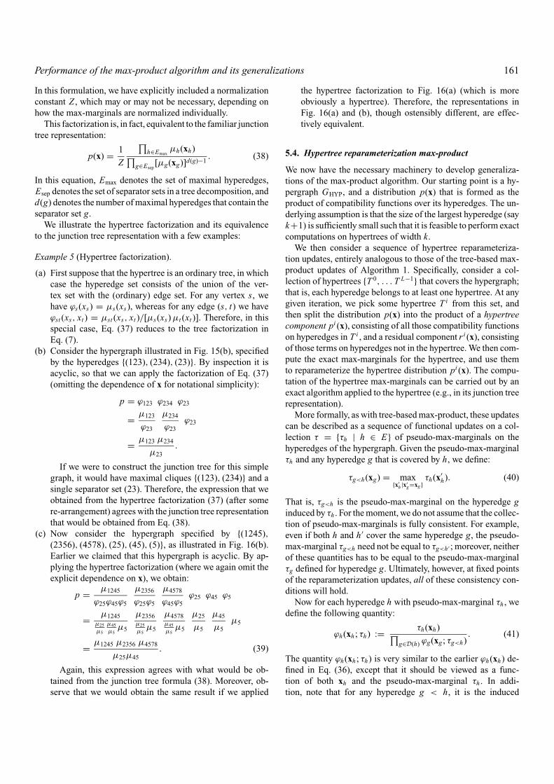
Performance of the max-product algorithm and its generalizations 161
In this formulation, we have explicitly included a normalizationconstant Z , which may or may not be necessary, depending onhow the max-marginals are normalized individually.
This factorization is, in fact, equivalent to the familiar junctiontree representation:
p(x) = 1
Z
∏h∈Emax
µh(xh)∏g∈Esep
[µg(xg)]d(g)−1. (38)
In this equation, Emax denotes the set of maximal hyperedges,Esep denotes the set of separator sets in a tree decomposition, andd(g) denotes the number of maximal hyperedges that contain theseparator set g.
We illustrate the hypertree factorization and its equivalenceto the junction tree representation with a few examples:
Example 5 (Hypertree factorization).
(a) First suppose that the hypertree is an ordinary tree, in whichcase the hyperedge set consists of the union of the ver-tex set with the (ordinary) edge set. For any vertex s, wehave ϕs(xs) = µs(xs), whereas for any edge (s, t) we haveϕst (xs, xt ) = µst (xs, xt )/[µs(xs) µt (xt )]. Therefore, in thisspecial case, Eq. (37) reduces to the tree factorization inEq. (7).
(b) Consider the hypergraph illustrated in Fig. 15(b), specifiedby the hyperedges {(123), (234), (23)}. By inspection it isacyclic, so that we can apply the factorization of Eq. (37)(omitting the dependence of x for notational simplicity):
p = ϕ123 ϕ234 ϕ23
= µ123
ϕ23
µ234
ϕ23ϕ23
= µ123 µ234
µ23.
If we were to construct the junction tree for this simplegraph, it would have maximal cliques {(123), (234)} and asingle separator set (23). Therefore, the expression that weobtained from the hypertree factorization (37) (after somere-arrangement) agrees with the junction tree representationthat would be obtained from Eq. (38).
(c) Now consider the hypergraph specified by {(1245),(2356), (4578), (25), (45), (5)}, as illustrated in Fig. 16(b).Earlier we claimed that this hypergraph is acyclic. By ap-plying the hypertree factorization (where we again omit theexplicit dependence on x), we obtain:
p = µ1245
ϕ25ϕ45ϕ5
µ2356
ϕ25ϕ5
µ4578
ϕ45ϕ5ϕ25 ϕ45 ϕ5
= µ1245µ25
µ5
µ45
µ5µ5
µ2356µ25
µ5µ5
µ4578µ45
µ5µ5
µ25
µ5
µ45
µ5µ5
= µ1245 µ2356 µ4578
µ25µ45. (39)
Again, this expression agrees with what would be ob-tained from the junction tree formula (38). Moreover, ob-serve that we would obtain the same result if we applied
the hypertree factorization to Fig. 16(a) (which is moreobviously a hypertree). Therefore, the representations inFig. 16(a) and (b), though ostensibly different, are effec-tively equivalent.
5.4. Hypertree reparameterization max-product
We now have the necessary machinery to develop generaliza-tions of the max-product algorithm. Our starting point is a hy-pergraph GHYP, and a distribution p(x) that is formed as theproduct of compatibility functions over its hyperedges. The un-derlying assumption is that the size of the largest hyperedge (sayk+1) is sufficiently small such that it is feasible to perform exactcomputations on hypertrees of width k.
We then consider a sequence of hypertree reparameteriza-tion updates, entirely analogous to those of the tree-based max-product updates of Algorithm 1. Specifically, consider a col-lection of hypertrees {T 0, . . . T L−1} that covers the hypergraph;that is, each hyperedge belongs to at least one hypertree. At anygiven iteration, we pick some hypertree T i from this set, andthen split the distribution p(x) into the product of a hypertreecomponent pi (x), consisting of all those compatibility functionson hyperedges in T i , and a residual component r i (x), consistingof those terms on hyperedges not in the hypertree. We then com-pute the exact max-marginals for the hypertree, and use themto reparameterize the hypertree distribution pi (x). The compu-tation of the hypertree max-marginals can be carried out by anexact algorithm applied to the hypertree (e.g., in its junction treerepresentation).
More formally, as with tree-based max-product, these updatescan be described as a sequence of functional updates on a col-lection τ = {τh | h ∈ E} of pseudo-max-marginals on thehyperedges of the hypergraph. Given the pseudo-max-marginalτh and any hyperedge g that is covered by h, we define:
τg<h(xg) = max{x′
h |x′g=xg}
τh(x′h). (40)
That is, τg<h is the pseudo-max-marginal on the hyperedge ginduced by τh . For the moment, we do not assume that the collec-tion of pseudo-max-marginals is fully consistent. For example,even if both h and h′ cover the same hyperedge g, the pseudo-max-marginal τg<h need not be equal to τg<h′ ; moreover, neitherof these quantities has to be equal to the pseudo-max-marginalτg defined for hyperedge g. Ultimately, however, at fixed pointsof the reparameterization updates, all of these consistency con-ditions will hold.
Now for each hyperedge h with pseudo-max-marginal τh , wedefine the following quantity:
ϕh(xh ; τh) := τh(xh)∏g∈D(h) ϕg(xg; τg<h)
. (41)
The quantity ϕh(xh ; τh) is very similar to the earlier ϕh(xh) de-fined in Eq. (36), except that it should be viewed as a func-tion of both xh and the pseudo-max-marginal τh . In addi-tion, note that for any hyperedge g < h, it is the induced

162 Wainwright, Jaakkola and Willsky
marginal τg<h that is used in the denominator of the definitionof Eq. (41).
With these definition, the collection τ specifies an alternativeparameterization of the original distribution p(x) on the fullhypergraph (which includes cycles in general) as follows:
p(x; τ ) = 1
Z (τ )
∏h∈E
ϕh(xh ; τh). (42)
Example 6.
(a) To illustrate these definitions, first consider the hypergraphrepresentation of an ordinary graph with pairwise maximalcliques, so that the hyperedge set consists of the union ofthe vertex set and (ordinary) edge set. Suppose that we aregiven a collection of pseudo-max-marginals τ = {τs, τst }.Then applying the definition in Eq. (41) yields, for a max-imal hyperedge h = (st) and size one hyperedge g = (s)respectively, the following expressions:
ϕst ( (xs, xt ); τst ) = τst (xs, xt )
maxx ′sτst (x ′
s, xt ) maxx ′tτst (xs, x ′
t )
(43a)
ϕs( xs ; τs) = τs(xs). (43b)
Consequently, in this special case, the parameterization ofEq. (42) reduces to the earlier “tree-like” decomposition inEq. (16).
(b) Now consider the hypergraph in Fig. 15(c). As an illustra-tion, let us compute ϕ1245(x; τ ) by applying Eq. (41). Forsimplicity in notation, we omit the dependence on x, and weassume that τ is locally consistent (so that we can ignore thedistinction between τg<h and τh). By doing so, we obtain:
ϕ1245 = τ1245
ϕ25 ϕ45 ϕ5
= τ1245 τ5
τ25 τ45.
In order to initialize the reparameterization updates, it is con-venient to assume that p(x) is defined by a product of compati-bility functions {ψh} over only maximal hyperedges h. There isno loss of generality in making this assumption, since we canalways absorb any compatibility function on a non-maximal hy-peredge into some maximal hyperedge that contains it. Given ahypertree T i with hypertree edge set E(T i ), the hypertree com-ponent pi (x; τ n) and residual component r i (x; τ n) are given,respectively, by the expressions:
pi (x; τ n) ∝∏
h∈E(T i )
ϕh
(xh ; τ n
h
)(44a)
r i (x; τ n) ∝∏
h∈E\E(T i )
ϕh
(xh ; τ n
h
). (44b)
With this set-up, the hypertree max-product algorithm consistsof the following steps:
Algorithm 2 (Reparameterization max-product on hyper-trees).
1. At iteration n = 0, initialize ϕh(x; τ 0h ) as follows:
ϕh
(x; τ 0
h
) ={
ψh(xh) if h is maximal
1 otherwise(45)
2. At iterations n = 1, 2, . . . , choose hypertree T i(n) with hy-peredge set Ei(n). Update pseudo-max-marginals as follows:
τ n+1h (xh) =
{max{x′|x′
h=xh} pi(n)(x′; τ n) if h ∈ Ei(n)
τ nh (xh) if h ∈ E\Ei(n)
(46)
Remarks. As a natural generalization of the tree reparame-terization form of ordinary max-product given in Algorithm 1,similar remarks are applicable to Algorithm 2. First of all, it isclear that the initialization4 given in Step 1 ensures that p(x; τ 0),as defined in Eq. (42), is equivalent to the original distributionp(x). Computing max-marginals on a given hypertree, asstipulated by Step 2, can be performed by any exact algorithmapplied to the hypertree.
If the updates of Algorithm 2 converge to a fixed point τ ∗,then we are guaranteed that for any of the hypertrees T i , theelements {τ ∗
h | h ∈ Ei } are a consistent set of max-marginalsfor the hypertree distribution pi (x; τ ∗). Therefore, given anyhyperedge h ∈ Ei and any other hyperedge g < h, the followinglocal consistency condition must hold:
τ ∗g (xg) = κτ ∗
g<h(xg) ≡ κ max{x′
h |x′g=xg}
τ ∗h (x′
h). (47)
Since every hyperedge h belongs to at least one of the hypertreesT 0, . . . , T L−1, we are guaranteed that Eq. (47) holds for everynested pair g < h of hyperedges in the full hypergraph. Givenany hypertree T with edge set E(T ), let us isolate those termscorresponding to edges in the hypertree so as to form a hypertree-structured distribution:
pT (x; τ ∗) ∝∏
h∈E(T )
ϕh(x; τ ∗h ).
By the junction tree theorem (Cowell et al. 1999), the localconsistency of {τ ∗
h | h ∈ E(T )} on all nested sets of hyper-edges implies that the pseudo-max-marginals {τ ∗
h | h ∈ E(T )}are equivalent to the exact max-marginals for the hypertree-structured distribution pT (x; τ ∗). The result that we have justestablished is the analog of Proposition 2(b), generalized to thecase of hypertrees.
Moreover, it should be clear that our other results on the ordi-nary max-product can be generalized to the hypertree reparam-eterization updates of Algorithm 2:
1. All of the iterates τ n , as well as any fixed point τ ∗, sim-ply specify a different parameterization of the distributionp(x). That is, the distribution p(x) is invariant, as stated inProposition 2(a) for ordinary max-product.
Performance of the max-product algorithm and its generalizations 163
2. As with our earlier analysis, we can define modified costfunctions that include only those terms corresponding to aparticular embedded hypergraph. We then can state and proveresults about the hypertree max-product assignment x∗, anal-ogous to those of Theorem 3.
3. Finally, it is possible to derive upper bounds on the differencebetween the log probability of the generalized max-productassignment and the log probability of the MAP assignment,similar to those of Theorem 4.
6. Discussion
We have developed a reparameterization framework for under-standing and analyzing the max-product algorithm, as well asa rich class of its generalizations. We have shown how thesealgorithms can be interpreted as seeking a particular factoriza-tion of a graph-structured distribution in terms of pseudo-max-marginals over (hyper)edges. These pseudo-max-marginals are,in fact, the exact max-marginals for a tree-structured graph, butapproximate for a general graph with cycles. The significanceof this max-marginal representation is in facilitating solution ofthe MAP estimation problem.
The reparameterization viewpoint gives some insight into thenature of max-product fixed points, and the associated max-product assignment. Key results include the fact the original dis-tribution is never altered by reparameterization updates, and thatany max-marginal fixed point is guaranteed to be consistent onevery tree of the graph. Our analysis also establishes the fact, notobvious for a graph with cycles, that fixed points of this naturealways exist for positive distributions. We exploited the repa-rameterization perspective to characterize the max-product as-signment, thereby generalizing earlier work (Freeman and Weiss2001, Weiss 2000). We also derived computable upper boundson the difference in the log probability of the MAP assignment,and that of the max-product assignment.
One open problem not addressed by our work is conver-gence of the max-product updates to one of the fixed pointsthat are guaranteed to exist. For a graph with cycles, neither theparallel message-passing updates nor the tree-based update ofAlgorithm 1 are guaranteed to converge, and indeed (at least incoding applications) failure of convergence appears to be thedominant error mode (e.g., Benedetto et al. 1996, Weiss 2000).Therefore, of interest are algorithms for finding fixed points withimproved or guaranteed convergence. In earlier work on the sum-product algorithm (Wainwright, Jaakkola and Willsky 2003),we found that more global tree-based updates, such as those ofAlgorithm 1, often have convergence properties superior to thoseof parallel message-passing updates. Preliminary experimentssuggest that such tree-based updates may also lead to improvedconvergence for the max-product case. Another direction worthexploring is the applicability of known techniques (e.g., Ortegaand Rheinboldt 2000) for solving fixed point equations.
This paper, in conjunction with our previous work on the sum-product or belief propagation algorithm (Wainwright, Jaakkola
and Willsky 2003) establishes that the notion of reparameteriza-tion is useful for analyzing a variety of algorithms for approxi-mate inference on graphs with cycles. More generally, approx-imate dynamic-programming algorithms, like sum-product andmax-product applied to graphs with cycles, have analogs for anycommutative semi-ring (Verdu and Poor 1987). In this context,it is interesting to speculate about analogs of our reparameteri-zation results for semi-rings more exotic than the sum-productand max-product cases.
Appendix A: Proof of Proposition 1
Since Lemma 1 shows that p(x; τ ∗) ≡ p(x), it is equivalent toprove that
τ ∗ab(xa, xb) = κ max
{x′|(x ′a ,x ′
b)=(xa ,xb)}p(x′; τ ∗) (48)
for each pair (a, b) ∈ E . Note that the equivalence of the pair-wise max-marginals implies the equivalence of the single nodemax-marginals (i.e., τ ∗
a = µ∗a).
Given any tree T , we can arbitrarily designate one node—saynode r—as the root. Every other node w ∈ V \{r} then has aunique parent, which we denote pa(w). See Fig. 5 of Section 3.1for an illustration. Using the parent-child relations, we decom-pose the distribution p(x; τ ∗) as follows:
p(x; τ ∗) = τ ∗r (xr )
∏w∈V \{r},v≡pa(w)
τ ∗vw(xv, xw)
τ ∗v (xv)
, (49)
where we have used v ≡ pa(w) as short-hand for the parent ofnode w.
If the tree T consists of a pair of nodes, then Eq. (48) is satisfiedtrivially. Otherwise, any tree on N ≥ 2 nodes has at least two leafnodes (Bollobas 1998), so that we can perform a leaf-strippingprocedure to prove Eq. (48) for the root node and one of itsneighbors. Consider a leaf node s with parent t , as illustratedin Fig. 5(c). From the decomposition in Eq. (49), the only partof p(x; τ ∗) that depends on xs is the quantity τ ∗
st (xs, xt )/τ ∗t (xt ).
From Eq. (15), we have:
maxx ′
s
τ ∗st (x
′s, xt )
τ ∗t (xt )
= κτ ∗
t (xt )
τ ∗t (xt )
= κ,
which is a constant for all xs ∈ X . Therefore, if we maximizep(x; τ ∗) over xs , then we obtain:
maxx ′
s
p(x; τ ∗) = τ ∗r (xr )
∏u∈V \{r,s},v≡pa(w)
τ ∗vw(xv, xw)
τ ∗v (xv)
× maxx ′
s
τ ∗st (x
′s, xt )
τ ∗t (xt )
∝ τ ∗r (xr )
∏w∈V \{1,s},v≡pa(w)
τ ∗vw(xv, xw)
τ ∗v (xv)
.
Thus, maximizing over xs eliminates node s, thereby leaving uswith the tree T \{s} with N − 1 nodes. We can proceed in thismanner until we reach the tree with a single edge—say (r, u)

164 Wainwright, Jaakkola and Willsky
where u is a neighbor of r . At this point, we will have shownthat
τ ∗ru(xr , xu) ∝ max
{x′|(x ′r ,x
′u )=(xr ,xu )}
p(x′; τ ∗), (50)
so that τ ∗ru is equivalent to the max-marginal µru . By varying
our choice of the leaf elimination ordering, we can arrange sothat u is any of the neighbors of node r . Finally, since our choiceof the root node was arbitrary, we can prove a statement of theform in Eq. (50) for any edge (a, b) ∈ E .
Appendix B: Proof of Theorem 2
B.1. Proof of Lemma 2
It is equivalent to show that each Lst is continuous. The func-tion Lst (·; k) is a maximum over the finite collection (namely,j ∈ X ) of a linear function of the log messages ζ. Conse-quently, it suffices to show that the maximum over a finitecollection is continuous. We first make note of the relationmax{a, b} = 1
2 [(a + b) + |a − b|], so that the maximum oftwo numbers is continuous. This relation can be extended tomaximizing over an arbitrary finite collection by the relationmax{a, b, c} = max{max{a, b}, c}.
B.2. Proof of Lemma 3
Let (s, t) be an arbitrary edge, and let i, j, k be arbitrary elementsof X . For compactness in notation, we define
φst ;s( j, k) := log ψst ( j, k) + log ψs( j)
Note that |φst ;s( j, k)| < ∞ for all j, k ∈ X since we haveassumed that the compatibility functionsψ were strictly positive.
Now for any ζ ∈ RD , we have
Lst (ζ; k) = maxj∈X
[φst ;s( j, k) +
∑u∈N (s)/t
ζus( j)
]
= maxj∈X
[φst ;s( j, i) +
∑u∈N (s)/t
ζus( j)
+ [φst ;s( j, k) − φst ;s( j, i)]
]
≤ maxj∈X
[φst ;s( j, i) +
∑u∈N (s)/t
ζus( j)
]
+ maxj∈X
[φst ;s( j, k) − φst ;s( j, i)]
= Lst (ζ; i) + maxj∈X
{φst ;s( j, k) − φst ;s( j, i)}
≤ Lst (ζ; i) + maxj∈X
|φst ;s( j, k) − φst ;s( j, i)|.
By interchanging k and i , we obtain for all ζ ∈ RD:
|Lst (ζ; k) − Lst (ζ; i)| ≤ maxj∈X
|φst ;s( j, k) − φst ;s( j, i)|
≤ maxk,i∈X
maxj∈X
|φst ;s( j, k) − φst ;s( j, i)|:= cst < ∞.
To complete the proof of the lemma, we write:
‖F(ζ)‖∞ = max(s,t)∈E
maxk∈X
|Fst (ζ; k)|
= max(s,t)∈E
maxk∈X
∣∣∣∣∣Lst (ζ; k) − 1
m
∑i∈X
Lst (ζ; i)
∣∣∣∣∣= max
(s,t)∈Emaxk∈X
∣∣∣∣∣ 1
m
∑i∈X
[Lst (ζ; k) − Lst (ζ; i)]
∣∣∣∣∣≤ max
(s,t)∈Emaxk∈X
1
m
∑i∈X
|Lst (ζ; k) − Lst (ζ; i)|
≤ max(s,t)∈E
cst
:= c < ∞.
Appendix C: Proof of Corollary 1
Let Sc = V \S denote the complement of S in the vertex set V .Then define a partition of the edge set into three disjoint subsetsas follows:
E(H [S]) := {(s, t) ∈ E | s, t ∈ S},E ′ := {(s, u) ∈ E | s ∈ S, u ∈ Sc},
E(H [Sc]) := {(u, v) ∈ E | u, v ∈ Sc}.In this notation, we have
F(x∗; τ ∗; H [S]) =∑s∈S
log τ ∗s (x∗
s )
+∑
(s,t)∈E(H [S])
logτ ∗
st (x∗s , x∗
t )
τ ∗s (x∗
s )τ ∗t (x∗
t ).
We now express F(x∗; τ ∗; G) in terms of F(x∗; τ ∗; H [S]) andsome extra terms:
F(x∗; τ ∗; G) = F(x∗; τ ∗; H [S]) +∑u∈Sc
log τ ∗u (x∗
u )
+∑
(u,v)∈E(Sc)
logτ ∗
us(x∗u , x∗
s )
τ ∗u (x∗
u )τ ∗s (x∗
s )
+∑
(s,u)∈E ′log
τ ∗su(x∗
s , x∗u )
τ ∗s (x∗
s )τ ∗u (x∗
u ). (51)
First of all, by Theorem 3, we have
F(x∗; τ ∗; H [S]) ≥ F(x; τ ∗; H [S]) (52)
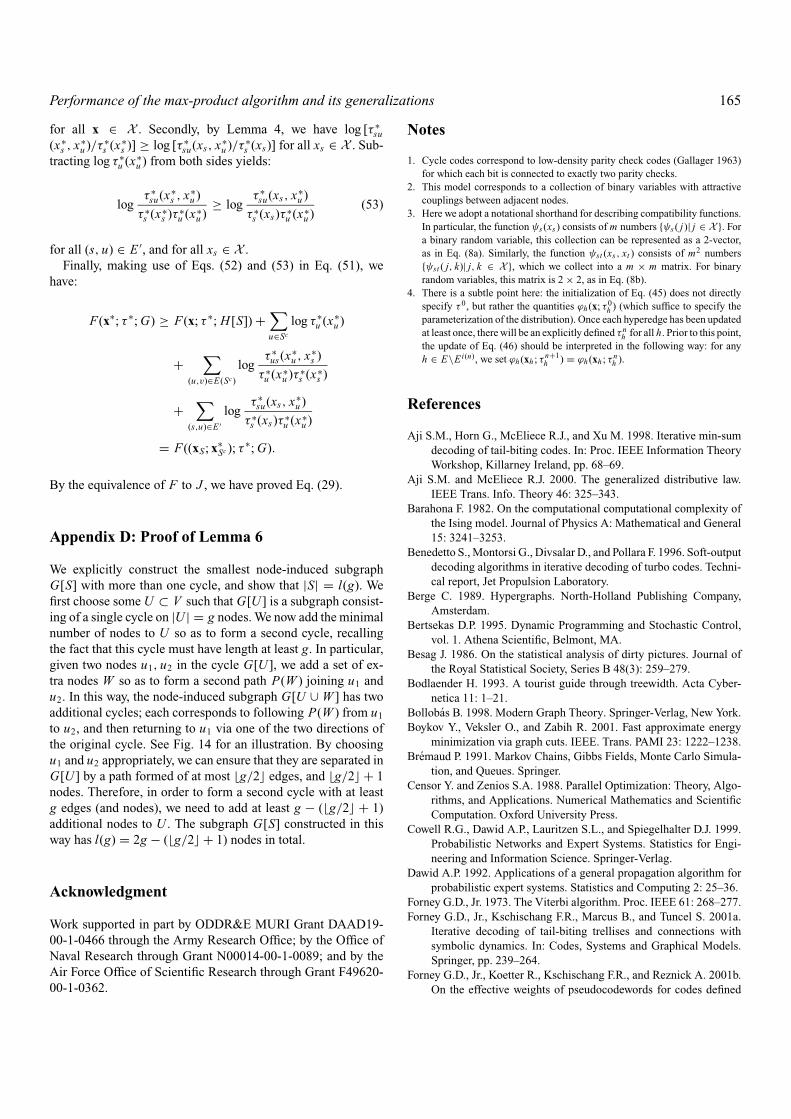
Performance of the max-product algorithm and its generalizations 165
for all x ∈ X . Secondly, by Lemma 4, we have log [τ ∗su
(x∗s , x∗
u )/τ ∗s (x∗
s )] ≥ log [τ ∗su(xs, x∗
u )/τ ∗s (xs)] for all xs ∈ X . Sub-
tracting log τ ∗u (x∗
u ) from both sides yields:
logτ ∗
su(x∗s , x∗
u )
τ ∗s (x∗
s )τ ∗u (x∗
u )≥ log
τ ∗su(xs, x∗
u )
τ ∗s (xs)τ ∗
u (x∗u )
(53)
for all (s, u) ∈ E ′, and for all xs ∈ X .Finally, making use of Eqs. (52) and (53) in Eq. (51), we
have:
F(x∗; τ ∗; G) ≥ F(x; τ ∗; H [S]) +∑u∈Sc
log τ ∗u (x∗
u )
+∑
(u,v)∈E(Sc)
logτ ∗
us(x∗u , x∗
s )
τ ∗u (x∗
u )τ ∗s (x∗
s )
+∑
(s,u)∈E ′log
τ ∗su(xs, x∗
u )
τ ∗s (xs)τ ∗
u (x∗u )
= F((xS; x∗Sc ); τ ∗; G).
By the equivalence of F to J , we have proved Eq. (29).
Appendix D: Proof of Lemma 6
We explicitly construct the smallest node-induced subgraphG[S] with more than one cycle, and show that |S| = l(g). Wefirst choose some U ⊂ V such that G[U ] is a subgraph consist-ing of a single cycle on |U | = g nodes. We now add the minimalnumber of nodes to U so as to form a second cycle, recallingthe fact that this cycle must have length at least g. In particular,given two nodes u1, u2 in the cycle G[U ], we add a set of ex-tra nodes W so as to form a second path P(W ) joining u1 andu2. In this way, the node-induced subgraph G[U ∪ W ] has twoadditional cycles; each corresponds to following P(W ) from u1
to u2, and then returning to u1 via one of the two directions ofthe original cycle. See Fig. 14 for an illustration. By choosingu1 and u2 appropriately, we can ensure that they are separated inG[U ] by a path formed of at most �g/2� edges, and �g/2� + 1nodes. Therefore, in order to form a second cycle with at leastg edges (and nodes), we need to add at least g − (�g/2� + 1)additional nodes to U . The subgraph G[S] constructed in thisway has l(g) = 2g − (�g/2� + 1) nodes in total.
Acknowledgment
Work supported in part by ODDR&E MURI Grant DAAD19-00-1-0466 through the Army Research Office; by the Office ofNaval Research through Grant N00014-00-1-0089; and by theAir Force Office of Scientific Research through Grant F49620-00-1-0362.
Notes
1. Cycle codes correspond to low-density parity check codes (Gallager 1963)for which each bit is connected to exactly two parity checks.
2. This model corresponds to a collection of binary variables with attractivecouplings between adjacent nodes.
3. Here we adopt a notational shorthand for describing compatibility functions.In particular, the function ψs (xs ) consists of m numbers {ψs ( j)| j ∈ X }. Fora binary random variable, this collection can be represented as a 2-vector,as in Eq. (8a). Similarly, the function ψst (xs , xt ) consists of m2 numbers{ψst ( j, k)| j, k ∈ X }, which we collect into a m × m matrix. For binaryrandom variables, this matrix is 2 × 2, as in Eq. (8b).
4. There is a subtle point here: the initialization of Eq. (45) does not directlyspecify τ 0, but rather the quantities ϕh (x; τ 0
h ) (which suffice to specify theparameterization of the distribution). Once each hyperedge has been updatedat least once, there will be an explicitly defined τ n
h for all h. Prior to this point,the update of Eq. (46) should be interpreted in the following way: for anyh ∈ E\Ei(n), we set ϕh (xh ; τ n+1
h ) = ϕh (xh ; τ nh ).
References
Aji S.M., Horn G., McEliece R.J., and Xu M. 1998. Iterative min-sumdecoding of tail-biting codes. In: Proc. IEEE Information TheoryWorkshop, Killarney Ireland, pp. 68–69.
Aji S.M. and McEliece R.J. 2000. The generalized distributive law.IEEE Trans. Info. Theory 46: 325–343.
Barahona F. 1982. On the computational computational complexity ofthe Ising model. Journal of Physics A: Mathematical and General15: 3241–3253.
Benedetto S., Montorsi G., Divsalar D., and Pollara F. 1996. Soft-outputdecoding algorithms in iterative decoding of turbo codes. Techni-cal report, Jet Propulsion Laboratory.
Berge C. 1989. Hypergraphs. North-Holland Publishing Company,Amsterdam.
Bertsekas D.P. 1995. Dynamic Programming and Stochastic Control,vol. 1. Athena Scientific, Belmont, MA.
Besag J. 1986. On the statistical analysis of dirty pictures. Journal ofthe Royal Statistical Society, Series B 48(3): 259–279.
Bodlaender H. 1993. A tourist guide through treewidth. Acta Cyber-netica 11: 1–21.
Bollobas B. 1998. Modern Graph Theory. Springer-Verlag, New York.Boykov Y., Veksler O., and Zabih R. 2001. Fast approximate energy
minimization via graph cuts. IEEE. Trans. PAMI 23: 1222–1238.Bremaud P. 1991. Markov Chains, Gibbs Fields, Monte Carlo Simula-
tion, and Queues. Springer.Censor Y. and Zenios S.A. 1988. Parallel Optimization: Theory, Algo-
rithms, and Applications. Numerical Mathematics and ScientificComputation. Oxford University Press.
Cowell R.G., Dawid A.P., Lauritzen S.L., and Spiegelhalter D.J. 1999.Probabilistic Networks and Expert Systems. Statistics for Engi-neering and Information Science. Springer-Verlag.
Dawid A.P. 1992. Applications of a general propagation algorithm forprobabilistic expert systems. Statistics and Computing 2: 25–36.
Forney G.D., Jr. 1973. The Viterbi algorithm. Proc. IEEE 61: 268–277.Forney G.D., Jr., Kschischang F.R., Marcus B., and Tuncel S. 2001a.
Iterative decoding of tail-biting trellises and connections withsymbolic dynamics. In: Codes, Systems and Graphical Models.Springer, pp. 239–264.
Forney G.D., Jr., Koetter R., Kschischang F.R., and Reznick A. 2001b.On the effective weights of pseudocodewords for codes defined
166 Wainwright, Jaakkola and Willsky
on graphs with cycles. In: Codes, Systems and Graphical Models.Springer, pp. 101–112.
Freeman W.T. and Pasztor E.C. 1999. Learning to estimate scenes fromimages. In: NIPS, vol. 11.
Freeman W.T. and Weiss Y. 2001. On the optimality of solutions ofthe max-product belief propagation algorithm in arbitrary graphs.IEEE Trans. Info. Theory 47: 736–744.
Frey B.J. and Koetter R. 2000. Exact inference using the attenuated max-product algorithm. In: Advanced Mean Field Methods: Theory andPractice. MIT Press.
Frey B.J., Koetter R., and Vardy A. 2001. Signal-space characterizationof iterative decoding. IEEE Trans. Info. Theory. 47: 766–781.
Fridman A. 2002. Topology-corrected belief revision in the ising model.Presented at Snowbird Learning workshop, Snowbird, UT.
Gallager R.G. 1963. Low-Density Parity Check Codes. MIT Press,Cambridge, MA.
Geman S. and Geman D. 1984. Stochastic relaxation, Gibbs distribu-tions, and the Bayesian restoration of images. IEEE Pat. Anal.Mach. Intell. 6: 721–741.
Goemans M.X. and Williamson D.P. 1995. Improved approximationalgorithms for maximum cut and satisfiability problems usingsemidefinite programming. Journal of the ACM 42: 1115–1145.
Grotschel M., Lovasz L., and Schrijver A. 1993. Geometric algo-rithms and combinatorial optimization. Springer-Verlag, Berlin,Germany.
Horn G. 1999. Iterative decoding and pseudocodewords. PhD thesis,California Institute of Technology.
Jordan M. (Ed.) 1999. Learning in graphical models. MIT Press,Cambridge, MA.
Kleinberg J. and Tardos E. 1999. Approximation algorithms for classi-fication problems with pairwise relationships: Metric labeling andMarkov random fields. In: IEEE Symp. Found. Comp. Science,pp. 14–24.
Lauritzen S.L. 1996. Graphical models. Oxford University Press,Oxford.
McEliece R.J. and Yildirim M. 2002. Belief propagation on partiallyordered sets. In: Gilliam D. and Rosenthal J. (Eds.), MathematicalTheory of Systems and Networks. Institute for Mathematics andits Applications.
Nilsson D. 1998. An efficient algorithm for finding the M most proba-ble configurations in a probabilistic expert system. Statistics andComputing 8: 159–173.
Ortega J.M. and Rheinboldt W.C. 2000. Iterative solution of nonlinearequations in several variables. Classics in Applied Mathematics.SIAM, New York.
Pakzad P. and Anantharam V. 2002. Iterative algorithms and free en-ergy minimization. In: Conference on Information Sciences andSystems.
Pearl J. 1988. Probabilistic reasoning in intelligent systems. MorganKaufman, San Mateo.
Stanley R.P. 1997. Enumerative combinatorics, vol. 1. Cambridge Uni-versity Press, Cambridge, UK.
Verdu S. and Poor H.V. 1987. Abstract dynamic programming modelsunder commutativity conditions. SIAM J. Control and Optimiza-tion 25(4): 990–1006.
Viterbi A. 1967. Error bounds for convolutional codes and an asymp-totically optimal decoding algorithm. IEEE Trans. Info. TheoryIT-13: 260–269.
Wainwright M.J., Jaakkola T.S., and Willsky A.S. 2003. Tree-basedreparameterization framework for analysis of sum-product andrelated algorithms. IEEE Trans. Info. Theory 49(5): 1120–1146.
Wainwright M.J. 2002. Stochastic processes on graphs with cycles:Geometric and variational approaches. PhD thesis, MIT.
Weiss. Y. 2000. Correctness of local probability propagation in graph-ical models with loops. Neural Computation 12: 1–41.
Wiberg N. 1996. Codes and decoding on general graphs. PhD thesis,University of Linkoping, Sweden.
Yedidia J.S., Freeman W.T., and Weiss Y. 2001. Generalized belief prop-agation. In: NIPS 13, MIT Press, pp. 689–695.
Related Documents