Tree Approximations of Dynamic Stochastic Programs

1

TREE APPROXIMATIONS OF DYNAMIC STOCHASTIC

PROGRAMS

R. MIRKOV AND G. PFLUG

Abstract. We consider a tree-based discretization technique utilizing conditional transporta-tion distance, which is well suited for the approximation of multi-stage stochastic programmingproblems, and investigate corresponding convergence properties. We explain the relation betweenthe approximation quality of the probability model and the quality of the solution.

Key words. stochastic programming, multistage, tree approximation, transportation distance,quality of solution

AMS subject classifications. 90C15

1. Introduction. Dynamic stochastic optimization models are an up to datetool of modern management sciences and can be applied to a wide range of problems,such as financial portfolio optimization, energy contracts, insurance policies, supplychains, etc. While one-period models look for optimal decision values (or decision vec-tors) based on all available information now, the multi-period models consider plannedfuture decisions as functions of the information that will be available later. Hence,the natural decision spaces for multi-period dynamic stochastic models, except for thefirst stage decisions, are spaces of functions. Consequently, only in some exceptionalcases solutions may be found by analytical methods, which include investigating thenecessary optimality conditions and solving a variational problem, i.e. only somefunctional equations have explicit solutions in observed spaces of functions. In thevast majority of cases, it is impossible to find a solution in this way, and we reach outfor a numerical solution. However, numerical calculation on digital computers maynever represent the underlying infinite dimensional function spaces. The way out ofthis dilemma is to approximate the original problem by a simpler, surrogate finitedimensional problem, which enables the calculation of the numerical solution.

As the optimal decision at each stage is a function of the random componentsobserved so far, the only way to reduce complexity is to reduce the range of therandom components. If the random component of the decision model is discrete (i.e.takes a finite and in fact only a few number of values), the variational problem isreduced to a vector optimization problem, which may be solved by well known vectoroptimization algorithms. The natural question that arises is how to reconstruct asolution of the basic problem out of the solution of the finite surrogate problem.

Since every finite valued stochastic process ξ1, . . . , ξT is representable as a tree,we deal with tree approximations of stochastic processes. There are two contradictinggoals to be considered. For the sake of the quality of approximation, the tree shouldbe large and bushy, while for the sake of computational solution effort, it shouldbe small. Thus the choice of the tree size is obtained through a compromise. Thebasic question in reaching this compromise is the assessment of the quality of theapproximation in terms of the tree size. It is the purpose of this paper to shed somelight on the relation between the approximation quality of the probability model forthe random components and the quality of the solution.

∗Department of Statistics and Decision Support Systems, University of Vienna, Universitatsstr.5/3, 1010 Vienna, Austria, email: [email protected], [email protected]

1

2 R. Mirkov and G. Pflug

Well known limiting results are available, which show that by increasing the size ofthe approximating tree, one eventually gets convergence of the optimal values and theoptimizing functions. Results in this direction were proved in [13], [14], etc. Recently,in [9] a stability result has been shown and an estimate of the approximation errorin terms of some distance between the continuous and the discrete models has beengiven.

Our approach is quite different. We start from the description of decision modelin terms of the systems dynamics functions, the constraint sets, and the objectivefunction. We formulate the whole problem in terms of distributions, as the resultsare independent from the choice of the probability space. Then we approximate thesedistributions in an appropriate setting by simpler, discrete distributions and comparethe decision functions and the optimal values in both cases.

In our distributional setup, there is no predefined probability space and thereforethere is no room for introducing other filtration than those which is generated by therandom process itself. Thus, we make the following assumption which is common instochastic optimization.

Assumption 1. No other information than the values of the scenario processξs, s ≤ t, is available to the the decision maker at time t, for t = 1, . . . , T . To put itdifferently, we assume that the decision xt is measurable with respect to σ-algebra Ft,which is the one generated by (ξ1, . . . , ξt).

Adopting this approach, there is no need to consider a filtration distance as donein [9].

A further consequence of the in-distribution setting is that we describe the deci-sions as functions of the random observations and not as functions defined on someprobability space. To be more precise, let ξt = (ξ1, . . . , ξt), t = 1, . . . , T , denotehistory of the random observations available up to time t. Then the t-th decisionis a function ξt 7→ xt(ξ

t) lying in some function space. Noticing that we want toapproximate a continuous probability distribution by a discrete one, we note thatthis function space should respect weak convergence i.e. if ξ(n) → ξ weakly, then alsox(ξ(n)) → x(ξ) weakly. Thus we must consider spaces of continuous functions or somesubspaces. In this paper, we work with the space of Lipschitz functions. The classof all Lipschitz functions on R

n determines the weak topology on all probabilities,which have the finite first moment. Moreover, the weakest topology making all inte-grals of Lipschitz functions continuous is generated by the well-known transportationdistance, which is convenient since it can be calculated or at least bounded in manyexamples.

A result of practical relevance to the decision maker will be shown under somestrong regularity assumptions: Suppose that the distance between the original prob-ability model and the approximate one is smaller than ε and that a δ0-solution ofthe approximate problem is found. Then one may construct out of it an δ-optimalsolution of the original problem. The relation between δ0, δ and ε is explicit (seeProposition 4.4). We measure the distance between the original probability modeland its discrete approximation by the conditional transportation distance, which isfiner than the usual unconditional transportation distance and accommodates for thedynamic character of the problem.

The paper is organized as follows. In Section 2 we describe the distance conceptsfor probability measures and for constraint sets. Section 3 contains the model and inSection 4 we state the approximation results. Two examples are treated in Section 5.In the Appendix we have collected some auxiliary results.

Tree Approximations of Dynamic Stochastic Programs 3

2. Preliminaries.

2.1. The Probability Model. Let ξ = (ξ1, . . . , ξT ) be a stochastic process withvalues in Ξ ⊂ R

nT , and u = (u1, . . . , uT ) its realization, with ut = (ut(1), . . . , ut(n)),for each t. Ξ is endowed with the metric

d(ut, vt) =

n∑

i=1

|χ(ut(i)) − χ(vt(i))|,

where χ is a strictly monotonic mapping R into R. (Ξ, d) is a complete separablemetric space such that Ξ = Ξ1 × · · · × ΞT , and Ξt ⊂ R

n, for each t. All metricsin all metric spaces appearing in this paper will be denoted by the same symbol d,since there is no danger of confusion. ut, t = 1, . . . , T − 1, denotes the history upto time t, i.e. ut = (u1, . . . , ut). Obviously, ut is an element of the metric spaceΞt = Ξ1 × · · · × Ξt ⊂ R

nt, which is endowed with the metric

d(ut, vt) =

t∑

s=1

d(us, vs).

For two Borel measures P , P on a metric space Ξ, we recall that the transportation(Wasserstein) distance dW between P and P is given by

dW (P, P ) = supf∈Lip1

(∫

f(u) dP (u) −∫

f(u) dP (u)

)

,

where u ∈ Ξ, and Lip1 is the set of all 1-Lipschitz function f , i.e.

|f(u) − f(v)| ≤ d(u, v), for all u, v ∈ Ξ.

The Wasserstein distance is related to the Monge’s mass transportation problem(see [20, p. 89]) through the following facts.

• Theorem of Kantorovich-Rubinstein

dW (P, P ) = infE[|Y − Y |]; where the joint distribution (Y, Y )is arbitrary, but the marginal distributions are fixed

such that Y ∼ P ; Y ∼ P

The infimum here is attained. The optimal joint distribution (Y, Y ) describeshow the mass P should be transported with minimal effort to yield the newmass P (see [20, Theorem 5.3.2 and Theorem 6.1.1]).

• For one-dimensional distributions, i.e. distributions on the real line endowedwith the Euclidean metric d(u, v) = |u − v|, having distribution functions G,resp. G, it holds that

dW (P, P ) =

∫

Ω

|G(u) − G(u)| du =

∫ 1

0

|G−1(u) − G−1(u)| du,

where G−1(u) = supv : G(v) ≤ u (see [25]).• If χ is a strictly monotonic function mapping R into R, defining the distance

d(u, v) = |χ(u) − χ(v)|, the pertaining transportation distance is

dW (P, P ) = dW (G χ−1, G χ−1) =

∫ 1

0

|χ(G−1(u)) − χ(G−1(u))| du.

By an appropriate choice of χ, the convergence of higher moments underdW -convergence may be ensured (see [16]).

4 R. Mirkov and G. Pflug

If random variables Y, Y have fixed marginal distributions P, P , it makes sense towrite

dW (P, P ) = dW (Y, Y ) = dW (G, G),(2.1)

as marginal distributions are on a par with the specifying random variables, and theirdistribution functions G, G, if they exist (see [27]).

The process ξ generates a Borel probability measure P on Ξ. This measure ischaracterized by its chain of regular conditional distributions:

P (A1 × · · · × AT )

=

∫

A1

· · ·∫

AT

PT (duT |uT−1) · · ·P3(du3|u2)P2(du2|u1)P1(du1)

=

∫

A1

· · ·∫

AT

PT (duT |(u1, . . . , uT−1)) · · ·P3(du3|(u1, u2))P2(du2|u1)P1(du1).

Here, Pt(At|ut−1) is the conditional probability of ξt ∈ At given the past ξt−1 =ut−1, t = 2, . . . , T , and P1 is the probability of ξ1 ∈ A1 (not conditional). Sincewe deal with complete separable metric spaces, the existence of regular conditionalprobabilities is ensured (see e.g. [6, Ch.4, Theorem 1.6]).

The following assumption is imposed on the measure P .Assumption 2. The conditional probabilities satisfy the Lipschitz condition, i.e.

dW (Pt(·|u), Pt(·|v)) ≤ Kt d(u, v)

for all u, v ∈ Ξt−1, and some constants Kt, for t = 2, . . . , T .Remark. The Assumption 2 is trivially satisfied if the process is independent.

For Markov processes, the condition in Assumption 2 reduces to

dW (Pt(·|ut−1), Pt(·|vt−1)) ≤ Kt d(ut−1, vt−1).

The ratio

supu,v

dW (P (·|u), P (·|v))

d(u, v)

is called the ergodic coefficient of the Markov transition P . If this coefficient is smallerthan one, geometric ergodicity holds. Ergodic coefficients were introduced in [4], andextensively applied to stochastic programming problems (see [15]).

Example. [Lipschitz Condition for Multivariate Normal Distribution] Assumethat the process ξ follows the multivariate normal distribution on R

T equipped withusual Euclidean metric with mean vector µ = µT and non-singular covariance matrixΣ = ΣT , where µt = (µ1, . . . , µt)

⊤, and Σt = (σi,j), i = 1, . . . , t, j = 1, . . . , t, fort = 1, . . . , T , are the main submatrices. It holds that

Σt =

[

Σt−1 σt

(σt)⊤ σt,t

]

t×t

.

Here σt, resp. (σt)⊤ denote the t-th column, resp. row vector of the covariance matrixΣt of the length t−1. According to [11, Theorem 13.1], the conditional distribution ofξt given the past realization ut−1 is normal with mean µt +(σt)⊤(Σt)−1(ut−1 −µt−1)and covariance σt,t − (σt)⊤(Σt−1)−1σt. The transportation distance satisfies

dW (Pt(·|ut−1), Pt(·|vt−1)) ≤ ‖(σt)⊤(Σt)−1‖∞ d(ut−1, vt−1),

Tree Approximations of Dynamic Stochastic Programs 5

for t = 2, . . . , T , and the constants Kt in Assumption 2 amount to ‖(σt)⊤(Σt)−1‖∞.Let P be some other probability measure that can also be dissected into the chain

of conditional probabilities. We introduce the notation

dW (P, P ) ≤ (ε1, . . . , εT )

if

dW (P1, P1) ≤ ε1

supu1

dW (P2(·|u1), P2(·|u1)) ≤ ε2

supu2

dW (P3(·|u2), P3(·|u2)) ≤ ε3

...

supuT−1

dW (PT (·|uT−1), PT (·|uT−1)) ≤ εT .

If P is the distribution of a stochastic process (ξ1, . . . , ξT ) with finite support,denote by Ξt the support of (ξ1, . . . , ξt). The conditional probabilities Pt(·|ut−1) areonly well defined, if ut−1 ∈ Ξt−1. If ut−1 /∈ Ξt−1, we set dW (Pt(·|ut−1), Pt(·|ut−1)) =0, which is the same as to say that the conditional probabilities of P are set equal tothose of P , for those values, which will not be taken by P with positive probability.

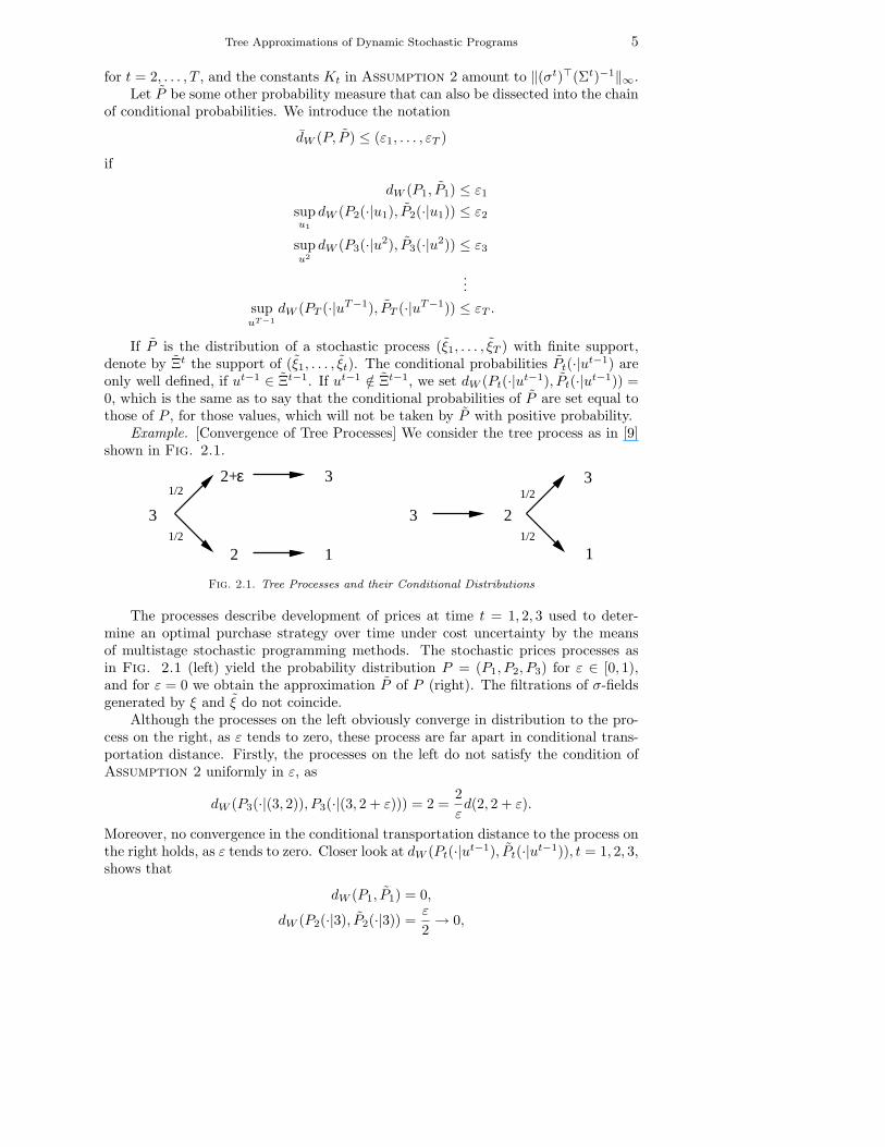
Example. [Convergence of Tree Processes] We consider the tree process as in [9]shown in Fig. 2.1.

3

2

3

1

2+ε

1/2

1/2

1/2

1/2

2

1

3

3

Fig. 2.1. Tree Processes and their Conditional Distributions

The processes describe development of prices at time t = 1, 2, 3 used to deter-mine an optimal purchase strategy over time under cost uncertainty by the meansof multistage stochastic programming methods. The stochastic prices processes asin Fig. 2.1 (left) yield the probability distribution P = (P1, P2, P3) for ε ∈ [0, 1),and for ε = 0 we obtain the approximation P of P (right). The filtrations of σ-fieldsgenerated by ξ and ξ do not coincide.

Although the processes on the left obviously converge in distribution to the pro-cess on the right, as ε tends to zero, these process are far apart in conditional trans-portation distance. Firstly, the processes on the left do not satisfy the condition ofAssumption 2 uniformly in ε, as

dW (P3(·|(3, 2)), P3(·|(3, 2 + ε))) = 2 =2

εd(2, 2 + ε).

Moreover, no convergence in the conditional transportation distance to the process onthe right holds, as ε tends to zero. Closer look at dW (Pt(·|ut−1), Pt(·|ut−1)), t = 1, 2, 3,shows that

dW (P1, P1) = 0,

dW (P2(·|3), P2(·|3)) =ε

2→ 0,

6 R. Mirkov and G. Pflug

but

dW (P3(·|(3, 2)), P3(·|(3, 2))) =1

2d(3, 1) = 1,

dW (P3(·|(3, 2 + ε)), P3(·|(3, 2 + ε))) = 0,

and supu2 dW (P3(·|u2), P3(·|(u2) = 1, i.e. it does not tend to 0.Associated to the process of observation ξt is the the process of decisions xt, where

xt are continuous mappings from Ξt into Rmt . On R

m, m =∑T

t=1 mt, we work withan appropriate distance d. We will assume that the optimal decisions are Lipschitzcontinuous. The next example shows why it is hopeless to get rid of assumptions onthe smoothness of the solutions.

Example. [Mean Absolute Deviation Regression] Let ξ1 be a uniform [0,1] variableand let ξ2, conditional on ξ1, have a normal distribution with mean ξ1/2 and variance1. Denote the distribution of (ξ1, ξ2) by P .

We want to solve

minx(ξ1)

EP (|x(ξ1) − ξ2|)(2.2)

where x(ξ1) is a measurable function of ξ1. Obviously the solution is

x(u) = u/2(2.3)

since the normal distribution is symmetric around zero. However, consider a sequenceof discrete measures P (n), converging weakly to P , and assume that these measures

sit on (ξ(n)1,i , ξ

(n)2,i ) with equal probability 1/n, such that all ξ

(n)1,i are distinct. Then the

solutions of

minx(ξ1)

1

n

n∑

i=1

(|x(ξ(n)1,i ) − ξ

(n)2,i |)(2.4)

would not converge to (2.3) in any sense.Smoothing techniques (sieve techniques) are used in nonparametric regression

for ensuring consistency. This technique would for fixed n search a solution x(·) ina smooth function space and gradually but slowly increase the function space as nincreases. The convergence rate depends on the degree of smoothness of the solution.To put this in terms of optimization, the approximate problem (2.4) is solved innonparametric statistics under an additional constraint of smoothness, which is notpresent in the original problem (2.2). Sieve techniques were introduced by [2], andare standard in nonparametric curve estimation (see for instance [7]). Only in rarecases, the additional smoothness condition is superfluous, because of strong shapeconditions ([21], [3]).

While in statistical applications one has to take the data as they are observed, onemay choose the approximating model in stochastic optimization. In other words, andthis is the approach we adopt here, one may choose the approximating model suchthat also the conditional probabilities of the approximations are close to the originalones. Let us see how this would solve the above nonparametric regression problem.Suppose we choose the points i/(n + 1), i = 1, . . . , n, each with probability 1/n, as agood approximation of the uniform distribution in the first component. Then chooseconditional on ξ1 = i/(n + 1) a discrete distribution which would come close to theoriginal normal distribution by a transportation distance not larger than ε. By doing

Tree Approximations of Dynamic Stochastic Programs 7

so, also the median would not differ more than ε, and by a simple linear interpolationbetween the points sitting at i/(n + 1) and at (i + 1)/(n + 1) we would have foundthe true regression line within a sup-norm distance of ε, too.

0 0.2 0.4 0.6 0.8 1−2

−1.5

−1

−0.5

0

0.5

1

1.5

2

0 0.2 0.4 0.6 0.8 1−2

−1.5

−1

−0.5

0

0.5

1

1.5

2

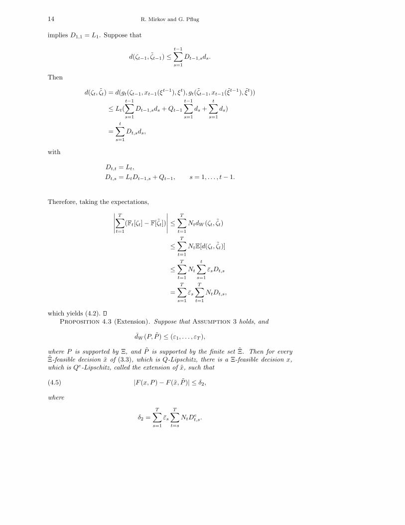
Fig. 2.2. Discrete approximations of the distribution of (ξ1, ξ2). The distribution on the left

is close in transportation distance, while the distribution on the right is in addition close in the

conditional transportation distance.

For an illustration, see Fig. 2.2. The left hand side shows a sample of the two-dimensional distribution which approximates the uniform distribution on the squarebased on the transportation distance. On the right hand side, we have chosen thex-coordinates as i/5, i = 1, . . . , 4, and only sampled the conditional distributions,i.e. it we have a tree-structured distribution, which approximates in addition someconditional distributions. In both cases we have shown the (linearly interpolated)solution of problem (2.2) as a dotted line.

2.2. The Projection Distance. Let B(r) = x ∈ Rm : d(0, x) ≤ r denote the

ball with diameter 2r in Rm. The projection distance dP,r between two closed, convex

sets A,B ⊆ Rm is defined as

dP,r(A,B) = supx∈B(r)

d(projA(x), projB(x)),

where projA(x) denotes the convex projection of the point x onto A. We allow r totake the value ∞ and set

dP (A,B) = dP,∞(A,B) = supx∈Rm

d(projA(x), projB(x)).

The projection distance is larger than the usual Hausdorff distance, which is

dH(A,B) = max(supx∈A

d(x,B), supx∈B

d(x,A)),

since

dH(A,B) = supx∈A∪B

d(projA(x), projB(x)) ≤ dP,∞(A,B).

8 R. Mirkov and G. Pflug

Example. [Projection and Hausdorff Distance] Let us show that there is no con-verse Lipschitz relation between dH and dP,∞. Consider in R

2 as set A the linesegment connecting [−1, ε] and [1,−ε], and as B the line segment connecting [−1,−ε]and [1, ε]. Here the Euclidean distance is used. A and B are closed convex sets withHausdorff distance dH(A,B). However, choosing the point x = (0, ε + 1/ε), one getsthat that the Hausdorff distance is smaller by an order than the projection distance,since dP (A,B) is hypotenuse of a triangle whose one leg is dH(A,B). More precisely,dP (A,B) = 2, and for ε ∈ (0, 1], dH(A,B) ≤ 2ε. In Fig. 2.3 the correspondingdistances for ε = 1/2 are represented by dotted lines.

ε

B

Aproj (x)A proj (x)B

x

Fig. 2.3. The Hausdorff and projection distance

Example. [Lipschitzian Property of Projection Distance] Let A1 and A2 be thehyperplanes

Ai = x : s⊤i x = wi ⊂ Rm, i = 1, 2.

Then

projAi(x) = x +

(wi − s⊤i x)si

‖si‖2,

and

‖projA1(x) − projA2

(x)‖ ≤

(

|w1| + ‖s1‖‖x‖ +|w2|‖s2‖

(‖s1‖ + ‖s2‖)) ‖s1 − s2‖

‖s1‖2+|w1−w2|

‖s2‖‖s1‖2

+‖x‖‖s1‖ + ‖s2‖‖s1‖

.

Suppose that s as well as w depend in a Lipschitz way on a parameter u. Thenthe set-valued mapping

u 7→ x ∈ B(r) : s(u)⊤x = w(u),

for r < ∞ is Lipschitz w.r.t. the projection distance dP,r, if ‖s(u)‖ and |w(u)| arebounded, and ‖s(u)‖ is bounded away from zero.

Tree Approximations of Dynamic Stochastic Programs 9

We utilize the projection distance in assumptions for the behavior of the constraintset.

Remark. Note that one could still use the weaker concept of the Hausdorff distancedH , which would put the results in a more classical setting, and allow the use of alreadyexisting results (for e.g. [23]). In that case there is no Lipschitz continuity and atmost (sub-)Holder continuity can be obtained. If X (z) denotes the constraint set (fordefinition and assumptions about constraint sets see Section 3), we say that dr issub-Holder continuous with modulus α, if for each r, there exists a constant Mr suchthat

dr(X (z),X (z)) ≤ Mr[d(z, z)]α,

where dr denotes the r-distance between closed, convex sets A and B, i.e.

dr(A,B) = supx∈B(r)

|d(x,A) − d(x,B)|.

In our case we obtain sub-Holder behavior of constraint sets with α = 1/2 and Mr =2√

r (cf. Lemma 6.1). Still, Holder property is weaker than Lipschitz, and does notpropagate well in multi-period situation. For this reason we stick to the projectiondistance.

3. Dynamic Decision Models. We represent the multistage dynamic decisionmodel as a state-space model. We assume that there is a state vector ζt, whichdescribes the situation of the decision maker at time t immediately before he mustmake the decision xt, for each t = 1, . . . , T , and its realization is denoted by zt. Theinitial state ζ0 = z0, which precedes the deterministic decision at time 0, is knownand given by ξ0. To assume the existence of such a state vector is no restriction atall, since we may always take the whole observed past and the decisions already madeas the state:

ζt = (xt−1, ξt), t = 1, . . . , T.

However, the vector of required necessary information for the future decisions is oftenmuch shorter.

The state variable process ζ = (ζ1, . . . , ζT ), with realizations z = (z1, . . . , zT ),is a controlled stochastic process, which takes values in a metric state space Z =Z1×· · ·×ZT . The control variables are the decisions xt, t = 1, . . . , T . The state ζt attime t depends on the previous state ζt−1, the decision xt−1 following it, and the lastobserved scenario history ξt with realization ut. A transition function gt describesthe state dynamics:

ζt = gt(ζt−1, xt−1, ξt), t = 1, . . . , T.(3.1)

At the terminal stage T , no decisions are made, only the outcome ζT = zT is observed.Note that ζt, as a function of the random variable ξt, is a random variable with

realization zt, which is a function of ut, the realization of ξt, for each t = 1, . . . , T .The decision x of the multistage stochastic problem is a vector of continuous

functions x = (x0, . . . , xT−1), where xt, t = 1, . . . , T − 1, maps Ξt to Rmt . We require

that the feasible decision xt at time t satisfies a constraint of the form

xt ∈ Xt(ζt), t = 1, . . . , T,

10 R. Mirkov and G. Pflug

where Xt are closed convex multifunctions with closed convex values. Let us nowdefine a Ξ-feasible decision.

Definition 3.1. We say that x is a Ξ-feasible decision, if the following is fulfilled.1. x0 ∈ X0(z0);2. u 7→ xt(u) is a continuous function Ξt → R

mt , t = 1, . . . , T − 1;3. if, for z0 given and (u1, . . . , uT ) ∈ Ξ, zt is recursively defined by

zt(ut) = gt(zt−1(u

t−1), xt−1(ut−1), ut), t = 1, . . . , T,

then

xt(ut) ∈ Xt(zt(u

t)), t = 1, . . . , T − 1.

X denotes the set of all Ξ-feasible decisions x = (x0, x1(ξ1), . . . , xT−1(ξ

T−1)).The objective to be minimized is

F (x, P ) :=T∑

t=1

Ft[ζt](3.2)

where Ft are version-independent probability functionals, i.e. mappings from a spaceof random variables on Zt to the real line, where the function values depend only onthe distribution and not on the concrete version of the random variable. Examplesfor version-independent probability functionals are the expectation, the moments, themean absolute deviation and all typical risk functionals used in finance.

Finally, we obtain the multistage problem in the state-dynamics representation:

minimize in x F (x, P ),subject to x ∈ X ,

(3.3)

i.e.

minimize in x

T∑

t=1

F[ζt],

subject to x ∈ X ,ζt is obtained through the recursion (3.1).

Its graphical representation is given in Fig. 3.1.

ζ

t=0 t=1 t=2

0

x0 x1 x2

21

1ξ ξ

2

t=T

T

TξxT−1

...

...z ζ ζ

Fig. 3.1. Multi-Stage State-Dynamics Decision Process

Since the decisions xt of the multistage problem are functions of the states ζt,the optimal set of decisions is expressed as a set of functions xt = xt(ζt). Theproblem (3.3) is a variational problem, and explicit solution methods for it exist onlyin exceptional cases.

Tree Approximations of Dynamic Stochastic Programs 11

Remark. The existence of continuous solutions (or better continuous selectionsfrom the arg min-sets) in our setting requires further consideration. We just men-tion here that such a type of result is contained in [22], where it is shown that un-der continuity and convexity assumptions, the existence of continuous measurablenon-anticipative solutions is guaranteed, if the probability measure is laminary. Theproperty of laminarity is close to our Assumption 2, but is not implied by it. Tobe more precise, assume that St(u

t) is the support of the conditional distribution of(ξt+1, . . . , ξT ) given ξt = ut. It is not difficult to see that Assumption 2 implies thatut 7→ St(u

t) is a closed-valued, lower semicontinuous multifunction. If ut 7→ St(ut) is,

in addition, continuous (in the Painleve-Kuratowski sense) for t = 1, . . . , T , then thedistribution of ξ is laminary.

We state now a set of smoothness and dependence assumptions for the model.Assumption 3. Let for each t = 1, . . . , T , and some real constants Lt,Mt, Nt,

the following holds.• The functions gt satisfy

d (gt(z, x, u), gt(z, x, u)) ≤ Lt (d(z, z) + d(x, x) + d(u, u)) ,

for z, z with values in Zt−1, x ∈ Xt−1(z), x ∈ Xt−1(z), u, u ∈ Ξt.• The constraints are described by closed convex sets Xt(z), which depend in a

Lipschitz way on z, such that

dP,r(Xt(z),Xt(z)) ≤ Mtd(z, z),

for z, z with values in Zt, where dP,r denotes the projection distance betweenclosed convex sets. Here r is finite, if we know that the solutions lie in B(r),otherwise we set r = ∞.

• The version-independent probability functionals Ft satisfy

|Ft(ζ) − Ft(ζ)| ≤ NtdW (ζ, ζ),

where dW is the Wasserstein distance, and ζ, ζ with distributions on Zt.In view of (2.1), we write dW (ζ, ζ) instead of dW (P, P ), for some adequate prob-

ability measure P .Remark. The second Lipschitz condition of Assumption 3 assures that Xt(z) is a

non-empty set, for all z with values in Zt, for t = 1, . . . , T , i.e. no induced constraintsare allowed.

Assumption 4. The components ξt = (ξt(1), . . . , ξt(n)) of the random process ξare conditionally independent given the past ξt−1.

This assumption is not as strong as it sounds. In the dynamics

ζt = gt(ζt−1, xt−1, ξt−1, ξt(1), . . . , ξt(n)),

we may assume that the risk factors (ξt(1), . . . , ξt(n)) are conditionally independentgiven the past ξt−1, otherwise we transform the originally dependent components intoconditionally independent ones, and reformulate the transition function gt accordingly.

4. Approximations. Instead of the original problem (3.3) we consider a treeprocess (ξ1, . . . , ξT ) with distribution P and support Ξ. The decision based on theapproximation is Ξ-feasible. We assume that Ξ ⊂ Ξ

Definition 4.1. We say that x is a Ξ-feasible decision, if the following is fulfilled.1. x0 ∈ X0(z0);

12 R. Mirkov and G. Pflug

2. u 7→ xt(u) is a continuous function Ξt → Rmt , t = 1, . . . , T − 1;

3. if, for z0 given and (u1, . . . , uT ) ∈ Ξ, zt is recursively defined by

zt(ut) = gt(zt−1(u

t−1), xt−1(ut−1), ut), t = 1, . . . , T,

then

xt(ut) ∈ Xt(zt(u

t)), t = 1, . . . , T − 1.

X denotes the set of all Ξ-feasible decisions x = (x0, x1(ξ1), . . . , xT−1(ξ

T−1)).This yields the approximate problem

minimize in x F (x, P ),

subject to x ∈ X ,(4.1)

i.e.

minimize in xT∑

t=1

F[ζt],

subject to x ∈ X ,

ζt is obtained through the recursion (3.1).

Remark. We do not propose the use of any random sampling technique to con-struct the tree, but rather to control the transportation distance between the condi-tional distributions of the original problem and of the approximating tree. In partic-ular, the first approximation is obtained by making dW (P1, P1) small. This amountsto finding a good solution of a facility location problem (see [10]). Suppose that n1

points u1(1), . . . , u1(n1) on the first stage have been selected. Then we choose the con-

ditional probabilities P (·|ui(j)) such that they are close to P (·|ui(j)), j = 1, . . . , n1,again in transportation distance. This procedure is then repeated through all stages.

The next two propositions tell us how to arrive from a solution of the originalproblem to a solution of the approximate problem, and vice versa. We assume thatboth problems have Lipschitz solutions. In Section 5, we give examples, which showthat the Lipschitz property of the solution is quite natural in problems from financeand supply chain management. In inventory control problem the solution is Lipschitzcontinuous if the dependence between the under-/over-shooting quantity and costs islinear, which is typically fulfilled.

Proposition 4.2 (Restriction). Suppose that Assumption 3 holds, and

dW (P, P ) ≤ (ε1, . . . , εT ),

where P is supported by Ξ, and P is supported by the finite set Ξ. Then every Ξ-feasible decision x, which is Q-Lipschitz, is also Ξ-feasible, and we have that

|F (x, P ) − F (x, P )| ≤ δ1,(4.2)

with

δ1 =

T∑

s=1

εs

T∑

t=s

NtDt,s,

Tree Approximations of Dynamic Stochastic Programs 13

where

εs =s∑

i=1

εi

s∏

j=i+1

Kj ,(4.3)

and, for Q = (Q0, . . . , QT−1), the constants Ds,t fulfill the recursion

Dt,t = Lt,

Dt,s = LtDt−1,s + Qt−1, s = 1, . . . , t − 1.(4.4)

Proof. It is evident that every Ξ-feasible decision is automatically Ξ feasible.Under Assumption 2, one may construct for every t stochastic processes ξt(u),

u ∈ Ξt−1, and ξt(u), u ∈ Ξt−1, sitting for every t on independent (product) probabilityspaces such that

(i) ξt(u) has distribution Pt(·|u);(ii) for all u, v ∈ Ξt−1,

E[d(ξt(u), ξt(v))] = dW (Pt(·|u), Pt(·|v)) ≤ Kt d(u, v);

(iii) if u ∈ Ξt−1, then

E[d(ξt(u), ξt(u))] = dW (Pt(·|u), Pt(·|u)) ≤ εt.

The construction of the processes is based on the following. Since the componentsξt = (ξt,1, . . . , ξt,n) of the process ξ are conditionally independent (Assumption 4),their conditional distribution functions at (y1, . . . , yn) given ut−1 = u can be writtenas Gt,u,1(y1), . . . , Gt,u,n(yn). Then ξt(u) is defined as

ξt(u) = (G−1t,u,1(U1), . . . , G

−1t,u,n(Un)).

where U1, . . . , Un are i.i.d. Uniform[0,1]. By this construction, (i) and (ii) are fulfilled.As to (iii), recall the Theorem of Kantorovich-Rubinstein, and notice that the infimumis attained. This joint ”minimal” distribution can be glued to the distribution Pt(·|u),to entail (iii) (see [26, Lemma 7.6]).

The processes ξt and ξt then appear as compositions ξt(ξt−1(· · · (ξ1) · · ·)), resp.ξt(ξt−1(· · · (ξ1) · · ·)). We show that E[d(ξt, ξt)] ≤ εt. Obviously, E[d(ξ1, ξ1)] ≤ ε1.Suppose that it is already shown that E[d(ξt−1, ξt−1)] ≤ εt−1. Then

εt = E[d(ξt(ξt−1), ξt(ξt−1))

≤ E[d(ξt(ξt−1), ξt(ξt−1))] + E[d(ξt(ξt−1), ξt(ξt−1))]

≤ Ktεt−1 + εt,

leading to (4.3).Now we argue point-wise for a specific ω in the standard probability space [0, 1]N

with Lebesgue measure, which we have constructed. All following calculation are donefor this specific ω. We use the fact that a point-wise argument implies a distributionalresult.

Set d(ξt, ξt) = dt and d(ξt, ξt) = dt =∑t

s=1 ds.

d(ζ1, ζ1) = d(g1(z0, x0, ξ1), g1(z0, x0, ξ1)) ≤ L1d1,

14 R. Mirkov and G. Pflug

implies D1,1 = L1. Suppose that

d(ζt−1, ζt−1) ≤t−1∑

s=1

Dt−1,sds.

Then

d(ζt, ζt) = d(gt(ζt−1, xt−1(ξt−1), ξt), gt(ζt−1, xt−1(ξ

t−1), ξt))

≤ Lt(

t−1∑

s=1

Dt−1,sds + Qt−1

t−1∑

s=1

ds +

t∑

s=1

ds)

=t∑

s=1

Dt,sds,

with

Dt,t = Lt,

Dt,s = LtDt−1,s + Qt−1, s = 1, . . . , t − 1.

Therefore, taking the expectations,

∣

∣

∣

∣

∣

T∑

t=1

(Ft[ζt] − F[ζt])

∣

∣

∣

∣

∣

≤T∑

t=1

NtdW (ζt, ζt)

≤T∑

t=1

NtE[d(ζt, ζt)]

≤T∑

t=1

Nt

t∑

s=1

εsDt,s

=

T∑

s=1

εs

T∑

t=1

NtDt,s,

which yields (4.2).Proposition 4.3 (Extension). Suppose that Assumption 3 holds, and

dW (P, P ) ≤ (ε1, . . . , εT ),

where P is supported by Ξ, and P is supported by the finite set Ξ. Then for everyΞ-feasible decision x of (3.3), which is Q-Lipschitz, there is a Ξ-feasible decision x,which is Qe-Lipschitz, called the extension of x, such that

|F (x, P ) − F (x, P )| ≤ δ2,(4.5)

where

δ2 =

T∑

s=1

εs

T∑

t=s

NtDet,s.

Tree Approximations of Dynamic Stochastic Programs 15

The ε’s are given by (4.3) and, for Qe = (Qe0, . . . , Q

eT−1), the constants Qe

t , and Des,t

fulfill the recursions

Qet = Qt + Mt

t−1∑

s=1

Det−1,s,

Det,t = Lt,

Det,s = LtD

et−1,s + Qe

t−1, s = 1, . . . , t − 1.

Proof. Again, we construct the processes ξ and ξ on the standard probabilityspace [0, 1]N. As in Proposition 4.2, the argumentation is point-wise for a specificω in this probability space.

Set d(ξt, ξt) = dt, and d(ξt, ξt) = dt =∑t

s=1 ds.

Let x be a Q-Lipschitz, Ξ-feasible family of decisions. By the Extension Theorem(Theorem 6.2), we may extend these functions to a family of functions xe definedon the whole Ξ with the same Lipschitz constant.

It may happen that the xe functions are not feasible. We have to make themfeasible in a recursive way, starting with xe

1, then xe2, and so on.

Let ζ1(ξ1) = g1(z0, x0, ξ1). Then

d(ζ1(ξ1), ζ1(ξ1)) ≤ L1d1.

Let now

x1(ξ1) := projX (z1)(xe1(ξ1)).

Since X (z1(u)) is (M1L1)-Lipschitz and xe1 is Q1-Lipschitz, we have by Lemma 6.3

in §6, that x1 is (Q1 + M1L1)-Lipschitz and that

d(ζ2, ζ2) ≤ L2(L1d1 + (Q1 + M1L1)d1 + d2).

This argument gets recursively iterated as in the proof of Proposition 4.2, leadingto the indicated sequences of constants, and finally to (4.5).

Remark. There are various variants of the Proposition 4.3, for instance if normsare replaced by equivalent ones or if the process ξ is Markovian. For particular models,much finer and better estimates may be found.

Recall the notion of δ-optimal solutions. In the given setting, they belong to

δ- arg minx

F (x, P ) = x ∈ X |F (x, P ) ≤ infx

F (x, P ) + δ, resp.

δ- arg minx

F (x, P ) = x ∈ X |F (x, P ) ≤ infx

F (x, P ) + δ.

The concept of approximately optimal solutions offers us more flexible frameworkas the δ- arg min-mappings satisfy the Lipschitz continuity under some additionalconditions, i.e. F has to be proper, lower semicontinuous and convex (cf. [23, Ch.7J]).

Based on the statements above, we have the following result.Proposition 4.4. Suppose that Assumption 3 holds, and

dW (P, P ) ≤ (ε1, . . . , εT ),

where P is supported by Ξ, and P is supported by the finite set Ξ, and the approxi-mation has been chosen so that the values of δ1 = δ1(ε) and δ2 = δ2(ε) are given, for

16 R. Mirkov and G. Pflug

ε = (ε1, . . . , εT ). If x∗ is a δ0-optimal solution of the approximate problem (4.1), thenits extension x∗ is a (δ0 + δ1 + δ2)-optimal solution of the basic problem (3.3).

Proof. Let y∗ be a solution of the basic problem (3.3). Since x∗ is a δ0-solutionof the approximate problem (4.1),

F (x∗, P ) − δ0 ≤ infx

F (x, P ) ≤ F (y∗, P )

and by virtue of (4.2) and (4.5), we have

|F (y∗, P ) − F (y∗, P )| ≤ δ1

|F (x∗, P ) − F (x∗, P )| ≤ δ2.

This implies

F (y∗, P ) ≥ F (y∗, P ) − δ1

≥ F (x∗, P ) − δ0 − δ1

≥ F (x∗, P ) − δ0 − δ1 − δ2.

Corollary 4.5. Suppose that Assumption 3 holds, and

dW (P, P ) ≤ (ε1, . . . , εT ),

where P is supported by Ξ, and P is supported by the finite set Ξ, and the approx-imation has been chosen so that the values of δ1 = δ1(ε) and δ2 = δ2(ε) are given.If x∗ is the solution of the approximate problem (4.1), then its extension x∗ is a(δ1 + δ2)-solution of the basic problem (3.3).

Proof. Choosing δ0 = 0 and applying the Proposition 4.4 we get the statementimmediately.

5. Examples.

5.1. Multi-Stage Portfolio Optimization. Consider an investor, who hasinitial capital C and wants to invest in m different assets. The price of one unit ofasset i at time t, t = 1, . . . , T , is the random quantity ξt,i. At starting time 0, theprices ξ0,i are deterministic.

Let ξt = (ξt,1, . . . , ξt,m)⊤ be the vector price process. The optimization problemis to maximize the acceptability of the final wealth under the self-financing constraint,i.e.

maximize in x A[x⊤T−1ξT ],

subject to x⊤0 ξ0 = C,

x⊤t−1ξt = x⊤

t ξt, t = 1, . . . , T − 1,

(5.1)

where A denotes some acceptability functional (see [1], [18]). By introducing thewealth wt at time t as

wt = x⊤t−1ξt,

and defining the state as

ζt =

(

wt

ξt

)

,

Tree Approximations of Dynamic Stochastic Programs 17

one gets the dynamics

(

wt

ξt

)

=

(

x⊤t−1ξt

ξt

)

, t = 1, . . . , T.

The constraint sets are

Xt(ζt) = xt : x⊤t ξt = wt, t = 1, . . . , T.

Under the realistic assumption that the returns are bounded from above and frombelow

0 < a ≤ ξt,i ≤ b < ∞,

this dynamics is Lipschitz in the sense of Assumption 2, since x must be boundeddue the the initial budget constraint. In addition, the constraint sets are Lipschitz,see Example on p. 8.

The tree approximation of (5.1) is given by

maximize in x A[x⊤T−1ξT ],

subject to x⊤0 ξ0 = C,

x⊤t−1ξt = x⊤

t ξt, t = 1, . . . , T − 1.

Probability functionals, which are Lipschitz w.r.t. the transportation distance inR include the expectation, the mean absolute deviation, distortion functionals (andtherefore the average value-at-risk as a special case), and linear combinations of them([17]).

As illustration, let us consider the Average Value-at-Risk corrected expectation([24])

A[z] := E[z] − βAV @Rα(z), 0 ≤ β ≤ 1,

where AV @Rα(z) is defined by (6.1).By

∣

∣

∣

∣

a − 1

αE([z − a]−) − a +

1

αE[[z − a]−]

∣

∣

∣

∣

≤ 1

αE[|z − z|]

one sees that AV @Rα is Lipschitz w.r.t. the transportation metric. The Lipschitzconstant of E[z] − β AV @Rα(z) is 1 + β/α.

5.2. Multi-Stage Inventory Control Problem. We consider a generalizationof the well-known newsboy problem (see for e.g. [12]) to a multi-period setting. Themulti-period inventory model allows for storing the unsold merchandise, while thenewsboy keeps no unsold copies as they are worthless on the next day.

Suppose that the demand at times t = 1, . . . , T is given by a random processξ1, . . . , ξT . The regular orders are to be placed one period ahead. The order costper unit ordered is one. Let It be the inventory level right after all sales have beeneffectuated at time t. If a stock-out Ot occurs, i.e. if the demand exceeds the inventoryplus the arriving order, the demand is satisfied by a rapid order. The rapid order costper unit ordered is rt > 1. The unsold goods are stored, but a fraction (1 − qt) is astorage loss of the period t, i.e. the inventory volume at the beginning of the period

18 R. Mirkov and G. Pflug

(t + 1) is qtIt. The selling price at time t is st > 1. Notice that all prices may changefrom period to period. The decision xt is the order size at time t, t = 0, . . . , T − 1.

Closer look at the inventory volume and shortage shows that I0 = O0 = 0, andfor t = 1, . . . , T ,

It = max(qt−1It−1 + xt−1 − ξt, 0) = [qt−1It−1 + xt−1 − ξt]+,

and

Ot = max(−(qt−1It−1 + xt−1 − ξt), 0) = [qt−1It−1 + xt−1 − ξt]−.

For t = 1, . . . , T , these two equations can be merged into one:

qt−1It−1 + xt−1 − ξt = It − Ot, It ≥ 0, Ot ≥ 0.(5.2)

The profit function is

F (x, P ) = qT IT +T∑

t=1

(stξt − xt−1 − rtOt) ,

and the optimization problem is to maximize the expected profit, i.e.

maximize in x qT IT +T∑

t=1

E[stξt − xt−1 − rtOt],

subject to xt is Ft-measurable, and (5.2) holds for t = 1, . . . , T.

Notice that∑T

t=1 stξt does not depend on the decision x, and can be removed fromthe optimization problem.

As usual, x∗ is the optimal solution, and denote by v(x∗) the optimal value of

maximize in x qT IT +

T∑

t=1

E[−xt−1 − rtOt],

subject to xt is Ft-measurable, and (5.2) holds for t = 1, . . . , T.

(5.3)

Since (5.3) is linear in the decision variables x0, x1, . . . , xT−1, it has a dual formu-lation. In order to obtain it, let us form the Lagrangian L(x, I,O, λ), for someλ = (λ1, . . . , λT ) ∈ L∞, and I = (I1, . . . , IT ), O = (O1, . . . , OT ).

L(x, I,O, λ)

= E

[

qtIT +T∑

t=1

(−xt−1 − rtOt)

]

− E

[

T∑

t=1

λt(It − Ot − qt−1It−1 − xt−1 + ξt)

]

=

T∑

t=1

E[xt−1(λt − 1)] +

T∑

t=1

E[Ot(λt − rt)]

+ E[IT (qT − λT )] +

T−1∑

t=1

E[(It(qtλt+1 − λt)] −T∑

t=1

E[ξtλt]

=

T∑

t=1

E[xt−1(E[λt|Ft−1] − 1)] +

T∑

t=1

E[Ot(λt − rt)]

+ E[IT (qT − λT )] +

T−1∑

t=1

E[It(qtE[λt+1|Ft] − λt)] +

T∑

t=1

E[(−ξt)λt]

Tree Approximations of Dynamic Stochastic Programs 19

Only if E[λt|Ft−1] = 1, and qt ≤ λt ≤ rt, a.s. for each t = 1, . . . , T , the dual problemis finite. Thus, the dual formulation of (5.3) reduces to:

minimize in λ

T∑

t=1

E[(−ξt)λt],

subject to λt, IT , Ot are Ft-measurable,

qt ≤ λt ≤ rt, It ≥ 0, Ot ≥ 0, and

E[λt|Ft] = 1, for t = 1, . . . , T, a.s.

(5.4)

Recall now the dual representation of AV @Rα(ξ) given by (6.2). Setting, fort = 1, . . . , T ,

Yt =λt − qt

1 − qt

,

yields

E[Yt|Ft] = 1, and 0 ≤ Yt ≤rt − qt

1 − qt

.

So, for αt =1 − qt

rt − qt

, according to (6.5), the objective to be minimized in (5.4) becomes

T∑

i=1

E [AV @Rαt(ξt)] =

T∑

i=1

(

qtE[−ξt] + (1 − qt)E[AV @Rαt(−ξt|Ft−1)]

)

.

Using the identity (6.3) with βt = 1 − αt =rt − 1

rt − qt

, we write the objective as

T∑

i=1

(

rtE[−ξt] + (rt − 1)E[AV @Rβt(ξt|Ft)]

)

.(5.5)

The optimal solution of the given problem, for V@Rβt+1(ξt+1|Ft) = Vt, is

x∗t = V@Rβt+1

(ξt+1|Ft) − qtIt = Vt − qtIt, t = 0, . . . , T − 1.(5.6)

Indeed, if we insert (5.6) into (5.5), in view of (6.4) we get

v(x∗) =

T∑

i=1

(

rtE[−ξt] + (rt − 1)E[Vt−1] − (rt − qt)E[[Vt−1 − ξt]+])

.

On the other hand, inserting the solutions (5.6) into the constraints of (5.3), wehave that, for t = 1, . . . , T ,

It = [Vt−1 − ξt]+,

Ot = [Vt−1 − ξt]−,

and (5.2) is

Vt−1 − ξt = It − Ot, It ≥ 0, Ot ≥ 0.

20 R. Mirkov and G. Pflug

The value of the objective in (5.3) for this choice of x becomes

qT IT +T∑

t=1

E[−xt−1 − rtOt]

= E

[

qT It +

T∑

t=1

(−Vt−1 − qt−1It−1 − rtOt)

]

= E

[

T∑

t=1

(qtIt − Vt−1 − rt(It − Vt−1 + ξt))

]

=

T∑

i=1

(

rtE[−ξt] + (rt − 1)E[Vt−1] − (rt − qt)E[[Vt−1 − ξt]+])

= v(x∗).

Thus, we have shown that (5.6) is really the solution of the given problem.The state of the system at time t = 1, . . . , T is

ζt = (ξ1, . . . , ξt, It, Ot, xt).

The mapping

ζt 7→ x∗t , i.e.

(ξ1, . . . , ξt, It) 7→ V@Rβt(ξt+1|Ft) − qtIt

is Lipschitz, if the mapping

(ξ1, . . . , ξt) 7→ V@Rβt(ξt+1|Ft)(5.7)

is Lipschitz. This is true in many cases, e.g. for vector autoregressive processes.Let G(v|u1, . . . , ut−1) be the conditional distribution function of ξt given the past

ξt−1 = ut−1. If

(u1, . . . , ut) 7→ G−1(v|u1, . . . , ut)

is Lipschitz for all v, then (5.7) is also Lipschitz.In order to show how the Lipschitz constants in the inventory model behave,

assume that the demand process ξ = (ξ1, . . . , ξT ) is normally distributed and followsan additive recursion. To this end, let

ξ0 ∼ N (µ0, σ20), ξt = bξt−1 + ǫt with ǫt ∼ N (µ, σ2), t = 1, . . . , T,

where µ = µ0(1 − b), σ = σ0(1 − b2), and ξt and ǫt are independent. Under theseassumptions, ξ is a stationary Gaussian Markov process.

The state of the system may be reduced to

ζt = (ξt, It, Ot, xt), t = 1, . . . , T.(5.8)

The conditional Average Value-at-Risk is

AV @Rβ(ξt|Ft−1) = bξt−1 + AV @Rβ(ǫt)

= bξt−1 + µ − 1

β√

2πexp

(

1

2

(

Φ−1(min(β, 1 − β)))2)

.

Tree Approximations of Dynamic Stochastic Programs 21

The solution of (5.6) becomes

x∗t = bξt−1 + µ − 1

βt

√2π

exp

(

1

2

(

Φ−1(min(βt, 1 − βt)))2)

− qt−1It−1.

To calculate the constants Kt from Assumption 2, we need the conditionaldistribution of ξt given ξt−1 = ut−1. It holds that

(ξt|Ft−1) = (ξt|ξt−1 = u) ∼ N (µ + bu, σ2).

Thus,

dW (Pt(·|u), Pt(·|v)) ≤ bd(u, v),

and Kt = b, for each t = 1, . . . , T.For constants Lt,Mt, Nt from Assumption 3, observe the state ζt given by (5.8),

and and recall the transition function gt defined by (3.1). Then

ζt+1 = (ξt+1, It+1, Ot+1, xt+1) = gt+1((ζt, It, Ot, xt), xt, ξt+1)

= gt+1(gt((ζt−1, It−1, Ot−1, xt−1), xt−1, ξt), It, xt, ξt+1),

and so on. It follows that

d(gt(ζt−1, xt−1, ξt), gt(ζt−1, xt−1, ξt))

= d(

[qt−1It−1 + xt−1 − ξt]+ − [qt−1It−1 + xt−1 − ξt]

+)

≤ max(0, 1, 0, 0)(

d(It−1, It−1) + d(xt−1, xt−1) + d(ξt, ξt))

,

and Lt = 1. Since Xt(z) = R+ for all z, we have that dP,r(Xt(z),Xt(z)) = 0, and

trivially Mt = 0. For Nt, we see that

|Ft(ζt) − Ft(ζt)| ≤ max(1, 1, rt)dW (ζt, ζt),

so Nt = rt.The Lipschitz constant of the solution, as well as of the extension, is Qt = Qe

t = 1,for t = 0, . . . , T − 1.

Eventually, we want to calculate constants δ1, resp. δ2, as obtained in Proposi-tion 4.2, resp. Proposition 4.3. In this setting, we have that

εs =

s∑

i=1

εibs−i, s = 1, . . . , T,

Dt,s = Det,s = t − s + 1, s = 1, . . . , t − 1,

and

δ1 = δ2 =

T∑

s=1

(

s∑

i=1

εibs−i

T∑

t=s

(t − s + 1)rt

)

.

6. Appendix: Auxiliary Results. The following lemma is a generalization of[23, Ch. 7J, Exercise 7.67].

Lemma 6.1. Let B(r) be as in Section 2.2 and let A,B ⊆ B(r) be closed, convexsets, for some r > 0. Let y be some point in B(r). Then

‖projA(y) − projB(y)‖ ≤ 2√

r dr(A,B),

22 R. Mirkov and G. Pflug

where

dr(A,B) = supx∈B(r)

|d(x,A) − d(x,B)|.

Proof. Define the half spaces

HA = x : (x − projA(y))⊤(y − projA(y)) ≤ 0, and

HB = x : (x − projB(y))⊤(y − projB(y)) ≤ 0.Then A ⊆ HA and B ⊆ HB . Assume w.l.o.g. that ‖y − projA(y)‖ ≤ ‖y − projB(y)‖.

Let y′ = projHB(projA(y)) and let y′′ be the projection of y on the line connecting

projA(y) and projB(y). Then, because ‖y−projA(y)‖ ≤ ‖y−projB(y)‖, one has that

‖y′′ − projB(y)‖ ≥ 1

2‖projA(y) − projB(y)‖.

Notice that

dr(A,B) ≥ d(projA(y),HB) = ‖projA(y) − y′‖,since projA(y) ∈ A, and B ⊆ HB . The five points (y, projA(y), projB(y), y′, y′′) lie inone hyperplane. By geometrical consideration, using the similarity of triangles, onehas

‖projA(y) − y′‖‖projA(y) − projB(y)‖ =

‖y′′ − projB(y)‖‖y − projB(y)‖ ≥ ‖projA(y) − projB(y)‖

2 ‖y − projB(y)‖ .

Hence, using ‖y − projB(y)‖ ≤ 2r, one gets

‖projA(y) − projB(y)‖2 ≤ 2‖y − projB(y)‖ ‖projA(y) − y′‖ ≤ 4r dr(A,B).

For a real-valued Lipschitz function in finite-dimensional spaces, extension froman arbitrary subset is possible.

Theorem 6.2 (Extension Theorem). Let (Ξ, d) be any metric space, Ξ any subsetof Ξ, and x any R

m-valued Lipschitz function on Ξ. Then x can be extended on Ξwithout increasing Lipschitz modulus.

Proof. See [5, Theorem 6.1.1].In [8] one can read more about the extension of Lipschitz functions in the infinite-

dimensional setting.Lemma 6.3. Let x′(u) be a Q-Lipschitz function with values in B(r) ⊆ R

m andlet X (u) be a convex-valued multifunction which is M -Lipschitz w.r.t. the projectiondistance dP,r. (The case r = ∞ is not excluded.) Then the convex projection x(u) =projX (u)x

′(u) is (Q + M)-Lipschitz.Proof.

d(x(u), x(v)) ≤ d(projX (u)x′(u), projX (u)x

′(v)) + d(projX (u)x′(v), projX (v)x

′(v))

≤ d(x′(u), x′(v)) + dP,r(X (u),X (v))

≤ Qd(u, v) + Md(u, v) = (Q + M)d(u, v).

Lemma 6.4. The Average Value-at-Risk is given by the following expressions:

AV @Rα(ξ) =1

α

∫ α

0

G−1(u)du

= maxa∈R

(

a − 1

αE[[ξ − a]−]

)

(6.1)

= minY

E[ξY ] : 0 ≤ Y ≤ 1

α, E[Y ] = 1

(6.2)

Tree Approximations of Dynamic Stochastic Programs 23

where G(u) = P(ξ ≤ u). If V@Rα(ξ) = G−1(α), the following identities hold:

AV @Rα(−Y ) =1 − α

αAV @R1−α(Y ) − 1

αE[Y ],(6.3)

and

AV @Rα(Y ) = V@Rα(Y ) − 1

αE[[V@Rα(Y ) − Y ]+].(6.4)

The expected conditional Average Value-at-Risk given the filtration F is definedby

E[AV @Rα(ξ|F)] = minY

E[ξY ] : 0 ≤ Y ≤ 1

α, E[Y |F ] = 1

.(6.5)

Proof. See [18] and [19].

REFERENCES

[1] P. Artzner, F. Delbaen, J.-M. Eber, and D. Heath, Coherent measures of risk, Math.Finance, 9 (1999), pp. 203–228.

[2] Y. S. Chow and U. Grenander, A sieve method for the spectral density, Ann. Statist., 13(1985), pp. 998–1010.

[3] M. Delecroix, M. Simioni, and C. Thomas-Agnan, Functional estimation under shape con-

straints, J. Nonparametr. Statist., 6 (1996), pp. 69–89.[4] R. Dobrushin, Central limit theorem for non-stationary Markov chains. I, Teor. Veroyatnost.

i Primenen., 1 (1956), pp. 72–89.[5] R. M. Dudley, Real analysis and probability, The Wadsworth & Brooks/Cole Mathematics

Series, Wadsworth & Brooks/Cole Advanced Books & Software, Pacific Grove, CA, 1989.[6] R. Durrett, Probability: theory and examples, Duxbury Press, Belmont, CA, second ed., 2004.[7] S. Efromovich, Nonparametric curve estimation, Springer Series in Statistics, Springer-Verlag,

New York, 1999. Methods, theory, and applications.[8] L. Geher, Uber Fortsetzungs- und Approximationsprobleme fur stetige Abbildungen von

metrischen Raumen, Acta Sci. Math. Szeged, 20 (1959), pp. 48–66.[9] H. Heitsch, W. Romisch, and C. Strugarek, Stability of multistage stochastic programs,

SIAM J. Optim., 17 (2006), pp. 511–525 (electronic).[10] R. Hochreiter and G. C. Pflug, Financial scenario generation for stochastic multi-stage

decision processes as facility location problems, Annals of Operations Research, 152 (2007),pp. 257–272.

[11] R. S. Liptser and A. N. Shiryayev, Statistics of random processes. II, Springer-Verlag, NewYork, 1978. Applications, Translated from the Russian by A. B. Aries, Applications ofMathematics, Vol. 6.

[12] S. Nahmias, Production and Operations Analysis, Operations Research and Decision Support,McGraw-Hill International Edition, fifth ed., 2005.

[13] P. Olsen, Discretizations of multistage stochastic programming problems, Math. ProgrammingStud., (1976), pp. 111–124. Stochastic systems: modeling, identification and optimization,II (Proc. Sympos., Univ. Kentucky, Lexington, Ky.,1975).

[14] T. Pennanen, Epi-convergent discretizations of multistage stochastic programs, Math. Oper.Res., 30 (2005), pp. 245–256.

[15] G. C. Pflug, Optimization of stochastic models, The Kluwer International Series in Engineer-ing and Computer Science, 373, Kluwer Academic Publishers, Boston, MA, 1996. Theinterface between simulation and optimization.

[16] , Scenario tree generation for multiperiod financial optimization by optimal discretiza-

tion, Math. Program., 89 (2001), pp. 251–271. Mathematical programming and finance.[17] , On distortion functionals, Statatistics and Decisision, 24 (2006), pp. 45–60.[18] , Subdifferential representations of risk measures, Math. Program., 108 (2006), pp. 339–

354.[19] G. C. Pflug and W. Romisch, Modeling, Measuring and Managing Risk, World Scientific

Publishing, 2007. To appear.

24 R. Mirkov and G. Pflug

[20] S. T. Rachev, Probability metrics and the stability of stochastic models, Wiley Series in Proba-bility and Mathematical Statistics: Applied Probability and Statistics, John Wiley & SonsLtd., Chichester, 1991.

[21] T. Robertson and F. T. Wright, Consistency in generalized isotonic regression, Ann.Statist., 3 (1975), pp. 350–362.

[22] R. T. Rockafellar and R. J. B. Wets, Continuous versus measurable recourse in N-stage

stochastic programming, J. Math. Anal. Appl., 48 (1974), pp. 836–859.[23] R. T. Rockafellar and R. J.-B. Wets, Variational analysis, vol. 317 of Grundlehren

der Mathematischen Wissenschaften [Fundamental Principles of Mathematical Sciences],Springer-Verlag, Berlin, 2004.

[24] S. Uryasev and R. T. Rockafellar, Conditional value-at-risk: optimization approach, inStochastic optimization: algorithms and applications (Gainesville, FL, 2000), vol. 54 ofAppl. Optim., Kluwer Acad. Publ., Dordrecht, 2001, pp. 411–435.

[25] S. S. Vallander, Calculations of the Vassersteın distance between probability distributions on

the line, Teor. Verojatnost. i Primenen., 18 (1973), pp. 824–827.[26] C. Villani, Topics in optimal transportation, vol. 58 of Graduate Studies in Mathematics,

American Mathematical Society, Providence, RI, 2003.[27] V. Zolotarev, Probability metrics, Theory of Probability and its Applications, 28 (1983),

pp. 278–302.