Tree-Algorithms with Multi-Packet Reception and Successive ...

Tree-Algorithms with Multi-Packet Reception

and Successive Interference Cancellation

Cedomir Stefanovic∗, Yash Deshpande†, H. Murat Gursu‡, Wolfgang Kellerer†

∗Department of Electronic Systems, Aalborg University, Denmark†Chair of Communication Networks, Technical University of Munich, Germany

‡Nokia Bell Labs, Munich, Germany

Email: [email protected], {yash.deshpande,murat.guersu,wolfgang.kellerer}@tum.de

Abstract

In this paper, we perform a thorough analysis of tree-algorithms with multi-packet reception (MPR)

and successive interference cancellation (SIC). We first derive the basic performance parameters, which

are the expected length of the collision resolution interval and the normalized throughput, conditioned

on the number of contending users. We then study their asymptotic behaviour, identifying an oscillatory

component that amplifies with the increase in MPR. In the next step, we derive the throughput for the

gated and windowed access, assuming Poisson arrivals. We show that for windowed access, the bound

on maximum stable normalized throughput increases with the increase in MPR. We also analyze d-ary

tree algorithms with MPR and SIC, showing deficiencies of the analysis performed in the seminal paper

on tree-algorithms with SIC by Yu and Giannakis.

I. INTRODUCTION

In the last decade, there have been significant theoretical advances in the area of random-access

protocols, instigated by the novel use-cases pertaining to the Internet of Things (IoT). A typical

IoT scenario involves a massive number of sporadically active users exchanging short messages.

The sporadic user activity mandates the use of random-access protocols, however, their use in

massive IoT scenarios faces the challenge of an increased requirement for efficient performance.

Particularly, as the amount of exchanged data is low, the overhead of the random-access scheme

should be minimal in order not to create the bottleneck in the overall communication setup.

A way to improve the performance of random-access protocols is to embrace the interference

from the contending users. Effectively, this is achieved by employing MPR, enabled by the

arX

iv:2

108.

0090

6v1

[cs

.IT

] 2

Aug

202

1

advanced capabilities of the physical layer (i.e., via the use of advanced signaling processing).

Tree-algorithms [1] and ALOHA [2], [3] are families of random-access protocols that by design

suffer from collisions by contending users; as such, it is fitting to assume that protocols from

these families will benefit from MPR. Indeed, it was shown that MPR improves the performance

of slotted ALOHA, e.g., [4]–[6].

Another well-explored line of research in the context of slotted ALOHA is the use of SIC

across slots.1 In this class of protocols [7], the users transmit multiple replicas of their packets

on purpose. Decoding of a packet replica occurring in a singleton slot enables removal of all the

other related replicas, potentially transforming some of the collision slots into singletons from

which packets of other contending users can be decoded, and thus propelling new iterations

of SIC, etc. The use of SIC pushes the throughput performance significantly, asymptotically

reaching the ultimate bound for the collision channel of 1 packet/slot [8], [9]. Finally, it was

shown that a combination of MPR and SIC pushes the performance further than any of the two

techniques separately [10].

A tree-algorithm based scheme exploiting SIC, named SICTA, was proposed by Yu and

Giannakis in [11]. It was shown that the maximum stable throughput (MST) of SICTA reaches

ln 2 ≈ 0.693 packet/slot, which is significantly better than the best performing variant of the

algorithm without SIC [12]. The analysis in [11] considered the general case of d-ary splitting.

However, in this paper, we show that the underlying model is incorrect for d > 2, making

the conclusions effective only for the case of binary splitting. Finally, the use of MPR in tree-

algorithms was analyzed in our recent work [13], where it was shown that MPR pushes the

normalized2 MST in the version of the scheme with the windowed access.

Motivated by the insights in [10], [13], in this paper we study the performance of tree-

algorithms with K-MPR and SIC; that is, we assume that the receiver is capable of successfully

decoding any collision of up to including K concurrent packet transmissions and can perform

the SIC along the tree. We show a somewhat surprising fact that, for the gated access, the bound

on the MST (normalized with K) decreases with K, where this decrease is due to oscillations

first identified in [14], whose amplitude grows with K. On the other hand, in the case of the

1Strictly speaking, SIC is just another form of MPR, and indeed many MPR schemes rely on interference cancellation. In

this paper, we use the term SIC to denote the application of interference cancellation across slots, while we assume that MPR

operates on individual slot basis.2Normalized with respect to the assumed linear increase in physical resources to achieve MPR.

windowed access, the bound on normalized MST increases with K; however, a relatively large

K is required for this effect to play a significant role. Specifically, the contributions of this paper

are the following:

1) We derive the expression for the expected length of a collision resolution interval (CRI) for

binary tree-algorithm (BTA) with MPR and SIC, conditioned on the number of contending

users n, which is the prerequisite for the further analysis.

2) We derive the asymptotic expressions for the expected CRI length as n→∞. In doing so,

we extend the method elaborated in [14]. We also develop simple upper and lower bounds,

adapting the approach discussed in [15].

3) We investigate the bounds on the MST for gated and windowed access method.

4) We identify the shortcomings in [11] related to calculation of the expected CRI length of

d-ary tree-algorithms with SIC when d > 2, and show some insights about the throughput

performance of this class of tree-algorithms, including MPR.

5) We extend the derived results for BTA with MPR (without SIC), preliminary investigated

in [13].

The rest of the text is organized as follows. In Section II we state the background and briefly

review the related work. Section III formulates the system model. In Section IV, we derive the

basic performance parameters, which are the expected CRI and throughput, conditioned on the

number of initially colliding users, followed by the derivation of their asymptotic values as well

as upper and lower bounds. Section V investigates the MST performance of the scheme in the

case of Poisson arrivals, both for the gated and the windowed access. Section VI considers the

general, d-ary version of the scheme. Section VII concludes the paper.

II. BACKGROUND AND RELATED WORK

A. Tree Algorithms

Tree-algorithms were introduced by Capetanakis in the seminal paper [1]. The key ingredient

of tree-algorithms is the collision-resolution protocol (CRP) which is driven by the feedback

sent by the receiver. The basic variant of the CRP, denoted as BTA, operates as follows on a

time-slotted multiple-access collision channel with feedback. Assume that n users transmitted

their packets in a slot:

• If n = 0, the slot is idle, and the corresponding feedback is sent by the receiver.

• If n = 1, there is a single transmission in the slot (the slot is singleton), the packet is decoded

(i.e., the user that transmitted the packet becomes resolved), which is acknowledged by the

receiver.

• If n > 1, a collision occurs and the receiver sends the corresponding feedback, initiating

the collision resolution. The collided users split into two groups, e.g., group 0 and group

1; the decisions of which group to join are made uniformly at random and independently

of any other user. In the next slot, the users in group 0 transmit. If the slot is idle (i.e.,

no user selected group 0) the users from group 1 transmit in the next slot. If the slot is

singleton, the packet in it is decoded and the users from group 1 transmit in the next slot.

Finally, if the slot is a collision slot, the users in group 0 split again in two groups and the

procedure is recursively repeated. In this case, the users in group 1 wait until all packets

from users in group 0 become decoded (the information of which is obtained via monitoring

the feedback).

• The collision resolution ends when all n packets are decoded.

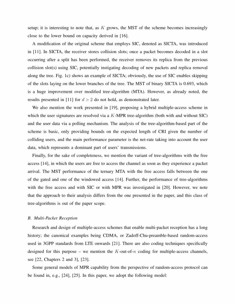
Fig. 1a) shows an example of the scheme. In practice, the CRP is combined with a channel-access

protocol (CAP), which specifies when the arriving (i.e., active) users can access the channel.

The basic variants of CAP are the gated (also known as blocked), windowed and free access; the

details about the former two are presented in Section V. It was shown that the MST throughput

of BTA with the gated access is 0.346 packet/slot [1].

This initial work inspired a number of research works on tree-algorithms. Here we mention the

modified tree-algorithm, which omits the slots that are certain to repeat the immediate previous

collision (e.g., slot 10 in Fig. 1a) would be skipped), boosting the MST with the gated access

to 0.375 packet/slot [15]. Another significant improvement can be obtained by using the BTA

in the windowed access framework, which boosts the MST to 0.429 packet/slot.

A further modification to the framework is made by considering d-ary splitting, a generalization

in which the colliding users split into d ≥ 2 groups. It was shown in [14] that the ternary tree-

algorithms with biased splitting (biased meaning that the probabilities of choosing a group are

not uniform over the groups) are the optimal choice. In this respect, a variant of the MTA

scheme with clipped access (a modification of the windowed access) introduced in [12] is the

best performing scheme in conventional setups (i.e., without MPR and SIC), achieving the MST

of 0.4878 packet/slot.

Supplementing tree-algorithms with K-MPR capability has the potential to improve their

3

5

2

2

1

1

1

1

2

3

4

5

6

7

2

0

8

13

0

2

9

10

a) c)

1

1

11

12

3

5

2

2

1

1

1

1

2

3

4

2

0

5

0

2

6

b)

1

1

7

3

5

2

2

1

1

2

3

4

5

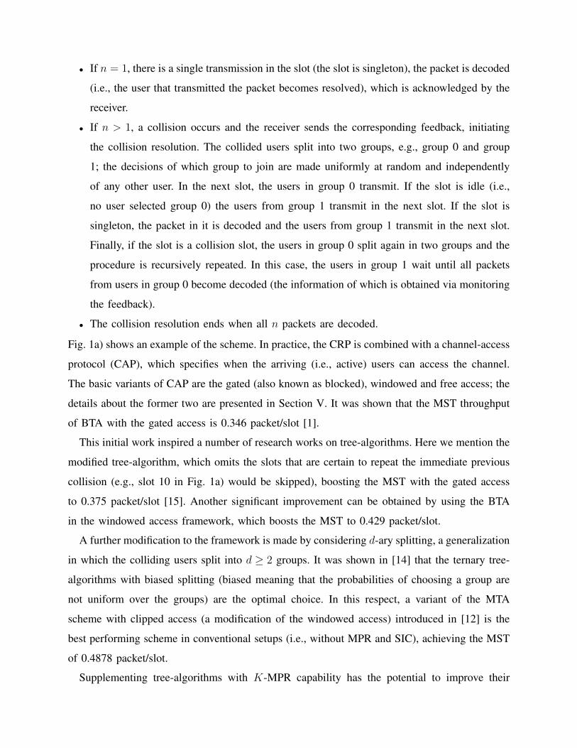
Fig. 1: Illustrative examples of binary tree-algorithms. A node of the tree represents a slot, the

number inside the node represents the number of users (i.e., packets) colliding in the slot, and the

number beneath represents the sequence number of the slot. a) BTA (the original version of the

algorithm): It is assumed that initially 5 users collided, which progressively split in two groups

until they become resolved (i.e., their packets decoded). b) BTA with 2 MPR: The receiver

is able to decode collisions of 2 or less packets, which reduces the number of slots required

to resolve all users. c) Binary tree-algorithm with SIC: The dashed nodes represent slots that

are skipped, as the users belonging to the corresponding groups are resolved by cancelling the

interference of the users resolved in the sibling node from the parent node, as indicated by the

grey arrows.

performance, as demonstrated in Fig. 1b). However, to the best of our knowledge, works studying

the impact of K-MPR capability on tree-algorithms are scarce. We mention the work deriving

an upper and lower bound on the MST (therein referred to as the capacity) for K-MPR tree

algorithm [16]. The work in [17] proposes a K-MPR tree algorithms with an adaptive form

of windowed access, where a part of the subsequent arrival window is added to the one being

currently resolved, depending on the outcomes of the collision resolution. The work in [18]

analyzes MPR in a tree-algorithm with continuous arrivals with a small number of users in the

system (of the order of 10), proposing a transmission strategy that guarantees stability. Finally,

the paper [13] performs the analysis of BTA with K-MPR in the standard windowed access

setup; it is interesting to note that, as K grows, the MST of the scheme becomes increasingly

close to the lower bound on capacity derived in [16].

A modification of the original scheme that employs SIC, denoted as SICTA, was introduced

in [11]. In SICTA, the receiver stores collision slots; once a packet becomes decoded in a slot

occurring after a split has been performed, the receiver removes its replica from the previous

collision slot(s) using SIC, potentially instigating decoding of new packets and replica removal

along the tree. Fig. 1c) shows an example of SICTA; obviously, the use of SIC enables skipping

of the slots laying on the lower branches of the tree. The MST of binary SICTA is 0.693, which

is a huge improvement over modified tree-algorithm (MTA). However, as already noted, the

results presented in [11] for d > 2 do not hold, as demonstrated later.

We also mention the work presented in [19], proposing a hybrid multiple-access scheme in

which the user signatures are resolved via a K-MPR tree-algorithm (both with and without SIC)

and the user data via a polling mechanism. The analysis of the tree-algorithm-based part of the

scheme is basic, only providing bounds on the expected length of CRI given the number of

colliding users, and the main performance parameter is the net-rate taking into account the user

data, which represents a dominant part of users’ transmissions.

Finally, for the sake of completeness, we mention the variant of tree-algorithms with the free

access [14], in which the users are free to access the channel as soon as they experience a packet

arrival. The MST performance of the ternary MTA with the free access falls between the one

of the gated and one of the windowed access [14]. Further, the performance of tree-algorithms

with the free access and with SIC or with MPR was investigated in [20]. However, we note

that the approach to their analysis differs from the one presented in the paper, and this class of

tree-algorithms is out of the paper scope.

B. Multi-Packet Reception

Research and design of multiple-access schemes that enable multi-packet reception has a long

history; the canonical examples being CDMA, or Zadoff-Chu-preamble-based random-access

used in 3GPP standards from LTE onwards [21]. There are also coding techniques specifically

designed for this purpose – we mention the K-out-of-n coding for multiple-access channels,

see [22, Chapters 2 and 3], [23].

Some general models of MPR capability from the perspective of random-access protocol can

be found in, e.g., [24], [25]. In this paper, we adopt the following model:

(i) if there are up to and including K packets colliding in a slot, all packets are successfully

decoded, and

(ii) if the number of colliding packets in a slot is greater than K, no packet can be successfully

decoded.

This model can be understood as an extension of the collision channel model (the default channel

model for the assessment of random-access algorithms). Specifically, it can be referred to as the

K-collision channel.

The works studying random-access protocols with MPR typically abstain from modelling the

investments required at the physical layer in order to enable the MPR. In this paper, we assume

that the K-MPR capability requires K times more (time-frequency) resources in comparison

to single-packet reception case (i.e., the required number of resources is directly proportional

to K). In effect, slots in K-collision channel are K times larger compared to the standard (1-

)collision channel, which is taken into account when assessing the performance, see Section III.

This model is adequate for CDMA [26] or some K-out-of-n coding schemes [19], [23], [27].

Finally, we remark that the assumed model is in a certain sense conservative. For instance, in

non-orthogonal multiple-access schemes which rely on power-imbalances among users’ trans-

missions, capture and successive interference cancellation, e.g., [28], [29], the increase in time-

frequency resources may not be needed. In this respect, the results presented in this paper can

be considered as a lower-bound on performance for the cases when K > 1.

III. SYSTEM MODEL

Consider n active users and a common access point (AP). The users are contending to access

the AP over a multiple-access K-collision channel with feedback by transmitting fixed-length

packets. The time-frequency resources of the channel are divided into slots dimensioned to

accommodate a single packet transmission. The users are synchronized on a slot basis via means

of the feedback sent by the AP. The feedback channel is broadcast and assumed perfect. The

feedback drives the contention process, as elaborated below.

The contention starts with all n users transmitting in the first slot that appears on the channel

and lasts until all users’ packets are successfully received. Henceforth, we also denote the event

of successful reception of a user packet as the user resolution.

We now elaborate in details the CRP according to which the collisions are resolved. Our focus

is on the binary tree-algorithms.3 Denote the slot number by j, with the initial value j = 1. The

number of users transmitting in slot j is denoted by nj . After every slot j, the AP transmits the

feedback signal fj , where

fj =

0, if nj = 0

s, if 0 < nj ≤ K

c, if nj > K

. (1)

In particular, fj = 0 denotes that j was an idle slot and fj = c that j was a collision slot.

When 0 < nj ≤ K, the packets transmitted in the slot were successfully decoded (i.e., the

slot was successful), triggering SIC upward along the tree. In this case, the feedback signal is

fj = s = j − p+ 1, where p denotes the last slot along the tree in which all users have become

resolved through the application of SIC, starting from the successful reception in slot j.

Every user i maintains a counter, whose state in slot j is denoted by Ci,j , with the initial

value Ci,1 = 0, ∀i. The state of the counter in slot j determines if the user will transmit in slot

j or not. Specifically, if Ci,j = 0, then user i transmits in slot j. If Ci,j > 0, user i abstains from

transmitting in slot j. Finally, if Ci,j becomes negative, i.e., Ci,j < 0, this indicates that user i

has become resolved and the user does not contend further. The state of the counter of user i is

updated reception of the feedback, as follows

Ci,j+1 =

bi,j, if fj = c and Ci,j = 0

Ci,j + 1, if fj = c and Ci,j > 0

Ci,j − s, if fj = s

bi,j, if fj = 0 and Ci,j = 1

Ci,j + 1, if fj = 0 and Ci,j > 1

(2)

where bi,j is a Bernoulli random variable that takes value 0 with probability p and value 1 with

probability 1− p; if p = 1/2, the splitting is fair. The topmost case in (2) corresponds to a split

that occurs after the contention in slot j, in which user i took part, resulted in a collision. If

bi,j = 0 user i joins the generic group 0, and if bi,j = 1 the user joins group 1. The second

case in (2) corresponds to a scenario in which user i did not transmit in slot j, the slot resulted

3Some insights on d-ary tree-algorithms with SIC, for d > 2 are provided in Section VI.

3

5

2

0

3

1

2

3 2

1

4

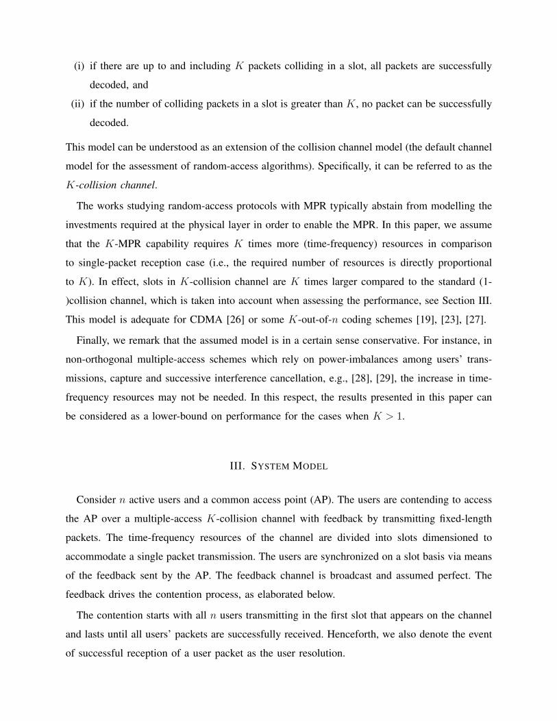
Fig. 2: Example of binary tree-algorithm with SIC (SICTA) on 2-Collision Channel with SIC.

in the collision, and the user increases its counter to reflect the fact that the ongoing collision

resolution will last an additional slot. In the third case, the slot was successful, the SIC process

was triggered, and the counter is decreased for the number of slots in which the users were

resolved in this round. The fourth and the fifth (i.e. the last case) in (2) refers to the scenario in

which an idle slot occurred, and the users in the parent slot perform an immediate split, while

the other unresolved users increment their counters.4.

To facilitate a better understanding, the example in Fig. 2 illustrates the contention on 2-

collision channel with SIC, and Table I lists the corresponding states of the users’ counters. It

is assumed in the example that: (i) after slot 1, user 1, user 3 and user 4 chose group 0, while

user 2 and user 5 chose group 1; (ii) after slot 2, no user chose group 0, and user 1, user 3 and

user 4 chose group 1; and (iii) after slot 3, user 1 and user 4 chose group 0, while user 3 chose

group 1.

The period elapsed from the first slot up to and including the last slot in which all n users

become resolved is denoted as CRI. The length of CRI in slots conditioned on n is a random

variable denoted by ln. The basic performance parameter of interest is the expected value of ln,

denoted by Ln, i.e., Ln = E[ln]. Another important performance parameter is the conditional

4We note that a similar protocol for updating the state of the users’ counters was presented in [11]. Among others, a major

difference is that the feedback in the case of successful slot in [11] provides a sum of the number of resolved users and idle

slots.

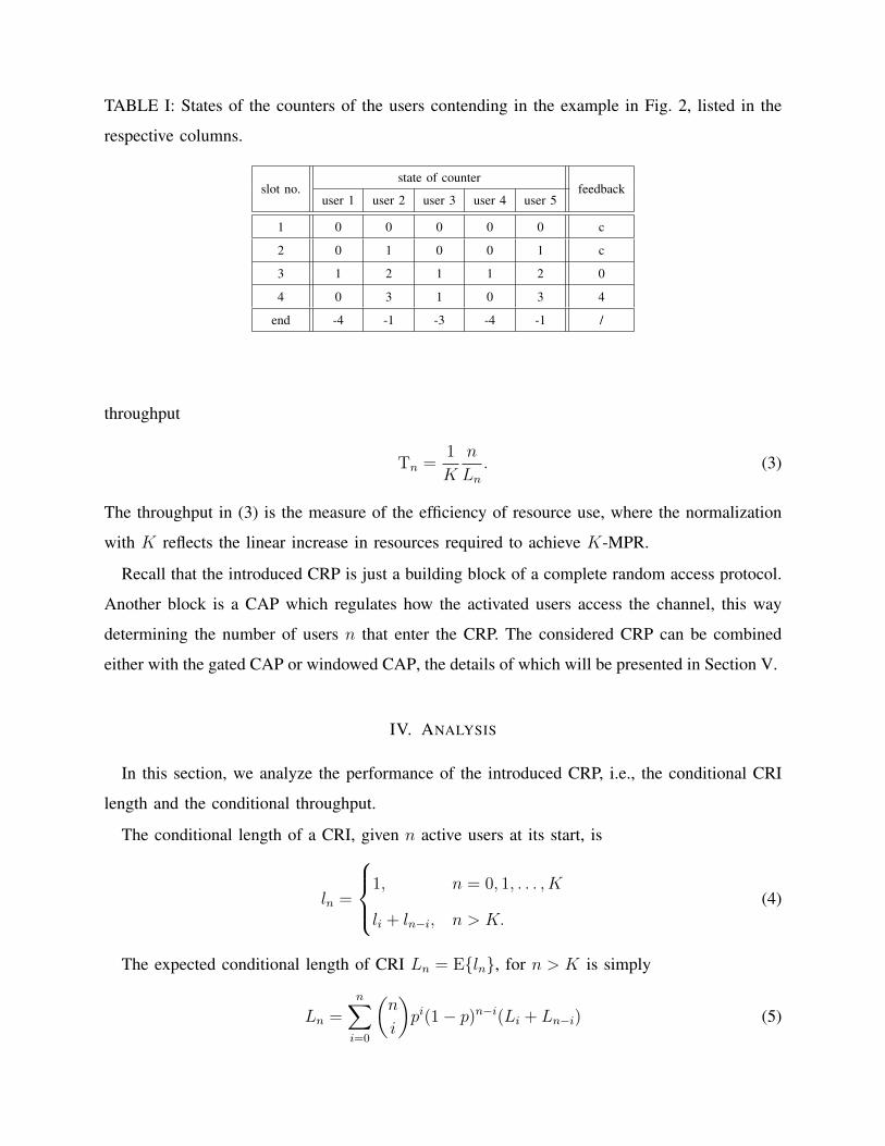
TABLE I: States of the counters of the users contending in the example in Fig. 2, listed in the

respective columns.

slot no.state of counter

feedbackuser 1 user 2 user 3 user 4 user 5

1 0 0 0 0 0 c

2 0 1 0 0 1 c

3 1 2 1 1 2 0

4 0 3 1 0 3 4

end -4 -1 -3 -4 -1 /

throughput

Tn =1

K

n

Ln. (3)

The throughput in (3) is the measure of the efficiency of resource use, where the normalization

with K reflects the linear increase in resources required to achieve K-MPR.

Recall that the introduced CRP is just a building block of a complete random access protocol.

Another block is a CAP which regulates how the activated users access the channel, this way

determining the number of users n that enter the CRP. The considered CRP can be combined

either with the gated CAP or windowed CAP, the details of which will be presented in Section V.

IV. ANALYSIS

In this section, we analyze the performance of the introduced CRP, i.e., the conditional CRI

length and the conditional throughput.

The conditional length of a CRI, given n active users at its start, is

ln =

1, n = 0, 1, . . . , K

li + ln−i, n > K.(4)

The expected conditional length of CRI Ln = E{ln}, for n > K is simply

Ln =n∑i=0

(n

i

)pi(1− p)n−i(Li + Ln−i) (5)

where p is the probability of a user joining the first group. By developing (5), Ln can be calculated

recursively through

Ln =

1, n ≤ K

pn+(1−p)n+2∑n−1

i=1 (ni)pn−i(1−p)iLi

1−pn−(1−p)n , n > K.(6)

A. Direct Expression for Ln

For the derivation of the direct, i.e. non-recursive expression for Ln, we rely on the method

that relies on generating functions, elaborated in [14]. We start by introducing the conditional

probability generating function (CPGF) of ln is given by

Qn(z) = E{zln}

(7)

where, due to (4), the following holds

Q0(z) = Q1(z) = · · · = QK(z) = z. (8)

For n > K, we have

Qn(z) =n∑i=0

(n

i

)pi(1− p)n−iQi(z)Qn−i(z). (9)

The (unconditional) probability generating function (PGF) of CRI, assuming that n obeys a

Poisson distribution5 with a mean x, is given by

Q(x, z) =∞∑n=0

Qn(z)xn

n!e−x (10)

=∞∑n=0

xn

n!e−x

n∑i=0

(n

i

)pi(1− p)n−iQi(z)Qn−i(z)+

+(z − z2

) K∑k=0

xk

k!e−x (11)

where we exploited (8), (9), and the fact that for n ≤ Kn∑i=0

(n

i

)pn−i(1− p)iQn−i(z)Qi(z) = z2. (12)

The first term on right-hand side (rhs) in (11) can be transformed into∞∑n=0

Qn(z)(px)n

n!e−px

∞∑i=0

Qi(z)((1− p)x)i

i!e−(1−p)x (13)

5This is an auxiliary assumption that will not limit the general nature of the derived results.

so that (11) becomes

Q(x, z) = Q(px, z)Q ((1− p)x, z) +(z − z2

) K∑k=0

xk

k!e−x. (14)

Further, using the fact that dQn(z)dz|z=1 = Ln, from (10) we get

∂Q(x, z)

∂z

∣∣∣z=1

= L(x) =∞∑n=0

Lnxn

n!e−x. (15)

L(x) is also known as transformed generating function (TGF) of Ln. Taking the partial derivative

of (14) with respect to z at z = 1 yields

L(x) = L(px) + L((1− p)x)−K∑k=0

xk

k!e−x (16)

where we used the fact that Q(x, 1) = 1, ∀x.

In the next step, we assume the following power series representation of L(x)

L(x) =∞∑n=0

αnxn (17)

where it can be shown that

Ln =n∑j=0

n!

(n− j)!αj. (18)

We now compute αj , j = 0, 1, . . . , n. From (6), it follows that

αj =

1, j = 0

0, j = 1, . . . , K.(19)

Substituting (17) into (16) and using Maclaurin series expansion for e−x yields

∞∑n=0

αn(1− pn − (1− p)n)xn =−K∑k=0

xk

k!

∞∑n=0

(−1)nxn

n!

=∞∑n=0

min(n,K)∑k=0

(−1)n−k+1

k!(n− k)!xn. (20)

For n ≤ K, it can be shown that

n∑k=0

(−1)n−k+1

k!(n− k)!=

−1, n = 0

0, 0 < n ≤ K(21)

100

101

102

103

n

100

101

102

103

KL

n

K=1K=2K=4K=8K=16

Fig. 3: K · Ln as function of n for K ∈ {1, 2, 4, 8, 16, 32}.

which, coupled with (19), transforms (20) into

∞∑n=K+1

αn(1− pn−(1− p)n)xn =

=∞∑

n=K+1

K∑k=0

(−1)n−k+1

k!(n− k)!xn. (22)

Solving (22) for αn, n ≥ K, we get

αn =K∑k=0

(−1)n−k+1

k!(n− k)!· 1

1− pn − (1− p)n. (23)

By substituting (19) and (23) in (18) for n > K, and after some manipulation, we get

Ln = 1 +n∑

j=K+1

(n

j

)(−1)j+1

1− pj − (1− p)jK∑k=0

(j

k

)(−1)−k. (24)

Using the identity that holds for K < j

K∑k=0

(−1)k(j

k

)= (−1)K

(j − 1

K

)(25)

100

101

102

103

n

0.55

0.6

0.6536

0.6931

0.7378

0.8

0.85

0.9

0.95

Tn

K=1K=2K=4K=8K=16K=32

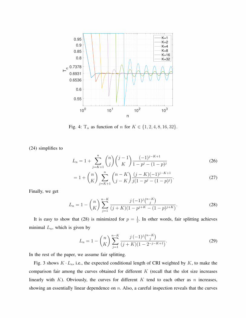
Fig. 4: Tn as function of n for K ∈ {1, 2, 4, 8, 16, 32}.

(24) simplifies to

Ln = 1 +n∑

j=K+1

(n

j

)(j − 1

K

)(−1)j−K+1

1− pj − (1− p)j(26)

= 1 +

(n

K

) n∑j=K+1

(n−Kj −K

)(j −K)(−1)j−K+1

j(1− pj − (1− p)j). (27)

Finally, we get

Ln = 1−(n

K

) n−K∑j=1

j (−1)j(n−Kj

)(j +K)(1− pj+K − (1− p)j+K)

. (28)

It is easy to show that (28) is minimized for p = 12. In other words, fair splitting achieves

minimal Ln, which is given by

Ln = 1−(n

K

) n−K∑j=1

j (−1)j(n−Kj

)(j +K)(1− 2−j−K+1)

. (29)

In the rest of the paper, we assume fair splitting.

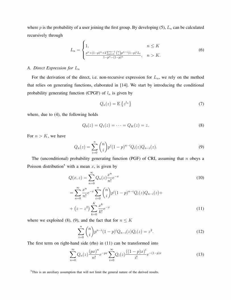
Fig. 3 shows K ·Ln, i.e., the expected conditional length of CRI weighted by K, to make the

comparison fair among the curves obtained for different K (recall that the slot size increases

linearly with K). Obviously, the curves for different K tend to each other as n increases,

showing an essentially linear dependence on n. Also, a careful inspection reveals that the curves

show an oscillatory behaviour, with the oscillations periodicity depending on log(n) and the

oscillations amplitude increasing with K. This oscillatory behaviour is more evident in Fig. 4,

which shows the conditional throughput Tn as function of n. The oscillations are non-vanishing,

a fact identified in [14] for the binary tree-algorithms on the standard collision channel. We

analytically investigate this phenomenon in the next subsection.

More importantly, both Fig. 3 and Fig. 4 suggest that the use of MPR does not improve the

performance of the tree-algorithm conditioned on n, when normalized with K. In particular,

Fig. 4 shows that, as n→∞, Tn oscillates around the value of ln(2) ≈ 0.6931, irrespective of

the value of K. In Section V, we make further investigations of this issue.

B. Asymptotic behaviour of Ln

Here we turn to analysis of asymptotic behavior of Ln, exploiting the approach presented in

[14]. Rewriting (16) for the case of fair-splitting (i.e., p = 1/2), we get

L(x)− 2L(x

2

)= −

K∑k=0

xk

k!e−x. (30)

By differentiating (30) twice, we get

L′′(x)− 1

2L′′(x

2

)=

[xK−1

(K − 1)!− xK

K!

]e−x = g(x) (31)

which is a functional equation that satisfies the contraction condition and has the solution in the

form [14]

L′′(x) =∞∑m=0

1

2mg( x

2m

)(32)

=∞∑m=0

1

2m

[(x

2m

)K−1

(K − 1)!−(x

2m

)KK!

]e−

x2m . (33)

Integrating (32) twice, and taking into account the initial conditions L(0) = 1 and L′(0) = 0

that stem from (15), we obtain the following expression for the TGF

L(x) = 1 +∞∑m=0

2m −∞∑m=0

2me−x

2m

K∑k=0

(x

2m

)kk!

(34)

Exploiting (15) further, the previous equation can be transformed to

∞∑n=0

Lnxn

n!= ex + ex

∞∑m=0

2m

[1− e−

x2m

K∑k=0

(x

2m

)kk!

]. (35)

Using the Maclaurin series expansion for ex, and after some manipulation, we transform (35)

into

∞∑n=0

Lnxn

n!=∞∑n=0

xn

n!×1 +

∞∑m=0

2m

1−min{n,K}∑

k=0

(n

k

)(1− 1

2m)n−k

2mk

. (36)

Equating coefficients for xn, n > K, we get

Ln = 1 +∞∑m=0

2m

[1−

K∑k=0

(n

k

)(1− 1

2m

)n−k2mk

]. (37)

In principle, from (37) one can derive the same expression for Ln given by (29). However, we do

not pursue this further. Instead, assuming that K is fixed, we exploit the following approximations

for n� K (1− 1

2m

)n−k= e−

n2m

(1− kn

)+( n2m )

2O(n−1) ≈ e−

n2m (38)(

n

k

)=nk

k!

(1− k(k − 1)

2Θ(n−1)

)≈ nk

k!(39)

which, substituted into (37), yield

Ln ≈ 1 +∞∑m=0

2m

[1−

K∑k=0

( n2m

)k e− n2m

k!

]. (40)

Now, the task at hand is to isolate n in (40), such that summation over m can be performed. For

this purpose, we exploit the method for the asymptotic analysis of harmonic sums [14], [30].

We introduce the following function

g(x) = 1−K∑k=0

xk

k!e−x. (41)

The Mellin transform of g(x) is

G(s) =

∫ ∞0

g(x)xs−1dx = −Γ(s)

[1 +

K∑k=1

∏k−1i=0 (s+ i)

k!

]

= −(s+ 1)Γ(s)

[1 +

s

2!+ s

K∑k=3

∏k−1i=2 (s+ i)

k!

](42)

where s is a complex variable laying in the fundamental strip (i.e., strip of convergence) given

by −2 < Re(s) < 0 and Γ(s) is the meromorphic extension of the Gamma function. The inverse

Mellin transform for x = n/2m is given by

g( n

2m

)=

1

2πj

∫ η+j∞

η−j∞G(s)

( n2m

)−sds = (43)

− 1

2πj

∫ η+j∞

η−j∞Γ(s)

[1 +

K∑k=1

∏k−1i=0 (s+ i)

k!

]n−s

2−msds

where η belongs to the fundamental strip. Substituting (43) into (40), and interchanging the order

of summation and integration, we obtain

Ln ≈ 1 +1

2πj

∫ η+j∞

η−j∞G(s)n−s

∞∑m=0

2(s+1)m (44)

= 1 +1

2πj

∫ η+j∞

η−j∞

G(s)n−s

1− 2s+1ds. (45)

The domain of absolute convergence of the series in (44) is Re(s) < −1. Thus, the fundamental

strip of the integrand

H(s) =G(s)n−s

1− 2s+1(46)

lies in the intersection of the domain of absolute convergence of the series and the fundamental

strip of G(s), and is given by −2 < <(s) < −1. In this strip lies η in (45).

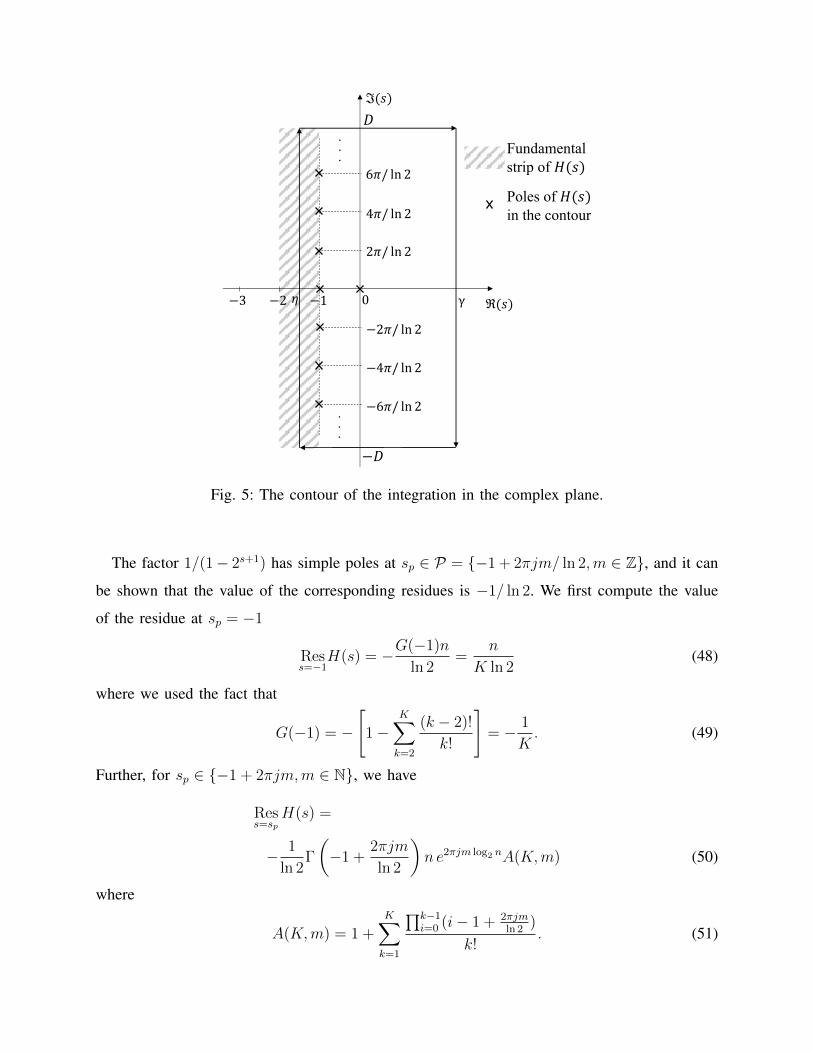
We compute the integral in (45) using the residue theorem. In order to evaluate Ln for n→∞,

we close the path of integration in the half of the complex plane that is right to the fundamental

strip, see Fig. 5. The gamma function decays exponentially fast as the absolute value of the

imaginary component of the argument increases, thus, the integration on the horizontal parts of

the contour tends to zero as |D| → ∞. The integral on the vertical line <(s) = γ, γ > 0, is

bounded by O(n−γ), also tending to zero for large n [31, Chapter 5.2.2], [30]. Thus, the integral

in (45) is equal to the negative sum of the residues of the poles of H(s) within the contour

(negative due to the contour orientation).

The factor n−s trivially has no poles in the contour. Further, g(s) has a simple pole in 0 which

is due to the corresponding pole of Γ(s).6 We have

Ress=0

H(s) = −Γ(0) = −1. (47)

6For the sake of completeness, we note that the pole of Γ(s) at −1 is cancelled out by the zero (s+ 1) of the function G(s),

see (42).

ℜ(𝑠)

ℑ(𝑠)

−1−2 0−3 γ𝜂

−2𝜋/ ln 2

−4𝜋/ ln 2

2𝜋/ ln 2

4𝜋/ ln 2

. .

.

6𝜋/ ln 2

−6𝜋/ ln 2

. .

.

Fundamental strip of 𝐻(𝑠)

Poles of 𝐻(𝑠)in the contour

𝐷

−𝐷

Fig. 5: The contour of the integration in the complex plane.

The factor 1/(1− 2s+1) has simple poles at sp ∈ P = {−1 + 2πjm/ ln 2,m ∈ Z}, and it can

be shown that the value of the corresponding residues is −1/ ln 2. We first compute the value

of the residue at sp = −1

Ress=−1

H(s) = −G(−1)n

ln 2=

n

K ln 2(48)

where we used the fact that

G(−1) = −

[1−

K∑k=2

(k − 2)!

k!

]= − 1

K. (49)

Further, for sp ∈ {−1 + 2πjm,m ∈ N}, we have

Ress=sp

H(s) =

− 1

ln 2Γ

(−1 +

2πjm

ln 2

)n e2πjm log2 nA(K,m) (50)

where

A(K,m) = 1 +K∑k=1

∏k−1i=0 (i− 1 + 2πjm

ln 2)

k!. (51)

Similarly, for sp ∈ {−1− 2πjm,m ∈ N} we have

Ress=sp

H(s) = (52)

− 1

ln 2Γ

(−1− 2πjm

ln 2

)n e−2πjm log2 nA(K,−m). (53)

Using the mirror-symmetry property that holds for the gamma function

Γ(s∗) = Γ∗(s) (54)

where ∗ denotes the complex conjugate, and using the following identity (which can be trivially

shown)

A(K,−m) = A∗(K,m) (55)

we get ∑sp∈P\{0}}

Ress=sp

H(s) = − 2n

ln 2

∞∑m=1

<(B(K,m)e2πjm log2 n

)= − 2n

ln 2

∞∑m=1

|B(K,m)| cos (2πm log2 n+ arg (B(K,m))) (56)

where

B(K,m) = Γ

(−1 +

2πjm

ln 2

)A(K,m). (57)

Again, since the gamma function decays exponentially fast as the imaginary component of the

argument increases, (56) can be approximated as∑sp∈P\{0}}

ResH(s)s=sp

≈ (58)

− 2n

ln 2|B(K, 1)| cos (2π log2 n+ arg (B(K, 1))) .

Putting all the pieces together, we obtain for the expected conditional length of CRI, when

n→∞, to be

Ln ≈n

K ln 2×

(1− 2K|B(K, 1)|) cos(2π log2 n+ arg(B(K, 1))). (59)

The conditional throughput, when n→∞, is

Tn =n

KLn

≈ ln 2

1− 2K|B(K, 1)| cos(2π log2 n+ arg(B(K, 1))). (60)

0 20 40 60 80 100

K

10-6

10-4

10-2

100

2K

|B

(K,1

)|

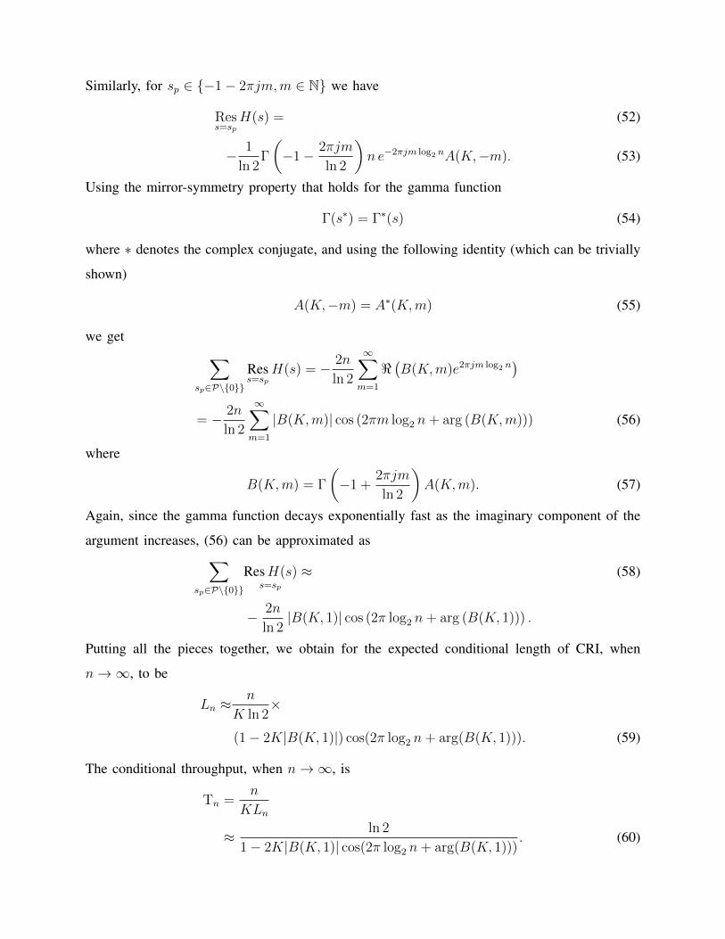
Fig. 6: The amplitude of the oscillatory component in (59) and (60), as function of K.

This oscillatory component in log2 n was identified in, e.g., [14], [30], [32]. In the case treated

here, the difference is that its amplitude depends on K and can not be neglected, as it affects

the stability bound (further discussed in Section V).

The expression 2K|B(K, 1)| can be easily computed for any K. The graph presented in Fig. 6

shows that its value increases with K, which is also confirmed in Fig. 3 and Fig. 4. Although of

a little practical relevance, an interesting problem in its own right is to determine the behaviour

of K|B(K, 1)| as K → ∞. This problem is out of the paper scope; based on our preliminary

investigation, we conjecture that that there is an upper bound on the value of K|B(K, 1)| as

K →∞.

Finally, we validate the presented analysis by comparing its output with the results presented in

Fig. 4. For instance, 2K|B(K, 1)| evaluates to 0.0607 for K = 32, implying that the asymptotic

maximum and minimum values of Tn are 0.7378 and 0.6536, respectively, see (60). Obviously,

the curve for Tn when K = 32 in Fig. 4 indeed tends to oscillate between these two values as

n increases.

C. Simple bounds on Ln and Tn

We conclude this section by developing simple, but useful bounds on Ln and Tn, that do not

require asymptotic evaluation presented. In particular, these bounds can be computed for any

TABLE II: Bounds on expected conditional length of CRI and conditional throughput.

K m n αm βm Am Bm

1 50 100 1.4427 1.4427 0.6931 0.6931

2 100 200 0.7214 0.7213 0.6931 0.6932

4 200 400 0.3607 0.3606 0.6930 0.6933

8 400 800 0.1808 0.1799 0.6915 0.6948

16 400 800 0.0919 0.0884 0.6803 0.7069

32 400 800 0.0480 0.0421 0.6505 0.7420

64 500 1000 0.0254 0.0199 0.6141 0.7864

finite m and are valid for any n ≥ m.

For n > K and fair splitting, the expected conditional length of CRI reduces to

Ln =

∑n−1i=0

(ni

)Li

2n−1 − 1. (61)

Following the method introduced by Massey [15], we want to find the constant αm for which

the following holds:

Ln ≤ αmn, n ≥ m. (62)

For n < m, we can write

Ln ≤ αmn+M−1∑i=1

δi,n(Ln − αmn) (63)

where δi,n is the Kronecker delta, and where (63) holds by definition. In the induction step, we

substitute (63) into (61), and after some manipulation, obtain

Ln ≤ αmn+

∑m−1i=0

(ni

)(Li − αmi)

2n−1 − 1(64)

and the condition (62) will hold true for any

αm ≥∑m−1

i=0

(ni

)Li∑m−1

i=0

(ni

)i

(65)

as the summation in the second term on the right-hand side of (64) is non-positive in this case.

The tightest upper bound is given by

αm = supn≥m

∑m−1i=0

(ni

)Li∑m−1

i=0

(ni

)i. (66)

arrivals

CRI 𝑖 − 1 CRI 𝑖 CRI 𝑖 + 1… …

𝑙!"#$ 𝑙!" 𝑙!"%$

𝑡

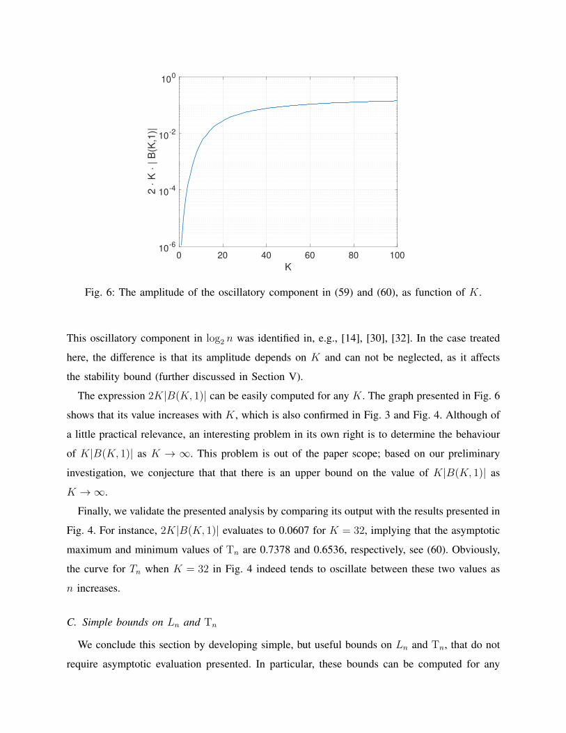
Fig. 7: Illustration of the gated access: users arriving during i-th CRI are resolved in (i+ 1)-th

CRI.

In a completely analogous fashion, one can find the lower bound

Ln ≥ βmn, n ≥ m (67)

where

βm = infn≥m

∑m−1i=0

(ni

)Li∑m−1

i=0

(ni

)i. (68)

Note that the bounds in (66) and (68) can be made arbitrarily tight by increasing m and n.

The corresponding bounds on conditional throughput are simply

Bm =1

Kβm≥ Tn ≥

1

Kαm= Am, n ≥ m. (69)

In Table II, we list αm, βm, Am and Bm (rounded up to four decimal places). Note the

agreement between the bounds on Tn shown in the table, i.e., Am and Bm, and the results

plotted in Fig. 4.

V. PERFORMANCE UNDER POISSON ARRIVALS

In this section, we provide insights into performance of a random access protocol that combines

the CRP protocol introduced in Section III with the gated CAP and the windowed CAP. We

adopt the standard performance evaluation approach by assuming Poisson arrivals in an infinite

user population; the arrival intensity per slot is denoted by λ. We are interested to identify the

bounds on λ for which the random access protocol features a stable operation. In brief, the

stability implies that the individual packets are successfully received with a finite delay almost

surely [14].

A. Gated Access

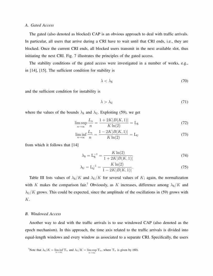
The gated (also denoted as blocked) CAP is an obvious approach to deal with traffic arrivals.

In particular, all users that arrive during a CRI have to wait until that CRI ends, i.e., they are

blocked. Once the current CRI ends, all blocked users transmit in the next available slot, thus

initiating the next CRI. Fig. 7 illustrates the principles of the gated access.

The stability conditions of the gated access were investigated in a number of works, e.g.,

in [14], [15]. The sufficient condition for stability is

λ < λS (70)

and the sufficient condition for instability is

λ > λU (71)

where the values of the bounds λS and λU. Exploiting (59), we get

lim supn→∞

Lnn

=1 + 2K|B(K, 1)|

K ln(2)= LS (72)

lim infn→∞

Lnn

=1− 2K|B(K, 1)|

K ln(2)= LU (73)

from which it follows that [14]

λS = L−1S =

K ln(2)

1 + 2K|B(K, 1)|(74)

λU = L−1U =

K ln(2)

1− 2K|B(K, 1)|. (75)

Table III lists values of λS/K and λU/K for several values of K; again, the normalization

with K makes the comparison fair.7 Obviously, as K increases, difference among λS/K and

λU/K grows. This could be expected, since the amplitude of the oscillations in (59) grows with

K.

B. Windowed Access

Another way to deal with the traffic arrivals is to use windowed CAP (also denoted as the

epoch mechanism). In this approach, the time axis related to the traffic arrivals is divided into

equal-length windows and every window as associated to a separate CRI. Specifically, the users

7Note that λS/K = lim infn→∞

Tn and λU/K = lim supn→∞

Tn, where Tn is given by (60).

TABLE III: Stability bounds on normalized traffic arrival intensity for gated access.

K λS/K λU/K

1 0.6931 0.6931

2 0.6931 0.6932

4 0.6930 0.6932

8 0.6916 0.6947

16 0.6811 0.7056

32 0.6536 0.7378

64 0.6216 0.7833

arriving in i-the window transmit in the first slot after the CRI of the users arriving in (i− 1)-th

window ends, thus starting their own CRI. Fig. 8 illustrates the windowed access.

Denoting the window length in slots by ∆ (which does not have to be an integer), the

probability of n arrivals (n ∈ N) in the window can be calculated as

Pr{N = n} =λ∆

n!e−λ∆, (76)

i.e., n is a Poisson random variable (r.v.) with mean λ∆. The expected length of CRI is

L(λ∆) = E{Ln|λ∆} =∞∑n=0

Ln(λ∆)n

n!e−λ∆. (77)

The necessary condition for stability is the following

L(λ∆) < ∆ (78)

which is intuitively clear, as it ensures that arrivals in a window will be served (on average) in

CRI that will last shorter than the window.8

Exploiting the bounds derived in Section IV-C, it is easy to show that

f(αm,m, λ∆) ≤ L(λ∆) ≤ f(βm,m, λ∆) (79)

where

f(x, k, z) = x · z +k∑i=0

(Li − x · i)zi

i!e−z. (80)

8For stability to hold, the condition E{L2n} <∞ has also to be satisfied. This can be shown for L(λ∆) < ∆, however, we

omit the proof.

arrivals𝑡window 𝑖 − 1 window 𝑖 window 𝑖 + 1 ……

CRI 𝑖 − 1 CRI 𝑖 CRI 𝑖 + 1… …

Δ Δ Δ

𝑙!"#$ 𝑙!" 𝑙!"%$

𝑡

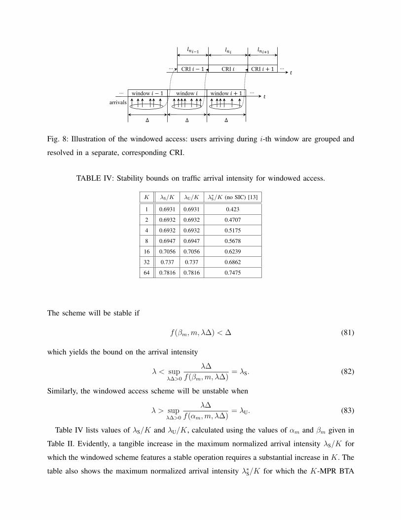
Fig. 8: Illustration of the windowed access: users arriving during i-th window are grouped and

resolved in a separate, corresponding CRI.

TABLE IV: Stability bounds on traffic arrival intensity for windowed access.

K λS/K λU/K λ∗S/K (no SIC) [13]

1 0.6931 0.6931 0.423

2 0.6932 0.6932 0.4707

4 0.6932 0.6932 0.5175

8 0.6947 0.6947 0.5678

16 0.7056 0.7056 0.6239

32 0.737 0.737 0.6862

64 0.7816 0.7816 0.7475

The scheme will be stable if

f(βm,m, λ∆) < ∆ (81)

which yields the bound on the arrival intensity

λ < supλ∆>0

λ∆

f(βm,m, λ∆)= λS. (82)

Similarly, the windowed access scheme will be unstable when

λ > supλ∆>0

λ∆

f(αm,m, λ∆)= λU. (83)

Table IV lists values of λS/K and λU/K, calculated using the values of αm and βm given in

Table II. Evidently, a tangible increase in the maximum normalized arrival intensity λS/K for

which the windowed scheme features a stable operation requires a substantial increase in K. The

table also shows the maximum normalized arrival intensity λ∗S/K for which the K-MPR BTA

0 50 100 150 2000

0.1

0.2

0.3

0.4

0.5

0.6

0.7

0.8

F(

)

K=1K=16K=64K=1, no SICK=16, no SICK=64, no SIC

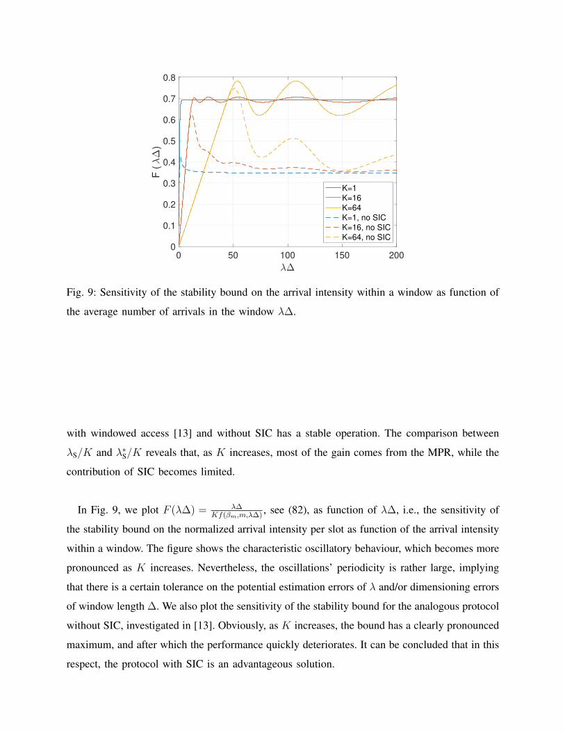
Fig. 9: Sensitivity of the stability bound on the arrival intensity within a window as function of

the average number of arrivals in the window λ∆.

with windowed access [13] and without SIC has a stable operation. The comparison between

λS/K and λ∗S/K reveals that, as K increases, most of the gain comes from the MPR, while the

contribution of SIC becomes limited.

In Fig. 9, we plot F (λ∆) = λ∆Kf(βm,m,λ∆)

, see (82), as function of λ∆, i.e., the sensitivity of

the stability bound on the normalized arrival intensity per slot as function of the arrival intensity

within a window. The figure shows the characteristic oscillatory behaviour, which becomes more

pronounced as K increases. Nevertheless, the oscillations’ periodicity is rather large, implying

that there is a certain tolerance on the potential estimation errors of λ and/or dimensioning errors

of window length ∆. We also plot the sensitivity of the stability bound for the analogous protocol

without SIC, investigated in [13]. Obviously, as K increases, the bound has a clearly pronounced

maximum, and after which the performance quickly deteriorates. It can be concluded that in this

respect, the protocol with SIC is an advantageous solution.

VI. REMARKS ON d-ARY TREE ALGORITHMS WITH SIC

As discussed in Section II-A, d-ary tree algorithms (i.e., tree-algorithms in which the number of

groups in which users can split is generalized to d)9, show benefits in the original scenario (i.e.,

without SIC and MPR). In particular, it was shown that the ternary version of the algorithm

(i.e., when d = 3) with optimized splitting probabilities outperforms the binary version. A

natural question is whether analogous results can be established for the variant of tree algorithms

examined in this paper.

In this respect, the analysis presented in [11, Section IV-A] is performed for d-ary tree

algorithms with SIC when K = 1. However, the initial premise of the analysis is incorrect

when d > 2. The premise states the following (verbatim):

ln =

1, if n = 0, 1∑dj=i lIj , if n ≥ 2

(84)

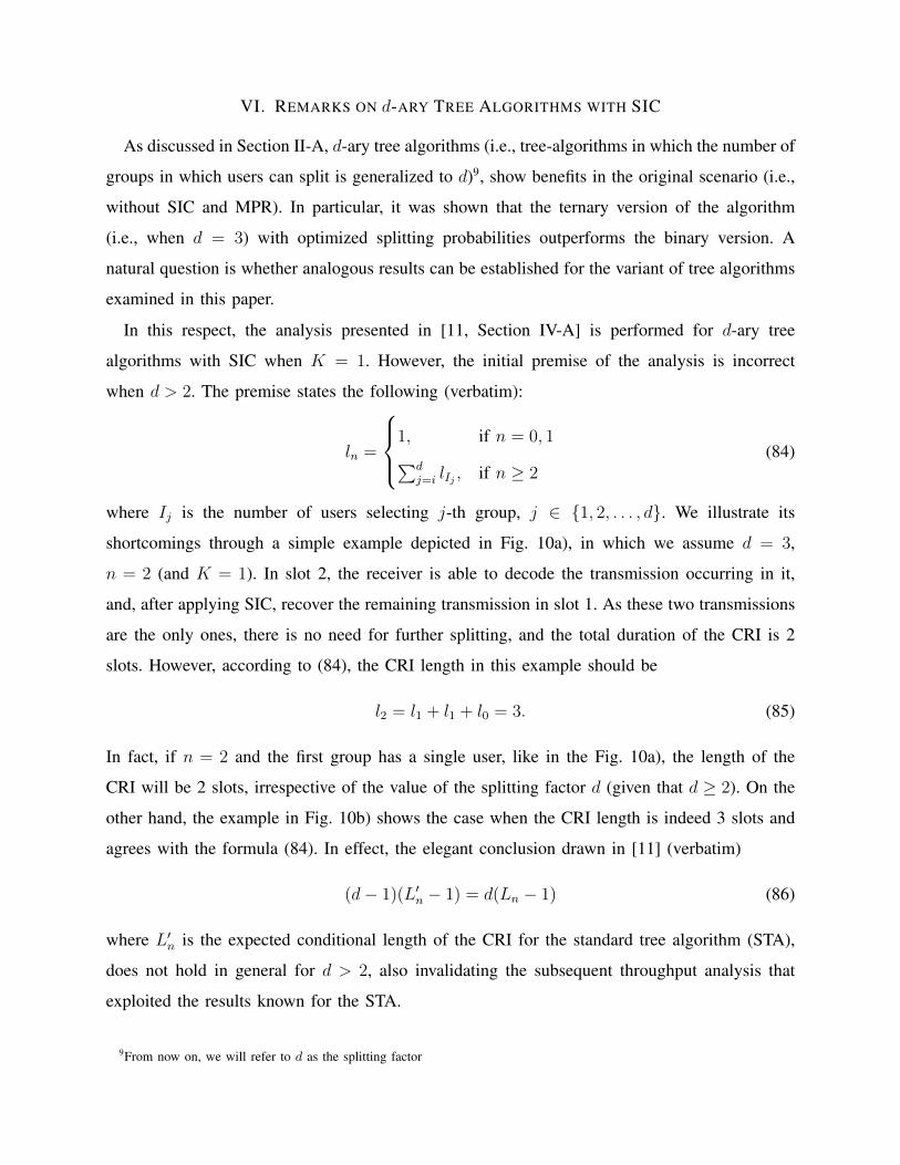
where Ij is the number of users selecting j-th group, j ∈ {1, 2, . . . , d}. We illustrate its

shortcomings through a simple example depicted in Fig. 10a), in which we assume d = 3,

n = 2 (and K = 1). In slot 2, the receiver is able to decode the transmission occurring in it,

and, after applying SIC, recover the remaining transmission in slot 1. As these two transmissions

are the only ones, there is no need for further splitting, and the total duration of the CRI is 2

slots. However, according to (84), the CRI length in this example should be

l2 = l1 + l1 + l0 = 3. (85)

In fact, if n = 2 and the first group has a single user, like in the Fig. 10a), the length of the

CRI will be 2 slots, irrespective of the value of the splitting factor d (given that d ≥ 2). On the

other hand, the example in Fig. 10b) shows the case when the CRI length is indeed 3 slots and

agrees with the formula (84). In effect, the elegant conclusion drawn in [11] (verbatim)

(d− 1)(L′n − 1) = d(Ln − 1) (86)

where L′n is the expected conditional length of the CRI for the standard tree algorithm (STA),

does not hold in general for d > 2, also invalidating the subsequent throughput analysis that

exploited the results known for the STA.

9From now on, we will refer to d as the splitting factor

1

2

0

1

2

1

a) 0

2

1

1

2

1

b)

3

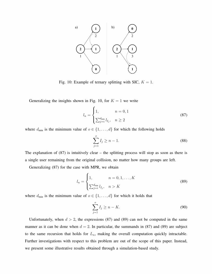
Fig. 10: Example of ternary splitting with SIC, K = 1.

Generalizing the insights shown in Fig. 10, for K = 1 we write

ln =

1, n = 0, 1∑dminj=i lIj , n ≥ 2

(87)

where dmin is the minimum value of o ∈ {1, . . . , d} for which the following holdso∑j=1

Ij ≥ n− 1. (88)

The explanation of (87) is intuitively clear – the splitting process will stop as soon as there is

a single user remaining from the original collision, no matter how many groups are left.

Generalizing (87) for the case with MPR, we obtain

ln =

1, n = 0, 1, . . . , K∑dminj=i lIj , n > K

(89)

where dmin is the minimum value of o ∈ {1, . . . , d} for which it holds thato∑j=1

Ij ≥ n−K. (90)

Unfortunately, when d > 2, the expressions (87) and (89) can not be computed in the same

manner as it can be done when d = 2. In particular, the summands in (87) and (89) are subject

to the same recursion that holds for Ln, making the overall computation quickly intractable.

Further investigations with respect to this problem are out of the scope of this paper. Instead,

we present some illustrative results obtained through a simulation-based study.

2 3 4 5 6 7 8 9

d

0.2

0.3

0.4

0.5

0.6

0.7MST from [12]

Tn, n = 1000

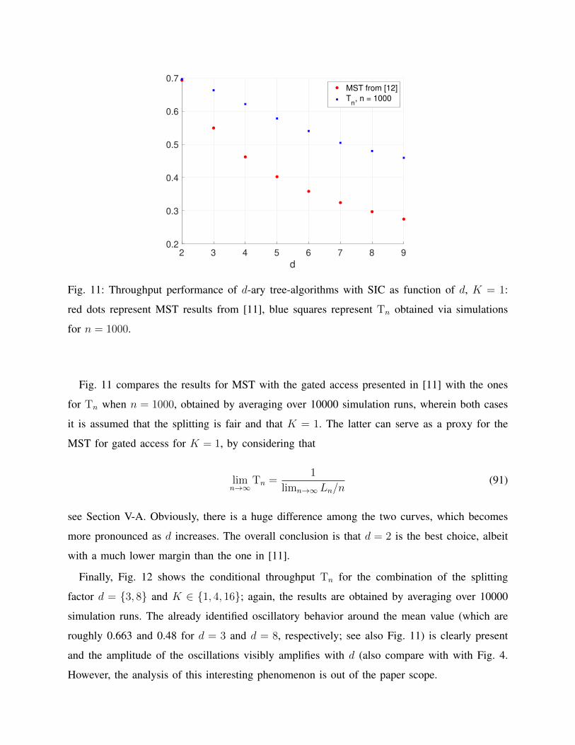
Fig. 11: Throughput performance of d-ary tree-algorithms with SIC as function of d, K = 1:

red dots represent MST results from [11], blue squares represent Tn obtained via simulations

for n = 1000.

Fig. 11 compares the results for MST with the gated access presented in [11] with the ones

for Tn when n = 1000, obtained by averaging over 10000 simulation runs, wherein both cases

it is assumed that the splitting is fair and that K = 1. The latter can serve as a proxy for the

MST for gated access for K = 1, by considering that

limn→∞

Tn =1

limn→∞ Ln/n(91)

see Section V-A. Obviously, there is a huge difference among the two curves, which becomes

more pronounced as d increases. The overall conclusion is that d = 2 is the best choice, albeit

with a much lower margin than the one in [11].

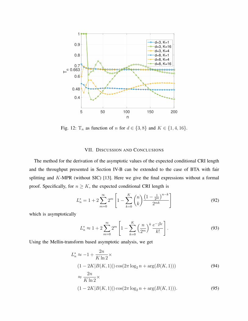
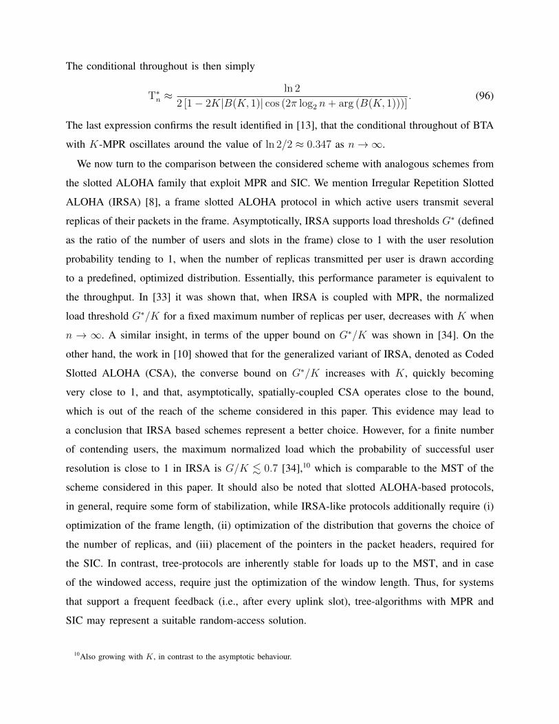
Finally, Fig. 12 shows the conditional throughput Tn for the combination of the splitting

factor d = {3, 8} and K ∈ {1, 4, 16}; again, the results are obtained by averaging over 10000

simulation runs. The already identified oscillatory behavior around the mean value (which are

roughly 0.663 and 0.48 for d = 3 and d = 8, respectively; see also Fig. 11) is clearly present

and the amplitude of the oscillations visibly amplifies with d (also compare with with Fig. 4.

However, the analysis of this interesting phenomenon is out of the paper scope.

5 50 100 150 200

n

0.4

0.48

0.6

0.6630.7

0.8

0.9

1

Tn

d=3, K=1d=3, K=16d=3, K=4d=8, K=1d=8, K=4d=8, K=16

Fig. 12: Tn as function of n for d ∈ {3, 8} and K ∈ {1, 4, 16}.

VII. DISCUSSION AND CONCLUSIONS

The method for the derivation of the asymptotic values of the expected conditional CRI length

and the throughput presented in Section IV-B can be extended to the case of BTA with fair

splitting and K-MPR (without SIC) [13]. Here we give the final expressions without a formal

proof. Specifically, for n ≥ K, the expected conditional CRI length is

L∗n = 1 + 2∞∑m=0

2m

[1−

K∑k=0

(n

k

)(1− 1

2m

)n−k2mk

](92)

which is asymptotically

L∗n ≈ 1 + 2∞∑m=0

2m

[1−

K∑k=0

( n2m

)k e− n2m

k!

]. (93)

Using the Mellin-transform based asymptotic analysis, we get

L∗n ≈ −1 +2n

K ln 2×

(1− 2K|B(K, 1)|) cos(2π log2 n+ arg(B(K, 1))) (94)

≈ 2n

K ln 2×

(1− 2K|B(K, 1)|) cos(2π log2 n+ arg(B(K, 1))). (95)

The conditional throughout is then simply

T∗n ≈ln 2

2 [1− 2K|B(K, 1)| cos (2π log2 n+ arg (B(K, 1)))]. (96)

The last expression confirms the result identified in [13], that the conditional throughout of BTA

with K-MPR oscillates around the value of ln 2/2 ≈ 0.347 as n→∞.

We now turn to the comparison between the considered scheme with analogous schemes from

the slotted ALOHA family that exploit MPR and SIC. We mention Irregular Repetition Slotted

ALOHA (IRSA) [8], a frame slotted ALOHA protocol in which active users transmit several

replicas of their packets in the frame. Asymptotically, IRSA supports load thresholds G∗ (defined

as the ratio of the number of users and slots in the frame) close to 1 with the user resolution

probability tending to 1, when the number of replicas transmitted per user is drawn according

to a predefined, optimized distribution. Essentially, this performance parameter is equivalent to

the throughput. In [33] it was shown that, when IRSA is coupled with MPR, the normalized

load threshold G∗/K for a fixed maximum number of replicas per user, decreases with K when

n → ∞. A similar insight, in terms of the upper bound on G∗/K was shown in [34]. On the

other hand, the work in [10] showed that for the generalized variant of IRSA, denoted as Coded

Slotted ALOHA (CSA), the converse bound on G∗/K increases with K, quickly becoming

very close to 1, and that, asymptotically, spatially-coupled CSA operates close to the bound,

which is out of the reach of the scheme considered in this paper. This evidence may lead to

a conclusion that IRSA based schemes represent a better choice. However, for a finite number

of contending users, the maximum normalized load which the probability of successful user

resolution is close to 1 in IRSA is G/K . 0.7 [34],10 which is comparable to the MST of the

scheme considered in this paper. It should also be noted that slotted ALOHA-based protocols,

in general, require some form of stabilization, while IRSA-like protocols additionally require (i)

optimization of the frame length, (ii) optimization of the distribution that governs the choice of

the number of replicas, and (iii) placement of the pointers in the packet headers, required for

the SIC. In contrast, tree-protocols are inherently stable for loads up to the MST, and in case

of the windowed access, require just the optimization of the window length. Thus, for systems

that support a frequent feedback (i.e., after every uplink slot), tree-algorithms with MPR and

SIC may represent a suitable random-access solution.

10Also growing with K, in contrast to the asymptotic behaviour.

Finally, we comment on an approach through which the performance of the scheme could be

pushed further. Specifically, as shown in [35], one of the factors limiting the performance of

tree algorithms with SIC is a too high fraction of singleton slots in comparison to IRSA-like

protocols, which are unavoidable due to the very nature of the collision resolution process. A

way to address this drawback and push the throughput performance is to form a set of partially-

split trees pertaining to the same initial collision and perform SIC over the whole set. It remains

to be seen how the addition of MPR to the framework would affect the performance of such

scheme.

REFERENCES

[1] J. Capetanakis, “Tree algorithms for packet broadcast channels,” IEEE Trans. Info. Theory, vol. 25, no. 5, pp. 505–515,

Sep. 1979.

[2] N. Abramson, “The ALOHA system – Another alternative for computer communications,” in Proc. of 1970 Fall Joint

Computer Conf., vol. 37. AFIPS Press, 1970, pp. 281–285.

[3] L. G. Roberts, “ALOHA packet system with and without slots and capture,” SIGCOMM Comput. Commun. Rev., vol. 5,

no. 2, pp. 28–42, Apr. 1975.

[4] S. Ghez, S. Verdu, and S. C. Schwartz, “Stability Properties of Slotted ALOHA with Multipacket Reception Capability,”

IEEE Trans. Autom. Control, vol. 33, no. 7, pp. 640–649, Jul. 1988.

[5] A. Zanella and M. Zorzi, “Theoretical Analysis of the Capture Probability in Wireless Systems with Multiple Packet

Reception Capabilities,” IEEE Trans. Commun., vol. 60, no. 4, pp. 1058–1071, Apr. 2012.

[6] J. Goseling, C. Stefanovic, and P. Popovski, “A Pseudo-Bayesian Approach to Sign-Compute-Resolve Slotted ALOHA,”

in Proc. IEEE ICC 2015, MASSAP Workshop, London, UK, Jun. 2015.

[7] E. Paolini, C. Stefanovic, G. Liva, and P. Popovski, “Coded random access: How coding theory helps to build random

access protocols,” IEEE Commun. Mag., vol. 53, no. 6, pp. 144–150, Jun. 2015.

[8] G. Liva, “Graph-based analysis and optimization of contention resolution diversity slotted ALOHA,” IEEE Trans. Commun.,

vol. 59, no. 2, pp. 477–487, Feb. 2011.

[9] E. Paolini, G. Liva, and M. Chiani, “Coded slotted ALOHA: A graph-based method for uncoordinated multiple access,”

IEEE Trans. Info. Theory, vol. 61, no. 12, pp. 6815–6832, Dec. 2015.

[10] C. Stefanovic, E. Paolini, and G. Liva, “Asymptotic Performance of Coded Slotted ALOHA with Multi Packet Reception,”

IEEE Commun. Lett., vol. 22, no. 1, pp. 105–108, Jan. 2018.

[11] Y. Yu and G. B. Giannakis, “High-Throughput Random Access Using Successive Interference Cancellation in a Tree

Algorithm,” IEEE Trans. Info. Theory, vol. 53, no. 12, pp. 4628–4639, Dec. 2007.

[12] S. Verdu, “Computation of the efficiency of the mosely-humblet contention resolution algorithm: A simple method,”

Proceedings of the IEEE, vol. 74, no. 4, pp. 613–614, Apr. 1986.

[13] C. Stefanovic, H. M. Gursu, Y. Deshpande, and W. Kellerer, “Analysis of Tree-Algorithms with Multi-Packet Reception,”

in Proc. IEEE GLOBECOM 2020, Taipei, Taiwan, Dec. 2020.

[14] P. Mathys and P. Flajolet, “Q-ary Collision Resolution Algorithms in Random-Access Systems with Free or Blocked

Channel Access,” IEEE Trans. Info. Theory, vol. 31, no. 2, pp. 217–243, Mar. 1985.

[15] J. L. Massey, “Collision-resolution algorithms and random-access communications,” in Multi-user communication systems.

Springer, 1981, pp. 73–137.

[16] B. S. Tsybakov, V. A. Mikhailov, and N. B. Likhanov, “Bounds for Packet Transmission Rate in a Random-Multiple-Access

System,” Probl. Peredachi Inf., vol. 19, no. 1, pp. 61–81, 1983.

[17] N. B. Likhanov, I. Plotnik, Y. Shavitt, M. Sidi, and B. S. Tsybakov, “Random Access Algorithms with Multiple Reception

Capability and n-ary Feedback Channel,” Probl. Peredachi Inf., vol. 29, no. 1, pp. 82–91, 1993.

[18] R.-H. Gau, “Tree/stack splitting with remainder for distributed wireless medium access control with multipacket reception,”

IEEE Trans. Wirel. Commun., vol. 10, no. 11, pp. 3909–3923, Nov. 2011.

[19] J. Goseling, C. Stefanovic, and P. Popovski, “Sign-Compute-Resolve for Tree Splitting Random Access,” IEEE Trans. Inf.

Theory, vol. 64, no. 7, pp. 5261–5276, Jul. 2018.

[20] G. T. Peeters and B. Van Houdt, “On the Maximum Stable Throughput of Tree Algorithms With Free Access,” IEEE

Trans. Info. Theory, vol. 55, no. 11, pp. 5087–5099, Nov. 2009.

[21] 3GPP, “TS36.321 v16.3.0 - Medium Access Control (MAC) protocol specification (Release 16).” Tech. Rep., Dec. 2020.

[22] E. Biglieri and L. Gyorfi, Eds., Multiple Access Channels. IOS press, 2007.

[23] O. Ordentlich and Y. Polyanskiy, “Low complexity schemes for the random access gaussian channel,” in Proc. IEEE ISIT

2017, Jun. 2017, pp. 2528–2532.

[24] S. Ghez, S. Verdu, and S. Schwartz, “Stability Properties of Slotted ALOHA with Multipacket Reception Capability,”

IEEE Trans. Automat. Contr., vol. 33, no. 7, pp. 640–649, Jul. 1988.

[25] L. Tong, Q. Zhao, and G. Mergen, “Multipacket reception in random access wireless networks: from signal processing to

optimal medium access control,” IEEE Commun. Maga., vol. 39, no. 11, pp. 108–112, Nov. 2001.

[26] A. Mengali, R. De Gaudenzi, and P. Arapoglou, “Enhancing the physical layer of contention resolution diversity slotted

ALOHA,” IEEE Trans. Commun., vol. 65, no. 10, pp. 4295–4308, Oct. 2017.

[27] D. Danyev, B. Laczay, and M. Ruszinko, “Multiple Access Adder Channel,” in Multiple Access Channels, E. Biglieri and

L. Gyorfi, Eds. IOS press, 2007, pp. 26–53.

[28] M. Al-Imari, P. Xiao, M. A. Imran, and R. Tafazolli, “Uplink non-orthogonal multiple access for 5G wireless networks,”

in Proc. IEEE ISWCS 2014, 2014.

[29] F. Clazzer, E. Paolini, I. Mambelli, and C. Stefanovic, “Irregular repetition slotted ALOHA over the Rayleigh block fading

channel with capture,” in Proc. IEEE ICC 2017, May 2017, pp. 1–6.

[30] P. Flajolet, X. Gourdon, and P. Dumas, “Mellin transforms and asymptotics: Harmonic sums,” Theor. Comput. Sci., vol.

144, pp. 3–58, 1995.

[31] D. E. Knuth, The Art of Computer Programming, 2nd ed. Addison - Wesley, 1998, vol. 3.

[32] A. Janssen and M. de Jong, “Analysis of contention tree algorithms,” IEEE Trans. Info. Theory, vol. 46, no. 6, pp.

2163–2172, 2000.

[33] M. Ghanbarinejad and C. Schlegel, “Irregular Repetition Slotted ALOHA with Multiuser Detection,” in Proc. IEEE WONS

2013, Banff, AB, Canada, Mar. 2013.

[34] I. Hmedoush, C. Adjih, P. Muhlethaler, and V. Kumar, “On the Performance of Irregular Repetition Slotted Aloha with

Multiple Packet Reception,” in Proc. IEEE IWCMC 2020, 2020, pp. 557–564.

[35] J. H. Sørensen, C. Stefanovic, and P. Popovski, “Coded splitting tree protocols,” in Proc. IEEE ISIT 2013, 2013, pp.

2860–2864.