Treatment of Constraint in Non-Linear Fracture Mechanics Noel O’Dowd Department of Mechanical and Aeronautical Engineering Materials and Surface Science Institute University of Limerick Ireland Bristol UK, June 20 th 2008 Acknowledgements: C. Fong Shih, S. Kamel. J. Sawyer, H. McGillivray, T. Tkazcyk

Welcome message from author
This document is posted to help you gain knowledge. Please leave a comment to let me know what you think about it! Share it to your friends and learn new things together.
Transcript
Treatment of Constraint in Non-Linear Fracture Mechanics
Noel O’DowdDepartment of Mechanical and Aeronautical Engineering
Materials and Surface Science InstituteUniversity of Limerick
Ireland
Bristol UK, June 20th 2008
Acknowledgements: C. Fong Shih, S. Kamel. J. Sawyer, H. McGillivray, T. Tkazcyk
2
Agenda
Motivation and Background
Discussion of higher order terms in crack tip fields
Application to idealised materials and geometries
Application to real conditions
3
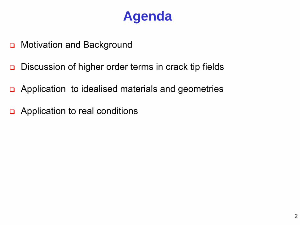
Variation in measured fracture toughness for ductile materials
Toughness ( JC) can depend on specimen geometry and size
10 mm
50 mm
25 mm
ASTM A515 from ECB specimens Kirk et al. 1991
50
150
200
250
300
350
0 0.0 0.1 0.2 0.3 0.4 0.5 0.6
100
Motivation
ECB = edge cracked benda: crack lengthW: specimen width
4
Motivation
J does not uniquely characterise material toughness
In standard practice a unique toughness value is ensured by
following size and geometry requirements for testing
However, requirements can lead to a very conservative toughness
and this motivated research into extending the J-based approach
5
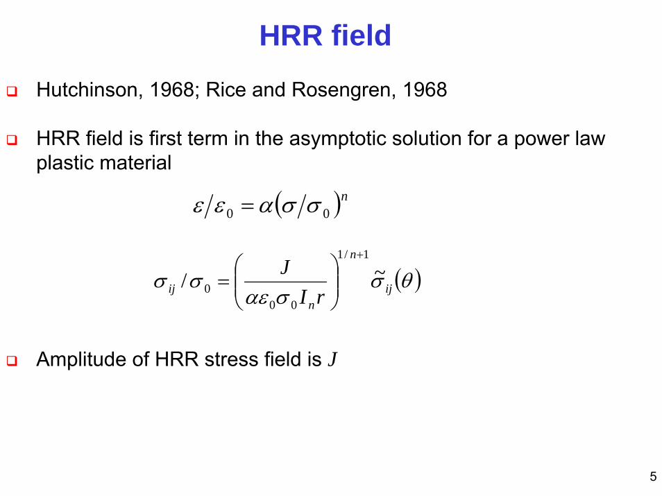
Hutchinson, 1968; Rice and Rosengren, 1968
HRR field is first term in the asymptotic solution for a power law plastic material
Amplitude of HRR stress field is J
HRR field
( )θσσαε
σσ ij
n
nij rI
J ~/1/1
000
+
⎟⎟⎠
⎞⎜⎜⎝
⎛=
( )n00 σσαεε =
6
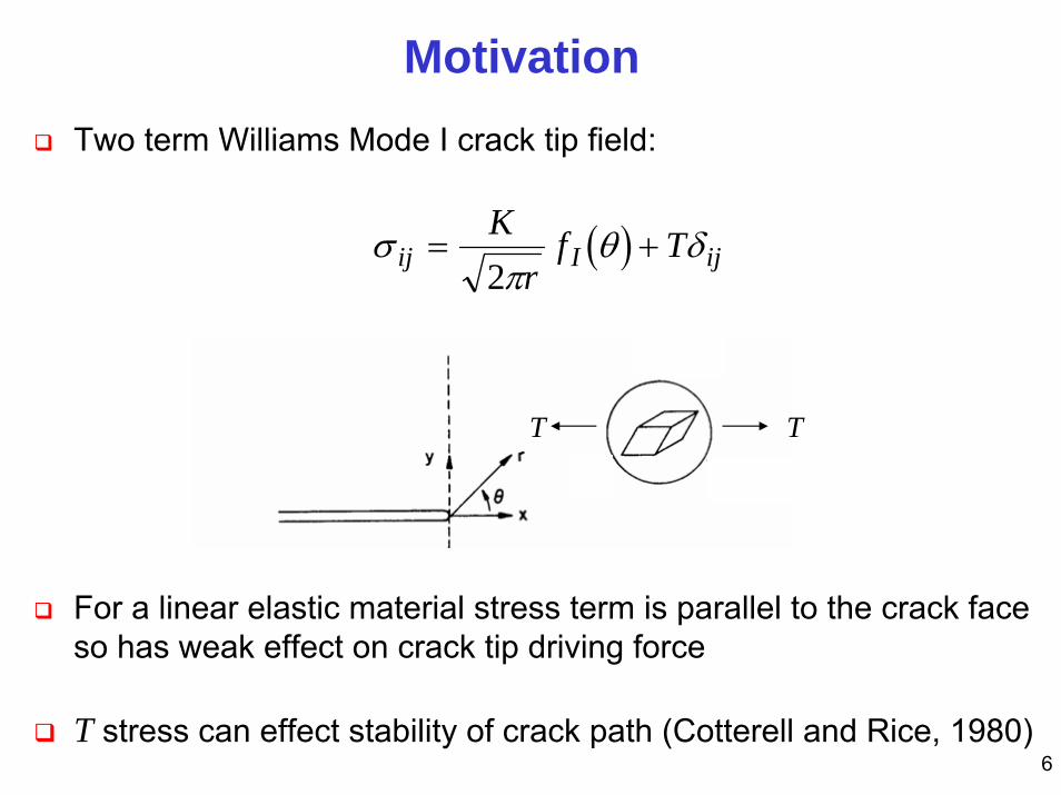
MotivationTwo term Williams Mode I crack tip field:
For a linear elastic material stress term is parallel to the crack face so has weak effect on crack tip driving force
T stress can effect stability of crack path (Cotterell and Rice, 1980)
( )σπ
θ δij I ijK
rf T= +
2
TT
7
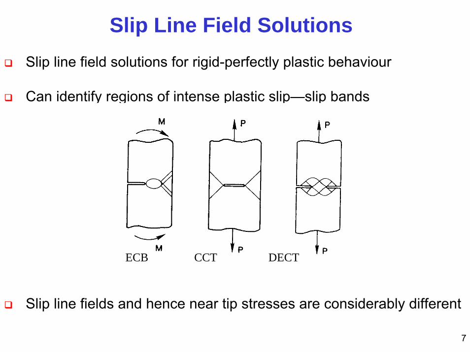
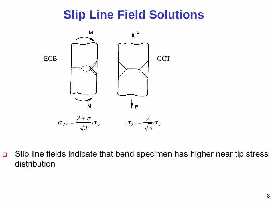
Slip line field solutions for rigid-perfectly plastic behaviour
Can identify regions of intense plastic slip—slip bands
Slip line fields and hence near tip stresses are considerably different
Slip Line Field Solutions
ECB CCT DECT
8
Slip line fields indicate that bend specimen has higher near tip stress distribution
Slip Line Field Solutions
ECB CCT
σ σ2223
= yσ π σ222
3=
+y
9
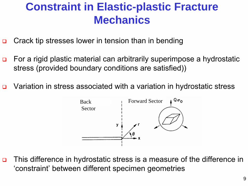
Crack tip stresses lower in tension than in bending
For a rigid plastic material can arbitrarily superimpose a hydrostatic stress (provided boundary conditions are satisfied))
Variation in stress associated with a variation in hydrostatic stress
This difference in hydrostatic stress is a measure of the difference in ‘constraint’ between different specimen geometries
Constraint in Elastic-plastic Fracture Mechanics
BackSector
Forward Sector
10
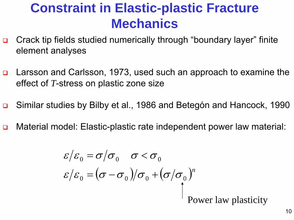
Crack tip fields studied numerically through “boundary layer” finite element analyses
Larsson and Carlsson, 1973, used such an approach to examine the effect of T-stress on plastic zone size
Similar studies by Bilby et al., 1986 and Betegón and Hancock, 1990
Material model: Elastic-plastic rate independent power law material:
Constraint in Elastic-plastic Fracture Mechanics
( ) ( )n0000
000
σσσσσεε
σσσσεε
+−=
<=
Power law plasticity
11
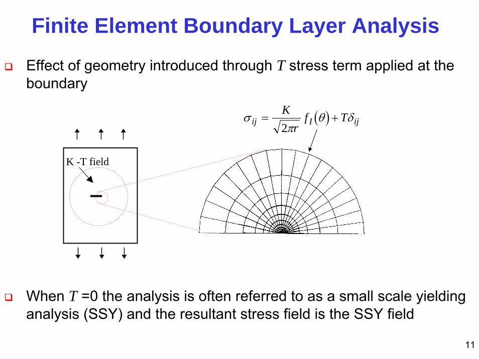
Effect of geometry introduced through T stress term applied at the boundary
When T =0 the analysis is often referred to as a small scale yielding analysis (SSY) and the resultant stress field is the SSY field
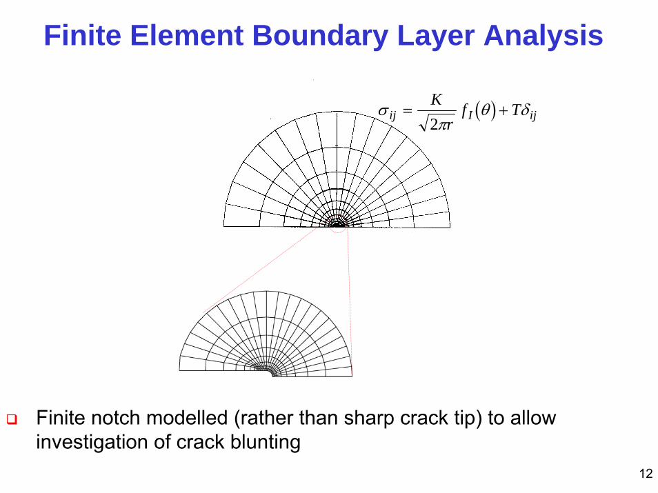
Finite Element Boundary Layer Analysis
( )σπ
θ δij I ijK
rf T= +
2
K -T field
12
Finite notch modelled (rather than sharp crack tip) to allow investigation of crack blunting
Finite Element Boundary Layer Analysis
( )σπ
θ δij I ijK
rf T= +
2
13
The T stress plays the role of a geometry parameter
By varying T/σ0 can generate a range of crack tip fields
T/σ0 = 0 corresponds (almost) to the HRR field
Finite strain analysis carried out to account for large deformations in the vicinity of the crack tip
Finite Element Boundary Layer Analysis

14
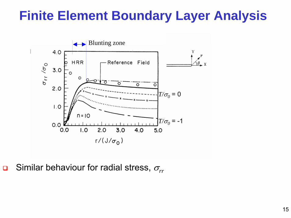
Stresses normalised by σ0; Distances normalised by J/σ0
J/σ0 is a measure of the crack tip opening and the crack blunting zone
Finite Element Boundary Layer Analysis
Blunting zone
T/σ0 = 0
T/σ0 = -1
T/σ0 = 1
15
Similar behaviour for radial stress, σrr
Finite Element Boundary Layer Analysis
Blunting zone
T/σ0 = -1
T/σ0 = 0
16
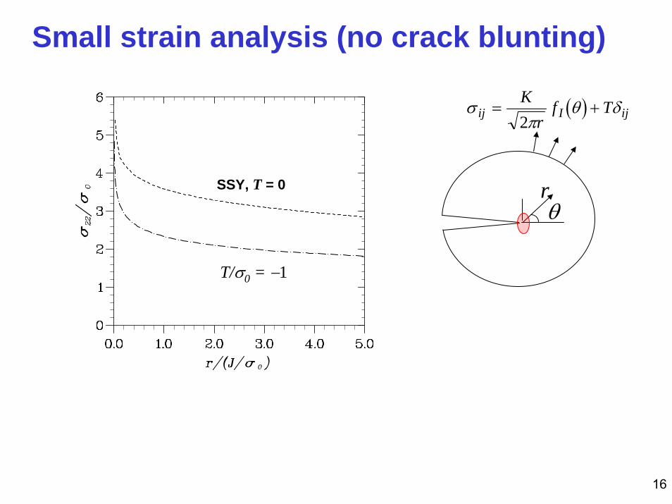
Small strain analysis (no crack blunting)
θrSSY, T = 0
T/σ0 = −1
( )σπ
θ δij I ijK
rf T= +
2
17
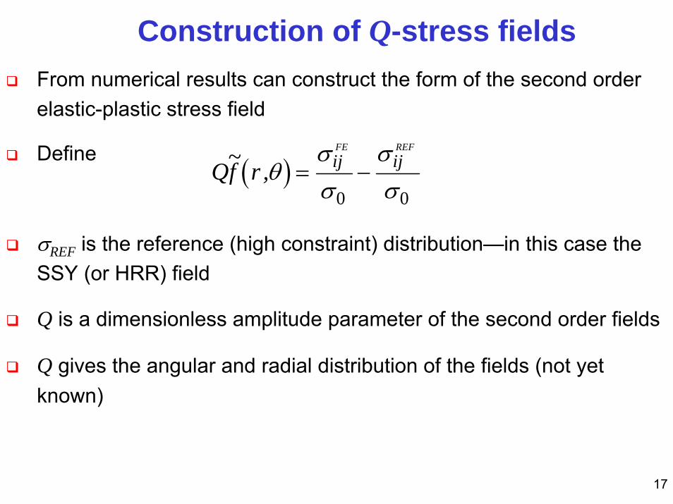
Construction of Q-stress fieldsFrom numerical results can construct the form of the second order elastic-plastic stress field
Define
σREF is the reference (high constraint) distribution—in this case the SSY (or HRR) field
Q is a dimensionless amplitude parameter of the second order fields
Q gives the angular and radial distribution of the fields (not yet known)
( )Qf r ij ijFE REF~ ,θ
σσ
σσ
= −0 0
18
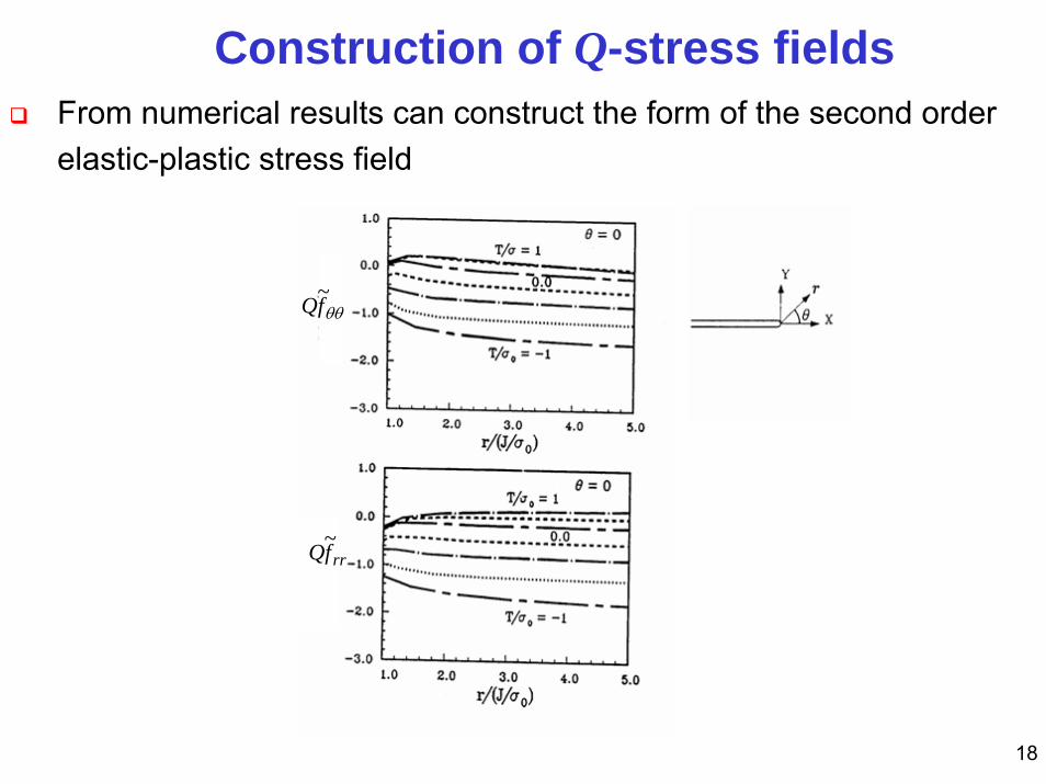
Construction of Q-stress fieldsFrom numerical results can construct the form of the second order elastic-plastic stress field
Qf~θθ
Qfrr~

19
Angular distribution:
To a good approximation:
Construction of Q-stress fields
0),(~1),(~),(~
=
==
θ
θθ
θ
θθ
rf
rfrf
r
rr
Qf~θθ Qfrr~ Qfr
~θ

20
Two parameter elastic-plastic stress fields
or, more generally
The parameter Q is a hydrostatic stress term determined from finite element analysis for the particular geometry and load level
ijref
ij Qδσ
σσσ +⎟⎟
⎠
⎞⎜⎜⎝
⎛=
00/
( )σ σαε σ
σ θ δijn
n
ij ijJ
I rQ/ ~
/
00 0
1 1
=⎛⎝⎜
⎞⎠⎟ +
+
21
SSY, T = 0
T/σ0 = −1
SSY, T = 0
T/σ0 = −1
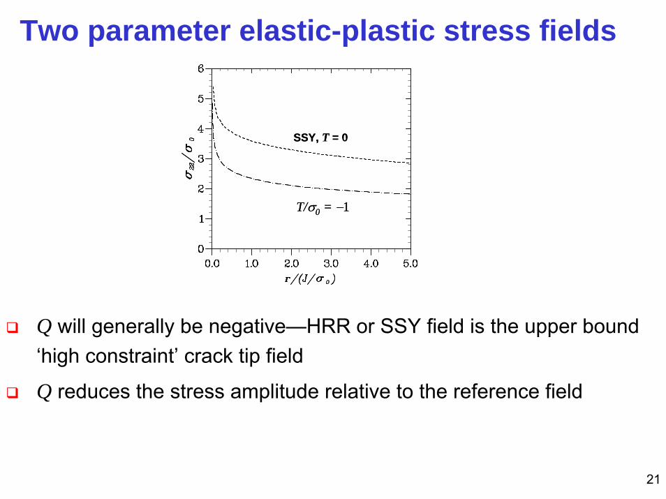
Q will generally be negative—HRR or SSY field is the upper bound ‘high constraint’ crack tip field
Q reduces the stress amplitude relative to the reference field
Two parameter elastic-plastic stress fields
22
Two Parameter Fracture Mechanics
Stress and strain fields depend on J and Q
Fracture toughness expressed in terms of JC(Q)
JIC is the standard high constraint fracture toughness value
corresponding to Q = 0 and is generally the lower bound
ijrefij Qδσσσσ += 00 //
23
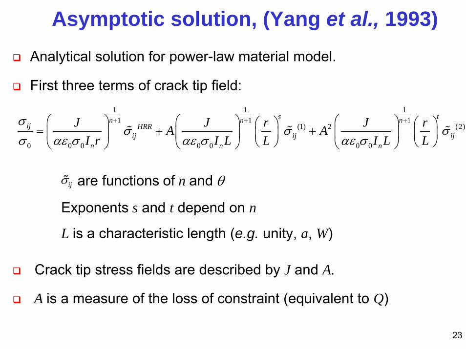
Asymptotic solution, (Yang et al., 1993)
1 1 11 1 1
(1) 2 (2)
0 0 0 0 0 0 0
s tn n nij HRR
ij ij ijn n n
J J r J rA AI r I L L I L L
σσ σ σ
σ αε σ αε σ αε σ
+ + +⎛ ⎞ ⎛ ⎞ ⎛ ⎞⎛ ⎞ ⎛ ⎞= + +⎜ ⎟ ⎜ ⎟ ⎜ ⎟⎜ ⎟ ⎜ ⎟⎝ ⎠ ⎝ ⎠⎝ ⎠ ⎝ ⎠ ⎝ ⎠
% % %
ijσ%
Analytical solution for power-law material model.
First three terms of crack tip field:
Exponents s and t depend on n
L is a characteristic length (e.g. unity, a, W)
are functions of n and θ
Crack tip stress fields are described by J and A.
A is a measure of the loss of constraint (equivalent to Q)
24
Two Parameter Fracture Mechanics
Analysis so far has been for idealised geometry, boundary layer analysis
Now consider ‘real’ geometries
25
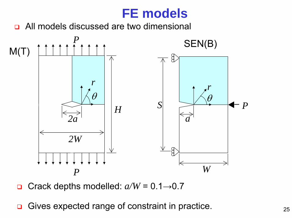
FE models
M(T)
Crack depths modelled: a/W = 0.1→0.7
Gives expected range of constraint in practice.
θr
2aH
2W
P
PAll models discussed are two dimensional
SEN(B)
aS P
θ
W
r
26
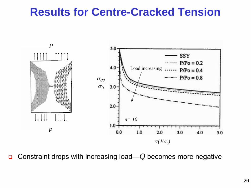
Constraint drops with increasing load—Q becomes more negative
Results for Centre-Cracked Tension
σσ
θθ
0
r/(J/σ0)
Load increasing
n= 10
P
P
27
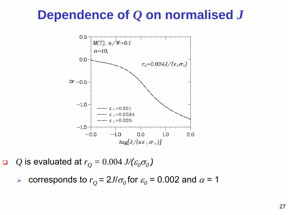
Dependence of Q on normalised J
Q is evaluated at rQ = 0.004 J/(ε0σ0 )
corresponds to rQ = 2J/σ0 for ε0 = 0.002 and α = 1
28
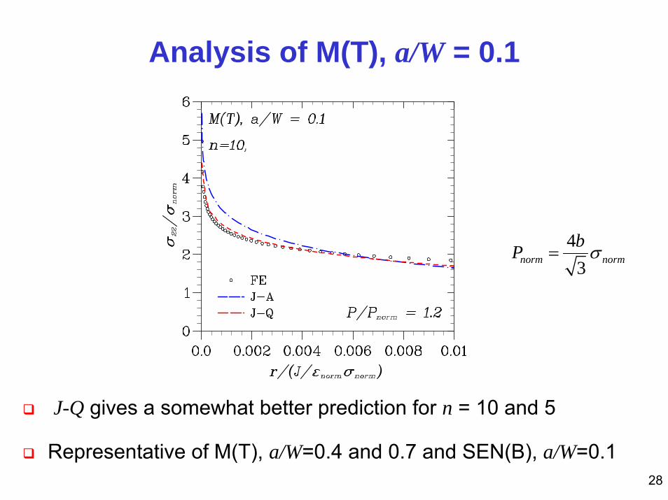
Analysis of M(T), a/W = 0.1
J-Q gives a somewhat better prediction for n = 10 and 5
Representative of M(T), a/W=0.4 and 0.7 and SEN(B), a/W=0.1
43norm normbP σ=
29
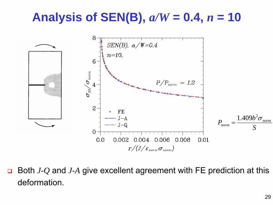
Analysis of SEN(B), a/W = 0.4, n = 10
Both J-Q and J-A give excellent agreement with FE prediction at this deformation.
21.409 normnorm
bPS
σ=
30
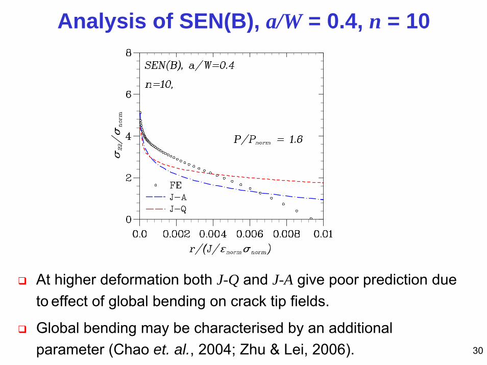
Analysis of SEN(B), a/W = 0.4, n = 10
At higher deformation both J-Q and J-A give poor prediction due to effect of global bending on crack tip fields.
Global bending may be characterised by an additional parameter (Chao et. al., 2004; Zhu & Lei, 2006).
31
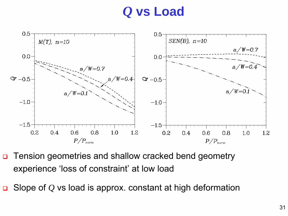
Q vs Load
Tension geometries and shallow cracked bend geometry experience ‘loss of constraint’ at low load
Slope of Q vs load is approx. constant at high deformation
32
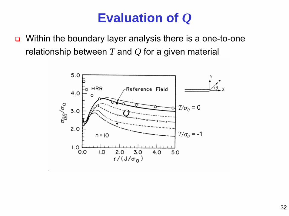
Evaluation of QWithin the boundary layer analysis there is a one-to-one relationship between T and Q for a given material
Q
T/σ0 = -1
T/σ0 = 0

33
Evaluation of Q
T is an elastic parameter and is relatively easily determined
Can thus estimate Q through an elastic analysis for T

34
Evaluation of QT stress can give a reasonable estimate of Q
Centre Cracked Tension Edge Cracked Panel

35
Power law estimates for Q
T-stress can be used to estimate Q under ‘small scale yielding’
conditions—when size of the plastic zone is small
Consider a pure power law material:
For such a material, stress at a point varies linearly with remote load
( )ε ε α σ σ/ /0 0= n
( ) ( )σ σ σ σ σij ij x n/ / ,0 0= ∞
36
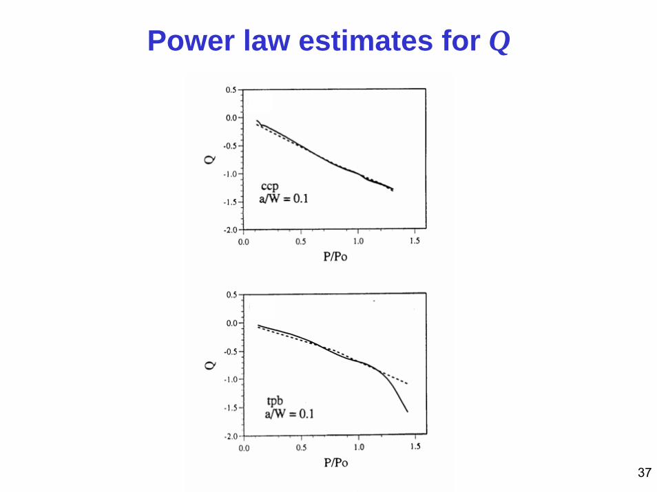
Power law estimates for QIt can be shown using the HRR field that
h1 is a function which depends only on geometry and n
Similarly it can be shown for a pure power law material
Q varies linearly with load
An approximation scheme based on T under small scale yielding
and h2 under extensive plasticity may then be used
( ) ( )Q h n= ∞σ σ/ 0 2
( ) ( )Ja
h nn
αε σσ σ
0 00
11= ∞ +
/
37
Power law estimates for Q
38
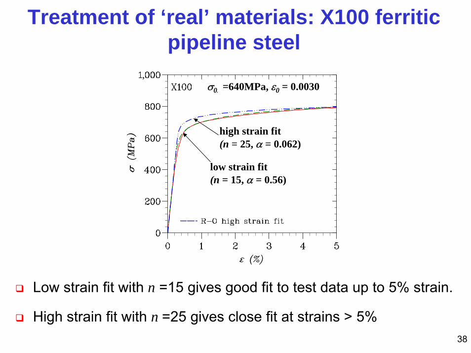
Treatment of ‘real’ materials: X100 ferritic pipeline steel
Low strain fit with n =15 gives good fit to test data up to 5% strain.
High strain fit with n =25 gives close fit at strains > 5%
σ0.2=640MPa, ε0 = 0.0030
low strain fit(n = 15, α = 0.56)
high strain fit(n = 25, α = 0.062)

39
Results for X100: M(T), a/W =0.1
J-Q gives best agreement with FE.
J-A prediction based on high strain fit gives better agreement than the low strain fit.
Kamel et al., 2007
40
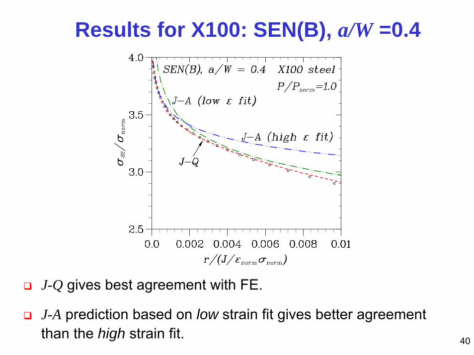
Results for X100: SEN(B), a/W =0.4
J-Q gives best agreement with FE.
J-A prediction based on low strain fit gives better agreement than the high strain fit.
41
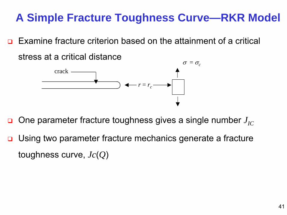
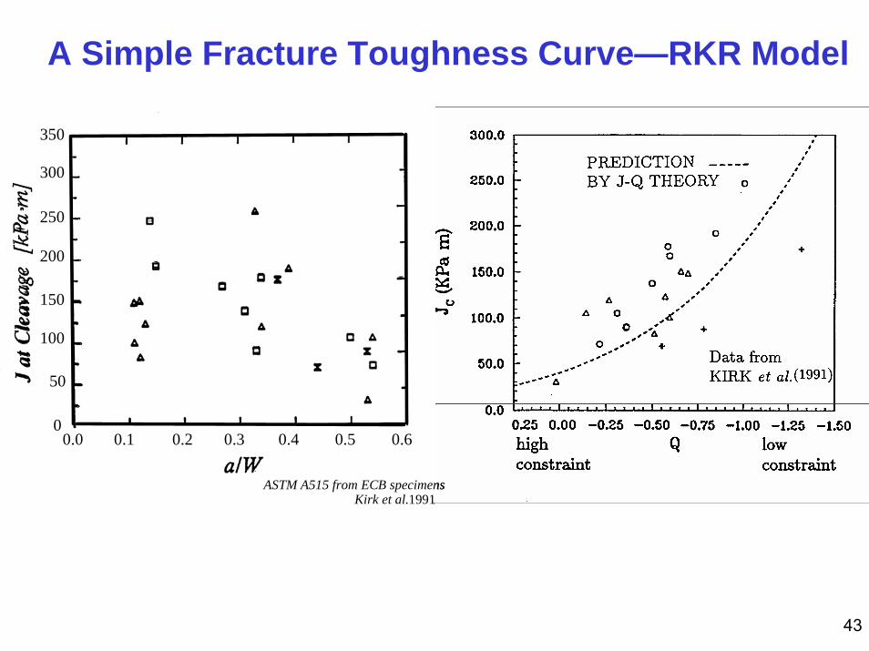
A Simple Fracture Toughness Curve—RKR Model
Examine fracture criterion based on the attainment of a critical
stress at a critical distance
One parameter fracture toughness gives a single number JIC
Using two parameter fracture mechanics generate a fracture
toughness curve, Jc(Q)
r = rc
σ = σc
crack
42
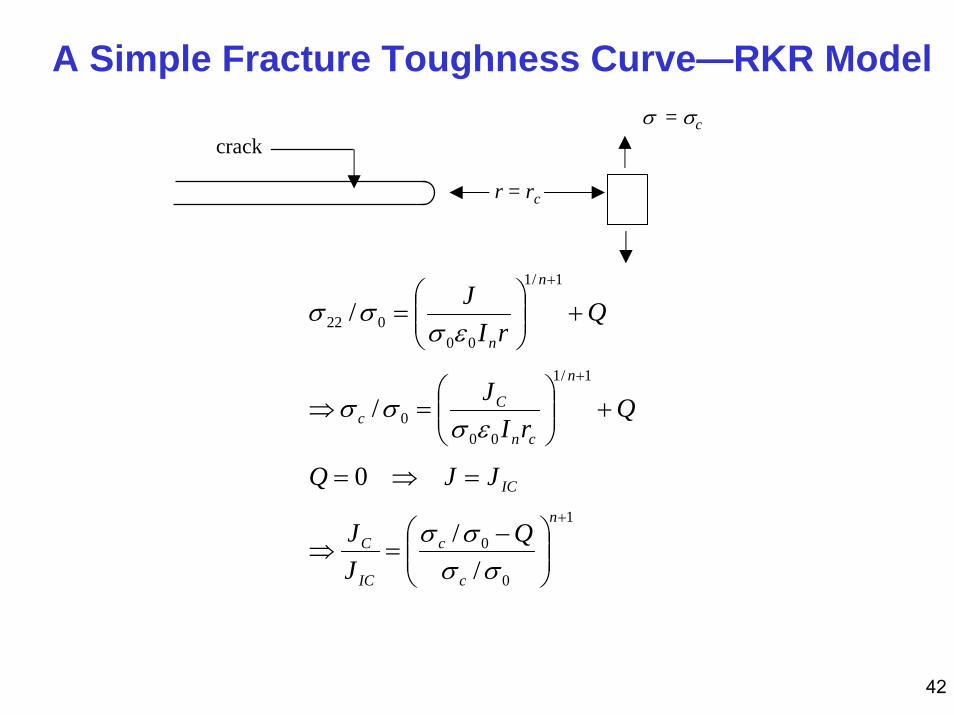
A Simple Fracture Toughness Curve—RKR Model
r = rc
σ = σc
crack
1
0
0
1/1
000
1/1
00022
//
0
/
/
+
+
+
⎟⎟⎠
⎞⎜⎜⎝
⎛ −=⇒
=⇒=
+⎟⎟⎠
⎞⎜⎜⎝
⎛=⇒
+⎟⎟⎠
⎞⎜⎜⎝
⎛=
n
c
c
IC
C
IC
n
cn
Cc
n
n
QJJ
JJQ
QrI
J
QrI
J
σσσσ
εσσσ
εσσσ
43
A Simple Fracture Toughness Curve—RKR Model
ASTM A515 from ECB specimensKirk et al.1991
50
150
200
250
300
350
00.0 0.1 0.2 0.3 0.4 0.5 0.6
100
ASTM A515 from ECB specimensKirk et al.1991
50
150
200
250
300
350
00.0 0.1 0.2 0.3 0.4 0.5 0.6
100
44
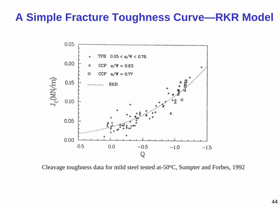
A Simple Fracture Toughness Curve—RKR Model
Cleavage toughness data for mild steel tested at-50oC, Sumpter and Forbes, 1992
45
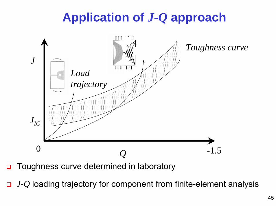
Application of J-Q approach
Toughness curve determined in laboratory
J-Q loading trajectory for component from finite-element analysis
J
Q0 -1.5
JIC
Toughness curve
Loadtrajectory
46
Alternative approach: Constraint matching
Estimate Q value at fracture for component
Test laboratory specimen with similar constraint level
Treat this fracture toughness as the ‘constraint’ matched toughness
E.g. For shallow cracked pipes under tension (Q ≈ −1) use fracture toughness Jc (or CTOD) from edge crack tension geometry
Approach widely used in offshore industry
47
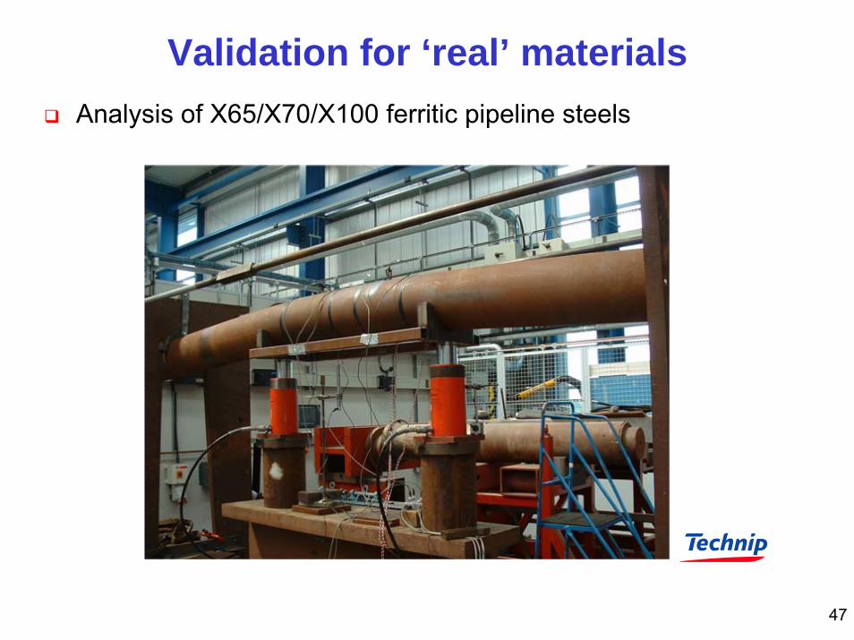
Validation for ‘real’ materialsAnalysis of X65/X70/X100 ferritic pipeline steels
48
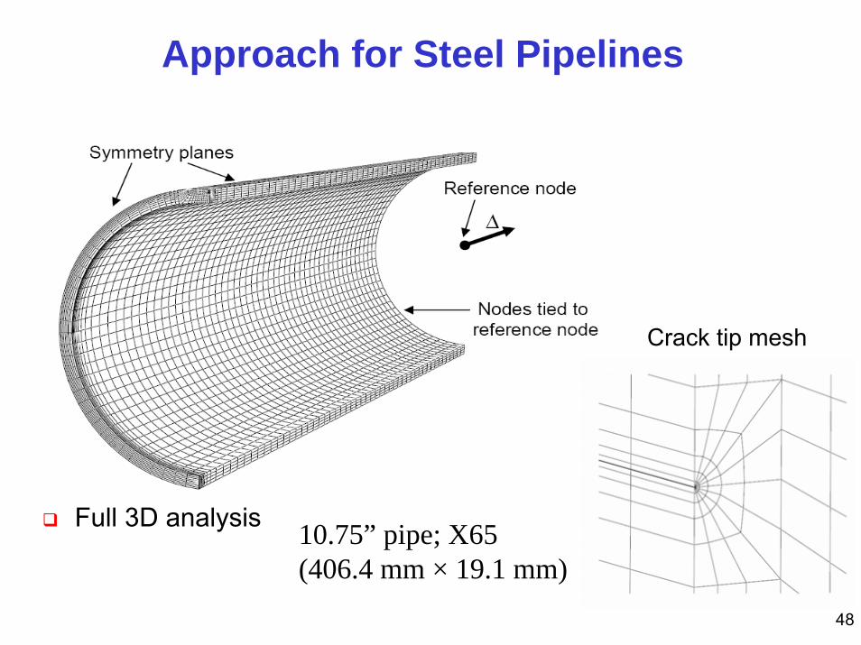
Approach for Steel Pipelines
Full 3D analysis
Crack tip mesh
10.75” pipe; X65(406.4 mm × 19.1 mm)
49
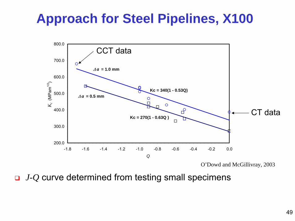
Approach for Steel Pipelines, X100
J-Q curve determined from testing small specimens
Kc = 340(1 - 0.53Q)
Kc = 270(1 - 0.63Q )
200.0
300.0
400.0
500.0
600.0
700.0
800.0
-1.8 -1.6 -1.4 -1.2 -1.0 -0.8 -0.6 -0.4 -0.2 0.0
Q
Kc
(MP
am1/
2 )
Δ a = 0.5 mm
Δ a = 1.0 mm
CT data
CCT data
O’Dowd and McGillivray, 2003
50
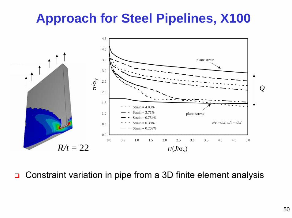
Approach for Steel Pipelines, X100
Constraint variation in pipe from a 3D finite element analysis
a/c =0.2, a/t = 0.2
0.0
0.5
1.0
1.5
2.0
2.5
3.0
3.5
4.0
4.5
0.0 0.5 1.0 1.5 2.0 2.5 3.0 3.5 4.0 4.5 5.0
Strain = 4.03%Strain = 2.71%Strain = 0.754%Strain = 0.38%Strain = 0.259%
plane strain
plane stress
σ/σ y
r/(J/σy)
Q
R/t = 22
51
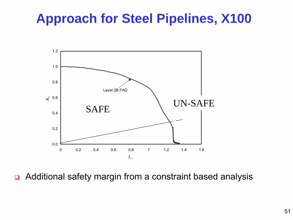
Approach for Steel Pipelines, X100
Additional safety margin from a constraint based analysis
0.0
0.2
0.4
0.6
0.8
1.0
1.2
0 0.2 0.4 0.6 0.8 1 1.2 1.4 1.6
L r
Kr
Level 2B FAD
Constraint modified Level 2B FAD
α = 0.5; β = -0.8
cutoff line
SAFE UN-SAFE
52
Conclusions
Crack tip driving force for an elastic-plastic material can be described by two parameters, J and Q
Q is a hydrostatic stress term, motivated by the form of the crack tip fields
Allowance for constraint can increase the safety margin or increase allowable load
Related Documents