Transversality theory, cobordisms, and invariants of symplectic quotients

arX

iv:m

ath/

0001

001v

1 [

mat

h.SG

] 1

Jan

200

0

Transversality theory, cobordisms,

and invariants of symplectic quotients

Shaun Martin∗

Introduction

Symplectic quotients and their invariants

This paper gives methods for understanding invariants of symplectic quotients. The sym-

plectic quotients that we consider are compact symplectic manifolds (or more generally

orbifolds), which arise as the symplectic quotients of a symplectic manifold by a compact

torus. A companion paper [23] examines symplectic quotients by a nonabelian group, show-

ing how to reduce to the maximal torus.

Throughout this paper we assume X is a symplectic manifold, and that a compact torus

T ∼= S1 × . . . × S1 acts on X , preserving the symplectic form, and having moment map

µ : X → t∗, where t∗ denotes the dual of the Lie algebra of T . We assume that µ is a proper

map. (For definitions and our sign conventions see the notation section at the end of this

introduction).

For every regular value p ∈ t∗ of the moment map, the inverse image µ−1(p) is a compact

submanifold of X which is stable under T , and on which the T -action is locally free (that

is, every point in µ−1(p) has finite stabilizer subgroup). The symplectic quotient, which we

denote X//T (p), is defined by taking the topological quotient by T

X//T (p) :=µ−1(p)

T,

and is a compact orbifold (it is a manifold if the stabilizer subgroup is the same for every

point in µ−1(p)). Moreover the symplectic form on X defines in a natural way a symplectic

form on X//T (p).

Many celebrated theorems in this field relate invariants of the triple (X,T, µ) to invariants

of the quotients X//T (p). For example, the Duistermaat-Heckman theorem [8] relates

a certain oscillatory integral over X to the volumes of the symplectic quotients X//T (p).

Another example is the Guillemin-Sternberg quantization theorem [12], which relates

the ‘geometric quantization’ of X to that of its symplectic quotients1. A third example is the

Atiyah-Guillemin-Sternberg convexity theorem, which relates a very simple invariant

of (X,T, µ), namely the convex hull of the finite set of points µ(XT ), to an even simpler

invariant of X//T (p), namely whether it is empty. One common feature of these results is

that the relevant invariants of (X,T, µ) can be calculated in terms of data localized at the

T -fixed points XT ⊂ X .

∗Institute for Advanced Study, Princeton, NJ; [email protected]; February, 1999.1the geometric quantization is the index of a certain naturally-defined Dirac operator; in the case of a

Kahler manifold this equals the space of holomorphic sections of a certain holomorphic line bundle

1

The scope of this paper

This paper provides results concerning a larger class of invariants, including the integrals

of arbitrary cohomology classes (thus generalizing the volume) and the indexes of arbitrary

elliptic differential operators (generalizing the geometric quantization). In order to describe

this class of invariants, we first note that any invariant of X//T (p) is also an invariant of the

pair (µ−1(p), T ) (the converse is of course not true). The easiest way to describe the results

of this paper is in terms of the submanifolds µ−1(p), for p any regular value of µ.

The submanifold µ−1(p) defines an equivalence class [µ−1(p)], defined in terms of certain

equivariant cobordisms, and the invariants accessible by the methods of this paper are those

invariants that only depend on the class [µ−1(p)].

Explicitly, let X ′ ⊂ X denote the subset consisting of those points whose stabilizer

subgroup is finite. Then the submanifold µ−1(p) ⊂ X ′ defines the cobordism class

[µ−1(p)] ∈ U∗T (X ′),

where representatives of U∗T (X ′) are given by T -equivariant maps of oriented manifolds

to X ′, and equivalences are given by the boundaries of T -equivariant maps of oriented

manifolds-with-boundary. Explicitly, if W → X ′ is any oriented manifold-with-boundary

mapped T -equivariantly to X ′, then [∂W → X ′] = 0 ∈ U∗T (X ′). Note that since X ′ has a

locally free T -action, every manifold and cobordism must also have a locally free T -action.

An example of an invariant that only depends on the class [µ−1(p)] is described in terms

of the natural ring homomorphism

κ : H∗T (X ; Q) ։ H∗

T (X//T (p); Q)

defined by restriction, followed by the natural identification of the equivariant cohomology

of µ−1(p) with the regular cohomology of its quotient. This map is often referred to as the

‘Kirwan map’, and is known to be surjective [21]. Given classes a, b ∈ H∗T (X), then Stokes’s

theorem implies that the ‘cohomology pairing’

H∗T (X)⊗H∗

T (X)→ Q

a, b 7→

∫

X//T (p)

κ(a) ⌣ κ(b)

is an invariant of the equivalence class [µ−1(p)] (Stokes’s theorem is also valid for orbifolds,

as we explain in appendix A). A similar map exists in K-theory, and again only depends

on the class [µ−1(p)]

The main result of this paper

We now describe the main topological result of this paper: theorem C (which appears in sec-

tion 8). Theorem C describes a cobordism between µ−1(p) and a collection of submanifolds

of X that lie near the T -fixed points:

Theorem C (Approximate version). Suppose the fixed point set XT is finite. Then for

every regular value p of the moment map,

[µ−1(p)] =∑

i∈I

[S(Fi)];

where each Fi ∈ XT is a fixed point, and S(Fi) is a d-fold product of odd-dimensional

spheres, lying in a small neighbourhood of Fi, with d = dimT .

2

In general, S(Fi) is a d-fold fibre product of sphere bundles over a connected component

Fi ⊂ XT of the fixed point set. Recall that, by definition, the equivalence class µ−1(p) is

defined in terms of submanifolds on which T has a locally free action. The quotient S(Fi)/T

is an orbifold, and can be described as a d-fold ‘tower’ of weighted projective bundles over

Fi.

By describing the submanifolds S(Fi) explicitly, we can calculate the cohomology pair-

ings described above in terms of data localized at the fixed points. Theorem D carries this

out, giving cohomological formulae in terms of characteristic classes.

It is also possible, by applying techniques in K-theory, to derive formulae for the indices

of elliptic operators: these formulae will appear in another paper.

Overview of the paper

This paper has four main results, theorems A, B, C, and D. Their logical relationship is as

follows (the numbers indicate sections)

Topology Cohomology

WallsTheorem A (1–4)

wall-crossing-cobordism+3

��

Theorem B (5–6)wall-crossing formula

��

Fixed pointsTheorem C (7–8)

fixed point cobordism+3 Theorem D (9)fixed point formula.

Theorem A is the main topological construction in this paper. Theorems A and C each

give a cobordism between µ−1(p) and a collection of ‘simpler’ spaces: in theorem C each such

space is a d-fold fibre product of sphere bundles over a component of XT , where d = dimT ;

in theorem A each such space is a sphere bundle over a submanifold of a manifold XH ,

where H ⊂ T is a 1-dimensional subtorus. In fact XH is a symplectic manifold, with an

action of the (d − 1)-torus T/H , and having a moment map µ′. The submanifold of XH

which appears in theorem A is µ′−1(q), for q some regular value of µ′. Theorem A forms

the inductive step in the proof of theorem C, and the induction is carried out in sections

7 and 8. The main techniques used in the proofs of theorems A and C are transversality

theory, and general results in the theory of Lie group actions on manifolds. The symplectic

geometry which is used boils down to a single fact, fact 1.1, which is illustrated in figure 1.

Theorems B and D result from applying cohomological techniques to the cobordisms

constructed in theorems A and C. Whereas a naive application of Stokes’s theorem would

result in formulae which were computable in principle, but unwieldy in practise, the real

content of theorems B and D is to show how such formulae can be reduced to computable

formulae, eventually in terms of only the fixed points of X . This is explained in more detail

at the beginning of section 5. In the proofs of theorems B and D, fairly extensive use is made

of techniques in equivariant cohomology. We also use various facts about orbifolds, which

are explained in appendix A, as well as formulae which calculate integrals over the fibres

of weighted projective bundles. These formulae are proved in appendix B, and generalize

classical formulae involving Chern classes and Segre classes.

Finally, sections 11 and 12 calculate some explicit examples. In section 11 we study the

n-fold product of 2-spheres (S2)n. This is a symplectic manifold, with a Hamiltonian action

3

of SO(3), and the symplectic quotient (S2)n//SO(3)(0) is a manifold when n is odd. These

symplectic quotients have been studied extensively, beginning with Kirwan’s determination

of the Betti numbers [21, 18, 13]. We use theorem B, together with an integration formula

which allows us to reduce from a symplectic quotient by SO(3) to a symplectic quotient by

the maximal torus S1 (proved in a companion paper [23]) to give the following formula for

integrals of arbitrary cohomology classes on the symplectic quotient (S2)n//SO(3)(0), for n

odd:∫

(S2)n//SO(3)(0)

vl11 ⌣ vl22 ⌣ . . . ⌣ vlnn = −1

2(−1)

n−12

∑

K⊂{1...n−1}

|K|=n−12

(−1)|K∩{1...m}|

where∑

i li = n− 3 and m is equal to the number of odd li, and vi is the natural degree 2

cohomology class arising from the i-th sphere in the product.

In section 12 we consider the space (CP2)n. This has a Hamiltonian action of SU(3),

and we calculate the volume of the symplectic quotient (CP2)n//SU(3)(0) (the formula is

not very enlightening, but the methods are an application of theorem D).

Relationship to other results

There are a number of relationships between the cohomological formulae proved in this

paper (theorems B and D) and results of other authors.

The mathematics in this paper was worked out in 1994, in Oxford and at the Newton

Institute in Cambridge. The intervening years have been partly spent trying (possibly un-

successfully) to understand how to turn raw mathematics into a comprehensible manuscript.

However, this is a first attempt at writing mathematics, and so I beg the readers indulgence

in judging it.

The nonabelian localization formula of Witten [29] and Jeffrey-Kirwan [14] gives an al-

ternative way of calculating cohomology pairings on symplectic quotients, involving residues

when T = S1, and a multidimensional generalization of the residue when dimT > 1.

An alternative approach to the Witten-Jeffrey-Kirwan cohomology formula was taken by

Guillemin and Kalkman [10], following from earlier independent work of Kalkman [17].

Guillemin and Kalkman use ‘symplectic cutting’ and ‘reduction in stages’, but the geomet-

ric arguments bear a strong resemblance to some of the arguments of this paper.

Jeffrey and Kirwan used the wall-crossing formula (theorem B in this paper, also the

main result in Guillemin-Kalkman [10]), together with results in the companion paper [23]

to give a mathematically rigorous proof of Witten’s formulae for cohomology pairings on

the moduli spaces of stable holomorphic bundles over a Riemann surface described above.

Some independent results on cobordisms of symplectic manifolds have also been an-

nounced by Ginzburg, Guillemin and Karshon [9].

Acknowledgements

I have benefited from very many elightening conversations with Simon Donaldson, Mario

Micallef, Frances Kirwan, Mike Alder, Michael Callahan, Stuart Jarvis, Allen Knutson,

Rebecca Goldin, Haynes Miller, and Victor Guillemin. But above all, I owe a great debt of

gratitude to Dietmar Salamon who has been both a friend and source of inspiration to me.

4

Contents

1 Constructing the wall-crossing-cobordism 8

Prelude: the geometry of the moment map . . . . . . . . . . . . . . . . . . . . . . . 8

The main lemma, and the resulting construction . . . . . . . . . . . . . . . . . . . . . 10

A combinatorial characterization of transverse paths, and the proof of Proposition 1.5 11

2 The data of a path, and how it describes the boundary of the wall-crossing-

cobordism 12

The data associated to a transverse path . . . . . . . . . . . . . . . . . . . . . . . . . 12

The boundary of the wall-crossing-cobordism . . . . . . . . . . . . . . . . . . . . . . 13

The boundary components as weighted projective bundles . . . . . . . . . . . . . . . . 13

3 The orbifold singularities and orientation of the wall-crossing-cobordism 15

Orbifold singularities in the wall-crossing-cobordism . . . . . . . . . . . . . . . . . . . 15

Orienting the wall-crossing-cobordism . . . . . . . . . . . . . . . . . . . . . . . . . . 16

4 Theorem A: a summary of the existence and properties of the wall-crossing-

cobordism. 17

5 The localization map and the wall-crossing formula 18

6 The wall-crossing formula in terms of characteristic classes 21

7 A generalization of a transverse path and its data 22

A τ -transverse path and its data . . . . . . . . . . . . . . . . . . . . . . . . . . . . . 22

The module of relations . . . . . . . . . . . . . . . . . . . . . . . . . . . . . . . . . . 23

8 Cobordisms between symplectic quotients and bundles over the fixed points 24

The spaces involved . . . . . . . . . . . . . . . . . . . . . . . . . . . . . . . . . . . . 25

The cobordism theorem . . . . . . . . . . . . . . . . . . . . . . . . . . . . . . . . . . 26

The structure of the spaces P(Θ,q) . . . . . . . . . . . . . . . . . . . . . . . . . . . . 28

9 Localizating integration formulae to the fixed points 29

A formula for λΘ in terms of characteristic classes . . . . . . . . . . . . . . . . . . . . 30

10 A more refined look at the module of relations 31

11 Calculations I: cohomology pairings on symplectic quotients of (S2)n 32

The moment map . . . . . . . . . . . . . . . . . . . . . . . . . . . . . . . . . . . . . 32

The integration formula relating the symplectic quotients by a nonabelian group and

by its maximal torus . . . . . . . . . . . . . . . . . . . . . . . . . . . . . . . . . 33

The volume of the symplectic quotient . . . . . . . . . . . . . . . . . . . . . . . . . . 33

The calculation . . . . . . . . . . . . . . . . . . . . . . . . . . . . . . . . . . . . . . 34

Cohomology classes on (S2)n. . . . . . . . . . . . . . . . . . . . . . . . . . . . . . . 35

12 Calculations II: volume of the symplectic quotient of (CP2)n 37

Generalities on CPk−1 . . . . . . . . . . . . . . . . . . . . . . . . . . . . . . . . . . . 37

Calculations on (CP2)n . . . . . . . . . . . . . . . . . . . . . . . . . . . . . . . . . . 39

The Volume . . . . . . . . . . . . . . . . . . . . . . . . . . . . . . . . . . . . . . . . 42

5

A Orbifolds, orbifold-fibre-bundles, and integration over the fibre 43

The definition of an orbifold . . . . . . . . . . . . . . . . . . . . . . . . . . . . . . . 44

The fundamental class of an oriented orbifold . . . . . . . . . . . . . . . . . . . . . . 44

Oriented orbifolds with boundary and Stokes’s theorem . . . . . . . . . . . . . . . . . 45

Orbibundles and integration over the fibre . . . . . . . . . . . . . . . . . . . . . . . . 45

How orbifold-fibre-bundles can arise as locally free quotients of manifolds . . . . . . . 47

B Cohomology and integration formulae for weighted projective bundles 48

Projective bundles . . . . . . . . . . . . . . . . . . . . . . . . . . . . . . . . . . . . . 48

Weighted Chern classes and the cohomology formula . . . . . . . . . . . . . . . . . . 49

Weighted Segre classes and the integration formula . . . . . . . . . . . . . . . . . . . 52

Equivariant weighted Segre classes, and the equivariant integration formula . . . . . . 54

C Proof of the orientation lemma 55

Notation and conventions

Fixed through the entire paper, are the following:

X is a fixed smooth symplectic manifold (with symplectic form ω);

T ∼= S1 × . . .× S1 is a compact torus acting smoothly on X , preserving ω;

t, t∗ are the Lie algebra of T and its dual, respectively;

µ : X → t∗ is a moment map for the T action on X (we will assume throughout that

µ is proper).

We will use the following notational conventions:

X//T (p) = µ−1(p)/T denotes the ‘symplectic quotient of X by T at p’;

XH denotes the subset of points fixed by the subgroup H ⊂ T ;

H∗(−) will always denote cohomology with rational coefficients;

H∗G(−) denotes G-equivariant cohomology (rational coefficients) for G a group;

κ : H∗T (X)→ H∗(X//T (p)) for p a regular value of the moment map, denotes the nat-

ural map given by first restricting to µ−1(p), and then applying the natural

isomorphism H∗T (µ−1(p)) ∼= H∗(X//T (p)) (the point p will always be clear from

the context). κ is often referred to as the Kirwan map.

Sign conventions for the moment map

Different authors use varying sign conventions for the moment map. Ours will be as fol-

lows. Given a symplectic manifold (X,ω) with an action of a torus T ∼= S1 × . . . × S1 by

symplectomorphisms, let V : t→ Γ(TX) be the infinitesimal action map, taking an element

ξ of the Lie algebra of T to the corresponding vector field V (ξ) on X . Then µ : X → t∗

is a moment map if it intertwines the T -action on X and the coadjoint action of T on t∗

(which is trivial in our case, since T is abelian), and which satisfies

〈dµx(v), ξ〉 = ωx(V (ξ), v), ∀x ∈ X, v ∈ TxX, ξ ∈ t. (0.1)

An almost complex structure J : TX → TX is compatible with ω if

g(·, ·) := ω(·, J ·) (0.2)

6

defines a Riemannian metric on X (i.e. if g is symmetric and positive-definite).

In the case of S1 ⊂ C∗ acting on C by multiplication, our conventions boil down to the

following. Letting z = x+ iy, and choosing the symplectic form

ω = dx ∧ dy,

then the standard complex structure on C is compatible with ω, and a moment map for the

S1-action is given by

µ(z) = −1

2|z|2.

Finally, we recall the standard orientation of a complex vector space, as defined in

algebraic geometry: if {e1, . . . , en} is a complex basis, then

{e1, ie1, e2, ie2, . . . en, ien} (0.3)

is a real oriented basis. Thus, if X is a symplectic manifold and J is a compatible almost

complex structure, the orientation induced by J agrees with the orientation given by the

top power of the symplectic form.

7

1. Constructing the wall-crossing-cobordism

This section contains the main construction of the paper: the construction of the ‘wall-

crossing-cobordism’. The tools needed for this construction comprise one fact from sym-

plectic geometry, and some transversality theory. We begin by stating the fact from sym-

plectic geometry, and illustrating it with a simple example. We then go on to the main

construction.

Prelude: the geometry of the moment map

We begin by explaining the key fact from symplectic geometry that we use in this paper:

this fact relates submanifolds defined by the group action to submanifolds defined by critical

points of the moment map.

µ

X

XH0

XH1

XT

µ(XH0 )

µ(XH1 )µ(XT )

Lie(T/H0)∗

Lie(T/H1)∗

Lie(T/H2)∗

t∗t∗

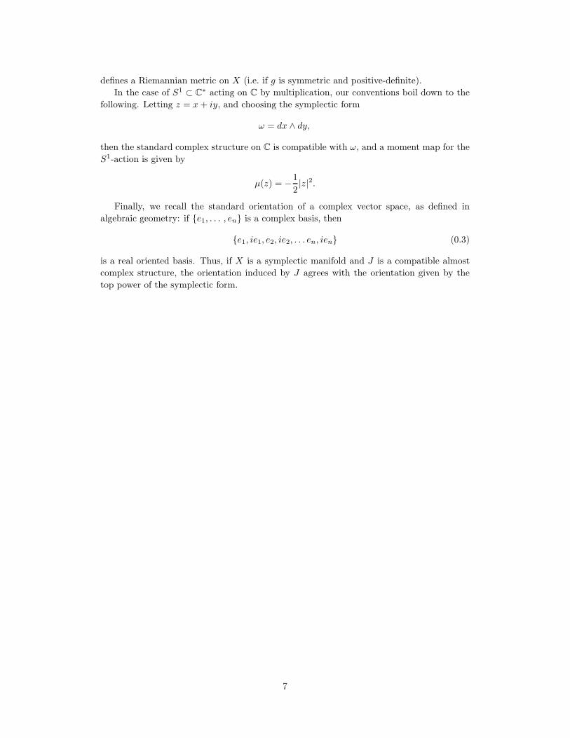
Figure 1: A moment map, and its restriction to various submanifolds: illustrating fact 1.2. Here T is

2-dimensional, and the subgroups Hi are 1-dimensional subtori. The manifold X and its submanifolds

are only represented schematically: in the concrete example from which this illustration is derived, X is

6-dimensional, and each component of XHi (represented by a curved line in X) is a 2-sphere (explained in

example 1.3).

Recall that X denotes a symplectic manifold, acted on by a torus T ∼= S1 × . . . × S1,

with associated moment map µ : X → t∗, where t∗ denotes the dual of the Lie algebra of T .

Let τ ⊂ T be a subtorus. Then the short exact sequence of groups τ → T ։ T/τ induces

the following exact sequences of Lie algebras and their duals

Lie(τ) → t ։ Lie(T/τ)

Lie(τ)∗ և t∗ ← Lie(T/τ)∗.

Hence for any subtorus τ we will consider Lie(T/τ)∗ to be a subspace of t∗ (of codimension

dim τ).

The key fact concerning the geometry of µ describes the way that the derivative of µ

encodes information about the T action. For any point x ∈ X , letting dµ : TxX → t∗ denote

the derivative, we have

8

Fact 1.1 (Infinitesimal version). A subtorus τ ⊂ T fixes x if and only if

dµ(TxX) ⊂ Lie(T/τ)∗.

For example, if the action is locally free at x, then dµx must be onto, and hence if p ∈ t∗

is a regular value of µ, then the action on T on µ−1(p) is locally free.

The above fact has a global consequence. If τ ⊂ T is a subtorus, then we denote by

Xτ the set of points fixed by τ : a local-coordinate argument shows that Xτ is a closed

submanifold of X (and an averaging argument shows that Xτ is a symplectic submanifold

of X).

Fact 1.2 (Global version). The moment map µ maps each component of Xτ to an affine

translate of Lie(T/τ)∗ in t∗.

For example, fixing a 1-dimensional subtorus H ∼= S1 of T , then µ maps each connected

component of XH to an affine hyperplane in t∗, parallel to Lie(T/H)∗. The images of such

submanifolds XH , as H varies through all 1-dimensional subtori of T , form ‘walls’ which

separate regions of regular values in µ(X). At the other extreme, µ maps each connected

component of XT to a point in t∗.

Example 1.3. Let X be the set of 3 × 3 Hermitian matrices with eigenvalues 0, 1 and 4,

and let T ⊂ SU(3) be the maximal torus. Then T acts on X by conjugation, and a moment

map for this action is given by sending a matrix to its diagonal entries. Figure 1 illustrates

some of the features of the moment map in this case (the image of the moment map is

accurate, but the illustration of X is schematic: X is 6-dimensional). The details in this

illustration are explained below.

We describe X and T explicitly as follows. Let T be the diagonal matrices in SU(3),

that is, T = {diag(eiθ0 , eiθ1 , eiθ2) | θ1 +θ2 +θ3 = 0}, and let t ∈ T act on a matrix A ∈ X by

A 7→ tAt−1. The map which takes A ∈ X to its diagonal entries (a11, a22, a33) takes values

in a 2-dimensional hyperplane in R3 (since a11 + a22 + a33 = trA = 5), and this hyperplane

can then be identified with t∗ to give a moment map for the T -action (the symplectic form

on X is defined by identifying X with a certain coadjoint orbit2).

The set of T -fixed points in X are the diagonal matrices: the diagonal entries must be

0, 1, 4 in some order, and so there are 6 such matrices. That is, XT consists of 6 isolated

points. These points and their images under µ are depicted in the lower right part of figure 1.

The Atiyah-Guillemin-Sternberg convexity theorem states that the image µ(X) equals the

convex hull of the image µ(XT ) of these points. Note that the example we are considering is

atypical, because each point of µ(XT ) defines a vertex of the polyhedron µ(X). In general,

not every point in µ(XT ) defines a vertex: some may map to the interior of µ(X).

Now consider the 1-dimensional subtorus H0 := {diag(eiθ0 , e−iθ0/2, e−iθ0/2} ⊂ T . Then

H0 fixes the ‘block-diagonal’ matrices of the form

b 0 0

0 ∗ ∗

0 ∗ ∗

.

The entry b must be one of the eigenvalues 0, 1 or 4, and the remaining 2 × 2 block has

eigenvalues given by the other two. Thus XH0 is made up of three components (each

such component turns out to be a 2-sphere). A similar analysis holds for the subtori

2The map A 7→ iA identifies X with an adjoint orbit of U(3); using an invariant inner product to identify

Lie(U(3)) ∼= Lie(U(3))∗ then identifies X with a coadjoint orbit, on which there is a natural symplectic

form. A moment map for the T -action is then given by the composition X → Lie(U(3))∗ ։ Lie(T )∗.

9

H1 := {diag(e−iθ1/2, eiθ1 , e−iθ1/2} and H2 := {diag(e−iθ2/2, e−iθ2/2, eiθ2}. There are in-

finitely many 1-dimensional subtori of T : all the others have as their fixed points only the

points XT .

In figure 1 the subspaces Lie(T/Hi) ⊂ t∗ are shown (here 0 ≤ i ≤ 2). Since each Hi has

dimension 1, these subspaces have codimension 1: they are hyperplanes. Each submanifold

XHi has three components, each of which maps to an affine translate of Lie(T/Hi) (shown

for i = 0, 1, the picture for i = 2 is similar).

The main lemma, and the resulting construction

Definition 1.4. Let p0 and p1 be regular values of the moment map µ : X → t∗. A

transverse path is a one-dimensional submanifold Z ⊂ t∗, with boundary {p0, p1}, such

that Z is transverse to µ.

It follows from transversality theory that µ−1(Z) is a submanifold of X , with boundary

µ−1(p0) ⊔ µ−1(p1) (the boundary of Z is a submanifold of t∗ which is also transverse to µ).

The wall-crossing-cobordism, which we define in 1.6, is constructed from the submanifold

µ−1(Z). This construction is made possible by the following result.

Proposition 1.5. For any x ∈ µ−1(Z), the stabilizer subgroup of x is either finite or 1-

dimensional. If H ⊂ T is any subgroup isomorphic to S1 then the submanifold XH of points

fixed by H is transverse to µ−1(Z).

We prove proposition 1.5 below. First, we use this result to define the wall-crossing-

cobordism:

µ−1(Z)

µ−1(p0)

µ−1(p1)

X//T (p0)

X//T (p1)

p0

p1

q0

q1µ

X

Z

W

/T

W/T

t∗

Figure 2: A transverse path Z and the resulting wall-crossing-cobordism W/T . In the diagram on the left,

the submanifolds XHi intersect µ−1(Z), and the dashed circles indicate open tubular neighbourhoods of

these intersections: removing these open neighbourhoods from µ−1(Z) results in W .

Definition 1.6. Let W ⊂ X be the manifold-with-boundary given by removing open sub-

sets of µ−1(Z) as follows. Fix a T -invariant metric on µ−1(Z), and set

W := µ−1(Z) \⊔

H∼=S1

Nǫ(XH) ∩ µ−1(Z)

where H runs through all S1-subgroups of T , and Nǫ(XH) is the open ǫ-tubular neighbour-

hood of XH . We choose an ǫ small enough to ensure that these subsets of µ−1(Z) have

10

disjoint closures (it follows from proposition 1.5 that this is possible). We define the wall-

crossing-cobordism to be the quotient orbifold-with-boundary W/T . This procedure is

illustrated in figure 1.

Remarks 1.7. 1. Only finitely many subgroupsH ∼= S1 actually contribute in the above

definition. This is because µ−1(Z) is a compact T -manifold (since the moment map

is assumed to be proper), and thus only finitely many subgroups of T can occur as

stabilizer subgroups [5, 19].

2. We may choose p0 or p1 outside the image of µ, in which case the corresponding

boundary component will be empty. For example, moving p1 to lie outside the image

of µ removes the boundary component µ−1(p1), but introduces an extra wall-crossing,

like so:

A combinatorial characterization of transverse paths, and the proof of Proposi-

tion 1.5

Definition 1.8. We define a wall in t∗ to be a connected component of the image of µ(XH),

for some H ∼= S1. We define the interior of a wall to be the set of points q in the wall such

that every point in µ−1(q) has stabilizer subgroup which is either 0- or 1-dimensional.

For example, in figure 1 there are 9 walls in total. The arrangement of walls in t∗

completely characterizes the set of transverse paths:

Lemma 1.9 (Geometry of Z in t∗). A path Z is transverse to µ if and only if it inter-

sects each wall transversely in its interior.

Proof. We must show that, for every x ∈ µ−1(Z), the tangent space Tµ(x)t∗ is spanned by

dµ(TxX) and Tµ(x)Z:

Tµ(x)t∗ = dµ(TxX) + Tµ(x)Z. (1.10)

We will use the natural identification Tµ(x)t∗ ∼= t∗. Let τ ⊂ T denote the subtorus given by

the identity component of the stabilizer subgroup of x: that is, τ is the maximal subtorus

which fixes x. Then fact 1.1 implies that dµ(TxX) = Lie(T/τ)∗. Since Z is 1-dimensional,

in order for (1.10) to hold τ must be either 0- or 1-dimensional. This immediately implies

that every point of Z must be either a regular value of µ or lie in the interior of any wall

which it is in. If τ is 0-dimensional then dµ(TxX) already spans t∗. If τ is 1-dimensional,

then in order for (1.10) to hold, Tµ(x)Z must be complementary to Lie(T/τ)∗. Applying

fact 1.1, this is the assertion that Z is transverse to the wall µ(Xτ ) at µ(x).

Proof of Proposition 1.5. In the course of proving lemma 1.9, we have already seen that, for

every point x ∈ µ−1(Z), the stabilizer subgroup of x must be either 0- or 1-dimensional.

11

The statement that Z is transverse to µ(XH) (lemma 1.9) is equivalent to the statement

that the composition

TxXH dµ−→ Tqt

∗ → νqZ (1.11)

is surjective, for every q in Z ∩ µ(XH), and for every x ∈ µ−1(q) ∩XH . Using the natural

identification, via the pullback, of the normal bundles:

µ∗ : νZ∼=−→ νµ−1(Z),

then the composition (1.11) can be factored

TxXH → TxX → νxµ

−1(Z)∼=−→ νqZ.

Since this map is surjective, it follows that the composition TxXH → νxµ

−1(Z) is surjective,

for every q ∈ Z ∩ µ(XH), and for every x ∈ µ−1(q) ∩XH , which gives the result.

2. The data of a path, and how it describes the boundary of the wall-

crossing-cobordism

The data associated to a transverse path

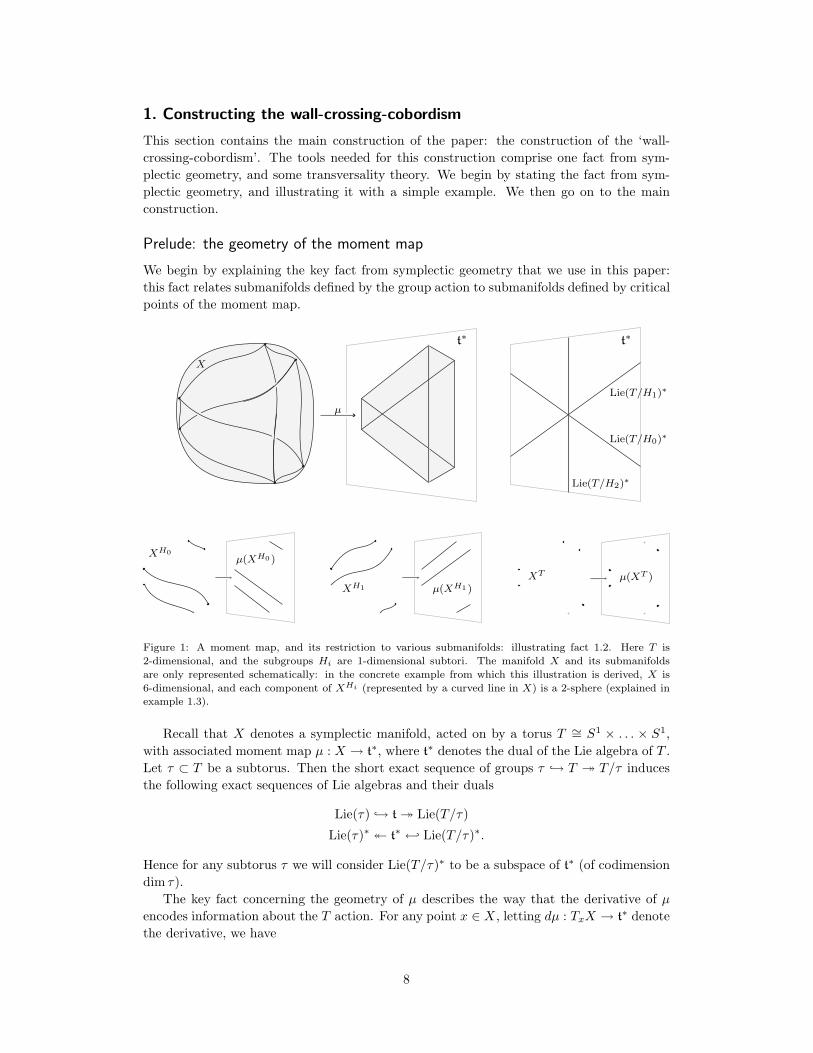
Definition 2.1. Associated to each transverse path Z ⊂ t∗ is a finite set data(Z), which we

refer to as the wall-crossing data for Z. We define data(Z) to be the set of pairs (H, q),

such that H ∼= S1 is an oriented subgroup of T , and q ∈ Z∩µ(XH). The orientation of H is

defined by the direction of the wall-crossing: we orient Z so that the positive direction goes

from p0 to p1; then a positive tangent vector in TqZ, thought of as an element of t∗, defines

a linear functional on t, and this restricts to a nonzero functional on h; and we orient H to

be positive with respect to this functional.

Remarks 2.2. 1. We may also apply the above definition to a closed 1-manifold Z ⊂ t∗,

as long as Z is oriented and transverse to µ. The wall-crossing data has a nontrivial

interpretation in this case, too.

2. We give an example to illustrate the orientation of H . Suppose our torus T is the

standard circle T = S1 = R/Z, with Lie algebra and its dual identified with R in the

standard manner. In this case p0 and p1 are real numbers. If p0 < p1, then Z must

be the interval [p0, p1], and each wall-crossing induces the positive (i.e. standard)

orientation on S1. If p1 < p0, then Z must be the interval [p1, p0], and each wall-

crossing induces the negative orientation on S1.)

3. It is not possible for the same pair (H, q) to appear twice in the wall-crossing data,

however we may have pairs (H0, q0) and (H1, q1) with H0 = H1 while q0 6= q1: since

Z may cross the same wall more than once; or Z may cross different walls which are

parallel and thus correspond to the same subgroup. And it is also possible for q0 to

equal q1 (with H0 6= H1). This is because a point q may lie in the interior of two

different walls simultaneously. This happens when components of the submanifolds

XH0 and XH1 are disjoint in X , while their images under µ both contain q0 = q1.

There are three points in figure 1 with this property.

12

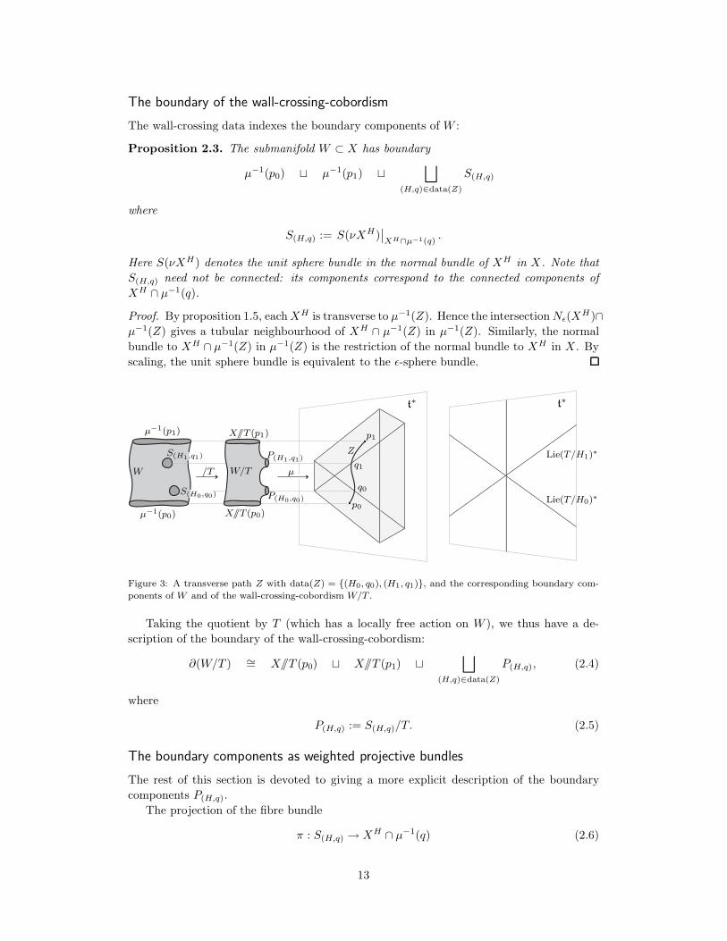
The boundary of the wall-crossing-cobordism

The wall-crossing data indexes the boundary components of W :

Proposition 2.3. The submanifold W ⊂ X has boundary

µ−1(p0) ⊔ µ−1(p1) ⊔⊔

(H,q)∈data(Z)

S(H,q)

where

S(H,q) := S(νXH)∣∣XH∩µ−1(q)

.

Here S(νXH) denotes the unit sphere bundle in the normal bundle of XH in X. Note that

S(H,q) need not be connected: its components correspond to the connected components of

XH ∩ µ−1(q).

Proof. By proposition 1.5, eachXH is transverse to µ−1(Z). Hence the intersectionNǫ(XH)∩

µ−1(Z) gives a tubular neighbourhood of XH ∩ µ−1(Z) in µ−1(Z). Similarly, the normal

bundle to XH ∩ µ−1(Z) in µ−1(Z) is the restriction of the normal bundle to XH in X . By

scaling, the unit sphere bundle is equivalent to the ǫ-sphere bundle.

µ−1(p0)

µ−1(p1)

X//T (p0)

X//T (p1)

p0

p1

q0

q1µ

Z

W /T W/T

S(H0,q0)

S(H1,q1)

P(H0,q0)

P(H1,q1)

Lie(T/H0)∗

Lie(T/H1)∗

t∗t∗

Figure 3: A transverse path Z with data(Z) = {(H0, q0), (H1, q1)}, and the corresponding boundary com-

ponents of W and of the wall-crossing-cobordism W/T .

Taking the quotient by T (which has a locally free action on W ), we thus have a de-

scription of the boundary of the wall-crossing-cobordism:

∂(W/T ) ∼= X//T (p0) ⊔ X//T (p1) ⊔⊔

(H,q)∈data(Z)

P(H,q), (2.4)

where

P(H,q) := S(H,q)/T. (2.5)

The boundary components as weighted projective bundles

The rest of this section is devoted to giving a more explicit description of the boundary

components P(H,q).

The projection of the fibre bundle

π : S(H,q) → XH ∩ µ−1(q) (2.6)

13

is a T -equivariant map, and by construction, T acts with at most finite stabilizers on the

total space S(H,q). The subgroup H acts trivially on the base, so that the T -action descends

to an action of T/H , and it follows from proposition 1.5 that this T/H-action on the base

is locally free.

We will first consider the quotient of the base of the fibre bundle (2.6), and then we will

state a proposition which describes the quotient of the total space.

The submanifold XH ⊂ X is a closed symplectic submanifold, stable under T , and the

restriction of the moment map µ to XH gives a moment map for the T -action on XH . Hence

the quotient of the base can be described as a symplectic quotient

(XH ∩ µ−1(q)

)/T = XH//T (q).

This looks like a singular kind of quotient: q is not a regular value of µ, for instance. But

the appearance of singularity is an illusion: we know a priori that H acts trivially on the

manifold XH , and so by Fact 1.2 we know that the image under µ of each component of

XH must lie in some affine hyperplane S ⊂ t∗ (parallel to Lie(T/H)∗). Now q is a regular

value in S for the restriction of µ, thought of as a map to S (the fact that q is a regular

value in this sense is equivalent to the condition that Z cross each wall in its interior).

Hence µ−1(q) ∩XH is a compact closed submanifold of XH , and its quotient XH//T (q) is

a compact symplectic orbifold. This kind of symplectic quotient is explained in more detail

in section 7.

Proposition 2.7. There exists a complex vector orbibundle

ν → XH//T (q)

together with an action of H on ν, covering the trivial action on X//T (q), and such that the

set of fixed points equals the zero section, such that

P(H,q)∼= S(ν)/H → XH//T (q).

Here S(ν) denotes the unit sphere bundle in ν (relative to a choice of invariant metric). In

the case that the symplectic quotient X//T (q) is a free quotient, ν is a vector bundle, induced

by the normal bundle νXH.

The vector bundle ν → X//T (q) is not uniquely defined: to defined it we choose a

complementary subgroup T ′ ⊂ T so that T = T ′ ×H . Then T ′ defines a lift of the action

of T/H on XH to its normal bundle νXH , and we let this action define the induced vector

orbibundle (as defined in appendix A) overXH//T (q). Then the H-action on νXH naturally

descends to an action on ν, and we will show that S(H,q)/T = S(ν)/H .

Proof of Proposition 2.7. The space S(H,q) is formed from νXH by the operations of taking

the sphere bundle, restriction, and taking the quotient by T . By decomposing T as T ′ ×H

we can take the quotient by T in two stages. The proof then amounts to permuting the

order of these operations (and seeing that the result is indepent of the order of operations).

Explicitly, S(H,q)/T =(S(νXH

∣∣XH∩µ−1(q)

)/T ′)/H = S(ν)/H.

The complex structure on ν is induced by fixing an invariant almost complex structure

on X , compatible with the symplectic form ω (see e.g. [25, Proposition 2.48]). It follows by

T -invariance that the normal bundle νXH is an invariant complex vector bundle, so that

the complex structure descends to the quotient ν.

14

Remarks 2.8. 1. In generalH will act on the fibres of ν with both positive and negative

weights (recall that H is oriented, and so has a natural identification with S1) and we

can thus decompose ν into the positive and negative weight subbundles ν = ν+ ⊕ ν−.

Letting ν− denote the same underlying real vector bundle as ν−, but with the con-

jugate complex structure (that is, with multiplication by i replaced by multiplication

by −i), then S(ν)/H can be identified with a weighted projectivization of ν+ ⊕ ν−.

Although this describes the diffeomorphism type of S(ν)/H , the natural orientation

of S(ν)/H (definition 3.5) is not given by this description.

2. The vector bundle ν depends on the choice of T ′. However the quotient S(ν)/H is

independent of this choice, as we can see from its description as S(H,q)/T . Changing

the choice of T ′ has the effect of tensoring ν with a certain line bundle, but this

change doesn’t affect the quotient S(ν)/H . This can be seen as a generalization of

the fact that the projectivization of a complex vector bundle bundle is invariant under

tensoring the vector bundle with a line bundle.

3. The orbifold singularities and orientation of the wall-crossing-cobordism

Orbifold singularities in the wall-crossing-cobordism

We now address the question of the orbifold singularities in the wall-crossing-cobordism

W/T . These arise from points in W whose stabilizer subgroup is nontrivial. To be more

precise, since we allow for the possibility that there is some finite subgroup of T which

stabilizes every point in X , the orbifold singularities arise from points in W whose stabilizer

subgroup is larger than the generic one.

Lemma 3.1. Let F ⊂ T be a finite subgroup, and XF ⊂ X the subset of points fixed by

F . Then XF is a closed symplectic submanifold of X, transverse to ∂W , and also to the

interior of W . It follows that the wall-crossing-cobordism W/T is an orbifold-with-boundary.

This lemma gives both coarse information, and very fine information. The coarse in-

formation provided by this lemma is that the wall-crossing-cobordism is an orbifold-with-

boundary, which we will see is oriented, and hence satisfies Stokes’s theorem.

However, this lemma actually makes it possible to determine the structure of the orbifold

singularities quite accurately. This is because each XF is a closed symplectic submanifold

of X , and it follows that the restriction of the moment map µ to XF gives a moment map

for the action of T on XF , where the walls and chambers of the image of µ for XF being a

subset of the corresponding walls and chambers for X . Thus we can treat all the arguments

in this paper as applying simultaneously to X and to XF : each symplectic quotient X//T (p)

contains the symplectic quotient XF //T (p), as does each wall-crossing-cobordism, and so

on. (We won’t have cause to carry out such a detailed analysis in this paper.)

Proof of lemma 3.1. The fact that XF is a closed manifold is a standard result of the theory

of compact group actions on manifolds (proved using an equivariant exponential map, see

e.g. [5]), and an easy averaging argument shows that the restriction of the symplectic form

ω to XF is nondegenerate.

Now, let X∗ ⊂ X denote the set of points with finite stabilizer subgroup. Then W ⊂ X∗,

by construction. Any p ∈ t∗ is a regular value for µ|X∗ , and using the same argument as in

the proof of Proposition 1.5 we see that µ−1(p) ∩X∗ is transverse to XF . It follows XF is

transverse to W , and to the boundary components µ−1(p0) and µ−1(p1).

15

It remains to show transversality to the boundary components S(H,q). The description

of S(H,q) as the sphere bundle in a vector bundle makes it clear that the stabilizer doesn’t

depend on the radius of the sphere.

By varying the radius of the sphere, we can foliate W locally by a one-parameter family

of submanifolds. Since XF is transverse to W , to show transversality to one of the leaves of

this foliation, we must simply show that for every point in the intersection with XF , there

is a tangent vector to XF which is transverse to the leaves of the foliation. But this follows

from the fact that the stabilizer subgroup is independent of the radius of the sphere.

Orienting the wall-crossing-cobordism

In this subsection we define an orientation on the wall-crossing-cobordism W/T . We then

calculate the induced orientations on its various boundary components.

Definition 3.2. The orientation is extremely easy from a conceptual point of view: W/T

is foliated by symplectic orbifolds X//T (p)∩W/T , for p ∈ Z, and the normal bundle to this

foliation is identified with TZ by the moment map. Thus the symplectic orientation of the

leaves, combined with the orientation of Z in which the positive direction goves from p0 to

p1, gives an orientation of the wall-crossing-cobordism W/T .

To carry this out explicitly, we begin by fixing a metric on W/T . Let x be a point in W ,

denote by [x] the corresponding point in W/T , and set p = µ(x). We assume for simplicity

that [x] is a smooth point of W/T (but by using orbifold metrics and orbifold differential

forms, as described in appendix A, this construction also works at the orbifold points). By

construction, dµ is surjective at x (fact 1.1). Moreover, since µ is T -invariant, it descends

to a map from W/T to Z. We can thus decompose the tangent space T[x](W/T ) into the

kernel and the cokernel of dµ. Identifying these spaces explicitly gives us

T[x](W/T ) ∼= T[x]X//T (p)⊕ TpZ.

Now X//T (p) is a symplectic orbifold, and we denote its symplectic form by ωp. Using the

above decomposition, we can extend ωp to T[x](W/T ). denoting the extension by ωp (this

2-form will not necessarily be closed, but it will be nondegenerate on the tangent spaces to

the leaves). Let Z be parametrized by the variable t, with t = 0 at p0 and t = 1 at p1. Then

ωkp ∧ µ∗dt

(where dimX//T (p) = 2k) defines a top-degree form, and hence an orientation of W/T at

[x]. But the above construction can be simultaneously applied to every smooth point of

W/T , with the resulting form varying smoothly, hence orienting W/T .

Remark 3.3. In fact, the above definition can be enhanced in a straighforward manner to

define a ‘complex orientation’ of W/T . We won’t need it in this paper, however.

The rest of this section is taken up with describing in a precise way an orientation on the

wall-crossing boundary components ofW/T , and then stating the result that this orientation

equals the induced boundary orientation. We give two definitions, and then state this result

(the proof of which is given in appendix C).

Definition 3.4. Let V be an oriented real vector space, and suppose the oriented group

H ∼= S1 acts on V , fixing only the origin. We define the induced orientation of S(V )/H

16

(where S(V ) denotes the unit sphere in V relative to an invariant metric). Given a point

v ∈ S(V ), denote byH ·v ∈ S(V )/H the associatedH-orbit. There is a natural isomorphism

TH·v(S(V )/H)⊕ R+ · v ⊕ h ∼= TvV ∼= V,

where R+ ·v denotes the ray from the origin through v. We define the orientation of S(V )/H

to be that orientation which is compatible with the above isomorphism together with the

given orientations of R+, h, and V .

For example, let V = Cn, and let H ∼= S1 act with weight 1. Then S(V )/H is naturally

identified with complex projective space, and the orientation we have defined agrees with

the orientation induced by the complex structure. Similarly, if H acts with positive weights,

then S(V )/H is a weighted projective space, and the above-defined orientation again agrees

with the orientation induced by the complex structure (see appendix B for more details).

We now define an orientation on the boundary components of the wall-crossing-cobordism

corresponding to wall-crossings. We then prove that this agrees with the induced boundary

orientation.

Definition 3.5. Recall that proposition 2.7 identifies the boundary component of the wall-

crossing-cobordism corresponding to the pair (H, q) as the total space of the bundle

S(H,q)/T = S(ν)/H → XH//T (q).

where ν → XH//T (q) is a vector bundle induced by the normal bundle νXH and a decompos-

tion of T as T ′×H . We orient this space as follows. Since XH is a symplectic submanifold,

the symplectic orientations of X and of XH induce a natural orientation on the normal

bundle νXH , which descends (by invariance) to the induced bundle V . Combining this

with definition 3.4 and the orientation of H given in definition 2.1 gives an orientation of

the fibres of the bundle S(ν)/H → XH//T (q). The base is a symplectic quotient, and we

orient it by its symplectic form. We then orient the total space S(ν)/H by the product

orientation. (the order is irrelevant, since both the base and fibre are even-dimensional).

Lemma 3.6. Let the wall-crossing-cobordism W/T be oriented as in definition 3.2. Then

the induced boundary orientation of X//T (p0) is −(ωkp0), and of X//T (p1) is ωkp1 (where ωpi

denote the respective induced symplectic forms), and the induced boundary orientation of

each P(H,q) is equal to the product orientation defined in 3.5 above.

The proof is conceptually rather simple, but keeping track of the various vector spaces

involved in a comprehensible way makes it quite long, and it has been relegated to ap-

pendix C.

4. Theorem A: a summary of the existence and properties of the wall-

crossing-cobordism.

Theorem A. Suppose p0, p1 ∈ t∗ are regular values of the moment map µ, and let Z ⊂ t∗

be path joining p0 and p1 which is transverse to µ. There there are two objects naturally

associated to Z. The first is a finite set data(Z), consisting of pairs (H, q), where H ∼= S1

is a subgroup of T , and q is a point in t∗. And the second object naturally associated to Z

is an oriented cobordism, whose boundary equals

−X//T (p0) ⊔ X//T (p1) ⊔⊔

(H,q)∈data(Z)

P(H,q).

For each pair (H, q) ∈ data(Z) the space P(H,q) is the total space of a bundle over the

compact symplectic orbifold XH//T (q), whose fibres are weighted projective spaces.

17

Moreover

1. The cobordism arises as the quotient, by T , of a submanifold-with-boundary W ⊂ X ,

such that the T -action on W is locally free.

2. The points p0 and p1 need not lie in the image of µ. If either lies outside the image of

µ, then the associated boundary component is empty.

3. The boundary component −X//T (p0) denotes X//T (p0) with the negative of its sym-

plectic orientation.

4. Each space P(H,q) can be described as follows. There exists a complex vector orbibun-

dle ν → XH//T (q), with an action of H on the fibres, such that

P(H,q) = S(ν)/H → XH//T (q).

The bundle ν → XH//T (q) is induced by the normal bundle νXH , and depends on

the choice of a complement to H in T ; however the bundle P(H,q) → XH//T (q) is

independent of this choice.

5. The induced orientations on the spaces P(H,q) are given by the product of the symplec-

tic orientation of XH//T (q) and a natural orientation on the fibres, defined in terms

of the oriented group H , and the oriented fibres of ν.

6. The wall-crossing-data data(Z) is determined by the arrangement of walls in t∗ (which

can be deduced from the fixed point data of (X,T, µ)), together with the path Z.

5. The localization map and the wall-crossing formula

In this section we fix our attention on a single wall-crossing. Fixing notation, we suppose

p0, p1 ∈ t∗ are regular values of µ, joined by a transverse path Z having a single wall-crossing

at q, and we let H ∼= S1 be the oriented subgroup associated to the wall.

Theorem A says, roughly, that the symplectic quotients X//T (p0) and X//T (p1) are in

some way related by the symplectic quotient XH//T (q). Theorem B gives a cohomologically

precise version of this.

Theorem B. There is a map

λH : H∗T (X)→ H∗

T/H(XH)

such that, for any a ∈ H∗T (X),

∫

X//T (p0)

κ(a)−

∫

X//T (p1)

κ(a) =

∫

XH//T (q)

κ(λH(a|XH )).

(The maps κ on the left hand side are the natural maps H∗T (X)→ H∗(X//T (pi)) and on the

right hand side is the natural map H∗T/H(XH)→ H∗(XH//T (q)).)

Moreover, for any component XHi ⊂ XH, the restriction of λH(a) to XH

i only depends

on the restriction of a to XHi .

Recall that XH//T (q) can be considered to be a symplectic quotient of XH by the

quotient group T/H (expained in section 2); and the various maps denoted by κ are defined

by restriction to the relevant submanifold, followed by the natural identification of the

equivariant cohomology of this manifold with the rational cohomology of its quotient.

18

We call λH the localization map: we first define λH , and then we prove theorem B.

In the next section we give an explicit formula for λH in terms of characteristic classes.

The localization map is the key to an inductive process, which will allow us to localize

calculations to the fixed points XT . We will carry out the induction in section 8.

Definition 5.1. The localization map λ depends on the triple (X,T,H), where X is a

symplectic manifold, T is a compact torus which acts on X (preserving the symplectic

form), and H ∼= S1 is an oriented subgroup of T . In this section, X and T will be fixed, and

we will write λH to denote the dependence on the oriented subgroup H (in later sections

will decorate the symbol λ with any data that is not obvious from the context.)

Given X and T , then λH is the (degree-lowering) map

λH : H∗T (X)→ H∗

T/H(XH)

defined as follows. Let S(νXH) denote the sphere bundle in the normal bundle νXH to XH

in X . We then denote by p and π the projections

S(νXH)/H //

p$$III

IIIIII

S(νXH)/H

πyyssssssssss

XH

Let π∗ denote integration over the fibres of π (where the fibres are oriented according the

definition 3.4, using the symplectic orientation of the normal bundle to XH). Then we let

λH equal the composition

H∗T (S(νXH))

/H

∼=// H∗T/H(S(νXH)/H)

π∗

��H∗T (X)

i∗ // H∗T (XH)

p∗

OO

H∗T/H(XH)

where i : XH → X denotes the inclusion, and the map H∗T (S(νXH))

/H−−→∼=

H∗T/H(S(νXH)/H)

is the natural map on equivariant cohomology induced by the locally free quotient (see for

example [1]).

Proof of theorem B. The proof is a straightforward exercise involving identifying the various

maps involved, and repeatedly using the fact that integration over the fibre commutes with

restriction (together with some general facts about equivariant cohomology.)

Let j : W → X denote the inclusion. Then, for any a ∈ H∗T (X), we have j∗(a) ∈ H∗

T (W ),

and we write

j∗(a)/T ∈ H∗(W/T ),

for the corresponding naturally induced class (recall that the T -action is locally free on W ,

and we are taking cohomology with rational coefficients).

Since the wall-crossing-cobordism W/T is an oriented orbifold-with-boundary, it follows

that the boundary is homologous to zero (fact A.5), and hence

∫

∂(W/T )

j∗(a)/T = 0.

19

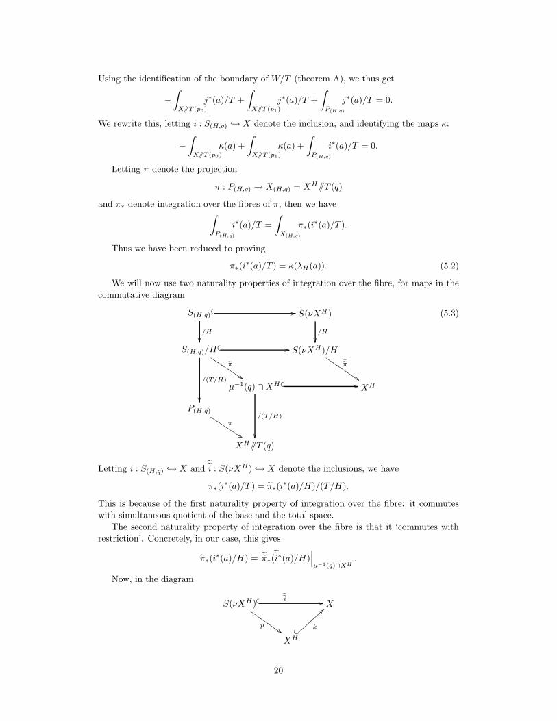
Using the identification of the boundary of W/T (theorem A), we thus get

−

∫

X//T (p0)

j∗(a)/T +

∫

X//T (p1)

j∗(a)/T +

∫

P(H,q)

j∗(a)/T = 0.

We rewrite this, letting i : S(H,q) → X denote the inclusion, and identifying the maps κ:

−

∫

X//T (p0)

κ(a) +

∫

X//T (p1)

κ(a) +

∫

P(H,q)

i∗(a)/T = 0.

Letting π denote the projection

π : P(H,q) → X(H,q) = XH//T (q)

and π∗ denote integration over the fibres of π, then we have∫

P(H,q)

i∗(a)/T =

∫

X(H,q)

π∗(i∗(a)/T ).

Thus we have been reduced to proving

π∗(i∗(a)/T ) = κ(λH(a)). (5.2)

We will now use two naturality properties of integration over the fibre, for maps in the

commutative diagram

S(H,q)�

� //

/H

��

S(νXH)

/H

��S(H,q)/H

�

� //

/(T/H)

��

π

$$JJJJJJJJJS(νXH)/H

˜π

$$IIIIIIIII

µ−1(q) ∩XH �

� //

/(T/H)

��

XH

P(H,q)

π

%%JJJJJJJJJ

XH//T (q)

(5.3)

Letting i : S(H,q) → X and˜i : S(νXH) → X denote the inclusions, we have

π∗(i∗(a)/T ) = π∗(i

∗(a)/H)/(T/H).

This is because of the first naturality property of integration over the fibre: it commutes

with simultaneous quotient of the base and the total space.

The second naturality property of integration over the fibre is that it ‘commutes with

restriction’. Concretely, in our case, this gives

π∗(i∗(a)/H) = ˜π∗ (i

∗(a)/H)∣∣∣µ−1(q)∩XH

.

Now, in the diagram

S(νXH)�

�

˜i //

p$$II

IIIII

IIX

XH.

�

k

>>}}}}}}}}

20

an easy scaling argument shows that˜i is equivariantly homotopic to k ◦ p. Hence

˜π∗ (i∗(a)/H) = ˜π∗(p

∗(k∗(a))/H)

= λH(a)

since this turns out to be precisely the definition of λH , with the data (X,T,H).

Putting all this together, we thus have

π∗(i∗(a)/T ) =

(λH(a)|µ−1(q)∩XH

)/(T/H)

= κ(λH(a))

by definition of κ. But this proves equation (5.2), and hence, by the arguments preceding

equation (5.2), we have completed the proof.

6. The wall-crossing formula in terms of characteristic classes

By giving an explicit formula for the localization map in terms of characteristic classes, we

can restate a more explicit version of the wall-crossing formula (which we call theorem B′.)

We can give an explicit formula for the localization map λH using the definitions and

results of appendix B. Using this explicit formula, we can then recast theorem B in a

more explicit form. Before carrying this out, we must give a definition, which will help us

account for the possibility that XH has a number of components, and describe the way a

decomposition of T induces a decomposition of a cohomology class.

Definition 6.1. Let Y be a connected manifold with an action of T . We define oT (Y ) to

be the order of the maximal subgroup of T which stabilizes every point in Y (so oT (Y ) = 1

if and only if T acts effectively on Y ). (In every case which we consider, this number will be

finite). We extend this definition to the case in which Y may have a number of components

by defining oT (Y ) to be the degree-0 cohomology class which restricts to give this number

on each component.

Now suppose T ′ ⊂ T is a complement to H , so that T = T ′ ×H . Then the restriction

of any class a ∈ H∗T (X) to XH decomposes

a|XH =∑

i≥0

ai ⊗ ui (6.2)

according to the natural isomorphism

H∗T (XH) ∼= H∗

T ′(XH)⊗H∗(BH),

where u ∈ H2(BH) is the positive generator (with respect to the orientation of H defined

in 2.1).

We then have

Proposition 6.3. Let a ∈ H∗T (X), and suppose T ′ ⊂ T is a complement to H, so that

T = T ′ ×H. Then

λH(a) =oT (X)

oT/H(XH)

∑

i≥0

ai ⌣ swi−r+1,

where the classes ai ∈ H∗T ′(XH) are defined by the natural decomposition of a given in equa-

tion (6.2) above, and swi denotes the i-th T ′-equivariant weighted Segre class of (νXH , H)

(definitions B.6 and B.12), and r is the function, constant on connected components of XH,

such that 2r = rk(νXH).

21

Proof. We will show how this proposition follows from the integration formula proved in

appendix B, namely proposition B.8 (together with its ‘equivariant enhancement’, equation

(B.14)).

Explicitly, we are using the vector bundle νXH → XH and the groups H and T ′ in place

of the vector bundle V → Y and the groups S1 and G in appendix B.

We need first to give the normal bundle νXH a complex structure compatible with its

symplectic form, so that the definition of the orientation of S(νXH)/H used in appendix B

agrees with its natural orientation (definition 3.5). And second, we must show that our factor

oT (X)/oT/H(XH) is equal, on each component of XH , to the factor k in the appendix.

Firstly, general principles in symplectic topology imply that there exists a T -invariant

almost complex structure J : TX → TX , compatible with the symplectic form ω, and such

that TXH is stable under J (see, for example, McDuff and Salamon [25, Proposition 2.48]).

Such an almost complex structure gives the normal bundle νXH a complex structure, and

the orientations induced by the complex structure and the symplectic form agree (equation

(0.3)), and thus we can apply Proposition B.8 with this complex structure.

Secondly, we need to show that, for each component XHi of XH , we have

k = oT (X)/oT/H(XHi ),

where k is the greatest common divisor of the weights of the H-action on the fibres of

νXHi → XH

i . But using the decomposition T = T ′×H , together with lemma 3.1, it is clear

that k = oH(νXHi ), and that oT (X) = oT ′×H(νXH

i ) = oT ′(XHi ) · oH(νXH

i ).

We can now rewrite theorem B using this explicit identification.

Theorem B′. Suppose p0, p1 ∈ t∗ are regular values of µ, joined by a transverse path Z

which has a single wall-crossing, at q. Let H ∼= S1 be the subgroup associated to the wall,

and choose T ′ ⊂ T so that T = T ′ ×H.

Then there are characteristic classes swi ∈ H2iT ′(XH) (the equivariant weighted Segre

classes of νXH , as defined in B.6) such that, for any a ∈ H∗T (X),

∫

X//T (p0)

κ(a)−

∫

X//T (p1)

κ(a) =

∫

XH//T ′(q)

κ

(oT (X)

oT/H(XH)

∑i≥0 ai ⌣ swi−r+1

).

where r is the function, constant on connected components of XH, such that 2r = rk(νXH);

and the classes ai ∈ H∗T ′(XH) are defined by restricting a to XH and decomposing, as in

equation (6.2) above. (The map κ on the left hand side of the main equation is the natural

map H∗T (X)→ H∗(X//T (pi)) and on the right hand side is the natural map

H∗T ′(XH)→ H∗(XH//T ′(q)).)

7. A generalization of a transverse path and its data

This is the first of three sections in which we apply the preceding results inductively, ending

up with results concerning the T -fixed points of X . In this section we generalize the notion

of a transverse path, and the associated data. In section 8 we show how this generalized

data corresponds to cobordisms involving the fixed points XT , and in section 9 we show

how this generalized data governs integration formulae localized at the fixed points.

A τ -transverse path and its data

We begin with a straightforward generalization of the notion of a transverse path, and its

associated data. Recall that X is a symplectic manifold, with an action of the torus T , and

22

with associated moment map µ : X → t∗. Let τ ⊂ T be a subtorus. In section 1 we saw

how Lie(T/τ)∗ can be considered to be a subspace of t∗ via a natural embedding (it is a

subspace of dimension dimT − dim τ). Recall also that Xτ , the set of points fixed by τ , is

a closed symplectic submanifold of X .

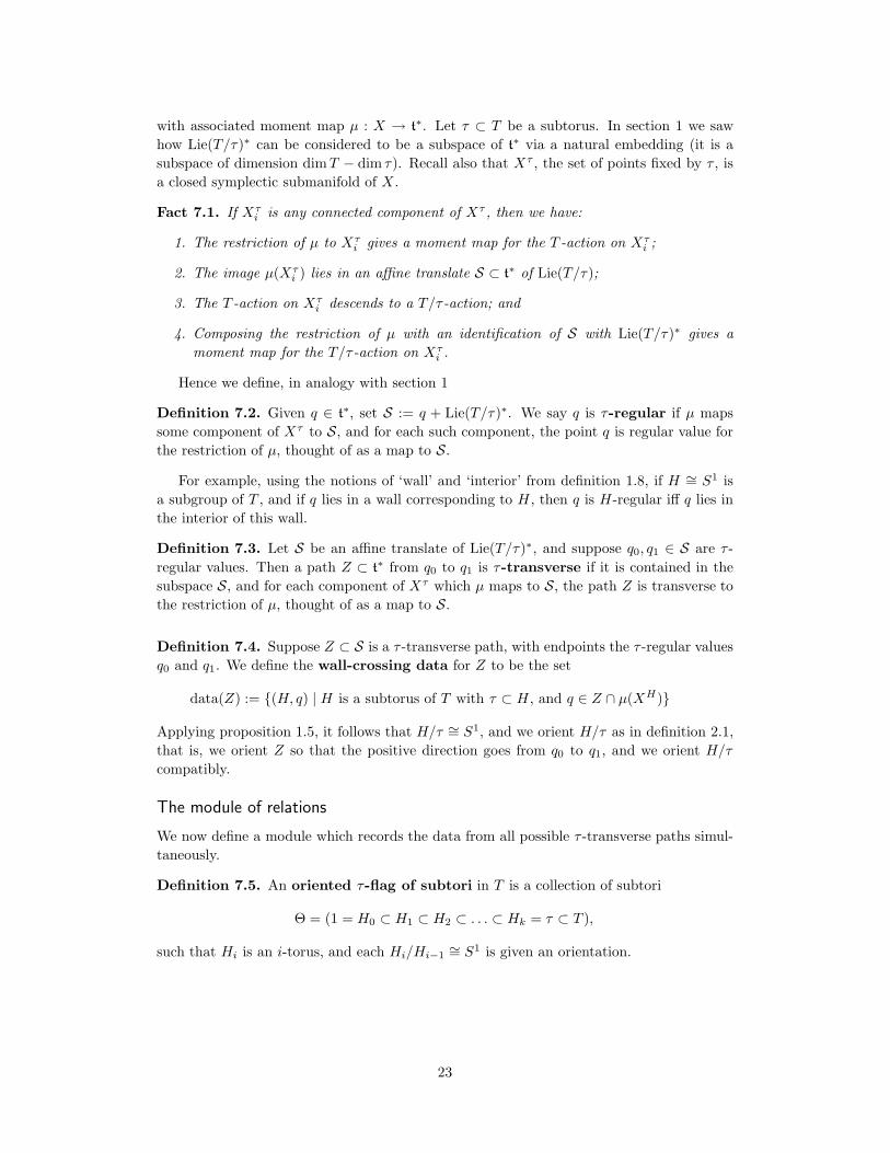
Fact 7.1. If Xτi is any connected component of Xτ , then we have:

1. The restriction of µ to Xτi gives a moment map for the T -action on Xτ

i ;

2. The image µ(Xτi ) lies in an affine translate S ⊂ t∗ of Lie(T/τ);

3. The T -action on Xτi descends to a T/τ-action; and

4. Composing the restriction of µ with an identification of S with Lie(T/τ)∗ gives a

moment map for the T/τ-action on Xτi .

Hence we define, in analogy with section 1

Definition 7.2. Given q ∈ t∗, set S := q + Lie(T/τ)∗. We say q is τ-regular if µ maps

some component of Xτ to S, and for each such component, the point q is regular value for

the restriction of µ, thought of as a map to S.

For example, using the notions of ‘wall’ and ‘interior’ from definition 1.8, if H ∼= S1 is

a subgroup of T , and if q lies in a wall corresponding to H , then q is H-regular iff q lies in

the interior of this wall.

Definition 7.3. Let S be an affine translate of Lie(T/τ)∗, and suppose q0, q1 ∈ S are τ -

regular values. Then a path Z ⊂ t∗ from q0 to q1 is τ-transverse if it is contained in the

subspace S, and for each component of Xτ which µ maps to S, the path Z is transverse to

the restriction of µ, thought of as a map to S.

Definition 7.4. Suppose Z ⊂ S is a τ -transverse path, with endpoints the τ -regular values

q0 and q1. We define the wall-crossing data for Z to be the set

data(Z) := {(H, q) | H is a subtorus of T with τ ⊂ H , and q ∈ Z ∩ µ(XH)}

Applying proposition 1.5, it follows that H/τ ∼= S1, and we orient H/τ as in definition 2.1,

that is, we orient Z so that the positive direction goes from q0 to q1, and we orient H/τ

compatibly.

The module of relations

We now define a module which records the data from all possible τ -transverse paths simul-

taneously.

Definition 7.5. An oriented τ-flag of subtori in T is a collection of subtori

Θ = (1 = H0 ⊂ H1 ⊂ H2 ⊂ . . . ⊂ Hk = τ ⊂ T ),

such that Hi is an i-torus, and each Hi/Hi−1∼= S1 is given an orientation.

23

Definition 7.6. We define the Z-module A by

A :=⊕

τ⊂T

Aτ ,

as τ runs through all subtori of T , where

Aτ :=⊕

Z(Θ, q)

is the set of formal linear combinations of pairs (Θ, q), where q is τ -regular and Θ is an

oriented τ -flag of subtori.

Note that Aτ will be nontrivial for only finitely many τ , namely those for which there

exists a τ -regular value. These correspond to the τ such that there is some point x ∈ X

whose stabilizer subgroup has identity component τ (the fact that there are only finitely

many such τ is a standard fact in the theory of group actions on manifolds [5, 19]). We also

note that AT corresponds to the T -fixed points of X : if (Θ, q) ∈ AT then q ∈ t∗ is one of

the finite set of points in the set µ(XT ) ⊂ t∗.

Definition 7.7. We now define the submodule of relations R ⊂ A. There are two kinds of

generators of R. The first kind comes from a pair consisting of a τ -transverse path Z and

an oriented τ -flag of subtori Θ, for any choice of subtorus τ . The associated generator of R

is the sum

−(Θ, q0) + (Θ, q1) +∑

(H,r)∈data(Z)

(Θ ∪H, r),

where q0 and q1 are the endpoints of Z, and Θ ∪H denotes the oriented H-flag defined by

concatenating Θ and H , with H/τ oriented as in data(Z). The second kind of generator of

R corresponds to points which are outside the image of µ: for any subtorus τ ⊂ T , suppose

q is a τ -regular value and let Θ be an oriented τ -flag. If q /∈ µ(Xτ ) then

(Θ, q)

is a generator of R. Finally, given (Θ, q) ∈ A, we write [Θ, q] for its equivalence class in the

quotient module A/R.

Since X is compact, for any regular value p0 ∈ t∗, there is a path Z starting at p0

and ending outside the image of the moment map. The corresponding fact is true for each

Xτ ⊂ X . Hence

Lemma 7.8. For any (Θ, q) ∈ A we have

[Θ, q] =∑

i∈I

[Θi, vi]

in A/R, where I is a finite indexing set, and each (Θi, vi) ∈ AT .

8. Cobordisms between symplectic quotients and bundles over the fixed

points

In this section we show how the relations defined in the previous section correspond to

cobordisms. We begin by defining, for each generator (Θ, q) of A, a space P(Θ,q). We will

then show how ‘relations’, i.e. finite sums in the submodule R, correspond to cobordisms

between these spaces. The constructions in this section are illustrated in figure 8.

24

The spaces involved

For every pair (Θ, q), where Θ is a τ -flag and q ∈ t∗ is a τ -regular value, we will define

an associated space P(Θ,q). We first describe P(Θ,q) in two special cases, and then give the

general definition. In the case that τ = {1} is the trivial group, then the only τ -flag is the

trivial flag, which we denote by 1 ⊂ T , and a τ -regular value is just a regular value of the

moment map µ : X → t∗. In this case

P(1⊂T,q) = X//T (q).

If Z ⊂ t∗ is a transverse path, and (H, q) ∈ data(Z) is one of its wall-crossing pairs, then it

follows that q is an H-regular value, and H ∼= S1 defines the oriented H-flag 1 ⊂ H ⊂ T ,

and we have

P(1⊂H⊂T,q) = P(H,q),

where the space on the right is the wall-crossing space defined in equation (2.5).

Definition 8.1. Suppose the torus τ acts on the complex vector space V , with 0 ∈ V the

only point fixed by τ . Then associated to every flag of subtori of τ is a submanifold of

V on which the τ -action is locally free (this submanifold may be empty). To define the

submanifold, we first define a canonical decomposition of V . Let Θ = (1 = H0 ⊂ H1 ⊂

. . . ⊂ Hk = τ) be a τ -flag, that is, a full flag of subtori of τ . There is an associated flag of

subspaces of V , stable under the τ -action:

V = V H0 ⊃ V H1 ⊃ . . . ⊃ V Hk = {0}

where V Hi is the subspace fixed by Hi. We define Vi ⊂ V to be the orthogonal complement

to V Hi in V Hi−1 , relative to a τ -invariant metric, for 1 ≤ i ≤ k. Then Vi ∼= V Hi−1/V Hi ,

and these subspaces define a decomposition of V into subrepresentations

V = V1 ⊕ V2 ⊕ . . .⊕ Vk.

We set

SΘ(V ) := S(V1)× S(V2)× . . .× S(Vk) ⊂ V

where S(Vi) is the unit sphere, relative to an invariant metric. Note that SΘ(V ) will be

nonempty precisely when each Vi is nontrivial, that is, when each inclusion is strict in the

flag of subspaces V H0 ⊃ V H1 ⊃ . . . ⊃ V Hk .

Finally, we define

PΘ(V ) := SΘ(V )/τ.

This is a locally free quotient, and hence has the structure of an orbifold. An orientation

of V induces an orientation on PΘ(V ) as follows. We fix an orientation of each Vi so that

the product orientation equals the given orientation of V . We then orient each S(Vi)/Ti by

applying the formula of definition 3.4, and give PΘ(V ) the induced product orientation (see

the end of this section, where the structure of PΘ(V ) is described in more detail).

Remarks 8.2. 1. To see that the τ -action is locally free on SΘ(V ) we choose a decom-

position of τ which is compatible with Θ, that is

τ = T1 × T2 × . . .× Tk,

where each Ti ∼= Hi/Hi−1∼= S1. Then the above decomposition of V has the property

that the Ti-action on Vi leaves only 0 ∈ Vi fixed, so that the Ti-action on S(Vi) is

locally free.

25

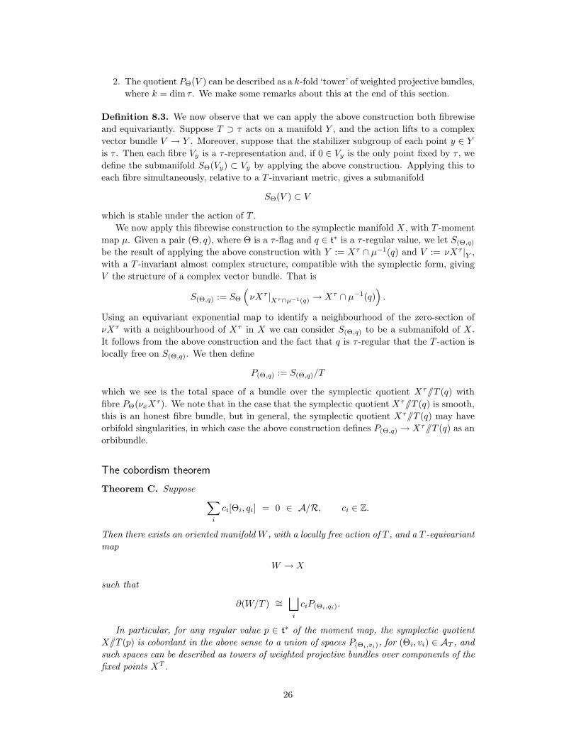
2. The quotient PΘ(V ) can be described as a k-fold ‘tower’ of weighted projective bundles,

where k = dim τ . We make some remarks about this at the end of this section.

Definition 8.3. We now observe that we can apply the above construction both fibrewise

and equivariantly. Suppose T ⊃ τ acts on a manifold Y , and the action lifts to a complex

vector bundle V → Y . Moreover, suppose that the stabilizer subgroup of each point y ∈ Y

is τ . Then each fibre Vy is a τ -representation and, if 0 ∈ Vy is the only point fixed by τ , we

define the submanifold SΘ(Vy) ⊂ Vy by applying the above construction. Applying this to

each fibre simultaneously, relative to a T -invariant metric, gives a submanifold

SΘ(V ) ⊂ V

which is stable under the action of T .

We now apply this fibrewise construction to the symplectic manifold X , with T -moment

map µ. Given a pair (Θ, q), where Θ is a τ -flag and q ∈ t∗ is a τ -regular value, we let S(Θ,q)

be the result of applying the above construction with Y := Xτ ∩ µ−1(q) and V := νXτ |Y ,

with a T -invariant almost complex structure, compatible with the symplectic form, giving

V the structure of a complex vector bundle. That is

S(Θ,q) := SΘ

(νXτ |Xτ∩µ−1(q) → Xτ ∩ µ−1(q)

).

Using an equivariant exponential map to identify a neighbourhood of the zero-section of

νXτ with a neighbourhood of Xτ in X we can consider S(Θ,q) to be a submanifold of X .

It follows from the above construction and the fact that q is τ -regular that the T -action is

locally free on S(Θ,q). We then define

P(Θ,q) := S(Θ,q)/T

which we see is the total space of a bundle over the symplectic quotient Xτ//T (q) with

fibre PΘ(νxXτ). We note that in the case that the symplectic quotient Xτ//T (q) is smooth,

this is an honest fibre bundle, but in general, the symplectic quotient Xτ//T (q) may have

orbifold singularities, in which case the above construction defines P(Θ,q) → Xτ//T (q) as an

orbibundle.

The cobordism theorem

Theorem C. Suppose∑

i

ci[Θi, qi] = 0 ∈ A/R, ci ∈ Z.

Then there exists an oriented manifold W , with a locally free action of T , and a T -equivariant

map

W → X

such that

∂(W/T ) ∼=⊔

i

ciP(Θi,qi).

In particular, for any regular value p ∈ t∗ of the moment map, the symplectic quotient

X//T (p) is cobordant in the above sense to a union of spaces P(Θi,vi), for (Θi, vi) ∈ AT , and

such spaces can be described as towers of weighted projective bundles over components of the

fixed points XT .

26

µ−1(p0)

µ−1(p1)

p0

p1

q0

q1µ

X

ZW

Z0

Z1

q2

q3

r0

r1

S0

S1

Lie(T/τ0)∗

Lie(T/τ1)∗

t∗t∗

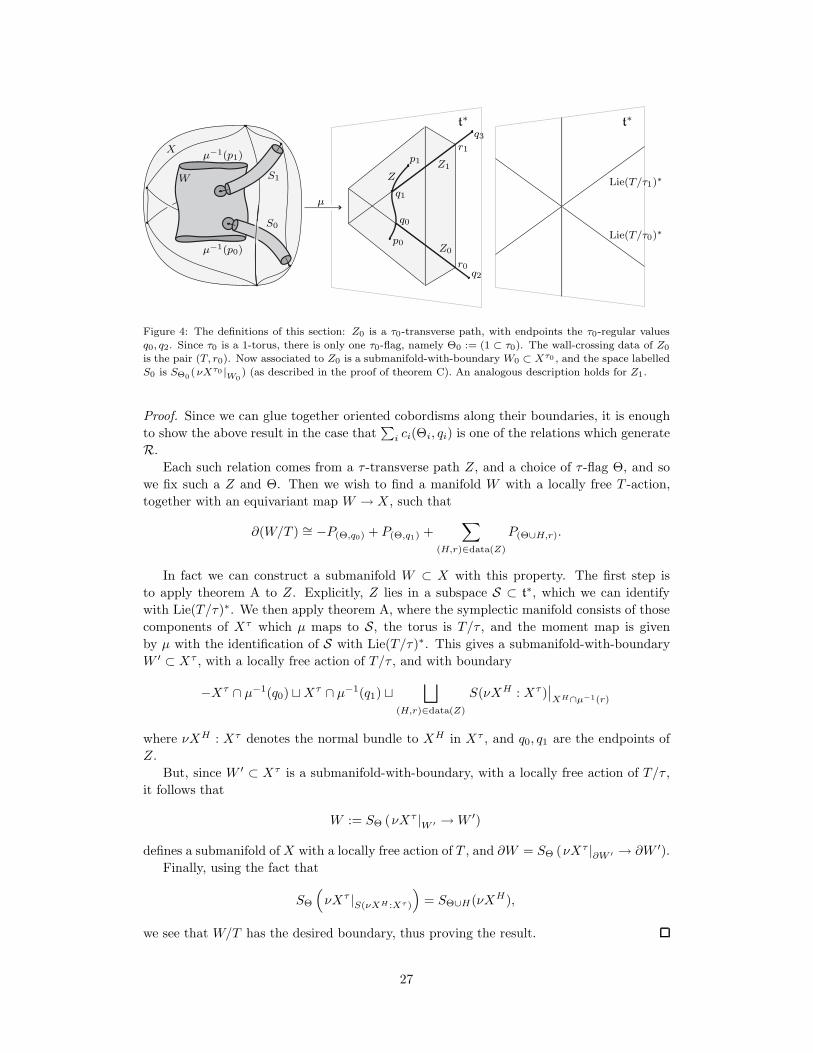
Figure 4: The definitions of this section: Z0 is a τ0-transverse path, with endpoints the τ0-regular values

q0, q2. Since τ0 is a 1-torus, there is only one τ0-flag, namely Θ0 := (1 ⊂ τ0). The wall-crossing data of Z0

is the pair (T, r0). Now associated to Z0 is a submanifold-with-boundary W0 ⊂ Xτ0 , and the space labelled

S0 is SΘ0(νXτ0 |W0

) (as described in the proof of theorem C). An analogous description holds for Z1.

Proof. Since we can glue together oriented cobordisms along their boundaries, it is enough

to show the above result in the case that∑

i ci(Θi, qi) is one of the relations which generate

R.

Each such relation comes from a τ -transverse path Z, and a choice of τ -flag Θ, and so

we fix such a Z and Θ. Then we wish to find a manifold W with a locally free T -action,

together with an equivariant map W → X , such that

∂(W/T ) ∼= −P(Θ,q0) + P(Θ,q1) +∑

(H,r)∈data(Z)

P(Θ∪H,r).

In fact we can construct a submanifold W ⊂ X with this property. The first step is

to apply theorem A to Z. Explicitly, Z lies in a subspace S ⊂ t∗, which we can identify

with Lie(T/τ)∗. We then apply theorem A, where the symplectic manifold consists of those

components of Xτ which µ maps to S, the torus is T/τ , and the moment map is given

by µ with the identification of S with Lie(T/τ)∗. This gives a submanifold-with-boundary

W ′ ⊂ Xτ , with a locally free action of T/τ , and with boundary

−Xτ ∩ µ−1(q0) ⊔Xτ ∩ µ−1(q1) ⊔

⊔

(H,r)∈data(Z)

S(νXH : Xτ )∣∣XH∩µ−1(r)

where νXH : Xτ denotes the normal bundle to XH in Xτ , and q0, q1 are the endpoints of

Z.

But, since W ′ ⊂ Xτ is a submanifold-with-boundary, with a locally free action of T/τ ,

it follows that

W := SΘ (νXτ |W ′ →W ′)

defines a submanifold of X with a locally free action of T , and ∂W = SΘ (νXτ |∂W ′ → ∂W ′).

Finally, using the fact that

SΘ

(νXτ |S(νXH :Xτ )

)= SΘ∪H(νXH),

we see that W/T has the desired boundary, thus proving the result.

27

The structure of the spaces P(Θ,q)

Let (Θ, q) ∈ Aτ , that is, q is a τ -regular value and Θ is a τ -flag.

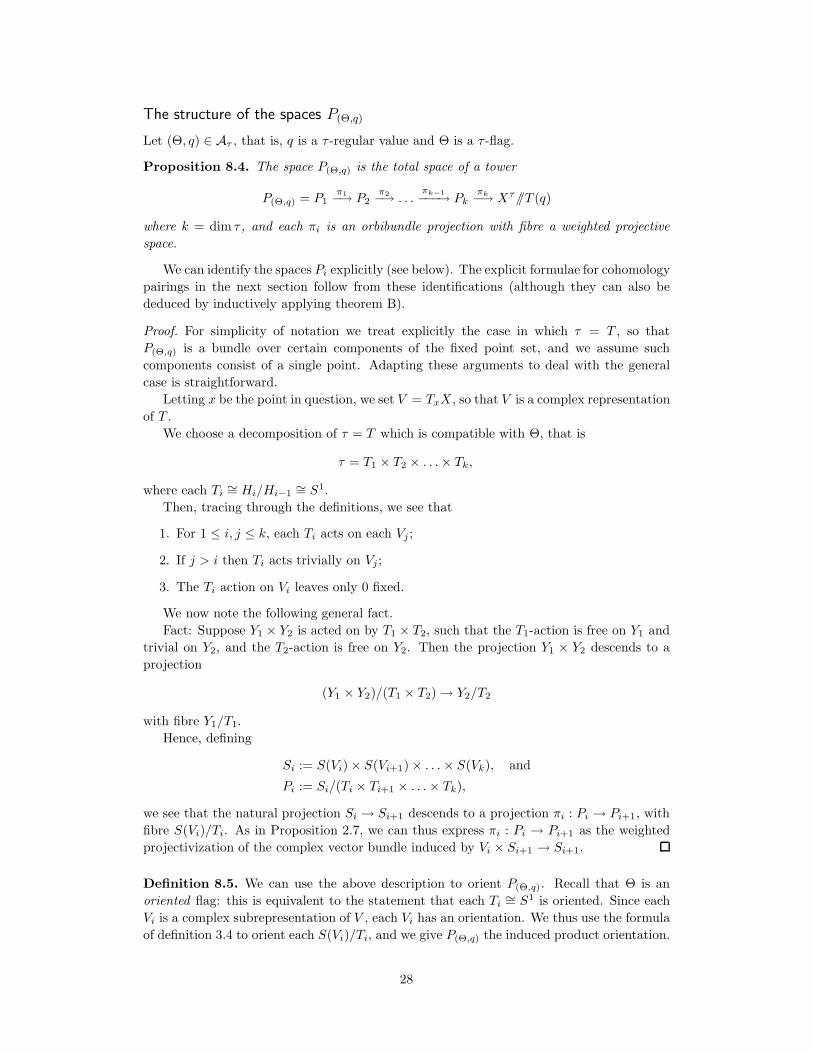
Proposition 8.4. The space P(Θ,q) is the total space of a tower

P(Θ,q) = P1π1−→ P2

π2−→ . . .πk−1−−−→ Pk

πk−→ Xτ//T (q)

where k = dim τ , and each πi is an orbibundle projection with fibre a weighted projective

space.

We can identify the spaces Pi explicitly (see below). The explicit formulae for cohomology

pairings in the next section follow from these identifications (although they can also be

deduced by inductively applying theorem B).

Proof. For simplicity of notation we treat explicitly the case in which τ = T , so that

P(Θ,q) is a bundle over certain components of the fixed point set, and we assume such

components consist of a single point. Adapting these arguments to deal with the general

case is straightforward.

Letting x be the point in question, we set V = TxX , so that V is a complex representation

of T .

We choose a decomposition of τ = T which is compatible with Θ, that is

τ = T1 × T2 × . . .× Tk,

where each Ti ∼= Hi/Hi−1∼= S1.

Then, tracing through the definitions, we see that

1. For 1 ≤ i, j ≤ k, each Ti acts on each Vj ;

2. If j > i then Ti acts trivially on Vj ;

3. The Ti action on Vi leaves only 0 fixed.

We now note the following general fact.

Fact: Suppose Y1 × Y2 is acted on by T1 × T2, such that the T1-action is free on Y1 and

trivial on Y2, and the T2-action is free on Y2. Then the projection Y1 × Y2 descends to a

projection

(Y1 × Y2)/(T1 × T2)→ Y2/T2

with fibre Y1/T1.

Hence, defining

Si := S(Vi)× S(Vi+1)× . . .× S(Vk), and

Pi := Si/(Ti × Ti+1 × . . .× Tk),

we see that the natural projection Si → Si+1 descends to a projection πi : Pi → Pi+1, with

fibre S(Vi)/Ti. As in Proposition 2.7, we can thus express πi : Pi → Pi+1 as the weighted

projectivization of the complex vector bundle induced by Vi × Si+1 → Si+1.

Definition 8.5. We can use the above description to orient P(Θ,q). Recall that Θ is an

oriented flag: this is equivalent to the statement that each Ti ∼= S1 is oriented. Since each

Vi is a complex subrepresentation of V , each Vi has an orientation. We thus use the formula

of definition 3.4 to orient each S(Vi)/Ti, and we give P(Θ,q) the induced product orientation.

28

9. Localizating integration formulae to the fixed points

In this section we show how the relations defined in section 7 correspond to integration

formulae. We begin by defining a map which generalizes the localization map λH defined in

section 5. We then state theorem D in terms of this map. We then give an explicit formula

for this localization map in terms of characteristic classes.

Definition 9.1. Let τ be a subtorus of T , and let Θ be an oriented τ -flag. Then we define

the map

λΘ : H∗T (X)→ H∗

T/τ (Xτ )

as follows. Firstly, in the case that τ = {1} is the trivial subtorus, so that Θ = (1 ⊂ T ) is

the trivial flag, then we define λΘ to be the identity map. Otherwise we set

λΘ := λHk/Hk−1◦ . . . λH2/H1

◦ λH1 .

Here Hi is the subtorus in the flag Θ:

Θ = (1 = H0 ⊂ H1 ⊂ H2 ⊂ . . . ⊂ Hk = τ ⊂ T ),

and

λHi/Hi−1: H∗

T/Hi−1(XHi−1)→ H∗

T/Hi(XHi)

is the localization map of definition 5.1, with data consisting of the triple

(XHi−1 , T/Hi−1, Hi/Hi−1). Recall that Hi/Hi−1∼= S1 is assumed to be oriented.

After stating theorem D we will give an explicit formula for λΘ using a decomposition

of T and characteristic classes.

Note that λΘ can equivalently be defined via integration over the fibre of the bundle

PΘ(νXτ )→ Xτ

in an analogous way to the definition of λH (definition 5.1).

Theorem D. Suppose∑

i

ci[Θi, qi] = 0 ∈ A/R, ci ∈ Z.

Then for any a ∈ H∗T (X),

∑

i

ci

∫

Xτi//T (qi)

κ(λΘi(a)) = 0.

where, for each i, the flag Θi is a τi-flag, and where κ is the relevant natural map from the

equivariant cohomology of a manifold to the ordinary cohomology of its symplectic quotient,

as described in the notation section of the Introduction.

Moreover, for each flag Θi, the class λΘi(a) only depends on the restriction of a to the

submanifold Xτi .

The proof consists of straightforward unwinding of the definitions, and can be seen to

either follow from theorem C, or from theorem B, using inductive arguments analogous to

those in the proof of theorem C. We give a concrete application of this theorem in section 12,

in which we calculate some cohomology pairings on the symplectic reduction of products of

CP2.

29

A formula for λΘ in terms of characteristic classes

Suppose Θ is an (oriented) T -flag of subtori (that is, we suppose τ = T ). We consider the

map

λΘ : H∗T (X)→ H∗(XT ).

We first observe that, for any component F ⊂ XT of the fixed point set and any class

a ∈ H∗T (X), the restriction of λΘ(a) to F only depends on the restriction of a to F (this

follows from the definition of λH).

Since T acts trivially on F , we have H∗T (F ) ∼= H∗(F ) ⊗H∗

T (pt). We choose a decompo-

sition

T = T1 × T2 × . . .× Td

compatible with the flag Θ, that is, where each Ti ∼= Hi/Hi−1∼= S1. This gives a set of

generators {u1, u2, . . . , ud} of H∗T (pt) so that

H∗T (F ) ∼= H∗(F )⊗Q[u1, u2, . . . , ud].

Explicitly, ui is the equivariant first Chern class of the representation of T on C where Tiacts with weight 1 (recall Ti is oriented), and the other Tj act trivially.

We now define the map

ℓi : Q[ui]→ H∗(F )⊗Q[ui+1, . . . , ud], by

uj+ki

i 7→ sTi+1×...×Td

j (Vi, Ti)

where ki + 1 = rkVi and sTi+1×...×Td

j (Vi, Ti) is the equivariant weighted Segre class (equiv-

ariant with respect to Ti+1 × . . .× Td) of the bundle Vi → F .

Then ℓi extends to a map

ℓi : H∗(F )⊗Q[ui, . . . , ud]→ H∗(F )⊗ Q[ui+1, . . . , ud]

by tensoring with the identity map on the complement of Q[ui]. Thus ℓi is a homomorphism

of H∗(F )⊗Q[ui+1, . . . , ud]-modules.

Now for any a ∈ H∗T (X), the restriction a|F can be decomposed

We then have

Proposition 9.2.

λΘ(a) = oT (X) · ℓd ◦ ℓd−1 ◦ . . . ◦ ℓ1(a|F ).

where oT (X) is the order of the maximal subgroup of T which fixes every point in X.

We will use this formula in the explicit calculations of section 12.

Proof. This follows by repeatedly applying proposition 6.3, using explicit identifications

coming from the choice of decomposition of T . For example, we have

Hi = T1 × T2 × . . .× Ti

and so on.

30

10. A more refined look at the module of relations

In section 7, we gave a number of definitions, culminating in the definitions of the modules

A and R. The aim of those definitions was to keep track of the relations arising from paths

as simply as possible. In this section we give ‘improved’ versions of these definitions. The

result of these improved definitions will be that A andA/R will be much smaller, and should

have properties which more accurately reflect the manifold X . The cost of this improvement

is that the definitions are somewhat more subtle.

This section contains no new results: its only aim is to give alternative definitions which

may be useful in some applications. Theorems C and D are still true with the improved

definitions given in this section.

Definition 10.1. We say an action of a Lie group G on a manifold Y is locally effective

if there is some point in Y whose stabilizer subgroup is finite.

Definition 10.2. Let τ ⊂ T be a subtorus. We denote by X [τ ] ⊂ Xτ the connected

components of Xτ on which the T/τ -action is locally effective.

Note that there are only finitely many subtori τ for which X [τ ] is nonempty.

Given this definition, we redefine the notions of a τ-regular point q, a τ-transverse

path Z, and the wall-crossing data of a τ -transverse path by substituting X [τ ] for Xτ in

definitions 7.2, 7.3 and 7.4.

Definition 10.3. Let V be a τ -representation, such that 0 ∈ V is the only fixed point. A

τ -flag Θ = (1 = H0 ⊂ H1 ⊂ H2 ⊂ . . . ⊂ Hk = τ) is called V -admissible if the associated

flag in V

V = V H0 ⊃ V H1 ⊃ . . . ⊃ V Hk = {0}

has each inclusion a strict inclusion.

Definition 10.4. Let τ be a subtorus of T , and let Θ be a τ -flag and q a τ -regular value

(using the version of τ -regular defined in this section). We say the pair (Θ, q) is admissible

if there is some point x ∈ X [τ ] ∩ µ−1(q) such that Θ is νxX[τ ]-admissible.

It is easy to see that the admissible pairs are precisely those pairs (Θ, q) for which the

space P(Θ,q) is nonempty.

Definition 10.5. We now redefine A to have generators the set of admissible pairs (Θ, q).

We will redefine the submodule of relations R to come from the data for τ -transverse paths,

as τ runs through all subtori, in the same way as before. However there is one difference:

some of the pairs which arise from the data of a path may not be admissible, and we simply

discard these pairs and construct relations from the pairs that remain. (The point is that

these pairs correspond to empty spaces, so there is no harm in discarding them). Explicitly,

if τ ⊂ T is a subtorus, Z is a τ -transverse path and Θ is an oriented τ -flag, then we take

the sum

−(Θ, q0) + (Θ, q1) +∑

(H,r)∈data(Z)

(Θ ∪H, r),

and throw out any terms in this sum which are not admissible pairs. We then define the

resulting sum to be a generator of R. (Here, as before, q0 and q1 are the endpoints of Z, and

Θ ∪H denotes the oriented H-flag defined by concatenating Θ and H , with H/τ oriented

as in data(Z).)

31

The statement that every element of A can be localized to the fixed points becomes

Proposition 10.6. A/R is generated by AT /(R∩AT ).

I conjecture

Conjecture 10.7. For any 0 ≤ i ≤ dimT , let Ai =⊕

dim τ=iAτ . Then A/R is generated

by Ai/(R∩Ai).

Question 10.8. Using the ‘improved’ definitions of this section, is the following ‘converse’

to theorem D true: Given a ∈ H∗T (XT ), suppose that, for every relation r ∈ R ∩ AT , the

sum of integrals of classes induced by a vanishes (as in theorem D). Then does a extend to

a class a ∈ H∗T (X)?

11. Calculations I: cohomology pairings on symplectic quotients of (S2)n

Consider the unit sphere S2 ⊂ R3. The Euclidean volume on R3 restricts to give a symplectic

form on S2 (with respect to which its volume is 4π). SO(3) acts naturally on S2, and this

action is Hamiltonian (it is possible to identify R3 with Lie(SO(3))∗ such that the inclusion

of S2 is a moment map). We choose a maximal torus S1 ⊂ SO(3) to be the subgroup which

fixes the north and south poles, and normalize so that the positive direction in S1 rotates

the sphere counterclockwise, as seen from the north pole.

Let X = (S2)n, the n-fold product, with the diagonal action of SO(3), and hence S1.

The symplectic form on X is given by the direct sum of the symplectic forms on the factors.

We will fix n to be odd, and calculate cohomology pairings on X//S1(0). We will also

invoke a formula proved in [23] to use these pairings to determine cohomology pairings on

(S2)n//SO(3).

The moment map

The action of S1 on S2 is Hamiltonian, with moment map given by the height function

µ : S2 → R

x 7→ ht(x).

We have µ(S2) = [−1, 1], µ(north pole) = 1, µ(south pole) = −1. Choosing a compatible

almost complex structure (for example the standard one), the weight of the action on the

tangent space at the north pole is 1, and the weight at the south pole is −1.

A point in (S2)n is given by an n-tuple (x1, . . . , xn) where each xi ∈ S2. The action of

S1 on (S2)n has moment map given by summing the heights on each of the factors:

µ(x1, . . . , xn) = ht(x1) + . . .+ ht(xn).

Thus µ((S2)n) = [−n, n].

A point in X is fixed if and only if each xi is either the north pole or the south pole.

Definition 11.1. Let I be any subset of the set {1, . . . , n}. Then we define the point

fI ∈ (S2)n by setting xi to be the south pole if i ∈ I and the north pole otherwise.

This defines a one-to-one correspondence between the fixed points and the subsets of

{1, . . . , n}. In particular, the fixed points are isolated, and we have

µ(fI) = n− 2|I|.

Hence 0 is a regular value of µ when n is odd.

32

The integration formula relating the symplectic quotients by a nonabelian group

and by its maximal torus

Suppose X is a symplectic manifold with a Hamiltonian action of the nonabelian Lie group

G, having moment map µG : X → Lie(G)∗. The inclusion T → G induces a projection

Lie(G)∗ ։ t∗, and composing of µG with this projection gives a moment map µT : X → t∗

for the action of T on X . In the companion paper [23] the following formula is proven,

relating integrals on X//G(0) =µ−1

G(0)

G to integrals on X//T (0) =µ−1

T(0)

T .

Proposition 11.2. For any a ∈ H∗G(X),

∫

X//G(0)

κ(a) =1

|W |

∫

X//T (0)

κ(a) ⌣∏

α∈∆

c1(Lα).

Here |W | denotes the order of the Weyl group, and ∆ ⊂ t∗ denotes the set of roots of G

(both positive and negative). Given a root α, then the complex line bundle Lα → X//T (0)

is the line bundle associated to the fibering µ−1T (0) → X//T (0) and the 1-dimensional T -

representation of weight α.

The volume of the symplectic quotient

Definition 11.3. The symplectic volume of a compact symplectic manifold (or orbifold)

(M2n, ω) is the integral∫M ωn/n!. From now on we will refer to the symplectic volume as

simply the volume.

We will now go through the calculations necessary to prove

Proposition 11.4. For n odd,

vol((S2)n//S1(0)) =(2π)n−1

(n− 1)!

n−12∑

k=0

(−1)k(n

k

)(n− 2k)n−1,

and

vol((S2)n//SO(3)) = −(2π)n−3

(n− 3)!

1

2

n−12∑

k=0

(−1)k(n

k

)(n− 2k)n−3.

X is endowed with a line bundle L → X (known in the literature as the prequantum

line bundle), with a connection whose curvature is −iω. Hence c1(L) =[ω2π

]. The action

on X lifts to an action on L. Hence the volume of X//S1(0) is given by

vol(X//S1(0)) =(2π)n−1

(n− 1)!

⟨κ(cS

1

1 (L)n−1), [X//S1(0)]⟩

where cS1

1 denotes the equivariant first Chern class (and, as usual, κ : H∗T (X)→ H∗(X//S1)

is the map described in the introduction.)

In order to evaluate classes on X//SO(3) we use the integration formula, proposition 11.2

of the companion paper [23]. We first need a definition. Let α be a weight of S1. Then we

denote by C(α) the representation induced by α, and set C(α) := X×C(α), thought of as an

equivariant line bundle over X . C(α) induces a line bundle on the quotient X//S1(0), which

we denote by L(α). Applying the integration formula, proposition 11.2, we have

vol(X//SO3)(0)) =

(2π)n−3

(n− 3)!

1

2

∫

X//S1(0)

κ(cS1

1 (L)n−3 ⌣ cS1

1 (C(1)) ⌣ cS1

1 (C(−1))).

33

The calculation

We now go through the steps necessary to evaluate cohomology classes on X//T (0). Steps

1-3 are independent of the particular class we wish to evaluate, and steps 4 and 5 depend

on the class.

Step 1: Fix Z, and enumerate the components Xq,i. We fix our submanifold Z to

be the interval [0, n+ 1], with p0 = 0 and p1 = n+ 1, which is outside the image of µ. Then

Z ∩ {walls} = {n− 2k | k = 0 . . .[n2

]}. For q = n− 2k,

{Xq,i} = {fI | |I| = k}.

(There are(nk

)such points.)

Step 2: Identify νXq,i. Our submanifolds are the points fI . The normal bundle to fI is

the direct sum of copies of TnS2 and TsS

2. Hence, with k = |I|,

νfI ∼= Cn−k(1) ⊕ Ck(−1)

Here Cm(w) denotes Cm with the S1-action with weight w. Note that the weights are deter-

mined by the isomorphism S1∼=−→ S1 induced by the orientation of Z; in our case this is

the identity isomorphism. (If we had instead chosen Z = [−n − 1, 0], we would have the

orientation-reversing isomorphism.)

Step 3: Calculate sw(νXq,i). The weighted Segre class lies in H∗T/H(Xq,i). In our case

this is just H∗(fI). We have

swj (νfI) =

{(∏{wts})−1 = (−1)k j = 0,

0 j > 0.

Since all the weights are ±1, we have hcf{|wts|} = 1.

Step 4: Calculate a in terms of local bases.

L|fI∼= C(µ(fI )) = C(n−2k).

Hence

cS1

1 (L)|fI= (n− 2k)u,

where u is the positive generator of H∗S1(pt). And

cS1

1 (C(w))|fI= wu, w ∈ Z.

The two classes we wish to evaluate are

a1 := cS1

1 (L)n−1

which gives us the degree of X//S1(0), and

a2 :=1

2cS

1

1 (L)n−3 ⌣ cS1

1 (C(1)) ⌣ cS1

1 (C(−1))

which gives the degree of X//SO(3). We thus have

a1|fI= (n− 2k)n−1un−1

and

a2|fI= −

1

2(n− 2k)n−3un−1.

34

Step 5: Apply the formula. Using the Segre classes calculated above, we have

λS1(a1)|fI= (−1)k(n− 2k)n−1

and

λS1(a2)|fI= −

1

2(−1)k(n− 2k)n−3

Hence, summing over the(nk

)points fI with |I| = k, and letting k run from 0 to

[n2

], we

get proposition 11.4.

Cohomology classes on (S2)n.

We wish to describe cohomology classes on X , and in particular understand their restrictions

to the fixed points. There are some standard results which will help us greatly. We first

recall these general results.

Let G be a compact Lie group, with T ⊂ G the maximal torus, and W the Weyl

group. For any G-space Y , there is a natural action of W on H∗T (Y ), and the natural map

H∗G(X)→ H∗

T (X) defines an isomorphism

H∗G(X)

∼=−→ H∗

T (X)W

(see e.g. [1, Equation 2.11]).

Suppose X1 and X2 are symplectic manifolds, with Hamiltonian actions of the group

G. Then the homotopy quotients (X1)G and (X2)G are cohomologially trivial as bundles

over BG [21, Proposition 5.8]. This means that the Serre spectral sequence of the fibering

(Xi)G → BG degenerates at the E2 term. We give the product X1 × X2 the diagonal

G-action. Then it follows that

H∗G(X1 ×X2) ∼= H∗

G(X1)⊗H∗(BG) H∗G(X2). (11.5)

In order to see this, we first note that X1 × X2 is both a Hamiltonian G-manifold (with

moment map given by the sums of the respective moment maps), and a Hamiltonian G×G

manifold. Now consider the diagonal map

j : BG → BG×BG.

This induces the ring homomorphism

H∗((X1)G)⊗H∗(BG) H∗((X2)G)→ H∗((X1)G ×BG (X2)G)

a, b 7→ j∗(a⊗ b).

But by degeneracy of the relevant spectral sequences, this must be an isomorphism of groups,

and hence an isomorphism of rings. Thus we have equation (11.5) above.

This means we can represent an equivariant cohomology class on X1 ×X2 as a sum of

tensor products of equivariant classes on X1 and X2. Now for our calculations we will only

need to know the restriction of a class to the fixed points. However restriction commutes

with the above tensor product (and the fixed point set of X1 × X2 is the product of the

fixed points of X1 with the fixed points of X2).

We now specialize to the case at hand. Let n denote the north pole and s the south pole

of S2. The restriction map

H∗S1(S2)→ H∗

S1({n, s})

35

is injective. We set

H∗S1({n, s}) = Q[un]⊕Q[us]

so that for example un is the degree-2 generator of the equivariant cohomology of {n}.

Then the image of the restriction consists of those pairs of polynomials whose degree-

zero terms agree. (One can see this e.g. by thinking about the topology of the homotopy

quotients.)

The SO(3)-equivariant cohomology is the subring invariant under the Weyl group, in

this case Z/2Z. The nontrivial element of W permutes the north and south poles and

simultaneously acts via the involution on S1. This identifies un with −us. Hence, fixing a

normalization,

H∗SO(3)(S

2) ∼= Q[v]

with the inclusion given by

Q[v] → Q[un]⊕Q[us]

a(v) 7→ a(un)⊕ a(−us).

Applying equation 11.5, we represent a class on X as a sum of tensor products of classes

on S2. Hence, consider the class

a(1) ⊗ a(2) ⊗ . . .⊗ a(n)

where a(i) is an equivariant cohomology class on the i-th copy of S2. We represent a(i)

as the pair of polynomials (a(i)n , a

(i)s ). A fixed point fI is an element of the set {n, s}n,

and the restriction of a(1) ⊗ a(2) ⊗ . . .⊗ a(n) to fI is simply the product of the appropriate

polynomials. (For example if I = ∅, then fI = (n, . . . , n), and the restriction to fI is∏ni=1 a

(i)n .)

We shall concentrate on evaluating classes on X//SO(3). Any such class is a linear

combination of classes of the form

a = vl11 ⊗ vl22 ⊗ . . .⊗ v

lnn .

a is of top degree when l1 + . . .+ ln = n−3. We now calculate a|fI. Define, for i ∈ {1 . . . n},

σ(i) =

{1, i /∈ I;

−1, i ∈ I.

Then

a|fI= (σ(1)u)l1 · . . . · (σ(n)u)ln

= u∑li

n∏

i=1

σ(i)li .

Applying the integration formula, and assuming∑li = n− 3,

∫

X//SO(3)

a = −1

2

n−12∑

k=0

(−1)k∑

|I|=k

(n∏

i=1

σ(i)li

).

36

It is clear that this expression only depends on the parity of the li, and is invariant under

permuting the S2 factors. This will allow us to deduce quite a lot, but for the moment we

will press on and derive an explicit formula. Define J ⊂ {1 . . . n} by

i ∈ J ⇐⇒ li odd

and set m = |J |. Then

∫

X//SO(3)

a = −1

2

n−12∑

k=0

(−1)k∑

|I|=k

(−1)|J∩I|

= −1

2

∑

|I|≤n−12

(−1)|I|(−1)|J∩I|.

Now since∑li = n − 3, at least one li = 0. By invariance we may as well assume J =

{1 . . .m}, and hence ln = 0. We can split the above sum into those I which contain n and

those which don’t. The resulting cancellations leave us with∫

X//SO(3)

a = −1

2

∑

K⊂{1...n−1}

|K|= n−12

(−1)|K|(−1)|K∩{1...m}|

= −1

2(−1)

n−12

∑

K⊂{1...n−1}

|K|=n−12

(−1)|K∩{1...m}|.

From this description one can easily derive explicit computational formulæ. Alternatively,

using the easily-described product structure in H∗SO(3)(X) and Poincare duality in the sym-

plectic quotient, we can see some classes whose image must vanish on the symplectic quo-

tient.

Proposition 11.6. Using the identification described above

H∗SO(3)((S

2)n) ∼= Q[v1, v2, . . . , vn]

and the natural ring homomorphism κ : H∗SO(3)((S

2)n)→ H∗((S2)n//SO(3)), we have

∫

(S2)n//SO(3)

κ(vl11 vl22 . . . vlnn )

= −1

2(−1)

n−12

∑

K⊂{1...n−1}

|K|=n−12

(−1)|K∩{1...m}|

=1

2(−1)

n−12

(n− 1n−1

2

)− 2

m2∑

j=0

(m

2j

)(n− 1−mn−1

2 − 2j

)

where∑

i li = n− 3 and m is equal to the number of odd li.

It follows, for example, that the ideal ker(κ) contains the elements v2i − v

2j .

12. Calculations II: volume of the symplectic quotient of (CP2)n

Generalities on CPk−1

Consider the defining representation of Uk on Ck.

37

The maximal torus T k ⊂ Uk consists of the diagonal matrices

{

eit1

eit2

. . .

eitk

| ti ∈ R}.

The moment map for the action of the maximal torus on Ck is

µ(z1, . . . zk) = −1

2(|z1|

2, . . . , |zk|2).

The centre

Z(Uk) = {

eit

. . .

eit

| t ∈ R}

acts, with moment map

µZ(z) = −1

2

∑|zi|

2.

We can take the symplectic quotient of Ck by Z(Uk) at any negative value, to get CPk−1

(with a scaled symplectic form). Henceforth, we let CPk−1 denote the symplectic manifold

Ck//Z(Uk)(−k). This is endowed with prequantum line bundle L → CPk−1 of degree k.

PUk acts on CPk−1, and the action lifts to L.

Let T denote the (k − 1)-torus. We identify T with the maximal torus of PUk via the

inclusion into Uk

T := {

eit1

. . .

eitk−1

} → {

eit1

. . .

eitk−1

1

}

The image of this inclusion is a slice: every element of T k decomposes in a unique way as

a product of elements of Z(Uk) and T , thus identifying T with the maximal torus of PUk.

Let t∗ ∼= Rk−1 have standard basis {e1, . . . , ek−1}. Then ej corresponds to the represen-

tation

ej :

eit1

. . .

eitk−1

7→ eitj

The T -action on CPk−1 has fixed points {Fj | j = 1 . . . k}, where Fj denotes the point

[0 : . . . : 1 : . . . : 0] (only the j-th coordinate nonzero). We henceforth let µ denote the

moment map for the action of T on CPk−1. The image of µ is the convex hull of the points

µ(Fj). And

µ(Fj) =

(∑k−1i=1 ei

)− kej , j < k

∑k−1i=1 ei j = k

38

The walls for µ have corresponding subgroups Hj∼= S1, for j = 1 . . . k. Hj stabilizes the

wall equal to the convex hull of the points {µ(Fi) | i 6= j}. We have

Hj = {

1. . .

eit

. . .

1

, t ∈ R} for j = 1 . . . k − 1

and

Hk = {

e−it

. . .

e−it

, t ∈ R}

We let Hj denote the above subgroup, with the isomorphismHj

∼=−→ S1 implied by the above

coordinates on Hj . We write Hj for the subgroup with the opposite isomorphism with S1.

A set of positive roots for PUk is given by {ei− ej | i < j ≤ k−1}∪{ei | i = 1 . . . k−1}.

The action of T on the normal bundle to the fixed point Fj is given by

νFj ∼=

{⊕i6=j C(ei−ej) ⊕ C(−ej), j ≤ k − 1

⊕i6=k C(ei), j = k

We now consider the diagonal action of PUk on (CPk−1)n, and hence of T ⊂ PUk. The

fixed points under the T -action are simply elements of the n-fold product of the fixed points

in CPk−1. Thus they correspond to partitions

{1 . . . n} = I1 ⊔ I2 ⊔ . . . ⊔ Ik

in the obvious way. We denote such a fixed point by

FI1,... ,Ik∈ (CP

k−1)n

Calculations on (CP2)n

We now specialize to CP2, setting X = (CP

2)n. We will calculate invariants of X//T (0) and

X//PU3, for n not a multiple of 3.

The fixed points correspond to partitions

{1 . . . n} = I1 ⊔ I2 ⊔ I3.

For n = 1 we have

µ(F1) = e2 − 2e1

µ(F2) = e1 − 2e2

µ(F3) = e1 + e2

Hence, in general

µ(FI1,I2,I3) = (−2|I1|+ |I2|+ |I3|)e1 + (|I1| − 2|I2|+ |I3|)e2.

It follows that 0 is a regular value as long as n is not a multiple of 3.

39

���� 6.........................................................................................................................................................................................

......................................................................................

............................................... ��6

jI1j > n3jI3j > n3jI2j < n3 p0=0

Zr1r2r3r4 r5

.............................................................6 � ��(F3)

�(F1) �(F2)� = e1

e2

Figure 5: The moment map for (CP2)4, showing the transverse paths used in the calculation, with their

wall-crossings.

We start by taking the path Z, as depicted in figure 12. In the case of (CP2)4, Z has 3

wall-crossings. The horizontal walls (in the figure) correspond to the subgroup

H2 = {

(1

eit

)| t ∈ R}

Z crosses these walls in in the same direction as e2, so that the isomorphism H2

∼=−→ S1 is the

standard one for H2, as described above. On the other hand, the vertical walls correspond

to the subgroup H1, and the direction of the crossing by Z corresponds to the oriented

subgroup H1.

Let Θ1 denote the flag

Θ1 = (H2, H2 × H1)

and let Θ2 denote the flag

Θ2 = (H1, H1 ×H2)

We then have, in the case n = 4,

p0 ∼ (r1,Θ1) + (r2,Θ1) + (r3,Θ1) + (r4,Θ1) + (r5,Θ2)

In general, let R1 denote the set of vertices corresponding to fixed points FI1,I2,I3 with

|I1| >n3 and |I3| >

n3 , and R2 the vertices corresponding to fixed points FI1,I2,I3 with

|I2| <n3 and |I3| <

n3 . We then have

p0 ∼∑

r∈R1

(r,Θ1) +∑

r∈R2

(r,Θ2). (12.1)

40

Fixing attention on the point FI1,I2,I3 , we now calculate the maps

λΘi: H∗

T (pt) = Q[u1, u2]→ H∗(pt) = Q

where u1 and u2 are the generators corresponding to H1 and H2. We have

V := νFI1,I2,I3∼= C

|I1|(e2−e1) ⊕ C

|I1|(−e1) ⊕ C

|I2|(e1−e2) ⊕ C

|I2|(−e2) ⊕ C

|I3|(e1) ⊕ C

|I3|(e2).

The subbundle stabilized by H2 is

V H2 = C|I1|(−e1) ⊕ C

|I3|(e1).

Hence, to calculate λΘ1 we need the equivariant weighted Segre classes of V/V H2 .

V/V H2 ∼= C|I1|(e2−e1) ⊕ C

|I2|(e1−e2) ⊕ C

|I2|(−e2)

⊕ C|I3|(e2).

Now the weighted Chern class

cH11 (C(ke1+le2)) = ku1

and hence

swH1(C(ke1+le2)) = (l + ku1)

−1

Therefore

swH1(V/V H2) = (1− u1)

−|I1|(u1 − 1)−|I2|(−1)−|I2|(1)−|I3|

= (1− u1)−(|I1|+|I2|)

and rk(V/V H2) = |I1|+ 2|I2|+ |I3|. Hence, setting k = rk(V/V H2), and l = |I1|+ |I2|,

λ(H2, H1, V/VH2) : uj2 7→

{0, j < k − 1(j+1−k+l−1

l−1

)uj+1−k

1 , j ≥ k − 1

By the functorial properties of integration over the fibre, this map commutes with mul-

tiplication by uj11 . To get λΘ1 we must compose with λ(H1, 1, VH2), which is equal to

−λ(H1, 1, VH2). We have

λ(H1, 1, VH2) : uj1 7→

{(−1)|I1|, j = |I1|+ |I3| − 1

0 otherwise

Hence

λΘ1(uj11 u

j22 ) =

{(−1)|I1|+1

(j2−|I2|−|I3||I1|+|I2|−1

), j2≥|I1|+2|I2|+|I3|−1

and j1+j2=2m−2

0 otherwise.

And similarly

λΘ2(uj11 u

j22 ) =

{(−1)|I2|+1

(j1−|I1|−|I3||I1|+|I2|−1

), j1≥2|I1|+|I2|+|I3|−1

and j1+j2=2m−2

0 otherwise.

41

The Volume

We can now easily write down formulæ for the evaluation of cohomology classes on (CP2)n//T .

And, by applying the integration formula from the companion paper [23] relating evaluation

of classes on G-symplectic-quotients to evaluation on T -symplectic-quotients, we can write

down formulæ for the evaluation of classes on (CP2)n//PU3. As an example, we will give a

formula for the volume of (CP2)n//PU3.

As usual, the ‘prequantum line bundle’ L → (CP2)n, which has first Chern class equal

to[ω2π

], descends to a line bundle over the symplectic quotient, which we also denote by L.

The dimension of (CP2)n//PU3 is 4n− 16, and hence the volume is equal to the evaluation

of the class (2πc1(L))2n−8

(2n−8)! against the fundamental class.

We define

a :=1

6(2n− 8)!(2πcS

1

1 (L))2n−8 ⌣∏

α∈∆

cS1

1 (C(α)),

where ∆ = {e1 − e2, e1, e2, e2 − e1,−e1,−e2} is the set of roots. Then we have

vol((CP2)n//PU3) =

∫

(CP2)n//T (0)

a

and, applying Theorem D and equation (12.1),

vol((CP2)n//PU3) =∑

(I1,I2,I3)|I1|>

n3 ,|I3|>

n3

λΘ1(a|FI1,I2,I3) +

∑

(I1,I2,I3)|I2|<

n3 ,|I3|<

n3

λΘ2(a|FI1,I2,I3)

where the triples (I1, I2, I3) run through partitions of {1 . . . n}. Given such a partition, set

i1 = |I1|, i2 = |I2|, i3 = |I3|. Then

L|FI1,I2,I3

∼= C(µ(FI1,I2,I3 ))

= C((−2i1+i2+i3)e1+(i1−2i2+i3)e2).

Hence

cS1

1 (L)∣∣∣FI1,I2,I3

= (−2i1 + i2 + i3)u1 + (i1 − 2i2 + i3)u2,

so that

a|FI1,I2,I3= ((−2i1 + i2 + i3)u1 + (i1 − 2i2 + i3)u2)

2n−8 · (2u31u

32 − u

41u

22 − u

21u

42).

Applying the formulæ for λΘ1 and λΘ2 , and using the identity 2(mk

)−(m+1k

)−(m−1k

)=

42

−(m−1k−2

), we easily derive the unilluminating but nontheless computable formula

(2n− 8)!

(2π)2n−8vol((CP2)n//PU3) =

∑

i1>n3 ,i3>

n3

i1+i3≤n

n!(−1)i1+1

i1!i3!(n− i1 − i3)!·

((2n− 8

i1 + i3 − 4

)(n− 3i1)

i1+i3−4(3i1 + 3i3 − n)2n−4−i1−i3(2 + i3 − n)−

(2n− 8

i1 + i3 − 3

)(n− 3i1)

i1+i3−3(3i1 + 3i3 − n)2n−5−i1−i3 −

i1+i3−5∑

j=0

(n+ i1 − 6− j

n− i3 − 3

)(2n− 8

j

)(n− 3i1)

j(3i1 + 3i3 − n)2n−8−j

+∑

i1<n3 ,i2<

n3

i1+i2≤n

n!(−1)i1+1

i1!i2!(n− i1 − i2)!·

((2n− 8

i1 + i2 − 4

)(n− 3i1)

i1+i2−4(3i1 + 3i2 − n)2n−4−i1−i2(2 + i2 − n)−

(2n− 8

i1 + i2 − 3

)(n− 3i1)

i1+i2−3(3i1 + 3i2 − n)2n−5−i1−i2 −

i1+i2−5∑

j=0

(n+ i1 − 6− j

n− i2 − 3

)(2n− 8

j

)(n− 3i1)

j(3i1 + 3i2 − n)2n−8−j

.

A. Orbifolds, orbifold-fibre-bundles, and integration over the fibre

The purpose of this appendix is to collect together a number of facts about orbifolds which we use in the paper.

These are all straightforward generalizations of standard results.

An orbifold is a generalization of a manifold, and can roughly be thought of as follows:

whereas an n-dimensional manifold is locally modelled on Rn, an n-dimensional orbifold

is locally modelled on the quotient of Rn by a finite group. Orbifolds were first defined

and studied by Satake in his announcement [26] and his paper [27] (Satake used the term

‘V -manifold’; the term ‘orbifold’ is due to Thurston). Our interest in orbifolds comes from

the fact that the wall-crossing-cobordism and its boundary are in general orbifolds (even

if we are interested in a symplectic quotient which is smooth, we may encounter orbifold

singularities after crossing a wall).

In this appendix we collect together facts involving orbifolds which we need in the rest

of the paper. These facts all involve integration on orbifolds, in one form or another,

and can be seen as straightforward generalizations of standard facts involving manifolds.

These generalizations exist because an orbifold is a ‘rational (co)homology manifold’, which

basically means that, if we take rational coefficients, it possesses the same homological and

cohomological properties as a manifold.

We begin by giving Satake’s definition of an orbifold, as well as his generalizations to

oriented and symplectic orbifolds. We then state the various facts involving orbifolds, and

indicate how these facts follow from results in the literature.

43

The definition of an orbifold

We now give Satake’s definitions. We do this to set up notation which we refer to in the rest

of the appendix, but also to make explicit some of the subtleties in the definition. These

subtleties are necessary for orbifolds to have the good properties that we need (such as a

rational fundamental class).

Definition A.1 (Satake [26, 27]). Let M be a Hausdorff topological space. A (C∞)

orbifold structure on M consists of a covering U of M by open sets, and for each open

set U ∈ U , an associated triple (U , GU , ϕU ), where

U is a connected open subset of Rn;

GU is a finite group of linear transformations mapping U to itself, such that the set of

points fixed by GU has codimension ≥ 2; and

ϕU is a continuous map U → U such that, for every x ∈ U and g ∈ GU , ϕU (gx) = ϕU (x).

We assume that the induced map GU\U → U is a homeomorphism.

Moreover, if U, V ∈ U are open sets such that U ⊂ V , then we are given an injective group

homomorphism βUV : GU → GV , and an inclusion iUV : U → V which is a diffeomorphism

onto its image, and which is equivariant with respect to the action of GU (and its image in

GV ), and such that ϕU = ϕV ◦ iUV . Finally, we assume that the open sets in U form a basis

for the topology of M . (It is fairly standard to refer to U as a local cover, GU as a local

group, and ϕU as a local covering map.)

An orbifold, then, is a space M together with an equivalence class of orbifold structures

on M (see Satake [26] for details of the straightforward notion of when two such sets of data

define the same orbifold structure).

By enhancing the definition of an orbifold structure, we can define an oriented orbifold:

we ask that each U be given an orientation which is preserved by the action of the group

GU , and that such orientations be compatible with the inclusions iUV : U → V .

Similarly, we define a symplectic orbifold by asking that each U be given a symplectic

form, with the same invariance and compatibility conditions.

Definition A.2. A point x of an orbifold M is a smooth point if there exists some open

set U ∈ U containing x, and such that the associated group GU is the trivial group. The

set of points which are not smooth points are called singular points.

Remark A.3. The set of smooth points of an orbifold M is connected (within each com-

ponent of M). More precisely, given any open set U ∈ U with associated triple (U , GU , ϕU ),

then the set of singular points in U is the image, under ϕU , of a finite union of submanifolds

of U having codimension ≥ 2. Each of these submanifolds is the submanifold of points fixed

by some nontrivial element g ∈ GU . (A straightforward argument by contradiction shows

that the codimension restriction on the fixed points of each local group GU implies the same

restriction for each nontrivial subgroup of GU , and hence for each nontrivial g ∈ GU ).

The fundamental class of an oriented orbifold

Fact A.4. Let M be an n-dimensional compact oriented orbifold (without boundary). Then

the orientation defines a rational fundamental class [M ] ∈ Hn(M) (recall that we are tak-

ing homology and cohomology with rational coefficients throughout this paper). Moreover,

M satisfies rational Poincare duality, which can be expressed as the fact that the pairing

44

Hi(M) × Hn−i(M) → Q given by (a, b) 7→∫Ma ⌣ b is a dual pairing on the rational coho-

mology of M .

The relationship between the orientation and the fundamental class is as follows. At any

smooth point x ∈M , we use the orientation to define a generator 1x ∈ Hn(M,M \ {x}) via

the identification with Hn(Rn,Rn \ {0}) ∼= Q given by excision (using an oriented chart).

Then the fundamental class is the unique class [M ] ∈ Hn(M) whose image under the natural

map Hn(M) → Hn(M,M \ {x}) has image 1x, for each smooth point x. (Since the set

of smooth points is connected, we actually only need to use one smooth point for each

component of M to get the right normalization.)

Sketch of proof. There are two different approaches to the proof. Satake’s approach [26, 27]

is to define an orbifold version of the de Rham complex3 and to prove de Rham’s theorem:

that the orbifold de Rham cohomology is canonically isomorphic to the singular cohomology

of M (with real coefficients). The fundamental class is then defined in terms of integration.

The other approach is to use the notion of a ‘rational homology manifold’, as described

by Borel in [4, chapters I–II]4. An orbifold is a rational homology manifold, and Borel shows

how various properties of the homology of manifolds go over to rational homology manifolds,

including the existence of a (rational) fundamental class and (rational) Poincare duality.

Oriented orbifolds with boundary and Stokes’s theorem

Satake defines an orbifold-with-boundary in [27, section 3.4]. His definition is equivalent to

modifying the definition of orbifold by allowing the open covers U to be open subsets of Rn

or of the halfspace Rn−1 × [0,∞) (but keeping the same conditions with respect to GU and

ϕU ). We then have

Fact A.5. Let M be an n-dimensional compact oriented orbifold-with-boundary. Then the

boundary ∂M is an (n−1)-dimensional orbifold, with a natural orientation induced from the

orientation of M , and ∂M is null-homologous in M (that is, the image of the fundamental

class [∂M ] is zero in Hn−1(M)).

Sketch of proof. In the language of differential forms, this is just Stokes’s theorem, and

the standard local argument applies (e.g. [3, theorem 3.5]). Alternatively, using the ratio-

nal (co)homology manifold approach, this fact follows from Poincare-Lefschetz duality [4,

chapter II].

Orbibundles and integration over the fibre

An ‘orbibundle’ is the natural orbifold version of a fibre bundle. Satake defined orbibundles

(he called them V -bundles).

Definition A.6 (Satake [27]). Let M be an orbifold, with orbifold structure defined by

the open cover U . An orbibundle over M is defined by giving, for each open set U ∈ U

3 A differential form on an orbifold M is a collection of differential forms on the sets U , invariant under

the local groups GU , and compatible with the inclusion maps in the obvious way; integration is defined

using a partition of unity and adding up integrals on sets U multiplied by the factors 1/|GU |.4A rational homology n-manifold is a space whose local homology, with rational coefficients, agrees

with that of an n-manifold (where the local homology at x ∈ M is H∗(M, M \ {x}). It’s an easy calculation

to show that an orbifold is a rational homology manifold. The construction of the rational fundamental

class of a rational homology manifold mimcs the usual construction: one shows that an orientation gives a

constant section of the local homology sheaf, and then applies a Mayer-Vietoris patching argument,(as in

[3, section 5] or [28, section 6.3]).

45

(with associated triple (U , GU , ϕU )) a GU -equivariant fibre bundle E → U . (Each inclusion

iUV must lift to a GU -equivariant bundle map, which is an isomorphism on the fibres.)

Given an orbibundle over M , there is an associated topological space (which we will refer to

as the total space) E with a map Eπ−→M defined so that π−1(U) = E/GU . An orbibundle

is oriented if the fibres of each bundle E → U are oriented (these orientations must be

preserved by the local groups GU and compatible with inclusion maps).

Remarks A.7. 1. Although the fibre of an orbibundle may be any space, in our appli-

cations the fibre will always be an orbifold.

2. The total space E of an orbibundle Eπ−→M is not in general a fibre bundle: if x is a

smooth point of M then π−1(x) will be a copy of the fibre F , but if x is an orbifold

point of M , then π−1(x) may be the quotient of F by a finite group.

We will describe the properties of a map on cohomology known as ‘integration over the

fibre’, but in order to do this, we must define the notion of a suborbifold.

Definition A.8. Given an orbifold M , then a suborbifold M ′ of M is defined by giving a

submanifold of each U , stable under GU and compatible with the inclusion maps, and such

that the restriction of the orbifold structure on M defines an orbifold structure on M ′ (in

particular, in each submanifold the set of points fixed by GU should have codimension ≥ 2).

It is important to note that, with this definition, a suborbifold M ′ of M consists mainly

of smooth points of M (more precisely, those points of M ′ which are smooth in M make up

a dense open subset of M ′). This is consistent with Satake’s definition of an orbifold, which

forces most points of an orbifold to be smooth points5.

Fact A.9. Let Eπ−→M be an orbibundle, with fibre the compact oriented orbifold F . Then

there is a map

π∗ : H∗(E)→ H∗−dimF (M)

known as integration over the fibre6 having the following properties:

1. Integration over the fibre is a module homomorphism of H∗(M)-modules (the module

structure is given by pullback via π followed by cup product). This is equivalent to the

‘push-pull formula’

π∗(π∗(a) ⌣ b) = a ⌣ π∗(b), ∀a ∈ H∗(E), b ∈ H∗(M).

2. Let i : M ′ → M be the inclusion of a suborbifold of M , and let E′ π′

−→ M ′ denote

the orbibundle over M ′ defined by the restriction of E. Then the following square

commutes:

H∗(E′)

π′

∗

��

H∗(E)

π∗

��

i∗oo

H∗−dimF (M ′) H∗−dimF (M).i∗oo

5It would be possible to give an alternative definition of an orbifold which removed these restrictions.

Specifically, given a local triple (U , GU , ϕU ), we could remove the restriction that the set of points fixed by

the GU -action on U have codimension ≥ 2, and alter the rest of the definition in a compatible manner. This

alternative definition would be more natural in some respects, but it would also be more involved, since we

would then need to take into account various numerical factors.6often referred to as the Gysin map (it generalizes the Gysin map defined for a sphere bundle) or, in a

more general setting, the pushforward.

46

(where i : E′ → E is the lift of i).

3. If E,M and F are compact oriented orbifolds, and the orientation of E equals the

product of the orientations of M and F , then for any class a ∈ H∗(E) we have

∫

E

a =

∫

M

π∗(a).

Sketch of proof. We again indicate two different proofs. Using differential forms, the usual

formula for integration over the fibre is well-defined on the local bundles E → U (this was

defined by Lichnerowicz [22], and is also explained by Bott and Tu [3, p. 61]; of course we

are using fact A.4, allowing us to integrate over the orbifold fibres). It is easy to check that

this gives GU -invariant differential forms on the sets U , and hence orbifold differential forms

on M (see fotnote 3). The advantage of this approach is that the three properties we have

listed above follow immediately from the definition.

Alternatively, in the manifold case, integration over the fibre can be defined using the

Leray-Serre spectral sequence of the fibration (described for sphere bundles quite explicitly

in Bott and Tu [3, pp. 177–179]). For an orbibundle Eπ−→ M we use the Leray spectral

sequence (with rational coefficients) of the map π [3, pp. 179–182], trivializing the the

top cohomology sheaf of the fibres by the rational fundamental classes on the local covers

E → U . Finally, the algebraic and naturality properties of the Leray-Serre spectral sequence

which imply properties 1-3 above also carry over to the Leray spectral sequence (see e.g.

McCleary [24]).

Remark A.10. We also need a related result concerning integration over the fibre: this

time for an (honest) fibre bundle Eπ−→ B, with fibre an oriented orbifold F , but where

the base space B may be any CW-complex. Using the same arguments as above, it is easy

to show that integration over the fibre π∗ is well-defined for such bundles, and satisifes

properties 1 and 2.

How orbifold-fibre-bundles can arise as locally free quotients of manifolds

Fact A.11. Suppose the compact connected Lie group G acts on a compact oriented man-

ifold N with a locally free action (that is, the stabilizer subgroup of each point is finite).

Then the quotient space N/G can be given an oriented orbifold structure (the orientation is

fixed by orienting G).

This orbifold structure on N/G is constructed by taking local slices for the action

(for the existence and properties of local slices, see for example Bredon [5, Chapter IV],

Kawakubo [19, section 4.4], or the chapter by Palais [4, chapter VIII]). Specifically, given a

point x ∈ N , then there exists a linear slice for the G-action at x: a submanifold S ⊂ N

which is transverse to the G-orbits, is mapped to itself by the stabilizer subgroup Gx, and

is equivariantly identified with an open subset of Rn with respect to a linear action of Gxon Rn. Letting F denote the subgroup of Gx which fixes every point in S, then the triple

(S,Gx/F, ϕ) defines the orbifold structure at [x] ∈ N/G (where ϕ maps S to S ·G ⊂ N/G).

The following existence facts follow easily from the definition of orbifold together with

simple arguments involving local slices.

Facts A.12. 1. If N ′ is an oriented submanifold of N , stable under G and transverse to

the submanifolds NH , for each finite subgroup H ⊂ G, then N ′/G is a suborbifold of

N .

47

2. If N is an oriented manifold-with-boundary on which the compact connected Lie group

G acts, with a locally free action, then N/G is an oriented orbifold-with-boundary.

3. Suppose E and N are oriented manifolds, and E → N is a fibre bundle. Then if G

and H are compact connected Lie groups, and G×H acts on E, covering an action of

H on N , and these actions are locally free, then E/(G×H)→ N/H is an orbibundle.

B. Cohomology and integration formulae for weighted projective bundles

The purpose of this appendix is to give generalizations of two classical formulae concerning

projective bundles. Let Y be a CW-complex, let V → Y be a complex vector bundle, and

let P(V ) → Y be its projectivization [3, p. 269]. The first classical formula describes the

cohomology of P(V ), and the second (and perhaps less well-known) calculates integrals over

the fibres of the bundle P(V )→ Y .

The generalizations we give apply to bundles constructed as follows. Let V → Y be

a complex vector bundle, and suppose S1 acts on V , such that the action is linear on the

fibres of V (that is, the action covers the trivial action on Y ), and such that the set of fixed

points equals the zero section. We consider the bundle S(V )/S1 π−→ Y , where S(V ) denotes

the unit sphere bundle in V , relative to some invariant metric.

These bundles can be considered as generalizations of projective bundles in the following

sense. If S1 acts with ‘weight one’ on the fibres (i.e. the standard multiplication action of

S1 ⊂ C×), then each S1-orbit lies in precisely one line in V , and identifying S1-orbits with

lines induces a isomorphism S(V )/S1 ∼= P(V ). The general case that we consider allows

any combination of positive and negative weights. This general case includes ‘weighted

projectivizations’ which correspond to S1 actions having only positive weights (Kawasaki

calculates the cohomology of weighted projective spaces in [20]; for some definitions and

results in algebraic geometry on weighted projective spaces, see [7]).

We begin by reviewing the cohomology and integration formulae in the case of projective

bundles. We then state and prove the general cohomology formula, followed by the general

integration formula. Finally, using the homotopy quotient construction, we will observe that

all the definitions, formulae, and proofs naturally extend to the case in which an auxilliary

group G acts on V and Y , commuting with the S1-action and with the projection.

Projective bundles

The projectivization P(V ) possesses a distinguished cohomology class h ∈ H2(P(V )), which

is usually defined as follows. Let S → P(V ) denote the tautological line bundle (where

the fibre of S over a point is just the corresponding line in V ), and define h to be the first

Chern class of the dual line bundle, h = c1(S∗).

Then the cohomology of P(V ) is given by the formula7

H∗(P(V )) ∼=H∗(Y )[h]

〈c0(V )hr + c1(V )hr−1 + . . .+ cr(V )〉.

where ci(V ) ∈ H2i(Y ) is the i-th Chern class, and r = rk(V ). In this formula the product

ahi (where a ∈ H∗(Y )) is identified with the class (π∗a)hi ∈ H∗(P(V )).

The vector bundle V → Y has associated Segre classes si(V ) ∈ H2i(Y ). The total Chern

class and the total Segre class are multiplicative inverses to each other (in the cohomology

7Bott and Tu [3, pp. 269-271] describe the projectivization and the tautological line bundle, and following

Grothedieck, they define the Chern classes in terms of the cohomology formula.

48

ring of Y ), that is

c(V )s(V ) = 1,

and this can be used to define the Segre classes in terms of the Chern classes. (As an

example, consider the tautological line bundle S → CPn. Then c(S) = 1− h, where h is the

generator of H∗(CPn), and s(S) = (1− h)−1 = 1 + h+ h2 + . . .+ hn.)

The integration formula expresses integrals over the fibres in terms of Segre classes:

π∗(hi) =

{0 i < rk(V )− 1,

si−rk(V )+1(V ), i ≥ rk(V )− 1,

where π∗ denotes integration over the fibre (see fact A.9). (This formula is sufficient to

calculate the integral over the fibres of any class on P(V ), since every class can be expressed

in the form (π∗a)hi, and we have π∗((π∗a)hi) = aπ∗(h

i).)8

Weighted Chern classes and the cohomology formula

We now return to the general case: V → Y is a complex vector bundle, with an action of

S1 on V , covering the trivial action on Y , and such that the set of fixed points equals the

zero section.

We first define the weighted Chern class of the pair (V, S1) (although we will sometimes

abuse notation and simply refer to this as the weighted Chern class of V ). We will then

state and prove a formula for the cohomology of the total space of the bundle S(V )/S1 π−→ Y

(where S(V ) denotes the unit sphere bundle in V relative to some invariant metric).

Definition B.1. The quick definition of the weighted Chern class is this: the weighted

Chern class cw is multiplicative under direct sum of bundles, and commutes with pullbacks

(so that the splitting principle applies), and for a line bundle L acted on with weight i, is

given by cw(L) = i+ c1(L) (where c1(L) is the regular first Chern class).

Explicitly, under the S1 action, V splits into ‘isotypic’ subbundles

V ∼=⊕

i∈Z

Vi,

where S1 acts with weight i on Vi (that is, λ ∈ S1 acts on Vi by multiplying the fibre

coordinates by λi). Then the weighted Chern class of (V, S1), which we denote cw(V ) ∈

H∗(Y ), is the product

cw(V ) :=∏

i

cw(Vi),

where, setting r equal to the rank of Vi,

cw(Vi) = ir + ir−1c1(Vi) + ir−2c2(Vi) + . . .+ cr(Vi)

(here cj(Vi) is the regular j-th Chern class of Vi). It follows from the properties of the

regular Chern class that the weighed Chern class is natural with respect to pullbacks, and8The integration formula might appear to be overkill: since it follows from the cohomology formula that

every class on P(V ) can be expressed as (π∗a)hi for 0 ≤ i ≤ rk(V )− 1, in fact we only need to observe that

π∗(hi) = 0 for 0 ≤ i ≤ rk(V )− 1, and π∗(hrk(V )−1) = 1. However in applications we are often given a class

on P(V ) expressed as (π∗a)hi where i is not necessarily in this range. Using the cohomology formula, we

could rewrite such a class in terms of the cohomology of Y and the classes {1, h, h.., hrk(V )−1}, in which

case the integral over the fibres would be the coefficient of hrk(V )−1. The integration formula is simply the

answer one gets by following this process.

49

multiplicative with respect to direct sum (it is easiest to think of the S1-action as simply

decomposing V into a direct sum of subbundles, each of which is labelled with an integer,

and to note that this decomposition commutes with pullback and direct sum in an obvious

way).

Proposition B.2. Let V → Y be a complex vector bundle with an action of S1 as above.

Define h ∈ H2(S(V )/S1) to be the first Chern class of the principal orbifold bundle S(V )→

S(V )/S1 (see remark B.3 below). Then there is a ring isomorphism

H∗(S(V )/S1) ∼=H∗(Y )[h]

〈cw0 (V )hr + cw1 (V )hr−1 + . . .+ cwr (V )〉,

induced by identifying a product ahi, where a ∈ H∗(Y ), with the class (π∗a)hi ∈ H∗(S(V )/S1).

Remark B.3. Suppose S1 acts with weight one on the fibres, so that we have a natural

isomorphism S(V )/S1 ∼= P(V ). Then the two definitions of the class h agree: the classical

definition, as the first Chern class of the dual of the tautological line bundle over P(V ), and

the definition in the above proposition. (The above definition of h is equivalent to defining

h as the first Chern class of the associated orbifold line bundle S(V )×S1 C(1) → S(V )/S1,

where C(1) denotes C with the weight one action of S1. In the classical case, it is easy

to show that this associated line bundle is isomorphic to the dual of the tautological line

bundle.)

Proof of Proposition B.2. This proof comprises two steps. We first identify the weighted

Chern classes of (V, S1) as certain coefficients of an equivariant Euler class. We then show

how this equivariant Euler class appears in a standard long exact sequence, and how the

properties of this long exact sequence give us the proposition.

Step 1: Relating cw(V ) to an equivariant Euler class. The S1-equivariant bundle

V → Y has an S1-equivariant Euler class

eS1(V ) ∈ H∗S1(Y ) ∼= H∗(Y )⊗H∗(BS1),

which we claim is given by

eS1(V ) = cw0 (V )ur + cw1 (V )ur−1 + . . .+ cwr (V ), (B.4)

where u ∈ H2(BS1) denotes the positive integral generator. (We briefly recall the definition

of the equivariant Euler class. The equivariant cohomology of Y is defined to be the regular

cohomology of the homotopy quotient YS1 = (Y × ES1)/S1. An equivariant vector bundle

V → Y pulls back to an equivariant vector bundle over Y × ES1, and by the quotient

construction induces a regular vector bundle over YS1 ; the equivariant Euler class of V is

defined to be the regular Euler class of this induced bundle.)

To show the above relationship between eS1(V ) and cw(V ), we first show that it holds

for line bundles. We then appeal to the splitting principle to extend this to vector bundles.

Suppose L → Y is a complex line bundle, possessing an action of S1 covering a trivial

action on Y . Let i ∈ Z equal the weight of the action of S1 on the fibres of L. Let L(0) → Y

denote the same line bundle, but with a trivial action of S1, and let C(i) → Y denote the

trivial line bundle with a weight-i action of S1. Then

L ∼= L(0) ⊗ C(i)

50

(as S1-equivariant line bundles). Hence, since Euler classes add when we tensor line bundles,

eS1(L) = eS1(L(0)) + eS1(C(i))

= c1(L) + iu

= cw1 (L) + cw0 (L)u.

This proves our claim (equation (B.4)) for line bundles, and the general case follows from

the splitting principle, together with the observation that both sides of equation (B.4) are

multiplicative with respect to direct sum of the vector bundles we are considering.

Step 2: The map H∗S1(Y )→ H∗(S(V )/S1). Let p and π denote the maps

S(V )/S1

//

p!!D

DDDD

DDD

S(V )/S1

π{{vvvvvvvvv

Y

and let /S1 denote the natural identification in equivariant cohomology H∗S1(S(V ))

/S1

−−→∼=

H∗(S(V )/S1).

Then, by naturality of this isomorphism, together with the definition of h, we have

(p∗(aui))/S1 = (π∗a)hi

for any a ∈ H∗(Y ).

But the natural map (p∗·)/S1 fits into a short exact sequence of H∗(Y )-modules

0 // 〈eS1(V )〉�

� // H∗S1(Y )

(p∗·)/S1

// // H∗(S(V )/S1) // 0, (B.5)

where 〈eS1(V )〉 ⊂ H∗S1(Y ) denotes the ideal generated by eS1(V ).

These properties follow from the existence of the long exact sequence in equivariant

cohomology for the pair (V, S(V )), together with the following identifications:

. . . // H∗S1(V, S(V )) // H∗

S1(V )

∼=

��

// H∗S1(S(V ))

∼= /S1

��

// . . .

H∗S1(Y )

∼= ⌣Φ

OO

⌣eS1 (V )

// H∗S1(Y )

p∗88ppppppppppp

// H∗(S(V )/S1)

Here the leftmost identification (denoted ⌣ Φ) is the Thom isomorphism in equivariant

cohomology, with Φ the Thom class (see [1, section 2] for more on this identification); the

next identification is induced by restriction to the zero-section of V , and is an isomorphism

because of the homotopy equivalence between V and Y . The restriction of the Thom class

Φ to the zero section equals the equivariant Euler class eS1(V ), and hence the composition

of the Thom isomorphism with the restriction is given by multiplication by the equivariant

Euler class on H∗S1(Y ). The remaining maps are easily identified as labelled. Finally, using

our explicit identification of the Euler class eS1(V ), we see that multiplication by this Euler

class is injective, and thus the sequence is short exact.

Hence we have

H∗(S(V )/S1) ∼=H∗S1(Y )

〈eS1(V )〉,

and, substituting our formula for eS1(V ), we have proven the proposition.

51

Weighted Segre classes and the integration formula

We now prove a formula which calculates integrals over the fibres of the bundle S(V )/S1 π−→

Y . This formula involves the ‘weighted Segre classes’ of the pair (V, S1), which we define.

We must also define an orientation of the fibres of π, so that integration over the fibre is

well-defined. In the case that S(V )/S1 can be naturally identified with a weighted projective

bundle (i.e. if the weights of the S1-action are all positive) this orientation agrees with the

standard orientation induced by the complex structure on the fibres.

Definition B.6. Let V → Y be a complex vector bundle with an action of S1 as above.

The condition that the set of points fixed by the action equals the zero section is equivalent

to the condition that no subbundle of V be acted on with weight zero. It follows that the

total weighted Chern class of (V, S1) is invertible in the rational cohomology ring of Y (since

the degree-zero component is nonzero), and we define the weighted Segre class to be its

multiplicative inverse:

sw(V )cw(V ) = 1.

Definition B.7. Given any point y ∈ Y , let Vy denote the fibre of V over the point y.

Then, for any v ∈ S(Vy), we have the isomorphism

TS1·v(S(Vy)/S1)⊕ R+ · v ⊕ s1 ∼= Vy,

where R+ · v ⊂ Vy denotes the ray from the origin through v, and s1 is the Lie algebra

of S1, identified with R in the standard way. We define the orientation of S(Vy)/S1 to be

that orientation which is compatible with the above isomorphism together with the given

orientations of R+, s1, and Vy (where Vy has the standard orientation defined by its complex

structure, as in equation (0.3)).

Proposition B.8. Let Y be connected and V → Y be a complex vector bundle with an

action of S1 as above. Consider the bundle S(V )/S1 π−→ Y , and define h ∈ H2(S(V )/S1) to

be the first Chern class of the principal orbifold bundle S(V )→ S(V )/S1 as in proposition

B.2 above. Then, for any a ∈ H∗(Y ),

π∗((π∗a) ⌣ hi

)=

{0 i < rk(V )− 1,

ka ⌣ swi−rk(V )+1(V ), i ≥ rk(V )− 1.

Here π∗ denotes integration over the fibre with respect to the orientation defined above, and

k is the greatest common divisor of the absolute values of the weights appearing in the S1

action on the fibres of V .

Proof. This proof consists of two steps. In step 1 we relate the rational fundamental class

of the fibres with the fundamental class of complex projective space. Then, in step 2, we

use the formula from proposition B.2 above.

Step 1: The rational fundamental class of the fibres of S(V )/S1 → Y . Given

y ∈ Y , let Vy denote the fibre of V over the point y. Then S1 acts on Vy, and we can make

an S1-equivariant identification

Vy ∼= Cr(i1,i2,... ,ir),

52

where Cr(i1,i2,... ,ir) denotes Cr with the weight-(i1, i2, . . . , ir) action of S1 (that is, λ ∈

S1 ⊂ C× acts by λ · (z1, . . . , zr) = (λi1z1, . . . , λirzr).) Moreover, we can arrange that

i1, . . . , in < 0 and in+1, . . . , ir > 0. Then the map

ϕ : Cr(1,1,... ,1) → Vy = Cr(i1,i2,... ,ir)

(z1, . . . , zr) 7→ (z|i1|1 , . . . , z

|in|n , zn+1

in+1 , zrir )

is smooth and intertwines the S1-actions.

There is an obvious S1-invariant metric on Vy = Cr(i1,i2,... ,ir) such that ϕ maps the

standard unit sphere in Cr(1,1,... ,1) to the unit sphere in Vy.

Hence ϕ descends to a map

ϕ : S(Cr(1,1,... ,1))/S1 = CP

r−1 → S(Vy)/S1.

We can now relate the rational fundamental class of S(Vy)/S1 to the fundamental class of

CPr−1 by calculating the oriented degree of ϕ (that is, the topological degree of ϕ, multiplied

by ±1 according to whether ϕ preserves or reverses orientation).

We easily see that the oriented degree of ϕ equals∏rj=1 ij = cw0 (V ) (and this also equals

the oriented degree of the restriction of ϕ to the unit sphere). To calculate the degree of

ϕ, we must divide this number by the degree with which a generic S1-orbit in S(Cr(1,1,... ,1))

covers its image. It is easy to see that this degree equals the greatest common divisor of the

absolute values of the ij. Hence, setting

k := gcd(|i1|, |i2|, . . . , |ir|)

then the oriented degree of ϕ is given by

deg(ϕ) = k−1cw0 (V ). (B.9)

Now consider the maps

CPr−1ϕ // S(Vy)/S

1 �

� ψ //

π′

��

S(V )/S1

π

��y �

� // Y

We have defined the class h ∈ H∗(S(V )/S1) to be the first Chern class of the orbifold

S1-bundle S(V ) → S(V )/S1. (Or equivalently, h is the first Chern class of the associated

orbifold line bundle S(V )×S1 C(1) → S(V )/S1, where C(1) denotes C with the weight-one

action of S1.) By naturality of this definition, we see that h pulls back to the integral

generator of the cohomology of CPr−1, so that∫

CPr−1

(ϕ∗ψ∗h)r−1 = 1.

Using the degree of ϕ, we thus have

π′∗((ψ

∗h)r−1) = kcw0 (V )−1,

and hence, since integration over the fibre commutes with restriction, and the result is a

degree-zero cohomology class, we have

π∗(hr−1) = kcw0 (V )−1 ∈ H0

G(Y ). (B.10)

(Of course π∗(hi) = 0 if i < r − 1, for degree reasons.)

53

Step 2: Using the relation in cohomology to extend this formula to all powers

of h. We now calculate

π∗((π∗cw(V )) ⌣ (1 + h+ h2 + h3 + . . . )

). (B.11)

Since π∗ lowers degree by 2r−2, we only need to consider terms in the product (π∗cw(V )) ⌣

(1 + h+ h2 + h3 + . . . ) of degree 2r − 2 and greater. The degree 2r − 2 term is

π∗cwr−1(V ) + π∗cwr−2(V )h+ . . .+ π∗cw0 (V )hr−1,

and applying π∗ to this term gives the coefficient of hr−1, multiplied by π∗(hr−1) (which we

have calculated in equation (B.10) above). (We are using the fact that π∗ is a homomorphism

of H∗(Y )-modules.) Hence, the integral over the fibre of the degree 2r−2 term of the product

(B.11) equals k ∈ H0(Y ).

The degree 2r term of the product (B.11) is

π∗cwr (V ) + π∗cwr−1(V )h+ . . .+ π∗cw0 (V )hr.

Comparing with our explicit identification of eS1(V ) in equation (B.4) above, we see that

this term is exactly the class p∗ (eS1(V )) /S1, and, using the short exact sequence (B.5),

this term vanishes. Similarly, the degree 2(r + j) term equals p∗(ujeS1(V )

)/S1 and hence

also vanishes. Thus we have

π∗((π∗cw(V )) ⌣ (1 + h+ h2 + h3 + . . . )

)= k

and hence (using the module-homomorphism property of π∗)

π∗(1 + h+ h2 + h3 + . . . ) = kcw(V )−1 = ksw(V ).

The proposition now follows by identifying terms by degree.

Equivariant weighted Segre classes, and the equivariant integration formula

Suppose V → Y is a vector bundle, with an action of S1 as above, and suppose moreover

that an auxilliary group G acts on V and Y , commuting with the projection and with the

action of S1. Then we can generalize the definition of weighted Chern classes and weighted

Segre classes to the G-equivariant case as follows.

Recall that the homotopy quotient construction replaces a G-space Y with the space

YG := EG×G Y , and the equivariant cohomology of Y is defined to be the ordinary coho-

mology of YG. Given a G-equivariant vector bundle V → Y the same construction gives

a vector bundle VG → YG (this is explained by Atiyah and Bott in [1, section 2: equation

(2.1) and remark (1)]), and the G-equivariant characteristic classes of V are then taken to be

the ordinary characteristic classes of VG → YG, which thus take values in the G-equivariant

cohomology of Y .

Definition B.12. In our case, in the presence of a commuting S1-action, the bundle VG →

YG has an induced S1-action, and we define the G-equivariant weighted Chern classes

and the G-equivariant weighted Segre classes of the pair (V, S1) to be the weighted

Chern classes and weighted Segre classes of the pair (VG → YG, S1) (definitions B.1 and

B.6).

54

Applying the cohomology formula (Proposition B.2) to the bundle VG → YG and making

the obvious identifications, we thus get the equivariant version of the cohomology formula:

H∗G(S(V )/S1) ∼=

H∗G(Y )[h]

〈cw0 (V )hr + cw1 (V )hr−1 + . . .+ cwr (V )〉, (B.13)

where cWi (V ) now denotes the i-th G-equivariant weighted Chern class of (V, S1). Similarly,

the integration formula (Proposition B.8) applied to VG → YG gives the (formally identical)

equivariant formula:

π∗((π∗a) ⌣ hi

)=

{0 i < rk(V )− 1,

ka ⌣ swi−rk(V )+1(V ), i ≥ rk(V )− 1,(B.14)

where sWi (V ) now denotes the i-th G-equivariant weighted Segre class of (V, S1).

C. Proof of the orientation lemma

We now give the proof of lemma 3.6, which describes the orientations of the boundary

components of the wall-crossing-cobordism.

Lemma C.1 (Lemma 3.6). Let the wall-crossing-cobordism W/T be oriented as in defi-

nition 3.2. Then the induced boundary orientation of X//T (p0) is −(ωkp0), and of X//T (p1)

is ωkp1 (where ωpidenote the respective induced symplectic forms), and the induced boundary

orientation of each P(H,q) is equal to the product orientation defined in 3.5 above.

Proof. Before beginning the proof proper, we fix three conventions which will hold through-

out the proof.

1. Most of the steps in this proof consist of exhibiting isomorphisms of the form

V1 ⊕ V2∼= V3,

where the Vi are vector spaces. For each such isomorphism, we will be using orientations

of two of the vector spaces to induce an orientation on the third, in the obvious manner

(explicitly: so that concatenating oriented bases for V1 and V2 gives an oriented basis for

V3).

2. When we decompose tangent spaces, we will assume without explicit mention that

these decompositions are orthogonal decompositions relative to some choice of invariant

metric; and it will always be the case that the induced orientations are independent of the

choices made.

3. Finally, given a symplectic form (that is, a nondegenerate 2-form) on any vector space,

then the symplectic orientation of that vector space will mean the orientation defined

by the top power of the symplectic form.

We break the proof up into two steps. In step 1 we assume that T is 1-dimensional, and

in step 2 we reduce the general case to to the case treated in step 1.

Step 1: Assuming T is 1-dimensional. If T is 1-dimensional, then Z is just a closed

subinterval of t, bounded by p0 and p1. The orientation of Z (definition 2.1) and of each

wall-crossing subgroup (which is just T itself) orients t so that p0 < p1. We orient t∗

compatibly (that is, so that the duality pairing between a positive vector in t and a positive

vector in t∗ is positive).

55

Then, restating definition 3.2 in this case, we have oriented the wall-crossing-cobordism

W/T via the isomorphism

T[x](W/T ) ∼= T[x]X//T (p)⊕ t∗ (C.2)

for each x ∈ W (with p = µ(x)), relative to the orientation of t∗ described above and the

symplectic orientation of X//T (p).

The key calculation in step 1 is to compare this orientation of W/T with the symplectic

orientation of X . Now at each x ∈ W , we can decompose TxW = TxX into the orbit

direction and its orthgonal complement. Using the natural identifications, then we claim

that

TxX = TxW ∼= T[x](W/T )⊕ t, (C.3)

is orientation-preserving, where t denotes t with the opposite orientation. Using equation

(C.2) above, this is equivalent to showing that the isomorphism

TxX ∼= T[x]X//T (p)⊕ t∗ ⊕ t (C.4)

is orientation-preserving. Here we think of the spaces on the right as subspaces of TxX .

Explicitly, we let

h : T[x]X//T (p) → T[x]X,

i : t∗ → TxX, and

j : t → TxX

(C.5)

denote these identifications (so that i−1 = dµ|im(i) and j is given by the infinitesimal action

of T at x, and h is the identification of a complement to j(t) in µ−1(p) with a slice at x).

Let ψ ∈ t∗ and ξ ∈ t be positive with respect to the orientations we have chosen for t∗ and

t (so that ξ is negative with respect to the orientation of t).

Then our sign convention for the moment map condition (equation (0.1)) implies that

ω(i(ψ),−j(ξ)) = ω(j(ξ), i(ψ))

= 〈dµ(i(ψ)), ξ〉

= 〈ψ, ξ〉

> 0.

(C.6)

This means that (i(ψ),−j(ξ)) is a positively oriented basis of i(t∗)⊕j(t) ⊂ TxX with respect

to the restriction of the symplectic form on X .

Now, recall that the symplectic form on X//T (p) is induced by restricting the symplectic

form on X to µ−1(p), where it is degenerate in the orbit directions, and hence descends

to X//T (p). In terms of the maps in (C.5) above, this means that the symplectic form on

T[x]X//T (p) agrees with the pullback, via h, of the symplectic form on TxX .

Thus we have shown that the identification in equation (C.4) is orientation-preserving.

(Being completely explicit: if (v1, . . . , vk) is an oriented basis of T[x]X//T (p), then

(v1, . . . , vk, ψ,−ξ) is an oriented basis of the right-hand-side of equation (C.4), and

(h(v1), . . . , h(vk), i(ψ), j(−ξ)) is an oriented basis of the left-hand-side.)

Having derived this alternative description of the orientation of W/T , we can now cal-

culate the induced orientations of the various boundary components. Now W/T is an odd-

dimensional manifold, and hence the induced boundary orientation is defined to be that

orientation of ∂(W/T ) which is compatible with the isomorphism

T[x](W/T ) ∼= T[x]∂(W/T )⊕ R · νout

56

where νout is an outward-pointing normal vector. (Here we are using the convention that

makes Stokes’s theorem sign-free, as explained in [3, page 31]; for the boundary of an

even-dimensional manifold we would need to use the inward-pointing normal vector in the

above equation.) Combining this with equation (C.3), this means that we can calculate the

orientation of ∂(W/T ) via the isomorphism

TxX ∼= T[x]∂(W/T )⊕ R · νout ⊕ t,

and the orientations of R, t, and the symplectic orientation of TxX .

For the boundary component X//T (p0), the isomorphism R · νout∼= t∗ is orientation

preserving. Thus we use the isomorphism

TxX ∼= T[x]X//T (p0)⊕ t∗ ⊕ t

together with the orientations of t∗, t, and TxX to orient this boundary component. Using

the reasoning in equations (C.6), this gives

−(ωp0)k.

A similar argument (except with t∗ replacing t∗) shows that the induced boundary orienta-

tion of X//T (p1) is equal to its symplectic orientation:

ωkp1 .

Finally we come to P(H,q), which in our case is P(T,q), since H = T . To conform with

the notation of definition 3.5, let x ∈ XT = X(T,q) and v ∈ S(νxXT ), where we identify the

point (x, v) with a point in X via an equivariant exponential map. Then P(T,q) is oriented

by the isomorphism

T(x,v)X ∼= T[x,v]P(T,q) ⊕ R · (−v)⊕ t

(with the symplectic orientation of T(x,v)X). Since XT is a symplectic submanifold, we can

decompose the symplectic form according to the isomorphism

T(x,v)X ∼= TxXT ⊕ νxX

T ,

so that this can be viewed as an orientation-preserving isomorphism with respect to the

induced symplectic forms on all three spaces. Then, since R · (−v) ⊕ t gives the same

orientation as R · v ⊕ t, we have recovered the orientation of definitions 3.4 and 3.5.

Step 2: Reducing the general case to the case of step 1. In step 1 we assumed that

the torus T was 1-dimensional. It is easy to reduce the general case to the case of step 1,

as follows.

We first observe that the orientation ofW/T is locally defined (in terms of a codimension-

1 foliation by symplectic orbifolds). In order to reduce the general orientation calculation,

we need only consider the wall-crossing-cobordism in a neighbourhood of a boundary com-

ponent. We will describe the construction for the boundary components P(H,q); the case of

the components X//T (pi) is analogous.

We fix attention on a single wall-crossing, with wall-crossing data (H, q), and associated

boundary P(H,q). Choose T ′ ⊂ T so that T = T ′×H . Then we have the following inclusions

and associated dual projections

t′ → t h → t

φ : t∗ ։ t′∗ ψ : t∗ ։ h

57

We define q′ := φ(q), and µ′ := φ ◦ µ, so that µ′ is a moment map for the action of T ′.

Now suppose that, in some neighbourhood of q, Z is parallel to t′⊥ (this can easily be

arranged by deforming Z). Then

µ−1(Z) = µ′−1(q′)

in a neighbourhood of µ−1(q). Now the T -action on X descends to an action of H on

X//T ′(q′), with moment map given by the restriction of ψ ◦ µ.

It is now easy to see that, in a neighbourhood of PH,q, the wall-crossing-cobordism

W (X,T, µ, Z) constructed from the dataX,T, µ, Z coincides with the wall-crossing-cobordism

W (X//T ′(q′), H, ψ ◦µ, ψ(Z)). These are foliated by the same symplectic suborbifolds, since

X//T (p) ∼= (X//T ′(q′))//H(ψ(p))

is an isomorphism of symplectic stratified spaces.

Since Z is transverse to µ at q, it follows that X//T ′(q′) is a symplectic orbifold in a

neighbourhood of µ−1(q), with a Hamiltonian action of the 1-dimensional torus H , and we

have thus reduced our calculation to the case of step 1.

References

[1] M. F. Atiyah and R. Bott, The moment map and equivariant cohomology, Topology

23 (1984), no. 1, 1–28; MR 85e:58041

[2] M. F. Atiyah, Convexity and commuting Hamiltonians, Bull. London Math. Soc. 14

(1982), no. 1, 1–15; MR 83e:53037

[3] R. Bott and L. W. Tu, Differential forms in algebraic topology, (Graduate Texts in

Mathematics 82), Springer, New York, 1982 ISBN: 0-387-90613-4; MR 83i:57016

[4] A. Borel, Seminar on transformation groups, With contributions by G. Bredon, E. E.

Floyd, D. Montgomery, R. Palais. Annals of Mathematics Studies, No. 46 Princeton

Univ. Press, Princeton, N.J., 1960; MR 22 #7129

[5] G. E. Bredon, Introduction to compact transformation groups, Pure and Applied Math-

ematics, Vol. 46. Academic Press, New York, 1972; MR 54 #1265

[6] A. Dold, Lectures on algebraic topology, Die Grundlehren der mathematischen Wis-

senschaften, Band 200. Springer, New York, 1972; MR 54 #3685

[7] I. Dolgachev, Weighted projective varieties, in Group actions and vector fields (Van-

couver, B.C., 1981), 34–71, Lecture Notes in Math., 956, Springer, Berlin, 1982; MR

85g:14060

[8] J. J. Duistermaat and G. J. Heckman, On the variation in the cohomology of the sym-

plectic form of the reduced phase space, Invent. Math. 69 (1982), no. 2, 259–268; MR

84h:58051a; Addendum to: “On the variation in the cohomology of the symplectic form

of the reduced phase space”, Invent. Math. 72 (1983), no. 1, 153–158; MR 84h:58051b

[9] V. Ginzburg, V. Guillemin and Y. Karshon, Cobordism theory and localization formulas

for Hamiltonian group actions, Internat. Math. Res. Notices 1996, no. 5, 221–234; MR

97d:57046

58

[10] V. Guillemin and J. Kalkman, The Jeffrey-Kirwan localization theorem and residue

operations in equivariant cohomology, J. Reine Angew. Math. 470 (1996), 123–142;

MR 97k:58063

[11] V. Guillemin and S. Sternberg, Convexity properties of the moment mapping, Invent.

Math. 67 (1982), no. 3, 491–513; MR 83m:58037

[12] V. Guillemin and S. Sternberg, Geometric quantization and multiplicities of group

representations, Invent. Math. 67 (1982), no. 3, 515–538; MR 83m:58040

[13] J.-C. Hausmann and A. Knutson, The cohomology ring of polygon spaces, Ann. Inst.

Fourier (Grenoble) 48 (1998), no. 1, 281–321; MR 99a:58027

[14] L. C. Jeffrey and F. C. Kirwan, Localization for nonabelian group actions, Topology

34 (1995), no. 2, 291–327; MR 97g:58057

[15] L. C. Jeffrey and F. C. Kirwan, Intersection pairings in moduli spaces of holomorphic

bundles on a Riemann surface, Electron. Res. Announc. Amer. Math. Soc. 1 (1995),

no. 2, 57–71 (electronic); MR 97i:14008

[16] L. C. Jeffrey and F. C. Kirwan, Intersection theory on moduli spaces of holomorphic

bundles of arbitrary rank on a Riemann surface, Ann. of Math. (2) 148 (1998), no. 1,

109–196; CNO CMP 1 652 987

[17] J. Kalkman, Cohomology rings of symplectic quotients, J. Reine Angew. Math. 458

(1995), 37–52; MR 96a:55014

[18] M. Kapovich and J. J. Millson, The symplectic geometry of polygons in Euclidean

space, J. Differential Geom. 44 (1996), no. 3, 479–513; MR 98a:58027

[19] K. Kawakubo, The theory of transformation groups, Translated from the 1987 Japanese

edition, Oxford Univ. Press, New York, 1991 ISBN: 0-19-853212-1 ; MR 93g:57044

[20] T. Kawasaki, Cohomology of twisted projective spaces and lens complexes, Math. Ann.

206 (1973), 243–248; MR 49 #4008

[21] F. C. Kirwan, Cohomology of quotients in symplectic and algebraic geometry, Princeton

Univ. Press, Princeton, N.J., 1984 ISBN: 0-691-08370-3; MR 86i:58050

[22] A. Lichnerowicz, Un theoreme sur l’homologie dans les espaces fibres, C. R. Acad. Sci.

Paris 227 (1948), 711–712; MR 10, 203d

[23] S. K. Martin, Symplectic quotients by a nonabelian group and by its maximal torus

[24] J. McCleary, User’s guide to spectral sequences, Publish or Perish, Wilmington, Del.,

1985 ISBN: 0-914098-21-7 ; MR 87f:55014

[25] D. McDuff and D. Salamon, Introduction to symplectic topology, Oxford Science Pub-

lications. Oxford Univ. Press, New York, 1995 ISBN: 0-19-851177-9; MR 97b:58062

[26] I. Satake, On a generalization of the notion of manifold, Proc. Nat. Acad. Sci. U.S.A.

42 (1956), 359–363; MR 18, 144a

[27] I. Satake, The Gauss-Bonnet theorem for V -manifolds, J. Math. Soc. Japan 9 (1957),

464–492; MR 20 #2022

59

[28] E. H. Spanier, Algebraic topology, Corrected reprint of the 1966 original, Springer, New

York ISBN: 0-387-94426-5 ; MR 96a:55001

[29] E. Witten, Two dimensional gauge theories revisited, preprint hep-th/9204083; J.

Geom. Phys. 9 (1992) 303-368.

60