Transportation technique

Transportation Techniques

By Group 1Shreeya

Sonia ShwetaShobha

Introduction

• A transportation problem basically deals with the problem, which aims to find the best way to fulfill the demand of n demand points using the capacities of m supply points

A Transportation Model Requires

• The origin points, and the capacity or supply per period at each

• The destination points and the demand per period at each

• The cost of shipping one unit from each origin to each destination

Terminology

• Balanced Transportation Problem

• Unbalanced Transportation Problem

• Transportation Table

• Dummy source or destination

• Initial feasible solution

• Optimum solution

• Objective function

• Constraint.

Transportation Problem Solutions steps

• Define problem

• Set up transportation table (matrix)

– Summarizes all data

– Keeps track of computations

• Develop initial solution

• Find optimal solution

• Assumption

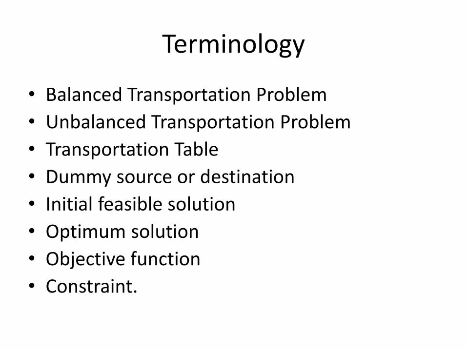
Steps in Solving the

Transportation Problem

Warehouse

Source W1 W2 W3 W4 Supply

Capacity

F1 30 25 40 20 100

F2 29 26 35 40 250

F3 31 33 37 30 150

Demand 90 160 200 50 N = Total supply/ Demand

Transportation Table

Special Issues in the Transportation Model

• Demand not equal to supply

– Called ‘unbalanced’ problem

– Add dummy source if demand > supply

– Add dummy destination if supply > demand

There are three basic methods:

1. Minimum Cost Method

2. Northwest Corner Method

3. Vogel’s Method

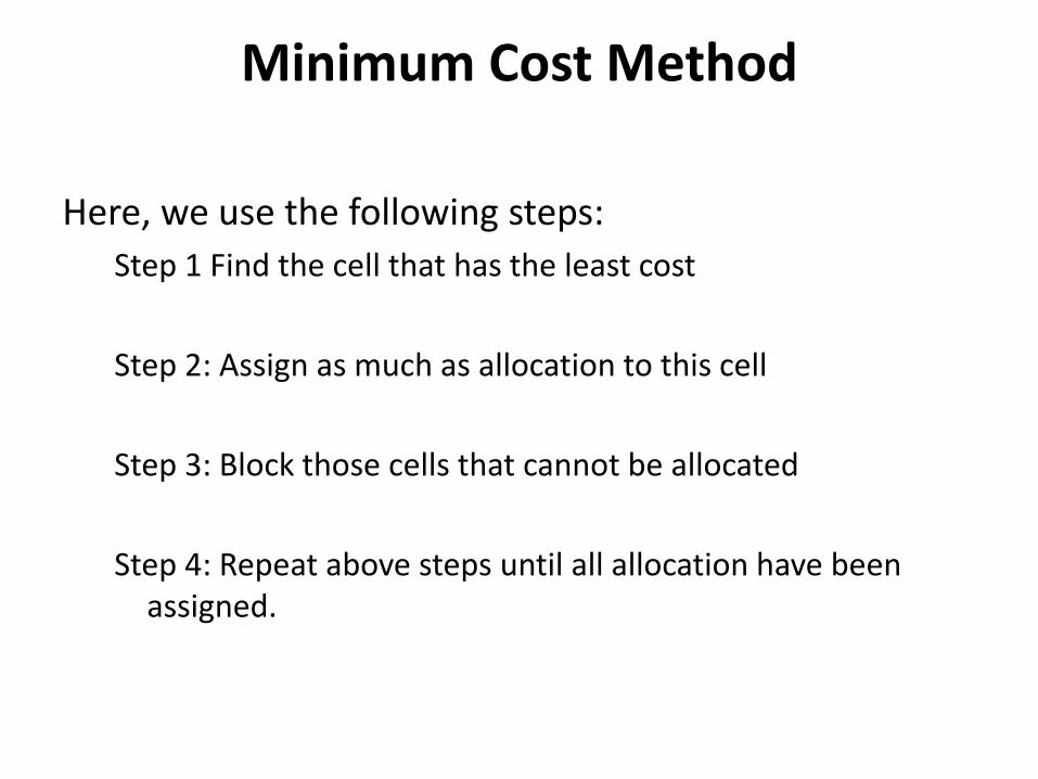
Minimum Cost Method

Here, we use the following steps:

Step 1 Find the cell that has the least cost

Step 2: Assign as much as allocation to this cell

Step 3: Block those cells that cannot be allocated

Step 4: Repeat above steps until all allocation have been assigned.

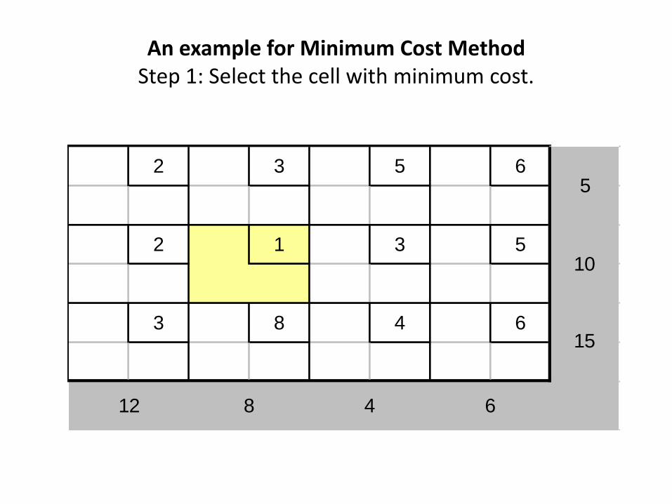
An example for Minimum Cost MethodStep 1: Select the cell with minimum cost.

2 3 5 6

2 1 3 5

3 8 4 6

5

10

15

12 8 4 6

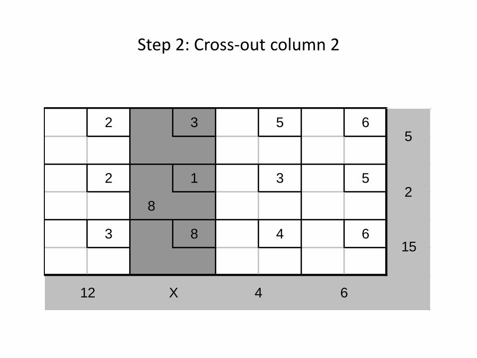
Step 2: Cross-out column 2

2 3 5 6

2 1 3 5

8

3 8 4 6

12 X 4 6

5

2

15

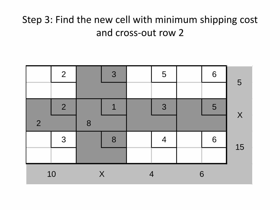
Step 3: Find the new cell with minimum shipping cost and cross-out row 2

2 3 5 6

2 1 3 5

2 8

3 8 4 6

5

X

15

10 X 4 6

Step 4: Find the new cell with minimum shipping cost and cross-out row 1

2 3 5 6

5

2 1 3 5

2 8

3 8 4 6

X

X

15

5 X 4 6

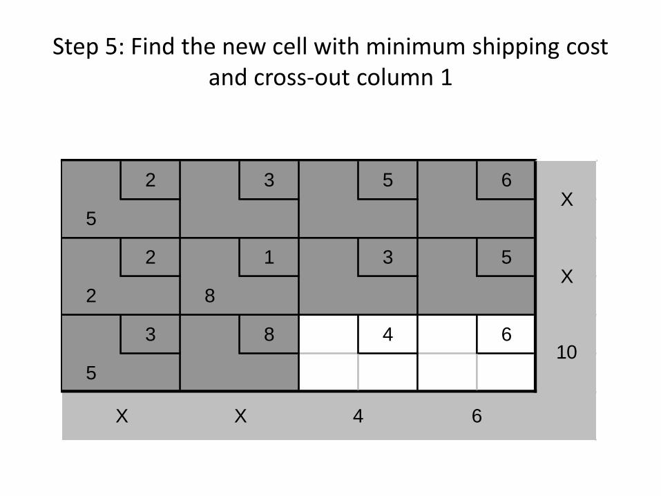
Step 5: Find the new cell with minimum shipping cost and cross-out column 1

2 3 5 6

5

2 1 3 5

2 8

3 8 4 6

5

X

X

10

X X 4 6

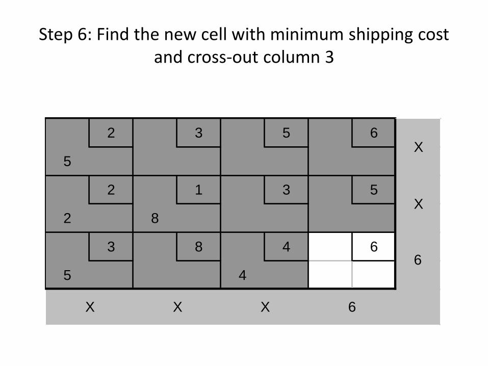
Step 6: Find the new cell with minimum shipping cost and cross-out column 3

2 3 5 6

5

2 1 3 5

2 8

3 8 4 6

5 4

X

X

6

X X X 6

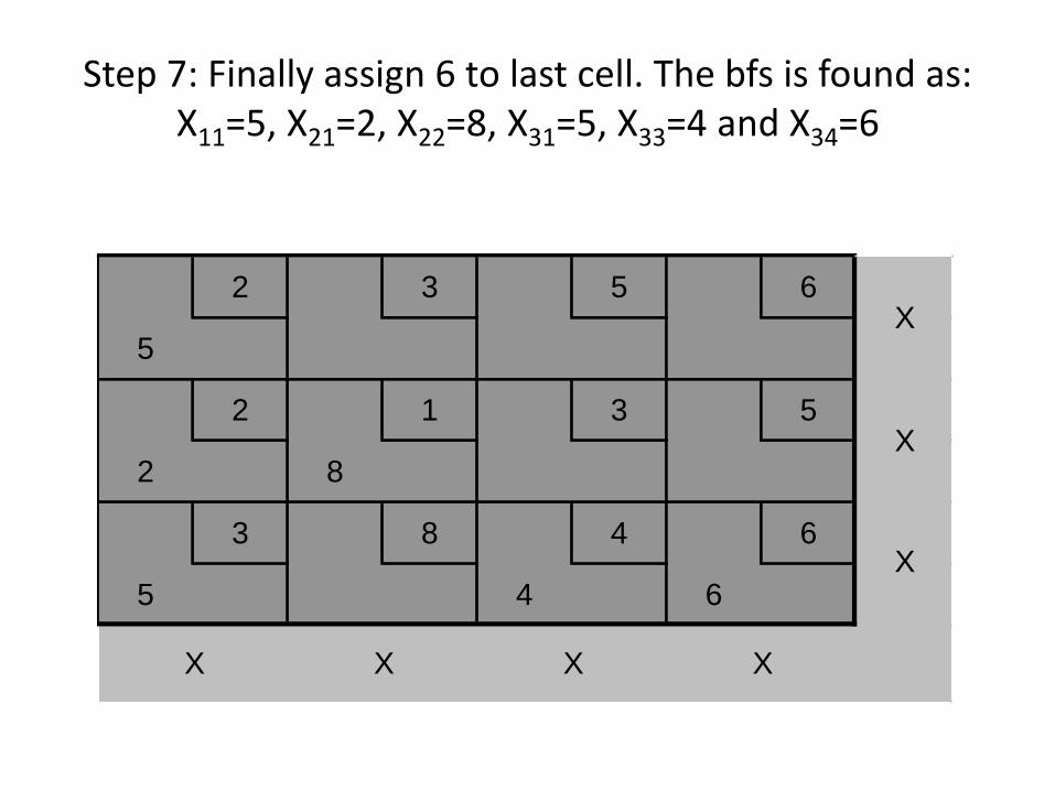
Step 7: Finally assign 6 to last cell. The bfs is found as: X11=5, X21=2, X22=8, X31=5, X33=4 and X34=6

2 3 5 6

5

2 1 3 5

2 8

3 8 4 6

5 4 6

X

X

X

X X X X

Northwest corner method

Steps:

1. Assign largest possible allocation to the cell in the upper left-hand corner of the table

2. Repeat step 1 until all allocations have been assigned

3. Stop. Initial tableau is obtained

18

Vogel’s Approximation Method

• 1. Determine the penalty cost for each row andcolumn.

• 2. Select the row or column with the highestpenalty cost.

• 3. Allocate as much as possible to the feasiblecell with the lowest transportation cost in the rowor column with the highest penalty cost.

• 4. Repeat steps 1, 2, and 3 until all requirementshave been met.

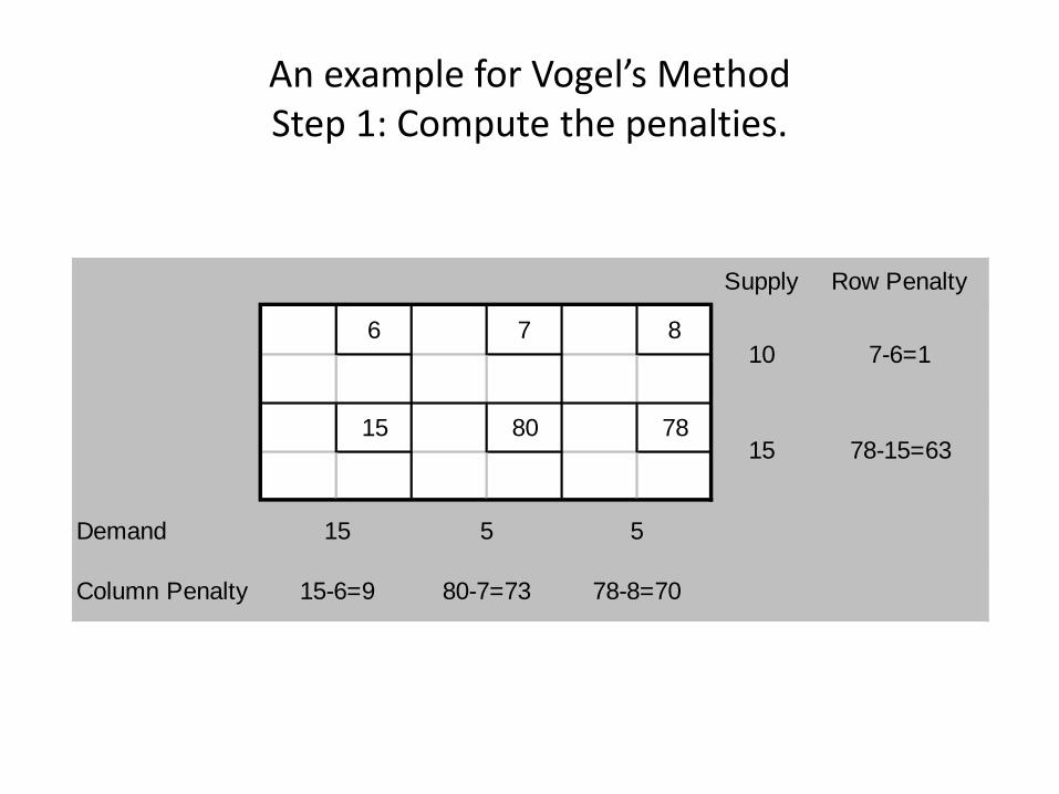
An example for Vogel’s MethodStep 1: Compute the penalties.

Supply Row Penalty

6 7 8

15 80 78

Demand

Column Penalty 15-6=9 80-7=73 78-8=70

7-6=1

78-15=63

15 5 5

10

15

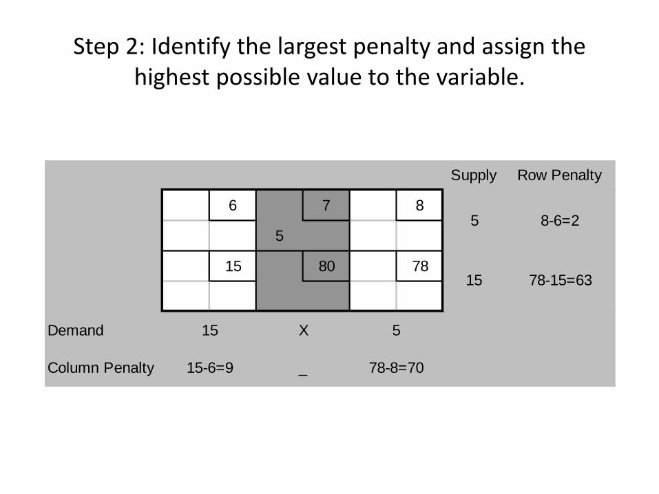
Step 2: Identify the largest penalty and assign the highest possible value to the variable.

Supply Row Penalty

6 7 8

5

15 80 78

Demand

Column Penalty 15-6=9 _ 78-8=70

8-6=2

78-15=63

15 X 5

5

15

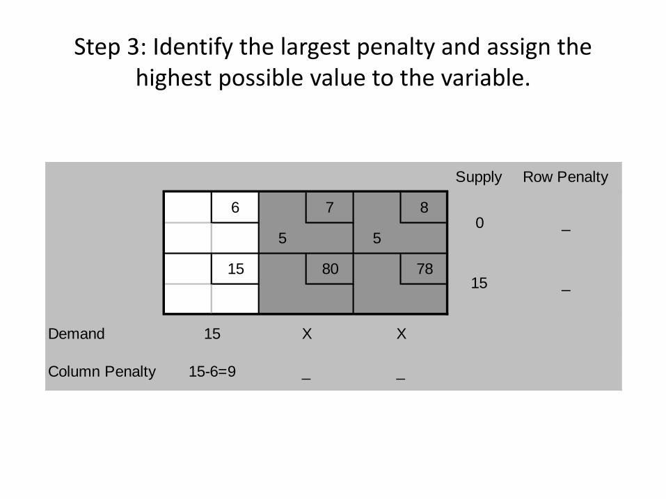
Step 3: Identify the largest penalty and assign the highest possible value to the variable.

Supply Row Penalty

6 7 8

5 5

15 80 78

Demand

Column Penalty 15-6=9 _ _

_

_

15 X X

0

15

Step 5: Finally the bfs is found as X11=0, X12=5, X13=5, and X21=15

Supply Row Penalty

6 7 8

0 5 5

15 80 78

15

Demand

Column Penalty _ _ _

_

_

X X X

X

X

Applications of Transportation Model

• Scheduling airlines, including both planes and crew• Deciding the appropriate place to site new facilities

such as a warehouse, factory or fire station

• Managing the flow of water from reservoirs

• Identifying possible future development paths for parts of the telecommunications industry

• Establishing the information needs and appropriate systems to supply them within the health service

2 February 2015

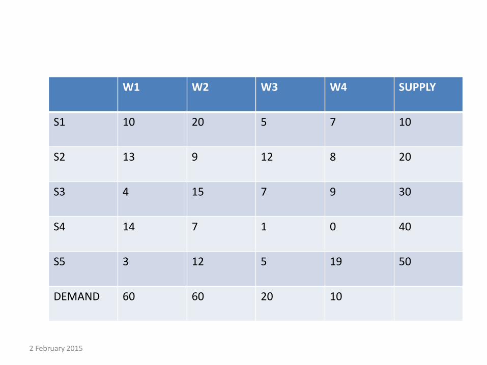
W1 W2 W3 W4 SUPPLY

S1 10 20 5 7 10

S2 13 9 12 8 20

S3 4 15 7 9 30

S4 14 7 1 0 40

S5 3 12 5 19 50

DEMAND 60 60 20 10

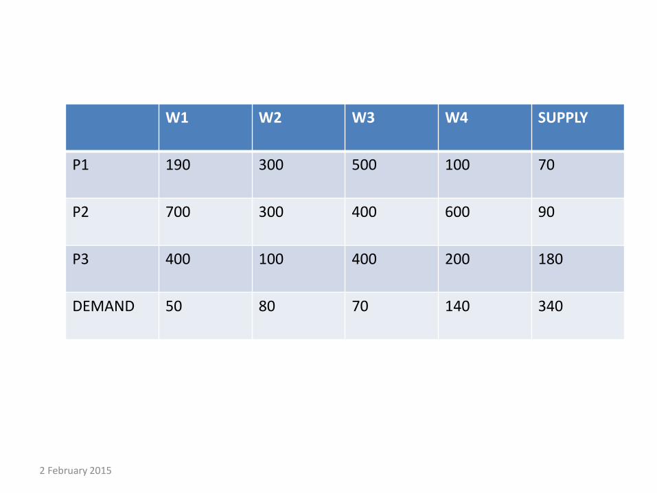
W1 W2 W3 W4 SUPPLY

P1 190 300 500 100 70

P2 700 300 400 600 90

P3 400 100 400 200 180

DEMAND 50 80 70 140 340

2 February 2015