TRANSPORT THEORY AND ADVANCED REACTOR ...

IAEA-TECDOC-254

TRANSPORT THEORYAND

ADVANCED REACTOR CALCULATIONS

FINAL REPORT OF THE SIX-YEARCO-ORDINATED RESEARCH PROGRAMME

BY THEINTERNATIONAL ATOMIC ENERGY AGENCY

A TECHNICAL DOCUMENT ISSUED BY THEINTERNATIONAL ATOMIC ENERGY AGENCY, VIENNA, 1981

TRANSPORT THEORY AND ADVANCED REACTOR CALCULATIONSIAEA, VIENNA, 1981

Reproduced by the IAEA in AustriaOctober 1981

PLEASE BE AWARE THATALL OF THE MISSING PAGES IN THIS DOCUMENT

WERE ORIGINALLY BLANK

The IAEA does not maintain stocks of reports in this series. However,microfiche copies of these reports can be obtained from

INIS Microfiche ClearinghouseInternational Atomic Energy AgencyWagramerstrasse 5P.O. Box 100A-1400 Vienna, Austria

on prepayment of Austrian Schillings 25.50 or against one IAEA microficheservice coupon to the value of US $2.00.

FOREWORD

The final report presented here on "Transport Theory and AdvancedReactor Calculations" concludes a Coordinated Research Programme (CRP)which was initiated and supported by the IAEA, and which has been carriedout by distinguished scientists in ten member countries.

Three main areas of reactor physics analysis were selected for theCRPî finite difference methods, integral transport theory methods andapproximate expansion methods» Within these areas the work was concen-trated on the improvement of accuracy, convergence and stability ofexisting methods, development of new methods and the application of theneutron transport theory methods for reactor calculations in practicalcases.

During the first three years of the coordinated research programmemany interesting fast transport methods were developed for calculatingthe neutron flux distribution in the reactor cells and core for one-dimensional symmetry; i.e., slab, spherical or cylindrical geometry.These methods were evaluated using the benchmark problems defined bythe participants. The methods were considerably improved in accuracyand rate of convergence and some important mathematical advances inthese areas were reported. During the final period the investigationsof the participants were oriented more towards practical 2D and 3Dtransport methods. Developments of 2D and 3D diffusion methods werealso included in the programme. A number of new ideas and methods inthe field of integral and integro—differential transport theory werepresented and discussed. New multigroup ID and 2D surface currentmethods were submitted as well.

In the field of diffusion theory interest was concentrated not onlytowards multi-dimensional finite difference methods, but also to the veryefficient "finite element" and "nodal" methods« Much progress was madein improving the rate of convergence of these methods and some applica-tion to reactor dynamics was reported. Applications of neutron transporttheory in the field of inertial confinement type of thermonuclear reactorsand associated plasma physics aspects were added to the programme of in-vestigations .

The final report begins with an introduction and is followed bychapters on Fundamentals of Transport Theory; Advances in IterativeMethods; Integral Transport Methods; Integro-Differential TransportApproaches; Finite Element and Nodal Methods in Diffusion; ReactorDynamics Calculations; Benchmark Problems; and Other Applications.There was no attempt to give a complete state-of-art picture of thefield and the report contains essentially only the results, obtainedby each of the individual participants of the CRP. Consequently, thechapters of the report were written by different authors and an attemptwas made to maintain a consistent style and for most throughout.

CONTENTS

Introduction ........<.........«........................................ 7Fundamentals of Transport Theory ....................................... 11

M. Boryszewicz , J. P.op-Jordanov.Advances in Iteractive Methods ......................................... 57

B. Beauwens , J. Arkuszewski, M. BoryszewicaIntegral Transport Methods ............................................. 99

V. Boffi , P. Benoist, A. Kavenoky, J. Ligou, J. Pop-JordanovIntgro-Differential Transport Approaches ............................... 177

J. Stepanek , J. Arkuszewski, V. Boffi, M. V. Matausek.Finite Elements and Nodal Methods in Diffusion ......................... 253

D.M. Davierwalla , C. Maeder, P. Schmidt«Reactor Dynamics Calculations .......................................... 273

J. Devooght t T. Lefvert, J. Stankiewiez.Benchmark Problems ..................................................... 305

A. Kavenoky , J. Stepanek, P. Schmidt.Other Applications ..................................................... 325

J. Ligou, P. Benoist, V. Boffi, B. Stenic.

INTRODUCTION

J. MIKA, V. CHERNYSHEV

Numerical methods for solving the neutron transport equation, thestarting point in the design of nuclear reactor systems, have been vigorouslydeveloped since the early days of reactor technology and have become in-creasingly important with the increased sophistication of reactor systemsand computing devices. At the same time, methods originally developed forneutron transport calculations are being applied to an ever greater varietyof problems connected with transport phenomena in other branches of physics.To speed up the development of transport theory methods in reactor technologyand other fields of physics and engineering among Member States the Inter-national Atomic Energy Agency sponsored the Coordinated Research Programmewhose activity in the years 1972-1979 is reviewed in this report. For theparticipating countries the programme was very useful in solving some oftheir everyday problems but it is hoped that the information disseminated sofar and included in this report will in addition be of value to the wholescientific community.

In January 1972, on the suggestion of the Coordinated Committee ofthe NPY (Norway - Poland - Yugoslavia) Project on Reactor Physics sponsoredby the IAEA in 1962-69, the IAEA organized the Seminar on Numerical ReactorCalculations, which provided an opportunity for reviewing the existingsituation with regard to numerical methods applied in solving the neutrontransport equation and the equations used for its approximation. The pro-gramme of the Seminar included five main topics:

(i) Transport theory methods(ii) Integral transport theory methods and applications(iii) Calculation techniques based on diffusion theory(iv) Synthesis methods and time-dependent problems(v) Developments in Monte Carlo.

The Seminar showed the great interest of scientists throughout theworld in reactor physics calculations with particular stress on methods basedon the transport equation.

A group of the seminar participants, discussing the need, suggestedthe organization of a Coordinated Research Programme (CRP) on Neutron TransportTheory intended to serve as a continuation of the NPY Project in a new formwith broader participation. The idea was supported by a group of leadingspecialists from five countries, namely Poland, Switzerland, Yugoslavia,Italy and Prance. Subsequently four more countries joined the programme,namely Belgium, the Federal Republic of Germany, Sweden, and the Soviet Union.

The first meeting of the CRP, on Methods in Neutron Transport Theory,attended by five scientific teams, was held in December 1973 at Swierk, Poland.This meeting was mainly devoted to one-dimensional integer transport methods,integro-differential methods, other transport methods (such as CN, Monte Carlo,tensorial method), and diffusion approximation methods.

The second meeting of the CRP, attended by eight representatives ofscientific teams, was held in November 1975 in Bologna, Italy. During themeeting progress reports on the results of individual research were discussedand the first benchmark intercomparisons of methods and codes were carried out.To stress the importance of the CRP and its practical applications, theparticipants suggested that the title of the CRP be changed to "TransportTheory and Advanced Reactor Calculations". At the same time it was suggestedthat investigations in the following fields be added to the scientific scopeof the CRP:

(i) Reactor homogenization theory(ii) Multidimensional neutron diffusion calculations(iii) Reactor kinetics(iv) Burn-up calculations(v) Application of transport theory methods in other fields

(plasma, charged particles, etc.).

The second meeting of CRP took place immediately after the TechnicalCommittee (TC) Meeting on "Methods of Neutron Transport Theory in ReactorCalculations", held also in Bologna and attended by 71 participants from 17countries. At the TC meeting 31 papers covering the following two main topicswere discussed:

(a) Mathematical foundation of the neutron transport methods(b) Analytical and numerical approaches for solving transport equations.

Participants stressed the importance of improving the methods of neutrontransport theory for reactor calculations as well as encouraging multi-dimensional diffusion calculations.

At the third CRP meeting, held in June 1977 in Paris, progress reportson the individual research and mutual cooperation were presented, the resultsof the second benchmark intercomparison were evaluated, and future directionsof activities in the frame of the CRP were discussed. This meeting maderecommendations concerning the organization of the TC meeting on HomogenizationMethods in Reactor Physics.

The various contributions to the CRP were considered in seven maingroups of topics:

(i) Transport theory(ii) Integral methods(iii) Multidimensional diffusion(iv) Iterative methods(v) Dynamic calculations

8

(vi) Applications to plasma and controlled fusion(vii) Calculation of benchmark problems.

The TO meeting on Homogenization Methods in Reactor Physics and thefourth meeting of the CRP were held jointly in Lugano, Switzerland, inNovember 19?8.

The homogenization methods in reactor physics are of consid«rablehelp, particularly in connection with multidimensional diffusion and transportcalculations in the task to increase computational speed and accuracy andcontribute to the improvement of reactor safety and give the possibility ofstudying much more accurately the fuel cycles which are important for reactoreconomy. All these problems were thoroughly discussed during the meetingat which 60 participants from 16 countries presented 33 papers.

At the fourth CRP meeting it was decided to finalize the scientificinvestigations within the framework of the CRP and to compile the mostimportant results of investigations and comparisons of benchmarks in a FinalReport of the CRP. The ultimate content and the shape of the Final Reportwere decided upon at the fifth CRP meeting held in Belgrade, Yugoslavia, inMay 1979.

The Final Report which is presented to the reader is, upon therecommendation of the fifth CRP meeting, a collection of scientific andpractical results obtained within the framework of the CRP during the 6 yearsof its existence. It is not the aim of the authors to give a well roundedmonograph devoted to a few aspects of transport theory and advanced reactorcalculations, but to demonstrate the variety of the problems tackled andsolved, sometimes only in part, by the CRP participants. There was no attemptto give a complete and up-to-date picture of the latest developments in thefield, and the report contains essentially only the results obtained by theparticipants.

An attempt was made to solve a number of problems by common effortalthough some were treated in only one country and then the results werecommunicated to the others.

The international cooperation induced by the CRP was not confined tojust the CRP meetings and the TO meetings organized by the IAEA on therecommendation of the CRP. A very important part of the activity was thebilateral contacts between countries participating in CRP which resulted incommon work and publications.

A particular feature of the transport theory and advanced reactorcalculations is that they offer a large variety of mathematical approachesand numerical methods which upon appropriate changes can be directly appliedin other fields. Chapter VIII of this report gives an account of some suchapplications executed among the participants of the CRP. It is hoped bythe authors that the report will contribute to a better exchange of information

between reactor physics and other fields of applications of the transporttheory methods.

It should be stressed that the transport theory by no means has reachedits final stage. There is still a need to improve old and to develop newmethods of solving the transport equation and its approximations in view ofgrowing requirements of reactor technology and related fields and the in-creasing sophistication of computers. The authors hope -that the results ofthe CRP presented in this report will not only be of some help to scientistsfrom other countries in solving the problems they encounter in their dailywork but will also contribute to a clearer picture of the future developmentof numerical methods in transport theory.

10

Chapter I

FUNDAMENTALS OF TRANSPORT THEORY

M. BORYSZEWICZ, J. POP-JORDANOV

i. BÎTRODUCTIONi'his chapter contains the results ox some ox the lundamental

problems encountered in reactor calculations, -xhe first partis devoted to the theory of approximate methods solving boundaryvalue problem ror the stationary neutron transport equation»It collects mainly the results of reserach carried at theComputing Center CJtPROHfik of the institute of Nuclear iiesearchat S"wi@rk, Poland by M.Borysiewicz, u.'.K.ulikowska, R.Stankiewiez,and G.bpiga from tac University of Bologna»

Tue second part is devoted to investigating tue neutronscattering kernel in thermalizauion and solving down problems.Tne work was done at the Belgrade University s Boris KidricInstitut« ana the faculty of Electrical engineering byD.otsfancvic, MBMarkovic and J«,Pop-Jordanov.

Section 'i.1 was prepared by M»Borysiev»icz and Sections1.2 and 1*3 by MsMarkovic, J.Pop-Jordanov, and i»«Ste|tanovic,

1.1. THEORY OP APPROXIMATE METHODS SOLVING BOUÏÏDARY VALUEPROBLEM FOR STATIONARY TRANSPORT EQUATION

1.1.1. IntroductionIn recent years many modern techniques solving boundary value

problems have been developed on basis of approximate variationalformulations. This is usually done in terms of bilinear formsbounded in certain functional spaces. This technique easilyprovides us with the so called a priori estimate, which implythe uniqueness of the weak solutions. At the same time it isa convenient tool for investigation of the order of convergenceof various approximate methods solving the original boundaryvalue problem.

11

In the papers [l] and [2] the theory of bilinear formssuitable for the neutron transport equation is developed. Thesebilinear forms are bounded with respect to both their arguments,each of them belonging to an approximate functional space. Ingeneral the spaces do not coincide. Moreover these bilinearforms are not coercive in standard sense. The authors of [l]and [2], making use of the a priori estimates, found theconvergence criteria for a wide class of promotional methods.

In Sec. 2 of the present chapter the concepts of [il and [2]are developed such that they may be applied to analysis of finitedifference and hybrid methods, the latter concerns nodal,response matrix or local Green's function techniques.

In Sec. 3 a general nonlinear variational problem is studiedunder assumptions which correspond to the neutron transportequation with the cross sections depending an the uknow solutionthrough the temperature feedback.

Section 4 provides a link between the general theory presentedin Sec. 2 and 3 and the boundary value problem for the neutrontransport equation.The relation of this theory with the basic mathematical problemof homogenization is also discussed.

It will be seen, from the results of Sec. 2 and 3 that thedetailed knowledge of the behaviour solutions to a given equationis prerequisite for any attempt to estimate the approximationand convergence rate of en algorithm solving this equation.The problem of smoothness of the solutions to the general 2-Dneutron transport equation is studied in Sec. 5.

1.1.2. Y/eak solutions a.nd approximate methods for the equationsrelated to noncoercive bilinear forms

Let and are two Hubert spaces such that 6 is a densesubspace of and

i 1UII 4 k 1MI zt12

Thus vie have(2) Be L c B* , Ic'MUil , 4lkl 4 k 1*1 >B* L o '

where B* is dual of B with the point space L . The norm in &*can be defined by the formula(3) IMB* - st£lkr*|0u,o-)| t wlth (*,„)

being the inner product on L-t .Consider the bilinear form a(-u,u-) with the property

(4) I * (<*.*) | 4 C*M IM.ti DWith the f orra a(/a, ir) we can associate the continuous linear

operator A from 5 into L by the relation

(5) ( A u , fr) = et (tt , t>) / • 0-6 & .

The domain of A is given byj

D(A)- | u • for each O-G& there exists fc <oo such that

I *(«,*) U k H

We assume that the bilinear from Ct(^,^} generates anotherform a*('U,u') such that(6) €»*(/«/ «>-)a aC'U/ir) for -u, ü- e ß ;

and(6a) a-

With the form a (it, o-) we can relate an operator A in similarway as A to 0( ,0-).

We require that ß-D(/\A) and A4 is a one-to-one transformationfrom B onto L . To ensure this property it is sufficient toassume A - A and

4

(7) Re a(<u,ii) £ Cal|<u!luIt is obvious that in this case

a(/u/y) - (11,

The Eq (7) can be considered as a generalized coercivzxesscondition for the form CL(AL,O-}.

^

With this assumption valid we can prove (j, 3] that for each Se 6there exists an unique solution of the generalized variational problem.

13

GVP. Find tt e L such that for each o-& B we have

Such a solutionna is called the weak solution of the equation(9) A>u = $

Consider.- two families of the spaces L and 6. . k ^ CA 4je h, n iWe define the approximate problem.AP. Pind ju e L such that for each Or e 6 we have

The set of assumptions concerning L and 0, relevant fork lfurther analysis we formulate asAssumption A

CV/ (V

(i) Por h,-*-0, Lfe and 6fe tend to L and ß , which denseIn L and B , respectively,

lii) There exists J^> 0 such that for h,e.ke the projection—^ *****

\ from L onto îs also a bisection of 1*^ onto L-^ ,where ^=A*Bk.

(iii) f = lim f > 0 , whereh-»o n

t = c»/11 X^W

Under Assumption A for the problem AP vie can prove thetheorem concerning the convergence of>u, to the solution it ofKthe problem GVP[j, 2"].Theorem 1« There exists a unique solution of AP for each h •

The sequence ^/Utl converges v/eakly to the solution 14 of GVP.If moreover L^= LK then the sequence {I K} converges in thenorm of L . The rate of convergence is determined by the bestapproximation of -u. by the elements of L^.Theorem 2. If

(i^ the solution to of GVP belongs to(ii) L K = B K c B(iii) condition (.7 ) is satisfied

then the solution -u^ of AP problems are convergent in L normto the solution /vt of GVP. The rate of convergence is given by

14

111) .n U

where It is the solution of•

(I1a) <*with e

for each

Now, we can consider more general case when B^ and Lâre not subspaces of B and Lt respectively. That is we have thesituation

OL

(12)

A

CL,

The operator A, is defined by the form cd ""1"') satisfyingthe properties (4} and (6) stated in terms of the spaces 6^ andL, . The operators p , b and 5U and I, make then I |r^ rï, »t n*"correspondence" among the elements of ß and B^ and Land L, , respectively. Under some additional compatabilityconditions for the operators p , b, and s^ , lh vie shallprove the generalizations of Theorems ("]} and .( 2 ) , stating thecriteria of convergence in the norm of L and L^spaces. Supposenow that a,^,^} is of the form

(13)

Consider the approximate problem.AP' Pind Uu Ê L, such that for each o- e 6, we have~ ~* n n n n

(14)

15

where the bilinear form a(/uk/ l} is defined by Eq ( 13 ) and

Formulate the analog of Assumption A..Assumption A*

5. L, and p B, are dense in the limit in L and B,H h. (H k 'respectively .

(ii) There exists hB}0 such that for H é h0 a projection T?i~*>

from L onto S L is also a bisection of L« K onto

(iii) ^ ~ liai f > 0 , where-? "

=- _Making use of the technique developed in L 1 » 2 J and ["4!

we can prove the theorem.Theorem 3. Under Assumption A' the results of Theorems 1 and2 can be extended to problem AP', in particular

(i) p u- converges weakly to the solution 4L of GVP;(u) if -^ then

(iii) if u € ß , L^= B^ and condition (6 ) is fulfiled, then

where û. is the solution of (11a) with

Theorems 1-2 form the mathematical basis to analyze a certainclass of approximate methods solving GVP. This class includesthe promotional methods, therefore the finite element methodswith approximating spaces L. and 6R satisfying interelement4continuity relations imposed by the properties of the solutionsto GVP. Theorem 3 is suitable for the standard finite differenceapproach to solve GVP. It should be noticed, that one can

16

considerably weaken the requirement of interelemant continuityfor the functions of &^ andLând still obtain a convergentmethod. One gets so called nonconforrning methods. They are basedon the extended variational formulation, often called hybrid, one,in which the continuity constraints are removed at the expenseof introducing new terms in the bilinear form. In the followingwe formulate the hybrid method related to the bilinear formssatisfying Eqs (4) and (6) in suitable functional spaces.

Suppose we have three Hubert spaces B , U and M .Let the bilinear form G.yU.to-} satisfy the conditions analogousto (4) and (6). Let finally Mtf-( n\ be a bilinear form on L x Msuch that the quantity ILu 11^ given by the equation:

is norm on .V/e define the hybrid variational problem.

HVP For given linear forms f (o-) and a if-} continuous on ßand M ! respectively ; find a pair (it, )e LxM such thatfor any (o-tu}&. ß x /"! wa have

K/-JIn similar way vie introduce the approximate problem

HAP in terras of approximate forms fa(^/^)/ Th.(°h) I Kand $h(/*h) continuous on L^x B^ , 6fe , 6^ x M^ and fl^respectively. V/e assume that the spaces ßfe , Lfe and ^fe aredense in the limit in the corresponding spaces ß , L and "

Following the reasoning of [j» ch.3] and [5 chap.l] wecan prove the existence and uniqueness of the pair (/a, fl-)e L x Mwhich solves HVP. If /(<>•)= (S, <r) with 5 e L, then thesolution ('U/k) belongs to B * M * The similar statement isvalid for a pair (uk, Ah ) being a solution of HAP.

17

Now vue estimate the error bounds for II 4i- -WH IL andTo do that we first define sets V, and Vfe k

for

(18)

If ( /t,/ ) ek/j/'1^) is a so u" 011 °f HAP» then IL. solvesthe problem.HAP' Find u^é V, ' such that for any ix 6 V,- n A n £

Lemma 1. Sufficient conditions for the existence of (>u (X, e ß x M.••— —— — —— » » h /(, .»v h / j^ h- the unique solution of HAP are:W K=\5_

(19) Ui) the form ä (itî^) satisfies Eqs (4) and (?)}ia a norm on ^ > where

The proof of the lemma are based on that given in ["5, chap,modified in such a way that the generalized coercivnesa condition(?) may be taken into account , [^4J»

The estimation of error bounds found in [4"] for HAPare summarized in the following two theorems.Theorem 4. Suppose that the assumptions of Lemma 1 are fulfiled,then there exists a unique solution nji 6 B^ of HAP.' The error

ll/iL-/Ukll- where u. is the solution of HVP, can be estimated asfollows:

E 4 C\ inf,L l

(20)

18

Theorem 5« We assume that the conditions of lemma 1 arefulfiled. Then there exists a unique solution (uh, ) of HAP.Basudes of estimation of JI/u-/uKH- stated in Theorem 4 we havefor II*-*J'

The erro bounds for lU-aiJI^ i* Theorem 4 and a fortiorithat of Theorem 5 for 1IA-%K!IM involve the quantity

Or »Jj .(22) 4 /l

Hith 0^6În practice^to estimate (f( ) we must know interpolation

properties of V^ with respect to a subset of & witch thesolution belongs to. The following theorem permits us toavoid such an inconvenience [[4].Theorem 6. Under the assumptions of Lemma 1 we have

(23)

Uovs we shall give an example how to relate H\TP to GVP.Suppose that the domain of the definition of functions beingelements of the Hubert spaces 6 and L used to formulate GVPis a convex set G in an Eucliden space. To denote that we

19

can write G> = B[G ) and L=L(u) . We can décompose G( intodisjoint sets G^ L=1,2)...,1^ , such that

124) G =

We introduce the product Hubert spacesn

(25) B = T T 6 ( G L ) and L = T T L ( ß t ) .

If the operator A related to the bilinear form at

continuous in L(G)*B(G) is an integrodiff erential one, thenany linear functional on B which vanishes on anyo-€ß(fi)can berepresented in terms of a bilinear form bfa/u) continuous inß x M , that is

(26) Ç

where ' / is a suitable chosen Hubert space of functions definedn

on .U 9 G- , where 'SG- ±a boundary of G j .In this case thehybrid variational problem HVP whose unique solution is aiaothe solution of GYP can be defined by means of the forms b( **//*)and dC^/i*"/ , where(27) ä ( ,0-) = 2 a-(<u,i>-)v ' L=l

The formal definition of <at; (up] in L (&i) x B(G^) j_a .ê sanieas the form OLô} of GVB in L (£) x 5(G ) .

It should be notea tnat results of this section can begeneralized to the case when ]_ andßare reflexive Banachspaces.

1.1.3« QuasilJnear problem

Suppose that the form OL(U,I>} is continuous in L, x 6 butnot necessarily bilinear. It generates, in general, a nonlinearoperator A from P(A) c ß into U . For simplicaty we can assumethat D(A")=& . In the following we analyze a certain class ofapproximating methods solving GVP when the form of(/",f) satisfiesEqs (4) and (7 ).

20

Pirst to simplify notations v»e define '^(^L,k}>t(S,£jandby the equations

(23) y

and

(29)

(30)

Where the operators p and {, are those of the diagram ( 12).The functions y(/U,A) and i($,<->k} can be considered as errorsof approximation of the form OL(Û,I>) by ah f'W/,/ ) a^d "th6 ^ $k'How we formulate the set of conditions which can be consideredas an extension of the stability conditions introduced by Aubin£6j.

Condition 5For any £>£? there exists £>#such that

(_SÄ) For any £>O there exists /?>£> such that

Moreover it is required that for any K >0 there existssuch that

(31) IUJ1 > •H

Lemma 2 If A and /Aâre surjections and U^^ are solutions ofGVP and AVP respectively then

The statement of the leuraa follows directly from the definitionsof GVP, AVP, ^(-W,/»J and i(Sf^j . Making use of the resultsof Lemma 2 and Condition 5 -we c#n..p:eove the theorem.

21

Theorem 7 If (51) or(#a) of Condition S is fulfiled and

then

If the operators ^ and £fc satisfy the followingstability criterion

(32) C any

and the convergence criterion

(33)

then under the assumptions of Theorem 7 we have also

Hs./u, - it'll — * 0, .(34) ,Lwhere 'ii and 4L, are solutions of GVP and AVP respectively.n.

Conditions S is fulfiled if (•«/,/ / is bilinear in ß>h* "and it is coercive in ^ k in the sense of Eq (7). How we shallgive a non trivial example of application of Theorem 7 toa nonlinear problem.

Suppose we have the forms

(35) OL(M,O) - 6( , ;y) and Ct^fa, <£ )=

where

(36)

We assume that the similar conditions satisfies , tt^'U.. Inthis case from the definition of < it follows

-* * "H

22

If 4À, is a solution of AVP thenn.

I»)

Thus the requirement

imposes restrictions on || 5 II • In i'ac't we admit £>. for which(Lthe LH norm of the solution 11^ can be estimated as follows

(39) IUJU pwhere p is such that

(40) 6 - ~~cf~~ < 4

For such & Condition S is satisfied and we can applyTheorem 7 to conclude

provided ^>^,k}-^0 and £ (2, 5J — ' 0 .In our case AVP is itself nonlinear and we must

propose an algorithm to solve it. To do that we considera sequence of linear AVP.Find /U* such thatk

(42) b„ K"? < ; ï ) = ( *v <ï ) • ror " ï e 6*From the assumptions on é>, (u,. .41, ;& } we obtain the estimation R] •fi* n i h. l n. '

n.(43) h

where «U is the solution of GVP.If

(44)

23

then from Eq (_43 ) vie have

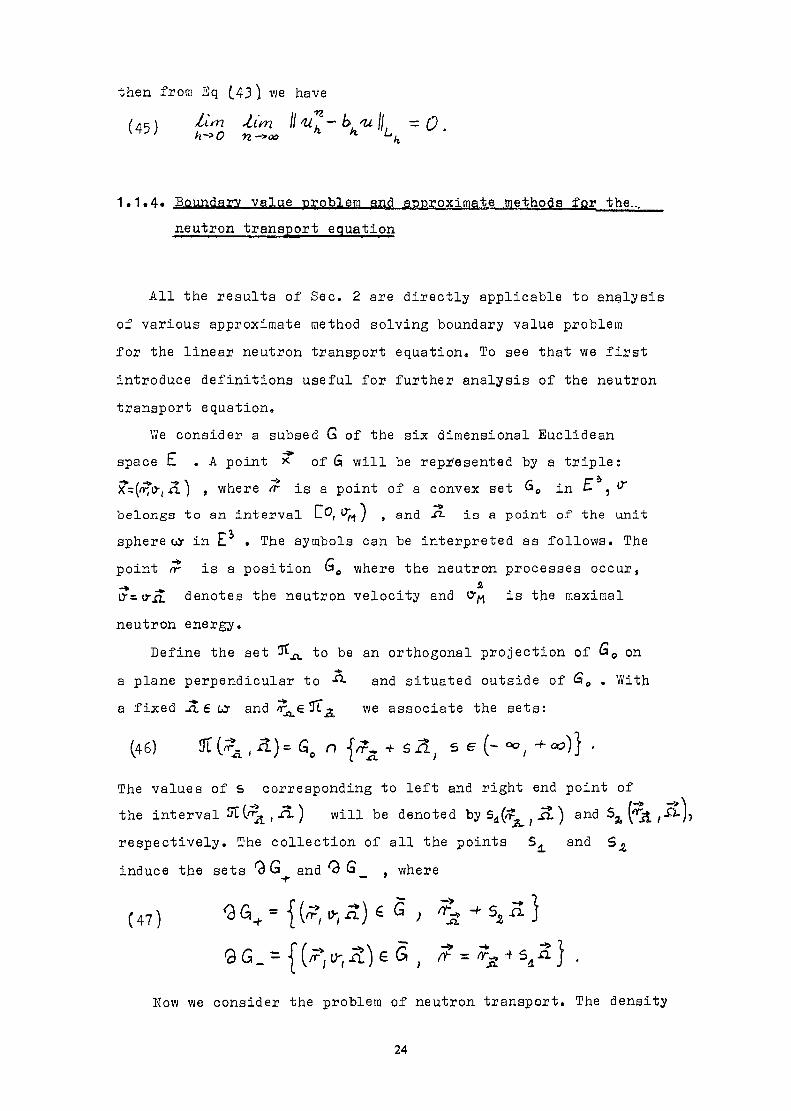
1.1.4» Boundary Vfllue problem and apprgxiggte methods for the,neutron transport equation

All the results of Sec. 2 are directly applicable to analysisof various approximate method solving boundary value problemfor the linear neutron transport equation. To see that vie firstintroduce definitions useful for further analysis of the neutrontransport equation.

V/e consider a subsed G of the six dimensional Euclideanspace £ . A point * of G will be represented by a triple:>T=(ff j-( a. ~] , where ^ is a point of a convex set 60 in £ }

t?*belongs to an interval L®, ) , and -fi- is a point of the unit

Ei . The symbols can be interpreted as follows. Thepoint (r is a position 00 where the neutron processes occur,-» ao-=i>-£L denotes the neutron velocity and o-M is the maximalneutron energy.

Define the set t&st_ to be an orthogonal projection of «0 ona plane perpendicular to -0- and situated outside of G0 . With

^ - j*»a fixed ,a 6 ccr and /r 6 -T L . we associate the sets:

(46) 3r^,Ä)«60 nThe values of s corresponding to left and right end point ofthe interval 0^ , A) will be denoted by Sd (o^ ; jrl ) and Sarespectively. The collection of all the points 5^ and S

induce the sets G and 0 G_ , where

(47)

9 G_ = ;,.£)£ GNow we consider the problem of neutron transport. The density

24

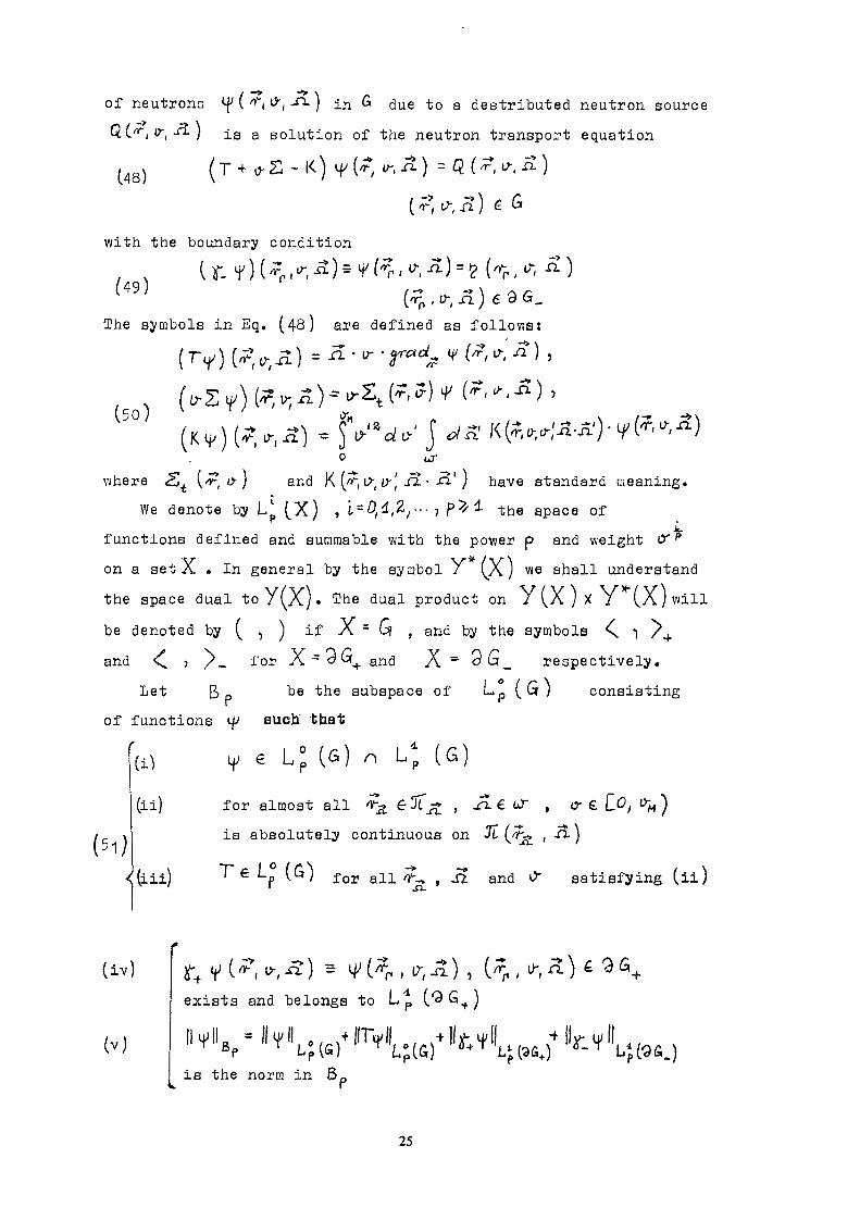
of neutrons ^ ( ""i &, -"- ) in û due to a destributed neutron source, w, -^ } is a solution of the neutron transport equation

(43)

with the boundary condition

(49)The symbols in Eq. (48) are defined as follows:

, ,(50)

(KH «

= î ' ^ jwhere <St (/r, tr ) and K (/?", i ( y- ,' -/î - -^ ' / hâve standard meaning.

We denote by L^ (X) , 1 = 0,4,2,... , p^l the space offunctions defined and summa blé with the power p and weight i>" p

on a set X . In general by the symbol 7 (X) we shall understandthe space dual to Y(X) • The dual product on Y (X ) X Y (.Xjwillbe denoted by ( , ) if X = G , and by the symbols S l Xfand ^ ? /_ for A. ~ & + and A = o «_ respectively»

Let B - be the subspace of Lp (6) consistingof functions if auch that

(i)(ii)fcii)

€ LJ (G) (6)for almost all ^ ë-^JÎ » -^ € <*is absolutely continuous on JI (

all , -ft and

o- £

satisfying (ii)

(iv)

(v)

exists and belongs to L p

is the norm in

25

The properties of ß„ have been extensively studie-d in L il •Aa

In[l] and [2] it is proved that the operator A = (J+ 0"Z - K)x ^+is bisection from E> onto L =Lp(G)x Lp(Q&_) provided zerodoes not belong to the spectrum of A - T •*" D'2 ~ K with

*** f,

DCA) = ß p = ^ i f e ß p J ^ - y = O J . Moreover we have

(-52) UA'1! _^ 4 C i «o

Similar conclusions are valid for the operatorA* - (-J + &•£ - K^jxtf-

In the theorems ensuring (52) presented in £1 ] and [2Jsingular slowing down kernels and ^ns °° were admitted.

Define the form et (il, y } bilinear on L> x ô by theformula

(53)

where

Take {Q,^j £ 5* then by the results of [1~] there existsa unique solution "t£ - { if , i^ j of GVP defined by Eq. (8 )with

(53a)

.Par -IX. we have

(54) I K f , p

where c is the constant of Eq. (49). If Q,]&L then

(55)

26

It should be noted that a (-a, if) defined by Eq. (50) iscoercive in L»a - La \G ) x L2 ( G ) if the following conditionis satisfied

(56)Similar results are valid for the GVP related to the form

-K)

It is easy to see that there is the complete correspondenceamong the spaces Brt and L " , used in the definition of GVP> "ifor the neutron transport equation, and the spaces B and Lfrom Sece 2 and 3 where the general theory of approximate methodsis presented. Therefore all the estimations of error boundsstated in Theorems 1 and 3 are valid for promotional andfinite difference méthodes solving boundary value problem for theneutron transport equation. In particular they are applicable to

(i) spherical harmonics method,(ii) finite element method,(iii) general Bubnov-Galerkua method.Suppose that the set GO of position vectors ^ is partitioned

into G^ j £=4... /^/disjoint subrogions with the boundaries 9G-

(57) G*'âG;The form b(it;/w) bilinear on 6x M suitable for HVQ for the

neutron transport equation is defined as follows

(58) b KA) -2 (<*r. Nwhere r ^ •% , — \ a i r \& f n 6p (G.J j

isd

In similar way we define bh(/w, , /<A) > B, and M^ .The elements of Bp (GL) , L° (9 G .) and L°('9G_) can

be interpreted as .the. neutron distribution in G. ,outcoming and incoming partial interface currents respective-ly.

27

With b(>Ur/a) defined by Eq. (58) and the b'ilinear form,tr) generated from Ct (u,*) given by Eq. ( 53 ) , according

to the recipe of Sec. 3 we can analygs in frame of HVP thefollowing approximate methods solving the neutron transportequation -

(.i) variational formulation with discontinuous in space.,variable trial and weight functions,

(ii) partial boundary current method,(iii)response matrix method,(iv) local Green function method.Consider now a family of forms & (it, w) defined by Eq.(53)

with the cross section 2 = <E!H and" the kernel of K - KH dependingon a parameter HÔ. We assume tfcat Eq.(56)is valid with f such that

(59)

We shall denote by ao (u^ the bilinear form defined in termsof20 and K0 being limits of £H and KH for H-*0 . Now vieformulate two theorems relating the solution of two followingvariational problems (?"] .

For given 5H={oH , <?H } € LA- findsuch that for any LT € 6 s B v'e have

(60)

GVP

For given 50 £ LZ_ find /MO £ LZ such that for any15-e ß we have

(61)Theorem 7 Assume

28

(ii) there exists an operator P and an integer 1?.0 such

that (T'* ~P/ » '?2>??fl is compact from L. into L,,, (G)and

(?(T-*?)>^)>CpM , ye** *•

thenH/"H-'OI, — * 0 .

»-2,4

Theorem 8 Suppose that(i) 2JH—>20 weakly in L £ ( O )

5U —> £ weakly in L0ri o & •~

(ii) for any </> 6 L ,£ ( G ) we have K H If = K

with the operator P bounded in L£(G) such that "P =Pand the set "P 5^ is compact in L^ (G) then 1113 (if-a») || ""ri-to*

L-alS)where «j; and u; are the solutions of GVP„ and GVP .Trt »o n 0respectively.

Both Theorems 7 and 8 can be considered to be basic forthe general theory of homogenization for the neutron transportequation. They correspond to -those proved by Babuska £. 11J forthe diffusion equation.

In the concluding part of this section we examine the formof the transport equation which includes the second orderdifferential operator with respect to £ . The operator, underan additional assumption is selfadjoint and positive definite.This case was extensively studied in literature L12-18 J. Forsuch an equation the appropriate functional can be expressedin terms of the norm generateâ by the selfadjoint extensionof that positive definite operator. The rigorous treatment ofsuch a problem for the one-velocity tra'nsport equation withzero boundary conditions-and even parity scattering kernel canbe found in Cl2l . The requirement of the even parity wias rela-;a»d in the recent paper of Kaper at al j.16 J • he autjaeaftuse the Friedrich's approach to extend a positive definiteoperator. They minimize an appropriate functional over a Hilbertspace v/hich is, in fact, the domain of the extended operator.

29

However the trace theorem for the space considered is based onthe assumption that. for any convex body the .chord. measured alongjnis always bounded away from zero. This assumption is hardlymet in practical applications.

Recently Pitkaranta {j8j considered variational formulationsfor the multigroup transport equation with homogeneous boundaryconditions» The author also assumed that the inter-group transferkernels are symmetric with respect .toK. dependence. In thepaper \_2~\ the problem of the transformation of the transportequation to the second order form . are examined under theassumptions which cover all the practical situations. The authorstook into account the continuous dependence of the neutrondistribution of the energy, whose interval may be infinite. Thenonhomogene ous boundary conditions and arbitrary scattering andfisaion kernels were admitted.

We define projectors P1 and P2

By K and KQ we denote the operators

(63) Kaf eTaK fWith the operators K and K we associate two operators H and*^ 9 8H by the formulas:

(64) Ha{ 5The transport equation is now the following pair of coupledequation

(65) T/it^ï H s^6 = Qs

and

In [2l it was proved that the operator Ha is linear boundedtransfomation of La (ja) onto L/(GV Moreover the inverse Haexists and is bounded in all the situation of practical interest.

30

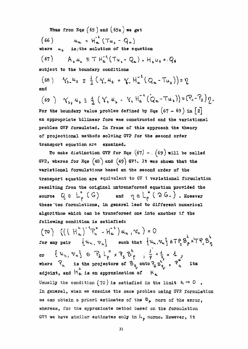
Thus from Eqs (65 ) and (65a) v»e get

(66) ^ -- V C C T X - QOwhere /w.6 Is y the solution of the equation

(67) A b -u s 5TH;HTu f c -subject to the boundary conditions

(68) Y*J*s =and

- iFor the boundary value problem defined by Eqs (67 - 69j in [2jan appropriate bilinear form was constructed and the variationalproblem GVF formulated. In frame of this approach the theoryof projectional methods solving GVF for the second ordertransport equation are examined.

To make distinction GVP for Eqs (6?) - . (69) will be calledGV2, wheras for Eqs (48 ") and (49") 6V1. It was shown that thevariational formulations based an the second order of thetransport equation are equivalent to GV 1 variational formulationresulting from the original untransformed equation provided thesource Cj G L_ C G) and >o 6 Lp ( *a G- ) . Howeverr rthese'two formulations, in general lead to different numericalalgorithms which can be transformed one into another if thefollowing condition is satisfied)f 70^ f f ( H* l T* - V-T )>u.u 1=0\ I V \ v I * *\ / \A * * QJ / n i ** /%. J \ ^ "W / ™ * ^^ r * t I

A _ f 0 ^^* fN ^^for any pair 1*K, ^1 such that i^v^KA 6' % "^pU ' r»-j v J J I1. » *

fe or t u ' H )y v ^ 5 C r i 2 1 i - ) < T 1 D ^ , ) f t s •*• ^

where *?^ is the projectors of *%>„ onto?,,ß , ^. its. t\ > Vadjoint, and H^ is an approximation of HÛsually the condition (?o) is satisfied in the limit k -» 0 .In general, when we examine the same problem using GV2 formulationwe can obtain a priori estimates of the Bp norm of the error,whereas, for the approximate method based on the formulationGV1 we have similar estimates only in L norms. However, it

31

should be emphasized that GV2 provides only the even componentof the solution. To calculate the odd component vie use therelation Ü66 1 and consequently we get again only Lp estimationof the error for the entire approximate solution. It seems thatboth approaches are completely equivalent from the point -ofview of approximation theory.

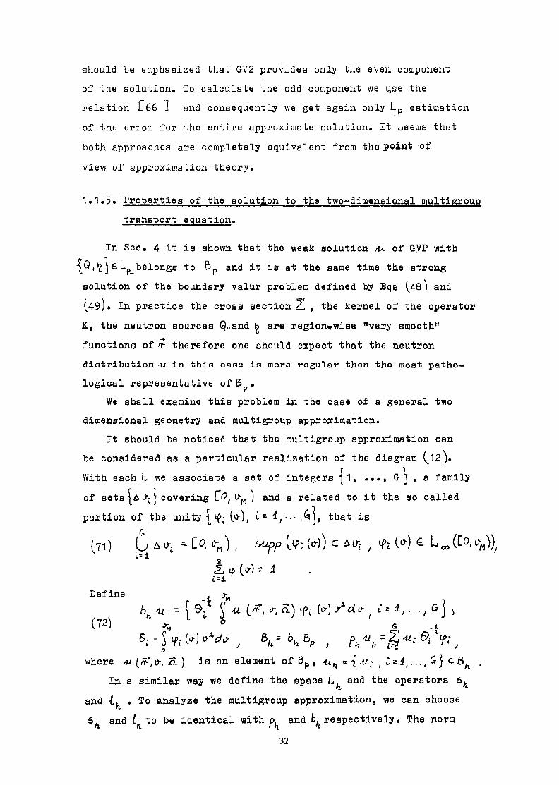
1.1.5. Properties of the eolation to the two-dimensional multigrouptransport equation.

In Sec. 4 it is shown that the weak solution /u. of GVP withQ<Ï J fcLp_ belongs to Bp and it is at the same time the strongsolution of the boundary valur problem defined by Eqs (,48) and( 49)» In practice the cross section 2 , the kernel of the operatorK, the neutron sources fyand £ are régionalise "very smooth"functions of or therefore one should expect that the neutrondistribution u. in this case is more regular then the most patho-logical representative of E> .

We shall examine this problem in the case of a general twodimensional geometry and multigroup approximation.

It should be noticed that the multigroup approximation canbe considered as a particular realization of the diagram ( 12).With each k we associate a set of integers |1, ..., G j , a familyof sets|&tf-j covering C^ o-^j and a related to it the so calledpartion of the unity [ if : (o-), t= 4,... (£j, that is

(71) U A*^c-1

Define

(72) s

«here /u ((£,0-, A ) is an element of Bp , <un = {/«; , £ = 4, ..., S j c 6In a similar way we define the space L and the operators 5

and I. . To analyze the multigroup approximation, we can chooseS^ and f, to be identical with p and ^respectively. The norm

32

nX=bftX . Where X is one of the spacesß L is chosen to be

(73) 'KII

It is easy to check from Eqs (53), and (?1 - 73} that thebilinear form (J 3) generate s the boundary value problem formultigroup transport equation. Now the operators T, 2 and K

t*>^r <"*w

from Eq. (^47) can beiiidentified with GxG matrix operator T ,2»s» r*s l~" ~^

and K where T - t>, T b, and 21 and K are defined inn- h,e similar way. Sime our choice of operators b, and p impliesthe stable and convergent approximation of Lp(CO, uv)) specesE 6 ] then the condition of Assumption A'are satisfied and wecan apply Theorem 3 to the multigroup approximation defined byEqs (71) -(73). In our case the set of functions {cp (v-) ,l = 4.r..lG\ describe fine structure of the neutron distributionwithin energy groups.

In the following we do not make notational distinction amongthe operators T, 2 and K and their multigroup approximations.Moreover, whenever the symbol of any functional space is used,say "X, then it will be understood as the space

We assume that a two-dimensional set Môf position vectorscan be decomposed according to Eq. (57/. The characteristicfunction of subset G will be denoted by 7C (•*•) , i= d.t . . . f L •The partition (57) implies the relation(74) 2 (?) = Z X, (?)Z(?) s S 2, (/?)

i~± *" 4, *~

Similarly for the kernel of K we have

(75) ;I f J = f>\n&cc$y^vt'*n.<f,vD*i i f e e u J then

,n -(cos<ftsinu>) is the unit vector along the projection of jfz. on Ghe s

(76)The subset oj". of o- is defined by the formula

33

The assumption to which we shall refer in this sectioncan be formulated as Assumptions R.1,'R.2 and R.3. The twofirst concern cases with sufficiently regular interfaces 3G. ,

4*

4,-s.,..^ L . The Assumption R.3 corresponds to typical rectilineargeometry.

Assumption Ri 1

a/ The outer boundary ^&0 and the interfaces QG. , l=d..... L.^ ' f .)

have almost everywhere finite radii of curvature and arefunctions of Lip ^ • , Lipschitz class with an exponent o>* in any

f -» rlocal coordinate system with one axis along -ß-,

b/ 2^ and K ( yu.) for a fixed Aeij-1/43 are from Lip (G.)and Kt(/ /At) for a fixed /?e G0 is from Lip > (_£-!, l]) .

Assumption R. 2

a/ The curves 0 G , L-0 L are C class and theirradii of curvature are finite.

b/2 and K are C4 (G^ X EM, l] ) Now we shall discuss properties of the solution ,U for

•the problem AP ' in the case of multigroup approximationdefined by Eqs (H)y(71 - 73) and (53 - 53 a) withK*= 0 and =0.

It corresponds to the situation with zero incoming neutronflux on the outer boundary 3 G0 of and no interaction betweenneutroiBof different energy group. When $€ Lp ($ox u) then wecan write

4i =1* Q ,where R is bounded operator in any Lp (^tf ur) with 4^ pe°° •

Lemma 1 Tf Q e ^ ' -p«(G tX v) , i = i,... f L then under Assumption

R.1 (KfX^-a) belongs; for fixed -a £ to Lip (Gp),

for fixed /r £ G0 and 'v5/€C£,3î-e'] to Lip (jj),Jl3t3 ) , and

to Lip (Cfc(3T-£,]) for any /? e G and cp elpj^whatever theo

constant 0 < £• < 31 may be fixed. The exponent o is given

by the inequality0^8 $ "nun

34

Lemma 2 If Q £ C(G^^ , L = lt.. y L then under Assumption R.1(R Q) (^, A,, o^ ) is a continuous function of c^f [p,'£3t~l at an

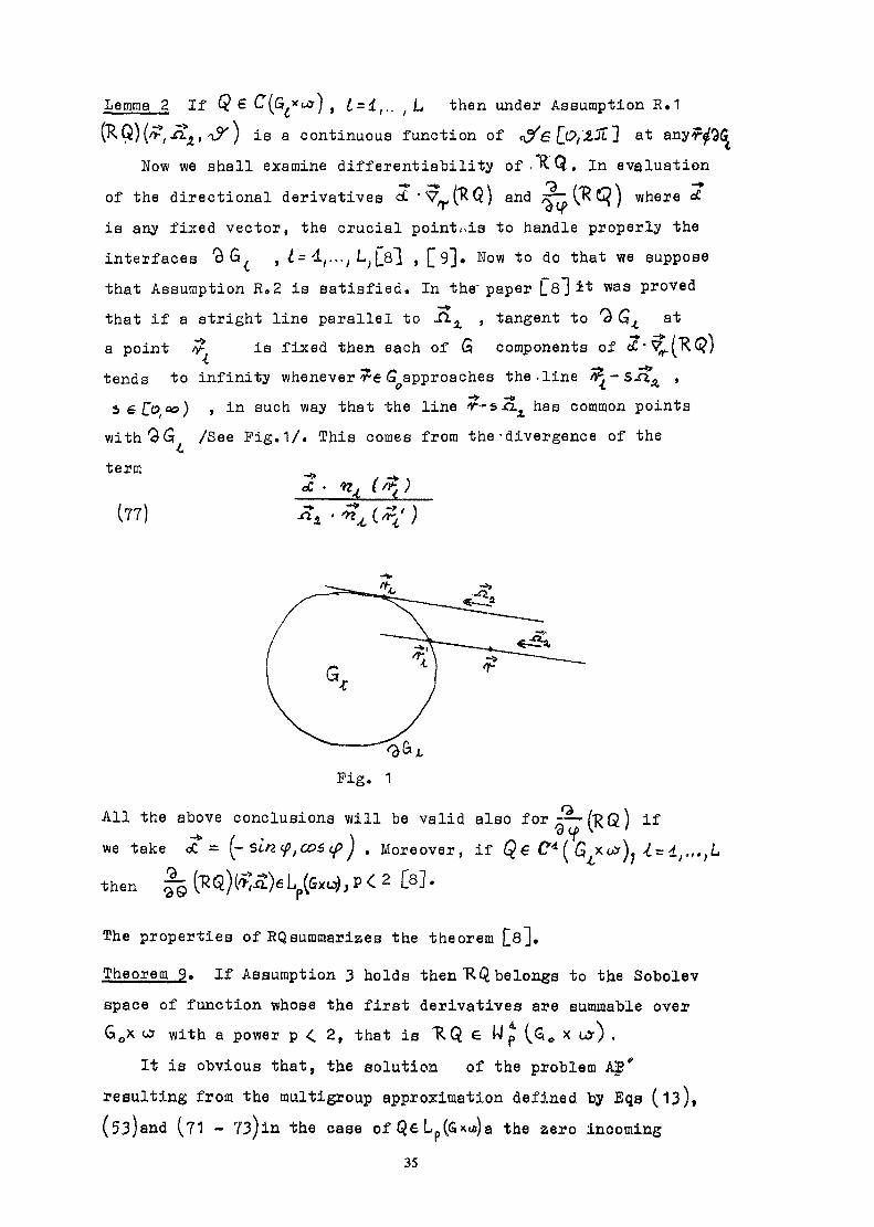
Now we shall examine differentiability of .XQ. In evgluationof the directional derivatives cC 'Vr(RQ) and Tv^C^^) where oCis any fixed vector, the crucial point.as to handle properly theinterfaces ß G . , t= 4,...; ,[ß\ , C^l« •Krow to ^° 'fc'aa't vve a^PP086that Assumption R.2 is satisfied. In the" paper [o] It was provedthat if a stright line parallel to -O. , tangent to 0 G^ ata point /r is fixed then each of G components of c£'tends to infinity whenever ve G approaches the.linese To, «») > in such way that the line T-sJl^ has common pointswith 9 G /See Pig.1/. This comes from the-divergence of theterm

2(77)

All the above conclusions will be valid also for z-^RQ) ifwe take ccT = (- St/2 tf, cos if> ) . Moreover, if QeC*(G xo*); ^^ d;.,.,then 2 [s].

The properties of RQ summarizes the theoremTheorem 9« If Assumption 3 holds then "RQ belongs to the Sobolevspace of function whose the first derivatives are summable overG0X u? with a power p < 2, that is KQ e Wp ($„ x

It is obvious that, the solution of the problem A5*"resulting from the multigroup approximation defined by Eqs (13),(53)and (.71 - 73)in the case of Qe Lp(<5xia)a the zero incoming

35

neutron flux that is f _ A j , - 0 is alao the solution to the equation

(J8) ^"RQ + R K t tThe properties of RQ are stated by Theorem 9« Now we shall

examine the operatorsfR«)with n V 1

Lemma 3 Suppose that

a) for each Z e S0 K (£,/«•) ê- L,^ ; [ -1 , 1] •

*) £C*) G L« CO 5then KRK is a bounded linear transformation from Lp(jS*to),into Ln (<a0 * o> ) , where°

- _«*PöC-l

Corollary 1 To any p, 1^P ^ °° it corresponds an integer ici (p)such that(KRK)u with -n n(p) is a bounded transforamtion from

into L^ (60* i*) . Tbe integer ti(p) is given by

Since KRK compact in any Lp (Go * w) » 1 4 P <°° then from

Corollary 1 it follows Lsl .Lemma 4 KRK is a compact transforamtion from i-pCG^w) into L<,(<3<,where p and q satisfy the conditions max (oC,p) t "* , max f d ,rf J^j ' ]Both Lemmas 2 and 3 imply the theorem ES],Theorem 10 The operators (K"R K) with n*} n(p) + l whereis given by Eq. (so) are compact transformations from Lpâ^Xinto L.OO C^„x^)-Combining Corollary 1 with Assumption R.1 we get £s3»Lemma_g For any u(6 L .# (Gox w) , under the Assumption R.Îthe function K^ 15 KQX^Ü) for a fixed A é W is an elementof Lip (,G0) where p, is any nol number such that

ifwhere 4. ^ <£ < 2» and -r •+ 4- =^ «*. et

36

The continuity of (K /R K Q)(£,.n.) with respect to Ais stated by the following lemma.Lemma 6 For Q € L xur) under Assumption R.f. (K KQ) (/r,for fixed reG. is an element of Lip ,( ) , where

i v tjb 4 et *Thus finally Lemmas 6 and 7 and Theorem 10 imply the theorem

%1>Theorem 11 Under Assumption R.1 all the operators'RK withn ^ *n (p) •+ 4- are compact linear transformations from i (G0Xinto a subset of L G ur) consisting of functions from Lip (Gfor any fixed -O- e Ly^ t belonging to Lip ..3/^^ for any e GOoand e[£,:rt-e] , and to Lip (C . 'O) for any /?f opand 9 ^ LOf^JiJ . The exponents ft and S' 'are defined inLemma 1 and 5 respectively.

Similarly from Theorem 9 and 10 it follows.Theorem 12 If Assumption R.2 is valid then^K) withis a compact operator from IL (G0X W') into

In the paper Ls it was proved that the spectral radiusof RE. is less then unity. Thus in it followsthat the solution of the neutron transport equationwith QeL p(G0xu?) is given by the formula

where oo

(31)/? e Lp.

If Assumption R.1 or R.2 are satisfied then the class ofcontinuity of >U is given by Theorem 11 or Theorem 12respectively.

Now we shall prove the behaviour of oC7?.'tt t^:/UL andQe'M.|V»here /m is the solution of the transport equation (?8).To do that we consider the equation obtained by applying theoperator OCV^ to the both aidas of Eq.(22):

37

(82)

where

(83) QtBy Theorem 9 , and belong to Lp(G0X<^) , p < 2 .Thus the decomposition (81 ) is valid for «C \7-> 'W- • The sameais true both for îo 'U and Tfo 'It . We have proved:Theorem 13 If we assume:

(i) Assumption R. 2 is satisfied(ii) « Q and 70 Q_ are bounded«

-( iii) 5 is diff erentiable with respect to f being theinterior point of each G^ } 1= d.,2,,- ••,** .

then the solution to the transport equation /Ü. belongs to~* — ** ^.1 More over for each derivative oC • \7 > IL t <fïf> /u

and -s /ti the decomposition ( 81 is valid.The results stated by Theorems (10 - 13) are not applicable

to the rectilinear problems» In the following vie shall studythe problem of smoothenss for two-dimensional rectilineargeometry.

Now we describe more precisely the geometry of the problemand introduce some definitions useful for further analysis.

We assume that the boundary 9 G0 of G0 is composed ofline segments • , =,...

3G= U 9 G.:. .We consider the convex set G to be a union of open sets (^ ,(.-4.,- L . For each 0 G i we have the following decomposition

where L- is the set of indices of all (Jojnains adjacentto GÎ, , K(sj) is the set of indices of all the linesegments Q Gr contained in the set Oßj oQ fîj andsubset of L 0 defined by the formula(86)

38

In the following the symbol n •• will stand for the normalvector to the line segment Q G-- . It is obvious that foaeach pair of (i/J ) and k 6 K(i,j) there exists ansuch that Kij =~nji . The set of all vertices of the polygonso G i , i = £?d,...;L Win be denoted by 41 .We introduce also

the sets;

(8?) MO :

and(88) ' *

All the line segments of ' o when extended give a finitecollection of lines in two-dimensional Euclidean space "R .

The intersection of all these lines with G = G» u 9 G»0 will bedenoted by f^ • Finally we denote by P^ the common part of Gand the lines joining any two points of U • The obviousrelations hold

(89) r° C r<. ° Consider a function f(/r] continuous in each G' t i-ir..,L .

Por any piecewise continuous •{•(/?) v/e introduce^., (/f*/ ti=ilZr..,Le L. , /f.4. . /< and ff) iSi..L to bej

limit values of •£(/?/ on 0 6ij? and 3 G i (7 in the following sense:',

if f € ^G^j then we take any sequence -[/^ ; /^ ê Gt. / /7?"4 /2 / . . • j*_converging to /v and put

(so) ft (?) =J

Similarly for /?-6-Oa i 0 we have

(91)• ri f - —•

The neutron transport equation ( 78 ) will be studied underthe set of assumptions which can be formulated as:

Assumption R.3(i) the conditions (.ii) and ( iii) of R.2 are satisfied,(ii) the geometry of the problem is described Eqs (82)-(84).To prove the properties of 'R Q we first examine the

39

behaviour of Çsgf-sfââ'JJi) the optical distancebetween a point T and the boundary 9 GO along -•&•£,

In turn to find the properties of O (/?", -Q. ) we mustconsider in details various cases of positioning of the line

, -Q.J defined by the equation?(92) rf

relative to the sets P0 and P. . Therefore in the followingwe introduce further definitions related to the geometry ofthe problem.

The set of all the points from P0 crossed by the line (92 )will be denoted by W^ ("" ; -£"*• a ) '•

(93) s Â& = ro nWith any element U € "sv*""/) we associate the set

(94)It is also useful for the further analysis to define the

set " n r l i j containing al l the vertices belonging to

(95) /fr- ) = n <*and the set w(| whose elements are all the unit vectorssatisfying the condition(96) ^ 3-t'ZÎj = ° > t = Y'"'(L ' JeLi '

where n.. is normal vector to*3Gn • Tke subset of url( whoseelements satisfy the condition (96) will be denoted by 07° .It is easy to see that to each .n eu w,, and^-eld itcorresponds a set M (^ J? ) of the integer triples (i,j<kj SUchthat (i,j<k)e ?('??,.a ) whenever(97) QGy c oC ("",-rt.J

Let us consider now a line c/71 given by equation«•Ï + 0=0,

where ^2 is the normal vector to c^7 and C is a constant«/ "* /-\ "\It is easy to find that the distance measured along c£(/ft •"•» /

between a point f" and the line c/79 is given by the formula

(98)

40

Thug vie have the following expression for the derivativeof d (#-, t <JF J with respect to £ along any unit vector ÔC(99)

How vue are in the position to formulate the lemmaLemma 8

Under Assumption R.3 the optical distance <j> ('r, -O-A ) hasthe following properties;(1^ QÂ^) is a continuous function for all -fta and f?(2) If /£ e /^ then D(/?(IIA) is a continuous function of T

for all Jtj 4 H'40«0 and for - «.€ H" ^1° ßuch that^4 (î-â.) is a finite collection of points.

(3) Por 7. 6 or - 6)-((ô the optical distance g(<?, -o.4) isdiscontinuous at any point *£ e H such that T Q ~ in the following sense: let us take two sequencesand {^nj convergent to the point -r , such that <fdfc.(p,3l}and 9*€(3T,27r) wbere^* _ -» ,/ .tj «(cus s/«/), U 4, a then

K • -3» ) - ™ Q (^ . 5i)Ä S $ 2 PHjiV*' a/ ^ . 5 v *j */ uikem~£ c kJ(4) Por AAeo>a and for any /r^ /^ we have the following

exression for the directional derivative:

where '-R S - 2 *^ 2 («) ,« ii^s^f) y"-"a -1

j§ (^r -f?A ) is a continuous function, 'U-- is a normalvector to the line segment ßßj; , /a (î-â,) an^ c^>(aee defined by Eq. (93) ,

(5) If assumptions of Point 4 are satisfied and moreover theset M (P, &.t) defined by Eq.(95) is -not empty thenat 'f the derivative oc-^ ( -cij) has a jump given bythe sum in ( 4 ) where the set s -0*) is replaced by

All the points of Lemma/, 8 / can be obtained aftercalculations based on the definition of g (.$ > -âJ and Eq

41

Let «T be one of the sequence defined in Point 3 ofLemma 8 . Let us consider another sequence •[ -H ] whereAê t<j such that the set M (/r*, -H^ ) is not empty and-£„, — »••<£» 6 «£" w,? » (î -0-*) O .For any function/(/r>, -aA) piecewise continuous in ^ and -£?* we can definedthe following iterative limits:

(100)and(101)

How we can formulate the following öorollary to Lemma 7which collects all the results concerning the behaviour ofQ(S£ jri ) > inherent to the rectilinear geometry:Corollary 2

(l) For any r 6 H and .aa e such that M( AX)4 0 theiterative limits. od ( ( xi A ) and Pa (/.fl) are different

in the sense of definitions (100) and ( 101 ) .(2) For any /r e T such that M (^, n"2) 9^ 0 the first

iterative limit in the sense of (101.) is infinite as resultof divergence of the terras

where 72 is the vector normal to the line segment towhich *r belongs.We conclude the investigations of the properties ofg (^f-^jt) by the lemma.

Lemma 9If g— Ç («T , -â ) exists then its behaviour is given

"" *by Lemma 8 and Corollary 2 where * is replaced by

Lemma 10Under Assumption R.3 the function 'U

considered as a function of i- and Afc for fixed «rehas the properties analogous to those or cC^r-^x) stated inLemma 8 and 9 and Corollary 2, DO].

42

Making use of Lemmas 8 ana 9 ana applying the techniqueof 8 vie prove the concluding theorem.

Theorem 14

Under Assumption R.3 the solution tt of the transportequation (46 ) with the boundary condition £ U = 0 has thexollowing properties!

(l) <?*V~^ exists for *r and 2z such that <£ («r,.fOn Qconsists- of .finite number of points. For A-VfU the expression

is valid if we replace "R Q by Q $ defined byfirst term of this expresion is the most singular one,(2) The conclusion ox the Point 1 is valid for A ni

we pu-c ot{3) I'he location of the discontinuities of -U is the same

as for *RQ given by Lemma 9«'i'he smoothaftss problem for rectilinear geometry was

extensively studied by kellog JJ9] ,Lemmas 8-10 recover part of Sallog's results. However

theorem 14 und the rest of results stated in £lo] give moredetail information about the singularities of the solution toth® transport equation»1. 1. 6. Conclusion

Prom the results of Sec. 5 it is be to concluded that thedesign of high order approximation algorithm solving boundaryvalue problem is an extrema.ly hard task. The. singularities of thesolution of this problem are not localized but they propagatealong stright lines, which contrary to the case of the diffusionequation, do not coincide with interfaces among regions ofdifferent material composition. Even in very regular case withno interfaces and constant cross sections the solution of the

4.transport equation belongs only to the Sobolev spaea W p p <2.Thus standard approximations used in theory of finite differenceor finite element methods solving the boundary value, problem

43

elliptic equation are of limited use when applied to thetransport equation. This problem was already noticed in earlypaper of Mika et al [20J concerning the influence of singularcharacteristic in £x algorithms in the two dimensionalNrectangular geometry.

It was proved by Stankiewicz 22] that due to the singularbehaviour of the solution, the local approximation for th«well known diamond scheme used in p codes for rectangulargeometry is only \\ , rt < 1 , where n is a mesh size.Two papers of Kulikowska \~9\ and 1*2 1\ for one dimensionalcylindrical and spherical geometries analyze the smoothnessproblem of the solution to the transport equation versus itsimplication for the convergence of > methods.

As for as the finite element approach is concerned in bothangle and space variables in two dimensions we may requireno interelement continuity of the flux but only the normalcomponent of the current. This may considerable increase thenumber of uknown coefficient to be determined. It seems thata version of hybrid method already applied in its simplifiedversion in DOIT J23lisa resonable approach to get local highaccuracy approximate methods and not to increase the memoryrequirement comparing to the standard finite difference methods.The DOIT scheme can be obtained in heuristic way as it wasdone originaly or more rigorously using GVP with test functionsdefined in a box as the exact solution of the adjoint transportequation with properly chosen set of boundary conditions onthe edges of the box 1 24] •

1.2«. IMPROVED SCATTERING MODELSThe neutron scattering kernel represents a key parameter

In the neutron transport equation, whose solution Is of fundamen-tal Importance for fission reactor design and operation.

The Influence of the number of terms In the N e l k t n modelon the d i f f e r e n t i a l and total scattering cross section is In-vestigated and an expression for the scattering kernel simpler

44

than Nelkîn's is developed. An approximate relation for deter m i -n i n a the cutoff energy for neutron upscattering is also proposed.£25J. Furthermore, the general molecular o r i e n t a t i o n a v e r a q i n qw i t h respect to orientations of the i n c i d e n t and slow scatterinqneutron ha» been a p p l i e d . As a result it was shown that Krieger-N e l k i n approximate orientation averaging can be successfully ap-p l i e d to the most general form of molecular anisotroplc v i b r a -tions J26].

Improved expressions for microscopic kernels of thermal neut-ron scattering on water molecules are deri v e d . The improvementsconsist in a more r e a l i s t i c d e s c r i p t i o n of dynamic properties ofwater molecules and in an exact treatment of c o l l i s i o n time w i t hall rota t iona1-vI bra t iona1 phonons taken into account.

Concerning the dynamic properties, the m a i n improvement isrelated to the i n t r a m o l e c u l a r v i b r a t i o n s . They are represented bya two d i m e n s i o n a l anisotropic o s c i l l a t o r l y i n q in the plane of thewater molecule. One a m p l i t u d e vector is oriented in the OH - bondd i r e c t i o n , the other bei n g p e r p e n d i c u l a r to it. The trans' ft i ona 1motion is represented by a m o d i f i e d free gas model and the rotatio-nal motion by a quasitor s Ional Isotropie o s c i l l a t o r p e r p e n d i c u l a r

to the plane of the molecule.Instead of the short and long time c o l l i s i o n approximations,

an exact c a l c u l a t i o n of c o l l i s i o n time ts i m p l i e d . This enabledthé extensive studies of the influence of the different forms ofmotion of molecules on thermal neutron scattering.

Taking Into account the exact c o l l i s i o n time, some charac-t e r i s t i c effects were observed, as: (1) quantum effects of e x i s t i n qthe intramolecular vibrations, as well as combined effects of scat-tering on the v i b r a t l o n a l and rotational - v l b r a t l o n a l phonons, (2)a h i g h l y pronounced qua sieI 1 as t ic peak and the multiphonon scatte-ring on the rotational phonons.These effects were p a r t i c u l a r l y pro-nounced at the foreward scattering of thermal neutrons«

45

1.3. ENERGY DEPENDENT ANISOTROPY OFELASTIC SCATTERING AND NEUTRON SLOWING DOWN

1»3»1« Introduction

The anisotropy of elastic scattering of neutronsis negligible at energies below - 2 MeV, but it is verypronounced at higher energies. Consequently, in fast-reactorcalculations, the anisotropic scattering can play a substan-tial role in the magnitude and shape of the spectrum. Apartfrom the numerical treatment and numerous computer codes,2 r ~Te.g., NC '[28J , which can always lead to the desired solu-tion of the problem, this contribution considers an analy-tical procedure for solving the problem of neutron slowingdown in an infinite medium with an energy-dependent aniso-tropy of elastic scattering.

The present approach to the analytic treatmentof the energy-dependent anisotropy of elastic neutron scatter-ing can be outlined as follows: The scattering functionP(u', Au).is .defined and expanded in terms of Legendre polu-nomials ß9J and the energy-dependent coefficients ofthe expansion are determined from experiments [30 » ^nthis expansion of P(u', Au), it is possible to carry outmatrix degeneration of the kernel of the slowing-down equa-tion, and the matrix separable kernel allows the integralequation to be transformed into a differential equation interms of Green's slowing-down functions.

The order of the obtained differential equationdepends on the order of expansion of the scattering functionvia Legendre polynomials. In some cases it is possible toobtain analytically Green's slowing-down function. In gene-ral, this function is determined by standard numerical methodsfor solving sets of differential equations.

The idea of solving the integral slowing-downequation by degener-ation of the kernel is not new [31 _ 33]Note applies this idea to a suitably transformed scatteringfunction to obtain separable kernels. The general case ofP approximation is considered. The present approach allowsgaining deeper insight into the associated phenomena.

1.3..2* Integral slowing-dotm equation

The transport equation for the slowing down ofneutrons (Ref.2) 1n an infinite monoatomic medium containinga uniformly distributed source is

46

fuMu)»(u)-S(u)+ ï1(u')»(u')P(u'* u)du''u-e

It representsa simple balance) equation for the neutrons Ina unit lethargy Interval surrounding u. The left side of thisequation is the collision density and stands for the numberof neutrons lost per cm /sec due to absorption and scattering,while the right side is the number of neutrons gained eitherfrom the source or by in-scattering from other energies. Wedenote by P(u'- u) the scattering function and by P(u'-» u)du'the probability of a neutron surviving a collision at a lethargyu'and arriving at a lethargy interval u,u+du.

1»3«3» Differential cross section

In particle transport theory it is customary torepresent angular distributions by series expansion viaLegendre polynomials [29~3 • This form is very suitablefor studying the energy dependence of anisotropy of elasticscattering; in this representation the coefficients of theseries expansion are energy dependent.

The angular dependence of the cross section ofneutron scattering is

(!)

where BÊ) are the experimentally determined energy functions(Ref.3) and other symbols have their standard meanings.

Relation (1) san be rewritten in the form of a powerseries of u. In this case, crÊ, u) is identically represen-ted by a polynomial in terms of \i instead of by Legendre poly-nomials. This form is not usual in the literature; however,it is very convenient for the present purposes:

°s(E,y) - l a.(E)pn. (2)

1«3«4« Scattering functionThe scattering function, i.e., the probability that

a neutron of lethargy u'arrives, after a collision, in theunit interve.l around lethargy u is usually denoted by P(u'-«- u)29 -and 32 • If the anisotropy of scattering is energy

independent, this function is completely determined by the

47

difference .of lethargies after and before the collision,u - u'<= Au, irrespective of u" ; i.e., it can be identicallyrepresented as a function of Au:

P(u'+ u) = P(Au). (3)

If the anisotropy is energy dependent, this does not apply.Although the definition of P(u'-»- u) covers both cases, itis necessary to redefine the scattering function to avoidconfusion. The scattering function for an energy-dependentelastic scattering is P(u', u '-» u), i.e., P(u'. Au); thus,

P(u.' u'-* u) £ P(u'. Au). (4)

In general, Eq.(4) requires specifying a reference energyEQ. giving zero lethargy, whereas Eq. T3 does not.

The scattering function in energy space followsdirectly from <rs(E, u); i.e.,

<rs(E,v) .Ps(E'w) =

with

b.(E) = crs(E)

By d e f i n i t i o n ,

P ( u ' , A u ) d u = - P ( E , u ) d p .

w i t h the i n t e r r e l a t i on of v a r i a b l e s•*.-and

2A A2+l————-u + ———,= exp(u'- u), (6)

where A represents the atomic weight of the scatterer

48

1.3»5. Matrix form of the scattering function in theP_ approximation*"" H ' — "

The scattering function is, by its nature, a proba-bility distribution. For an energy-independent anisotropy ofscattering, this probability distribution depends only on twosuccessive neutron states having different lethargies. If theanisotropy of scattering is energy dependent, the scatteringfunction is simultaneously dependent on both the energy of theincident neutron and the energy difference caused by the col-lision. This property of the scattering function makes theintegral slowing-down equation unsolvable except by numericalmethods. However, the expansion by Legendre polynomials offersa possibility of expressing P(u', Au) in a matrix form. Inthis representation, P(u', Au) is exnressed as a product ofthree matrices where the first matrix is a constant rowmatrix, the second 1s a square matrix dependent only upon u',and the third is a column matrix dependent only upon u [341« ,In general, forms "(1), n(C), and n(g) of these matricescorresponding to the Pn approximation, can be obtained byinduction. Consequently, 1n the P approximation,

nP(u', Au) « n(1)n(C)n(g). (7)

Matrix n(1) is a 1 x (n + 1) matrix, where n denotes theorder of approximation employed for expanding o' (E,u) byLegendre polynomials, Eq. (1); all coefficiens of n(l) areequal to unity. The n(g) is a (n+l)xl column matrix havingterms of the form exp(-iu), i=l ,2 ,.... ,(n + l). Matrix n(C) isa square lower-squew matrix with all terms dependent on theneutron energy (I.e., lethargy) before collision.

1.3*6« Gareen^s slowing-down function

The integral equation of the Green's slowing-downfunction is (Refs. 2 and 5)

G(u)= JG(u')P(u',Au)du'+ 2<S(u). (8)

Using the P expansion of differential scatteringcross sections, this equation can be transformed to a lineardifferential equation of order n+1. This is performed bymatrix degeneration of the kernel of Eq. (8) and consecutivemultiplying by en and differentiating n+1 times. The obtained

49

equation has the following form:

Dn+1[G(u)eu]=Dn{G(u)IC(u)[9(u)eujeu}

I Dn.k((G(u)IC(u)|ok[g(u)eu]}eU)euj

+ Dn+1(s(u)eu], (9)

whereD.n(a(u)l- ^Hut---^««11))---«11)«")1 ' 1 2 n n 2 ]

andI = "(D

C(u). "(C)g{u)= n(g).To obtain the solution for Green's slowing-down

function, (n+1) initial conditions are necessary. These canbe obtained from Eq.(8) and its first n derivatives foru •* 0. In the case of nonabsorhing media |aa(0) ]= 0, theybecome

G, .. = lim P(0->u) = lim P(0,Au)' '

,.»G i = U(o ) u odu i=l du

k=l,2,...,n. (10)

1.3»7. Results and discussion

On the diagrams given in this Note, Green's functionsand slowing-down densities obtained for various cases ofscattering cross-section approximations are denoted by P , f, ,and Pp. However, it is useful for physical discussion of theresults obtaired to mention here that these approximations are

50

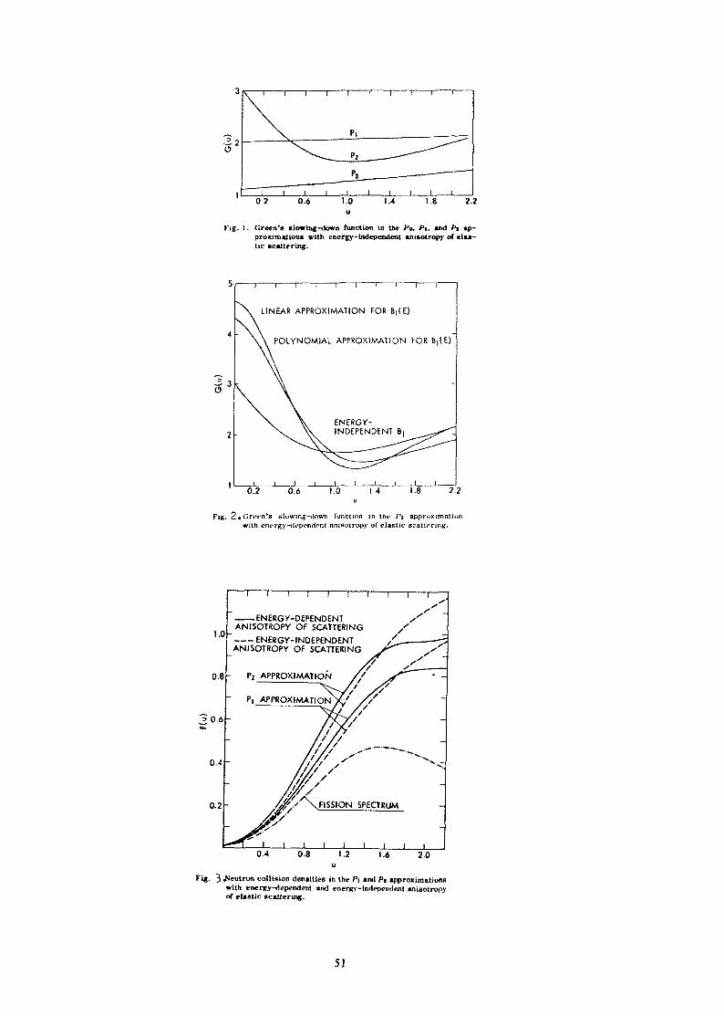
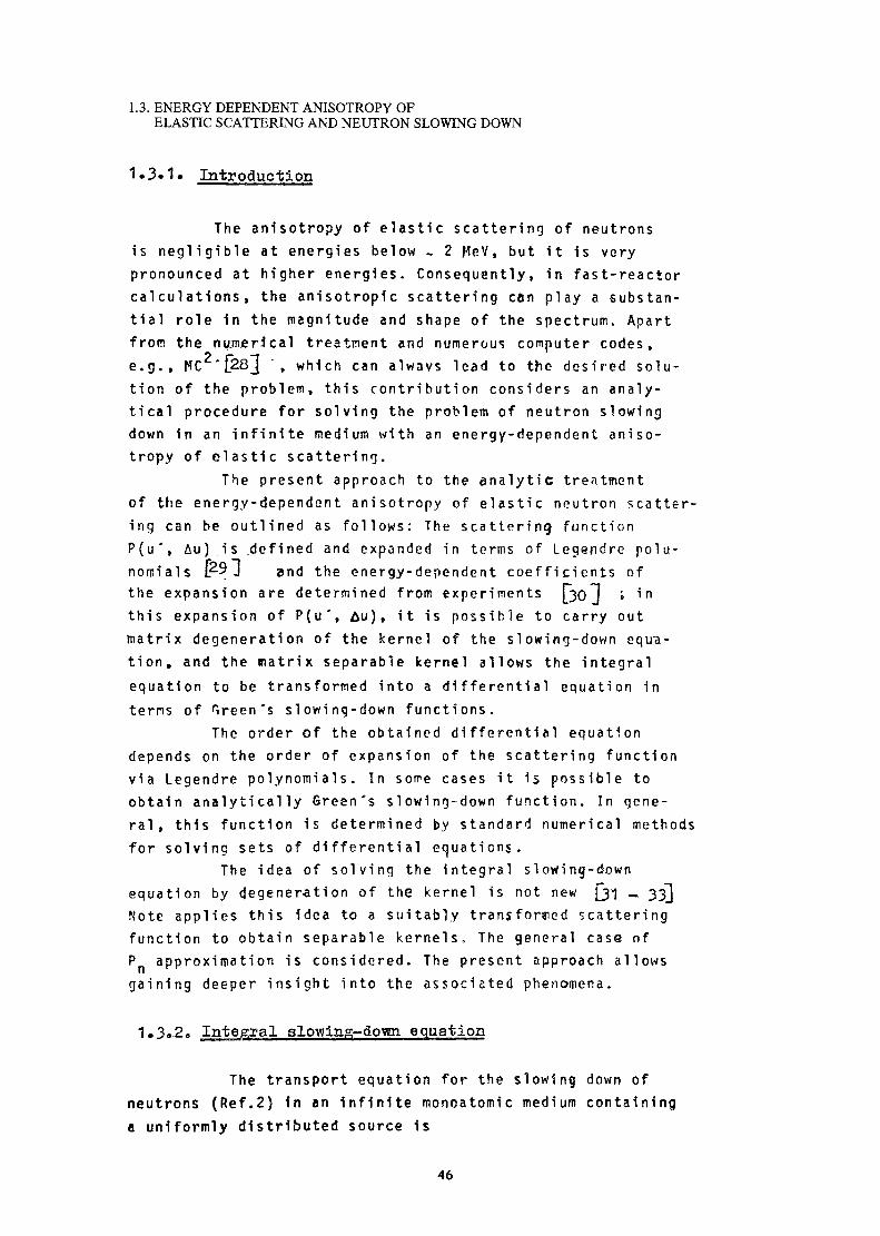
Fig. 1. Green'» slowing-down function in the Pa. Pi. and PI ap-proximations with energy-independent amsotropy of elaa-tic scattering.

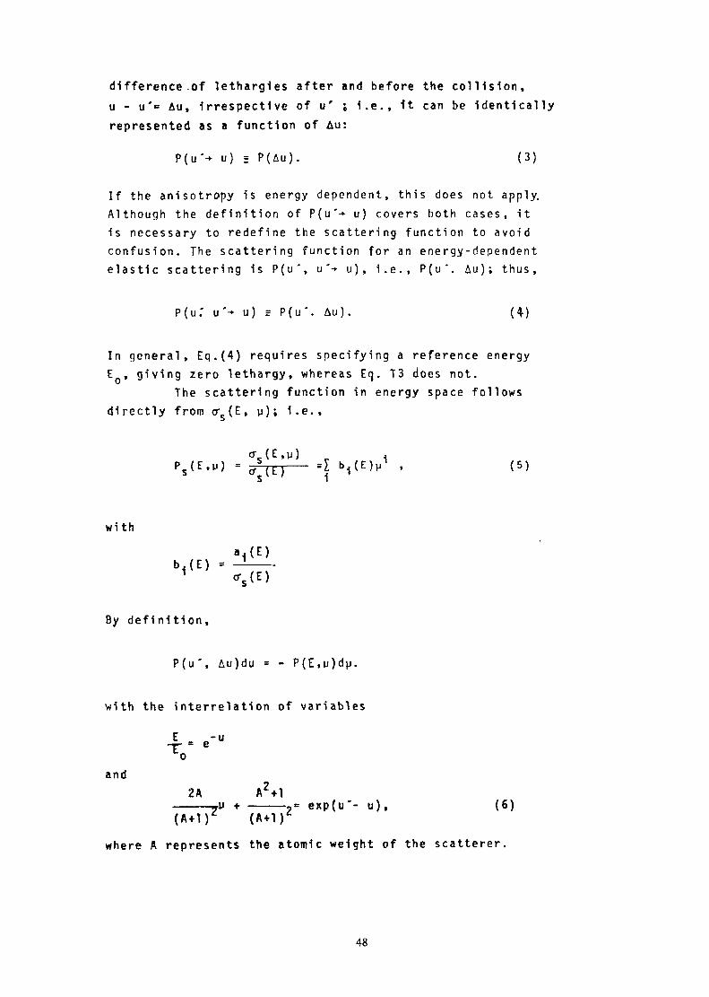
LINEAR APPROXIMATION FOR B|(E)

POLYNOMIAL APPROXIMATION FOR Bi(E)

Fig. 2»(.îr«H'n's slowing-down funct ion in the Pz approximationwith cniTgy-dopendent amsotropy of elastic scattering.

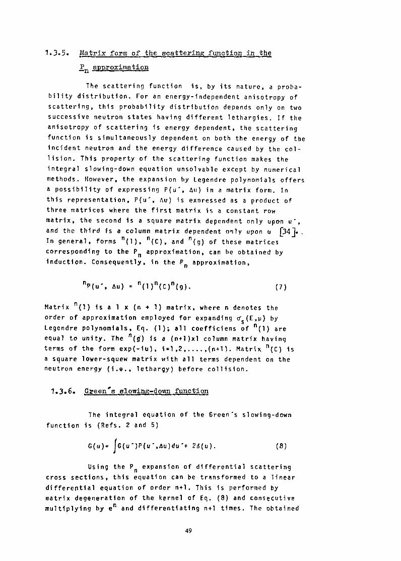
ENERGY-DEPENDENTANISOTROPY OF SCATTERING—— ENERGY-INDEPENDENTANISOTROPY OF SCAHERING

PJ APPROXIMATION

PI APPROXIMATION

I———I——I——I——I I i l i2.0

Fig. 3 Neutron collision dentitles in the Pi and P, approximation«with energy-dependent and energy-independent anisotrop)of elastic scattering.

51

equivalent to the isotoplc scattering, linear dependence,and the parabolic dependence of the scattering cross sectionon the cosine of the scattering angle in the center mass system,respecti vely.

Figure 1, which illustrates the cases of energy-independent anisotropy, indicates the importance of takinginto account the anisotropy of elastic scattering in solvingthe problems of neutron slowing down. Approximation P, favoursthe scattering at small angles so that the Green's slowing-downfunction values in the whole observed lethargy interval areconsiderably higher than those obtained for isotropic scatte-ring. With respect to the results obtained experimentally, theP~ approximation represents quite satisfactorily the dependenceof the cross section on the scattering angle. The experiments(Ref.4) show that in the examined case of deuterium the proba-bility of scattering of neutrons of the energy of several HeVis the greatest for small scattering angles and the angles near180 deg, i.e. scattering probability is the greatest for verysmall and very high energy losses. This characteristic isevident in Fig.l, where Rreen's slowing-down function is thehighest near u=0 (E«=10 MeV) and u = 2.2. At the same time, thesetwo lethargy values limit the interval of maximum neutronlethargy Increment in the collision with deuterium atoms.

Figure 2 presents Green's slowing-down function inthe P~ approximation. A great difference was observed betweenenergy-dependent and energy-independent anisotropy. This dif-ference is to the greatest extent affected by the initialconditions used in solving the slowing-down differential equa-tion. The initial conditions are expressed by the coefficientsof B, , which means that they are energy dependent as is B,itself. Green's functions for energy-dependent and energy-independent anisotropy w i l l depend on the energy of the source[for Green's function calculations: source = 2o(u) , sincethe initial conditions in the first case change with changingenergy, while in the second case they are constant.

Comparison of the results obtained by P, and P_approximations for Green's slowing-down functions leads us tothe conclusion that in such calculations it is necessary touse at least a P- approximation by which the dependence ofthe scattering cross section on the scattering angle is muchbetter presented.

Figure 3 shows that the P- approximation gives highercollision density (by approximately 25£) in the vicinity of1 MeV compared to that obtained by the P, approximation, bothfor the energy-dependent and energy-independent anisotropy.

52

This difference arrives since the P-, approximation underesti-mates neutron scattering under y = l and considerably overesti-mates this scattering under ii = 0.

Furthermore, Fig.3 allows the evaluation of the in-fluence of the energy-dependent anisotropy of neutron scatte-ring on collision density. The 10% higher collision densityabove 2 MeV and 20# lower collision density in the vicinityod 1 MeV obtained with the energy-dependent anisotropy qualifythe improvement introduced by this energy dependence. Obviously,the introduction of energy dependence in any serious calculati-ons of neutron collision density at high energies is welljustified.

The dependence of the coefficients of B, on energycan be satisfactorily presented by the third- and fourth-orderpolynomials employed in the paper.

Keierences

1* M.Borysiewiez, ji.otankiemiez, Weak Solution and ApproximateMethods, Jour.Math.Anal.Appl., b8. 191 (1979)«

2. M.Borysiewicz, R.Stankiewicz, Variational Formulation andPromotional Methods for the Second urder transportEquation, Jour.Math.Anal.Appl., 21» 210 ,(1979.).

3. I'.Mazuradar, Generalized Prelection Theorem and weakBoneoercive involution Problem in Hubert Space, Jo or »Math.AnaLAppl., 40, 143 (»974J.

4. M.Borysiewicz, G.Spiga, Approximate Methods SolivingVariational Problems Generated by Noncoercive Forms.Progress Keport, IAÜA Contract 1236/RB {1978}.

5. J.M.Thomas, Sur l'Analyse Numérique des Methods d'ElémentsFinis Hybrides et Mixtes Thèse Université Pierre et MarieCurie, Paris (1977).

6. J.P.Aubin, Approximation des Espaces de Distributions etdas Operateurs Différentiels, Bull. Soc. Math. France,Mémoire 12 (1967).

53

7* M.Borysiewicz, Approximation Theory and Homogenizationfor tbe Neutron Transport Aquation» Proc. Joint laJïTech* Com. Meeting, Homogenization Methods in ReactorPhysics, Lugano {1978.}.

8« M.Borysiewicz, G.Spiga, smoothness of th« Solution to 2-DHeutron Transport equation, Atti dell'Académie délieùcienze di Modena, 25 (1979)»

9. i'.Kulikowska, Singularities of the Solution to the Ueutrontransport .aquation in Cylindrical u'ymm«try, ïïukleonikaVol 21, Ho ;j, 589 (1976).

10. M.Borysienicz, K.Kruszynska, ùtBoothaMs of the Solutionof the 2-D Neutron Transport equation in the Polygon Region,A-Gomfcernenergie, 34. 11 (1979).

11. I.Babuska, solution of Interface Problems by Homogenization,SIAM Jour. Math. Anal. J, 603 {1976,).

12. V.S.Vladimirov, Mathematical Jrroblems in the One-VelocityTheory of Particle Transport, Tr.mat.Akad.Uauk SS&'R, (£, 1(1961j.

13. S.Kaplan, J.A.Davis, Canonical and Involutory transformationsof the Variational Problems of Transport Theory, Hucl.Sei.2ng*. 28» 166 (1967).

14. J.A.Davis, Transport isrror Bounds via P^ - Approximations,,Hucl. bei. Jung., 31, 127 (1968,).

15« A.J.Buslik, Bxtremum Variational Principles lor theMonoenergetic Ueutron Iransport equation with ArbitraryAdjoint Source, Hucl.Sci. ng., 3>. 303 (1969).

16. 3.S.Kaper, a.K.Leaf, A,J.Lindeman, Formulation of a nitz-Galerkin ïype Procédure for the Approximate solution of theHeutron Transport Equation, J.Mata.Anal. Appl., 50. 42 ,{1975 ).

17. P.ailvennoinen, A.Selfadjoint Porm of the Mnear transportEquation, J.Math.Anal.Appl., J , !?2y (1973)»

54

18. J.Pitkaranta, On the Variational Approximation of theIransport operator, J.jaath.Anai.Appi., 54« 419 (1976),

19. K.ïs.jxellog, Pirat Derivatives oi Solutions of the Planeïleutron transport equation, xech.iüoüe ua-YSj, Institutefor Fluid Dynamics and Appliea Mathematics University ofMaryland (1974J.

20. J.Arkuszewski, T.Kulikows*.a, J*Mika, Eifecte of Singularitieson Approximations in S me thuds, JSiuua..Sci..Qng., 49. 20,(1*72).

21. i'.iuilikowska, .einige Difference Approximation to the TransportEquation in Spherical Symmetry, Nukleonika J^ Bo 6, 521 (1974).

22. R.Stankiewicz, Smoothness of the Solution to the ïirae -Dependent 1'ransport Equation in Connection with tue finiteDifference Approximation. Progress Keport lA A ContractKo 123b/KB (1973).

2j. C.Maeder, Modified Versions oi the u.'wo - DimensionalTransport I'faeory Method D01$, EIR Bericht No 240 (1973).

24« J.Arkuszenski, M.Borysiewicz, New Derivation of DOlT bcheme,unpublished results (1977)»

2b. M.l.Markovic, Some remarks on the Ueliin model for neutronscattering in water, Nuclear Instruments and Methods, 1061973 , b19-524.

2b. M.I.Markovic, Justification of ürieger-Nelkin averagingin anisotropic molecular vibrations, J. Fftys. B: Atom.Molec Phys., Vol. 7, No 9 1974, L30i>-L309.

27. J.Pop-Jordanov et al., Some improved methods in neutrontransport theory, IAEA Meeting on Methods in Neutron TransportTheory, Warsaw, 4-7 December, 1973.

228. B.J.Toppel et al.,"MC - A Code to Calculate MultigroupCross Sections", ANL-7318, Argonne National Laboratory 1967.

55

2y. A.M.Weinberg and E. .Wigner, fhe Physical Theory of NeutronChain Reactors, The university of Chicago Press, Chicago,Illinois (1958).

30» M.U.lsrikolaev and IT.O.Bazazjanc, "Anizotropija uprugovorasejanija neitronov", Atomiz«a, Moskva (1972.).

31. M.Cadilhac and M.Puöol, J. Hucl. energy, 21, 58 (ly6?).32. .u.Stefanovic, Huol. t>oi. Eng., £1, 394 (1970 ).33. M.Becker and a.jsurns, Hucl. Sei. ûng., j|2., 10 (1970).34. w.Stefanovic, Hucl. Sei. Jsng., 59. 194 (1976).

56

Chapter II

ADVANCES IN ITERATIVE METHODS

B. BEAUWENS, J. ARKUSZEWSKI, M. BORYSZEWICZ

1 . INTRODUCTIONThis chapter summarizes the results obtained in the field of linear iterative me-

thods, within the activities of the Coordinated Research Program on Transport Theoryand Advanced Reactor Calculations,at the Kurchatov Institute (LEBEDEV et al.)» at theInstitute of Nuclear Research of Swierk (WOZNICKI et al.) and at Brussels University(BEAUWENS et al.), or developed in cooperation between these groups.

2 . CONVERGENCE THEORY

The general convergence theory of linear iterative methods is essentially based onthe properties of nonnegative operators on ordered normed spaces . The following as-pects of this theory have been improved : new comparison theorems for regular split-tings, generalization of the notions of M- and H-matrices, new interpretations ofclassical convergence theorems for positive definite operators .

2.1. Notations

We consider here the solution of a linear systemA x = b , xSV , b € V , AG je(V) (2.1)

where V denotes a real or complex n-dimensional normed space and £ (V) the normed al-gebra of endomorphisms of V, by iterative schemes of the first order, i.e. of theform

where (x ), m=0,1,2... is the sequence of successive iterates, B e £ (V) is assumednonsingular and A = B-C is the splitting which defines the method. The associatediteration operator is T = B~ C with spectral radius r(T).

We assume that the normed space V is the direct sumk

V = @ V. (2.3)i=1 1

kof k subspaces V. of dimensions n. with £ n. = n. Thus any vector x e V has a1 k x i=1 *unique decomposition x = Z X. into "block-components" X- = P.x where P. is thei = 1 1 1 1 1corresponding projection operator of V onto V. and any operator A s £ (V) has aunique decomposition into "blocks" A. . = P. A P., with

k(Ax),= Z A.. X- (2.4)

57

The decomposition (2.3) will be denoted by ir. An operator A e <C(V) will be termedlower (resp. strictly lower, upper, strictly upper) triangular with respect to IT ifA. . = 0 for i < j (resp. i $ j, i > j, i 5 j) and diagonal if A. - =0 for i ^ j . Ifti^= 1 for all i e [ 1 ,k] , we say that IT is a point decomposition-'of V.

We shall make use of the following operation

( a S A ) . = c A (2.5)

called ^-multiplication (with respect torç) of the operator A e JC(V) by the kxk matrixthe Hadamard multiplicationnotations

ex = ( 0 = - ) ; when TT is a point decomposition, it reduces to tof matrices [44] . In addition, we introduce'the following

diag(A) = I * A , offdiagfA) = A - diag(A) (2.6)

where I is the kxk unit matrix.

For practical implementation, it is worthwhile to observe here that the scheme(2.2) and the residual scheme

-1X , .4 — X — Jj I/\2C — D J I £ • / Inn" l m m

though, mathematically equivalent may be of markedly different computational comple-xity t 18 ] .

2.2. Regular splitting theoryIn this section, we further assume that V is a real ordered norm|d space with non-

negative cone C (proper, closed, convex and with nonempty interior c) and we use thefollowing terminology : x e V is called nonnegative (resp. positive) and denotedx >, 0 (resp. x > 0) if x e C (resp. x e Q ; an endomorphlsm A of V is called nonnega-tive (resp. positive) and denoted A >, 0 (resp. A > 0) if x >, 0 =*Ax 5 0 (resp. x >, 0,x 7* 0 =»Ax > 0) ; it is called semipositive if x * 0, Ax / 0_î»Ax > 0; it is calledmonotone if Ax 5 0 =*x 0, i.e. if A is nonsingular with A 5 0.

With these notations, the classical convergence and comparison theorems may besummarized as follows.Theorem 2.1 (convergence theorem)

Let A, B, C e jC(V), A = B-C be such that B is nonsingular and T = B C nonnegative;then the following conditions are equivalent(1) r(T) < 1;(2) I-T is monotone; 1(3) A is nonsingular and G = A~ C 5 0 ; ,(4) A is nonsingular and r(T) = r(G)/(1+r(G)) where G = AC;[$] there exists x > 0 such that Tx < x.

Theorem 2.2 (comparison theorem)

Let A, B-, C, e JO(V) , A = B. - C-, i=1,2 be such that B. are nonsingular and ,T. = B^; C- nonfiegative and convergent. Then G., $ G2=* rCr.) £ r(T2) where G. = A~ C- .In particular, if B^ are monotone and C. nonnegative, C* <: C2=* r(T..) * r(T2) .

Theorem 2.5 (strict comparison theorem)

Let A, B- C- e ,C(V), A = B. - C-, i=1 ,2 be such that A is monotone with A > 0, B-are nonsingular'and T- = B7l 0. are nonnegative. Then 0< C, $ C,, C, ^ C9="r(T1) <r(T2). 111 l z l z i

These comparison theorems can be applied only when the operators C- and C2 orG-, and G2 are comparable, a condition that makes them unsuitable for many compari-sons between factorization iterative methods.

58

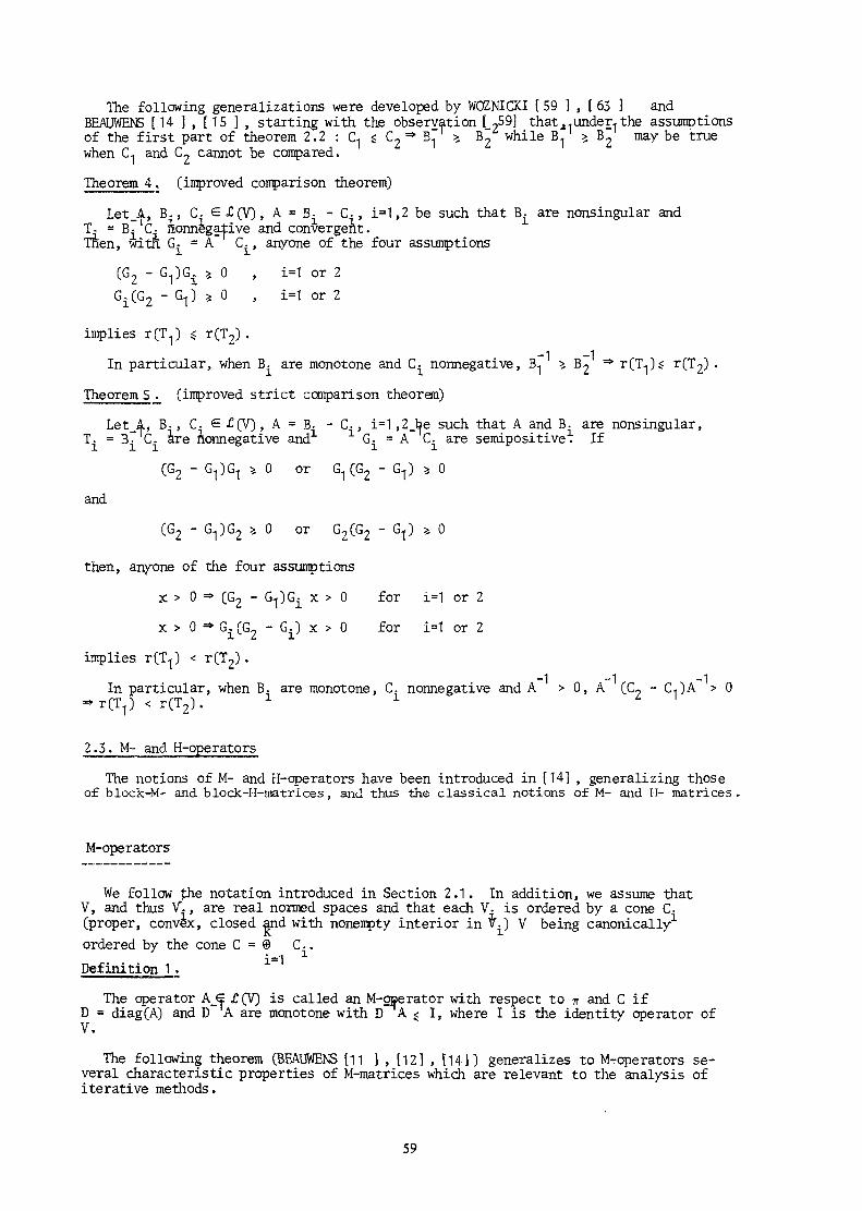
The following generalizations were developed by WOZNICKI [ 59 ] , [ 63 ] andBEAUWENS [ 14 ] , [ 15 ] , starting with the observation [ 259] that „under. the assumptionsof the first part of theorem 2.2 : Cj s C2 =* B j" >. B2 while B^ >f B~ may be truewhen G* and C7 cannot be compared.Theorem 4 . (improved comparison theorem)

Let_A, B. , C- e £(V) , A = Bi - C- , i=1 ,2 be such that Bi are nonsingular and!i = Bï Ci Aonnegative and convergent.men, witn. G- = A~ C. , anyone of the four assumptions

(G2 - G^G. * 0 , i=1 or 2Gi(G2 - G.J) ;> 0 , i=1 or 2

implies rCT^ 5 r(T2) .

In particular, when B- are monotone and C^ nonnegative, B^ >, B2 =* r(T-|)s

Theorem 5. (improved strict comparison theorem)

Let_A, B, , C- e £(V), A = B. - C. , i=1 ,2_ê such that A and B. are nonsingular,T- = B~ C- are nonnegative and G- = A C. are semipositive. If

(G2 - G1)G1 * 0 or G^(G2 - G.J) * 0

and

(G2 - G^G2 >, 0 or G2(G2 - G^ > 0

then, anyone of the four assumptions

x > 0 =* (G2 - G-()Gj_ x > 0 for i=1 or 2

x > 0 => Gi(G2 - G^ x > 0 for i=l or 2implies r(T ) < r(T2) .

~1 -1 -1In particular, when B. are monotone, C. nonnegative and A > 0, A (C7 - C,)A > 0< r(T2). x x

2.5. M- and H-operators

The notions of M- and H-operators have been introduced in [14] , generalizing thoseof block-M- and b lock -H-ma tri ces , and thus the classical notions of M- and H- matrices.

M-operators

We follow the notation introduced in Section 2.1. In addition, we assume thatV, and thus V., are real normed spaces and that each V. is ordered by a cone C.(proper, convex, closed and with nonempty interior in V.) V being canonically1ordered by the cone C = @ C..

* —"1 ^-Definition 1 .

The operator AC jC(V) is called an M-operator with respect to w and C i:D = diag(A) and D~ A are monotone with D A g i , where I is the identity q

ifoperator of

V.

The following theorem (BEAUWENS [11 1 , [12] , [Hi) generalizes to MTOperators se-veral characteristic properties of M-matrices which are relevant to the analysis ofiterative methods.

59

Theorem .6Let_A, R G £ (V) be such that R is diagonal and monotone (with respect to TT and C)

with R A s I ! then the following conditions are equivalent :(1) A is an M-operator;(2) A is monotone;(3) there exists x => 0 such that Ax > 0;(4) there exists x > 0 such that Ax > 0 ; ^(5) there exists x > 0 such that Ax >, 0 with f_1 A. . X- > 0 for all i € [ 1 ,k] ;(6) there exists x > 0 J k

J •>such that Ax >, 0 with j R~| A^X. > 0 for all i 1 ,k] ;

(7) IT R"1A is convergent; J=1 J :(8) R A is monotone ; _1(9) A is nonsingular and A, R >, Ij

(10) A is nonsingular and A % R~ ;(11) .there_exists a convergent splitting A = B-C of A such that B is monotone and

T = B C is nonnegative; _1(12) any splitting A = B-C of A, such that B is monotone and T = B C is nonnegative,

is convergent; _•,(13) D = diag(A) is monotone and J = I-D A is convergent;(14) for any kxk matrix a = (<*;.:) of scalar parameters such that 0 g a^ $ a^ for

i 7e j with 0 < a - - , the operator A = a* A is an M-operator; J

(15) there exists lower and upper triangular M-operators, L and U respectively, suchthat A = L P U with P = diag(L) = diag(U).

H-operators

Again, we follow the notation of Section 2.1, the spaces V and V- being now realor complex. In addition, we assume that a vector norm (t) p. is given on eachsubspaces V-, with values in some ordered real normed space V - , i e [ 1 ,k] .

Thenk

p(x) =1 p.(P.x) (2.8)i=1

is a vector norm on V, with values inV o = ® V C2.9)

kcanonically ordered by C = @ C .. A vector norm p(x) on V, constructed in thiso i=1 01way will be called compatible or associated with the decomposition ir of V. The cor-responding decomposition (2.9) of V will be denoted by ir ; the notations diag(A)and offdiag(A) will be understood with respect to ir for the endomorphisms of V andto TT for the endomorphisms of V .Definition 2.

Let p(x) be a vector norm on V, with values in V , compatible with the decomposi-tion IT of V. Then A e jC(V) is called an H-operator with respect to p if D = diag(A)

(t) A vector norm p(x) on V is an application from V to some real ordered vectorspace V such that : (1) p(Xx) = |x|p(x); (2) p(x+y) « p(x) + p(y) ; (3) x f 0-pCx) P 0.

60

is nonsineular and if J = I - D 'A has, with respect to p, a convergent nonnegative upper bound '^ A e jC(V) is called an H-operator with respect to ir if there exists avector norm compatible with ir, such that A is an H-operator with resnect to p.

The following result (BEAUWENS [14 ] ) generalizes to H-operators, propertiesobtained by ROBERT[50][51 ]for block-H-matrices ; by an M- lower-bound, we understand alower bound which is an M-operator with respect to ir and C in V .

Theorem 7 .

Let p(x) be a vector norm on V, compatible with the decomposition IT and letA 6 £(V) . Then, with respect to p, the following conditions are equivalent

(1) A is an H-operator; _..(2) D = diag(A) is nonsingular and D A has an M-lower bound;(3) there exists a nonsingular diagonal operator S S JC(V) such that SA has an M-lower

bound.

2.4. Positive definite operators

It is generally considered that convergence theorems for linear operators fall intwo categories being based either on positive definiteness assumptions with respectto some scalar product or on nonnegativity assumptions with respect to some orderednormed space structure. In [ 20 ] I , it was shown that all known results of the firstkind can also be viewed as consequences .of the general relations between monotonicityand convergence in ordered normed spaces .

This interpretation can be developed in the general context of complex unitalBanach algebras and B algebras; in this way it actually leads to generalizations ofthe results previously established by Hubert spaces techniques.

However, to give a quick insight into the techniques used, we only report a parti-cular example, in the framework of a finite dimensional Hubert space, referring to[ 20] for the general results.

Let V be a complex n-dimensional Hubert space, £(V) be the algebra of endomor-phisms of V, normed with the spectral norm, and 3C(V) C £ (V) be the subspace of her-mitian operators A e £ (V) ; 5C(V) is a real ordered normed space for the order inducedby the cone of positive semidefinite endomorphisms of V; this cone is proper, closedand convex; its interior points are the positive definite endomorphisms of V.

If T e JE (V) and T* is the adjoint of T, let " denote the Stein endomorphism of3fOO , defined by 'fc-X = T* X T for any X S 3COO ', then, due to the fact that rC&O =(r(T)) , it follows from theorem 2.1 that the following conditions are equivalent(1) r(T) < 1;(2) I - IJL is monotone ; ^(3) there exists a positive definite endomorphism X of V such that X - T^ X T is

positive definite.

As a consequence, one readily obtains the following result of John-Householder whichmay be considered as a general form of the so-called Ostrowski-Reich theorem :

Let A S 5COQ , B, C € jEOO , A = B - C, B nonsingular and T = B~1C. If B* + C ispositive definite, then r(T) < 1 if and only if A is positive definite.

For a synthetic review of the more general results that can be obtained along theselines, we refer to BEAUWENS and VAN BINNEBEEK [ 20 ] •

(t) AQ e £(V0) is- a lower (resp. upper) bound of A € jCOO if, for any x e V,AoP(x) « P(Ax) (resp. p(Ax) *

61

3. FACTORIZATION ITERATIVE METHODSA significant effort was made to understand the properties of factorization ite-

rative methods. General results summarized in this section include the developmentof an adequate descriptive formalism, the investigation of their domain of applica-bility and the analysis of their general properties.

3.1- Descriptive formalismThe analysis of factorization iterative methods was, for a long period, hindered

by the lack of a sufficiently simple description of the methods considered. Thegeneral formalism described below was initiated by WOZNICKI [ 59 ] and refined byBEAUWENS [H it) .

Following the notation of Section 2.1, an iterative method of the first order iscalled a (block) factorization iterative method when Eq. (2.2) is solved by means ofa triangular decomposition of B, i.e. of the form B = LU where L and U are respecti-vely lower and upper triangular operators, with respect to the decomposition IT of V.When -a is a point decomposition, the corresponding method is called a point factori-zation iterative method.

In this form, the decomposition of B is not unique and we shall use, instead, theform

B = L P~1 U (3.1)

where P is diagonal, together with the normalizing condition

diag(L) = diag(U) = P (3.2)

The operators L, P, U are called the (approximate) factors of the method.

Definition 5.1 (OBV methods)

A factorization iterative method is called an OBV method (ft) if there existskxk matrices a and ß of scalar parameters such that

L + U - P = a* A- ßX((P - L)P"1 (P - U)) (3.3)

where the ^-multiplication is understood with respect to TT .

The scope of this definition has been reviewed in [14] showing that it covers mostfactorization iterative methods of the first order that have been proposed in thelittérature.

This review suggests to distinguish between basic methods and relaxation proce-dures. Thus, we define incomplete triangular factorization methods or Varga methodsas the OBV methods for which the iteration parameters, i.e. the entries a.. andß.- of the matrices a and ß , are restricted to the discrete range {0,1} ^ Relaxingtnis condition for a., (resp. a . . , i ^ j) is called diagonal or Buleev (resp. off-diagonal or Oliphant^relaxation-l Simultaneous diagonal and offdiagonal relaxationor OB relaxation was reviewed in [17 ] [49land covers, a.o.. Stone's factorization[ 54] . Some other techniques including extrapolation and Woznicki single overrelaxa-tion [ 14] , are covered by relaxing also the condition B— e {0,1} .

(t) A description similar to that of WOZNICKI was independently proposed byMEIJERINK and van der VORST [45 ] ; another one was proposed by MIKA andWOZNICKI [ 65].

(Ü-) By reference to the early works of OLIPHANT [46 I , BULEEV [25 Î and VARGA [55] ,as commented in [ 14 1,

62

With the purpose of simplifying later statements we shall use the following con-ventioiif-of [14 ] : an OBV method associated with the matrices a? = (a!-.-1) and&2 = (B-H ) ?f iteration-parameters willLbe said of higher,order-than1 ihe OBV methodassociated,with a. = (a}!^)rand &,„? (B-V) if we have a}.js a}.j for i t j ,agj >, ag} and ] J 4j s 4j '

It is clear that higher order methods will generally involve greater computationalcomplexity, at least if we restrict our considerations to Varga methods; thus, forpractical applicability, higher order methods must have higher asymptotic convergencerates.

5.2. Existence and convergence analysis (via regular splittings)

Detailed results have been obtained for families of OBV methods applied to speci-fic classes of operators such that the corresponding iteration operators are nonnega-tive or have nonnegative upper bounds with respect to some (compatible) vector norm.

Such conditions are satisfied when Varga methods with single underrelaxation(cf. Section 4 ) are applied to strictly or irreducibly diagonally dominant ma-trices, as considered by WOZNICKI [59 ] or, more generally, when OBV methods withiteration parameters satisfying the relations 0 $ a- • $ 1 $ a-, for i ^ j and0 $ ßi- g 1 are applied to M- or H-operators, as considered by BEAUWENS [14 ].

32.1 . M-operators

With the notations of Section 22.1., the results obtained for M-operators can besummarized by the following three theorems.

We observe that the existence and convergence theorems give new characterizationsof M-operators which may be considered as generalizations of Theorem 2.6. (15) and(13) respectively.

Theorem 3.1 (existence theorem)

Let A, R e cC(V) be such that R is diagonal and monotone with R A $ I ; then A isan M-operator if and only if, for any couple of matrices a= (a- .) and 3 = (ß. .) ofscalar parameters such that 0 $ a-. $ a.• for i ^ j with 0 < a — and 0 s 0. .1^ 1 ,there exists lower and upper triangular M-operators L and U respectively such that

L + U - P = a* A- 6X((P - L) P"1 (P - U)) (3.4)

with P = diag(L) = diag(U).

Theorem 5.2 (convergence theorem)

Let A, R e £(V) be such that R is diagonal and monotone with R A $ I ; let P bethe diagonal factor and T the iteration operator of an OBV method applied to A withparameters a = (a^-:) and & = (ßj,0 such that 0 g a- • s 1 s a- • for i ^ j and0 $ 0 • • $ 1. Then-'A is an M-operator if and only If P is monotone and T is convergent

Theorem 3.3 (comparison theorem)x The spectral radius r(T) of the iteration operator T of an OBV method applied toan M-operator with iteration parameters such that 0 $ a.. $ 1 s a.. for i ^ j and0 s ß-• s 1 is a nonincreasing function of the order oîhe OBV method.

Thus, for M-operators, the asymptotic convergence rate Rœ(T) = - log(r(T)) of anOBV method with parameters in the range described in theorems 3.2 and 3.3 cannotdecrease when the order of the method is increased.

Strict comparison criteria are not so well developed though sufficient condi-tions have been obtained by WOZNIOq; 59] [ 63] and BEAUWENS [ 8 ft 9 1 in specificcases.

63

The conclusion favors higher order methods in the framework of regular splittings.It should be corrected for computational complexity by iteration; however and moreimportant, it strongly suggests that optimal relaxation will usually not be associa-ted with regular splittings (cf. Section 3.3).

32.2. H-operators

With the notations of Section 23.2, the results obtained for H-operators canbe summarized by the following two theorems.

Theorem 3.4 (existence theorem)

Let A be an H-operator with respect to some vector norm p, compatible with ir ,S be a nonsingular diagonal operator such that SA has an M-lpwer bound A with res-pect to p, and a = (a-.), a = (aii), ß = £ß-.) and ß = (ß..) be kxk matrices ofscalar parameters sucftjthat 0 $ \<*ii\ g a^ for i $ j with DJs a^ s | a - - | and

If there exists lower and upper triangular M-operators L and U respectivelysuch that ° °

with P = diag(L ) = diag(U ), then there exists lower and upper triangular M-ope-rators°L and U respectively such that

L + U - P = out A - ßx((P - L) P"1 (P - U))-1 -1 —1with P = diag£L) = diag(U); moreover D L, D. P„ and D U are M-lower bounds

of D~ 'P and D TU respectively. o o o o o o

Theorem 3.5 (convergence theorem)

If an OBV method with parameters a = (a. .) and ß = (ß- -) in the range0 £ a- . s 1 s a-, for i £ j and 0 g ß. . s ris applied to-'an H-operator (with respectto Tr)ît is convergent. 1-'

In the case of H-operators, it cannot be concluded that the as>mptotic conver-gence rate R^(T) of an OBV method with parameters in the range described in the lat-ter theorem is a nondecreasing function of the order of the OBV algorithm 'though thisproperty holds for a lower bound of R GO.

3.3. Existence and convergence analysis (non regular splittings)

The analysis of OBV methods outside the range of regular splittings is much lessdeveloped though, as observed in the preceding section more important for prac-tical applications.

The following results were obtained by BEAUWENS and QUENON [17 ] for OB relaxationapplied to the EWA method of Woznicki and developed by BEAUWENS 116 I to cover OBrelaxation applied to general Varga methods.

Theorem 5.6 (generalized Stone relaxation)

Let A = (a-Ojbe an nxh M-matrix and x = (x.) a positive n-vector such thatAx 5 0 with J i 1 a,,x, > 0 for i 6 [ 1 ,n] . Let L = ( £ , , ) , P = (p..) and U = (u-,)be the factors J ofjajpoint OBV method with « = ( a - - ) and ß = (ß. .) as matrices-1

of iteration parameters satisfying the following conditions : 3.. eÔ,!} for all

1 n

5=7 U1JXJ with «11 > ° » aij * ° . «-n * o , 1 < j < n

64

while, for 1 < i < j § n , a^ >, 0 and

1 i"1 xk

if a. . 7*0 (a- . being arbitrary otherwise), where q(i,j) is a positive integerdefined for 1 <? i < j $ n, such that j* ï j~ => q(i,jO ^ q(i,j?) and B. is the setof indices Bi = ( j | ß i . 7s 0}. ' 1

Then p^ > 0 for i e [ 1 ,n] .

Remark : as commented in [ 17 ] , one may choose q(i,j) = j-i for matrices of diagonalstructure (i.e. where nonzero elements appear on diagonals) .Theorem 5.7 (diagonal relaxation)

parameters satisfying the following conditions : ß- e H,U for all i,j e [ 1 ,n] and

Oi • =1 for i

- n5;

aii k-1 j=k+1 pkk xi

where B. = {j IB - • ^ 0} .J- lj

Then pii > 0 for i e [ 1,n] .

The preceding theorems are existence criteria for specific OBV methods , theirrange of application is readily extended by using the following theorem (from whichit follows that p. - > 0 for all methods of lower order than described in theorems3.6 and 3.7). 1:L

Theorem 3.8

Let P = (p?:) and P = (p-^) be the diagonal factors of point OBV methods applied

0 ( Y i i O i j ,< aj for i^j

0 ? a?i ,< Yii aii

0 * 8ij ,< ßjj

then P is nonsingular; if j.. > 0, then p^ > 0.

65

The existence analysis gives essential indications about the convergence problemof symmetric factorizations, i.e. such that U = L , applied to Stieltjes matrices.Indeed, in this case, if p. - > 0, the matrices B = L P U is positive definite andthe convergence analysis of the corresponding iterative scheme (with or without poly-nomial .-relaxation) is governed by estimates for the lower and upper bounds of theratio > L. < where z is an arbitrary non-zero complex n-vector and (x|y) denotes thescalar^proauct. The following result can be used for this purpose; its main interestlies in its wide range of applicability for the estimation of Chebyshev relaxationparameters (cf. Section 61.3).

Theorem 5.9

Let L,P,U be the factors of a point symmetric OBV method applied to the nxnStieltjes matrix A with a = (a—) and g= (ß- •) as matrices of iteration parameters,such that «. . >, 1 for i £ j aniig. - 0. Let x > 0 be such that Ax 5 0; assume thatp.. > 0 for1! e [ 1,n] Bx = L P~' Ox 5 Ax, Ux * 0 and let

andT = max (Ti)

Then, if T < 1, we have

max

Remark : Extensions of the preceding existence analysis have been obtained forblbck-M and block-H-matrices in [ 17 ] and for M-operators in [1 2 ] .However these results have only a theoretical significance as long as the estima-tion theorem 3.9 is not generalized in the same way; this remains an open problem.

4. SINGLE AND DOUBLE OVERRELAXATION

Specific relaxation techniques, the single and double overrelaxation, have beenintroduced by WOZNICKI [ 59 ] to accelerate the convergence rate of first order fac-torization iterative methods. Their theoretical properties are far from being clear-ly understood; on the other hand, the symmetric double overrelaxation was of greathelp in practical reactor codes (cf. Section 9).

These techniques generalize to factorization iterative methods the Frankel-Youngoverrelaxation procedure. To briefly describe them, consider, with the notationof Section 2.1, the solution of

at the (m+1) step of a first order factorization iterative method. This equationis solved by the usual two-sweep technique

Vi - tp - «p~1 Vi + ** + b

(4.2)xra+1 = p - 1 ( P - u ) x m + 1 +p- 1 y m + 1

where y = Ux_; the double overrelaxation (or underrelaxation) of WOZNICKI isdefined $y ^

66

,-1(4.3)

where to, and o>7 are the relaxation parameters. Equivalently it may be defined bythe second order factorization iterative method

= C1Ca)1'u2)xm + (4.4)

where

(P - U1(P - L))P"1 (PJ - Ü ) *

CP " u CP ~ CP " <* (4.5)

with

A = (4.6)

Its convergence properties can be investigated by considering the equivalentiterative scheme of the first order

= & (u>i (4.7)

where the vectors x and B S VxV and the operators Cdj1 ,w9) and (011 ,u0) € X (VxV)t f -t i lu I « > Zare defined by

m «3 (oü-|

0

with iteration operator

^(U1-1

-j »002)) w Cu-|

0

(4.8)

(4.9)

,-1where T. = (B(tü,,oü2)) C. fuû-) , i=1,2. In particular its asymptotic convergencerate may be def inea by R^tÙM-j ,(u2)) = - l°g

If one of the relaxation parameters 6J.. ,iA is equal to unity, we have C2 = 0 andthe method remains of the first order (it moreover remains an OBV method If theoriginal method was an OBV method) ; the technique is then called single relaxation.If a>i = a)2> the technique is called symmetric double overrelaxation; when appliedto the symmetric Gauss-Seidel method, this technique has been proposed by YOUNG(cf. [ 64 ] i chap. 16) as a variant of SSOR.

67

If we consider a Varga method applied to an M-operator with single underrelaxa-tion (i.e. with 0 < u s 1) the iteration operator is nonnegative and it followsfrom the comparison theorems that underrelaxation cannot increase the asymptoticconvergence rate. The same effect is observed for the symmetric double overrela-xation (though no theoretical justification has been given).

Known general properties of the double overrelaxation technique actually reduceto the following generalization of the theorem of KAHAN [1(3 :

Theorem 4.1Let rC^ftu.. ,0)2]) be the spectral radius of the iteration operator associated

with a doubly overrelaxed factorization iterative method with nonsingular diagonalfactor P; then

with equality if and only if all eigenvalues of ^(u- ,a)2) have equal moduli. Inparticular, for symmetric double overrelaxation,

with equality if and only if all eigenvalues of ^(0,00) have equal moduli

5. POLYNOMIAL RELAXATION

The properties of polynomial relaxation were investigated by Lebedev and co-workers . The following aspects have been considered : stability of first andsecond order schemes, asymptotic optimality, polynomial relaxation of the Gauss-Seidel and SOR methods for 2-cyclic matrices.

In this first section, we assume that the iteration operator T = B C has realeigenvalues^ we denote by T- (resp. v • ), i=1,2...n, the eigenvalues of T (resp.of I-T = B A) ordered by increasing algebraic values; thus T. = 1 - v .. We fur-ther denote by a (resp. b) some lower (resp. upper) bound for1^ (resp'Tv ) :a $ v . < s v - £ v < b .

S . I , First order schemes

51.1. Formalism

Polynomial relaxation of the iterative method (2.2) for solving Eq. (2.1) maybe formulated as the following modification of the scheme (2.2)

V1 = x m + V1 Cß~1 CCxm + b) -xm) (5.1)

or as the following modification of the residual scheme (2.7)

where a = 2 / ( b + a - ( b - a) cos TRD ) where <D is a sequence of paramaters be-longing11^ the interval [ o,1] .

The choice between these formulations should be done so as to minimize thecomputational work per iteration since both have exactly the same convergenceand stability properties.

68

The error evolution is given by

. m-1A) n. + nm (5.3)

m mRm(u) = n (1 - a u ) Q?(u) =H (1 - a u ) (5.4)m i=1 1 3 i=j+l x

where e = x - x + n represents the error at step m perturbed by the additiono£ the rounding error n. Equi valent ly

m

Pm(t) - Rm(l - t) , Sm(t) = Q™0 - t) . (5 .6)

Further, let

r =max (R.(u) > qm = max [Cf(u)| ; (5.7)J J

then, given an increasing sequence of positive integers m., i=1,2, . . . , the m.scheme (5.1) or- (5. 2) is convergent if r -> o as i ->• °° and stable if r. and q.are bounded, uniformly with respect to i j and m. on the given increasing se-quence m.

The mean convergence rate for m iterations is defined as

R(Pm(T)) = RC CB A)) = - 1 log llPm(T)H - - 5 log llRm(B"1A)ll (S.8)

where, unless otherwise stated, the spectral norm is used; then

R(PmCD) > - - l o g r m (5.9)

Clearly the convergence depends only on the set of relaxation parameters used whilethe stability depends in addition on the order in which these parameters are introdu-ced.

Two types of ordered sequences of iteration parameters called T- and U-sequenceshave been elaborated [42 ] , for which infinite increasing sequences of integers m.exist such that the lower bound (5.9) of the mean convergence rate is maximal (resp.nearly maximal) for the T-sequences (resp. the U-sequences) for m = m. and for whichthe schemes (5.1) and (5.2) are stable, when the rounding errors belong to the classD (defined below, eq. (5.16)).

For the description of orderings, we make the convention that the set {x-j ,x2,...xk}of k real numbers such that x. ^ xi+i » ordered by the permutation a = (a i >a 7 • • «au °ïorder k, denotes the ordered set {x ,x ,... x }.

a1 CT2 ak

51 .2.. The permutation <

Let the operator h : (p ,a) -s- T = h (p ,a) denote the permutation of order pk deducedfrom the permutations p of order p and a of order k according to the following rule

69

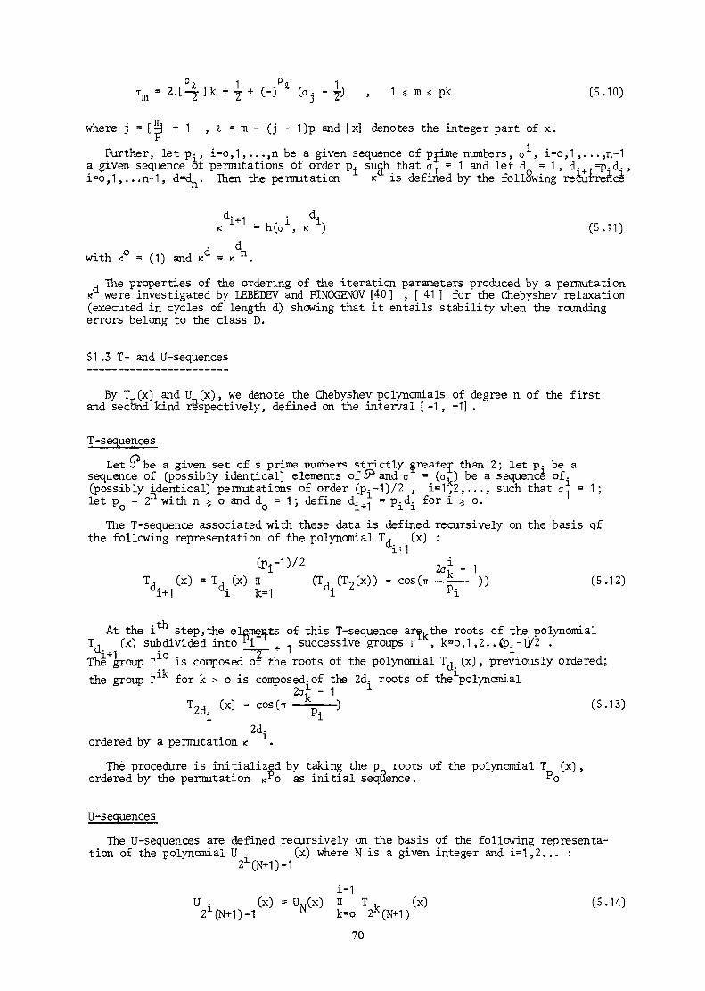
Tm 2.[-|]k + \ + (-) (a. - j) , 1 s m g pk (5.10)

where j = [ 5 +1 , J, = m - (j - 1)p and [x] denotes the integer part of x.

Further, let p., i=o,1,...,n be a given sequence of prime numbers, o1, i=o,1,...,n-1a given sequence of permutations of order p. such that a- = 1 and let d = 1 , d.+ 1=p-d- ,i=o,1,...n-1, d=d^. Then the permutation < is defined by the following recurrence

K 1+1 = hCa1, < ^ (5.11)

A d

with < = (1) and *a = K n.

j The properties of the ordering of the iteration parameters produced by a permutationK were investigated by LEBEDEV and FINOGENOV [40 ] , [ 41 ] for the Chebyshev relaxation(executed in cycles of length d) showing that it entails stability when the roundingerrors belong to the class D.

51 .3 T- and U-sequences

By T (x) and U (x), we denote the Chebyshev polynomials of degree n of the firstand second kind respectively, defined on the interval [ -1, +1] .

T-sequences

(possibly identical) permutations of order (p--1)/2 , 1=1,2,...let p = 2n with n >, o and d = 1 ; define d.+, = p^d. for i ^ o.

The T-sequence associated with these data is defined recursively on the basis ofthe following representation of the polynomial T^ (x) :

(Pi-0/2 fci . ,(x) = T (x) n (T, (T2(x)) - COS(TT ~£ —— )) (5.12)

di k=1 di Z pi

At the i step,the elemeats of this T-sequence are^the roots of the polynomial(x) subdivided into "i + - successive groups r , k=o,1,2..(p.-1^2 .

The group r10 is composed of the roots of the polynomial T^_ (x) , previously ordered;the group rlk for k > o is composed.of the 2d. roots of the1polynomial

9^1 _ 1 1

T,

2ak -(x) - COS(TT — ~— ) (5.13)

2d.ordered by a permutation K

The procedure is initialized by taking the pQ roots of the polynomial T (x) ,ordered by the permutation K*O as initial sequence . PO

U-sequences

The U-sequences are defined recursively on the basis of the following representa-tion of the polynomial U . (x) where N is a given integer and 1=1,2... :

21(N+1)-1

1-1U - (x) =UN(x) n T, (x) (5.14)

Z^N+D-I N k=o 2K(N+1)70

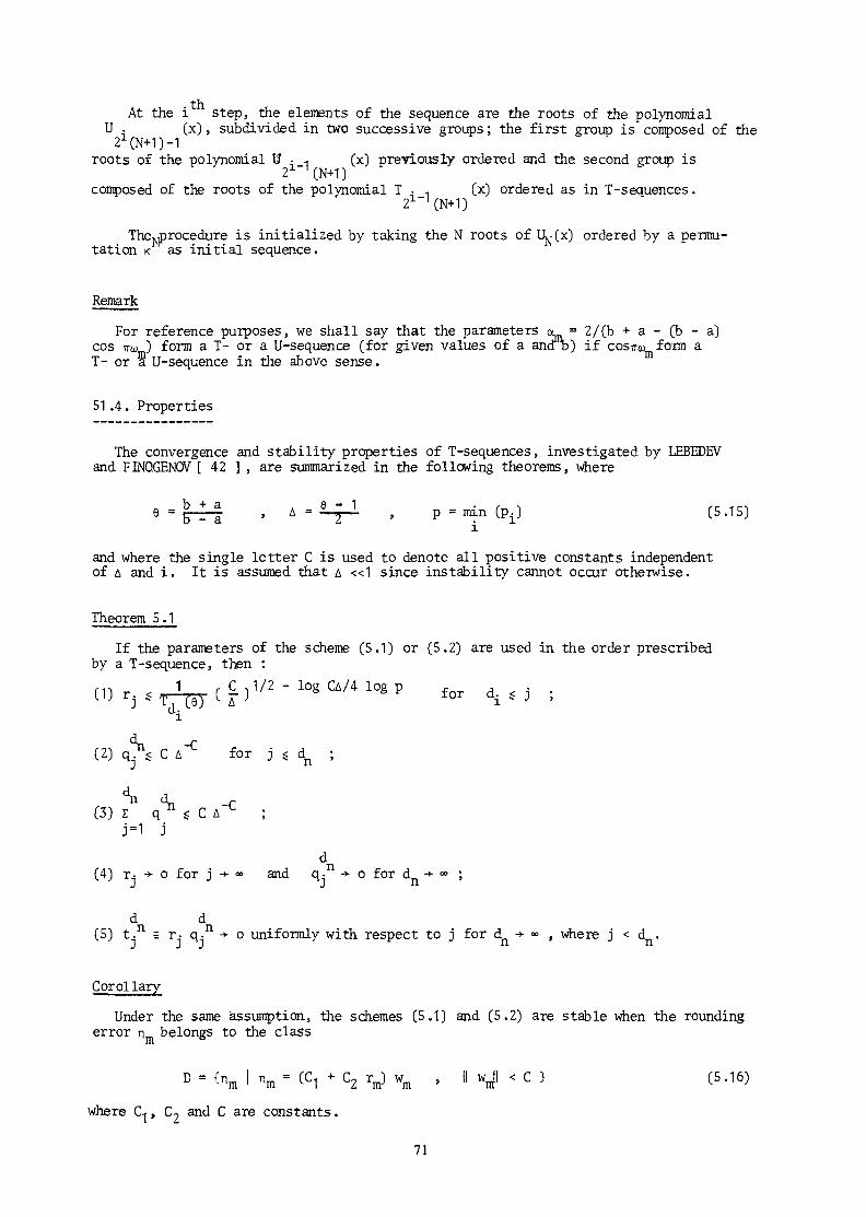
• ~ iAt the i step, the elements of the sequence are the roots of the polynomialU - (x) , subdivided in two successive groups ; the first group is composed of the21(N+1)-1

roots of the polynomial U . 1 (x) previously ordered and the second group is21~'(N-Kl)

composed of the roots of the polynomial T -, (x) ordered as in T-sequences.1 ~ ' -

The>jprocedure is initialized by taking the N roots of UN(X) ordered by a permu-tation K as initial sequence.

Remark

For reference purposes, we shall say that the parameters « = 2/(b + a - (b - a)cos TTU ) form a T- or a U-sequence (for given values of a ando) if cos™ form aT- or a U-sequence in the above sense .

51 .4 . Properties

The convergence and stability properties of T-sequences, investigated by LEBEDEVand FINO.GENÖV [ 42 ] , are summarized in the following theorems, where

e-]~-f . A'^-T1 . p = min (Pi) C5.15)

and where the single letter C is used to denote all positive constants independentof A and i. It is assumed that A «1 since instability cannot occur otherwise.

Theorem 5 . 1If the parameters of the scheme (5.1) or (5.2) are used in the order prescribed

by a T-sequence, then :

d r(2) q.n£ C A~L for j s à ;

J n

(3) z"" qdn « C A~C ;j=1 J

d(4) r• ->• o for j -v oo and q-n ->• o for d -> °° ;

d d(5) t.n = r- q.n -v o uniformly with respect to j for dn -»- » , where j < d .

Corollary

Under the same assumption, the schemes (5.1) and (5.2) are stable when the roundingerror n belongs to the class

where C,, C7 and C are constants.I h

71

Similar assertions can be proved for U-sequences . When 9 = {3 } the followingrefined estimates have been obtained [ 42] :

Theorem 5 .2

If the parameters of the scheme (5.1) or (5.2) are used in the order prescribedby a T-sequence for which y = {3} , then

d TdC2) * C A" -

n

(3) »itK C - 0

51.5. Remark

It was also shown by LEBEDEV [ 35] that the proper ordering of the relaxation para-meters may significantly increase the convergence rate of the method of alternatingdirections in the non-commutative case. This effect is not connected with computatio-nal stability; a qualitative explanation is suggested in [ 35] but no satisfying theo-retical justification has yet been proposed.

5.2. Second order schemes

52.1 . Formalism

Polynomial relaxation of the iterative method (2.2} for solving (2.1) may also beimplemented as a second order iterative method; it can be formulated as the followingmodification of the scheme (2.2):

V1 = xm +

or as the following modification of the residual scheme (2.7)

~1 (Axm '

with 81 = °; again, the choice should be done so as to minimize the computationalwork per iteration.

In the absence of rounding errors, the error evolution is given by

where e = x^ - x, ^(u) is the polynomial of degree m defined by the recurrencerelation

= C1 -

with R0(u) = 1 , and Pm(t) = RÔ - t) .

72

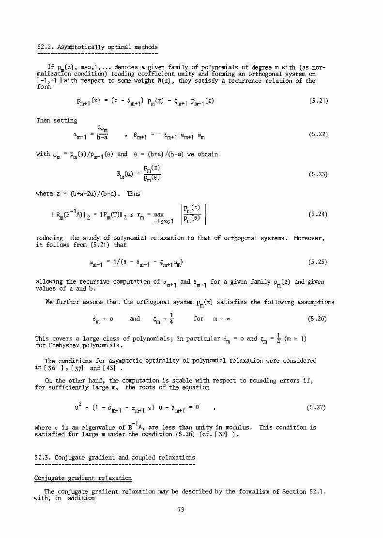
52.2. Asymptotically optimal methods

If Pm(z), m=o,1,... denotes a given family of polynomials of degree m with (as nor-malization condition) leading coefficient unity and forming an orthogonal system onf-1,+1 ]with respect to some weight W(z), they satisfy a recurrence relation of theform

Then setting

V-t = E=a

with Ujn = Pm(9)/Pm+iCe) and 6 = (b+a) /(b-a) we obtain

where z = (b+a-2u)/(b-a). Thus

(5.24)

reducing the study of polynomial relaxation to that of orthogonal systems. Moreover,it f nil nw<; frnm (K . 211 thatit follows from (5.21) that

allowing the recursive computation of a , and g , for a given family p (z) and givenvalues of a and b . m m ' m

We further assume that the orthogonal system Pm(z) satisfies the following assumptions

6 -»• o and ç -*• j for m -»• « (5 .26)

This covers a large class of polynomials ; in particular 6 = o and JL. = T (m > 1 )for Chebyshev polynomials .

The conditions for asymptotic optimality of polynomial relaxation were consideredin [36 ] , [37] and [43] .

On the other hand, the computation is stable with respect to rounding errors if,for sufficiently large m, the roots of the equation

»'-d-ß^-^vDu-ß^-O , (5.27)

where v is an eigenvalue of B A, are less than unity in modulus. This condition issatisfied for large m under the condition (5.26) (cf. [37] ) .

52.3. Conjugate gradient and coupled relaxations

Conjugate gradient relaxationThe conjugate gradient relaxation may be described by the formalism of Section 52.1 .

with, in addition73

Vl = % - Ym = - Y m *

where YQ = o and rm = 5jn/am 6m_1 f or m * 1 and

5 m ' - sj sm) um = (Of V1 sm| B-1A sm)/6m

(5.29)b) -xm)

(x|y) denotes the scalar product and Z is a positive integer. The method minimizesthe following norm of the error at each step

-1 ."KejCB Vcjl (5.30)

under the condition that the error evolution satisfies (5.1 9) where Rm(u) (or pmCt)îs a polynomial of degree m such that ïL(o) = 1 CpmC1) = 1) > the classical theory uusesa = 1 ; the minimization of the euclidian norm of s , obtained with A = 2, is used in,WACHSPRESS [ 57 ] ; we refer to AXELSSON f 3 ] f or a recent account of the theory.

The polynomials R (u) generated by this method form an orthogonal system with res-pect to the weight function

W(u) = I c2 UA 6(u - v.) (5.31)1=1

iwhere v- are the eigenvalues of B A and c- the coefficient of the development of theinitial error

in an orthonormal system {w } of eigenvectors of B A; the interval of definition ofthis weight function may thus be taken as any interval! o. ,ß] such that c- 0 =*v- G [a, ß.] ; it needs not contain all eigenvalues of B A.

The sensitivity of the conjugate gradient relaxation to rounding errors was inves-tigated by LEBEDEV [ 39 1 in the case of Problem I of Section 7 .1 . In particular, Lebedevreports the following result [39 ] : assume that the coefficients of the conjugate gra-dient method can be determined exactly, by use of (5.28) - (5.29) in the absence ofrounding errors; then it is possible to determine a specific problem (of this type)_-|andan initial approximation x such that, for sufficiently small v,/v , we have I'R B A)IL> Cr where C is an arbitrarily large positive constant.

The reasoning of LEBEDEV uses x such that the expansion (5.32) of e involves onlyv- G [ v1 , v /2] ; then Rm(t) is shown to have large amplitude near v_. This result con-firms empirical observations reported by MJTISHAUSER and by GINSBURG in [ 28 ] .

Coupled method

Coupling Chebyshev and conjugate gradient relaxations has been considered in 1 33 ][ 28 ] [ 57 ] [ 3 ] • A new approach was developed by LEBEDEV [37 ] , based on the possi-bility of obtaining information on the boundaries of the spectrum (as well as on thecomponents of the initial error) from the conjugate gradient parameters ; it is thus pro-posed to use conjugate gradient relaxation during a first stage and Chebyshev relaxationduring a second stage, the Chebyshev parameters being estimated from the informationobtained during the first stage.

The resulting algorithm runs as follows : (1) perform a iterations with conjugategradient relaxation; (2) determine the lowest and largest roots, a and b of R (t),defined by (5.20); set e^ = (b^ + a J/fb. - a ) ; (3) use polynomial relaxation with8 = 9 , 6 = o, | = 1/4, i.e. Chebyshev relaxation with 6 = 6 .

jL lU Ti Jo

74

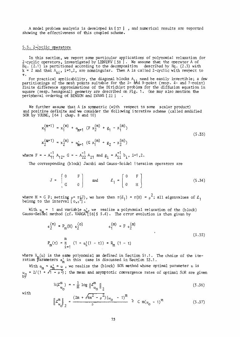
A model problem analysis is developed in [ 37 1 , and numerical results are reportedshowing the effectiveness of this coupled scheme.

5.5., 2-eyelie ope rators

In this section, we report some particular applications of polynomial relaxation for2-cyclic operators, investigated by LEBEDEV [ 38 1 . We assume that the operator A ofEq. (2.1) is partitioned according to the decomposition described by Eq. (2.3) withk = 2 and that A . - , i=1,2, are nonsingular. Then A is called 2-cyclic with respect toIT .

For practical applicability, the diagonal blocks A., need be easily invertible; a fewpartitionings of the mesh points suitable for the S- and 9-point (resp. 4- and 7-point)finite difference approximations of the Dirichlet problem for the diffusion equation insquare (resp. hexagonal) geometry are described on Fig. 1 . One may also mention theperipheral ordering of BENSON and EVANS [ 22 ]

We further assume that A is symmetric (with respect to some scalar product)and positive definite and we consider the following iterative scheme (called modifiedSOR by YOUNG, [64 ] chap. 8 and 10)

,(m+1) = (m) +

(m+1) = (m)2 2

,(m).

fG (m) (m),l 1 g2 X2 J

(5 .33)

where F = - A!.. G = - and gi ^ b. , i=1 ,2.The corresponding (block) Jacobi and Gauss-Seidel iteration operators are

J = 0G

F0

andFH

(5.34)

where H = G F; setting p= r£J), we have then r(JC-) = r(H) = p ; all eigenvalues of £,belong to the interval [o,p 1 .With a = 1 and variable ol, we realize a polynomial relaxation of the (block)

Gauss-Seioel method (cf. VARGA L56]§ 5.4) . The error evolution is then given by

= F (m)

(5.35)- t)) = - t)

where Rm(u) is the same polynomial as defined in Section 51 .1 . The choice of the ite-ration parameters a' in this case is discussed in Section 53.1.

With a = otl = u , we realize the (block) SOR method whose optimal parameter M isto = 2 / ( 1 + /1 - p 2) ; the mean and asymptotic convergence rates of optimal SOR are givenby

' - I 1(*with

'o "2

(2m + Am2 - p 2)(W n - 1)m

* C

(5.36)

(5.37)

75

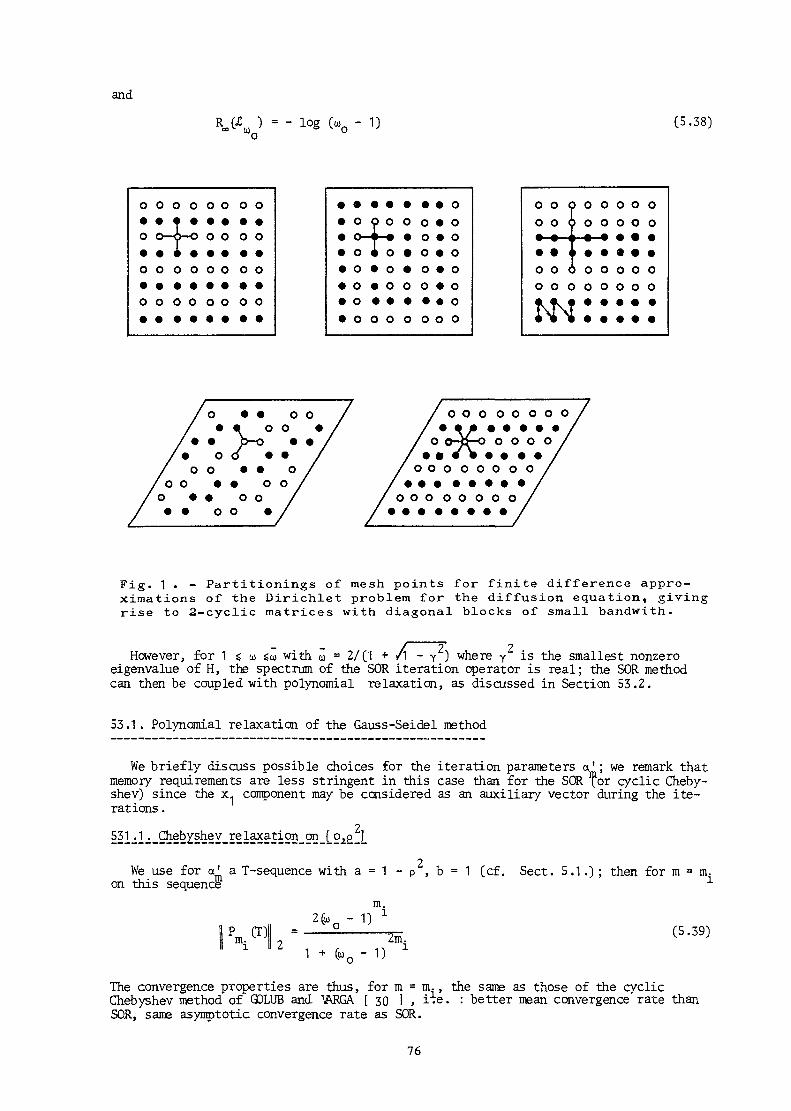
and

Ro=(^ - - 10S(5.38)

o

o•o

o

o o o

o— o— o• • •o o o

o o o

o

0•o

o

o

0•o

o

o

o•o

o

o

0•o

0

o0-0oooo

o o o~T~* *1 0 •• o •• 0 0• • •o o o

ooooo•o c

0oooo0o

> 0

o0•-

0o

r

oo-•-

oo

f

o oT °i •-

0 O

0 0<:

0

o

o0

oo•

oo

0

o•

0

o

o0•

00

o • • o o• • 00 •

o o o o o o o o

o o-u—o o o o o• » • «

o o o o o o o o

o o o o o o o o

Fig. 1 . - Partitionings of mesh points for finite difference appro-ximations of the Dirichlet problem for the diffusion equation, givingrise to 2-cyclic matrices with diagonal blocks of small bandwith.

with u = 2/(1 + /1 - y ) where y is the smallest nonzeroHowever, for 1 s u ueigenvalue of H, the spectrum of the SOR iteration operator is real; the SOR methodcan then be coupled with polynomial relaxation, as discussed in Section 53.2.

53.1 . Polynomial relaxation of the Gauss-Seidel method

We briefly discuss possible choices for the iteration parameters a'; we remark thatmemory requirements are less stringent in this case than for the SOR for cyclic Cheby-shev) since the x. component may be considered as an auxiliary vector during the ite-rations .

We use for a' a T-sequence with a = 1 - p , b = 1 (cf. Sect. 5.1 .) ; then for m = m.on this sequence 1

P OOllV h

m.- D X

(o)0 - D2m. (5.39)

The convergence properties are thus, for m = m., the same as those of the cyclicChebyshev method of CDLUB and 1MGA [ 30 ] , i-e. : better mean convergence rate thanSOR, same asymptotic convergence rate as SOR.

76

The first iteration is performed with a J = 1 and cancels the error projection onthe kernel of H (which may be multidimensional) ; then we use for a ' a T-sequence witha = 1 -p , b = 1 - y > where 0 3 Y $ Y • For m = m- +1 we have tnen

Pmrai+1

I 2 - 2

"with

The convergence properties are (asymptotically) better than those of cyclic Chebyshev;on the other hand, for large numbers of iterations, it is recommended to cancel againthe error projection on the kernel of H, resulting from rounding errors.

Two parameters must be estimated for the second choice; other possibilities usingal = 1 and weighted optimal relaxations on [ o, p ] are discussed in [ 38 ] .

53.2. Coupled SOR and polynomial relaxation

The iteration scheme is modified in

x(m+1) = x(m) + Y^C£ (m) + h _ x(m)} (5>41)

where £ is the SOR iteration operator (deduced from (5.33) with a = a' = a>) ,h = (D - uE) cub where D is the (block) diagonal and -E the (block) lower triangularpart of A, and y +1 are the polynomial relaxation parameters .

In the range 1 s o> * ü, the spectrum of £ is composed of the point 1 -u and theinterval [ n - i ( u ) > n 7(10) ] where n • (u) , i=1,2 are the roots of the equation

I *- 1

1/2 + u - 1 =0 (5.42)n - pa>n

For u= ta, we know in addition that u - 1 G [n 1,19] is an eigenvalue of £- associa-ted with an elementary divisor of the second order. u

These observations lead to the following possible choice for j with u = u : forthe first three iterations, we use

Y! = ü -1 Y2 = Y3 = (2 - w)~1 ; (5.43)

for Y , m > 3, we use a T-sequence associated with a = 1 - n -(N) > b = 1 - n, (ü) ;then ?or m = nu + 3,

? _P ni (u)1 ————— (5.44)(1 -

The convergence properties are (asymptotically) better than those of cyclicChebyshev and also better than those of the methods of Sect. 53.1 . For large numbersof iterations, it is also recommended to repeat from time to time the cycle of thethree iterations (5.43).

77

6. THE ESTIMATION OF ASYMPTOTIC CONVERGENCE RATES

Motivation.

The estimation of asymptotic convergence rates was developed with two purposes :the analysis of model problems and the optimization of relaxation parameters.

In the framework of factorization iterative methods, model problem analysis isneeded to investigate wether the increased computational complexity of higher ordermethods does not offset their increased asymptotic convergence rates, as well as toappreciate the effect of standard relaxation techniques (polynomial relaxation).

On the other hand, the optimal use of factorization iterative methods requires thedevelopment of adequate relaxation techniques and their optimization. The relativeperformances of a few possibilities have been explored for model problems. Presently,the best results have been obtained with optimal diagonal-Chebyshev relaxation.

In this section, we follow the general notation of Section 2.1 . but we considerpoint methods only; thus A, B, C and T are considered as nxn matrices with scalarentries.

Techniques of estimation

Several techniques have been considered, arising from the works of GARABEDIAN [29 3 ,VARGA [ 56 ], PARTER [47] , PRICE and VARGA [48 ], and from Fourier analysis. In morespecific cases, we can also use the result of Theorem 3.9 above and the AXELSSON-GUSTAFSSON [ 4 1 [31 J analysis of diagonal relaxation.

Basically, these estimates can be gathered in two classes. The first one consistsin estimates based on the consideration of the numerical range of the iteration matrixand it is particularly appropriate when the matrix B of the splitting A = B - C whichdefines the iterative scheme, is symmetric and positive definite. The second class(Garabedian estimates) arose from regarding the iterative technique as a discrete time-dependent process, the analysis of which gives estimates for the decrease of variouscomponents of the error; the slowest one gives an estimate of the asymptotic convergen-ce rate; these estimates seem, appropriate for unsymmetric techniques.

In this section, we develop the main ideas, trying to keep the assumptions at ageneral level. More accurate results, which require more detailed assumptions (inpresent formulation at least), will be reported in the next section.

6.1. Numerical range estimates

61.1. Introduction and notations

When A and B are symmetric (hermitian in the complex case)and B is positive definite,the convergence properties of the iterative method defined by the splitting A = B - C,with or without polynomial relaxation, are governed by lower and upper bounds forthe ratios (z Cz)/(z|Bz) or (z[Az)/(z|Bz) where z is an arbitrary non-zero complex n-vector and (x y) denotes the scalar product, i.e. by lower and upper bounds for theToeplitz numerical ranges of the pencils C - tB or A - vB.

We again denote by T. (resp. v^) ,_i=1,2. . .n , the eigenvalues, ordered by increasingalgebraic values, of the matrix T = B C (resp. I - T = B~ A) ; thus T- = 1 - \> _• ,

(z|Cz) (zlAz) ft- «•,C6<1)

and the spectral radius of the iteration matrix T is given by

r(T) = m a x C l ^ l , rj (6.2)

78

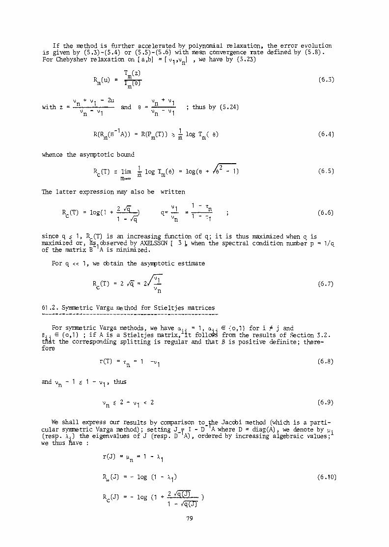
If the nBthod is further accelerated by polynomial relaxation, the error evolutionis given by (5.3)-(5.4) or (5.5)-(5.6) with mean convergence rate defined by (5.8).For Chebyshev relaxation on [a,b] = [v , ,v ] , we have by (5.23)

v + v1 - 2u v -i- v1with z = — —— • ——— and 9 = — ——— - ; thus by (5.24)

- -

R(Rm(B"1A)) = R(Pm(T)) >, 1 log Tm( e) (6.4)

whence the asymptotic bound

RC(T) = lim 1 log Tm(9) = log(e + /Q2 - 1) (6.5)

The latter expression may also be written

RC(T) , logtl . i^__, „. !i , ilia ; C6.6,

since q $ 1, R_(T) is an increasing function of q; it is thus maximized when q ismaximized or, as, observed by AXELSSCN [ 3 \ when the spectral condition number p = 1/qof the matrix B A is minimized.

For q « 1 , we obtain the asymptotic estimate

\(T) = 2 y^= 2 (6.7)

61 .2. Symmetric Varga method for Stielt jes matrices

For symmetric Varga methods, we have a.. = 1, a.. € {0,1} for i ^ j andß. . e {o,1} ; if A is a S tie It jes matrix, """it follows from the results of Section 3.2.tnat the corresponding splitting is regular and that B is positive definite; there-fore

r(T) = tn = 1 -v1 (6.8)

and v - 1 $ 1 - vi , thus

vn $ 2 - V1 < 2 (6.9)

We shall express our results by comparison to_the Jacobi method (which is a parti-cular symmetric Varga method) ; setting J_? I - D A where D = diag(A) , we denote by p-(resp. x.) the eigenvalues of J (resp. D A), ordered by increasing algebraic values;1

we thus Aave :

r(J) - un = 1 - X1

RJJ) = - log (1 - X.,) (6.10)

RC(J) = - log (1 *

79

X1with q(J) = — , andn

0 g 2 - (6.11)

We shall further assume that X« « X since it is only in that case that usualiterative methods become slow and need acceleration. Then we have

ATRc(j) * 2/J- = oc/rpn

(6.12)

Letting A = B - C and T = B~ C be the splitting and the iteration matrix associatedwith some symmetric Varga method, we have

k X, D C(6.13)

1

where k = 1/11 D Cl l 7 and where we have assumed X-, « II D Cl!Similarly L '

max f .1 + Cmin C T C )

n

(6.14)

Since diag(C) = o for Varga methods, it is clear that min /nn^ s 0; thus we have

k1 <: 2 - v- (6.15)

Therefore

R, (T) >, k X1

RC(T) >, 2/^ln

(6.16)

Remarks

(1) We recall that for Stielt jes matrices, the optimal SOR method (which is a parti-cular unsymmetric Varga method with diagonal relaxation) has an asymptotic convergencerate

R (JE ) = max R (JE ) ,~ >t u °° u

(6.17)

where X is the SOR iteration matrix, satisfying

R (6.18)

80

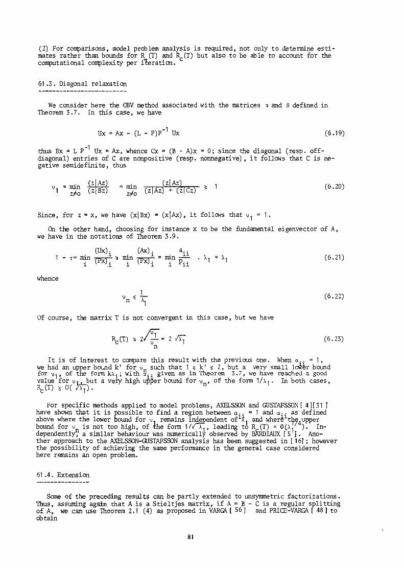
(2) For comparisons, model problem analysis is required, not only to determine esti-mates rather than bounds for R (T) and RC(T) but also to be able to account for thecomputational complexity per iteration.

61.3. Diagonal relaxation

We consider here the GBV method associated with the matrices a and 8 defined inTheorem 3.7. In this case, we have

Ux = Ax - (L - P)P~1 Ux (6.19)

thus Bx = L P Ux = Ax, whence Cx = (B - A)x = 0; since the diagonal (resp. off-diagonal) entries of C are nonpositive (resp. nonnegative), it follows that C is ne-gative semidef inite , thus

» , ' - g ' - J ( l w ' ' (6'20)

Since, for z = x, we have (x|Bx) = (x|Ax), it follows that v1 = 1 .

On the other hand, choosing for instance x to be the fundamental eigenvector of A,we have in the notations of Theorem 3.9.

(Ux). (Ax). au1 - T= min re • v • * min n -, •• = min - — . X-, = X-, (6.21)

i l .i i l Ji i yii

whence

vn , i- (6.22)

Of course, the matrix T is not convergent in this case, but we have

RC(T) 5 2/ —= 2 /Xj (6.23)n

It is of interest to compare this result with the previous one. When a.. = 1,we had an upper bound k' for v such that 1 g k' s 2, but a very small lower boundfor v1, of the form kX 1 ; with a-, given as in Theorem 3.7, we have reached a goodvalue for V1 , but a very high upper bound for v„, of the form 1/Xi . In both cases,Rr(T) >, 0( 7x7). n

U l

For specific methods applied to model problems, AXELSSON and GUSTAFSSON [ 4][31 ]have shown that it is possible to find a region between a.- = 1 and a-, as definedabove where the lower bound for v1 remains independent ofx;L and where the.upperbound for v is not too high, of the form I// x.., leading to R (T) = 0(xJ7 ). In-dependently, a similar behaviour was numerically observed by BAKDIAUX [5 ]. Ano-ther approach to the AXELSSON-GUSTAFSSON analysis has been suggested in [ 16]; howeverthe possibility of achieving the same performance in the general case consideredhere remains an open problem.

61.4. Extension

Some of the preceding results can be partly extended to unsymmetric factorizations.Thus, assuming again that A is a Stieltjes matrix, if A = B - C is a regular splittingof A, we can use Theorem 2.1 (4) as proposed in VARGA [ 56] and PRIŒ-VARGA [ 48 ] toobtain

81

$ — — — — — — C6.24)

~ 1+ii7¥;*• _1

with the notation of Section 61.2. Assuming again that X1 « || D C|l 7, we have asympto-tically '

R^CT) % kx1 with k = 1/|ID~1CII2 . (6.25)

Vfe further note that k may be estimated using Schur's lemma, giving

k% Q|D~1C|I IID"1Cftj"1/2 (6.26)

6.2. Garabedian estimates

The technique we consider now was first introduced by GARABEDIAN [29 ] for analy-zing the SOR method applied to the 5-point finite difference approximation for thePoisson equation in 2-dimensional rectangular geometry. It was used by DE MEERSMAN[ 26 ] for analyzing the SOR method applied to finite difference approximations of thesame equation in hexagonal geometry. A more general formulation was developed byBEAUWENS [13 ] for the analysis of first order iterative methods under specific assump-tions on the asymptotic behaviour of the error and of the matrix B (of the splittingA = B - C which defines the method) for consistent finite difference approximations ofthe d-dimensional Poisson equation; a more rigorous derivation of the latter approachwas given by STANKIEWICZ [ 53 ] .

To summarize the results, we consider a consistent finite difference approximationon a uniform mesh of size h

of the Poisson equation in a d-dimensional region R with homogeneous Dirichlet condi-tions on its boundary r ,

- Au(x) = f (x) x € R(6.28)

u(x) =0 x e r

where x = (x^), i=1,2...d.

We assume that the discrete equation is solved by the first order iterative method

- C ^ u W U b ^ (6.29)

where B. is nonsingular and A, = B, - G , with iteration matrix T, = BT C, .We further assume that

dB, ->• b + h Z b- |H- for h -»• o (6.30)n. o - - i oX-

where b-, i=o,1,2... d are d+1 parameters, independent of x.

82

Then, if TV is an eigenvalue of T, associated with the eigenvector v^, we have

Bh -

and, by the consistency assumption, A, v, = 0(h ), whenever v, is the discrete repre-sentation of a sufficiently smooth function. Therefore, one nas to assume (1 - t , )b0(h ) and two cases may be distinguished :

(a) b0 = 0(1) 1 - Th = och<)

00 - Th - oooUnder these assumptions, the analysis shows (cf. STANKIEWICZ [53 ]) the existence

of a vector <j>, such that

b2) Hh =- O(hm) (6.32)

with m = 5 in case (a) , m = 3 in case (b) .

t"h 9 "?Letting «t^ be the eigenvector of A, associated with its l eigenvalue Ah

(ordered by increasing values)

\ (6.33)

e,following approximate relation is obtained between eigenvalues T, of T, andM h

1 £ u2, (6.34)

This relation has been established under the assumption that the eigenvector v,associated with T, is smooth enough to have A, v, = 0(h ) and it can be seen from thetransformations performed (cf. [ 53 ] ) that it is valid only for the eigenvalues of A,close to zero.

When this smoothness assumption is satisfied for the eigenvector of T, associatedwith the eigenvalue T, of largest modulus, we obtain the following estimates for theasymptotic convergence rate :

2 b

if b > A (2 b)

if b2 = A2!!2 (S_ b?)

if b2 < A 2 (ï b2)

where A.h is the smallest eigenvalue of A, .83

(6.35)

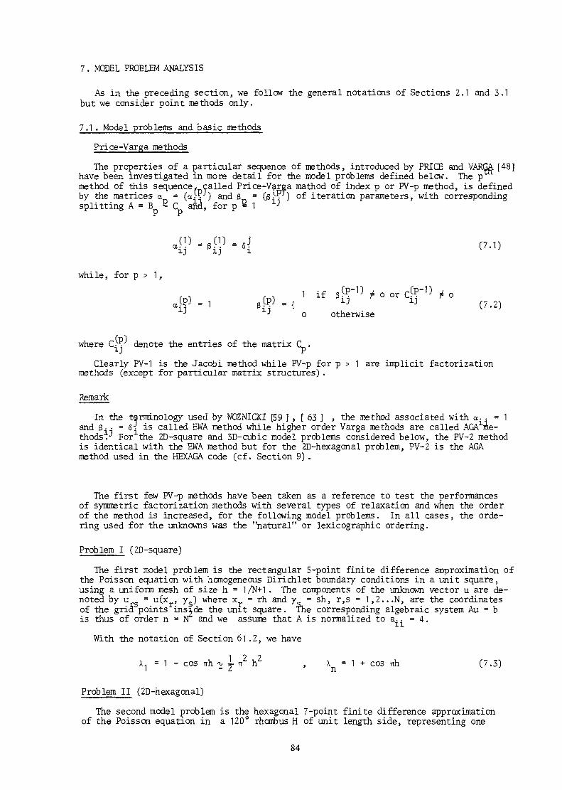
7. MODEL PROBLEM ANALYSIS

As in the preceding section, we follow the general notations of Sections 2.1 and 3.1but we consider point methods only.

7.1 . Model problems and basic methods

Price-Varga methods

The properties of a particular sequence of methods, introduced by PRICE and VARGA [48]have been investigated in more detail for the model problems defined below. The pmethod of this sequence, called Price-Varga mathod of index p or PV-p method, is definedby the matrices a = (a>? J) and 8 = (g- - ) of iteration parameters, with correspondingsplitting A = B * C and, for p B 1

(7.1)

while, for p > 1,

a i j - 1 1 if= {

f o or d?'

otherwise(7.2)

where denote the entries of the matrixClearly PV-1 is the Jacobi method while PV-p for p > 1 are implicit factorization

methods (except for particular matrix structures).

Remark

In the terminology used by WOZNICKI [59 ] , [ 63 ] , the method associated with a-. = 1and ß. - =5- is called EWA method while higher order Varga methods are called AGA me-thods. Forxthe 2D-square and 3D-cubic model problems considered below, the PV-2 methodis identical with the EWA method but for the 2D-hexagonal problem, PV-2 is the AGAmethod used in the HEXAGA code (cf. Section 9) .

The first few PV-p methods have been taken as a reference to test the performancesof symmetric factorization methods with several types of relaxation and when the orderof the method is increased, for the following model problems. In all cases, the orde-ring used for the unknowns was the "natural" or lexicographic ordering.

Problem I (2D-square)

The first model problem is the rectangular 5-point finite difference approximation ofthe Poisson equation with homogeneous Dirichlet boundary conditions in a unit square,using a uniform mesh of size h = 1/N+1. The components of the unknown vector u are de-noted by u = u(x , ys) where xr = rh and y = sh, r,s = 1 ,2 . . .N , are the coordinatesof the grid points inside the unit square. The corresponding algebraic system Au = bis thus of order n = w and we assume that A is normalized to a.. =4.

With the notation of Section 61 .2, we have

X.j = 1 - cos irh 1 2 2ir h \ = 1 + cos irhn (7.3)

Problem II (2D-hexagonal)

The second model problem is the hexagonal 7-point finite difference approximationof the Poisson equation in a 120° rhombus H of unit length side, representing one

84

third of a regular hexagon, with homogeneous Dirichlet conditions on its boundary r ,using a uniform mesh of grid lines parallel to the sides, with N interior points oneach grid line. Again we set h = 1/N+1 and we denote the components of the unknownvector u by u = u(xr, zs) where x = rh and z = sh, s=1,2,...N are the coordinatesof the grid points inside the rhombus with respect to oblique axes parallel to thesides. The corresponding- algebraic system Au = b is again of order n = N" and we assu-me that A is normalized to a. . =6.

With the notation of Section 61 .2, we have (cf. STADTER [52 ]) := •]• A2!!2 = 0.6315 Tr2h2 (7.4)

2 ?where A.. = 2.5259 TT is the lowest eigenvalue of the problem

- A<j> = A <j> in H(7.5)

= 0 on r

Problem III (3D-cubic)

The third model problem is the rectangular 7 -point finite difference approximationof the Poisson equation with homogeneous boundary conditions in a unit cube, usinga uniform mesh of size h = 1/N+1 . The components of the unknown vector u are denotedby urst = u^sr» ysj zp where xr = rh, ys = sh, z,. = th, r,s,t = 1.2. . .N, are thecoordinates of the grid points inside the cube . me corresponding algebraic systemAu = b is of order n = N and we assume that A is normalized to a. . = 6 .

With the notation of Section 6I .2, we have

AI = 1 - cos A i 2" ^"- > X = 1 + cos irh (7.6)

Effective convergence rates

To account for the computational complexity per iteration, effective convergencerates have been considered, defined as

R (T) R (T)-ÜOT C o r - ) with

where m (resp . m ) is the number of multiplications per point per iteration of themethod under consideration (resp. of the point Jacobi method) . This is a slight mo-dification of HAGEMAN-VARGA definition [32 1 .

For the model problems : m =4 for Problem I and m = 6 for Problems II and III.

In counting numbers of operations, we use the fact that the diagonal factor P canbe normalized to unity during the iterations and we choose the less expensive schemebetween the direct implementation of (2.2) and the residual scheme (2.7) or between(5.1) and (5.2) in the presence of polynomial relaxation.

7 .2 . Parter-Fourier analysis

For the analysis of unsymmetric relaxation techniques, Garabedian analysis has beenused (cf. below). On the other hand, for symmetric relaxation techniques, the re-sults of Section 6.1 give boundsrather than estimates for v, and v , the lowest andlargest eigenvalues of I - T = B A. They have been supplemented by" the introductionof Parter estimate for v^ and Fourier estimate for v .

85

Parter estimate

The Parter estimate is defined, with the notation of Section 61 .2, by

with

where x is the fundamental eigenvector of the matrix D~ A. It may also be written

For symmetric factorization methods applied to the model problems and associatedwith regular splittings, the analysis of PARTER [47 1 is applicable, showing that thisestimate is asymptotically correct for h -*• o. From numerical results, its range ofapplication appears as much wider, as commented below, though no theoretical justifica-tion has yet been given.

Fourier estimate

Fourier analysis was used by BARDIAUX [5 ] , [ 6 ] , to define the following esti-

(x | Ax.) ia a

mate for v :

°r (x [Ax'a a a. 1 a or

X ' Cx )a1 a.

where x is the vector with components (x ) or (x ) . defined as follows for eachmodel problem a rs a rst

(x )„ = (x.)^ exp (i (itt. + sa9)) for the 2D-square problemCt li 1 LJ l L

(x )rs = exp (i (ra-j + sa2)) for the 2D-hexagonal problem } (7.12)

(xa)rst= ^X1^rst ex? C1 ra1 + Sa2 + tas)}

for the 3D-cubic problem

where (x,) or Cx-t)rst denote the components of the fundamental eigenvalue of D A.In other words the Fourier estimate is the upper bound of the sampling of the numericalrange of the pencil A - vB by Fourier modes modulated^when feasible^by the fundamentalmode of DA.

Heuristic arguments can be developed (cf. BRANDT [ 23 ] for example) to qualitativelyunderstand the effectiveness of Fourier analysis but an accurate theoretical justifi-cation is lacking.

7.3. Numerical results

The numerical results determined for the first 'few PV methods applied to the modelproblems are summarized in Tables I-III, and on Fig. 2. In the Tables, we report ineach case the asymptotic estimate of R^CT) or R_(T) , the number m of multiplicationsper point per iteration and the asymptotic estimate of R„£f (T) . Diagonal relaxation isunderstood with a. - = — ; <D denotes the value of u whicn optimizes this relaxation(independently of any Subsequent polynomial acceleration) . For comparison, the asymp-totic values of the convergence rates of optimal SOR methods are also reported.

86

The convergence rates of PV methods without relaxation have been estimated byBEAUWENS-SURLEZANOSKA [ 19 ] for Problem I, BEAUWENS-STANKIEWICZ [ 18 1 for Problem III,BEAUWENS-WOZNICKI [ 21 ] and BARDIAUX [ 6 ] for Problem II using Parter estimate;Parter theory being applicable in this case, the results are asymptotically correct.Moreover, it was numerically„observed that Parter estimate is accurate, even for lowvalues of r- (errors on R^/ir b/ less than 1 I are reported in [ 19] ,[ 18 ] for PV methodsapplied to Problem I and°°Problem 111, with h = 0.1).

The evaluation of the convergence rates of PV methods with diagonal relaxation, ofthe optimal diagonal factor to and of Chebyshev acceleration has been worked byBARDIAUX [ 5 ] , [6 ]using Parter-Fourier analysis. These results have no theoreticaljustification; however the validity of Parter-Fourier analysis was numerically investi-gated by BARDIAUX [ 5 ]for the PV-2 method applied to Problem I and found very accu-rate for the above mentioned evaluation.

The combined optimization of diagonal and Chebyshev relaxations was also consideredby BARDIAUX [ 5 ] for the PV-2 method applied to Problem I. However, Parter-Fourieranalysis was found less accurate in this range, predicting a Sh behaviour for RC(T) ,in agreement with the results of Axelsson-Gustafsson analysis but not an asymototicallycorrect value for R^fT)// TT h (cf. Fig. 2), the predicted value being approximately 10 \to high.

The convergence rates of PV methods with optimal single overrelaxation were estima-ted by Garabedian analysis for Problem I and II. It was numerically observed thatoscillating error modes prevent the possibility of attaining these optimal convergencerates; however, it was shown possible to reach close values by inserting periodicallyan alternate unrelaxed or underrelaxed auxiliary iteration, the net result being toreduce somewhat the values predicted in Tables I and III (cf. [13 ]) .

Finally, we mention that the use of the double overrelaxation technique was nume-rically investigated in [ 21 ]. Though accurate results are not yet available, thistechnique seems also to give 0(h) asymptotic convergence rates.

To conclude, we remark that, so far, the best results have been obtained with theoptimal combination of diagonal and Chebyshev relaxations as is clearly displayed onFig. 2.

87

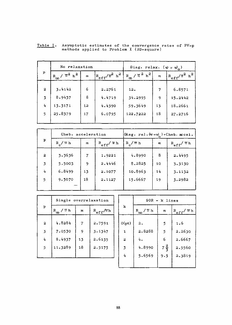
Table I. Asymptotic estimates of the convergence rates of PV-pmethods applied to Problem I (2D-square)

P

2

3

4

5

No relaxation

R o o / ^ h 2

3.4142

8.9437

13.3171

25.8379

m

6

8

12

17

RefX *2

2.276l

4.4719

4.4390

6.0795

Diag. relax. ( <0 = u) )

R / IT2 h2CO

12.

34.2995

59.3649

122.7222

m

7

9

13

18

Reff/TI2 h2

6.8571

15.2442

18.2661

27.2716

P

2

3

4

5

Cheb. acceleration

R /TTh

3.3636

50003

6.8499

9.5070

m

7

9

13

18

Reff / 1 T h

1.9221

2.4446

2.1077

2.1127

EtLag. re l . (<U=u) )+Cheb. accel.

R /TThC

4.8990

8.2825

10.8963

15.6667

m

8

10

14

19

R e f f /TTh

2.4495

3.3130

3.1132

3.2982

P

2

3

4

5

Single overrelaxation

R œ / T T h

4.8284

7.0530

8.4937

11.3-289

m

7

9

13

18

Reff/rrn

2.7591

3.1347

2.6135

2.5175

k

0(pt)

1

2

3

4

SOR - k lines

R / T T hCO

2.

2.8288

4.

4.899O

5.6569

m

5

5

6

't9.5

R e f f /TTh

1.6

2.2630

2.6667

2.5560

2.3819

88

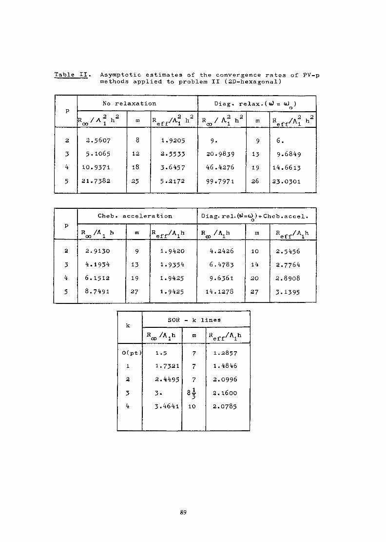
Table II. Asymptotic estimates of the convergence rates of PV-pmethods applied to problem II (2D-hexagonal)

P

2

3

k

5

No relaxation

R /A? h200 1

2.5607

5« 1065

10.9371

21.7382

m

8

12

18

25

RefX h"

1.9205

2.5533

3.6457

5.2172

Diag. relax. ( u) = uJ )

R / A? h2oo 1

9.

20.9839

46.4276

99.7971

m

9

13

19

26

RefX ^

6.

9.6849

14.6613

23.0301

P

2

3

4

5

Cheb . acceleration

Roo /Al h

2.9130

4.1934

6.1512

8.7491

m

9

13

19

27

Reff /Alh

1.9420

1.9354

1.9425

1.9425

Diag. r el. (<i) = u) ) + Cheb. ace el .

R ™ / A i h00 1

4.2426

6.4783

9.6361

14.1278

m

10

14

20

27

Reff /Alh

2.5456

2.7764

2.8908

3.1395

k

0(pt )

1

2

3

4

SOR - k lines

Roo /Alh

1.5

1.7321

2.4495

3.

3.464l

m

7

7

7

8i

10

Reff /Alh

1.2857

1.4846

2.0996

2.1ÔOO

2.0785

89

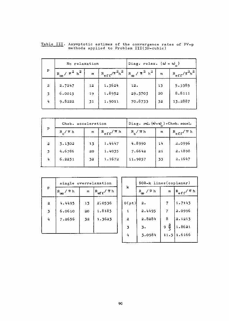
Table III. Asymptotic estimes of the convergence rates of PV-pmethods applied to Problem III(3D-cubic)

p

2

3

4

No relaxation

R / TT2 h200

2.7247

6.0015

9.8222

m

12

19

31

2 2ef f

1.3024

1.8952

1.9011

Diag. relax. (cJ = uj )

R / TT2 h2CD

12.

29.3703

70.8733

m

13

20

32

R /Tt2h2ef f

5.5385

8.8111

13.2887

P

2.

3

k

Cheb. acceleration

R /T" hc

3.1302

4.6786

6.2251

m

13

2O

32

Reff / l t h

1.4447

1.4035

1.1672

Diag. rel. (u)=u) ) +Cheb. accel.

R /TThO

4.8990

7.6642

11.9057

m

14

21

33

Reff / T T h

2.0996

2. 1898

2. 1647

P

2

3

4

single overrelaxation

R / T T hoo

4.4495

6.0610

7.2656

m

13

20

32

R / TT heff

2'.0536

1.8183

1.3623

k

0(pt )

1

2

3

4

SOR-k lines ( coplanar)

R /TTh00

2.

2.4495

2.8284

3.

3.0984

m

7

7

8

> f11.5

Reff /1Th

1.71*3

2.0996

2.1213

1.8621

1.6166

90

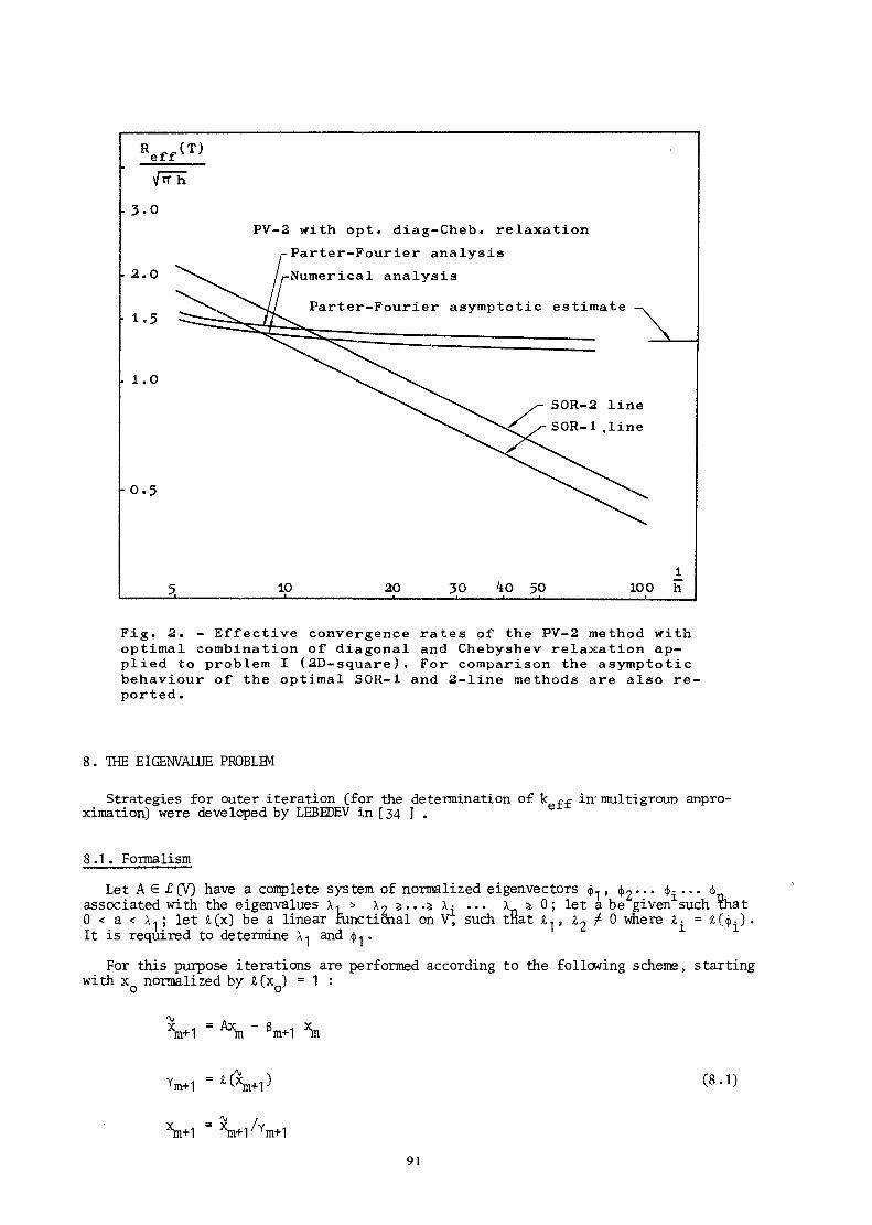
Reff(T)i/rrh

3.0

2.0

• 1.5

1.0

0.5

PV-2 with opt. diag-Cheb. relaxation•Parter-Fourier analysis-Numerical analysis

Parter-Fourier asymptotic estimate

SOR-2 lineSOR-1 .line

10 2O 30 4O 50 100 h

Fig. 2. - Effective convergence rates of the PV-2 method withoptimal combination of diagonal and Chebyshev relaxation ap-plied to problem I (2D-square). For comparison the asymptoticbehaviour of the optimal SOR-1 and 2-line methods are also re-ported.

8. THE EIGENVALUE PROBLEM

Strategies for outer iteration (for the determination of k ff in' multigrour» appro-ximation) were developed by LEBEDEV in [34 1 .

8 .1 . Formalism

Let Ae JEÇV) have a complete system of normalized eigenvectors <fi . , < j > 2 . . . < j > - ... <j>associated with the eigenvalues A., > x2 5...5 X- ... X ^ 0; let a be given such that0 < a < A., ; let A(x) be a linear functional on V, such that i^, k^ £ 0 where a^ = £ ( < j > . ) .It is required to determine X-, and $.. .

For this purpose iterations are performed according to the following scheme, startingwith x normalized by £(XQ) = 1 :

(8.1)

- ^ /xm+1 = xm-(-1/Ym+1

91

for ÏÏF=O, 1,2..,; setting

X — r r~ j, co 9*1m T * (.0 • J

the following relations are readily established

cr = V^Cr1 C8.3)'mn . nn /-ylH/1 » 's ^ J ™ I ,ii vJ « I A • 1 C • (p .

i=1 3 X X X

C8.5)

wherem

= H__ (X - ß^ Pm(X) = (^(X) (8.6)_ _

8.2. Strategies

In [34 ] , LEBEDEV develops the following three-stage stratégie for choosing theparameters ß .

Stage 1 (determination of X. and X„)

One sets ß = £ (1 - cos iru ) where cos ™_ form a T-sequence. It follows fromthe analysis of (5.5) that themcoefficients m c™ are rapidly (resp. optimally) atte-nuated for i 5 2 (resp. for i such that X^ S [ o,a ] ) .

Further, applying i to four successive iterates, using (8.2) and (8.4), and retai-ning only the first two terms., in the summations, one obtains a system of four equationswith unknowns X . , , X 2 > Ci = Ci i - i » c2

= C;? &2' wôse solution gives X., and x„-

This stage is continued until stable values are obtained for x, and X2- Assume thisto occur for m = nu ; assume further that the accuracy on $* is not yet sufficient.

Then, if X2 S a> the procedure is continued until the required accuracy on $« isreached; if X2 > a-, one shifts to stage 2.

Stage 2 (elimination of oj")

A set of four iterations is performed, with ß +.. = X-, 6 ^ ~ ® whüe ß +^ andg +. are determined from an approximate solu- 1 tion \ of the i

t following minimax problem

(x -^ 11L. •

inf max1-3 ' Sm1+4

(8.7)

The corresponding formulas for g +_ and ß +, are given in [ 34 ] ; thecancel the component cT and smooth 1 i the subsequent rounding

are given in [ 34 ] ; these iterationserror.

92

If the required accuracy on <$>* is not yet achieved, one shifts to stage 3.

Stage 3 (determination of (j^)

First variant : return to stage 1 with a = \j-Second variant : taking into account the operations performed during stage 2, a

better way to continue the iterations consists in using g = (A 2/2)0 - cos TtmJ where,for m = nij+4+p, cos KM = cos TTW with cos TUO forming a "-sequence.

Remarks

Two variants of the technique used in stage 1 for the determination of X1 and \2have also been discussed by LEBEDEV (unpublished) :(a) based on the use of two linear functionals l(x), m(x);(b) adapted to the case where the adjoint problem must be solved' simultaneously.

9. CODES

Two codes have been developed for solving the multigroup diffusion approximationof the neutron criticality problem in 2D hexagonal geometry : HEXAGA-II developedby WOZNICKI [60] , [61 1 , [ 62 I and TIP, developed by ARKUSZEWSKI and BORYSIEWÎCZ[1 ] , t 2 ] .

9.1. HEXAGA-II

Three versions, HEXAGA-II-120, -60 and -30 have been developed, differing only bythe geometrical symmetries assumed. In HEXAGA-II-120, the critical problem is solvedon a 1 20° rhombus representing one third of a regular hexagon and logarithmic bounda-ry conditions are accepted on the four boundaries. In HEXAGA-II-60 (resp. -30), a60° (resp. 30°) symmetry is assumed : the problem is solved on a triangle representinghalf (resp. a quarter) of the 120° rhombus with reflecting conditions (zero normalderivative of the flux) on the inner boundaries and logarithmic conditions on the ou-ter boundary.

All three versions, written in Fortran W with dynamic storage allocation, havebeen implemented on IBM 370/168, and CDC-CYBER-73; they use the same input data, theassumed symmetry being checked for in HEXAGA-II-60 and -30.

The method of solution is the usual space-group inner-outer iteration scheme (inneriterations for the spatial equation within each group, outer iteration on the fissionsource, scattering sources being recomputed before entering inner iterations for eachgroup)with discretization by the 7-point finite difference approximation on a uniformtriangular mesh, inner iterations within each group by the PV-2 method (cf. Section7.1) with double overrelaxation (cf. Section 4) and outer iteration by the power me-thod with extrapolation. Empirical formulas are used for the determination of therelaxation factors of the double overrelaxation procedure; the number of inner itera-tions per outer iteration is held fixed for all groups, a (limited) variation withouter iterations being allowed.

The program solves either the direct or adjoint critical problem; it can handleup to 40.000 mesh points with a minimum of 2 and a maximum of 40 energy groups; arbi-trary group to group scattering and fission transfer are allowed, logarithmic bounda-ry conditions may be specified group-wise or point-wise.

We refer to [60] , [62 ] for memory requirements and typical running times. Compa-risons with existing codes reported in BUCKEL et al. [24 ] show that HEXAGA-II isfaster than TRIBU (based on SLOR for the inner iterations), and CITATION (based onalternating-direction line relaxation). further numerical results are reported in [ 65]

93

9.2. TIP

In TIP, the critical problem is solved on the same 30° triangle as in HEXAGA-II-30but logarithmic boundary conditions are accepted on all boundaries.

The program, written in Fortran IV with dynamic storage allocation, has been imple-mented on CDC-CYBER-73.

The method of solution is the same space-group inner-outer iteration scheme as inHEXAGA-II with also the same discretization, but inner iterations use the (block)Gauss-Seidel method for 2-cyclic matrices with Chebyshev relaxation as described inSection 531.1 and outer iterations use the power method with Chebyshev relaxation per-forned according to the Lebedev strategy described in Section 8. The 2-cyclic formis obtained by use of the line red-black ordering.

The program was more recently developed than HEXAGA-II; first experience with anearly version has been reported in [ 2].

10. ACKNOWLEDGMENT

We are happy to acknowledge here the invaluable help of Dr. M. BORYSIEWICZ inpreparing this summary as well as during the development of this cooperation.

REFERENCES

[ 1 ] J. ARKUSZEWSKI and M. BORYSIEWICZ, TIP-1, Users manual, Computing CenterCYFRONET, Swierk (1978).

[ 2 ] j. ARKUSZEWSKI and M. BORYSIEWICZ, "Program TIP for solving the 2D multigroupdiffusion equation in a 30° wedge shaped region", Proceedings of DeutschesAtomforum, Mannheim (1977), pp. 115-118.

[ 3 ] 0. AXELSSON, "Solution of linear systems of equations : iterative methods",Sparse matrix techniques, edited by V.A. Barker, Springer-Verlag (1976), pp.^-^-—————————

[ 4 ] 0. AXELSSON, "A generalized SSOR method", BIT, J3_ (1972) pp. 443-467.[ 5 ] M. BARDIAUX, "Etude sur l'estimation des taux de convergence des méthodes ité-

ratives de factorisation du type FP(k) en présence de relaxation", Rapporttechnique, Université Libre de Bruxelles (1978) .

[ 6 ] M. BARDIAUX, Id. 2ême partie (1979).[ 7 ] F.L. BAUER, "Theory of norms", Technical report CS 75, Stanford University

(1967).[ 8 ] R. BEAUWENS, "Convergence analysis of some factorization iterative methods for

M-matrices", Series in Appl. Math., Rep. 73-7, Northwestern University, Evanston.Illinois (1973).

[ 9 ] R. BEAUWENS, "On the point and block factorization iterative methods for arbi-trary matrices and the characterization of M-matrices"", Series in At>pl. Math.,Rep. 74-1, Northwestern University, Evanston, 111. (1974).

[10 ] R. BEAUWENS, "On the application of relaxation techniques to the factorizationiterative methods", Series in Appl. Math., Rep. 74-3, Northwestern University,Evanston, 111. (1974).

[11 ] R. BEAUWENS, "Semistrict diagonal dominance", SIAM J. Numer. Anal.» 13_ (1976),pp. 109-112.

94

[12 ] R. BEAUWENS, "On a characterization theorem for M-operators", Rep. INR 1693/OTRONET/PM/A, Institute of Nuclear Research, Swierk [1977).

[13 ] R. BEAUWENS, "Garabedian estimates for single relaxation", Technical report,Université Libre de Bruxelles (1977).

[14 ] R. BEAUWENS, "Factorization iterative methods, M-operators and H-operators",Numer. Math.. 31_ (1979), pp. 335-357.

[15 ] R. BEAUWENS, Technical report, in preparation,

[16 ] R. BEAUWENS, "On OBV methods", DOE Report N° COO-2280-38, Northwestern Univer-sity, Evanston, 111. (1979).

[17 ] R. BEAUWENS and L. QUENON, "Existence criteria for partial matrix factorizationsin iterative methods", SLAM J. Numer. Anal., ]3_ (1976), pp. 615-643.

[ 18 ] R. BEAUWENS and R. STANKIEWICZ, "On single-stage iterative methods forsolving three dimensional diffusion problems", Rapport technique, UniversitéLibre de Bruxelles, Bruxelles (1976) .

[ 19 ] R. BEAUWENS and S. SURLEZANOSKA, "Sur les taux de convergence asymptotiquesdes méthodes itératives de factorisation", Rapport technique, UniversitéLibre de Bruxelles, Bruxelles (1976).

[ 20 ] R. BEAUWENS and J.J. VAN BINNEBEEK, "Convergence theorems in Banach algebras",Pacif. J. Math., 68_ (1977), pp. 13-24.

[ 21 ] R. BEAUWENS and Z. WOZNICKI, "Model problem in hexagonal geometry", Statusreport, unpublished (1977).

[ 22 1 A. BENSON and D.J. EVANS, "Successive peripheral over-relaxation and otherblock methods", J. Comput. Phys., 2J_ (1976) pp. 1-19.

[ 23 ] A. BRANDT, "Multi-level adaptative solutions to boundary value problems",Math. Comp.. 31_ (1977) pp. 333-390.

[ 24 l G. BUCKEL, K. KUFNER and B. STEHLE, "Benchmark calculations for a sodium-cooled breeder reactor by two- and three-dimensional diffusion methods",Nucl. Sei. Eng., 64_ (1977) pp. 75-89.

[ 2 5 ] N.I. BULEEV, "A numerical method for the solution of two-dimensional andthree-dimensional equations of diffusion", Mat ._Sb . , 51 (1960) pp. 227-238;English transi. Rep. BNL-TR-551, Brookhaven National laboratory, Upton, NewYork (1973).

[ 2 6 l R. DE MEERSMAN, "The method of Garabedian", Numer. Math.. 1]_ (1968) pp. 257-263

[ 2 7 ] T. DUPONT, R.P. KENDALL and H.H. RACHFORD, "An approximate factorization pro-cedure for solving self-adjoint elliptic difference equations", SIAM J. Numer.Anal.. 5_ (1968) pp. 559-573.

[ 2 8 ] M. ENGELI, Th. GINSBURG, H. RUTISHAUSER and E. STIEFEL, "Refined iterativemethods for computation of the solution and the eigenvalues of self-adjointboundary value problems", Mitteilungen aus dem Institut für angewandte Mathe-matik, nr. 8, ETH, Zürich (1959).

[ 29] P.R. GARABEDIAN, "Estimation of the relaxation factor for small mesh size",M.T.A.C., 10_ (1956) pp. 183-185.

[ 30] G.H. GOLUB and R.S. VARGA, "Chebyshev semi-iterative methods, successiveoverrelaxation iterative methods and second order Richardson iterative methods"Numer. Math., 3_ (1961). Part I pp. 147-156 and Part II pp. 157-168.

[ 31 ] I. GUSTAFSSON, "A class of first order factorization methods", B.I.T., 18(1978) pp. 142-156. ———— ~"~

[ 32] L.A. HAGEMAN and R.S. VARGA, "Block iterative methods for cyclically reducedmatrix equations", Numer. Math., 6_ (1964) pp. 106-119.

95

[33l C, LANCZOS, "Solution of systems of linear equations by minimized iteration",NBS, J. of Res., 49_ (1952) pp. 33-53.

[ 34] V.I. LEBEDEV, "An iterative method with Chebyshev parameters for findingthe maximum eigenvalue and corresponding eigenfunction", Zh. vychisl. Mat, mat.Fiz., 17, 1 (1977) pp. 100-108; Engl. transi. USSR Comput. Math. Math. Phys.,17,1 (1977) pp. 92-101. ———————————————————

[ 35] V.I. LEBEDEV, "On a Zolotarev problem in the method of alternating directions",Zh. vychisl. Mat, mat. Fiz., 17,2 (1977) pp. 349-366; Engl. transi. USSRComput. Math. Math. Phys., 1772(1977) pp. 58-76.

[ 36] V.I. LEBEDEV, "Wsighted optimal iterative methods", Computational methods oflinear algebra (Vychisl. metody lineinai algebry), VTs SO Akad. Nauk SSSR,Novosibirsk (1977).

[37 ] V.I. LEBEDEV, "Iterative methods of solving linear operator equations andpolynomials least deviated from zero" in "Mathematical analysis and relatedmathematical problems", Academy of Science, Novosibirsk (1978).

[38] V.I. LEBEDEV, "Chebyshev methods for solving systems with two-cyclic matri-ces; comparison with the block successive overrelaxation method" in"Finite-difference and variational methods", Vol. 2, Academy of Science,Novosibirsk (1977).

[39] V.I. LEBEDEV, "Game theory and optimal iterative methods", Proceedings ofthe Symposium on differential equations and computational mathematics,Novosibirsk, to appear.

[ 4Qj V.I. LEBEDEV and S.A. FINOGENOV, "Ordering of the parameters in the cyclicalChebyshev iterative method", Zh. vychisl. Mat, mat. Fiz., 11,2 (1971) pp. 425-438; Engl. transi. USSR Comput. Math. Math. Phys.. 11,2 (1971T pp. 155-171 .

[ 41] V.I. LEBEDEV and S.A. FINOGENOV, "Solution of the parameter ordering problemin Chebyshev iterative methods", Zh. vychisl. Mat, mat. Fiz., 1_3j,J_ (1973) pp.18-33; Engl. transi. USSR Comput. Math. Math. Phys., 13, 1 (1973) .pp. 21-42.

[ 43 V.I. LEBEDEV and S.A. FINOGENOV, "Utilization of ordered Chebyshev parametersin iterative methods", Zh. vychisl. Mat, mat. Fiz., 16,4 (1976) pp. 895-907;Engl. transi. USSR Comput. Math. Math. Phys., 16,T (T97F) pp. 70-83.

[43] V.l. LEBEDEV, Yu A. VLASOV and S.A. FINOGENOV, "On asymptotically optimaliterative methods, using information on the spectrum of the operator and onthe decomposition of the initial error, Computational methods of linear alge-bra (Vychisl. metody lineinai algebry), VTs SO Akad Nauk, Novosibirsh (1977) .

[ 44] M. MARCUS and H. M3NC, "A survey of matrix theory and matrix inequalities",Allyn and Bacon, Bos-ton (1964).

[ 45] J.A. MEIJERINCK and H.A. van der VORST, "An iterative solution method for•linear systems of which the coefficient matrix is a symmetric M-matrix",Math. Comput.. 31_ (1977) pp. 148-162.

[ 46] T.A. OLIPHANT, "An extrapolation process for solving linear systems", Quart.Appl. Math., 20_ (1962) prj. 257-267.

[ 47] S.V. PARTER, "On estimating the "rates of convergence" of iterative methodsfor elliptic difference equations", Trans. Amer. Math. Soc., 114 (1965) pp.320-354. ——

[ 48] H.S. PRICE and R.S. VARGA, "Incomplète primitive factorizations", unpublishedmanuscript (1964).

[49 ] L. QUENON, 'Tactorisabilité et convergence des méthodes itératives d'Oliphant-Buleev", Ph. D. Thesis, Université Libre de Bruxelles (1977).

96

[50 ] F. ROBERT, "Recherche d'une M-matrice parmi les minorantes d'un opérateurlinéaire", Numer. Math.. 9_ (1966) pp. 189-199/

[51 ] F. ROBERT, "Blocs-H-matrices et convergence des méthodes itératives classiquespar blocs", Lin. Alg. Appl., 2_ (1969) pp. 223-265.

[52 ] J.T. STÄDTER, "Bounds to eigenvalues of rhombical membranes" J..SIAM Appl. MathU_ (1966) pp. 324-341.

[ 53 ] R. STANKIEWICZ, "On the estimation of the spectral radius of the iterationmatrix", Institute of Nuclear Research, Computing Center CYFRONET, Swierk(1978).

[54 ] H.L. STONE, "Iterative solution of implicit approximations of multi-dimensionalpartial differential equations", SIAM J. Numer. Anal., 5_ (1968) pp. 530-558.

[55 ] R.S. VARGA, 'Tactorization and normalized iterative methods", in "Boundaryproblems in differential equations" edited by R.E. LANGER, Madison, Universityof Wisconsin Press (1960) pp. 121-142.

[56 ] R.S. YARGA, "Matrix iterative analysis", Englewood Cliffs, N.J., Prentice-Hall(1962).

[57 ] E.L. WAOEPRESS, "Iterative solution of elliptic systems and applications tothe neutron diffusion equations of reactor physics", Englewood Cliffs, N.J.,Prentice-Hall (1966).

[58 ] Z. WOZNICKI, Kernenergie,10 (1971) pp. 325-328.

[ 59 ] Z. WOZNICKI, "Two-sweep iterative methods for solving large linear systemsand their application to the numerical solution of multigroup-multidimensionalneutron diffusion equation", Doctoral Dissertation Rep. N° 1447/CYFRONET/PM/A, Institute of Nuclear Research, Swierk (1973).

[ 60 ] Z. WOZNICKI, "HEXAGA-II, a two-dimensional multigroup neutron diffusionprogramme for a uniform triangular mesh with arbitrary group scattering forthe IBM 370/168 computer", Karlsruhe, Gesellschaft für Kernforschung m.b.H.(1976).

[ 61 ] Z. WOZNICKI, "The OLA iterative methods for solving difference equations insymmetrical diffusion reactor problems", Institute of Nuclear Research, Swierk(1976).

[ 62 ] Z. WOZNICKI, "HEXAGA-II-120-60-30 two-dimensional'multigroup neutron diffusionprogrammes for a uniform triangular mesh with arbitrary group scattering",Institute of Nuclear Research, Computing Center CYFRONET, Swierk (1978).

[ 63 ] Z. WOZNICKI, "AGA two-sweep iterative methods and their application in criticalreastor calculations", Nukleonika, 23_ (1978) pp. 941-968.

[ 64 ] D.M. YOUNG, "Iterative solution of large linear systems", Academic Press (1971)

[65 ] J. MIKA and Z. WOZNICKI, "Iterative methods for solving large linear systems",Doc. CEC (77), C.N.E.N., Bologna (1977).

97

Chapter III

INTEGRAL TRANSPORT METHODS

V. BOFFI, P. BENOIST, A. KAVENOKY,J. LIGOU, J. POP-JORDANOV

2.1) Introduction

In a recent series of paper £ Siewert and Benoist, 1979; Grandjeanand Siewert, 1979:Siewert,1978, 1979J Siewert and Grandjean, 1979and Devaux, Grandjean, Ishiguro and Siewert, 1979 3 the FN. methodwas introduced and used to compute solutions, generally accurateto four significant figures, to a class of basic neutron-transportand radiative-transfer problems in plane and spherical geometry.Here we would like to review the method and, for the sake ofcompleteness, to give some numerical results for two selectedapplications. In order to be concise we consider here only iso-tropic scattering, plane geometry and a one-speed model. We thusseek a solution to

Y-2. *Cx, K) + 4£x, y) « Jsubject to

and-T.-«. LL> 2b

Here f (^), f (j-*-> and the inhomogeneous source S (x) areconsidered given. We express the desired solution as

-i

where TJ> (X,H-) is a particular solution, and the eleu.ontarysolutions [ Case, 1960J are

with-f—

and

99

2.2. Analysis

The fact that the generalized functions are orthogonal, i_.e.

can now be used to deduce the following system of singularintegral equations for the surface fluxes * f*( -~c , -/•*-) and«1 ( -C , t- ) , -?1 O :

o oand

=where the two known (we assume that we can find a particularsolution) functions are

D

8b

9a

9b-f

The FN metnod can now be introduced. We substitute the approxi.mations

H

cx o ** ' 10aand

h

/ ' *£=o ^ V 10b

into Eqs. (9), evaluate the integrals analytically and considerthe resulting equations only at N-*-1 selected values

100

and

Here , „ , 12a

12b

and the other functions can readily be computed from the recursiverelations

cxL+1 13a

and

<x:"t' 13b

In order to establish the desired surface fluxes we now simplymust solve the system of 2(N+1) linear algebraic equations givenas Eqs (11) and use the resulting $<vi and /"^ f in E-'3S- ^0) •

2.3) Numerical results

To demonstrate the accuracy of the FN method we consider firstlya source-free slab with neutrons incident (with a polynomialdistribution) on one surface. We thus take S(X) = O, f2 ( K' ) =Oand f^ (y-) =pcP, p>= 0,1,2,3 and 4. In order to have a particularly simple scheme we take ^ = * c? , J-j = O, 1 =1,0 andthe remaining JFa spaced equally distant in the interval £ O,1 7 .In Tables I and II we list the values of albedo

14.

and tha transmission factor

14bO

for the case c=0,8 and 2"c =1.0.

101

We wish now to demonstrate the merit- of the F method for two-mediaproblems. We consider

y sa

and

£. o*, , 5bsubject to

andX

l 6d

We wish to compute the flux-distortion factorxf

17

After symmetrizing the problem and approximating the interfacefluxes by

and

18b

we find that we can approximate by

= r aA^cL i-cs

. 19

102

The details of this calculation and the linear algebraic equationsfrom which J I and f } must be determined have been reported byGrandjean and Siewert (1979) . In Tables III and IV we list thevalues of predicted by the FN approximation for the two casesA = 1 and B = 0 (constant source problem) and B = 1 and A = O(exponentially varying flux). We consider the results shown inTables I-IV to be excellent, especially since the FN method is par_ticularly facile.

REFERENCES

CASE, K.M. (1960) Ann. Phys., 9_, 1 I

DEVAUX, C., GRANDJEAN, A., ISHIGURO, Y., and SIEWERT, C.E. (1979)Astrophysics and Space Sei. XX, XX .

GRANDJEAN, P., and SIEWERT, C.E. (1979) Nucl. Sei. Eng., 69, 1 61 .

SIEWERT, C.E. (1978) Astrophysics and Space Sei., 58, 131 .

SIEWERT, C.E. (1979) JQSRT, 21[, 35 ,

SIEWERT, C.E. and BENOIST, P. (1979) Nucl. Sei Eng., j$9_, 156 .

SIEWERT, C.E. and GRANDJEAN, P. (1979) Nucl. Sei Eng. 70, 96.

Table I " --A for c = 0.8 and 2r = 1.0

ß0

1

2

3

4

Fo

0.2557

0.2326

0.2184

0.2088

0.2018

Fi

0.2896

0.2576

0.2413

0.2308

0.2235

F2

0.2813

0.2578

0.2482

0.2449

0.2453

F3

0.2803

0.2586

0.2469

0,2396

0.2348

F„

0.2803

0.2586

0.2470

0.2398

0.2350

Fs

0.2802

0.2587

0.2471

0.2399

0.2350

EXACT

0.2802

0.2587

0.2471

0.2399

0.2350

103

Table II - B for c = 0.8 and 2T = 1.0

3

0

12

3

4

FO

0.4502

0.5050

0.5430

0.5712

0.5931

PI

0.4142

0.4674

0.5034

0.5300

0.5505

<%

0.4189

0,4512

0.4600

0.4541

0.4378

F3

0.4161

0.4514

0.4723

0.4856

0.4938

F*

0.4161

D.4516

0.4721

0.4853

0.4942

FS

0.4I62

0.4517

0.4721

0.4852

0.4942

EXACT

0.4162

0.4516

0.4721

0.4852

0.4942

Table III - A for Constant Source

cl0.1

0.5

0.9

0.5

0.5

0.5

0.1

0.1

C2

0.8

0.8

0.8

0.95

0.95

Û. 95

0.95

0.97E

a

1.0

1.0

1.0

0.1

0.5

1.0

0.3

0.3

Fo

0.1666

0.2684

0.6477

0.5716

0.2937

0.1773

0.2488

0.2048

FI

0.1638

0.2584

0.6344

0.7432

0.2919

0.1731

0,2749

0.2215

F2

0.1697

0.2663

0.6414

0.6837

0.2985

0.1763

0,2766

0.2228

F3

0.1713

0.2687

0.6436

0.6632

0.3028

0.1771

0,2837

0.2274

F-

0.1713

0.2687

0.6436

0.6650

0.3027

0.1771

0.2841

0,2276

FS

0.1713

0.2087

0.6436

0.6666

0,3027

0.1771

0.2843

0.2277

EXACT

0.1713

0.2688

0.6436

0.6678

0.3027

0.1771

0.2842

0.2277

104

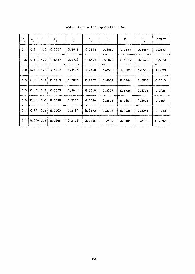
Table . IV - A for Exponential Flux

CJ0.1

0.5

0.9

0.5

0.5

0.5

0.1

0.1

C2

0.8

0.8

o.a0.95

0.95

0.95

0.95

0.975

a

1.0

1,0

1.0

0,1

0.5

1.0

0.3

0.3

F.

0.3838

0.61B7

1,4927

0.6193

0.3683

0,2640

0.2ÜÜ3

0.2266

F!

0.3613

0.5736

1.4133

0.7693

0.3616

0.2560

0.3134

0.2422

F2

0,3528

0.5492

1,3158

0,7152

0,3689

0,2595

0.3172

0.2446

F3

0,3581

0,5627

1,3506

0,6969

0.3727

0,2801

0.3236

0.2489

F,

0,3585

0,5635

1,3531

0,6985

0.3720

0,2601

0.3239

0,2491

F5

0.3587

0,5037

1,3538

0.7000

0.3726

0,2601

0.3241

0.2492

EXACT

0.3587

0,563B

1.3539

0,7010

Q.3726

0,2601

Ù.3240

0.2492

105

THE INTEGRAL TRANSFORM METHOD, THE DIRECT METHOD ANDTHE TENSORIAL METHOD IN NEUTRON TRANSPORT THEORY

The integral transform method

The integral transform method as developped by the Bologna Groupgoes back to 1968 t BOFFI and MOLINARI, 1968^, and since thenhas received application to various physical situations. For a,nexhaustive bibliography of the period 1968-73 the reader shouldrefer to ["BOFFI, 1974 J . Some of the most recent applicationsare illustrated in the next Chapter IV, whereas other applications,like, for instances, the ones related to the anisotropy of thescattering and fission, to the multigroup formulation and to otherfields allied to the neutron transport will not be covered here.We confine ourselves to the case of isotropic scattering and fis-sion and to a one speed-model. For a homogeneous body of totalcross section f dZ5*2 -v-2 and occupying a volume VcR the totalflux <p (x) is governed by the linear integral equation

Ç.

where

being pv uO the characteristic function of the volume V of thebody. Analogous expression holds for the inhomogeneous sourceterm S (x) .If

K 05)=- where B is a vector parameter - denotes the three-dimensionalFourier transform of a function h(x) measurable on Ra, , then forthe spatial Fourier transform of Eg. (1) we get

where

1a

4 a

andvs&^\ _ ^T^V-s-^ C-/R\

4b

106

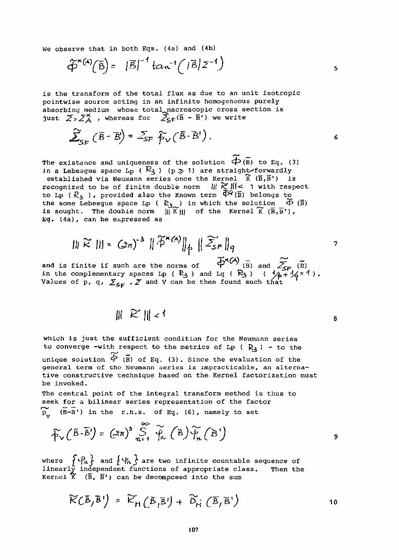
We observe that in both Eqs. (4a) and (4b)

is the transform of the total flux as due to an unit isotropicpointwise source acting in an infinite homogeneous purelyabsorbing medium whose total^macroscopic cross section isjust J^fijf^ , whereas for 5p(B - B1) we write

The existence and uniqueness of the solution Cp(B) to Eq. (3)in a Lebesgue space Lp ( £3 ) (p 1 ) are straightforwardlyestablished via Neumann series once the Kernel K (B,B') is

recognized to be of finite double norm III £f /ll< 1 with respectto Lp (^^ ), provided also the Known term <P {B) belongs tothe some Lebesgue space Lp ( ß^ ) in which the solution q5 (B)is sought. The double norm j|j K~||| of the Kernel 3c (B,B'),Eq. (4a), can be expressed as

III K III * &*)-*and is finite if such are the norms of <¥ " / (B) and 2"SF (B)in the complementary spaces Lp ( £3 ) and Lq ( Rj ) ( 4,-f -^ ) .Values of p, q, £Sf- / and V can be then found such that

which is just the sufficient condition for the Neumann seriesto converge -with respect to the metrics of Lp ( ßa ) - to the

T* —unique solution CP (B) of Eq. (3) . Since the evaluation of thegeneral term of the Neumann series is impracticable, an alterna-tive constructive technique based on the- Kernel factorization mustbe invoked.The central point of the integral transform method is thus toseek for a bilinear series representation of the factor<-sx — —p (B-B1) in the r.h.s. of Eq. (6), namely to set

where I cPn._f anc iÂ-J" are two infinite countable sequence oflinearly independent functions of appropriate class. Then theKernel K (B, B ' ) can be decomposed into the sum

10

107

where rt

is a Kernel of finite rank, and

is a Kernel whose double norm can be made as small as desiredas N is taken sufficiently high. _ _By approximating the given Kernel K (B, B'), Eq. (4a) , with theKernel "K" (B, B' ), Eg. (11a) the solution of Eq. (3) becomes matterNof a simple application of the theory of linear integral equationswith Kernels of finite rank. Tne solution to Eq. (3) - associatedto a prescribed N - will be of the form

the N coefficients t ". , IF , .... , Ç being in turn solutions— 1 o 2 -J Nto the system of the N linear algebraic equations

H ^£- S % j= = b^ ^=^^> Mj^n- 7>i.=-{ ivm. ^ ^ ; <•- ' ' S 13

r%x r *where the matrix elements Ct-fi^ and the Known terms b are given by

and

• I 14brespectively. ~ _The greater is N, the more accurate is the solution ^ (B) given byEq. (12), which in the limit of N — *oo will of course reproduce theexact solution $ (B) of Eq. (3) . Tne formal inversion withrespect to B of both sides of Eq. (12) yields finally the totalflux c|> (x) , solution of Eq. (1) , in tne form

as follows by tne convolution theorem of Fourier transforms

108

When the source S (x) is removed, that is, all b = O, then thecondition o± solvability of tne homogeneous system, Eq. (13), is

which constitutes an eigenvalue problem.As an example the theory is now concisely applied to a parallelepi.ped of dimension 2In this case

TT ./x. )-i?./o)_-4,T(along the x. - axis (i = 1,2,3) .

with

ö -K-r

is,

According to tne Geyenbauer-Clebsch formula

L7Twith

, a, S

Then, in Eq. (11a)

and

and Eq. (11a) itself becomes

With

i rlS

109

the approximation of order N, Eq. 112), is

The Fourier inverse of the needed functions are

Then, with the position ^

the approximate solution in the original domain is

The main problem is to evaluate the matrix element

of the system of Eqs. (13) from which the coefficientsmust be extracted. This can be done analytically in the monodimen-sional cases (plane, spherical and cylindrical) . Numerical resultsfor the main physical quantities and for the monodimensional planeand spherical cases have been extensively reported. For the two-andthree-dimensional cases different approximate schemes can be devised(see also Section 4) .

The direct method

By direct method we mean the method by which the concepts and theconstructive techniques -which in the previous subsection have ûeenadopted to solve Eq. (3) for the trails-form 4> (B) of the total fluxcp (x) as defined by the original Eq. (1) - are now directly appliedto Eq. (1) itself with Rj replaced by the domain D occupied by

110

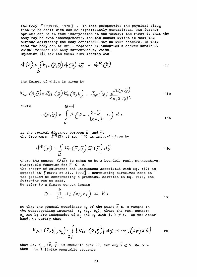
the body ^PREMUDA, 1970J . In this perspective the physical situation to be dealt with can be significantly generalized. Two furtheroptions can be in fact incorporated in the theory: the first is that thebody may be even inhomogeneous , and the second option is that thesurface delimiting the body considered may be even concave. In thiscasa the body can be still regarded as occupying a convex domain D,Which includes the body surrounded by voids.Equation (1) for tho total flux becomes now

D

the Kernel of which is given by

18a

where

is the optical distance berween x and y.The free term q>^ (x) of Eq. (17) is instead given by

- SD

where the source Q (x) is taken to be a bounded, real, monnegative,measurable function for x <£ D.The theory of existence and uniqueness associated with Eq. (17) is•exposed in j^BOFFI et al., 1973J . Restricting ourselves here tothe problem of constructing a practical solution to Eq. (17), thefollowing can be said.We refer to a finite convex domain

D= TT Xt

so that the general coordinatethe corresponding interval lâ^ and b^ are independet of x-hand, we verify that

x^ of the point x Ê D ranges in(a^ , b^) , where the real numbersand x, with j, 1 j£ i. On the other

-*-«.20

that is, K (x, y) is summable overthen the infinite countable sequence

for any x É D. We form

111

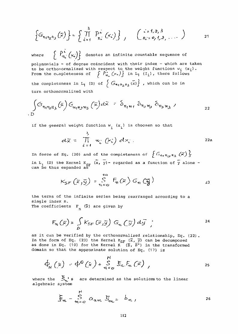
21

f Sl'(x*-)rwhere ' x*- denotes an infinite countable sequence ofpolynomials - of degree coincident with their index - which are takento be orthonorraalized with respect to the weight functions w^ (x ) .From the completeness of $ P^ („*<•)} i-n L1 (Ij.) / there follows

the completeness in L,, (D) of ) (S-n<T> ^ (x) £ , which can be inturn orthonormalized with

22D

if the general weight function w. (x.) is choosen so that

-x - TT >*•/ 0*1) ^xt - 22ai -

In force of Eg. (20) and of the completeness of T Yiîn L (D) the Kernel K (x, y) - regarded as a function of y alone -

I OJ?can be thus expanded as

the terms of the infinite series being rearranged according to asingle index n.The coefficients F (x) are given byn

S> ' '

as it can be verified by the orthonormalized relationship, Eq. (22) .In the form of Eq. (23) the Kernel KSF (x, y) can be decomposedas done in Eq. (10) for the Kernel K (B, B1) in the transformeddomain so that the approximate solution of Eq. (17) is

rftl-C3 ^ /

where the ~>^ s are determined as the solutions to the linearalgebraic system

H>- Q >~ Li= _ _^> <2 Ç _ t> . 26-ifv tM-s~> "ti"r<\. ^-'rtvi — *n. t

112

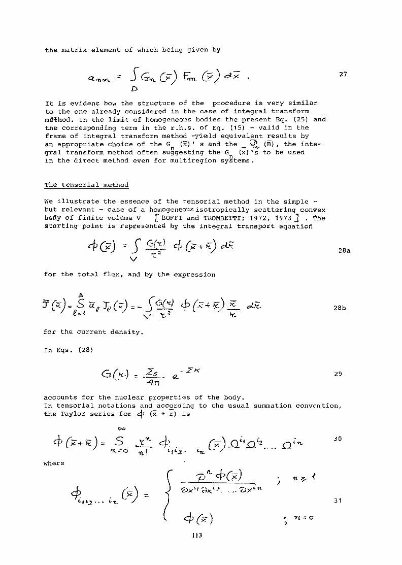
the matrix element of which being given by

It is evident how the structure of the procedure is very similarto the one already considered in the case of integral transformmethod. In the limit of homogeneous bodies the present Eq. (25) andthe corresponding term in the r.h.s. of Eq. (15) - valid in theframe of integral transform method -yield equivalent results byan appropriate choice of the G (x)' s and the _ v^ (B), the inte-gral transform method often suggesting the G (x)'s to be usedin the direct method even for multiregion systems.

The tensorial method

We illustrate the essence of the tensorial method in the simple -but relevant - case of a homogeneous isotropically scattering convexbody of finite volume V £ BOFFI and TROMBETTI; 1972, 1973 J . thestorting point is ifepresuhted by the integral transport equation

0 '- S 28aV ^

for the total flux, and by the expression

28b. •> ^ 'Vfor the current density.

In Eqs. (28)

accounts for the nuclear properties of the body.In tensor ial notations and according to the usual summation convention,the Taylor series for tfy (x + r) is

= Soo

where

' Tfl- O" f >

113

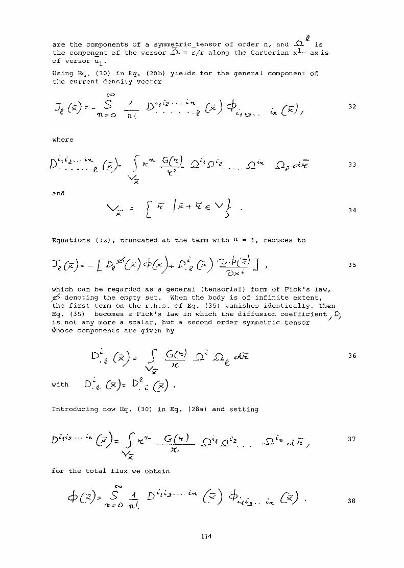
are the components of a symmetric_tensor of order n, and JÜ isthe component of the versor -O- = r/r along the Carterian x-*-- ax isof versor u-, .Using Eq. (30) in Eg. (2&b) yields for the general component ofthe current density vector

. .n > • •

where

XCxand

' x -t- »? e v 34

Eguations (2>j.) , truncated at the term with n = 1 , reduces to

"T f— \ - Y F) f~~ d>/'~"~ l OL f~~ \ f^*J "~&( ' ~(

which can be regarded as a general (tensorial) form of Pick's law,^> denoting the empty set. When the body is of infinite extent,the first term on the r.h.s. of Eg. (35) vanishes identically. ThenEg. (35) becomes a Pick's law in which the diffusion coefficient Dis not any more a scalar, but a second order symmetric tensorwhose components are given by

36v-x

with

Introducing now Eg. (30) in Eg. (28a) and setting

37

for the total flux we obtain

114

If the homogeneous medium is infinite, the usual diffusion equation

V

'x-K 2"a CP f^) Ô 394 (

is extrjicted from Eq. (38) once the series, Eq. (38), is restrictedat the term with n = 2. When the medium is not infinite and forthe same truncation, Eq. (38) would yield

40«ox '-

that can be regarded as a generalized (tensorial) diffusion equation,and has constituted an excellent basis for the development of atensorial diffusion theory.

REFERENCES

BOFFI, V., MOLINARI, V. (1968) : "Heterogeneous Methods in NeutronTransport Theory"C.N.E.N. Report - RT/FI (68) 30 - Rome

BOFFI, V. (1974) : Fisica del Reattore Nucleare Vol. I, Part 2 -Patron, Bologna

BOFFI, V., PREMUDA, F., SPIGA, G. (1973) :Journal of Mathematical Physics, 14, 346

BOFFI, V., TROMBETTI, T. (1972): Meccanica, 1_, 131

BOFFI, V., TROMBETTI, T. (1973): Nuclear Science and Engineering,_50, 200

PREMUDA, F. (1970): "Solutions for the Integral Neutron TransportEquation by Direct Decomposition of its Kernel"C.N.E.N. Report - RT/FI (70) 27 - Rome.

115

THREE-DIMENSIONAL INTEGRAL NEUTRON TRANSPORT VIAKERNEL FACTORIZATION

According to specialists in nuclear design codes, accuratebenchmarks for even idealized three-dimensional problems inneutronics could be surely useful in testing more flexible andless accurate codes. We need sometimes, in addition, accurately calculated global transport -quantities like the neutronescape probabilities from different part of the surface

£CICCON1, 197 6-77 3 of the physical system under consideration,or the ratio of the maximum to the average critical flux. Thesequantities can be used to determine equivalent diffusion para-meters like extrapolated end points, bucklings and diffusioncoefficient £PISTOCCHI, 1976-7?].Since in fast reactors scattering anisotropy plays an importantrole for core calculations too, in view of a future extensionto a multigroup treatment we started from the anisotropic mono-energetic neutron transport formulation given, for a homogeneousfinite body, by the third form of the Boltzmann equationC WEINBERG and WÏGNER, 1958]

^ / 1ao

where

{TT £ 5.)

is the distance of r from the boundary in thedirection -This line integral equation can be easily transformed, accordingto £ WILLIAMS, 1971J , into the volume integral equation

L +l

V

~_-,i2 'e-with

cj/Yrc) -' 4- -tV^/^)~Q, {. / ^ T^ / /

2bxy rc----| J- C - " "I"7"

Once the angular flux is expanded in spherical harmonics accordingto

oo 4 Qi>L

116

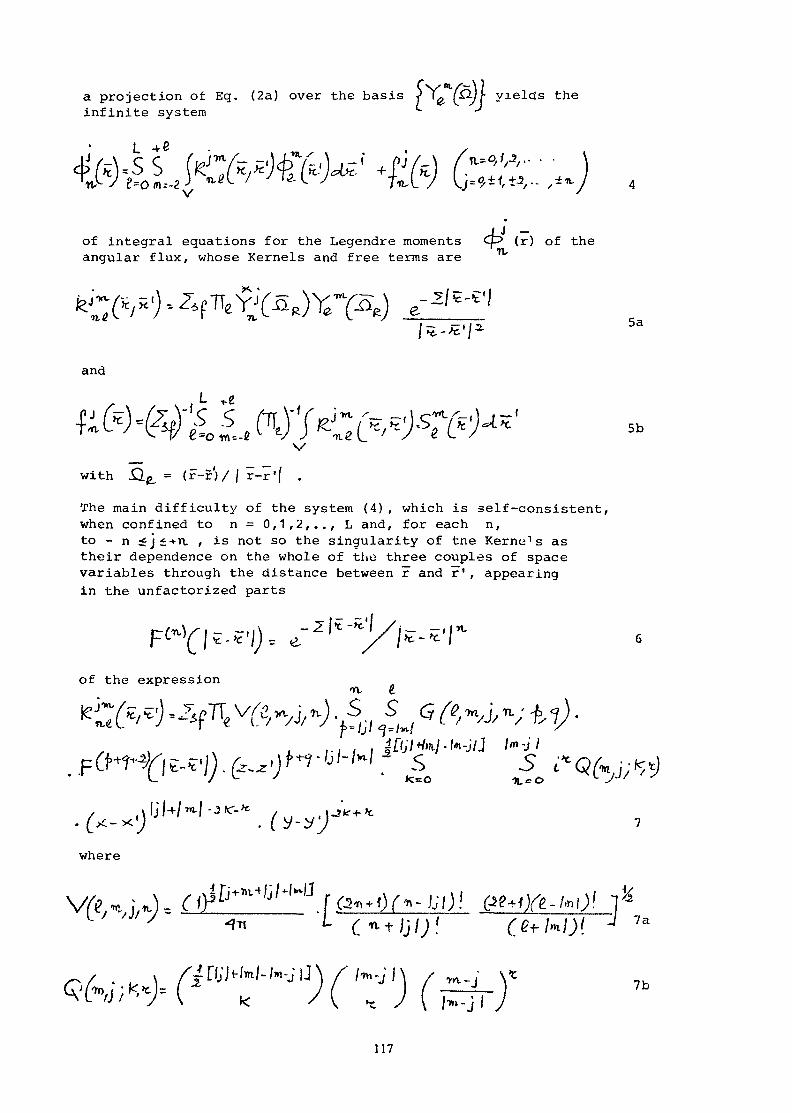
Cvm-/^\ la projection of Eq. (2a) over the basis s T^ f /f yields the• - - - < - - = > * • - înfinite system

j J -of integral equations for the Legendre moments cp (r) of theangular flux, whose Kernels and free terms are

5a

and

s/with H^ = (£-r)/jr-r'f

The main difficulty of the system (4) , which is self -consistent,when confined to n =0,1, 2,.., L and, for each n,to - n iji+rt , is not so the singularity of tne Kerne "'s astheir dependence on the whole of the three couples of spacevariables through the distance between r and r ' , appearingin the unfactorized parts

of the expression

v5 ik=o -)L = C>

where

7a

7b

117

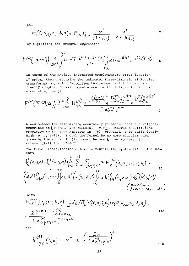
and

= P „ P, fr! <7-'->f M O. /By exploiting the integral expression

F lOo

in terms of the m-times integrated complementary error functionim erfex, then performing the indicated three-dimensional Fouriertransformation, which factorizes the u-dependent integrand andfinally adopting Gaussian quadrature for the integration in theu variable, we get

A new method for determining accurately gaussian nodes and weights,described in QPREMUDA and ZUCCHINI, 1979J, ensures a sufficientprecision to the approximation in (9), provided s be sufficientlyhigh (e.g., s=16) . Though the Kernel be no more singular -./hengiven by the r.h.s. in (9), nevertheless fc goes to very highvalues ( ;£> 1 ) for f'—^ r.The Kernel factorization allows to rewrite the system (4) in theform L +e

S S! o <M.:«£

"" ' ' 10

- C

with

t «VJ l) •ft«?« jj C* 11 a

and

118

The system (10) can be then solved via different methods, inparticular by space spherical harmonics expansion ]T BASSINI et al.,1979H[ and by tensorial diffusion nodal-modal approach (for thistreatment with Isotropie scattering see ELAND INI et al., 1979 l ).Along the first approach, the Fourier coefficients in the expan-sion

with

JFconstitute the vector solution of an algebraic system obtainedby projecting the integral equations of (10) over the basis used inthe series expansion (12). The general element of the matrix in theabove algebraic system can be expressed, according to the Kernelsfactorization, as a finite sum of products of three "one-dimensio-nal" matrix elements of the form t.

which are double integrals analytically evaluated by techniquessimilar to those already adopted in Fourier transform method forslab geometry £BOFFI and MOL IN AR 1, 1968 J £CUPINI et al., 1969^For any other detail about the calculational algorithm developedand then translated into a program, tor isötropic scattering,the reader is referred to t BASSINI et al., 1979J and[[BASSINI et al., 1977J . Tables and diagrams for subcritical fluxand for critical eingenfunction and eigenvalue, which are enclosed,should be self-explaining. The accuracy, which is very high fora 370/168 IBM computer, could be probably improved by refiningthe numerical techniques adopted.

As far fas the tensorial diffusion approach applied to the system(10), we can observe that the general coefficient ß^ ^ £x/y )of a derivative in the case of isotropic scattering is -oven simplerthan the matrix element in the previous method, since it can beexpressed as a sum of products of single integrals of the form

*/ 14

-oi.

which can be easily expressed in terms of small incomplete gammafunctions. Of course, in (14), t= X or t= y or t= z . The fulfillement of the infinite order tensorial differential equation

119

1\- 7V nrv

X-U 15

t>y the modal expansion

H h HS r* C »- ^ kr» tci5 S £^^ x \y '-e » 16

3 3in (N+1) nodes in thé positive octant yields the (N+1) homoge-neous equations allowing to determine the coefficients in Eq.(16)and the A eigenvalue. The translation of the related analyticalalgorithms fLANDINI et al., 1979 K into a FORTRAN IV program,now at an advanced stage, should attain a remarkable reductionin computing time without any loss in accuracy with respect tothe preceding approach. An interesting problem solved in£ LANDINI et al., 1979Ü regards the choice of the position ofthe nodes. For this problem and any other detail the readeris referred to f LAND I NI et al., 1979J .

B I B L I O G R A P H Y

1) L. CICCONI - "Calcolo délie probabilitä di fuga per neutronida sistemi tridimensionali in teoria del tra-sporto".Thesis for the Degree of "Dottore" in NuclearEngineering, Faculty of Engineering, Universityof Bologna, Academic Year 1976-77.

2) G. PISTOCC.'II - "Modello intermedio tra diffusione classicae trasporto: calcolo dei nuovi parametri diffu-sivi in mezzi tridimensionali finiti" .Thesis for the Degree of "Dottore" in NuclearEngineering, Faculty of Engineering, Universityof Bologna, Academic Year 1976-77.

3) A.M. WEIMBERG, E.P. WIGNER - "The Physical Theory of NeutronChain Reactors"The University of Chicago Press, 1958

4) M.M.R. WILLIAMS - "Mathematical Methods in Particle TransportTheory"Butterworths, London, 1971.

5) F. PREMUDA, A. ZUCCHINI - "A Program Computing GaussianWeights and Nodes from the Weight Function MomentsVia Orthogonalization"CNEN Report - RT/FIMA (79) 2, Rome, 1979.

120

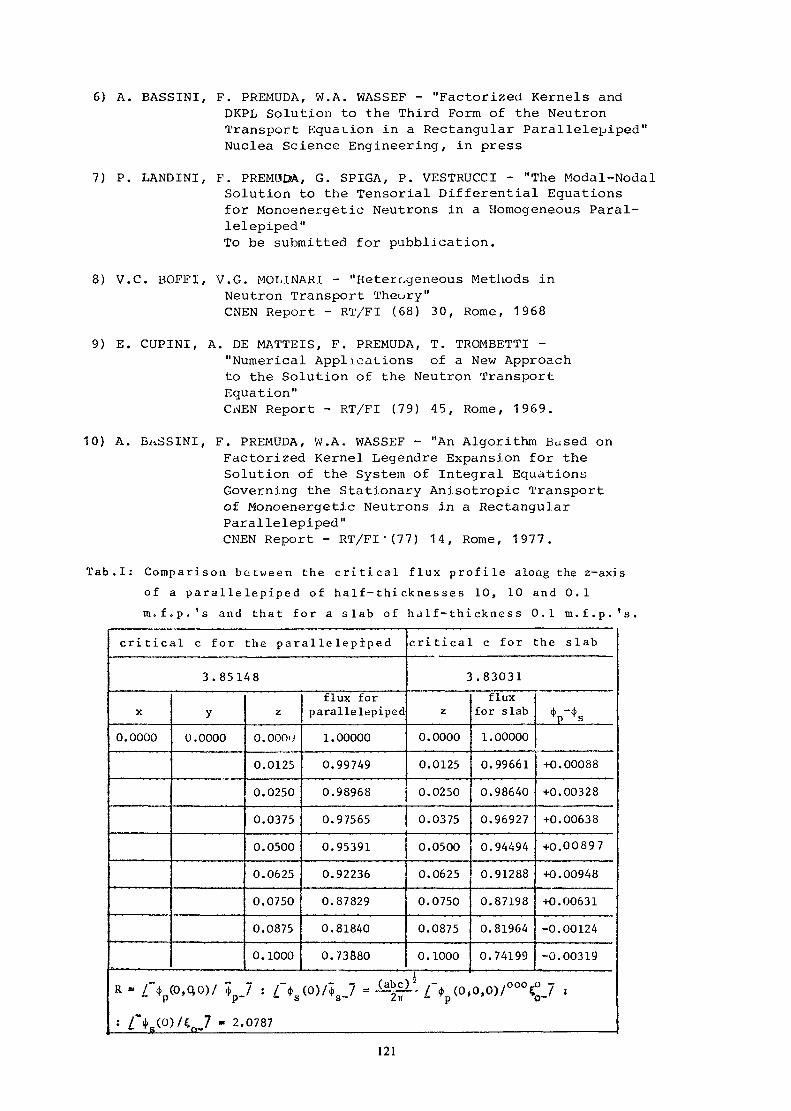
6) A. BASSINI, F. PREMUDA, W.A. WASSEF - "Factorized Kernels andDKPL Solution to the Third Form of the NeutronTransport Equation in a Rectangular Parallelepiped"Nuclea Science Engineering, in press

7) P. LANDINI, F. PREMUDA, G. SPIGA, P. VESTRUCCI - "The Modal-NodalSolution to the Tensorial Differential Equationsfor Monoenergetic Neutrons in a Homogeneous Paral-lelepiped"To be submitted for pubblication.

8) V.C. BOFFI, V.G. MOLINARI - "Heterogeneous Methods inNeutron Transport Theory"CNEN Report - RT/FI (68) 30, Rome, 1968

9) E. CUPINI, A. DE MATTEIS, F. PREMUDA, T. TROMBETTI -"Numerical Applications of a New Approachto the Solution of the Neutron TransportEquation"CNEN Report - RT/FI (79) 45, Rome, 1969.

10) A. BîSSINI, F. PREMUDA, W.A. WASSEF - "An Algorithm Bused onFactorized Kernel Legendre Expansion for theSolution of the System of Integral EquationsGoverning the Stationary Anisotropie Transportof Monoenergetic Neutrons in a RectangularParallelepiped"CNEN Report - RT/FI'(77) 14, Rome, 1977.

Tab.I : Comparison between the critical flux profile along the z-axisof a parallelepiped of half-thicknesses 10, 10 and 0.1m.f.p.'s and that for a slab of ha If-thickness 0.1 m.f.p. 's.

cr i t ica l c for the p a r a l l e l e p i p e d

3.85148

X

0.0000

y0.0000

z

O.OOOiJ

0.0125

0.0250

0.0375

0.0500

0.0625

0.0750

0.0875

0. 1000

flux forparallelepiped

1.00000

0.99749

0.98968

0.97565

0.95391

0.92236

0.87829

0.81840

0.73880

cr i t ica l c for the s lab

3.83031

z

0.0000

0.0125

0.0250

0.0375

0.0500

0.0625

0.0750

0.0875

0.1000

R - /"yo, o,o)/ ?p_7 ; r*s<o)/+8_7 - -^g^ /'yo,

: AR(0)/enJ - 2.0787

fluxfor slab

1.00000

0.99661

0.98640

0.96927

0.94494

0.91288

0.87198

0.81964

0.74199

(j, -4,p s

+0.00088

+0.00328

+0.00638

+0.00897

+0.00948

+0.00631

-0.00124

-0.00319

0,0)/OOÛÇ°_7 ,

121

(O

Tab. IICritical flux p rof i les for the pa r a l l e l ep iped of h a l f - t h i c k n e s s e s 10, 10and 0.1 m. f.p » 's.

X

0.0000

il

ii

0.0000

1.2500

2.5000

3.7500

S. 0000

6.2500

7.5000

8.7500

10.0000.

y0.0000

———

0.0000

z

0.0000

0.0125

0.0250

0.0375

0.0500

0.0625

0.0750

0.0875

0.1000

0.0000

t ^

i: (

total ;, flux

1.00000

0.99749» —————— r0.98968

.

0.97565

'0'. 95 3 9-1

0.92236

0.87829 i

0.81840

0.73880

1.00000

0.98585

0.94331

'0.87211

0.77179

0.64171

Oi.lSlO?

0.28885

0.063S82

iX

10.0000

tr

»•i

0.0000

1.2500

2.5000

3.7500

5.0000

6 . 2500

7.5000

8.7500

10.0000

y0.0000

0.0000

z

0.0000

0.0125

0.0250

0.0375

0.0500

0.0625

0.0750

0.0875

0.1000

0.1000

tocalflux

0.063882

0.065730

0.063256

0.062400

0.061066

0.059119

0.056384... .. ... ,._ ... ........0.052649

0.047660—— — . ——

0.73880

0.72832

0.69683

0.64414

0.56994

0.47380

0.35518

0.21340

0.047660 -i

xx

10.00001111

0.0000

1.2500

j 2.5000

3.7500

5.0000l ———————

6.2500

7.5000

8.7500

j 10.0000

y10.0000

10.0000

z

0.0000

0.0125

0.0250

0.0575

0.0500

0.0625• . _

0.0750

0.0875

0.1000

0.1000

totalflux

0.0045953

0.004585^

0.0045527

0.0044942

0.0044023

0.0042674

0.0040766

0.0038146

0.0034631

0.047660

0.046976

0.044920

0.041491• ———————0.036682

0.030486

0.022R93

0.013890

0.0034631

Tab. Ill: Critical c for a parallelepiped of ha If -thicknesses10,1 and 0.5 m.f.p.'s versus N and G .

\G\P

N \

2

4

6

10

1.888622

1.888566

1.888516

11

1.888791

1.888743

1.888702

12

1.888863

1.888817

1.888785

13

1.888858

1.388810

1.888786

14

1.888825

1.888774

1.888755

15

1.888797

1.888745

1.888728

!

16

11.888785

1.888732

1.888717

Tab. IV - Critical c for two parallelepipeds of optical half--thicknesses 0.5, 1, 10 and 0.5, I,00 for diiferentN (and G = 16).P

N

2

4

6

8

10

12

M

c for (0.5, 1, 10)

1.888785

1.888732

1.888717

_

c for (0.5, 1,~)

1.883723

1.883691!

1.883675

1.883668

1.883666

1.88366511.883664 !

123

Tab. V: Subcritical neutron flux, for an Isotropie sourceS(r, ft) = l/4ir uniformly distributed in a parallelepiped

of half-thicknesses 10, 1 and 0.5 m.f.p.'s.

X

0.0

0.0

0.00.0

0.0

0.0}...,._..0.0

10.0

y0.0

0.0

0.0

0.0

z

0.0

0. 1

0, 2

0.3\o.o ; 0.4

0.0

1.01.0

0.5

0.5

0.5

flux1.35958

1.343701.29278

1. 197031.04012 ;

0. 79918

0.42527 \

0.30709

X y0.0 | 0.0

j 0.0

0.0

0.0

0.0

0.0

10.0

10.0

0.2

0.4

0.60.8

1.0

1.0

0.0

z

0.0

0. 0

0.0

0.0

0.0

0.0

0.0—————0.5

flux

1.35958

1.346591. 30044

1. 199571.00808

0.67571

0.49795

0.56651

124

MIXED METHOD AND SPACE POLYNOMIAL APPROXIMATIONS

It is known that one of the biggest advantages of Integral TransportMethods is the direct introduction in the formalism of relevant quantitieslike scalar fluxes and other spherical harmonic components. Then theangular fluxes needed by DSN methods are useless, and the drawbacks ofthese methods (negative angular fluxes, ray effects, etc. ) are eliminated.The integral transport formalism has been therefore applied in the pastwhenever a high accuracy was required. Unfortunately two limitationsappeared in practice:

1) the usual numerical schemes involved some crude approximationslike flat sources, discretized transport kernels, etc. and inorder to mitigate them, very narrow space meshes had to bechosen HO that only reactor cells and very small criticalassemblies could be calculated by this way;

2) the scattering anisotropy could not be easily introduced in theformalism and therefore shielding calculations were outsidethe scope of applications.

As soon as 1970 we could at Würenlingen improve very much theIntegral Transport Methods with respect to these both drawbacks by usingspace polynomial approximations for 1. D cylindrical geometry in theframe of the so-called "mixed method" (LiGOU, 1970). The first resultsobtained with the SHADOK code have shown that very large multilayersysteins (whole reactors and shieldings) could in fact be analyzed withsuch improved methods (LIGUUetal , 1972). In the same time the integraltransport equation was solved for homogeneous spheres and slabs byusing various approaches, J. STEPANlKcould show that among about tendifferent method« the Legendri1 polynomial approximations, originallyproposed by CAliLVK (19G8), were, by far, the most powerful (STEPANEK,1972). Moreover MIKA (1909) and BOM (1968) could prove that theIntegral Transform Method (A.SAOKA.1968) and the Carlvik approach wereexactly the same. All these results could explain why the SIIADOK codewas faster than DSN codes although rather low degree polynomials wereincluded.

It has been therefore decided in 1972 to develop a general formalismBuitiible for the three 1 1)-geometries in which any kind of polynomialapproximation or scattering anisotropy is assumed in each zone. On theother hand the basic ideas of the mixed method have been used as muchas possible what leads to a much simpler formalism as shown below.

Space polynomial approximations have also been proposed by BOSEVSKI(1970) for cell calculations and isotropic scattering.

1. The Mix-ed M e t h o d

In order to make clearer the main features of the mixed method,let us consider the plane geometry and one energy group (the extensionto multigroup schemes is straightforward). We assume moreover somedegree of scattering anisotropy what increases the complexity of theusual integral transport formalism.

125

For an isolated system one has the following set of integral equations(STEPANEK.1972, 1974):

r 2m+l

m=0

J d x ' q (x ' ) e (x ,x ' ) f° ^ P ( l ) •" l e

(D

P (I)e-T ( x ' x < ) um u

in which T(X, x1) represents the optical thickness (between x and x1)and e is given by:

1 for x > x1

, , .e +m . .(-1) for x < x1

The emission rate q (x) is calculated from the flux and sourceLegendre components:

If the order of anisotropy is L, L integral equations should be solvedsimultaneously.

On the other hand one can write the usual differential equationsgoverning the spherical harmonics as follows:

( 2 e + i ) dx ' (2e+i ) dx ' - tx~'*e ( x ) = qe (x) (3)

where q = 0 if g > L. If the Eq. 3 is written for g = 0, 1, . ... L-1C

one obtains a set of L equations with (L+l) unknowns (cp0, cp1, . . . ,cpT ). Therefore another equation must be found; there are twopossibilities:

1. Eq. 3 is used once more by assuming that cpT , . = 0, this is theusual P, approximation.

2. One of the exact integral Eq. (1) is used (e = 0 for instance) and solvedsimultaneously with the L rigorous differential Eq. 3 (gs L-l).

The last method is called the "mixed method". The main properties ofthis method are as follows:

1. Compared to the PL method no flux component ( $ ) isneglected; therefore, the value of L \vill be fixed only bythe characteristics of the scattering kernel and not bythe flux anisotropy.

2. Compared to the pure integral methods, Eq. (1), the accuracyis the same but the number of required integral equations issmaller, 1 compared to (L + l).

Numerically, the advantages of the mixed method are quite evident andit is strange that such an approach has been neglected in most of thenumerical methods based on integral transport theory, except sometimes

126

for linear anisotropy (L = l) where the balance equation has been used(BRUN, 1971).

As a first example it is interesting to see how the Collision Probability(CP) method can be reformulated. One.usually starts from Eq. 1, thespace integral being split into layers over which the "flat source approx. "is made: q (x1) ~ q i . A double integration is then performed over

x1 in the mesh i and over x in the mesh j. Finally one has to solve:

with the transport coefficients:

f m 2m-H r. p . T du r„ . l .Ag ( j , i ) = — g — — J J dx dx1

e (x, x ' ) . J — [P£(-)

i 3

p ( I ) e - T ( x ' x l ) u l with V.= x . -x . , (5)m u J 1 1 i - l

If, on the contrary, the Eq. 3 is integrated over meshes the § (x.)

are connected to the q^ in a simpler way, but in order to close thesystem supplementary equations are needed. Setting x = x., 8=1 inEq. 1 a single integration over x' will lead to:

L J

where

, . . . l l li V. 1i

With the mixed method (Eq. 6-7), only (L+l ) matrices J x J must becalculated instead of (L+l)2 with the usual approach (Eq. 4-5). Moreoverthe probabilities P,m are much easier to compute than the coefficients

A . Finally one can show, by using Eq. 2, that the scalar fluxes |0are solutions of a I x I system of linear equations. The scatteringanibotropy terms can be completely eliminated.

For cylindrical and spherical geometries similar improvements canbe achieved what allows some degree of scattering anisotropy (L = 5 forexample). One is no longer limited to linear anisotropy ( L = l ) as itresulted in practice from the usual integral transport approachrfAKAHASHI, 1966).

The layer thickness must be still small since, the "flat source approx.has been kept and there is no improvement to expect on this side. Onecan see in the next section how this la'st drawback can be removed byusing space polynomial approximations.

127

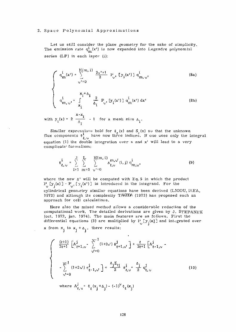
2 . S p a c e P o l y n o m i a l A p p r o x i m a t i o n s

Let us still consider the plane geometry for the sake of simplicity.The emission rate q1 (x1) is now expanded into Legendre polynomial

series (LP) in each layer (i):

•*• / i \ \ •" V ' A T-* r / i \ 1 * / n \3 (x1) = ) ——— P [y . (x ' ) ] q (8a)m _i_, .s v i m, vv ' ~ 0

Vv'= -T A~ pv- &i<*'>:i t i ( x l ) d x l (8b)xi

x-x.with y.(x) = 2 ——— - 1 for a mesh size A..

Similar expressions hold for $ (x) and Si (x) so that the unknownflux components $L have now three indices. If one uses only the integralequation (1) the double integration over x and x1 will lead to a verycomplicate'- formalism:

J L N(m, i)1 V"1 X- V** = y y y ' A^'U.W , m8, v L, L, L, £, v m,v

i=l m=0 v ' =0

where the new A' will be computed with Eq. 5 in which the productP [y.(x)] • P , [y . (x ' ) ] is introduced in the integrand. For the

cylindrical geometry similar equations have been derived (LIGOU, IAEA,1972) and although its complexity TAKEOl (1973) has proposed such anapproach for cell calculations.

Here also the mixed method allows a considerable reduction of thecomputational work. The detailed derivations are given by J. STEPANEK(oct. 1972, Jan. 1974). The main features are as follows. First thedifferential equations (3) are multiplied by P [y.(x|] and integrated over

V J

x from x. to x. + A . , there results:J 3 3

;-lu 3 v M+2v,n «3 1LAe+i,v L ( v } Vi,v' J2e+i L e+i.v L Te+i.v' J 2e+i L e-i.v

v' = 0

v-_ V

irl • _ A.E . A.- -V *L= f qL (10)

where

128

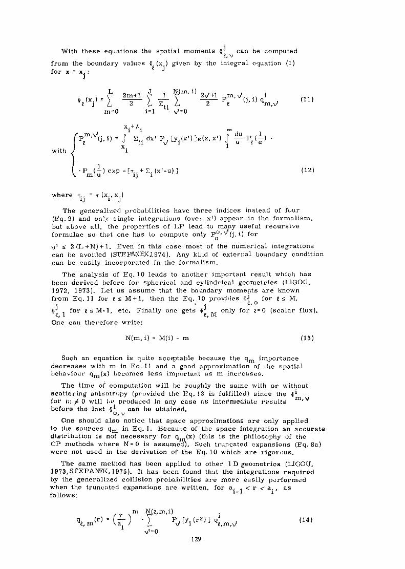
With these equations the spatial moments $ can be computed

from the boundary values $ (x.) given by the integral equation (1)for x = x. : -1.

3

2v'+l

m = 0 i=l v' = 0

oo1 , -r-, r / I \ l / I \ n Û T> / 1 \. dx' P . [ y . ( x ' ) Je (x, x1) — 1 ( — ) •

i v i i u 2 uwith

(12)

where T. . = T (x., x.)J J

The generalized probabilities have three indices instead of four(Eq. 9) and only single integrations (over x1) appear in the formalism,but above all, the properties of LP lead to many useful recursiveformulae so that one has to compute only P0> v (j, i) for

v1 £ 2 ( L + N ) + 1. Even in this case most of the numerical integrationscan be avoided (STEPANEKA974). Any kind of external boundary conditioncan be easily incorporated in the formalism.

The analysis of Eq. 10 leads to another important result which hasbeen derived before for spherical and cylindrical geometries (L1GOU,1972, 1973). Let us assume that the boundary moments are knownfrom Eq. 11 for es M + l, then the Eq. 10 provides $3 for i < M,

i . . 8 , 0f 1 for e sM-1 , etc. Finally one gets fj only for e= 0 (scalar flux).

c, A c> *•••One can therefore write:

N(m, i) = M(i) - m (13)

Such an equation is quite accq>table because the qm importancedecreases with m in Eq. 11 and a good approximation of ihe spatialbehaviour qm(x) becomes less important as m increases.

The time of computation will be roughly the same with or withoutscattering anisotropy (provided the Eq. 13 is fulfilled) since the f*fol' tu ^ 0 will U1 produced In any case as intermediate results m'Vbefore the last $* can bo obtained.o, v

One should also notice that space approximations are only appliedto the sources qm in Eq. 1. Because of the space integration an accuratedistribution is not necessary for qm(x) (this is the philosophy of theCP methods where N = 0 is assumed). Such truncated expansions (Eq. 8a)were not used in the derivation of the Eq. 10 which are rigorous.

The same method has been appliud to other l D geometries (LIGOU,1 973, STEPANEK, 1975). It has been found that the integrations requiredby the generalized collision probabilities are more easily performedwhen the truncated expansions are written, for a. - < r <r a. , asfollows: : 1

m N(K,m, i )

'I Wr2)]cWwv' = 0

129

where a. 1 and a. are respectively the inner and the outer radii of

the shell (i). The argument of the LP are now given by:

2 r2 , . . . „ , ~i /, -, ... i-1r 9 r2 -iy.(r2) = ^%- - ( I 4 , i ? ) l l-a.? withl L &. ! J l_, _ a.i i

Although the Eq. 10-11 become more complicate, many recursiveformulae can be derived so that the computation of the generalized CPremains tractable. Moreover, as for plane geometry, the mixed methodallows further improvements. The space moments for e ^ 0 can bein principle eliminated from the final equations which only involve thescalar flux moments ( $1 , ). One has therefore to solve a "compacto, o, vsystem" N . J x N . J, and its size is such that generally the Gausselimination technique can be used, then the inner iterations are complete-ly avoided and a high accuracy is achieved.

3 . N u m e r i c a l A p p l i c a t i o n s

As said before the :'irst version of the SHADOK code was completedin 1970 for cylindrical geometries with a three terms polynomialapproximation (N = 2) and a linear scattering anisotropy ( L = l ) . Multi-group calculations have shown that, even for deep penetration problems,such an approach was very powerful. Later on a more accurate version(N = 3) was extended to the spherical geometry (UDOCJ, 1972-1973) andit came out that the introduction of a fourth term in the qm expansionscould allow much thicker layers (5 to 10 m. f. p) and a now reductionof the computation time was achieved.

These codea were still restricted to PI scattering, but most reactorcalculations are usually made in the frame of such an approximation(even in PO). The second extension deals with plane geometry with norestriction on space alid scattering approximations (STEPAMiK,1972J 1974).The SHERLOCK code based en this general formalism (see the previoussect. ) has been successfully applied to many shielding problems».

More recently the limitations of the SHADOK codes have bo<»nsuppressed. In fact a new code SIIALOC'K, based on a more involvedformalism, has been ekilmt'ated (STEPANtTK,197D). Now with SllfiRLOCKfor plane geometry and Hl iALQCK for «spherical and cylindrical guoniutryall 1 D-trunsport problems carl bo solved for any scattering unisotropyand l'Or complex multilayers arrangements. For all practical situationsthe SN methods could be replaced by the proposed inu-^ral transportmethods* and the reduction of the computation time should be at lenBta factor five (in many cases more than 10) as shown below with afew L'xamples dealing with large systems.

(SHERLOCK code)

A fission neutron source is embedded in a water shield, the scatteringanisotropy is therefore important. The plane source is situated on theleft boundary of the shield which is 120 cm thick.

*A11 these codes use the same data as ANISN the mostpopular DSN code

130

Seven group calculations were performed and the codes SHERLOCK andANISN were compared (STEPANEK, 1974). In the following the approximationsare labelled by Sn/J for ANISN and N/J for SHERLOCK where J is thenumber of meshes, N the number of Legendre polynomials (in space)and Sn the number of directions. The flux variations in ti o seventh grouprepresent 7 to 8 orders of magnitude, but SHERLOCK requires only6 layers with a P3 approximation in space (the usual CP method wouldhave required 100 layers at least, without scattering alü.ôtropy). The4/6 approximation gives the same results on the right boundary (lessihan 0. 2% difference.'), Comparing the ANISN and the SILERT-OCK resultsone sees that only S^ calculations are accurate enough. Coillparing thecases 3/6 with 24/122 it comes out that for PQ scattering approximationANISN requires about 10 times more computing time than SHERLOCKand for the E, approximation about 6 times. Again SHERLOCK is moreaccurate.

On the other hand, the computation time with the mixed method doesnot increase with scattering anisotropy as it could be feared with normalintegral transport treatment (Fig. 1). In this figure the computation timefor the case N/J = 3/G calculated by SHERLOCK is compared with thecomputation times for 16/122 and 24/122 cases computed by ANISN.The relative accuracies are also quoted. In this version of SHERLOCKa dimple iterative scheme was used to calculate the flux from theintegral transport matrix. Both, from this and from a programmingpoint of view, this versioh could be improved what has been donerecently.

code)

Among the fast critical assemblies, Zl'R-3-48 is one of the largest.The composition is very similar to that of a plutonium fueled LMFBR.For an accuracy of 0. 1% on the eigenvalue one needs at leat.t S^ and40 points with ANISN and only four layers (with N = 3) with SHADOKwhich is six times faster (LKOJ, 1973). For smaller assemblies(GODIVA, TOPSY, e tc . ) the differences between ANISN and SHADOKare, of course, more pronounced (factor 20 to 50 1 ).

The central reactivity worth experiments have been analyzed fdr thisassembly, Two eigenvalue calculation« must be performed, with andwithout t i ic central sample. The A k values can ho in the range of 0. 1%for less) und ihcroforo the kpj.j. must bo i 'ulculuted wi th 5 ot1 6 figures.

This is possible with SHADOK which uses the Gauss method (or a matrixinversion).' With , \NISK this is very difficult because of the inner iterationprocedure ( 1 0 ~ » difference on the last two iterations can mean 10"4 erroron the eigenvalue). For this reason the perturbation theory has been widelyused to solve this problem with DSN codes, but sometimes this is not 'correct since the local perturbations can be large.

Shielding calculations have also been performed. For example the deeppenetration of neutrons in water has been analyzed for a point mono-energetic source. With 20 shells, 15 decades of flux variation wereobtained in one run (GANAPOL,oct, 1972). For the same acc;,acy theANISN calculations required a bootstrapping technique (several runs) anda longer time of computation. Therefore, from the point of view ofstorage, the proposed method seemt> more attractive.

Similar examples dealing with the cylindrical geometry (whole reactorand shielding calculations) have led to the same conclusions. The usualstatement: "the integral transport methods are only suitable for systemswith small optical thicknesses" is therefore quite wrong. Finally one

131

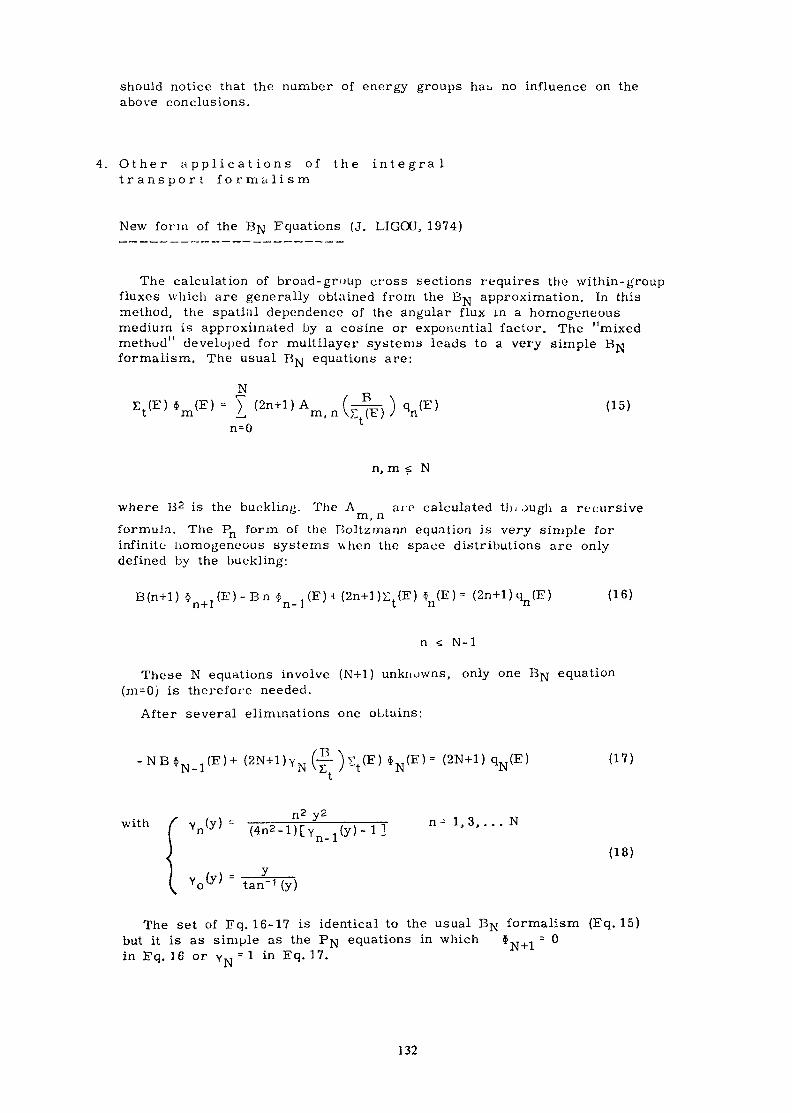
should notice that the number of energy groups ha^ no influence on theabove conclusions.

4 . O t h e r a p p l i c a t i o n s o f t h e i n t e g r a lt r a n s p o r t f o r m a l i s m

New form of the BN Equations (J. LIGCU, 1974)

The calculation of broad-group cross sections requires the within-groupfluxes which are generally obtained from the BJJ approximation. In thismethod, the spatial dependence of the angular flux in a homogeneousmedium is approximated by a cosine or exponential factor. The "mixedmethod" developed for multilayer systems leads to a very simpleformalism. The usual BJVJ equations are:

N(2n+ l )A ( y ' f E M ) Q (E) (15)

n=0 l

n, m ^ N

where B2 is the buckling. The A arc» calculated th rough a recursiveformula. The Pn form of the P.oltzmann equation is very simple forinfinite Homogeneous systems u hen the space distributions are onlydefined by the buckling:

B(n+l) $ , ( E ) - B n * . (EH (2n+l )£. (E) * (E) = (2n+l) a (E)n+J n- i t n "(16)

n <. N-l

These N equations involve (N+l ) unknowns, only one Bj^ equation(m=0) is therefore needed.

After several eliminations one obtains;

- N B $ N _ 1 ( E ) + ( 2 N + l ) Y N ( - | - ) ï t ( E ) $ N ( E ) = (2N+1) q^ÇE) (17)

n= 1,3,... N

(18)

Y (y) = — i7-\Yo^' tan"1 (y)

The set of Eq. 16-17 is identical to the usual B^j formalism (Eq. 15)but it is as simple as the P^ equations in which $Ta+i = °in Eq. 16 or YN

= 1 in E<3- 1?-

132

The usual approach for computing the diffusion coefficients fails fortwo reasons: (a) the voided region is located at the cell boundary, and(b) the pitch is such that two-dimensional infinite gapt. extend throughthe reactor. For an infinite lattice, the diffusion coefficient will diverge,which means that, in principle, the diffusion theory is no longer valid.This fact has been more or less forgotten because moat theories assumecylindrical cells and therefore remove this difficulty artificially. Introducingthe real height of the reactor tu the beginning, a new theory of thestreaming, which generalizes the usual approach has been developed;it appeared in the diffusion coefficient a buckling dependent term whichdiverges slowly for an infinite lattice. Fortunately, this term is smallfor usual reactor Hizes, and one may, therefore, continue to usediffusion theory for practical calculations. Let us consider an hexagonallattice with the pitch 0, then tho problem arisen only when

-r— s > 2a where 2a is the fuel pin diameter.I .—If we set e = —z—s-2a (the thickness of the two-dimensional infinite

gaps) we obtain for the diffusion coefficient:

where B2 is the axial buckling.

For tight lattices (e < 0) one has to set e = 0 and the above equationprovides the usual diffusion coefficient Do (which depends of course onthe geometry). For large pitches ( e > 0 ) a slightly buckling dependentterm appears in the formalism but only a rough value of this bucklingis needed before reactor calculations can be undertaken. Finally a isa dimensionless quantity which is obtained through numerical calculations(in a large domain we have found o. 0.077).

2D Geometries

The extension of the mixed method to complex systems in 2D geometryis extremely complicate. It is usually thought that is better to restrictsuch an approach to the computation of the fluxes inside 2 D coarsemeshes by making some assumptions on the incoming angular fluxes. Inother words the integral transport methods can provide the transfermatrices for each mesh and afterwards the connections between thesemeshes are made more or less in the same way as it appears in DSNcodes. For this reason these methods (surface currents, QPj\r, etc. )are discussed in the Chapter IV.

R E F E R E N C E S

ASA OKA T. J.of Nucl. Energy, 2£, 99 (1968)

BOFFI V./MOI.JNARI, V (1968): "Heterogeneous Methods in NeutronTransport Theory" C.N.E.N. Report -R1/FI (68) 30 - Rome.

133

BRUN A . M . and KAVENOKY A. "Acceleration Technique for the Solutionof Boltzmann Integral Equation" ANS Nat. Topi. Meeting,Idaho Falls, March 29-31 (1971)

CARLVIK I., Monoenergetic critical parameters and decay constantsfor small homogeneous spheres and thin homogeneous slabs,Nucl. Sei. Eng. 3j_ (1968) 295-303 et AE-273 (1967)

GANAPOL B.D., HERltNRERGER V., and PARATTF J. M."Comparison of New Transport Calculational Methods for ReactorSi leid Design", Proceedings of the Fourth Internatiornl Conferenceon Reactor Shielding, Paris, October 9-13, 1972

KOEHJLER P. anJ LIGOU J. Axial Neutron Streaming in Gas-CooledFast Reactors, Nucl. Sei. Eng, 54_, 357 (1974)

LIGOU J., THOMI P.A. - Equation Intégrale de Transport en géométriecylindrique a une dimension - Approx. polynomiale et diifusionanisotrope linéaire - EIR-Bericht Nr. 188/189 (Dec. 1970)

LIGOU J. , STEPANEK J. , THOMI P.A. - Forme Intégrale del'Equation du Transport - Approx. polynomiales et diffusionanisotrope - IAEA Hi'rtiinar on Numerical lieactor Calculations(SM-154/25), Vienna .fan. 1972 (Seo also EIR-iîoi'ioht Nr. 225Sept. 1972)

LIGOU J. - Improved Integral Transport Theory by Means of SpacePolynomial Approximations, Nucl. Sei. and Eng. 50_ (1973) 135-146

LIGOU J. , STEPANFK J. - A New Form of the BN Transport Equations,Nucl. Sei. Eng. 53 (1974)

STEPANEK J. - A Comparison of the Space Legendre PolynomialsApproach wi th other Methods used for the Solution of the IntegralTransport Equation - EIR-Bericht Nr. 231 (Dec. 1972)

STEPANEK J. , LIGOU J. - A Solution of the Coupled Integral andDifferential Form of the Transport Equation using a LegendrePolynomials Source Density Approximation in Angle and Spacefor Slab Geometry - 4th International Conference on ReactorShielding, Paris, Oct. 1972 (See also EIR-Bericht JMr. °48,Jan. 1974)

STEPANEK. J., LIGOU J. , 3V1 .TPFK C. - The "Mixed" Method, aSolution of the Transport Fquation in Cylindrical GeometryMaking Use of Both its Integral and Differential Forms inHigh PN Approximation - EIR-Bericht Nr. 271 (Jan. 1975)

TAKAHASHI H. , The generali'/ed first flight collision probability inthe cylindricalized lattice system, Nucl. Sei. En^ng 24(11-66) 60-71

TAKEDA T. - Integral Transport Theory of Neutron Behaviour mHeterogeneous Lattice Cells. Dept. of Nucl. Eng. - Ofa.»kaUniversity (1973)

134

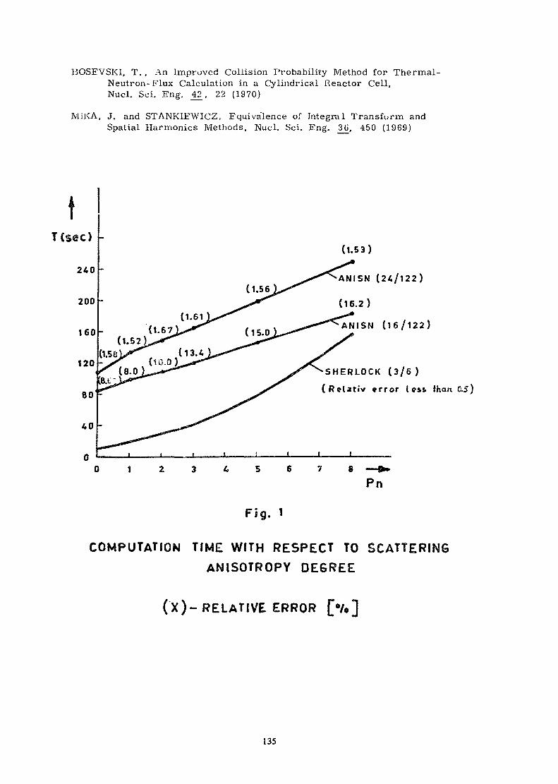
BOSEVSKI, T. , An Improved Collision Probability Method for Thermal-Neutron-Flux Calculation in a Cylindrical Reactor Cell,Nucl. Sei. Eng. 42, 22 (1970)

MiKA, J. and STANKIEWICZ, Equivalence of Integral Transform andSpatial Harmonics Methods, Nucl. Sei. Eng. 3G, 450 (1969)

Fig. 1

(1.53)**ANISN (24 /122)

(16.2)^*ANISN (16/122)

SHERLOCK ( 3 / 6 )

(Relat iv error less, than 0.5)

i____i

Pn

COMPUTATION TIME WITH RESPECT TO SCATTERINGANISOTROPY DEGREE

(X)- RELATIVE ERROR [«/.]

135

POINTWISE REPRESENTATION

l . IntroductionAccurate numerical transport theory approaches (as higher

order Sn, P , C and also Monte Carlo) may become impracticalfor repeated calculations in lattice cell burnup studies, dueto large computing time. On the other hand, the diffusion the-ory methods cannot be applied, due to strong absorbing propertiesand relatively small size (compared to the mean frcs path) of thelattice cell components. An effective approach to override thesedifficulties in burnup calculations could be the use of the col-lision probability methods based on integral transport theory(Pop-Jordanov,1974) .

The cell under investigation may be devided into K zones(each with spatially constant cross sections) . The integral tran-spoi't equation then becomes:

v £,E>= £ f dVT(r'*riE) [sk<£?E> + T'k

Where the indices i and k denote individual zones related tö rand r_" respectively.

ïf one assumes that the flux and the source within each ofthe tones are spatially constant, then *v^£.*' E*)* (E') andSk(r_*, E) « 3j(E) . With this assumption the space averagingyiealds:

K*i

The factor multiplying the square brackets is the transportcoefficient Tj,^, which can be simply expressed through the col-lision probability Pj -

Thus, by the collision probability method, in the flatflux approximation, the space-and -energy dependent integraltransport equations (1) are reduced to merely energy dependentones (2) . The obtained system of pquations (2) can be and iseffectively used for calculating the thermal, resonance and fastneutron flux and relevant parameters in lattice cells.

The energy dependence niciy be treated by standard multi-group technique, which, in face, is an analogue in energy spaceto multizone technique.

The typical example of the multizone-multigroup integral tran-sport theory approach is the THERMOS method (Honeck, 1960) . Aversion of THERMOS has been used at the Boris KidriC Instituteas well (Bosevski et al. 1967, Matauâek et al. 1978).

136

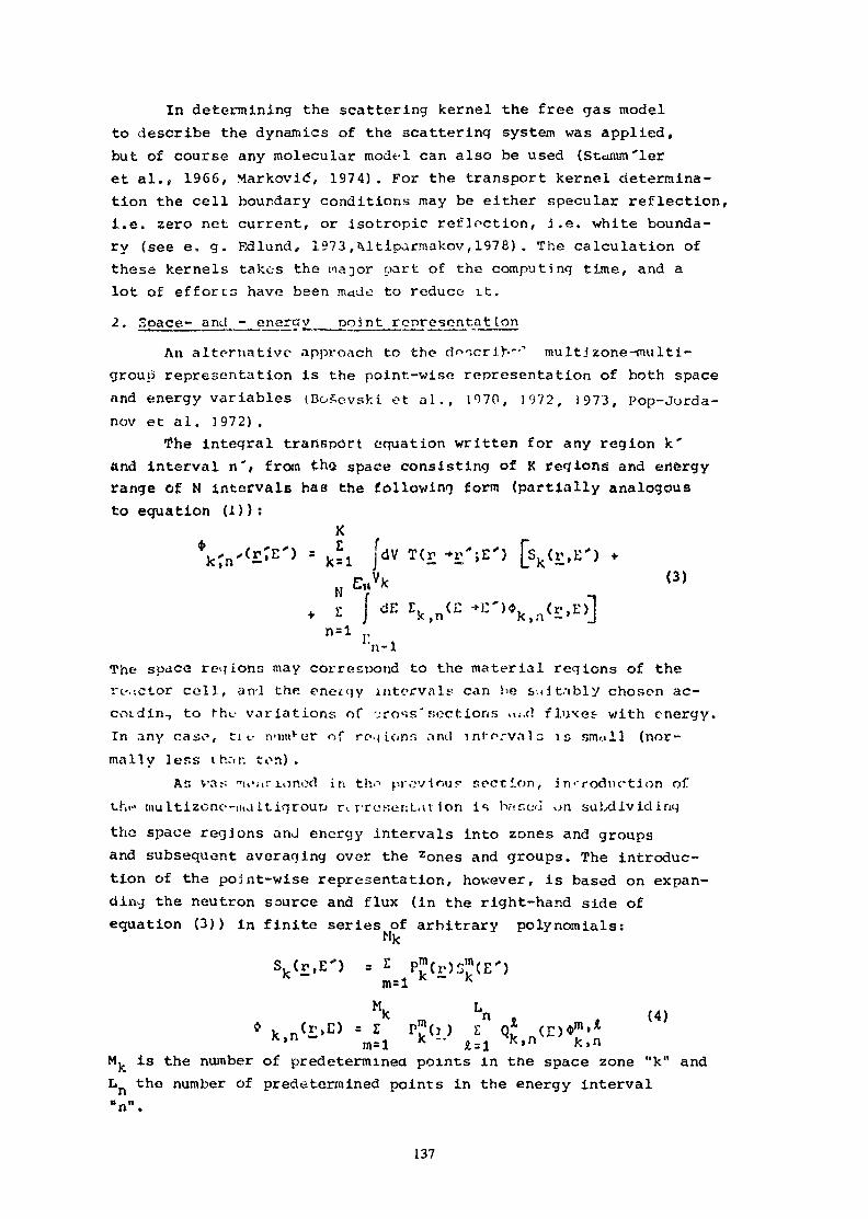
In determining the scattering kernel the free gas modelto describe the dynamics of the scattering system was applied,but of course any molecular modtjl can also be used (Stamm "1eret al., 1966, Markovic", 1974). For the transport kernel determina-tion the cell boundary conditions may be either specular reflection,1.e. zero net current, or isotropic reflection, i.e. white bounda-ry (see e. g. Edlund, 1973 »Mtiparmakov, 1978) . The calculation ofthese kernels takes the inaôr part of the computing time, and alot of efforts have been made to reduce it.2. Space- and_ - energy__POJ n t rpnrcsnntat Ion

An alternative approach to the d^criV-"* multj zone-multi-group representation is the point-wise representation of both spaceand energy variables (Boscvski et al., 1070, 1072, 1973, Pop-Jurda-nov et al. 1972) .

The integral transport equation written for any region k'and interval n', from the space consisting of K regions and energyrange of N intervals has the following form (partially analogousto equation (1)):

K* /„'r.*\ - =! JdV T(r

n=ln-1

The space regions may correspond to the material regions of therc-.ictor cell, an-1 the energy interval« can be su i tably chosen ac-cotdin-, to fhf variations oC -„TOSS" sections -«».d fluxet with energy.In any case, t i t - n>un v er of re.| lonn nncl int'e.-vnl a is small (nor-mally less ihnr. t on ) .

As vras "u'nr toned in tfv provinur section, in t roduct ion ofthe multizone-iiui Itiqroup r<. r - r o K u n L a t ion i<-> h<ir.uij ^n suSxJividinq

tho space regions and energy intervals into zones and groupsand subsequent averaging over the 2ones and groups. The introduc-tion of the pojnt-wise representation, however, is based on expan-ding the neutron source and flux (in the right-hand side ofequation ( 3 ) ) in finite series of arbitrary polynomials:

MkS. <r.,E-> = Ï Pm(r)5'n(E")

m=l k ~ k

* " M)M. is the number of prédéterminée points in tne space zone "k" andL the number of predetermined points in the energy interval

137

The distribution of energy and space points (within zonesand intervals) can be conveniently chosen with the aim of obtaining the most accurate integral reaction rate (Bosevski, 1970) .

Applying these expansions,, the integral transport equationis finally transformed into the following general linear algebraic form: K M,

[s-«-,

En(5)

E „n-1

• J dV T(r.r-»i:'>pm(r)t» K •—•Compared to the space-zone-energy group equations the same structur«is obtained avoiding the flat-flux and group-averaging approxima-tions.

Introducing in (5) successively all values of predeterminedspace and energy points, a system of £M. times EL linearalgebraic equatjons is obtained. The solution of this systemprovides discrete flux values at the chosen set of spacu andenergy points, i.e. expansion coefficients $ '

In this method (PEPT)several ontions arenintroduced:(a) For the spaco interpolation function there are?

- Option c.i.1: even degree in "r" :- Option a.2: Lagran<ja polynomial in even degree in "r":

Mk 2 2n (r '-rf)•î - -t 3- « «

(b) For the energy interpolation function there are:- Option b.l:. Lagrange polynomial form:

Ln

n- Option b.2: Laguerie polynomial treatment, as in ANTER

(Pop-Jordanov , 1963), resulting. in:

P s Qt (E) from b.lJV j îl

M (E) is Mexwellian.138

Table I demonstrates some results for heavy and light watercells. DISKRET is an approximate version of SEPT, correspondingto the mentioned option a.l« Disadvantage factors obtained bySEPT are compared with standard Collision Probability method (CP)and Carlvik'ä (1967) Discfete Integral Transport (DIT). As canbe seen, the convergence of SEPT is superior. In particular, evem9 points yield bettor results than 30 heavy water ci- 20 lightwatör zones of the standard CP method.

The results of the SEIT for the flux distribution in the Yu-goslav RA reactor cell (having nine material zones) have shown tobe in very good agreement with Monte-Carlo calculations (Koci<5,1974) .

Summarizing it can be said that SEPT method hns several fa-vourable characteristic}-,, resulting from the basic idea of seekingthe actual flux values ftt the corresponding space and energy pointsSomes of those advantages are related to physics, the other to nume-rica.

Concerning physics, the discretization principle eliminatesthe necessity of assuming mean flux values and constant nuclearproperties in space subzones, which is otherwise common to standardCP and orht'r multàône procedures. In addition, instead of group-averaged nuclear constants uned in multigroup procedures, the propoed approach requires only the basic energy-dependent data. Parti-cularly, an appropriate treatment of low-energy resonance is en-abled. All these characteristics contribute to an increase in theaccuracy of theoretical results and, in addition, enable directcomparison with experiments.

Concerning numerics, the number of space and energy pointsis less than a half of the number of subzones and groups, forthe same accuracy. Simultaneously, the energy transfer matrix doesnot depend on buznup, since no spectrum dependent group scatteringcross sections are involved.. As a result, the mathematical modelconverges very rapidly, which is particularly important for burn-up programmes, where lattice-spe.ctrum recalculation is necessa-ry (Pop-Jordanov, 1973) .

The collision probability applications described in this andthe previous section are based entirely on the integral tran-sport theory. However, it was shown to be very efficient to com-bine the collision probabilities (in the highly absorbing fuelregion) with other types of neutron balance equation (in the restof the cell). Two approaches of that kind, concerning thermalneutron range and suitable for inclusion in lattice cell burnupcodea/are» the numerical SPECTROX method (Leslie, 1963) and theanalytical ANTER method (Pop-Jordanov, 1965) . More details &ndsome extensions may be found in Stamm'1er ei al., (1966), while

139

the connections with coll burnup codes are quoted in Pop-Jordanov (1969).3 • Spaeu-poj.nt energy^group representation

An improved Space-Point Energy-Group Integral transporttheory method (SPEC) is developed and applied to the local andglobal calculations of the Yugoslav RA reactor. Compared to otherintegral transport theory methods, the SPEC distinguishes by":(1) the arbitrary order of tho polynomial, (2) the effective de-termination of integral parameters through point flux values,(3) the use of neutron balança condition as a posterior measure ofthe accuracy of the calculation and (4) the elimination of thesubdivisions into zones in realistic cases (Bosevski et al. , 1974, 1975« )

The study was performed on three test problems in plane andcylindrical geometry, as well as on the nine-region cell of theRA reactor (Table II). In particular, the limitations of the in-tegral transport theory including its non-applicability to optical-ly large material regions and to global reactor calculations wereexamined.

The transport coefficients T in the multiône-multi-Ki ,ggroup equation have non-zero values for all k and i (since in theintegral transport theory oach zone contributes to all other zones),

9so that the number of these coefficients is K*" for each energygrv/up g. In plane geometry the computing time will be proportionalto K , and in cylindrical geometry to K . Therefore, the multizoneiriEëgral transport theory is, in principle, unsuitable for thetreatment of optically large material regions, requiring a subdi-vision into a large number of zones. The problem is different inthe case of integro-differential methods, where only adjacent coeffi-cients are interconnected (Askew, 1972).

However, the introduction of the pointwise representationof the space variables with the polynomial interpolations providessome possibilities of accelerating the integral transport calcula-tions. Instead of subdividing the material regions iàto zones withspacially constant flux and source, in the pointwise collisionprobability representation (CPN) the neutron flux and source areapproximated by polynomials of N-th order, resulting in discreteflux valuos at the chosen set of space points. Consequently> CPUcorresponds to the standard (flat rlux) dollisioh probability ap-proach, the CPl to the "linc-ar" £lux approximation and the CP2to the three-point approximation.

The intc-.tral transport equation in the space-point energy-group (SPEGï représentation would be (Boëevski et al.,1974,

140

Pop-.Tordanov et al., 1975):R_ N^+l G

~~l p'-i I r 'P*'9 cT7=i r */ 9 '•*? r ' p ' f9 ' j f'p*-*rp,g(6)

r- l ,2, . . .R; p = 1 , 2 , . . . N +1-; y = 1 ,2 , . . .G

_ _ . , -

~

where R denotes the total number of material regions, and Nr theorder of the polynomial in the region r. This multipoint-roulti-Sroup equation is similar in structure to the multizone-tnultigroupequation, the flat flxix-and -source assumption being avoided.

Rearranging trie above equation (6) as to include into thesource term the scattering from other groups, small systems ofmultipoint algebraic equations for each energy group are obtained.The systems are suitable for solving by standard source iterationprocedure, Vvnich in our case has shown to be fast-convergent(2-3 iterations for cell criticality calculations).

Comparing the SPEC with other existing multigroup polynomialinterpolation methods (as the "linear" or parabolic flux interpola-tion) it should be mentioned that the difference between them is notonly in the polynomial order, but also in the procedure of determi-ning the integral parameters of the regions. Namely, in the SPECthe integral characteristics of the material regions are determinedby quadrature formulas of CJaussian type (thus minimising the neces-sary number of points). Therefore, the interpolation polynomialsof arbitrary order are used only to transform the integral equationinto a system of linear algebraic equations, and not for the inte-gral parameter's determination. These are determined by the nume-rical integration using the obtained flux values in the chosen set ofintegration points.

Another specific feature of the SPEC is that, contrary toOther methods, the neutron balance fcondition is not supposed tobe satisfied in advance. Consequently, the investigation of itsfulfilment serves as a posterior measure of the accuracy of cal-culation. In this way the necessary number of iterations in theburnup calculations of a given cell is reduced to one, while theother methods require at least three iterations.

Tables Itl and IV comprise the results of CPN and MonteCarlo calculations of the thermal neutron flux irt the RA reactoroeli. In the Monte Carlo eatintatiohfl of tha neufctfoh flux ifi «pacepoints, the point flux estimator teehnicjue had to be used, whllofor the mean flux values the standard weighted track length estima-tor was simply applied (Kocid, 1975).

The SPEC procedure was applied to the calculation of thespace and energy flux distributions of the same cell using 26

141

Bofsdarenko groups. The results 6or the resonance groups arc pre-sented in Fig. 1 The same procedure was used in calculatingtho infinite smltip] icatior) factor and the material bucklingfor different lattice pitches (Fi-f.2). The results for the materialbuckling are in good agreement with the expérimenta 1 values(Raiaic* et al, 1963) (except for very small lattice pitches, wherethe experimental values were disturbed due to tho small corein a large reflector).

The previous results, indicating the applicability of themultipoint integral transport theory to cells with optically largeregions, suggested the introduction of the SPEC method to theglobal reactor calculation. This step was additionally supportedby the satisfactory agreement (within 0.001 in keff)between the

CPN results for both the plane geometry and for the cylindricalgeometry (of large radius) simulating this plane geometry.

Fig. 3 shows some results obtained by SPEC for the two-group radial flux distribution of the RA reactor (lattice pitch13 cm). The influence of the central experimental channel is clear-ly pronounced.

It is commonly stated that the integral transport theory,contrary to the integro-differential one, is not suitable for theoptically large material regions and for the global reactor cal-culations. The multipoint approach seems to provide a good startingpoint to overcome these limitations of the integral transporttheory,

4. Some additional improvementsa) An effective method of solving integral transport equa-

tion with anisotropic scattering has been developed. Instead ofsolving the complete problem (as was done e.g. in the disserta-tion of Ligou, 1973 and Sanches, 1974), here only isotropic part ofthe flux was firstly determined, and then the equation correspond-ing to the correction has been solved. The idea is analogous tosolving the energy dependent problem in the ANTER method (Pop-Jor-danov, 1965) . In this way the system of linear equations has beendiminished, as well as the numbef of corresponding moments.

Applying thö Galerkin method, the moments for the anisotro-pic part of the flux have been represented in terms of isotropic oneexpressed through special functions. Thus, all moments can be cal-culated exactly and simply, avoiding numerical integration. Satis-factory results for escape probabilities were obtained (tiâdunovid,1977).

b) The error introduced by replacing the actual cell by aWigner-Seit2 cell with certain boundary conditions, especially

142

In case of closely packed reactor lattices, iß a subject of recur-ring interest and have been studied by many authors« An effectiveboundary condition based on the zero neutron current and fche zeroderivative of the scalar flux on the outer surface of the cylindri-cal cell was proposed (Altiparmakov, 1978). In this way the neutronflux distribution for an arbitrary boundary condition may be ob~tained by solving the integral transport equation for vacuum bounda-ry condition and «sing the neutron balance condition.

Disadvantage factor calculations of the Thie lattice cellsare carried out. Comparisons with the previous results obtainedby various boundary conditions and various methods for Wigner-Seitz cell as well as two-dimensional methods for actual cellare performed. The proposed boundary condition has shown to bemore effective and more accurate in respect to others, particular-ly in the case of small optical dimensions of the moderator.

In fast neutron transport calculations the effect ofboundary conditions becomes more prominent for the other typesof cells and the application of the proposed boundary conditionis particularly recommended.

c) In the frame of cooperation with Saclay, France, aprocedure for solving twodimensional integral transport equationusing Galerkin method has been developed. The procedure wasapplied to cells with plate fuel elements, in finite or infiniterepeating media, with or without internal symmetries, and assum-ing Isotropie sources and scattering (Stankoviski, 1977) .

Based on the developed procedure, programme TIVOLI has beenwritten, whose multigroup version is included in the well knownFrench code APOLLO.

The twodimensional integral transport equation was alsosolved using a double sampling Monte Carlo approach. A computerprogramme KASETA was developed and applied to light water assem-bly calculations {Kocid, 1979).

REFERENCES

Altiparmakov, D.V., On the boundary condition in cylindrical cellapproximation, IAEA TC Meeting on Homogenisation Methods in ReactorPhysics, Lugano, Switzerland, 13-15, Nov. 1978.Askew, J.R., In"Nuraerical Reactor Calculations", IAEA,Vienna (1972)>CBenzi, V., Cupini, E., De Matteis, A., Journal of Nuclear Energy,Parts A/B, 2£ 1(1966) 17«ßoäevski, T., Pop-Jordanov,J., IBK-598 (1967) .

143

Boäevski, T., An improved collision probability method forthermal-neutron flux calculation in a cylindrical reactorcell, Nucl. Sei. Eng. 42, 23 (1970).Bosevski, T., Dissertation, ETF Becgrad, Apri] 1972.Bosevski, T, Pop-Jordanov, 3., Solution of integral transportequation in space and energy points with polynomial interpola-tion, Numerical Reactor Calculations, IAEA, Vienna (1972), 329.Eosevski, T., Pop-Jorcanov, J., Fast convergent space-and-energy-points transport theory method, Trans, Am. Nucl. Soc.1_6, 133 (1973) .Bosevski, T., Altiparmakov, D., XVIII Jpgosl. konf. ETAN(1974) .Bosevski, T., Altiparmakov, D., XIX Jugosl. konf. ETAN (1975).

Carlvik, I., Calculations of neutron flux distributions by meansof integral transport methods, Rep. AE-279 (1967).

Edlund, M.C., in "Developments in the Physics of Nuclear PowerReactors", J.Pop-Jordanov, ed.,IAEA, 1973, p. 40.

Honeck, H.C., Nucl. Sei. Rny. «, 193 (1960).Kocid, A., uoc. CEC (74) 1, Ccntro di Calcolo, Roioqna (1974)Kocid, A., Annals of Nuclear Energy, 2_ (.1975) 555.Kocid, A., Trans. Ani. Nucl. Toe. ,31, 1^7^, p. 258.Leslie, D.C., J.Nucl. Fnocqy 11_, 293 (1063) .

Markov id ,M. I . Justification of Krieqor-Nelkin averaqin^j in aniso-tropic molecular vibration«, J .Phyn. R:Atom Moloc. Phys. Vol. 7,No. 9 (1974) , L305-1.309.

Matausek, M., ='oci(f, A. et al. NET-TDK Computer Proqrarm-e package,ÎBK-14G8 (1973 ) . Also IEK-1411.

Pop-Jordanov, J., Neutron Thorna i. Iznuion in Heterogeneous Reactor,

ITEF 133, MOSCOV/, Jan. I9i":3 (in ilussian) .

Pop-Jordanov, J., Proc. Intern.Conf. Peaceful Uses at. Energy,UN, New York, Vol. 2, 126 (1965).

Pop-Jordanov, J., Kernenergie £, 288 (1969).

Pop-Jordanov, J., ôSévski, T., Matauëek, M . V . , Stefanovid, D.,and Strugar, B., Theoretical methods for core parameters determina-tion in uranium-plutonium lattices, Peaceful Uses of AtomicEnergy, New York, UN Volume 9 (1972), 181.

144

Pop-Jordanov, J.in "Reactor Burnup Physics", IAEA, 1973, p. 72.

Pop-Jordanov , J., Lattice cell burnup calculation, A series oflectures to the IAEA Review Courr-e, Mol, Belgium, 7-l<J October1974. (Also: TehnJcka fiîk-;, Journal of Engineering Physics,XVII, 1977 , 3-34) .

Pop-Jordanov, J., PcSevski, T., Kode, A., Altiparmakov, D.,A study of collision probability and Monte Carlo approaches to in-tegral transport theory for heterogeneous media, IAEA SpecialistMeeting on Methods of Neutron Transport Theory in Reactor Cal-culations, Bologna, Italy, 3-5, Nov. 1975.

Radunovic", J.8. Integral neutron transport theory with anisotro-pic scattering, MSc Thesis, Faqulty of Electrical Engineering,University of Belgrade, 1977.

Raiaic", N., Takac, S., Markovié, H., BoSevski, T., Proc. IAEASymp. on Exponential and Critical Experiments, Amsterdam (1963)509.

Stamm 'Isjr, R., Takaî, S., Keiss, Z., Technical Reports SeriesNo. 68, IAEA, 1966.

Stankovski, 2., Two-dimensional treatment of nc-utron transportin heterogeneous modln hy Galorkin ' s me>thod, M:';c Thesis, Facultyof Electrical Cnqinecrinn , Univc-rsity of Felrjrado, 1977.

145

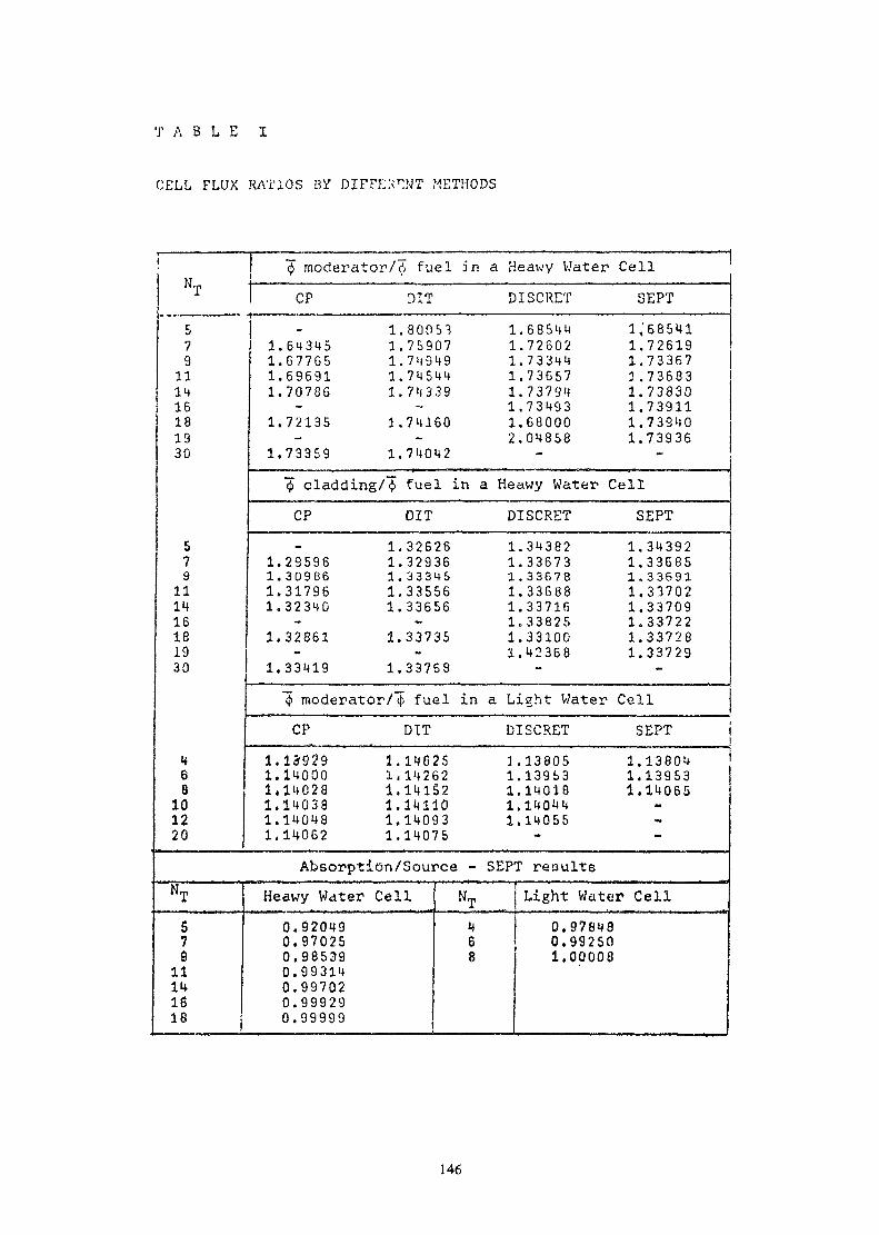
T A B L E I

CELL FLUX RATIOS BY DIFFEi^NT METHODS

moderator/Ä fuel in a Heawy Water CellNT579111416181330

579

111416181930

14e8

101220

* ~ '

CP DÎT1.80053

1.64345 1.759071.G77G5 1.749491.69691 1.745441.7078G 1.743391.72135 3.741601.73359 1.740421 cladding/"5 fuel inCP DIT

1.326261.29596 1.329361.30986 1.333451.31796 1.335561.32340 1.336561.32861 1.337351.33419 1.33768

"(f> moderator/1 fuel inCP DIT

1.13929 1.146251.14000 1,142621,14028 1.141521.14038 1.141101.14048 1.140931.14062 1.14075

Absorption/Source -NTS79

11141618

Heawy Water Cell NT0.92049 40.97025 60.98539 80.993140.997020.999290.99999

DISCRET1.685441.726021.733441.736571.737941.734931.680002.04858

SEPT1,'685411.726191.733671.736831.738301.739111.739401.73936

a Heawy Water CellDISCRET1.343821.336731.336781.336881.337161.338251.331001.42368

SEPT1.343921.336851.336911.337021.337091.337221.337281.33729

!a Light Water CellDISCRET1.138051.139S31.140181.140441.14055

SEPT resultsLight Water

0.978480.992501.00008

SEPT1.138041.139531.14065

M

Cell

146

TABLE ïiGEOMETRY AND COMPOSITION OF THE MATERIAL REGIONS OFRA REACTOR CELL

Region Material Outer Density Concentra-radius (cm) (p/cm ) i-0?, a(10 cm )

1 D20(0.25%H20) 1.05 1.105 D0H

2 Al 1.20 2.699 Al3 D20(0.25%H20) 1.45 1.105 D

0H

4 AI 1,55 2.699 Al5 U (2% U235) 1.75 18.700 U238

U235

6 Al 1.85 2.699 Al7 D20(0.25%H20) 2.05 1.105 D

0H

0 Al 2.15 2.699 Al9 D20(0.2S%H20) 7.3341l 1.105 D

0H

6.644893.330770.016656.029336.644893.330770.016656.029334.639140.095886.029336.644893.330770.016556.029336.644893.330770.01655

TABLE niTHERMAL NEUTRON FLUX IN SPACE POINTS OF RA REACTOR CELL

Radius (cm)0.00.8401.1251.2521.3971.5001.5641.6161.6841.736

H-C144.38142.08139.90138.21135.28132.67128.94127.72128.85133.57

CPN144.42142.31139.59138.68136.08132.29128.33127.21129.34

Radius (cm)1.8001.8922.0082.1002.2842.8323.7184.7895.860

134.11 6.748

M C-140.47144.59148.41150.29154.76163.55171.37177.50181.07181.59

CPN140.38144.23148.47150.58154.35163.18171.67177.57180.68181.65

147

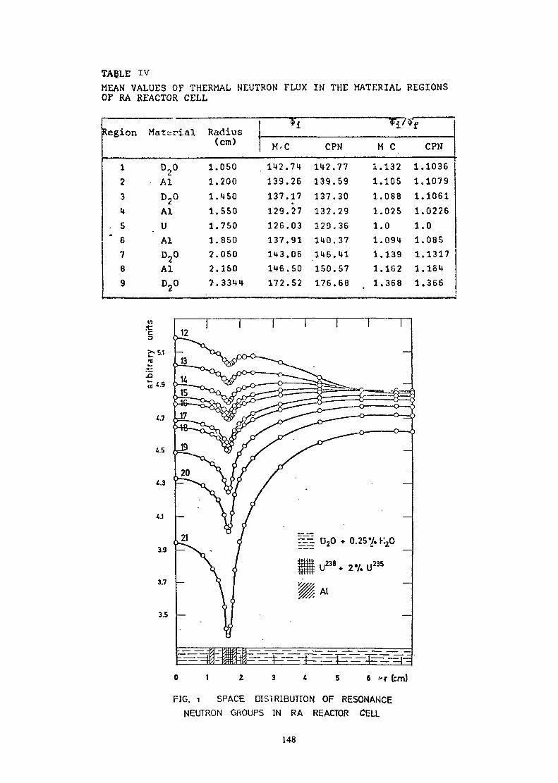
TAÇLE IVMEAN VALUES OF THERMAL NEUTRON FLUX IN THE MATERIAL REGIONSOf RA REACTOR CELL

Region

i234

. 567e9

Material Radius

D20• AlD20AlUAID20AID20

111111227

(cm)

.050

.200

.450

.550

.750

.850

.050

.150

.3344

*i *i/»f

M'. 142139137129126137143146172

C.74.26.17.27.03.91.06.50.52

CPN142139137132129140146150176

.77

.59

.30

.29

.36

.37

.41

.57

.68

M C111111111

.132

.105

.088

.025

.0

.094,139.162.368

111111111

CPN.1036,1079.1061.0226.0.085.1317.164.366

1 't (cm)

FIG. 1 SPACE DISTRIBUTION OF RESONANCENEUTRON GROUPS IN RA REACTOR CELL

148

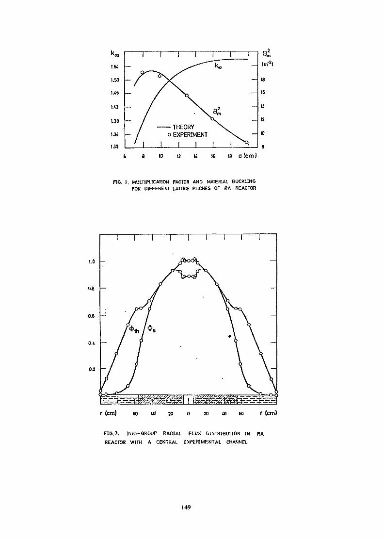
K»

1.54

1.50

1.46

1.42

1.38

1.34

UO

THEORYo EXPERIMENT

L I

Im"2)

ts16

U

12

10

6

io 12 u 16 is a (cm)

FIG. 2. MULTIPLICATION FACTOR AND MATERIAL BUCKLINGFOR DIFFERENT LATTICE PITCHES OF RA REACTOR

0.4 —

0.2 —

r (cm) 60 20 20 40 60 r (cm)

FIG.3. TWO-GROUP RADIAL FLUX DISTRIBUTION IN RA

REACTOR WITH A CENTRAL EXPERIMENTAL CHANNEL

149

INTEGRAL TRANSPORT METHODS

l . Integral transport theory and c o l l i s i o n p r o b a b i l i t i e s

The lattice cells of a power reactor are very complex,both In geometry and composition. Therefore It Is not possibleto obtain exact analytical solution of the Boltzmann equationfor this case. Accurate numerical transport theory approaches(as higher order S , P , C and also Monte Carlo) may becomeImpractical for repeated calculations In l a t t i c e cell burnupstudies, due to large computing time. On the other hand, thediffusion theory methods cannot be a p p l i e d , due to strong ab-sorbing properties and relatively small size (compared to themean free path) of the lattice cell components.

An effective approach to override these d i f f i c u l t i e s Inburnup calculations Is the use of c o l l i s i o n p r o b a b i l i t y methodsbased on Integral transport theory /I/.

The time Independent transport equation with Isotropiescattering may be written In the form:

00 Tr r r(r,E)= dVT(r-'r;E) S(r',E) + dE"£ (r' ;E'-*E— j — — L ~ i

VThe transport kernel T Is defined by:

which means the p r o b a b i l i t y (per unit surface) that a neutronof energy E o r i g i n a t i n g at r_" w i l l reach r_ without any col-lision. Consequently, the p r o b a b i l i t y for such a neutron tomake Its first collision In the volume dV about the point r_

w i l l be:

T(r"->r;E) « E(r,E)dV = P(r'+r;E) dV~ ~ ~ ~ ~ (3)

150

The optical path lengthT Is defined by:s"

T(r'+r;E) = f E(r-s"jB,E)ds" (i,)o

The above defined optical path length means sfmply the numberof collision mean free paths along the straight line between£ and r/; s'- /£-£*/ ;£ - - " -' .

IL - L"/The energy transfer kernel I(r_*J £•*• E) Is a macroscopic cross

section for collisions at r_* replacing a neutron of energy E*by the one having the energy E.

The Integral transport equation (1) Is often derived fromthe Integ rod I f f erent I a 1 transport equation, applying e.g. themethod of characteristics. Alternatively, It Is possible toobtain the Integral transport equation directly, using the de-finitions of kernels T and £, and considering the neutron con-servation. Namely, the second (Integral) term In the squarebrackets of equation (1) Is by d e f i n i t i o n the rate of collisionat r_* producing neutrons with energy E. Adding the source termand m u l t i p l y i n g by dV* yield the total rate at which neutronsemerge from dV* with energy E (from the source and from c o l l i -sions). M u l t i p l i c a t i o n by the transport kerrïel T (£'-»-r; E) andIntegration over V* give the total number of neutrons originatingelsewhere and arriving at r_ with energy E, wMch Is exactly

* (£,E).

(Analogously, the Integrod I f f erent la I transport equationmay be derived either from the LIouvMle equation, Introducingthe stoss Integral or directly, also considering the neutronconservation) .

The cell under Investigation may be derived Into K zones(each with spatially constant cross sections). The equation (1)then becomes:

««#.(r,E)a Z ! dV'T<r'-r;E> fs. (rsE) + T dE'Sv(E'*E)*v <r',E")11 ~ k=l Vv ~ " L * ~ J * * ~ J

151

where the Indices I and k denote Ind i v i d u a l zones related to r_and £_* respectively.

The average flux In I-th zone Is by definition:

vdv V£>E> (6)

If one assumes that the flux and the source within each ofthe zones are spatially constant, then *k(r.*. E") **ixÊ*) and

S. (r*,E) - T. (E). With this assumption the substitution of (5)K *— KInto (6) yields:

] IV

k=i IjkCE)+ 'V 'V dv« vi vk

The factor m u l t i p l y i n g the square brackets Is the transportcoefficient T.. . It can be expressed through the collision probabi 1 Ity Pk| , using (3) :

vkTki = ——— ~ ——— Pki 8Vi

where

Pki = —— dV dV'P(r'-r;E)

U s i n g (2) one may w r i t e :

Z.« (E) r t exp r-TCr^rjPki= — ——— dV dV" " ~i i . xV. i i i*ir|r'-

vk

(»0)

Consequently, the collision probability Pk, Is the pro-b a b i l i t y that a neutron originating with the energy E In the k-thzone w i l l make Its first collision In the I-th zone. Therefore,It Is called the first flight collision probability. It hasuniversal character and can be pre-calculated for a given geo-metry.

152

It should be reminded that the expression (10) Is v a l i dassuming Isotropie scattering In the laboratory system and spa-tial constancy of fluxes and sources within zones. In more generalcases the fluxes and sources dependent on r_*and Q_ appear.

Thus, by the c o l l i s i o n p r o b a b i l i t y method, In the flatflux approximation, the space~and-energy dependent Integraltransport equations (5) are reduced to merely energy dependentones (7). The obtained system of equations (7) can be and Iseffectively used for calculating the thermal, resonance andfast neutron flux and relevant parameters In lattice cells.

2. Spacezone-energyg roup representation

The energy dependence may be treated by standard mu 111 -group technique, which,In fact, Is an analogue In energy spaceto multlzone technique.

D i v i d i n g the whole energy range Into G energy groups onemay express the Integral over E* as the sum of Integrals overall the energy groups:

r G fdE' = I dE"J g'=i J£'

Substituting Into (7) the averaging over the g-th groupone obtains:

*'

where Indices g and g" denote the group averaged values.

The solution of this set of K x G algebraic equationsyields the mean flux values within the groups and zones, $ I .9(provided that the sources, scattering kernels and transportcoefficients are determined).

Of course, since the zone averaging and group-averagingtechniques are mutually Independent, the group averaging could

153

be applied to equation (1) before the zone averaging, or slmulta»neously wlth It.

The typical example of mu11lzone-mu11Igroup Integral tran-sport theory approach Is the THERMOS method /2/.A version ofTHERMOS has been used at the Boris Ktdrlc" Institute as well /3/.

In determining the scattering kernel the free gas modelto describe the dynamics of the scattering system was applied,but of course any molecular model can also be used M,5/. For thetransport kernel determination the cell boundary conditionsmay be either specular reflection, I.e. zero net current, orIsotropie reflection, I.e. white boundary (see e.g. /6,7/). Thecalculation of these kernels takes the major part of the com-puting time, and a lot of efforts have been made to reduce It.

3, Space-and-energy point representation

An alternative approach to the described mu111zone-mu111-group representation Is the point-wise representation of thespace and energy variables /8,9/.

The Integral transport equation (1) written for any re-gion k* and Interval n *, from the space consisting of K regionsand energy range of N Intervals has the following form (partial-ly analogous to equation (5)):

K* - '~'•*'^ - Z idv=i |

N+ In=l .,

n-1The space regions may correspond to the material regions of thereactor cel l , and the energy Intervals can be suitably chosenaccording to the variations of cross sections and fluxes withenergy. In any case, the number of regions and Intervals Issmall (normally less than ten).

154

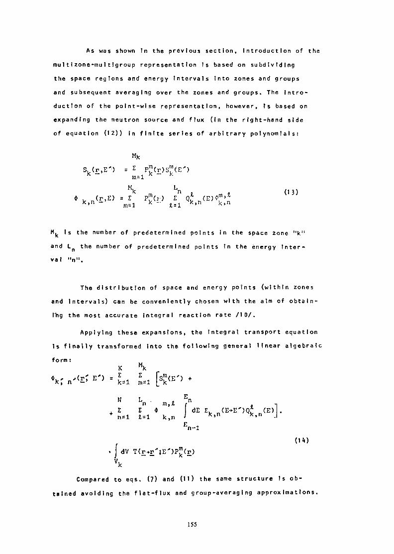
As was shown tn the previous section, Introduction of themu 1 t î zone-mu 1 1 ig roup representation Is based on subdividingthe space regions and energy Intervals Into zones and groupsand subsequent averaging over the zones and groups. The Intro-duction of the point-wise representation, however, Is based onexpanding the neutron source and flux (In the right-hand sideof equation (12)) In finite series of arbitrary polynomials:

S. Cr,E'> = £ pJ!<r>si"<E'>k ~ m=l * ~ kM T

(r, E) = l Pj(r) ^ Q* -(E)**»*' = * -• _ K, n k i n

M^ is the number of predetermined points In the space zone "k"and L the number of predetermined points tn the energy Inter-val "n".

The d i s t r i b u t i o n of space and energy points (within zonesand Intervals) can be conveniently chosen with the aim of obtaln-fng the most accurate Integral reaction rate /10/.

Applying these expansions, the Integral transport equationIs f i n a l l y transformed Into the following general linear algebraicform :

K Mkrx'x _ £ £n,=l

-n m,Ä t -,. I £ * dE 1. fl(E*E")Q* (E) .+ n=l £ = 1 k,n J k'n k'n -I

En-l(Hi)

. J dV T(r+r"}E")P r)Vk

Compared to eqs, (7) and (11) the same structure fs ob-tained avoiding the flat-flux and group-averaging approximations.

155

Introducing In (1 1») successively all values of predeterminedspace and energy points, a system of EM, times EL linear al-K ngebralc equations Is obtained. The solution of this system providesdiscrete flux values at the chosen set of space and energy points,I.e. expansion coefficients ft ' .*k,n

|n the SEPT-method several options are Introduced:(a) For the space Interpolation function there arc:

- Option a.1: even degrees In "r":

Pj<r> = A£ r2m"2

- Option a. 2: Lagrange polynomials In even degree In "r":MkH <r2-r?)

(b) For the energy Interpolation function there are:" Option b.l: Lagrange polynomial form:

L

- çn(Ej)J<

- Option b.2: Laguerre polynomial treatment (as In ANTER /11/,resu l 1 1 ng I n : -

^ n(E) =K,nn

P = Q (E) from b.l

M(E) Is Mexwel1 Jan.Table I demonstrates some results for heavy and l i g h t water

cells. DISKRET is an approximate version of SEPT, correspondingto the mentioned option a.1. Disadvantage factors obtained bySEPT are compared with standard C o l l i s i o n P r o b a b i l i t y method(CP) and Carlvlk's Discrete Integral Transport (DIT) /12/. Ascan be seen, the convergence of SEPT Is superior. In particular,even 9 points yield better results than 30 heavy water or 20l i g h t water zones of the standard CP method.

156

The results of SEPT for the flux d i s t r i b u t i o n fn the YugoslavRA reactor cell (having nine material zones) have shown to be?n very good agreement with Monte-Carlo calculations /13/.

Summarizing It can be said that SEPT method has several fa-vourable characteristics, resulting from the basic Idea of see-king the actual flux values at the corresponding space and ener-

gy points. Some of these advantages are related to physics, theother to numerics.

Concerning physics, the discretization p r i n c i p l e e l i m i n a t e sthe necessity of assuming mean flux values and constant nuclearproperties In space subzones, which Is otherwise common to stan-dard CP and other multizone procedures. In a d d i t i o n , Instead ofgroup-averaged nuclear constants used In m u l t l g r o u p procedures,the proposed approach requires only the basic energy-dependentdata. Particularly, an appropriate treatment of low-energy re-sonance Is enabled. All these characteristics contribute to anIncrease In the accuracy of theoretical results and. In a d d i t i o n ,enable direct comparison with experiments.

Concerning numerics, the number of space and energy pointsIs less than a half of the number of subzones and groups, forthe same accuracy. Simultaneously, the energy transfer matrixdoes not depend on burnup, since no spectrum dependent groupscattering cross sections are Involved. As a result, the mathe-matical model converges very rapidly, which Is particularlyImportant for burnup programs, where lattice-spectrum recalcula-tion Is necessary /1V.

The c o l l i s i o n p r o b a b i l i t y applications described In thelast two sections (*» and 5) are based entirely on the Integraltransport theory. However, It was shown to be very efficient tocombine the c o l l i s i o n p r o b a b i l i t i e s (In the h i g h l y absorbing fuelregion) with other types of neutron balance equation ( In therest of the cell). Two approaches of that kind, concerning ther-mal neutron range and suitable for Inclusion In lattice cell burnup

157

codes, are: the numerical SPECTROX method /15/, and the analyti-cal ANTER method /16/. More d e t a i l s and some extensions may be

found In Ref. /1?/ for SPECTROX and In Ref. /k/ for ANTER, w h i l etheir connections with cell burnup codes are quoted In /I 8/ and /19/,respect Ively.^• Space-point-energy group representation

An Improved Space-Point Energy-Group Integral transporttheory method (SPEC) is developed and a p p l i e d to the local andglobal calculations of the Yugoslav RA reactor. Compared to otherIntegral transport theory methods, the SPEG d i s t i n g u i s h e s by:(1) the arbitrary order of the polynomial, (2) the effective de-termination of Integral parameters through point flux values, (3)the use of neutron balance condition as a posterior measure of theaccuracy of the calculation and (*0 the e l i m i n a t i o n of the s u b d i v i -sions Into zones In realistic cases.

T.he study was performed on three test problems In plane andcylindrical geometry, as well as on the nine-region cell of theRA reactor (Table II). In particular, the l i m i t a t i o n s of the Integraltransport theory Including Its n o n - a p p l i c a b i l i t y to optically largematerial regions and to global reactor calculations were examined.

The transport coefficients T . In the mu111zone-mu11IgroupK l f yequation (11) have non-zero values for all k and I (since In theIntegral transport theory each zone contributes to all other zo-

2nes), so that the number of these coefficients Is K for eachenergy group g. In plane geometry the computing time w i l l be pro-

n 3portlonal to K , and In c y l i n d r i c a l geometry to K . Therefore,the multtzone Integral transport theory Is, In principle, unsulta,-ble for the treatment of optically large material regions, re-quiring a subdivision Into a large number of zones. The problemIs different In the case of l ntegro-dlfferentl a 1 methods, whereonly adjacent coefficients are Interconnected /20,2l/.

However, the Introduction of the potntwlse representationof the space variables with the polynomial Interpolations provides

158

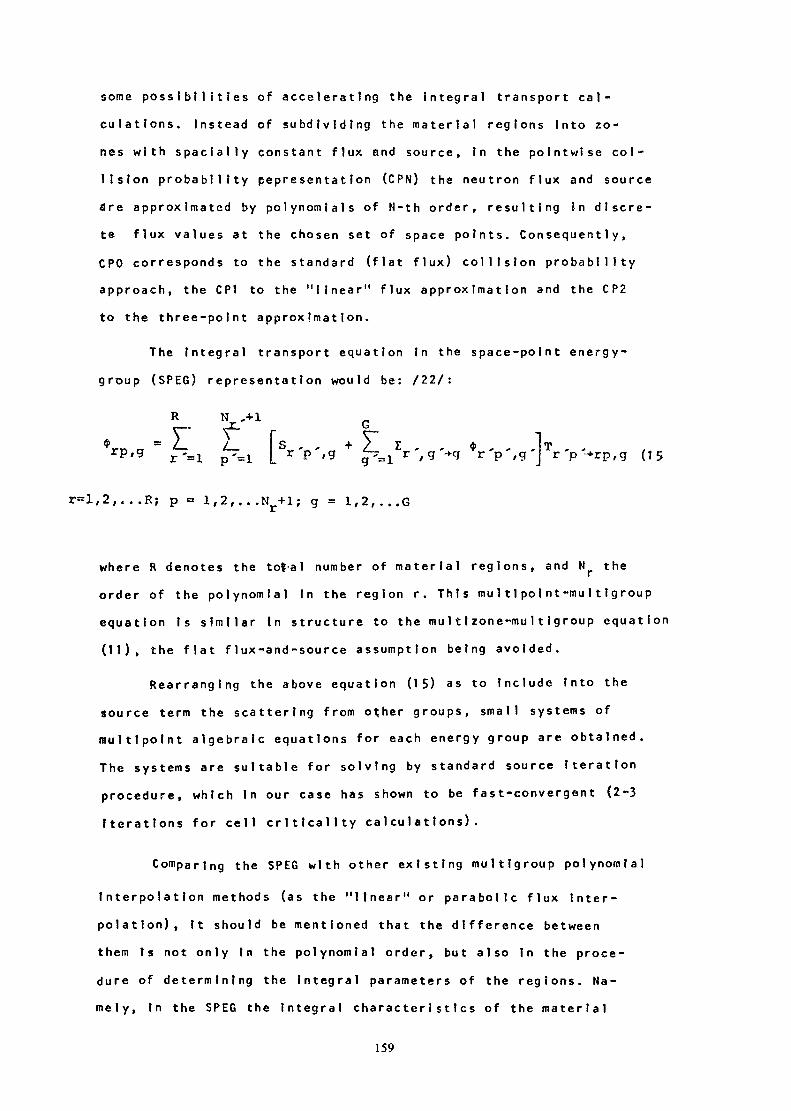
some p o s s i b i l i t i e s of accelerating the Integral transport cal-culations. Instead of s u b d i v i d i n g the material regions Into zo-nes with specially constant flux and source, In the polntwise col-li s i o n p r o b a b i l i t y pepresentat Ion (CRN) the neutron flux and sourceare approximated by polynomials of N-th order, resulting In discre-te flux values at the chosen set of space points. Consequently,CPO corresponds to the standard (flat flux) c o l l i s i o n p r o b a b i l i t yapproach, the CP1 to the "linear" flux approximation and the CP2to the three-point approximation.

The Integral transport equation In the space-point energy-group (SPEC) representation would be: /22/:

.*rp,9 = £T=I £r=1 [Sr 'p ',g + ^ r ', g '+g *r -p',g 'JTr 'p '-rp,g (1$

r«l,2,...R; p - l,2,...Nr+l; g = 1,2, ...G

where R denotes the tol'al number of material regions, and N theorder of the polynomial In the region r. This mu 1 1 1 pol nt-mu 1 1 Igroupequation Is s i m i l a r In structure to the mu 1 1 1 zone-mu 1 1 Igroup equation(11), the flat f lux-and-source assumption being avoided.

Rearranging the above equation (15) as to Include Into thesource term the scattering from other groups, small systems ofm u l t i p o i n t algebraic equations for each energy group are obtained.The systems are suitable for solving by standard source Iterationprocedure, which In our case has shown to be fast-convergent (2-3Iterations for cell c r l t l c a l l t y calculations).

Comparing the SPEC with other existing multlgroup polynomial

Interpolation methods (as the "linear" or parabolic flux Inter-polation), It should be mentioned that the difference betweenthem Is not only In the polynomial order, but also In the proce-dure of determining the Integral parameters of the regions. Na-mely, In the SPEC the integral characteristics of the m a t e r i a l

159

regions are determined by quadrature formulas of Gausslan type(thus m i n i m i s i n g the necessary number of points). Therefore, theInterpolation polynomials of arbitrary order are used only totransform the Integral equation into a system of linear a l g e b r a i cequations, and not for the Integral parameter's determination.These are determined by the numerical Integration using theobtained flux values In the chosen set of Integration points.

Another specific feature of the SPEC Is that, contraryto other methods, the neutron balance condition Is not supposed tobe satisfied In advance. Consequently, the Investigation of Itsf u l f i l m e n t serves as a posterior measure of the accuracy of cal-culation. In this way the necessary number of iterations In theburnup calculations of a given cell Is reduced to one, while theother methods require at least three Iterations.

The convergence of different c o l l i s i o n p r o b a b i l i t y approa-ches In calculating k ,, and the space flux distribution is shownIn Figs 1 and 2, respectively. The CPO, CP1 and CP2 approachesImply the s u b d i v i s i o n of material regions Into zones, whose totalnumber Is evident from the total number of points; In the CPNapproach no subdivision Into zones Is assumed. For a given totalnumber of points the subdivision Into zones results In the de-crease of accuracy.

The Monte Carlo calculations of k_*f are performed fol-lowing the procedure of réf. /23/, but instead of the weighted binomlal estimator, a flux estimator was used. This was done Inorder to make the definition of R ff consistent with that In thecollision p r o b a b i l i t y calculations.

The comparison of the results for the escape p r o b a b i l i t i e sobtained by CPN and by Monte Carlo are given In Table I I I . Theorder of the polynomials applied Is dependent on the opticalthickness of the medium, and Is verified by satisfying the neutronbalance condition. In the calculation of this benchmark, thesimple binomial Monte Carlo estimator Is found to be quite ef-ficient.

160

The results concerning mean flux values (benchmark No.3) arepresented In Table IV. Since E Is extremly large, the wholeabsorption occurs at the surface of the rod (In layers a fewmean free path thick). In this case It was necessary to subdividethe rod Into zones (two surface layers and the rest of the rod).In practice the strong absorbing rods are annular, and no sub-d i v i s i o n Into zones would be necessary.

The calculation of the mean flux values In the case of astrong absorber In large moderating media by the straightforwardMonte Carlo simulation would produce a large estimation variance.Since only a small percentage of the neutrons contributes to theestimator, a sophisticated Monte Carlo estimator Is needed. Theapplication of the weighted track length technique combined withthe unperturbed surface source resulted In a reduction of theestimation variance.

Tables V and VI comprise the results of CRN and Monte Caclocalculations of the thermal neutron flux In the RA reactor c e l l .In the Monte Carlo estimations of the neutron flux In space

points, the point flux estimator technique had to be used, w h i l efor the mean flux values the standard weighted track lengthestimator was simply applied.

The space and energy flux d i s t r i b u t i o n s of the same c e l lare presented In Figs 3-5. The SPEC procedure was a p p l i e d , using26 Bondarenko groups. The same procedure was used In c a l c u l a t i n gthe I n f i n i t e m u l t i p l i c a t i o n factor and the material buckling fordifferent lattice pitches (Fig. 6). The results for the mater i a lbuckling are In good agreement with the experimental values/2k/, (except for very small lattice pitches, where the expert-mental values were disturbed due to the small core In a largereflector) .

The previous results, Indicating the a p p l i c a b i l i t y of them u l t i p o i n t Integral transport theory to cells with o p t i c a l l ylarge regions, suggested the Introduction of the SPEC method

161

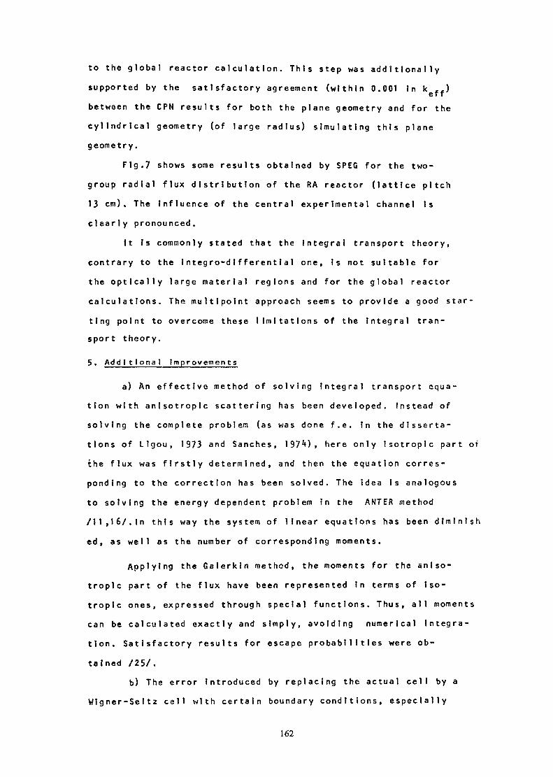
to the global reactor calculation. This step was a d d i t i o n a l l ysupported by the satisfactory agreement (within 0.001 In k ,,)between the CPN results for both the plane geometry and for thecylindrical geometry (of large radius) simulating this planegeometry.

Fig.7 shows some results obtained by SPEC for the two-group radial flux distribution of the RA reactor (lattice pitch13 cm). The Influence of the central experimental channel Isclearly pronounced.

It Is commonly stated that the integral transport theory,contrary to the Integro-d1fferent1 a! one, Is not suitable forthe optically large material regions and for the global reactorcalculations. The m u l t i p o i n t approach seems to provide a good star-ting point to overcome these l i m i t a t i o n s of the Integral tran-sport theory.

5. A d d i t i o n a l Improvements

a) An effective method of solving Integral transport equa-tion with anlsotroptc scattering has been developed. Instead ofsolving the complete problem (as was done f.e. In the disserta-tions of Llgou, 1973 and Sanches, IS?4»)» here only Isotropie part ofthe flux was firs t l y determined, and then the equation corres-ponding to the correction has been solved. The idea Is analogousto solving the energy dependent problem In the ANTER method/Il,l6/.ln this way the system of l i n e a r equations has been d i m i n i s hed, as well as the number of corresponding moments.

Applying the Galerkln method, the moments for the anlso-troplc part of the flux have been represented In terms of Iso-tropie ones, expressed through special functions. Thus, all momentscan be calculated exactly and simply, avoiding numerical Integra-tion. Satisfactory results for escape p r o b a b i l i t i e s were ob-tained /25/.

b) The error Introduced by replacing the actual cell by aWlgner-Seltz cell with certain boundary conditions, especially

162

In case of closely packed reactor lattices, is a subject of recur-ring Interest and have been studied by many authors. An effectiveboundary condition based on the zero neutron current and thezero derivative of the scalar flux on the outer surface of thecylindrical cell was proposed In /?/• In this way the neutronflux distribution for an arbitrary boundary condition may beobtained by solving the Integral transport equation for vacuumboundary condition and using the neutron balance condition.

Disadvantage factor calculations of the Thle lattice cellsare carried out. Comparisons with the previous results obtainedby various boundary conditions and various methods for Wigner-Seltzcell as well as two-dimensional methods for actual cell areperformed. The proposed boundary condition has shown to be moreeffective and more accurate In respect to others, p a r t i c u l a r l yIn the case of small optical dimensions of the moderator.

In fast neutron transport calculations the effect ofboundary conditions becomes more prominent for the other typesof cells and the application of the proposed boundary conditionIs particularly recommended.

c) In the frame of cooperation with Saclay, France, aprocedure for solving twodImenstonal Integral transport equationusing Galerkln method has been developed. The procedure wasapplied to cells with plate fuel elements, In finite or I n f i n i t erepeating media, with or without Internal symmetries, and assum-ing Isotropie sources and scattering /26/.

Based on the developed procedure, programme TIVOLI has beenwritten, whose multlgroup version Is Included In the well knownFrench code APOLLO.

REFERENCES1. J.Pop-Jordanov, Lattice cell burnup calculation, A series

of lectures to the IAEA Review Course,Mol, Belgium, 7-18October 197*». Also: Tehnlîka flzlka, Journal of EngineeringPhysics, XVI I (1977), 5-3^.

163

2. H.C. Honeck, Nucl. Set.Eng. 8, 193 (I960).3. M. MatauSek, A, Kocld, et al.. NET-IBK Computer Programme pack-

âge, IBK- 1468 (1978). Also IBK- 1411.

4. R. Stamm'ler, S. TakaC, Z. Weiss, Technical Reports SériesMo, 68, IAEA, 1966.

5. M.I. Markovld, Ju s t i f i c a t i o n of Kr Ieger-Nelkin averagingIn anlsotroplc molecular vibrations, J.Phys. B:Atom Molec.Phys. Vol. 7, No. 9 (197*0, L305-L309.

6. M.C. Ed1 und ,"Developments In the Physics of Nuclear PowerReactors"J. Pop-Jordanov,ed..lAEA,l 973 , p. 40.

7. D.V. A l 11parmakov, On the boundary condition In c y l i n d r i -cal cell approximation, IAEA TC Meeting on Homogen t sat ionMethods In Reactor Physics, Lugano, Switzerland, 13-15 Nov.1978.

8. J.Pop-Jordanov, T. Bolevskl , M.V. Matauïek, 0. Stefanovlc,and B. Strugar, Theoretical methods for core parameters de-termination In u r a n i u m - p l u t o n i u m lattices, Peaceful usesof Atomic Energy, New York, UN Volume 9 (1972), 181 .

9. T. BoSevskl, J.Pop-Jordanov, Trans. Am. Nucl. Soc. 16, 133(1973) .

10. T. BoSevskl, Nucl. Sei. Eng. 42, 23(1970).11. J. Pop-Jordanov, Neutron Therma1 IzatIon In Heterogeneous

Reactor, ITEF 133, Moscow, Jan. 1963 (In Russian).12. I. C a r l v l k , C a l c u l a t i o n s of neutron flux d i s t r i b u t i o n s by

means of Integral transport methods, Rep. AE-279 (1967).13.A.Kocld, Annals of Nuclear Energy, 2_ (1975) 555.14.J.Pop-Jordanov, "Reactor Burnup Physics", IAEA, 1973, p.72.15.Leslie, D.C., J .Nucl . Energy 1_7 , 293 (1963).16.J.Pop-Jordanov, Proc. Intern.Conf. Peaceful Uses at. Energy,

UN,New York, Vol.2, 126 (1965).17-.C.R. Mac Vean, A S i m p l i f i e d C e l l Theory Applied to the Cal-

culation of Thermal Neutron Spectra In Light Water Lattices,Rep. CURL-lo, Sept. 1964.

164

18.J.D. MacDougall, ARGOSY-'», A Programme for Lattice Calculations,Rep. AEEW-R kkS.

1 9« J . Pop-Jordanov , Kernenergie 9_, 288 (1969),20.G,t.Bell, S. Glasstone, Nuclear Reactor Theory, Van Nostrand

Relnhold Company,New York (1970) 366.2.1.J.R. Askew, In Numerical Reactor Calculations, IAEA, Vienna

(1972),p. 195.22.J, Pop-Jordanov, T. BoSevskt, A.Kode", D. Al tr I parmakov , A

study of c o l l i s i o n probability and Monte Carlo approaches toIntegral transport theory for heterogeneous media, IAEA Spe-c i a l i s t Meeting on Methods of Neutron Transport Theory InReactor Calculations, Bologna, Italy, 3-5, Nov. 1975.

23.V, Benzt, E. C u p i n i , A. De Mattels, Journal of Nuclear Energy,Parts A/B, 2J_ 1 (1966) 17.

2«».N, Rats'tc, S.TafcaS, H. Markovlc, T. BoSevskl, Proc. IAEA Symp.on. Exponential and C r i t i c a l Experiments, Amsterdam (1963) 509-

25.J.B.Radunovld, Integral neutron transport theory with anlso-troptc scattering, MSc Thesis, Faculty of Electrical Engineering,University of Belgrade, 1977.

26.2. Stankovskl, Two-dimensional treatment of neutron transportIn heterogeneous media by Galerkln's method, MSc Thesis,Faculty of Electrical Engineering, University of Belgrade, 1977.

165

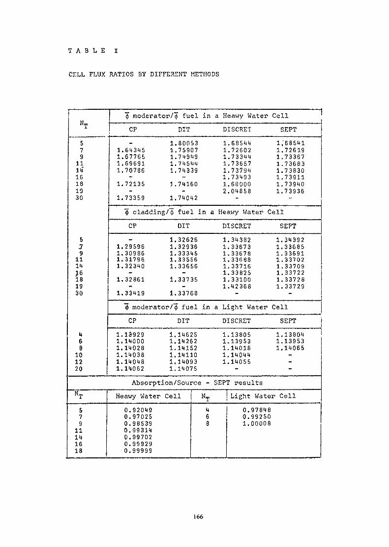
T A B L E I

CELL FLUX RATIOS BY DIFFERENT METHODS

1NT579

111416181330

5J911143-6181930

468

101220

(Ji moderator/ <J> fuel inCP DIT

\ ————————————————————1.80053

1.64345 1.759071.67765 1.749491.69691 1.745441.70786 1.743391.72135 3. 741601.73359 1.74042

~$ cladding/^ fuel in aCP DIT

1.326261.29596 1.329361.30986 1.333451.31796 1.335561.32340 1.336561.32861 1.337351.33419 1.33768

4> moderator/ <{> fuel inCP DIT

1.1S929 1.146251.14000 1.142621.14028 1.141521.14038 1.141101.14048 1.140931.14062 1.14075

Absorption/Source -NT57911141618

Heawy Water Cell NT0.92049 40.97025 60.98539 80.993140.997020.999290.99999

a Heawy Water CellDISCRET SEPT1.68544 1,'685411.72602 1.726191.73344 1.733671.73657 1.736831.73794 1.738301.73493 1.739111.68000 1.739402.04858 1.73936

Heawy Water CellDISCRET SEPT1.34382 1.343921.33673 1.336851.33678 1.336911.33688 1.337021.33716 1.337091.33825 1.337221.33100 1.337281.42368 1.33729

a Light Water CellDISCRET SEPT ;1.13805 1.138041.13953 1.139531.14018 1.140651.140441.14055

SEPT resultsj Light Water Cell

0.978480.992501.00008

166

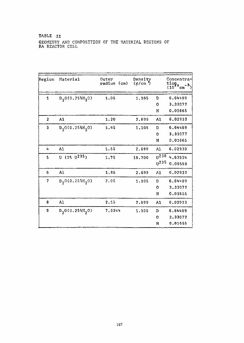
TABLE IIGEOMETRY AND COMPOSITION OF THE MATERIAL REGIONS OFRA REACTOR CELL

Region Material Outer Density Concentra-radius (cm) (p/cm 3) "tioc, *(10 cm )

1 D20(0.25%H20) 1.05 1.105 D0H

2 Al 1.20 2.699 Al3 D20(0.25%H20) 1.45 1.105 D

0H

4 AI 1.55 2.699 AI

5 U (2% U235) 1.75 18.700 U238U235

6 Al 1.85 2.699 Al7 D20(0.25%H20) 2,05 1.105 D

0H

8 Al 2.15 2.699 Al3 D20(0.25%H20) 7. 3341* 1.105 D

0H

6.644893.330770.016656.029336.644893.330770.016656.029334.639140.095886.029336.644893.330770.016556.029336.644893.330770.01655

167

TABLE IIIESCAPE PROBABILITIES FOR PLANE SLABS (BENCHMARK No.2)

N°sa N.

0.0001

0.005

1.

2.

3.

0.2

0.99900.99920.99920.99920.97670.97710.97690.97770.97770.1 R630.27550.18600.25640.27500.04810.15620.05140.11870.14720.01990.10050.01550.06530.0983

0.4

0.99930.99940.99940.99940.98240.982S0.98260.98310.98320.23420.33240.24260.31540.33280.07670.10380.07590.15220.18280.02710.1-2290.02510.07610.1228

0.6

0.99950.99960.99960.99960.98320.98850.98820.98860.98870.33390.42350.33680.40760.42400.12580.25250.12590.21200.24400.05010.16970.04800.12680.1650

0.8

0.99980.99980.99980.99980.99410.99420.99380.99420.99430.522]0.58670.51760.57820.59190.25990.38480.25870.34930.37950.12890.27110.12550.22270.2652

0.9

0.99990.999R0 .99990.99990.99700.99710.99680.99710.99710.6937

0.73770.68440.73100.73830.44050.54510.43610.51450.54040.26400.40700.26250.36310.4Q?1

Sources

P" d ,CP6PerPd,eP6T>' d,cD'S

Perd ,c

P6d ,cn" Sperpa,cp*Pd,cP6Perd ,c

P«Vd ,c

P6.Per' d ,c

Method

MC

CP1

MC

CP2

MC

CP4

MC

CP5

MC

CP5

168

TABLE ivMEAN FLUX VALUFS TM THE ABSORBING ROD AND THF MODFPvATOR(BENCHMARK 110.3)

NRod

1+5+51+6+61+7+7

Moderator

567

*rCPN

0.0349010.0351990.034914

MC

0.035006

EXACT

0.035

*m/*rCPH

5521•35585556

MC

5575

TABLE VTHERMAL NEUTRON FLUX IN SPACE POINTS OF RA REACTOR CELL

Radius (cm)0:00.8401.1251.2521.3971.5001.5641.6161.6841.736

M-C144.38142.08139.90138.21135.28132.67128.94127.72128.85133.57

CPN144.42142.31139.59138.68136.08132.29128.33127.21129.34134.11

Radius (cm)1.8001.8922.0082.1002.2842.8323.7184.7895.8606.748

M C140.47144.59148.41150.29154.76163.55171.37177.50181.07181.59

CPN i140.38144.23148.47150.58154.35163.18171.67177.57180.68181.65

TAÇLE VIMEAN VALUES OF THERMAL NEUTRON FLUX IN THE MATERIAL REGIONSOF RA REACTOR CELL

Region

123456789

Material Radius

D20AlD20AlUAID20AID20

111111227

(cm)

.050

.200

.450

.550

.750

.850

.050

.150

.3344

<J>i <*>i/$f

M-C142.139.137.129.126.137.143.146.172.

742617270391065052

CPN142139137132129140146150176

.77

.59

.30

.29

.36

.37

.41

.57

.68

M1.1.1.1.1.1.1.1.1.

C1321050880250094139162368

111111111

CPN.1036.1079.1061.0226.0.085.1317.164.366

169

keff

.15 —

1.10

1.05

1.00

0.9S

0 5 10 15 20 25TOTAL NUMBER OF POINTS

FIG.l. EFFECTIVE MULTIPLICATION FACTOR FOR A PLANE SYSTEM(BENCHMARK No. 1)

8 X (cm)

FIG ? SPACE FLUX DISTRIBUTION IN A PLANE SYSTEM (BENCHMARK No.1)

170

0 1 2 3 « 5 6 r (cm)

FIG. 3. SPACE DISTRIBUTION OF FAST NEUTRON GROUPS IN RA REACTOR CELL

0 1 2 3 4 s 6 r (cm)FIG. 4. SPACE DISTRIBUTION OF RESONANCE NEUTRON GROUPS IN RA REACTOR CFLL

171

4.3

4.1 —

3.9

1 r (cm)

FIG. 5. SPACE DISTRIBUTION OF EPITHERMAL ANDTHERMAL NEUTRON GROUPS IN RA REACTOR CELL

"00

1.54 —

1.50

1.46

142

1.38

1.34

1.30

- THEORYo EXPERIMENT

! l

R2Bm

Im'2)

18

16

14

12

10

10 12 14 16 18 Q (cm)

0.4 —

0.2 —

r (cm) 60 40 20 20 40 EO r (cm)

FIG. 6. MULTIPLICATION FACTOR AND MATERIAL BUCKLINGFOR DIFFERENT LATTICE PITCHES OF RA REACTOR

FIG.7. TWO-GROUP RADIAL FLUX DISTRIBUTION IN RAREACTOR WITH A CENTRAL EXPERIMENTAL CHANNEL

172

SOME FUNDAMENTAL RELATIONS BETWEEN CLASSICAL PROBLEMSOF TRANSPORT THEORV [1]

The simple use of the basic theorems of linear transport theory- complementarity and reciprocity theorems - allows to throw a bridge betweensome classical problems of one-speed transport theory, whatever the scatteringlaw is. Such very simple relations exist in the three one dimensional geome-tries : half-space, olack or grey slab, cylinder or sphere, surrounded by ahomogeneous and infinite scattering and absorbing medium.

Let us consider the three following problems :A. Current at infinityB. Constant production in the outer regionC. Entering current problem.A first series of relations connects the current J^(a) of particles

entering the black region at the boundary r = a (if the region is grey, J/\(a)is the global current of entering minus outgoing particles) , in problem A, tothe extrapolation distance of problem B, defined as

PB Ca]

where pg (a) is the asymptotic part of the global density in r = a, and p„ (a)its derivative.

In plane geometry the following relation was obtained1

J C a ) 2 Noo X V 'A 1 + n7

oowhere p.la) is the value at the abcissa x = a of the density at infinityf\

oo xp.(r) = exp (——)

where r)0 is the discrete eigenvalue of the transport operator in the outer (x>a)medium, and where N0 is the Case normalization coefficient

(3)

Eq. (2) holds whatever the medium x < a is, provided the same boundarycondition holds in both problems A and B. In particular, the medium x < a maybe heterogeneous. This allows to treat a slab C- -|, |-) for which the number

iIn the aase of the classical half-space Milne problem, this relation isequivalent to the one obtained, following another way,by Danison ([2],p. 79, Eq. 6.57) ; it is also easy to establish by the method of elemen-tary solutions, as shown by Siewert [3]. But, by these two methods, itseems difficult to generalize the relation to more cotnplicated problems,such as the slab problem, or cylindrical or spherical problems.

173

of secondaries per collision is Cj, placed between two scattering andabsorbing half-spaces. The problem A is defined as [4],[5]

oo ypfl(x) •* p.Cx) = exp (—) as x -»• <*>ft ft n0p.(x) ->• 0 as x •> °°A

In problem B, a constant source is placed in the two outer half-spaces [6],[7],[8]. If we consider the distortion factor

.6/2- rÜA J--» -6/2iJ -6/2

dxi -nA = — "^

PACx) dx

it is possible, using Eq, (2), to relate A to the extrapolation distance ofproblem B, defined by Eq. (1) at the boundary 6_

2

A =

Eq. (2) may be generalized to cylindrical ans spherical geometries.For a cylinder

JACa) 2 ir n„

where

and where I0, K0 and ^l are Bessel functions ; the factor N0 is still givenby Eq. (3).For a sphere

T , , 8 ir a2 NJACa)

withexp (-— )

npa(r] -

It was established as a corollary that, in any geometrythe extrapolation distance A« of problem A becomes equal to the

extrapolation distance Xß of problem B in the limit c •> 1, i.e. when thecapture of the outer medium tends to zero (a relation between X^Cc) and Ag[c)for any c was obtained in [8],[9], but only in the half-space problem).

174

A last group of equations relates problem B (or A) to problem C,where particles are introduced into the outer medium from the boundarysurface, according to an isotropia angular density. The asymptotic densitypas(r) .is, in this problem, proportional to

•yrexp (- ——) (plane)noK. (—) (cylinder)o riexp (- —3——————— (sphere)

cThe ratio ———— (where J (a3 is the entering current) determines the normaJâ)

lization of this asymptotic flux. This ratio is related to X_ byB

„as, ,P (a3c ^ (plane)Jc(a)

,+ , , iraJ (a)c

2 -\————————— (cylinder)

PcS(a) 1 1———*——————— (sphere)''l 4- LJ l~ f *î 4- -|__._-

References

[1] P. Benoist - Some Fundamental Relations between Classical Problemsof Transport Theory - Nucl. Sc. Eng., 68, 31 (19783.

[2] B. Davison - Neutron Transport Theory - Clarendon Press, Oxford (19573,[3] C.E. Siewert, Private Communication (1977).[4] M.M.R. Williams - Br. J. Appl. Phys., _1_6, 1841 (1965).[5] P. Benoist, V.C. Boffi, P. Grandjean.A. Kavenoky, V.G. flolinari,

C.E. Siewert and G. Spiga - Nucl. Sc. Eng., 66, 217 (1978).[6] C.E. Siewert, K. Neshat and J.S. Phelps III, Nucl. Sc. Eng., 64, 884

(19773.[7] M.M.R. Williams - Proc, Phys. Soc. London, 65, 413 (1965).[8] G.C. Pouraning - Nucl. Sc. Eng., _1j3, 239 (1963).[9] W.P. Patrick, C.R. McDaniel and A. Leonard - Nucl. Sc. Eng., 50, 388

(1973).

175

Chapter IV

INTEGRO-DIFFERENTIAL TRANSPORT APPROACHES

J. STEPANEK, J. ARKUSZEWSKI, V. BOFFI, M.V. MATAUSEK

4.1. INTRODUCTION

This chapter summarizes the work done in Italy, Poland, Switzerland andYugoslavia in the field of integro-differential neutron transport theory.It reflects different viewpoints in the handling of the subject.

Some of the methods are based only on the solution of the integro-differentialequation, others use only the integral form of the transport equation.

Use of the characteristic solution closely related to the integral equation(ARKUSZEWSKI et al.,(19T9)) seems to be a rather effective way to acceleratethe 2 dimensional discrete ordinates (Sn) transport methods and supress oneof the main disadvantages, the ray effect.

The advanced "Surface Currents" (MAEDER (1975)) and "Surface Flux" (STEPANEK(1979)) methods are based on the solution of both the integro-differentialand integral form of the transport equation. As long as the spatial fluxeswere considered to be flat in each region only the integral form of thetransport equation was considered. The solution seems to be the best methodof simple handling the higher order Legendre polynomials used toapproximate spatial and angular flux distribution.

The coupling of the B integral transport equations with the related Pequations retroves the greatest disadvantage of the P theory and closes thesystem of the Pn equations (LIGOU, STEPANEK (1971*)).

Therefore the method based only either on the integro-differential or onintegral equation will be rather rare in the near future.

4.2. ADVANCED SOLUTIONS OP THE 1 DIMENSIONAL INTEGRO-DIFFERENTIAL TRANSPORT EQUATION

In the frame of a physical scheme according to which scattering, fissionand external sources are all taken to have azimuthal symmetry, three linesof approach have been adopted with the following aims:

177

- A) Constructing - by standard perturbation technique - asymptotic solutionsto exactly critical problems of neutron transport theory, (in the stationa-ry monoenergetic case the analysis has been developed for both planeand spherical symmetry, and for both isotropic and anisotropic scatteringand fission. Both the polyenergetic and the time-dependent versions ofthe monodimensional plane case as well as the case of threedimensionalcritical systems have been considered. Numerical results have been ob-tained for various parameters of interest in reactor physics (BOFFI etal. (1977), BOFFI et al. (1977)).

- B) Handling anisotropy of scattering and fission for the case of generalboundary conditions and for different angular transfer functions ofscattering and fission, (in the stationary monoenergetic case the analysishas been developed for both plane and spherical symmetry, and for botha general and a "finite-order" anisotropy. Numerical results for variousquantities of interest in reactor physics have been obtained as functionsof a weighting parameter which accounts for the different anisotropicbehavior of scattering and fission (BOFFI et al. (1977)).

- C) Evaluating the flux depression factor due to a constant source, andthe flux distorsion factor relevant to a foil placed in an exponentiallyvarying flux. (The analysis and the corresponding numerical resultshave been processed for the stationary monoenergetic case with iso-tropic scattering and fission (BOFFI et al. (1978), BENOIST et al. (1978)).

The presentation of the above points will be restricted to the case of themonodimensional plane geometry (homogeneous slab of optical thickness 2aalong the z-axis). For further details the reader should refer to thebibliography.

A) Asymptotic solutions in neutron transport theory

When both scattering and fission are spherically symmetric in the laboratorysystem, the sourceless integrodifferential monoenergetic version of neutronBoltzmann equation reads as

" 3z X '"""" 2 X-1

(-Xa £ z £ Xa ; -1 £ y S l)

which is to be integrated using the symmetry

¥(z, y ) = ¥(-2,- y) (4.2.la)

178

and the boundary condition

f(Xa,u) =0 for p < 0 . (U.2.1b)

Introducing

«- s • •• ("-2-2)one gets

• ^ i f?>£L + f (x,p) - £c f(x,p')dp' (It.2.3)ep —* • • •*• i \.x,p;

-1

subject to the conditions

f(x,p) = f(-x,-p) ; f(|,p) =0 for p < 0. (U.2.3a)

As usual in perturbation theory, one seeks a solutionoo

f(x,p) = Z en f (x,p) . (It.2.It)n=0 j

For the total flux <j>(x) = 2ir f (x ,p)dp, we thus get

-1

OO

4 > ( x ) = Z en 4. (x) . (it.2.5)n=0

(For the coefficients f (x,p) and <f> (x) of the expansions in the r.h.s.of Eqs. (it.2.U)and (it.2.5), respectively, we observe that

fn(x,p) = fn(-x,-p) , <(>n(x) = <(>n(-x) (lt.2.5a)

as follows from the symmetry condition). Finally with00

c = z e cn (it.2.6)n=0

one deduces from Eq.. (it.2.3) the hierarchy of equations (n=0,l,2.... )

n+ fn(x,p) = Z c $ (x) (it.2.7)0 n-j

179

with f ,(x,vi) = 0. The general f (x,y), solution to Eq. (U.2.7), is

f(x,y)=j^ I (-1)* A .(x)u* , (U.2.8)

wheren-Si d <j) ._ .(x)

We need thus to determine the n+1 coefficients co, c , ..., c , and then+1 functions <ji (x), 4>n(x), ... $ (x). Multiplying Eq. (U.2.8) by 2iro -L nand integrating over ye (-1,1) we first verify that

c = 1 ; c = 0 , (U.2.10)o 1

whereas for n £ 2 we get for the general „(x) the second orderordinary differential equation

C2 <f>A(x) = G (x) , (z=o,i,....) (U.a.n)

dx

in which G (x) is a source term depending on c , c , . . .c andJO ^ J **

<j>0(x), (x), . . . ^ (x). The first few G 's are

GQ(X) = 0 G1(x) =

G2(x)(U.2.12)

In order to complete the structure of Eq. (U.2.11) the coefficients c , c ,..., cj.2 mus* e now determined. To do this, we impose on the general poly-nomial f (x,y), Eq. (U.2.8), instead of the rigorous boundary condition givenby the second of Eqs. (U.2.3a), the weaker condition

0

V = 0 , (U.2.13a)

-1

which expresses, as physically required, the vanishing of the net totalcurrent density entering the slab from the vacuum, and coincides with thefirst of the Marshak conditions so familiar in the theory of P- approxi-Jjmation. Using Eq. (U.2.8), Eq. (U.2.13a) becomes

n n-i rd <j> _._.(x) -t2 —— 2 c. ——n 3——d=o A+2 j=0 ° L dx -l l

.(x)(U.2.13D)

A+2 j=0

We thus infer that <j> (+ -)=0. Then Eq. (U.2.11) for A = 0 constitutes aneigenvalue problem. The eigenfunction corresponding to the lowest eigen-

180

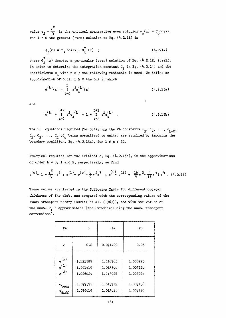
value e_ — is the critical nonnegative even solution $ (x) = C cosirx.For A > 0 the general (even) solution to Eq. (4.2.11) is

cosirx (x) ; (4.2.14)

where G (x) denotes a particular (even) solution of Eq. (4.2.12) itself.In order to determine the integration constant C in Eq. (4.2.14) and thecoefficients c with n % 3 the following rationale is used. We define asapproximation of order L fc 0 the one in which

L2A=0

(4.2.15a)

and

.(DLr (4.2.15b)

*=2

The 2L equations required for obtaining the 2L constants c , c, , . .., c ,Cn , C_, . .., C (C being normalized to unity) are supplied by imposing the-L c. Jj Oboundary condition, Eq. (4.2.13a), for l f n f 2L.

Numerical results: For the critical c, Eq. (U.2.15b), in the approximationsof order L = 0, 1 and 2, respectively, we find

(o) . ïï 2 (1) (o) 8 23 (2) (1)v '= 1 + — e ; c = c - — n e ; c = c ,16 2 It IK U ,, 0 .,.(— ir - — T ) e • (4.2.16)

These values are listed in the following Table for different opticalthickness of the slab, and compared with the corresponding values of theexact transport theory ( CUPINI et al . ( 1969 ) ) , and with the values ofthe usual P - approximation (the latter including the usual transportcorrections) .

2a

e

e<°>*™c<2>

beamCdiff

5

0.2

1.1315951.06lUl91.086029

1.0775751.079819

14

0 . 071429

1.0167851.0135881.013988

1.0137191.013835

20

0.05

1.0082251.0071281.007224

1.0071361.007170

181

B) Anisotropy of scattering and fission

The starting equation is

.. 3»(z.yi) _,_ _,,3z = S(z,y)

2ir

-1 0

, (U.2.17)

/ o owhere y = w' + /(1-y )(l-y' ) cos ($-$' ) is the scattering (or fission)oangle in the laboratory system, and n (y ) and II (y ) are the angular transferb O r Ofunctions for scattering and fission, respectively. Introducing the opticaldistance x = Iz, the mean number of secondary neutrons per collision

, and the function

n(y ,B) = BH (u ) + (l-g) n (y )O DU r O (U.2.l8a)

with

equation (k.2.17) becomes

3x f(x,y) = Q(x,y) + c (U.2.19)

-1 0

(-a $ x < : a ;

which will be integrated using the general boundary condition

f(Fa,vi) = h (y) for y < 0 . (i*.2.19a)

Actually H (y ) ^ IT (\i ). If, as usually done, one took II (y ) = II (y ),r O b O r o b o

then the dependence of Eq. (U.2.19) on 3 - which accounts for the different

anisotropic behaviour of scattering and fission - would disappear. In the

case of a finite-order anisotropy - which will be referred to - we have

Nn(y o ,ß) = l £S±i n n (ß )P n (y Q )

n=0(U. 2. 20)

with

nn(e)=3nSn+(i-3)nFn=2irn o (U.2.20a)

-I

P denoting the n-th Legendre polynomial.

182

In particular

n (e) = i n (u) = y(ß) =o JL (U.2.20b)

Once Eq. (U.2.20) is inserted in Eq. (U.2.19), the Green's function method allowsto put the problem, Eqs. (U.2.19) + (i*.2.19a), in the equivalent integral form

f+(x,y) = S+(x,y)P_(V)

n=0c y 4>n(y)dy , (i*.2.21)

Fa

where the subscripts + and - refer to the values for y > 0 and y < 0,respectively. In Eg., (if.2.21)

x±aS+(x,y) = e u h+(y) +-

_ .e y Q(y»y)dy (U.2.22a)

Fa

and

* (x) = 2ir P (y) f(x,y)dy . (U.2.22b)

-1Now, multiplying both sides of Eq. (U.2.21) ny 2ir P (y), integrating overye (-1, l) and summing up the resulting equations yields for the N-H un-knowns <j> (x) (m=0, 1, ..., N) the N+l linear integral equations

<(. (x) = S (x) + ± c E (2n+l)n (m m 2 nn=0*mn

-a

the known term S (x) of which is given by

Sm(x) - 2ir [ P(y) S_(x,y) dy -fm

-1

and the kernel by

dy

.2.23)

(U.2.2Ua)

im+n (x-y)y Pm(y) Pn(y)dy

The system of Eqs. (h.2.23) is now solved by integral transform method. Bytaking a Fourier exponential transform of both sides of Eq. (it.2.23) withrespect to x, we obtain

183

^ ^ N ^<f> U) = S (u) + c Z (2n+l)n (ß) k (u)m m 2 n mnn=0

sin[a(ijo-n)l <f>n(n) . (U.2.25)

Recalling now the Gegenbauer-Clebsch formula

,., , ,wo * * t-o

gai W' _ (k.8-aw

J (z) being the Bessel function of the first kind, and setting

m 4 (u) Z „(u) du ,m i (l».2.26b)

we infer that the general solution $ (u) to the system of Eq. (U.2.23) hasthe form

4) (w) = S (u) + c Z (2n+l) n (0) k (u) Z Ç Z. (u) ,m m 2 n mn n £ (U.2.27)

which is transformed back to yield for -a $ x. $ a.

N

n=0 i=0

.V2 k (x-y)P„(Z)dy. (l*.2.28)mn St a-a

This solution becomes explicit once the coefficients Ç , Eq. (U.2.26b ) ,areknown. For this purpose the solution for ij> (u), Eq. (it.2.20), is projected

m Ion the space spanned by the denumerable sequence {Z (oo)} and for the Ç , sthe following infinite system of linear algebraic equations is found

c t (2n+l) H (B) ZnC + B , (m, k = 0, l, ...) (U. 2. 29)n m

the matrix elements of which, A , are given bymn

(l|.2.3Qa)

and the known terms, B , bym

Bk =m S (u) Z, (u) dum k (U.2.30b)

respectively.184

Numerical results; Restricting our attention to the linearly anisotropiccritical case (N=l; h+(p) = h_(p) = Q(x,u) = 0; |p(ß ) | < —), the systemof Eqs. (4.2.23) reduces to

"X c, _ f<f>o(y) dy + | ey(ß) sgn(x-y) B2(|x-y|) 4'1

-a -a

» - c sgn(x-y) E([x-y[) 3 -

-a -a

whose approximate solutions of order N are

n=0and

2 2n+l

respectively. The coefficients Ç (n=0, l, ...2N +1) are in turn solutionsnto the system of 2N+2 linear algebraic equations

c«.. r x {<m mn nn=0

where X are appropriate matrix elements. Numerical values of the critical cmnare reported in the table below, for different values of a,vi , u , and (3 .b r

185

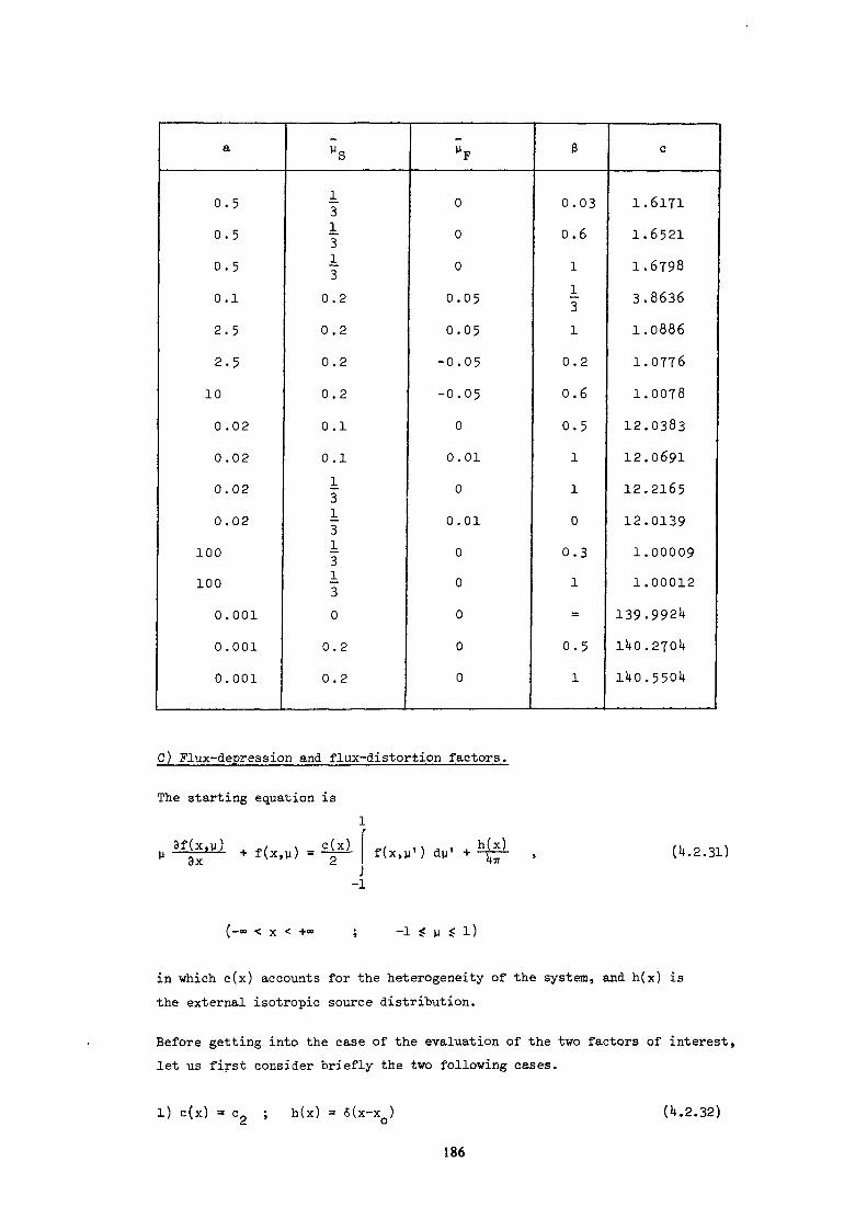
a

0.50.50.50.1

2.52.5

10

0.02

0.02

0.02

0.02

100

100

0.001

0.001

0.001

»S

1313130.2

0.2

0.2

0.2

0.1

0.113

I13Ï0

0.2

0.2

»F

0

0

0

0.050.05

-0.05-0.0500.01

0

0.01

0

0

0

0

0

ß

0.030.611310.2

0.60.511

0

0.31

=0.51

c

1.61711.65211.6798

3.86361.08861.07761.007812.038312.069112.216512.01391.000091.00012

139-992îko .270*11^0.5501*

C) Flux-depression and flux-distortion factors.

The starting equation is

-i(U.2.31)

(-00 < x < +°° ; -1 £ p £ l)

in which c(x) accounts for the heterogeneity of the system, and h(x) isthe external isotropic source distribution.

Before getting into the case of the evaluation of the two factors of interest,let us first consider briefly the two following cases.

c(x) ; h(x) = 6(x-xo) *.2.32)

186

This is the simple case in which the slab is homogeneous and of infinitethickness, and it will be taken as the unperturbed case of reference.For the total flux we have the well-known result

4>(x) s * (x) = g (x-x ) (U.2.33)xo 2 °With (U.2.33a)

. .t-, 2, | i f -a x-xa (1-a ) -a x-x , ' o1 ,/ } o o o1 o ' 1 I _____ e __________ . . . , da ,

«c2 x~V = r 2 ,. VI S 2 , C2 , vT1 2 A *£ «c2[ao -(l-c2)] j (1—— tanh -) + (- -f

tanh~1awhere a (|a |<l) is the real root of the transcendental equation l~c_ —————— = 0.It can be now noted that if for this unperturbed situation we want that thetotal flux ij>(x) E $ (x) for x -»• +°° assumes an exponential behaviour, that isxo °

then the source should be multiplied by a function of x , say Q(x ), equal to

c [c£-(l-c )] a0x0e , ( 2.35)

exponentially increasing with x .o

2) c(x) = Cgpa(x) (0<a<+«>) ; h(x) = 0 ( .2.36)

p (x) = U(x+a) - U(x-a) being the characteristic function of the finite&

interval (-a, a). In this case the slab is still homogeneous, but of finitethickness, and the external source is removed from the system. This is theclassical critical problem, involving the determination of the criticalvalues of c as functions of a, and of the corresponding eigenf unctionsfor both the total and the angular fluxes.

On the basis of these preliminaries we pass now to formulate the schemes forevaluating the flux-depression and the flux-distortion factors, respectively.

3) Flux-depression factor: let us set in Eq.. (U.2.31)

c(x) = c p (x) + c [1-p (x)l ; h(x) = 1 - p (x) . (It.2.37)J- Of £. I 9, I Si

187

With respect to the reference situation described by Eqs. (k.2.32), thiscase is perturbed by the presence of a foil placed between -a and +a (|x| < a,region 1, c < l), whereas a constant source acts on region 2 (|x| >a, c < l),which consists of the same material as in the reference situation. The objectiveis then to evaluate the flux-depression factor defined as

A = ——T^y < 1 (it.2.38)

for various combinations of c , c , a.

it) Flux-distortion factor: in this case in Eq.. (U.2.31) we take

c(x) = c p (x) + c [l-p (x)] ; h(x) = Q(x ) 6(x-x ) , (H.2.39)-L 8. ^ £L O O

where Q(x ) is given by Eq. (U.2.35)« With respect to the reference situationdescribed by Eqs. (k.2.32), this case is again perturbed by a foil of thickness2a placed across the plane x=0 (|x| < a, region 1, c < l), whereas a delta-like source is placed at x=x > a with an intensity exponentially increasingwith x and acts on the same material as considered in the reference situation.OAs x •»• -H» , the flux-distorsion factor is then defined aso

\=^TT ' (it.2.ito)

and will be evaluated for various combinations of c , cp, a.

The scheme for evaluating A and A, goes as follows. By Green's functionmethod we get for the total flux <j>(x) the linear integral equation

h(y)dy , (U.2.U1)c(y) E1(|x-y|) <j) (y)dy +

the Fourier transform of which is

(u>) = e(u,n dn+ £(<i)) , (It.2.1t2)

where for both cases 3 and h.

k(u,n) = (Vc2) gc (U) 3injftr)):1 ' (It.2.lt3a)

188

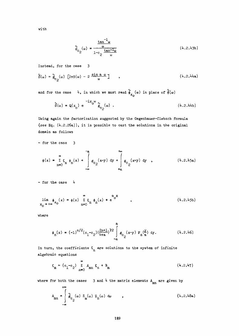
with

tan ta

Instead, for the case 3

&U) =S (««) [2irS(o,) -2

and for the case kt in which we must read $ (u) in place of 4(u)xo

S(<o) = Q(x ) eO (to) . (lf.2.UM>)

Using again the factorization suggested by the Gegeribauer-Clebsch formula(see Eq. (h.2.26&)), it is possible to cast the solutions in the originaldomain as follows

- for the case 3-a +00

= Z Ç 4 (x). n nn=0g„ (x-y) dy + (x-y) dy , (U.2.1»5a)

- for the case h

lim <j> (x) = 4(x) 1C 4 (x) + es ++00 xo n=0 n n

a xo (U.2.U5b)

wherear

4n(x) = (-l)-/2(el-c2)(|S±i)1/2 j gc (x-y) P J) dy. (U.2.U6)

In turn, the coefficients 5 are solutions to the system of infinitealgebraic equations

Ç = (c.-cj E A Ç + Bm 12 . mn n mn=0(U.2A7)

where for both the cases 3 and U the matrix elements A are given bymn ° J

Amn g (u) Z (u) Z (u) dw ,m n

189

whereas the known terms B are given bym

1-C2 mo

in the case 3, and by

anx _, /x\ ,e ° P (—) dxm a (U.2.U8c)-a

in the case U. Now we can verify that for both cases 3 and U

(U.2.U9)

so that the flux-depression factor A , Eq.. (U.2.38), is evaluated from

(U.2.50a)

whereas for the flux-distorsion factor Ai , Eq.. (4.2. 0), we have

-^ Jjo oir 2sinha ao

The problem is thus reduced to the evaluation of the coefficient Ç in thesuccessive approximations of order N, being n=N the finite term at whichthe infinite series in the r.h.s. of Eq.. (U.2.UJ) is truncated.

Numerical results: The values of A and A, for various combinations ofc , c and a are listed in the following table.

190

a

111110.0050.0050.0050.0050.050.10.250.5120.30.3

Cl

0.10.30.50.70.90.10.30.50.80.50.50.50.50.50.50.10.1

C2

0.80.80.80.80.80.950.950.950.950.950.950.950.950.950.950.950.975

A3

0.17130.20900.26880.37800.61*360.94630.95780.96950.98760.79230.66780.45950.30270.17710.09380.28420.2277

A4

0.35870.438l0.56380.79401.35390.94930.96080.97250.99070.81310.70100.51360.37260.26010.18820.32400.2492

4.3. DISCRETE ORDINATES INTEGRATED METHOD

4.3.1. Introduction

One of the main disadvantages of the discrete ordinates method in twodimensions is general discontinuity of the spatial derivatives to thesolutions on characteristics (ARKUSZEWSKI et al. (1972)):

The equation

in an rectangle M (Fig. 4.3.1) has a characteristic

(4.3.2)

determined by the origin. The solution to this equation on both sides of

191

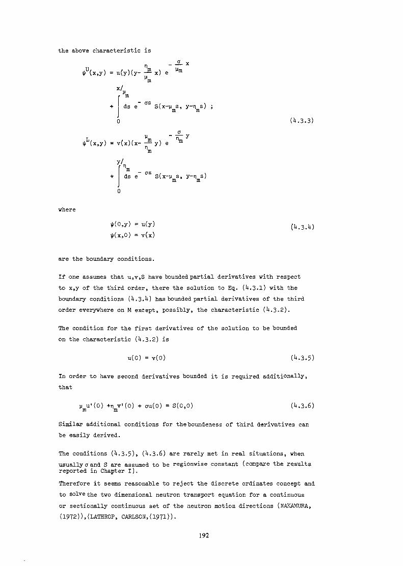
the above characteristic is_ _g_

* (x,y) = u(y)(y- — x) e m

\ds e S(x-y s, y-n s) ;m m

6 (U.3.3)g

*L(x,y) = v(x)(x-—y) e "»\

ds e S(x-y s, y-n s)m m

where

,y) = u(y) (U.3.U),0) = v(x)

are the boundary conditions.

If one assumes that u, v, S have bounded partial derivatives with respectto x,y of the third order, there the solution to Eq. (U.S.I) with theboundary conditions (U.S. M has bounded partial derivatives of the thirdorder everywhere on M except, possibly, the characteristic (U.S. 2).

The condition for the first derivatives of the solution to be boundedon the characteristic (U.S. 2) is

u(0) = v(0) (U.S. 5)

In order to have second derivatives bounded it is required additionally,that

U u'(0) +n v'(0) + au(0) = 8(0,0) (U.S. 6)m m

Similar additional conditions for theboundeness of third derivatives canbe easily derived.

The conditions (U.S. 5), (U.S. 6) are rarely met in real situations, whenusually a and S are assumed to be regionwise constant (compare the resultsreported in Chapter I).Therefore it seems reasonable to reject the discrete ordinates concept andto solve the two dimensional neutron transport equation for a continuousor sectionally continuous set of the neutron motion directions (NAKAMURA,(19T2)),(LATHROP, CARLSO»,(1971)).

192

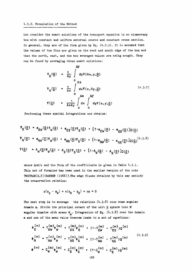
k.3.2. Formulation of the Method

Let consider the exact solutions of the transport equation in an elementarybox with constant and uniform external source and constant cross section.In general, they are of the form given by Eq. ( .3.3). It is assumed thatthe values of the flux are given on the west and south edge of the box andthat the north, east, and the box averaged values are being sought. Theycan be found by averaging those exact solutions:

Ay

° A x

Ax AjT

dxo o/o

Performing these spatial integrations one obtains:

*<£> - A w ( f l ) ¥ w ( Q ) * A8<fi)Vfi} * [,-yu, . A 8 ( 0 ) ] Q ( f l î

where Q=S/a and the form of the coefficients is given in Table 4.3.1.This set of formulae has been used in the earlier version of the codeTWOTRAN(X, Y ) (BARBER (1966)). The edge fluxes obtained by this way satisfythe conservation relation:

The next step is to average the relations (U.3.8) over some angulardomain m. Divide the principal octant of the unit JÎ sphere into Mangular domains with areas W . Integration of Eq.. (1+.3.8) over the domainmm and use of the mean value theorem leads to a set of equations:

* T(fn)*(m) * f1-T(m) -E EU W TES *S t1 TEW ESCm) m (m) (m) (m) (m) M.T(m) ,(m) (m)N 'NW *W TNS *S {1 TNW TNS )0

4 W193

where the transmission coefficients T and the penetration coefficientsC are defined as :x

T - ~ / d,ßa (fi)xy W J 2 xy —m(m).3.10)

The quantities $ m and Q m are the mean values of flux and source densityfor a domain m. According to the mean value theorem they are equal to theexact respective values taken at some point fi_ inside the domain.

Because of the quadratures over angles, that appear both in the definitionof the scalar flux and in source term, it is convenient to choose a singlerepresentative direction for each domain, constructing at the same time theset of domains in such a manner as to make the set of representative directionsidentical with the conventional discrete ordinates. This still leaves somearbitrariness in question how to divide the principal octant into domains.However, the symmetry properties of the (x,y) geometry allow to use themoment modified sets (BARBER (1966)), which have this additional advantageof constant domain areas.

The above approach is very similar to Nakamura's idea (1972) who proposedto span the solution on a finite set of sectionally defined "sphericalfunctions". The method presented in this paper uses in fact the sectionallynon-zero constants as Nakamura spherical functions. The problem of evaluatingtransmission and penetration coefficients is left open in his study.

A new CS technique developed by LATHROP and CARLSON (1971) is also similarto Nakamura's approach. They propose to use a modal expansion of the fluxin an entire octant and to evaluate the modal coefficients by moments method.A similar treatment is applied to the spatial dependence of the flux.

To evaluate the coefficients T , C the numerical integration has beenselected. In the case of the moment modified set all the domains, saveone, are rectangles in the variables

<(> = tan —Uand a direct quadrature formula can be used (KRYLOV et al. (1968)):

194

It has been found empirically that to obtain relative accuracy of the-Uorder 10 it is sufficient to use 1=9.

.S.3. A Numerical Example

As a numerical example a 19.05cmxl9.05cm supercell of the Shippingport PWRreactor (Fig. U.3.2) has been chosen. Since it was one of the first practicalproblems where the ray effects has been encountered, many studies devotedto it and now it can be considered as an unofficial "benchmark" problem(NATELSON (1971), LATHROP (1968), REED, LATHROP (1970)) for the two-dimensionaltransport calculations. Here 22x23 spatial intervals and S, approximationhas been used.

The ray oscillations are best seen on Fig. U.3.3, where DOT and DOIT fluxtraverses along the right edge and plotted. The traverse line is markedon Fig. U.3.2. A distinctive maximum can be seen in the DOT curve in thevicinity of y=10. Since it appears near the sourceless gap between blanketzones, this maximum can not be explained by any physical process. Especiallythe neutron streaming along the gap has to be excluded, since the crosssections in the gap and blanket zones are very close magnitudes. This isindeed a ray effect. Other irregularities in the flux behaviour can bealso attributed to rays propagation.

On the other hand, the DOIT results seem to be free of ray effects. Theonly questionable irregularity is a small minimum, which appears to theleft of material heterogeneity. The general lower values of the flux ascompared to the DOT calculated ones can be attributed to the DOT tendencyto overestimate the flux near the reflective boundary in a sourceless medium(compare Fig. U.S.2). The overall maximum value of the flux appear near thecenter of the seed zone and here the DOT value is 0.08786, the DOIT one0.0890U, while the "exact" calculation which is cited in Ref. (REED andLATHROP (1970)) (D-,/'» unknown number of spatial divisions: most probablyUUxU6)gives 0.08903. Here the DOIT accuracy is remarkable.

The total scattering rates for the whole supercell are in both calculationsvery close: 1.5913 (DOIT) and 1.5919 (DOT). This is an indication that thereaction rates are calculated correctly by both methods.Unfortunately the DOTprogram output options do not allow to print the reaction rates in variousmaterials. Even if the computer time for one point and one iteration isca. 2 times longer than for the DOT calculations, DOIT seems to requireless spatial intervals and less angular divisions as well as less iterationsto obtain the same accuracy. Then one can expect some actual computer timegains as compared to conventional discrete ordinate methods. This advantagehas been actually observed when running test problems. The main advantage,however, is the mitigation of the ray effects.

195

Since the longer computation times are caused by necessity to use discstorage device, it can be expected that implementing the DOIT code oncomputers with larger core memory will remove this deficiency.

1NW 5 " 5 (1

EW »,.-•

ES - .-«,

1 r » 1 r A ~ö, i[1- -M - e J] .Table U.3.1: Coefficients in Eq.. (U.3.8)

where a = aAx/yß = aAy/nP = a/ß

4.4. SURFACE CURRENT TRANSPORT THEORY IN X-Y GEOMETRY

A method for solving the neutron transport equation in x-ygeometry has been developed by MAEDER (1975)- In the interior and on theboundary of a mesh the flux depends linearly on the space variables. Theangular dependence is represented by a quadruple P.. expansion. The innerflux moments are determined from the basic form of the transport equation,while the mesh leakage is calculated by means of transmission and escapeprobabilities which are derived from the integral equation. Neighbouringmeshes are connected by requiring continuity of the angular current moments.Results calculated with the code QP 1, which is based on this theory, dependonly slightly on the chosen mesh division, and they are in good agreementwith more exact calculations.

196

U.U.I. Introduction

The EIR light water reactor fuel element program BOXER (MAEDER-PARATTE (1975))uses normally diffusion theory to determine the fine mesh flux distribution.To assess the accuracy of the diffusion approximation on selected configu-rations the transport program DOIT3 was built into BOXER. Because the DOITmethod (ARKUSZEWSKI (1973) and MAEDER (1973)) assumes a spatially constantsource within a mesh, its results turned out to depend too much on thechosen mesh grid. A new transport theory was therefore developed in whichthe neutron flux varies linearly in x and y in the interior and on theboundaries of a mesh. A quadruple P expansion is used in the four angularoctants formed "by the mesh boundaries.

The computer code QP 1, which is based on this theory, has been built intoBOXER where it replaces DOITS.

Section U.U.2- gives an overview of the QP 1 method, and QP 1 results arecompared with other calculations in section U.U.3.

U.U.2. Theory

The definitions of the quantities appearing in section U.U.2. can befound in the appendix and in the figures U.U.I.-U.

U.U.2.1 Flux moments

The system considered is divided into a number of homogeneous meshes asshown in Fig. U.U.I. First, the basic form of the transport equation

(H v-» + z) i|> (x,n) = s(x,n) (U.u.i)X

is multiplied by Y..(ß) P,(x) P (ï) and integrated over the neutron flightK.1L A p

directions (cf. Fig. U.U.2) and the mesh volume. Due to the mirror symmetrywith respect to the x-y plane one needs to consider only the upper half(0 >. 0) of the sphere formed by the neutron flight directions. In sectionU.U.2.2 the theory will be limited to a quadruple P expansion in the anglecoupled with a linear flux expansion in space. Therefore, the indices XukJlcan be restricted to the values 0000, 1000, 0100, 0001 and 0011.

After partial integration of the first term in Eq. (U.U.l) one obtains

,,/y _ {SAM _ TAu. , ._ . Ay (U.U.2)"

197

where

LAp -Lk£ "

and •"'

MXlJ - -Lk£ ZV

dA

2irdV

V

VY) ( U . U . 3 )

^ . U )

Here A is the mesh surface and fi the normal component of Q in the out-A

ward direction . In Eg.. (U.U.2) the following definitions of the flux andsource moments have been used:

;Xyk*2ir

f dV Px(X)Py(Y)

(U.U.5)

(U.U.6)

No approximation have been introduced in the derivation of Eq,. (U.U. 2) sothat it is an exact equation. The flux moments determined by means of Eq.(U.U. 2) will be used to calculate the source moments. Furthermore, the

, which are equal to the scalar fluxes in the meshes, form themoments ooidesired flux distribution.

The M-quantities needed in the theory may be derived from Eq. ( U . U . U ) :

„ooM, „ = 0

•£ • 2 C/ 'a (U.U.7)M.01•oo

To calculate the leakage term, Eq. (U.U.3), one divides the half sphereformed by the flight directions into the four octants of Fig. U.U.3 andcalculates the mesh leakage in each octant separately.

4 • Xy

wheref dfi Yk£(Ä) f PX(X) Py(Y)

(U.U.8)

(U.U. 9)

Let W, S, E and N be the mesh boundaries lying in the west, south, east

and north with respect to the flight direction. The leakage term may be

split into the contributions of the currents on the four boundaries.

198

-SX + <l)XwNX ~Wyq i.U.10)

where

C

(U.U.11)

(U.U.12)

qk*

w

(U.U.13)

(U.U.lU)

N EThe w - and w -coefficients may assume the values -1 or +1. Their definitionis given in the appendix.

U.U. 2. 2 Current moments

To calculate the neutron flux appearing in the definitions of the outwarddirected currents C and C , Eqs. C1*.1*.!!) and (U.U. 13), the integraltransport equation is used:

(5 ,2) e-Zso/C089.

The geometrical quantities appearing in this equation are defined in Fig.U.U.U.

The fluxes on the west and south boundaries through which the neutrons enterthe mesh are represented in the following form:

N Ä N-«,l l l

l=o k=o X=o

VV(U.U.16)

Note that the spherical harmonics are not orthogonal within an octant q. InEq. (U.U.16) the value of N may he 0 or 1. Eq. (U.U.16) is a quadruple Pexpansion of the incident boundary flux. The first angular moment (A=0) is

199

described more exactly in space than the higher moments. For the source anapproximation that is consistent with the definition of the source moments,Eq. (U.U.6), is used:

L £ N-£ N-£-X

i=o k=o X=o p=o• PX(X) P (Y) Yk£($)•

This equation defines *he spatial approximation of the source within the mesh.In the solid angle a P expansion (not a quadruple P expansion) is used,L Lwhere L is the maximum order of scattering anisotropy considered. Accordingto Eq. (U.U.17) N must be larger or equal to L. Thus the theory of this sectionallows linear anisotropy at most. If N is equal to 1, the source is a linearfunction of the space variables.

By applying the "pillbox" argument to the basic transport equation, Eq. (U.U.I),one may prove that the moments of the perpendicular currents are continuousat the mesh interfaces (MAEDER (1973)), pg. 17 and Chapter I of this monograph.

Therefore, it is advantageous to replace the inward directed angular fluxesappearing in the integral equation by the corresponding currents. If Eq.(U.U.16) is introduced into Eqs. (U.U.12) and (U.U.lU) and if the resultingexpressions are inverted, the following formular are obtained:

WX

SX

kX,N~vXv > k 'il1EX WX

Atr? !/• « P « U~V- I C I ' °

'i' Cqk'*(/aEX

(U.U.18)

The signs v are again defined in the appendix.

Finally the desired expressions for the outward directed currents may bederived by introducing Eqs. (U.U.15-U.U.18) into the definitions (U.U.11)and (U.U. 13). The result i-s

"qk£

NXw

EXw

r 01 N—!.' N— 5'— \ 'u n * w x, A k,£, ^NX, j,

r=o k'=o x'=o u'=o q q q

200

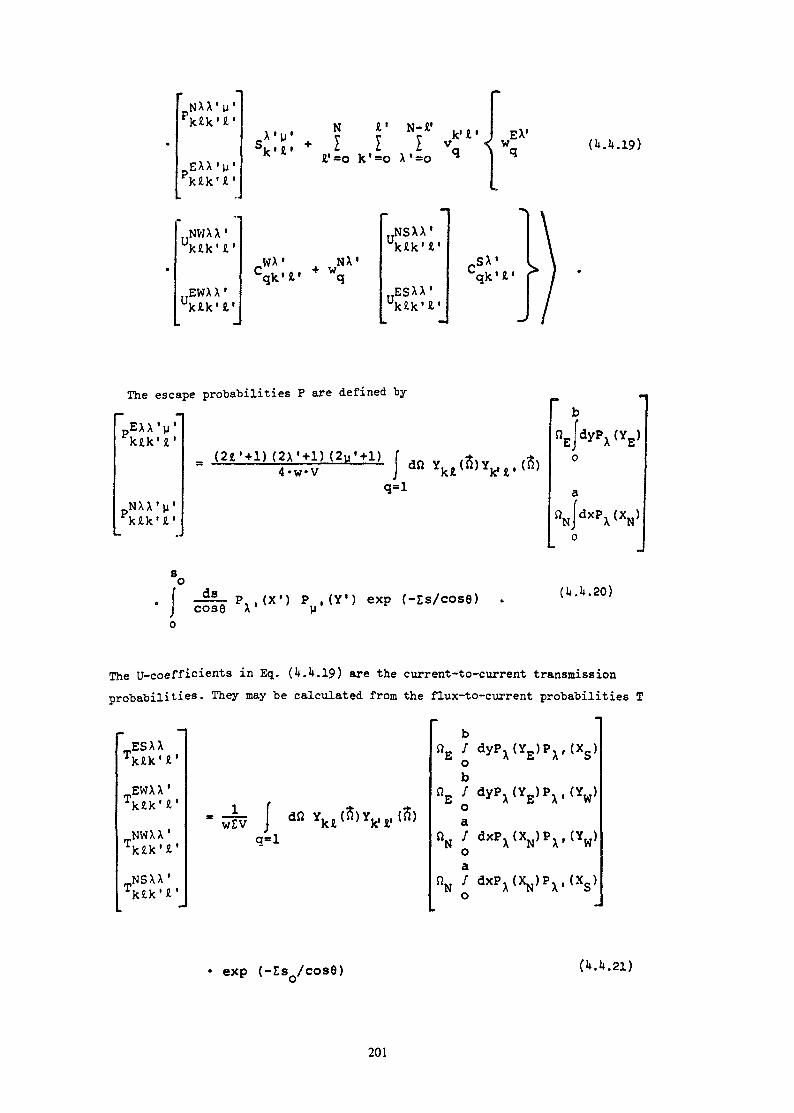
^J A A ^1pIf C. ' ß. '

p E A A ' u '

N W A A 1

Uklk'l'

E W A A 1U k £ k ' £ '

N O 1 M- {.« 1*• Si *• t i A t 1 M^À ' u ' r r r k1 i ' J E\s „ . + y > > v < wk ' A ' ' ' *• a »aK Ä'-o k'=o A ' = o H ] 4

WA1 + w NA'

..NSAA'kik'i'

E S A A 1

C SA-

(U.U.19Î

The escape probabilities P are defined by

p E A A VV 0 \r ' 0 I

..NAA'u1

(2£'+l)(2A'+D(2u'+l) fJq-i

,(X') P ,(Y') exp (-ZS/COS6) C*.«».20)

The U-coefficients in Eq. (1+.1».19) are the current-to-current transmissionprobabilities. They may be calculated from the flux-to-current probabilities T

.ES A A

E W A A 1

T. « 1.1 « i

_ N W A A '

N S A A '

a-1

Ob

oa

"N ; d x pA (V pA- (Vo

exp (-Zso/cos6)

201

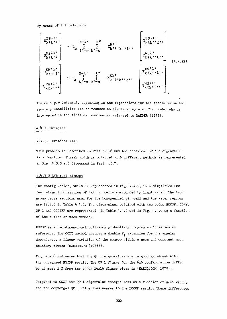
by means of the relations

ES**'

u:,NSAXT y y X N A >

b j r=ok»io x*'*'*"*"

E S X X -k J l k 1 ' l ' '

NSX(U.U.22)

UEWXX1

N W X X 'k £ k '

T f y X E X >a ^ ^ k ' i'le' ' f ' 'r'=0 k"=o K Ä

EWXX

NWXA»rk2k' '

Thf multipip integrals appearing in the expressions for the transmission andescape probabilities can be reduced to simple integrals. The reader who isinterest^ in the final expressions is referred to MAEDER (1975).

U.U.3. Examples

U.U.3.1 Critical slab

This problem is described in Part U.5.6 and the behaviour of the eigenvalueas a function of mesh width as obtained with different methods is representedin Fig. U.5.5 and discussed in Part U.5.7.

U.U.3.2 LWB fuel element

The configuration, which is represented in Fig. U.U.5, is a simplified LWRfuel element consisting of UxU pin cells surrounded by light water. The two-group cross sections used for the homogenized pin cell and the water regionsare listed in Table U.U.I. The eigenvalues obtained with the codes BOCOP, COXY,QP 1 and CODIFF are represented in Table U.U.2 and in Fig. U.U.6 as a functionof the number of used meshes.

BOCOP is a two-dimensional collision probability program which serves asreference. The COXY method assumes a double P expansion for the angulardependence, a linear variation of the source within a. mesh and constant meshboundary fluxes (HAEGGBLOM (1975)).

Fig. U.U.6 indicates that the QP 1 eigenvalues are in good agreement withthe converged BOCOP result. The QP 1 fluxes for the 6x6 configuration differby at most 1 % from the BOCOP l6xl6 fluxes given in (HAEGGBLOM (1975)).

Compared to COXY the QP 1 eigenvalue changes less as a function of mesh width,and the converged QP 1 value lies nearer to the BOCOP result. These differences

202

may be explained by the more exact basic assumptions used in QP 1. The angularflux is better represented by a quadruple than by a double P. expansion. Con-sider for instance the angular flux on a mesh boundary that lies perpendicularto a surface on which vacuum boundary conditions are imposed. There, the flux isstrongly peaked towards the outside of the system. It is not possible torepresent such a behaviour by a double P expansion. Furthermore, the COXYassumption of a constant mesh boundary flux is not consistent with thelinear dependence within the system.

Central processor computing times are listed in Table k.h.2. The BOCOP, COXYand QP 1 calculations were performed with diagonal symmetry, while no symmetryoption can be used in CODIFF at present. For the same mesh number CODIFF ismore than 10 times faster than QP 1. However, Fig. k.k.6 shows that CODIFF needsa greater mesh number to attain convergence.

The computing times of QP 1 and COXY given in Table k.k.2 are not directlycomparable because the calculations were performed on different computers.Assuming that the CDC 6600 computer is about twice as fast as the 6500 modelit appears that the COXY and QP 1 computing times are of equal magnitude.

.U.U. Conclusions

For the test problems described above the agreement in the eigenvalue and theneutron flux determined with exact calculations and with the QP 1 code is satis-factory. QP 1 shows a better agreement with the exact calculations and a smallerdependence on the chosen mesh size than diffusion theory or the new transportprogram COXY.

For the same mesh number the diffusion code CODIFF is an order of magnitudefaster than QP 1. Diffusion theory is therefore still needed to perform theroutine LWR fuel element calculations, while QP 1 can provide reliable checkresults within a reasonable computing time.

By introducing the general spherical harmonics Y (fi) defined in the appendixit would be possible to extend the theory of section U.U.2 to a quadruple P„Kapproximation with an arbitrary value of N. In such a theory the recursionrelations for the M-quantities(cf,Eq. h.h.2) and for the transmission andescape probabilities have a more complex structure. Such a theory has beendeveloped using orthogonal QPN Polynomials by STEPANEK (1979) and is describedon the example of the cylindrical geometry in section U.5

203

Appendix; Definition of Symbols

= cos9d9d<f> = Surface element of the unit sphere

Ki (x) = docos 6exp(-x/cos9) = Bickley function

P (x) = Legendre polynomial of order n

P£ (x) = Associated Legendre functionV = a-b = Mesh volumew = TT/2 = Surface of an octant

X = 2x/a-l = Dimensionless space coordiante in x-direction

Y = 2y/a-l = Dimensionless space coordinate in y-direction

' i j - 10

for i = ji * J

= Kronecker symbol

T = a£ = Optical mesh thickness in x-direction3

T, = b£ = Optical mesh thickness in y-direction

= P £ fv W = Spherical harmonics,

0 < k < 1, 0 < ?. £ N, 0 < m < £ , «,+m even,

im'

=cosm<}>

sinm*for

• m;2 d"'p— M —v ^ ——— -

k =0

1(x)

dx

Y, ç (tt) = Y, . f { n ) = Spherical harmonics used in QP 1,

0 < k < 1, 0 ^ 1,

Y = 1, Y = cos6 COS0, = cos6 siniji.

204

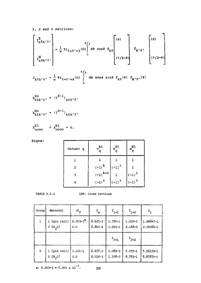
I, J and X matrices:

N

ÏÏ/2(*)

"/.a

EOk f c k ' A «

No = N-lk« .k '£ ' l ;

X E 1 * X N 1 =6oooo oooo

Signs:

Octant q

1

2

3

4

Vq

i(-i)k

(-Dk+i

(-D*

wqi

(-i)x

i(-Dx

NXwq

1

1

(-1)X

(-1)X

TABLE U . U . I LWR: Cross sections

Group

1

2

Material

1 (pin cell)2 (H20)

1 (pin cell)2 (HgO)

VZf

6.203-3a0.0

1.101-10.0

za8.627-36.8UO-U

6.957.28.016-3

j.1+1

1.780-11.995-1

W1.089-31.558-3

j.l-v2

1.002-22.188-2

«M

5.255-18.783-1

z*

1.966U7-12.2206U-1

5.96159-18.8787U-1

a: 6.203-3 = 6.203 x 10~3. 205

TABLE U.U.2 LWR problem: Eigenvalues and computing times

Program

COXY

BOCOP

QP 1

CODIFF

Mesh number

6x610x1016x166x6

10x1016x166x6

10x1016x166x6

10x1016x16

keff

1.21291 . 2lUO1.21U91.21751 . 2lU71.21381.21281.212lt1 . 212U1.21331.21821.2196

Computing time (s)total

6.919.26k.Q56.8

123-5292. h13. U32.583.90.81.76.0

probabilities

1.32.h5.6

Number ofinneriterations

323133

-U -3a: Convergence criteria for k = 10 and for the pointwise flux = 10QP 1 + CODIFF: CDC 6500 computer.COXY + BOCOP: CDC 6600 computer.

4.5- "SURFACE FLUX" TRANSPORT METHOD

U.5.1. Introduction

A new type of "surface currents" method to solve the one and two dimensionalneutron transport problems using Legendre polynomial approximation of the fluxin both angle and space, and the orthogonal Legendre polynomial or sphericalfunction approximation of the incoming and outgoing surface flux developed bySTEPAWEK (1979) is presented on an example for cylindrical geometry.

The X-Y geometry is currently developed by STEPANEK (1979). Originally, themain reason for developing the method for ID geometries was its very advanta-geous application for the computation of the neutron fluxes in the considerationof "pebble bed" structures of HTR fuel elements (STEPANEK(l978)). No lessimportant is also the efficiency of the method even for ID geometries, in com-parison to the other existing theories, and its consistent extension to 2Dgeometries, the use of orthogonal DPN Legendre polynomials to approximate theboundary angular fluxes, removes the inversion of the transport matrices andthe possibility of numerical errors (MAEDER (1975)) in cases of higherapproximation of the angular fluxes N.

206

Two codes based on this theory are developed. The first, SURCU, (STEPANEK(1979)), computes the neutron fluxes in homogeneous meshes for ID slab,spherical and cylindrical geometries and for 2D X-Y geometry. The second,SURCU-DH, (STEPANEK (1978)), computes the fluxes in ID slab, spherical andcylindrical geometries under the consideration of a "pebble bed" structureof the materials.

The ID space is divided into I space intervals (see Fig. U.5.1). Neutron sourcedensity approximations in angle and space using the Legendre polynomial ex-pansion are used in each interval. In contrast to the "mixed" method (LIGOUet al.(1972),(1973),(1973),(197*0, STEPANEK (1972),(1975)) and those of(TAKEDA (1973), PBEMUDA (1971),(1972), PREMUDA and TROMBETTI (1976)) nodirect transport connection between the intervals has been considered. Eachinterval is handled individually and connected to the neighbouring ones byincoming and outgoing surface flux. In contrast to Chapter k.k. (XY-geometry)these surface fluxes are approximated in angle using the orthogonal DPNLegendre polynomial expansions (YVON (1957), GREENSPAN et al.(1968)).

The general L, M and N orders of approximation for scattering anisotropy,neutron source space dependency and surface flux anisotropy are considered.The outgoing surface flux moments are computed for each interval from the volu-metric sources and from the incoming surface flux moments on the oppositeboundary of the interval, using the integral transport equation. Next usingthe integral and differential transport equation, expressions are derived for thevolumetric spatial Legendre polynomial flux moments in terms of the givenvolumetric sources and the incoming surface flux moments. Then the spaceLegendre polynomial flux moments are eliminated from equations for surfaceflux moments. This leads to a consistent system of equations for the incomingand outgoing surface flux moments for each space incoming and outgoing interval.The right hand side of the system depends only upon the given source moments.After solving this system, one eliminates the surface flux moments in expressionsfor volumetric spatial flux moments.

it.5.2. Theory (Cylindrical Geometry)

U.5.2.1 Integral Form of the Transport Equation

The integral form of the transport equation for the neutron flux *(r,fl} incylindrical geometry is (see Fig. U.5.1):

-*(r.5) - /ds q(r'.fl) l + » ( . f l ) e"cos6

207

where $(r,n) is the neutron angular flux, q(r,n) is the volume angular source,$(r ,n) is the neutron angular boundary flux and £ is the total macroscopic

ocross section and is considered to be constant inside of the space interval.

The q.,$ and the given angular volumetric source Q are expanded into the seriesof spherical functions:

(2n + 1 )-4Ü-

n = o n'=0,1£nn'

where

. 2 (n -n 1 ) ;nn> <1 + 6„iJ (n + n 1 ) :e

• n n , v » J L.USM ? rn is inoj , (U.5.U)

and

o ^7 j n r , .P (z)

dz"

The angular moments q. , , $ ,and Q , are defined by

fr,«).

where dû = cosQ d0 d^.

The total volumetric angular moments are given by

The boundary angular fluxes are expanded in the angular half spaces 1 and 2(see Fig. U.5.2) into the series:

n-o n'»o208

for - J « * < f. - ; s e < J .

and

n«o n'»o

for f S * s f ir. - | < 9

The polynomials Y are orthogonal in half spaces (-"£<$ < ~Z » ~^1® < 7Jand (TJ < <t> < ~Z v, - — < QfT;). The desired orthogonality property is

ir/2 ir/2f fd(ji -1 I0 0

„

The polynomials are calciilated using the power series

n Min(m,n+n'-m)r-v ^,(9,<(i) - ) /11 L^ L^YC .nn' j_ _ t L __ f nn

m=0 m'=0,l

the coefficients C are computed using the Gramm-Schmidt ' s procedure (MAEDERand STEPANEK (1978),STEPANEK (1979))-

1 2The surface flux moments ij> and <j> are defined by

ir/2 ir/2

< P ' ( r ) = 4 d* de cosen n ' Bo o

ir/2d* /

7F/2 O

irCpnn ( ( rB ) " 4 / d* / d9 cose Y^, (0 . * -$ ) »(r nî

The space is devided now into I space intervals (see Fig. U.5.1) and the crosssections are considered to be constant in each of them. The spatial distribu-tions of a ,(r), 9 ,(r) and Q ,(r) is approximated by Legendre polynomialsources in each interval:

' r

1-(n+n f)/2

. . (fc.5.10)V"O

209

where

y - (2 (—)ro

r.

<-) -B. (H.5.11)

A -A - ———

1+Ct

1-a2 '

(U.5.12)

q nn 'v "

nn ' v

0k. n n ' v _

1 T r n>r = v J dv (— ] p v ( y } 'V °

f 1nn'

$ , (r)nn

^nn' ^

(U.5.13)

where dV = 2rr r dr.

The spatial moments (q_ , ,« , and Q , ) and (a . ,* . and Q , )f Tin'v nn 'v nn'v Tin1v nn'v nn'vare connected by

nn ' v

.°nn'v,Z en'

Yvv'v = o

$nn 'v 'n

v. w nn 'v ' J

(U.5 .1U)

where y matrix is defined by

Y ° m = i dv (ï- )2mP (Y) P ( Y ) .jjv v r y vo

The computational method is pointed out by LIGOU et al. (1972),(1973),STEPANEK (1975),(1979).

Using Eg. (U.5.7) and (U.5.13) one gets the expression

qnn'v nn'v * Zsn *nn-v • (U.5.15)

where Z is considered to be constant inside the interval i.sni2 ft!Using £4. (U.5.1) the boundary moments $ , and $ , on the inner and outernpn SUM

boundary of the space interval are computed for 0 < m < N, O < m1 < m.

210

Setting Eq. ( .5.2), (1*.5.8) and (1*.5.10) into Eq. (U.5.1) multiplying itfey Y° , (6t4>-) or by Y° .(®»* ) and integrating of over 0 < <fr < -5-, or^-<*Bffli ^ nun o ™ — £ cand over 0 < 0 < — , one gets after rearranging (see Fig. U.5 .U) :

12 1 A n- «.„„.,.„

de m i nn Cos90 si o

2^ Z Z C 2 n + 1 ) Wn-n-V'n-n-n-

n ' « o

de cose Y m m , ( 6 ,$ . ) Y + , , ce .$ ) e ~ ~ ~ c o 7 ë , (U.5.i6)o

and*- s > l l ^ n ^

e - i Z < ^ ' X E n - ï

n M - ( n + n ' ) / 2q ,^nn'\>

n*o n ' =0,1

S° n' n's (— fo

SSo ' n' ïï/2

/°ds- (f )° P v t y j / de Y = m , ( e ^ o ) Y n n , ( 6 . < i > ) e - E ( s a - s > ] )s.

*ÎI Zn»o n'»o

TT/2 ff/2 ^0

*Q I dePo

N n\ \ ro-. j . ' *^ »^

Z Zn»o n'»o

* n * n ' n - n ' n ' n - n '

Cos6/ d6 0088 Y^.O.^J Y^^^.O.^) 8 COSO . (U.5.17)

0211

where s' = r'cos<f>', si = r^cosfjK, so = rocos<j»o.$8 » arcsina.

U.5.2.2 Differential Form of the Transport Equation

The differential form of the transport equation for the neutron flux*(r,^)inside of one space interval in cylindrical geometry has form (see Fig. U.5.1):

cose COS(>

vhere q and £ are total volumetric: source and total macroscopic cross section,respectively.

Multiplying this equation with Y ,, integrating it over ß and using Eqs.(U.5.6), (U.5.33), (U.5.3U), (U.5.35) one gets

, ( D -rn ' +1q , C r) .

(U. 5. 19)1 2where J and J , are the current moments in halfspaces 1 and 2, rtjsp.

(see Fig. U.5.2).

They are defined byir/2 ir/2

3'{r) = 4 d* cos* d9f d* cos* fo o

( U . 5 . 2 0 )n, IT TT/2

(-D 4 J d<{. cos* /" de cos2e Y n n , cn ) »tr.nj .TT/2 O

Multiplying Eq. (1+.5.19) by 2ir P (y)/r and integrating it over r by partsone finds after use of Eq. (U.5.20), (U.5.33), (U.5.31), (^.5-32), (U.5.35)and (U.5.13):

i n n * n n 'v-1 r

212

+ v ' ftn-1n'-1v'

•>' *1 ' * .i • .i .+•) * (2v'*1 )9 *

\ - (n-n'+U Cn-n'*2) ( CV*1) * ,1 y \ n+1n'-1v'+1

* (2v'*1)B « , , „ , + v'*n*1n'-1v' v n+1n'-1v-§, _- (n-n • *1 Hn-n -

* rv« , - v q(U.5.21)

with definitions * , = 0 for negative values of n or n* and for n <n' .

Combining Eq.. (U.5.21) for v and v-2 one obtaines after some rearranging:

(2n"i)r f" + n'-1Hn + n') (*n_ln'-1v ' V 1 -n • -1v-2n'V L+ 1)r 0 l

n+1n'-1v-2)J

™{- (n-n'*D (n-n'+2) (*n + 1n-.

(2-6 . H2n*1) I '1) So(*n*1n'*1v-1 ' *n-1 n • * 1 v- 1.n o

_ (n*n'-1)(n*n')(v«n.1n.-iv* (2v'1)B *„-1n'-1v-io

(2V-DB *n+1n,.1v.1 * (v-1) »n.1n,.. (U.5.22),.1v.2)|jfor v > 2.For v = 1 is

ZV*nn'1

*n-ln- 11 " Cn-n' + 1Hn-n'+2) * . ,n - 1 n - 1 1 n + i n « _ -

213

(2 2 r- « n < o J ( 2 n * 1 ) Vo(*n*1n'+1o"M"ôn-n'o) *n-1n'+1

< 1 - V o > ^ > ) (*n-1n'-11* B Vln'-1o J

- (n-n'*1)(„-„'*2)

n1

Si ,n',12, } • ( 4 .5 .23 )

For v = 0 is

nn 'oZV$ . = V q + n>V

f C n + n 1 - '1)(n*n') # n. 1 n,_ 1 n-Cn-n'+1Hn-n'+2)n-1n'-1o i+1n'-1o/

n' n' n'J1^,nn'

(U.5.2U)

Setting expansion (A.21.1) for cosiji cosQ y , (Q,$) into Eq.. (U.5.20) andusing Eq. (4.5.8) one gets

S O 0 1 ,o nn

s. a i1,i nn

,o nn

S. 3 i2,i nn

n+i M in (m,n+n '+2-m)

Z Z 6m?'m1 = 0,1

l ° 1mm'

11' mm'

o2<P iTmm

<p 12mm'

(4.5.25)

where * , à and é are the double y angular flux moments on themm mm Tftrn TÏÏTTIouter and inner boundary of the space interval in the angular halfspace 1and 2 (see Fig. 4.5.3) resp., and the coefficients C are defined by

n+1 Min(m,n+n'2-m)

cose cos0 Y .r nn1 Em=0 m'=0,l

The computational method is described by STEPAKEK (1979).

214

U. 5. 3. Equations for volumic spatial flux moments

For each spatial mesh i the method results in two types of coupled systemsof equations for the outgoing surface fluxes (Eq. (U. 5.16-1?) ) and for spatialflux moments (Eqs. (U.5.22)-(U. 5.2U) ) , resp.

If the outgoing currents in equations for the spatial flux moments are re-placed using equations for outgoing surface fluxes and Eq. (H.5.25), onegets the system of equations for the spatial fluxes which include the in-coming surface fluxes only:

N nmm'y ^* ^ mm'yn+n'n-n' n+n'n-n" mm' yn + n ' n-n ' n+n'n-n'

n=o n ' =oL n M-(n+n'}/2

+ T T. I PV , , Vq , .*- *" L* mm ynn v nn v (U, 5. 26)n=o n'=o,1 v=o

Using now the Eq. (U.5.15) for the q in Eq. ( U . 5 . 26) and solving it with

respect for $, one gets:N n

V$ M y y (W 3 * ' ' *"* + WS°2 °2 1mm ' p *- *-• mm'pn + n 'n-n '^n + n 'n-n ' mm'ijn + n 'n-n '^n + n 'n -n '

n=o n ' =o

L n m- (n+n 1 )/2

+ ^ ^ 2) W mm'ynn 'v V O nn 'v ' (U.5.27)n = o n ' =o, 1 v = o

where the W s are the multicollision probabilities. Because the denominators

of these probabilities contain terms of the type (l-Z ,(l-P)/E ), where P <1,sun uthere is no problem with zero absorption.

The Eqs. (U.5.27) are now used to eliminate the $'s from the Eq. (U.5.17) forthe outgoing surface fluxes. One gets equations in the form:

N n

(P i2 » T y (W s i 2 i 1 (D11 +W

si2°2 cp°2 )mm' ^ ** mm'n+n'n-n n+n'n-n' mm'n+n'n-n 1 n+n 'n-n 'n-o n ' =o

L n M - ( n + n ' }/2

+ y y y wv i 2 vo , ,^ ^ ^ nn'vn=o n '=o,1 v=o

and (U.5 .28)

N nso1i1

œi'' *. ,so1o2 mo2« fW œ *.,soo2 mo2mm' ^ ^ mm'n+n'n-n'^n^n'n-n' +Wmm'n+n'n-n'^n+n'n-n'}n=o n ' =o

L n M-(n+n')/2Z Z Z «-!„„.„ v »nn,vn-o n '=o,1 V=Q 215

The Eqs. (U.5.28) for each of the spatial intervals are now coupled togetherwith boundary conditions and the resulting system is solved directly.

This procedure leads to the equations:K L n M-(n+n')/2

mm' 2, 2, 2, Li mm'nn'v nn'v mm'j = 1 n = o n ' =o,1 vao

(U.5.29)K L n M-(n+n')/2

loi , y y y y wio1J v

j oj + <PBi°1 .mm ' ** ^* t-1 *" mm ' n n ' v nn'v mm

j=1 n=o n'=o,1 v=o•D

where <j> is the contribution from the given incoming surface flux on the otherboundaries of the system.Elimination of the incoming DPN surface flux moments in Eqs. (U.5.27) using theEqs. (U.5.29) leads for each energy group to the system of equations for spatialflux moments which are dependent only on the outer spatial source moments Q:

K L n M-Cn+n')/2mrn'u" 2, 2, 2, L Wmm'nnn'vV °nn ' v+vl°mm' M •

(U.5.30)•n

where 0 is the contribution from the given incoming surface flux on the outerboundaries of the system.

In this sense, the direct solution is performed before the multigroup fluxcomputation in the outer iteration process.

U.5.4. Test Cases

Problem_No. 1

Calculation of k in monodimensional plane,spherical or cylindrical one-—————————en ————————————————————————————«——————————layer system

One energy group

Isotropie scattering

Thickness of the layer 10 cm

Boundary conditions: Vacuum

Nuclear data: Z = 1, Z = 0.08, Z = 0 .92 , vZ „ = 0 .1 .L a s t

Problem_No_.__2

Calculation of k in monodimensional plane three-layer systemTwo energy groupsIsotropie scatteringOnly downscattering

216

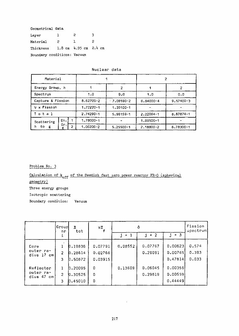
Geometrical data

Layer 1 2 3

Material 2 1 2

Thickness 1.8 cm U.95 cm 2.k cm

Boundary conditions: Vacuum

Nuclear data

MaterialEnergy Group, hSpectrumCapture & Fissionv x FissionT o t a lScatteringh to g

En.Gr.g

12

1

11.0

8.62700-21.72220-12.74290-11.78000-11.00200-2

20.0

< 7.06590-21.30100-15.96159-1

-5.25500-1

2

11.0

6.84000-4-

2.22064-11.99500-12.18800-2

20.0

9.57400-3-

8.87674-1-

8.78300-1

Problem_No_1 3

Calculation of k•eff of the Swedish fast zero power reactor FR-0 (sphericalgeometry)Three energy groupsIsotropie scatteringBoundary condition: Vacuum

Coreouter ra-dius 17 cm

Reflectorouter ra-dius 47 cm

Groupnri

123123

2tot

D. 198360.286140.50872D. 200950. 305250.45010

v2f

0.077910.027660.03915000

ô

j « 1

0.08552

0.13609

j - 2

0.077670.26091

0.060450.29819

j = 3

0.006230.007650.47814

0.003560.005590.44449

Fissionspectrum

0.5740.3930.033

217

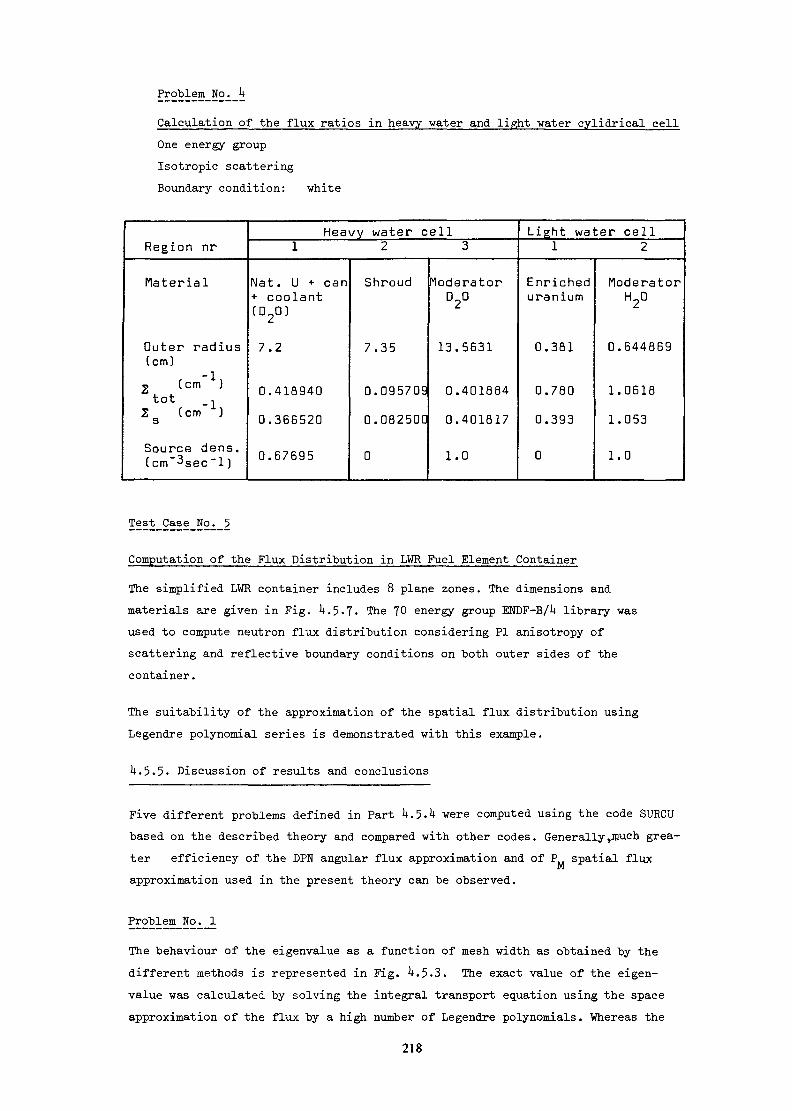
Problem_No_1 ^

Calculation of the flux ratios in heavy water and light water cylidrical cellOne energy groupIsotropie scatteringBoundary condition: white

Region nr

Material

Outer radius(cm)? (cm )2tot 12 (cm )

Source dens.(cm~3sec~l )

Heavy water cell1 2 3

Nat. U + can+ coolant

7.2

0.418940

0.366520

0.67695

Shroud

7.35

0.0957090.082500

0

ModeratorD20

13.5631

0.401884

0.401817

1.0

Light water cell1 2

Enricheduranium

0.381

0.7800.393

0

ModeratorH20

0.644869

1.0618

1.053

1.0

Test Case

Computation of the Flux Distribution in LWR Fuel Element Container

The simplified LWR container includes 8 plane zones. The dimensions andmaterials are given in Fig. U.5.7« The TO energy group ENDF-B/U library wasused to compute neutron flux distribution considering PI anisotropy ofscattering and reflective boundary conditions on both outer sides of thecontainer .

The suitability of the approximation of the spatial flux distribution usingLegendre polynomial series is demonstrated with this example.

U.5.5« Discussion of results and conclusions

Five different problems defined in Part h.5.k were computed using the code SURCUbased on the described theory and compared with other codes. Generally »ffluch grea-ter efficiency of the DPN angular flux approximation and of P spatial fluxMapproximation used in the present theory can be observed.

Problem

The behaviour of the eigenvalue as a function of mesh width as obtained by thedifferent methods is represented in Fig. ^.5-3. The exact value of the eigen-value was calculated by solving the integral transport equation using the spaceapproximation of the flux by a high number of Legendre polynomials. Whereas the

218

collision probability method (CP), ANISN (S ) (ENGLE (1967)), S method (MENNIG(1968)) and the presented method (PN/PM) results vere obtained with one-dimensio-nal calculations, diffusion (CODIFF) (PAEATTE (1971*)) DOIT 3 (S ) (ARKUSZEWSKI(1973)) and Maeder's QPO and QP1 (MAEDER (1975)) results are obtained with two-dimensional calculations taken from (MAEDER (1975))- To simulate the infiniteextension of the slab in the y-direction two mesh intervals with Ay = Ax andreflective boundary conditions were used.

The SURCU results are given by PN/PM where PN means the DPN angular boundaryflux approximation and PM means the spatial approximation of the flux in onemesh.

From Fig. U.5.3 it can be seen that the DPN approximation in the proposed methodconverges very well; better than S approximation. Due to the assumption of theconstant mesh flux, the dependence of the results on the chosen mesh width isvery -strongwiththe DPN/PO approximation of the proposed method as it is alsowith CP, QPO and DOIT 3. The other codes and DPN/P1 approximation in the pro-posed method use the assumption of a linearly varying mesh flux and show there-fore more satisfactory mesh size dependence. The best convergence was reachedwith a P3./P2 approximation in the proposed method. Already 2 meshes lead toa very high accuracy of results.

Convergence to the exact value is not achieved with the transport codes DOIT 3and QP1 (mainly with QPO approximation) due to the low and fixed angularboundary flux approximation as well as with CODIFF due to the diffusion approach.

A very well known property of S theory can be demonstrated from Fig. U.5.3:namely that with increasing number of meshes the increasing S approximationshould be used. Because the proposed theory is itheory, the same property can be observed here.should be used. Because the proposed theory is in many ways close to the S

Problem_No. 2

Also in this two energy groups, three layer problem the DPN angular boundaryflux approximation in SURCU leads to a very good convergence (see Table 4.5.1).A P3 approximation is comparable to that of S , . Only PO spatial flux approxi-mations were used in the SURCU computations.

Problem No._3

In this series of calculations, the k of the fast zero-power reactor FR-0was calculated. Three energy groups were considered. The k „-'s calculated bySURCU, ANISN and DIT are plotted in Fig. k.^.k. Whereas P2/P1 and P3/P2approximation in SURCU leads to accurate results already for few space inter-vals, the DIT and ANISN converge very slowly. High S approximation must beused in ANISN.

219

Problem_No._l( and ka.

The flux ratios $ /$ „ and $ /ft , where $ , $ and i are average fluxes inmi s f m s fmoderator, shroud and fuel, resp. are computed in the heavy water cell usingSURCU, ANISN, DIT and CP method. The results are plotted in Fig. .5.5.

The DPN convergence is much faster than S convergence. The spatial convergenceof the S method is close to that of P2/P1. Whereas P3/P2 converge to the rightresult already for four mesh intervals, the Pl/PO and CP methods require manyintervals .

The values of Ï /$„ ratio of the average flux in moderator and fuel, resp.,m ffor light water cell are shown in Fig. k.5.6.

Because the optical thickness is small the S convergence is very poor. However,SURCU converges very fast, P3/P2 and also P /Pl converge very good in spacealso, whereas the DIT, CP, S and Pl/PO methods converge slowly.

Problem

The LWR fuel element container has originally X-Y geometry. It includes boral

zones, in which the boral is composed of many boral spheres embedded in thealuminium matrix.

In order to consider the double-heterogeneity effect of the grain structureof the boral, the X-Y geometry of the container was simplified into slabgeometry. Then the "overall" flux ditribution in each zone and the "micro"flux distribution in the spheres and in the Al matrix was computed using thespecial version of SURCU, SURCU-DH (STEPANEK (1978)). Using the "micro" fluxdistribution in the boron spheres and the Al -matrix, the boral zone can behomogenized and after condensation of the 70 groups into a small number ofgroups, the computation of X-Y flux distribution can be performed.

In Fig. U.5.7 the "overall" flux distribution computed by SURCU-DH for (N=2,L=l, M=0), (N=2, L=l, M=l) and (W=3, L=l, M=2) is plotted. It is shown, thatalso very irregular flux distributions with fluctuations of several magnitudescan be approximated quite well using Legendre polynomial series.

The energy groups are in the range:

Group 5 : 1.353 MeV i 2.231 MeV25 : 27.700 eV T W. 052 eVh6 : 0.625 eV T 0.780 eV70 : 0.0 eV * 0.005 eV

220

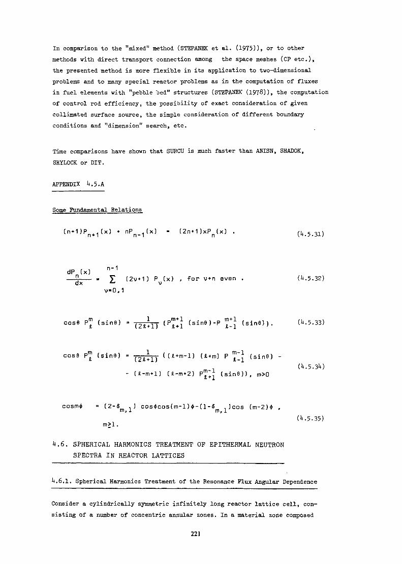
In comparison to the "mixed" method (STEPAHEK et al. (1975)), or to othermethods with direct transport connection among the space meshes (CP etc.),the presented method is more flexible in its application to two-dimensionalproblems and to many special reactor problems as in the computation of fluxesin fuel elements with "pebble bed" structures (STEPANEK (1978)), the computationof control rod efficiency, the possibility of exact consideration of givencollimated surface source, the simple consideration of different boundaryconditions and "dimension" search, etc.

Time comparisons have shown that SUECU is much faster than ANISN, SHADOK,SHYLOCK or DIT.

APPENDIX It. 5. A

Some Fundamental Relations

(2n+1)xPn(x) . (U.5.31)

dP (x) n"1% (2v+1) PV(X) , for v + n even . (U.5-32)

v-0,1

cose P™ (sine) = [2il+l] (Pj*j (sine)-P ™* (sine)). (U.5.33)

cose P™ ( s i n e ) = (2J tin ( U + m - 1 ) U+m) P ™~J ( s i n e ) -.

- ( J l - m + 1 ) ( J l - m + 2 ) P + ( s i n e ) ) , m > o

cosm* = C2-6m ,) cos«cos(m-l )*-( l -6 . )cos ( m - 2 ) * ,m» i m, l(U.5 .35)

4 .6 . SPHERICAL HARMONICS TREATMENT OP EPITHERMAL NEUTRONSPECTRA IN REACTOR LATTICES

U.6.1. Spherical Harmonics Treatment of the Resonance Flux Angular Dependence

Consider a cylindrically symmetric infinitely long reactor lattice cell, con-sisting of a number of concentric annular zones. In a material zone composed

221

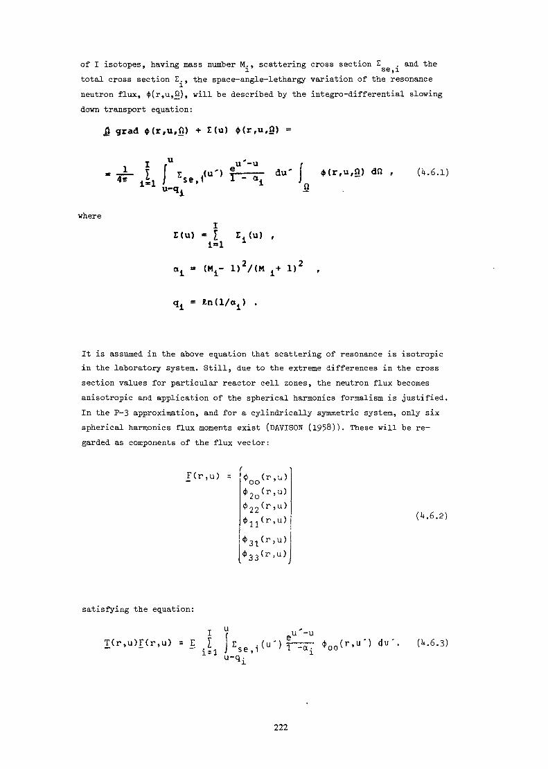
of I isotopes, having mass number M. , scattering cross section £ . and thei se , 1total cross section I., the space-angle-lethargy variation of the resonanceneutron flux, <(>(r,u,J2), will be described by the integro-differential slowingdown transport equation:

ß grad

U-q<

(U.6.1)

whereZ(u)

1=1

*i * (Mi" 1 ) 2 / ( M i+ 1)2 •

It is assumed in the above equation that scattering of resonance is isotropicin the laboratory system. Still, due to the extreme differences in the crosssection values for particular reactor cell zones, the neutron flux becomesanisotropic and application of the spherical harmonics formalism is justified.In the P-3 approximation, and for a cylindrically symmetric system, only sixspherical harmonics flux moments exist (DAVISON (1958)). These will be re-garded as components of the flux vector:

F(r,u) =*2o(r'u)(|>22(r,u)

(U.6.2)

satisfying the equation:

i y u'-uT(r ,u )F ( r ,u ) = E _[ J E g e ^ ( u * ) 3-157 * 0 0 ( r , u ' ) d u ' . (U.6.3)

u-q. '

222

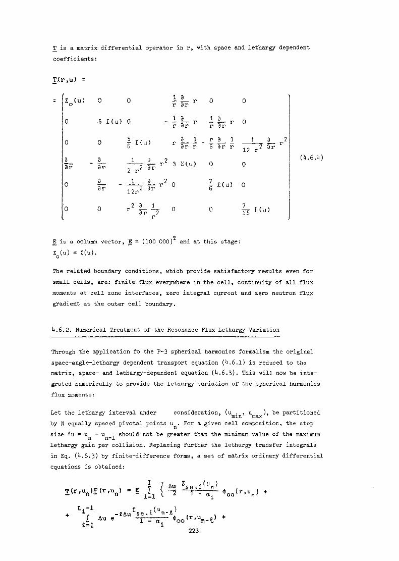
T_ is a matrix differential operator in r, with space and lethargy dependentcoefficients:

T.(r,u) =

Ï0(u)

33r

.5 Hu) 0

Hu)

3_ _1__ 3_ 23r 2 p2 3r T

3 _ l | _ r 2 03r 12p2 3r

Y* z._ .i_ ni r\ -wrr-r f^J

3r 2r

i !_ rr 3r

i L. rr 3r

3 1r 3r r

3 Hu)

0

0

0

r 3r

r 3__ 16 9r r

0

Ï z ( u )b

0

0

0

1 3 r212 r2 3r

0

0

71 5 '

(U.6.U)

]3 is a column vector, 15 = (100 000) and at this stage:ZQ(U) = ï(u).

The related boundary conditions, which provide satisfactory results even forsmall cells, are: finite flux everywhere in the cell, continuity of all fluxmoments at cell zone interfaces, zero integral current and zero neutron fluxgradient at the outer cell boundary.

k.6.2. Numerical Treatment of the Resonance Flux Lethargy Variation

Through the application fo the P-3 spherical harmonics formalism the originalspace-angle-lethargy dependent transport equation (U.6.1) is reduced to thematrix, space- and lethargy-dependent equation (lt.6.3). This will now be inte-grated numerically to provide the lethargy variation of the spherical harmonicsflux moments :

Let the lethargy interval under consideration, (u . ,mm u ), be partitionedmaxby N equally spaced pivotal points u . For a given cell composition, the stepsize AU = u - u .. should not be greater than the minimum value of the maximumn n-1 &

lethargy gain per collision. Replacing further the lethargy transfer integralsin Eq. (U.6.3) by finite-difference forms, a set of matrix ordinary differentialequations is obtained:

T(r,un)F(r,un)

V1l Au e"£=1

Au

223

Ctn = 1,2,...,N; = u + nAu ; umgx « umin + NAu.mgx

L. is the largest integer value of the quotient q./Au ; C. is the differencecorrector of the trapezoidal formula, referring to the i-th isotope.

If the pivotal points u are sufficiently dense, so that the difference correctionnmay be ignored, the system of matrix differential equations (k.6.5) takes alower block triangular form and can be directly solved by forward block sub-stitution. Knowing, or assuming, the space- and lethargy-flux variation at andbelow u . , the spatial distribution of the resonance flux at u > u . canmin n minbe determined by successive solution of the nonhomogeneous ordinary differentialequations :

T" is a matrix differential operator given by Eq. (U.6.U), but with modified I :oI Z • ( u }

T fil 1 - Vf \ Au r s e » 1 * P'on' * E(un) ~ T~ i- ~ï———— • ( .6.7)i=l x ' °4

U.6.3. Approximate Analytical Solution for the Space Variation of Resonance Flux

In each step of numerical integration over lethargy a boundary value problemhas to be solved for a nonhomogeneous system of ordinary differential equations(h.6.1). In order to avoid difficulties associated with standard numericalmethods, which could make the whole procedure impracticable, the attentionis turned to a combination of numerical and analytical techniques.

To initiate the numerical integration over lethargy suppose that below and atu . the neutron flux is spatially flat in each cell zone. Then, at the firstminpivotal point u , Eq. (U.6.6) takes a simple form:

T'(r,u..)F(r,u.,) = E C. , (U.6.8)— 1 — J — O

224

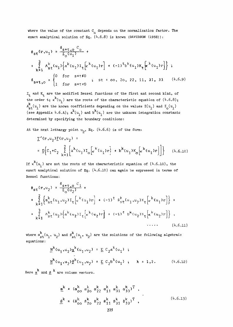
where the value of the constant C depends on the normalization factor. Theoexact analytical solution of Eq. (4.6.8) is known (DAVIDSON (1958)):

A C, , . S + t,O 'O*st (r'ul ) = l (ÙJ—— +

3

kI Agt(u1){ak(u1)It[<k(u1)r] + (-1 )tbk(u1)Kt \K u^r] J ;

[O for s+ttQS . - { ; st = oo, 2o, 22, 11, 31, 33 (4.6.9)

S"l"t'° [l for s+t=0

I and K are the modified Bessel functions of the first and second kind, ofkthe order t; K (u ) are the roots of the characteristic equation of (4.6.8);

A .(u ) are the known coefficients depending on the values £(u ) and £ (u )s t l l o iK K(see Appendix 4.6.A); a (u ) and b (u ) are the unknown integration constants

determined by specifying the boundary conditions:

At the next lethargy point u?, Eq. (4.6.6) is of the form:

T'(r,u2)F(r,u2) =

(4.6.10)

If K (u ) are not the roots of the characteristic equation of (4.6.10), theexact analytical solution of Eq. (4.6.10) can again be expressed in terms ofBessel functions:

ô _ C,

j, Ast(V{ak(Vrt[KK("2H * (-a)t bk(u2)Kt[Kk(u2)r]} ,3\

k:• • • • • (4.6.11)

k kwhere a (u , u ) and $ .(.(u-,» U0 are e solutions of the following algebraicSt 1 c. St l c.equations :

Nk(u1,u2)o.k(u1,u2) = E C2ak(u1) -,

Nk(u1,u,)ßk(u1,u9) = E C9bk(Ul) ; k = 1,2. (U.6.12)"" J./ — J./ — c. 1

k kHere a and ß are column vectors.

k = («oo «20 «22 «Ï1 «5l «33)T 'k _ k Rk k k Rk k .T (4-6.13)

- (0oo ß2o ß22 ßll 331 ß33} '225

and BT(u , u ) is the matrix:

E0(u2) 0

5 E(u2) 0 -ic

3E(u2) 0

\

<^(u1) 0

(U.6.1U)

It is not possible to continue the numerical integration over lethargy in theabove manner and the exact analytical solution of Eq.. (U.6.10), which in thegeneral case can not be expressed in the form (U.6.11), will only be used hereto introduce and examine a new approximate procedure based on a convenient com-bination of numerical and analytical treatment.

Let each cell zone be divided into a number of subzones and suppose that in asubzone z, having outer radius r , the right hand side of Eq. (U.6.10) is

Z

approximated by its volume averaged value:

T'(r/u2)fz(r,u2) » F YZ(UI> for r

Vul} = Cl +

r (U.6.15)

r2-J (U.6.16)For each of the subzones, the approximate analytical solution of Eq. (U.6.10)is then:

'-v •

(U.6.17)

k kThe integration constants a and b are allowed to have different values inZ Zeach subzone in order to provide continuous flux moments everywhere in the cell.They are determined by the interface conditions:

226

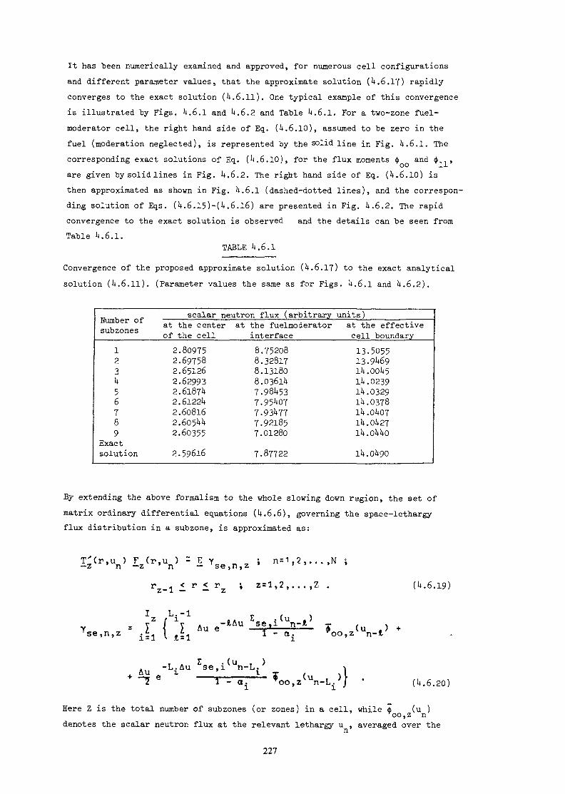
It has been numerically examined and approved, for numerous cell configurationsand different parameter values, that the approximate solution (U.6.17) rapidlyconverges to the exact solution (U.6.11). One typical example of this convergenceis illustrated by Figs. U.6.1 and k.6.2 and Table U.6.1. For a two-zone fuel-moderator cell, the right hand side of Eq. ( .6.10), assumed to be zero in thefuel (moderation neglected), is represented by the solid line in Fig. U.6.1. Thecorresponding exact solutions of Eq. (It.6.10), for the flux moments <£ and <$>,-,,

are given bysolidlines in Fig. U.6.2. The right hand side of Eq. (U.6.10) isthen approximated as shown in Fig. U.6.1 (dashed-dotted lines), and the correspon-ding solution of Eqs. (I*.6.15)-( .6.l6) are presented in Fig. h.6.2. The rapidconvergence to the exact solution is observed and the details can be seen fromTable U.6.1.

TABLE U.6.1Convergence of the proposed approximate solution (U.6.17) to the exact analyticalsolution (U.6.11). (Parameter values the same as for Figs. U.6.1 and U.6.2).

Number ofsub zones

123k56789

Exactsolution

scalar neutron flux (arbitrary units)at the centerof the cell2.809752.697582.651262.629932.61872.61221+2.6o8l62.6052.603552.59616

at the fuelmoderatorinterface8.752088.328178.131808.0361U7.98 537.95 07T.93VT77.921857.012807.87722

at the effectivecell boundary13.505513.9U69l^.OOi+5lU.02391U.03291 .0378ik.QkQJ1Î+.OU27Ik.QhkO

ik.ohgo

By extending the above formalism to the whole slowing down region, the set ofmatrix ordinary differential equations (h.6,6), governing the space-lethargyflux distribution in a subzone, is approximated as:

1 r,"— Z t. 6. 19)

. -LjAu Ese,i(un-Li)(U.6.20)

Here Z is the total number of subzones (or zones) in a cell, while ï (u )oo,z ndenotes the scalar neutron flux at the relevant lethargy u , averaged over the

227

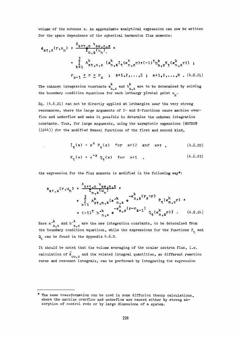
volume of the subzone z. An approximate analytical expression can now be writtenfor the space dependence of the spherical harmonics flux moments:

A (n n ï - s+t,o Yse,n,z(r - —

r, . < r < r, i z=l,2,...,Z ; n=l,2,...,N . {U. 6. 2l)Z"" l "" "" Z

k kThe unknown integration constants a and b are to be determined by solvingn,z n,zthe boundary condition equations for each lethargy pivotal point u .

Eq. (U.6.21) can not be directly applied at lethargies near the very strongresonances, where the large arguments of I- and K-functions cause machine over-flow and underflow and make it possible to determine the unknown integrationconstants. Thus, for large arguments, using the asymptotic expansions (WATSON

for the modified Bessel functions of the first and second kind,

I t (x) = ex P (x) for x>12 and x>t , (U.6 .22)

K t (x ) = e~x Q t ( x ) for x>l , (U.6.23)

the expression for the flux moments is modified in the following way*:

b'n,z e"Kn>Z r"T'Z"1 Qt(<n,zr)}k kHere a' and b" are the new integration constants, to be determined fromn,z n,z

the boundary condition equations, while the expressions for the functions P andQ can be found in the Appendix U.6.B.

It should be noted that the volume averaging of the scalar neutron flux, i.e.calculation of $ and the related integral quantities, as different reacticrates and resonant integrals, can be performed by integrating the expression

* The same transformation can be used in some diffusion theory calculations,where the machine overflow and underflow are caused either by strong ab-sorption of control rods or by large dimensions of a system.

228

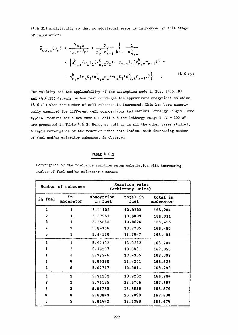
(k.6.2l) analytically so that no additional error is introduced at this stageof calculation:

' n , zz A 2 P lTTT + ~"7—5— i —JT~" rz-rll k=1 <S

- 'VlV'n.z'Vl» -

(U.6.25)

The validity and the applicability of the assumption made in Eqs. (U.6.19)and (U.6.29) depends on how fast converges the approximate analytical solution(U.6.21) when the number of cell subzones is increased. This has been numeri-cally examined for different cell compositions and various lethargy ranges. Sometypical results for a two-zone U-C cell a d the lethargy range 1 eV - 100 eVare presented in Table U.6.2. Here, as well as in all the other cases studied,a rapid convergence of the reaction rates calculation, with increasing numberof fuel and/or moderator subzones, is observed.

TABLE 4.6.2

Convergence of the resonance reaction rates calculation with increasingnumber of fuel and/or moderator subzones

Number

in fuel123451111112345

of sub zone sin

moderator11111123i»5123H5

Reaction rates(arbitrary units)

absorptionin fuel5.911025.879675.858655.847665.8»H205.911025.791075.725U65.693905.677175.911025.761355.677305.636495.61442

total infuel

13.923213.849913,802613.778513.764713.923213.646113.493513.420113.381113.923213.576613.382613.289013.2388

total inmoderator166.204166.331166.415166.460166.485166.204167.855168.392168.623168.743166.204167.967168.570168.834168.974

229

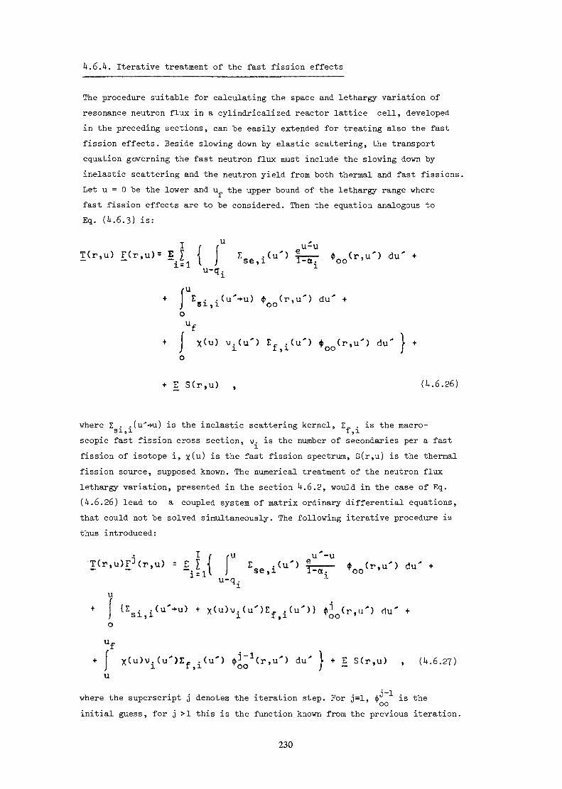
k. 6. k. Iterative treatment of the fast fission effects

The procedure suitable for calculating the space and lethargy variation ofresonance neutron flux in a cylindricalized reactor lattice cell, developedin the preceding sections, can be easily extended for treating also the fastfission effects. Beside slowing down by elastic scattering, the transportequation governing the fast neutron flux must include the slowing down byinelastic scattering and the neutron yield from both thermal and fast fissions.Let u = 0 be the lower and u the upper bound of the lethargy range wherefast fission effects are to be considered. Then the equation analogous toEq. (U.6.3) is:

y U >•

T(r,u) F(r,u)= E [ ( f z (u') |1^ * (r,u') du' +£_^ l J se,i iu-q.

e. . 4» (r,u') du51,1 OO* rouf+ J x<u> (u') Zf>i<u') *00<r,u') du' } +

o

+ E S(r,u) , (U.6.26)

where £ . . (U'-HI) is the inelastic scattering kernel, £ . is the macro-S 1 5 1 I j 1

scopic fast fission cross section, v. is the number of secondaries per a fastfission of isotope i, x(u) is "the fast fission spectrum, S(r,u) is the thermalfission source, supposed known. The numerical treatment of the neutron fluxlethargy variation, presented in the section U.6.2, would in the case of Eq.(4.6.26) lead to a coupled system of matrix ordinary differential equations,that could not be solved simultaneously. The following iterative procedure isthus introduced:

T(r,u)Fj(r,u) = E I { [ z (u') fl— * (r,u') du' +;-l\ J se,i I~ai1 °°u-q.

u+ {E . .(u'-»-u) + x(u)v.(u')E,. .(u')} d»^ (r,u') du' +j si,i i r,i oo 'o

u+u

If x<u)v.(u')E,r .(u') ( " (r.u') du' i + E S(r,u) , (U.6.27)j i r j i oo j —

where the superscript j denotes the iteration step. For j=l, <)> is theinitial guess, for j >1 this is the function known from the previous iteration.

230

Convergence of the above iteration scheme is very good. The total neutronbalance condition can serve as the criterion for the completion of theiteration procedure: the total number of neutrons absorbed in the lethargyregion considered, or scattered out of this region, must equal, to the desiredaccuracy, the total number of neutrons born in thermal and fast fissions.

Further treatment of Eq.. (i*.6.27) can be exactly the same as the one proposedin the sections 2. and 3. and the expression for the neutron flux moments,analogous to Eq.. (U.6.21), i.e. (U.6.2l|), is derived. This will now be givenin a condensed matrix form:

,3I A4 ——J » y «4 ——— ff ,o,n,z; z=l,2,...,Z ; n=l,2,..,,N

Here 0 _ ( r ) are row vectors:""""II y Z

0 .(r) = (o1 , a2 , a3 ,)—n, l —n, l —n, l —n, l

e2 s3

(It.6.28)

(U.6.29)

whose elements are the six-order column vectors

ka =— n,z Akoo , n , z

Ak2o,n,z

.kA 2 2 , n , z

V-AA l l ,n ,z\fAn31,n,zAk

33, n, z

ko n,

^ / ko n,

B (tck

JçB l ( K n,

1-B l ( l Cn,B 3 ( K n,

r)

z

z

zr)

zr)

zr) .

z = l,2,, . . ,Z ,k=l,2,3 , (U.6.30)

flk --n,z ' Akoo,n,z

Ak2o,n , z

Ak22, n, z

-Ak

-Ak *n 'ZA31,n,z

-AkA 33,n ,z

fc '

yo n,z

kD2 n,z r

k

Dl<zr>D3 ( ( fn,z r ) .

, z = 2 , 3 , .k = l , 2 , 3

(U.6.31)

231

Functions B and D &re related to the modified Bessel functions of thet "t

first and second kind and are defined as:

-< (r -r)Ptc-.; P,for n,z z-1—12

for ** r >12 (U.6.32)D ) <£ J

for K* r -,<!n,z z-1—

'' V"n,zr) for Kn,zrz-l>:l (U.6.33)

In Eq.. (U.6.28), xj is a column vector of the order (3x1) for z=l and of~n,zthe order (6xl) for z=l,2,...,Z, whose elements are the unknown integrationconstants. The ojuantity y is the value of the lethargy transfer integraln^ zand outer neutron source calculated in the iteration step 1, for the lethargypoint u and the subzone z:n

se,n,z .si,n,z f,n,z n,z (U.6.3U)

where Y > Y • and y. represent the yield of lethargy use,n,z 'si,n,z f,n,z * J ^ nneutrons from elastic and inelastic collisions below u , and from fastnfissions, respectively, while S is the outer source of the lethargy un g z nneutrons, averaged over the volume of the subzone z.

To determine y , extending the procedure presented in the section U.6.2,n,zthe following recurrence relations have been devived (the subscript z, re-ferring to a cell subzone, being omitted for brevity):

-L. AuZse,i(VV

si ,nsi

232

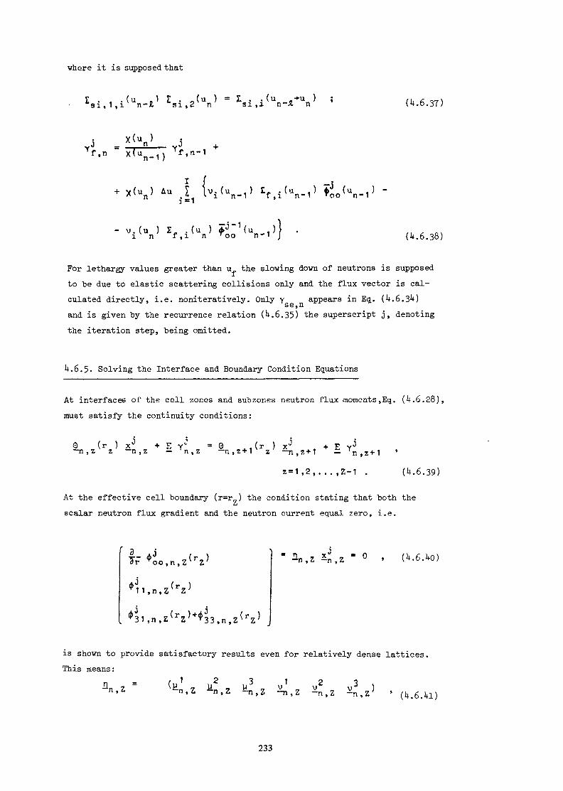
where it is supposed that

t.6.37)

f,n

X(un)

Tf,n-1

(4.6.38)

For lethargy values greater than u the slowing down of neutrons is supposedto be due to elastic scattering collisions only and the flux vector is cal-culated directly, i.e. noniteratively. Only y appears in Eg.. (4.6.3*0s G y nand is given by the recurrence relation (4.6.35) the superscript j, denotingthe iteration step, being omitted.

4.6.5- Solving the Interface and Boundary Condition Equations

At interfaces of the cell zones and subzones neutron flux moments,Eq. (4.6.28),must satisfy the continuity conditions:

Q (r ) x1-1 + E YJ =9 AT ) xj + E Y^-n,z z -n,z - 'n,z -n,z+1 z -n,z+1 — n,z+1 'a-1,2,...,Z-1 . (4.6.39)

At the effective cell boundary (r=r ) the condition stating that both thescalar neutron flux gradient and the neutron current equal zero, i.e.

° •

is shown to provide satisfactory results even for relatively dense lattices.This means :

l 1 2 3 1 2 3n'Z «»Z Mn.Z En,Z TI , Z ^n, Z ^n, Z} ' (U.6.1*l)

233

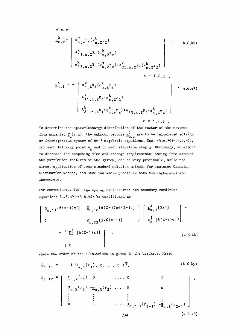
wherek

(U.6.U2)

1,2,3 ,

t.6.U3)

k = 1,2,3 .To determine the space-lethargy distribution of the vector of the neutronflux moments, F (r,u), the unknown vectors x are to be calculated solving—z —n,zan inhomogeneous system of 6z-3 algebraic equations, Eqs. (U.6.39)-( .6.Uo),for each lethargy point u and in each iteration step j. Obviously, an effortnto decrease the computing time and storage requirements, taking into accountthe particular features of the system, can be very profitable, while thedirect application of some standard solution method, for instance Gaussianelimination method, can make the whole procedure both too cumbersome andinaccurate.

For convenience, let the system of interface and boundary conditionequations (U.6.39)-(U.6.Uo) be partitioned as:

& „(6(2-0x3) « 15(6(z-Ox6(z-O]n j i i n 9 i &

. 0 r3 (6(z-Oxi)

—n (6(z-Oxij (U.6.UU)

where the order of the submatrices is given in the brackets. Here:

--n , 1 1

12

, 0,..., 0 ) x,

i .... 0

'. ,(r„) .... 0

(U.6.U5)

0

0

234 (U.6.U6)

8 n,22 - <° o ... o nn?z) , (U.6.UT)

* ° - ( . *..., « , (U.6.U8)

^ -X7,2 ,i - z'Ctii • (h'6'hg}Eliminating XJ from Eq.. (k.6.kk) one obtains:—n

an , ( * - , > ] I An z ECîU - liil ^ (U.6 .50)n > z = 1 n ' Z o ,n ,2+l

where X are the block elements of the matrix A ,—n,z — n

and can be easily obtained by direct back substitution from the system

î 5n,12 = n,22 . (1*.6.52)

4,Z-1 = ' n.Z .Z Z-l , (U.6.53)— 1

*n,z " \,z+l n,z+l(rz+l) .z+l z , (U.6.5U)z = Z-2S Z-3, ... 2, 1 .

Knowing xj , , xj for z l is directly obtainable from Eq. (k.6.39):~n,l — n,zj = (6 (r Jf1 0 .(r J xj . +n,z — n,z z-1 — n,z-l z-1 — n,z-l

( » ' 1 s '^ - 8^-' • ""6-55)

xj— n,

o,n,z-l o,n,z

z = 2, 3, ..., Z.

Eqs. (U. 6. 50) and (U. 6. 55) can be further simplified:Z-1 -y^r

z = 2, 3, ..., Z , C*-6.57)

where the vectors E and ç and the matrix il do not change in theHjZ n,z *TI,Zcourse of iterations:

In, z = ( ,1 Sn.iî)) -1 in>2 I , z = l,2,...,Z-l ,(»«.6.58)

235

n,z = ten.z z-l '1 £ ' 2 = 1,2,....Z , (4.6.59)

Substituting Eqs. (4.6.56)-(4.6.57) into Eq. (4.6.28) the spatial distributionof the vector of spherical harmonics flux moments is obtained.

Compared to standard computational methods (ISMCSON and KELLER (1966)),which can be applied to solve the system of interface and boundary conditionequations (4.6.39)-(4.6.1*0), the above procedure is advantageous. It requiresthe minimum number of operations, since it takes into account all zero elementson both the right and the left sides of the system and it avoids repeated cal-culations in the course of iterations. Better accuracy can also be expected,since only the solution of algebraic systems of order not greater than sixis required.

4.6.6. Results and discussion

In the previous sections the complete algorithm is presented for calculatingthe space—lethargy distribution of the spherical harmonics flux moments, fora given reactor lattice cell and in a given epithermal lethargy range (MATAUSEK(1972),(1978)). This will now be summarized according to the sequence neededfor numerical calculations.

For a given cylindrical reactor lattice cell and a given lethargy interval(u . . u ) the cell subzones and the lethargy pivotal points are to benun' max ^ * *determined taking into account the slowing down properties of the reactormaterials involved. For lethargy values where the fast fission effects areto be considered, i.e. for u . < u < u ,, the calculation is performed ite-' nan- - f' *ratively. As the initial guess the spatially flat flux, having the samelethargy distribution as the last fission neutrons, can be supposed. Matricesand vectors which do not change in the course of iterations are calculatedfirst, for all lethargy points u„> u > u . and for all zones and subzones,017 f - n - minz=l,2,...Z. These are quantities Ç , ç and iji , defined by Eqs.~"'Ti ) z *~n9 z ~TL y z(4.6.58)-(4.6.6o), which incorporate Eqs. (4.6.29)-(4.6.33), (4.6.4l)-(4.6.43),(4.6.53) and (4.6.54). Iterative procedure consist of repeated calculationsof Y and F"5 (r) according to Eqs. (4.6.34)-(4.6.38), (4.6.56)-(4.6.57)n 3 z n j zand (4.6.28).

After the calculation for u < u„ is completed, and if u > u_, nonitera-- f max ftive calculation is performed for the lethargy points u > u > u„ ,max - n fusing the results of the iterative treatment as the initial condition inlethargy. Here Ç , ç and ii are not to be stored in the memory°* -n,z -n,z zn,zculated successively, together with the quantities v , x and F (r).n,z -n,z -n,z

236

The same noniterative procedure is immediately applied if u . > u_. It canmin rthen be supposed that for u < u . the neutron flux is spatially flat and- mmlethargy independent.

According to the above algorithm a FORTRAN IV program has been written forthe CDC 3600 computer (MATAUSEK (1975)). The space and lethargy distributionof epithermal neutrons in a cylindricised reactor lattice cell, and therelated integral quantities, can be determined as detailed as the neutroncross sections are known for the materials considered. Some typical resultswill now be presented, obtained using the KEDAK nuclear data (LANGER et al.(1968)).

Fig. k.6.3 is an illustration of the lethargy variation of the resonanceneutron flux at the center of the fuel element, at the fuel-moderator inter-face and at the outer boundary (the curves are deonoted by 1,2 and 3» respecti-vely) of a two-zone enriched uranium - H.O cell. The figure covers the range100 eV - 10 eV, where the strong variations of the flux are caused by largenumber of unresolved U-235 resonances and also by the strong resolved re-sonances of U-238. The arrows in the figure point the positions of these"giant" U-238 resonances.

In Fig. k.6.k the energy distribution of the average flux in the fuel andmoderator of a U - C cell, through the 6.7 eV resonance of U-238, obtainedby the proposed method supposing the 1/v absorption in U-235 (curves 1),or taking into account the detailed variation of U-235 cross sections (curves 2),is compared with the results of Lewis and Adler (1968) (curves 3). The agree-ment can be considered satisfactory.* For the energy -values denoted in Fig.k.6.k by a - d, the radial variation of the flux is given in Fig. U.6.5-

It can be noticed here that at resonance energies polynomial representation,used with the integral transport theory treatment of Refs. (LEWIS andADLER (1968)), and also (KIER et al. (1967)), is very unconvenient for thespatial variation of the neutron flux in the fuel.

The results presented here, as well as the other results showthat the proposed procedure is on efficient way to calculate the detailedspatial and lethargy distribution of epithermal neutrons in a multizonecylindrically symmetric reactor lattice cell. The computing time is relati-vely short, what makes the proposed procedure suitable for practicalapplications. In the present form the procedure can treat only isotropic

The linear parts of curves 1 and 2 between 7-5 eV and 10 eV are due to linearinterpolation in the tables of the cross section values. Parabolic interpola-tion, suggested in Ref. (LANGER et al. (1968)), for resonance wings, couldnot be performed since it led to oscilatory results.

237

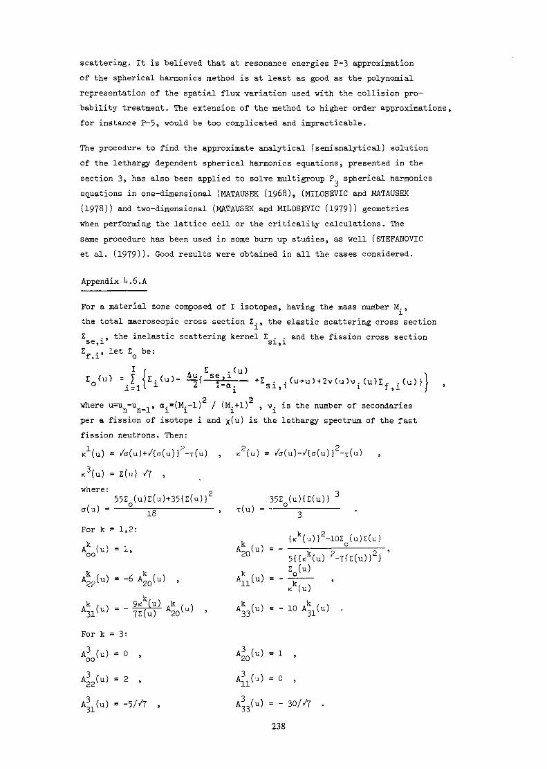
scattering. It is believed that at resonance energies P-3 approximationof the spherical harmonics method is at least as good as the polynomialrepresentation of the spatial flux variation used with the collision pro-bability treatment. The extension of the method to higher order approximations,for instance P-5» would be too complicated and impracticable.

The procedure to find the approximate analytical (semianalytical) solutionof the lethargy dependent spherical harmonics equations, presented in thesection 3, has also been applied to solve multigroup P_ spherical harmonicsequations in one-dimensional (MATAUSEK (1968), (MILOSEVIC and MATAUSEK(1978)) and two-dimensional (MATAUSEK and MILOSEVIC (1979)) geometrieswhen performing the lattice cell or the criticality calculations. Thesame procedure has been used in some burn up studies, as well (STEFANOVICet al. (1979)). Good results were obtained in all the cases considered.

Appendix U.6.A

For a material zone composed of I isotopes, having the mass number M. ,the total macroscopic cross section E., the elastic scattering cross section£ . , the inelastic scattering kernel I . . and the fission cross sectionse,i °r > l e t l b e :

r0<u) =2 2where u=u -u , ct.=(M.-l) / (M.+l) , v. is the number of secondaries

per a fission of isotope i and x(u) is the lethargy spectrum of the fastfission neutrons. Then:K-M » /o(u)+/{a(u)}2-r(u) , <2(u) = /a(u)-/{a(u)}2-T(u) ,

K3(u) = Z(u) /? ,where: „ -,

552 (u)z(u)+35{ï(u)r 35i * O ____________________ / Na(u) = ————— ————————— , T(U) =

For k = 1,2:k k {K (u)} -10£o(u)Z(u)A (u) = 1, Aor/u) = ~ ——— \r ——— 5 —————— 9 —20 5({<k(u) 2-7(l(u)}2}

r(u)

A* (u) = - 10 A* (u) .

For k = 3:

Aoo(u) = ° ' 4>(U) =

= 2 , A(u) = 0 ,

= -5//T , A 3(u) = - 30//7 .

238

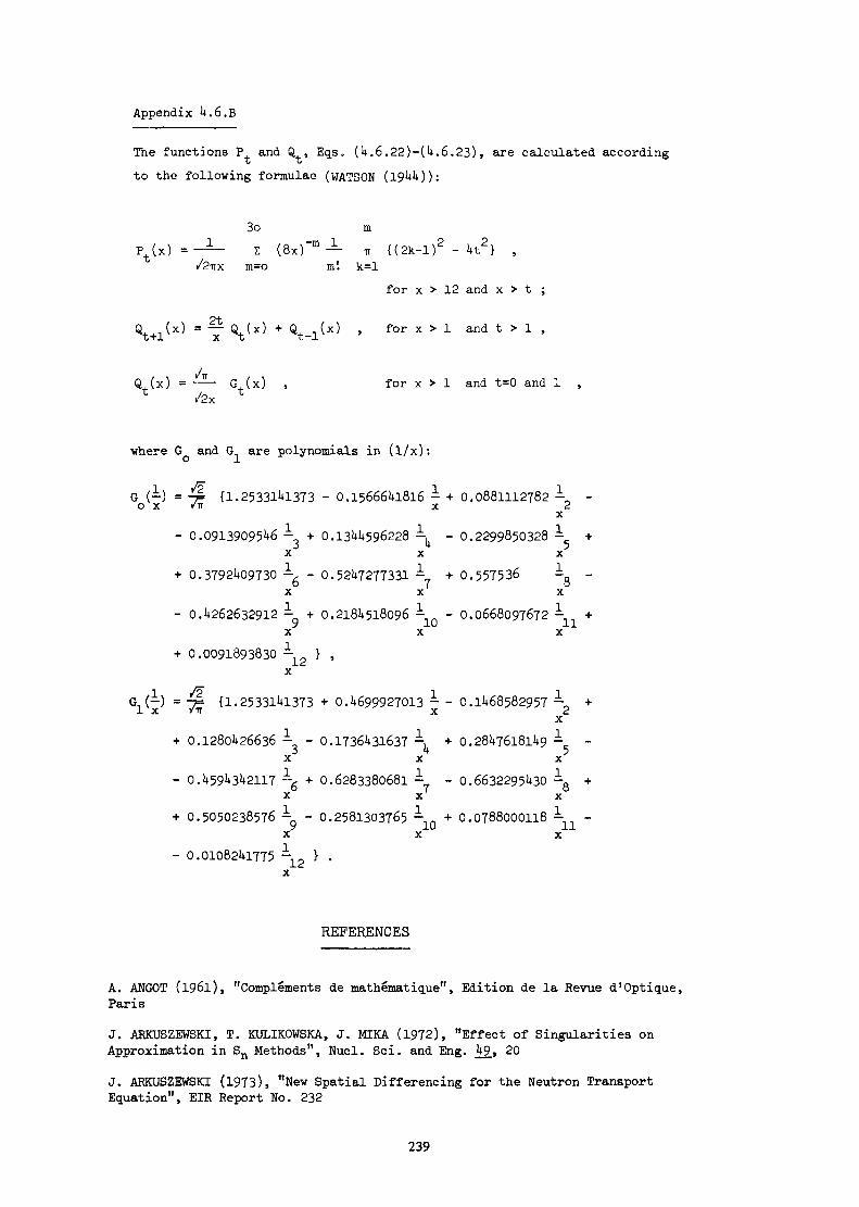
Appendix U.6.B

The functions P and Q , Eqs. (l+.6.22)-(l+.6.23), are calculated accordingt t

to the following formulae (WATSON (19!*!*)):

3o mPt(x)=-^- S (8x)"m— TT {(2k-l)2 - Ht2} ,

/2irx m=o ml k=lfor x > 12 and x > t ;

O4-

Vl(x) = T Qt(x) + Vl(x) ' for x > 1 and t > 1 ,

Q, (x) = -—— G (x) , for x > 1 and t=0 and 1 ,* /2x t

where G and G are polynomials in (l/x):

G (!) = -p (1.253311*1373 - 0.156661*1816 - + 0.0881112782 - -x

- 0.091390951*6 - + 0.131+1*596228 -^ - 0.2299850328 ! +X X X

-f 0.37921*09730 -, - 0.521*7277331 -_ + 0.557536 ! -D f 0

X X X

- 0.1*262632912 - + 0.2181+518096 - - 0.0668097672 - +X X X

+ 0.0091893830 -12 } ,X

G (!) = XI {1.253311+1373 + 0.1*699927013 - - 0.11+68582957 ~0 +JL X * n X f—x

+ 0.12801*26636 - - 0.17361*31637 \ + 0.281+761811+9 ! -X X X

- 0.1+591+31*2117 -s + 0.6283380681 !, - 0.66322951*30 -Q +O 7 0

X X X

+ 0.5050238576 - - 0.2581303765 ~10 + 0.0788000118 ! -X X X

- 0.010621+1775 -12 } .X

REFERENCES

A. AHGOT (I96l), "Compléments de mathématique", Edition de la Revue d'Optique,ParisJ. ARKUSZEWSKI, T. KULIKOWSKA, J. MIKA (1972), "Effect of Singularities onApproximation in Sn Methods", Nucl. Sei. and Eng. 4£, 20

J. ARKUSZEWSKI (1973), "New Spatial Differencing for the Neutron TransportEquation", EIR Report No. 232

239

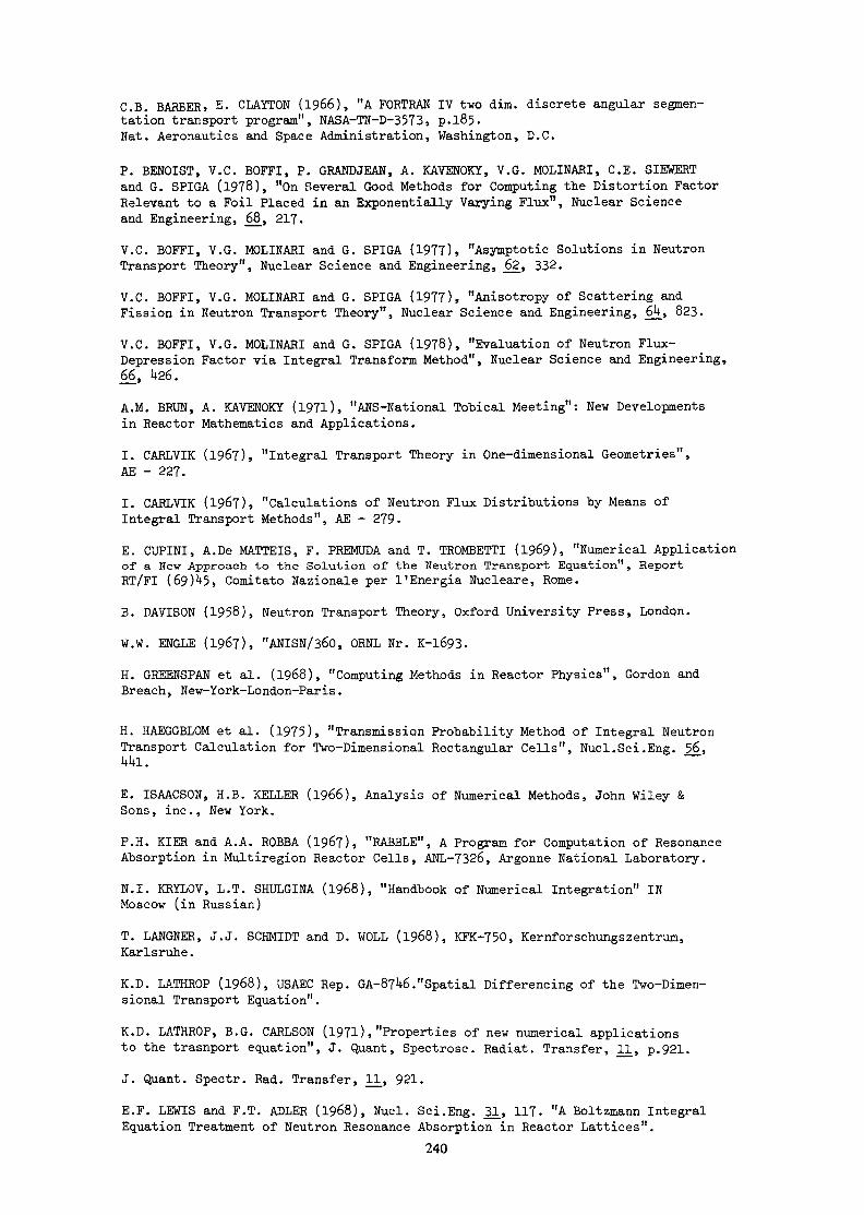
C.B. BARBER» E. CLAYTON (1966), "A FORTRAN IV two dim. discrete angular segmen-tation transport program", NASA-TN-D-3573, p.185.Nat. Aeronautics and Space Administration, Washington, D.C.

P. BENOIST, V.C. BOFFI, P. GRANDJEAN, A. KAVSNOKY, V.G. MOLINARI, C.E. SIEWERTand G. SPIGA (1978), "On Several Good Methods for Computing the Distortion FactorRelevant to a Foil Placed in an Exponentially Varying Flux", Nuclear Scienceand Engineering, 68, 217.V.C. BOFFI, V.G. MOLINARI and G. SPIGA (1977), "Asymptotic Solutions in NeutronTransport Theory", Nuclear Science and Engineering, 62, 332.

V.C. BOFFI, V.G. MOLINARI and G. SPIGA (1977), "Anisotropy of Scattering andFission in Neutron Transport Theory", Nuclear Science and Engineering, 6k, 823.

V.C. BOFFI, V.G. MOLINARI and G. SPIGA (1978), "Evaluation of Neutron Flux-Depression Factor via Integral Transform Method", Nuclear Science and Engineering,66, U26.A.M. BRUN, A. KAVENOKY (1971), "ANS-National Tobical Meeting": New Developmentsin Reactor Mathematics and Applications.I. CARLVIK (1967), "Integral Transport Theory in One-dimensional Geometries",AE - 227.I. CARLVIK (1967), "Calculations of Neutron Flux Distributions by Means ofIntegral Transport Methods", AE - 279.E. CUPINI, A.De MATTEIS, F. PREMUDA and T. TROMBETTI (1969), "Numerical Applicationof a New Approach to the Solution of the Neutron Transport Equation", ReportRT/FI (69) 5, Comitato Nazionale per 1'Energia Nucleare, Rome.B. DAVISON (1958), Neutron Transport Theory, Oxford University Press, London.

W.W. ENGLE (1967), "ANISN/360, ORNL Nr. K-1693.

H. GREENSPAN et al. (1968), "Computing Methods in Reactor Physics", Gordon andBreach, New-York-London-Paris.

H. HAEGGBLOM et al. (1975), "Transmission Probability Method of Integral NeutronTransport Calculation for Two-Dimensional Rectangular Cells", Nucl.Sci.Eng. 56,UUl.

E. ISAACSON, H.B. KELLER (1966), Analysis of Numerical Methods, John Wiley &Sons, inc., New York.

P.H. KIER and A.A. ROBBA (1967), "RABBLE", A Program for Computation of ResonanceAbsorption in Multiregion Reactor Cells, ANL-7326, Argonne National Laboratory.

N.I. KRYLOV, L.T. SHULGINA (1968), "Handbook of Numerical Integration" INMoscow (in Russian)

T. LANGNER, J.J. SCHMIDT and D. WOLL (1968), KFK-750, Kernforschungszentrum,Karlsruhe.

K.D. LATHROP (1968), USAEC Rep. GA-87U6."Spatial Differencing of the Two-Dimen-sional Transport Equation".

K.D. LATHROP, E.G. CARLSON (1971),"Properties of new numerical applicationsto the trasnport equation", J. Quant, Spectrosc. Radiât. Transfer, 11, p.921.

J. Quant. Spectr. Rad. Transfer, 11, 921.

E.F. LEWIS and F.T. ADLER (1968), Nucl. Sei.Eng. 31, 117. "A Boltzmann IntegralEquation Treatment of Neutron Resonance Absorption in Reactor Lattices".

240

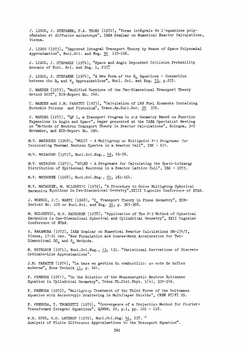
J. LIGOU, J. STEPANEK, P.A. THOMI (1970), "Forme intégrale de 1'equations poly-nômiales et diffusion anisotrope", IAEA Seminar on Numerical Reactor Calculations,Vienna.J. LIGOU (1973), "Improved Integral Transport Theory by Means of Space PolynomialApproximation", Nucl.Sci. and Eng. J>0_ 135-1 6.

J. LIGOU, J. STEPANEK (197*0, "Space and Angle Dependent Collision ProbabilityAnnuals of Nucl. Sei. and Eng. l, 233"J. LIGOU, J. STEPANEK (197*0, "A New Form of the Bn Equations - Connectionbetween the Bn and Pn Approximations", Nucl. Sei. and Eng. 53, p.255-C. MAEDER (1973), "Modified Versions of the Two-Dimensional Transport TheoryMethod DOIT", EIR-Report No. 2*K).

C. MAEDER and J.M. PARATTE (1975), "Calculation of LWR Fuel Elements ContainingBurnuble Poisons and Plutonium", Trans.Am.Nucl.Soc. 20 359«C. MAEDER (1975), "QP 1, a Transport Program in x-y Geometry Based on FunctionExpansions in Angle and Space", Paper presented at the IAEA Specialist Meetingon "Methods of Neutron Transport Theory in Reactor Calculations", Bologna, 3—5November, and EIR-Report No. 290.

M.V. MATAUSEK (i960), "MULTI - A Multigroup or Multipoint, P-3 Programme forCalculating Thermal Neutron Spectra in a Reactor Cell", IBK - 6^h.

M.V. MATAUSEK (1972), Nucl.Sei.Eng., U£, 9-58.

M.V. MATAUSEK (1975), "SPLET - A Programme for Calculating the Space-LethargyDistribution of Epithermal Neutrons in a Reactor Lattice Cell", IBK - 1055-

M.V. MATAUSEK (1968), Nucl.Sci.Eng., 65., l6l-l6*t.

M.V. MATAUSEK, M. MILOSEVIC (1979), "A Procedure to Solve Multigroup SphericalHarmonics Equations in Two-Dimensional Geometry",XXIII Yugoslav Conference of ETAN.

J. MENNIG, J.T. MARTI (1968), "S^ Transport Theory in Plane Geometry", EIR-Bericht Nr. 105 or Nucl.Sci. and°°Eng. 31, p. 365-368.

M. MILOSEVIC, M.V. MATAUSEK (1978), "Application of The P-3 Method of SphericalHarmonics in One-Dimensional Spherical and Cylindrical Geometry", XXII YugoslavConference of ETAN.

S. NAKAMURA (1972), IAEA Seminar on Numerical Reactor Calculations SM-15H/7,Vienna, 17-21 Jan. "New Formulation and Coarse-Mesh Acceleration for Two-Dimensional DSn and Pn Methods.

M. NATELSON (1971), Nucl.Sci.Eng., *t3, 131. "Variational Derivations of DiscreteOrdinate-Line Approximations".

J.M. PARATTE (197*0, "La base en gestion du combustible: un code de boîtesmoderne", Neue Technik 11, p. U6l.

F. PREMUDA (1971), "On the Solution of the Monoenergetic Neutron BoltzmannEquation in Cylindrical Geometry", Trans.Th.Stat.Phys. l(*0, 329-3 9-

F. PREMUDA (1972), "Multigroup Treatment of the Third Forum of the BoltzmannEquation with Anisotropie Scattering in Multilayer Shields", CNEN RT/FI 29.

F. PREMUDA, T. TROMBETTI (1976), "Convergence of a Projection Method for Fourier-Transformed Integral Equations", QJMAM, 29, p.l, pp. 101 - 116.

W.H. REED, K.D. LATHROP (1970), Nucl.Sei.EngJ Ul_, 237. "Analysis of Finite Difference Approximations to the Transport Equation".

241

D. STEFANOVIC, M.V. MATAUSEK, N. ZAVALJEVSKI (1979), "Use of The Reactor GradePlutonium in A Research or Experimental Fast Reactor", XXIII Yugoslav Conferenceof ETAN.

J. STEPANEK (1972), "A Comparison of the Space Legendre Polynomials Approachwith other Method Used for the Solution of the Integral Transport Equation",EIR-Bericht No. 231.

J. STEPANEK, J. LIGOU (1971*), "A Solution of the Coupled Integral and Differen-tial Form of the Transport Equation Using a Legendre Polynomial Source DensityApproximation in Angle and Space for Slab Geometry", Uth Int.Conf. on ReactorShielding (Paris, Oct. 9-13, 1972) or EIR Report 2kQ.

J. STEPANEK, J. LIGOU, C. MAEDER (1975), "The 'Mixed' Method, a Solution of theTransport Equation in Cylindrical Geometry Making Use of Both its Integral andDifferential Forms in High P Approximation", EIR Repost No. 271.

J. STEPANEK (1978), "A Method to Calculate Flux Distribution in Reactor SystemsContaining Materials with Grain Structure" Proceedings of the IAEA Meeting on"Homogenization Methods in Reactor Physics" in Lugano, Switzerland, Nov. 1978.

J. STEPANEK (1979), The DPN "Surface Flux" Integral Transport Method with GeneralPn Polynomial Approximation, EIR-Bericht No. 36$.

J. STEPANEK (1979), The QPN Surface Flux Transport Method in X-Y Geometry UsingGeneral P Legendre Polynomial Flux Expansions in Angle and Space (in preparation)

T. TAKEDA (1973), "Integral Transport Theory of Neutron Behaviours in Heteroge-neous Lattice Cells", Dept. of Nucl. Eng. - Osaka University.

F. TAKEDA, T. SEKIYA (1973), "Space and Angle Dependent Collision Probabilityin Cell Problems", J. of Nucl. Energy 27, 15.

G.N. WATSON (19 0, A Treatise on The Theory of Bessel Functions, The MacMillanCompany, New York.

J. YVON (1957), "La diffusion macroscopique des neutrons: Une méthode d'approxi-mation", J. Nucl. Energy I, k, 305.

W

Fiq.4.3.1. Basic box M.

242

ciO00(N

Or-

CO

H'S

a

Nen•NCO

l£

©

o = 0.1 '30109ro = 0.094« '5 3s

S = 0.0021423(Blanket)

Q o = 0.148934

©.T = o . i r > i 4 f > iro - 0.089303s

S - 0.0104*31(Seed)

1

r

1

©

° r AS IN /->.«- = ©a

S = C).0021 rjO;(ü lankec)

cs = 0.099343; S-0

©

o - '). L 5 9 109rat_ = 0. 0940 '-,3

S = 0.002 1773(Blanke t )

\0.90853 7.776 l .C>802 7.77h

22 x 23 Mesh In te rva l s

0.90ÜH

Tig .4 .3 .2 . Shippingport superccll

xy

rig.4.4.1: Mesh division of the system Fig.4.4.2: Neutron flight anglas

243

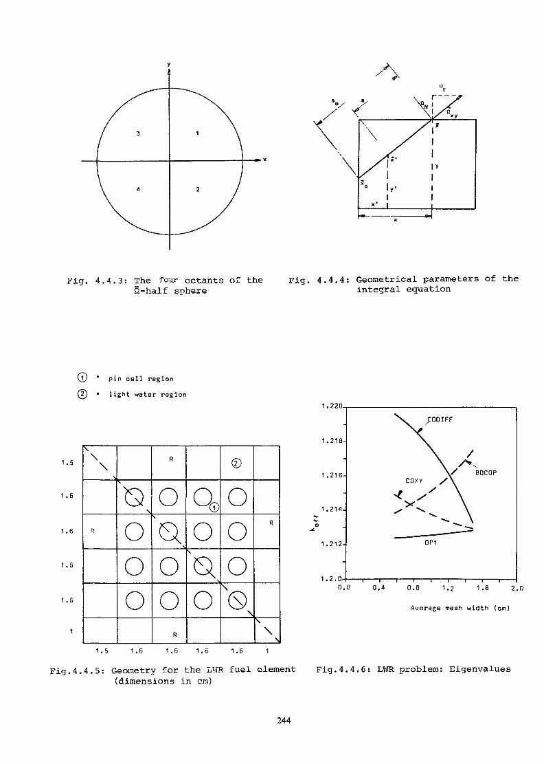
Fig. 4.4.3: The four octants of the Fig. 4.4.4: Geometrical parameters of theH-half sphere integral equation

(1) " pin cell region(2) ' light water region

1.5

1.6

1 .6

1 .6

1 .6

\\\

\

R

S> \

ooo

R

oQoo

R

00

oQo

©

ooo\

\

R

\\

\1.5 1.6 1.6 1.6 1.6 1

1.220.

1.218-

1.216-

1.214-

1.212-

1.2.0-

CODIfF

OP1

0.0 0,4 0.8 1.2 1.6 2.0

Average mesh width (cm)

Fig.4.4.5: Geometry for the LWR fuel element Fig.4.4.6: LWR problem: Eigenvalues(dimensions in cm)

244

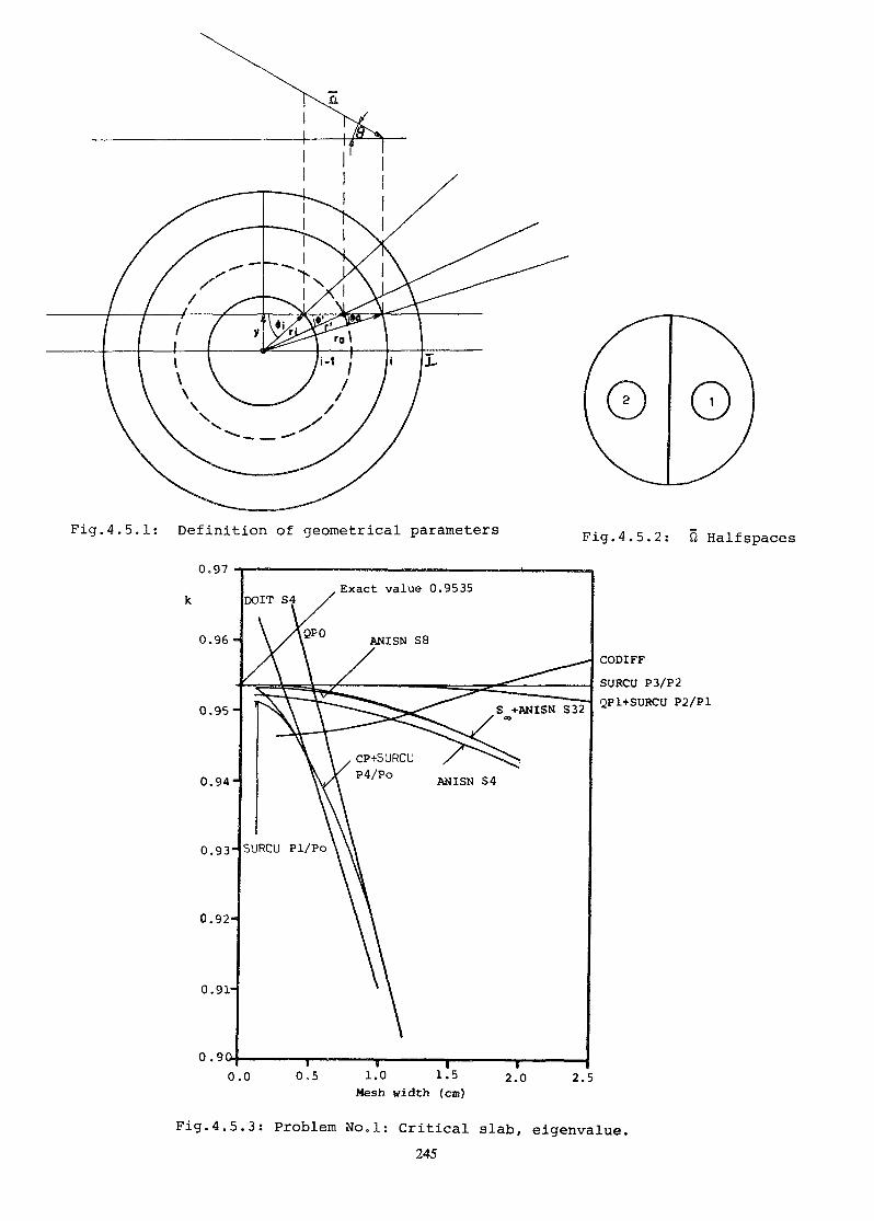
Fig.4.5.1: Definition of geometrical parameters

0.97

0.96-

0.95-

0.94-

0.93-

0.92-

0.91-

Fig.4.5.2: fi Half spaces

0.9Û

CODIFFSURCU P3/P2QPl+SURCU P2/P1

0.0 0.5 1.0 i.b 2.0Mesh width (cm)

2.5

Fig.4.5.3: Problem No.l: Critical slab, eigenvalue.245

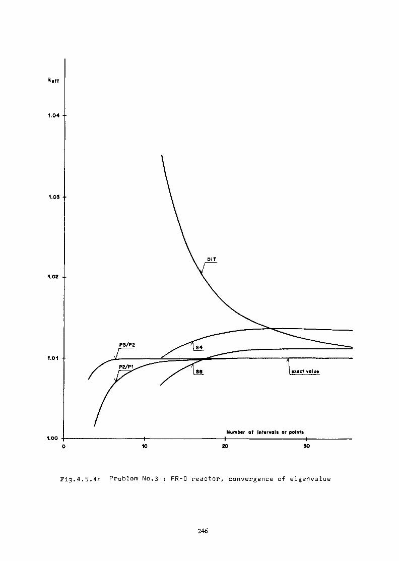
k.ff

1.04 - •

1.03

1.02 - -

1.01 -

1.00Number of intervals or point»

10 30

Fig.4.5.4: Problem No.3 : FR-0 reactor, convergence of eigenvalue

246

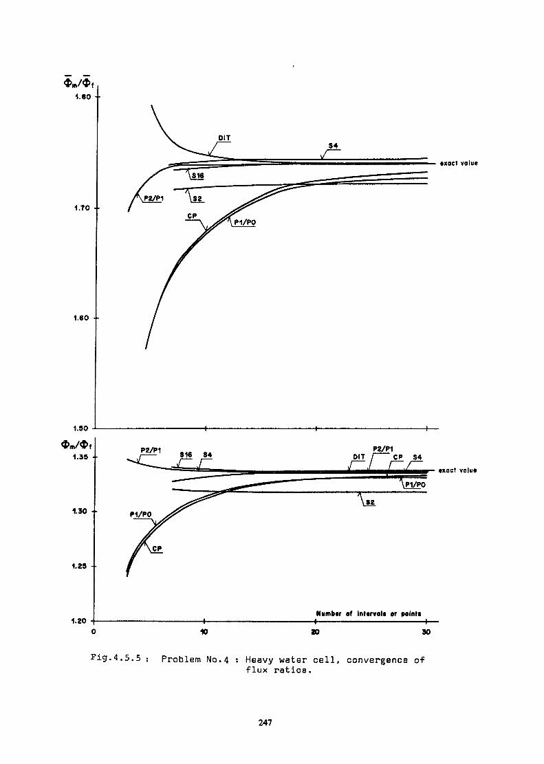
1.80

1.70 • •

1.60 •

1.30

1.35

1.30 •

1.25

1.20

P2/P1 S16 84

'— exact value

P2/P1OIT /—— CP S4

•xact valu«

Number of interval« or points

10 30

Fig.4.5.5 ; Problem No.4 : Heavy water cell, convergence offlux ratios.

247

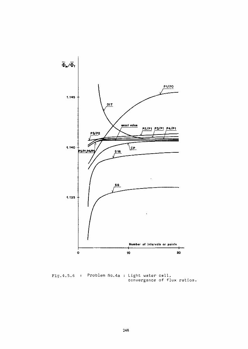
p V PO

Number of Infervels or points

1.133 --

Fig.4.5.6 : Problem No.4a : Light water cell,convergence of flux ratios,

248

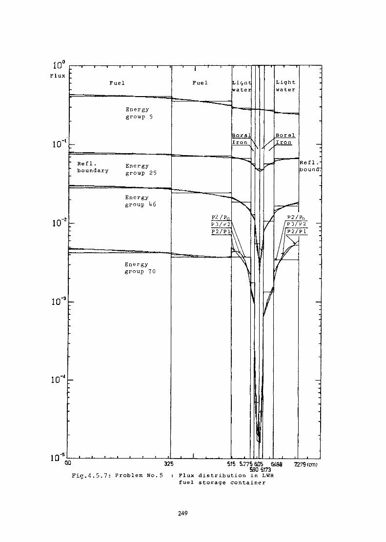
325 5.15 5.775 605 6A98590 &173

Fig.4.5.7: Problem N o . 5 : Flux dis t r ibut ion in LWRfuel storage Container

7279 (cm?

249

s111oü)o

3 —

l l l

1 l

—— EXACT——- ONE SUBZONE—- TWO SUBZONES—

3

r [cm]

Fig. 4. 6. l. : Graphic representation of the right hand side of Eq. 4 . 6 .10

Two-zone fuel-moderator cell, r = 2. 5 cm, r = 7. 5 cm.1 Là

K1 = 1.09, K2= 0.44,Parameter values: C =4 .44 , C = 1,J. Lt

a l= 0.0001, a? =-0.0151, b1 = -18.43, b 2 =-2 .194 .

z

Of.

flC

IS

U

13

12

11

10

9

8

7

6

5

t

3

2

l

0

——— EXACT—— - ONE SUBZONE—- TWO SUBZONES—

Fig.4.6.2

1 2 3 i 5 6

r [cm]

Comparison of exact and approximate analytical solutionsof Eq.k.6.10for the flux moments 0 and 0 . Parameter

values are the same as for Fig. it.6.1.250

123 125 127 129 131 133

> u-ln Eo/EEo=10 MeV

Fig.4.6.3: Lethargy variation of the resonance neutron flux in a

two-zone cell enriched uranium metal - HO.

E [tv]

Fig .4 .6.4: Energy distribution of the neutron flux through the 6. 7 eV

resonance of U-238. Uranium - graphite cell studied by

Lewis and Adler in (5); r = 1.732 cm, r = 7.2 cm.

251

0.1 —

Fig .4 .6 .5 ; Spatial distribution of the neutron flux for the energies

denoted by a-d in Fig. 4.

252

Chapter V

FINITE ELEMENTS AND NODAL METHODS IN DIFFUSION

D.M. DAVIERWALLA, C. MAEDER, F. SCHMIDT

INTRODUCTION

This chapter describes two coarse mesh methods for the solution of themultigroup neutron diffusion equation. The contribution has been keptrelatively short by omitting all references to numerical accelerationtechniques for the iterative solution of linear algebraic equationsarising from discretization.

The two methods described here are the method of Finite Elements and theNodal method. The latter method was contributed by C. Maeder - Eidg.Institut für Reaktorforschung, Würenlingen, Switzerland whereas thesection on Finite Elements was contributed by F.A.R. Schmidt of theInstitut für Kernenergetik und Energiesysteme, Stuttgart University,West Germany and D.M. Davierwalla of the Eidg. Institut für Reaktor-forschung Würenlingen, Switzerland, who served also as the editor.

5.1.1 Finite Elements in Neutron Diffusion.

The Finite Element method was already established in structural engineeringbefore it was first used in the nuclear areas in the early seventies. Asexcellent review articles which compare various coarse mesh methods usedcurrently in neutron diffusion theory we refer the reader to the papers ofM.R. WAGNER (1975) and C.H. ADAMS (1977). In this section the method used byDAVIERWALLA (1977) and SCHMIDT et al. (1975,1978,1979) is described.The ProblemWe consider a domain R with boundary 3R. The equation to be solved is eitherthe external source problem

- V • D(P) V<j.(r) + I%(r) » Q(p) (5.1)or the k problem

- V • D(P) 7*(p) + rVr) - r-i- (vE,(p))*(p) + Q (r) (5.2)eff r s

where Q(r) is an external source, Q (r) is a combined up and down scatteringsource and the other symbols have their usual meaning. The boundary conditionsare of the Dirichlet type

*(r) - f(r) « 0 ; re3RD ; (5-3a)

253

and/or the Cauchy type

q = 0 ;re3Rc . (5.3b)

In addition the solution must satisfy the followinga) $(r) must be continuous in R * R + 3R, the closure of R.b) D • ;' ' must be continuous across material interfaces.3nc) $(r) £ 0 everywhere within the region.

The gethodAn integral formulation of this problem may be derived in several ways. Themost common ones are the functional formulation and the Galerkin procedure.

The former consists in equating to zero the variation, 6j, of the functionalJ, where

(r)) + Z - $ (r)} - Q . (f.(r)Jdr + |ß<fr2(r) + q4>(r)dr (5.U)

3R

Equation (5-1) is the Euler equation of the functional in eq.. (5-1*-).

An approximate solution of the variations! problem

<SJ = 0 (5.5)

can be found by settingNS a.ij/. (5.6)

where the 41. are known trial functions. This is called the Ritz method. Usingthe Ritz approximation, eq. (5.5) may be transformed into a system of equationsfor the unknown coefficients a..

The same system of equations may be obtained by multiplying eq. (5.1) by thetrial function t|i. and integrating over the whole space where the problem isdefined. The integration by parts transforms the second order differentialoperator into a quadratic form in the first order operator as in eq. (5-^)(Galerkin method).

As a result one gets the so called weak form of eq. (5-1) which contains onlyfirst order derivatives . The problem is well defined as long as these derivati-ves are finite, but the continuity of the derivatives is not explicitely required.

254

For more complex problems it becomes difficult to define approximate trialfunctions. Therefore we divide the solution space into nonoverlapping subspaces.We define trial functions for each of these subspaces. For the energy variablewe use constant trial functions. Here the subspaces are called groups. Theunknown coefficients of the trial functions are the group fluxes. The resultingsystem of equations is the well known multigroup formulation of the diffusionequation. The multigroup formulation to the problem defined by eq.(5-l)-(5.3) has the form given below.

For all groups g = 1, N the following holds in R

« ff , s ff*~Kflr o_ vu ürfl A t 5* —• \*O O] A —v T s i <f

(5.7)Xv* Z "i* *8' * Z

g' g'*gand at the boundary 3R

g+ ag<|>g + qg = 0 ; r* R\o ï l r i ( 5 . 0 )

with

<(>g group fluxD diffusion constant in group gg S ' "*"Ä K2T' B ' 2f cross sections as usual (total, scattering fission)gX fission spectrum

A, smallest eigenvalue with k = 1/X1v yield of neutrons per one fission»Q external source in group gg g

at , 4 boundary constants3* irr I normal derivative at the boundary 3R3n 3R

Now for each of these group equations there exists again a functional similar tothe one in eq. (5« ). The solution function <j>S depends only on the spatialcoordinates. The functionals for the different groups g are coupled throughthe fission and scattering source terms.

(5>9)

6'

255

\ ! (agU«)2 + 2qV) d3R3R

for g, g1 - 1, 2, ... N .u

For each group equation (5-10) an approximate solution of the form of eq.(5-6) may be developed. However, it is far simpler to divide the region Rinto M nonoverlapping subdomains which exhaust the region. For simplicity weuse the same subspaces for all energy groups. These subspaces now are calledfinite elements. The shapes of these elements can be choosen quite arbitrarily.However we shall restrict our practical considerations to quite simple shapeslike triangles or prisms with straight or curved boundaries. Also we shallassume for the theory of this chapter that each element contains only onematerial. Again this assumption is not essential.

The introduction of finite elements with separate trial functions allows afurther splitting of the group dependent functionals

_MJ m g (5-11)

m=1where the summation extends over all the finite elements.

In each element we approximate the solution as follows

mg mg$(x,y,z) « W(x,y,z) = /_, k*S- (x.y.z) (5.12)

The functions Ç (x,y,z) are called basis functions. We use the same functionswhich were introduced as trial functions. The basis functions are now definedonly in a corresponding finite element and disappear outside this element.Different basis functions may be used for different elements. However one hasto assure the continuity of the solution in the element andacross the boundariesof adjacent finite elements. The continuity inside the finite element can be gua-ranteed by the use of continuous basis functions and the continuity across bounda-ries can be achieved by an appropriate selection of the weighting coefficientsmgk . One possibility is to select nodes for each element in such a way that eachnode corresponds to one weighting coefficient.We require

for all nodes i = l, L

256

Thus the weighting coefficients become values of the solution at the nodes

ormg mg

W(x,y,z)mg

(5. 15)

We position as many nodes onto the element surface as are necessary to definethe solution at the surface. We can eliminate the dependence of the un-knowns on the element by setting

for all unknowns which belong to the same node. This also guarantees the con-tinuity of the solution along boundaries.

Having eg.. (5-15) in mind we can consider the unknowns as independent.Therefore,the vanishing of the variation of the functional Js means that thepartial derivatives of the functional with respect to all unknowns have to bezero.

(5.17)

The contribution from every element which shares the node (x ,y , z ) must betaken into account. The contribution of a single element may be written as:

m t u1 'm

g«

- rEg _*- m m U_

m

sg' m g1 + \ vg'+g ,m g1fm H Z_j S *«,

g'fg m

Here the external source is approximated by

m

(5.18)

dV

S ' (5.19)

For external boundary elements the contribution of the form

m257

may have to "be added in case of the Neumann boundary condition and the contribution

m

to account for boundary sources. The sum of the expressions (5.20) and (5-21)corresponds to the contribution of the boundary conditions of the Cauchy type.

Again the source term is developed in a way similar to eq. (5-19):

(x,y,z)

We introduce auxilary matrices [dj, L^J, and LrJ to describe the integrationof the various combinations of basis functions:

d „ = /(VÇ • V Ç . ) dV = < 7Cn,i v *n l *

*n.*

r

We further introduce element matrices [ks] , [sg "^ , and £fs 3 by

[k*] = D« • [d] + (r{ - if«) [t] + a« ' [r]

L8 J - *s L^J (5.2l*)

[f8'] » vrg'. [t]

Now for the element m we can rewrite eq. (5.18). The result is

[fs ]m . {$s >m ( 25)

-t^ - Mm • {Qs>m + Hm • t*«),If we combine the contributions of all elements of one group with the con-dition introduced in eq,. (5.l6) we get as a discretized form of the groupequation

258

26)

t- [T] • {Q8} + [R] • {q8}

The matrices [K8] , [S8 "* J , p"8 ] , [T] and p?] correspond to those definedfor the elements using small letters. They are quite sparse and in general with-out any regular structure. In diffusion theory the matrices are symmetric andpositive definite. We shall return to these properties in the third section.Further details may be found in DAVIERWALLA (1977).

5.1.2 The Finite Elements

The implementation of the finite element method in a computer program requiresseveral decisions. One of the most important is the choice of the finite elements.A finite element is characterized by its shape, by the kind of basis functionsused and by the order of the approximation. As yet only the Lagrangian andHermite types of elements have been used in nuclear reactor applications andusually in connection with X-Y or R-Z geometry, see HANSEN & KANG (1975), SCHMIDT(1975), KAPER LEAF & LIÎTDEMAN (1972). However, polynomials up to order two seemto be sufficient for most purposes.

In applied mathematics elements using splines as basis functions have been con-structed. However, these elements have, as yet, made no inroads into nuclearreactor codes. Polynomials as such have only their simplicity as a recommendation.In theory we try to obtain an everywhere nonnegative solution for the flux. Withpolynomials this is not possible and we must expect the flux to become negativeat a few nodes at least locally. This is not a serious problem. We have alwaysfound that the few negative flux values which occur have always been accompaniedby very small amplitudes and it was possible to remove them by refining the mesh.Splines should be able to remove this flaw. It is reasonable well known that ra-tional functions are superior approximants to monotonie convex or concave functionsthan polynomials; so that the efforts of E. WACHPRESS (197l) deserve more attention.

The shape of the elements seems still to be an unexplored field. Triangles orrectangles are commonly used in two dimensions. This leads to discretisationswhich are very similar to the ones known from finite difference calculations.Also, the integrations necessary to define coefficients in eq. (5.26) may be doneanalytically for these types of elements. However, more complex elements similarto the ones used in structural mechanics may also be employed in reactor physics.

For those elements numerical integration procedures have to be applied forthe evaluation of the element matrices. This allows the introduction of curvedboundaries as well as cross sections which are both anisotropic and spatiallydependent inside a single element.

259

Other areas which are influenced by the types of elements choosen for aspecial program are

a) the net generationb) the display of a net especially in three dimensionsc) the description of the elementsd) the modification of a discretisatione) the solution algorithm for the group equationsf) the display of the results.

5.1.3 Elements with varying cross sections

In order to achieve a maximum advantage of the coarse mesh character of theFinite Element Method it is necessary to have large homogeneous areas. Reactorsdo not always offer this situation so that the storage problem becomes acute andit becomes necessary to extend an element over more than one material. This becomeseven more necessary for depletion diffusion calculations, see DEPPE and HAUSEN(197*0, KAVEKOKY and LAUTAED (1977) and SAPPER (1976).

There are other approaches to the solution of the storage problem avoiding theextension of the elements over more than one material. However, it is connectedmore to the organization of the computation process than the definition of anyspecial element type. This topic is treated in sections 5.1.5 and 5.1.6.

5.1. Solution Techniques

The multigroup diffusion boundary value problem, as opposed to a single group,problem, is not self-adjoint. However,only self adjoint problems can be treated by theminimization of a functional. Hence, a group by group solution procedureusing outer iterations becomes mandatory for finite element codes. Thisprocedure can be implemented in a way similar to the ones known from finitedifference techniques. Basically we use a power iteration technique. It maybe accelerated by source overrelaxation, source extrapolation, Tschebysheffor upscatter scaling. (see Chapter 2).

For the solution of the group equations we have compared Cholesky, SuccessiveOverrelaxation and Conjugate Gradient algorithms. Reasons for the use of theConjugate Gradient Method for large matrices are:

a) If one applies the finite element method to diffusion theory problems onegets well conditioned sparse matrices. In reactor physics we are lookingfor the smallest eigenvalue of the whole system only. Both facts favouriterative procedures at least for very large system matrices.

260

On the other hand the matrices vill not have any regular structure by defini-tion. Also the density of nonzero elements is higher than in matrices resultingfrom finite difference discretisations. Thus most of the fast and efficienttechniques for the inner iteration which were developed for the regularstructure of a finite difference mesh net cannot be applied. These factsfavour the Conjugate Gradient Method.

b) The Conjugate Gradient Method has several attractive features: It leads tovery accurate solutions with rounding errors being less pronounced than withdirect solution routines. The convergence is almost independent of thecomputer word length as long as the required accuracy does not conflict withthe word length of the computer. Also one may utilize almost the full wordlength of a computer by using simple double precision arithmetic for thevector multiplications. By scaling the system matrices with its own diagonalelements one may accelerate convergence considerably. For many problems only3 to 5 inner iterations are necessary per outer iteration.

At this stage it should be remembered that the work reviewed here was performedin independent groups and in different countries. It is but natural that not allparticipants will agree with each other on every point. There are some extremelystrong arguments in favour of using direct methods such as the Choleski de-composition • Firstly, a large computation may be performed as a sequenceof smaller problems, large sections of which (the section graphs) are decoupled.Since the matrix corresponding to a section graph is only a fraction of theorder of the original system matrix rounding errors can be kept to a nonsignificant level. Furthermore, any round-off errors generated in a particularsection graph cannot propagate into another section graph. The bulk of thenumber of equations of the original problem are the equations which representthe section graphs. Any error propagation can occur only in the cut set equations -the number of these is minimal if the graph-theoretic separator chosen is alsominimal.

A further point in favour of using direct solution methods is that numericalacceleration schemes such as developed by Lebedev (see chap. 2) are more effectivewith direct solution techniques.

5.1.5 The method of disections

The method is actually a means for cutting up a large problem into a sequence ofsmaller problems. The advantages that accrue from such a procedure are fourfold:a) Only a part of the problem is in core at, any given time. This implies that

central memory cost is considerably cheaper.

b) In finite element problems the ratio of the nonzero entries, in the lower trian-gular half of the system matrix, to the storage required for them by a

261

Jenning's vector,' is low. This implies a poor packing density of the corememory. Whereas, for large problems a ratio as bad as 0.1 to 0.2 is not un-usual, for smaller problems (pieces) it is quite easy to achieve 0.7-0.8.

c) The number of "long operations" (multiplications and divisions) employed by2 3most solution algorithms is between 0(n ) and 0(n ) where n is the order of

the matrix. The same matrix split into m equal parts would require betweenmO((—0 ) and mO((—) ) "long operations". In practice the savings are not quitem mas dramatic because other supplementary work has to be performed when operatingwith a sequence of problems.

d) The size of the problem that can be handled is limited only by peripheralstorage (disc) and not by the central memory.

It is convenient to describe the method of disections in terms of graph theory.To this end we introduce a few elementary definitions(ROSE (1972)).

We realize that any matrix A = (a..) may be regarded as a graph. The row andcolumn subscripts may be viewed as node or point labels and if the entrya.. 0 then there exists an edge joining points i and j.i J1) A graph G(X, E) consists of a set of nodes X and a set of unordered

pairs of nodes, {x,y} called edges. The edge set is denoted by E.

2) A subgraph G'(X!, E') of G is a graph with X'grX and E'c=E.

3) For YÇTX the subgraph G(Y,E(Y)), of G(X, E) withE(Y) = ! {x,y} eE 1 x,y e Y ( is called a section graph.

k) A separator of a connected graph G(X, E) is a nodal subset SCZX such thatthe section graph G(X\S, E(X\S)) consists of two or more connected components.

5) A separator is minimal if no proper subset of S is also a separator of G.

6) Two vertices of a graph are adjacent if they are connected by an edge. Thusadj(x) = yeX | {x,y} eE

7) Similarly, for a proper subset of nodes Yc= X, the adjacency is defined as

adj(Y) » lxeX\Y | 3 yeY ; {x,y} e E j -

8) An ordered graph on n nodes, denoted by G = G(X,E,o) is a graph whose nodeshave been labelled by a bijection a : {1,2, . ...n}-*-»- X

9) The set of vertices monotonely adjacent to a particular vertex x, is denotedby Madj(x) = adj(x)f|{yeX i a"1(y) < a~1(x)}

262

In other words the set of vertices monotonely adjacent to a particular nod.?are those nodes which are connected to x by an edge and additionally have ulabel smaller than that of x.

10) If nodal subsets are labelled in an appropriate hierarchical order monotoneadjacency of these nodal subsets may be defined in an analogous manner.

5.1.6 The computer implementation (DAVIERWALLA)*

The domain over which the solution is sought is covered by a circumscribingrectangle, which is cut up into smaller rectangles by X and Y cuts i.e.straight lines parallel to the Y and the X axes respectively. These smallerrectangles are triangulated and those which fall within the domain are theelements. The elements are labelled and the result is called an element map(LMTMAPilt is clear that the boundaries, of the element map interior to thedomain are the cuts. It should be noted that the element maps are disjointgeometric arrays of element labels which exhaust the set of all elements.Furthertthe cuts partition the nodes into disjoint subsets. Those nodeswhich correspond to a section graph are numbered first. The process continuesuntil all section graph nodes have been labelled. Next all nodes on the Xcuts are numbered followed by those on Y cuts. Finally the nodes on the inter-sections of X and Y cuts are labelled. Thus the totality of nodes are parti-tioned into disjoint subsets. To each of these nodal subsets we assign a setof elements denoted by LMTSET. An element qualifies for inclusion in particularLMTSET if and only if it has at least one node on the corresponding nodalsubset. This is accomplished by subroutine FORMSET. For each LMTSET subroutineSETADJ determines the monotone adjacencies for the particular LMTSET. Theresults are stored in a binary vector IVEC whose j-th cell is unity if thej-th LMTSET is a neighbour and possess a lower label than the LMTSET underconsideration.

The ensuing computations follow normally until we reach the Choleski decompo-Ts it ion. The classical Choleski decomposition is given by LL = A where

j-li. [ a. . - ) I.. A.. ) /A.. j=l,2...n

V*J L •* lk/ W i.<j+l),.

* To be published.263

The only modification required to convert the above to the variable band widthCholeaki method is to replace the lower summation index by the maximum of thecolumn indices of the first nonzero entry in rows i and j.

If the problem is split up by cuts, then as long as the index of the subproblemis less than or equal to the number of section graphs the decomposition proceedsas indicated above.

Once the index of the subproblem exceeds the number of section graphs theresulting Choleski block is either rectangular or lower triangular. The re-ctangular matrix blocks are a result of connectivity between nodes belongingto distinct subsets, whereas triangular matrices are a result of edges joiningtwo nodes in the same nodal subset.

R>r I greater than but J less than the number of section graphs the rectangularCholeski factor is

T -ITBIJ ' LJJ AIJ

v/hen both the indices are greater than the number of section graphs the resultingfactor is

m _T tJ -L mm

BIJ * LJJ (AIJ - BIK V

where in the so called fill-in case A_j can be nonexistant. Finally for I=Jwe get

J-l«Jv J J J(J uK JKK=l

We have had this system in operation for a little over a year and testedit thoroughly.As a validation for the disection scheme we have taken smallproblems and run these with and without disections. The results have talliedto the twelfth decimal digit. By disecting a problem suitably we have beenable to run any problem in TO - 100 K. memory including the program. Asmentioned earlier the equations corresponding to the section graphs constitutethe bulk of the total number of equations. Hence a little reflection willindicate that the maximum core requirements will occur during the computationof

T -lB a L Alu Id U

for some I greater than the number of section graphs but with a J smallerthen the number of section graphs.

It should be brought to the users attention that when a problem is run with-out any cuts, if at all possible, the time per iteration is smallest butthe cost per iteration is high. Cuts have always resulted in cheaper runseven if a little slower.

To date only a two dimensional scheme has been implemented. It should benoted that the nodes of a section graph are distributed over subregionsof the same dimensionality as the original problem. The cut set nodes aredistributed over regions of sucessively lower dimensionality ie.line segmentsand points. The extension to three dimensions is reasonably straight forward.The nodes of the section graphs are distributed over three dimensional regions,whereas cut set nodes are distributed over cut-planes, over line segmentsformed by the intersection of cut-planes,and cut-points.

5.2. NODAL METHOD

5.2.1 Definition of the nodal method

Consider a system which is divided into homogeneous volume elements called nodesor meshes. The nodal method deals with average quantities such as the averageflux of a node, higher order spatial flux moments in the node and average meshsurface currents. To determine these quantities it is chosen to solve the one-dimensional diffusion equation with transverse leakage.

5.2.2 The analytic nodal method

The diffusion equation and Kick's law are integrated in a node over all but onespace variables. The resulting equations are solved analytically assuming aparticular form for the leakage in the transverse directions. The flat leakageapproximation (SHOBER (1977)), a two-step function (SHOBER (1978)), and aquadratic approximation (SMITH (1979)) have been used. A system of equationsi's obtained containing the average flux and the transverse leakages of theconsidered node and its neighbours as unknowns.

5.2.3 Nodal expansion methods

The neutron flux in a node is expanded into a set of functions. Its expansioncoefficients are determined from the given incident partial currents and bymeans of a weighted residual procedure. Orthogonal polynomials with built-inboundary conditions (FlNNEMAKN (1977)) and (SHOBER (1977)) and Legendre poly-nomials (MAEDER (1978)) have been used as expansion and weighting functions.

265

With no further assumptions the response matrix method (WEISS (1977)) isobtained. In the nodal method the calculation of higher order surface currentmoments and of flux moments belonging to expansion functions with more thar;one space variable is avoided. This is achieved by considering only one-dimensional weighting functions and by assuming a certain spatial shape forthe currents in the transverse directions. For the transverse currents aquadratic approximation (BENNEWITZ (1975)) and a linearized form correspondingto the finite difference diffusion theory (FINNEMANN (1977)) have been proposed.These transverse leakage approximations are equivalent to considering crossterms in the flux expansion functions.

Different procedures are possible to solve the resulting equations for thesurface currents and the flux moments in a given mesh. The quantities belongingto each space direction can be determined in an iterative manner by using thelatest values that are available for the transverse directions (FINNEMANN (1977)).In this case a direct solution over all energy groups can be found, and thehigher order flux moments and the coefficients of the flux and current equationsdo not have to be stored. Alternatively the energy groups are treated indivi-dually by means of the fission source iteration technique and a direct solutionin an energy group is performed (MAEDER (1978)). The needed escape and trans-mission probabilities are determined in advance of the flux iterations. In thenodal Green's Function method (LAWRENCE (1978)) the one-dimensional diffusionequation with transverse leakage is converted to an intergal equation by usingthe Green's function. This equation is solved by polynomial flux expansion.

5.2.k 2-D and 3-D IAEA LWR benchmark problems

During the last years many solutions of the IAEA light water reactor benchmarkproblems have been reported. Some results are collected in the TABLES I and II.The most exact solutions which served as reference are described in the Argonnebenchmark problem book (1977).

A very accurate solution with one mesh per subassembly is obtained with theresponse matrix code CIKADA. Because of the large number of flux and surfacecurrent moments that have to be calculated the method is time-consuming andmost useful to produce almost exact solutions for benchmark problems (WEISS(1978)). The nodal Green's function method NGFM shows a very small maximumpower error. Maximum power errors below 2% are produced by the analyticnodal method with the quadratic approximation for the transverse leakage(QUANDRY), by the nodal expansion programs (IQSBOX, MEDIUM-2 and NODLEG)and by the finite element method with 3rd and Uth order flux expansion(TRIDENT and FINELM). The 2nd order finite element method (DIFGEN andFEM3D), the coarse-mesh expansion method (CUBBOX) and the one-group methodswith asymptotic-transient flux representation (MUSIC and SIMULATE) leadto larger errors.

The computing time of a program depends not only on the flux calculationprocedure, but also on the adopted acceleration methods and programmingtechniques. The fastest codes are the analytic nodal program QUANDRY, thenodal expansion programs and the program based on the nodal Green's functionmethod. It is astonishing that the one-group methods do not lead to smallercomputing times than the more accurate nodal two-group programs. Exceptfor TRIDENT the finite element programs are by an order of magnitude slowerthan the nodal programs for these LWR-problems. However, the finite elementmethod has shown so far a greater geometrical flexibility, since it hasbeen extended to r-z- and hexagonal configurations.

a Explanation of symbols in TABLES I and II

- H = Order of flux approximation; in brackets order of approximation fortransverse leakage.

- Ap = Maximum error in subassembly power distribution.

- AP = Average error in subassembly power distribution (standard deviation),

- Equivalent CDC 6600 times are obtained by assuming*Is CDC 6600 = 0.5 s CYBER 175 = 2s CYBER Ilk = 0.5 s IBM 360/195= 2/3 s IBM 370/168 = k s CDC 61+00 = 20 s B-6700 = l s IBM 360/91

- NIT = Number of outer iterations.

- e * Pointwise flux convergence parameter between outer iterations.

- The reference refers to the paper where results are reported.

* The computing time comparisons were deduced from the papersAEEW-R 988 (1976) and K.D. Lathrop, "Computational proceduresfor multidimensional core analysis", CONF-7801+01 (1978).

267

TABLE I. RESULTS FOR 2-D IAEA PROBLEM

Code

MEDIUM-2MEDIUM-2CIKADANGPMNODLEGQUANDRYFINELMb

FINELMb

DIFGENCUBBOXMUSICSIMULATE

TRIDENTTRIDENT

N

5(2)5(2)33(2)5(2)«(2)3U26oo

oo

33

Mesh

51x519x99x99x99x99x99x99x92319 nodes9x99x99x9

9x93Ux3U

keff

1.029591.029661.029581.02961*1.029591.029621 . 029771.029621.029581.029531.02986

1.029691.02958

AP (JOMax

-l.U0.0O.U1.00.9U.O1.0O.U3.02.65-3

l.U0.0

AP (JOAv

_

0.0

0.30.31.8O.U0.20.81.01.6

-0

Computer

CYBER 175CYBER 175

CYBER 175CDC 6UOOIBM 370/168CDC 6UOOCDC 6UOOCYBER 17U

CYBER 175

IBM 360/91IBM 360/91

Comp.time (s)Actual

15.10.9

2.1271.268160UOO

U.7

6.33U

CDC-6600

302

U7217UO200

9

63U

NIT

U2

3828

262638

1818

c

1.0-51.0-5

1.0-51.0-51.0-51.0-51.0-51.0-5

1.0-31.Û-U

Ref.

WAGNER (1977)WAGNER (1977)WEISS (1977)LAWRENCE (1978)MAEDER (1978)SMITH (1979)DAVIERWALLA (1979)DAVIEHWALLA (1979)SCHMIDT (1978)LANGENBUCH (1977)BONALUMI (1978)ANCONA (1978)+ BOKHAREE (1978)KAVESOKY (1979)KAVENOKY (1979)

K)O\OO

a Explanation of symbols (cf. page 23)t 2 triangles per rectangular mesh were used as elements

TABLE II. RESULTS FOR 3-D IAEA PROBLEM**

Code

VENTUREVENTUREQUANDRYIQSBOXNODLEGFEM3DDIFGENb

DIFGEN0

N

11-(2)5(2)5(2)122

Mesh

Extra-polated102x102x11»9x9x199x9x199x9x1916x16x13252x11252x13

keff

1.029031.028961.02901»1.029111.029081.02921.029121.02928

AP (%)Max

2.10.70.91.0U.I

AP (%}Av

1.00.20.30.1»2.1

Computer

IBM 360/195IBM 370/168CDC 6600CDC 61»00B-6700CDC 6600CYBER 17l»

Comp.time (min)Actual

3600.518.6

138018.631-5

CDC 6600

7200.7127018.616

NIT

1»1»367113858

e

1.0-51.0-1»1.0-51.0-51.0-35.0-1»1.0-1»

Ref.

ARGONNE (1977)ARGONNE (1977)SMITH (1979)WAGNER (1977)MAEDER (1978)ARGONNE (19Ï7)FRANKE (1977)SCHMIDT (1979)

too\

a Explanation of symbols (cf. page 23)b Tetraedric elementsc Prismatic elements

REFERENCES

C.H. Adams, (1977), Current trends in methods for Neutrondiffusion calculations, Nucl. Sc. and Engineering 64552-562

ANCONA, A. et al. (1978), "Coarse Mesh Techniques for Multi-dimensional Core Analysis", CONF-780401 145.

ARGONNE, Code Center (1977): Benchmark Problem Book, ANL-7416,Suppl.2, pgs. 277 and 437.

BEMNEWITZ, F. et al. (1975). "Higher Order Corrections in No-dal Reactor Calculations", Trans. Am. Nucl. Soc. 2_2 250.

BOKHAREE, S. und BECKER, M. (1978), "Albedo Conditions forPower Reactors", Trans. Am. Nucl.Soc. 28 768.

BONALUMI, R.A. et al. (1978), "MUSIC-A Mesh-Unrestricted Simu-lation Code", CONF-780401 169.

DAVIERWALLA, D.M. (1977), "A Finite Element Solution to theNeutron Diffusion Equation in two dimensions", Int. Series ofNum. Math. (INSM) 317 95.

DAVIERWALLA, D.M. and HIGGS, C. (1979), Personal Communicationto C. Maeder.

Deppe and Hansen, (1974), Application of the finite elementmethod to two-dimensional diffusion problems, Nucl. Scienceand Engineering 54, 456

FINNEMANN, H. et al. (1977), "Interface Current Techniquesfor Multidimensional Reactor Calculations", Atomkernenergie 30323.

FRANKE, H.P. (1977), "Anwendung der Methode der finiten Ele-mente bei der Berechnung dreidimensionaler reaktorphysikali-scher Probleme", Atomkernenergie 3_p_ 88.

Hansen & Kang, (1975), Advances in Nuclear Science and techno-logy, Vol. 8.

270

Kaper, Leaf and Lindeinan, (1972) , A timing study for somehigher order Finite element approximation Procedures and alow order finite difference approximation procedure for thenumerical solution of the multigroup neutron diffusion Equa-tion, Nucl. Science and Engineering 49 (27-48).

Kavenoky and Lautard, (1977), A finite element depletion diffu-sion calculation method with space dependant cross-sections,Nucl. science and Engineering 64, (563-575)

KAVENOKY, A. (1979), Personal communication.

LANGENBUCH, S. et al. (1977), "High-Order Schemes for NeutronKinetics Calculations Based on Local Polynomial Approximation",Nucl. Sei. Eng. £4_ 508.

LAWRENCE, R.D. and DORNING, J.J. (1978), "A Nodal Green's Func-tion Method for Multidimensional Neutron Diffusion Calculations",Trans. Am. Nucl. Soc. 2_8 248.

MAEDER, C. (1978), "A Nodal Diffusion Method with LegendrePolynomials" CONF-780401, 121.

ROSE, D.R. (1972), A graph theoretic study of the numericalsolution of sparse positive definite systems of linear equa-tions in Graph Theory and Computing ed. R.C. READ.

Sapper E. (1976) Verfahren um optimale Anwendung der FiniteElemente Methode in der Berechnung reaktorphysikalischer Pro-bleme IKE4-55

Schmidt, F.A.R. Ambrosius, Franke, Sapper, Wagner, (1975),Proc. Conf. computational methods in nuclear EngineeringCONF-750413 PI-1 Charleston, South Carolina, Savannah RiverLaboratory

SCHMIDT, F.A.R. et al. (1978), "Two and Three-DimensionalReactor Physics Calculations for HTR Reactors with the FiniteElement Method", CONF-780401, 399.

SCHMIDT, F.A.R. (1979), "Finite Element Methods for the Solu-tion of .Multidimensional Reactor Physics Problems", IKE-report(to be published).

271

SHOBER, R.A. et al. (1977), "Two Nodal Methods for SolvingTime-Dependent Group Diffusion Equations", Nucl. Sei. Eng. 6_4582.

SHOBER, R.A. <1978), "Improvements to a Nodal Method for LWRTransient Analysis", Trans. Am. Nucl. Soc. 28 251.

SMITH, K. GPEENM.&NNG. and HENRY, A.F. (1979), Recent Advancesin an Analytic Nodal Method for Static and Transient ReactorAnalysis", Extended version of a paper presented *t the ANSTopical Meeting on "Computational Methods in Nuclear Enginee-ring", Williamsburg, Virginia, USA.

E.L. Wachpress, (1971), A rational basis for function appro-x_.Tiation J. Inst. Maths. Applies 8, (57-68)

M,R. Wagner, (1975), Current trends in multidimensional staticreactor calculations, Proc. Conf. Computational Methods inNuclear Engineering, CONF-750413 p 1-1 Charleston, South Caro-lina, Savannah River Laboratory

WAGNER, M.R. (1977), et al. "Validation of the Nodal ExpansionMethod and the Depletion Program MEDIUM-2 by Benchmark Calcu-lation and Direct Comparison with Experiment", Atomkernener-gie 3£ 129.

WEISS, Z. (1977), "Some Basic Properties of the Response Ma-trix Equations", Nucl. Sei. Eng. 6_3 457.

WEISS, Z. (1978), Personal communication to C. Maeder.

272

Chapter VI

REACTOR DYNAMICS CALCULATIONS

J. DEVOOGHT, T. LEFVERT, J. STANKIEWIEZ

1. INTRODUCTION

This chapter deals with the work done in reactor dynamics within the CoordinatedResearch Program on Transport Theory and Advanced Reactor Calculations by three groupsin Belgium, Poland, Sweden and Italy. The work at Université Libre de Bruxelles wasmostly done by J. DEVOOGHT and E. MUND with the help of M. BARDIAUX and I. SARAGOSSI.A large part of the work concerned with the space dependent kinetics code Cassandrewas done in collaboration with CEN/SCK, Mol, MM. A. SIEBERTZ, P. DUGNOILLE, M.GOLDWASSER, J. JOLY. The research program at Swierk was carried by J. MIKA and R.STANKIEWICZ with the help of T. BLENSKI and A. GADOMSKI. The research at the NationalDefence Research Institute, Stockholm, was carried by T. LEFVERT1- -1 with R. SKOGLUNDand S. SODERBERG. The research program in Italy was carried by W. BARAN and T.TROMBETTI under the direction of V. BOFFI.

As the reader may surmise, it is very difficult to report research progress in suchwide ranging field and by lack of space many topics have been left out of the picture[see however references 74 to 80 ]. As for other chapters, this is not a report ofthe state of the art, although some effort has been given to integrate the work donein the current trend.

2. DISCRETIZATION METHODS IN DIFFUSION THEORY

2.1 . General properties of evolution equations and their approximation

Space dependent kinetics problems are not any more exceptional : the research efforthas followed both the development of computer's hardware and the increasing needs ofreactor safety analysis. The main bottleneck is still the large computing time and adoubtful accuracy. The numerical and analytic tools available are numerous amongwhich three will be used below : time discretization, successive generations andLaplace transforms. The choice of the method leans heavily on the nature of the pro-blem to be solved. For instance, for small heterogeneous subcritical assemblies,transport effects may be important, like time delays or wave fronts. On the otherhand for large power reactors, the volume of computation is the main limiting factor.

In the first part (diffusion theory) we shall deal with an evolution equation

A(t) 0(t) + QCt) CD

In the second part (transport theory) we deal with an integral version.

Memory storage usually exclude time discretization methods that involve more thanone time step. Converting (1) to an integral equation l-xxx-1 [1 ] :

000 =U(h)0(o) +/ [a^ft-t) + UCh-t)M(t)] 0(t)dto

0(t)dt (2)

(x) Report written by J. DEVOOGHT(X*) Present address : Swedish State Power Board, Dep. ERF S-16287, Vällingby, SwedenWe assume here Q(t) =0

273

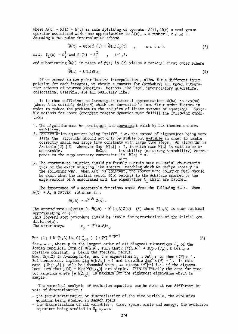
where A(t) = M (t) + N (t) is some splitting of operator A(t), U(t) a semi groupoperator associated with, some approximation to A(t), a a number , o s as 1.Assuming a two point interpolation scheme

= 0Co)£,(t) + 0(h)f2(t) , o< tt h (3)

with f-(o) =6^ and f. (h) =6- , i=1,2.

and substituting 0(p) in place of 0(s) in (2) yields a rational first order scheme

te = C(h)0(o) (4)

If we extend to two-point Hermite interpolations, allow for a different inter-polation for each integral, we obtain a canvass for (probably) all known integra-tion schemes of neutron kinetics. Methods like Fade, interpolatory quadrature,collocation, Galerkin, are all basically like.

It is then sufficient to investigate rational approximations W(hA) to exp(hA)(where A is suitably defined) which are factorizable into first order factors inorder to reduce the problem to the solution of linear systems of equations. Suita-ble methods for space dependent reactor dynamics must fulfill the following condi-tions :

1 . The algorithm must be consistent and convergent which by Lax theorem ensuresstability.

2. The evolution equations being "stiff", i.e. the spread of eigenvalues being verylarge the algorithm should not only be stable but A-stable in order to handlecorrectly small and large time constants with large time steps. An algorithm isA-stable [ 2] [ 3] whenever Sup )W(z) | $ 1, in which case W(z) is said to be A-acceptable. ReZso L-stability (or strong A-stability) corres-ponds to the supplementary constraint lim W(z) = o.

3. The approximate solution should preferably contain some essential characteris-tics of the exact solution like spectral matching which we define loosely inthe following way. When A(t) is constant, the approximate solution 0(t) shouldbe exact when the initial vector jO(o) belongs to the subspace spanned by theeigenvectors of A associated with the eigenvalues X- which are matched.

The importance of A-acceptable functions stems from the following fact. WhenA(t) = A, a matrix solution is :

0(vh) = ev 0(o) ,

The approximate solution is $(uh) = Wv(h,A)0(o) (5) where W(h,A) is some rationalapproximation of eThis forward step procedure should be stable for perturbations of the initial con-dition 0(o).The error obeys £ = Wv(h,A)e0

But [4] II W^h,A) |[ C(V, ) [p (W] V " P + 1 (6)for v •> » , where p is the largest order of all diagonal submatrices J of theJordan canonical form of W(h,A) , such that p (W(h,A)) = sup p (Jr), C being apositive constant, p being the spectral radius. rWhen W(h,Z) is A-acceptable, and the eigenvalues X, : ReX, s o, then p (W) $ 1 .But consistency implies lim W(h,A, ) = 1 and therefore lim p (W) = 1 . In thiscase || ^(hjA) [[ will faeîSboundea when v -*=° except if^=1 i.e. if the eigenva-lues such that p (W) = Maxj W(h,xO[ are simple" This is usually the case for reac-tor kinetics where |W(h^\.,)| is maximum for the rightmost eigenvalue which issimple.

The numerical analysis of evolution equations can be done at two different le-vels of discretization :- the semidiscretization or discretization of the time variable, the evolution

equation being studied in Banach space- the discretization of all variables : time, space, angle and energy, the evolution

equations being studied in R„ space.274

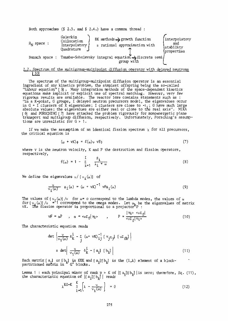
Both approaches (§ 2.3. and § 2.4.) have a common thread :

RN space :CoUocSion ) BK»thods 4 growth functionInterpolator/ f = rational approximation withQuadrature J f»

Banach space : Tanabe-Sobolevsky integral equation discrete semigroup with

interpolator/and

stabilityproperties

2.2. Spectrum of the multigroup-multipoint diffusion operator with delayed neutrons

The spectrum o£ the multigroup-multipoint diffusion operator is an essentialingredient of any kinetics problem, the simplest offspring being the so-called"inhour equation" [ 5] . Many integration methods of the space-dependent kineticsequations make implicit or explicit use of spectral matching. However, very fewrigorous results are available. The reactor lore contains statements such as :"in a K-point, G groups, I delayed neutron precursors model, the eigenvalues occurin G + I clusters of K eigenvalues ; I clusters are close to -X - ; G have much largeabsolute values; the eigenvalues are either real or close to tne real axis". MIKA[ 6] and PORSCHING [ 7] have attacked the problem rigorously for monoenergetic planetransport and multigroup diffusion, respectively. Unfortunately, Porsching's assump-tions are unrealistic for G > 1 .

If we make the assumption of an identical fission spectrum x for all precursors ,the critical equation is

Go = f(o))v vF(j>where v is the neutron velocity, K and F the destruction and fission operators ,respectively,

f U) - 1 - A

(7)

(8)

We define the eigenvalues \>/ [ v -Go)] of

(u + vK) -1(9)

The values of [ v-(u)I /v for u= o correspond to the lambda modes, the values of ufor [ v- (u)] /v =1 correspond to the omega modes. Let w, be the eigenvalues of matrixvK. Tne fission operator is proportional to a projector P :

vF = aP , a = <v££JVx>

The characteristic equation reads

det

P =

..

s det

Each matrix [ a.] or [ bj is KXK and [ a.] [ bj is the (i,k) element of a block-partitioned matrix in G blocks.

Lemma 1 : each principal minor of rank p > K of ][ aJlbJ | is zero; therefore, Eq. (11)the characteristic equation of |[a-][bj | reads

KKG-K X - = 0 (12)

275

Lemma 2 : Eq. (9) has K eigenvalues [v- (u) ] /v , which, are algebraic functions of u.If K = 1, the unique eigenvalue [v^(o))f/v is a rational function of tu.

The eigenvalue problem [Eq. (7)] is the perturbation of a slowing-down problem bya degenerate operator vF. We can apply the Weinstein-Aronszajn theory [ 8 1 : let

W(u) = det [I - vvFCuI + vK)"1] (13)

ThenKG œ - 9V

(14)

where to, and 9, are the eigenvalues of vK and vK - vvF, respectively. It can beshown tftat

K ' 1WCu) = ? ! _ _^__ (15)

and= 0 k=1,... KG (16)

If for some k : e= <* , the degree of the rational function is decreased by one.oFor simplicity we state the following result only for the point model (K = 1) .Theorem I : If the eigenvalues are nondegenerate, a necessary and sufficient con-dition for ui -= a is either <v£~ja >„ = 0 (a) or <yxl C>p - ° (b), where :tne scalar product < \>„ means integration over energy groups; Ify,* ana- \\> ay&

the eigenvectors common to vK and vK -v vF for the direct and adjoint problems,respectively.

The physical meaning of theorem 1 is as follows : the solution of the initialvalue problem without delayed neutrons contains terms like exp(9-t) (correspondingto the full problem) except for a term with exp(w,t) (corresponding to the slowing-down problem) either because (a) the k'th mode does not contribute a net number offission neutrons, or (b) the importance of the fission neutrons produced in thek'th mode is zero. If K = 1 and vF, vK are symmetric matrices (unrealistic assump-tion for G > 1), then the zeros and poles of W(to) are real and alternate, and theYi (to) are all real. This is the case examined by PORSCHING [ 3l . We now turn thedelayed neutrons in.The K(G + 1) eigenvalues of Eq. (7) are solutions of

v,- (to)i _ c, ï (17)

Theorem 2 : (a) [v ,( toJ] /v is real, simple, bounded, smaller than | [ v . ( m j l / v | , i>l™" ' ' ' ~" -- J- if

(b) [ v, ( to) ] /v is monotone increasing for to > u > Re UL• L O K ,

(c) if N > 1 eigenvalues [v . f to^/v are real, where p ?_N numbers[ v.foTl/v < 1,i.

of Eq. (16) are positive and N-p are negative, all in the intervalMoreover, there are N roots in each interval (-\-,1} -*• •) and N in

u j, ~+-,3 ~" <

where \- is the decay constant of the i'th delay ea-neutron precursor.

In practice, we can always take u « -\- All statements about the non-realroots of Eq. (17) are dependent on generalization of the Gershgorin theorem andwill not be dealt with here .

We, therefore, have partly recovered Porsching's results without making any unrea-listic assumptions .

276

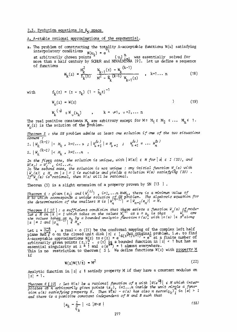
2.3. Evolution equations in R., space

A. A-stable rational approximations of the exponential.

a. The problem of constructing the totality A-acceptable functions W(u) satisfyinginterpolatory conditions ^, -> _ iat arbitrarily chosen points * { u-} ?.. was essentially solved formore than a half century by SŒUR and NEVACNTNNA [9], Let us define a sequenceof functions , rv 11

Mf W. z) -\tK"1JJ\. Jx 1 _____f^_______ __ 1——*t _*

M2 _ w IK-IJ w f7i"i. "^. 1 LZJ

with fk(z) = (z - zk) (1 - zkz)~

W (z) = W(z) > (19)

r ..•!Wk sWv (^Zk : ) ' k= ' v + 2 , . . . n

The real positive constants M. are arbitrary except for M= M^ $ M2 S ... Mn* 1.W (z) is the solution of the problem.

Theorem S : the SN problem admits at least one solution if one of the tao situationsoccurs :

In the fivst aase, the solution is unique, with | W(z)\ $ M for \ z\ é 1 (20), and

In \he second aase, the solution is not unique : any initial function ^z) with| W (z)\ $ M on \z \= 1 is suitable and yields a solution W(z) satisfying (20) .I/V (z) irrational, then W(z) will be rational.

Theorem (3) is a slight extension of a property proven by SN [13 ] .

Theorem 4 : given { z.} and { W(.o)} , i=l, .. .n M=M,, there is a minimum value ofMTto which corresponds a unique solution f£_f^ problem. The algebraic equation forthe determination of the smallest M is \Wn \ = ^n-^z

nn = M-

Theorem 5 [ 10 ] : a sufficient condition that there exists a function WQ(Z) !IMS $ M on \ z \ = 1 which takes on the values W, at z = z^ is that W« ' ar>the values takenjzt z-, by a bounded analytic function a(z), with \a(s) |s UTalong

Let z = -2- , a real < o (21) be the conformai mapping of the coirplex left halfplane Reif* o on the closed unit disk | z| $ 1 ., Our original problem, i.e. to findA-acceptable approximations Wfz ) to a(z) = e l ' J = e at a finite number ofarbitrarily given points {zji1 . a (z) is a bounded function in | z| < 1 but has anessential singularity at z i 1 and a(e ) = 1 aMost everywhere.This is no restriction to theorem [ 3 ]. We define functions W(z) with property Mif

W(z)WC1/2) = M2 (22)

Analytic function in [ z| s 1 satisfy property M if they have a constant modulus onIzl =1.Theorem 6 [ 10] : let W(z) be a rational function of z with \ W(e \ S M which inter-polates at n arbitrarily given points {z.}, i=l...n inside the unit drcte a func-tion v(z) satisfying property N. Then Wlz) - a(z) has also n zeros{c^>2

in \z\ > 1

and there is a positive constant independent of M and TU such that

<L \M-N \

277

Returning to the plane u, we see that if M = N = 1 , to each interpolation point uvin Reu < o is associated another interpolation V, with u. = - V, .

Theorem ? \ 10\ : if the rational function W (z) satisfies the condition of theorem[5 ] 3 "*•* COM be made to interpolate a(z) at an additional point z , providedV W --%If the equality applies and AL = M^ = ... M ^ W (z) is constant and W (z) is theunique function of least maximum modulus innReun£ 0. °

This additional point has no counterpart : we have a total of 2n + 1 interpolationpoints. In practice we have to interpolate e with u = hx at the points u. = hX. ,when h is the time step. When h •> o, the interpolation points move toward! the 1

origin and therefore the minimum value of M given by theorem [4] is a function ofh with lim M '.. (h)=1 . Let now W(z) interpolate a(z) with [W(z) | < M on z| = 1withMÎTi) ^"M, at 2n + 1 points zk = hXk-a/hXk+a.

„ 7 2n+lTheorem 8 [10] : for h sufficiently small, \W(z) - v(s) < c hn | ïï (^~\) Iwith u = yi. When \. = o, W(z(u)) is the diagonal Fade approxi- i=lmant to e .

2 ? ue u.e -W Cu ,u2,M2)= M2. —— ——— 1—— -J ——— - ———— - (24)

b. The general first-order (W^ : first degree of numerator and denominator) isu, u,

u(e + WJ + u.,(e/"., i,. .. \K**'\ — \x^>*n • , <. ,

nw H- w o ' ~i -*• CM*' — w & ' *i

with W.. = M ————— ——————— (25)1 e q 2 - M2

Since eu = ea eu~a, and since - u, is another interpolation point it is easilychecked that W^ (ulu u-jU,) = e W.^(u-aj u^-a, u2~a;1) interpolates e atu19u2,U2 = 2a - UH.However W^ may not be A-acceptable for all values of a.Table I [ 1 ] gives examples of W.., functions. The second order W22 can be writtenreadily by means of (18, 19) but the reduction of well-known approximations(LINIGER-WILLOUGHBY [11] and N0RSETT [12]) to W22 is no easy task [13] .

c. The interpolation points can be used as free parameters to find best A-stable appro-ximations in Chebyshev sense [14] .

The successive application of W(hA) gives, if A(t) = A,

-Wn(hA) |(o)|| = H?"1 W1^) e(n-1"i)hA (eM -i=o

Therefore

- Wn(hA)|(o)|[ _< sup w(h,n ,x) ]ehx - W(hx) | |||(o)|| (26)

with

w(h,n,X) -S Ic^Xh)! eCn"1"i)h (27)i=o

if the spectrum of A is contained in the real interval [ a ,0 ] .If we have an approximant W(hX) which is A-stable and dependent upon m parame-ters yi,,k=1 ...m, the search for the best accuracy at time nh amounts to

Min sup w(h}n,X) | e X h - W ( h X ) | (28)-...J-..

278

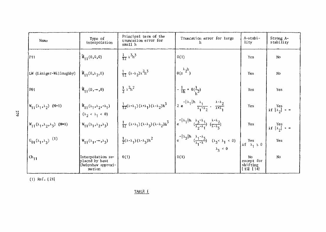
Name

P11

LW (Liniger-WiJloughby)

P01

W (X1 ,x2) (M=1)

W 1 1 (X 1 ,X 2 ,X 3 ) (M=1)

Gni (X1 ,X,) '' 3

Ch11

Type ofinterpolation

^(0,0,0)

^1(o,x2,o)

ftii(0,-°°,0)

ftf r-\ •» -v "i11 V." 1 > ^ 9 t ~~ 1 J

(x2 < x., < 0)

1 1 1 'X2'X3

W1 1 (X,. »-".XT)M l

Interpolation re-placed by bestChebyshev approxi-

mation

Principal term of thetruncation error forsmall h

1 .3,3TTX h

|Y (x-x^xV

i»vJy(x-x1)(x+x1)(x-x2)h3

YJ (x-x1)(x-x3)(x-x2)h

2i - fx-Xn) (x-x,)h1

0(1)

Truncation error for largeh

0(1)

X?h0(e )

- U F * » c ^-|xJh X1 X-X 7

2 e _ -L_ . __ £1 2 1

- |Xi |h X^-X^ X-X7P ' r ^ h r -• iX -X X-X •*2 1 3

-|X3 |h X^XjC v "•»""""" "'\ "•-] L" *Z " 1 ^J

A -t ~~ A J 1

x3 < o0(1)

A-stabi-lity

Yes

Yes

Yes

Yes

Yes

Yesif X1 >, 0

Noexcept forshifting[15] [14]

Strong A-stability

No

No

Yes

Yesi f |X 2 | +~

Yesif |X2 | -»- »

Yes

No

(1) Ref. [21]

TABLE I

The following two cases were investigated : W of first order i .e . , .* withand without spectral matching at one point X , being the leading c eigen-value of A.These new Chebyshev type approximations are A-stable and have the second orderof approximation. Numerical tests have been performed and compared with Faderational approximations and spectral matching algorithm. The results for Che-shev type approximation are the best or closed to the best among these from consi-dered rational approximations except in case of very particular configurations ofthe spectrum of A. For certain configurations of the spectrum the gain of theprecision is significant. The disadvantages of the method are following : theoperator A must be constant, the upper and lower bound of the snectrum is needed,the time step must be kept constant during the whole time internal. The workhas been done in cooperation with Université Libre de Bruxelles and reported in[H].For nonlinear dynamics it is convenient to consider the finite difference appro-ximation which allows for control of the time step during the calculation. GEAR[6] proposed such a technique for multistep method. This method has been usedfor the point dynamics model describing the core and the cooling system withxenon and temperature feedback. The various iterative methods were incorporatedinto the program for solving the nonlinear system appearing at each time step.The method has been tested for some practical problem and the results are presen-ted in [ 1 7] .

B. Runge-Kutta methods with spectral matching.a. General properties : brief review.

Let us review briefly the basic results of Runge-Kutta method C 2 I to be usedbelow.The system to be integrated is

C29)

where î =U0,*r..,<yT ; î= [l,^...^ , = T

The need for A-stability points for implicit Runge-Kutta methods . A R-Kprocedure is a one-step method with m-stages defined by

-HI\ = .; + hv a f CV (30)

where h^ is the time step, a a m x m block matrix, each block element beinga^ I where I is the unit (N+1) x (N+1) matrix. The j component of n^ is

^- -* 'Vector f (n ) is defined by

~

Each î(n ) is a vector with s+1 components :

(31)

t0,~. \,N ] ' i=0°)N (32)

Moreover : n = tv , nj = *.(t^ (33)

bX = \ (34)

280

The R-K system is

*Ctv)m

x=1 (35)

The auxiliary vectors are computed at times t, + c.h , i=1 ...m with

m;.,a«= ciIf the system is linear with constants coefficients : f(ny) = A nuthen

C36)

Ktv)=W(hv,A) Ct^

with the growth functions : W(h ,A) = H + h £T A (IT - h a A") ~1 e (37)

A 0

0 „ A} m ,

m

I 0

0 Im

} m, I being the unit sxs matrix(38)

and e" = [ 1,... 1]Tm

We observe that W(h ,x), a rational function of x , is of order p ifh X

W(h , = e 00$ (39)The maximum order [18] of an implicit m-stage R-K procedure is p=2m. GEAR [19]has shown conversely that to a given growth function can be associated a (nonunique) R-K procedure.

b. R-K methods with spectral matching [13] .

The main defect of solutions of type(2)when A(t)is not constant, is the need todefine some average matrix A. Even so, it is not possible in general to keep theorder p for the local error. On the other hand in many practical cases, A(t), orthe Jacobian of f" is only slowly varying and instantaneous spectral matchinggreatly improves the accuracy. We report below a mean to synthesize both aspectsfor 2 stages R-K procedures defined by

*22

Let p = Tr a, A = det a. Then1 + uCb.+b?-p) + u2(A-

W(h,X) =W(u=hx) « ————— i— i —————up u A

(40)

From (37) a is easily expressed in terms of c,,c2 ,A,p. Identifying W(u) withone of the A-acceptable approximations of e of type (2,2), we have 4 equationsfor 6 unknowns and we are left with a two parameters family of R-K schemes whichallows for interpolation at the origin and two arbitrary points x - i , X2 in Re x <0.

281

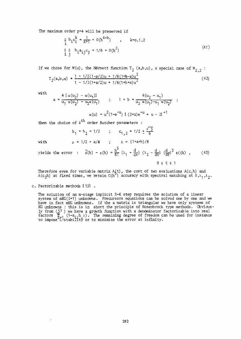
The maximum order p=4 will be preserved ifk _ 1 4-k

It b.a-.c- = 1/6 . 0(h2) (41)i j x 3

If we chose for W(u), the N(6rsett function T? (a,b,u), a special case of W9 :" L y L

T?(a,b,u) = 1 +1/2(1-a/2)u+1/8(1*b-a)u2 (42)

L 1 - 1/2(1+a/2)u + 1/8(1+b+a)uz

4 [a(u7) - a(u,)] 4(u9 - u,)L ___;__ • i + K = . , ' •_. r ,. i * ' *-* _. r_T A TI _ _ / " . " _ ^ ^ *

a(u) = u(1-e"U) [ C2+u)e"u + u - 2]

then the choice of 4 order Butcher parameters :

with p = 1/2 + a/4 ; A = (1+a+b)/85

yields the error : £(h) - <j>(h) = ^- (\1 - ^-) (\2 - ^-) (gjO 41 (çh) , (43)

0 $ ç S 1

Therefore even for variable matrix Aft), the cost of two evaluations A(c.,h) andA(c2h) at fixed times, we retain 0(h ) accuracy with spectral matching at 0 , X - , X 2 >

c. Factorizable methods [ 13} .

The solution of an m-stage implicit R-K step requires the solution of a linearsystem of mKG(I+1) unknowns. Precursors equations can be solved one by one and wehave in fact mKG unknowns. If the a matrix is triangular we have only systems ofKG unknowns : this is in short the principle of Rosenbrock type methods. Obvious-ly from (37 ) we have a growth function with a denominator factorizable into realfactors ff , (1-a..h \). The remaining degree of freedom can be used for instanceto impose1E-stabiiïty or to minimize the error at infinity.

282

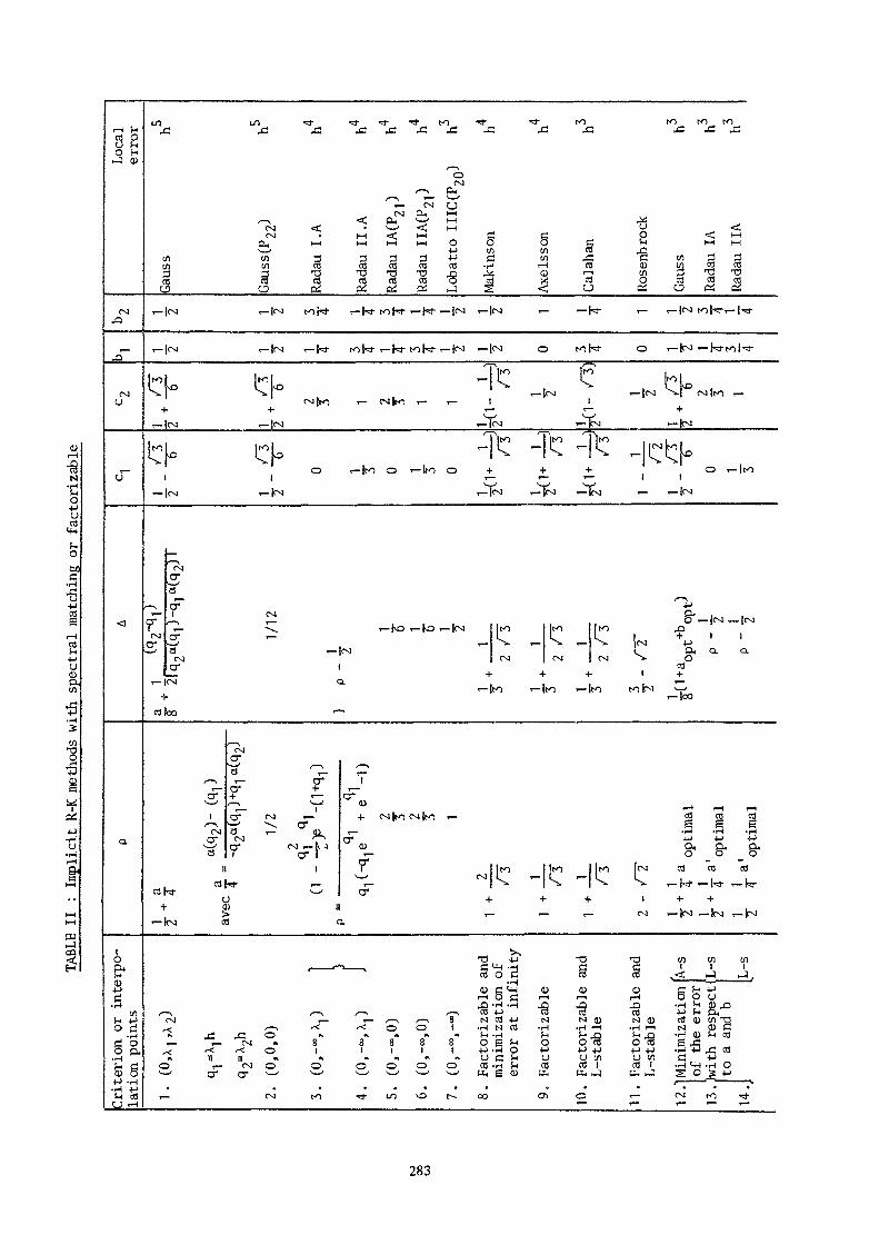
•8N

Octi

•H

•6

S4->U

S,

•H

öS

Î•Hr-l

t

l—lt—<

m

g

rH fH

(VI43

T——

U

o~

<

Q.

Crite

rion

or

inte

rpo-

latio

n p

oint

sU1 LO <3" t3" ^* *3" to ^3" * J" to tO to to

4 2 X 4 2 4 2 4 2 4 3 4 2 4 3 4 2 4 2 4 3 4 2 4 3

O(VI

/•— > O.4

"~r- Cvi CJCV1 CL, hH

^ < O. ^— ' I-H -^ .™ < ' ^ < ^ - _ ^ -vaCVI . |_| < I-H g S O < I-H

p , i — i i — i t — i h - f O O O C M i — i i — i1 — ' -P !/) tf) CO J3<n c/> 3 3 3 3 P ß î / 1 4 3 ß (/> 3 3(/} t/> CO CO CO CO CO *H r*H CO CD (jQ CO CO

CO Co cö cö cö cö o Co X Co O CO CO coo o oi oi oi e: *J 2 < u ci u erf ai

T— |CV1 t— |CVI tOh* t— H- tol'S" t— I C r-|CVI »— |CV1 ,— i— ^ - <-'———'—— 1-

i— cvi v-lcvi ,— | t to he t— hi- to Hs- T- |cvi ,— |cvi o toh* o <— (CM T— N-tol-=r

^Tjto jto" -L to L w I »• , ^ i L to .%. 1 >>. I r- |CVI t— |CVJ .| CVI ItO T—

CV]|to *— CM|lO r- i— 1 1

O i— ItO O r-fco O 4- 4- 4- O i— ItO

— CVI r-|CV] r-ÏCVI r— |cVI T— IcVl i— r- |cvl

CVIcrH'

t— 1 <v]O* r —— > T—I r— "v^ T— K>r— fOt— |CV1 tO tO

£* 2 *~ ^ - k r - k , -

CV1 CVI CV]er i— + 4 - 4

t — |cvi a . i iT— |tO t-|tO <-

cöloo ^

IÔ 43 'r~L 1 4 - 1 1N. cvj +J

T CL, a a.cvi ^v o

cö1 4-

to toN V'r-loO

• — \

f 'T- P/—N r- O* t

t— o* + ^*

£ ï^ ZP û ^ ^ ,_i ç r c v i , — 4-cv i | tocv i | !O i— a j c g c ö^ ^ \ er ^_ . § . § . §er cvi "~ f i ~ +j jj -u

"— ' a* «N» «— k j tu f t Q ^ üa i 3 . l , _ C 3 _ c T _ oH i ^ jlto j|to Ilto [cvi cö cö cö

co HJ- v — ' erO 4- 4- 4- 1 4- 4-

4- CD II i i u> T— r— i— CVI T— JCV1 ^-JCVI T— fVI

T-kvi cö Q.

. ?*•» .^3 4J "^3

cd O C coCD g M-l CD CDi-H S (3 rH rH43 'H -H 43 43/ — \ / — \ / — \ f — \ cö -P cö cö

C V I T — r — , — , , — \ 8 N C O - P M N,< , — v •< •< O O 1 'H M CÖ -H .H

r — , — c v i » 8 S S S S O S ^ O O^ ^ < - < O 1 1 1 1 I P . H O P +->« I I I I « •> » « « « O f i S - i O U

O t — c v i o O O O O O C Ö - H ^ c d CQ

T — c v j t o - * L n o r ~ - c o c n o

1 f f1 TCO v<^ i-J >-J ,

(D C !-• 4->r-l S O O

•S 'O S S/3^3 t^ O cö O V) rÖiH .H r-l N CD ö43 JH 43 -H CD f- CÖcd O cd £ jtf

W) L) CO C P| cd 1 .H 4-1 -H O

r— CVI (O f

283

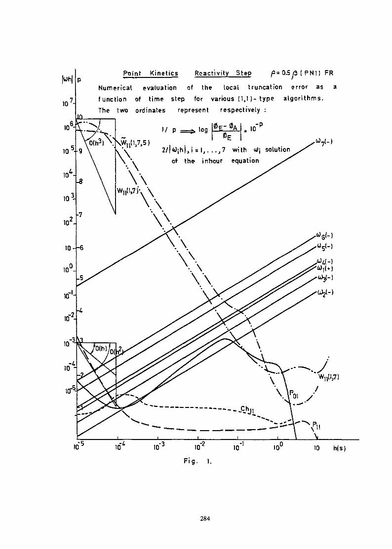
H

10 7-\

Point Kinetics Reactivity Step p= 0.5 ß { PNl) FR

Numerical evaluation of the local truncation error as afunction of time step for various (1,1 ) - t y p e algorithms.The two ordinales represent respectively :

r P

2/|«djh|,isi,. ..,7 with u>j solutionof the inhour equation

10,-5 10* 10.-3 10'2

Fig. I.

10-1 10L 10 h(s)

284

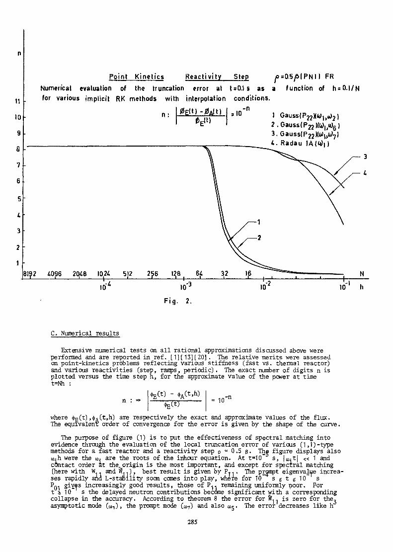
1t

10

9

8

7

6

5

£

3

2

l

Point Kinetics Reac t iv i t y Step f=0.5/S|PNI) FRNumerical evaluation of the truncation error at tsO.is as a function of h = 0.l/Nfor various implicit RK methods with interpolation conditions.

81?2 &096 2048 1024 51?{-

10"

Gauss! P22XWj,2 .3.

. Radau

C. Numerical results

Extensive numerical tests on all rational approximations discussed above wereperformed and are reported in réf. [1] [13] [20]• The relative merits were assessedon point-kinetics problems reflecting various stiffness (fast vs. thermal reactor)and various reactivities (step, ramps, periodic). The exact number of digits n isplotted versus the time step h, for the approximate value of the power at timet=Nh :

- *A(t,h) -n- 10

where <j>E(t) ,4u(t,h) are respectively the exact and approximate values of the flux.The equivalent order of convergence for the error is given by the shape of the curve.

The purpose of figure (1) is to put the effectiveness of spectral matching intoevidence through the evaluation of the local truncation error of various (1,1)-typemethods for a fast reactor and a reactivity step p = O.S 3. The figure displays alsou-h were the u. are the roots of the inhour equation. At t=10~ s, |w^t| « 1 andcontact order at the origin is the most important, and except for spectral matching(here with VL. and "...)» best result is given by P*... The prompt eigenvalue increa-ses rapidly and L-staoility soon comes into play, where for 10~ s $ t $ 10~ sPQI gi-Yf3 increasingly good results, those of P-- remaining uniformly poor. Fort >, 10 s the delayed neutron contributions become significant with a correspondingcollapse in the accuracy. According to theorem 8 the error for ft, , is zero for the,asymptotic mode (o>i), the prompt mode (u7) and also tor. The error decreases like h

285

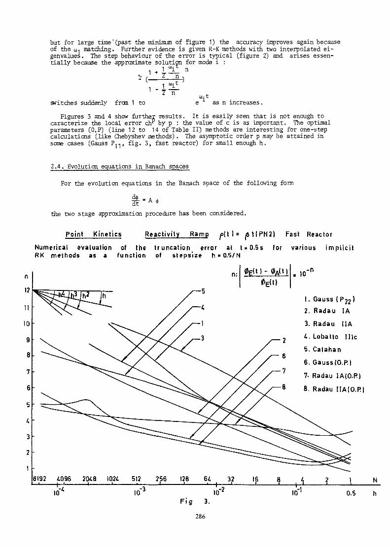
but for large time'(past the minimum of figure 1) the accuracy improves again becauseof the oj-i matching. Further evidence is given R-K methods with two interpolated ei-genvalues. The step behaviour of the error is typical (figure 2) and arises essen-tially because the approximate solution for mode i :

- + 1 Mi n^ r 2" n -,

1 -

switches suddenly from 1 to as n increases.

Figures 3 and 4 show further results. It is easily seen that is not enough tocaracterize the local error ch? by p : the value of c is as important. The optimalparameters (O.P) (line 12 to 14 of Table II) methods are interesting for one-stepcalculations (like Chebyshev methods). The asymptotic order p may be attained insome cases (Gauss P, fig. 3, fast reactor) for small enough h.

2.4. Evolution equations in Banach spaces

For the evolution equations in the Banach space of the following form

A <j

the two stage approximation procedure has been, considered.

Point Kinetics Reactivi t Ramp = |SUPN2) Fast Reactor

Numerical evaluation of the truncation error at t = 0.5 s for various implicitRK methods as a function of stepsize h»0.5 /N

. JO-n

1. Gauss2. Radau !A

3. Radau HA

4. Lobatto lllc

5. Calahan

6. Gauss(O.P)

7- Radau IA(O.R)

8. Radau IIA(O.R)

12

n109

8

7

6

5

4

3

2

I

Point Kinetics React iv i ty Ramp f ( t ) = £ t (PN2) Thermal reactor

Numerical evaluation of the truncation error at t s 0.5 s for various implicitRK methods as a function of stepsize h=0 .5 /N ,

g E l t ) -g A ( t )

8192 4096 2048 1024_j———i_J————i————L_ * 256 JE 64-J-+-

32f

t )= 10-n

). Gauss ( P22 )

2. Radau II A

3. Radau I A

4. Lobatto II Ic

5.Makinson

6. Gauss(P22){O.P)

7. RadauIA(O.P)

N

10* 10

Fig. 4.

ID'1 0.5

It can be illustrated on the diagram

GA(h) —————> CChA)1C(hAn)

where G^Ct) and G. (t) are the semigroups generated by the operators A and A , res-pectively. The passage from A to A corresponds to the approximation of thenoperatorA by the sequence of (A ,X ,P ) where the operator A acts in the suace X and Ptransforms the space X SntB tfie space X . The formuîa describing the local error1(in one time step) has been obtained ana the general stability condition has beenformulated [22] .

However the results for this very general problem have been obtained for ratherstrong assumptions concerning the smoothness of the solution. These assumptions canbe weakened provided that some particular class of evolution equation is considered.

In reactor dynamics model the neutron diffusion equation is of a parabolic type.Thus in further analysis it was assumed that the semigroup generated by A is analyti-cal [ 8] . For the Euler backward formula the following error estimate has been ob-tained [ 23]

ß, 1 ,P (kAt)(44 )

287

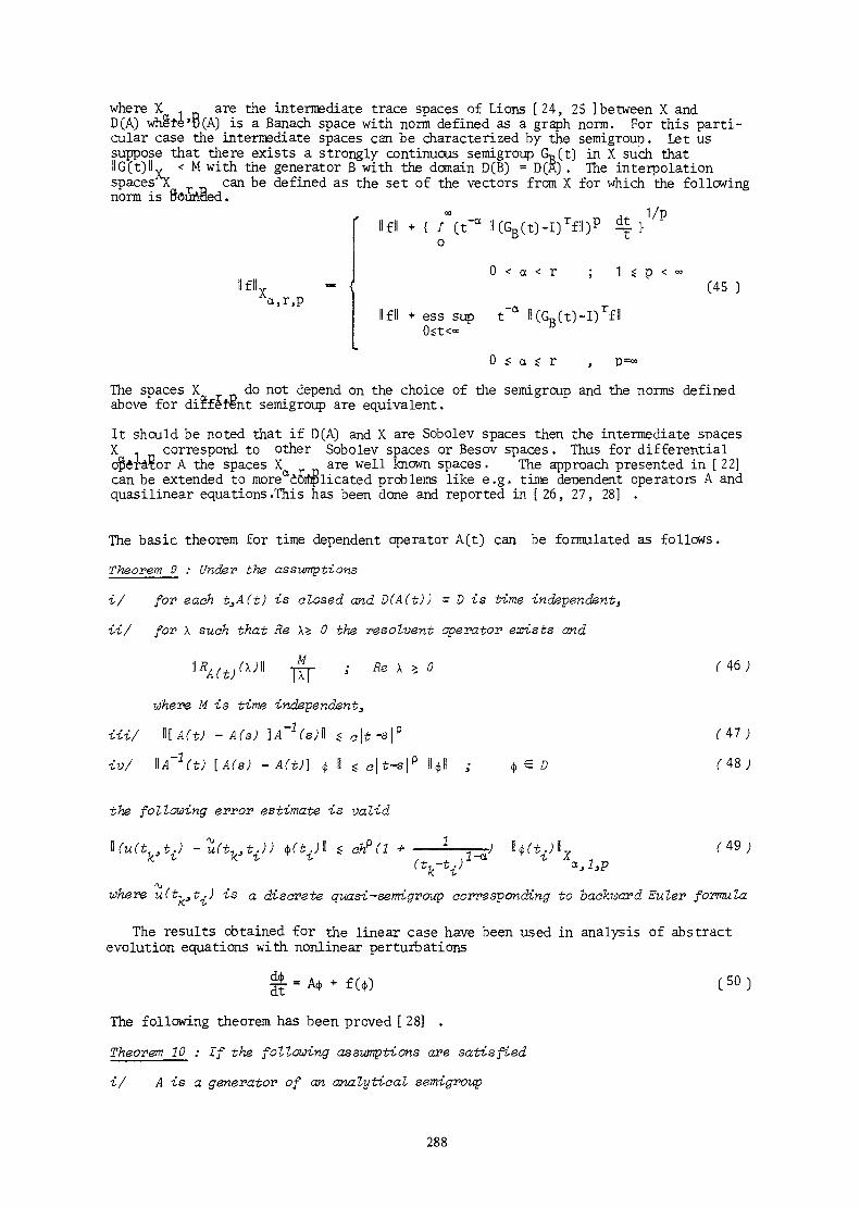
where X . are the intermediate trace spaces of Lions [24 , 25 ] between X andD (A) white'DCA) is a Banach space with norm defined as a graph norm. For this parti-cular case the intermediate spaces can be characterized by the semigroup. Let ussuppose that there exists a strongly continuous semigroup Gg(t) in X such thatliG(t)IL < M with the generator B with the domain D(B) = D(A) . The interpolationspaces^C can be defined as the set of the vectors from X for which the followingnorm is ßdunüed.

00 j 1/PIf« + ( / (t'a «CG B ( tD- i ) r f I ) p %} "

t l f l l0 < a < r ; 1 f p <

a,r,pIf I + ess sup t"a

(45 )

0 $ a s r , p =00

The spaces X do not depend on the choice of the semigroup and the norms definedabove for different semigroup are equivalent.

It should be noted that if D (A) and X are Sobolev spaces then the intermediate spacesX 1 correspond to other Sobolev spaces or Besov spaces . Thus for differentialoperator A the spaces X are well known spaces. The approach presented in [22 ]can be extended to moreacomplicated problems like e.g. time dependent operators A andquasilinear equations .This has been done and reported in [ 26, 27, 28] .

The basic theorem for time dependent operator A[t) can be formulated as follows .

9 : Under the assumptions

i/ for each t,A(t) is closed and D(A(t)) = D is time independent,

ii/ for \ such that Re Xz. 0 the resolvent operator exists and

l]RA(t)(x)]l TTT > Re x * ° ( 46)

where M is time independent,

Hi/ \\[A(t) - A(s) }A~1(sW $c\t-s\P ( 47 ;

iv/ IU~2(t; [ A ( s ) - A(t)} <j> Ii $ c\t-s\(1 Hcf>li ; $ 6 D ( 48 ;

the following error estimate is valid

,t.) -u(t1ttJ) *(t.)\ s ch?(l + —— -^ ^ ^ ^

where u(t^t^) is a discrete quasi-semigroiqp corresponding to backward Euler formula

The results obtained for the linear case have been used in analysis of abstractevolution equations with nonlinear perturbations

C 5 ° )

The following theorem has been proved [ 28] .

Theorem 10 : If the following assumptions are satisfied

i/ A is a generator of an analytical semigroup

288

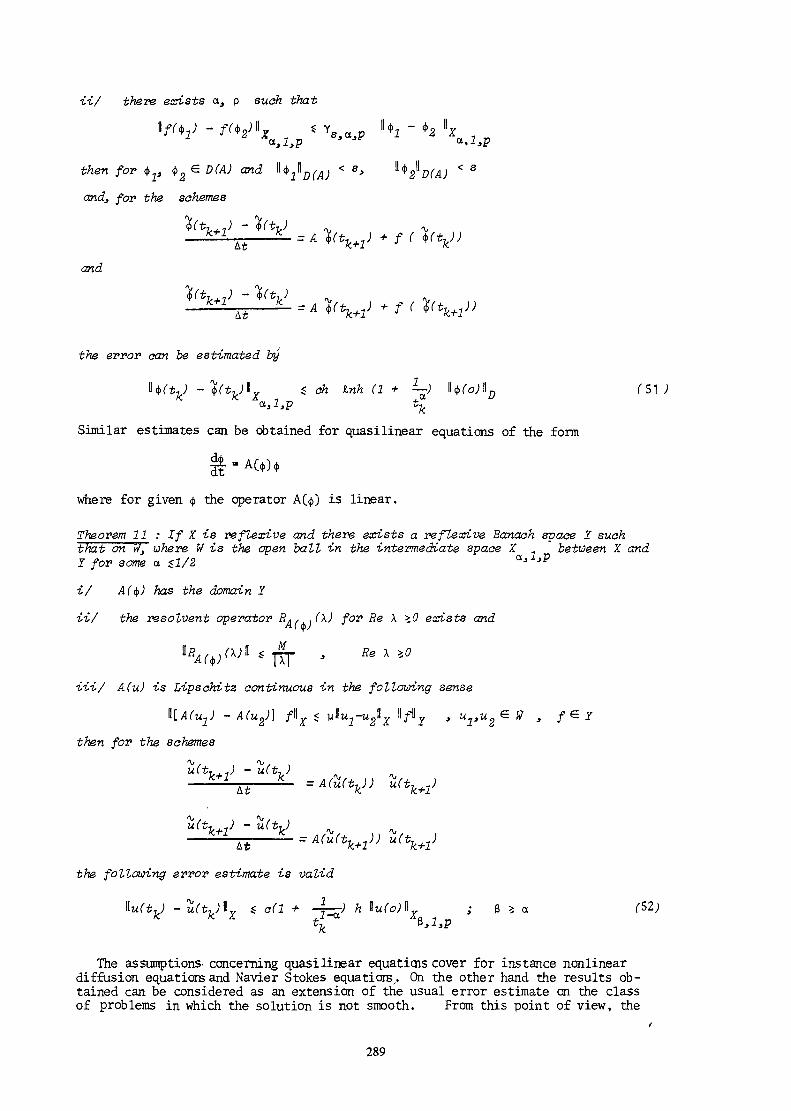
ii/ there exists o, p such that

then for 4,^ <j>2 € D (A) and l*J>D(A) < s>

and, for the schemes

and

the error can be estimated by

( s i ;

Similar estimates can be obtained for quasilinear equations of the form

where for given <j> the operator A(<j>) is linear.

Theorem 11 : If X is reflexive and there exists a reflexive Banach space I suchthat on J/, where W is the open ball in the intermediate space X between X and2 for some a $2/2

•i/ A($) has the domain Y

ii/ the resolvent operator A / / . i(M for Re \ >0 exists and

Hi/ A(u) is Lipschitz continuous in the following sense

ft[A(u2) - A(u2)} flly $ M\\UI-U^X \\f\\y , u2,u2 S W } f

then for the schemes*\j r\ju(tk ) - u(tk)

t

•= A(»<*» »At k+l

the following error estimate is valid

~ h u(o)^ ; ß a

The assumptions- concerning quasilinear equations cover for instance nonlineardiffusion equations and Navier Stokes equation? „. On the other hand the results ob-tained can be considered as an extension of the usual error estimate on the classof problems in which the solution is not smooth. From this point of view, the

289

results are interesting not only for the reactor dynamics but are also significantfrom the point of view of the general analysis of the approximate methods. Theprocedure developed in [22, 26, 27, 28] can be considered as a basis for developingthe compact theory of the approximate method for evolution equation. Some of theerror estimates obtained in the above references are optimal in the sense that theclass of the initial states for which the estimate is valid can be defined.

2.5. The generalized quasistatic method [133 [ 20l

fluxThe point of departure is ±he following alternate décomposition of the vector,., T _ r j. rZ. 4.^ j. rZ. 4. M 1(?,t)]

Kr,t)T(t) =TG(t)

Kr.t)0 *G(r,t)

= T(tWr,t) (53 )

The left hand decomposition is used for the "amplitude" equations, the right handdecomposition for the "shape" equations. The usual quasistatic method [ 29] is gene-ralized by allowing for G different amplitudes instead of a single one for everygroup. The factorization is made unique by imposing G conditions :

*g(r) v~%g(r,t)dï = 1=1,...G (54)

where $ (r) is the normalized critical adjoint flux in group g with velocity v .& o

Using (2) with u(t) = e where n is a constant diagonal matrix, N(t) =0, a = 1and allowing for the source Q(t) we have to solve a system of tyne

h h[I - / £2Ct)dt [A(h)-n H|(h) = exp(flh) [I + / £, (t)dt{ A(o)-fi]]|(o) + 3 ( 5 5 )

By proper choice of n, f- and f~ we can allow for spectral matching. The eigen-values are interpolated linearly.

Two time scales are used : the macrostep h., used for the shape equations areintegral multiples of the microstep h used for the amplitude equations .The spatial dependence of the flux ana precursors shape functions is given by afinite element formalism [ 30] . The reactor domain is partitioned in elementary rec-tangular subdomains e. . In each domain e. , any function u(r) reduces to a functionu (r) whose behaviour is local

Ni= S ( 5 6 )

The basis functions u.(r) obey the cardinality condition u. Ov) = <5? and areelements of the LagraAge basis associated to the unknowns -1 $..The u-(r) are polynomials of degree (k-1) containing at least-1 all monomials xpyq,p+q ^k-1, kg 4. The system of unknowns ( j> . is obtained by a Ritz-Galerkin method.

The critical steady state flux and adjoint flux are obtained by a power iterationcombined with Chebyshev extrapolation. Rebalancing factors are used. Finally thealgorithm amounts to the repeated solution of one-group problems with source solvedby a direct inversion obtained by a Cholesky factorization.

The integration procedure for the point kinetics equations uses an extrapolationprocedure derived from the Bulirsh-Stoer method [ 311 . Let T(t,h) be the solutionof an amplitude equation obtained by a convergent discretization with microstep h :

mT(t,h) = T(t) = S Ti(t) h x + (57)

290

Yv PmC h )

Let R (hT) = ——— , y = 1 or 2, be a rational function of h' A the degree of poly-Qm(h-Y) nomials P and Q being respectively u = [ -j \ and m-v . If the

amplitude equations are solved for a set of time steps { h - } , it is possible to cons-truct a rational function Rm(hY) such that Rm(hY) = T(t,h-J with t a point of themicrostep grid. An optimal sequence is obtainea by h- = n/n^, where for instancen-=1,2,3, n.+1 = 2n. ,. Not only very accurate values can be obtained for T(t,o)but the algorithms ^give also upper and lower bounds for the solution. Proceduresfor stepsize reductions stem from the same algorithm.

The system resulting from (55 ), where we have substituted (53 ) , is decompo-sed into four nonlinear subsystems : flux shapes, precursors shapes, flux amplitudes,precursors amplitudes,Nonlinearity stems for the product of shape and amplitudeunknowns. The amplitude functions are solutions of a system of (I+1)G differentialequations so called "multipoint kinetics", whe_re I is the number of precursors and Gthe number of groups. To solve such system F(x) = 0 in a consistent way, we shoulduse a Newton-SOR type algorithm [32] :

where F1 (x ) is the Frechet derivative of F for the m iterate. As usual a modi-fied Newton method is substituted. The main numerical task is the solution of asystem of type :

where •£ .. (nh) is the m+1 iterate of the "shape function" vector at macrostep nhand K ,"¥ the destruction and fission operators defined in eq. (7) and evaluatedat iteration m.

Problem (59 ) is quasisingular. The constraints (54 ) may prove incompatiblewith the unique solution of (59 ) . Compatibility must be restored by the additionof new degrees of freedom. We sketch below [ 34 ] the method used for G=1 (andwhich can be generalized for arbitrary G [13]) and which can be used in many ins-tances where we have to "solve" approximations of Boltzmann equations with cons-traints .We tackle the problem in a new manner different from previous ones [ 35] [ 36] , whichpreserves the normalization at each iteration step and yielding a convergence crite-rion. We formulate the problem as :

(M - oil - XF)i|) = Q (60 )

{ <f.i|> E <W,<|)> =1 (61 )

with either u or A as a "pseudoeigenvalue" . We choose here to find X. We adopt herethe technique of ANSELONE and RAIL [37] . Let S denote the field of complex numbersand X a Banach space which contains the domain of M - «I - F. Consider Y = X S S =COM)! * € X,X e S} with B Of;, A) II = max CM , ) x | ) .

We define G, application of Y into itself :GOO = GU,X) = ( [ M - ul - xFU - Q,

The solution of the nonlinear equation G = 0 is given by the modified Newton method

with

(I - çv<t,)K"1 çv

with K = M - (ul, v = K F'j), Çifrv = 1 .291

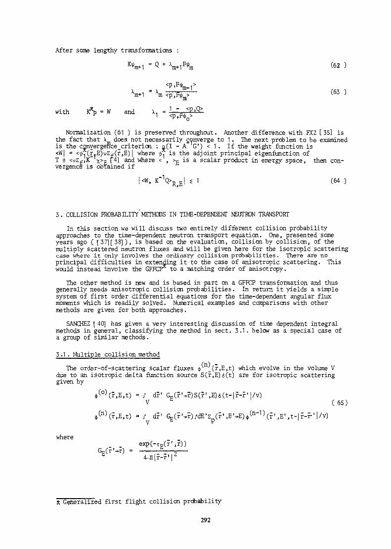
After some lengthy transformations :

(62

xm (-63

with K*p = W and*

Normalization (61 ) is preserved throughout. Another difference with FX2 [35] isthe fact that \ does not necessarily converge to 1. The next problem to be examinedis the conyergehce_criterion : o(I - A G') < 1 . If the weight function is<W| = <i|/.j (r,E)v2£(r,E) | where $- is the adjoint principal eigenfunction ofT = <v2£,K~ x>g f4] and where < , >E is a scalar product in energy space, then con-vergence is obtained if

|<W, K ' 1 Q > | < 1 (64 )

3 , COLLISION PROBABILITY METHODS IN TIME -DEPENDENT NEUTRON TRANSPORT

In this section we will discuss two entirely different collision probabilityapproaches to the time-dependent neutron transport equation. One, presented someyears ago ( [37] [38]) , is based on the evaluation, collision by collision, of themultiply scattered neutron fluxes and will be given here for the isotropic scatteringcase where it only involves the ordinary collision probabilities. There are noprincipal difficulties in extending it to the case of anisotropic scattering. Thiswould instead involve the GFFC^ to a matching order of anisotropy.

The other method is new and is based in part on a GFFCP transformation and thusgenerally needs anisotropic collision probabilities. In return it yields a simplesystem of first order differential equations for the time-dependent angular fluxmoments which is readily solved. Numerical examples and comparisons with othermethods are given for both approaches .

SANCHEZ [ 40] has given a very interesting discussion of time dependent integralmethods in general, classifying the method in sect. 3.1. below as a special case ofa group of similar methods .

5.1 . Multiple collision method

The order-of -scattering scalar fluxes $ _(r,E,t) which evolve in the volume Vdue to an isotropic delta function source S(r,E)i$(t) are for isotropic scatteringgiven by

= / dr1 G-Cr'-^SCr'.QsCt-lf-r ' /v)V ( 6 5 )

=/ dr1 Gp(?'*ï);dEfï (?' .EVE)^11"^ (?' ,E' ,t-|r-r' /v)y c P

whereexp(-TE(r',r))

4,n|r-r'

* Generalized first flight collision probability

292

The total neutron flux is the sum of the collision generation fluxes according toKr,E,t) -S *(n)(r,E,t)n=o

In the flat flux CP approximation Eq$. ( 65 ) yield in component form

XT C1,Cn) _ s pg c rgg'cS=1 Pij S( Cj S

where <j>; is the n:th collided flux in region i, group g and time bin m,

P|. are the ordinary collision probabilities

£jgg - £5? A-g scattering plus fission probabilities for energy transfer1 P & from group g' to group g (these probabilities are of theadjoint type and appear when we solve the flux rather thanthe collision density) .

The quantities e|.(m',m) are included to account formally for the time dependence.Their physical meaning can be described in the following way : consider neutrons intime bin m1 that have just suffered their n:th collision in region j being emittedin energy group g. Then P?.e?. (m',m) is the fraction of these neutrons that reachregion i, without further collision, at a time belonging to the time bin m. Thee:s depend upon several factors, namely :- the average time-of-f light , T? • , for neutrons in group g from their birth in re-gion j to first collision in region i,

- the time bin structure t = o, t^, to. ..t..- the strategy used for overlapping the sui- the strategy used for overlapping the successively scattered fluxes.

There is no unique definition of the flight time T?-. However, in the presentCP formulation it is natural to take •*

v/ dr 2? v/ dr'G (r'•+•?) | r-r ' |T§ = -*—————Î———-———————

Vg Vj Pij

where the average flight distance from uniform neutron birth in region j to firstcollision in region i is calculated using collision probability weighting. Definedin this way, the first flight collision time (ETC!) matrix Te also has the physi-cally desirable property of being symmetric.The idea of using mean flight times for time-dependent neutron transport has also beendiscussed by d'OULTKEMQNT [ 41] and d'OULTREMONT"and YOUNG [ 42] .

From their definition it is evident that the s:s will satisfy the following gene-ral conditions :

i/ S e|-(m*,m) = 1 to ensure neutron conservation

ii/ efjOn',nO = eÔn' »m) since Tg is symmetric and

iii/ e|.Cm',m) = 0 when m' > m

293

The overlapping problem arising when going from one collision generation to thenext is illustrated in Fig. 5. Neutrons coming out of the n:th collision in regionj, energy group g and time bin m' have a time-of-f light T?. to region i. If, aftera translation T?., the time interval At , = (tmt_i>t ) is-1 disjunct with or fallsentirely within at , the scoring in At is obvious and we will have e?-(m' ,m) equalto 0 or 1, respectively. -1

However, in the case shown in Fig. 5 we will have to define a way of dividing thescattered contribution between At and, say, At , . This must be based on an as-sumption of how the arrival times are distributes for group g neutrons going betweenregions j and i. In LEFVERT ([37] [38]) it was simply assumed that this distribu-tion is uniform and adding the assumption that the width of the time bins neverdecreases as a function of time (this is no restriction in practice but simplifiesthe overlapping calculation since now the overlap can never affect more than twoneighbouring time bins) , we may define the overlapping according to

1 - s| .. (m1 ,m)

(66)

It is easy to see that Eqs. ( 6 6 ) satisfy the general conditions i/-iii/ above.

Applications with the above method has shown very good agreement with time de-pendent S and Monte-Carlo calculations for systems that are scattering dominated.When absorption dominates,, the assumption of a uniform distribution of arrival timesfor neutrons travelling from one region to another is no longer sufficient.

Finally we discuss one more example from the same reference, where the multiplescattering method was used to analyze a pulsed neutron experiment by GOZANI [ 43] ona depleted uranium sphere. The U content was only 0.2 \ but the presence of thissmall amount manifests itself when we look at the U fast fission response,5whichafter 30 s is dominated by the build-up of slower neutrons which fission U andfeed the fast population. This very high sensitivity is very interesting for safe-guards purposes.

5 .2 . A time dependent neutron transport method

A- Theory

The starting point for the derivation of this method is the time dependent inte-gral transport equation for the angular neutron flux

<j>(r,E,a,t) = / dr'/dn' G(r' ,5'->-r,n) [Q(r' ,E,n' ,t- |r-

+ /dE'/dß"z (.T',E'-*E,a*+a'')<k(T' ,E,ä",t- r-r'l/v)]PIf we perform a Laplace transformation of this equation with respect to time, we get

(67)+ /dE'/do" 2fr',E'->£,f2"-H

where $ and Q are the Laplace transforms of the flux and source, respectively, and thenew kernel is

exp [- TF(r,r') - |r-r'| p/v]Ge(r',n '-*•?,«) = _ _ 2|r-r'|294

where n = (r-r')/|r-r'| and T-p(r,r') is the optical path length between r and r'.O IjThe GFPCP method applied to Eq. (67) yields, in analogy with the stationary case

discussed by LEFVERT [ 44] , in matrix form

= A ( p ) ( 6 8 )

The next step is to express the implicit GFFCP matrix A (p) in terms of the trueGFFCP matrix of the system according to the transformation law of TAKAHASHI [ 39]

A 00 = (I +

where I is the unit matrix.After rearrangement

PAV~V1 A

pv-1 .-1.

which gives the following system of equations for the time dependent angular momentsof the neutron density n = v $

s- -1 )vn + Q(t) + n(o)6(t)) (69 )

As mentioned by TAKAHASHI [39] the GFFCP transformation is exact, within the flatflux approximation, only when A is infinite. A differential equation oftype(68) with a finite order Legendre expansion of the angular flux does not predictwave propagation of uncoilided neutrons.But with the information given in the coefficient matrix of Eq. (69 ) the solutionwill try to simulate zero neutron density when the neutrons have not yet arrived.Numerically this is manifested, if the, order of anisotropy is greater than zero, innon-physical behaviour with fluctuations and negative neutron densities up to thetime when neutrons can be present and the solution stabilizes. This problem can beavoided either by simply disregarding the first part of the solution or start from ananalytical first collision source, as is often done in the S -method.

B. Numerical resultsThe first application is a homogeneous, infinite, one-group slab of thickness

2.5542 mfp (the thickness chosen to coincide with one of slabs treated by CARLVIK[ 45] who used an exact method to calculate the decay constant eigenvalue). We dividethe slab into five subrogions with equal thickness and put a delta neutron source inone of the outer regions.

,(n-1)r-*iikt It)

Fig. 5 : Overlapping of successive collision generations295

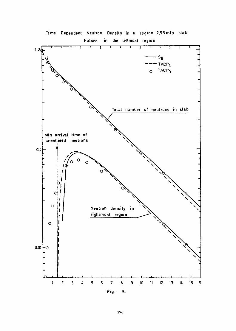
Time Dependent Neutron Density in a region 2.55mfp slab

Pulsed in the leftmost regioni i i T T i i T~ ' I T T | l "~

——— TACP4

o

0.1

Total number of neutrons in slab

Mir» arrival time ofuncollided neutrons

0.01

Neutron density inrightmost region

1 2 3 L 5 6 7 8 9 10 11 12 13 14 15 S

-O

296

Time Dependent Neutron Density for Group 3 Neutrons in aHeteregeneous Slab Pulsed at One End. With Group I Particles.

n/cnt

Pu-region (5)

source region (1 )

| Na

1• 1.5t ——— 1

Pu

0.925

Na

3.0

U

2.5

Fe

2.0cm

J_ l l l l t

50 100 150 ns

Fig. 7.

The neutron velocity is 1 cm/s. This pulsed problem was solved both with a timedependent 5 -method recently developed by SODEKBERG [ 46] (N.D.R. Inst.) and withthe presenr\]FFCP method. Some results are compared in Fig. 6. We know fromCARLVIK [45] that the asymptotic decay constant is a = - 0.217 s . The Sg- methodyields a = - 0.220 as the asymptotic slope of the neutron density curves wftile thetime dependent anisotropic collision probability (TACP) method predicts a = - 0.225in the P^-approximation and also in P^. To get better agreement for the decay cons-tant we would have to take smaller regions as shown in LEFVERT and SKOGLUND [ 47]where this slab required 9 regions and a P2-approximation to predict within 1 \in a stationary eigenvalue calculation witR the GFFCP method. We found that alsothe total number of neutrons left in the slab was practically the same in P, and P*while the neutron, density at the opposite side of the slab got a slightly betterrepresentation with P. than with P-. Returning to Fig. 6, we see that the total neu-tron leakage is evidently described rather well even in PQ while pulse propagationis not since P gives, just as does diffusion theory, a positive neutron densityeverywhere in the slab as soon as the source is released. The solution of Eq. (69 )in the P2 or P,-approximation showed a fluctuating negative and positive neutrondensity up to the time when the neutrons could physically be present after which thesolution was smooth.

297

Next we study a heterogeneous slab with three neutron groups. The slab is pulsedwith group 1 neutrons in the left outer region (Fe) . The system is slightly subcri-tical with an effective multiplication factor k = 0 .989 as determined by a stationaryGFFCP eigenvalue calculation. Some of the results of a TACP2 solution are shown inFig. 7, namely group three neutron densities in the two outer Fe regions and in thePu-region nearest to the source. We see that while from 60 ns on the neutron•density is the same in the two outer regions,the neutron population in the slab isnot in the fundamental mode as is also clearly shown by the density in the Pu-region.

As a matter of fact, when we looked at the instantaneous decav constant^ = jîn all regions and groups the different «:s did not merge into a coranonasymptotic value until 200 ns. Another interesting feature was the behaviour ofthe average cosine of the angular neutron density which showed a rapid equilibrationwith no transient effects after 80 ns.From the above numerical examples it seems that the TACP method gives a good des-cription of the neutron density in a pulsed system. Since it is based on the inte-gral transport equation the boundary conditions are properly handled and also theleakage. Being a flat flux CP method it would of course not be cost effective inlarge systems where diffusion theory is superior. Instead it should be used to ana-lyze time dependent effects in small, heterogeneous systems where good methods arerather scarce at present.The TACP method thus has the same field of application as the time dependent mul-tiple collision method discussed in section 3.1. above.Compared to this method the TACP approach is conceptually simpler, runs faster butneeds anisotropic collision probabilities even when scattering is isotropic and, aswe have seen, does not give an accurate description of the wave front of uncolHdedneutrons.

4. SINGULAR PERTURBATION METHOD

4.1 . IntroductionThe singular perturbation method is closely related to the reactor dynamics due

to the fact that the time constants characterizing the system of equations descri-bing the behaviour of neutrons differ from each other sometimes by several ordersof magnitude. There are many ways to overcome numerical difficulties induced bythat phenomenon, some of them were described in previous sections of this chapter.

The characteristic feature of singularly perturbed equations is that the asympto-tic expansion of the solution obtained by standard perturbation procedures is notuniformly convergent to the exact one so that special algorithms have to be employed.

The research work in the field of the singular perturbation was devoted to threemain topics :a. investigation of the initial value problem for evolution equations in Banach

spaces ;b. application of the singular perturbation method to reactor dynamics;c. utilization of the singular perturbation method for investigating the asymptotic

properties of equations approximating the transport equation.The results obtained so far in frames of the CRP clearly demonstrate that the

singular perturbation method is a convenient tool for both numerical and mathema-tical analysis of the equations of reactor physics and should be further developed.

298

4.2. Singularly perturbed evolution equations in Banach spaces

The analysis of evolution equations containing small parameters multiplyingtime derivatives in Banach spaces has been motivated by the fact that the transportequation supplemented by the equations for the concentration of delayed neutronprecursors form a system of evolution equations.

Singularly perturbed evolution equations in Banach spaces were first consideredby KREIN [ 48 ] who analyzed the zeroth order aysmptotic expansion of the solutionto the single evolution equation by using three types of expansions : outer, innerand intermediate. The results of KREIN were extended to higher order approximationsand to systems of evolution equations by MIKA in a series of papers [ 49 - 53 ] .The characteristic feature of the algorithm applied by MIKA was the use of only twotypes of expansion : outer and inner. The necessary matching of the two is notaccomplished through the initial conditions.

4.3. Application of singular perturbation method to reactor dynamics

The singular perturbation method has been known in reactor physics as the promptjump approximation consisting in truncating the outer asymptotic expansion at thezero order term and neglecting the inner expansion completely. GOLDSTEIN and SHOTKIN[ 54 ] tried to extend the prompt jump approximation to higer orders but their re-sults based upon the intuitive derivation are valid only for the first order. Thesystematic application of the singular perturbation method to reactor kinetics wasfirst proposed by HENDRY and BELL [ 55 ]who derived the algorithm including theintermediate expansion by a purely heuristic argument.

The applicability of the singular perturbation method based upon the algorithmdeveloped in [ 53] to reactor kinetics"was analyzed from the mathematical point ofview by MIKA [56, 57 ]. The results of practical calculations for the one-pointreactor kinetics [ 58, 59 ] showed that the method is quite attractive, at least forthe one-point or nodal models, for both fast and thermal reactors.

As concerns the reactor dynamics the applicability of the singular perturbationmethod to the one-point reactor dynamics model with the instantaneous power feed-back or with the linear temperature feedback was demonstrated by MIKA [ 60 ] .The numerical program based upon the asymptotic expansion algorithm for solving one-dimensional reactor dynamics equations is under preparation [ 61 ] . It is hoped,on the basis of the experience gained up to now, that the program will be applica-ble for fast on-line dynamics calculations.

4.4. Asymptotic properties of the approximate model of the transport equation

The primary application of the singular perturbation, method is to supply a con-venient tool for solving numerically equations containing small parameters. Howe-ver, the method may be also used to derive from a given equation its approximatemodels and to analyze their asymptotic validity. A great deal of the researchcarried out in frames of the CRP was devoted to this subject and, in particular, tothe analysis of the asymptotic relationship between the transport equation and thediffusion equation. The analysis, included in [62-64] ,was based on the asymptoticexpansion algorithm similar to that introduced by Hubert in the kinetic theoryof gases.

In [ 65 ] it was demonstrated that the diffusion equation and the equations obtainedin the first order spherical harmonics approximations are asymptotically equivalentin the sense that the neutron density calculated from both approximations tend toeach other as a square root of the quantity roughly proportional to the ratio of theabsorption and scattering cross sections.

5. NONLINEAR REACTOR DYNAMICS

Nonlinear reactor stability problems have been studied in the framework of nodaldynamics, which is felt to be a flexible and relatively unexpensive tool for suchinvestigations when space-dependence of perturbations or feedbacks is important.

299

A two-node kinetic model with constant power coefficients, K., and arbitrary delaytimes, r . - , in the neutronic coupling, e - - , between nodes i, j nas first been consi-dered [ ôè-1] . The advancement with respect to previous treatments [ 67] [ 68 ] concernsmainly the nonlinear stability conditions (in a parameter space) and the determina-tion of the admissible perturbations (region of attraction in a state space) in thecase when the reactivity feedback is positive in one node, as for a reactor with alocal positive reactivity feedback.

A more general method applicable to an n-node reactor model, n ^ 2, was thendeveloped [69] [ 70 ] . With respect to previous nodal stability treatments, thismethod

a) relaxes many restrictions (n = 2, K- ¥ 0 i, r.. = r . . , e. . = e.. no longer requi-red); x ^ 3i iJ 3i

b) determines a nonlinear stability condition in a parameter space which is in noway affected by the delays r.., even if some K. < 0 ;

c) the destabilizing effect of delays induces only a reduction in the region ofattraction u, which is constructed in the state space of the relative excess nodalpowers, x.;

d) stability for all physically significant perturbations (x. > -1 ¥i) is ensured forany delays r.. 5 0, if all nodes show a stabilizing feedback C <• > 0 "^ i)•

For the case of variable (power-dependent) power coefficients the two-node problemwith arbitrary r^• was first treated [ 71 I . The region of attraction has been rela-ted to the functional dependence of nodal feedbacks on Dowers, in both cases that suchregion does or does not contain all physically significant perturbations.

The problem of a two-node reactor with power and temperature feedbacks representedby constant coefficients has also been treated [ 72 1 . All physically significantperturbations are shown to be in the region of attraction of the operating equili-brium state, even with destabilizing temperature feedbacks, provided each power feed-back is stabilizing and sufficiently large. In other important cases an appropriateregion of attraction has been determined.

A more general theory of nonlinear stability for systems with positive statevectors (i.e. for which physically significant values of suitably defined statevariables are positive) has been then worked out, with the purpose of obtaining ge-neral results applicable to stability problems for n-nodes reactor systems dynamics[73] with variable power coefficients. Stability conditions determined in the caseof constant coefficients were confirmed in this more general context. The introduc-tion of a Lyapunov function composed by the union of 2 suitably connected quadra-tic functions offered a considerable extension of all previously estimated regionsof attraction of the operating equilibrium state. The new estimates are the unionof 2n hyperelliptical regions.

REFERENCES

[1] J. DEVOOGHT, E. MUND in Proceedings of the Joint NEACRP/CSNI Socialists'Meeting on New Developments in 3D Neutron Kinetics and Review of KineticsBenchmark Calculations", T.IT. München, Garching 1975.

[21 H. STETTER, "Analysis of discretization methods for ordinary differentialequations", Springer, 1973".

[3l G.G. DAHLQUIST, BIT 3_, 27-43 (1963).

[41 R.S. VARGA, "Matrix iterative analysis", Prentice Hall, New Jersey (1965).

[51 A.F. HENRY, Nucl. Sei. Eng., 20t, 338 (1964).

[61 J. MIKA, Report INR 700/XXI, RP (1966).

300

t 71 T. FORSCHUNG, SIAM J. Aüpl. Math, 1_6_, 301 (1968).

[81 T. KATO,'Perturbation Theory for Linear Operators", p. 244, Springer (1966).

[9l J.L. WALSH, "Interpolation and approximation bv rational functions inthe complex domain'', Amer. Math. Soc. Coll. Publ., Vol. XX,N.Y. (1955).

i[101 J. DEVOOGHT, "The generation of A-stable approximations for the integration

of the Cauchy equation", Internal report, ULB.

[111 W. LINKER, R. WILLOUGHBY, SIAM J. Numer. Anal. 7_, 47-66 (1970).

[121 S. N0RSETT, BIT, J4_, 63-77 (1974).

[ 131 J. DEVOOGHT, E. MUND and a]. "Developments of New Numerical Methods forSpace-Dependent Nuclear Reactor Dynamics", EEC-DGIII - F2/TTLB Contract,Vols 1-3 (1977).

[14l R. STANKIEWICZ, New Chebyshev Rational approximation to evolution equa-tion, Report research contract N° 1236/RB" App. 37.

[151 W.J. CODY, MEINARDUS, R.S. VARGA, J. Approx. Th. 2_, 50-65 (1969).

[16] C.W. GEAR, The Automatic Integration of Ordinary Differential Equations,Comm. of ACM, Vol. 14, 1971.

[171 R. STANKIEWICZ, H.J. TOMECKI, Application of multisteu method in solvingthe one-point reactor dynamics model with feedbacks, Report R.C. N° 1236/RBApp. 46.

[181 J.C. BUTCHER, Maths, of Comp. U_, 50-64 (1964).

[191 C.W. GEAR, BIT 1_0, 20-22 (1970).

[201 M. BARDIAUX, J. DEVOOGHT, P. DUGNOILLE, M. GOLDWASSER, J. JOLY, E. MIND,I. SARAGOSSI, A. SIEBERTZ, "CASSANDRE : a 2D multigroun diffusion bench-mark code for fast reactors power excursions analysis", Proceedings of theENS/ANS Topical Meeting on Nuclear Power Reactor Safety, Brussels, October1978.

[21] J. DEVOOGHT, A. JAUCOT, C. MACHGEELS, in Proceddings of the Seminar onNumerical Reactor Calculations, IAEA, Vienna (1972) .

[22] R. STANKIEWICZ, On the rational approximation to the evolution equation,Report R.C. N° 1236/RB App. 38.

[231 R. STANKIEWICZ, Finite difference approximation to abstract parabolicequation in Banach space, Report R.C. N° 1236/RB App. 47.

[24] R.A. ADAMS, "Sobolev Spaces", Academic Press, 1975, N.Y., San Francisco,London.

[25] P.L. BUTZER, H. BERBMS, "Semigroup of Operators and Approximation"

[26] R. STANKIEWICZ, Finite difference approximation to temporal inhomogeneousparabolic equation, Report R.C. N° 1236 App. 4.

[27] R. STANKIEWICZ, Finite difference approximation to certain class of non-linear parabolic equation in Banach space, Report R.C. 1236 App. 49.

[28] R. STANKIEWICZ, Finite difference approximation to parabolic with non-linear perturbation, Report R.C. 1236 App. 5.

[29] K. OTT, D.A. MENELEY, Nucl. Sc. Eng. 36, 402 (1969).

301

[30] J.P. HENNART, E. MUND, Miel. Se. Eng. 62_, 55-68 (1975).

[31] R. BULIRSCH, J. STOER, Numer. Math. 8_, 1-13 (1966).

[32] J. ORTEGA, W. RHEINBOIDT, Iterative solutions of nonlinear equations inseveral variables, Academic Press, N.Y. (1970)".——————————————

[33] J. DEVOOGHT, "Spectrum of the multigroup-multipoint diffusion operatorwith delayed neutrons", Nucl. Sc. Eng. 67_, 147-161 (1978).

[34] J. DEVOOGHT, "Solutions of quasisingular problems with constraints arisingin quasistatic approximations", Proceedings of the ANS Topical Meeting onComputational methods in nuclear engineering, Williamsburg, April 1979.

[35] D.R. FERGUSON et al., "FX2, A quasistatic multidimensional-multigroupdiffusion theory code with feedback", FRA Tech. Memo 87 (1976) .

[36] D.E. BILLINGTON in [ 1] .

[37] P. ANSELONE, L. RALL, Numer. Math. Jj_, 38-45 (1968).

[38] LEFVERT T., Proc. Conf. Computational Methods in Nucl. Engineering,CONF-750413, Vol. II (1975).

[39] TAKAHASHI H., Nucl. Sei. Eng. 26, 254 (1966).

[40] SANCHEZ R., Unpublished notes, Dep. Nucl. Eng. Univ. of Washington,Seattle, Wash., USA (1977).

[41] d'OULTREMONT P., Nucl. Sei. Eng. 37_, 104 (1969).

[42] d'OULTREMONT P. and YOUNG J.C., ibid. 40, 338 (1970).

[43] GOZANI T., Nucl. Sei. Eng. 36_, 143 (1969).

GOZANI T. and d'OULTREMONT P., Trans. Amer. Nucl. Soc. 1_2_, 258 (1969).

[44] LEFVERT T., Nucl. Sei. Eng. 54, 369 (1974)."A Collision Probability MetEôd for Time Dependent Neutron Transport",FOA C 20017-A2, Nat. Defence Res. Inst., Stockholm, Sweden (1974).

[4SI CARLVIK I., Nucl. Sei. Eng. 3_1_, 295 (1968).

GOPINATH D.V., "Integral Equation Methods in Radiation Transport", NBSSpec. Pufal. 461, Proc. of Int. Symp. on Radiation Physics, National Bureauof Standards, USA.

[46] SODERBERG S., "NTR1 - A computer program for time dependent neutron trans-port in plane and spherical geometry", forthcoming FOA-report (in Swedish),National Defence Research Inst. Stockholm, Sweden (1979) .

[471 LEFVERT T. and SKOGLUND R., "Calculations of the Neutron Decay Constantin Slab Geometry Using Anisotropie Collision Probabilities", FOA C 20176-A2,Nat. Defence Res. Inst., Stockholm, Sweden.

[481 KREIN S.Gv, "Linear Differential Equations in Banach space", AmericanMathematical Society, Providence, R.I., 1971.

[491 MIKA J., Mathematica Balcanica 3_, 321 (1973).

[501 MIKA J., Joum. Math. Phys. 15_, 892 (1974).

[511 MIKA J., Annales Polonici Math., 32., 43 (1976).

[ 52] MIKA J., Singular perturbation method for evolution equations in Banachspaces, in "Mathematical Physics and Physical Mathematics", K. Maurin andR. Raczka, eds., PWN-D.Reidel, Warsaw 1976, p. 263.

302

[53] MIKAJ. , Journ. Math. Anal. Appl. 58_, 189 (1977).

[541 R. GOLDSTEIN and L.M. SHOTKIN, Nucl. Sei. Eng., 38_, 94 (1969).

[55] HENDRY W.L. and BELL G.I., Nucl. Sei. Eng. 35_, 240 (1969) .

[ 561 MIKA J., Nukleonika 1£, 1013 (1975) .

[571 MIKAJ. , Nukleonika 21_, 573 (1976).

[581 BLENSKI T., GADOMSKI A. and MIKA J., Nucl. Sei. Eng. 66, 277 (1978).

[591 BLENSKI T., Atomkernenergie 31_, 232 (1978).

[60] MIKA J., Application to the singular perturbation method to reactor dyna-mics equations, Internal report.

[ 61] GADGMSKI A., Application of singular perturbation method to numericalsolutions of one-dimensional nonlinear reactor dynamics equations,Internal report.

[62] MIKAJ. , Nukleonika 23_, 221 (1978).

[63] MIKA J., Hubert asymptotic expansion method for the linear Boltzmannequation, in "Fundamental Problem in Statistical Mechanics IV", E.G.D.Cohen and W. Fiszdon, eds. Zaklad Narodowy Ossolinskich, Wroclaw 1978.

[641 MIKA J., Asymptotic methods for singularly perturbed linear differentialequations in Banach spaces, in "Equadiff IV, Proceedings", J. Fabera, ed.Springer Verlag, Berlin 1979.

[651 MIKA J. and STANKIEWICZ R., Transport Theory and Statistical Physics, 7(3), 81 (1978).

[ 66] BARAN W. and TROMBETTI T., "Estimating the domain of attraction of a stableequilibrium state for certain delayed differential systems of order two",Meccanica, 1J_, 3 (1976).

[671 WEAVER L.E., Reactor Dynamics and Control, American Eisevier, N.Y. (1968).

[68] NOLDUS E., 'The stability of coupled-core nuclear reactors", J. Eng. Math.,6_, 31 (1972).

[69] TROMBETTI T. "Reactor Stability in the Nodal Approximation", TransactionsANS, 21_, 481 (1975).

and

"Stabilita dell'equilibrio per sistemi differenziali con tempi di ritardoed accomppiamenti non negative", "Problemi di diffusione e propagazione",Quademo dei Gruppi di Ricerca Matematica del C.N.R., p. 135 (1975).

[701 BARAN W. and TROMBETTI T., "Recent Advancements in Nonlinear ReactorStability", Italian Contributions to I.A.E.A.'s Specialist Meeting on"Methods of Neutron Transport Theory and Reactor Calculations", Bologne,3-5 November 1975, Pitagora Ed.,Bologna.

[71] BARAN W. and TROMBETTI T., "Stability Problems for Second Order DelayedDifferential Systems with Variable Feedback Coefficients in Nuclear ReactorDynamics", Report RT/FIMA (76) 1, Comitato Nazionale per 1'Energia Nucleare,Rome, 1976.

[721 TROMBETTI T. and BARAN W., "Nonlinear System Stability and Applicationsto Two Node Nuclear Reactor Models with Power and Temperature Feedbacks",Report RT/FIMA (76)2, Comitato Nazionale per 1'Energia Nucleare, Rome,1976.

303

[73l TROMBETTI T., "Problem! di stabil!ta dell'equilibrio per sistemi a vettoridi stato positiv!", Paper 1-15 presented at the "III Congresso NazionaleA.I.M.E.T.A.", Cagliari, 13-16 ottobre 1976.

[741 DEVOOGHT J., Journal of Comp. and Appl. Math. 2_, 231-240 (1976) .

[75] DEVOOGHT J., MONO E., VAN VLIET J., VAN WYLICK J., Trans. Am. Nucl. Soc.r7_, 253 (1973).

[761 MUND E., VAN BINNEBEEK J.J., "Méthodes linéaires multipas et conservationspectrale", Colloque d'analyse numérique, Port-Bail (France) (1976) .

[77l MUND E., VAN BINNEBEEK J.J., 'linear multistep methods and spectral matching1

SIAM National Meeting, Chicago (1976) .

[78] MUND E., VAN BINNEBEEK J.J., Bull. Acad. Classe des Se., Ac. Royale deBelgique, Sème série, Tome LXII 289-311 (1976).

[79l MUND E., VAN BINNEBEEK J.J., "Properties and applications of a rationalinterpolation algorithm in the complex unit disk", Contact group NFWO-FNRS,Meeting on "Constructive methods in approximation theory", Brussels (1976).

[801 DEVCOGHT J., "Quasistatic solution of reactor kinetics", Internal report,ULB (1978).

304

Chapter VIIBENCHMARK PROBLEMS

A. KAVENOKY, J. STEPANEK, F. SCHMIDT

1. INTRODUCTIONThe benchmark organization had been considered to improve the

exchange of informations between the different teams working for thecoordinated research program and to make conspicuous the needs of improvedcalculation tools based on refined analytical methods.

Three groups of benchmarks had been proposed : the first group wasdecided at the Swierk (Poland) Coordination Meeting of the program [1973).This group of problems is based on one dimensional transport problems, it iscomposed of four problems that will be named Swierk 1 to 4. The results ofthese benchmarks has been reviewed at the Bologna (Italy) meeting (1973).

The second group of benchmarks was proposed after the Bolognameeting ; two benchmarks related to two-dimensional assembly-problems hadbeen proposed by France and are named CEA 1 and 2, Two other benchmarkstreat rectangular two-dimensional geometry and were provided by Switzerlandthey are named EIR 1 and 2.

These benchmarks had been reviewed a first time at the Parismeeting in 1977 but the results had not allowed to obtain a final conclusion ;a second review was done at Lugano in 1978 and definite conclusions wereobtained.

The detailed test of all these benchmarks are given in Annex.

2. BENCHMARK SWIERK-1This three-layer one energy group problem had been designed to

simulate the simplest slab reactor with one central multiplying region andtwo symmetrical reflecting zones.

For this benchmark a few results had been presented using variousprograms. ANISN [1] results were given by the Swiss team who performs alsocalculations using their own code SHERLOCK. [2] ; the integral transform method[3] was used by Italy and the point-wise collision probability method (CRN)[<+] was used by Yougoslavia.

The comparison of these given on Table 1 shows that the exactresult is known with at least five exact figures : the swiss, Italian andyougoslavian results converge to the same value.

The convergence of the results based on the integral equation isfaster than the convergence of the Sj\| method ; moreover the Legendrepolynomial expansion method provided fast and accurate results for thissimple problem.

3. BENCHMARK. SWIERK-2

This one slab benchmark is devoted to the calculation of theescape probability for a scattering, absorbing and eventually multiplyingslab in one velocity theory.

305

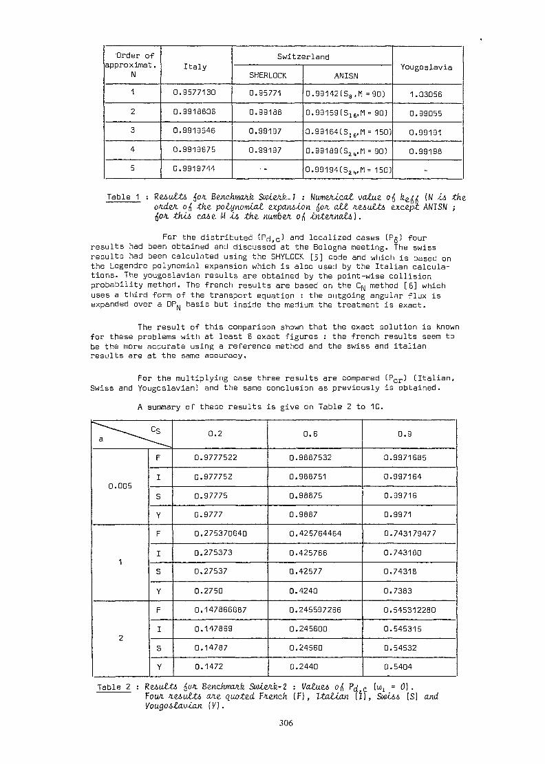
'Order ofapproximat .

N123

45

Italy

0.95771300.9918806

0.9919646

0.9919675

0.9919744

SwitzerlandSHERLOCK0.95771

0.99188

0.99197

0.99197

ANISN

0.99142(S8,M =90)

0.99159(S16,M = 90)

0.99164(S16,M= 150)

0.99189(S2I(,M = 90)

0.99194(S2VM= 150)

Yougoslavie

1.03056

0.99055

0.99191

0.99198-

Table 1 : ReAuLt& fou Be.nckmatik Sw4.znk.-1 : Mu.mMA.cat uo£tte ofi fee(j/ [N <i& the.oldest, o^ the. potynomiaJt e.x.panA<lon faon att fuLt>uLU> exce.p-t AWISN ;

M -a the. numoeA o& JijnX.ejinoJLt>\ .

Far the distributed (Pd,c^ and localized cases (Pg) fourresults had been obtained and discussed at the Bologna meeting. The swissresults had been calculated using the SHYLOCK. [5] code and which is based onthe Legendre polynomial expansion which is also used by the Italian calcula-tions. The yougoslavian results are obtained by the point -wise collisionprobability method. The french results are based on the C^ method [6] whichuses a third form of the transport equation : the outgoing angular flux isexpanded over a DP^ basis but inside the medium the treatment is exact.

The result of this comparison shown that the exact solution is knownfor these problems with at least 6 exact figures : the french results seem tobe the more accurate using a reference method and the swiss and italianresults are at the same accuracy,

For the multiplying case three results are compared CPcr) [Italian,Swiss and Yougoslavian) and the same conclusion as previously is obtained.

A summary of these results is give on Table 2 to 10.

" - csa ~~ ~ ^

0.005

1

2

F

I

S

YF

IS

YFIS

Y

0.2

0.9777522

0.977752

0.97775

0.9777

0.275370640

0.2753730.27537

0.2750

0.147866687

0.147869

0.14787

0.1472

0.6

0.9887532

0.988751

0.98875

0.9887

0.425764464

0.425766

0.42577

0,4240

0.245597266

0.245600

0.24560

0.2440

0.9

0.9971685

0.997164

0.99716

0.9971

0.743179477

0.7431800.74318

0.7383

0.545312280

0.545315

0.54532

0.5404

Table 2 : Reio&ti fan. Benchmark SwK.eAk-2 : Vatau, ofc ?^ cFoot. ïi&,uJt&> afii qaotid ¥ie.nch (F), Itatian (il,you.goAla.vULn [V].

(S) and

306

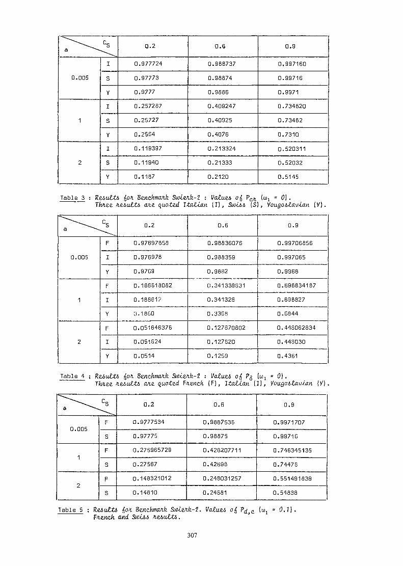
" \ csa \ _

0.005

1

2

I

S

YI

S

Yl

S

Y

0.2

0.977724

0.97773

0.9777

0.257267

0.25727

0.2564

0.119397

0.11940

0.1187

0.6

0.988737

0.98874

0.9886

0.409247

0.40925

0.4076

0.213324

0.21333

0.2120

0.9

0.997160

0.99716

0.9971

0.734820

0.73482

0.7310

0.520311

0.52032

0.5145

Table 3 :Tfet.ee

BencAma/ik. Sw-ceAfe-Z ; (/a£ue6one. quoted. 1ta£ia.n (T.],

0) .(S), (/)

^ \Csa --- ^

0.005

1

2

F

I

Y

F

I

Y

FI

Y

0.2

0.97697858

0.976978

0,9769

0.186618082

0.186612

0.1860

0.051646376

0.051624

0.0514

0.6

0.98836076

0.988359

0.9882

0.341338631

0.341326

0.3368

0.127670802

0.127620

0.1259

0.9

0.99706856

0.997065

0.9968

0.698834187

0.698827

0.6844

0.446062834

0.446030

0.4361

Table 4 ; SMM.e/ife-2 : Valu&> ofi P<$ (a^ = 0] .fiuuLU> (Vie. quot&d Ftencfc ( F ) , ItaJLian ( I ) , /oago4£av-ûiKi (V)

a ^ ^ ^

0.005

1

2

F

S

F

S

F

S

0.2

0.9777534

0.97775

0.275965729

0.27567

0.148321012

0.14810

0.6

0.9887536

0.98875

0.428207711

0.42698

0.248031257

0.24681

0,9

0.99717070.99716

0.746345135

0.74476

0.551491839

0.54838

Table 5 ; Re6u££ô faon Benchmark SiüteAk-2. faùteô ofaFterccfi and Sw/c64

* 0 .1) .

307

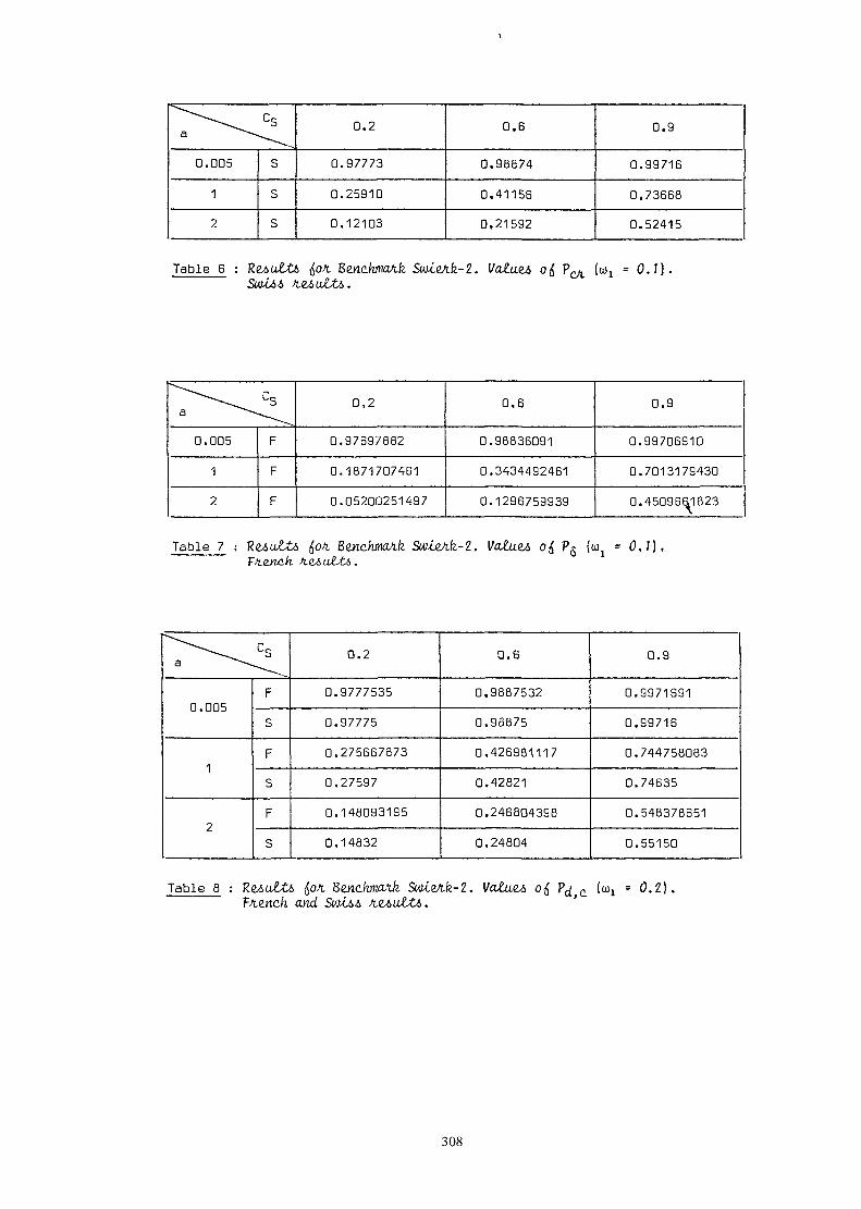
" \ csa ~~-~ ^ ^

0.005

1

2

S

S

s

0.2

0.97773

0.259100.12103

0.6

0.98874

0.411560,21592

0.9

0.99716

0.736680.52415

Table 6 : Swi.znk-2.. = 0.1}.

\ csa ~--- _ ^0.005

1

2

F

F

F

0.2

0.97697882

0.1871707461

0.05200251497

0.6

0.98836091

0.3434492461

0.1296759939

0.9

0.997069100.7013179430

0.4509661823

Table 7 ; Reiotti SuiieA.k-2. = 0 ,1 ] ,

^ - _ csa ^ ^ __

0.005

1

2

FS

FS

FS

0.2

0.9777535

0.97775

0.275667873

0.27597

0.148093195

0.14832

0.6

0.9887532

0.98875

0.4269811170,42821

0.246804398

0.24804

0.9

0.9971691

0,997160,744758083

0.74635

0.548378651

0.55150

Table a : R&iu&ti fan BencAmoA.fi Swte/tfe-2. VOULU ofa P^ c (<% = 0 .2) .F-tenc/i and Stocii - - - » - •

308

> ^0.005

1

2

S

S

s

0.2

0.97773

0.26095

0.12270

0.6

0.98874

0.41389

0.21857

0.9

0.99716

0.73854

0.52805

Table 9 ; Benchmark Sw-ceAfe-2. Value* (u1 = 0.2).

"\ csa "--- ^0.005

1

2

F

F

F

0,2

0.97697893

0.1877257844

0.05236196257

0,6

0.98836126

0,3455795994

0.1317252716

0.9

0.99707027

0.7038159343

0.4559528037

Table 10 : Reiutts ofi Benchmark. SwceAk-2. l/aCuwEtench

0 , 2 ) ,

4. BENCHMARK SWIERK-3

This benchmark is a simplified cell calculation in cylindricalgeometry and one-velocity approximation. Four results are composed for thiscase. Two results are provided by Switzerland one using the SHADOCK [7] code theother using the standard ANISN and two results are given by Yougoslavia oneby CRN and one by Monte Carlo calculation [8].

For the isotropic case the exact result may be close to 5560 : theresults that had been given do not allow more accuracy, The results are presentedon Table 11.

SHADOCK

ANISN - S8

CRN

MC

S

S

Y

Y

PO -°N1 = 3 5576,91

N' = 4 5562.78

5547.08N = 5 5521

N = 6 5558

N = 7 55565575

yfl - 0.2N' = 3 5013.50

N' = 4 5014.78

5010.54-

-_

-

Table mTtw 3loup& C($ tiuuZtb (Vie. piuented SWÄA& (S), y(W = numöeA ofi Aubie.g<ion& -in thé. mode/iatox. ; M

pointe, -en tke.

(Y)number,

309

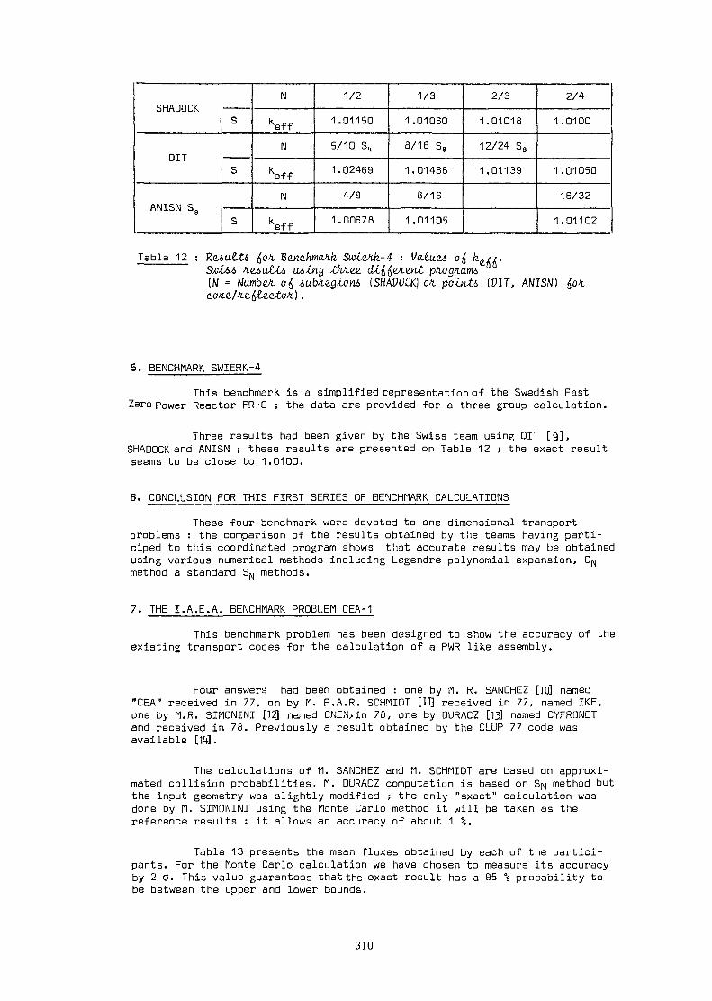
SHADOCK

DIT

ANISN S8

S

S

s

IM

KeffN

KeffN

Keff

1/2

1.01150

5/10 S„

1.02469

4/8

1.00678

1/3

1.01060

8/16 S81.01436

8/16

1.01105

2/3

1.01018

12/24 S81.01139

2/4

1.0100

1 .01050

16/32

1.01102

Table 12 :(N =

Re.nc.hmAk SuileJik-4 : l/o£cie4di^&L&n(SHAPÖCK) (PIT, ANISN)

5. BENCHMARK SWIERK-4

This benchmark is a simplified representation of the Swedish FastZero power Reactor FR-0 s the data are provided for a three group calculation.

Three results had been given by the Swiss team using DIT [9],SHADOCK. and ANISN ; these results are presented on Table 12 ; the exact resultseems to be close to 1.0100.

6. CONCLUSION FOR THIS FIRST SERIES OF BENCHMARK CALCULATIONS

These four benchmark were devoted to one dimensional transportproblems : the comparison of the results obtained by the teams having parti-ciped to this coordinated program shows that accurate results may be obtainedusing various numerical methods including Legendre polynomial expansion, Cpjmethod a standard S methods.

7. THE I.A.E.A. BENCHMARK PROBLEM CEA-1

This benchmark problem has been designed to show the accuracy of theexisting transport codes for the calculation of a PWR like assembly.

Four answers had been obtained : one by M. R. SANCHEZ [10] named"CEA" received in 77, on by M. F,A.R. SCHMIDT [1TJ received in 77, named IKE,one by M.R. SIMONINI [12] named CNEN,in 78, one by DURACZ [13 named CYFRONETand received in 78. Previously a result obtained by the CLUP 77 code wasavailable [14].

The calculations of M. SANCHEZ and M. SCHMIDT are based on approxi-mated collision probabilities, M. DURACZ computation is based on S^ method butthe input geometry was slightly modified ; the only "exact" calculation wasdone by M. SIMONINI using the Monte Carlo method it will be taken as thereference results : it allows an accuracy of about 1 %.

Table 13 presents the mean fluxes obtained by each of the partici-pants. For the Monte Carlo calculation we have chosen to measure its accuracyby 2 a. This value guarantees that the exact result has a 95 % probability tobe between the upper and lower bounds.

310

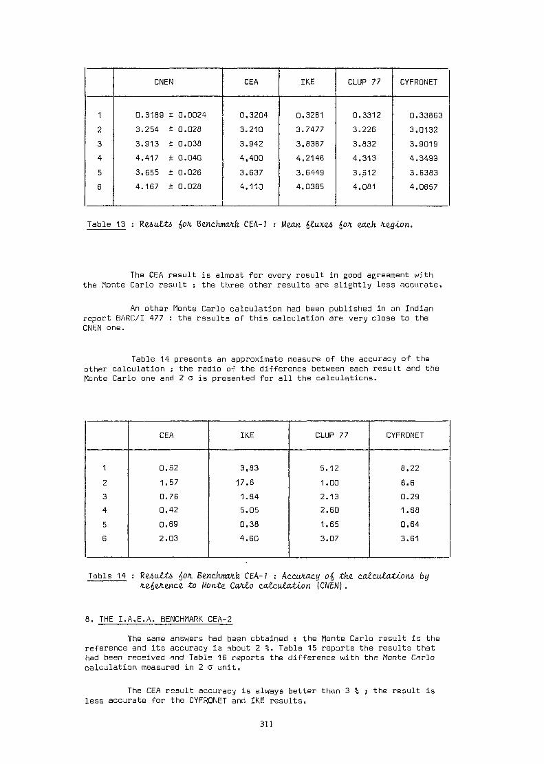
12345B

CNEN

0.3189 £ 0.00243.254 ± 0.0283.913 ± 0.0384.417 ± 0.0403.655 ± 0.0264.167 ± 0.028

CEA

0,32043.2103.9424.4003.6374.110

IKE

0.32813.74773,83874.21463.64494.0385

CLUP 77

0.33123.2263,8324.3133.6124.081

CYFRONET

0.338633.01323.90194.34993.63834.0657

Table 13 : Reiülti £01 Benchmark CEA-7 : Mean j$£u.x£4 ôn. each

The CEA result is almost for every result in good agreement withthe Honte Carlo result ; the three other results are slightly less accurate.

An other Monte Carlo calculation had been published in an Indianreport BARC/I 477 : the results of this calculation are very close to theCNEN one.

Table 14 presents an approximate measure of the accuracy of theother calculation ; the radio of the difference between each result and theMonte Carlo one and 2 a is presented for all the calculations.

12

3

4

5

6

CEA

0.62

1.57

0.76

0.42

0,69

2.03

IKE

3,83

17.6

1.94

5,05

0,38

4.60

CLUP 77

5.12

1.00

2.13

2.60

1.65

3.07

CYFRONET

8.22

8.6

0.29

1,68

0.64

3.61

Table 14 : Re4u££5 ôn Bencfc.maA.fe. CEA-7 : AccuAact/ otf the. calculation* byto Monte. Ca/ilo calculation (CNEN).

8. THE I.A.E.A. BENCHMARK CEA-2

The same answers had been obtained : the Monte Carlo result is thereference and its accuracy is about 2 %. Table 15 reports the results thathad been received and Table 16 reports the difference with the Monte Carlocalculation measured in 2 a unit.

The CEA result accuracy is always better than 3 % j the result isless accurate for the CYFRONET and IKE results,

311

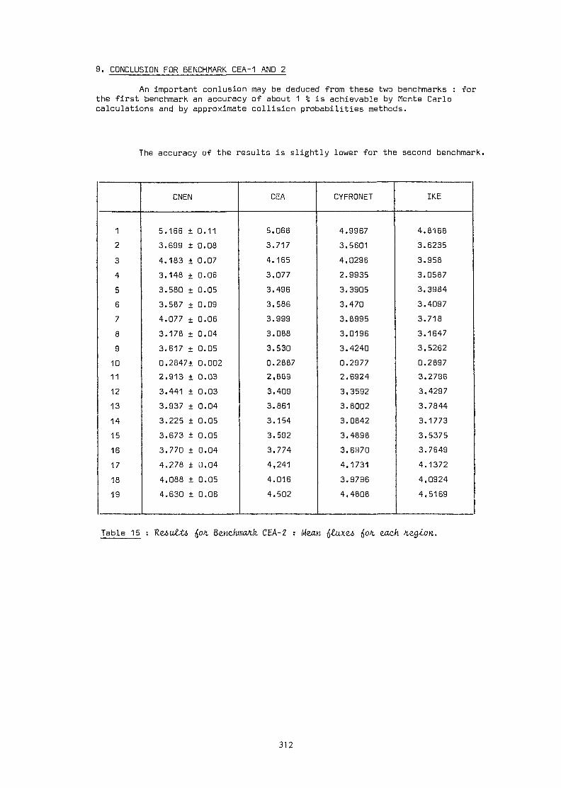
9. CONCLUSION FÜR BENCHMARK CEA-1 AND 2

An important conlusion may be deduced from these two benchmarks : forthe first benchmark an accuracy of about 1 % is achievable by Monte Carlocalculations and by approximate collision probabilities methods.

The accuracy of the results is slightly lower for the second benchmark.

12345678910111213141516171819

CNEN

5.166 ± 0.113.699 ± 0.084.183 ± 0.073.148 ± 0.063.580 ± 0.053.587 ± 0.094.077 ± 0.063.178 ± 0.043.617 ± 0.050.2847± 0.0022.913 ± 0.033.441 ± 0.033.937 ± 0.043.225 ± 0.053.673 ± 0.053.770 ± 0.044.278 ± 0.044.088 ± 0.054.630 ± 0,06

CEA

5.0683.7174.1653,0773.4963,5863.9993.0883.5300.28872,8893.4093.8613.1543.5923.7744,2414.0164.502

CYFRONET

4.99673,56014,02962.99353.39053.4703.89953.01963.42400.29772.69243,35923.60023.08423.48983.69704.17313.97964,4808

IKE

4.81683.62353.9583.05873.39843.40973.7183,16473.52620.28973.27963,42973.78443.17733.53753.76494.13724,09244.5169

Table 15 Benchmark CEA- 2 : Mean ôn. eacA .teg-con.

312

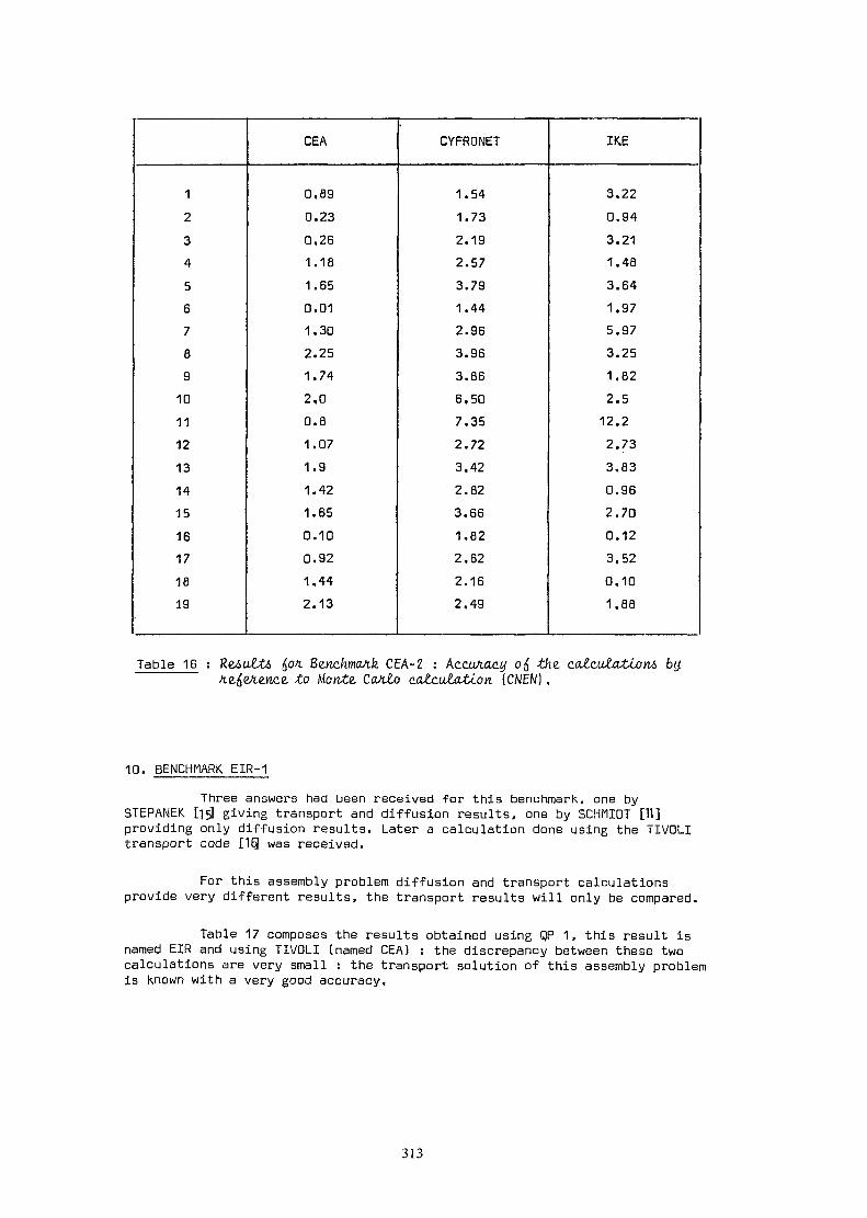
12345678910111213141516171819

CEA

0.890.230.261.181.650.011.302.251.742,00.81.071.91.421.650.100.921,442.13

CYFRONET

1.541.732.192.573.791.442.963.963.866.507.352.723,422.823.661.822.622.162.49

IKE

3.220.943.211.483.641.975.973.251.822.512.22.733.830.962.700,123.520,101.88

Table 16 : Re6u££6 {,01 Bercc.ftmcw.fe CEA-2 : Ac.cuAo.ct/ o£ the. calculation!* by.tie.&esience. to Monte. Canlo calculation ( C N E N ) ,

10. BENCHMARK EIR-1Three answers had been received for this benchmark., one by

STEPANEK [15] giving transport and diffusion results, one by SCHMIDT [11]providing only diffusion results. Later a calculation done using the TIVOLItransport code [16j was received.

For this assembly problem diffusion and transport calculationsprovide very different results, the transport results will only be compared.

Table 17 composes the results obtained using QP 1, this result isnamed EIR and using TIVOLI Cnamed CEA) : the discrepancy between these twocalculations are very small : the transport solution of this assembly problemis known with a very good accuracy.

313

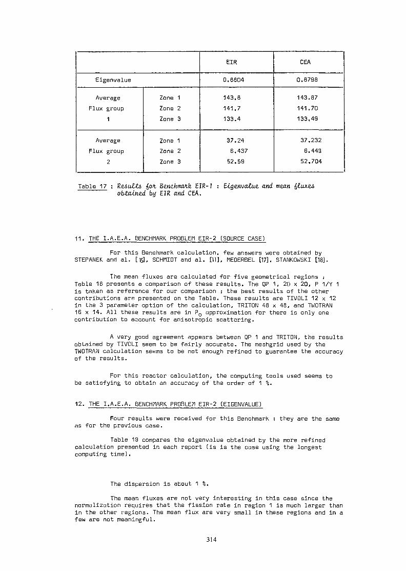
'Eigenvalue

AverageFlux group

1

AverageFlux group

2

Zone 1Zone 2Zone 3

Zone 1Zone 2Zone 3

EIR

0,8804

143.8141.7133.4

37.246,43752.59

CEA

0.8798

143.87141.70133,49

37.2326.44952.704

Table 17 ; Re/iu&ti faon. BencAmotfe EIR-7 : Ecgenvoûe and mzanobtained by EIR and CEA.

11. THE I.A.E.A. BENCHMARK PROBLEM EIR-2 (SOURCE CASE)

For this Benehmark calculation, few answers were obtained bySTEPANEK and al. [15], SCHMIDT and al. [11], MEDERBEL [17], STANKOWSKI [18].

The mean fluxes are calculated for five geometrical regions ;Table 18 presents a comparison of these results. The QP 1, 20 x 20, P 1/Y 1is taken as reference for our comparison ; the best results of the othercontributions are presented on the Table. These results are TIVOLI 12 x 12in the 3 parameter option of the calculation, TRITON 48 x 48, and TWOTRAN16 x 14. All these results are in PQ approximation for there is only onecontribution to account for anisotropic scattering.

A very good agreement appears between OP 1 and TRITON, the resultsobtained by TIVOLI seem to be fairly accurate. The meshgrid used by theTWOTRAN calculation seems to be not enough refined to guarantee the accuracyof the results.

For this reactor calculation, the computing tools used seems tobe satisfying to obtain an accuracy of the order of 1 %.

12. THE I.A.E.A. BENCHMARK PROBLEM EIR-2 [EIGENVALUE]

Four results were received for this Benchmarkas for the previous case.

they are the same

Table 19 compares the eigenvalue obtained by the more refinedcalculation presented in each report (is is the case using the longestcomputing time).

The dispersion is about 1 %,The mean fluxes are not very interesting in this case since the

normalization requires that the fission rate in region 1 is much larger thanin the other regions. The mean flux are very small in these regions and in afew are not meaningful.

314

Ré-gion

1

2

3

4

5

Ref.QP1 2 0 x 2 0

0.7921 10~2

0.3727 10~3

0.1268 10"1

0.5827 10~3

0.103010'1

TIVOLI12 x 12

0.78157 1C"2

0.39565 10~3

0.12415 10"1

0.62906 10~3

0.10512 10~2

Ref-TM)LJRef(%)

+ 1.3

- 6.2

+ 2.1

- 7.9

- 2.1

TRITON48 x 48

0.7896 10~2

0.3818 10~3

0.1266 10"1

0.585010"3

0.103310'2

Ref-TRTJONTRITONm

+ 0.32

- 2.4

+ 0.16

- 0.39

- 0.29

TWOTRAN16 x 14

0.7900 10~2

0.3127 10~3

0.1263 10"1

0.6853 10~3

0.9893 10~3

Ref^TWGTR/WRefm

+ 0.27

+ 16.1

+ 0.39

- 17.6

+ 3.9

Table 18 : CompMAAon on tiio. Mean F£uxei jjo/t Benchmark EIR-2 a.

QP 116 x 16 P1/Y1

1.0046

TIVOLI12 x 12 linear

0.99871

TRITON24 x 24

0,9983

TWOTRAN

1.0076

Table 19 : Compa/UAon o£ thé. exl Bzndimafik EIR-2 b.

CONCLUSION

The comparison of the accuracy of the results during the five yearsof the CRP shows the important development of the accuracy of the numericalmethods due to the research work performed by all the teams.

This Kind of international cooperation should be further encouragedin the future by either enlarging the field of applicability and the natureof the benchmark problem to be proposed and improving the exchange ofinformations between the different teams.

REFERENCES

[1] ENGLE W.W., Jr, "A One Dimensional Discrete Ordinate Transport Code withAnisotropie Scattering"K - 1693, Oak Ridge, Tennessee.

[2] J. STEPANEK, J. LIGOU "A Solution of the Coupled Integral and DifferentialForm of the Transport Equation Using a Legendre Polynomials Source DensityApproximation in Angle and Space for Slab Geometry"Proceedings of the Fourth International Conference on Reactor Shielding(Paris 9-13 oct. 1972) Part 2, p. 302,

[33 BOFFI V., MOLINARI V. "Heterogeneous Methods in Neutron Transport Theory"CNEN Report - RT/FI (68) 30 - Rome (1968).

[%] BOSEVSKI T., POP JORDANOV J. "Solution of Integral Transport Equation inSpace and Energy Points with Polynomial Interpolation"Numerical Reactor Calculations, I.A.E.A., Vienna (1972), 329.

315

[5] J. STEPANEK, J. LIGOU "EIR-BenchmarK Neutron Transport Problem Computation•For IAEA Coordinated Research Program"EIR [1974).

[6] A. KAVENOKY "The CN Method of Solving the Transport Equation. Applicationto Plane Geometry"Nucl. Sei. and Eng. 1978, 65, 2, p. 209.

[7] J. LIGOU "Improved Integral Transport Theory by Mean of Space PolynomialApproximations"Nucl. Sei. and Eng. 50 (1973) p. 135.

[8] POP JORDANOV J., BOSEVSKI T., KOCIC A., ALTIPARMAKOV D. "A Study ofCollision Probability and Monte Carlo Approaches to Integral TransportTheory for Heterogeneous Media"IAEA Specialist Meeting on Methods of Neutron Transport Theory in ReactorCalculations, Bologna, Italy 3-5 Nov. 1975.

[9] CARLVIK I. "Calculation of Neutron Flux Distributions by Means ofIntegral Transport Methods"AE-279 [1967).

[10] SANCHEZ R. "Results for the First and Second CEA Benchmarks"[11] M. MESINA, F.A.R. SCHMIDT, D. WOERNER "IKE Benchmark Compuations for the

IAEA Coordinated Research Program"

[12] E. CUPINI , A. DE MATTEIS, R. SIMONINI "KIM, un programma Monte Carlobidimensionale per reattori termici"CNEN Internai Report RI T/FIS-LMA [79).

[13] T. DURACZ "Results of the IAEA Benchmark Problems CEA 1 and CEA 2"Computing Center Cyfronet 1978.

[14] K. TCHUCHIHASHI "CLUP 77 : A Fortran Program of Collision Probabilitiesfor Square Clustered Assembly"JAERI 1196 [1971).

[15] C. HIGGS, C. MAEDER, J. STEPANEK "EIR - Benchmark Computations for IAEACoordinated Research Program,

[16] A. KAVENOKY, M. LAM HIME, Z. STANKOVSKI "Improvements of the IntegralTransport Theory Method"Computational Methods in Nuclear Engineering, April 23-25 1979, Williamsburgp. 7-55.

[17] Y. MEDERBEL "Results for the EIR-2 Benchmark Problem",

[18] Z. STANKQVSKI "Results for the EIR 2 Benchmark Problem".

316

A N N E X

the. Bencfwiotfe P/ioblm&

BENCHMARK PROBLEM SWIERK-1

Calculation of Keff

Geometry; mono-dimensional plane three-layer systemEnergy groups : one-energy groupScattering ; isotropic

Geometrical data

Layer n. 1 n. 2 n. 3Material n. 2 n. 1 n. 2Thickness 1.8 cm 4.95 cm 1.8 cm

Boundary conditions

BoundaryCondition

MaterialCapture+Fission

Scattering jLS

VX Fission vZ

Total 2. (cm1

Left:Vacuum

Nuclear Data

JET (cm )a(cm~1)(cm"1}

-1>

Right:Vacuum

n. 10.065

1.200

0.090

1.265

n. 20.0195

2.0405

0.000

2.0600


Calculation of neutron escape probability, P

P = Probability that a neutron produced by a distributed(P ) or localized (Pc ) source escapes from thea,c «•>body for the first time after any number od collisions;

317

P = probability that a neutron generated by fission escapescrfor the first time after any number of collisionsbefore it generates a new fission in a critical slab.

Geometry : monodimensional plane slab of optical half-thickness a = 0.0001; 0.005; 1,2,3.

Energy groups: one - energy group

Scattering; isotropic or linearly anisotropic(W = 1);W. = 3 f>~ =0.1; 0.2)o 1 ' o

Number of secondary neutrojis por scattering;

c = —~- = 0.001; 0.01; 0.2; 0.4; 0.6; 0.8; 0.9,s Z


Calculation of the flux ratio /£> in a cylindrical cellm T r

c|> = average thermal neutron flux in the moderator;1 mct> = average thermal neutron flux in the absorber rod.

Energy groups; one-energy group

Scattering in the moderator; isotropic ( u, =0) or linearlyanisotropic (^ = 0.2)

Source; uniform source of thermal neutrons in the moderator.

Geometry; infinite absorber rod of radius r =2cm. insidethe infinite annular moderator cylinder ofexternal radius r = 12 cm.

^gUclear data; absorber rod: 2. =10 cm

£ » 0; p.

moderator:

3 * °*

7a =0; .cl

T -1</ = 0.4 cm ; IJL- =06 1 O

and 0.2

318

BENCHMARK PROBLEM 5WIERK-4

Calculation of K of the Swedish fast zero power

reactor FR-0 (Report AE-279).

Energy groups; threeScattering; isotropicGeometry; sphere with fuel zone surrounded by a reflector

(radius r = 17 cm. and r = 47 cnu).

Nuclear dataEnergy group

Spectrum v

y x Fission vjîf (cm ) .

«y / — 1Total Z (cm ) .

Scattering En.

Group

g

1

2

3

0.57400-0

0.77910-1

0.19836-0

0,85520-1

0.

0.

0.38300-0

0.27660-1

0.28614-0

0.26091-0

0.77670-1

0,

0.33000-1

0.38150-1

0.50872-0

0.47814-0

0.76500-2

0,62300-2

1. IAEBA Benchmark Problem EIR 1 for x-y geometry

LWR Fuel Element with Burnable Poison CellGeometry

dimension Material Numbers1.5

1 . 6

1 - 6

1 . 6

1 . 6

1 . 0

Dimension

A3

3

3

3

3

3

1.5

1

1

1

1

3

1.6

2

1

1

3

1.6

1

1

3

1.6

1

3

1.63ß

1.0

Boundary conditions: Reflective on all four sidesSymmetry: Mirror symmetry with respect to the diagonal AB

319

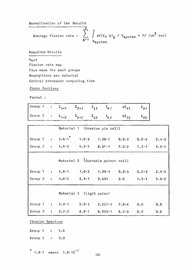
Normalisation of the Results

Average fission rate dV(Ef $)g / V&ystem = 1/ (cm sec)Vsystem

Required ResultskeffFission rate mapFlux maps for each groupsAbsorptions per materialCentral processor computing time

Cross Sections

Format :

Group 1 : £.

Group 2 : £

>1 E2-*1 Et1 rai vEf<| Sf1

*2 E2+2 Et2 Za2 v Ef2 Sf2

Group 1 :Group 2 :

Group 1 :Group 2 :

Group 1 :Group 2 :

Material

1.8-1*1.0-2

Material

1.8-11..0-2

Material

2.0-12.2-2

1 (Uranium pin

1.0-3 1.99-15.3-1 6.01-1

cell)

9.0-37.0-2

6.2-3 2.4-31.1-1 4.5-2

f.2 (Burnable poison cell)

1.0-3 1.99-15.3-1 3.531

3 (Light water)

2.0-3 2.227-8.8-1 8.900-

9.0-33.0

1 7.0-41 8.0-3

6.2-3 2.4-31.1-1 4.5-2

0.0 0.00.0 0.0

Fission Spectrum

Group 1Group 2

1.00.0

* -11.8-1 means 1.8-10 320

2. IAEA Benchmark problem EIR, 2 for x-y geometry

a. §2y.r.2§_P.roblemOne energy group anisotropic scattering, 5 materials, 5 zoneseach with material of the same numberSource : flat, isotropical

in zones 1 and 3, 0 s 1in zones 2, 4 and 5 0=0

Boundary condition : vacuum

x-y Geometry

18.0

25.0

25.0

18.0

4

1

3

25

18.0 30.0 30.0 18.0

Cross SectionsMater ia l

1

2

3

4

5

I.a

0.07

0.28

0.04

0.15

0.01

vlf

0.0

0.0

0.0

0.0

0.0

Et0.60

0.48

0.70

0.65

0.90

Eso

0.53

0.20

0.66

0. 50

0 .69

E .s1

0.27

0.02

0.30

0.15

0.40

E _s2

0.10

0.01

0.20

0. 10

0.10

The problem differs from the problem a. by source andproduction cross sections;in all zones Q = 0.

321

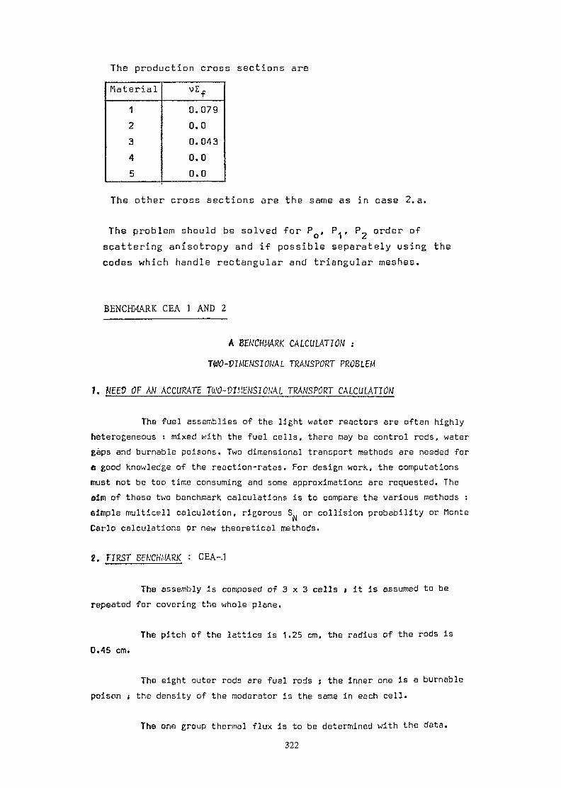
The product ion cross sections are

Material12345

vEf0.0790.00.0430.00.0

The other cross sections are the same as in case 2.a.

The problem should be solved -for P , P., P_ order ofscattering an î so t ropy and if possible separately us ing thecodes which handle rectangular and tr iangular meshes.

BENCHMARK CEA 1 AND 2

A BENCHMARK CALCULATION :

TWO-DIMENSIONAL TRANSPORT PROBLEM

1. KEEP OF AN ACCURATE Tù.'0-PIMENSIO.VAL TRANSPORT CALCULATION

The fuel assemblies of the light water reactors are often highlyheterogeneous : mixed with the fuel cells, there may be control rods, watergaps and burnable poisons. Two dimensional transport methods are nesded fora good Knowledge of the reaction-rates. For design worK, the computationsmust not be too time consuming and some approximations are requested. Theaim of these two benchmark calculations is to compare the various methods :simple multicsll calculation, rigorous S or collision probability or MonteCarlo calculations or new theoretical methods.

2. FIRST BENCHMARK : CEA-.1

The assembly is composed of 3 x 3 cells ; it is assumed to berepeated for covering the whole plane.

The pitch of the lattice is 1.25 cm. the radius of the rods is0.45 cm.

The eight outer rods are fuel rods j the inner one is a burnablepoison ; the density of the moderator is the same in each cell.

The one group thermal flux is to be determined with the data.322

QOOOo

Source density

Zt

la

Moderator

1.

1.25 < cm"1

8.10~3 cm"1

Fuel

0.

0.625 cm"1

0.270 cm"1

Burnable poison

0.

14. cm

14. cm

The mean flux and the absorption rate are to be determined forsix regions : results are to be presented an Table 1 of Annex 1.

S, SECOMV BENCHMARK ; CEA^Z

The assembly is composed of 7 x 7 cells of the same size as in theprevious case : there is one water gap in the center and eight poison cells.

Burnablepoison

Watergap

OOOOOOO

14

18

1610

The conditions are the same j the flux and reaction rates are tocalculated for the 19 numbered regions (Table 1 of the Annex 2).

323

Chapter VIII

OTHER APPLICATIONS

J. LIGOU, P. BENOIST, V. BOFFI, B. STENIC

The diffusion of neutrons in materials is governed, with a high degree

of accuracy, by the so-called neutron transport equation. This equation

plays therefore a very important role in reactor physics so that a

tremendous work has been devoted to the numerical analysis of such an

equation as shown in the previous chapters.

As a matter of fact the neutron transport equation is simply the linear

form of the Boltzmann equation in which the distribution functions of field

particles (for example atom nuclei in a fission reactor) are known. On

the other hand L. Boltzmann has derived his equation one century ago

in connection with the kinetic theory of gases. One can therefore stress

that such an equation can be applied to many transport phenomena. More-

over one has to keep in mind that very powerful methods have been

developed for reactor physics applications and some of them could be

used, at least as guidelines, to solve quite different problems. Such an

approach should be very fruitful.

To this end new applications of the transport theory have been inves-

tigated by four groups in Italy, France, Switzerland and Yugoslavia.

Several problems dealing with Controlled Thermonuclear Reactors have

been analyzed at Ecole Polytechnique Fédérale de Lausanne by P.A. HALDYand J. LIGOU with the help of M. CARO (Sect. 1). The Boltzmann equation

can also be used in the theory of Non-linear Electrical Conductivity as

shown by V. C. BOFFI and V. G. MOLINARI at Université di Bologna

(Sect. 2). In a very different field a special transport equation has been

applied to material sciences by P. BENOIST and G. MARTIN at Saclay

(Sect. 3). Other applications have been proposed at University of Belgrade

by Lj. ARSOV, J. POP-JORDANOV, R. SIMONIC and B.V. STANIC

(Sect. 4).

From the achieved results, the author is convinced that many else

applications could be found.

*Report written by J. LIGOU

325

1. APPLICATION OF TRANSPORT THEORY TOCONTROLLED THERMONUCLEAR REACTOR PROBLEMS

It is clear that neutronic calculations of fusion (or hybrid) reactor

blankets can be performed with standard neutron transport codes, at

least for steady state cases. Nevertheless some peculiar problems

related to neutron space kinetics will occur with pulsed reactors.

There are very few time dependent neutron transport codes and they

should be probably improved:

- The usual time discretisation leads to a pseudo-steady-state equation

in which very large neutron macroscopic cross-sections are built up

when small time steps are chosen and that can require a special

treatment. For charged particles the problem appears already in

the steady state case since the multigroup removal cross-sections

derived from the continuous-slowing-down scheme are very large for

narrow energy groups (Sect. 1-1-3). It is interesting to point out

that for time dependent problems all kinds of test particles (neutrons,

ions, etc. ) require similar technique.

- With the inertial confinement approach to fusion other kinetic problemsarise. For example during the expansion phase of a compressed pellet

one has to compute the energy deposition of fast particles (alphas,

neutrons) resulting from fusion events. The transport equation is now

coupled to hydrodynamic equations.. Because the equations of motion

are generally expressed in terms of Lagrangian coordinates, the same

choice should be made in the transport equation and doing that the

space meshes "will follow" the pellet expansion. Moreover in a fast

moving medium the angular flux must be defined as a function of

the relative velocity (with respect to the medium). With the new

variables the Boltzmann equation takes the usual form except a new/ _ Sf \term involving the velocity gradient of the flux ( A • —=• J. A similar

term is expected for charged particle transport equation with external

fields, but here its origin is quite different and it will appear even

for neutrons provided the considered medium is moving. (Sect. 1. 5)

One sees with these both examples that there is a strong connection

between some special neutron kinetic problems and charged particle

transport. When a good technique has been found to solve the correspond-

ing equations, two physically different problems have in fact been solved.

This will be made clearer in the next sections.

326

Coming back to time independent problems it is perhaps less obvious

that some of the existing methods used in neutron transport theory can

be applied to plasma physics. This requires of course, special modific-

ations of the formalism which are sometimes not trivial but roughly

speaking one has still to consider the usual three classes of methods:DSN, PN, Integral Transport.

In the absence of external fields the main difference between neutrons

and charged particles propagating in a plasma comes from the scattering

cross-section. Due to the long range of Coulomb forces this cross-

section is very anisotropic for charged particle interactions with plasmas

and the usual scattering integral operator must be abandoned for practical

reasons although it remains valid in principle. The so-called Fokker-

Planck operator which incorporates the peculiarities of charged particles

interactions seems much simpler at first glance because it has a different-

ial form. But «in practice it brings new difficulties which were not met

with neutrons (their scattering cross-sections are rather Isotropie up

to 50 keV). In fact for high energetic neutrons the cross-sections are

also very anisotropic so that the difficulties should be the same and it is

known that many Legendre scattering matrices are needed in this case.

Here also a feedback becomes evident: a suitable technics for charged

particle could be at least partially applied to fast neutron problems. (Sect. 1.4)

Another difference which is again related to the long range of Coulomb

forces may come from collective effects. In other words the test

particles can interact with the plasma as a whole. This is a collision-

less mechanism which is a typical problem in plasma physics (Sect. 1. 2).

Here the formalism is rather far from those met in neutron transport

theory, but nevertheless some tricks of the PN theory can be used.

In short a first list of problems which are both important for

Controlled Thermonuclear Reactor (CTR) and tractable by using modified

neutron transport methods can be settled down as follows:

1. Fast Ion Transport in Plasmas: Energy deposition or ignition of

compressed DT pellets by alpha heating, ion beam fusion, etc.

2. Turbulent Electron Beam - Plasma Interaction: General interest in

plasma physics.

3. Point neutron kinetics for fissionable pellets: This is a classical

reactor kinetic problem except that the neutron source used for

ignition should be weighted correctly.

327

4. Fast Ion Transport in Solids: It has been proposed to use neutron

transport codes, but one can show that the methods developed for

plasmas (1st point) can bring new ideas: erosion of the first wall

in a CTR (Sputtering)

5. Time dependent transport equation in a moving medium described

by hydrodynamic equations (Lagrangian coordinates): energy

deposition of alphas, neutrons, etc. in an expanding pellet.

Most of our research work has been devoted to the first three points,

but preliminary theoretical results have been obtained concerning the

last two. It came out from these studies that the connections with the

fission reactor physics were deeper than it was thought before so that

the above list could be probably stretched out.

1.1 Fas t Ion T r a n s p o r t in P l a s m a s

The interaction of energetic ions with plasmas is a very important

problem in controlled thermonuclear fusion. For example, this ion

population may represent either the a-particles resulting from D-Treactions or an external beam used for plasma heating or pellet

compression (SHEARER, 1975). If we restrict the analysis to collisional

phenomena, the plasma may be defined as a given gas (ions + electrons)

which is in thermal equilibrium, and, then, the fast-ion distribution

function is ruled by a linear kinetic equation. Basically, this equation

has the same form as the neutron or photon transport equations and

therefore some of the techniques used in reactor physics can be applied.

We have, of course, to take into account the pecularities of Coulomb

scattering which can lead to highly anisotropic fluxes.

So far, only very crude approaches or time-consuming Monte-Carlo

calculations have been used. More recently a modified multigroup

diffusion scheme (CCRMAN et al, 1975) has been proposed to solve this

problem, but this method is not accurate enough when the flux anisotropy

is too important (ion beam, localized sources, etc. ). It is therefore

necessary to start with the initial transport equation itself:

g ( xs ^ a \ mv

r m-^- —- G (x ) ^- (1-H.2) f*- \ + S ( r , v , n , t ) (D2 v m a ôg. 9).

328

The right-hand side of this equation results from the Fokker-Planck

approximation which states that only small energy transfers and small

scattering angles occur during collisions. Moreover, it is assumed that

the direction of the particles is defined by only one variable, |_i, the

deflection cosine. This means, in practice, that only one-dimensional

geometries (plane or spherical) are considered (COŒEÎR, 1970).

The distribution function $ ( r , v, ( j , t ) and the sources S ( r, v, u , t ) are

defined in the usual sense and the subscript "a" refers to either plasma

ions or electrons. The coefficients of the Fokker-Planck operator are

defined as follows:

4 r r NF =a m m In A

2"

-

~

(2)

"X

2 =m v2

a

26

m

me

where z , m , N , 8 , In A are respectively the atomic number,a a a a athe mass, the particle density, the temperature and the Coulomb

logarithm of the plasma component "a", z, m refer, in the same way,to the fast-ion population.

For the present application, it is more convenient to choose the

energy E = (l/2)mv2 as basic variable and, moreover, to introducethe fluxes cp. Then, for plane geometry, the Fokker-Planck equation

takes the form (with $ = (m/v 2 ) cp ) :

g

329

with C = •£a 2

m

If we only consider the slowing-down domain (E > 9 ), the termsg a

9 /E and 9 —— can be eliminated from Eq. (3).a a oil

Moreover in most cases (hot plasmas) the functions g(x ) andaG(x ) can be simplified considerably. For plasma ions the condition

a mi /E \E » 9. leads to x? = —— (— ) » 1 since m- and m are of the samei i m \ 0J / iorder of magnitude. On the contrary, x for the electrons is very

small if E « —— Q . This condition is fulfilled in a large domain,m e &e

We can therefore write:

g(x.) ~ G (x.)

Then for steady state problems we obtain the final form of the ion

transport equation for hot plasmas with electron density N :

Sec ,T r aI-1 N ÊTâx e L SE (4)

where

U(E) = — + a /Ê" (microscopic stopping power)

T(E) =

(5)

The interactions with electrons are represented by the term a /E

and the collisions with ions by b/E and c/E2.

For compound plasmas with several ion species the coefficients a,

b, c are defined by the following relationships:

b =

c =

m

z * l n A . (6)

* In A.

330

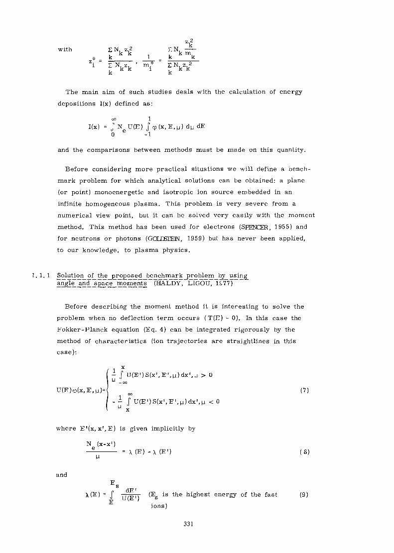
z|with EN, z,2 EN, ——, k k , . k m,# _ k____ l _ k____k

Zi E N. z. ' ïnT " E N . z. 2, k k i k kk k

The main aim of such studies deals with the calculation of energy

depositions I(x) defined as:

00 1

I(x) = J" N U(E) J cp(x, E , M ) d|_i dEo e - i

and the comparisons between methods must be made on this quantity.

Before considering more practical situations we will define a bench-

mark problem for which analytical solutions can be obtained: a plane

(or point) monoenergetic and isotropic ion source embedded in an

infinite homogeneous plasma. This problem is very severe from a

numerical view point, but it can be solved very easily with the moment

method. This method has been used for electrons (SPENCER, 1955) and

for neutrons or photons (GOLD3TE1N, 1959) but has never been applied,

to our knowledge, to plasma physics.

1. 1. 1 ^2_l^tioj^£f_tJ^_pj^£<^j3d__bj3nângle and space moments (HALDY, LIGOU, 1S77)

Before describing the moment method it is interesting to solve the

problem when no deflection term occurs (T(E) = 0). In this case the

Fokker-Planck equation (Eq. 4) can be integrated rigorously by the

method of characteristics (ion trajectories are straightlines in thiscase):

U(E)cp(x,E,Li)=

x- J U(E ' )S(x ' ,E ' ,u )dx ' , M > 0

1 1 ', <0

(7)

x

where E'(x, x' .E) is given implicitly by

N (x-x1)—————— = X (E) - X (EM (8)

and

j-rp j

X ( E ) = J u (EM Ês is the hiSnest energy of tne fast (9)ions )

331

The correlation between (x,E) and (x'.E1) for each direction is a

typical feature of the continuous-slowing-down model. This property

is smeared out when approximations are made on the angular fluxes,

for example in the diffusion theory.

gFor a plane monoenergetic Isotropie source S(x,E, ja) =— 6(x) 6(Eo-E)

the scalar flux exhibits a flat space distribution:

N SN U(E) cp (x, E) = __ for | N x | < x (g)

Finally the expression for the energy deposition I (x) is readily

derived:

E*(x) N S E*(x)I p l ( x ) = J N e U(E)cp 0 (x ,E)dE -~~l ^

with x(E*) = Nx = J1 L (see Eq. (9) )

The corresponding I (x) for point monoenergetic sources can beobtained using the trick:

d l ( x )

or with Eq. 11:

4rrx2 I (x) = S Ng U[E* (x) ] (13)

This last expression defines a curve which exhibits the expected

Bragg profile. The equation (9) shows that the maximum range is

reached when E*= 0, this means that x. = TTT— .e

In most hydrodynamic codes used for inertial confinement studiesthe transport of charged particles is more or less based on the above

formalism although some supplementary approximations are often

introduced. The remaining question is whai are we allowed to neglect

the ion scattering process ? The moment method will answer this

question. Coming back to the Eq. 4 (with T(E ) •£ 0) one first derives

the P equations (for a plane isotropic .and monoenergetic source at

x = 0)

6 (x)

332

then introducing the space moments

N x n(14)

with the convention Y =0 when n < 0 one obtains a closed setn, eof equations:

n-1

n, • 2e+i 2e+i X 6 ( X )

(15)

where the more convenient variable X has been introduced instead of

E (Eq. 9). After integration over \ the explicit expression for Y

comes out:

1 n n, ;c e(x X1 1-1 (16)

with: C (X) = exp - g ( e + l ) J T ( x ' ) dx'o

By using the simplest form of U(E) and T(E) (Eq. 5) one gets the

analytical expressions:

2/3 [ê

(17)

1+aE 3/2

(18a)

1/3 1/3 1/3

(18b)

... . . 1 , 1with 9(x) = In 1 , -1 2x - 1tan

When the moments are known for (n-1) the Ea. 15 provides R (\)Tiy c

and then Eq. 16 is integrated numerically. This can be done easily

because the Y have been defined in such a way (Eq. 14) that they•**j Y/ »

are very regular functions of \. When c =0 (no deflection) C =1

the previous equations show that:

Y (\) = 1 and this was expected from Eq. 10,14.

333

One can easily see that the Y cancel when ? > n and (n + e) is odd.

This is a peculiarity of isotropic sources. One has therefore to evaluate

the set:

Y0.0 = l' Y 1,1 ( X ) ' Y 2,0 U ) ' \2 ( X ) ' Y 3,1 U ) < etc'

We have now to construct ep (x,E) from the space moments.

One starts from a physical argument. All fast ions with the energy EX (E ) X (E )remain in the interval - —-;—- < K < -r^—- as it has been proved wheni\ JN

T (E) = 0 (see Eq. 10). This statement is still correct when deflections

occur and is a consequence of the continuous slowing-down model. It

seems therefore reasonable to expand cp over space Legendre polynomial/ \ (E) ° \(E) \series over the finite interval ( - -^—- , + -^—- j :* J.N o J.\ _ /

S Z ^ - l ^ <19)

m=o

with the inverse transform:

X/Ne N U(E)cp (x,E) N xf ( E ) = ; -2 —— ——— P (-^-m - x / N S mV X

' e

Using the expression of Legendre polynomials:

mp m ( S ) . z Çf'

p=o

one can obtain the Legendre coefficients f (E) as a function of the

moments Y :n, o

m Y (E)

'E ' S •" Tî-p=o

An integration of the Eq. 19 over energy will finally provide the

energy deposition;

I (x) - J N U(E)cp (x,E)dE =S S ^_ J % em=o

N |x|f (E)P ( e._. dEm m V X (E )

N |xwith X(E*) = N x and

334

X ( E ) can be seen as a table resulting from Eq. 18b and the values of

x may be chosen in such a way that no interpolation has to be made

in this table. The maximum range x is then defined as \ (o) /N .

As said before, when no deflection occurs, all the Y are unity.

It follows that all Legendre coefficients f cancel except the first one

fQ= 1. The Eq. 19 and 21 become identical to the Eq. 10 and 11.

The first term in the series (19-21) can be seen as the "Bragg"

part of the solution. The higher modes result from the ion deflection

(scattering without energy loss).

The energy deposition distribution for a point source is always

given by Eq. 12, a numerical derivation of Eq. 21 is therefore needed.

If one is interested by the deposition to electrons or plasma ions theUe Ui

ratios—- (E) or — (E) must be introduced in the Eq. 19-21.

The proposed benchmark problem is therefore completely solved.

A Fortran program named ODYSSEY has been developed and many

calculations were performed from which some conclusion can be drawn

(HALEST, 1977):

For the transport of alpha ions in D-T plasmas the scattering is not

very important and the diffusion theory (CQRMÄN, 1975) can be in error.

In this case it is probably better to neglect the deflection term in the

Fokker-Planck equation and then exact solutions can be found (Eq. 13).

In other words the "Bragg" profile gives a reasonable energy distribution.

On the other hand for heavier plasma ions and (or) lighter energeticmiions (—— > 2) the collisions without energy loss are more and more

important, mainly •when the slowing-down due to plasma electronsmidecreases. For intermediate values of the ratio — , roughly speaking

between 1 and 8, one cannot avoid to solve correctly the Fokker-Planck

equation with the scattering terms, at least for localized source problems.

Beyond, the diffusion theory becomes probably valid.

As an example, the Fig. 8.1 displays the results concerning a 1 MeV

proton Isotropie source in a B D1 T.. plasma at solid density1.0 -L. D

(Ne = 2. 5 1022 cm-3, ~z[ = 3. 5, m'i= 1. 95, 6 = 50 keV, m = Z = 1).

For this composition the maximum proton range is x = = 1.06 cm.

For deep penetrations the energy deposition of 1 MeV protons to

plasma ions exceeds the deposition to electrons. At such distance from

the source the protons are rather slow so that the electron contribution

to the stopping power given by Eq. 5 becomes small.335

In the Eq. 21 the series must be somehow truncated. Most calculations

have been performed with 6 LP coefficients (m< 10). To check the

convergence of the series a few calculations have been made with 11 LP

coefficients (m <, 20). As shown by the Fig. &1 the discrepancies are not

very pronounced. The lack of harmonics appears mainly at large distances

from the source where the 6 LP approximation exhibits a small "swing"

v,ith negative values. These numerical oscillations are acceptable in

practice and their size gives an idea of the accuracy of I ho results.

They disappear with the 11 LP approximation. Finally üio Bragg curve

!1 LP approximation) has been reproduced on i . r>e Fig.8.1. The comparison

w i t h the exact solution shows the importance of the scattering process.

The moment method can be applied to anisotropic plane sources:

s (x, E , U ) ':: s • £p- (-^=- ;• 5 (x) * (i

(p •• 0 corresponds to isotropic sources)

The whole formalism remains the same, but manv more Yn, ?

have 10 be computed (n-.-z is not necessarily even).

In the Fq. 15 for example *, is replaced by S. wi th :

,, P+1-? ,.. , -, ,b •• *-—-.—— ü , and b - 1?. p+1+2 K-1 o

and this new benchmark problem simulates the in terac t ion of ion

beams, more or less collimalod (depending on p value) , wi th plasmas (ÏTA.LOY, 1979).

1 . 1 . 2 CJr(H.>n_runcti()ns (T.CXX;, Il-MDY, 1978)

As it has been said the previous theory can be used to check the

accuracy of numerical methods v,hich have to be developed for more

practical cases (inhomogeneous plasmas). Nevertheless the above

results can be used directly for any kind of voiumic source distributions

provided that the 'plasma can be considered as homogeneous. For that

it is interesting to define Green functions depending only on two para-

meters. Then the energy deposition profiles needed by hydrodynamics

codes are directly obtained from these universal functions. It is

convenient to use dimensionless variables:

EEnergy: -. = — (Es Energy of ion source)

Space: Ç = —— (x ._ Max. range of fast ions)XM

336

and "reduced" physical parameters (Eq. 6) :

a = m. /4m = c/b. /m~ m. In A E 3/2 aE 3 /24/e i e / js \ s

eP = 7T3 V Trm m z.

The Eq. 4-5 are rewritten in the form:

(22)

6 ( 5 ) 6 ( 1 - ^ ) (23)

U(r, ;ß) =

]X di;ß) = J"

il

dri1

("reduced" stopping power)

(fast ion range parameter)

where the plane source is assumed to be isotropic and monoenergetic

( 1 = 0 , n = 1).

The real maximum range is given by:

E 2

M (24)

By a similar procedure as before one obtains the energy deposition

in the following way:

E

Vs0 = GP i ( ? ; a 'ß )

1 Es 1~= 'J

Pt(x) = "

with the 'universal" Green functions:

(plane geometry)

2 + ( ? ; a , ß )pt

(point source)

G n l ( C : a , ß ) = X ( 0 . ß) J*o

pl

Gp t(§;a,ß) = - 2?^

with r|M(§) defined by:

§ = \ ( * 1 M ; ß ) / X ( 0 ; ß )

(25a)

(25b)

337

The scalar fluxes cp are computed as before with more convenient

space moments. The code ODYSSEY has been extended to the comput-

ation of Green functions. Starting from the physical data: 9 , m. , z. ,6 1 1

etc. the basic parameters a, ß are calculated and then Eq. 23 is

solved. One can also choose a, ß as input parameters. For given

a, ß values one Green function is produced, but it represents in fact

several physical situations.

Even with too small a number of harmonics the approximated

distribution preserves the energy conservation:XM 1

Eg = J 4rr x2 I t (x) dx or J G t(§ ) df = 1 (see Eq. 25a)o P o P

On the source there is no ion scattering influence so that

G , (0 ; c t , ß ) = G (0;0, ß) = ( l + ß ) x ( 0 , ß ) (see Eq. 28,23 wherepi pinM(o) = D.

The influence of ion scattering is displayed on the Fig.8.2(ß = 3,

a = 0. 1 - 10). For alpha particles slowing down in a DT plasma,

a is small (a ^ 0.15), with protons in a boron hybride plasma (seeexample of section 1.1.1) «, reaches 2. Finally for ion beam fusiona high z external shell appears in many designs and a can be very

large (10 to 30). In these last two cases one sees that the ion deflection

cannot be neglected. The straightline trajectory assumption will provide

the right maximum range (Eq. 24) but a wrong profile (Fig.8.2).

The above Green functions can be introduced in hydrodynamic

calculations in the same way as it is done when the straight line

trajectory assumption is made (MO3ES, 1977) (LJQOU, 1978).

In a ID code the spherical plasma is divided into concentric zones.

Assuming as Moses did that fusion reaction products originate at the

center of the zone I, one can calculate, for example, the energy

deposition W in the zone III :Z

W = fff I . (x) x2dxJ J JZ TTTzone III

where x is the distance from the source taken on the direction 0

338

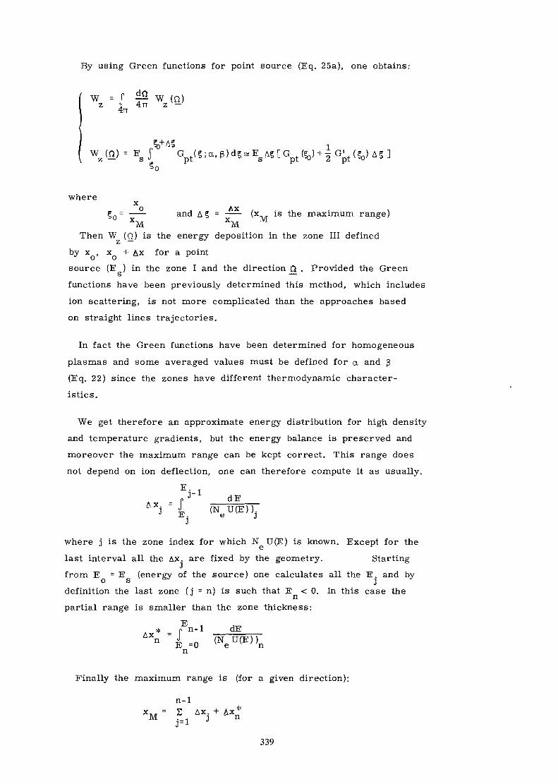
By using Green functions for point source (Eq. 25a), one obtains:

w = J w (n)z J 4rr z —4rr

(n) = E T- sJc

where

§0= —— and A? = —— (x is the maximum range)XM XM

Then W (Q) is the energy deposition in the zone III definedZ

by x , x + Ax for a point

source (E ) in the zone I and the direction Q . Provided the Greeng ——-

functions have been previously determined this method, which includes

ion scattering, is not more complicated than the approaches based

on straight lines trajectories.

In fact the Green functions have been determined for homogeneous

plasmas and some averaged values must be defined for a and ß

(Eq. 22) since the zones have different thermodynamic character-

istics.

We get therefore an approximate energy distribution for high density

and temperature gradients, but the energy balance is preserved and

moreover the maximum range can be kept correct. This range does

not depend on ion deflection, one can therefore compute it as usually.

P J " 1 dEJ " i_ (N e U(E)) .

J

where j is the zone index for which N U(E) is known. Except for the

last interval all the Ax. are fixed by the geometry. StartingJ

from E = E (energy of the source) one calculates all the E. and byo s jdefinition the last zone (j = n) is such that E < 0. In this case the

partial range is smaller than the zone thickness:

A < = l = on

Finally the maximum range is (for a given direction):

n-1XM = f=1

AXJ + AXn

339

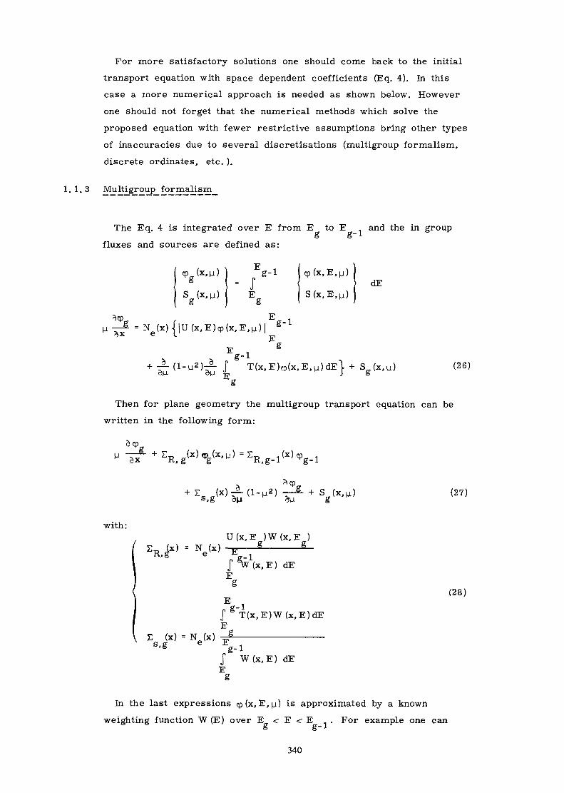
For more satisfactory solutions one should come back to the initial

transport equation with space dependent coefficients (Eq. 4). In this

case a more numerical approach is needed as shown below. However

one should not forget that the numerical methods which solve the

proposed equation with fewer restrictive assumptions bring other types

of inaccuracies due to several discretisations (multigroup formalism,

discrete ordinates, etc. ).

1.1.3

The Eq. 4 is integrated over E from E to E . and the in groupO 0

fluxes and sources are defined as:

cp„(x, n)g

Sg (x, n)

•pg-1= ;

Eg

Eg-1

Eg-1

cp (x, E,|j)

S(x,E.u)dE

T(x,E)cp(x,E,u)dE}. + Sg(x.n) (26)

Then for plane geometry the multigroup transport equation can be

written in the following form:

, g (x) = ER,g-i (x)

(27)

with:

x) = Ne(x)U(x,E )W (x, E )

g g

J ^W(x.E) dEE

E _g~

(x) = N (x)

T(x ,E)W(x ,E)dE

W(x ,E) dE

(28)

In the last expressions cp (x, E, |j) is approximated by a known

weighting function W (E) over E < E < E . For example one can

340

assume in each zone that the equilibrium spectrum is achieved. In

this case W(x, E) is the flux for an infinite homogeneous medium and

therefore W (x, E) ~ 1 v (Eq. 4 where ^ = 0, ^ = 0, S = 0).U(X, il ; o X an

Then the Eq. 28 takes a very simple form:

with

= Ne(x) / A x ( x )

(x) = Ng(x) J T ( x , x ) d X / A X g ( x )

g

(28 bis)

(x) = X(x, E ) - X (x, E J where X (E) is defined by the Eq. 9.s g- -iFinally if U and T take the form given by Eq. 5-6

N (x)

A X ( x )2 c3 b

1 +aE

(29)1 +

aE 3/2

where a, b, c depend on x (Eq. 6).

For narrow groups (AE -» 0) the removal cross-sections becomeD

very large and such a peculiarity did not occur in neutron transport

theory. The energy deposition I (x) can be calculated as follows:

GI (x) = E A (x) f (x) where § is the scalar flux derived from

g= !

the transport equation (Eq. 27) and

Vx ) =Vg ( x ) ( Eg-rV

At first glance one may think that standard SN codes can be used

to solve Eq. 27. This is in practice very difficult. For example with

the ANISN code the right hand side of Eq. 27 has to be expanded

into Legendre Polynomial series:

R.H.S. -

where the scattering matrices are defined as:

, g-l-»g HR, g-1

Js, g

341

and wC T(x) = J «Pa.(x»l-0 p» (u) d(aS _ l S "

For a localized source it has been impossible to produce meaningful

results with ANISN. This can be explained as follows:

It is not consistent to make a truncated expansion of cp * and to keep(e)the exact «p in Eq. 27. For neutron this is valid because the £

o

are decreasing when 8 increases but not here because of the strongly

anisotropy of the Coulomb scattering kernel. Therefore one has to

come back to Eq. 27. Moreover one can notice that any absorption

process of ions (nuclear reaction) can be incorporated easily in the

LHS of Eq. 27:

ER, g •* ZR, g + Ea, g Where 2a, g iS weiShted as

£S;g m Eq- 28.

The Eq. 27 is solved by the method of characteristics. For

U = |j (k = I, 2, ... N) one has to solve:K

uk —|- ( x >M k ) + £R ( X ) < P ( x >U k ) = q (x^k) (30a)

The scattering term D cp has been discretized as follows:

(30b)

.nk+i/2) - (i-u|_1/2)<^g (x.^k.1/2)w

K

where the W are the usual weighting factors for any quadrature1

scheme ( f CD du = S W. cp (u, ) ). If one chooses u i / 0 = - 1 and\J, jj k^ k / ^J-/^N

^N 1/9 = +^ tnen S W |D cp =0, in other words the identity

1t D cpd[j = 0 is fulfilled rigorously by our numerical scheme.

The derivatives cp(|_u ] ,„) can be approximated by

————— , but more accurate approximations can be found.

342

This procedure should avoid the difficulties met with ANISN since" pD cp is no longer replaced by -£ — — • e ( 6 + l ) c p P (p), moreover the

H 8=0 E

Eq. 30a is integrated analytically in each mesh (£ can be very largea g

so that — * cannot be approximated by a finite difference). For a giveno xmesh (x. n, x.) one obtains for the direction u :

1~ J. l K

Ti

1

forK.

with a similar equation when (j, > 0.

In the above equation one has set:

G(x) = l- 1^!

1 "x

H(x) = -e"X+ — — and TI = ^ |x.

where Z. represents the removal cross-section E for the mesh i.1 JTC,g

Starting from the right (i = J) with a given incoming flux cp(x ,(j )J K

one obtains all the c p ( x . , j i ) for |j < 0. For \± > 0 the system will1 K. K. K.

be swept from the left ( i = l ) to the right. When E ^0 one has

to iterate on q (x.,|_u ) which involves the unknown flux cp (Eq. 30b),

this is the usual inner iteration scheme.

Based on the above formalism a code has been completed veryrecently. The first checks will deal with the benchmark problem

described in previous sections for which very accurate results areavailable. When S =0 and £_ does not depend on x (homogeneous

s»g R>eplasma) the multigroup equations (Eq. 30) can be solved analytically

for a point source and a given direction (for example g. = 1 with afixed incoming current at x = 0 and Sg= 0). In this case we know the exact soJutbn

(sect. 1.1.1, Eq. 13). From this comparison it appeared that 20 energy

groups will give good results although this benchmark problem is very

severe (cp(x, E,|j = 1) is a singular function of E). This conclusion

should remain valid in most general cases and we will check that in

the near future.

The above multigroup scheme will be incorporated in the hydro-

dynamic code we intend to develop for pellet calculations (inertial

343

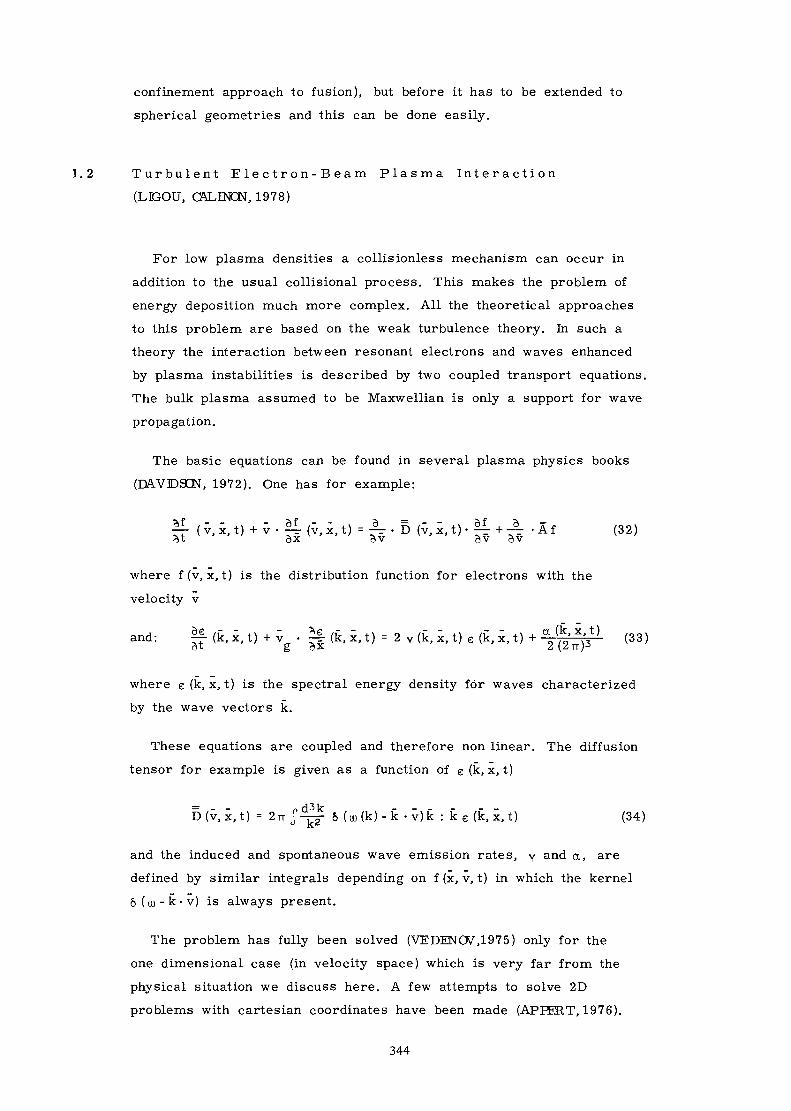
confinement approach to fusion), but before it has to be extended to

spherical geometries and this can be done easily.

1.2 T u r b u l e n t E le c t r on - B e am P l a s m a I n t e r a c t i o n

(LK3OU, CALINCN, 1978)

For low plasma densities a collisionless mechanism can occur in

addition to the usual collisional process. This makes the problem of

energy deposition much more complex. All the theoretical approaches

to this problem are based on the weak turbulence theory. In such a

theory the interaction between resonant electrons and waves enhanced

by plasma instabilities is described by two coupled transport equations.The bulk plasma assumed to be Maxwellian is only a support for wave

propagation.

The basic equations can be found in several plasma physics books

(DAVD9CN, 1972). One has for example:

(32)

where f (v, x, t) is the distribution function for electrons with the

velocity v

and: || (k. x. t) + v • *| (k. x. t) = 2 v (k. x. t) e (k. x, t) + ^ (33)

where e (k, x, t) is the spectral energy density for waves characterized

by the wave vectors k.

These equations are coupled and therefore non linear. The diffusion

tensor for example is given as a function of e (k, x, t)

D(v ,x , t ) = 2rr J ——^ 5 ( u u ( k ) - k - v ) k : k e (k, x, t) (34)

and the induced and spontaneous wave emission rates, y and a, are

defined by similar integrals depending on f (x, v, t) in which the kernel

o ( u ) - k - v ) is always present.

The problem has fully been solved (VEDENOV.1975) only for the

one dimensional case (in velocity space) which is very far from the

physical situation we discuss here. A few attempts to solve 2D

problems with cartesian coordinates have been made (APEERT, 1976).

344

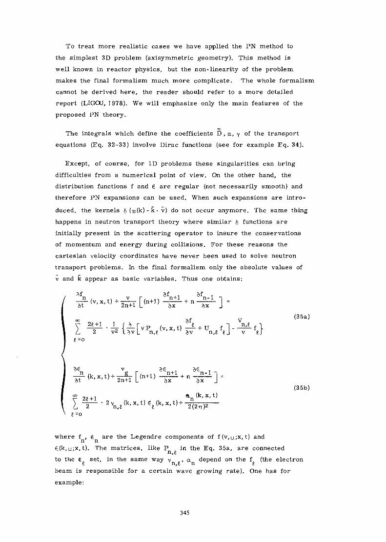
To treat more realistic cases we have applied the PN method to

the simplest 3D problem (axisymmetric geometry). This method is

well known in reactor physics, but the non-linearity of the problem

makes the final formalism much more complicate. The whole formalism

cannot be derived here, the reader should refer to a more detailed

report (LIGOU, 1978). We will emphasize only the main features of the

proposed PN theory.

The integrals which define the coefficients D , a, y °f the transportequations (Eq. 32-33) involve Dirac functions (see for example Eq. 34).

Except, of course, for ID problems these singularities can bring

difficulties from a numerical point of view. On the other hand, the

distribution functions f and € are regular (not necessarily smooth) and

therefore PN expansions can be used. When such expansions are intro-

duced, the kernels 6 ( i j u ( k ) - k - v) do not occur anymore. The same thing

happens in neutron transport theory where similar & functions are

initially present in the scattering operator to insure the conservations

of momentum and energy during collisions. For these reasons the

cartesian velocity coordinates have never been used to solve neutron

transport problems. In the final formalism only the absolute values of

v and k appear as basic variables. Thus one obtains:

^-(v.*,t) F /n4-1 ^ HT! U- 1 "1 _I IIJLT J. I i II ~L ôx 3x Jat "•-"' 2n+l

,, ,, (35a)oc gf v

Y ^r-^ ' 4r { — Fvp ( v , x , t ) — — + U f l - - ^ - f \L 2 v2 \3v L n , e v ' 3v n,« ej v eje = o

(35b)

e=o

where f , €, are the Legendre components of f (v, p.;x, t) and

€(k, |j;x, t). The matrices, like P in the Eq. 35a, are connectedn,6to the € set, in the same way v , a depend on the f (the electrono n^c n tbeam is responsible for a certain wave growing rate). One has for

example:

345

9 c; +1

— — — A D l ( v ) (36)s=o

,37)k(v)

where P is a Legendre Polynomial and w the plasma frequency:s 3u) (k) = 1 + - k2 (dispersion law).

From the properties of the coefficients A = T P P P dun, s,e J n s e M

a recursive formula can be derived:

(38)

P0( e (v) = D; (v)

Similar procedures can be applied to other matrices y » Q » ~+~n,6 n,e etc.

One can make the following remarks. Only single integrations have

to be performed numerically and no singularity appears in theintegrands (Eq. 37). Moreover all these integrals are evaluated

simultaneously for the whole set of v. . Then the recursive relation-

ships provide the required matrices (Eq. 38 for example). By this

way the computation time is reduced by a factor 10 as compared to

the time needed by the explicit form (Eq. 36).

In the transport equations (Eq. 35) the Legendre series must be

truncated somehow. In the program TURB we take e, n <, L for waves

and 6, n s L for particles. In practice L <r L because a realisticp ^ p wbeam can be represented with few harmonics.

The matrices are no more diagonal as in the collisional case

(harmonics coupling), one can therefore say that the space dependent

steady state equation (5/St = 0) is not more complicated than the time

dependent homogeneous equation (3/ox = 0). This is not true, of course,

with cartesian coordinates.

The second order differential operator in Eq. 35a is approximated

by finite differences. Then for homogeneous plasmas (-— = 0) one canoxwrite:

|f (i,t) = B (i , t )f ( i+ l , t ) -C ( i , t ) f (i.t) + D( i , t ) f (i-l,t) (39)ot

where i is the velocity mesh index and f = (f >.C

346

With a time centered discretization the Eq. 39 allows the calculation

of f (i, t ) from f (i, t 1 ) and all the coefficients are computed forAil * 4. ^jll~" -L

the time t_ at which the wave density 6 (i, t) is known. A full implicit^nscheme has of course to be applied to Eq. 39 and because of that we

have extended the well-known backward substitution method (Richtmeyer,

1967) to the vectorial form of a parabolic equation (Eq. 39).

A typical time of computation is 15 sec/timestep on a CDC 6500 for

70 velocity meshes and 10 Legendre polynomials (the parabolic equation

requires half of this time). This is quite reasonable for a non-linear

3D problem. The inhomogeneous problem (—— 0 but -—= 0), whichOX ot

is more realistic, should not take more time on each mesh Ax.

Unfortunately in many cases we could not reproduce the whole

phenomenon. After the waves have reached their maximum values the

program TURB gave wrong results. Up to now we could not explain

why this sort of numerical instabilities has occured with a full implicit

scheme.

1 . 3 P o i n t N e u t r o n K i n e t i c s

To ignite a fission chain reaction in a compressed plutonium pellet it

has been proposed to use fusion neutrons (LIGŒJ, 1977). This can be

achieved with a small central sphere of D-T materials. Then, one has

to solve in the simplest case the usual point kinetic equation with a

neutron source.

In such studies (microexplosions) one can forget the delayed neutrons.

All the kinetic parameters can be derived from steady state transport

calculation if the adiabatic approximation is made. The kinetic eigenvalue

a = -k- can be produced directly by standard transport codes. One can

show that the importance factor of the source K takes the form:

S >

where quantum mechanics notation have been used. In reactor physics

applications it has been assumed many times that K is unity. This is

only true when the neutron fission source and the extraneous source

have the same distribution (energy and space: S~ H $). For neutrons

347

resulting from spontaneous fission this is a good approximation, but

not for fusion neutrons which are more energetic (14 MeV). This

becomes even worse for localized sources. One should therefore compute

the adjoint fluxes $+. In fact this supplementary calculation can be

completely avoided if all unconverged eigenvalues are saved during a

standard transport calculation. The result is very simple (LIGOU, 1978):

• - -r ]

where k is the k value for the or outer iteration and k («. -» °°) the

converged eigenvalue. One sees that no extrawork is needed provided

the initial source used in the outer iteration scheme is the given source

and not an arbitrary distribution, as is generally made for a k search.

This important kinetic theorem allows straightforward calculations of

the importance factor and a better accuracy is achieved.

1 .4 F a s t Ion T r a n s p o r t in S o l i d s

In principle the Fokker -Planck formalism which has been applied

to plasmas (§ 1.1) could be kept here. In some cases however the large

scattering angle collisions should be introduced in the formalism if

the small backward ion fluxes have to be determined (sputtering yield

computation). In principle a pure integral operator over energy and

directions involve all kinds of collisions, but it will lead to a very

large number of Legendre scattering kernels (differential cross -sections

are very anisotropic for charged particles).

It has been proposed (HOFFMAN,1978) to keep the integral operator

only for large energy transfers (LET) and to add the usual continuous

slowing down operator (CSD) for small energy transfers (SET). This

is not quite consistent. We could show recently (LIGOU, 1979), starting

from the integral operator, that the SET part should be represented

by a complete Fokker-Planck operator (see Eq. 4) and not only by a

CSD term. Then the transport equation which has to be solved takes

the form (for plane geometry):

E (E',TH (x,s,e gg=o LET

(40)

348

where m, and m2 are respectively the test and field (target) particle

masses. In the above integral the condition T = E" -E >• T must bemfulfilled. Moreover the total cross-section involves only the LET part

of all scattering processes and of course all absorptions. Finally the

SET parameters are

S S E T ( E ) = J £ s , 0 (E,T)dT(41)

TmS(E) = J T Z (E, T) dT

o '

***2 S(E)One can see that the stopping power S(E) and the function —— .L

in Eq. 41 plays the same role as N e U(E) and N eT(E) for plasmas

(see Eq. 4-5 with a = o since here the field particles are cold).

The cut-off T is defined as T =7-1^ where v1 is an arbitrary

parameter related to a small scattering angle (in the center of mass)

below which energy transfers are said to be small. If one takes

Y1 = 0 then S(E) = 0 and the Fokker-Planck term vanishes; on the contrary

when y-) = 7—-—^T2 a^ energy transfers are assumed to be small,

the stopping power is maximum and the integral operator disappears.

The multigroup formalism is easily derived, as in reactor physics

for the LET terms, as in sect. 1.1.3 for SET terms.

1 . 5 T r a n s p o r t E q u a t i o n i n F a s t M o v i n g M e d i a

In the frame of the inertial confinement approach to fusion one hasto solve many transport equations one for each fast particle specie.

These particles propagate in a moving plasma which is described by

Lagrangian equations. Usually the transport equations are written in

an Eulerian form (fixed spatial meshes) which is not convenient since

on the other hand the medium is defined by Lagrangian coordinates.

Then the moving interfaces between materials are not well represented

and a double change from one coordinate system to the other is needed

for each time step. It has been proposed recently to use Lagrangian

coordinates (VELARDE, 1978), but a basic problem still remains. In

any transport equation the collision term is derived by assuming that

the medium is at rest, in other words the field particles can exhibitonly thermal motions (no drift velocity). Moreover, for physical reasons,

the reaction rates, the angular fluxes, the source spectra, etc. are

more easily expressed as functions of relative velocities.349

Let us start from the usual form of the Boltzmann equation:

The distribution function depends on the eulerian coordinates x and

on the absolute velocity v. The subscript E means that the time derivationis made considering x as a constant. The RHS of Eq. 42 represents

any kind of collision operator, generally well known for stationary media.

For moving systems it will keep the same form provided that the

velocities w are defined with respect to the medium. One has by

definition:

v = w + u (x, t)

where the drift velocity u is solution of the hydrodynamic equations.

The LHS of Eq. 42 must be expressed as a function of w. Let us call

g (x, w, t) the new distribution function:

g(x ,w, t ) = f (x, v = w + u(x, t), t) (43)

From Eq. 42-43 one easily gets the new transport equation:

- - auox

x + - . a log /Mdt / ôx J ow V ot

where the Lagrangian derivatives ( — ) = ( — - ) + u • — -\ ot /T \ Ot /_, oX

i-i SLappeared naturally during the derivation of Eq. 44. Except the third

term this last equation is identical to Eq. 42 which was suitable only for

stationary media. Moreover for charged particles a similar term

results from external fields. This term as the same structure as a

CSD operator (sect. 1.4) it will not therefore bring new difficulties.

The coupling between Eq. 44 and the equations of motion is quite

obvious. These equations must provide not only the atom densities at

each time, but also the velocity and pressure gradients: — =• and~ 4 oX

-ë since ( — — ) = - — -E (p: specific mass).^x \ot / p öxL-i

The time discretisation in Eq. 44 can be written as:

/ o g ~ \ - g [x ( t ' ) ,w , f ] - g [ x ( t ) , w , t ]vat ) t1 - t

l—i

so that the space meshes follow exactly the fluid. One can notice that

the eulerian formalism would have led to:

of\ f (x, v . t ' ) - f (x.v.t)at ;E ~ f - 1

350

To our knowledge the above formalism which is more correct has

never been applied to particle transport in fast moving media. General-

ly the drift velocity derivatives are missing in standard transport codes

although they do not complicate the formalism.

2. TRANSPORT THEORY OF CHARGED PARTICLES INELECTRIC AND MAGNETIC FIELDS

Significant progress have been made in the formulation of an integral

transport theory for charged particles diffusing in a host medium upon

the action of an external conservative field. Different lines of application

of the theory have been explored, namely:

- the determination of the distribution functions for different models

of energy exchange and for different mechanisms of scattering,

removal and ionization;

- the check of the -validity of Ohm's law, and the subsequent evaluation

of electrical conductivity;

- the determination of the first Townsend coefficient;

- the extension of the theory in order to incorporate the effects of

both an electric and a magnetic field.

The main features of the theory together with some applications are

outlined in the next sections.

2.1. T h e o r y o f N o n l i n e a r E l e c t r i c a l C o n d u c t i v i t y(BOFFI, 1978)

The integral form of Boltzmann equation when the effects of an

external conservative force are accounted for is (BOFFI, 1976):

- - , Vto r rT , . - x „nf(x, v, t) = J d T exp - J V(T )E [X(T'), V(T') ] d T' •o L o J (1)

f(x,v,tj , t-t0

•{G[x(T),v(T),t-T]+ -^——- eXp[- JO T

where

G(x, v, t) = Q(x, v, t) +Jdv' K(x, v1-» v)f(x, v ' , t ) (2)

combines all the gain terms (external source + scattering-in integral),

t is a real parameter of integration, f(x, v, t ) is the value of the

351

distribution function f (x, v, t) at the initial time t = t , and X(T), V(T)

are the solutions of the equation of motion:

2.1.1

subject to the initial conditions

x(0) -» x ( t ) = x, v(0) -» v(t) = v

Moreover the total macroscopic cross-section E(x, v), which depends

in general on both x and speed v = |v| , involves scattering, recombination

and ionization processes.

In Eq. 3a F(x, t) denotes the external conservative force depending,

in general, on both the position x and the time t, but independent of

the velocity v. When F is constant, it is easily found that the following

solutions hold:

"I "FT1

x (T) = x- VT + -g — T2,(3b)

v(r) = v - |- T,

In fact T can be seen as the time between the last collision suffered

by the charged particle and the time t at which it reaches the position

x(t) = x with the velocity v(t) = v.

To begin with, let us refer to the case of an infinite homogeneous

system of field particles in which a spatially uniform source emits -

in the presence of a constant conservative force - test particles at a

constant rate in time. In this case, tQ = - <», both £ and K are

independent of the position, and the contribution coming directly from

t = t vanishes provided - as physically due - f (x, v, -<») is bounded.

Then, Eq. 1 reduces to the following stationary form in the single

velocity variable:

oo T

f ( v ) = f dT exPr-fv(TOS[v(TO]dTn{Q[v(T)]+fdv'K[v^v(T)]f(v')} (4)0 0 V 3

J

We remark, however, that, if for the same physical situation the

external force was a function of x or of t or of both variables, Eq. 4

352

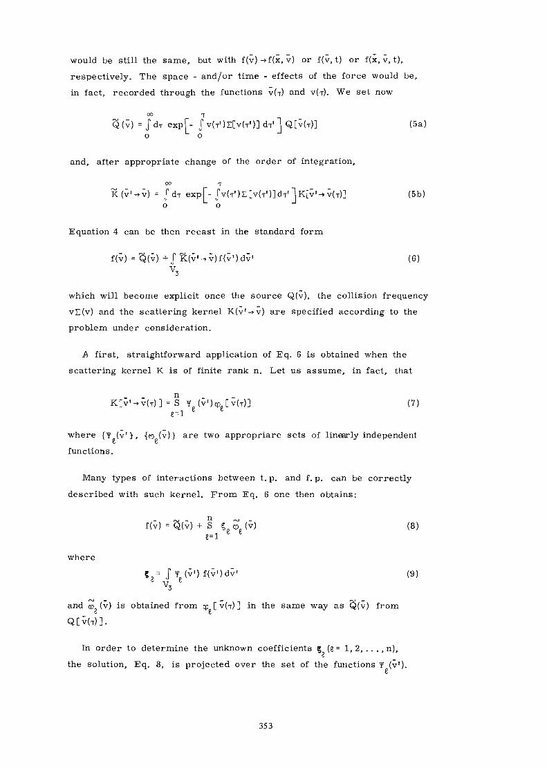
would be still the same, but with f (v ) -»f (x , v) or f(v, t) or f(x, v, t),

respectively. The space - and/or time - effects of the force would be,

in fact, recorded through the functions V(T) and V(T). We set now

OG f

Q(v) = J dT expf- J V(T')£[V(T')] dT11 Q[V(T)] (5a)o o

and, after appropriate change of the order of integration,

oo T

K(v ' -»v ) = JdT exp[- Jv(TI)E[v(T I)]dT

I lK[v'->v(T)] (5b)o o

Equation 4 can be then recast in the standard form

f(v) = Q(v) + J K ( v ' - > v ) f ( v ' ) d v ' (6)V3

which will become explicit once the source Q(v), the collision frequency

vZ(v) and the scattering kernel K(v'-»v) are specified according to the

problem under consideration.

A first, straightforward application of Eq. 6 is obtained when the

scattering kernel K is of finite rank n. Let us assume, in fact, that

K[V ' -»V(T) ] = S v ( V ' ) C P B [ V ( T ) ] (7)

where {¥ (v1) , {cp (v)} are two appropriare sets of linearly independentv O

functions.

Many types of interactions between t. p. and f. p. can be correctly

described with such kernel. From Eq. 6 one then obtains:

f (v) = Q(v) + S ç £ (v) (8)e=i

where

? = Jr ( v ' ) f ( v ' ) d v ' (9)K

and co (v) is obtained from cp [ V(T) ] in the same way as Q(v) from

Q[V(T)] .

In order to determine the unknown coefficients | (e = 1,2, . . . , n),\j

the solution, Eq. 8, is projected over the set of the functions V (v1)

353

Then the § 's are recognized to be in turn solutions to the system

of n linear algebraic equations

? e = § V ? m + B e (10)m=l

the matrix elements A and the known terms B of which being givenem i & &

by

and by

B = ff (v )<3(v )dv ( l ib)n d o * ' ^ * * 7 x '

respectively.

The field-dependent electrical conductivity can be derived from the

above formalism. If t. p. are taken to be electrons, multiplying both

sides of Eq. 8 by qv and integrating over the velocity domain V3, we

get for the total current density

Ï = I +q S g P v d v S (v) (12a)

where

Ï = q Jv Q(v)dv (12b)q

is the part contributed by the external source.

By introducing now Eq. 12 in Ohm's law

and setting E = ( l /q)F, there results

qi = a ( F ) F = q ï q+ q l i S g J " v c £ ( v ) d v . (13)

which gives the (nonlinear) electrical conductivity for a scattering kernel

of finite rank n. We notice that the electrical conductivity, as given by

Eq. 13, can be a rather complex function of E, the degree of complexity

depending on the choice of the two sets of functions y (v1) and CD (v).\i C

In general, one must, therefore, expect strong deviations from the linear

Ohm's law and then an anomalous behaviour of 5 as a function of E.

354

We recall, in fact, that both § and cp (v) on the r.h. s. of Eq. 13 areK £in general functions of the external field.

For isotropic scattering the kernel K depends only on the speeds

before and after the collision. In other words one has:

cpg (v) = cpg (v)

If the external force is directed along the z axis, that is F- v = F v

and, if we also make the change of variable

m . .

one obtains for the transform of cp (v) (Eq. 5a):G

V Vz z ._________ ,___~ - m r i r m n / ö ô T T / ^CD (v) = — exp - — / v^ + v^ +u ^ E ( v^ 8 F d L F d V x y v x-oo U J

(14)

• cp ( / V 2 + V 2 + U 2 ) duê V x y

which solves together with Eq. 13 the problem of the evaluation of

the electrical conductivity for an isotropic scattering kernel of finite

rank.

In the monodimensional case, that is when the dependence on v

and v disappears, then with v =v =0, Eq. 14 and 13 becomey x y

v vz zu ' £ ( u ' ) d u ' " ] c p ( u ) d u (15a)

J

and

(15b)

where k is the unit vector directed along the z axis.

Even if simpler than Eq. 13, the formulae, Eqs. 14 and 15, for the

electrical conductivity still retain a certain degree of complexity as a

function of E. We shall see later on that only for a particular choice

of the functions ¥ (v1) and cp (v) and in the limit of constant collision

frequency there is a case for which Eq. 14 will allow us to verify the

validity of Ohm's law. A general statement - which can be verified

through a standard expansion of the kernel K(v" -> v) in terms of F/m -

is that, for very weak fields and for sufficiently high cross-sections,

355

the total current is proportional to the field itself so that Ohm's law

is satisfied.

In the case when the kernel K [ V ' - > V ( T ) ] is not of finite rank,

different methods are available for solving Eq. 6 , and they are to be

chosen according to the structure of the resulting kernel K(v' ->v).

Among these methods we recall briefly the two following ones, both

of constructive type.

The first is the classical method of successive approximations,

which can be fruitfully applied when the calculation of the general

iterated kernel

K (v' •* v) = J K(v" -> v) K (v1 -> v") dv"T 7 ~

is sufficiently straightforward.

The second method worth mentioning consists in seeking for a

representation of the given kernel K(v ' -»v) of the type

~ - 0° r^>, n 0_ ^,, ^

where {^(v1)}, {cp'^v)} ( 6 = 1 , 2 , . . . ) are two denumerable complete

sequences of linearly independent functions belonging to an appropriate

class, and D . , (v ' -»v) is a kernel the norm of which can be made asn+1small as desired as n -> <=c. If, for a sufficiently large n, this latter

contribution can be neglected, then both the distribution function and

the electrical conductivity can be again built up through the model of a

scattering kernel of finite rank n. The use of either of the two construct-

ive methods recalled above will, of course, require a separate analysis

according to the physical kernel to be introduced in Eq. 6.

The extension of the theory to include spatial effects of the source is

immediate. In Eq. 4 f(v) is replaced by f(x, v). If the system of f. p.

fills the Euclidean space R3, the space Fourier transform of f (x, v)

is solution of Eq. 6 where <5 and K are now buckling dependent

(Boffi, 1978).

2.1. 2 Applicati£ns_

The first two applications concern the use of two scattering kernels,

as defined by Eq. 7, which are both separable (rank 1) and isotropic

in the laboratory system.356

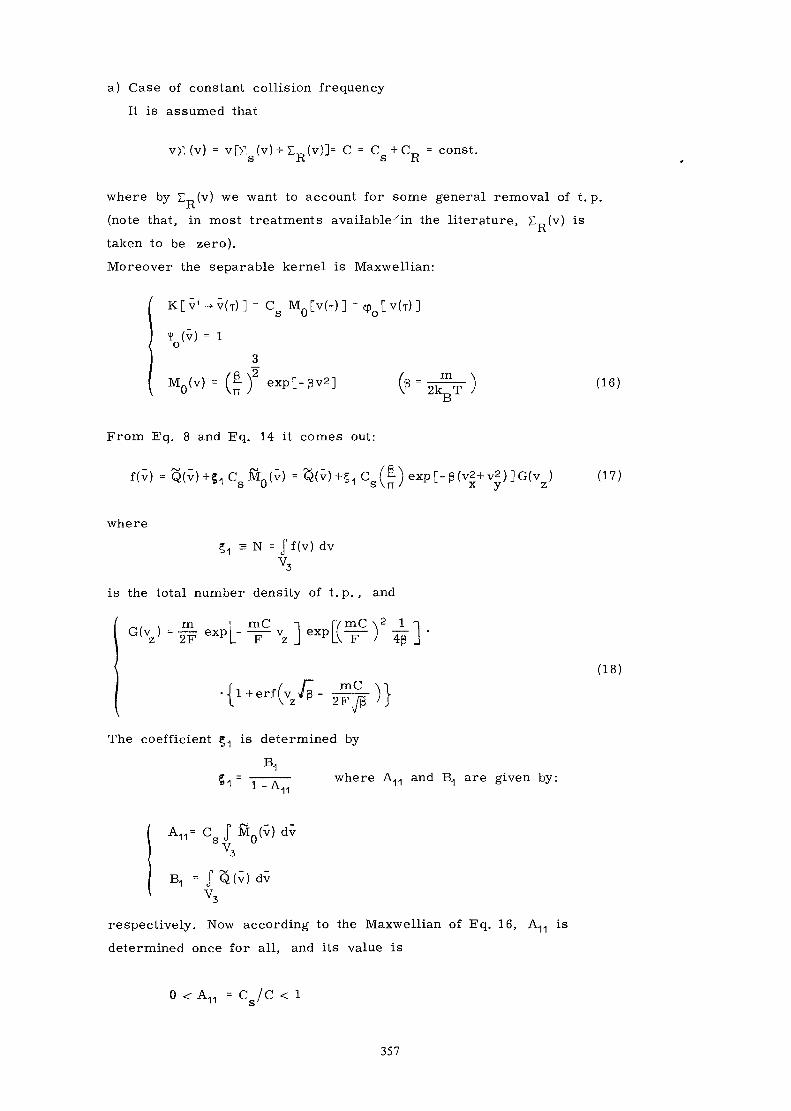
a) Case of constant collision frequency

It is assumed that

v E ( v ) = v[E (v) + E„(v}]= C = C +C = const.S K S ri

where by S,-, (v) we want to account for some general removal of t. p.K(note that, in most treatments availablexin the literature, E„(v) isRtaken to be zero).

Moreover the separable kernel is Maxwellian:

K[v ' -»V(T) ] =

¥ (v) = l

M0(v) = exp[-ßv2] m(16)

From Eq. 8 and Eq. 14 it comes out:

f(v) = §(v)+^C M (v) =o \ J

- s V T T , exp[ -ß(v2 + v2); (17)

where

Ç1 = N = J f (v ) dv

is the total number density of t. p., and

2 1

l + e r f ( v *\ zmC

The coefficient c^ is determined by

BIwhere A11 and B1 are given by:l -A .11

(18)

= c

B, = J Q(v) dvV3

respectively. Now according to the Maxwellian of Eq. 16,

determined once for all, and its value is

is

0 < A11 = C /C < 1

357

Turning to B1 , it can be verified that for different source spectra

the following common result holds:

B1 = QQ/4TTC > 0, where Qg is the source strength

so that

as expected from the conservation principle. If the external sourceis removed, we have to consider the eigenvalue problem. When

QQ -» 0, B1 -» 0 for the homogeneous equation associated to Eq. 10

( n = l ) to admit a nontrivial solution, it must be A^ = 1 or C_ = 0.

The density distribution is then given by

f ( v ) = ? 1 C

where §1 = N is a constant and G (v ) is the value of G(v ), Eq. 18,S Z Z

in the limit C-»C .s

f ^ \For a Maxwellian source (Q[v(r ) ] = -r- M..[V(T)] J the total currentdensity is from Eq. 13 ( n = l ) :

= f +Ï = k q ( J +J )= k —-M 'q s ^' q s' 4n mC2 V C-CS

Then Ohm's law is verified with

in which the dependence on C— is made explicit. In the homogeneousKcase with no removal (QQ, C_-*0) it is found that

as expected from the simplest form of the electron gas kinetic

theory (Qj, = 0).

b) Case of constant mean free path

For the collision frequency we assume that

vZ(v) = v[Z; _ ( v ) + Z (v) ]=(k 1 +k )|v = k |vö Jix Jt\ Z ^-

, k k2 = const.

358

The consistent separable Maxwellian kernel is then written as:

K[v'-»v(T)= ( |v' | ) ( k , | v ( T ) | M [v (T) ] )Z Z U Z

1/2with: M (v ) = (^ ) exp[-ßv2]

\J Z \ T / Z

This problem can be solved analytically as the previous one

(see réf. ). The unknown 51 is now given by

We stress the full analogy between these results and those obtained

for the case of constant collision frequency (Eq. 19).

Now we pass to study Ohm's law for the general case of

k1k > 0. For the total current density we have

XX

l+mk2 /2ßqE

indicating that Ohm's law is not satisfied. For the electrical conductivity

contributed by the scattering we get thus

= CT-'s, 0 l+(2ßq/mk2)E

with _

üs,0 4n mkR(k1+kR)2

as follows by recalling Eq. 21 for §1 .

One sees -with these two examples how the above formalism can be

applied to very different cases for which sometimes the Ohm's law is

no longer valid. If we do not restrict ourselves to analytic solutions

the proposed theory can be used to solve more general problems.The class of finite rank kernels K is sufficiently large to represent

very accurately many physical situations, but of course computer

program should be developed for this purpose.

2.2. T r a n s p o r t T h e o r y f o r C h a r g e d P a r t i c l e si n E l e c t r i c a n d M a g n e t i c F i e l d s(BOFFI.1979)

The above method can be easily extended to the case in which -

in addition to a constant electric field E - also the effects of a constant

magnetic field B must be taken into account.

359

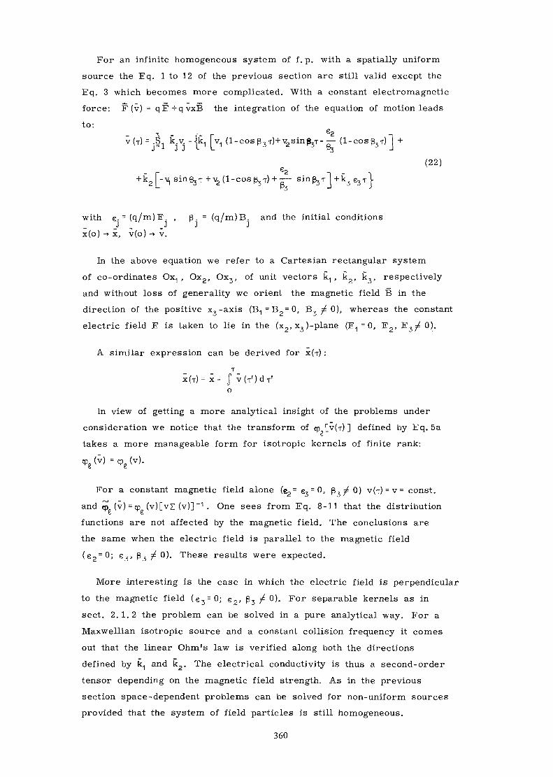
For an infinite homogeneous system of f . p. with a spatially uniform

source the Eq. 1 to 12 of the previous section are still valid except the

Eq. 3 which becomes more complicated. With a constant electromagnetic

force: E (v) = qË+qvxB the integration of the equation of motion leads

to:A - f- r ^ -\V ( T ) = . | k v -Jk, v1 (l-cosß3T)+v2sinß5T-— (I-COS^T) +

J J J ^ i - P 3 - J

(22)Go

T) + — sin^rl +k\, T \

with e. = (q/m)E. , ß. = (q/m)B. and the initial conditions

x(o) -» x, v(o) -» v.

In the above equation we refer to a Cartesian rectangular system

of co-ordinates Ox1 , Ox2, Ox3, of unit vectors k., , k2, k3, respectively

and without loss of generality we orient the magnetic field B in the

direction of the positive x3-axis (B 1 =B 2 =0, , B3 ^ 0), whereas the constant

electric field E is taken to lie in the (x2, x3)-plane (E1 = 0, E2, E3^ 0).

A similar expression can be derived for X(T) :

T

X ( T ) = x- J v (T ' )d i - 'o

In view of getting a more analytical insight of the problems under

consideration we notice that the transform of cp [V(T) ] defined by Eq. 5aG

takes a more manageable form for isotropic kernels of finite rank:

cpg (v) = cpe (v).

For a constant magnetic field alone (e2= e3

=0, ß3 ^ 0) V(T) = V= const.

and <p (v) = cp (v)[vZ (v)] ~1 . One sees from Eq. 8-11 that the distributiont t.,

functions are not affected by the magnetic field. The conclusions are

the same when the electric field is parallel to the magnetic field

( e 2 = 0 ; e3, ß3 ^ 0). These results were expected.

More interesting is the case in which the electric field is perpendicular

to the magnetic field ( e 3 = 0 ; e2, ß3 ^ 0). For separable kernels as in

sect. 2.1.2 the problem can be solved in a pure analytical way. For a

Maxwellian isotropic source and a constant collision frequency it comes

out that the linear Ohm's law is verified along both the directions

defined by k, and k2. The electrical conductivity is thus a second- order

tensor depending on the magnetic field strength. As in the previous

section space -dependent problems can be solved for non-uniform sources

provided that the system of field particles is still homogeneous.

360

More details and other applications can be found in references

(BOFFI, 1978, 1979).

3. AN APPLICATION OF TRANSPORT THEORY TO MATERIALS SCIENCE:ATOMIC MODEL FOR GRAIN BOUNDARY AND SURFACE DIFFUSION

Classical models for grain boundary diffusion (or surface diffusion)

of atoms are derived from the one proposed by Fisher (FISHER, 1951).

In these models, the grain boundary is viewed as a high diffusivity slab

of small but finite thickness 2 a (Fig. 8.3). The diffusion equation for

the concentration C(r, t) = C(x, y, t) is then solved, with appropriate

boundary conditions, in the composite medium made of this slab embedded

in the homogeneous bulk mate.rial (SUZUOKA, 1964).

The boundary conditions are:

C(x ,y ,0 ) = 6(y) D = D oxx = ± a + e

D'» D

x = ± a -

This type of model rises some questions:

i) Is the use of the diffusion equation justified in such a system ?

diffusion theory is known to be a poor approximation for short times

and close to the boundaries; its use in such a narrow medium as the grain

boundary is it reasonable ?

ii) What is the physical meaning of the grain boundary thickness

2a ?

3.1. T h e a t o m i c " t r a n s p o r t " m o d e l

In order to answer these questions, we propose a model nearer from

the actual situation. This model shall be an "atomic model", in which

the bicrystal is represented by a discrete set of points. The atoms jump

from point to point with appropriate jump frequencies. We then solve

the transport equation in this system, with boundary conditions similar

to those used by Suzuoka to solve the diffusion equation.

This atomic model has been established and developed at Saclay

(BENOIST, 1975). Its physical interest is to relate directly macroscopic

concentration profiles experiments to microscopic quantities such as

jump frequencies or number of fast transport paths.

361

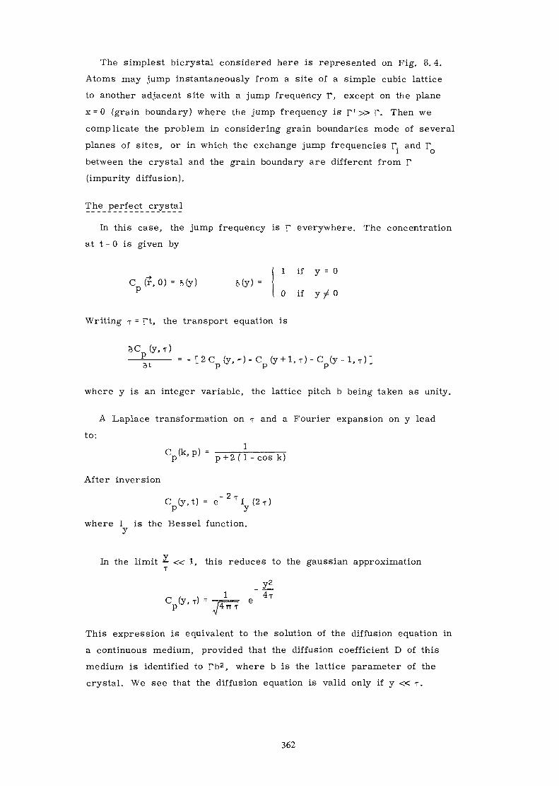
The simplest bicrystal considered here is represented on Fig. 8.4.

Atoms may jump instantaneously from a site of a simple cubic lattice

to another adjacent site with a jump frequency T, except on the plane

x = 0 (grain boundary) where the jump frequency is r' » F. Then we

complicate the problem in considering grain boundaries mode of several

planes of sites, or in which the exchange jump frequencies r. and r

between the crystal and the grain boundary are different from F

(impurity diffusion).

The perfect crystal

In this case, the jump frequency is r everywhere. The concentration

at t = 0 is given by

P

1 if y = 0, 0) = 6(y) 6 (y) =

0 if y ^ 0

Writing T = Ft, the transport equation is

(y,T)tT —— = - [ 2 C (y.o^ P

where y is an integer variable, the lattice pitch b being taken as unity.

A Laplace transformation on 7 and a Fourier expansion on y lead

to:

C (k,p) =V P + 2(1 -cos k)

After inversion

C (y,t) = e " 2 T I y ( 2 T )

where I is the Bessel function.y

In the limit — « 1, this reduces to the gaussian approximationT

This expression is equivalent to the solution of the diffusion equation in

a continuous medium, provided that the diffusion coefficient D of this

medium is identified to Fb2, where b is the lattice parameter of the

crystal. We see that the diffusion equation is valid only if y « T.

362

3.2. T h e s i m p l e s t b i c r y s t a l

The jump frequency is everywhere equal to r, except between the

sites of the grain boundary (x = 0), where it is r'»r. In order to

take conditions analogous to those of Suzuoka, we shall choose

C ( r , o ) = 6(y) + 6 (y + 1)

We are mainly interested by the quantity

-Cn(y,t) = V T T £ C C ( x , y , t ) - C (y , t ) ]

X=-oo

where C (y,t) is the concentration in a perfect crystal with the same

source; the quantity Cn may be obtained by experiments.

The general transport equation is, r and r1 being vectors with integer

components

The sum extends to the sites r1 nearest neighbours of r.

Practically we shall write this equation as we worked on a perfect

crystal with jump frequency r, but we shall add correction terms in

order to take into account the grain boundary. Writing T = Ft and1

3C(x.y.T) = _4C ( X ) y , T) + C(x + i j y )T) +oT

+ C(x ,y- l , T }+eo(x) [ -2C(0 ,y , T )

Let us make the Laplace -Fourier transformation

C(h.k.p) = dt e-* Y e-ikx e-ik^ C(x,y,T)^ U

X=-oo y=

and write

C(0,y , T ) = C0(y,T)

363

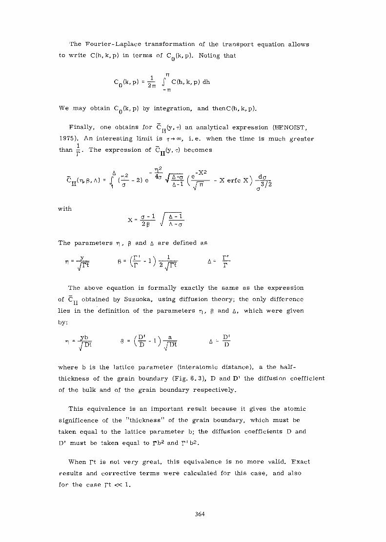
The Fourier-Laplace transformation of the transport equation allows

to write C(h, k, p) in terms of C (k, p). Noting that

Cn(k,P) =— J C(h,k,p) dhU ii TT

- TT

We may obtain C (k, p) by integration, and thenC(h, k, p).

Finally, one obtains for C (y, T) an analytical expression (BENOIST,

1975). An interesting limit is T-*°°, i.e. when the time is rauch greater

than —. The expression of CT_(y, T) becomes

Hda7^ -Xer fcx) -^V a

witha - 1 / A - lX = 2 ß V A - a

The parameters TJ , ß and A are defined as

r- y R - /H i \ * A -•~ ,/rt p VF / 2^

The above equation is formally exactly the same as the expression

of CTT obtained by Suzuoka, using diffusion theory; the only difference

lies in the definition of the parameters r\, ß and A, which were given

by:

7T5Î p - V D - - 1 ) ^ A = ^v v

where b is the lattice parameter (interatomic distance), a the half-

thickness of the grain boundary (Fig. 8. 3), D and D1 the diffusion coefficient

of the bulk and of the grain boundary respectively.

This equivalence is an important result because it gives the atomic

significence of the "thickness" of the grain boundary, which must be

taken equal to the lattice parameter b; the diffusion coefficients D and

D1 must be taken equal to Fb2 and f ' b 2 .

When Ft is not very great, this equivalence is no more valid. Exact

results and corrective terms were calculated for this case, and also

for the case Ft « 1.

364

3.3. G r a i n b o u n d a r y w i t h s e v e r a l p l a n e s o f s i t e s -I m p u r i t y d i f f u s i o n

The procedure above was generalized to a grain boundary with N

planes of sites. One finds that, at the limit Ft -> 0, the previous equation

still holds., provided the parameter ß is replaced by the parameter

ß' = Nß, i.e. the thickness of the grain boundary must be taken equal

to N lattice parameters b. Hence, a measure of the "thickness" of the

grain boundary by a profile concentration experiment is not the measure

of a geometrical quantity, but the measure of the number of fast transport

paths existing in this grain boundary.

In the case of impurity diffusion (r. ^ ?„ ^D, one shows that these

results are still valid in the limit rt-»°°, but with ß1 multiplied byr.

VMore complex configurations - The method_ of the correlation function

More complicated situations have been treated, in which the grain

boundary frequency jump r1, and the exchange frequencies r. and r„ , are

periodical along the y variable, and in which the grain boundary may have

a complex structure. Cases where the bicrystal is disorientated with

respect to the grain boundary have also been treated (Fig. 8 .5) . In any

case, the problem is to find a macroscopically equivalent simple bicrystal

of the type represented on Fig. 8.4. The calculation of these complex

situations is made possible by the use of the method of the correlation

function, which disconnects the problem of the grain boundary from the

problem of the outer crystal, writing the balance of currents between

the adjacent, sites of these two media. The correlation function G (y-»y,o

t - t 1 ) of the grain boundary is the probability fcr an atom entering the

grain boundary by the channel y" at time t1 to escape the grain boundary

by the channel y at time t. A similar definition holds for the correlation

function G (y1 -»y, t - t 1 ) of the crystal. By a convolution of these twocorrelation functions and the use of Fourier-Laplace transformation, it

is possible to rebuild the actual bicrystal and to treat, with some reason-

able approximations, rather complex configurations. This voluminous work

cannot find place here, one should refer to more detailed reports(BENÖIST, 1975).

365

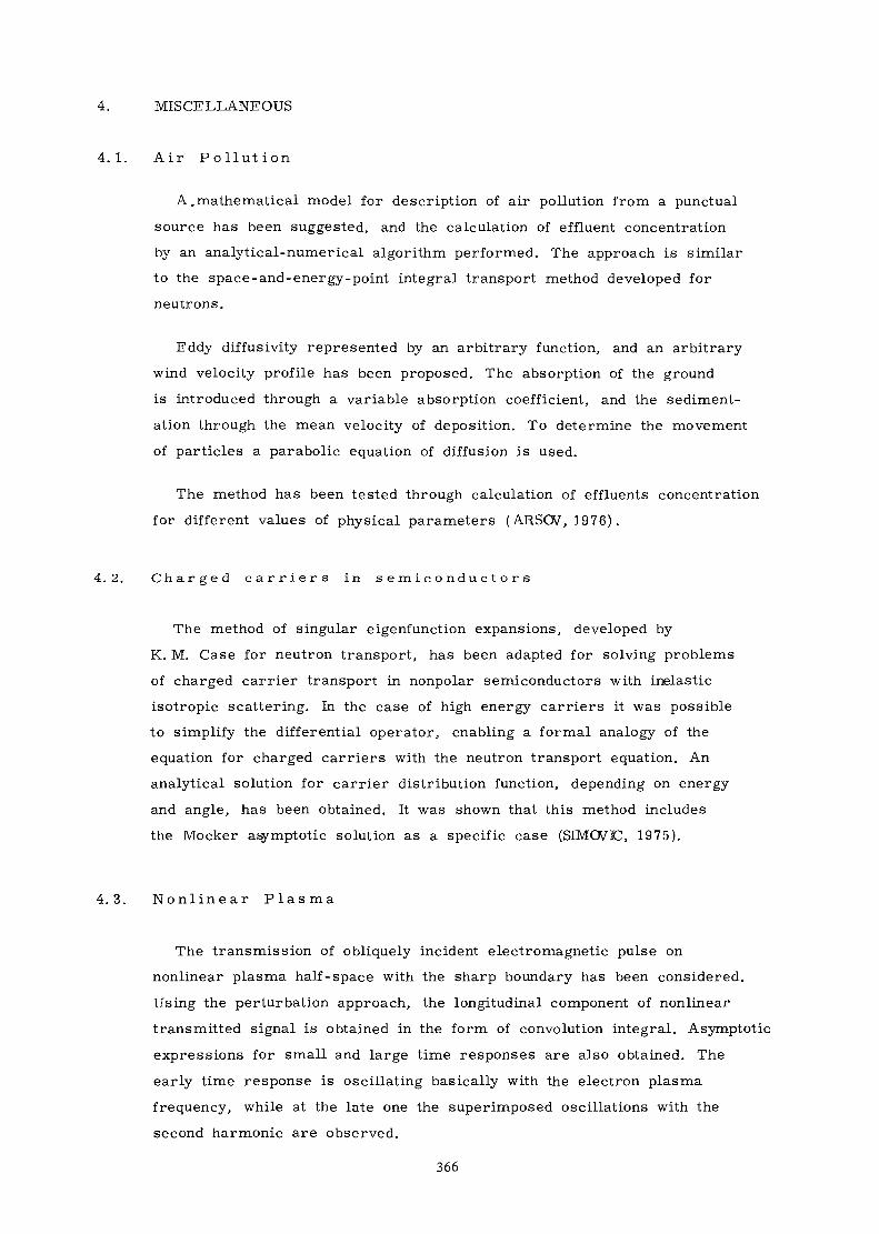
4. MISCELLANEOUS

4. 1. Air P o Hut ion

A .mathematical model for description of air pollution from a punctual

source has been suggested, and the calculation of effluent concentration

by an analytical-numerical algorithm performed. The approach is similar

to the space-and-energy-point integral transport method developed for

neutrons.

Eddy diffusivity represented by an arbitrary function, and an arbitrary

wind velocity profile has been proposed. The absorption of the ground

is introduced through a variable absorption coefficient, and the sediment-

ation through the mean velocity of deposition. To determine the movement

of particles a parabolic equation of diffusion is used.

The method has been tested through calculation of effluents concentration

for different values of physical parameters (ARSCV, 1976).

4.2. C h a r g e d c a r r i e r s i n s e m i c o n d u c t o r s

The method of singular eigenfunction expansions, developed by

K. M. Case for neutron transport, has been adapted for solving problems

of charged carrier transport in nonpolar semiconductors with inelastic

isotropic scattering. In the case of high energy carriers it was possible

to simplify the differential operator, enabling a formal analogy of the

equation for charged carriers with the neutron transport equation. An

analytical solution for carrier distribution function, depending on energy

and angle, has been obtained. It was shown that this method includes

the Mocker asymptotic solution as a specific case (SIMOVK, 1975).

4.3. N o n l i n e a r P l a s m a

The transmission of obliquely incident electromagnetic pulse on

nonlinear plasma half-space with the sharp boundary has been considered.

Using the perturbation approach, the longitudinal component of nonlinear

transmitted signal is obtained in the form of convolution integral. Asymptotic

expressions for small and large time responses are also obtained. The

early time response is oscillating basically with the electron plasma

frequency, while at the late one the superimposed oscillations with the

second harmonic are observed.

366

The above hydrodynamic model has been compared with the kinetic

approach (based on Vlasov transport equation), and the results have shown

to be the same (STANK, 1978).

REFERENCES

ARSOV Lj.S., Analytical-numerical method for treatment of turbulentdiffusion of particles in the air, Tehnicka Fizika, Journal ofEngineering Physics, XIV, (1976), 5-17

APPERT, K. et al: Two dimensional Quasilinear Evolution of the ElectronBeam Plasma Instability, Physical Review Letters, 37 (1976), 502

BENOIST P. , MARTIN G. - Atomic Model for Grain Boundary and SurfaceDiffusion, Thin Solid Films, 25, 181 (1975)

BENOIST P. - Bases Théoriques du Modèle Atomique de Diffusion Inter-granulaire - CEA Report (Saclay). To be published.

BENOIST P., MARTIN G. - Modèle Atomique de Diffusion Inter granulaire:Généralisation - Journal de Physique, Colloque C 4, suppl. auno. 10, tome 36 (1975)

BOFFI V. C. and MOLINARI V. G. - Intégral Boltzmann Equation in théStudy of Diffusion of Test Particles: Nuovo Cimento, 34B,345 (1976)

BOFFI V.C. , MOLINARI V. G. and WONNENBERGER W. - Theory ofNonlinear Electrical Conductivity via Integral Boltzmann Equation:Nuovo Cimento, 45B, 109 (1978)

BOFFI V.C. , MOLINARI V. G. - Integral Transport Theory for ChargedParticles in Electric and Magnetic Fields: Nuovo Cimento, 49B,77 (1979)

COOPER G. E., Deflection of Fast Ions in a Plasma, Lawrence LivermoreLaboratory, Report UCID-16157 (1970)

CORMAN E.G. et al T Nucl. Fusion 1_5 (1975)

DAVIDSON R. C. : Methods in Nonlinear Plasma Theory, New York:Academic Press 1972

FISHER J.C. - J. Appl. Phys., 22_, 74 (1951)

GOLDSTEIN H., In Aspects of Reactor Shielding, Addison-WesleyPublishing Comp. (1959) p. 172, 265

HALDY P. -A., LIGOU J. - A Moment Method for Calculating theTransport of Energetic Charged Particles in Hot Plasmas -Nucl. Fusion 17, 6 (1977)

HALDY P. -A. - Energy Deposition of Fast Ion Beams in Plasmas -To be published (1979)

367

HUFFMAN T. J. et al - Sputtering Calculations with the Discrete-OrdinatesMethod, Nucl. Sei. Eng. 6£, 204 (1978)

LIGOU J., HALDY P. -A. - Energy Deposition of Fast Ions in Plasmas,Atomkernenergie, Bd 32 (1978)

LIGOU J. and CALINON R. - Recent Development of Methods for theCalculation of Turbulent Electron Beam Plasma Interactions -Atomkernenergie, Bd 32 (1978)

LIGOU J. - The Importance Factor of a Source in Neutron Kinetics -Nucl. Sei. and Eng. 66 (1978)

LIGOU J. - Neutron Kinetics of Highly Compressed Fissionable Pellets -Nucl. Sei. and Eng. ^3_ (1977)

LIGOU J. - Discrete and Continuous Interactions in Charged ParticleTransport Theory - To be published in Nucl. Sei. Eng. (1979)

LIGOU J. L. - Comment on "Laser fusion hydrodynamics calculations",Letter to the Editor, Nucl. Sei. Eng. 55_ (1978)

MOSES G. A. - Laser Fusion Hydrodynamics Calculations, Nucl. Sei.Eng. 64 (1977)

SHEARER J.W. Nucl. Fusion JL5 (1975)

SIMOVIC R. - The Solution of Transport Equation of High Energy ChargedCarriers in Nonpolar Semiconductors by Singular EigenfunctionMethod, MSc Thesis, Faculty of Electrical Engineering,University of Belgrade (1975)

SPENCER L. V. - Phys. Rev. 9^ (1955)

STANIC B.V. and MILANOVIC Dj. R. - Transmission of TransientElectromagnetic Plane Wave Obliquely Incident on NonlinearPlasma Half-Space, Contributed Papers, IX SPIG, Dubrovnik,28 Aug.-2 Sept. 1978, 317-320

SUZUOKA T. - J. Phys. Soc. Japan, 1£, 839 (1964)

VEDENOV A.A. , RYUTON D.D. - Reviews of Plasma Physics,Consultant Bureau, New York, 6 (1975), 1-76

VELARDE, G. et al - Development of Methods for Time Dependent Neutronicand Hydrodynamic Calculation with Feedback of Laser-Fission-Fusion Systems (p. IV-12). Presented at the International Workshop-Thinkshop on Advanced Nuclear Energy System Analysis - Graz,Austria, March 29-31 (1978)

368

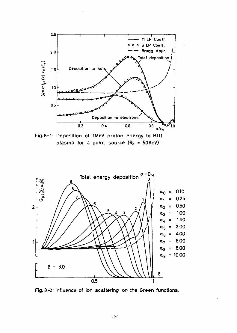
Deposition to electronst t

Fig.8-1: Deposition of 1MeV proton energy to BDTplasma for a point source (0e = SOKeV)

1.0

T . . . ...Total energy deposition

1-

0,5 1

Fig. 8-2: Influence of ion scattering on the Green functions.

369

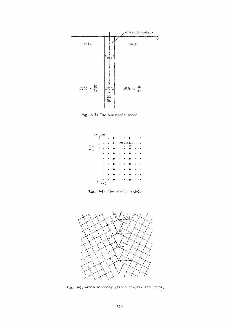
Bulk

DV'C - |£3t

2

:D'X

Grain boundary____ ________________ _ ___________ -k..

a

r

3C3t

/ XBulk

DV2C = ~

Fig. 8-3: The SuzuoKa's model

r.r.

Fig. 8-4: The atomic model.

\>^\>\L

Fig. 8-5: Grain boundary with a complex structure.

370

HOW TO ORDER IAEA PUBLICATIONSAn exclusive sales agent for IAEA publications, to whom all orders

and inquiries should be addressed, has been appointedin the following country:

UNITED STATES OF AMERICA UNIPUB, 345 Park Avenue South, New York, NY 10010

In the following countries IAEA publications may be purchased from thesales agents or booksellers listed or through yourmajor local booksellers. Payment can be made in localcurrency or with UNESCO coupons.

ARGENTINA

AUSTRALIABELGIUM

CZECHOSLOVAKIA

FRANCE

HUNGARY

INDIA

ISRAEL

ITALY

JAPANNETHERLANDS

PAKISTANPOLAND

ROMANIASOUTH AFRICA

SPAIN

SWEDEN

UNITED KINGDOM

U.S.S.R.YUGOSLAVIA

Comisiôn Nacional de Energi'a Atomica, Avenida del Libertador 8250,RA-1429 Buenos AiresHunter Publications, 58 A Gipps Street, Collingwood, Victoria 3066Service Courrier UNESCO, 202, Avenue du Roi, B-1060 BrusselsS.N.T.L., Spélenà 51, CS-113 02 Prague 1Alfa, Publishers, Hurbanovo nemestie 6, CS-893 31 BratislavaOffice International de Documentation et Librairie, 48, rue Gay-Lussac,F-75240 Paris Cedex 05Kultura, Hungarian Foreign Trading CompanyP.O. Box 149, H-1389 Budapest 62Oxford Book and Stationery Co., 17, Park Street, Calcutta-700 016Oxford Book and Stationery Co., Scindia House, New Delhi-110 001Heiliger and Co., Ltd., Scientific and Medical Books, 3, Nathan StraussStreet, Jerusalem 94227Libreria Scientifica, Dott. Lucio de Biasio "aeiou".Via Meravigli 16, 1-20123 MilanMaruzen Company, Ltd., P.O. Box 5050, 100-31 Tokyo InternationalMartinus Nijhoff B.V., Booksellers, Lange Voorhout 9-11, P.O. Box 269,NL-2501 The HagueMirza Book Agency, 65, Shahrah Quaid-e-Azam, P.O. Box 729, Lahore 3Ars Polona-Ruch, Centrala Handlu Zagranicznego,Krakowskie Przedmiescie 7, PL-00-068 Warsawllexim, P.O. Box 136-137, BucarestVan Schaik's Bookstore (Pty) Ltd., Libri Building, Church Street,P.O. Box 724, Pretoria 0001Diaz de Santos, Lagasca 95, Madrid-6Diaz de Santos, Balmes 417, Barcelona-6AB C.E. Fritzes Kungl. Hovbokhandel, Fredsgatan 2, P.O. Box 16356,S-103 27 StockholmHer Majesty's Stationery Office, Agency Section PDIB, P.O.Box 569,London SE1 9NHMezhdunarodnaya Kniga, Smolenskaya-Sennaya 32-34, Moscow G-200Jugoslovenska Knjiga, Terazije 27, P.O. Box 36, YU-11001 Belgrade

Orders from countries where sales agents have not yet been appointed andrequests for information should be addressed directly to:Division of PublicationsInternational Atomic Energy AgencyWagramerstrasse 5, P.O. Box 100, A-1400 Vienna, Austria

TRANSPORT THEORY AND ADVANCED REACTOR ...

Documents