Transport in the subtropical lowermost stratosphere during the Cirrus Regional Study of Tropical Anvils and Cirrus Layers–Florida Area Cirrus Experiment

Transport in the subtropical lowermost stratosphere during the Cirrus

Regional Study of Tropical Anvils and Cirrus Layers–Florida Area

Cirrus Experiment

Jasna V. Pittman,1,2 Elliot M. Weinstock,1 Robert J. Oglesby,3 David S. Sayres,1

Jessica B. Smith,1 James G. Anderson,1 Owen R. Cooper,4,5 Steven C. Wofsy,1

Irene Xueref,1,6 Cristoph Gerbig,1,7 Bruce C. Daube,1 Erik C. Richard,8

Brian A. Ridley,9 Andrew J. Weinheimer,9 Max Loewenstein,10 Hans-Jurg Jost,11,12

Jimena P. Lopez,11 Michael J. Mahoney,13 Thomas L. Thompson,8

William W. Hargrove,14 and Forrest M. Hoffman14

Received 28 July 2006; revised 17 October 2006; accepted 21 November 2006; published 20 April 2007.

[1] We use in situ measurements of water vapor (H2O), ozone (O3), carbon dioxide(CO2), carbon monoxide (CO), nitric oxide (NO), and total reactive nitrogen (NOy)obtained during the CRYSTAL-FACE campaign in July 2002 to study summertimetransport in the subtropical lowermost stratosphere. We use an objective methodology todistinguish the latitudinal origin of the sampled air masses despite the influence ofconvection, and we calculate backward trajectories to elucidate their recent geographicalhistory. The methodology consists of exploring the statistical behavior of the data byperforming multivariate clustering and agglomerative hierarchical clustering calculationsand projecting cluster groups onto principal component space to identify air masses of likecomposition and hence presumed origin. The statistically derived cluster groups are thenexamined in physical space using tracer-tracer correlation plots. Interpretation of theprincipal component analysis suggests that the variability in the data is accounted forprimarily by the mean age of air in the stratosphere, followed by the age of the convectiveinfluence, and last by the extent of convective influence, potentially related to the latitudeof convective injection (Dessler and Sherwood, 2004). We find that high-latitudestratospheric air is the dominant source region during the beginning of the campaign whiletropical air is the dominant source region during the rest of the campaign. Influence ofconvection from both local and nonlocal events is frequently observed. The identificationof air mass origin is confirmed with backward trajectories, and the behavior of thetrajectories is associated with the North American monsoon circulation.

Citation: Pittman, J. V., et al. (2007), Transport in the subtropical lowermost stratosphere during the Cirrus Regional Study of

Tropical Anvils and Cirrus Layers–Florida Area Cirrus Experiment, J. Geophys. Res., 112, D08304, doi:10.1029/2006JD007851.

1. Introduction

[2] In order to predict the response of the global climatesystem to thermal and chemical changes resulting from

forcing by infrared-active species, it is necessary to under-stand the mechanisms that transport air masses between thetroposphere and the stratosphere year-round. Transport ofchemical constituents plays a crucial role in explainingissues such as UV dosage at the surface, distribution ofgreenhouse gases like water vapor and carbon dioxide in theupper troposphere and lower stratosphere (UT/LS), and

JOURNAL OF GEOPHYSICAL RESEARCH, VOL. 112, D08304, doi:10.1029/2006JD007851, 2007

1Departments of Earth and Planetary Sciences and of Chemistry andChemical Biology, Harvard University, Cambridge, Massachusetts, USA.

2Now at NASA Marshall Space Flight Center, Huntsville, Alabama,USA.

3Department of Geosciences, University of Nebraska, Lincoln,Nebraska, USA.

4Cooperative Institute for Research in Environmental Sciences,University of Colorado, Boulder, Colorado, USA.

5Also at Earth System Research Laboratory, NOAA, Boulder, Colorado,USA.

6Now at Laboratoire des Sciences du Climat et de l’Environment,Commissariat l’Energie Atomique, Gif-Sur-Yvette, France.

7Now at Max Planck Institute for Biogeochemistry, Jena, Germany.

Copyright 2007 by the American Geophysical Union.0148-0227/07/2006JD007851

D08304

8Earth System Research Laboratory, NOAA, Boulder, Colorado, USA.9Atmospheric Chemistry Division, National Center for Atmospheric

Research, Boulder, Colorado, USA.10NASA Ames Research Center, Moffett Field, California, USA.11Bay Area Environmental Research Institute, Sonoma, California,

USA.12Now at NovaWave Technologies, Redwood City, California, USA.13Jet Propulsion Laboratory, California Institute of Technology,

Pasadena, California, USA.14Oak Ridge National Laboratory, Oak Ridge, Tennessee, USA.

1 of 23

heterogeneous ozone loss in the tropopause region. Thesummertime circulation, particularly in the stratosphere, hasbeen studied less extensively than the other seasons, be-cause it has been regarded as quiescent because of theweakening of the large-scale circulation driven by thermalforcing and wave activity [Plumb, 2002]. Several studies,however, have shown that this season can be important,because deep convection over land can have a direct andsignificant impact on the chemical composition of theextratropical lower stratosphere [Jost et al., 2004; Desslerand Sherwood, 2004].[3] In this study, we use an Eulerian approach to quali-

tatively explore transport pathways in the subtropical low-ermost stratosphere during the summer by (1) using a novelcombination of nonparametric and parametric techniquesalong with tracer-tracer correlations to identify the origin ofsampled air masses and (2) backward trajectory calculationsto elucidate the responsible transport pathways. For thispurpose, we use in situ measurements of H2O, O3, CO2,CO, NO, and NOy, obtained aboard NASA’s WB-57 aircraftduring the Cirrus Regional Study of Tropical Anvils andCirrus Layers–Florida Area Cirrus Experiment (CRYSTAL-FACE) that was based out of Key West, Florida during July2002.[4] Earlier observations of H2O vapor [Brewer, 1949] and

O3 [Dobson, 1956] in the stratosphere revealed the exis-tence of a large-scale meridional circulation that couples the

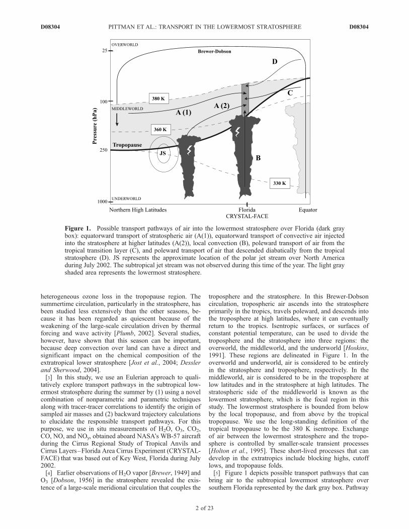
troposphere and the stratosphere. In this Brewer-Dobsoncirculation, tropospheric air ascends into the stratosphereprimarily in the tropics, travels poleward, and descends intothe troposphere at high latitudes, where it can eventuallyreturn to the tropics. Isentropic surfaces, or surfaces ofconstant potential temperature, can be used to divide thetroposphere and the stratosphere into three regions: theoverworld, the middleworld, and the underworld [Hoskins,1991]. These regions are delineated in Figure 1. In theoverworld and underworld, air is considered to be entirelyin the stratosphere and troposphere, respectively. In themiddleworld, air is considered to be in the troposphere atlow latitudes and in the stratosphere at high latitudes. Thestratospheric side of the middleworld is known as thelowermost stratosphere, which is the focal region in thisstudy. The lowermost stratosphere is bounded from belowby the local tropopause, and from above by the tropicaltropopause. We use the long-standing definition of thetropical tropopause to be the 380 K isentrope. Exchangeof air between the lowermost stratosphere and the tropo-sphere is controlled by smaller-scale transient processes[Holton et al., 1995]. These short-lived processes that candevelop in the extratropics include blocking highs, cutofflows, and tropopause folds.[5] Figure 1 depicts possible transport pathways that can

bring air to the subtropical lowermost stratosphere oversouthern Florida represented by the dark gray box. Pathway

Figure 1. Possible transport pathways of air into the lowermost stratosphere over Florida (dark graybox): equatorward transport of stratospheric air (A(1)), equatorward transport of convective air injectedinto the stratosphere at higher latitudes (A(2)), local convection (B), poleward transport of air from thetropical transition layer (C), and poleward transport of air that descended diabatically from the tropicalstratosphere (D). JS represents the approximate location of the polar jet stream over North Americaduring July 2002. The subtropical jet stream was not observed during this time of the year. The light grayshaded area represents the lowermost stratosphere.

D08304 PITTMAN ET AL.: TRANSPORT IN THE LOWERMOST STRATOSPHERE

2 of 23

D08304

A corresponds to equatorward transport of high-latitudestratospheric air (HLS). This pathway can carry either purestratospheric air that descended diabatically from the over-world at high latitudes (pathway A(1)), or a mixture withtropospheric air that was injected into the stratosphere viamiddle- or high-latitude convection (pathway A(2)). Path-way B corresponds to direct penetration of local convection.Pathway C corresponds to poleward isentropic transport ofair from the Tropical Tropopause Layer (TTL) across thesteeply sloped subtropical tropopause. In this study, weadopt the definition of the TTL presented by Gettelmanand Forster [2002], which is the region bounded from belowby the level of neutral buoyancy (340 to 350 K) and fromabove by the cold-point tropopause (380 to 390 K). PathwayD corresponds to isentropic transport from the tropical lowerstratosphere (TLS) followed by diabatic descent into thesubtropical lowermost stratosphere.[6] Several studies have reported evidence of each one of

these transport pathways in the UT/LS at various locationsand times using measurements of different chemical tracers.For instance, analysis of ozone profiles during CRYSTAL-FACE showed layers of higher ozone in the subtropicallowermost stratosphere resulting from large-scale equator-ward transport of high-latitude air into the subtropics(pathway A(1)) [Richard et al., 2003]. Summertime obser-vations showed tropospheric air reaching into the lowermoststratosphere via convection (pathway A(2) and B) [Poulidaet al., 1996; Vaughan and Timmis, 1998; Jost et al., 2004;Ray et al., 2004]. Late spring in situ aircraft measurements[Dessler et al., 1995; Hintsa et al., 1998] as well asmodeling studies [Chen, 1995; Dethof et al., 2000; Stohlet al., 2003] have provided evidence for poleward isentropictransport of air from the TTL (pathway C). Last, a combi-nation of satellite and aircraft measurements of ozoneshowed that diabatic descent into the lowermost strato-sphere (pathway D) can happen during the summer, thoughit is strongest during late winter and early spring [Prados etal., 2003].[7] The methodology followed in this study consists of

three stages. The first stage consists of objectively cluster-ing the data set and identifying the dominant modes ofvariability by performing a statistical analysis in threedifferent steps. In the first step, we use a nonparametric,nonhierarchical clustering technique to construct six dimen-sional clusters based on in situ measurements of H2O, O3,CO2, CO, NO, and NOy obtained in the subtropical lower-most stratosphere during CRYSTAL-FACE. In the secondstep, we perform nonparametric agglomerative hierarchicalclustering to group the clusters based on similarities to eachother in their chemical characteristics. In the third step, wedo a parametric Principal Component Analysis (PCA) inwhich we project the data set onto its first three eigen-vectors. We plot the results, color coded by group assign-ment, in order to examine the cluster groups in a spacecomposed of the most relevant modes of variability in thedata set. This three-step statistical analysis has been appliedpreviously to identify distinct tropical convective profilesusing the vertical structure information obtained fromvarious measurements from the Tropical Rainfall MeasuringMission (TRMM) [Boccippio et al., 2005]. The secondstage consists of identifying the source regions by compar-ing the mean mixing ratios of the six chemical tracers in

each cluster with reference values for each source regionand demonstrating consistency in air mass origin betweenthe statistically derived results and the physically basedtracer-tracer correlation plots. The third and final stageconsists of calculating backward trajectories in order toinvestigate the recent geographical history of the air massesultimately sampled in the subtropical lowermost strato-sphere. The trajectories are also used to confirm the iden-tification of source regions obtained in the second stage. Wewill show that the monsoon circulation over North Americais critical in order to explain not only the origin but alsothe elevated humidity observed of the air sampled inthe lowermost stratosphere during CRYSTAL-FACE. AsDunkerton [1995] pointed out, monsoon circulation can bean important driver of horizontal and vertical transport ofair reaching the UT/LS region when atmospheric waveactivity is otherwise weak. This study strongly supportsthat conclusion.[8] The paper is structured as follows. Section 2 explains

the usefulness of the chemical tracers chosen and describesthe data sets used in this study. Section 3 describes thestatistical techniques, tracer-tracer correlations, and trajec-tory model. Section 4 discusses the results obtained fromapplying the methodology described in section 3. Section 5summarizes the major findings of this study.

2. Data

2.1. Chemical Tracers

[9] We use six different chemical tracers in this study,namely H2O, O3, CO2, CO, NO, and NOy. These tracers arechosen because they can provide the following informationand discrimination in the lowermost stratosphere, our regionof interest. H2O can distinguish wet, convectively influ-enced air from otherwise very dry stratospheric air. O3,while having a significant gradient between the troposphereand the stratosphere, can also provide information on themean age of stratospheric air: older stratospheric air hashigher mixing ratios than younger stratospheric air. CO2 canalso provide valuable information on the age of air, since itsmixing ratio is affected by both the positive secular trendobserved in the atmosphere and its seasonal cycle. CO,when found at high concentrations, is a good indicator ofthe presence of recently injected tropospheric air into thelowermost stratosphere, since it is produced primarily in thetroposphere by human activity such as biomass burning. NOis the most unequivocal evidence of recently injectedconvective air when found at higher mixing ratios thanbackground levels, since its main source in the UT/LS islightning. Last, NOy, which represents the sum of allreactive nitrogen species (NOy = NO + NO2 + NO3 +2N2O5 + HNO3 + peroxyacetyl nitrate (PAN) + . . .), canprovide information on the altitudinal and latitudinal originof air, as the tracer increases with increasing altitude andlatitude, and along with NO, it can provide information onthe age of the convective intrusion into the stratosphere. Inthis study, we use NOy measurements in the gas phase only.The use of all these tracers together will ultimately allow usto distinguish a larger variety of air masses more clearly byexploiting the unique information that each tracer canprovide.


3 of 23

D08304

[10] In addition to the above information obtained fromeach chemical tracer, the chemical lifetimes of these tracersallow us to separate observed changes in mixing ratios dueto chemistry from changes due to transport. All tracersexcept NO have chemical lifetimes ranging from severalmonths to several years in the lower stratosphere. NOx

(= NO + NO2) has a chemical lifetime of about 1 week inthe UT/LS during the summer [Ridley et al., 1996]. OnceNO is produced by lightning, the partitioning of NOx willfavor NO during the day because of photolysis of NO2.Therefore observations of high NO in the UT/LS during theday would be indicative of the presence of tropospheric airthat was lofted by strong convection. A recent study showedthat large enhancements in NO (up to 50 times larger thanbackground values) were indeed observed duringCRYSTAL-FACE and that they were associated with light-ning activity from local thunderstorms and possibly trans-port from the boundary layer [Ridley et al., 2004]. For theremaining tracers, observed changes in mixing ratios duringthe campaign are more likely the result of changes intransport, which can happen in timescales shorter than thetracers’ chemical lifetimes.

2.2. CRYSTAL-FACE

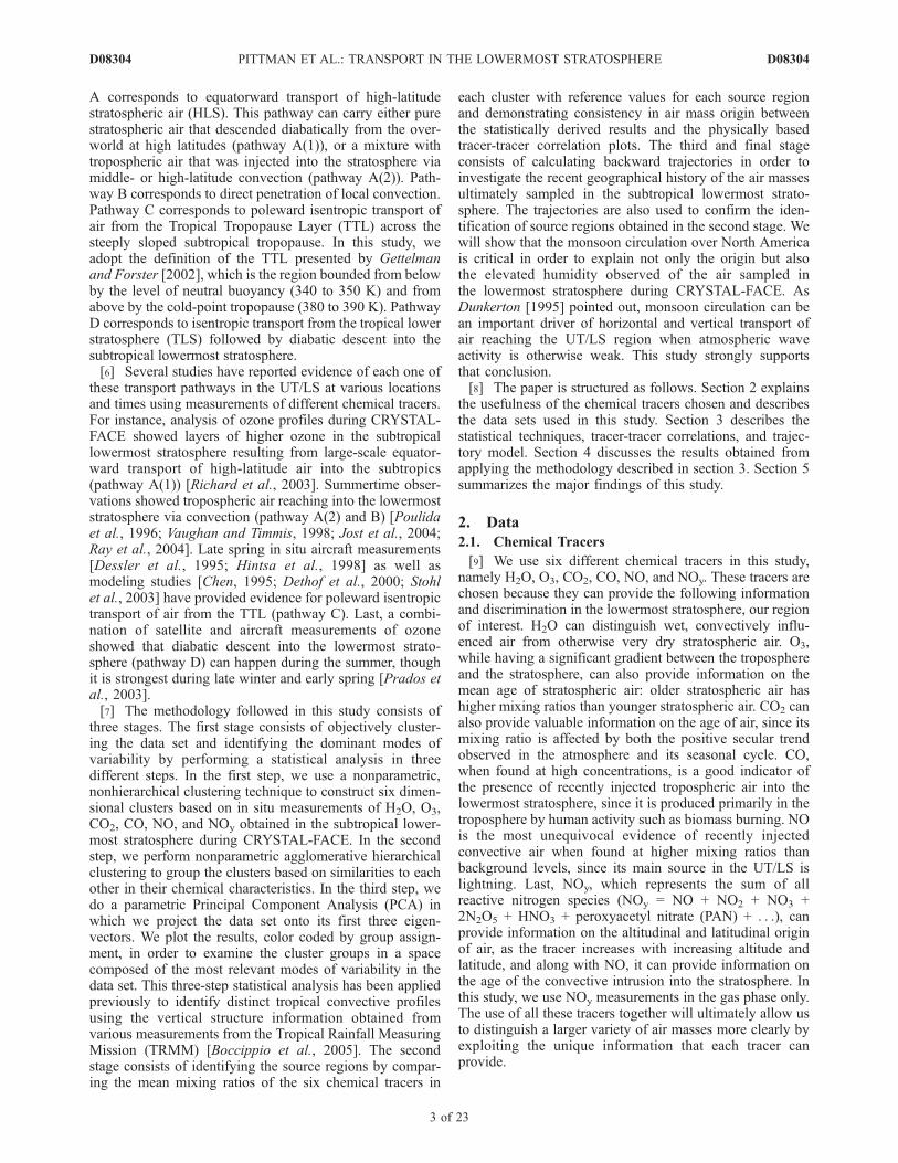
[11] CRYSTAL-FACE was based out of Key West, Flor-ida and included 12 flights over 27 days from 3 to 29 July2002, excluding the two ferry flights between Houston, TXand Key West, FL [Jensen et al., 2004]. We restrict ouranalysis to data collected in the lowermost stratosphere overthe southern Florida region between 24�N and 27�N and77�Wand 85�Was shown in Figure 2. We exclude the flightof 29 July from this analysis because of the existence of twotropopauses: one at approximately 12 km, which was over2 km below the average location of the local tropopause and

another at approximately 16 km, which was coincident withthe location of the 380-K isentrope during this campaign.The variability in the location of the tropopause throughoutthis flight made it difficult to specify the boundaries for thelowermost stratosphere.[12] The tracer measurements used are: H2O measured by

Lyman-a photofragment fluorescence using the Harvardhygrometer, with a ±5% uncertainty [Weinstock et al.,1994], O3 measured by dual-beam UV absorption, with a±3% uncertainty [Proffitt and McLaughlin, 1983], NO andNOy measured by catalytical reduction of NOy to NOfollowed by detection of NO through the chemilumines-cence reaction with O3, with an uncertainty of ±(7% +15 pptv) for NO and ±(9% + 15 pptv) for NOy [Ridley et al.,1994], CO measured by mid-IR absorption using a tunablediode laser, with a ±3% uncertainty [Loewenstein et al.,2002], and CO2 measured by nondispersive IR absorption,with a ±0.1 ppmv uncertainty [Daube et al., 2002]. All theseinstruments flew on NASA’s WB-57F. The tracer dataanalyzed in this study are averaged over 10 s giving ahorizontal resolution of 1.8 km on average along theWB-57’s flight track. Only observations that reported meas-urements for all of the six chemical tracers are considered.Because of the large spatial and temporal range of valuesmeasured for these tracers during the campaign, none of theabove measurement uncertainties are significant enough tocompromise the conclusions of this study.[13] We use the location of the local tropopause reported

by the Microwave Temperature Profiler (MTP) instrument[Denning et al., 1989]. This instrument uses the WorldMeteorological Organization (WMO) definition of the tro-popause as the lowest level at which the lapse rate (�dT/dz)decreases to 2 K/km or less, and the average lapse ratewithin the next 2 km does not exceed 2 K/km. Location of

Figure 2. Geographical location of all aircraft campaigns used in this study.


4 of 23

D08304

the local tropopause using in situ measurements of pressureand temperature made by the pressure-temperature instru-ment, which has uncertainties of 0.1 hPa and 0.5 K[Thompson and Rosenlof, 2003], and application of theWMO definition yielded results that agreed well with thosereported by MTP.[14] We restrict this analysis to clear-air data sampled in

the lowermost stratosphere. Using calculated saturationwater vapor mixing ratios obtained from in situ pressureand temperature measurements and in situ ice water meas-urements obtained from the Harvard Total Water and theHarvard Water Vapor instruments, we identify and removeoccasional cloud data sampled in our region of interest.Consequently, all references to H2O in this study are to H2Oin the vapor phase only. For the lower boundary of thelowermost stratosphere, we use the local tropopause ob-served during each flight. The location of the local tropo-pause varied from a minimum potential temperature of360 K (14.4 km or 147 hPa) to a maximum of 365 K(15.6 km or 121 hPa). For the upper boundary of thelowermost stratosphere, we use the tropical tropopausecorresponding to the 380-K isentrope, which was found tobe between 15.2 km (127 hPa) and 16.2 km (110 hPa) oversouthern Florida during the campaign.

2.3. Source Regions

[15] In order to put the CRYSTAL-FACE measurementsin context, we use in situ measurements from three previousaircraft campaigns. These are: Stratospheric Tracers ofAtmospheric Transport (STRAT) based out of Californiain July 1996 and out of Hawaii in August 1996, Photo-chemistry of Ozone Loss in the Arctic Region in Summer(POLARIS) based out of Fairbanks, Alaska in July 1997,and Clouds and Water Vapor in the Climate System(CWVCS) based out of Costa Rica in August 2001. Specificlocations of these campaigns are shown in Figure 2. TheSTRAT data are used to obtain reference values for tropicalsource regions and to investigate circulation in the strato-sphere on the west side of the monsoon. The POLARIS andCWVCS data are used to obtain reference values for thepossible high-latitude and tropical source regions for airtransported into the subtropical lowermost stratosphere viathe pathways shown in Figure 1.

[16] The majority of the tracer measurements obtainedduring these campaigns were made by the same instruments(with attendant uncertainties) used during CRYSTAL-FACE. A few measurements, however, were obtained fromdifferent instruments. During the STRAT and POLARIScampaigns, NO and NOy were measured by the NOAAAeronomy Laboratory reactive nitrogen instrument [Faheyet al., 1989] with uncertainties of ±(6% + 4 pptv) for NOand ±(10% + 100 pptv) for NOy, and CO was measured bythe Aircraft Laser Infrared Absorption Spectrometer[Webster et al., 1994] with a ±5% uncertainty. DuringCWVCS, O3 was measured by the Harvard ozone instru-ment instead [Weinstock et al., 1986]. All instruments flewaboard NASA’s ER-2 during STRAT and POLARIS, andaboard NASA’s WB-57 during CWVCS.[17] The tracers used in this study, except for CO2, do not

have significant trends in the stratosphere that can compro-mise the conclusions of this study. While the spatialcoverage of the in situ aircraft data is limited, severalstudies have shown consistent correlations in the strato-sphere of long-lived tracers such as O3, CO2, NOy, and N2Ocollected during aircraft campaigns that took place atdifferent latitudes and longitudes between 1987 and 1997and excellent agreement between aircraft measurements andoutput from chemical transport models [Murphy et al.,1993; Fahey et al., 1996; Strahan et al., 1998; Strahan,1999]. This consistency and level of agreement serve asevidence that measured tracer-tracer correlations show littlelongitudinal dependence, and can be used to representdifferent latitudinal regions of the stratosphere. On the basisof the results from these studies, we create reference tablesfor each source region, and we check for consistency withmeasured tracer-tracer correlations and climatologies [seeStrahan, 1999; Richard et al., 2003]. We do not findcompromising departures between our reference profilesand the climatologies that can have a significant effect onour results. The location and ranges of tracer mixing ratiosfor the source regions used in this study are reported inTables 1 and 2, respectively.[18] In addition to in situ aircraft data, we also use surface

measurements provided by NOAA’s Climate Monitoringand Diagnostics Laboratory Carbon Cycle and GreenhouseGases (CMDL CCGG) group. In particular, we use CO2

measurements collected at various locations in the tropics

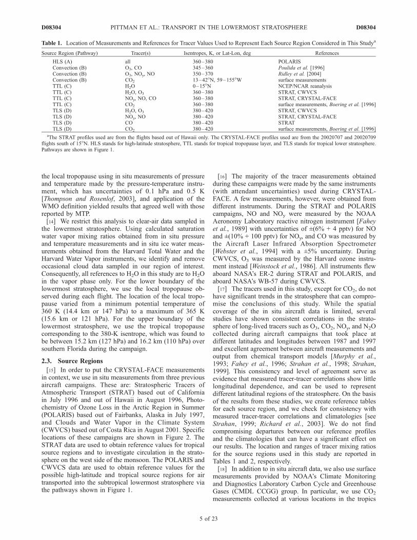
Table 1. Location of Measurements and References for Tracer Values Used to Represent Each Source Region Considered in This Studya

Source Region (Pathway) Tracer(s) Isentropes, K, or Lat-Lon, deg References

HLS (A) all 360–380 POLARISConvection (B) O3, CO 345–360 Poulida et al. [1996]Convection (B) O3, NOy, NO 350–370 Ridley et al. [2004]Convection (B) CO2 13–42�N, 59–155�W surface measurementsTTL (C) H2O 0–15�N NCEP/NCAR reanalysisTTL (C) H2O, O3 360–380 STRAT, CWVCSTTL (C) NOy, NO, CO 360–380 STRAT, CRYSTAL-FACETTL (C) CO2 360–380 surface measurements, Boering et al. [1996]TLS (D) H2O, O3 380–420 STRAT, CWVCSTLS (D) NOy, NO 380–420 STRAT, CRYSTAL-FACETLS (D) CO 380–420 STRATTLS (D) CO2 380–420 surface measurements, Boering et al. [1996]

aThe STRAT profiles used are from the flights based out of Hawaii only. The CRYSTAL-FACE profiles used are from the 20020707 and 20020709flights south of 15�N. HLS stands for high-latitude stratosphere, TTL stands for tropical tropopause layer, and TLS stands for tropical lower stratosphere.Pathways are shown in Figure 1.


5 of 23

D08304

and midlatitudes. The mixing ratios reported in Table 2 areadjusted or estimated in order to account for this tracer’ssecular trend and seasonal cycle in the atmosphere. In thecase of POLARIS data, we adjust the 1997 measurements towhat they would be in 2002 using the secular trend of1.5 ppmv/year. For the tropical source regions, we estimatethe mixing ratios using the mean monthly averaged surfacemeasurements at Mauna Loa and Samoa and the transporttimes through the TTL and the tropical lower stratosphereobserved by Boering et al. [1996].[19] Because tropospheric H2O is very variable, it is

difficult to provide constraints for the contribution of thistracer from the troposphere. Instead of relying on previousmeasurements, we calculate saturation mixing ratios usingthe Clausius-Clapeyron equation and tropopause pressureand temperature obtained from the National Centers forEnvironmental Prediction/National Center for AtmosphericResearch (NCEP/NCAR) Reanalysis data set. A warm biasin NCEP/NCAR tropical temperatures was accounted for bysubtracting 2 K from the temperature field [Shah and Rind,1998]. The reported H2O values for the TTL source regionshown in Table 2 correspond to the minimum and maximumsaturation mixing ratios at the local tropopause between theequator and 15�N and 0� and 180�W during July 2002. Inconvective sources, H2O can vary by one or two orders ofmagnitude, which makes it difficult to constrain. The actualcontribution of H2O vapor from a convective source iscontrolled by various factors, such as temperature where iceparticles from the convective system detrain, strength of theconvection, and microphysical conditions. Because of thelarge variability, we do not provide a specific range inTable 2.

3. Methodology

3.1. Statistical Analysis

[20] The statistical analysis is carried out in three steps.The goal of the first step is to identify ‘‘natural’’ groupingsof the data set based on the chemical composition of the airmasses using methods that do not rely on prior knowledgeor constraints. For this purpose, multivariate cluster analysisis performed on clear-air observations in the lowermoststratosphere. Each air mass observation consists of six tracermeasurements, which serve as the six coordinates in dataspace. Since tracer mixing ratios are reported in differentunits, we use standardized anomalies instead of the actualmixing ratios for each tracer value. The standardized anom-aly is calculated by subtracting the mean value for thecampaign from each observation and dividing this differ-ence by the standard deviation. Multivariate clusters arecreated using the k-means method, which is nonparametric

and nonhierarchical [Hargrove and Hoffman, 2004;Hoffman et al., 2005]. Briefly, in this method the onlyparameter chosen a priori is k, the number of clusters, andno other a priori knowledge is used. The procedure startswith a set of k seed centroids that are delineated in principalcomponent space to obtain a reasonable first guess. Thesecentroids are a widely distributed subset of the observationsand the final results do not depend on the initial guesses. Inthe first pass, every observation in PC space is assigned tothe closest centroid. Then at the end of the pass, the centroidposition is recomputed to be the mean of each coordinate ofall of the observations classified to that centroid. A newiteration starts using the recomputed centroids. This iterativeprocess continues until fewer than 0.5% of the observationschange cluster assignment from the last iteration. At thispoint, the group assignment has been stabilized and theclassification process has converged. The fact that clustersare independently redefined at each new iteration makes thismethod nonhierarchical. The main criterion used for theselection of k is based on the distribution of the data amongthe clusters. Ideally, clusters should contain neither toomany nor too few observations. We tested various valuesfor k, namely 5, 15, and 20, to produce an acceptabledistribution. We found k = 15 to give the best distributionof number of observations among clusters.[21] The goal of the second step is to explore the

similarities and differences among the 15 clusters. For thispurpose, we perform agglomerative clustering, which isnonparametric but hierarchical [Wilks, 2006]. Similar tothe multivariate clustering, this method also uses standard-ized anomalies instead of actual mixing ratios. In thistechnique, we use the Euclidean metric to calculate dis-tances between observations in the n-dimensional space (inour case n = 6). The six-dimensional space where thedistances are calculated is composed of the standardizedanomalies for each of the six tracers. We will refer to thisspace as the tracer space. When clusters contain more thanone observation, several schemes can be used to determinethe actual distance between two clusters (groups of obser-vations). The most common schemes are: single-linkage ifthe distance is the minimum distance between an observa-tion from one cluster and an observation from the othercluster, average-linkage if the distance is the averagedistance between all possible pairs of observations in thetwo clusters, and complete-linkage if the distance is themaximum distance between an observation from one clusterand an observation from the other cluster. We tested thesethree linkage schemes, and we found that all approachesyielded essentially the same underlying structure. Wechoose the complete linkage scheme, since it is based ona more stringent criterion for grouping clusters [cf. Wilks,

Table 2. Representative Values of Trace Gases From Each of the Four Source Regions Considered in This Studya

Source Region (Pathway) H2O, ppmv O3, ppbv CO2, ppmv CO, ppbv NO, pptv NOy, pptv

HLS (A) 10–4 300–600 370.5–368.7 35–21 250–170 2000–2800Convection (B) 10s–100s 60–120 369–374.5 80–140 100–2000 200–4000TTL (C) 12–4.8 40–160 373.8–372.8 70–45 150–400 200–1300TLS (D) 9–4.5 150–400 373.4–371.4 45–25 250–500 500–1500

aAll ranges except the ones for the convective source are listed as observed values at the bottom of the region followed by observed values at the top ofthe region. Each region is specified in Table 1. The CO2 ranges in the TTL and TLS represent the extreme values from the seasonal cycle of this tracerwithin each source region. These values might not necessarily occur at the edges of these source regions. Pathways are shown in Figure 1.


6 of 23

D08304

2006, p. 552]. Once the distances between all clusters havebeen determined, we perform the agglomerative hierarchicalclustering. This is an iterative process where at each step thepair of clusters (or groups of clusters) that reside the closestto each other in the six-dimensional tracer space are merged.This process of creating new groups at each step iscontinued until all clusters are eventually merged into onegroup (i.e., the original data set). The results of the agglom-eration are presented in a tree diagram, or dendrogram,illustrating the hierarchy of the sets of groups. In thedendrogram, clusters that are closer to each other in tracerspace, indicating that they share similar tracer mixing ratios,show up as members of the same branch of the tree. Clusterswith similar tracer mixing ratios could be associated withsimilar origins.[22] The goal of the third step is to provide context for

the interpretation and understanding of the clusteringresults. For this, we use PCA, which is a parametricapproach. In this technique, the eigenvalues and eigen-vectors of a correlation matrix constructed using thestandardized anomalies of a data set are calculated [Wilks,2006]. In our case, the data set consists of the original,nonclustered air mass observations obtained throughoutthe campaign, where each observation is composed of sixtracer measurements. The eigenvectors represent the or-thogonal modes of variability in the data and theircorresponding eigenvalues give the relative importanceof each eigenvector. The first eigenvector explains thelargest mode of variability, and each successive eigen-vector explains the next largest mode of variability notaccounted for by previous eigenvectors. Eigenvectors arecommonly referred to as empirical orthogonal functions(EOFs) when they characterize spatial patterns of vari-ability at specific points in time. Since at each point intime, our data set contains only one observation in space,to avoid confusion we will simply refer to them aseigenvectors rather than EOFs. Of the six eigenvectorsobtained using this technique, the first three are kept,since their eigenvalues account for 93% of the totalvariance (51%, 28%, and 14%, respectively). Sub-sequently, we calculate the principal component timeseries for each of the three eigenvectors, which we willsimply refer to as PC1, PC2, and PC3, respectively. Wecalculate each PC by summing the product of thestandardized anomalies of the data and the correspondingeigenvector over all six tracers for each air mass obser-vation obtained during the campaign. Hence these timesseries represent the temporal evolution throughout the cam-paign of the contribution of each eigenvector (or modeof variability) to the total variance. We then plot theseorthogonal PCs against each other and color code eachelement of the PC on the basis of the cluster group assign-ment of the observation that it represents [Boccippio et al.,2005]. This approach allows us to explore the behavior ofthe cluster groupings in the context of independent modesof variability in the data.

3.2. Tracer-Tracer Correlations

[23] Plumb and Ko [1992] showed that long-lived tracershave compact and nearly linear correlation plots in thestratosphere with a slope reflecting the influence of sourcesand sinks. Correlation plots have been used effectively in

previous studies to help distinguish air originating fromdifferent source regions [Hintsa et al., 1998; Hoor et al.,2002; Ray et al., 2004].[24] In this study, we analyze correlation plots of

different tracers with respect to H2O for several reasons.This tracer has a strong gradient across the tropopausewith low values in the stratosphere and high values (oneto three orders of magnitude larger) in the troposphere,thereby allowing us to identify convectively injected airinto the stratosphere. H2O has a lifetime of 100 years inthe lower stratosphere [Brasseur and Solomon, 1986]making it a good tracer for large-scale transport. Thistracer has a well documented seasonal cycle and astratospheric source. On an annual basis, seasonalchanges in stratospheric H2O over the tropics closelytrack the saturation mixing ratios set by the temperaturesof the tropical tropopause [Mote et al., 1996; Weinstock etal., 2001]. The main stratospheric source of H2O isoxidation of CH4. For every molecule of CH4 destroyed,two molecules of H2O are produced and this contributionis obvious in air masses that have spent more than3.8 years in the stratosphere and are located north of20�N and above 440 K [Dessler et al., 1994; Hurst et al.,1999]. For a timescale equivalent to the period of thecampaign, changes in H2O due to the seasonal cycle andCH4 oxidation can be neglected.[25] In addition to analyzing tracers versus H2O

(tracer:H2O) correlation plots, we also analyze CO2:O3

and NOy:O3 plots. These three tracers are long-lived andexhibit significant vertical and latitudinal gradients in thestratosphere. Both O3 and NOy increase with increasinglatitude and altitude in the lower stratosphere whereas CO2

decreases with increasing latitude. Therefore correlationplots using these tracers can provide latitude and altitudeinformation of potential source regions.[26] On the basis of our current understanding of sources

and sinks in the troposphere and stratosphere, we expect tofind the following tracer-tracer correlations of air masses inthe stratosphere. NO:H2O and CO:H2O should show posi-tive correlations, because all these tracers are mainly pro-duced in the troposphere and all of them are then removedby different mechanisms (e.g., dehydration, photolysis,chemistry) once the air reaches the stratosphere. NOy:O3

should also show a positive correlation, because thesetracers are both lower in the troposphere and higher in thestratosphere where they are produced as a result of photo-lysis and chemistry. O3:H2O and NOy:H2O should shownegative correlations instead, because while the troposphereis a major source for H2O, O3 and NOy are mainlygenerated in the stratosphere except for the case of tropo-spheric convection where lightning can be a significantsource of NOy (via NOx production). The correlations ofCO2 versus other tracers in tropospheric air can be compli-cated by the seasonal cycle of CO2 and its differenttropospheric sources (e.g., maritime versus continental,tropics versus high latitudes). For stratospheric air,CO2:O3 should show a negative correlation, where CO2 isdecreasing in older air because of its secular trend whileO3 is increasing because of photochemical production. TheCO2:H2O correlation is further complicated by the seasonalcycle of H2O and convection into the UT/LS. In general, alltracer:H2O correlations can breakdown in the presence of


7 of 23

D08304

convective air, because convection does not have a uniqueeffect on H2O.

3.3. Trajectory Model

[27] Backward trajectories for selected flights during theCRYSTAL-FACE campaignare calculated using the For-ward and Backward trajectory (FABtraj) model that hasbeen verified against satellite imagery, trace gas measure-ments and the widely used FLEXTRA model [Cooper et al.,2004a]. The model has been used for studying air masstransport through synoptic-scale midlatitude cyclones andfor simulating air mass transport within the lower strato-sphere and stratospheric intrusions [Cooper et al., 2004b].[28] The FABtraj model is a diabatic model that uses

NCEP Final Analyses (FNL) wind fields and a linearinterpolation scheme in space and time. The meteorologicaldata set used is available every 6 hours and has a horizontalgrid resolution of 1� � 1� and a vertical resolution of21 levels between 1000 and 100 hPa. The vertical levelsare prescribed in sigma (or terrain-following) coordinates.Vertical motion in the FABtraj model is driven solely by thevertical wind component of the FNL analyses, which isundefined at pressures lower than 100 hPa. This constrainton vertical motion at low pressures, however, does notcompromise the conclusions of our study, because it affectsonly a very small number of trajectories (e.g., 1 out of 196initialized on 16 July and 6 out of 80 initialized on 23 July).Convection is therefore not parameterized and it is notresolved in subgrid scale in this model. The effects ofconvection, however, are parameterized in the FNL.[29] Summertime convection can be strong enough to

transfer air masses from the troposphere into the strato-sphere, a process that involves crossing of isentropes. Giventhe location and the season of CRYSTAL-FACE, we chooseto use a trajectory model that allowed this crossing insteadof using adiabatic trajectories. Additionally, air masses thatare advected back in time for more than 2–3 days are verylikely to experience changes in temperature during thesummer, especially when traveling over or through regionsof strong and frequent convective activity over land. Thiscondition affects the entropy of the air mass and makes itstrajectory nonadiabatic.

4. Results and Discussion

4.1. Source Region Identification

[30] Table 2 shows reference values for the six chemicaltracers used in this study in each of the four possible sourceregions identified in Figure 1. Each source region can bequalitatively identified on the basis of (1) the correlations ofchemical tracer abundance observed in Table 2 (e.g., hightracer 1 and low tracer 2 in source A) and (2) ourunderstanding of sources and sinks described in section 3.2.[31] We will show next how different tracers can help

discriminate different source regions. Older stratospheric aircoming from high latitudes (pathway A in Figure 1) isclearly characterized by higher O3 and NOy, and lower CO2.When this air is not contaminated by convection, H2O, CO,and NO are expected to be low. Younger stratospheric aircoming from tropical latitudes, on the contrary, is charac-terized by lower O3 and NOy, and higher CO2 (pathways Cand D in Figure 1). Similarly, when not contaminated by

convection, H2O, CO, and NO are expected to be low butCO and NO would be higher than in nonconvective olderstratospheric air. Convective air found in the lowermoststratosphere is clearly characterized by higher H2O (path-way B in Figure 1). Good indicators of recent convectiveinjection into the UT/LS region (i.e., less than 1 week oldbecause of the chemical lifetime of NO) are higher CO, NOand NOy (driven by higher NO). Convective injection intothe UT/LS region older than a week will be characterized byelevated H2O and possibly CO, and low NO due to itschemical loss over time.

4.2. Statistical Analysis

[32] The multivariate clustering technique is used toconstruct 15 distinct clusters based on the six chemicaltracers chosen for this study. Figure 3 shows the centroidvalues and ranges for each tracer and each cluster. Thisclustering technique attempts to minimize multivariate var-iability and construct clusters with clear and unique inter-pretations. In some cases, however, we might find thecluster interpretation to be ambiguous. Therefore it isimportant to examine and consider not only the centroidvalues themselves, but also the range and distribution ofvalues of all cluster members relative to the centroid value.This point will be important later on when we explain thecontents of Table 4.[33] The results of the agglomerative clustering are sum-

marized in the dendrogram shown in Figure 4. To the rightof the dendrogram, the percent occurrence of each clusterbased on the air masses sampled by the aircraft during thecampaign is presented. The closer the clusters are in tracerspace (x axis in Figure 4a), the more similarities theseclusters share in terms of tracer values and hence presumedorigin, and vice versa. The largest distance is found to bebetween cluster 15 (or C15) and the remaining clusters.According to the results shown in Figure 3, this cluster canbe easily and uniquely identified as air dominated by recentconvection based on the highest mixing ratios of NO. As wedecrease the distance in tracer space in the dendrogram (i.e.,move to the left along the x axis), we notice the emergenceof new branches. These different branches suggest theexistence of structure in the data. The dashed vertical lineis plotted at a distance where five distinct branches occur.Those branches or groupings are color coded as follows:group 1 or G1 (with C2, C9, C3, C8, C4, and C7) is codedyellow, G2 (with C6, C10, C11, C1, and C12) is codedgreen, G3 (with C5 and C14) is coded black, G4 (with C13)is coded red, and G5 (with C15) is coded blue (see Figure 4).This classification will constitute the basis for the analysispresented from this point forward. Groups G1 and G2 bothcontain a relatively large number of clusters; the dendro-gram suggests these can also be divided into subgroups bymoving even farther to the left along the x axis. Thesubgroups within each group presumably share similarorigins, but we will show how their distinctions are basedon subtle but important differences in the fractional con-tributions of the dominant source regions and in some cases,the altitudinal location of the clusters.[34] The grouping of clusters presented in Figure 4 is the

result of the complete linkage agglomerative hierarchicalclustering scheme chosen. The main difference betweenthese results and the ones obtained using other linkage


8 of 23

D08304

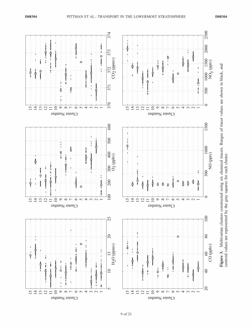
Figure

3.

Multivariate

clustersconstructed

usingsixchem

ical

tracers.Ranges

oftracer

values

areshownin

black,and

centroid

values

arerepresentedbythegraysquares

foreach

cluster.


9 of 23

D08304

schemes is in the membership of C13 and C14. Thedifferent calculation details forced these clusters to changebranches. This result implies that these clusters have some-what ambiguous origins. As will be shown later, these twoclusters are made up of members that appear to havediffering origins.[35] Before examining the five groups of clusters in PC

space, we deduce a physical interpretation for each of theunderlying eigenvectors (hence PCs) shown in Table 3using the qualitative description of source regions describedin section 4.1. The coefficients of these vectors constitutethe weight given to each tracer in the calculation of the PCs.In eigenvector 1, the largest positive weights are given to O3

and NOy and the largest negative weight is given to CO2,suggesting that this eigenvector denotes how old on averagestratospheric air is. In eigenvector 2, the largest weights, allpositive, are given to H2O, CO, and NO, suggesting that thiseigenvector denotes how recent convective influence is.Last in eigenvector 3, the largest positive weight is givento H2O and the largest negative weight is given to NO,suggesting that this eigenvector denotes how large and/orold convective influences are. While mathematically possi-ble, the large negative NO anomalies required for oldconvective influence should not physically occur. Instead,this weight reflects the many small negative anomalies thatrepresent the background NO values to which aged con-vective air will relax.[36] Figures 5–7 show the vertical profiles of each of the

tracers with shading based on the sign of the PC. Figure 5shows the tracer profiles for PC1. Consistent with theinterpretation of eigenvector 1, PC1 denotes the ‘‘meanage of air in the stratosphere.’’ When a PC1 value ispositive, the air mass observed at that time corresponds toolder air presumably originating from higher latitudes in the

stratosphere, and when the value is negative, the air masscorresponds to younger stratospheric air presumably origi-nating from tropical latitudes. Because of the small coef-ficients for H2O and NO in eigenvector 1, both old andyoung air masses appear to have varying extents of con-vective influence. Figure 6 shows the tracer profiles forPC2. Consistent with the interpretation of eigenvector 2,PC2 denotes the ‘‘age of the convective influence.’’ Whena PC2 value is positive, the observed air mass at that timecorresponds to recent convection, and when the value isnegative, the air mass corresponds to older convection.Besides an apparent, and not unreasonable, altitude prefer-ence of positive PC2 values for lower altitudes, the othertwo tracers, O3 and CO2, have small coefficients in eigen-vector 2 implying that there is little correlation between theage of the convective influence and the mean age ofstratospheric air. Figure 7 shows the tracer profiles for PC3.Consistent with the interpretation of eigenvector 3, PC3denotes the ‘‘extent of convective influence.’’ When aPC3 value is positive, the air mass observed at that timecorresponds to greater and/or older convective influence,and when the value is negative, the air mass corresponds tosmaller convective influence. The negative PC sign of thefew large NO values associated with a known recentconvective event exemplifies the mathematical peculiarity

Figure 4. (a) Agglomerative hierarchical clustering of the 15 multivariate clusters. The distancebetween clusters is calculated in tracer space. The vertical line shown at 6.5 is used to analyze thebranches found at this distance. The branches or groups are color coded as shown in the figure.Subgroups are found within G1 and G2 and their distinctions are explained in the text. (b) Percentoccurrence of each cluster sampled in the lowermost stratosphere during CRYSTAL-FACE. Thisdistribution shows that 15 is an appropriate number of clusters.

Table 3. Coefficients of the Three Eigenvectors Used in This

Analysisa

Eigenvector H2O O3 CO2 CO NO NOy

1 �0.0271 0.5548 �0.5533 �0.3067 0.1084 0.52872 0.5044 �0.0901 �0.0452 0.5520 0.5978 0.27093 0.7853 0.1796 �0.0301 �0.0200 �0.5872 �0.0709

aEach coefficient constitutes the weight given to each tracer in thecalculation of the PCs shown in Figures 6–8.


10 of 23

D08304

Figure

5.

Verticalprofilesofthesixchem

ical

tracersusedin

this

studyshaded

onthebasis

ofthesignofPC1.Gray

diamondsareforpositivePC1,andblack

circlesarefornegativePC1.ThisPCisinferred

asrepresentingthemeanageof

airin

thestratosphere.

See

textforadetailedexplanationoftheinference.


11 of 23

D08304

Figure

6.


ical

tracersusedin

this

studyshaded

onthebasis

ofthesignofPC2.Gray


circlesarefornegativePC2.ThisPC

isinferred

asrepresentingtheageofthe

convectiveinfluence.See



12 of 23

D08304

Figure

7.


ical

tracersusedin

this

studyshaded

onthebasis

ofthesignofPC3.Gray


circlesarefornegativePC3.ThisPCisinferred

asrepresentingtheextentofthe

convectiveinfluence,whichcanberelatedto

thelatitudeoftheconvectiveinputfollowingresultsfrom

Dessler

and

Sherwood[2004].See



13 of 23

D08304

noted above for eigenvector 3. The other tracers, O3, CO2,CO and NOy, have small coefficients in eigenvector 3implying that there is little correlation between the extentof convective influence and the age of the convection andthe mean age of stratospheric air. When removing the airmasses with high NO caused by recent convection andconsequently the resulting extreme negative values for PC3,the magnitude and sign of PC3 in the remaining air massesare highly dominated by H2O only (correlation coefficientof 0.93). The more positive the standardized anomaly forH2O is, the larger the value for PC3 is. In a recent study,Dessler and Sherwood [2004] argued that the impact ofconvective injection on stratospheric H2O is higher athigher latitudes. They attributed this connection to warmertemperatures, lower relative humidity, and a larger ‘‘con-vective contrast’’ (i.e., difference in tracer concentrationbetween the convective outflow and the local environment)in the midlatitude stratosphere compared to the tropics. Wewill use their argument to extend the physical interpretationof PC3 as follows: positive values, which are driven bypositive anomalies in H2O, correspond to a larger extent ofconvective influence and presumed latitudes of convectiveinjection northward of southern Florida where the convec-tive contrast is larger, and vice versa.[37] We next examine the five groups of clusters in PC

space. The reason for doing this is to look at the correspon-dence between clusters and PCs in the context of thedominant modes of variability in the data set. This approachis somewhat analogous to the more physically based tracer-tracer correlations, but in this case we use a statisticalframework instead. The results are shown in Figure 8.[38] On the basis of the physical meaning deduced for the

underlying eigenvectors of each PC using tracer mixingratios, and the location of each cluster group in PC spaceshown in Figure 8, we find the following results. G1 is high-latitude stratospheric air mixed with various amounts ofolder convective air except for a few members in the C4–C7 couplet that show more recent and larger convectiveinfluence from events that presumably occurred at northernlatitudes, G2 is tropical air (from the tropopause layer or thelower stratosphere) mixed with various amounts of olderconvective air, and in some cases even older convective airthan G1, from events both north and south of our region ofsampling, G3 is a mix of the air masses embodied in bothG1 and G2 with more recent and larger convective influencethan most members of the previous two groups from eventsthat occurred at northern latitudes, G4 is also a mix of theG1 and G2 air masses, but in some cases with even morerecent convective influence than all previous groups, thoughlesser perhaps because of the injection occurring in thetropics, and finally G5 is high-latitude stratospheric airmixed with the most recent convective air but the leastconvective influence. The observations that define G5 arecharacterized by the spikes in NO, which were sampled bythe aircraft over active convective regions on the flight of21 July. In the next section, however, we will show andexplain why the assignment of older stratospheric air in G5based on statistical results is not consistent with physicalmeasurements. On the basis of the dominant source regionsidentified, we will refer to each group of clusters as follows:G1 as HLS + OC, G2 as TLS* + OC, G3 as HLS + TLS* +wet, G4 as HLS + TLS* + RC, and G5 as RC, where OC

Figure 8. First three PCs color coded on the basis of thegroups defined in Figure 4. Legend shows cluster numbersfollowed by (group number). G1 is referred to as HLS +OC, G2 is referred to as TLS* + OC, G3 is referred to asHLS + TLS* + wet, G4 is referred to as HLS + TLS* + RC,and G5 is referred to as RC. See text for details.


14 of 23

D08304

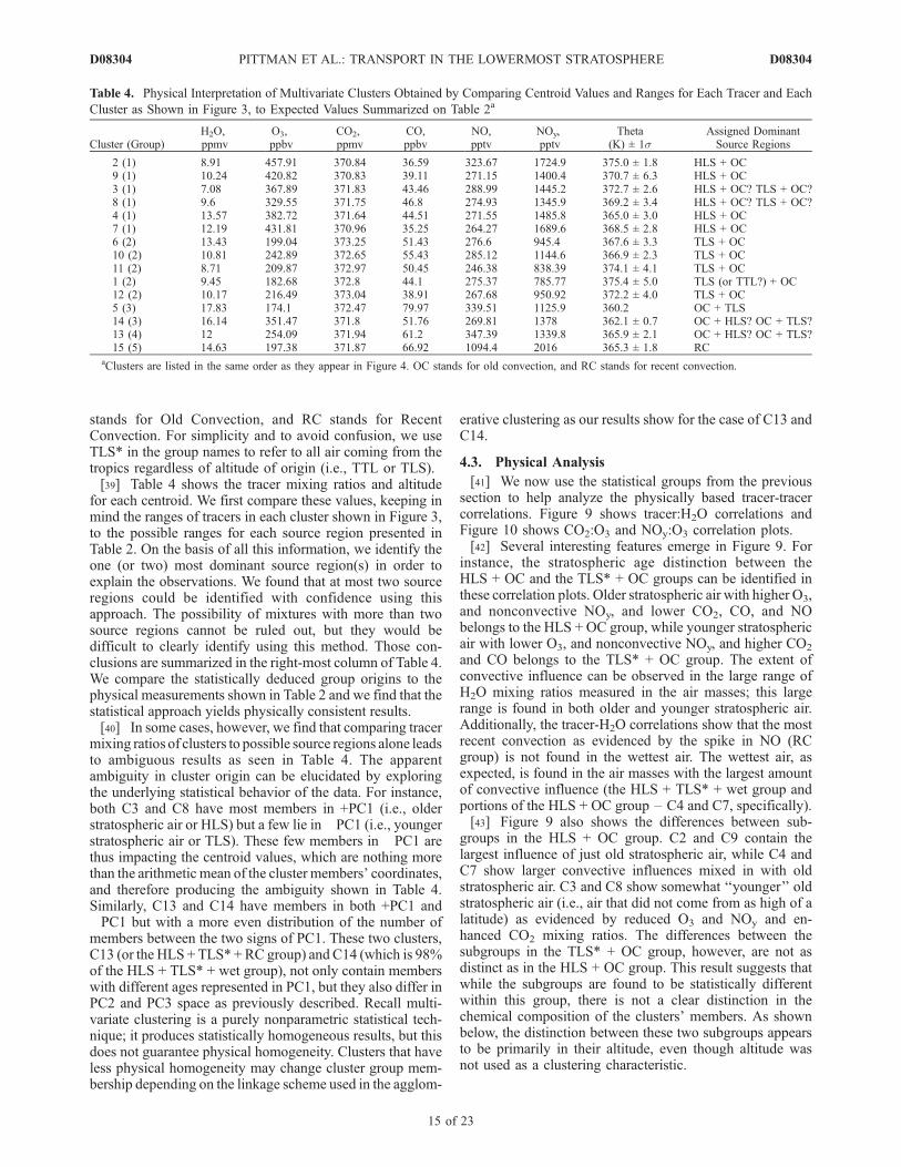
stands for Old Convection, and RC stands for RecentConvection. For simplicity and to avoid confusion, we useTLS* in the group names to refer to all air coming from thetropics regardless of altitude of origin (i.e., TTL or TLS).[39] Table 4 shows the tracer mixing ratios and altitude

for each centroid. We first compare these values, keeping inmind the ranges of tracers in each cluster shown in Figure 3,to the possible ranges for each source region presented inTable 2. On the basis of all this information, we identify theone (or two) most dominant source region(s) in order toexplain the observations. We found that at most two sourceregions could be identified with confidence using thisapproach. The possibility of mixtures with more than twosource regions cannot be ruled out, but they would bedifficult to clearly identify using this method. Those con-clusions are summarized in the right-most column of Table 4.We compare the statistically deduced group origins to thephysical measurements shown in Table 2 and we find that thestatistical approach yields physically consistent results.[40] In some cases, however, we find that comparing tracer

mixing ratios of clusters to possible source regions alone leadsto ambiguous results as seen in Table 4. The apparentambiguity in cluster origin can be elucidated by exploringthe underlying statistical behavior of the data. For instance,both C3 and C8 have most members in +PC1 (i.e., olderstratospheric air or HLS) but a few lie in�PC1 (i.e., youngerstratospheric air or TLS). These few members in �PC1 arethus impacting the centroid values, which are nothing morethan the arithmetic mean of the cluster members’ coordinates,and therefore producing the ambiguity shown in Table 4.Similarly, C13 and C14 have members in both +PC1 and�PC1 but with a more even distribution of the number ofmembers between the two signs of PC1. These two clusters,C13 (or the HLS +TLS* +RC group) and C14 (which is 98%of the HLS + TLS* + wet group), not only contain memberswith different ages represented in PC1, but they also differ inPC2 and PC3 space as previously described. Recall multi-variate clustering is a purely nonparametric statistical tech-nique; it produces statistically homogeneous results, but thisdoes not guarantee physical homogeneity. Clusters that haveless physical homogeneity may change cluster group mem-bership depending on the linkage scheme used in the agglom-

erative clustering as our results show for the case of C13 andC14.

4.3. Physical Analysis

[41] We now use the statistical groups from the previoussection to help analyze the physically based tracer-tracercorrelations. Figure 9 shows tracer:H2O correlations andFigure 10 shows CO2:O3 and NOy:O3 correlation plots.[42] Several interesting features emerge in Figure 9. For

instance, the stratospheric age distinction between theHLS + OC and the TLS* + OC groups can be identified inthese correlation plots. Older stratospheric air with higher O3,and nonconvective NOy, and lower CO2, CO, and NObelongs to the HLS + OC group, while younger stratosphericair with lower O3, and nonconvective NOy, and higher CO2

and CO belongs to the TLS* + OC group. The extent ofconvective influence can be observed in the large range ofH2O mixing ratios measured in the air masses; this largerange is found in both older and younger stratospheric air.Additionally, the tracer-H2O correlations show that the mostrecent convection as evidenced by the spike in NO (RCgroup) is not found in the wettest air. The wettest air, asexpected, is found in the air masses with the largest amountof convective influence (the HLS + TLS* + wet group andportions of the HLS + OC group – C4 and C7, specifically).[43] Figure 9 also shows the differences between sub-

groups in the HLS + OC group. C2 and C9 contain thelargest influence of just old stratospheric air, while C4 andC7 show larger convective influences mixed in with oldstratospheric air. C3 and C8 show somewhat ‘‘younger’’ oldstratospheric air (i.e., air that did not come from as high of alatitude) as evidenced by reduced O3 and NOy and en-hanced CO2 mixing ratios. The differences between thesubgroups in the TLS* + OC group, however, are not asdistinct as in the HLS + OC group. This result suggests thatwhile the subgroups are found to be statistically differentwithin this group, there is not a clear distinction in thechemical composition of the clusters’ members. As shownbelow, the distinction between these two subgroups appearsto be primarily in their altitude, even though altitude wasnot used as a clustering characteristic.

Table 4. Physical Interpretation of Multivariate Clusters Obtained by Comparing Centroid Values and Ranges for Each Tracer and Each

Cluster as Shown in Figure 3, to Expected Values Summarized on Table 2a

Cluster (Group)H2O,ppmv

O3,ppbv

CO2,ppmv

CO,ppbv

NO,pptv

NOy,pptv

Theta(K) ± 1s

Assigned DominantSource Regions

2 (1) 8.91 457.91 370.84 36.59 323.67 1724.9 375.0 ± 1.8 HLS + OC9 (1) 10.24 420.82 370.83 39.11 271.15 1400.4 370.7 ± 6.3 HLS + OC3 (1) 7.08 367.89 371.83 43.46 288.99 1445.2 372.7 ± 2.6 HLS + OC? TLS + OC?8 (1) 9.6 329.55 371.75 46.8 274.93 1345.9 369.2 ± 3.4 HLS + OC? TLS + OC?4 (1) 13.57 382.72 371.64 44.51 271.55 1485.8 365.0 ± 3.0 HLS + OC7 (1) 12.19 431.81 370.96 35.25 264.27 1689.6 368.5 ± 2.8 HLS + OC6 (2) 13.43 199.04 373.25 51.43 276.6 945.4 367.6 ± 3.3 TLS + OC10 (2) 10.81 242.89 372.65 55.43 285.12 1144.6 366.9 ± 2.3 TLS + OC11 (2) 8.71 209.87 372.97 50.45 246.38 838.39 374.1 ± 4.1 TLS + OC1 (2) 9.45 182.68 372.8 44.1 275.37 785.77 375.4 ± 5.0 TLS (or TTL?) + OC12 (2) 10.17 216.49 373.04 38.91 267.68 950.92 372.2 ± 4.0 TLS + OC5 (3) 17.83 174.1 372.47 79.97 339.51 1125.9 360.2 OC + TLS14 (3) 16.14 351.47 371.8 51.76 269.81 1378 362.1 ± 0.7 OC + HLS? OC + TLS?13 (4) 12 254.09 371.94 61.2 347.39 1339.8 365.9 ± 2.1 OC + HLS? OC + TLS?15 (5) 14.63 197.38 371.87 66.92 1094.4 2016 365.3 ± 1.8 RC

aClusters are listed in the same order as they appear in Figure 4. OC stands for old convection, and RC stands for recent convection.


15 of 23

D08304

[44] In addition to tracer:H2O correlations, we examinecorrelations of CO2 and NOy with respect to O3 in Figure 10.Because of their long lifetimes in the stratosphere, theexpected nearly linear and compact correlations are ob-served in this data set to a large extent. The range ofstratospheric age is clearly shown in the progression fromthe HLS + OC group (older stratospheric air characterizedby higher O3, lower CO2, and higher NOy) to the TLS* +OC group (younger stratospheric air characterized by lowerO3, higher CO2, and lower NOy). Of particular interest is thegroup of air masses that depart from the quasi-linearrelation, namely a small fraction of the HLS + TLS* +wet group, and all of the HLS + TLS* + RC and the RCgroups. In these air masses, we find the most recentconvective air as evidenced by higher NOy, which is drivenby high NO, and by lower O3 and CO2, which is consistentwith air of tropospheric character. While these correlationplots are essentially linear, the scatter around the lineindicates that the stratospheric air is not pure, but that it

has been influenced by convection in the past (HLS + OC,TLS* + OC, and HLS + TLS* + wet groups).[45] The air masses that clearly depart from the quasi-

linear relations in Figure 10 are of further interest, becausethey also comprise the group of air masses that reside on adistinct branch away from most of the observations in PCplots shown in Figure 8. In section 4.2, we mentioned thatthe statistical identification of the RC group (i.e., G5) is notentirely consistent with the tracer-tracer plots. On the basisof Figure 8, the RC group is characterized by olderstratospheric air (+PC1) with recent convection (+PC2),but with a smaller than average extent of convectiveinfluence (�PC3). When looking at Figures 9 and 10, wefind that this group has the most recent and not the largestconvective influence as evidenced by the highest NO andhigh H2O; however, O3 mixing ratios clearly indicate thatthis group has younger stratospheric character instead (i.e.,expected negative values for PC1 based on the physicalinterpretation given to eigenvector 1). Recall that thecomputation of each PC consists of taking the product of

Figure 9. Correlations plots of O3, CO2, CO, NO, and NOy with respect to H2O. Color coding is basedon the statistical definitions of cluster groups obtained from agglomerative hierarchical clustering shownin Figure 4. Legend shows cluster numbers followed by (group number). G1 is referred to as HLS + OC,G2 is referred to as TLS* + OC, G3 is referred to as HLS + TLS* + wet, G4 is referred to as HLS +TLS* + RC, and G5 is referred to as RC. See text for details.


16 of 23

D08304

the standardized anomaly of each observation and thecoefficient in the eigenvector for the corresponding tracer(shown in Table 3) and summing up these products, in ourcase a total of six products, one for each tracer used in thisstudy. The most significant tracers in eigenvector 1 are O3,CO2, and NOy. In the case of older stratospheric air, thesethree tracers have all positive contributions to PC1, but inthe case of younger stratospheric air, these three tracers haveall negative contributions instead. Careful examination ofeach term in the products of these three tracers showsnegative anomalies along with a positive weight for O3,negative anomalies along with a negative weight for CO2,and positive anomalies along with a positive weight forNOy. Consequently, O3 has a negative contribution to PC1,but both CO2 and NOy have positive contributions to PC1yielding an overall positive value for PC1 instead of anexpected negative value. In the RC group, NOy is elevatednot because the air mass is of older stratospheric character,but because of the convectively generated NO that drivesthe increase in NOy as shown in Figures 9 and 10. O3 islower than average, because of its tropical origin and notbecause of significant dilution due to the presence ofconvective air, which would be inconsistent with the othertracers. CO2 mixing ratios in this group represent averagevalues and cannot be used to clearly discriminate betweenold and young stratospheric air. Similar results areobtained when carefully examining the members of theHLS + TLS* + RC group that have positive PC1 valuesand share the same branch with the RC group in PC space.This inconsistency between the statistical and physicalanalyses illustrates a shortcoming in the purely statisticaltechnique. While mathematically any combination is possi-ble, an accurate interpretation of the statistical resultsrequires examination of the results in tracer-tracer spaceand use of multiple tracers to properly discriminate differentsource regions.

[46] In addition to looking at tracer mixing ratios, it isalso valuable to explore the temporal evolution of groups ofclusters as a function of altitude. This time series ispresented in Figure 11, grouped by the flights used in thisstudy. Recall that, as discussed above, only flights withmeasurements of all six tracers, in clear air, and in thelowermost stratosphere were considered. Despite the con-straints on data selection, the data we were able to use spanthe entire period of the campaign. Two main dynamicalregimes can be observed in Figure 11 based on the domi-nant presence of the HLS + OC group at the beginning ofthe campaign, and the dominant presence of the TLS* + OCgroup during the middle and the end of the campaign. Theremaining statistical groups are found throughout the cam-paign, and their presence implies that air masses with moreapparent convective influence from both local and nonlocal(recent and old) events were transported to our region ofstudy during the entire campaign.[47] Figure 11 also provides insights into the distinction

between subgroups. For instance, in the HLS + OC group,the C2–C9 couplet is mostly found at higher altitudes whilethe C4–C7 couplet is mostly found at lower altitudes.On the other hand, the C3–C8 couplet is found at allaltitudes. The subgroup in the TLS* + OC group composedof C6, C10, and C11 differs from the C1–C12 couplet inthe same group in that the former is found at lower altitudeswhile the latter is found at higher altitudes. These altitudedifferences emerge as a function of the groupings formed onthe basis of the tracer characteristics.

4.4. Trajectories

[48] The geographical origin and subsequent transport ofthe air ultimately sampled over southern Florida is exam-ined by calculating 10-day backward trajectories with anintegration time step of 30 min using the FABtraj model.The starting location and time for the trajectories varydepending on the group of clusters analyzed as shown in

Figure 10. Correlation plots of CO2 and NOy with respect to O3. Color coding is based on statisticaldefinitions obtained from agglomerative hierarchical clustering shown in Figure 4. Legend shows clusternumbers followed by (group number). G1 is referred to as HLS + OC, G2 is referred to as TLS* + OC,G3 is referred to as HLS + TLS* + wet, G4 is referred to as HLS + TLS* + RC, and G5 is referred to asRC. See text for details.


17 of 23

D08304

Figure 11. Parcels are initially positioned within a volumethat encompasses the latitude, longitude, and altitude of agiven group of clusters sampled by the aircraft on the day ofinterest. This volume extends 55 km in latitude and longi-tude and 5 hPa in altitude past the limits of the aircraftlocation. All trajectories are started at the same time for anygiven day; therefore the presence of different subgroups ofclusters at the same altitude during a given flight cannot beresolved. This constraint, however, is not significant tocompromise the results of this study. All these parcels startin the lowermost stratosphere, and they are separated by5 hPa in the vertical and 55 km in the horizontal.[49] In order to examine the origin of each group,

trajectories are initialized on: 3 July for the HLS + OCgroup, 23 July for the TLS* + OC group, 11 July for theHLS + TLS* + wet group, and 16 July for the HLS +TLS* + RC group. Subgrid convection is not resolved inthis model; therefore trajectory calculations for the RCgroup are not possible, nor are they necessary because thisgroup represents a known local convective event that can be

easily identified in GOES 8 images when the flight track isoverlaid. Plots of the geographical location of the air massesduring the trajectory calculation along with the verticalextent of the trajectories for each of the four groups areshown in Figure 12.[50] Overall, the results of the trajectory calculations are

consistent with the results obtained from tracer compositiongrouped using the statistical techniques. The calculation forthe HLS + OC group shows the old (high-latitude) strato-spheric air component (consistent with high O3), and theanticyclonic flow associated with the North AmericanMonsoon responsible for the equatorward transport of theseair masses as observed in Figure 12a. The calculation for theHLS + TLS* + wet group shows results similar to theHLS + OC group, but it differs in that the air masses do notreach as far north (qualitatively consistent with lower O3

than in the HLS + OC group) and have more of a compo-nent from the subtropical Pacific as observed in Figure 12c.This calculation also shows that air masses are not comingfrom a preferred altitude, but instead from a large range of

Figure 11. Time series of the altitudinal distribution of each statistical group during each flight used inthis study. Legend shows cluster numbers followed by (group number). G1 is referred to as HLS + OC,G2 is referred to as TLS* + OC, G3 is referred to as HLS + TLS* + wet, G4 is referred to as HLS +TLS* + RC, and G5 is referred to as RC. See text for details.


18 of 23

D08304

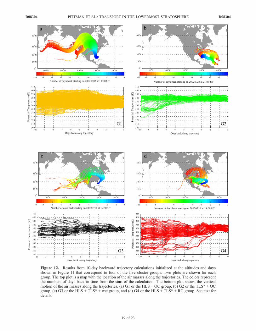
Figure 12. Results from 10-day backward trajectory calculations initialized at the altitudes and daysshown in Figure 11 that correspond to four of the five cluster groups. Two plots are shown for eachgroup. The top plot is a map with the location of the air masses along the trajectories. The colors representthe numbers of days back in time from the start of the calculation. The bottom plot shows the verticalmotion of the air masses along the trajectories. (a) G1 or the HLS + OC group, (b) G2 or the TLS* + OCgroup, (c) G3 or the HLS + TLS* + wet group, and (d) G4 or the HLS + TLS* + RC group. See text fordetails.


19 of 23

D08304

altitudes. Next, the calculation for the HLS + TLS* + RCgroup shows the different source regions previously in-ferred, namely high and tropical latitudes as well as con-vection as observed in Figure 12d. Of particular interest,this group shows a significant influence from the lower andmiddle troposphere over the south central US, and from theboundary layer over the Caribbean, Gulf of Mexico, andFlorida, which are all convective-rich environments duringthis time of the year. These results are consistent with higherNO and CO, and high H2O.[51] We now turn to the TLS* + OC group, which has the

most complex origins. The calculation started on the daychosen to best represent the TLS* + OC group shows thetropical component of air originating from the TTL and/orthe bottom of the lower stratosphere over the Atlantic asobserved in Figure 12b. These results are qualitativelyconsistent with O3 lower than in the HLS + OC group.Members of the TLS* + OC group are also found during theflights of 11 and 16 July, which were chosen to describe theHLS + TLS* + wet and the HLS + TLS* + RC groups,respectively. The trajectories initialized on these two flightdays show some air masses originating from tropical andsubtropical latitudes over the Pacific (11 July case) andmostly over the Atlantic (16 July case) before being trans-ported to southern Florida. Air masses originating over thePacific also travel poleward to higher latitudes beforereaching Florida. The trajectory calculations thus show thatsome members of the TLS* + OC group have a significanttropical and subtropical origin and that the pathways trav-eled from the tropical Pacific or Atlantic are variable duringthe campaign. In addition to examining the horizontalmotion of the air masses in the TLS* + OC group sampledon 23 July, we can also investigate their vertical motion. We

find a significant number of the air masses that remain in themiddle and upper troposphere initially over Florida and laterover the subtropical and tropical Atlantic, a convective-richenvironment, for several days prior to arriving to thelocation of sampling. The rest of the air masses show moreof a quasi-adiabatic flow originating from the TTL and TLSover the tropical Atlantic consistent with lower O3 andhigher CO2 than in the HLS + OC group.[52] Backward trajectories show that the required equa-

torward transport of high-latitude stratospheric air is asso-ciated with the upper level anticyclone that developed overNorth America in July 2002, in agreement with the con-clusions from the work of Richard et al. [2003]. As animportant extension to that previous work, we associate theupper level anticyclone with the North American Monsoon(NAM) that develops over the continent every summer. Thistype of circulation is characterized by a poleward flow of airon the western side and an equatorward flow of air on theeastern side of the monsoon region as shown by Dunkerton[1995]. Because of the distinct chemical composition of thetropical and high-latitude UT/LS, we can use correlationplots of O3 and H2O to confirm the expected impact ofmonsoon circulation on the distribution of these two chem-ical tracers in the UT/LS region.[53] Figure 13 shows the O3:H2O correlation plot using

in situ aircraft data collected over the eastern side of theNAM (i.e., Florida during CRYSTAL-FACE) and overthe western side of the NAM (i.e., California duringSTRAT) in the lowermost stratosphere. In addition totheir location of sampling, these two aircraft campaignsshared similar zonal boundaries (i.e., the jet stream on thenorth side, and the subtropical tropopause on the southside). During the summertime, the subtropical jet stream

Figure 13. H2O:O3 correlation plot using in situ aircraft measurements in the lowermost stratosphereobtained over southern Florida during CRYSTAL-FACE in July 2002 (gray diamonds) and overCalifornia during STRAT in July 1996 (black circles). This plot illustrates the difference in chemicalcomposition between the eastern side (CRYSTAL-FACE) and the western side (STRAT) of the NorthAmerican monsoon.


20 of 23

D08304

is weak because of a significant decrease in the temper-ature gradient between the tropics and the midlatitudes.This condition implies that transport across the tropopausein the subtropics is not inhibited as is the case during thewinter. A climatology study of mixing along the subtrop-ical tropopause as revealed by Rossby Wave Breaking(RWB) events showed that the mixing was indeed morefrequent during the summertime and in particular overregions east of the upper level subtropical high associatedwith monsoon circulation, which together with the weakPV gradients observed during the summer provide favor-able conditions for these mixing events [Postel andHitchman, 1999]. During both campaigns, NCEP-assimilatedhorizontal winds showed the presence of only one jet streamlocated north of 40�N during STRAT, and between 45�Nand 55�N during CRYSTAL-FACE. The observationsshown in Figure 13 are consistent with the expected contrastbetween west and east in the lowermost stratosphere,namely drier air with lower O3 due to poleward transportof tropical air on the west (black circles) versus wetter airdue to transport over continental convective-rich regionsand higher O3 due to equatorward transport of high-latitudestratospheric air on the east (gray diamonds) in agreementwith the results of Gettelman et al. [2004] and Dessler andSherwood [2004]. Therefore summertime transport in thelowermost stratosphere can no longer be thought of asstrictly meridional (i.e., 2-D); the zonal component of theflow also becomes critical at least where influenced bymonsoon circulation consistent with the results of Dunkerton[1995].

4.5. Utility of the Method

[54] The combination of cluster analysis, PCA, tracer-tracer correlations, and trajectory calculations provides anobjective methodology in which a large data set of in situaircraft observations can be reduced to few, natural group-ings that capture the most significant variability of the dataset. In addition to qualitatively describing a data set,quantification of the resulting clusters is desired. We havedeveloped a simple mixing model that uses in situ measure-ments and tracer profiles from selected source regions toquantify the contribution of each of those source regions(E. M. Weinstock et al., Quantifying the impact of the NorthAmerican monsoon and deep midlatitude convection on thesubtropical lowermost stratosphere using in situ measure-ments, submitted to Journal of Geophysical Research,2007, hereinafter referred to as Weinstock et al., submittedmanuscript, 2007). The model calculations are performedon tracer mixing ratios averaged over several flights andusing prescribed convective profiles that best represent thecumulative convective perturbation.[55] The methodology presented in this study can be used

as a data filter for the model. We find consistency in thecomposition of the air mass between the qualitative resultspresented in this study and the quantitative results obtainedfrom the mixing model. For instance, model results for C2,which is a cluster member of the HLS + OC group, show80–90% high-latitude stratospheric air, 10–15% tropicalstratospheric air, and about 3% convective air. Similarly,model results for C6, which is a cluster member of theTLS* + OC group, show 80% tropical stratospheric air,15% high-latitude stratospheric air, and 3% convective air.

Furthermore, the modeled results of the composition ofair masses do not vary significantly within each clustermember and the characterizations of the air mass for dif-ferent cluster members of the same group (e.g., C2 versusC3 in the HLS + OC group) are consistent as well. Thisconsistency between expected fractions of source regionsbased on the objective clustering and the actual valuesobtained from the model constitutes an independent wayof validating the model results.[56] In addition to validating the model results, this

methodology could be used to differentiate convectiveinputs in an objective way and provide a better, moreconstrained fit to the convective fraction. This can beaccomplished by separately analyzing groups of air massesthat have been presumably impacted by convective eventsof different character rather than assigning one convectivesource term to represent multiple convective events.

5. Conclusions

[57] In this study we qualitatively identified the latitudinalorigin and subsequent transport pathways of air sampled inthe subtropical lowermost stratosphere during CRYSTAL-FACE using an objective methodology based on statisticalanalysis, tracer-tracer correlation plots with six differentchemical tracers and backward trajectory calculations. Wefound that the four possible source regions illustrated inFigure 1 were appropriate to describe the transport processesaffecting our region of study.[58] Despite the relatively small size of the data set, the

statistical techniques used and the chosen number of clus-ters proved to be adequate for this task. We are able tostatistically identify and differentiate the presumed domi-nant source regions for the air ultimately sampled duringCRYSTAL-FACE. The majority of the clusters do not haveunique origins, which implies that there is significanthorizontal and/or vertical mixing taking place prior to thearrival of these air masses to our region of sampling. PCAshows that most of the variability in the data set can beexplained primarily by the mean age of air in the strato-sphere, followed by the age of the convective influence, andlast by the extent of the convective influence, which can beassociated with the latitude of convective injection. Whilethe statistical approach is objective, it is important toremember that it is a purely mathematical technique, andan accurate interpretation can only be accomplished byincorporating information based on actual mixing ratiosand tracer-tracer correlations plots as we found to be thecase for the RC group and members of the HLS + TLS* +RC group.[59] We find that different source regions are dominant

during different periods of time. At the beginning of thecampaign, the dominant signature is of high-latitude strato-spheric air while the rest of the campaign is dominated bythe presence of tropical air. On the basis of comparisonswith measurements from previous campaigns, we also findthat the majority of the air masses with tropical signatureoriginate from the TLS rather than the TTL. In some cases,however, air masses have properties of consistent witheither the upper TTL or the lower TLS. Because thisboundary is not very distinct in terms of tracer mixing


21 of 23

D08304

ratios, we cannot exclude the possibility of TTL air presentin our region of study.[60] Very moist air is ubiquitously present during the

entire campaign and throughout the subtropical lowermoststratosphere. Enhancements in H2O were associated witha local convective event in one case only (21 July) as alsoevidenced by the significant spike in NO. The rest of thetime, air masses with up to 22 ppmv of H2O (clear convec-tive signature) contained less than 400 pptv of NO, whichsuggests nonlocal convective air that came from the tropicsor that was injected in the UT/LS region at higher latitudesand it was subsequently transported over the course of a fewdays to a week into our region of sampling.[61] Backward trajectory calculations confirmed the lati-

tudinal origin of the air masses sampled during the cam-paign. The trajectories also showed that monsooncirculation plays a critical role in the distribution of keyradiative species such as H2O and O3 in the UT/LS.Therefore the canonical view of a purely meridional (i.e.,2-D) large-scale circulation linking the stratosphere and thetroposphere cannot be treated as universal. Over monsoonregions, both meridional and zonal transport pathways needto be considered as well as the longitude of the meridionaltransport, which can be either poleward or equatorward.[62] Last, the methodology presented in this study was

used to compare results with a mixing that provides thefractional contribution of each source region (Weinstock etal., submitted manuscript, 2007). We found consistentresults between the qualitatively identified source regionsobtained in this study and the model-derived contribution ofeach source region.

[63] Acknowledgments. We are very grateful to the WB-57 flightand ground crews as well as the CRYSTAL-FACE mission planners fortheir hard work in making this campaign possible. We thank the NOAAClimate Monitoring and Diagnostics Laboratory for providing surfacemeasurements. We thank D. Boccippio for providing insightful commentson the statistical analysis presented in this work. We are also grateful toP. Robertson, T. Miller, and the anonymous reviewers for their helpfulcomments and suggestions. J. V. Pittman acknowledges the NASA EarthSystem Science Graduate Student Fellowship (grant NGT5-3040) for theirsupport during the course of this research project. This work was funded inpart by the NASA Upper Atmospheric Research Program. Work performedby M.J.M. at the Jet Propulsion Laboratory, California Institute of Tech-nology, was done under contract with NASA.

ReferencesBoccippio, D. J., W. A. Petersen, and D. J. Cecil (2005), The tropicalconvective spectrum: Part I: Archetypal vertical structures, J. Clim., 18,2744–2769.

Boering, K. A., S. C. Wofsy, B. C. Daube, H. R. Schneider,M. Loewenstein, J. R. Podolske, and T. J. Conway (1996), Stratosphericmean ages and transport rates from observations of carbon dioxide andnitrous oxide, Science, 274, 1340–1343.

Brasseur, G., and S. Solomon (1986), Aeronomy of the Middle Atmosphere:Chemistry and Physics of the Stratosphere and Mesosphere, Dordrecht,Boston, Mass.

Brewer, A. W. (1949), Evidence for a world circulation provided by mea-surements of helium and water vapor in the stratosphere, Q. J. Roy.Meteorol. Soc., 75, 351–363.

Chen, P. (1995), Isentropic cross-tropopause mass-exchange in the extra-tropics, J. Geophys. Res., 100, 16,661–16,673.

Cooper, O., et al. (2004a), A case study of trans-Pacific warm conveyor belttransport: The influence of merging airstreams on trace gas import toNorth America, J. Geophys. Res., 109, D23S08, doi:10.1029/2003JD003624.

Cooper, O. R., et al. (2004b), On the life-cycle of a stratospheric intrusionand its dispersion into polluted warm conveyor belts, J. Geophys. Res.,109, D23S09, doi:10.1029/2003JD004006.

Daube, B. C. J., K. A. Boering, A. E. Andrews, and S. C. Wofsy (2002), Ahigh-precision fast-response airborne CO2 analyzer for in situ samplingfrom the surface to the middle stratosphere, J. Atmos. Ocean Technol., 19,1532–1543.

Denning, R. F., S. L. Guidero, G. S. Parks, and B. L. Gary (1989), Instru-ment description of the airborne microwave temperature profiler, J. Geo-phys. Res., 94, 16,757–16,765.

Dessler, A. E., and S. C. Sherwood (2004), The effect of convection on thesummertime extratropical lower stratosphere, J. Geophys. Res., 109,D23301, doi:10.1029/2004JD005209.

Dessler, A. E., E. M. Weinstock, E. J. Hintsa, J. G. Anderson, C. R.Webster, R. D. May, J. W. Elkins, and G. S. Dutton (1994), An examina-tion of the total hydrogen budget of the lower stratosphere, Geophys. Res.Lett., 21, 2563–2566.

Dessler, A. E., E. J. Hintsa, E. M. Weinstock, J. G. Anderson, and K. R.Chan (1995), Mechanisms controlling water vapor in the lower strato-sphere: A tale of two stratospheres, J. Geophys. Res., 100, 23,167–23,172.

Dethof, A., A. O’Neill, and J. Slingo (2000), Quantification of the isen-tropic mass transport across the dynamical tropopause, J. Geophys. Res.,105, 12,279–12,293.

Dobson, G. M. B. (1956), Origin and distribution of the polyatomicmolecules in the atmosphere, Proc. R. Soc. London, Ser. A, 236,187–193.

Dunkerton, T. J. (1995), Evidence of meridional motion in the summerlower stratosphere adjacent to monsoon regions, J. Geophys. Res., 100,16,675–16,688.

Fahey, D. W., K. K. Kelly, D. M. Murphy, G. V. Ferry, M. Loewenstein,K. R. Chan, L. R. Poole, and J. C. Wilson (1989), In situ measurementsof total reactive nitrogen, total water, and aerosol in a polar stratosphericcloud in the Antarctic, J. Geophys. Res., 94, 11,299–11,315.

Fahey, D. W., et al. (1996), In situ observations of NOy, O3, and theNOy/O3 ratio in the lower stratosphere, Geophys. Res. Lett., 23, 1653–1656.

Gettelman, A., and P. M. D. Forster (2002), A climatology of the tropicaltropopause layer, J. Meteorol. Soc. Jpn., 80, 911–924.

Gettelman, A., D. E. Kinnison, T. J. Dunkerton, and G. P. Brasseur (2004),Impact of monsoon circulations on the upper troposphere and lowerstratosphere, J. Geophys. Res., 109, D22101, doi:10.1029/2004JD004878.

Hargrove, W. W., and F. M. Hoffman (2004), The potential of multivariatequantitative methods for delineation and visualization of ecoregions,Environ. Manage., 34, S39–S60.

Hintsa, E. J., et al. (1998), Troposphere-to-stratosphere transport in thelowermost stratosphere from measurements of H2O, CO2, N2O and O3,Geophys. Res. Lett., 25, 2655–2658.

Hoffman, F. M., W. W. Hargrove, D. J. Erickson III, and R. J. Oglesby(2005), Using clustered climate regimes to analyze and compare predic-tions from fully coupled general circulation models, Earth Interact., 9,EI110, doi:10.1175/EI110.1.

Holton, J. R., P. H. Haynes, M. E. McIntyre, A. R. Douglass, R. B. Rood,and L. Pfister (1995), Stratosphere-troposphere exchange, Rev. Geophys,33, 403–439.

Hoor, P., H. Fischer, L. Lange, J. Lelieveld, and D. Brunner (2002), Sea-sonal variations of a mixing layer in the lowermost stratosphere as iden-tified by the CO-O3 correlation from in situ measurements, J. Geophys.Res., 107(D5), 4044, doi:10.1029/2000JD000289.

Hoskins, B. J. (1991), Towards a PV-Theta view of the general circulation,Tellus, Ser. A, 43, 27–35.

Hurst, D. F., et al. (1999), Closure of the total hydrogen budget of the northernextratropical lower stratosphere, J. Geophys. Res., 104, 8181–8200.

Jensen, E., D. Starr, and O. B. Toon (2004), Mission investigates tropicalcirrus clouds, Eos Trans. AGU, 85, 45.

Jost, H. J., et al. (2004), In situ observations of mid-latitude forest fireplumes deep in the stratosphere, Geophys. Res. Lett., 31, L11101,doi:10.1029/2003GL019253.

Loewenstein, M., H. Jost, J. Grose, J. Eilers, D. Lynch, S. Jensen, andJ. Marmie (2002), Argus: A new instrument for the measurement ofthe stratospheric dynamical tracers, N2O and CH4, Spectrochim. ActaA, 58, 2329–2345.

Mote, P. W., K. H. Rosenlof, M. E. McIntyre, E. S. Carr, J. C. Gille, J. R.Holton, J. S. Kinnersley, H. C. Pumphrey, J. M. Russell, and J. W. Waters(1996), An atmospheric tape recorder: The imprint of tropical tropopausetemperatures on stratospheric water vapor, J. Geophys. Res., 101, 3989–4006.

Murphy, D. M., D. W. Fahey, M. H. Proffitt, S. C. Liu, K. R. Chan, C. S.Eubank, S. R. Kawa, and K. K. Kelly (1993), Reactive nitrogen and itscorrelation with ozone in the lower stratosphere and upper troposphere,J. Geophys. Res., 98, 8751–8773.

Plumb, R. A. (2002), Stratospheric transport, J. Meteorol. Soc. Jpn., 80,793–809.


22 of 23

D08304

Plumb, R. A., and M. K. W. Ko (1992), Interrelationships between mixingratios of long lived stratospheric constituents, J. Geophys. Res., 97,10,145–10,156.

Postel, G. A., and M. H. Hitchman (1999), A climatology of Rossby wavebreaking along the subtropical tropopause, J. Atmos. Sci., 56, 359–373.

Poulida, O., R. R. Dickerson, and A. Heymsfield (1996), Stratosphere-troposphere exchange in a midlatitude mesoscale convective complex,J. Geophys. Res., 101, 6823–6836.

Prados, A. I., G. E. Nedoluha, R. M. Bevilacqua, D. R. Allen, K. W.Hoppel, and A. Marenco (2003), POAM III ozone in the upper tropo-sphere and lowermost stratosphere: Seasonal variability and comparisonsto aircraft observations, J. Geophys. Res., 108(D7), 4218, doi:10.1029/2002JD002819.

Proffitt, M. H., and R. J. McLaughlin (1983), Fast-response dual-beam UV-absorption ozone photometer suitable for use on stratospheric balloons,Rev. Sci. Instrum., 54, 1719–1728.

Ray, E. A., et al. (2004), Evidence of the effect of summertime midlatitudeconvection on the subtropical lowermost stratosphere from CRYSTAL-FACE tracer measurements, J. Geophys. Res., 109, D18304, doi:10.1029/2004JD004655.

Richard, E. C., K. C. Aikin, E. A. Ray, K. H. Rosenlof, T. L.Thompson, A. Weinheimer, D. Montzka, D. Knapp, B. Ridley, andA. Gettelman (2003), Large-scale equatorward transport of ozone inthe subtropical lower stratosphere, J. Geophys. Res., 108(D23), 4714,doi:10.1029/2003JD003884.

Ridley, B. A., J. G. Walega, J. E. Dye, and F. E. Grahek (1994), Distribu-tions of NO, NOx, NOy, and O3 to 12-km altitude during the summermonsoon season over New Mexico, J. Geophys. Res., 99, 25,519–25,534.

Ridley, B. A., J. E. Dye, J. G. Walega, J. Zheng, F. E. Grahek, and W. Rison(1996), On the production of active nitrogen by thunderstorms over NewMexico, J. Geophys. Res., 101, 20,985–21,005.

Ridley, B. A., et al. (2004), Florida thunderstorms: A faucet of reactivenitrogen to the upper troposphere, J. Geophys. Res., 109, D17305,doi:10.1029/2004JD004769.

Shah, K. P., and D. Rind (1998), Comparing upper tropospheric and lowerstratospheric temperatures: Microwave sounding unit, radiosonde,COSPAR International Reference Atmosphere, and National Centersfor Environmental Prediction/National Center for Atmospheric Researchreanalysis monthly mean climatologies, J. Geophys. Res., 103, 31,569–31,592.

Stohl, A., et al. (2003), Stratosphere-troposphere exchange: A review, andwhat we have learned from STACCATO, J. Geophys. Res., 108(D12),8516, doi:10.1029/2002JD002490.

Strahan, S. E. (1999), Climatologies of lower stratospheric NOy and O3 andcorrelations with N2O based on in situ observations, J. Geophys. Res.,104, 30,463–30,480.

Strahan, S. E., A. R. Douglass, J. E. Nielsen, and K. A. Boering (1998), TheCO2 seasonal cycle as a tracer of transport, J. Geophys. Res., 103,13,729–13,742.

Thompson, T. L. and K. H. Rosenlof (2003), Accuracy and precision of theNOAA Aeronomy Laboratory pressure temperature instrument on the

NASA WB-57F, paper presented at CRYSTAL-FACE Science TeamMeeting, Natl. Aeronaut. Space Admin., Salt Lake City, Utah.

Vaughan, G., and C. Timmis (1998), Transport of near-tropopause air intothe lower midlatitude stratosphere, Q J. Roy. Meteorol. Soc., 124, 1559–1578.

Webster, C. R., R. D. May, C. A. Trimble, R. G. Chave, and J. Kendall(1994), Aircraft (ER-2) Laser Infrared Absorption Spectrometer (ALIAS)for in-situ stratospheric measurements of HCl, N2O, CH4, NO2, andHNO3, Appl. Opt., 33, 454–472.

Weinstock, E. M., C. M. Schiller, and J. G. Anderson (1986), In situ strato-spheric ozone measurements by long path UVabsorption–Developmentsand interpretation, J. Geophys. Res., 91, 5237–5248.

Weinstock, E. M., E. J. Hintsa, A. E. Dessler, J. F. Oliver, N. L. Hazen, J. N.Demusz, N. T. Allen, L. B. Lapson, and J. G. Anderson (1994), New fast-response photofragment fluorescence hygrometer for use on the NASAER-2 and the Perseus remotely piloted aircraft, Rev. Sci. Instrum., 65,3544–3554.

Weinstock, E. M., E. J. Hintsa, D. B. Kirk-Davidoff, J. G. Anderson, A. E.Andrews, R. L. Herman, C. R. Webster, M. Loewenstein, J. R. Podolske,and T. P. Bui (2001), Constraints on the seasonal cycle of stratosphericwater vapor using in situ measurements from the ER-2 and a CO photo-chemical clock, J. Geophys. Res., 106, 22,707–22,724.

Wilks, D. S. (2006), Statistical Methods in the Atmospheric Sciences, Else-vier, New York.

��J. G. Anderson, B. C. Daube, D. S. Sayres, J. B. Smith, E. M. Weinstock,

and S. C. Wofsy, Department of Earth and Planetary Sciences, HarvardUniversity, Cambridge, MA 02138, USA.O. R. Cooper, Cooperative Institute for Research in Environmental

Sciences, University of Colorado, Boulder, CO 80309, USA.C. Gerbig, Max Planck Institute for Biogeochemistry, D-07745 Jena,

Germany.W. W. Hargrove and F. M. Hoffman, Oak Ridge National Laboratory,

Oak Ridge, TN 37831, USA.H.-J. Jost, NovaWave Technologies, Redwood City, CA 94065, USA.M. Loewenstein, NASA Ames Research Center, Moffett Field, CA

94035, USA.J. P. Lopez, Bay Area Environmental Research Institute, Sonoma, CA

95476, USA.M. J. Mahoney, Jet Propulsion Laboratory, California Institute of

Technology, Pasadena, CA 91109, USA.R. J. Oglesby, Department of Geosciences, University of Nebraska,

Lincoln, NE 68588, USA.J. V. Pittman, NASA Marshall Space Flight Center, Huntsville, AL

35805, USA. ([email protected])E. C. Richard and T. L. Thompson, Earth System Research Laboratory,

NOAA, Boulder, CO 80305, USA.B. A. Ridley, and A. J. Weinheimer, Atmospheric Chemistry Division,

National Center for Atmospheric Research, Boulder, CO 80305, USA.I. Xueref, Laboratoire des Sciences du Climat et de l’Environment,

Commissariat l’Energie Atomique, F-91191 Gif-Sur-Yvette Cedex, France.


23 of 23

D08304

Transport in the subtropical lowermost stratosphere during the Cirrus Regional Study of Tropical Anvils and Cirrus Layers–Florida Area Cirrus Experiment

Documents