Transmitters and Receivers Dr Costas Constantinou School of Electronic, Electrical & Computer Engineering University of Birmingham W:

Transmitters and Receivers

Dr Costas ConstantinouSchool of Electronic, Electrical & Computer Engineering

University of BirminghamW: www.eee.bham.ac.uk/ConstantinouCC/

E: [email protected]

The Communication Process

• Every communication system has 3 basic elements (in blue):– Transmitter– Channel– Receiver

• Information

• Source

• Transmitt

er

• Channel

• Information

• Sink

• Receiver

• Message

• signal

• Estimated message

• signal• Trans

mitted signal

• Received signal

2

3

The Source

OSI reference model

data

data

data

data

data

dataAPSTN

APST

APS

AP

A

dataAPSTND

analogue

Note accumulation of control data at each level.

For small packets control information can be much more than the data itself

4

The source

• The message signal can be either analogue or digital

• The transmitted signal is always analogue – why?– Simultaneous communications: Multiplexing– Bandwidth limiting

5

Multiplexing

• No multiplexing = one physical transmission medium per user!

• Sharing transmission medium is central to communications

6

Why Multiplex

• Mobile phone has voice plus many control channels simultaneously

• Optical fibre very high capacity for many simultaneous channels

• Putting many telephone calls over one cable

Key feature of digital waveforms – limit bandwidth

0

0.2

0.4

0.6

0.8

1

1.2

1.4

S1

0

0.2

0.4

0.6

0.8

1

1.2

1.4

frequency

frequency

A

t

F = 1/t

time

A

time

Pass through raised cosine filter to remove frequency side-lobes

Choose bit rate to match channel bandwidth

7

8

Key feature of digital waveforms – limit bandwidth

All standardized common TTL circuits operate with a 5 V power supply. TTL signal is defined as:– "low" when between 0V and 0.8V with respect to the ground – "high" when between 2.2V and 5V

CMOS works with a wider range of power supply voltage –usually anywhere from 3 to 15V

Current ~ 1 mA or lower

A

time

9

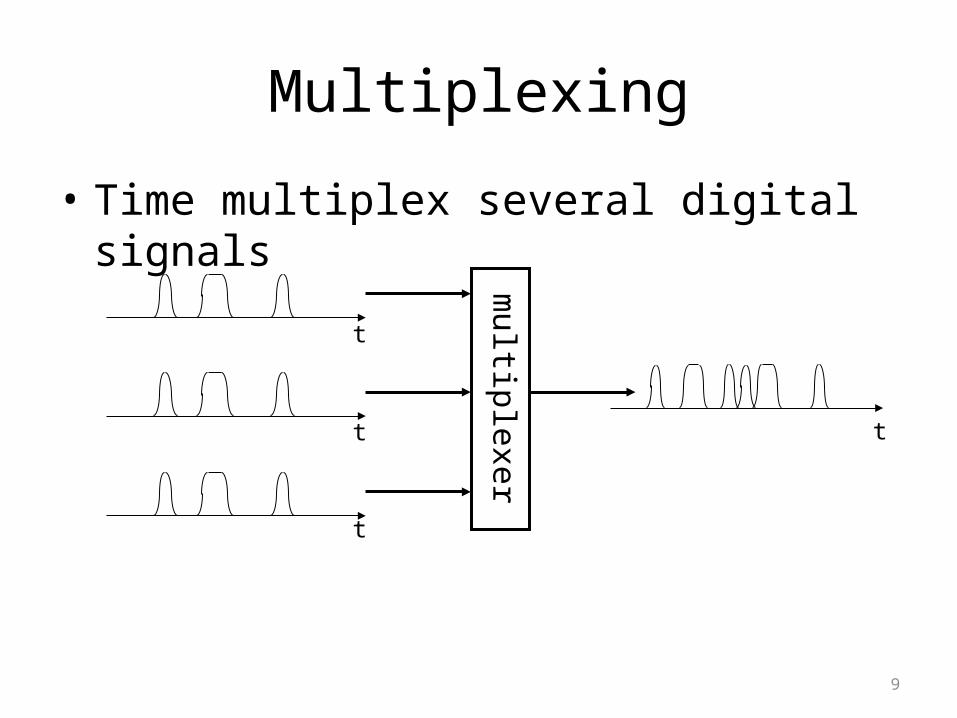
Multiplexing

• Time multiplex several digital signals

multiplexer

t

t

t

t

10

The Transmitter• Transmitter power must be sufficient to achieve

adequate signal strength at the receiver• Received signal must be higher than noise to be

intelligible

power

txtx

distance

power

distance

receiverreceiver

noise

noise

txtx receiverreceiver

signal tonoise ratio

signal tonoise ratio

good ! bad !

11

Transmitter power

• Need amplification to increase transmitted power to overcome loss in the channel

• Power level depends on channel loss• Channel loss depends on distance. Typical order of

magnitude figures– telephone cable ~ 20 dB– optical fibre ~ 30 dB– wireless channel ~ 80 dB

12

Transmitter bandwidth

• We want to get as many user channels into the transmitter bandwidth as possible

• Baseband voice bandwidth ~ 3kHz• Percentage of user channel to centre frequency

telephone 10 - 13 kHz ~ 26 %multiplexed telephone 1 – 1.003 MHz ~ 0.29 %mobile phone 850 – 850.003 MHz ~ 3 x 10-6 %optical fibre 300 THz – 300 THz + 3 kHz ~ 10-11 %

• Conclusion – upconvert to higher frequencies

13

Other reasons to upconvert

• Fibre optic– cannot get electrical signals down an insulating

glass fibre

• Wireless– for efficient operation antennas => λ/2

at 3 kHz λ = c/f = 3 x 108/3 x 103 = 100 kmat 3 GHz λ = 0.1 m

14

Upconverters

• Use a mixer– Assume input signal is digital 1,0,1,0,1…..

– Apply carrier signal to other port,

– Output is product (mixer is multiplier)

Vc

Vo

t

cosc cV tfreq

tnn

AVs 0cos

2

ttnn

AV co

coscos

20

15

Upconverters

• Simplify using trigonometric expansion

gives

• Mixer produces difference and sum frequencies of all components in input waveform

Vc

Vo

t

1 1cos cos cos cos

2 2A B A B A B

0 0

1 2cos cos

2o c c

AV n t n t

n

16

signal f1

carrier f2

sum (f2 + f1) and

difference (f2 - f1)

Assume input is digitised speech

signal = 0 - 3 kHz

carrier = 6 kHz

sum = 6 - 9 kHz

difference = 3 - 6 kHz

freq

freq

freq

Upconverters

17

To reduce bandwidth remove sum frequency

filter performance

0

0.1

0.2

0.3

0.4

0.5

0.6

0.7

0.8

0.9

1

1 2 3 4 5 6 7 8 9 10 11 12 13 14

frequency, kHz

mixer filter

0-3kHz

6kHz

6-9kHz

3-6kHz

3-6kHzfreq

Upconverters

18

• Non-linear devices such as diode have a current/voltage relationship which includes a square law characteristic

• 2nd term is the product that we want for upconversion

I

V

Upconverters – the mixer circuit

2

220

2 2 20 0

cos cos

cos 2cos cos cos

c

c c

I kV

kA t t

kA t t t t

19

• Using

gives

• We need to filter the DC term as well as the much higher frequency 2ωc and much lower frequency 2ωo

20

cos2 cos21 2cos cos

2 2c o

c

t tI kA t t

Upconverters – the mixer circuit

2 1 cos2cos

2

AA

20

The Transmitter – so far

Note – can change output frequency by tuning ωc

ωc

mul

tiple

xer

sourcesource

source

tfreq local

oscillator

amplifier 1 amplifier 2

freq

freq

t

t

21

ωcm

ultip

lexe

r

sourcesource

source

amplifier 1 amplifier 2

Amplifier 1: needed to get digital signal up to level needed by mixer circuitAmplifier 2: needed to get mixer output up to level required by channel

e.g. mobile phone output power 1 watt max. mixer output – 1 mA at 5 V amp. output - 100 mA at 5 V

The Transmitter – so far

22

The Channel

• Channel problems– A – channel attenuates signal (attenuation can be variable)

– B – channel is dispersive (speed varies with frequency)

Cable A – moderate, B – limits upper frequency and data rate

Fibre A – low, B – limits upper frequency and data rate

WirelessA – very high and variable, B – bad in urban and indoors

TxRx

Cable or fibre

TxRx

wireless

23

Pulse or packet• waveform

• spectrum

frequency

time

Dispersion

• Signals are usually many frequencies added together

24

• Wave groups– Ripples in pond from a dropped stone– Pulse on a transmission line

Non dispersive – All frequencies travel at same speed. Packet shape not changed.

Dispersive –Frequencies travel at different speeds. Packet shape widens.

Dispersion

25

Channel Variability

• The effect of noise– Decision making in a 2 level signal

time

0 1 0 1

1

0

26

Channel Variability

• Decision making in a 4 level signal

time

0 21 3

3

0

smaller amounts of noise are more significant as number of levels increases

2

1

27

Channel Variability

• Can we find a waveform that is less affected by amplitude noise?

• Fundamental properties of a signal– Amplitude– Frequency– Phase

• Amplitude modulation used so far

28

• Amplitude modulation

• Frequency or phase modulation

Possible Modulation Schemes

29

Noise mainly in peaks

Frequency/Phase Modulation

• To remove amplitude noise from frequency or phase modulation– Amplify

Clip– count zero crossings to determine instantaneous frequency

• Called a limiter – see Signal Processing module

30

Frequency Modulator Concept

Amplifier

Feedback

- becomes oscillator

(C determines frequency)

Vary capacitance using varactor diode

(frequency depends on signal voltage)

Vs

f(Vs)

31

Final Transmitter?

mul

tiple

xer

sourcesource

source

ωc

modulator

32

Final Transmitter?

• Output waveform spectrum must meet template laid down by international agreement (ITU), especially for wireless systems

• Typical template (GSM)890 960

Freq (MHz)

Power (dBm)

+30

-70

Allowed out of band radiation

channel

Conclusion – must use band pass filter at output

33

Final transmitter

mul

tiple

xer

sourcesource

source

ωc

modulator

34

The Receiver

• Assume amplitude modulation of digital signal

• Single modulated pulse looks like

freq

time

35

• Received signal

• Rectify pulse to remove lower half

• Low pass filter to get envelope

• Amplify

36

The detector

The first radio sets used a rectifier and a tuned circuit.

The rectifier was made from a wire touching a piece of crystal material, called a cats whisker

37

The detector• Advantages

– simple construction– suitable for cable systems– optical fibres use laser diode as transmitter and detector diode as receiver

• Disadvantages– not very sensitive to small signals– cannot be used in wireless systems

• Wireless systems– low signal strength – use low noise amplifier (LNA)– external noise – use filter

TxRx

external noise

38

External Noise Power

power

Freq (MHz)

10 100 1000

Filter for FM broadcast band

Filter for GSM mobile phones

Note – filters cover whole band

– channel filters discussed later

39

Improved receiver

• The loss of the BPF and the detection process in the rectifier both contribute noise.

• Low noise amplifier (LNA) also adds noise, but at lower level.

• Gain of the LNA should be high enough so that LNA noise dominates.

• More details of noise calculations in the link budget lectures.

low noise amp

band-pass filter

40

Thermal Noise Power

• Since spectrum is flat with frequency (white noise)– then noise power must be proportional to bandwidth

Pn = k T B Watts

– wherePn = available noise power, in Watts

– k = Boltzmann’s constant = 1.38 x 10-23 Joule/Kelvin

– T = absolute temperature of noise source, in Kelvin

– B = bandwidth, in Hz

41

• For a bandwidth of 1 MHz the available noise power from a source at temperature 300 K is

Pn = 1.38 x 10-23 x 300 x 1 x 106 ~ 4 x 10-15 W

• Compare this with a signal power generated by a 1.0µV source driving a 50 Ohm load which results in an available signal power of

Ps = (1.0 x 10-6)2 / 4 x 50 = 5 x 10-15 W

• If the noise is comparable to the signal then subsequent amplification will not improve matters

Thermal Noise Power

42

Improved Receiver - A

Filter design

Vout/Vin

freq

f0

Δf

Quality factor = f0 / Δf

Max. Q factor for typical filter is few thousand

low noise amp

band-pass filter

43

Filters• For GSM mobile phone band

– complete band = 890 – 960 MHz = 70 MHz

– channel bandwidth = 25 kHz

• Q factor needed– complete band = 925 / 70 = 11.8

– channel bandwidth = 925x106 / 25x103 = 33,000

• Conclusion– can filter whole band, but not user channel

– but downconversion may help……

Bandpass filter

890 freq (MHz) 960

band

channelTx Rx

44

Improved Receiver - B

• Downconverter is same as upconverter

fout = fc – fs = fintermediate = IF

low noise amp band filter

ωc

downconverter detector

45

Improved Receiver - B

• Additions– normal to include low-pass filter as part of mixer

– as LNA may have only low gain, put in another amplifier

– put in channel filter

– IF signal retains phase/frequency as well as amplitude information

– represent detector as block which could also detect PM/AM

low noise amp

band filter

ωc

detector

channel filter

IF amp

downconverter

46

Improved Receiver - C

• IF amp may have gain ~ 40 dB

• Channel filter (assume IF = 100 MHz– Q factor = 100x 106 / 25x103 = 4000

– realised with a surface acoustic wave filter

low noise amp

band filter

ωc

detector

channel filter

IF amp

downconverter

47

Improved Receiver - C

• Can tune local oscillator to choose receive frequency

– fIF = fc – fs

• IF is fixed and fc is changed to select wanted channel

• Easier to tune oscillator than make tuned filter

• Example

– fIF = 100 MHz, fc = 998, fs = 898

– fIF = 100 MHz, fc = 1040, fs = 940890 freq (MHz) 960

band

channelTx Rx

low noise amp

band filter

ωc

detector

channel filter

IF amp

downconverter

48

Improved receiver - C

• Example

fIF = 100 MHz, fc = 1040, fs = 940

• Problem

fIF = 100 MHz, fc = 1040, fimage = 1140

signal at fs + 2IF will also go through mixer

must filter out ‘image signal’ with band filter/image reject mixer

IF fs fc fimage

low noise amp

band filter

ωc

detector

channel filter

IF amp

downconverter

49

Transceiver

low noise ampband filter

ωc

detector

channel filter

IF amp

multiplexed source

modulator

o/p

band filter high power amp

local oscillator

antenna

diplexer

50

The Future?Direct Up/Downconversion and Software Defined Radio

• Intermediate frequency is zero (baseband)

• Channel filtering and demodulation done by digital processing.

• Processing can be changed to make radio work with any standard, or even download software for new standards over the air!

ωc

processora/d converter

51

What next?

• Attempt the tutorial sheet on transmitters and receivers

• Next lecture on antennas