HAL Id: tel-01080577 https://pastel.archives-ouvertes.fr/tel-01080577 Submitted on 5 Nov 2014 HAL is a multi-disciplinary open access archive for the deposit and dissemination of sci- entific research documents, whether they are pub- lished or not. The documents may come from teaching and research institutions in France or abroad, or from public or private research centers. L’archive ouverte pluridisciplinaire HAL, est destinée au dépôt et à la diffusion de documents scientifiques de niveau recherche, publiés ou non, émanant des établissements d’enseignement et de recherche français ou étrangers, des laboratoires publics ou privés. Transmitter and receiver design for multi-antenna interfering systems Francesco Negro To cite this version: Francesco Negro. Transmitter and receiver design for multi-antenna interfering systems. Other. Télécom ParisTech, 2012. English. NNT: 2012ENST0049. tel-01080577

Welcome message from author
This document is posted to help you gain knowledge. Please leave a comment to let me know what you think about it! Share it to your friends and learn new things together.
Transcript

HAL Id: tel-01080577https://pastel.archives-ouvertes.fr/tel-01080577
Submitted on 5 Nov 2014
HAL is a multi-disciplinary open accessarchive for the deposit and dissemination of sci-entific research documents, whether they are pub-lished or not. The documents may come fromteaching and research institutions in France orabroad, or from public or private research centers.
L’archive ouverte pluridisciplinaire HAL, estdestinée au dépôt et à la diffusion de documentsscientifiques de niveau recherche, publiés ou non,émanant des établissements d’enseignement et derecherche français ou étrangers, des laboratoirespublics ou privés.
Transmitter and receiver design for multi-antennainterfering systems
Francesco Negro
To cite this version:Francesco Negro. Transmitter and receiver design for multi-antenna interfering systems. Other.Télécom ParisTech, 2012. English. �NNT : 2012ENST0049�. �tel-01080577�

2012-ENST-049
Doctorat ParisTech
T H È S E
pour obtenir le grade de docteur délivré par
TELECOM ParisTech
Spécialité : « Electronique et Communications »
présentée et soutenue publiquement par
Francesco NEGROle 26 Septembre 2012
Conception de Transmetteurs et de Rècepteurs pour desSystèmes à Interfèrences avec Antennes Multiples
Directeur de thèse : Dirk T.M. SLOCK
JuryM. Eduard Jorswieck, Professeur, TU Dresden, Germany Rapporteur
M. Maxime Guillaud, Docteur, TU Wien, Austria Rapporteur
M. David Gesbert, Professeur, EURECOM, France Examinateur
M. Mérouane Debbah, Professeur, Supelec Paris, France Examinateur
M. Luc Deneire, Professeur, University of Nice, France Examinateur
M. Irfan Ghauri, Docteur, Intel Mobile Communications, France Invité
TELECOM ParisTechécole de l’Institut Télécom - membre de ParisTech


2012-ENST-049
Dissertation ParisTech
THESIS
In partial fulfillment of the requirements for the degree of
doctor of philosophy from
TELECOM ParisTech
Specialization : « Electronics and Communications »
presented and publicly defended by
Francesco NEGRO
the 26th of September 2012
Transmitter and Receiver Design for Multi-Antenna Interfering
Systems
Thesis Supervisor : Dirk T.M. SLOCK
Committee
M. Eduard Jorswieck, Professor, TU Dresden, Germany Reviewer
M. Maxime Guillaud, Doctor, TU Wien, Austria Reviewer
M. David Gesbert, Professor, EURECOM, France Examiner
M. Mérouane Debbah, Professor, Supelec Paris, France Examiner
M. Luc Deneire, Professor, University of Nice, France Examiner
M. Irfan Ghauri, Doctor, Intel Mobile Communications, France Invitee
TELECOM ParisTech
école de l’Institut Télécom - membre de ParisTech


Abstract
In modern wireless communication systems, the per-user data rate demand is con-
stantly growing. In addition the rapid evolution of mobile services accentuates this
evolution. To sustain the heavy user data rate demand network operators try to
deploy cellular system with more cells and applying more efficient spectrum reuse
techniques. One possible solution to increase system throughput is to get the user
closer to the transmitting base station and hence deploy very dense network infras-
tructure. A possible way to reduce the costs of deploying such a dense network is
to allow users to deploy their own base station with the objective to achieve high
data rate for in-home coverage. Those kind of unregulated small cells are usually
called femto cell, refer to [1] and references therein. Such small cells will not be
isolated, their coverage areas will overlap in many situations and in addition they
will be deployed under the macro base station coverage area that has the objec-
tive of serving high mobility users. In this setup strong interference situations will
result. Interference has been commonly identified as the main bottleneck of the
modern wireless cellular communications systems. With small dense cells this is
more the case. This consideration has led to intense research activities that has
recently pushed network operators and manufacturers to include coordination and
interference management techniques in new communication standards for a more
proactive and efficient way to suppress/control interference. From an information
theoretic point of view this problem can be mathematically studied as, what is
called, an interference channel.
In the first part of this thesis, we focus our attention on the beamforming design
for the interference channel. We first study the MISO case where a new algorithm
for beamforming design under quality of service (QoS) constraints is introduced.
Then we study the case where each user in the network is equipped with multi-
ple antennas. We introduce the concept of Interference Alignment (IA) focusing
in particular on the problem of existence of an interference alignment solution.
Then we move to the joint optimization of transmitter and receiver to maximize
the weighted sum rate (WSR) for a MIMO interference channel proposing a new
algorithm based on the relationship between the minimization of the weighted sum
i

ii Abstract
mean squared error (WSMSE) and WSR maximization. Then a robust version of
the proposed algorithm is introduced where the expected WSMSE is minimized
when the channel uncertainties are modeled with channel mean and covariance,
also called stochastic channel state information (CSI). Finally the problem of CSI
acquisition is handled proposing a transmission strategy that allows each user to
get the necessary CSI in a distributed or centralized way.
Since femtocells are user deployed, without any planning from the operators
differently from picocells, these devices should be characterized by a high level
of cognition that should allow them to learn the environment and determine the
best transmission configuration to maximize the femtocell throughput while reduc-
ing the interference generated to surrounding macro cell communications. For the
reasons described above the problem of femto/macro interaction has been recently
studied under the cognitive radio framework.
The second part of the thesis is devoted to the beamforming design problem in
cognitive radio settings. We start by considering an underlay scenario where the
the secondary network is modeled as a MISO interference channel. The secondary
beamformers are optimized such that the total transmitted power is minimized con-
trolling the interference generated to the primary receivers. An iterative algorithm,
based on uplink downlink duality, is introduced to solve the problem. Then we
move to the interweave cognitive radio setting where now all the devices are multi-
antenna terminals. There the objective is to design the transmitters and receivers,
at the secondary network, such that the interference, generated at each primary
receiver, is zero. This is done by exploiting the spatial dimensions available at
each terminal. We first show that time division duplexing (TDD) is the key to re-
alize such a scenario in practice without requiring cooperation between primary
and secondary users. To exploit the channel reciprocity of a TDD communication
system, calibration is required but we show that this can be done without any co-
operation between primary and secondary users. Extensions to multiple primary
and/or secondary users are also studied. Finally we consider the problem of inter-
ference alignment in a spatial interweave cognitive setting where the interference
constraints are given as rank constraints. An iterative algorithm for transmit and
receive filters design for the secondary network is introduced. Finally we study the
existence of such an interference alignment solution in the given cognitive radio
setting.

Resume
Dans des systemes de communication sans fil modernes, la demande de debit de
transmission des donnees par utilisateur est en croissance constante. Pour soutenir
la forte demande de debit de donnees des utilisateurs, les operateurs de reseaux
essaient de deployer un systeme cellulaire avec davantage de cellules et appliquent
des techniques plus efficaces de reutilisation du spectre. Une solution possible a
l augmentation du debit du systeme est de rapprocher l’utilisateur de la station de
base emettrice et donc deployer une infrastructure reseau tres dense. Dans cette
configuration nous obtenons de fortes interferences. Linterference a ete souvent
identifiee comme le principal obstacle des systemes modernes de communications
sans fil cellulaires. Avec des petites cellules denses ceci nest plus le cas. Cette
consideration a conduit a d’intenses activites de recherche qui a recemment pousse
les operateurs de reseaux et les fabricants a inclure de maniere plus proactive et
efficace pour supprimer/contrler les interferences. D’un point de vue theorie de
l’information, ce probleme peut tre mathematiquement etudie comme, ce qui est
appele, un canal d’interference.
Dans la premiere partie de cette these, nous concentrons notre attention a la
conception de l’emetteur pour le canal d’interference avec un accent particulier
sur le cas MIMO. Nous proposons l’optimisation conjointe de l’emetteur et du
recepteur en fonction de deux criteres: l’alignement des interferences et la maximi-
sation la somme ponderee des debits. La deuxieme partie de la these est consacree
au probleme de conception de l’emetteur dans le scenario de la radio cognitive.
Nous commenons a considerer un scenario Underlay o le reseau secondaire est
modele comme un canal d’interference MISO. Ensuite, nous passons au scenario
Interweave radio cognitive o maintenant tous les appareils sont des terminaux avec
antennes multiples. L’objectif est de concevoir les emetteurs et les recepteurs, au
niveau du reseau secondaire, telle que l’interference, generee a chaque recepteur
principal, est egal a zero.
iii

iv Resume

Acknowledgements
Foremost, I would like to express my sincere thanks to my advisor Prof. Dirk
T. M. Slock, an infinite source of ideas and enthusiasm. I was extraordinarily
fortunate to have him as my thesis advisor. I will never forget our late discussions in
EURECOM where he overloaded my notes of ideas and research directions while
drinking his last coffee of the day.
I gratefully acknowledge the guidance and support of Irfan Ghauri. He gave
me the possibility to start this research adventure and to work in collaboration with
Intel Mobile Communications, France.
I am grateful to the committee members of my jury, Professor Eduard Jor-
swieck, Doctor Maxime Guillaud, Professor David Gesbert, Professor Merouane
Debbah and Professor Luc Deneire for their valuable inputs and time spent reading
this thesis.
I would like to thank all of my friends at EURECOM, all my former colleagues
and current PhD students. In particular Lei Xiao, Lorenzo Maggi, Carmelo Ve-
lardo, Martina Cardone, Giuseppe Rizzo that helped me to enjoy the time spent in
EURECOM.
I would also like to acknowledge Intel Mobile Communications and the ex-
traordinary people that I found there. A Special thanks to Jean-Xavier Canonici,
Shakti Shenoy, Umer Salim, Erick Amador, Axel Mueller.
Special mention goes to my girlfriend Valentina, who has been at my side
throughout all of the stressful and intense moments of the past three years. Fi-
nally, I would like to thank my family for his everlasting support.
v

vi Acknowledgements

Contents
Abstract . . . . . . . . . . . . . . . . . . . . . . . . . . . . . . . . . . i
Resume . . . . . . . . . . . . . . . . . . . . . . . . . . . . . . . . . . iii
Acknowledgements . . . . . . . . . . . . . . . . . . . . . . . . . . . . v
Contents . . . . . . . . . . . . . . . . . . . . . . . . . . . . . . . . . . vii
List of Figures . . . . . . . . . . . . . . . . . . . . . . . . . . . . . . . xi
Acronyms . . . . . . . . . . . . . . . . . . . . . . . . . . . . . . . . . xiii
Notations . . . . . . . . . . . . . . . . . . . . . . . . . . . . . . . . . xv
1 Introduction 1
1.1 Interference channel: Overview . . . . . . . . . . . . . . . . . . . 2
1.1.1 MISO Interference Channel . . . . . . . . . . . . . . . . 3
1.1.2 MIMO Interference Channel . . . . . . . . . . . . . . . . 4
1.2 Cognitive Radio . . . . . . . . . . . . . . . . . . . . . . . . . . . 6
1.3 Thesis Outline and Contributions . . . . . . . . . . . . . . . . . . 10
2 MISO Interference Channel 17
2.1 Introduction and State of the Art . . . . . . . . . . . . . . . . . . 17
2.2 Contributions . . . . . . . . . . . . . . . . . . . . . . . . . . . . 20
2.3 System model of MISO interference channel . . . . . . . . . . . . 21
2.4 UL-DL duality in MISO/SIMO Interference Channel Under Sum
Power Constraint . . . . . . . . . . . . . . . . . . . . . . . . . . 22
2.5 UL-DL duality in MISO/SIMO Interference Channel Under per
User Power Constraint . . . . . . . . . . . . . . . . . . . . . . . 25
2.6 Max-Min SINR in the MISO IFC with per-user power constraints 27
2.6.1 DL power allocation optimization . . . . . . . . . . . . . 28
2.7 Decentralized Iterative algorithm . . . . . . . . . . . . . . . . . . 31
2.8 SINR Region Characterization . . . . . . . . . . . . . . . . . . . 33
2.9 Numerical Examples . . . . . . . . . . . . . . . . . . . . . . . . 33
2.10 Conclusions . . . . . . . . . . . . . . . . . . . . . . . . . . . . . 34
vii

viii Contents
3 Interference Alignment Feasibility for MIMO Interference Channel 37
3.1 Introduction and state of art . . . . . . . . . . . . . . . . . . . . . 37
3.2 Contributions . . . . . . . . . . . . . . . . . . . . . . . . . . . . 40
3.3 System Model . . . . . . . . . . . . . . . . . . . . . . . . . . . . 40
3.4 Interference Alignment Feasibility . . . . . . . . . . . . . . . . . 42
3.5 Recursive procedure to evaluate feasibility . . . . . . . . . . . . . 45
3.6 Numerical Examples . . . . . . . . . . . . . . . . . . . . . . . . 48
3.7 Alignment Duality . . . . . . . . . . . . . . . . . . . . . . . . . 48
3.8 IA as a Constrained Compressed SVD . . . . . . . . . . . . . . . 49
3.9 Alternative Zero Forcing Approach to IA . . . . . . . . . . . . . 49
3.10 Homotopy Methods . . . . . . . . . . . . . . . . . . . . . . . . . 51
3.10.1 Homotopy Applied to IA . . . . . . . . . . . . . . . . . 51
3.11 Interference Alignment For Real Signals . . . . . . . . . . . . . . 52
3.12 Conclusions . . . . . . . . . . . . . . . . . . . . . . . . . . . . . 53
4 Sum Rate Maximization for the Noisy MIMO Interference Channel 55
4.1 Introduction and state of the art . . . . . . . . . . . . . . . . . . . 55
4.2 Contributions . . . . . . . . . . . . . . . . . . . . . . . . . . . . 58
4.3 Weighted sum rate maximization for the MIMO IFC . . . . . . . 59
4.3.1 Optimality of LMMSE interference suppression filters . . 60
4.3.2 Equivalence between WSR maximization and WMSE min-
imization . . . . . . . . . . . . . . . . . . . . . . . . . . 61
4.3.3 WSR maximization via WSMSE . . . . . . . . . . . . . . 63
4.3.4 Direct optimization of the WSR . . . . . . . . . . . . . . 67
4.4 Per-Stream WSR maximization . . . . . . . . . . . . . . . . . . . 68
4.4.1 Rate Duality in MIMO IFC . . . . . . . . . . . . . . . . 70
4.4.2 Discussion on Local Maxima . . . . . . . . . . . . . . . . 71
4.5 Deterministic Annealing to Avoid Local Optima . . . . . . . . . . 72
4.6 Deterministic Annealing for WSR Maximization . . . . . . . . . 74
4.6.1 Initialization at Phase Transitions . . . . . . . . . . . . . 74
4.7 Hassibi-style Solution . . . . . . . . . . . . . . . . . . . . . . . . 77
4.8 WSR Maximization at High SNR . . . . . . . . . . . . . . . . . . 79
4.8.1 Maximization of the pre-log factors . . . . . . . . . . . . 80
4.8.2 Maximization of the high SNR rate offsets . . . . . . . . 80
4.9 Simulation Results . . . . . . . . . . . . . . . . . . . . . . . . . 82
4.10 Conclusions . . . . . . . . . . . . . . . . . . . . . . . . . . . . . 84

Contents ix
5 Sum Rate Maximization with Partial CSIT via the Expected Weighted
MSE 87
5.1 Introduction and State of the Art . . . . . . . . . . . . . . . . . . 87
5.2 Contributions . . . . . . . . . . . . . . . . . . . . . . . . . . . . 89
5.3 Signal Model . . . . . . . . . . . . . . . . . . . . . . . . . . . . 89
5.4 WSR maximization for the MIMO interfering Broadcast channel . 91
5.5 WSR Lower Bound with Partial CSIT . . . . . . . . . . . . . . . 95
5.6 Simulation Results . . . . . . . . . . . . . . . . . . . . . . . . . 97
5.7 Conclusions . . . . . . . . . . . . . . . . . . . . . . . . . . . . . 98
6 CSI Acquisition in the MIMO Interference Channel via Analog Feed-
back 101
6.1 Introduction . . . . . . . . . . . . . . . . . . . . . . . . . . . . . 101
6.2 Contributions . . . . . . . . . . . . . . . . . . . . . . . . . . . . 104
6.3 Transmission Phases . . . . . . . . . . . . . . . . . . . . . . . . 105
6.3.1 Downlink Training Phase . . . . . . . . . . . . . . . . . . 105
6.3.2 Uplink Training Phase . . . . . . . . . . . . . . . . . . . 106
6.3.3 Uplink Feedback Phase . . . . . . . . . . . . . . . . . . . 107
6.3.4 Downlink Training Phase . . . . . . . . . . . . . . . . . . 110
6.4 Output Feedback . . . . . . . . . . . . . . . . . . . . . . . . . . 112
6.5 TDD Vs FDD transmission strategy . . . . . . . . . . . . . . . . 114
6.6 From Practical to more Optimal Solutions . . . . . . . . . . . . . 115
6.7 DoF optimization as function of Coherence Time . . . . . . . . . 115
6.8 Conclusions . . . . . . . . . . . . . . . . . . . . . . . . . . . . . 124
7 Beamforming for the Underlay Cognitive MISO Interference Channel127
7.1 Introduction and state of the art . . . . . . . . . . . . . . . . . . . 127
7.2 Contributions . . . . . . . . . . . . . . . . . . . . . . . . . . . . 129
7.3 MISO Cognitive Interference Channel . . . . . . . . . . . . . . . 129
7.4 Beamformer Optimization . . . . . . . . . . . . . . . . . . . . . 131
7.4.1 CR Beamformer Design Under Per User Power Constraint 131
7.5 Simulation results . . . . . . . . . . . . . . . . . . . . . . . . . . 136
7.6 Conclusions . . . . . . . . . . . . . . . . . . . . . . . . . . . . . 138
8 Spatial Interweave TDD Cognitive Radio Systems 141
8.1 Introduction and state of the art . . . . . . . . . . . . . . . . . . . 141
8.2 Contributions . . . . . . . . . . . . . . . . . . . . . . . . . . . . 143
8.3 System Model . . . . . . . . . . . . . . . . . . . . . . . . . . . . 144
8.4 Transmission Techniques and Channel Estimation . . . . . . . . . 145
8.4.1 First TDD Slot . . . . . . . . . . . . . . . . . . . . . . . 146

x Contents
8.4.2 Second TDD Slot . . . . . . . . . . . . . . . . . . . . . . 147
8.4.3 Third TDD Slot . . . . . . . . . . . . . . . . . . . . . . . 149
8.4.4 Fourth TDD slot . . . . . . . . . . . . . . . . . . . . . . 150
8.5 Secondary Link Optimization . . . . . . . . . . . . . . . . . . . . 151
8.5.1 Feedback Requirements and Differential Feedback . . . . 152
8.6 Rate loss due to blind subspace estimation . . . . . . . . . . . . . 152
8.7 Uplink Downlink Calibration . . . . . . . . . . . . . . . . . . . . 154
8.8 Beamforming Design with Channel Calibration . . . . . . . . . . 156
8.8.1 Primary Beamformer Design . . . . . . . . . . . . . . . . 156
8.8.2 Secondary Beamformer Design . . . . . . . . . . . . . . 156
8.9 Practical Considerations in Spatial IW CR . . . . . . . . . . . . . 157
8.10 Extension to multiple Primary pairs . . . . . . . . . . . . . . . . 157
8.10.1 Transmit and receive filter design with calibration filters . 160
8.11 Numerical Results . . . . . . . . . . . . . . . . . . . . . . . . . . 161
8.12 Conclusions . . . . . . . . . . . . . . . . . . . . . . . . . . . . . 164
9 Spatial Interweave Cognitive Radio Interference Channel with Multi-
ple Primaries 167
9.1 Introduction and state of the art . . . . . . . . . . . . . . . . . . . 167
9.2 Contributions . . . . . . . . . . . . . . . . . . . . . . . . . . . . 168
9.3 Signal Model . . . . . . . . . . . . . . . . . . . . . . . . . . . . 169
9.4 Interference Alignment for Cognitive Radio System . . . . . . . . 171
9.5 Interference Alignment Feasibility . . . . . . . . . . . . . . . . . 173
9.6 Simulation Results . . . . . . . . . . . . . . . . . . . . . . . . . 176
9.7 Conclusions . . . . . . . . . . . . . . . . . . . . . . . . . . . . . 176
10 Conclusions 179
French Summary 184
11.1 Interference channel: Overview . . . . . . . . . . . . . . . . . . . 186
11.1.1 MISO Interference Channel . . . . . . . . . . . . . . . . 187
11.1.2 MIMO Interference Channel . . . . . . . . . . . . . . . . 188
11.2 Cognitive Radio . . . . . . . . . . . . . . . . . . . . . . . . . . . 191
11.3 Thesis Outline and Contributions . . . . . . . . . . . . . . . . . . 195

List of Figures
1.1 Cell-edge users problem representation . . . . . . . . . . . . . . . 2
1.2 US frequency allocation chart, www.ntia.doc.gov/osmhome/allochrt.pdf. 7
2.1 MISO Interference Channel . . . . . . . . . . . . . . . . . . . . . 21
2.2 MISO Interference Channel . . . . . . . . . . . . . . . . . . . . . 26
2.3 Rate region for a 2-user MISO IFC for σ2k = 30 dB . . . . . . . . 34
2.4 SINR region for a 2-user MISO IFC for σ2k = 30 dB . . . . . . . . 35
3.1 MIMO Interference channel . . . . . . . . . . . . . . . . . . . . 41
3.2 Block matrix representation of the interference alignment problem. 42
3.3 Interference alignment at all receivers. . . . . . . . . . . . . . . . 43
4.1 Phase transitions representation . . . . . . . . . . . . . . . . . . . 73
4.2 WSR for K = 3, Mk = 2, Nk = 2 . . . . . . . . . . . . . . . . 82
4.3 WSR for K = 3, Mk = 3, Nk = 3 . . . . . . . . . . . . . . . . 83
4.4 WSR for K = 3, M1 = N1 = 5, Mi = Ni = 4, i = 2, 3,
dk = 2 ∀k . . . . . . . . . . . . . . . . . . . . . . . . . . . . . 84
4.5 WSR for K = 3, M1 = N1 = 5, Mi = Ni = 4, i = 2, 3,
dk = 2 ∀k . . . . . . . . . . . . . . . . . . . . . . . . . . . . . 85
5.1 MIMO Interference Broadcast Channel . . . . . . . . . . . . . . 90
5.2 Sum Rate comparisons for K = 3Mk = Nk = 2, ∀k . . . . . . . 97
5.3 Sum Rate comparisons for K = 3Mk = Nk = 2, ∀k . . . . . . . 98
6.1 MIMO Uplink Interference Channel . . . . . . . . . . . . . . . . 105
6.2 Output Feedback and Channel Feedback . . . . . . . . . . . . . . 113
6.3 Output Feedback and Channel Feedback with aligned coherence
periods . . . . . . . . . . . . . . . . . . . . . . . . . . . . . . . . 114
6.4 Behavior of the optimized DoF distribution for square symmetric
MIMO IFC . . . . . . . . . . . . . . . . . . . . . . . . . . . . . 120
xi

xii List of Figures
7.1 Cognitive Radio DL system . . . . . . . . . . . . . . . . . . . . . 130
7.2 Cognitive Radio UL system . . . . . . . . . . . . . . . . . . . . . 134
7.3 NRMSE for K = 5, L = 5,M = 9 . . . . . . . . . . . . . . . . . 138
8.1 Downlink Channel . . . . . . . . . . . . . . . . . . . . . . . . . 144
8.2 Uplink Channel . . . . . . . . . . . . . . . . . . . . . . . . . . . 147
8.3 Reciprocity Model . . . . . . . . . . . . . . . . . . . . . . . . . 155
8.4 Setting with multiple primary pairs . . . . . . . . . . . . . . . . . 158
8.5 Rate Comparisons . . . . . . . . . . . . . . . . . . . . . . . . . 162
8.6 Rate comparisons with feedback . . . . . . . . . . . . . . . . . . 163
8.7 Rate comparisons with estimation error at the secondary transmitter 164
8.8 Rate loss comparisons . . . . . . . . . . . . . . . . . . . . . . . . 165
9.1 Cognitive Radio System . . . . . . . . . . . . . . . . . . . . . . 169
9.2 Sum rate performances . . . . . . . . . . . . . . . . . . . . . . . 177
11.1 Cell-edge users problem representation . . . . . . . . . . . . . . . 186
11.2 US frequency allocation chart, www.ntia.doc.gov/osmhome/allochrt.pdf. 192
11.3 MISO Interference Channel . . . . . . . . . . . . . . . . . . . . . 196
11.4 Rate region for a 2-user MISO IFC for σ2k = 30 dB . . . . . . . . 197
11.5 MIMO Interference channel . . . . . . . . . . . . . . . . . . . . 198
11.6 WSR for K = 3, M1 = N1 = 5, Mi = Ni = 4, i = 2, 3,
dk = 2 ∀k . . . . . . . . . . . . . . . . . . . . . . . . . . . . . 199
11.7 Sum Rate comparisons for K = 3Mk = Nk = 2, ∀k . . . . . . . 200
11.8 Cognitive Radio DL system . . . . . . . . . . . . . . . . . . . . . 202
11.9 Downlink Channel . . . . . . . . . . . . . . . . . . . . . . . . . 203
11.10Rate Comparisons . . . . . . . . . . . . . . . . . . . . . . . . . 203
11.11Cognitive Radio System . . . . . . . . . . . . . . . . . . . . . . 204

Acronyms
Here are the main acronyms used in this document. The meaning of an acronym is
usually indicated when it first occurs in the text.
AWGN Additive White Gaussian Noise
BC Broadcast Channel
BF Beamformer
BS Base station
CR Cognitive Radio
CSI Channel State Information
CSIR Channel State Information at Receiver
CSIT Channel State Information at Transmitter
DL Downlink
DoF Degrees of Freedom
FDD Frequency Division Duplex
IA Interference Alignment
IFC Interference channel
iid independent identically distributed
MAC Multiple Access Channel
MSE Mean Square Error
MMSE Minimum Mean Square Error
MIMO Multi-Input Multi-Output
MISO Multi-Input Single-Output
MU Mobile User
PBS Primary Base Station
PMU Primary Mobile User
PN Primary Network
PU Primary User
Rx Receiver
SIMO Single-Input Multi-Output
SINR Signal-to-Interference-Noise Ratio
xiii

xiv Acronyms
SISO Single-Input Single-Output
SN Secondary Network
SNR Signal-to-Noise Ratio
SR Sum Rate
SBS Secondary Base Station
SMU Secondary Mobile User
SVD Singular Value Decomposition
TDD Time Division Duplex
Tx Transmitter
UL Uplink
WSMSE Weighted Sum Mean Square Error
WSR Weighted Sum Rate
ZF Zero Forcing

Notations
Boldface upper-case letters denote matrices, boldface lower case letters denote col-
umn vectors and lower-case denote scalars.
Ex Expectation operator over the r.v. x|H| Determinant of the matrix H
⌊x⌋ Floor operation, rounds the elements of x to the nearest integers towards
minus infinity
⌈x⌉ Ceiling operation, rounds the elements of x to the nearest integers to-
wards infinity
|x| Absolute value of xH∗ Conjugate operation
HH Hermitian operation
HT Transpose operation
H−1 Inverse operation
R Set of real numbers
H matrix
h vector
h scalar
Tr{H} trace of matrix H
CN Complex Normal Distribution
Re{a} Real part of the complex number aIm{a} Imaginary part of the complex number aK Number of users in the network
xv

xvi Notations
Chapter 1
Introduction
Traditional wireless communication systems are designed such that the coverage
area is divided in zones called cells. In each cell a base station (BS) handles the
communication for the users that are in the corresponding cell. To avoid or reduce
interference generated from communication in neighboring cells a frequency reuse
pattern has been introduced [2]. This approach to handle interference prevents the
reuse of a spectral resource within a set of cells called cluster. The interference
reduction obtained with a frequency reuse factor comes at the price of a reduced
spectral efficiency. For this reason in next generation cellular wireless communi-
cation standards, e.g. Code Division Multiple Access (CDMA), a frequency reuse
factor of one has been used.
Frequency reuse factor of one causes, on the other hand, a drastic reduction of the
network capacity due to the increase of the out of cell interference. The perfor-
mances of the cell-edge users are seriously affected by this aggressive frequency
reuse pattern due to the increment of the inter-cell interference that these users ex-
perience. To handle this problem current communication systems include different
interference management solutions. Even if interference coming from out-of-cell
transmission can be reduced using careful planning or introducing little coopera-
tion among neighboring cells, such as smart user scheduling or soft handover, these
techniques are sometimes not enough to guarantee high throughput to cell-edge
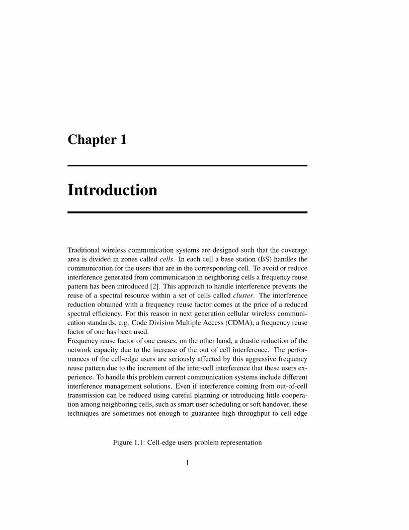
Figure 1.1: Cell-edge users problem representation
1

2 Chapter 1 Introduction
user. For that reason major standardization bodies are now including explicit in-
terference coordination strategies in next generation cellular communication stan-
dards. For example, in future releases of cellular communication standard called
Long Term Evolution Advanced (LTE-A) those techniques are grouped in what is
called Coordinated Multipoint transmission and reception techniques [3]. These
techniques are based on more interference-aware base station cooperation. The
most recent evolutions of this particular cooperative communication technique is
the so called Network or virtual MIMO (Multiple-Input-Multiple-Output), where
the main concept is to introduce a deeper collaboration between neighboring BSs
such that each user is served by multiple BSs. This scenario can be thought as
a distributed MIMO broadcast (BC) channel. For comprehensive introduction on
recent results on this topic please refer to [4]. To achieve this result all the BSs
should be connected to a centralized processing/control unit because full coopera-
tion at the signal-level is required, in particular all the BSs should be aware of all
the messages destined to all users in the network. These cooperative techniques, in
their implementation in LTE-A, have been shown to bring a significant improve-
ment in spectral efficiency for cell-edge users, while the resulting gain for full cell
coverage is almost negligible [5]. Although very useful, at least to improve the
cell-edge users performance, these techniques introduce some challenges in real
systems. Realizing the required cooperation and coordination among different BSs
poses different problems in real systems with limited backhaul capacity and finite
latency.
1.1 Interference channel: Overview
A different way of looking at the cell-edge users problem is to mathematically de-
scribe the setting as a K-user interference channel. In this system model K pairs
of transmit and receive devices transmit in the same frequency resource. Each
transmitter wishes to communicate only to the corresponding receiver, then each
communication generates interference to the K − 1 non intended receivers. This
system model differs from the Network MIMO approach because the level of co-
operation between transmitters stops at the channel state information (CSI). Hence
less signaling is required between BSs. In particular, according to the used trans-
mission technique, different degrees of channel knowledge are exchanged between
transmitters.
Interference channel has been the focus of intense research over the past few
decades, starting from the celebrated paper by Carleial [6]. From an information-
theoretic point of view its capacity region, intended as all the possible rate tuples
that can be simultaneously achieved by all users, in general remains an open prob-

1.1 Interference channel: Overview 3
lem and is not well understood even for simple cases. In [7] the counterintuitive
result that if the interference is strong enough (called strong interference regime)
the interference does not limit the performances of a two user interference chan-
nel is reported. This shows that exploiting the interference instead of treating it as
noise is the optimal strategy. The other known results is that treating the interfer-
ence as noise is optimal in the weak interference regime. In [8] the authors show
that even for the 2−users system, the most studied case, to achieve the system
capacity within one bit very complicated transmission schemes are required, that
should be adapted to the particular interference regime of the system. To achieve
this result the author use Han-Kobayashi [9] type scheme. This coding scheme is
based on splitting the transmitted information of both users in a private message,
that can be decoded only at the intended receiver, and a common message, that can
be decoded at both receivers. The key innovation here is modulating the power of
the private message such that the corresponding received signal is at the level of
noise. In this way the interference generated at the non intended receiver can be
neglected.
1.1.1 MISO Interference Channel
With the introduction of multiple antennas at the receiver, the so called single-
input-multiple-output (SIMO) systems, it is possible to increase the achieved ca-
pacity [2], if the receiver has proper channel knowledge (CSIR). This results is
due to the power gain achieved by combining all the received signal from all the
receiving antennas. A similar result can be obtained if the transmitter is equipped
with multiple antennas, system called multiple-input-single-output (MISO). In this
case if the transmitter has channel state information (CSIT) then a power gain is
achieved also for MISO systems. These simple results can be also extended to
more complex systems where a transmitter wants to communicate with multiple
receivers at the same time [10]. Also the capacity of an interference channel has
been investigated when either the transmitter or the receiver is equipped with mul-
tiple antennas. For example in [11] the capacity of a two user MISO/SIMO inter-
ference channel is studied providing the capacity region for a class of MISO IFC
in the strong interference regime. A new outer bound is also provided for a general
MISO IFC, but the capacity for a more general interference channels, with arbi-
trary number of users, is still an open problem. Then, more practical approaches
were introduced for system performance optimization using linear transmitters and
receivers. In [12, 13] the beamformers for a K-user MISO IFC are determined to
minimize the total transmit power imposing a set of per user Quality of Service
(QoS) requirements at each receiver. [14, 15] address the similar problem of max-
imizing the minimum Signal to Interference plus Noise ratio (max min SINR) for

4 Chapter 1 Introduction
the MISO IFC.
In [16, 17, 18] distributed solutions for the BF design problem are investigated,
where the main objective is to reduce the signaling exchange between pairs of
users. Some of the techniques use concepts from game theory to describe the
proposed algorithms.
A different line of research can be found in [19, 20, 21, 22] where the objective
is the characterization of the rate region of a MISO IFC where linear processing
is used at the transmit side. The region under investigation is defined as the set
of rate tuples that can be simultaneously achieved by the transmitting pairs. The
main focus of this analysis is the definition of the Pareto boundary of the capacity
region, defined as the set of points where the performance of one user can not be
incremented without reducing the performance of other users.
1.1.2 MIMO Interference Channel
With the discovery that using multiple antennas at both transmitter and receiver can
bring a significant increase of the system throughput [23], multiple-input-multiple-
output (MIMO) communication has been widely applied to all communication sys-
tems, including the interference channel.
Interference Alignment
As we have already seen the problem of finding the capacity of an interference
channel is a difficult problem that has not been completely solved yet. The prob-
lem becomes even more complicated with the introduction of MIMO pairs in the
interfering network. To simplify the problem a different approach has been recently
introduced. The focus now becomes the rate approximation at high signal-to-noise-
ratio (SNR). In that regime the sum rate rate curve can be completely described
using the prelog factor, also called degrees of freedom (DoF):
C(ρ) = d log(ρ) + o(log(ρ))
where C(ρ) represents the sum capacity, ρ is the SNR and d is the pre-log factor.
It can be interpreted as the number of interference free dimensions available in the
system. It can also be defined as:
d = limρ→∞
C(ρ)
log(ρ)
It was introduced in [24] for a single user MIMO link and it became immediately
instrumental also for more complex systems. For a 2-user MIMO IFC the achiev-
able DoF was studied in [25], for interference channel with more users the use of

1.1 Interference channel: Overview 5
Interference Alignment (IA) becomes instrumental [26, 27]. In [28] the authors
have demonstrated the achievability of a capacity prelog factor of K/2 in a K-user
SISO interference channel, then half the DoF of an interference free network can
be achieved. The key idea behind interference alignment is to process the transmit
signal (data streams) at each transmitter, so as to align all the undesired signals at
each receiver in a subspace of suitable dimensions. The MIMO interference chan-
nel is more difficult to handle and some recent results on DoF for this case are
reported in [29, 30]. Even though IA has the promising property to maximize the
DoF, a closed form expression for the beamforming filters is not known in general.
In [31, 32] a solution is proposed for K-user MIMO IFC where each pair of users
is equipped with N = K − 1 antennas. To find an IA solution for more general
system configurations iterative algorithms should be used [33, 34, 35, 36], where
different cost functions are used to determine a set of IA beamformers using nu-
merical solutions. These algorithms can be also used to evaluate the existence of
an IA solution through simulations. The existence of an IA solution for MIMO IFC
has been studied in several papers [37, 38, 39] where different sets of conditions
are to be satisfied by a K-user MIMO IFC to admit an IA solution.
Sum Rate Maximization
The objective of IA transmission is to maximize the DoF that represents a good
approximation of the rate curve at high SNR. The same concept cannot be applied
at medium and low SNR regimes, for this reason IA manifests poor performances
in these SNR regimes. Hence different approaches have been proposed to design
the transmit and receive filters in a K-user MIMO IFC. One possible approach is
the maximization of the sum rate. In the seminal work [40] the authors noted that
the network capacity in general is neither a convex nor concave function of the
transmit covariance matrices and hence its optimization is a difficult problem. The
game theoretic approach was used in [41] to study the MIMO IFC modeling the
problem as a non-cooperative game. The proposed solution is proved to achieve a
Nash equilibrium but this point can be very far from the optimal sum rate point.
The weighted sum rate (WSR) maximization problem has been studied in some
recent papers [42, 43, 44]. In [42] the single stream MIMO IFC is studied, propos-
ing an iterative algorithm for the maximization of the WSR. A different approach
is used in [43] where the problem is solved using second-order-cone-programming
(SOCP). Finally in [44] the WSR maximization is achieved, in an interfering broad-
cast channel, extending the results proposed for a BC in [45]. The solution relies
on the connection between the WSR maximization and the minimization of the
weighted sum mean squared error (WSMSE).

6 Chapter 1 Introduction
Channel State Information Acquisition
To determine a set of beamformers that maximizes the DoF at high SNR, using IA,
or to maximize the sum rate, using the approaches described above, different forms
of channel state information (CSI) are required. In most of the cases CSI at both
terminals, transmitter and receiver, is needed to achieve the proper joint design of
the transmit and receive filters. This is usually acquired using some training and
feedback phases between transmitters and receivers. The problem of how feedback
influences the IA beamforming design was studied in [46, 47, 48]. In [46, 47],
using quantized channel feedback, it is shown that full multiplexing gain can be
achieved if the feedback bit rate scales sufficiently fast with the SNR. The authors
of [48] introduce analog feedback for the acquisition of full CSIT. They show that
using analog feedback, for acquisition of CSIT and IA beamforming design, incurs
no loss of multiplexing gain if the feedback power scales with the SNR. In [49] a
staggered block fading channel model is the only assumption required to achieve
IA. The resulting multiplexing gain is much lower however than for the case of
full CSI. These techniques are now known by the terms delayed CSIT (DCSIT)
or retrospective IA. The problem of studying the maximum DoF achievable using
DCSIT has recently attracted a lot of research effort. [50, 51] introduced a new
transmission protocol that maximizes the achievable DoF in a BC channel. In [52]
the authors extend the results from [50] to the two user MISO IFC.
1.2 Cognitive Radio
Spectrum regulatory bodies, since their foundation at the beginning of the 20th
century, have allocated portions of the frequency spectrum to different wireless
services in a fixed and static way. This has been done with the objective of avoid-
ing/reducing the possibility to generate interference. With the rapid growth of
wireless services the fixed frequency allocation policy, used until now, has been
demonstrated to be very inefficient in term of spectral utilization. In addition al-
most all of the frequency bands have been already assigned, Fig. 11.2. The conse-
quent spectrum scarcity has a significant effect on wireless communication service
providers since nowadays the frequency bands are assigned to the highest bidder
in public auctions, then the frequency acquisition represents one of the most im-
portant cost for operators. In a recent measurement campaign [53], undertaken
by Federal Communications Commission (FCC) in the US, has shown that the
spectrum usage is typically concentrated over certain frequency bands, while a sig-
nificant amount of the licensed bands remains unused or underutilized for 90% of
time. This problem has inspired the seminal work in [54] where the concept of
Cognitive radio (CR) has been introduced. According to this new communication

1.2 Cognitive Radio 7
Figure 1.2: US frequency allocation chart, www.ntia.doc.gov/osmhome/allochrt.pdf.
paradigm, further developed in [55], a cognitive radio system is defined as a set
of intelligent devices that are aware of the surrounding environment adapting their
communication parameters with the objective of a reliable communication and a
more efficient spectrum utilization. The most common CR scenario comprises of a
set of secondary users, that represent the cognitive users, that want to coexist with
a set of primary users, the legacy spectrum holders. The most important feature of
the cognitive devices, as the name suggests, is the ability to learn the environment
and react properly. This problem gave birth to an intense line of research where the
main objective is to study how it is possible to understand if in a given frequency
band a transmission is taking place or not. This goes under the name of spectrum
sensing, refer to [56] and reference therein for a comprehensive review of major
contributions. One of the first attempt to make the CR principles a reality was the
IEEE standard 802.22, that had the objective to use TV white spaces to develop
a communicating system for wireless regional area networks (WRANs). In 2009
a new standard proposal, IEEE 802.11af, considered to modify both the 802.11
PHY and MAC layers to use TV white space. For additional information on CR
standards refer to [57].
From an information theoretic point of view, different cognitive radio commu-
nication paradigms have been introduced according to the amount of information
exchanged between primary and secondary users and the constraints imposed on
the secondary communication. In [58] the following cognitive radio communica-
tion settings are introduced: Overlay, Underlay and Interweave.
Overlay Paradigm
Overlay CR is a cooperative technique in which the secondary signals are designed
to offset any degradation they may cause to primary communications, requiring a
shared knowledge of the codebooks and modulation schemes. With this additional
information some form of asymmetric cooperation can be established. For example
the opportunistic user can split its rate dedicating part of his available transmit
power to broadcast also the message designated to the incumbent receiver. With
the remaining resources he transmits his message for private communication with
the secondary receiver. Other encoding strategies [58] can be used to settle an
overlay communication like dirty paper coding (DPC) or rate splitting. In this
scenario primary communication is not harmed or could even by improved as a
result of relaying gain. This CR setting can be also read as some combination of
broadcast and interference channels with degraded message sets [59]. Even though

8 Chapter 1 Introduction
the overlay CR is the most studied CR setting from an information theoretic point
of view, the capacity of such a system is still not known in general. It is only known
in some particular regimes. In [60] weak interference regime is studied, the authors
showed that in this regime, where the link between the cognitive Tx and primary Rx
is weak, the capacity of the overlay CR channel is achieved using a combination
of DPC and superposition coding. The cognitive user exploits the knowledge of
the primary message to encode its own message in such a way that it is received
at the cognitive receiver interference free. At the same time using superposition
coding, it uses part of its available power to convey also the primary message and
the remaining power is used for cognitive transmission. In the opposite regime,
Strong interference seen at both receivers, [61] found that the capacity of the CR
channel is achieved using superposition coding at the cognitive transmitter.
Underlay Paradigm
Underlay CR allows coexistence of a primary (usually licensed) network and a sec-
ondary (cognitive) one, constraining interference caused by secondary transmitters
on primary receivers to be under a certain threshold, usually called Interference
temperature constraint [55]. In order to attain these interference constraints dif-
ferent techniques can be used ranging from coding methods up to the use of the
spatial dimension (multiantenna systems). The problem of studying the capacity
region, of different communicating systems, constraining the received power to
some users was explored in [62], these constraints significantly change the struc-
ture of the problem. In [63] an underlay cognitive radio setting is studied in fading
environments. It is shown that a significant capacity gain can be achieved by the
opportunistic user in channels affected by severe fading, because the probability
that the cross link primary-secondary to be in fade is non negligible end hence the
secondary system can achieve a substantial rate increasing its transmitted power
without interfering significantly with the primary communication. In the under-
lay CR paradigm constraining the interference at the primary receivers is the main
objective of the cognitive transmitters. Providing the cognitive users with multi-
ple antennas enhances the capability of controlling the interference generated at
the primary receivers, for this reason the beamforming design problem in under-
lay cognitive systems has been the focus of intense research in recent years. [64]
studies the problem of maximizing the secondary user’s rate controlling the inter-
ference caused at the primary receivers. A different line of research focuses on
satisfying a minimum quality of service requirement at the cognitive users in an
underlay scenario [65, 66, 67]. There the secondary network is always modeled
as a BC channel that wants to communicate in the presence of a set of primary
receivers. In [68, 69] the objective was to optimize the sum rate of the secondary

1.3 Thesis Outline and Contributions 9
network, modeled as an interference channel, under received interference power
constraints at primary users.
Interweave Paradigm
Finally, Interweave (IW) CR exploits the unused communication resources, called
white spaces, of the primary system in an opportunistic fashion. In this commu-
nication paradigm, secondary transmission can take place only if it does not cause
any interference to the primary user. The unused primary resources can be time,
frequency or, as recently introduced, space.
The cognitive radio problem has been studied also from a game theoretic per-
spective in [70], there the authors proposed a decentralized algorithm, based on
iterative water filling, to maximize the secondary system’s performances. A deep
analytical description under the game theoretic framework is also provided. In [71]
a detailed overview on game theory and its application to CR problem is provided.
In this communication paradigm the use of multiple antennas is even more
beneficial than the underlay setting. One of the first paper studying the spatial
dimension in CR systems was [64]. Some attempts to make CR practical can be
found in [72, 73]. The authors propose an initial transmission scheme where the
primary communication is exploited in order to learn the environment and properly
design the secondary users’ beamformers. In the proposed analysis the secondary
channel estimation errors are taken into account in the secondary BF design. The
interference caused at the secondary receiver, due to primary communication, is
reduced introducing a proper receive filter at secondary receivers.
In [74] a new approach to setup a cognitive transmission has been proposed
for frequency selective channels. The authors proposed to apply a Vandermonde
precoder as transmit filter at the cognitive user, for this reason it is called Van-
dermonde Frequency Division Multiplexing (VFDM). The Vandermonde precoder
is constructed using the L roots of the L-tap channel that connects the cognitive
transmitter with the primary receiver. With this transmitter the interference to the
primary receiver is completely zeroforced. This approach has the advantage that
no cooperation is required between primary and secondary to setup an interweave
cognitive radio communication.
1.3 Thesis Outline and Contributions
This thesis is divided in two main parts. Part I focuses on the interference chan-
nel, where we first study the beamformer design problem in a MISO interference
channel introducing some duality principles, that can be thought of as an extension

10 Chapter 1 Introduction
to the IFC of the results obtained for the broadcast channel. Then the problem of
maxminSINR beamformer design is addressed. In the following chapters , intro-
ducing more antennas also at the receiver side we study the problem of joint design
of transmit-receive filters in MIMO interference channel. We study interference
alignment beamformers design, with particular focus on feasibility analysis, and
on weighted sum rate maximization. Finally the problem of channel state infor-
mation acquisition at both transmit and receive side, for solving the previously
introduced problems, is studied using analog feedback.
Part II deals with cognitive radio scenarios. At first we study the problem
of beamforming design in MISO underlay cognitive interference channel solving
the problem of power minimization under per user power constraints and limit-
ing the maximum amount of interference generated at primary users. Then in the
following chapters we introduce the concept of Spatial Interweave. In chapter 8
we describe all the transmission phases required to opportunistically design the
secondary beamformer in TDD communications. To exploit channel reciprocity,
due to TDD transmission, we also consider the calibration problem and how this
additional operation influences the design problem. We discover that calibration
between non cooperative users is not required implying that spatial interweave CR
setting is possible in practice without any cooperation between primary and sec-
ondary users. The simple setting with one primary and one secondary pair is ex-
tended to multiple secondary pairs and primary receiver in chapter 9. In this chapter
the IA design problem is studied in a CR setting where the feasibility problem is
also introduced and studied providing a set of feasibility conditions.
In the following paragraphs we give a brief overview of the thesis describing
the content of different chapters underlining their contributions.
Chapter 2 - MISO Interference Channel
In this chapter we start introducing some Uplink-Downlink (UL-DL) duality prin-
ciples, initially introduced for the BC channel, adapting them to the MISO interfer-
ence channel. Then UL-DL duality is used for the solution of the weighted SINR
(WSINR) balancing problem for MISO IFC with individual power constraints.
We introduce a new iterative algorithm that solves the WSINR balancing problem
when only one power constraint is active. Then we propose an iterative algorithm
that solves the problem in a decentralized manner when nothing can be said on
the number of active power constraints. The algorithm solves the problem using
a sequence of power minimization problems with a proper set of QoS constraints.
The research contributions of this chapter have been published in
• F. Negro, M. Cardone, I. Ghauri, and D. T. M. Slock, ”SINR balancing
1.3 Thesis Outline and Contributions 11
and beamforming for the MISO interference channel,” in Personal Indoor
and Mobile Radio Communications (PIMRC), 2011 IEEE 22st International
Symposium on, Sept. 2011.
• F. Negro, I. Ghauri, and D. T. M. Slock, ”On duality in the MISO inter-
ference channel,” in Signals, Systems and Computers (ASILOMAR), 2010
Conference Record of the Forty Fourth Asilomar Conference on, Nov. 2010,
pp. 2104 -2108.
Chapter 3 - Interference Alignment Feasibility for MIMO interference chan-
nel
The focus of this chapter is the feasibility study of interference alignment solu-
tions for constant coefficients MIMO interference channel. We first introduce the
general system model of a K-user MIMO IFC that will also be used in following
chapters. Then we provide a systematic method to check feasibility of IA solu-
tions for an arbitrary DoF allocation. We validate the proposed approach using
some numerical examples, comparing the result of our feasibility check with the
convergence property of an iterative algorithm for determining IA solutions. We
discuss interference alignment duality and the interpretation of IA as a constraint
compressed SVD. The results presented in this chapter are also published in the
following papers:
• F. Negro, S. Shenoy, D. T. M. Slock, and I. Ghauri, ”Interference alignment
limits for K-User frequency-flat MIMO interference channels,” in Proc. Eu-
ropean Signal Proc. Conf. (Eusipco), Glasgow, Scotland, Aug. 2009.
• F. Negro, S. P. Shenoy, I. Ghauri, and D. T. M. Slock, ”Interference align-
ment feasibility in constant coefficients MIMO interference channel,” in Proc.
11th IEEE International Workshop on Signal Processing Advances in Wire-
less Communications (SPAWC 2010), June 2010.
• F. Negro, I. Ghauri, and D. T. M. Slock, ”Deterministic annealing design and
analysis of the noisy MIMO interference channel,” in Information Theory
and Applications Workshop (ITA), 2011, Feb. 2011, pp. 1 -10.
Chapter 4 - Sum rate maximization for the noisy MIMO interference channel
In this chapter we introduce the weighted sum rate maximization (WSR) problem
for a MIMO interference channel. We propose a new iterative algorithm based on
the extension of the relation between WSR maximization and the minimization of

12 Chapter 1 Introduction
the weighted sum mean squared error (WMSE). Then we specify the proposed al-
gorithm when the WSR is maximized under a per-stream approach.The per-stream
approach helps us to introduce a WSR duality for the MIMO IFC where the optimal
transmit filter results to be an MMSE receiver filter in a dual UL communication
with a proper transmit covariance matrix and dual noise variance. To reduce the
possibility to converge to local optimal solution we introduce a novel approach
based on Deterministic Annealing. Finally we describe how to optimize the WSR
at high SNR. Some simulation results are provided to validate the proposed algo-
rithm numerically.
In the following papers are reported the research contributions described in this
chapter:
• F. Negro, S. Shenoy, I. Ghauri, and D. T. M. Slock, ”On the MIMO inter-
ference channel,” in Information Theory and Applications Workshop (ITA),
2010, 31 2010-Feb. 5 2010, pp. 1 -9.
• F. Negro, S. Shenoy, I. Ghauri, and D. T. M. Slock, ”Weighted sum rate max-
imization in the MIMO interference channel,” in Personal Indoor and Mobile
Radio Communications (PIMRC), 2010 IEEE 21st International Symposium
on, Sept. 2010, pp. 684 -689.
• F. Negro, I. Ghauri, and D. T. M. Slock, ”Deterministic annealing design and
analysis of the noisy MIMO interference channel,” in Information Theory
and Applications Workshop (ITA), 2011, Feb. 2011, pp. 1 -10.
• F. Negro, I. Ghauri, and D. T. M. Slock, ”Optimizing the noisy MIMO inter-
ference channel at high SNR,” in Communication, Control, and Computing
(Allerton), 2010 48th Annual Allerton Conference on, 29 2010-Oct. 1 2010,
pp. 254 -261.
Chapter 5 - Sum Rate Maximization with Partial CSIT via the Expected Weighted
MSE
In this part of the thesis we focus on robust beamforming design for a MIMO
interfering broadcast channel with the objective of maximizing the sum rate. We
assume that each transmitter has stochastic channel state information (CSI) while
the receiver has perfect CSI. The solution proposed for robust beamforming design
is based on the relationship between WSR and Weighted MSE (WMSE) introduced
for the MIMO interference channel in chapter 4. Here the optimal beamforming
filters are obtained from the minimization of the sum of average WMSE, then an
iterative algorithm is introduced to solve the problem. The performance of the

1.3 Thesis Outline and Contributions 13
proposed solution is finally validated numerically. The results described in this
chapter are published in:
• F. Negro, I. Ghauri, and D. T. M. Slock, ”Sum Rate maximization in the
Noisy MIMO Interfering Broadcast channel with partial CSIT via the ex-
pected weighted MSE,” in Wireless Communication Systems (ISWCS), 2012
IEEE 4th International Symposium on 28-31 August 2012.
Chapter 6 - CSI acquisition in the MIMO interference channel via analog
feedback
All the joint transmit-receive filter design techniques introduced in this thesis, WSR
maximization and IA, require some form of CSI at both terminals. In this chapter
we study the problem of CSI acquisition at transmit and receive side introducing
two transmission protocols that are based on channel training and analog feedback
(FB). We also study the problem of optimizing the sum rate, by focusing in partic-
ular on the resulting degrees of freedom (DoF), as a function of the coherence time.
This approach helps us to optimize the system parameters, number of transmitting
antennas and transmitted streams,considering the CSI acquisition overhead. In the
following papers are reported the results provided in this chapter:
• F. Negro, U. Salim, I. Ghauri, and D. T. M. Slock, ”The noisy MIMO inter-
ference channel with distributed CSI acquisition and filter computation,” in
Signals, Systems and Computers (ASILOMAR), 2011 Conference Record of
the Forty Fifth Asilomar Conference on, 2011.
• F. Negro, D. T. M. Slock, I. Ghauri, ”On the noisy MIMO interference chan-
nel with CSI through analog feedback,” in Communications Control and Sig-
nal Processing (ISCCSP), 2012 5th International Symposium on (ISCCSP),
2012 , pp. 1 - 6
Chapter 7 - Beamforming for the Underlay Cognitive MISO Interference Chan-
nel
Here we focus on the problem of beamformer design for a CR network modeled
as a MISO interference channel. Since we assume to work in an underlay setting
we further impose a set of interference power constraints at the primary receivers.
Extending the results on UL-DL duality to cognitive radio settings we design the
beamformer at the secondary transmitters in order to minimize the total transmitted
power. We propose an iterative algorithm that efficiently solves the power mini-
mization problem, at the secondary network, while a set of interference constraints
14 Chapter 1 Introduction
are imposed on the primary receivers. The research contributions in this chapter
are reported also in the following paper:
• F. Negro, I. Ghauri, and D. T. M. Slock, ”Beamforming for the underlay cog-
nitive MISO interference channel via UL-DL duality,” in Cognitive Radio
Oriented Wireless Networks Communications (CROWNCOM), 2010 Pro-
ceedings of the Fifth International Conference on, June 2010, pp. 1 -5.
Chapter 8 - Spatial Interweave TDD Cognitive Radio Systems
In this chapter we study the joint optimization of the transmit-receive filters in
a spatial interweave cognitive radio channel, we describe all the communication
phases required to acquire the necessary information at primary and secondary
users. We focus in particular on how to really exploit channel reciprocity in real
TDD transmission using UL DL channel calibration studying how calibration in-
fluences transmit and receiver filter design at primary and secondary devices. An
important result that comes out of our analysis is that calibration between non co-
operative Tx and Rx is not needed for secondary beamformer design. We introduce
an extension of the results to the case with multiple primary transmitter and receiver
pairs. If the primary network designs its beamformers according to IA, thanks to
IA duality, the secondary pair can blindly estimate the DL received subspace at all
primary receivers from the transmitted signal subspace in the UL communication.
Calibration issues are also studied in this setting proving that calibration between
non cooperative users is not required also in the extended scenario. The results
described in this chapter are partially published in:
• F. Negro, I. Ghauri, and D. T. M. Slock, ”Transmission techniques and chan-
nel estimation for spatial interweave TDD cognitive radio systems,” in Pro-
ceedings of the 43rd Asilomar conference on Signals, systems and comput-
ers, Asilomar’09, 2009, pp. 523-527.
Chapter 9 - Spatial Interweave Cognitive Radio Interference Channel with
Multiple Primaries
In this part of the work we consider a secondary network modeled as a K-user
MIMO IFC that wants to communicate in presence of L primary multi antenna
receivers. The secondary users’ beamformers are designed according to IA with
the additional interweave constraints to generate an interference subspace, at each
primary receiver, with given dimension. We study the feasibility of an IA solution
in the cognitive radio system under investigation based on the results presented in
chapter 3. Then we propose an iterative algorithm that finds the secondary users’

1.3 Thesis Outline and Contributions 15
transmit and receive IA filters satisfying the interweave constraints at the primary
receivers. The contributions of this chapter can be found in the following paper:
• F. Negro, I. Ghauri, and D. T. M. Slock, ”Spatial interweave for a MIMO
secondary interference channel with multiple primary users,” in 4th Interna-
tional Conference on Cognitive Radio and Advanced Spectrum Management,
(CogART 2011), October 2011.

Part I
Interference Channel
Chapter 2
MISO Interference Channel
2.1 Introduction and State of the Art
In this first part of the thesis we focus on the K-user interference channel (IFC)
where pairs of users want to communicate between each other without exchang-
ing (data) information with non-intended pairs. Interference at each user is treated
as additional Gaussian noise contribution and hence linear beamforming process-
ing is optimal. This, in the information theoretic sense, is the noisy interference
channel. In particular, in this chapter, we focus on the case where the transmitters
are equipped with multiple antennas and they communicate with single antenna
receivers. This setting has been labeled as MISO (multiple-input-single-output) in-
terference channel [11]. As already discussed the IFC, and in particular the multi-
antenna case, can be used to model interesting realistic problems, like cell-edge
users problem or coexistence of macro-femto cells, that has attracted a lot of re-
search attention in recent years. The first attempt to study the MISO IFC has been
to port the solutions and methods applied to the broadcast or multiple access chan-
nels to the IFC, but as we will see this is not always a straightforward process.
The first important tool that has been used to solve transmission problem is up-
link/downlink (UL/DL) duality.
UL-DL duality is a well-established tool for the study of the traditional Broad-
cast (BC) channel. For example it has been recently used [75] [76] to solve the BC
beamforming and power allocation problem. Using this duality, the BF designed in
the virtual (dual) uplink communication can be used in the actual downlink prob-
17

18 Chapter 2 MISO Interference Channel
lem to achieve the same SINR values by choosing appropriate downlink power
allocations. The authors give a set of conditions for duality in a BC channel and
relate feasibility of the DL problem with the one of the corresponding UL that
is normally easier to be solved. In the seminal work [77] a duality between the
achievable rate region for the MIMO BC and the capacity region of the MIMO
multiple-access channel (MAC), which is easy to compute, has been introduced.
The authors showed that the dirty paper region [78] of a MIMO BC is exactly
equal to the capacity region of the dual MIMO MAC, with all the transmitters hav-
ing the same sum power constraint as the MIMO BC. With this new duality theory
the computational complexity to compute the rate region for a MIMO BC channel
has been reduced.
The multicell problem, that we call the interference channel, is more complex
to handle due to the per-user (per BS) power constraints. [12] addresses duality in
a similar setting, which the authors call the multicell setting, where previous re-
sults on interpretation of UL-DL duality as Lagrangian duality are exploited. [12]
then solves the power minimization problem subject to Quality of Service (QoS)
constraints and per base station power constraints formulated as weighted total
transmit power. In [79] the authors establish the uplink-downlink beamforming
throughput duality with per-base station (BS) power constraints for a multi-cell
system. The objective is to provide a more solvable form for optimal downlink
beamforming in the multi-cell environment. They found that the optimal downlink
beamforming reveals to be the minimum mean squared error (MMSE) beamform-
ing in the dual uplink. Even though the results are given for MISO system the
extension to the MIMO case is not provided.
The maxmin SINR beamforming problem formulation satisfies a fairness re-
quirement because at the optimum all the SINRs are equal, for this reason it is
also called SINR balancing problem. Balancing the SINR implies that the system
performances are limited by the weak users causing a reduction of the overall sum
rate. This problem has been extensively studied initially in the single cell broadcast
channel. In the original works [80] and [81] the problem of signal-to-interference
ratio (SIR) balancing problem, for MISO BC channel is studied. More recently the
same problem is studied in [82] within the general framework of invariant interfer-
ence functions studying the condition for existence and uniqueness of the solution.
The more general SINR balancing problem has been studied in [76] for single cell
Broadcast (BC) channel under the sum power constraint using the well-established
tool of UL-DL duality [77].
In [83] the authors study the weighted SINR balancing problem for a MIMO
BC channel. They show that the problem can be solved efficiently and optimally
for rank one channel. An extension of the proposed algorithm, that converges to
a local optimal solution, for general channel matrices, is studied. In this paper the

2.1 Introduction and State of the Art 19
MIMO problem is solved working with a per-stream SINR approach.
[15] investigates the max min SINR problem for multicell multi user MISO system
based on long term channel state information where only one user is scheduled
in each cell. This makes the system essentially an interference channel, the only
difference is that the authors consider a sum power constraint instead of the more
realistic per BS power constraints. They propose an iterative algorithm to solve
the problem based on UL-DL Lagrange duality. The SINR balancing problem in
the MISO IFC has been studied, under general power constraints, in a recent paper
[84] where only power optimization has been considered. In [14] the authors stud-
ied the beamforming design problem for SINR balancing for the multiuser multi-
cell scenario under per base station power constraints. Their solution is based on
the equivalence between the SINR balancing problem and the power minimization
problem. The iterative algorithm that they derive solves the problem in a central-
ized fashion.
Similar problems have been studied in some recent papers with the objective of
Pareto rate region characterization. The Pareto boundary is defined as the set of
points where the performance of one user can not be incremented without decre-
menting the performance of other users. From the definition we see the importance
of solutions that fall on the Pareto boundary because they are the solutions that
efficiently exploit the transmission resources. In particular in [20] the two user
MISO interference channel Pareto boundary characterization is considered. They
propose a method based on solving the problem as a sequence of second order cone
programming feasibility problems. A recent paper [22] applies a similar parame-
terization of the Pareto boundary for the more general setting of the multicell DL
system. The system setup introduced in that paper can model, as extreme cases,
the MISO IFC and a network MIMO systems.
In the seminal work [19] the problem of the Pareto characterization is described
for a K-user MISO IFC. The main result is that the linear transmitters that allow
to achieve the Pareto boundary are described as a linear combinations of channel
vectors and they should carry all the possible transmit power. This parametriza-
tion requires a total of K(K − 1) complex parameters. This result has a more
intuitive explanation if particularized for a 2-users IFC. In this case the BF vector
should be a linear combination of zero-forcing (ZF) and maximum ratio transmit-
ter (MRT). This means that the Pareto optimal points are obtained with BFs that
represent a good compromise between a selfish transmit strategy, represented by
the MRT solution, and a more altruistic solution, the ZF BF. In [85] the prob-
lem of Pareto region characterization is more completely studied under the Game
Theoretic framework but specialized for the two users case. Recently in [21] a new
parametrization has been introduced, based on the introduction of interference tem-
perature constraint. This concept has been borrowed from cognitive radio [58] that

20 Chapter 2 MISO Interference Channel
essentially describes the level of interference received at each receiver. In this new
parametrization of the Pareto boundary K(K − 1) real parameters are required. In
[22] this value has been reduced to 2K − 1 optimizing a proper function of the
SINRs.
In [86] the author consider the Pareto characterization for the multi-cell multi-
user setting introducing the concept of power gain region defined as the region
of all jointly achievable power gains at the receivers. They show that the Pareto
optimal points are achieved with rank-1 covariance matrices and the corresponding
BF vectors can be parameterized using T (K− 1) real-valued parameters, where Tis the number of transmitters. The power gain region results to be a convex region
and the point on the boundary can be achieved using simple BF vectors. The same
authors in [87] have introduced a new characterization for the Pareto boundary of
the 2-user MISO IFC using game theory concepts coming from economic theory
determining a single real-valued parametrization. The novelty is that they cast
the problem as a pure exchange economic problem where each link is seen as a
consumer that can exchange goods to maximize their utility. In the MISO IFC
goods are the beamforming vectors and the utility the SINRs. In the recent paper
[88] the authors study the Pareto boundary of the rate region of a 2 user MIMO
interference channel with single beam transmission proposing an efficient iterative
method for its numerical computation.
2.2 Contributions
In this chapter we first revisit some of the UL-DL duality principles, introduced
for the BC channel in [75], for the MISO interference channel. We show that the
results that are valid in the BC channel can be easily extended to the IFC for the
case of total sum power constraint. A short introduction of the UL-DL Lagrange
duality for the MISO IFC under per BS power constraint is provided based on the
recent results in [12]. This theory will then be used for the solution of the weighted
SINR (WSINR) balancing problem for MISO IFC. We then study the WSINR
balancing problem for a MISO IFC with individual power constraints introducing
some interesting consideration on power allocation at the optimal solution. Since
in the MISO IFC with per BS power constraints, a subset of users always trans-
mits with full power according to the antenna distribution and number of users in
the system, we propose a new iterative algorithm that solves the WSINR balanc-
ing problem when only one power constraints is active. Subsequently we study
the problem in a more general setting and we propose an iterative algorithm that
solves the problem in a decentralized manner. This solution is based on the relation
between the SINR balancing problem and the power minimization problem under-

2.3 System model of MISO interference channel 21
lined in [14]. We solve the maxminWSINR problem using a sequence of power
minimization problems where the QoS constraints in the beamforming problem
are increased gradually until an infeasible point is found. Then, using bisection
method, the optimal solution is determined.
Finally we show that is possible to characterize the entire Pareto boundary of
the SINR region for a general K-user MISO IFC solving a sequence of Weighted
SINR problems. Thanks to the one to one logarithmic relation between SINR and
Rate we can then characterize the Pareto boundary of the Rate region for a general
K-user MISO IFC. The basis of this characterization has been studied in [89] for
a single-input single-output (SISO) IFC. Here we extend their results to the MISO
IFC. A similar results has been also recently introduced in [22].
2.3 System model of MISO interference channel
Figure 2.1: MISO Interference Channel
Fig. 2.1 depicts a K-user MISO IFC with K transmitter-receiver (Tx-Rx) pairs.
The k-th BS is equipped with Mk transmit antennas and k-th mobile user (MU)
is a single antenna node. The k-th transmitter generates interference at all l 6= kreceivers. Assuming the communication channel to be frequency-flat, the received
signal yk at the k-th receiver can be represented as
yk = hkkxk +
K∑
l=1l 6=k
hklxl + nk (2.1)
where hkl ∈ C1×Ml represents the channel vector between the l-th transmitter and
k-th receiver, xk is the CMk×1 transmit signal vector of the k-th transmitter and
nk represents (temporally white) AWGN with zero mean and variance σ2k. Each
entry of the channel matrix is a complex random variable drawn from a continuous
distribution.
We denote by gk, the CMk×1 beamforming (BF) vector of the k-th transmitter.
Thus xk = gksk, where sk represents the independent symbol for the k-th user
pair. We assume sk to have a temporally white Gaussian distribution with zero
mean and unit variance. In the SIMO UL channel the k-th BS applies a receiver
f k to suppress interference and retrieves its desired symbol. The output of such a

22 Chapter 2 MISO Interference Channel
receive filter is then given by
rk = fHk hkksk +
K∑
l=1l 6=k
fHk hklsl + f
Hk nk (2.2)
where we denoted with (.) all the quantities that appear in the UL in order to
differentiate with the same quantities in the DL.
2.4 UL-DL duality in MISO/SIMO Interference Channel
Under Sum Power Constraint
In this section we derive UL-DL duality for a MISO IFC under a total power con-
straint. To simplify the following analysis henceforth we assume that each receiver
is characterized by the same noise variance, so σ2k = σ2, ∀k and the beamforming
vectors, gk ∀k, are unit norm. The received signal for the MISO DL IFC at the k-
th mobile station is reported in (2.1) and from there we can write the corresponding
SINR as:
SINRDLk =
pkgHk hH
kkhkkgk∑l 6=k plg
Hl hH
klhklgl + σ2(2.3)
where pk is the Tx power at the BS for the stream intended to the k-th user. Im-
posing a set of DL SINR constraints at each mobile station: SINRDLk = γk it is
possible to rewrite equation (2.3) in matrix notation:
Φp+ σ = D−1p (2.4)
where the two matrices Φ and D are defined in (2.5) and (2.6), p = [p1, . . . , pK ]T
and σ = σ21 are two vectors that contain all the Tx powers and and the noise
variances respectively. Vector 1 is a column vector of dimensions K × 1 that
contains all ones. In addition we define:
[Φ]ij =
{gHj hH
ijhijgj , j 6= i
0, j = i(2.5)
D = diag{ γ1
gH1 hH
11h11g1
, . . . ,γK
gHK hH
KKhKKgK
}. (2.6)
We can determine the Tx power solving (2.4) w.r.t. p obtaining:
p = (D−1 −Φ)−1σ (2.7)

2.4 UL-DL duality in MISO/SIMO Interference Channel Under Sum Power Constraint23
Now we study the SIMO UL IFC focusing in particular on the corresponding SINR.
Due to channel reciprocity we have that hkl = hHlk ∀k, l and the receive filter in
the UL is the reciprocal of the transmit filter of the DL f k = gk, ∀k. Using the
received signal in the UL channel in (2.2), the SINR for the UL channel can be
written as:
SINRULk =
qkgHk hH
kkhkkgk
gHk (∑
l 6=k qlhHlkhlk + σ2I)gk
(2.8)
where qk represents the UL Tx power from the k-th MU. Imposing the same set of
SINR constraints in the DL also in the UL: SINRULk = γk it is possible to rewrite
(2.8) as:
Φq+ σ = D−1q (2.9)
where D is defined as in (2.6), q = [q1, . . . , qK ]T and
[Φ]ij =
{gHi hH
jihjigi, j 6= i
0, j = i(2.10)
the power vector can be found as:
q = (D−1 −Φ)−1σ (2.11)
Comparing the definition in (2.5) and (2.10), we can see that Φ = ΦT . This
implies that there exists a duality relationship between the DL MISO and UL SIMO
interference channels.
It is also interesting to note that there is a strong parallel between the equations
reported above, to show the duality in the MISO interference channel, and the ones
used to prove duality in a BC-MAC in [75].
If we stack all the beamformers and the channel vectors in a matrix form, the
cascade of channel and BF can be written as:
HG =
h11 h12 · · · h1K
h21 h22 · · · h2K
.... . .
...
hK1 hK2 · · · hKK
g1 0 · · · 00 g2
. . ....
.... . . 0
0· · · 0 gK
=
h11g1 h12g2 · · · h1KgK
h21g1 h22g2
......
. . . hK−1KgK
hK1g1 · · · · · · hKKgK
(2.12)

24 Chapter 2 MISO Interference Channel
where G is a block diagonal matrix and the diagonal blocks are the BF column
vectors at different BSs. Making the notation in (2.12) more compact, denoting the
i-th row of H as Hi and the j-th column of the BF matrix as Gj , we have:
HG =
H1
H2
...
HK
[
G1 G2 · · · GK
]
=
H1G1 H1G2 · · · H1GK
H2G1 H2G2
......
. . . HK−1GK
HKG1 · · · · · · HKGK
(2.13)
If we assume that vector Hi represents the channel between all the BSs and the
i-th MU and vector Gi is the corresponding BF, equation (2.13) can be used to
represent the BC. The difference is that the BF used for an IFC has a block structure
where some blocks are zero while in the BC the BF matrix is full. This makes the
parallel between a BC and an interference channel more clear. In a similar fashion
it is possible to describe the same parallelism between the BC and the interference
channel for the UL SIMO IFC using similar matrix notation.
With the previous observations it is possible to extend the results obtained for
the UL-DL duality in the BC-MAC to the IFC under a sum power constraint.
A set of SINRs γ1, . . . , γK is feasible whenever there exists a positive power
allocation such that (2.4) for the DL ((2.9) for the UL) is fulfilled. In [75] the
following is proved for the BC-MAC duality but it is also valid for the IFC:
Targets γ1, . . . , γK are jointly feasible in UL and DL if and only if the spectral
radius ρ of the weighted coupling matrix satisfies ρ(DΦ) < 1.
Because ρ(DΦ) = ρ(DΦT ) target SINRs are feasible in the UL if and only
if the same targets are feasible in the DL. The power allocation vectors that satisfy
those constraints can be found using (2.7), for the DL, and (2.11), for the UL.
In addition the total required UL power qtot =∑
i qi is the same as the DL
power ptot =∑
i pi, this can be simply shown as follows:
∑i qi = 1Tq = σ1T (D−1 −ΦT )−T1
= σ1T (D−1 −Φ)−11 =∑
i pi(2.14)
According to the relationship (2.14) it is possible to state that both UL and DL
have the same SINR feasible region under the same sum-power constraint, i.e.,
target SINRs are feasible in the DL if and only if the same targets are feasible in

2.5 UL-DL duality in MISO/SIMO Interference Channel Under per User Power Constraint25
the UL.
Using the results obtained before it is possible to extend some beamforming design
techniques that use the BC-MAC duality to the beamforming design for a MISO
IFC.
2.5 UL-DL duality in MISO/SIMO Interference Channel
Under per User Power Constraint
In the MISO interference channel if the problem of BF design is formulated under
the sum power constraint we have shown that there exist an UL-DL duality that
can be used to solve the problem. Even though the sum power constraint is analyt-
ically attractive such constraint is not enough in a practical interference channel.
In reality each user is subject to a per user power constraint that the transmit power
can not violate. For this reason in this section we briefly describe an alternative BF
design problem that still minimizes the total Tx power but imposing also per user
power constraints. This problem has been studied for a multicell case, of which
the IFC is a special case in [12]. There an UL-DL relation, based on Lagrangian
duality for BC channel [90], has been extended to the multicell case to solve the
beamformer optimization problem.
Assuming that the SINR constraints are such that there exist at least a feasible
solution to the problem, the beamformer optimization problem now becomes:
ming1,...,gK
∑Kk=1 g
Hk gk
s.t. gHk gk ≤ Pk; k = 1, . . . ,K
SINRDLk =
gHk hH
kkhkkgk∑l 6=k gH
l hHklhklgl+σ2
k
≥γk; k = 1, . . . ,K
(2.15)
where Pk represents the maximum Tx power for user k. This problem at first sight
seems to be non convex due to the SINR constraints. For a downlink BC channel it
has been shown in [91] that this set of constraints can be transformed into a second
order cone constraint that allows for simple convex optimization solutions [92].
The Lagrange dual of the DL beamforming problem (2.15) can be rewritten as
an equivalent UL optimization problem [12], Fig.2.2, for the Rx filter:
Figure 2.2: MISO Interference Channel
fk = (∑
l 6=k
λlhHlkhlk + ηkI)
−1hHkk (2.16)
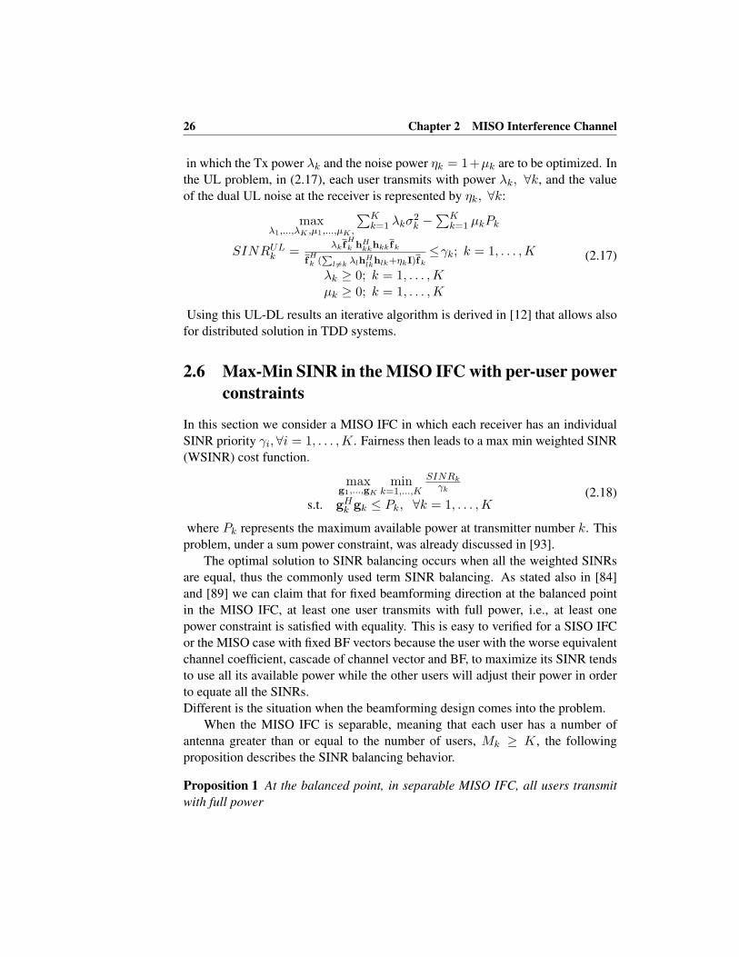
26 Chapter 2 MISO Interference Channel
in which the Tx power λk and the noise power ηk = 1+µk are to be optimized. In
the UL problem, in (2.17), each user transmits with power λk, ∀k, and the value
of the dual UL noise at the receiver is represented by ηk, ∀k:
maxλ1,...,λK ,µ1,...,µK ,
∑Kk=1 λkσ
2k −
∑Kk=1 µkPk
SINRULk =
λkfHk hH
kkhkkfk
fHk (
∑l 6=k λlh
Hlkhlk+ηkI)fk
≤γk; k = 1, . . . ,K
λk ≥ 0; k = 1, . . . ,Kµk ≥ 0; k = 1, . . . ,K
(2.17)
Using this UL-DL results an iterative algorithm is derived in [12] that allows also
for distributed solution in TDD systems.
2.6 Max-Min SINR in the MISO IFC with per-user power
constraints
In this section we consider a MISO IFC in which each receiver has an individual
SINR priority γi, ∀i = 1, . . . ,K. Fairness then leads to a max min weighted SINR
(WSINR) cost function.
maxg1,...,gK
mink=1,...,K
SINRkγk
s.t. gHk gk ≤ Pk, ∀k = 1, . . . ,K
(2.18)
where Pk represents the maximum available power at transmitter number k. This
problem, under a sum power constraint, was already discussed in [93].
The optimal solution to SINR balancing occurs when all the weighted SINRs
are equal, thus the commonly used term SINR balancing. As stated also in [84]
and [89] we can claim that for fixed beamforming direction at the balanced point
in the MISO IFC, at least one user transmits with full power, i.e., at least one
power constraint is satisfied with equality. This is easy to verified for a SISO IFC
or the MISO case with fixed BF vectors because the user with the worse equivalent
channel coefficient, cascade of channel vector and BF, to maximize its SINR tends
to use all its available power while the other users will adjust their power in order
to equate all the SINRs.
Different is the situation when the beamforming design comes into the problem.
When the MISO IFC is separable, meaning that each user has a number of
antenna greater than or equal to the number of users, Mk ≥ K, the following
proposition describes the SINR balancing behavior.
Proposition 1 At the balanced point, in separable MISO IFC, all users transmit
with full power

2.6 Max-Min SINR in the MISO IFC with per-user power constraints 27
Proof: To prove the above statement consider, without loss of generality, a K = 2user MISO IFC with Mk ≥ 2. Assume that the optimal solution of the SINR
balancing problem is given for g⋆1 and g⋆
2 where only transmitter 1 transmits with
full power, ‖g⋆1‖2 = P1, ‖g⋆
2‖2 < P2. Because Tx2 has an excess of power the
BF of user 1 can be modified s.t.:
‖g′
1‖2 = ‖g⋆1‖2 ; |h11g
′
1|2 > |h11g⋆1|2.
This new choice of BF for user 1 increases its SINR but at the same time causes a
reduction of the SINR of the other user: SINR2(g′
1,g⋆2) < SINR1,2(g
⋆1,g
⋆2) <
SINR1(g′
1,g⋆2). Tx2 to compensate for the additional interference caused by the
new BF g1 has to increase the transmitted power using a BF of the form:
g′
2 = g⋆2 + δh⊥
12
‖g′
2‖2 > ‖g⋆2‖2 ; |h22g
′
2|2 > |h22g⋆2|2
where h⊥12 is any vector that belongs to the orthogonal complement of h12 and δ
is a complex scaling factor. The choice of δ should be s.t. SINR1(g′
1,g′
2) =SINR2(g
′
1,g′
2). With this choice of g′
2 we can rise the useful signal power for
user 2 without increasing the interference caused to the non intended receiver.
With the new set of beamformers both the SINRs are increased SINR1,2(g′
1,g′
2) >SINR1,2(g
⋆1,g
⋆2). This means that the original BF vectors were not optimal hence
both users should transmit with full power.
This result is in line with what has been previously proposed in literature. As
we will see WSINR balancing problem is a possible way to characterize the Pareto
boundary of the SINR/Rate region. In [85, 86] it has been shown that the Pareto
optimal solutions are achieved transmitting with full power if Mk ≥ K, as we can
see our result also confirm this approach.
Different is the situation in low SNR regime. Here we can state that the optimal
transmission strategy for each user is to maximize the useful signal component. No
matter how strong interference becomes, noise remains the dominant impairment.
Hence the optimum transmission strategy is to beamform to match the direct link
(maximum ratio BF) at each Tx. In this case the user with the worse direct link
channel transmits with full power to maximize its SINR, which is also the sys-
temwide worst SINR. This is true also for separable MISO channel, regardless the
number of transmitting antennas.
It may be argued that different optimal points to the SINR balancing problem may
exist at low SNR. In this situation each user can be thought as decoupled from the
others, due to the high noise power. Once the system worst SINR is maximized the
max min problem is solved. The remaining users can now decide to use their power
in many different ways. For example they can use the minimum power such that

28 Chapter 2 MISO Interference Channel
all the SINRs are balanced or they can use full power to maximize all the SINRs.
Which solution should be used depends on a possible secondary objectives. If the
total power should be minimized then the balanced SINR solution is the optimal
one.
2.6.1 DL power allocation optimization
For cases where a zero forcing solution is not possible (Mk < K, ∀k) only one
user has its power constraint active. In this case for fixed BF vectors the corre-
sponding power allocation vector can be found solving an eigenvalue problem [76]
imposing only one power constraint to be active. At the optimum all the weighted
SINRs are equal. Denoting with τ the optimal value of the ratio SINR over target
QoS we can write:1
τp = DΦp+Dσ (2.19)
where matrices Φ and D are defined as in equation (2.5) and (2.6) respectively.
Assuming now that the j−th power constraint is the only one satisfied with equality
and multiplying both sides of the previous equation by xTj = 1
Pjej , where ej is a
vector with 1 only in position j, we get:
1
τ= xT
j DΦp+ xTj Dσ (2.20)
Introducing the compound matrix:
∆j =
[DΦ Dσ
xTj DΦ xT
j Dσ
](2.21)
the extended vector p = [p 1]T , and using the results from the nonnegative ma-
trix framework [94] the solution of the WSINR balancing problem w.r.t. the power
optimization is given by: τ = 1λmax(∆j)
. The power vector is the corresponding
positive eigenvector with the (K + 1)−th entry normalized to one. This approach,
that allows to extend the known result from SIR balancing to SINR balancing, is
called Bordering Method, it was introduced by [94] and then used in [76] for BC
channel. A different approach to handle noise in the SINR balancing problem is
to transform (2.19) into an homogeneous system of linear equations. This method
is based on considering a rank one modification of the matrix DΦ that leads to
the same solution obtained using the bordering method. The fact that the j−th
power constraint is active: xTj p = 1 allows us to modify WSINR balancing prob-
lem in order to obtain an unconstrained optimization problem in terms of powers.
Introducing a reparametrization of the Tx power vector:
p =1
xTj p
p (2.22)
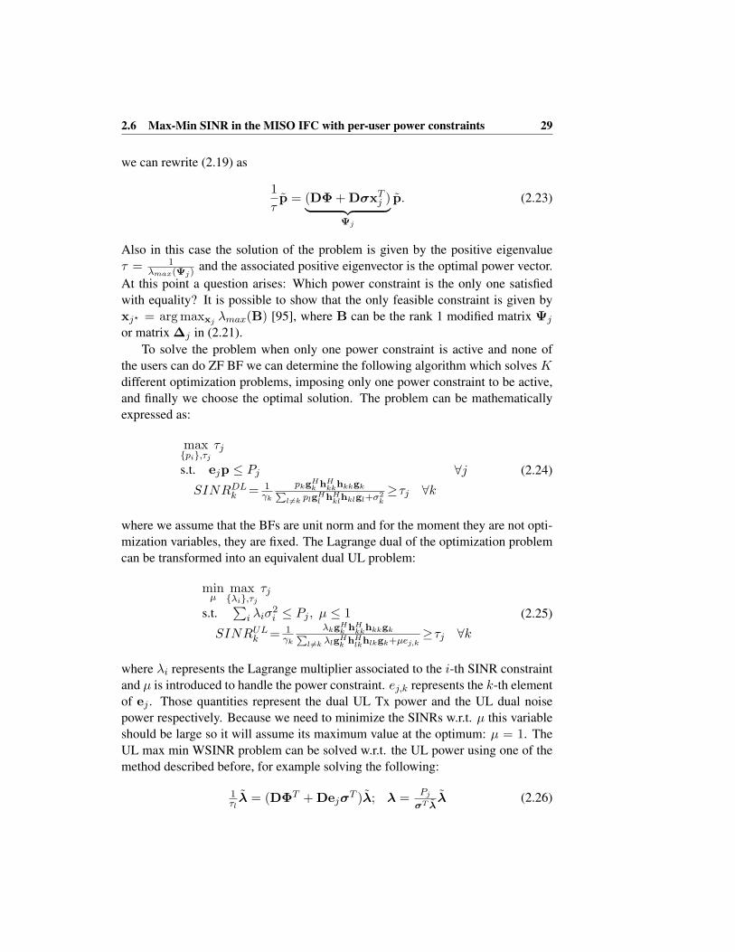
2.6 Max-Min SINR in the MISO IFC with per-user power constraints 29
we can rewrite (2.19) as
1
τp = (DΦ+DσxT
j )︸ ︷︷ ︸Ψj
p. (2.23)
Also in this case the solution of the problem is given by the positive eigenvalue
τ = 1λmax(Ψj)
and the associated positive eigenvector is the optimal power vector.
At this point a question arises: Which power constraint is the only one satisfied
with equality? It is possible to show that the only feasible constraint is given by
xj⋆ = argmaxxj λmax(B) [95], where B can be the rank 1 modified matrix Ψj
or matrix ∆j in (2.21).
To solve the problem when only one power constraint is active and none of
the users can do ZF BF we can determine the following algorithm which solves Kdifferent optimization problems, imposing only one power constraint to be active,
and finally we choose the optimal solution. The problem can be mathematically
expressed as:
max{pi},τj
τj
s.t. ejp ≤ Pj
SINRDLk = 1
γk
pkgHk hH
kkhkkgk∑l 6=k plg
Hl hH
klhklgl+σ2k
≥τj ∀k∀j (2.24)
where we assume that the BFs are unit norm and for the moment they are not opti-
mization variables, they are fixed. The Lagrange dual of the optimization problem
can be transformed into an equivalent dual UL problem:
minµ
max{λi},τj
τj
s.t.∑
i λiσ2i ≤ Pj , µ ≤ 1
SINRULk = 1
γk
λkgHk hH
kkhkkgk∑l 6=k λlg
Hk hH
lkhlkgk+µej,k≥τj ∀k
(2.25)
where λi represents the Lagrange multiplier associated to the i-th SINR constraint
and µ is introduced to handle the power constraint. ej,k represents the k-th element
of ej . Those quantities represent the dual UL Tx power and the UL dual noise
power respectively. Because we need to minimize the SINRs w.r.t. µ this variable
should be large so it will assume its maximum value at the optimum: µ = 1. The
UL max min WSINR problem can be solved w.r.t. the UL power using one of the
method described before, for example solving the following:
1τlλ = (DΦT +Dejσ
T )λ; λ =Pj
σT λλ (2.26)
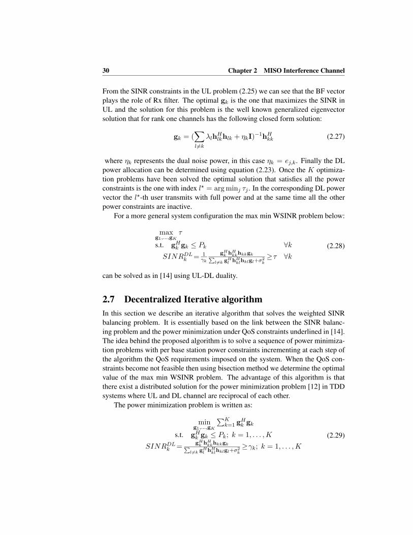
30 Chapter 2 MISO Interference Channel
From the SINR constraints in the UL problem (2.25) we can see that the BF vector
plays the role of Rx filter. The optimal gk is the one that maximizes the SINR in
UL and the solution for this problem is the well known generalized eigenvector
solution that for rank one channels has the following closed form solution:
gk = (∑
l 6=k
λlhHlkhlk + ηkI)
−1hHkk (2.27)
where ηk represents the dual noise power, in this case ηk = ej,k. Finally the DL
power allocation can be determined using equation (2.23). Once the K optimiza-
tion problems have been solved the optimal solution that satisfies all the power
constraints is the one with index l⋆ = argminj τj . In the corresponding DL power
vector the l⋆-th user transmits with full power and at the same time all the other
power constraints are inactive.
For a more general system configuration the max min WSINR problem below:
maxg1,...,gK
τ
s.t. gHk gk ≤ Pk ∀k
SINRDLk = 1
γk
gHk hH
kkhkkgk∑l 6=k gH
l hHklhklgl+σ2
k
≥τ ∀k(2.28)
can be solved as in [14] using UL-DL duality.
2.7 Decentralized Iterative algorithm
In this section we describe an iterative algorithm that solves the weighted SINR
balancing problem. It is essentially based on the link between the SINR balanc-
ing problem and the power minimization under QoS constraints underlined in [14].
The idea behind the proposed algorithm is to solve a sequence of power minimiza-
tion problems with per base station power constraints incrementing at each step of
the algorithm the QoS requirements imposed on the system. When the QoS con-
straints become not feasible then using bisection method we determine the optimal
value of the max min WSINR problem. The advantage of this algorithm is that
there exist a distributed solution for the power minimization problem [12] in TDD
systems where UL and DL channel are reciprocal of each other.
The power minimization problem is written as:
ming1,...,gK
∑Kk=1 g
Hk gk
s.t. gHk gk ≤ Pk; k = 1, . . . ,K
SINRDLk =
gHk hH
kkhkkgk∑l 6=k gH
l hHklhklgl+σ2
k
≥γk; k = 1, . . . ,K
(2.29)
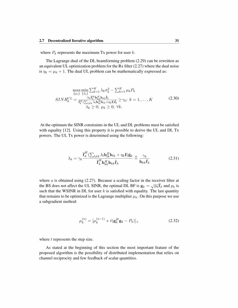
2.7 Decentralized Iterative algorithm 31
where Pk represents the maximum Tx power for user k.
The Lagrange dual of the DL beamforming problem (2.29) can be rewritten as
an equivalent UL optimization problem for the Rx filter (2.27) where the dual noise
is ηk = µk + 1. The dual UL problem can be mathematically expressed as:
max{µi}
min{λi}
∑Kk=1 λkσ
2k −
∑Kk=1 µkPk
SINRULk =
λk fHk hH
kkhkk fk
fHk (∑
l 6=k λlhHlkhlk+ηkI)fk
≥γk; k = 1, . . . ,K
λk ≥ 0; µk ≥ 0; ∀k.
(2.30)
At the optimum the SINR constraints in the UL and DL problems must be satisfied
with equality [12]. Using this property it is possible to derive the UL and DL Tx
powers. The UL Tx power is determined using the following:
λk = γkfHk (∑
l 6=k λlhHlkhlk + ηkI)gk
fHk hH
kkhkkfk
a=
γk
hkkfk(2.31)
where a is obtained using (2.27). Because a scaling factor in the receiver filter at
the BS does not affect the UL SINR, the optimal DL BF is gk =√pkfk and pk is
such that the WSINR in DL for user k is satisfied with equality. The last quantity
that remains to be optimized is the Lagrange multiplier µk. On this purpose we use
a subgradient method:
µ(n)k = [µ
(n−1)k + t(gH
k gk − Pk)]+ (2.32)
where t represents the step size.
As stated at the beginning of this section the most important feature of the
proposed algorithm is the possibility of distributed implementation that relies on
channel reciprocity and few feedback of scalar quantities.

32 Chapter 2 MISO Interference Channel
Algorithm 1 Iterative Algorithm for max min WSINR
Initialize: i= 0 and a feasible γ0 = [γ(0)1 , . . . , γ
(0)K ]
repeat
i=i+1
Find g(i)k solving Power min for γ(i)
Set γmin = γ(i)
Increase γ(i+1) = αγ(i)
until γ(i) is feasible
repeat
Set γmax = γ(i)
i=i+1
Set γ(i) = γmax+γmin
2
Find g(i)k solving Power min for γ(i)
if γ(i) is feasible then
Set γmin = γ(i)
else
Set γmax = γ(i)
end if
until |γmax − γmin| < ǫ
2.8 SINR Region Characterization
The beamforming problem in terms of max min WSINR described in (2.18) and
further refined in (2.28) can be interpreted as exploring the SINR region along the
ray with direction γ = [γ1, . . . , γK ]. Solving the max min WSINR problem allows
us to find the maximum values of SINR on the direction given by γ. Then the op-
timal point is given by the intersection of the straight line described by γ and the
Pareto boundary of the SINR region. This result was claimed for a SISO IFC in
[89] and in [20] for the two user MISO IFC, here is extended to the more general
K-user MISO case. The Pareto boundary of the SINR region is commonly defined
as follows:
A SINR tuple (S1, . . . , SK) belongs to the Pareto boundary if there is no other tuple
(S1, . . . , SK) with (S1, . . . , SK) ≥ (S1, . . . , SK) and (S1, . . . , SK) 6= (S1, . . . , SK).This result is important from an information theoretic point of view because solving
the simple max min WSINR problem allows us to draw the entire Pareto boundary
of the rate region, thanks to the logarithmic relation between SINRs and rates. This
result is valid for a general K-user MISO IFC regardless of system parameters. In
a recent paper [19] the authors provide a characterization of the Pareto boundary

2.9 Numerical Examples 33
of the Rate region where the BF at each base station is a linear combination of the
cross channels directly connected to it. This representation requires K(K − 1)complex parameters while the use of max min WSINR only requires (K − 1) real
values, the fairness constraints γk. In [21] the authors propose a similar character-
ization of the Pareto boundary of the rate region using what they call rate profile.
That problem can be thought as a rate balancing problem imposing different pri-
ority constraints and they state that to solve the problem a centralized solution is
necessary.
On the other hand for max min WSINR it is possible to develop a distributed al-
gorithm to solve the problem, as shown in the previous section, that represents a
preferable solution compares to a centralized approach. In a recent paper [22] a
similar result has been introduced. The authors study the Pareto characterization
for a multicell DL system, where the IFC is a special case, introducing also hard-
ware impairments. The solution proposed requires the same number of parameters,
compare to the one proposed here, for the complete characterization of the Pareto
boundary.
2.9 Numerical Examples
In this section we present some numerical results in which we study the behavior
of the proposed algorithm to solve the max min WSINR. In Fig. 2.3 we report the
Rate region of a 2-user MISO IFC where each base station has Mk = 2, ∀k trans-
mitting antennas for a single channel realization. We plot on the same figure the
rate obtained optimizing the max min WSINR for different priority constraints
γk. The rate region reported, the region in the figures represented with the blue
markers, is obtained using the BF parametrization proposed in [19] for the 2-user
MISO IFC that allows to draw the entire rate region, and hence also the Pareto
boundary. As we can see the rates obtained optimizing the max min WSINR (red
Figure 2.3: Rate region for a 2-user MISO IFC for σ2k = 30 dB
points in the figure) lie always on the boundary of the region. In addition we can
see that varying the priority constraint γk it is possible to explore different points
on the boundary. This figure sustain our statement on the possibility to charac-
terize the entire Pareto boundary of the rate region using max min WSINR. The
solid lines drawn on the figure represent the rays with direction given by γ. Those
curves are straight lines in the SINR region, Fig. 2.4, but due to the log relation
between SINR and Rate they have a logarithmic behavior.
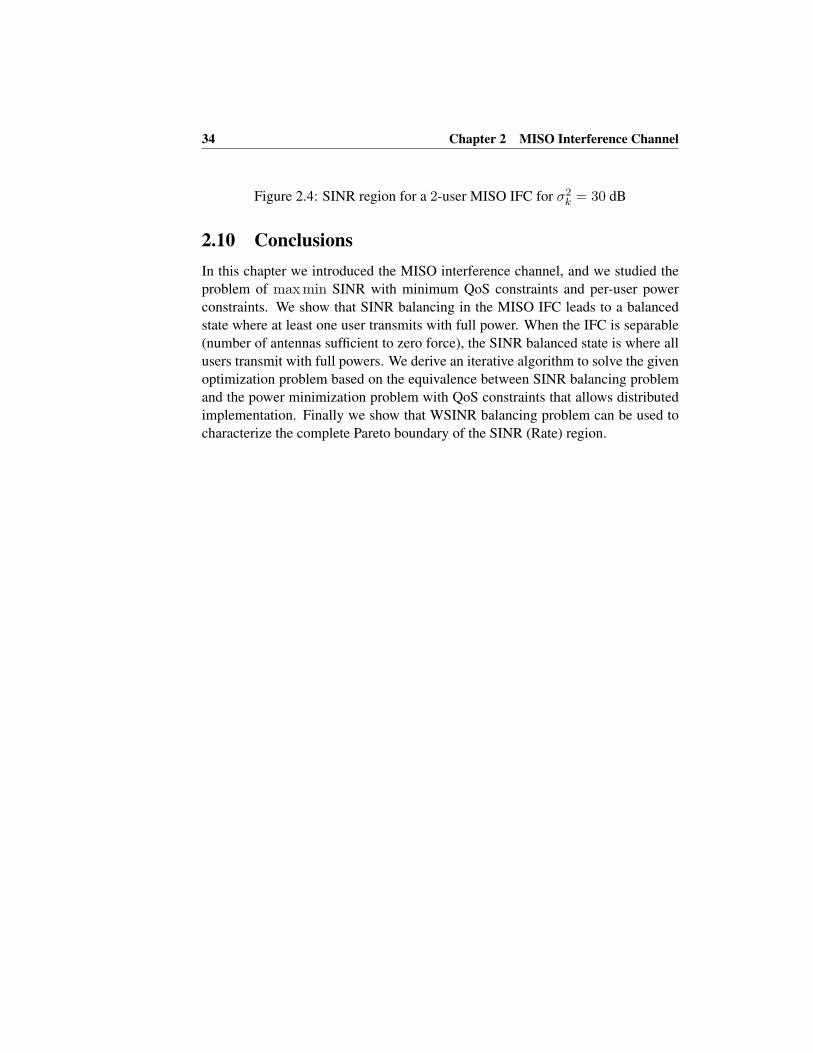
34 Chapter 2 MISO Interference Channel
Figure 2.4: SINR region for a 2-user MISO IFC for σ2k = 30 dB
2.10 Conclusions
In this chapter we introduced the MISO interference channel, and we studied the
problem of maxmin SINR with minimum QoS constraints and per-user power
constraints. We show that SINR balancing in the MISO IFC leads to a balanced
state where at least one user transmits with full power. When the IFC is separable
(number of antennas sufficient to zero force), the SINR balanced state is where all
users transmit with full powers. We derive an iterative algorithm to solve the given
optimization problem based on the equivalence between SINR balancing problem
and the power minimization problem with QoS constraints that allows distributed
implementation. Finally we show that WSINR balancing problem can be used to
characterize the complete Pareto boundary of the SINR (Rate) region.

Chapter 3
Interference Alignment
Feasibility for MIMO
Interference Channel
3.1 Introduction and state of art
The capacity of an interference channel in general has been an open problem
for long time. The best known result is given for the 2-users SISO Gaussian
IFC in [8], for K > 2 the problem becomes even more complicated. This has
lead to an alternative line of attack; that of characterizing the capacity region
in terms of sum-capacity pre-log factor, the so called total degrees of freedom
(DoF), that gives a good approximation of the sum capacity at high SNR. A first
study on the DoF for a MIMO IFC has been done in [25] where the DoF for
a 2-user MIMO IFC has been found. There it has been shown that for a sys-
tem with M1,M2 transmitting antennas and N1, N2 receiving antennas a total
d = min{M1 + M2, N1 + N2,max{M1, N2},max{M2, N1}} interference free
streams can be achieved if perfect channel state information is available at both
transmitters and receivers. For system with more users a different approach is nec-
essary. In [26] the concept of interference alignment (IA) has been introduced,
then in [27] the same concept has been applied to the MIMO X channel where the
authors showed that an higher total DoF can be achieved compared to previously
known results. Then in the recent paper [28] the authors have demonstrated the
35

36 Chapter 3 Interference Alignment Feasibility for MIMO Interference Channel
achievability of a capacity prelog factor of K/2 in a K-user interference channel.
This result has been achieved for time-varying channel where the alignment is ob-
tained using infinite symbol extensions. In addition they also give an example on
how to apply IA in constant coefficient MIMO IFC where the preliminary result
of 3M2 total DoF for a K = 3 users constant coefficient MIMO IFC is determined.
This result can be generalized for time-varying channel to KM2 . These remark-
able results are achieved using simple linear transmit-receiver filters. This has
resulted in a renewed interest in joint linear processing at transmitter and receiver
with the aim of maximizing the capacity prelog of a multiuser MIMO interference
channel. In particular IA exploits the availability of channel state information at
the transmitter (CSIT) to compute appropriate beamforming matrices such that,
at each receiver, all the interference is confined within a subspace of dimension
complementary to the receiver’s desired signal subspace dimension. Thus, simple
zero-forcing (ZF) receivers are enough to separate the desired signal from the in-
terferers. The alignment of the interference contributions can be done in different
ways. IA over the signal scale encodes the transmitted signal, using for examples
lattice codes, such that the alignment is done at the signal level [96],[97]. On the
other hand alignment over the signal space takes advantages of aligning the inter-
ferers along different transmits directions [28] like space, time or frequency. In
[98] it has been shown that a DoF of K2 can be achieved almost surely in a K-user
real IFC with constant coefficients. This can be achieved using a new alignment
scheme, called real alignment, based on proprieties of rational and irrational num-
bers. New achievable DoF for K-users symmetric M × N MIMO IFC has been
introduced in [29]. In particular a total number of DoF of Kmin(M,N) if K ≤ R,
and for K > R it is upper-bounded bymax{M,N}
R+1 , with R =⌊max{M,N}min{M,N}
⌋, for both
constant or time varying channels. For only time varying channel coefficients they
have shown that RR+1 min{M,N} total DoF can be achieved. Similar results have
been extended to constant channels in [30] where the method proposed in [98] is
extended to the MIMO case.
While it is known that interference alignment is the optimal scheme (in the
high SNR regime) among approaches that use linear transmit/receive processing
and treat interference as Gaussian noise, the existence of solutions in many cases is
not known in general. In [31] a close form IA solution is provided for square sym-
metric K-user MIMO IFC where each pair of users is equipped with N = K − 1antennas and wants to transmit one stream each. The same solution has been ex-
tended to the case of d transmitted streams in [32]. Iterative algorithms, for finding
numerically an IA solution have been proposed [33, 34, 35, 36], they can be also
used to evaluate the existence of an IA solution through simulations. To achieve
IA different approaches are used. In [33] [34] the interference leakage at each

3.1 Introduction and state of art 37
receiver is minimized, the authors of [35] introduce an algorithm that solves a least
squares problem in an iterative fashion. [36] explores the minimization of the mean
squared error (MSE) as cost function for the IA problem in MIMO IFC. The fea-
sibility of IA solutions for a constant coefficient MIMO IFC was studied in [37].
There, when dk = 1 ∀k, a MIMO IFC with a given distribution of Tx/Rx antennas
is classified as proper or improper. All proper systems are almost surely (a.s) fea-
sible. For a system to be proper, it is required that, for every subset of equations
that arise due to the IA constraints, the number of variables be at least equal to the
number of equations in that subset. This condition (that the system be proper) is
sufficient but may not be necessary. Moreover, such a classification can be compu-
tationally expensive even for systems with relatively small number of transmit and
receive antennas. Furthermore, for an arbitrary DoF allocation amongst users (dknot constrained to be 1), additional outerbounds need to be satisfied for a system to
be feasible. It turns out however, that for multi-stream transmission, conformance
with the outerbounds do not necessarily provide insight into the feasibility of an
IA solution. In other words, an IA solution is not guaranteed if the outerbounds are
satisfied. An example follows: For a K = 3 user MIMO IFC where dk = 2 ∀k,
M1 = N1 = 4, M2 = 5, N2 = 3, and M3 = 6, N3 = 2, the outerbounds (cf. (21)
in [37]) are satisfied. However, the system does not admit an IA solution.
Similar approach of [37] was proposed in [99] to study feasibility of IA for a DL
multiuser cellular network. In [38] the approach of counting the number of vari-
ables and the number of constraints in the IA problem has been studied under the
more rigorous approach of algebraic geometry. The authors showed that the given
approach represents a necessary and sufficient condition for the square symmet-
ric MIMO IFC, i.e. equal number of transmit and receive antennas at all users.
In a more recent paper [39] the same authors of [38] introduced a new feasibil-
ity study founding a condition that is both necessary and sufficient for a K = 3user MIMO symmetric IFC with M transmitting and N receiving antennas at all
terminals, each of them wants to transmit d streams. Another implication of their
study is that the feasibility conditions based on comparing number variables and
constraints does not always predict feasibility for the particular symmetric MIMO
IFC under consideration. In a recent paper [100] has been shown that studying
the feasibility problem for a given set of channel matrices is an NP-hard problem.
On the other hand the problem studied in this chapter and in the other papers pre-
sented in this section consider feasibility for a general set of channel matrices with
given dimensions, this problem is easier to be solved [101]. In [101] the authors
studied the problem of IA feasibility for a general K-users IFC using results from
algebraic geometry and differential topology. In [102, 103, 104, 105] IA for Par-
tially connected channels has been studied. These networks are characterized by
the propriety that some of the interfering links have zero gain, so each communi-
38 Chapter 3 Interference Alignment Feasibility for MIMO Interference Channel
cation interferes only with a subset of user pairs. [104] studies the case of K-user
MIMO IFC, where the model can be used to study arbitrary large networks, also
feasibility conditions, based on the results in [37], for this particular interference
channel are given. Then the results are applied to a more realistic cellular system
model in [103].
3.2 Contributions
In this chapter we first introduce the system model of a K-user MIMO IFC that
will also be used in the following chapters. Then we propose a systematic method
to check feasibility of IA solutions for a given K-link Noisy MIMO IFC and an
arbitrary DoF allocation. In particular, starting from interference alignment con-
straints, we introduce a recursive algorithm that allows an analytical evaluation of
the existence of IA solutions (or lack thereof) for a given degrees of freedom al-
location. We introduce a set of necessary conditions that if not satisfied prevents
the existence of an interference alignment solution. Our approach is then validated
using some numerical examples, comparing the result of our feasibility check with
the convergence propriety of an iterative algorithm for determining IA solutions
[34]. In addition we discuss interference alignment duality and we introduce the
interpretation of IA as a constraint compressed SVD. Then an alternative IA fea-
sibility check is introduced based on the idea that a stream can be suppressed at
either the transmit or at the receive side. This suggestion is supported by the in-
troduction of Homotopy method for IA. Finally we introduce the observation that
working with real constellation, transmitted over complex channel, can be inter-
preted as transmission over real channel with doubled dimensions. This allows to
increase the granularity for a finer adjustment of the achievable DoF.
3.3 System Model
Figure 3.1: MIMO Interference channel
Fig. 7.2 depicts a K-link MIMO interference channel with K transmitter-
receiver pairs. To differentiate the two transmitting and receiving devices we as-
sume that each of the K pairs is composed of a Base station (BS) and a Mobile user
(MU). This is only for notational purposes. The k-th BS and its corresponding MU
are equipped with Mk and Nk antennas respectively. The k-th transmitter gener-
ates interference at all l 6= k receivers. The received signal in the Downlink (DL)
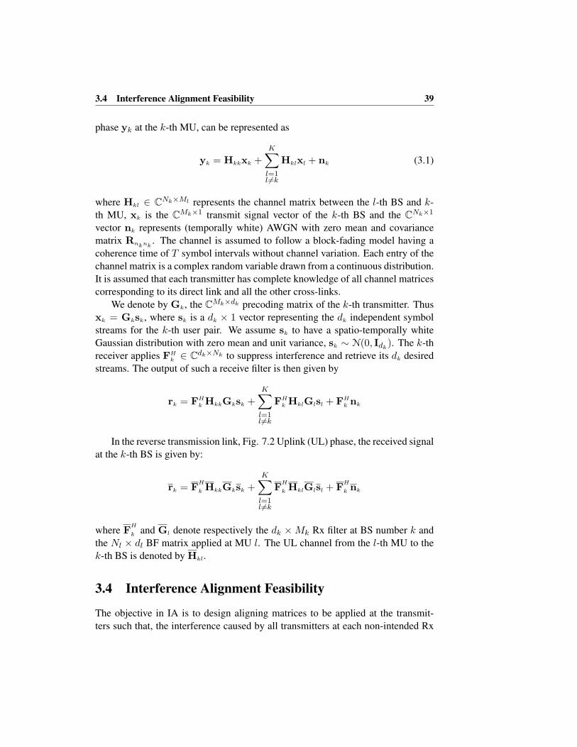
3.4 Interference Alignment Feasibility 39
phase yk at the k-th MU, can be represented as
yk = Hkkxk +
K∑
l=1l 6=k
Hklxl + nk (3.1)
where Hkl ∈ CNk×Ml represents the channel matrix between the l-th BS and k-
th MU, xk is the CMk×1 transmit signal vector of the k-th BS and the CNk×1
vector nk represents (temporally white) AWGN with zero mean and covariance
matrix Rnknk. The channel is assumed to follow a block-fading model having a
coherence time of T symbol intervals without channel variation. Each entry of the
channel matrix is a complex random variable drawn from a continuous distribution.
It is assumed that each transmitter has complete knowledge of all channel matrices
corresponding to its direct link and all the other cross-links.
We denote by Gk, the CMk×dk precoding matrix of the k-th transmitter. Thus
xk = Gksk, where sk is a dk × 1 vector representing the dk independent symbol
streams for the k-th user pair. We assume sk to have a spatio-temporally white
Gaussian distribution with zero mean and unit variance, sk ∼ N(0, Idk). The k-th
receiver applies FHk ∈ Cdk×Nk to suppress interference and retrieve its dk desired
streams. The output of such a receive filter is then given by
rk = FHk HkkGksk +
K∑
l=1l 6=k
FHk HklGlsl + FH
k nk
In the reverse transmission link, Fig. 7.2 Uplink (UL) phase, the received signal
at the k-th BS is given by:
rk = FH
k HkkGksk +
K∑
l=1l 6=k
FH
k HklGlsl + FH
k nk
where FH
k and Gl denote respectively the dk × Mk Rx filter at BS number k and
the Nl × dl BF matrix applied at MU l. The UL channel from the l-th MU to the
k-th BS is denoted by Hkl.
3.4 Interference Alignment Feasibility
The objective in IA is to design aligning matrices to be applied at the transmit-
ters such that, the interference caused by all transmitters at each non-intended Rx
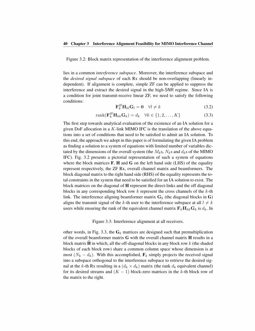
40 Chapter 3 Interference Alignment Feasibility for MIMO Interference Channel
Figure 3.2: Block matrix representation of the interference alignment problem.
lies in a common interference subspace. Moreover, the interference subspace and
the desired signal subspace of each Rx should be non-overlapping (linearly in-
dependent). If alignment is complete, simple ZF can be applied to suppress the
interference and extract the desired signal in the high-SNR regime. Since IA is
a condition for joint transmit-receive linear ZF, we need to satisfy the following
conditions:
FHk HklGl = 0 ∀l 6= k (3.2)
rank(FHk HkkGk) = dk ∀k ∈ {1, 2, . . . ,K} (3.3)
The first step towards analytical evaluation of the existence of an IA solution for a
given DoF allocation in a K-link MIMO IFC is the translation of the above equa-
tions into a set of conditions that need to be satisfied to admit an IA solution. To
this end, the approach we adopt in this paper is of formulating the given IA problem
as finding a solution to a system of equations with limited number of variables dic-
tated by the dimensions of the overall system (the Mks, Nks and dks of the MIMO
IFC). Fig. 3.2 presents a pictorial representation of such a system of equations
where the block matrices F, H and G on the left hand side (LHS) of the equality
represent respectively, the ZF Rx, overall channel matrix and beamformers. The
block diagonal matrix to the right hand side (RHS) of the equality represents the to-
tal constraints in the system that need to be satisfied for an IA solution to exist. The
block matrices on the diagonal of H represent the direct-links and the off diagonal
blocks in any corresponding block row k represent the cross channels of the k-th
link. The interference aligning beamformer matrix Gk (the diagonal blocks in G)
aligns the transmit signal of the k-th user to the interference subspace at all l 6= kusers while ensuring the rank of the equivalent channel matrix FkHkkGk is dk. In
Figure 3.3: Interference alignment at all receivers.
other words, in Fig. 3.3, the Gk matrices are designed such that premultiplication
of the overall beamformer matrix G with the overall channel matrix H results in a
block matrix H in which, all the off-diagonal blocks in any block row k (the shaded
blocks of each block row) share a common column space whose dimension is at
most (Nk − dk). With this accomplished, Fk simply projects the received signal
into a subspace orthogonal to the interference subspace to retrieve the desired sig-
nal at the k-th Rx resulting in a (dk × dk) matrix (the rank dk equivalent channel)
for its desired streams and (K − 1) block-zero matrices in the k-th block row of
the matrix to the right.

3.4 Interference Alignment Feasibility 41
The only requirement on the (dk × dk) matrix that mixes up the desired streams
is that it be of full rank. The beamforming matrix therefore, is determined up to
an arbitrary (dk × dk) square matrix. Thus, of the total number of (Mk × dk)variables available for the design of Gk matrix, transmission of dk independent
streams results in an immediate loss of d2k variables thus reducing the total number
of variables available for the design of an interference aligning beamformer at each
Tx to dk(Mk − dk). The reason for evaluating the number of variables available
at the Tx is the nature of the IA problem. The IA scheme essentially requires that
all alignment is done at the Tx. Therefore every Tx imposes a set of constraints on
the entire system (as a consequence of alignment conditions at each non intended
Rx) whenever it transmits a stream to its Rx. Thus, an IA solution will be feasi-
ble only if the total number of variables available in the system is greater than or
equal to the total number of constraints to be satisfied. Moreover, the variables
should be distributed appropriately at each of the Tx. In the sequel, we provide
a systematic method of counting the number of variables available for the design
of an interference aligning beamformer at each Tx and comparing them with the
constraints imposed on the system by each Tx. This method can be seen as arriv-
ing at the K-link MIMO IFC for which the existence of an IA solution is to be
analyzed, by successively adding a single Tx and computing the total number of
variables available for the joint design of the interference aligning beamformers at
the transmitters and comparing it against the total number of alignment constraints
imposed by the Tx (due to its dk streams) at each step of this build-up.
The main idea of our approach is to convert the alignment requirements at each Rx
into a rank condition of an associated interference matrix. At Rx k, the interference
due to all other (K − 1) transmitters is grouped into a (Nk ×∑K
l=1;l 6=k dl) matrix
H[k]I =[Hk1G1, ...Hk(k−1)G(k−1),Hk(k+1)G(k+1), ...HkkGK ],
that spans the interference subspace at the k-th Rx. We call this the interference
matrix at user k. The total signal-space dimension at Rx k is given by the total
number of receive antennas Nk, of which dk interference-free signaling dimen-
sions are to be reserved for the signal from the k-th Tx. This is achieved when
the interference from all other transmitters lies in an independent subspace whose
dimension can be at most (Nk − dk). Thus the dimension of the subspace spanned
by the matrix H[k]I must satisfy
rank(H[k]I ) = r[k]
I ≤ Nk − dk (3.4)
While the above equation prescribes an upperbound for the rank of the interference
matrix, the nature of the channel matrix (full rank property) combined with the

42 Chapter 3 Interference Alignment Feasibility for MIMO Interference Channel
rank requirement of the beamformer at each Tx (rank(Gk) = dk) specifies the
following lower bound on r[k]I
r[k]I ≥ max
l 6=k(dl − [Ml −Nk]+) (3.5)
In the bound above we considered a pairwise communication where the k-th user
receives interference by only one transmitter, [x]+ = max(0, x) and [Ml − Nk]+discounts the possibility of the columns of Gl belonging to the orthogonal com-
plement of Hkl. Forcing the rank of n × m matrix A to some r ≤ min(m,n)implies imposing (n − r)(m − r) constraints. We explain this briefly as follows.
Without loss of generality, (w.l.o.g) assume that the columns of this n×m matrix
are partitioned into A = [A1;A2] where A1 is n × r and is of full column rank.
Then imposing a rank r on A implies that A2 shares the same column space as A1
which in turn implies that A⊥T1 A2 = 0. Since A⊥
1 is n × (n − r), it follows that
(n−r)(m−r) constraints need to be satisfied for A to be of rank r. Thus imposing
a rank r[k]I on H
[k]I implies imposing
(Nk − r[k]I )(
K∑
l=1l 6=k
dl − r[k]I )
constraints at Rx k. r[k]I is maximum when the interference contribution of each
interferer spans an independent subspace. Which leads us to the upper bound r[k]I ≤∑K
l=1;l 6=k dl. However, accounting for the inequality in (3.4) we have
r[k]I ≤ min(dtot, Nk)− dk (3.6)
where dtot =∑K
k=1 dk, and min(.) operation appears in the above equation due to
the fact that the rank of H[k]I cannot exceed its dimensions.
3.5 Recursive procedure to evaluate feasibility
In this section we detail a recursive method of evaluating the feasibility of an IA
solution for a MIMO IFC and a corresponding DoF distribution. As mentioned
earlier, the main idea here is to interpret the interference alignment requirement
at each Rx as forcing a certain rank on the associated interference channel H[k]I
which in turn imposes a certain number of constraints on the IA problem. In the
earlier section we show that this rank is bounded above and below by the system
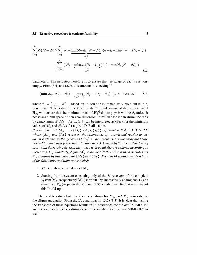
3.5 Recursive procedure to evaluate feasibility 43
k∑
i=1
di(Mi−di)≥k∑
i=1
(Ni−min(d−di, (Ni−di))︸ ︷︷ ︸r[i]I
)(d−di−min(d−di, (Ni−di)))
+
K∑
i=k+1
( Ni −min(d, (Ni − di))︸ ︷︷ ︸r[i]I
)( d−min(d, (Ni − di)) )
(3.8)
parameters. The first step therefore is to ensure that the range of each ri is non-
empty. From (3.4) and (3.5), this amounts to checking if
(min(dtot, Nk)− dk)− maxj∈K−{k}
(dj − [Mj −Nk]+) ≥ 0 ∀k ∈ K (3.7)
where K = {1, 2, ...K}. Indeed, an IA solution is immediately ruled out if (3.7)
is not true. This is due to the fact that the full rank nature of the cross channel
Hkj will ensure that the minimum rank of H[k]I due to j 6= k will be dj unless it
possesses a null space of non zero dimension in which case it can shrink the rank
by a maximum of [Mj −Nk]+. (3.7) can be interpreted as check for the minimum
values of Mk and Nk ∀k for a given DoF allocation.
Proposition: Let MK = {{Mk}, {Nk}, {dk}} represent a K-link MIMO IFC
where {Mk} and {Nk} represent the ordered set of transmit and receive anten-
nas of each user in the system and {dk} is the ordered set of the associated DoF
desired for each user (ordering is by user index). Denote by Ko the ordered set of
users with decreasing dk such that users with equal dks are ordered according to
increasing Mk. Similarly, define M′
K to be the MIMO IFC and the associated set
K′
o obtained by interchanging {Mk} and {Nk}. Then an IA solution exists if both
of the following conditions are satisfied:
1. (3.7) holds true for MK and M′
K
2. Starting from a system consisting only of the K receivers, if the complete
system MK (respectively M′
K) is “built” by successively adding one Tx at a
time from Ko (respectively K′
o) and (3.8) is valid (satisfied) at each step of
this “build-up”.
The need to satisfy both the above conditions for MK and M′
K arises due to
the alignment duality. From the IA conditions in (3.2) (3.3), it is clear that taking
the transpose of these equations results in IA conditions for the dual MIMO IFC
and the same existence conditions should be satisfied for this dual MIMO IFC as
well.

44 Chapter 3 Interference Alignment Feasibility for MIMO Interference Channel
At each step k of the recursion, (3.8) accumulates the total number of variables
available for designing an IA solution in an associated sub-problem comprising of
a k-link MIMO IFC where only k transmitters are transmitting non-zero streams
and aligning their streams into some interference subspace of all non-intended re-
ceivers in the LHS of (3.8). The RHS accumulates the total number of constraints
at all receivers that arise due to these transmitters. That the number of variables
contributed by the i-th Tx is given by di(Mi−di) is obvious from the discussion in
the previous section. We now elaborate on the method of obtaining the constraints
on the RHS of (3.8). Forcing a rank on H[k]I amounts to satisfying a number of
constraints that is a function of the rank and the dimensions of H[k]I . While we do
not have knowledge of the exact rank of H[k]I at each k (since that will be the result
of the IA design whose feasibility we are evaluating in the first place) we do know
the numerical range of r[k]I for each k. Therefore, instead of using the actual rank it
is useful to use its upperbound (denoted by r[k]I , as specified in (3.6)). On the RHS
of (3.8) the first summation reflects the total number of constraints to be satisfied
for an IA solution to exist in a k-link MIMO IFC with k-links transmitting a total
of d =k∑
i=1
di streams. For each user i accounted for in this summation, we have
to ensure that at Rx-i, r[i]I ≤ (Ni − di). The column dimension of H
[i]I is (d− di).
In order to minimize the total number of constraints that we impose of the system
(due to the act of forcing a particular r[i]I at the i-th Rx), we choose the maximum
possible rank of r[i]I , which we know to be min(column dimensions, Ni − di) i.e.,
r[i]I = min(d − di, Ni − di). The second summation consists of all “un-paired”
receivers in the sub-problem i.e., those receivers whose corresponding transmitters
are presently not transmitting any streams but still need d streams to be aligned in
their interference subspace. Therefore, the maximum allowable rank of the inter-
ference matrices for all these receivers is r[i]I = min(d,Ni − di). Thus, (3.8) when
true at each step, verifies that the number of variables available for the design of
IA beamformers at all k transmitters is greater than the number of constraints that
are imposed by an IA solution. In fact, it verifies that its is possible to align all the
interference not just in the associated k-link MIMO IFC but also in the interference
subspace of all un-intended receivers that are not in the k-link MIMO IFC (the un-
paired receivers accounted for in the second summation). Finally, the ordering of
the users in terms of increasing dk in Ko (K′
o for M′
K) ensures early identification
of in-feasibility of an IA solution since a larger DoF requirement typically results
in smaller number of variables available at the Tx in order to meet the rank con-
straints.
In the next section we present numerical examples to show that our approach is
able to check the feasibility (or in-feasibility) of an IA solution for a given MIMO

3.6 Numerical Examples 45
IFC. For a MK which conforms to both the conditions of our approach, we are
able cross validate that an IA solution exists using an iterative algorithm proposed
in [34]. Indeed, it can be shown that the algorithm in [34] will always converge
to an optimum solution when our conditions are met since convergence to an op-
timum solution implies that the dk minimum eigenvalues of∑
i 6=k HkiGiGHi HH
ki
are zero which will be true if rank(H[k]I ) ≤ min(dtot, Nk)− dk which is a part by
our systematic approach.
3.6 Numerical Examples
In this section we provide some numerical examples to validate the conditions de-
rived in this paper. In all the examples given in this section, when the MIMO IFC
that satisfied the conditions in Sec. 3.5, the numerical algorithm in [34] was able
to find an IA solution whereas it failed to find one when these conditions were not
satisfied. We tested our conditions extensively with varied antenna and stream dis-
tributions. In particular, all the examples in [37] we also tested.
Example 1: Consider a 2-link MIMO system with M = 2, N = 4, d = 2. This
system satisfies the 2 conditions in Sec. 3.5 and IA solutions do exist for this sys-
tem.
Example 2: Similarly, the 6 user case where Mk = 3, Nk = 4, dk = 1∀k, both
conditions in Sec. 3.5 are satisfied and an IA solution is possible for this case.
Example 3: We now look at another 2-link MIMO system with M1 = 4, N1 =7, d1 = 3,M2 = 10, N2 = 4, d2 = 2. For this system, the rank conditions are not
satisfied and indeed, there is no IA solution for this case.
Example 4: In the 4-link case characterized by Mk = 2, Nk = 3 k = 1, 2, 3 and
M4 = N4 = 2 dk = 1∀k. The rank conditions are satisfied but (3.8) is not satis-
fied. Therefore we conclude that there cannot be an interference alignment solution
for this system.
3.7 Alignment Duality
There are another set of conditions that need to be considered in order to complete
the existence conditions. These conditions arise from the equations
FHl HlkGk = 0 ∀k 6= l (3.9)
rank(FHk HkkGk) = dk ∀k ∈ {1, 2, . . . ,K} (3.10)
which corresponds to the interference alignment constraints of the dual problem
where all transmitters and receivers exchange roles. In other words, when Fl =

46 Chapter 3 Interference Alignment Feasibility for MIMO Interference Channel
GHl ,Gk = FH
k ,Hlk = HHkl in (3.9) and (3.10). The dual problem of an inter-
ference channel is again an interference channel, involving the reciprocal channel.
For the ZF case (interference alignment) the conditions (3.9)-(3.10) for the dual
problem are obtained immediately by simply taking the transpose of (3.2)-(3.3) for
the original problem [33]. If the ZF filters are replaced by MMSE receive filters
that are the optimal interference suppressing filters (c.f. Sec.4.4.1) we conjecture
a sum-rate duality for the K-user MIMO interference channel for an appropriate
choice of receiver noise covariance matrices and transmit power constraints. This
duality for maximizing the sum rate will be analyzed in more detail in this thesis in
chapter 4. In this section we focus on interference alignment duality and hence re-
strict ourselves to a ZF design. As a direct consequence of interference alignment
duality, for an interference alignment solution to exist, the conditions in (3.7)- (3.8)
should also be satisfied when the Mk and Nk are interchanged.
3.8 IA as a Constrained Compressed SVD
For IA purposes, the FHk , Gi can be constrained to be (column) unitary, since only
their column spaces matter. As a result, the matrices FH , G below are (column)
unitary (FFH = I,GHG = I). Now, it is useful to think of an IA solution as a
constrained compressed SVD in the following form:
FHHG =
FH1 0 · · · 0
0 FH2
. . ....
.... . . 0
0 · · · 0 FHK
H11H12· · ·H1K
H21H22· · ·H2K
.... . .
...
HK1HK2· · ·HKK
G1 0 · · · 0
0G2
. . ....
.... . . 0
0 · · · 0GK
=
FH1 H11G1 0 · · · 0
0 FH2 H22G2
......
. . . 00 · · · 0 FH
KHKKGK
(3.11)
where the last matrix is in general block-diagonal. This resembles a ”compressed
SVD” because only rectangular unitary matrices are used in the diagonalization
instead of full square unitary matrices, and the term ”constrained” refers to the
block diagonal nature of the unitary matrices F, G.
3.9 Alternative Zero Forcing Approach to IA 47
3.9 Alternative Zero Forcing Approach to IA
Another possible approach to determine if a K-link MIMO interference channel
has an IA solution can be obtained interpreting interference alignment as joint
transmit-receive linear zero forcing. The idea is that a stream transmitted from
Tx k and causes interference to the non intended Rx j can be suppressed at either
the Tx or at the Rx. Denoting with tkj the size of the subset of streams dk, that are
received at Rx j that the k-th Tx suppresses, and with rkj the size of the subset of
streams dk, that are received at Rx j, that the j-th Rx suppresses, the sum of these
two quantities should be: tkj + rkj ≥ dk. The total number of streams that Tx kcan suppress is at most Mk − dk and the total number of streams that the j-th Rx
can suppress is not greater than Nj − dj . Therefore, to check the feasibility of an
interference alignment solution, the following conditions should be satisfied:∑
j 6=k tkj ≤ Mk − dk∑k 6=j rkj ≤ Nj − dj
(3.12)
∀tkj , rkj ∈ {0, 1 . . . , dk}, and tkj + rkj = dk
maxk 6=j(dj − [Mk −Nj ]) ≤ (Nj − dj)∀j ∈ {1, . . . ,K}As before, due to alignment duality, (3.12) must be true when Mk and Nk val-
ues are interchanged (the dual channel case). One possible way to verify if all
this inequalities are satisfied or not is to check all the possible∏K
k=1(dk + 1)K−1
combination of tkj and rkj . If there is at least a combination that satisfies the
constraints, that one corresponds to the interference alignment solution.Such an al-
ternate approach has some interesting implications.
Example 5: Consider M3 = {{Mk} = {Nk} = {1, 3, 6}, {dk} = {1, 2, 3}}.
w.l.o.g., order the users in terms of increasing dk, then, the first user pair is in no
position to do anything. However, G2 can be designed to suppress interference
caused at the Rx of user-1 and G3 can be designed to suppress interference caused
at the receivers of users 1 and 2. Similarly, F2 can suppress interference generated
by user-1 while F3 can be designed to suppress interference from transmitters of
user-1 and user-2. Thereby enabling reception of dk interference free streams ∀kuser pairs. More interestingly, based on the structure of the above problem, we
have the following conjecture that draws attention to the benefits of systems with
unequal stream distributions.
Conjecture: There exists a MIMO IFC M(u)
K with unequal antenna and stream dis-
tribution for any given network DoF dtot, such that the total number of antennas in
M(u)
K , A(u)tot =
∑k(Mk+Nk), required to achieve dtot is less than the total number
of antennas in M(e)
K where Mk = M,Nk = N, dk = dtot/K ∀k. M(e)
K is the so-
called identical stream and antenna configuration (ISAC) [106] or symmetric [37]
48 Chapter 3 Interference Alignment Feasibility for MIMO Interference Channel
system.
The conjecture is motivated by the generalization of Example 6 to any K-link
system. Consider a K-link MIMO IFC with user pairs indexed in the order of
increasing dk. Let the following relationship hold.
d(k+1) = dk + 1, k ∈ 2, . . . ,K.
Then it can be shown that an IA solution exists if each user pair has the following
antenna distribution:
Mk = Nk =
k∑
i=1
di, k ∈ {1, . . . ,K}.
Let A(e)tot represent the total number of antennas in an ISAC system M
(e)
K . We know
from [106] [37] that, for M(e)
K the minimum number of antennas per-user needs to
satisfy
M +N ≥ (K + 1)dtot
K.
It is easily verified that, for K ≥ 2, A(u)tot < A
(e)tot.
It is also possible to prove this starting from a given M(e)
K and splitting the dtot into
a DoF allocation where not all users have the same DoF.
3.10 Homotopy Methods
Homotopy methods [107] are used to find the roots of a non-linear system of equa-
tions of the form F(x) = 0. A homotopy transformation is such that it starts
from a trivial system G(x), with known solution, and it evolves towards the target
system F(x) via continuous deformations according to the homotopy parameter
t = 0 → 1:
H(x, t) = (1− t) G(x) + tF(x)
Predicting the solution at the next value of t(i+1) = t(i) + ∆t is called an Euler
prediction step; a solution at t(i+1) can be refined using a Newton correction step
for fixed t. A property of Homotopy continuation methods for the solution of
system of equation is that the number of solutions in the target system is at most
equal to the number of solutions in the trivial system. The number of solutions
with varying t remains constant as long as the Jacobian (w.r.t. x and t jointly) is
full rank. So as t reaches 1, it can happen that the Jacobian becomes singular.

3.10 Homotopy Methods 49
3.10.1 Homotopy Applied to IA
Homotopy method can be applied to the IA problem, in particular here it is not
really suggested for computing IA solutions, but for counting number of solutions.
The objective in IA is to design Tx and Rx filters that satisfy the ZF conditions
FHk HklGl = 0 ∀l 6= k (3.13)
and the rank conditions
rank(FHk HkkGk) = dk ∀k ∈ {1, 2, . . . ,K} (3.14)
which correspond to the traditional single user MIMO constraint dk ≤ min(Mk, Nk)for dk streams to be able to pass over the k-th link. The main constraints are the nZF conditions in (3.13). These conditions are bilinear equations in the Tx and Rx
filters, hence they are of second order. As a result, the overall order of the ZF con-
ditions jointly is 2n, which is also the maximum number of solutions. It turns out
that due to the particular structure of the ZF conditions (in a given ZF condition
only one Tx and Rx filter appear), the actual number of solutions is much more
limited. To analyze the number of IA solutions, the following approach has been
proposed in [108]. Instead of choosing the homotopy parameter to be related to
SNR, we choose it here to attenuate the MIMO channel singular values beyond the
main ones:
Hji =
d∑
k=1
σjikujikvHjik + t
∑
k=d+1
σjikujikvHjik .
The IA Jacobian is still full rank if we reduce rank(Hji) to max(dj , di). Hence
we can still count the same number of IA solutions when t = 0. The case of
dk ≡ d = 1 is considered here. Then finding the IA solutions at t = 0 becomes
trivial. Indeed, IA requires
fHj uji1vHji1gi = 0
or hence either fHj uji1 = 0 or vHji1gi = 0. The joint Tx-Rx ZF is achieved by
either the Tx or the Rx suppressing the particular interfering stream. This analysis
supports a suggestion provided in Sec. 3.9 which states that it should be possible
to check IA feasibility and count the number of IA solutions by verifying if the ZF
task can be properly distributed over Tx and Rx filters. So, the homotopy method
allows to substantiate this approach, at least in the single stream per link case.
More generally, determining IA solutions by continuation methods can be ob-
tained by perturbing the ZF conditions up to first order
(FHj + dFH
j )(Hji + dHji)(Gi + dGi) = 0

50 Chapter 3 Interference Alignment Feasibility for MIMO Interference Channel
Assuming that an IA solution for channel Hji, ∀(i, j) has already been determined
using filters Fj and Gi then considering only the terms up to first order in the
product above we get:
FHj HjidGi + dFH
j HjiGi = −FHj dHjiGi.
To find the IA solution for channel (Hji + dHji) we determine the matrices dFHj
and dGi ∀i, j by solving linear equations.
3.11 Interference Alignment For Real Signals
The key observation we make in this section is that by using real signal constella-
tions in place of complex constellations, transmission over a complex channel of
any given dimension can be interpreted as transmission over a real channel of dou-
ble the original dimensions (by treating the in-phase and quadrature components
as separate channels). This doubling of dimensions provide additional flexibility
in achieving the total DoF available in the network. We show this with a simple
example of a 3 user symmetric MIMO interference channel where each transmitter
and receiver has the same number of antennas. i.e., M = N = 3. From the results
of the earlier section, we can show that the maximum interference-free streams
available per-user obeys d ≤ 1.5. Since the concept of transmitting 0.5 streams
does not make any practical sense, any interference alignment solution that exists
for this system allows reception of a maximum of 1 interference-free stream per
user. However, if the complex channel is considered to be composed of two real
channels and if the transmitters and receivers use real signal constellations, the di-
mensions involved in the above problem are doubled and hence allows for a finer
adjustment of dkRepresenting the 2Mk × 2Nk real MIMO channel as
H =
[Re{H} −Im{H}Im{H} Re{H}
]
and using x to represent the 2Nk × 1 real signal vector, the received signal at the
k-th receiver can now be expressed as
yk = Hkkxk +
K∑
l=1l 6=k
Hklxl + nk (3.15)
In our example, each user is now capable of transmitting 3 real streams thereby
exploiting fully all the available per-user DoF.

3.12 Conclusions 51
3.12 Conclusions
We considered the problem of analytically evaluating the feasibility of an inter-
ference alignment solution for a given degrees of freedom allocation in a general
K-link MIMO IFC. We derived a set of necessary conditions and presented a sys-
tematic method to check if these conditions are satisfied for a given MIMO IFC.
We showed that, when an IA solution exists, these conditions are satisfied at ev-
ery step of this systematic approach.We also show that an IA solution does not
exist when these conditions are not satisfied. Exploring the fact that IA feasibil-
ity is unchanged when the MIMO crosslink channel matrices have a reduced rank,
equal to the maximum of the number of streams passing through them we propose
a new way to study the problem using numerical continuation method. The rank
reduction simplifies IA design and feasibility analysis, and allows in particular a
counting of the number of IA solutions. In this approach the parameter that defines
the continuation method is a scale factor for the remaining channel singular val-
ues, the solution for reduced rank channels can be evolved into that for arbitrary
channels.

52 Chapter 3 Interference Alignment Feasibility for MIMO Interference Channel

Chapter 4
Sum Rate Maximization for the
Noisy MIMO Interference
Channel
4.1 Introduction and state of the art
In the previous chapter we studied the interference alignment transmission strategy.
In particular our focus was on determining a set of feasibility conditions for the
existence of an IA solution. This transmission strategy has shown the capability to
maximize the prelog factor at high SNR regime but its performance at medium/low
SNR ranges are suboptimal, as shown in [33]. The main reason for that resides on
the fact that the IA transmission relies essentially on ZF transmit-receive filters.
Then when the noise is negligible, compared to the interference contributions at
each receiver the ZF solution becomes optimal. On the other hand when noise is
the main impairment, or it becomes comparable to the interference contributions,
ZF is well know to be suboptimal. For this reason different transmission strategies
are to be investigated if the objective is to optimize the system performance at other
SNR regimes.
In single user MIMO (SU-MIMO) link the problem of joint transmit-receive
filter design was addressed in [109], where the optimization problem is the mini-
mization of the mean-squared error (MSE) under average power constraint. Then
in [110] the authors addressed the problem of designing jointly optimum linear pre-
53

54 Chapter 4 Sum Rate Maximization for the Noisy MIMO Interference Channel
coder and decoder for a MIMO channel using a weighted minimum mean-squared
error (WMMSE) criterion subject to a transmit power constraint. The optimum
linear precoder and decoder results to diagonalize the MIMO channel into eigen
subchannels. In the more recent work [111] the authors consider the joint design
of linear processing at both ends of the link for a single user MIMO link according
to a variety of criteria. As result they developed a unified framework for the opti-
mization of transmit-receive filters that simplifies the design problem that can be
formulated within the framework of convex optimization theory [92].
In the seminal work [91] the joint Tx-Rx filter design based on SINR criteria
is studied. The authors focused on trying to optimize the worst SINR considering
two design strategies: maximizing the worst SINR subject to an average power
constraint, and minimizing the average power subject to a constraint on the worst
SINR. They showed that the proposed problems can be easily reformulated in such
a way that can be solved using standard optimization packages.
In [112] the authors studied the problem of transmit preprocessing design for
the downlink of multiuser MIMO (MU-MIMO) systems. This problem describes
the scenario where a multi-antenna base station transmits useful information to dif-
ferent multi-antenna receivers relying on the spatial dimensions for the separation
of different streams at the receive side. The technique is based on decomposing
a multiuser MIMO downlink channel into parallel independent single-user MIMO
downlink channels.[113] considers the joint transmit and receive filter design for
the uplink communication of a MU-MIMO channel where the objective function
is the minimization of the total MSE under a per-transmitter power constraint.
A different line of research is based on optimizing the capacity of the system. In
particular for multi-antenna Gaussian broadcast channel a capacity achieving strat-
egy involves a non-linear interference pre-cancellation technique, known as dirty
paper coding (DPC) [78]. This approach requires channel and users data informa-
tion at the transmit side and needs high complex encoding and decoding operations.
For this reason other, less complex solutions have been studied that are based on
linear transmit and receive filters. A first attempt to maximize the sum rate for BC
channel was made in [114], where the authors propose an iterative algorithm for
the design of precoding matrix in a multi-antenna broadcast system. The precod-
ing techniques are constrained to linear preprocessing at the transmitter. In addi-
tion also the problem of maximizing the minimum rate among all users is studied.
This problem is shown to be quasiconvex and can be solved exactly. [115] studied
the problem of weighted sum rate (WSR) maximization for a MIMO BC chan-
nel under a sum power constraint. The problem is solved using the framework of
mean-squared error (MSE) duality [116, 117]. The power allocation problem was
reformulated as a geometric program (GP) involving the geometric MSE, for which
the global optimum can be found efficiently. Some early work on the MIMO IFC
4.1 Introduction and state of the art 55
was reported in [40] by Ye and Blum for the asymptotic cases when the interference
to noise ratio (INR) is extremely small or extremely large. It was shown there that
a ”greedy approach” where each transmitter attempts to maximize its individual
rate regardless of its effect on other un-intended receivers is provably suboptimal.
It was also noted there that the network capacity in general is neither a convex nor
concave function of the transmit covariance matrices thus making it difficult to find
an analytical solution to the optimization problem. The MIMO IFC was studied in
a game theoretic framework in [41] where such problem was modeled as a non-
cooperative game and shown to have a unique Nash-equilibrium point subject to
mild conditions on the channel matrices. However, since each link selfishly maxi-
mizes its own rate, the attained Nash equilibrium may not be socially efficient and
then far from the max sum rate point. In [42] the authors proposed an algorithm
for finding the beamformer in the single stream K-user MIMO IFC that attempts
to maximize the weighted sum rate (WSR). The beamforming vectors can be in-
terpreted as a balance between an egoistic approach, where the transmitter tries to
maximize its own rate, and an altruistic approach where each beamformer puts its
effort to minimize the interference that it causes to the non intended receivers. In
[43] the joint linear transceiver design problem for the downlink multiuser MIMO
systems with coordinated base stations has been studied. They consider the maxi-
mization of the weighted sum rate with per BS antenna power constraint problem.
An iterative algorithm is proposed where the optimal receivers are MMSE filters
while the transmit beamformers are found using second-order-cone-programming
(SOCP). [69] addressed the problem of WSR maximization for a MIMO interfer-
ence channel under per transmitter power constraint. A distributed algorithm is
introduced that is based on the Karush-Kuhn-Tucker (KKT) conditions of a con-
vex version of the WSR maximization problem obtained using Taylor expansion of
the cost function. The application to cognitive radio channel is also considered. In
[108] the authors present an iterative algorithm that finds an IA solution that max-
imize the average sum-rate. At each step an IA solution is found using a technique
proposed in [33] and then they move the solution along the direction of the gradient
of the sum-rate w.r.t. the beamformers in the Grassmann manifold. Even though
this algorithm performs better than traditional IA solutions in the High SNR regime
it is highly sub-optimal, in terms of sum-rate, in medium SNR ranges. [118] ad-
dressed the problem of maximizing the sum rate for a MIMO interference channel
proposing an iterative algorithm based on gradient descend method that converges
to a local optima solution. A different approach to maximize some utility func-
tions in IFC is represented by pricing algorithms. There each receiver calculates
interference prices that describe the relative decrease of its utility function with
respect to an increase of interference. Those prices are then exchanged with all, or
neighboring, transmitters that will consequently adjust the transmitting parameters.

56 Chapter 4 Sum Rate Maximization for the Noisy MIMO Interference Channel
This approach can be useful to develop decentralized algorithms. Refer to [119]
for an overview of pricing algorithm for IFC. In a recent work [45] the authors el-
egantly exploit the connection between the maximum WSR (MWSR) problem and
the weighted minimum mean squared error (WMMSE) problem to obtain locally
optimum solutions for the (non-convex) MWSR problem for a MIMO BC chan-
nel. To find the solution the authors used the results from [120] where the transmit
Wiener filter is derived for a BC channel under a total power constraint. The solu-
tion provided in [45] has been extended to the multi-cell multi-user MIMO in [44],
where also a distributed solution is provided that relies on the iterative exchange of
information between transmitters and receivers. The main problem with the maxi-
mization of the WSR is the high non convexity of the cost function. This implies
that even if it is possible to prove convergence of the proposed algorithms to a lo-
cal optimal point convergence to global optima can not been shown. In addition
convergence to local optimal solution is not a rare event if the initialization point
of the algorithm is not carefully chosen. To avoid this situation several heuristic
approach can be used. In [121] the joint optimization of beamformers and linear
receivers in a MIMO interference network where each transmitter transmits a sin-
gle beam is considered. The solution provided maximizes the sum rate using an
iterative algorithm. To improve convergence properties a technique, which tracks
the local optimum as the SNR is incrementally increased, similar to a homotopy
method is also introduced.
4.2 Contributions
At the beginning of this chapter we first introduce the WSR maximization prob-
lem for a MIMO interference channel where, in contrast to a BC channel, multiple
per transmitter power constraints are to be introduced. Then we extend the rela-
tion between WSR maximization and the minimization of the weighted sum mean
squared error, introduced for a BC channel in [45], to the MIMO IFC. This al-
lows us to solve the maximization of the WSR, highly non convex problem, with
a simpler to handle problem like MSE minimization. Then the local optima found
using a WMSE approach reveals to be also a local optimal for the WSR problem.
Using the given relationship we solve the problem for the MIMO IFC extending
the results of [45] and [120]. The framework introduced with WMSE helps us to
show how it is possible to solve the WSR problem directly without using the MSE
approach, where some of the quantity appearing in the optimization process should
be reinterpreted as receive filters and proper weighting factors. Subsequently we
specify the algorithm when the WSR is maximized under a per-stream approach.
In [45] it has been shown that working per stream instead of per user does not in-

4.3 Weighted sum rate maximization for the MIMO IFC 57
troduce any sub-optimality. This per-stream approach helps us to introduce a WSR
duality for the MIMO IFC where the optimal transmit filter results to be an MMSE
receiver filter in a dual UL communication with a proper transmit covariance ma-
trix and dual noise. Due to the non convexity of the cost function, convergence
to several local optima is possible in particular if the starting point is not chosen
properly. To reduce the possibility to be trapped in such a stationary point we intro-
duce a novel approach based on Deterministic Annealing. This approach has some
similarity with the solution independently proposed in [121] but in our work the
possibility to handle multi-stream transmission is introduced. The solution found
with the WSR maximization via the minimization of the WMSE helps us to show
the optimality of the extension of the method proposed in [114], for a BC chan-
nel, to the MIMO IFC. There the transmit beamformers are reparametrized such
that the transmit power constraints are always satisfied with equality. Finally some
discussion on how to optimize the WSR at high SNR are introduced followed by a
simulation section where the proposed algorithm is validated numerically.
4.3 Weighted sum rate maximization for the MIMO IFC
The stated objective of our investigation is transmit beamforming design to max-
imize the WSR of MIMO IFC. From the perspective of a network operator, the
maximization of the total throughput represents probably the most important ob-
jective. In heterogeneous networks, there are users with different priorities which
could be a function of their subscription. In such networks, the throughput max-
imization translates as weighted sum rate maximization. In addition the weights
in the WSR can also be chosen to characterize the queue buffer size in communi-
cation systems limited by packet arrival and transmission queues length. Hence it
is very natural and equally insightful to use this cost function in the optimization
procedure for the design of transmit and receive strategies.
It is for this reason that, in this work we consider the weighted sum rate maxi-
mization problem for a K-user frequency-flat MIMO IFC and propose an iterative
algorithm for linear precoder/receiver design. With full CSIT, but only knowledge
of sk at transmitter k, it is expected that linear processing at the transmitter should
be sufficient. On the receive side however, optimal WSR approaches may involve
joint detection of the signals from multiple transmitters. In this paper we propose
to limit receiver complexity by restricting the modeling of the signals arriving from
interfering transmitters as colored noise (which is Gaussian if we consider Gaus-
sian codebooks at the transmitters). The assumption on treating interference as
an additional source of Gaussian noise can be underlined calling the interference
channel under investigation Noisy MIMO Interference Channel. As a result, linear

58 Chapter 4 Sum Rate Maximization for the Noisy MIMO Interference Channel
transmitters and receivers are sufficient. For the MIMO IFC, one approach to lin-
ear transmit precoder design is the joint design of precoding matrices to be applied
at each transmitter based on channel state information (CSI) of all users. Such a
centralized approach [40] requires (channel) information exchange among trans-
mitters. Nevertheless, studying such systems can provide valuable insights into
the limits of perhaps more practical distributed algorithms [122] [123] that do not
require any information transfer among transmitters.
The WSR maximization problem can be mathematically expressed as follows.
{G⋆k,F⋆
k} = arg max{Gk, Fk}
∑k ukRk
s. t Tr(GHk Gk) = Pk ∀k
(4.1)
with uk ≥ 0 denoting the weight assigned to the k-th user’s rate and Pk it’s trans-
mit power constraint. We use the notation {Gk, Fk} to compactly represent the
candidate set of transmitters Gk and receivers Fk ∀k ∈ {1, . . . ,K} and the cor-
responding set of optimum transmitters and receivers is represented by {G⋆k,F⋆
k}.
Assuming Gaussian signaling, the k-th user’s achievable rate is given, at the output
of the receiver filter, by
Rk = log |Ik + FHk HkkGkG
Hk H
HkkFk(F
Hk RkFk)
−1|, (4.2)
where the interference plus noise covariance matrix Rk is defined as:
Rk = Rnknk+∑
l 6=k
HklGlGHl H
Hkl.
We use here the standard notation | . | to denote the determinant of a matrix. The
MIMO IFC rate region is known to be non-convex. The presence of multiple local
optima complicates the computation of optimum precoding matrices to be applied
at the transmitter in order to maximize the weighted sum rate. What is known
however, is that, for a given set of precoders, linear minimum mean squared error
(LMMSE) receivers are optimal in terms of interference suppression.
4.3.1 Optimality of LMMSE interference suppression filters
We discuss here the optimality of using LMMSE interference suppressors at the
receivers for a given set of linear precoders applied at the transmitters. For fixed
Gk’s, the received signal can be expressed as
yk = Hkkxk + vk = HkkGksk + vk (4.3)

4.3 Weighted sum rate maximization for the MIMO IFC 59
where vk =∑K
l=1;l 6=k Hklxl + nk accounts for the total interference and noise
contribution in yk. The achievable rate at each receiver can now be expressed as
Rk = log |Ik + R−1
kHkkGkGH
k HHkk|. (4.4)
The LMMSE receiver for the k-th user is then given by
FLMMSEk =argmin
Fk
Tr{E[(sk − FHk yk)(sk − FH
k yk)H ]}
=(Rk + HkkGkGHk HH
kk)−1HkkGk.
(4.5)
With the optimal LMMSE receive filter defined above we can write the MSE matrix
as:
Ek = E[(sk − FHk yk)(sk − FH
k yk)H ] = (I+GH
k HHkkR
−1
kHkkGk)
−1 (4.6)
It can be shown that by substituting FLMMSEk in (4.2), the resulting expression for
RLMMSEk is exactly the same as (4.4). The implication is that, for a given set of
linear beamforming filters applied at the transmitters, the LMMSE interference-
suppressing filter applied at the receiver does not lose any information of the de-
sired signal in the process of reducing the Nk dimensional yk to a dk dimensional
vector rk. This is of course under the assumption that all interfering signals can be
treated as Gaussian noise. In other words, the linear MMSE interference suppres-
sor filter is information lossless for the Noisy MIMO IFC.
4.3.2 Equivalence between WSR maximization and WMSE minimiza-
tion
In this section we report an important result that will be used for the derivation of
an iterative algorithm for beamformer design. We present here the correspondence
between the WSR maximization problem and the minimization of the weighted
sum mean squared error (WSMSE). This result has been introduced in the seminal
work [45] for a MIMO BC channel, then it has been extended for the first time to
the MIMO IFC in [124]. For the sake of completeness, we restate this relationship
in this section. The WSR maximization problem in (4.1) can be simplified if we
consider a (more tractable) optimization problem where MMSE processing at the
receiver is implicitly assumed. The rationale for this assumption is clear from the
previous section where the optimality of the LMMSE receiver has been shown.
The optimization problem that we now consider is expressed as
{G⋆k}=arg min
{Gk}∑K
k=1−uk log |E−1k |
s. t Tr(GHk Gk) = Pk ∀k
(4.7)

60 Chapter 4 Sum Rate Maximization for the Noisy MIMO Interference Channel
where Ek is the minimum MSE matrix (MMSE) found in (4.6). In order to obtain
the stationary points for the optimization problem (4.7), we define the following
Lagrangian:
J ({Gk, λk}) =K∑
k=1
−uk log |E−1k |+ λk(Tr{GH
k Gk} − Pk)
where λk represents the Lagrange multiplier associated to the power constraint of
the k-th user. Now setting the gradient of the Lagrangian w.r.t. the transmit filter
Gk to zero, we have:
∂J({Gk,λk})∂G∗
k=∑
l 6=k
ulHHlkR
−1
lHllGlElG
Hl H
Hll R
−1
lHlkGk
−ukHHkkR
−1
kHkkGkEk + λkGk = 0
(4.8)
Notice that finding a close form expression for the optimal transmit filter from the
derivative above is complicated. This comes from the fact that each term in (4.8)
has as a factor the optimization variable Gk. In addition, direct computation of λk
that satisfies the KKT conditions now becomes complex. For single antenna re-
ceivers in a broadcast channel, a solution for transmit filter design that minimizes
the MSE at the receiver was proposed in [125]. The key idea was to allow for
scalars to compensate for transmit power constraints. Our approach to the design
of the WSR maximizing transmit filters for the MIMO IFC is inspired by this idea.
Before we explain the computation of λk and the beamformer design any further,
we digress in order to highlight the important connection between the WSR maxi-
mization and the weighted sum mean squared error minimization problem that we
exploit in our iterative algorithm. Consider the problem where it is desired to opti-
mize the transmit filters so as to minimize the WSMSE across all users (assuming
MMSE receivers). Denote by Wk the weight matrix associated to the k-th user.
Then this problem can be expressed as
arg min{Gk}
∑Kk=1 Tr{WkEk}
s.t. Tr{GHk Gk} = Pk ∀k
and the corresponding Lagrangian reads
L({Gk, λk}) =K∑
k=1
Tr{WkEk}+ λk(Tr{GHk Gk} − Pk)

4.3 Weighted sum rate maximization for the MIMO IFC 61
Deriving L({Gk, λk}) with respect to Gk we have
∂L({Gk,λk})∂G∗
k=
∑
l 6=k
HHlkR
−1
lHllGlElWlElG
Hl H
Hll R
−1
lHlkGk
−HHkkR
−1
kHkkGkEkWkEk + λkGk = 0
(4.9)
Comparing the gradient expressions for the two Lagrangians (4.8) and (4.9) we see
that they can be made equal if
Wk = ukE−1k
In other words, with a proper choice of the weighting matrices, a stationary point
for the weighted sum minimum mean square error objective function is also a sta-
tionary point for the maximum WSR problem. We exploit this relationship to
henceforth compute the Gk that minimizes the WSMSE when Wk = ukE−1k in-
stead of directly maximizing the WSR. We are now ready to extend the solution in
[45] and [125] to MIMO IFC problem at hand.
4.3.3 WSR maximization via WSMSE
The relation between WSR maximization and minimization of the WSMSE justi-
fies the algorithm provided here for solving the WSR maximization problem. Our
approach to the design of the WSR maximizing transmit filters for the MIMO IFC
is based on the minimization of the WSMSE in which some additional optimiza-
tion variables appear [45, 125]. In this new augmented cost function we have as
optimization variables the transmit and receive filters, the weight matrices [45] and
some scalars that compensate for the power constraints [125]. The optimization
problem that we consider now is
argmax−∑
k
uk(Tr(WkEk)− log |Wk| − dmaxk )
s. t∑
k
Tr(GkGHk ) ≤ Pk.
(4.10)
where dmaxk ≤ min{Nk,Mk} represents the maximum number of independent
data streams that can be transmitted to user k. Assuming E{sksHk } = Ik, the MSE
covariance matrix becomes:
Ek = E[(sk − α−1k FH
k yk)(sk − α−1k FH
k yk)H ]}
= I− α−1k GH
k HHkkFk − α−1
k FHk HkkGk
+ α−2k
K∑
l=1
FHk HklGlG
Hl H
HklFk + α−2
k FHk Rnknk
Fk
(4.11)

62 Chapter 4 Sum Rate Maximization for the Noisy MIMO Interference Channel
This cost function is concave or even quadratic in one set of variables, keeping the
others variables fixed. Hence we shall optimize it using alternating maximization.
The corresponding Lagrangian can be written as:
J({Gk,Fk,Wk, λk, αk}) = −λk(Tr{GHk Gk} − Pk)
−∑
k
uk(Tr(WkEk)− log |Wk| − dmaxk ) (4.12)
The first step in our optimization process is the calculation of the optimal Rx filters
assuming fixed all the remaining optimization variables. It can easily be seen that
the optimal Rx filter is an MMSE filter as derived in the previous section, equation
(4.5):
Fk =(Rk + HkkGkGH
k HHkk
)−1HkkGk (4.13)
The following step in the optimization procedure is the determination of the op-
timal expression for the weighting matrix Wk while keeping the other variables
fixed.
Setting the derivative of the Lagrangian w.r.t Wk equal to zero we obtain:
Wk = E−1k (4.14)
From the derivative of the Lagrangian w.r.t. the scalar coefficient αk we find
∂J({Gk,αk,λk})∂αk
= α−2k Tr{WkG
Hk H
HkkFk}+ α−2
k Tr{WkFHk HkkGk}
−2α−3k
K∑
l=1
Tr{WkFHk HklGlG
Hl H
HklFk}
−2α−3k Tr{WkF
Hk Rnknk
Fk}= 0
now solving for αk we have
αk = 2Tr{∑K
l=1WkFHk HklGlG
Hl H
HklFk +WkF
Hk Rnknk
Fk}Tr{WkG
Hk H
HkkFk}+ Tr{WkF
Hk HkkGk}
. (4.15)
To determine the optimal BF matrix we solve the following:
∂J({Gk,λk})∂G∗
k= ukα
−1k HH
kkFkWk − λkGk
−K∑
l=1
ulα−2l HH
lkFlWlFHl HlkGk = 0.
(4.16)

4.3 Weighted sum rate maximization for the MIMO IFC 63
Then the expression of the optimal BF matrix is:
Gk =
(K∑
l=1
ulα−2l HH
lkFlWlFHl Hlk + λkI
)−1
HHkkFkWkukα
−1k (4.17)
The only variable that still needs to be optimized is the Lagrange multiplier λk.
For that we propose the following approach. First check if Tr(GHk Gk) ≤ Pk for
λk = 0. If yes, then λk = 0. If not, the Tx power equality constraint is active. In
this case to determine the optimal value of the Lagrange multiplier λk we consider
equation (4.16) that for the optimality of the BF matrix it is satisfied. In addition
we pre-multiplying the derivative of the cost function w.r.t. the BF matrix by the
matrix GHk , taking the trace of the product then it is still equal to zero:
Tr
{GH
k
∂J({Gk, λk})∂G∗
k
}= 0
Tr {ukα−1k GH
k HHkkFkWk} − λkTr {GH
k Gk}
−K∑
l=1
ulα−2l Tr {GH
k HHlkFlWlF
Hl HlkGk} = 0. (4.18)
In equation (4.18) we impose the power constraint to be satisfied with equality,
hence the contribution λkTr {GHk Gk} = λkPk. Finally the optimal expression
for the Lagrange multiplier λk is the following:
λk =
K∑
l=1
ulα−2l
Pk
Tr{GHk H
HlkFlWlF
Hl HlkGk} −
ukα−1k
Pk
Tr{GHk H
HkkFkWk}(4.19)
At this point we have derived the optimal expressions of the complete set of op-
timization variables, so the algorithm is complete. Comparing the solution found
here for MIMO IFC and the corresponding solution for a BC channel in [45] we
can see how the solution for an IFC reveals a more complex structure. This is
due to the intrinsic differences between the two settings. In the MIMO IFC, the
transmitters can collaborate only at the level of CSI exchange, while in the BC
channel the unique BS is also aware of the messages directed to all the receivers.
In addition the per-transmitter power constraints that we have to impose in the IFC
determine another fundamental difference between the two systems.
Interestingly, fixing the receivers to be MMSE filters leads to a simplification
of the complete procedure. In particular looking at the expression of αk in (4.15)
we realize that using the definition of MMSE receiver given in (4.13) the optimal
value of this scalar parameter becomes αk = 1 ∀k.
64 Chapter 4 Sum Rate Maximization for the Noisy MIMO Interference Channel
Therefore, assuming that MMSE receivers are the optimal choice, we can sim-
plify the algorithm assuming a priori that the value of αk = 1 and hence it could
be removed from the set of optimization variables. In [125], where this scalar vari-
able has been introduced, the optimization is done only w.r.t. the transmit filters
assuming a set of generic receivers. If the assumption of MMSE receiver filter is
imposed also in their setting the optimization of that scalar variable becomes un-
necessary. The assumption of MMSE receivers leads also to a modified expression
for the Lagrange multiplier. It is possible to show that expression (4.19) can be
rewritten as follows:
λk = − 1Pk
∑
l 6=k
ulTr{WlFHl HlkGk(F
Hl HlkGk)
H} − ukTr{WkFHk Rnknk
Fk}
−∑
l 6=k
ukTr{WkFHk HklGl(F
Hk HklGl)
H}
.
With the optimal value of the Lagrange multiplier derived above, the final expres-
sion for the BF becomes (4.20). In the expression of λk used in (4.20) we can
interpret the matrix J(k)l as the residual interference that the k-th transmitter gen-
erates at the non intended receiver l while the matrix J(l)k represents the residual
interference that the k-th receiver receives from non intended transmitters. The
algorithm proposed in [45] was developed for a MIMO broadcast channel, where
only an overall Tx power constraint is applied on the system and, in addition, max-
imizing the WSR automatically requires to transmit with full power. On the other
hand in the MIMO IFC the WSR maximization may require some links to transmit
with a power less than the maximum power available at that link.
At low SNR regime the maximization of the WSR leads to activate only one stream
per link, allocating full power on the best singular mode of the direct channel Hkk.
For SNR values sufficiently high the maximization of the sum rate converges to
an IA solution. IA feasibility may imply zero streams for some links. Here we
propose to determine the optimal value of λk ≥ 0 using a linear search algorithm.
Grouping together all the optimization steps that describe our maximization
procedure we have the following two-steps iterative algorithm to compute the pre-
coders that maximize the weighted sum rate for a given MIMO IFC (c.f Table
Algorithm 2). Introducing the augmented cost function, for the calculation of the
optimal BF matrix that maximize the WSR, we are able to determine an iterative
algorithm that can be easily proved to converge to a local optima that corresponds
also to an extremum of the original cost function (4.7).
Each step of our iterative algorithm increases the cost function, which is bounded
above (e.g. by cooperative WSR), and hence convergence is guaranteed, as also

4.3 Weighted sum rate maximization for the MIMO IFC 65
Algorithm 2 MWSR Algorithm for MIMO IFC
Fix an arbitrary initial set of precoding matrices Gk, ∀ ∈ k = {1, 2 . . .K}set n = 0repeat
n = n+ 1Given G
(n−1)k , compute F
(n)k and W
(n)k from (4.13) and (4.14) respectively
∀kGiven F
(n)k and W
(n)k , compute G
(n)k ∀k using (4.17)
until convergence
Gk =
[K∑
l=1
ulHHlkFlWlF
Hl Hlk −
1
Pk
(∑
l 6=k
(ulTr{WlJ
(k)l } − ukTr{WkJ
(l)k })
−ukTr{WkNk})I
]−1
HHkkFkWk
(4.20)
J(k)l = FH
l HlkGkGHk H
HlkFl; J
(l)k = FH
k HklGlGHl H
HklFk; Nk = FH
k RnknkFk
shown in [45] for a BC channel. The convergence behavior of this algorithm has
been also shown in [44] for MIMO interfering broadcast channels.
4.3.4 Direct optimization of the WSR
In the section above we derived an iterative algorithm for the optimization of the
BF filters to maximize the WSR via the minimization of the WSMSE. Introducing
an augmented cost function we obtained the optimal expression of the transmit
filter that also maximize the WSR. In this section we show how it is possible to
optimize the BF matrices directly from the WSR expression. On this purpose we
assume implicitly that MMSE receiver filters are used, then the rate expression of
the k-th user is the one in (4.4).
Using matrix inversion lemma 1 we can rewrite the expression of the LMMSE
receiver (4.13) as
Fk = R−1k
HkkGkEk.
1If P and R are positive definite the following relation is true [126]:
PBT (BPB
T +R)−1 = (P−1 +BTR
−1B)BT
R−1
(4.21)

66 Chapter 4 Sum Rate Maximization for the Noisy MIMO Interference Channel
With this equivalent expression of the LMMSE we can interpret some quanti-
ties in the derivative (4.8) of the Lagrangian associated to the WSR maximization
problem (4.7) as follows:
∂J({Gk,λk})∂G∗
k=∑
l 6=k
ulHHlk R
−1
lHllGlEl︸ ︷︷ ︸Fl
E−1l︸︷︷︸
Wl
ElGHl H
Hll R
−1
l︸ ︷︷ ︸FH
l
HlkGk
−ukHHkk R
−1
kHkkGkEk︸ ︷︷ ︸Fk
+λkGk = 0.
Now adding and subtracting the term: ukHHkkFkWkF
Hk HkkGk in the equation
above, we obtain:
∂J({Gk,λk})∂G∗
k= −ukH
HkkFkWk + λkGk +
K∑
l=1
ulHHlkFlWlF
Hl HlkGk = 0.
(4.22)
that is the same as (4.16), assuming αk = 1. From (4.22) we can derive the optimal
expression of the transmit filters (4.17). This implies that a stationary point of the
original cost function is also a stationary point of the augmented cost function.
4.4 Per-Stream WSR maximization
Instead of the per user approach considered so far, leading to a full matrix Wk in
(4.14), it is possible to consider a per stream approach with diagonal weighting ma-
trices, as already remarked in [45] for the MIMO BC problem. This can be done in
a variety of ways. In the more general case of WSR maximization, we can consider
absorbing a dk × dk unitary factor into the transmit filter Gk. Indeed, the WSR is
insensitive to multiplication of the Gk to the right by dk × dk unitary matrices,
since such transformations leave the spatiotemporally white vector symbol streams
sk spatiotemporally white. Now, such dk×dk unitary matrix can be chosen to make
the columns of R−1/2k
HkkGk orthogonal. In that case a per user LMMSE receive
filter Fk is also at the same time a per stream LMMSE receive filter (in which
case other streams of the same user would be considered as interference (which is
treated here as colored noise)). In the case of full CSIT, it is indeed possible to
avoid detection complexity with a proper design of the transmitter. Indeed, in the
classical SU-MIMO problem with full CSIT, the optimal strategy is based on the
channel SVD, which leads to a per stream treatment, avoiding any multi-stream
detection at the receiver side.
The cost function proposed in this paper for the per-user approach (4.10) can

4.4 Per-Stream WSR maximization 67
be written in the per-stream case as:
O = −K∑
k=1
uk
dk∑
n=1
(− ln(wkn)− 1 + wkn(1− fHknHkkgkn)(1− fHknHkkgkn)H
+wknfHkn (Rnknk
+∑
(im) 6=(kn)
HkigimgHimH
Hki )
︸ ︷︷ ︸Rkn
fkn).
(4.23)
The optimization problem when we work per stream becomes:
maxfkn,gkn,wkn
O
s.t.∑dk
n gHkngkn ≤ Pk ∀k
(4.24)
and the corresponding Lagrangian is:
J = O+K∑
k=1
λk (Pk −dk∑
n=1
gHkngkn) (4.25)
To solve the given optimization problem we use alternating optimization. As first
step we determine the Rx filter assuming all the other optimization variables to be
fixed. Deriving the cost function above w.r.t. the Rx filter we obtain an MMSE
receiver per stream:
fkn = (HkkgkngHknH
Hkk +Rkn)
−1Hkkgkn (4.26)
Given the optimal Rx filter we derive (4.25) w.r.t. the scalar weight and we find:
wkn = e−1kn (4.27)
where ekn = (1 + gHknH
HkkR
−1kn
Hkkgkn)−1. The third step is the optimization of
the beamforming vectors:
gkn =
K∑
l=1
dl∑
j=1
ulHHlkfljwljf
Hlj Hlk + λkI
−1
HHkkfknwknuk (4.28)
To determine the optimal value of the Lagrange multiplier λk we can proceed as
done for the per-user approach (section 4.3.3). To obtain the closed form expres-
sion for λk, when to power constraint is satisfied with equality we can multiply the
68 Chapter 4 Sum Rate Maximization for the Noisy MIMO Interference Channel
derivative of the Lagrangian w.r.t gkn by the BF vector hence the following holds
true:dk∑
n=1
[gH
kn
∂J
∂g∗kn
]= 0
solving the equation above w.r.t. the Lagrange multiplier we get:
λk = 1Pk
[dk∑
n=1
gH
knHH
kkfknwknuk
]
− 1Pk
dk∑
n=1
K∑
l=1
dl∑
j=1
ulgH
knHH
lkfljwljf
H
ljHlkgkn
(4.29)
Introducing the compound quantities: G = [gk1, . . . ,gkdk ], F = [fk1, . . . , fkdk ]and W = [wk1, . . . , wkdk} the expression above has the same form as (4.19),
obtained in the per-user approach, this because each BS has only a total power
constraint and not a per-stream constraint.
The final algorithm (PS-MWSR algorithm in Algorithm 3) for the per-stream op-
timization requires the iteration of the two steps for the optimization of Rx filters,
weights, Tx beamforming vectors, in the prescribed order, until convergence.
Algorithm 3 PS-MWSR Per-Stream Algorithm for MIMO IFC
Fix an arbitrary initial set of precoding matrices Gk, ∀ ∈ k = {1, 2 . . .K}set n = 0repeat
n = n+ 1for k = 1 to K do
Given g(n−1)i ∀i, compute f
(n)kl and w(n)
kl from (4.26) and (4.27) respectively
for l = 1, . . . , dk
Given f(n)kl and w
(n)kl for l = 1, . . . , dk, compute g
(n)kl for l = 1, . . . , dk using
(4.28)
end for
until convergence
4.4.1 Rate Duality in MIMO IFC
In the previous section the expressions of the beamformer (4.28) and the MMSE
Rx filter (4.26) are given when we assume to work per stream. Looking deeper
at the expression of the cost function (4.23) it is possible to establish a duality
relationship between the DL IFC considered and a dual UL IFC:

4.4 Per-Stream WSR maximization 69
• The DL channel matrix Hkl becomes HH
lk in the dual UL
• The Rx (Tx) filter in the DL (UL) fkn (gkn) becomes the Tx (Rx) filter in the
UL (DL) gkn (fkn)
• The unit DL Tx signal variance for stream (k, n) becomes ukwkn in the dual
UL channel
• DL noise covariance matrix Rnknk= σ2
kI becomes λkI in the UL.
With this relationship we can interpret the BF filter in the DL as an MMSE Rx filter
in the virtual UL IFC.
A similar reasoning can be naturally extended to the per-user approach discussed
in section 4.3. In this case the dual MMSE Rx filter can be obtained by minimizing
the dual MSE:
Ek =E[(sk − FH
k yk)(sk − FH
k yk)H ]}
=Wk −WkGH
k HH
kkFk − FH
k HkkGkWk
+∑K
l=1FH
k HklGlWlGH
l HH
klFk + FH
k RnknkFk
(4.30)
where with (.) we denote the quantities in the dual domain and E{sksHk } = Wk.
Optimizing w.r.t. the dual Rx filter we obtain:
Fk =
(K∑
l=1
HklGlWlGH
l HH
kl + Rnknk
)−1
HkkGkWk (4.31)
that, with the dual relationships described before it corresponds to the expression of
the optimal BF filter in (4.17) if the dual noise covariance matrix is Rnknk= λkI.
With this relation we can interpret the proposed algorithm for WSR maximization
as a process that minimizes the WSMSE in both DL and UL communications, then
MMSE Rx filters are optimal.
4.4.2 Discussion on Local Maxima
At high SNR, the number of streams per user that WSR will turn on correspond
necessarily to a feasible stream distribution for IA. IA feasibility was investigated
e.g. in [127]. The number of feasible streams per user is not necessarily unique
for a given maximum feasible number of total streams (= sum rate prelog). If
the transmit and receive filters are designed with a set of dk such that feasible IA
solutions exists with a number of streams for link k that is smaller or equal to
dk, and such that∑
k dk exceeds the sum rate prelog, then various distributions
of feasible numbers of streams within the assigned {dk} can exist. Each such

70 Chapter 4 Sum Rate Maximization for the Noisy MIMO Interference Channel
distribution should correspond to a local maximum for the SR and hence potentially
also for a WSR. If on the other hand the scenario is such that the chosen {dk}correspond to the unique distribution of dk that sum up to the SR prelog, then this
problem should not arise.
In the IFC problem also (as opposed to the BC) the Pareto optimal boundary
of the rate region may have multiple points with the same tangent hyperplane ori-
entation. As a result, the WSR problem, which seeks points on this boundary with
a hyperplane orientation corresponding to the selected weights, may have multiple
extrema.
4.5 Deterministic Annealing to Avoid Local Optima
In the previous section we have described an alternating optimization algorithm
that designs BF and Rx filters in order to maximize the WSR in a K-user MIMO
IFC. As already remarked, the WSR cost function is a non convex function and
this makes the optimization troublesome due to the presence of many local op-
tima. In optimization, a number of heuristic approaches exist to handle non convex
optimization problems. Some examples of such methods are: genetic algorithms,
ant colony optimization or simulated annealing (SA). We will describe briefly the
SA approach. This method takes its name from the physical annealing process in
which a system is first “melted” and then slowly cooled down in order to allow the
atoms in the system to find a state with lower energy until the system is “frozen”
in a globally optimum state.
In SA the problem is optimized using a sequence of random moves, the size of
which reduces as a parameter called temperature decreases. The random moves
would allow the optimization process to get out of local optima. In a certain sense,
the randomness tend to convexify the problem. Cooling protocols have been de-
rived to allow ending up in the global optimum with high probability. Determin-
istic Annealing (DA) is a related technique but does not involve any randomness,
see e.g. [128]. In DA, an increase of the temperature parameter allows to con-
vexify the problem: the temperature parameter transforms (deterministically) the
originally non-convex cost function into a convex cost function (convex should be
replaced by concave in the case of maximization). So, at high temperature, there is
no problem in finding the global optimum. Then gradually the temperature gets re-
duced, making the problem increasingly non-convex. However, if the temperature
variation is sufficiently small, the global optimum at the previous higher temper-
ature will be in the region of attraction of the global optimum at the next lower
temperature and the global optimum remains tracked in this way.
As in physical systems, also in the optimization problem it can happen that phase

4.5 Deterministic Annealing to Avoid Local Optima 71
transitions occur as the temperature cools down [128]. A phase transition cor-
responds to a split of the trajectory (as a function of temperature) of the global
optimum into several trajectories. From a mathematical perspective a phase transi-
tion is characterized by the Hessian of the problem becoming singular at a critical
temperature (hence being positive semidefinite instead of positive definite). In our
problem the cost function is the WSR, a highly non convex function, and the an-
nealing parameter is related to the noise variance, t ∝ σ2 (or the inverse of the
SNR).
Figure 4.1: Phase transitions representation
Interestingly also in WSR maximization in a K-user MIMO IFC, phase transi-
tions can appear. At low SNR (high noise variance), any interference is negligible
compared to the noise. Hence, all links can be considered decoupled, and, like
in single-user MIMO, rate maximization becomes SNR maximization for a single
stream to which all transmit power is devoted. Hence in link k, the optimal Tx
and Rx filters correspond to the left and right singular vectors corresponding to
the largest singular value of Hkk. Hence, as the SNR goes to zero, the globally
optimum solution is clear. However, zero SNR itself is already a phase transition
because as soon as the SNR becomes positive, a multitude of local optima may
exist that we shall interpret below. As the SNR increases further, at some point
another phase transition may occur, at which point a second stream needs to be
introduced in one of the links. We shall see that at such a phase transition, it is pos-
sible to determine the filters corresponding to the new stream. However, as soon
as the SNR increases further, many further local optima get introduced due to the
appearance of the additional stream. Then, as the SNR increases further, another
phase transition can occur, with the introduction of one more stream at one of the
transmitters. This process goes on until a stream distribution is reached, at some
higher SNR, corresponding to a maximal stream distribution for which interference
alignment is feasible. Indeed, at very high SNR, the Tx and Rx filters converge to
the (max WSR-)IA solution, and the sum rate prelog is maximized if the number
of streams is maximized (see [129]). This whole process is depicted schematically
in Fig.4.1.
Whereas DA is about tracking of a global optimum, the tracking of extrema,
the zeros of the KKT conditions, is actually called a homotopy method. So in
DA, going from one phase transition to the next and tracking the (appropriate)
extremum, this could be considered a homotopy method.
72 Chapter 4 Sum Rate Maximization for the Noisy MIMO Interference Channel
4.6 Deterministic Annealing for WSR Maximization
What we propose in this paper is to extend the MWSR algorithm presented before
in order to include DA and hence reduce the probability to be trapped in local op-
tima. So we consider again DA for the original full rank channels, for SNR increas-
ing from zero. To modify the algorithm proposed in Algorithm 2 to include DA we
only need to run the algorithm for each SNR point initializing the algorithm with
the optimal beamformers found at the previous SNR iteration. However, this does
not handle phase transitions, corresponding to the introduction of a new stream.
Hence, at every SNR increment, we need to try adding a stream to each of the Klinks (one at a time). It is possible to find the proper initialization for the Tx and
Rx filters of the new stream analytically.
4.6.1 Initialization at Phase Transitions
To find the direction of the BF vector corresponding to the new stream, indexed as
(k, n), we need to optimize our per-stream cost function (4.23) w.r.t. the quantities
corresponding to the new allocated stream. Note that the new stream, if it should
be switched on, will be switched on with very small power. Hence the new stream
will barely perturb the existing streams.
For the moment we do not include in the optimization function the power con-
straint, so we need to find the Tx and Rx filter that minimize the MSE for stream
(k, n). The derivative of the MSE w.r.t. the Rx filter is:
∂O
∂fkn= −gH
knHHkk + fHknHkkgkng
HknH
Hkk + fHknRkn (4.32)
considering only the terms up to first order in gkn the expression for the receiver
is fkn = R−1kn
Hkkgkn that has an expression like matched filter (MF) in colored
noise. Consider a parametrization of the BF vector in direction vector and power
allocation like: gkn = gkn
√pkn and define xkn = gH
knHHkkR
−1kn
Hkkgkn. Substitut-
ing the Rx filter with its expression in function of the BF, the MSE cost function
can be written as:
ekn = 1− pknxkn + (pknxkn)2
Considering only the contribution up to first order in xkn the minimization of the
MSE leads to the maximization of xkn and hence the optimal BF vector direction
is
gkn = vmax(HHkkR
−1
knHkk) (4.33)
where vmax(A) represents the eigenvector corresponding to the maximum eigen-
value of matrix A. Once we have the direction of the BF associated to the new

4.6 Deterministic Annealing for WSR Maximization 73
stream we need to determine the corresponding power.
Consider Gk the BF matrix obtained until the current SNR point for link k and its
decomposition as Gk = GkP1/2k , where Gk has normalized columns and P
1/2k is
the power allocation matrix. For the per-stream approach the MMSE is diagonal
and hence:
E−1k = I+GH
k HHkkR
−1k
HHGHk = I+DPk
Introducing the additional stream we obtain the following matrix :
X = [Gk gkn]HHH
kkR−1
kHH
kk[Gk gkn] =
[DPk
√pknu√
pknuH apkn
]
where u = GHk HH
kkR−1k
Hkkgkn and a = gHknH
HkkR
−1k
Hkkgkn. The correspond-
ing rate for user k is
ln |E−1k
| = ln |I+X| = ln |I+DPk|+ ln(1 + pkndkn)
dkn = a− uH(I+DPk)−1u.
Finally to find the power allocation among different streams of user k we propose
the following.
Jammer Water-Filling (JWF) algorithm
Include in the matrix Pk the power allocated to the new stream pkn and in the
diagonal matrix D include the element dkn associated to the new stream. To find
the power allocation matrix we take the original per-stream cost function (4.23)
and optimize it with respect to (and then eliminate) the weights wkn for link k.
After this, the terms in the WSR affected by Pk are
O = ln |I+DPk| − Tr{Pk∆} − λk(Tr{Pk} − Pk)
where Tr{Pk∆} takes into account the interference power generated to the non
intended receivers (for this reason we called this algorithm Jammer WF):
Tr{Pk∆} =∑
i
pki
∑
l 6=k
ul
uk
dl∑
m=1
wlm|fHlmHlkgki|2
︸ ︷︷ ︸∆ki
.
Deriving the cost function above w.r.t. pki the expression for the power allocation
is:
pki =
[1
λk +∆ki
− 1
dki
]
+
(4.34)

74 Chapter 4 Sum Rate Maximization for the Noisy MIMO Interference Channel
where [(.)]+ = max((.), 0). To find the optimal value of λk we first check if the
power constraint is inactive. In particular we determine the powers using (4.34)
assuming λk = 0 and we verify if the transmitted power is less then the power
constraint. If the power constraint is not satisfied we determine λk using a bisection
method. Consider the following function of the Lagrange multiplier
T(λk) =∑
i
[1
λk +∆ki
− 1
dki
]
+
− Pk
as we can see T(λk) is a decreasing function of λk. In particular for λ0k = 0
T(λk) > 0 while for λ1k, determined as water-level of a tradition WF algorithm
on T(λk) when ∆ki = 0, ∀i, the function T(λk) < 0. The optimal value λ⋆k can
be found using a bisection algorithm to solve T(λk) = 0. The final extended BF
matrix Gk = [Gk gkn] is obtained using the procedure described so far is used as
initialization of the DA-WSR for the following SNR point.
Algorithm 4 DA-MWSR Algorithm for MIMO IFC
set t = 0Fix the initial set of precoding matrices Gk, ∀ ∈ k = {1, 2 . . .K}repeat
increment SNR: t(i+1) = t(i) + δtAugment Gk ∀krepeat
Given Gk compute Fk and Wk, ∀kGiven Fk, Wk, compute Gk ∀k
until convergence
until target SNR is reach
It turns out that an alternating optimization approach as the one considered
here (or also the one used in [121]), in spite of the non-concavity of the problem,
optimizes the WSR up to second order in transmit power (or SNR). Indeed, we are
able to determine analytically the optimal Tx and Rx filters up to zeroth order in
Tx power, the one iteration of an alternating optimization approach will provide the
optimal Tx and Rx filters up to first order in Tx power, which maximize WSR up
to second order in Tx power. In other words, the alternating optimization approach
inherently sets course on the trajectory of the optimum.
4.7 Hassibi-style Solution
An alternative approach is the extension of [114] to the MIMO IFC and involves
normalizing the transmit filter so as to always satisfy the per-user power constraint.
4.7 Hassibi-style Solution 75
i.e.,
Gk =√
Pk
1√Tr{GH
k Gk}Gk =
√P k βk Gk (4.35)
This converts the constrained WSR optimization problem considered so far (4.1)
to an unconstrained optimization problem, thereby avoiding the introduction of
Lagrange multipliers. The solution proposed in [114] was for a MISO BC problem.
To extend it properly to a MIMO case (here IFC), it suffices to follow thread one of
the philosophy of [45], as mentioned in Section 4.3. In the case of the MISO case,
the Fk, Ek, which are frozen during the optimization over the Gk, are scalars. In
[114], two different but equivalent sets of scalars are considered. In any case, the
philosophy of [114] is to freeze the scalars during the update of the transmit filters
Gk. In the MIMO case, these scalars become square or rectangular matrices, hence
a more careful reasoning is required.
The sum rate maximization problem, with the normalized beamformers, can be
written as
maxGk
K∑
k=1
uk log |I+ Pkβ2kHkkGkG
Hk H
HkkR
−1
k|
where Rk is now given by
Rk = Rnknk+∑
l 6=k
Plβ2l HklGlG
Hl H
Hkl .
To solve the optimization problem, to find the optimal transmit filter, we derive
the WSR expression first w.r.t. the BF matrix Gk. Equating the result to zero and
absorbing the scalar contributions Pkβk of the resulting equation in Gk we get:
∂R(Gk)∂G∗
k=ukH
HkkR
−1
kHkkGkEk − uk
PkGkTr{EkG
Hk H
HkkR
−1
kHkkGk}
+∑
l 6=k
ul
PkGkTr{ElG
Hl H
Hll R
−1
lHlkGkGk
HHH
lkR−1
lHH
ll Gl}
−∑
l 6=k
ulHHlkR
−1
lHllGlElGlH
Hll R
−1
lHlkGk = 0
(4.36)
In contrast to a MISO system, solving the above expression for Gk is not straight-
forward for a general MIMO IFC. In a MISO system, simply extending [114]
makes it possible to fix all scalar quantities involved in the expression thereby al-
lowing us to find the the beamformer by iterating between the beamformer vectors
and the fixed scalars. However, in moving from the MISO IFC to the MIMO IFC,

76 Chapter 4 Sum Rate Maximization for the Noisy MIMO Interference Channel
the scalars now become matrices (Ek and Fk) and hence a more structured reason-
ing is required to identify which quantity should be taken fixed and which not. To
this end, using the expression for the MMSE Rx filter in (4.21), we can simplify
the expression above interpreting some terms as Rx filters as done in section 4.3.4.
In addition adding and subtracting the terms ukPk
Tr{FHk HlkGkGk
HHH
lkFkWk} and
ukHHkkFkWkF
Hk HkkGk, we get:
∂R(Gk)∂G∗
k= −ukH
HkkFkWk +
K∑
l=1
ulHHlkFlWlF
Hl HlkGk
1
Pk
[−ukTr{FH
k HkkGkWk}+K∑
l=1
ulTr{GH
k HHlkFlWlF
Hl HlkGk}
]
︸ ︷︷ ︸λk
Gk = 0.
(4.37)
This expression corresponds to equation (4.16) obtained with the extension of [45]
to a MIMO IFC. Thus, the extension of [114] to the MIMO IFC as well as the
extension of [45] to the MIMO IFC yield exactly the same solution. Interestingly,
it was observed that extending the approach in [114] to the MIMO BC leads to the
same solution as that of [45] thus proving the optimality of integrating the [125]
solution in the approach proposed in [45] (i.e., iterating between transmit filters and
receive filters with corresponding weights). Indeed, it can be shown that the KKT
condition Gk is satisfied when the solution for Gk and λk are substituted thereby
proving optimality of using the [125] approach both for the MIMO BC and MIMO
IFC.
4.8 WSR Maximization at High SNR
In the first part of this chapter we have introduced an iterative algorithm that max-
imizes the WSR for all possible values of the SNR. In the following we will focus
our attention only to the high SNR regime. In particular we study how it is possible
to optimize the WSR only in that particular region.
In high SNR regime the behavior of the rate can be described using two quan-
tities [130] : the multiplexing gain or pre-log or also degrees of freedom (DoF) and
the high SNR rate offset. The former describes the slope of the asymptote of the
rate curve in the high SNR, the latter can be interpreted as the axis intercept of the
high SNR asymptote on the rate axis. The approximation can be mathematically
represented as:
Rk = rk log(ρ) + αk +O(ρ)
where αk and rk represent respectively the rate offset and the pre-log factor for the
rate of user k. With ρ we denote the SNR. Using the approximation given before
4.8 WSR Maximization at High SNR 77
the WSR can be rewritten as:
R =K∑
k=1
wkRk = r log(ρ) + α+O(ρ). (4.38)
r =∑K
k=1wkrk denotes the weighted sum prelog factor and α =∑K
k=1wkαk is
the weighted sum rate offset.
In high SNR regime also the expression of the Rx and Tx filter changes. In partic-
ular the linear receiver becomes a ZF receiver: Fk = FIAk + O(ρ). Note that with
this assumption only the row space of the Rx filter influences the rate so we can
assume the Rx filter to be unitary. The interference plus noise covariance matrix
R−1
kin high SNR becomes: R−1
k= ρP⊥
RIk, where P⊥
RIk
is the projection matrix
onto orthogonal complement of the column space of the interference matrix RIk at
user k.
We assume that the interference subspace at the k−th receiver has dimension
rank(RIk) = ik ≤ Nk
With this interpretation of the interference plus noise covariance matrix in high
SNR the dominating term in the rate expression becomes:
Rk = min(dk, Nk − ik) log(ρ) (4.39)
hence to maximize the rate the Tx filters need to minimize the interference sub-
space dimension by interference alignment so that ik ≤ Nk − dk, hence dk should
be IA-feasible. If this is the case the rate pre-log factor becomes rk = dk.
4.8.1 Maximization of the pre-log factors
From equation (4.38) the WSR maximization becomes in first instance the maxi-
mization of the weighted sum pre-log factor r:
max{dk}
K∑
k=1
wkdk (4.40)
this factor is the dominant term between the two quantities in (4.38) as SNR goes to
infinity. The solution of this optimization problem will give the set of pre-log fac-
tors {d⋆k} that corresponds to the DoF allocation of the maximum WSR. Because
each value of the pre-log factor can vary in a finite set: dk ∈ {0, 1, . . . ,min{Mk, Nk}}a possible way of solving the optimization problem is using an exhaustive search
among all the possible feasible DoF allocations that maximize (4.40).
A first important remark here is that for a given set of weights {wk} several
optimal DoF allocation can be possible. This corresponds to the possibility of the
78 Chapter 4 Sum Rate Maximization for the Noisy MIMO Interference Channel
WSR to have several local maxima. Using the proposed approach to determine the
optimal DoF allocation can help to maximize the WSR using the iterative algorithm
proposed in the first part of this paper. In particular imposing one of the possible
optimal pre-log distribution in our iterative algorithm we can determine which DoF
allocation effectively maximize the WSR among all the optimal distribution of
streams.
A second remark arise from the observation that the determined optimal prelog-
factor distribution is strictly related to the given set of weights {wk}. If we change
the weights the DoF allocation can change. This means that using the maximization
procedure described above it is possible to explore the complete pre-log region
varying the set of weights. We recommend that given the set of weights {wk}, one
determines an optimal choice for the prelogs {dk} with which one then runs the
MWSR algorithm.
In the optimal stream allocation it is possible to have that one or more dk are
set to zero. In this case it corresponds to switch off the corresponding users.
4.8.2 Maximization of the high SNR rate offsets
Once the optimal multiplexing gain distribution is determined we need to optimize
the weighted sum rate offset α. As described in [130] the high SNR rate offset is
given by:
αk = log |GHk H
HkkP
⊥
RIkHkkGk| (4.41)
The beamformer can be parametrized as Gk = GkUk∆k, where Gk is determined
using IA and satisfies the property: GHk Gk = Idk . The two matrices Uk and ∆k
have dimensions dk×dk. The former is a unitary matrix and the latter is a diagonal
matrix.
Taking the eigendecomposition of the matrix HHkkHkk = G
H
k HHkkP
⊥
RIkHkkGk =
VkΛkVHk , we can choose the unitary matrix Uk = Vk. With this parametrization
the maximization problem of the the rate offset becomes:
α⋆k = max
∆k
log |∆2kΛk| (4.42)
s.t. Tr{∆2k} = Pk.
But log |∆2kΛk| = log |∆2
k|+log |Λk|. Hence the optimum is reached for uniform
power allocation ∆2k = Pk
dkI. From this we can see that the expression for the BF
at high SNR is:
Gk =
√Pk
dkGk (4.43)

4.9 Simulation Results 79
Finally we can conclude that the high SNR rate expression is:
Rk = dk log(ρ) + dk log(Pk
dk) + log |GH
k HHkkP
⊥RI
kHkkGk| (4.44)
As we said in Section 9.5 a necessary condition for the existence of a IA solu-
tion is related to the number of variables that we have in the MIMO IFC and the
number of constraints that define the problem. Now we want to discuss how the
variation of the rate offset can be related to this two quantities.
In particular if we assume that for the given MIMO IFC an IA solution exist we
can have the following two cases:
• The number of variables is greater than the number of IA constraints. In this
case an excess of variables implies continuously varying αk (with wk)
Consider for example the system K = 2,Mk = 2, Nk = 2, d = (1, 1), we
can choose the two 2 × 1 Tx filters arbitrarily, and then the two 1 × 2 Rx
filters are determined by IA.
It is possible that subsets of equations have no excess of parameters, then the
filters involved are not continuously varying
• The number of variables equals the number of IA constraints. Here no ex-
cess parameters exist but we may still get a discrete set of solutions {αk}IA is described by a set of polynomial equations hence there are a finite
number of solutions. For example in the case K = 3, Mk = Nk = 2N ,
6 filters have N2 DoF, and 6N2 ZF conditions. In this case an IA BF
can be determined using the procedure described in [118]. In particular
the first BF is determined taking the N eigenvector of a 2N × 2N matrix
H−131 H32H
−112 H13H
−123 H21, all the remaining BF can be found from G1.
Using this way to determine the BF we have a different solution for a differ-
ent choice of the N eigenvectors out of the possible 2N .
4.9 Simulation Results
We provide here some simulation results to compare the performance of the pro-
posed max-WSR algorithm (DA-MWSR) where we deterministic annealing is used
to avoid local optimal point. i.i.d Gaussian channels (direct and cross links) are
generated for each user. For a fixed channel realization transmit and receiver fil-
ters are computed based on IA algorithm and DA-MWSR algorithm over multiple
SNR points. The resulting sum rate (SR) is averaged over 50 channel realizations.
In Fig. 4.2 we compare the SR obtained using three different algorithms. In par-
ticular we compare our algorithm DA-MWSR with IA algorithm proposed in [33]

80 Chapter 4 Sum Rate Maximization for the Noisy MIMO Interference Channel
Figure 4.2: WSR for K = 3, Mk = 2, Nk = 2
and another WSR algorithm recently proposed in [121] where also a numerical
continuation method is used to find the BF to maximize the WSR. This algorithm
works only for single stream transmissions. As we can see both algorithms that
maximize the WSR outperform IA in all SNR regimes. On the other hand there is
no difference between the proposed algorithm and the one in [121].
Figure 4.3: WSR for K = 3, Mk = 3, Nk = 3
In Fig. 4.3 we report the SR for a K = 3 users IFC where each Tx and Rx
are equipped with Mk = Nk = 3 antennas. According to IA the total maximum
number of streams that can be transmitted in the system is d = 4. We determine
the IA beamformers and receiver filters using the algorithm in [33] for a stream
distribution d1 = 2, d2 = d3 = 1. We compare the performance of IA with our
algorithm where the annealing parameter, noise variance, has been increased of
δt = 0.5 dB. As we can see the proposed algorithm outperforms IA even at high
SNR regime. The slope of the sum rate obtained using our algorithm is the same
of the IA curve. This shows that the correct number of streams has been sent.
Figure 4.4: WSR for K = 3, M1 = N1 = 5, Mi = Ni = 4, i = 2, 3, dk = 2 ∀k
Fig. 4.4 depicts the performances of the proposed algorithm, WSR DA, in com-
parison with IA for a K = 3 user IFC with an asymmetric antennas distribution.
We assume that M1 = N1 = 5, Mi = Ni = 4 i = 2, 3, the stream distribu-
tion, according to IA is dk = 2 ∀k. As we can see also in this case the proposed
algorithm outperform IA keeping the same slope in the high SNR regime.
Finally in Fig. 4.5 we compare the results of the algorithm proposed in this
work, DA-MWSR, with a similar algorithm recently proposed for the MIMO in-
terfering broadcast channel, from which the IFC is a spacial case, described in
[44], called WSR-[Luo-ITSP11] in the figure. The main steps of the algorithms
are the same but in our approach we introduced deterministic annealing to reduce
the probability to fall in a local optimal solution. As we can see in low SNR regime
the two WSR algorithms have similar performances but in high SNR they manifest
different characteristics. In particular at high SNR different local optima start to
appear and, as we can see from the picture, our algorithm has better performances
in term of WSR. In addition comparing the studied algorithm with an IA solution
we see that our solution is able to sustain the correct number of transmitted streams.
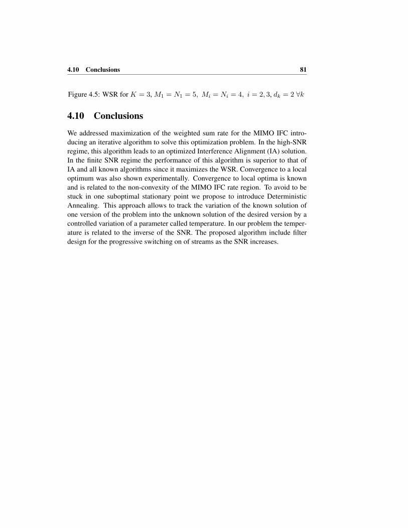
4.10 Conclusions 81
Figure 4.5: WSR for K = 3, M1 = N1 = 5, Mi = Ni = 4, i = 2, 3, dk = 2 ∀k
4.10 Conclusions
We addressed maximization of the weighted sum rate for the MIMO IFC intro-
ducing an iterative algorithm to solve this optimization problem. In the high-SNR
regime, this algorithm leads to an optimized Interference Alignment (IA) solution.
In the finite SNR regime the performance of this algorithm is superior to that of
IA and all known algorithms since it maximizes the WSR. Convergence to a local
optimum was also shown experimentally. Convergence to local optima is known
and is related to the non-convexity of the MIMO IFC rate region. To avoid to be
stuck in one suboptimal stationary point we propose to introduce Deterministic
Annealing. This approach allows to track the variation of the known solution of
one version of the problem into the unknown solution of the desired version by a
controlled variation of a parameter called temperature. In our problem the temper-
ature is related to the inverse of the SNR. The proposed algorithm include filter
design for the progressive switching on of streams as the SNR increases.

82 Chapter 4 Sum Rate Maximization for the Noisy MIMO Interference Channel

Chapter 5
Sum Rate Maximization with
Partial CSIT via the Expected
Weighted MSE
5.1 Introduction and State of the Art
In previous chapters we described two ways for beamforming design in MIMO in-
terference channel, interference alignment and maximum WSR approaches. Both
methods require perfect channel state information at both sides, transmitter and re-
ceiver. In practical systems only imperfect (estimated and often fed back) CSI is
available at each transmitter implying that more robust schemes need to be consid-
ered for beamforming design. In [131] the problem of robust beamforming design
for single user MIMO with different types of CSI has been studied. There imperfect
CSI is divided in two different classes: deterministic and stochastic (statistical). In
the deterministic case the known channel lies in an uncertainty region defined ac-
cording to some norm. In stochastic channel representation the channel knowledge
is given in term of mean and/or covariance. The design criterion described in the
paper was the minimization of the mean squared error. The authors showed that
the optimal transmit directions are the right singular vectors of the channel, channel
mean, depending if perfect or erroneous CSI are considered. The beamformer de-
sign problem for a multiuser MIMO MAC channel, in presence of statistical CSIT,
has been studied in [132]. The authors found that the optimal transmit directions,
83

84Chapter 5 Sum Rate Maximization with Partial CSIT via the Expected Weighted MSE
when the minimization of the average sum mean squared error (MSE) is studied,
were given by the eigenvectors of the channel mean or correlation matrix. [133]
considered the robust joint optimization of transmitters and receivers in a MIMO
broadcast setting where CSIT is modeled with deterministic uncertainty. In the pa-
per is proposed a framework that allows to solve different problem such as: power
minimization with MSE constraints, worst-case MSE minimization. The authors
solved this set of non convex problems introducing an iterative algorithm based on
alternating minimization optimizing transmitter and receiver in different iteration
steps reformulating the problem as a semidefinite programming.
The authors in [134] studied the problem of robust beamforming design for a MISO
interference channel under deterministic CSI uncertainty. The cost functions that
are taken into account include worst-case sum rate maximization and worst-case
minimum rate maximization. To solve the problem centralized and distributed al-
gorithms were introduced based on semidefinite programming. [135] considered
the problem of power gain region characterization in presence of perfect CSIR
and deterministic CSIT uncertainty for a MISO interference channel. To find the
optimal robust beamformers the authors cast the problem as a second order cone
program for an efficient solution. They also observe that at high SNR zero forcing
beamformers achieves full multiplexing gain if the channel uncertainty scales in-
versely proportional with the SNR, otherwise single user transmission is optimal.
In [136] the authors studied the problem of joint transceiver design for MIMO
interference channel introducing an optimization problem based on a function of
the mean squared error (MSE). They considered the sum MSE and per-user MSE
minimization providing two iterative algorithms that solve the problems using al-
ternating minimization. Apart the case when perfect CSI is available they also
solved the same problems assuming a stochastic CSI uncertainty. In [137] the au-
thors propose a robust beamforming approach for a MIMO interference channel
in presence of deterministic CSI uncertainty. Their iterative algorithm alternately
computes transmit and receive filters with the objective of maximizing the worst-
case per-stream SINR using semidefinite relaxation. [138] considered the problem
of weighted sum rate maximization of a MIMO interference channel when imper-
fect CSIT, with bounded error, is used to design transmit and receive filters. The
authors provided an iterative algorithm, based on alternating minimization, that
solved the problem reformulating it in a semi-definite programming for a more
efficient solution.

5.2 Contributions 85
5.2 Contributions
In this chapter we focus on robust beamforming design for a MIMO interfering
broadcast channel (IBC) with the objective of maximizing the sum rate when
stochastic CSIT is available while the receiver has perfect CSI. The solution pro-
posed for robust beamforming design is based on the relationship between WSR
and Weighted MSE (WMSE) [45] and chapter 4. The main difference with respect
to [131] resides in the multi user approach that makes impossible to directly use
the results derived in that paper. Here the optimal expressions of the beamforming
filters are obtained from the minimization of the sum of average WMSE, where the
expectation is taken w.r.t. channel realizations. The optimal expression obtained
for transmit and receive filters are then used to develop an iterative algorithm, based
on alternating minimization, that converges to a local optimal solution. In a recent
paper [139] a similar approach is considered. The main difference it that there
the objective is the sum MSE minimization and not the sum rate maximization as
in this chapter. Then even if the approaches look very similar the convergence
points are different. In addition we show that minimizing the expected value of
the WMSE corresponds to the maximization of a lower-bound of the WSR. Finally
we introduce some simulation results to validate numerically the proposed algo-
rithm. We compare, in term of achieved sum rate, the proposed solution with IA
beamforming design, obtained from partial and perfect CSIT, and with the solu-
tion proposed in chapter 4. We see that if the channel uncertainty scales inversely
proportionally with the SNR then there is no loss in DoF with respect to an IA
solution.
5.3 Signal Model
Figure 5.1: MIMO Interference Broadcast Channel
We consider a K-cell MIMO interfering broadcast channel (IBC), schemati-
cally reported in Fig. 5.1. For ease of exposition, we denote the transmitters as
Base station (BS) and the receivers as Mobile user (MU). The k-th BS is equipped
with Mk transmitting antennas and wants to communicate with Lk MUs in its own
cell. We denote with N(k)i the number of antennas at i-th MU in cell k. Because
all Tx-Rx pairs share the same frequency bands each transmission generates inter-
ference at all non intended receivers. At Rx number i in cell k the received signal
vector y(k)i can be written as

86Chapter 5 Sum Rate Maximization with Partial CSIT via the Expected Weighted MSE
y(k)i = H
(k)ik x(k)
i +∑
l 6=k
H(k)ik x
(k)l +
∑
j 6=k
Lj∑
l=1
H(k)ij x
(j)l + n(k)
i (5.1)
where H(k)ij ∈ CN
(k)i ×Mj represents the channel matrix between the j-th BS and i-
th MU in cell number k, x(k)i is the CMk×1 transmit signal vector of the k-th BS for
its i-th MU and the CN(k)i ×1 vector n
(k)i represents (temporally white) AWGN with
zero mean and covariance matrix Rnknk. The channel is assumed to follow a block-
fading model having a coherence time of T symbol intervals without channel vari-
ation. Each entry of the channel matrix is an independent complex random variable
drawn from a Gaussian distribution CN(0, 1). We denote by G(k)i , the CMk×d
(k)i
precoding matrix of the k-th BS to the i-th receiver. Thus x(k)i = G
(k)i s
(k)i , where
s(k)i is a d(k)
i × 1 vector representing the d(k)i independent symbol streams for the
(k, i)-th user pair. We assume s(k)i to have a spatio-temporally white Gaussian dis-
tribution with zero mean and unit variance, s(k)i ∼ N(0, I
d(k)i
). The i-th receiver, to
suppress interference and retrieve its d(k)i desired streams, applies the filter matrix
F(k)Hi ∈ Cd
(k)i ×N
(k)i .
5.4 WSR maximization for the MIMO interfering Broad-
cast channel
In this chapter we focus our attention on the maximization of the WSR of K-cell
MIMO IBC when only partial CSIT is available. In the first part of this section
we introduce the sum rate maximization problem, studied for the MIMO IFC in
chapter 4, for the K-cell MIMO IBC [44]. We limit receiver complexity by treating
the interference as colored noise, from here the definition of Noisy IBC. As a result,
linear receivers are sufficient.
Assuming Gaussian signaling, the WSR maximization problem can be mathe-matically expressed as follows:
{G⋆(k)
i
}=arg min{
G(k)
i
}
K∑
k=1
Lk∑
i=1
−u(k)
ilog |E(k)−1
i|
s. t
Lk∑
i=1
Tr(G(k)H
iG(k)
i) ≤ Pk ∀k
where E(k)i = (I + G
(k)Hi H
(k)Hik R
(k)−1
iH
(k)ik G
(k)i )−1, u(k)
i ≥ 0 denotes the weightassigned to the (k, i)-th user’s rate and Pk the corresponding transmit power con-

5.4 WSR maximization for the MIMO interfering Broadcast channel 87
straint. The interference plus noise covariance matrix R(k)
iis:
R(k)
i= Rnknk
+∑
(l,j) 6=(k,i)
H(k)
ilG(l)
jG(l)H
jH(k)H
il.
As described in chapter 4 the maximization of the WSR can be tackled introducing
an augmented cost function in which two additional optimization variables appear,
receive filters and weighting matrices W(k)i . The optimization problem that we
consider is
arg max{G(k)
i , F(k)
i , W(k)
i }
∑
(k,i)
−u(k)
i(Tr(W(k)
iE
(k)
i)− log |W(k)
i|)
(5.2)
s. t
Lk∑
i=1
Tr(G(k)Hi G(k)
i ) ≤ Pk.
Assuming E{s(k)i s(k)Hi } = I
d(k)i
, the MSE covariance matrix for general Tx and
Rx filters is
E(k)
i=E[(s(k)
i − F(k)Hi y
(k)i )(s(k)
i − F(k)Hi y
(k)Hi ]}
=I−G(k)Hi H
(k)H
ik F(k)i − F
(k)Hi H
(k)
ik G(k)i
+∑
(l,j)
F(k)H
iH(k)
ilG(l)
jG(l)H
jH(k)H
ilF(k)
i+F(k)H
iRnknk
F(k)
i
(5.3)
This cost function is concave or even quadratic in one set of variables, keeping the
other two fixed. Hence we shall optimize it using alternating maximization. Here
we consider a channel knowledge at the transmitter side that can be modeled in
term of channel mean and variance, that can represent the channel estimate and
estimation error:
H(k)
ij = H(k)
ij + (R(k)r
i )12 H
(k)
ij (Rtj)
H2 (5.4)
where H(k)
ij can model the channel estimate for the channel between Tx j and
Rx i in cell k. Rtj is the Tx side covariance matrix while R
(k)r
i represents the
covariance matrix at the Rx side. H(k)
ij is a matrix with iid Gaussian, zero mean
and unit variance, entries. We should underline here that this restrictive Kronecker
covariance model is not required for the technique described in this paper to be
applicable. We only assume this model to simplify some of the expressions.
With the given parametrization of the channel we can obtain the expected value of
the MSE:
E(k)
i=E
H|H {E(k)
i} = I−G
(k)Hi H
(k)H
ik F(k)i − F
(k)Hi H
(k)
ik G(k)i
+∑
(l,j)
F(k)H
iH(k)
ilG(l)
jG(l)H
jH(k)H
ilF(k)
i
+F(k)Hi
∑
(l,j)
Tr{RtlG
(l)
jG(l)H
j}R(k)r
i+Rnknk
F
(k)i

88Chapter 5 Sum Rate Maximization with Partial CSIT via the Expected Weighted MSE
where the expectation above is taken w.r.t. the CSI uncertainty. We should remarkthat assuming a Tx side covariance matrix of the form Rt
l = αlI then it is possible
to interpret the expected MSE above as the original MSE in (5.3) with H(k)
ij =
H(k)
ij and an augmented noise covariance matrix contribution of the form R′
nknk=
∑l αlPlR
(k)ri + Rnknk
.Hence the proposed partial CSI algorithm solves exactlythe perfect CSI WSR for a system with modified channel and noise covariancematrices! The optimization problem (5.2) now becomes the following:
arg max{G(k)
i , F(k)
i , W(k)
i
}∑
(k,i)
−u(k)
i(Tr(W(k)
iE
(k)
i)− log |W(k)
i|)
(5.5)
s. t
Lk∑
i=1
Tr(G(k)H
iG(k)
i) ≤ Pk.
The corresponding Lagrangian can be written as:
J({G(k)i ,F(k)
i ,W(k)i , λk}) = −
∑
k
λk(
Lk∑
i=1
Tr(G(k)H
iG(k)
i)− Pk)
−∑
(k,i)
u(k)
i(Tr(W(k)
iE
(k)
i)− log |W(k)
i|)
(5.6)
This new cost function will be optimized w.r.t. one set of variables, keeping theother two fixed. The first step is the calculation of the optimal Rx filters assuming
fixed the matrices G(k)i and W
(k)i . From the derivative of J w.r.t. F
(k)i the optimal
receiver results to be an MMSE filter of the form:
F(k)
i=(∑
(l,j)
[H(k)
ilG(l)
jG(l)H
jH
(k)H
il+Tr{Rt
lG(l)
jG(l)H
j}R(k)r
i]
+Rnknk)−1H
(k)
ikG(k)
i
(5.7)
The following step is the determination of the optimal expression for the matrix
W(k)i while keeping the other two variable sets fixed. Then, equating the derivative
of the Lagrangian (5.6) w.r.t. W(k)i to zero, we get :
W(k)i = E
(k)−1
i (5.8)
The final step is the maximization of the given cost function w.r.t. the BF
matrix. To accomplish this task we derive the Lagrangian w.r.t. the matrix Gk and
equate it to zero:
∂J({G(k)i
,λk})
∂G(k)∗i
= −∑
(l,j)
u(l)
jTr{W(l)
jF(l)H
jR(l)r
jF(l)
j}Rt
kG(k)
i− λkG
(k)
i
u(k)i H
(k)H
ik F(k)i W
(k)i −
∑
(l,j)
u(l)
jH(l)H
jkF(l)
jW(l)
jF(l)H
jH(l)
jkG(k)
i= 0.
5.4 WSR maximization for the MIMO interfering Broadcast channel 89
This leads to the following expression for the optimal BF:
G(k)i =
(∑
(l,j)
u(l)
j[H(l)H
jkQ(l)
jH(l)
jk+Tr{Q(l)
jR(l)r
j}Rt
k]+λkI
)−1
×H(k)H
ik F(k)i W
(k)i u(k)
i
(5.9)
where Q(l)j = F
(l)j W
(l)j F
(l)Hj . The only variable that still needs to be optimized
is the Lagrange multiplier λk. First check if the power constraint is satisfiedfor λk = 0. If yes, then λk = 0. If not, the Tx power equality constraintis active. To derive the optimal value of λk we can use the results derived inchapter 4 for the IFC. If we define the following compound quantities Fk =diag{F(k)
1 , . . . ,F(k)Lk}, Gk = [G(k)
1 , . . . ,G(k)Lk], Hij = [H(i)T
1j , . . . ,H(i)TLkj ]
T , Wk =
diag{u(k)1 W
(k)1 , . . . , u(k)
LkW
(k)Lk} and Rr
k = diag{R(k)r1 , . . . ,R(k)r
Lk} we can read the
IBC studied above as a traditional IFC. Then to find the optimal value of λk wepre-multiply the derivative of the Lagrangian J w.r.t. the compound BF matrix byGH
k . Thanks to the first order optimality condition taking the trace of that productwe get:
Tr
{GH
k
∂J({Gk, λk})∂G∗
k
}= 0.
Imposing the power constraint to be satisfied with equality, hence the contribution
λkTr {GHk Gk} = λkPk, we are able to derive the value of the optimal Lagrange
multiplier. To overcome the convergence difficulties in non-convex optimization
problems, like WSR, several heuristic approaches have been proposed. As shown
in chapter 4 we can use Deterministic Annealing (DA) since also in the WSR maxi-
mization problem the convexity properties are driven by a scalar parameters. In our
problem, the role of temperature is played by the noise power σ2k, which starting
from now we assume, without losing generality (w.l.g.), equal to σk = σ2 ∀k.
Algorithm 5 DA-MWSR Algorithm for MIMO IFC
set t = 0Fix the initial set of precoding matrices G
(k)i
repeat
increment SNR: t(i+1) = t(i) + δtrepeat
Given G(k)i compute F
(k)i and W
(k)i , ∀(k, i), as in (5.7)-(5.8)
Given F(k)i , W
(k)i , compute G
(k)i ∀(k, i), using (5.9)
until convergence
until target SNR is reached
In the algorithm description, in Algorithm 5, t(i) represents the value of the
SNR that is incremented at each step of the annealing procedure. Here we should

90Chapter 5 Sum Rate Maximization with Partial CSIT via the Expected Weighted MSE
underline that the Rx filters calculated in the proposed algorithm are not the ones
actually used at the Rx side. Those filters are based on perfect CSIR and hence
they are different compare to the one in (5.7). The MMSE Rx filter used at receiver
i in cell k will be of the form:
F(k)i = (
∑
(l,j)
[H(k)il G(l)
j G(l)Hj H
(k)Hil +Rnknk
)−1H(k)ik G(k)
i (5.10)
5.5 WSR Lower Bound with Partial CSIT
In this section we first study how the approach presented in section 5.4 is related to
the ergodic sum rate, then we introduce a new lower bound for the WSR when IA
transmit and receive filter are computed using partial CSIT. To make the presenta-
tion more clear we specify the results of the previous section to a MIMO IFC. This
does not reduce the validity of our results because the IBC can be interpreted as a
traditional MIMO IFC using the compound quantities introduced in the previous
section. To simplify the derivation of the bound we assume to work per stream in-
stead of per user. As shown in [45] working per stream does not cause a reduction
of performances.
As described in section 5.4 the rate for a K-user MIMO IFC with full CSITcan be written as:
RFCSIT =∑
(k,n)
logE−1kn
(5.11)
where Ekn indicates the MMSE of the n-th stream of user k. Then the minimumMSE for stream n of user k is Ekn = minfkn Ekn = (1 + gH
knHHkkR
−1
knHkkgkn)
−1.Vector gkn represents the n-th column of the BF matrix Gk, matrix Rkn is theinterference plus noise covariance matrix for stream (k, n). From Jensen inequalitywe have:
EHH
{∑
(k,n)
logE−1kn
} ≥ −EH
∑
(k,n)
logEH{Ekn} (5.12)
the expectation above is taken over all channel pdfs. On the other hand the ratethat we obtain once we optimize the cost function in (5.5) is
RPCSIT =∑
(k,n)
uk log(E⋆
kn)−1 (5.13)
where E⋆kn = minfkn Ekn and is equal to:
gH
knHH
kk[∑
(l,m)
[HklglmgH
lmH
H
kl+Tr{Rt
klglmg
H
lm}Rr
kl]+Rnknk
]−1Hkkgkn

5.5 WSR Lower Bound with Partial CSIT 91
where fkn is the n-th row of the Rx filter matrix Fk. From the equation above
we can see that E{Ekn} 6= E⋆kn. Calculating the expected value over the channel
uncertainty we can show that:
EH{Ekn} ≤ E
⋆
kn(5.14)
This statement can be proved easily. Assume Ekn = Ekn(fkn,Hij), and letB(fkn) = EHEkn(fkn,Hij).Now consider B(fokn) = minfkn
B(fkn) = minfknEHEkn(fkn,Hij). Then for any
Hij ,minfkn
Ekn(fkn,Hij) ≤ Ekn(fokn,Hij)
hence
EH minfkn
Ekn(fkn,Hij) ≤ EHEkn(fokn,Hij) = min
fkn
EHEkn(fkn,Hij)
From (5.14) we can conclude
EH˜H{∑
(k,n)
logE−1kn
} ≥−EH
∑
(k,n)
logE˜H{Ekn}≥−EH
∑
(k,n)
logE⋆
kn
The final relationship says that with our approach we are actually maximizing a
sum rate lower-bound.
As shown in [140] for a BC system also for a K-user MIMO IFC it is possible to
derive a SR lower bound in case of IA transmissions. The rate for the k-th UE can
be written as:
Rk = log(1 +1
σ2k
|fkHkkgk|2) (5.15)
in the following we assume that σ2k = 1. This is for the case where perfect CSIT
are available at the BSs. Here we give only the main results for the case where
each user sends only one stream dk = 1 ∀k.To study the case with imperfect CSIT, we use the channel model (5.4) where
now Hij = (Rri )
12 Hij(R
tj)
H2 . Due to IA design fk Hki gi = 0 , ∀k 6= i. Then we
rewrite the Rx signal as:
rk =fkHkkgksk + fkHkkgksk +∑
i 6=k
fkHkigisi + fknk
=fkHkkgksk + fkn′
k
where the equivalent noise term n′
k represents the residual interference plus noise
contribution that can be model as a Gaussian noise zero mean and variance σ′2k =
1 + σ2.Now absorbing all the interference contributions in the noise (we are consider-
ing the noisy IFC) we get a rate lower bound (and close approximation) by ignoring

92Chapter 5 Sum Rate Maximization with Partial CSIT via the Expected Weighted MSE
the dependence of the term fkHkkgksk on the signal sk and absorbing fkHkkgkskinto the noise also. Hence we get the rate lower bound
RLBk = log(1 +
1
σ′2k
|fkHkkgk|2) (5.16)
In other words, this rate lower bounds corresponds to the rate of an IFC with max
WSR-IA design for the case in which the overall channel is H instead to H and
the noise variances are increased by a factor σ2 in link k.
5.6 Simulation Results
We provide here some simulation results to compare the performances of the pro-
posed algorithm for the maximization of the WSR using partial CSIT (MWSRPCSI
in figure) for a 3-user MIMO IFC. Here DA is used to avoid to be trapped in local
optimal solutions. To find the IA solution for the case with partial CSIT (IAPCSI )
we use the algorithm proposed in [33] where instead of the real channel matrix
Hij we use only the channel estimate Hij . The channels are generated accord-
ing to model (5.4). The algorithm proposed in this paper can handle any general
choice of the Tx and Rx covariance matrix but in the numerical examples proposed
in this section we consider, as example, Rtj = I and Rr
i = σ2I. σ2 represents the
estimation error variance and here is scaled inversely proportional with the SNR.
In Fig. 5.2 the performances, in terms of sum rate, of the proposed robust max
WSR algorithm and IA for the case of partial CSIT are depicted. Those curves are
compared with sum rate obtained using the MWSR, from chapter 4, and IA, from
[33], with perfect CSIT (MWSRFCSI and IAFCSI respectively). It can be noted
that the max WSR solution outperforms the IA solutions for both cases, perfect and
partial CSIT. On the other hand the rate curves obtained with partial CSIT show
a rate offset compare to the corresponding curves obtained with perfect CSIT. In
Figure 5.2: Sum Rate comparisons for K = 3Mk = Nk = 2, ∀k
Fig.5.3 we report the sum rate curves for the same algorithms presented before.
The main difference is that in this case the channel estimation error variance does
not scale with the SNR but remains constant at −6dB. As we can see this implies
that the performance obtained with algorithms based on partial CSIT are charac-
terized by a saturation at high SNR. This is due to the fact that at high SNR to
keep a finite gap with the full CSIT case the channel quality should scale with the
SNR. In addition in Fig. 5.3 we report also the performance of the MWSR algo-
rithm, derived in chapter 4, when it is implemented using only the channel estimate

5.7 Conclusions 93
Hij to determine the optimal BF (MWSR w channel estimate). As we can see the
proposed algorithm (MWSRPCSI ) outperforms the former solution manifesting a
more robust behavior.
Figure 5.3: Sum Rate comparisons for K = 3Mk = Nk = 2, ∀k
5.7 Conclusions
In this chapter we studied the maximization of the WSR in the case of partial CSIT
for the Noisy MIMO IBC. The expectation of the WSR, w.r.t. the channel, is
approximated with the expectation of the WMSE. This approximate solution gives
an iterative algorithm based on alternating minimization between Tx, Rx filters and
weighting matrices. The performances of the proposed algorithm, specified for a
MIMO IFC, are compared with an IA solution calculated using the same partial
CSIT. As we were expecting maximizing the WSR outperforms the IA solution
also for the partial CSIT case. On the other hand using partial channel knowledge
causes a loss in term of SNR offset but not in term of slope. So we can conclude
that the proposed algorithm achieves, with partial CSIT, the same DoF of IA with
perfect CSIT if the CSI quality increases with the SNR.

94Chapter 5 Sum Rate Maximization with Partial CSIT via the Expected Weighted MSE

Chapter 6
CSI Acquisition in the MIMO
Interference Channel via Analog
Feedback
6.1 Introduction
With the seminal work [28] the authors have shown that interference alignment
overcomes the conventional approach of orthogonalizing the resource blocks. In
particular IA maximizes the degrees of freedom in a K user interference chan-
nel achieving, under some conditions, half the performance of a interference free
system. In [33] and in Chapter 4 has been shown that even though IA promises
maximum DoF in a MIMO IFC, it remains suboptimal at finite SNRs. To maxi-
mize the system performances, a more appropriate approach at finite SNR regimes,
is to maximize the weighted sum rate. This achieves a significant improvement, in
term of sum rate, compared to IA in medium to low SNR regimes. Both approaches
described before, WSR maximization and IA design, require that all devices have
perfect and also global channel state information (CSI). This assumption cannot
always be satisfied in practical time-varying channels. For this reason different
studies have been conducted for more practical situations.
The problem of CSI acquisition has been raised since the discovery that in sin-
gle user MIMO systems having channel knowledge at the receive side allows to
achieve very high data rates [23]. However achieving the required channel knowl-
95

96Chapter 6 CSI Acquisition in the MIMO Interference Channel via Analog Feedback
edge means that some part of the coherence time, the time period where the proper-
ties of the channel can be assumed constant, is used for the transmission of training
symbols. This causes the consequent reduction of time left for useful data transmis-
sion. In [141] the question on how much coherence time should be used for training
for a single user MIMO link is studied when only channel state information at the
receiver (CSIR) is required. In [142] the capacity of a MIMO channel with M,Ntransmitting and receiving antennas respectively is studied when accurate estima-
tion of the coefficients is generally not available to either the transmitter or the
receiver due to fast channel variations. They computed the asymptotic capacity at
high SNR in terms of the coherence time T and the number of transmit and receive
antennas, showing that the optimum DoF should satisfy d∗ = min{M,N,
⌊T2
⌋}.
[143] extended the results obtained in [141] to study the dirty paper coding
(DPC) capacity region of a MIMO BC channel. The CSI acquisition scheme is
based on downlink training and perfect channel feedback. A similar problem is
studied in [144, 145]. There the analysis is based assuming a ZF beamformer in-
stead of the more complex DPC. This approach leads to a rate lower bound that
is optimized as function of the CSI acquisition overhead. In addition also imper-
fect feedback transmission is accounted in the CSI acquisition optimization. In
[145] two feedback strategies are studied: digital or quantized and analog channel
feedback. The authors also introduced a one-step prediction channel model with
feedback delay and characterize the trade off between uplink and downlink spec-
tral efficiencies. A similar setting of [145] is studied in [140] where the authors, to
study the CSI acquisition optimization problem, introduce a new rate lower bound
of BC channel when ZF beamforming is used.
The problem of feedback in interference channel has been recently studied in
several papers [146, 147, 148]. Kramer in [146] studied a Gaussian interference
network where a noiseless and high-rate feedback link exists and informs each
transmitter of the outputs of the receiver to which it is communicating to. It is
shown that for an interference channel feedback increases capacity in the case of
strong interference. In [147] the interference channel with noisy feedback is stud-
ied. The authors introduced a new capacity outer bound that reveals that the noisy
feedback loses its usefulness when the variance of the noise on the feedback link
is larger than the noise on the forward channel. [149] focused on the two users
interference channel with generalized feedback. As generalized feedback the au-
thor described the information that is gathered at each transmitter over the wireless
media without any dedicated link where receivers feed back information to the
transmitters. A coding strategy is proposed that allows to achieve higher data rate
compared to the case without feedback. The two users Gaussian interference chan-
nel with feedback has been recently studied in [148]. The author derived achievable
schemes, based on combining different coding techniques, and new capacity outer

6.1 Introduction 97
bounds that describe the capacity region for all values of channel parameters within
2 bits per user while the symmetric capacity is determined within 1 bit.
The problem of how to use feedback for the IA design, and how the corre-
sponding rate is influenced by noisy feedback, has been treated in several recent
papers [46, 47, 150, 48]. In [46] the authors consider the SISO IFC with frequency
selective channels. Using quantized channel feedback they show that the full mul-
tiplexing gain can be achieved if the feedback bit rate scales sufficiently fast with
the SNR. This result is extended in [47] to the MISO and MIMO IFC. In both
papers the authors consider the less practical assumption that the feedback link is
represented by an error-free communication. In [150] the authors study the design
of the feedback link structure, called in the paper feedback topology, in a MIMO
IFC when IA is used as transmission strategy. Using a closed form expression for
IA beamformer, based on the result proposed in [31], the authors proposed two
types of topologies with the objective of reducing feedback overhead. The impact
of limited feedback on the system performance has also been studied. The authors
of [48] proposed to use analog feedback for the acquisition of full CSIT. The chan-
nel coefficients are directly fed back to the base stations without any quantization
process. This has the advantage, in contrast to digital feedback, that the complexity
does not increase with SNR. In [48] CSIT processing and transmitter computation
is centralized, and CSIR issues are neglected. They show that using IA with the
acquisition of CSIT using analog feedback incurs no loss of multiplexing gain if
the feedback power scales with the SNR.
A different approach has been studied in [49] where the author showed for
different selected multiuser communication scenarios that it is possible to align
the interference when the transmitters do not know the channel coefficients but
they only have information about the channel autocorrelation structure of different
users. In [49] a staggered block fading channel model is the only assumption re-
quired to achieve IA. The resulting multiplexing gain is much lower however than
for the case of full CSI. These techniques are now known by the terms delayed
CSIT or retrospective IA. A new IA approach has been introduced in [151] based on
space-time alignment that employs multi-slot transmission protocol that achieves43 DoF without any CSIT. In [50, 51] these results are extended introducing a new
transmission protocol that takes advantage of delayed CSIT and imperfect current
channel estimates. This new scheme, compare to the one in [151], exploits a com-
bination of the space-time alignment, designed for fully outdated CSIT with the
use of simple zero-forcing (ZF) precoders. Another key innovation is the retrans-
mission of the quantized version of interference generated in the previous slots in-
stead of analog retransmission. Finally in [52] the authors considered a two users
MISO IFC with time-correlated channel where each transmitter has delayed CSIT
and imperfect current CSIT, obtained from prediction. They derive the DoF re-
98Chapter 6 CSI Acquisition in the MIMO Interference Channel via Analog Feedback
gion extending the results in [50] to the MISO IFC. The problem of characterizing
the DoF region using delayed CSIT or output feedback has been the focus of re-
cent research works. The DoF region of the two-user MIMO interference channel
with delayed CSI is studied in [152]. It is shown that, depending on the antenna
dimensions, the region with delayed CSIT can be bigger than that of no CSI. In
[153] the DoF region of the two-user MIMO interference channel is studied in the
presence of noiseless channel output feedback and with delayed CSIT. The authors
proved that output feedback and delayed CSIT can enlarge the DoF region when
compared to the case in which only delayed CSIT is used. This is in contrast with
the MIMO BC channel where output feedback and delayed CSIT does not increase
the DoF region. The reason behind that is the fact the output feedback gives some
side information to each transmitter about the signal of the concurrent transmitter.
In the MIMO BC the transmitted signals come from the same transmitter then it
has full knowledge of all messages. [154] investigated the two user MIMO IFC in
fast fading channel under different feedback settings, such as Shannon feedback,
limited Shannon feedback, and output feedback, wherein all or certain form of CSI
is known at the transmitter with a finite delay. They showed that the DoF regions
with Shannon and the limited Shannon feedback, are strictly bigger than the DoF
region with just delayed CSIT under some conditions on the antennas distributions.
These results are developed introducing a new form of retrospective interference
alignment scheme that exploits transmitter cooperation made possible by output
feedback in addition to delayed CSIT. This introduces a more efficient form of
interference alignment than previously known schemes that use just delayed CSIT.
6.2 Contributions
In this chapter we introduce two transmission protocols for CSI acquisition at the
BS and MU that are based on channel training and analog feedback (FB), for both
TDD and FDD communication systems. The main difference between the two
approaches is in the FB part: channel FB or output FB. In the channel FB solution,
described also in [48] and [155], each MU feeds back to the BS the downlink
channel estimates while in the output FB scheme, the MU feeds back directly the
received samples of the DL training phase. In FDD communications uplink and
downlink transmissions can take place at the same time. Hence with output FB, it
is possible to shrink the time overhead, reducing partially the silent periods. At the
end of this chapter we consider optimizing the sum rate, by focusing in particular
on the resulting net degrees of freedom, as a function of the coherence time. This
approach allows us to easily optimize any set of parameters to unveil the trade-off
between the cost and the gains associated to CSI acquisition overhead. In particular

6.3 Transmission Phases 99
we show that if the coherence time is shorter than a certain threshold transmitting
with full DoF is no longer optimal.
6.3 Transmission Phases
We assume a block fading model, in which the channel is assumed to be con-
stant over T channel uses, called coherence time. This time period T will need
to be shared between the different training Tovrhd and data transmission phases
Tdata = T −Tovrhd of the overall transmission scheme. In this section we describe
all the necessary transmission phases required to set up a communication in the
MIMO IFC where the beamformers and receiver filters are designed to maximize
the weighted sum rate. The protocol discussed here, and also independently stud-
ied in [48], constitutes of some training (UL and DL) phases and a feedback part
where each terminal disseminates the channel state information acquired through
training. In this part we will focus our attention on a FB strategy where the chan-
nel coefficients are directly fed back as unquantized modulation symbols. This is
usually referred to as analog transmission. This protocol can be used for both TDD
and FDD communication systems but here we focus on FDD, this approach will
be justified later on in the chapter.
Figure 6.1: MIMO Uplink Interference Channel
6.3.1 Downlink Training Phase
During this phase each BSk sends orthogonal pilot sequences that can be received
by all the MU for a total duration of TDLT . In this way MUi can easily estimate
the DL channels Hi = [Hi1, . . . ,HiK ] directly connected to it. Because the com-
pound channel matrix Hi has dimensions Ni×∑
k Mk the minimum total duration
of this training phase is
TDLT ≥
K∑
k=1
Mk.
Each BS independently transmits an orthogonal matrix Ψk of dimension Mk ×TDLT with power PDL
T hence the total received Ni × TDLT matrix at Rx i is:
Yi =∑
k=1
√PDL
T HikΨk + V (6.1)
where V represents the zero mean additive white Gaussian noise with variance σ2v .
The DL Tx power can be related to the time duration of the corresponding Tx phase

100Chapter 6 CSI Acquisition in the MIMO Interference Channel via Analog Feedback
as
PDLT =
TDLT
MkP
DL
T . (6.2)
where PDL
T represents the DL power constraint. Using an MMSE estimate on YiΨl
each DL channel can be written as Hi = Hi + Hi where:
Hi ∼ N
(0,
PDLT
σ2v + PDL
T
I
), Hi ∼ N
(0,
σ2v
σ2v + PDL
T
I
)(6.3)
we call σ2
Hi
and σ2
Hi
the variance of the channel estimate and channel estimation
error respectively.
6.3.2 Uplink Training Phase
This phase can be seen as the dual of the DL training where now each MU sends
orthogonal pilots to all BSs for the estimation of the UL channel matrices. The
time duration of this phase should satisfy the following:
T ULT ≥
K∑
k=1
Nk.
Then BSk can estimate the compound channel matrix Hi = [Hi1, . . . ,HiK ] using
an MMSE estimator as described for the DL training phase. Each UL channel
can be represented in terms of channel estimate and channel estimation error with
variance respectively σ2H
and σ2
H:
Hi ∼ N
(0,
P ULT
σ2v + P UL
T
I
), Hi ∼ N
(0,
σ2v
σ2v + P UL
T
I
). (6.4)
The UL training power is now defined as:
P ULT =
T ULT
NkP
UL
T . (6.5)
where PUL
T represents the UL power constraint. We are describing all the transmis-
sion phases for the FDD transmission scheme, hence different frequency bands are
used for UL and DL communications. This separation implies that transmission
and reception can take place at the same time. If we take advantage of this possi-
bility the two training phases, UL and DL, can collapse in only one training slot
that has duration TT = max{TDLT , T UL
T }. Accounting for this new training phase
implies a reduction of the total overhead Tovrhd.
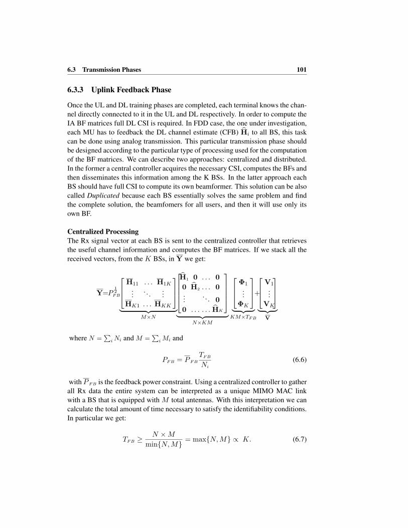
6.3 Transmission Phases 101
6.3.3 Uplink Feedback Phase
Once the UL and DL training phases are completed, each terminal knows the chan-
nel directly connected to it in the UL and DL respectively. In order to compute the
IA BF matrices full DL CSI is required. In FDD case, the one under investigation,
each MU has to feedback the DL channel estimate (CFB) Hi to all BS, this task
can be done using analog transmission. This particular transmission phase should
be designed according to the particular type of processing used for the computation
of the BF matrices. We can describe two approaches: centralized and distributed.
In the former a central controller acquires the necessary CSI, computes the BFs and
then disseminates this information among the K BSs. In the latter approach each
BS should have full CSI to compute its own beamformer. This solution can be also
called Duplicated because each BS essentially solves the same problem and find
the complete solution, the beamfomers for all users, and then it will use only its
own BF.
Centralized Processing
The Rx signal vector at each BS is sent to the centralized controller that retrieves
the useful channel information and computes the BF matrices. If we stack all the
received vectors, from the K BSs, in Y we get:
Y=P12FB
H11 . . . H1K
.... . .
...
HK1 . . . HKK
︸ ︷︷ ︸M×N
H1 0 . . . 0
0 H2 . . . 0...
. . . 0
0 . . . . . . HK
︸ ︷︷ ︸N×KM
Φ1
...
ΦK
︸ ︷︷ ︸KM×TFB
+
V1
...
VK
︸ ︷︷ ︸V
where N =∑
i Ni and M =∑
i Mi and
PFB = P FB
TFB
Ni
(6.6)
with P FB is the feedback power constraint. Using a centralized controller to gather
all Rx data the entire system can be interpreted as a unique MIMO MAC link
with a BS that is equipped with M total antennas. With this interpretation we can
calculate the total amount of time necessary to satisfy the identifiability conditions.
In particular we get:
TFB ≥ N ×M
min{N,M} = max{N,M} ∝ K. (6.7)

102Chapter 6 CSI Acquisition in the MIMO Interference Channel via Analog Feedback
To extract the i−th CFB contribution we pre-multiply the received matrix Y by
the i-th orthonormal matrix ΦHi :
YΦHi =
√PFB
Hi1...
HiK
︸ ︷︷ ︸Hi
Hi +VΦHi
then we perform a least square (LS) estimate based on the UL channel estimates
Hik: HLS
i= P
−12
FB (HH
iHi)
−1HH
i. Using this estimator we obtain the following CFB
estimates:
Hi = H
LS
i YΦHi = Hi + P
12FBH
LS
i HiHi +HLS
i VΦHi
= Hi − Hi + P12FBH
LS
i HiHi +HLS
i VΦHi = Hi − ˜
Hi
The CFB estimate can be written as a function of the true DL channel and the CFB
estimation error:Hi = Hi − ˜
Hi. The error contribution is due to the DL and UL
channel estimation errors (Hi, Hi) in the DL and UL training phases respectively.
The CFB estimation error˜Hi is distributed as N(0, σ2
˜Hi
I) where
Cov(˜Hi|Hi) = σ2
HiI+ [(σ2
Hiσ2
Hi) +
σ2
PFB
](HH
i Hi)−1.
Assuming that (HH
i Hi)−1 is distributed as an inverse Wishart matrix, then
E{(HH
i Hi)−1} ∝ 1
M−NiI. So we can write the covariance matrix as Cov(
˜Hi|Hi) =
σ2˜HiI where:
σ2˜Hi
= σ2
Hi+
1
M −Ni[(σ2
Hiσ2
Hi) +
σ2
PFB
]
Distributed Processing
In this case the CFB transmission is organized in such a way that each BS can
gather full channel knowledge from all MU. The Rx matrix at BSk can be written
as:
Yk=√PFB
[Hk1 . . .HkK
]︸ ︷︷ ︸
Mk×N
H1 0 . . . 0
0 H2 . . . 0...
. . . 0
0 . . . . . . HK
︸ ︷︷ ︸N×KM
Φ1
...
ΦK
︸ ︷︷ ︸KM×TFB
+Vk

6.3 Transmission Phases 103
where
PFB = P FB
TFB
Ni
(6.8)
with P FB is the feedback power constraint. In the distributed approach to satisfy
the identifiability conditions the CFB length should be:
TFB ≥ N ×M
mini{Mi, Ni}∝ K2 (6.9)
To extract the i−th CFB contribution we pre-multiply the received matrix Yk by
the i-th orthonormal matrix ΦHi :
YkΦHi =
√PFBHkiHi +VkΦ
Hi .
Also in this case we use a LS estimator, based on the UL channel estimate Hki,
HLS
ki= P
−12
FB (HH
kiHki)
−1HH
ki. The CFB estimate can be written as function of the
true DL channel and the CFB estimation error:Hi = Hi − ˜
Hi. The error contri-
bution is due to the DL and UL channel estimation errors (Hi, Hki) in the DL and
UL training phases respectively:
Hi = H
LS
ki YkΦHi = Hi + P
12FBH
LS
ki HkiHi +HLS
ki VkΦHi
= Hi − Hi + P12FBH
LS
ki HkiHi +HLS
ki VkΦHi = Hi − ˜
Hi
where the estimation error is then distributed as N(0, σ2˜Hi
I), with
Cov(˜Hi|Hki) = σ2
HiI+ [(σ2
Hiσ2
Hki) +
σ2
PFB
](HH
kiHki)−1
Assuming that E{(HH
kiHki)
−1} ∝ 1Mk−Ni
, we can write the covariance matrix as
Cov(˜Hi|Hki) = σ2
˜HiI where:
σ2˜Hi
= σ2
Hi+
1
Mk −Ni[(σ2
Hiσ2
Hki) +
σ2
PFB
] (6.10)
Another possible strategy to receive the analog feedback is to use linear MMSE
estimate instead of the least square approach described in this section. The two
solutions will be identical at high SNR but in different SNR regimes LMMSE
should give better performances.
The analog FB transmission described here is based on the assumption that the
number of Tx and Rx antennas satisfy the relation that min{Mi} ≥ Nj , ∀j. This
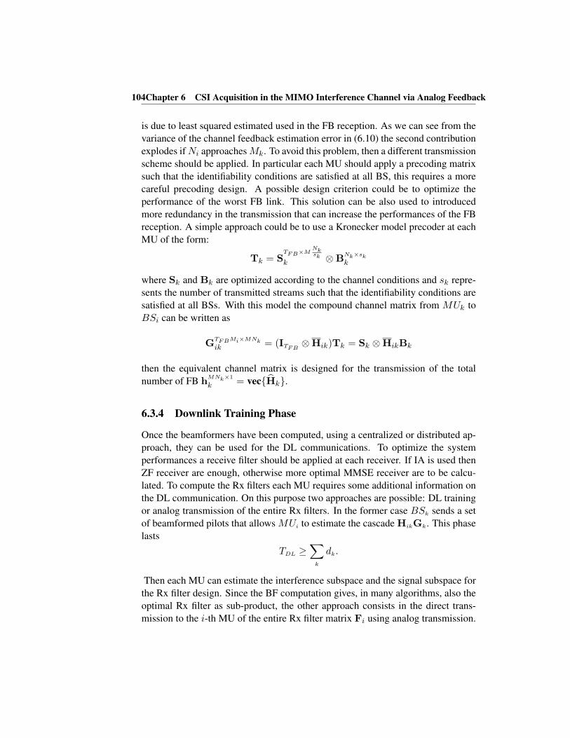
104Chapter 6 CSI Acquisition in the MIMO Interference Channel via Analog Feedback
is due to least squared estimated used in the FB reception. As we can see from the
variance of the channel feedback estimation error in (6.10) the second contribution
explodes if Ni approaches Mk. To avoid this problem, then a different transmission
scheme should be applied. In particular each MU should apply a precoding matrix
such that the identifiability conditions are satisfied at all BS, this requires a more
careful precoding design. A possible design criterion could be to optimize the
performance of the worst FB link. This solution can be also used to introduced
more redundancy in the transmission that can increase the performances of the FB
reception. A simple approach could be to use a Kronecker model precoder at each
MU of the form:
Tk = STFB×M
Nksk
k ⊗BNk×skk
where Sk and Bk are optimized according to the channel conditions and sk repre-
sents the number of transmitted streams such that the identifiability conditions are
satisfied at all BSs. With this model the compound channel matrix from MUk to
BSi can be written as
GTFBMi×MNkik = (ITFB
⊗Hik)Tk = Sk ⊗HikBk
then the equivalent channel matrix is designed for the transmission of the total
number of FB hMNk×1
k = vec{Hk}.
6.3.4 Downlink Training Phase
Once the beamformers have been computed, using a centralized or distributed ap-
proach, they can be used for the DL communications. To optimize the system
performances a receive filter should be applied at each receiver. If IA is used then
ZF receiver are enough, otherwise more optimal MMSE receiver are to be calcu-
lated. To compute the Rx filters each MU requires some additional information on
the DL communication. On this purpose two approaches are possible: DL training
or analog transmission of the entire Rx filters. In the former case BSk sends a set
of beamformed pilots that allows MUi to estimate the cascade HikGk. This phase
lasts
TDL ≥∑
k
dk.
Then each MU can estimate the interference subspace and the signal subspace for
the Rx filter design. Since the BF computation gives, in many algorithms, also the
optimal Rx filter as sub-product, the other approach consists in the direct trans-
mission to the i-th MU of the entire Rx filter matrix Fi using analog transmission.

6.3 Transmission Phases 105
This solution requires a transmission duration
TDL ≥∑
k
Nkdk
min{Nk,Mk}
The two solution proposed here are not equivalent. Which solution should be pre-
ferred depends also on the operating SNR point. For example in high SNR, where
we are interested more in maximizing the total degrees of freedom the duration of
this phase has a bigger impact compared to the estimation error, if the feed-forward
power also scales with the SNR, then DL training is the preferable solution.
In the following we consider the approach based on training. Using a sequence
of orthogonal pilots φkm for stream (k,m) of length 1×TDL, the Rx signal at MU
k is:
Ykm =√
PTHkkgkmφkm +∑
(in) 6=(km)
√PTHkiginφin +Vkm
where the two Nk × TDL matrices Ykm = [ykm[1], . . . ,ykm[TDL]] and Vkm =[vkm[1], . . . ,vkm[TDL]] represent the signal and noise contributions. The least
square estimate of the cascade channel-BF is given as:
Hklglt =1
TDL
√PT
YkmφHlt = Hklglt +
1
TDL
√PT
VkmφHlt
︸ ︷︷ ︸Hklglt
(6.11)
the elements of the estimation error matrix are distributed according to N(0, σ2
Hklglt
I),
where σ2
Hklglt
= σ2
TDLPT. Using channel estimate (6.11) we can build the MMSE
Rx filter as:
fH
km=PT
(Hkkgkm
)H
[∑
in
HkiginPT
(Hkigin
)H
+σ2I
]−1
(6.12)
We can further develop (6.11) in order to underline the dependence of the DL
channel estimate at the BSl obtained using CFB in section 6.3.3:
Hklglt =H
(l)
kl glt +˜H
(l)
kl glt + Hklglt. (6.13)
H
(l)
kl represents the DL channel estimate calculated at BSl used for the calculation
of the BF vector glt. Using the expression (6.13) and the first order approximation:
(A+∆A)−1 = A−1 −A−1∆AA−1 we can decompose the Rx filter (6.12) as:
f(l)H
km =PT
H
(l)
kkgkmR(l)−1yy
+˜f(l)H
km = f(l)H
km +˜f(l)H
km (6.14)
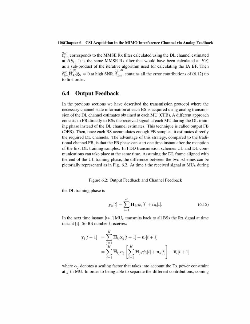
106Chapter 6 CSI Acquisition in the MIMO Interference Channel via Analog Feedback
f(l)
km corresponds to the MMSE Rx filter calculated using the DL channel estimated
at BSl. It is the same MMSE Rx filter that would have been calculated at BSl
as a sub-product of the iterative algorithm used for calculating the IA BF. Then
f(l)
kmH
(l)
kl gli = 0 at high SNR.˜f(l)H
km contains all the error contributions of (6.12) up
to first order.
6.4 Output Feedback
In the previous sections we have described the transmission protocol where the
necessary channel state information at each BS is acquired using analog transmis-
sion of the DL channel estimates obtained at each MU (CFB). A different approach
consists to FB directly to BSs the received signal at each MU during the DL train-
ing phase instead of the DL channel estimates. This technique is called output FB
(OFB). Then, once each BS accumulates enough FB samples, it estimates directly
the required DL channels. The advantage of this strategy, compared to the tradi-
tional channel FB, is that the FB phase can start one time instant after the reception
of the first DL training samples. In FDD transmission schemes UL and DL com-
munications can take place at the same time. Assuming the DL frame aligned with
the end of the UL training phase, the difference between the two schemes can be
pictorially represented as in Fig. 6.2. At time t the received signal at MUk during
Figure 6.2: Output Feedback and Channel Feedback
the DL training phase is
yk[t] =K∑
i=1
Hkiψi[t] + nk[t]. (6.15)
In the next time instant [t+1] MUk transmits back to all BSs the Rx signal at time
instant [t]. So BS number l receives:
yl[t+ 1] =
K∑
j=1
Hljxj [t+ 1] + nl[t+ 1]
=
K∑
j=1
Hljαj
[K∑
i=1
Hjiψi[t] + nk[t]
]+ nl[t+ 1]
where αj denotes a scaling factor that takes into account the Tx power constraint
at j-th MU. In order to being able to separate the different contributions, coming

6.5 TDD Vs FDD transmission strategy 107
from different MUs, we assume to use time multiplexing. Each BS has to estimate
all the matrices Hi = [Hi1, . . . ,HiK ]Ni×M . To estimate this many coefficients
the required total length of the output FB phase is:
T oFB ≥ N ×M
mini{Ni,Mi}(6.16)
Comparing equation (6.16) with (8.6) we can see that there is no reduction in the
length of the FB phase using OFB comparing to traditional channel FB. The reduc-
tion of the overhead comes from partial elimination of silent periods, as shown in
Fig.6.2. The DL overhead time due to CSI acquisition for the case of OFB can be
quantified as:
TDLovrhd = (T o
FB + 1) + TDL
while for CFB we have:
TDLovrhd = TDL
T + T oFB + TDL.
From the equations above we see that using OFB we save TDLT − 1 time instants.
We should also study the case where the UL and DL coherence periods are
aligned, Fig. 6.3. In this situation the gain obtained using OFB instead of CFB is
reduced. The total time overhead in the DL transmission becomes:
TDLovrhd = TUL
T + T oFB + TDL.
The gain of using the OFB solution is now given as: ∆T = TDLT −TUL
T = N−M .
Figure 6.3: Output Feedback and Channel Feedback with aligned coherence peri-
ods
6.5 TDD Vs FDD transmission strategy
Usually TDD transmission is used arguing that thanks to reciprocity the amount
of feedback required to acquire CSIT is (significantly) reduced. In this communi-
cation strategy MUi does not need to feedback channel Hki to BSk because this
information can be acquired using the corresponding UL channel Hki. On the other
hand this information is needed at the other base stations BSj 6=k for the design of
their own BF matrix. From this observation we realized that for distributed BF
process the organization of feedback is very complicated if we consider the possi-
bility of reducing feedback using reciprocity, and hence we can conclude that TDD

108Chapter 6 CSI Acquisition in the MIMO Interference Channel via Analog Feedback
does not help in reducing the feedback overhead compared to FDD transmission
scheme. On the contrary if we consider a centralized BF calculation then TDD
makes feedback not required because the reduced set of CSI available at each BS
using reciprocity is shared and hence the computation center can collect the total
required information on the DL channels based on the UL channel estimates avail-
able at each BS. For the reasons above we developed all the transmission phases
only for FDD transmission.
6.6 From Practical to more Optimal Solutions
All the different transmission phases described in section 6.3 are done one after
the other but other solutions are possible to optimize the overhead. In a possible
alternative approach, one does not need to wait to gather all CSIT before start-
ing transmission. For example one user can start to transmit directly after the DL
training phase as a single user MIMO link without any CSIT. Or it also is possi-
ble to start with blind/noncoherent IA first. Then, instead of going from K = 1to full K immediately another possible strategy is to build intermediate IA solu-
tions. We gradually increase the number of interfering links as soon as the corre-
sponding transmitters acquire the required CSI to design the IA beamformers for
the given interfering subsystem. Another consideration is that when the (analog)
channel feedback duration is non-minimal, beamformers can be computed imme-
diately after the minimum number of feedback coefficients has been obtained and
DL transmission can start. Then the beamformers can get further updated during
the remaining feedback transmission using better channel estimates. This is one
advantage of analog feedback (similar to repetition coding), that ”decoding” can
be done before the full ”codeword” has been received. In any case, there is a myr-
iad of possibilities for alternative solutions, to increase the system performances
using a more optimized transmission strategy.
6.7 DoF optimization as function of Coherence Time
In [48] the authors show that using analog feedback of channel estimates it is pos-
sible to achieve the same DoF as IA if the feedback power is scaled as the SNR.
Here our goal is different, we want to optimize the number of transmitted streams
as a function of coherence time. The rationale behind this optimization problem is
the following. If the coherence time is not long enough to host the total overhead
due to CSI acquisition then the transmission of dtot =∑
k dk is no longer possi-
ble regardless of the amount of power used for the feedback transmission phase.
Then we should use blind IA or noncoherent transmission techniques. Another
6.7 DoF optimization as function of Coherence Time 109
possibility is to reduce the total amount of transmitted streams. The reduction of dimplies a reduction of the required number of active transmit and receive antennas
as well as the number of transmitting users, so that the amount of CSI exchange
is optimized as a function of the coherence time. In this section our objective is
the optimization of system parameters, number of antennas and number of users,
that allow us to maximize the net DoF, defined as the number of DoF that are actu-
ally achievable taking into account the overhead due to CSI acquisition. Our cost
function then becomes:
maxn,m,k
J(n,m, k) = maxn,m,k
(1− Tovrhd(n,m, k)
T
)kd(n,m, k) logSNR (6.17)
where m ∈ [1, N ], n ∈ [1, N ], k ∈ [1,K] (to simplify we assumed an IFC of
the form (N,N, d)K) represent the number of active transmit and receive antennas
respectively and number of active users. Tovrhd = TDLT +TFB +TDL takes into
account the DL training phase, necessary for CSIT acquisition, UL feedback phase
and beamformed training, sometimes also called dedicated training. To solve this
problem we should be able to define a relationship between the number of trans-
mitted streams and antennas. If we assume IA transmission we can relate antennas,
users and achievable streams using the following [37]:
d ≤ m+ n
k + 1. (6.18)
Since our objective is the maximization of the total DoF in the network we assume
that each user applies a transmit/receive technique that maximizes the achievable
DoF, so transmit and receive filters are designed according to IA. This transmission
strategy has the objective to maximize the achievable DoF reducing at maximum
the interference subspace dimensions generated at each non intended receiver. The
solution does not depend on the direct channel matrix but only on the interfer-
ence matrix that each transmitter generates. This allows us to reduce partially the
number of channel coefficients that need to be fed back by each MU to all BS. In
particular each MU needs to feedback only the (k−1) interfering channel matrices
for a total of (k− 1)mn coefficients. In addition only the subspace spanned by the
interference channel matrix is of relevance for the design of IA beamformers (that
is defined up to a square n × n matrix). We can conclude that the total number of
channel coefficients, that need to be fed back for IA beamforming, is :
Nc = kn[(k − 1)m− n]+. (6.19)
this will have an influence on the feedback phase duration TFB . According to
recent results on IA feasibility [38] we know that relation (6.18) is exact only for

110Chapter 6 CSI Acquisition in the MIMO Interference Channel via Analog Feedback
square symmetric IFC of the form (m,m, d)k where each user is equipped with the
same number of antennas m and transmits the same number of streams d. For this
reason we focus on this kind of system to develop our analysis. Equation (6.18)
becomes:
d ≤ 2m
k + 1. (6.20)
Before studying a MIMO IFC it is also of interest to start the analysis with simpler
and more intuitive cases: SIMO/MISO IFC. To study the MISO and SIMO case
we assume a centralize processing of the feedback.
In a SIMO IFC only the MU is equipped with multi-antenna array then only
CSIR is necessary to establish a communication. This simplifies the expression
of the time overhead that becomes: Tovrhd = k, since only one pilot per user is
enough to estimate the DL channels at each MU. In addition each BS can send only
one useful data stream, then the total number of DoF is dtot = min{k,m}. The
optimization function (6.17) then becomes (in the rest of the section we neglect the
dependence on the SNR since it is not an optimization variable):
J(m, k) = [T − k] min{k,m}
Two cases are then possible: m ≤ k or m ≥ k.
m ≤ k
The cost function becomes:
J(m, k) = [T − k]m
this function is not convex (the Hessian is indefinite) then to find the optimum in
the optimization domain we optimize the cost function over different borders of
[1, N ]× [1,K]
• Border m∗ = 1
Since the cost function J(m, k) is linear in k with coefficient −1 then the
optimum is in the left extremum of the domain, in this case k∗ = m∗ = 1.
• Border m∗ = N
Similarly to the case above k∗ = min{N,K}.
• Border k∗ = 1
Since the cost function J(m, k) is linear in m with coefficient (T − k∗) > 0then the optimum lies on the right extremum of the domain, in this case
m∗ = k∗ = 1.
• Border k∗ = K
Similarly to the case above m∗ = min{N,K}.

6.7 DoF optimization as function of Coherence Time 111
m ≥ k
The cost function can be written as:
J(m, k) = [T − k]k
that is independent of m then we can choose it minimum possible value: m∗ = k∗.
Now optimizing w.r.t. k we get
m∗ = k∗ = min{N,K,T
2}. (6.21)
From this result we can see that the optimum number of active antennas and users is
equal and varies as T2 . This is an intuitive result because in SIMO IFC the number
of DoF is equal to min{k,m} then having an excess of antennas, compared to
number of users, does not give any advantage in terms of DoF. Similarly, in the
case of more user than antennas, there are users that cannot be served without
interference, so an excess of users is only decremental in term of DoF.
The MISO IFC is characterized by a cost function that is different from the
one of the SIMO case. In this system to set up a transmission CSIT is required at
each BS, then also feedback from MUs is necessary. The time overhead, due to
CSI acquisition is then composed of DL training and feedback, we can neglect the
dedicated training phase. The cost function becomes:
J(m, k) = [T − (2k − 1)m+ 1]min{m, k}
This cost function should be treated similarly to the SIMO case since it has an
indefinite Hessian. Also in this case having the same number of Tx antennas and
active users is the optimal solution. Equating the derivative of the cost function,
assuming m = k, w.r.t. m we obtain the optimal solution of the form:
m∗ = k∗ = min{N,K,1
6(1 +
√6T + 7)}. (6.22)
Also in this case the result is intuitive since similar considerations to the SIMO
case can be stated about the number active users and Tx antennas. The different
solution obtained in the MISO case is due to the different overhead necessary to
set up a communication compared to the SIMO case, that is simpler so require less
time to achieve the required CSIR to establish a communication.
Now we study the case of a MIMO IFC of the form (m,m, d)k, that as we
said before is the case where the relationship (6.18) between users, antennas and
DoF is exact. We can study two possible cases, first we study the setting in which
the feedback processing is done in a centralized way and then we focus on the
distributed solution, proposed in section 6.3.3.

112Chapter 6 CSI Acquisition in the MIMO Interference Channel via Analog Feedback
Centralized Square MIMO
In the centralized case the total length of the time overhead is:
Tovrhd=TDLT +TFB+TDL= 2
k2 + k − 1
k + 1m
where TFB = NcKmin{m,n} . We can write (6.17) as follows for the case under
investigation:
J(m, k) =
(T − 2
k2 + k − 1
k + 1m
)2k
k + 1m (6.23)
this function is non convex hence we need to find the optimum over the borders of
the optimization domain. In order to have a feeling on how the problem behaves
as function of the coherence time what we propose is to study the cost function in
the point (N,K). We want to understand when the full MIMO IFC is no longer
optimal and hence some dimensions are shrunk if the coherence time T is shorten
than a certain threshold. In particular we study the derivative of the cost function
J(m, k) w.r.t m and k separately evaluated at the point (N,K) and we find that:
∂J(m, k)
∂m= T − 4
k2 + k − 1
k + 1m
∣∣∣∣m=Nk=K
= T − 4K2 +K − 1
K + 1N (6.24)
∂J(m,k)∂k = 2m
(k+1)2T − 4k3+3k2+3k−1
(k+1)3m2
∣∣∣∣m=Nk=K
= 2N(K+1)2
T − 4K3+3K2+3K−1(K+1)3
N2
(6.25)
now we study the sign of those derivatives as function of the coherence time T . In
particular we study when, for example,∂J(m,k)
∂k
∣∣∣∣m=Nk=K
≤ 0. This means that the
cost function evaluated at the point (N,K) is decreasing with k then if we use a
k1 < K we have that J(N,K) < J(N, k1) so to maximize J(m, k) we need to
reduce the number of active users. Similar reasoning is valid for m. Solving this
problem we find that
∂J(m,k)∂m ≤ 0 if T ≤ Tm = 4N K2+K−1
K+1
∂J(m,k)∂k ≤ 0 if T ≤ Tk = 2N K3+3K2+3K−1
(K+1)
(6.26)
It is easy to verify that Tk > Tm ∀K,N , then the first quantity that decreases
if the coherence time decreases is the number of users k. If we evaluate Tm, Tk
for any arbitrary m, k we find that Tk > Tm, ∀k,m. In addition the sign of

6.7 DoF optimization as function of Coherence Time 113
the derivative of J(m, k) w.r.t. m calculated in (N, k = 1) is always positive for
T > 2N , when it starts to becomes negative. We can conclude that the antennas
and users distribution as function of coherence time behaves as follows:
1. T > Tk
Full (N,K) MIMO IFC is optimal, then dtot =2KNK+1
2. Tk ≤ T ≤ 6N
The number of user is not full, then (N, k∗) MIMO IFC is optimal where
k∗ : k3+3k2+(3− T2N )k− (1+ T
2N ) = 0, the total DoF are dtot =2k∗(T )Nk∗(T )+1
3. 6N ≤ T ≤ 2N
SU-MIMO with N antennas is optimal so dtot = N
4. T ≤ 2N
Now also the number of antennas starts to shrink as m∗ = min{N, T2 } that
determines dtot = m∗
What is remarkable in this analysis is the simple intuition that if the coherence
time is too short SU-MIMO transmission is the best approach is indeed optimal. In
addition, if we fix the number of transmit and receive antennas to be the same, as
the coherence time start to reduce, it is optimal to reduce the number of users first
up to the point SU-MIMO. The DoF behavior as function of the coherence time
is schematically sketched in Fig. 6.4. If the coherence time is long enough then
full DoF is achieved in the MIMO IFC, then reducing the coherence time implies
that the number of user is reduced. This determines also a reduction of achievable
DoF dtot =2k∗(T )Nk∗(T )+1 until SU-MIMO is achieved. Finally if we further decrease T
then also the number of active antennas starts to decrease, then the achieved DoF
is given by the SU-MIMO formula as dtot = min{N, T2 }
Figure 6.4: Behavior of the optimized DoF distribution for square symmetric
MIMO IFC
Distributed Square MIMO
In the distributed case the total length of the time overhead is:
Tovrhd=TDLT +TFB+TDL=
k2 + 1
k + 1km
where TFB = Ncmin{m,n} . The cost function that we need to optimize becomes:
J(m, k) =
(T − k2 + 1
k + 1km
)2k
k + 1m (6.27)
114Chapter 6 CSI Acquisition in the MIMO Interference Channel via Analog Feedback
As for the centralized case this cost function is non convex. To study the behavior
of the antennas and users distribution as function of the coherence time we proceed
using the same approach of the centralized case. From the partial derivatives of the
cost function J(m, k) w.r.t. to m and k separately, evaluated in the point (N,K),we get:
∂J(m, k)
∂m=
2k
k + 1T − 4
k2 + 1
(k + 1)2k2m
∣∣∣∣m=Nk=K
=2K
K + 1T − 4
K2 + 1
(K + 1)2K2N
(6.28)
∂J(m,k)∂k = 2m
(k+1)2T − 4k3+4k2+1
(k+1)3km2
∣∣∣∣m=Nk=K
= 2N(K+1)2
T − 4K3+4K2+1(K+1)3
KN2.
(6.29)
Now studying the sign of those derivative we obtain:
∂J(m,k)∂m ≤ 0 if T ≤ Tm = 2NKK2+1
K+1
∂J(m,k)∂k ≤ 0 if T ≤ Tk = 2NKK3+2K2+1
K+1
(6.30)
As for the centralized case Tk > Tm ∀K,N , then the first quantity that decreases
if the coherence time decreases is the number of users k. We can finally summarize
the behavior of m and k as follows:
1. T > Tk
Full (N,K) MIMO IFC is optimal, then dtot =2KNK+1
2. Tk ≤ T ≤ 4N
The number of user is not full, then (N, k∗) MIMO IFC is optimal where
k∗ : k4 + 2k3 + (1− T2N )k − T
2N = 0, the total DoF are dtot =2k∗(T )Nk∗(T )+1
3. 4N ≤ T ≤ 2N
SU-MIMO with N antennas is optimal so dtot = N
4. T ≤ 2N
Now also the number of antenna starts to shrink as m∗ = min{N, T2 } that
determines dtot = m∗
Up to this point we have focused on a MIMO IFC constraining the system to have a
symmetric square MIMO structure. If we want to relax this constraint the optimiza-
tion problem becomes even more complex since the number of receiving antenna

6.7 DoF optimization as function of Coherence Time 115
now becomes an optimization variable. In this situation the relation between users,
antennas ans streams becomes:
d ≤ m+ n
K + 1.
As explained before this equation is not always exact for non square systems then
for some points in the optimization domain the cost function, constructed using
this relation, is not exact. The cost function (6.17) then becomes, for example in
the centralized case:
J(n,m, k) = (T − Tovrhd)k
k + 1(m+ n) (6.31)
where
Tovrhd = km+kn[(k − 1)m− n]+
kmin{m,n} +k
k + 1(m+ n) (6.32)
From the definition of the time overhead above we can see that for a fixed k three
different regimes can be observed in m and n.
n > (k− 1)mIn this case no alignment can be done so the entire processing should be done at
the receiver. This can be seen from the following reasoning. Consider the k = 2MIMO IFC. According to [25] the total number of DoF in the network are dtot =min{n, 2m}. If n streams are sent then with n antennas per user all the streams
can be received with simple ZF receivers. On the other hand if 2m streams are
transmitted this means that 2m < n so also in this case simple ZF receiver can
be used to retrieve the transmitted streams. Consider now a general k > 2 user
IFC. In the case where n > (k − 1)m the space spanned by the columns of the
interference channel matrix at user i, HIi = [Hi,1, . . . ,Hi,i−1,Hi,i+1, . . . ,Hi,k],does not have any overlap so no alignment can be done at the transmitter [39].
Then all the processing should be done at the Rx side. This means that only CSIR
necessary. Since each user has n antennas a maximum of d = n/k streams per
user can be sent, this implies that the minimum number of Tx antennas per user
is m = nk . To acquire the necessary CSIR a total DL training period of length
TDL = kd = n is necessary so the optimization function (6.31) becomes:
J(n) = (T − n)n
from the equation above we can see that the optimum number of Rx, and conse-
quently Tx, antennas, is {n∗ = min{N, T2 }
m∗ = n∗
k

116Chapter 6 CSI Acquisition in the MIMO Interference Channel via Analog Feedback
n ≤ m
The time overhead becomes:
Tovrhd = km+ (k − 1)m− n+ kk+1(m+ n) =
2k2+2k−1k+1 m− n
k+1
(6.33)
then cost function (6.31) becomes:
J(n,m, k) =
(T − 2k2 + 2k − 1
k + 1m+
n
k + 1
)k
k + 1(m+ n)
m ≤ n < (k− 1)mIn this case Tovrhd becomes:
Tovrhd = km+ [(k−1)m−n]nm + k
k+1(m+ n) =k(k+2)k+1 m+ k2+k−1
k+1 n− n2
m
(6.34)
then the cost function is:
J(n,m, k) =
(T − k(k + 2)
k + 1m− k2 + k − 1
k + 1n+
n2
m
)k
k + 1(m+ n)
Solving the problem outlined above is not easy, what could be done is to develop a
similar analysis proposed for the square symmetric MIMO case, where we studied
the sign of the different partial derivatives. For example in the case m ≤ n <(k − 1)m we find that the coherence times where the three derivatives, calculated
at the point (N,N,K) become negative, are:
Tk ≤ 2N K3+3K2+3K−1K+1
Tm ≤ 4N K(K+2)K+1
Tn ≤ 4N K2−2K+1
(6.35)
From the values found above we have that Tk > Tm > Tn, ∀K > 1. This im-
plies that if the coherence time decreases below Tk then the derivative of J(n,m, k)w.r.t. k, evaluated in (N,N,K) becomes negative and hence full MIMO IFC, of
the form (N,N,K), is no longer optimal and hence we should reduce the number
of active users.

6.8 Conclusions 117
6.8 Conclusions
Optimal joint transmit and receive filter design, in MIMO IFC, assumes that each
device has full channel knowledge of the entire network. This condition can not
be always satisfied in real time-varying channels. To overcome this difficulty we
analyzed a transmission protocol for the necessary CSI acquisitions at each BS and
MU. The entire process is based on training and analog FB transmission. We also
introduce the approach of output feedback where each MU feeds back directly the
received samples during the DL training phase. In FDD communications this tech-
nique allows us to shrink the time overhead reducing partially the silent periods.
Finally we optimized the sum rate of the MIMO IFC under investigation by focus-
ing in particular on the resulting degrees of freedom. We showed that the optimal
number of streams should vary as function of the channel coherence time. In addi-
tion if the coherence time is too short we showed that in some condition SU-MIMO
transmission is optimal.

Part II
Cognitive Radio Channel
Chapter 7
Beamforming for the Underlay
Cognitive MISO Interference
Channel
7.1 Introduction and state of the art
Cognitive Radio (CR) is a set of techniques permitting an efficient utilization of
the spectrum. This new communication paradigm allows spectrum reuse between
legacy (primary) networks (PN) and secondary (possibly opportunistic) networks
(SN) as long as the latter do not hamper the formers’ communications in an overly
adverse fashion. Different transmission paradigms have been introduced to de-
scribe the communication in a cognitive environment according to the level of co-
operation between primary and secondary users [58]. In this chapter we focus
on the underlay deployment. According to its definition an underlay CR commu-
nication is said to be in place when a given concerted level of interference from
secondary Tx,usually called Interference temperature constraint [55], may be tol-
erated at the primary user (PU), refer to [58] for more on CR terminology.
Underlay CR using multiple antennas has recently come under intense focus
since in such systems spatial dimensions can be exploited to shape interference
towards primary users. One of the first attempt to study how it is possible to ex-
ploit the spatial dimension at the secondary users in a cognitive radio setting is
reported in [64]. In this work the trade off between maximizing the secondary
119

120Chapter 7 Beamforming for the Underlay Cognitive MISO Interference Channel
user’s rate and controlling the interference caused at the primary receivers is stud-
ied for different CR settings. The authors exploit multi-antenna at the secondary
transmitter to design the optimal transmit filter that effectively balances between
spatial multiplexing for the secondary transmission and interference avoidance at
the primary receivers. In [156] the cognitive beamformer design problem is stud-
ied with the objective of maximizing the secondary link throughput and satisfy a
set of SINR constraints, at the secondary users, as well as limiting the interference
caused to the primary users. In the proposed algorithm a user selection schedul-
ing is also introduced. [157] addressed the problem of beamformer design to limit
the probability of interference leakage at the primary receivers. The approach in
[158] finds the beamformer weights, in presence of CSI errors, such that a set of
SINR target are met limiting the interference power at the primary receivers to be
below a fixed threshold. The problem of downlink beamforming and power alloca-
tion techniques at the cognitive base station that also ensure efficient control of the
interference caused at primary receivers while maintaining a minimum required
SINR for the secondary users is studied in [65, 159, 67]. There the secondary net-
work is always represented as a BC channel that wants to communicate in presence
of a set of primary receivers.
Much of the work in underlay CR systems has been done in the context of sec-
ondary broadcast (BC) networks coexisting with primary users. This is essentially
due to relatively good understanding of BC beamforming and power allocation
problem acquired in recent years [75] [76] based on the principle of UL-DL duality.
Using this duality, the BF designed in the virtual (dual) uplink mode can be used in
the actual downlink problem to achieve the same SINR values by choosing appro-
priate downlink power allocations. The design of secondary Tx beamformers under
primary interference constraints has, for example, been studied in [160, 161, 162]
with the objective of SINR balancing in the SN. In [160, 161] the role of UL-DL
duality principle remains instrumental in the solution of this problem. In [159, 67]
the BF at secondary base station is found introducing a new duality principle that
allows to develop a simple iterative algorithm for the power minimization problem
where a set of SINR constraints at the secondary Rxs and maximum interference
powers level at the primary receiver are imposed. In [67] a robust version of the
solution proposed in [159] is introduced. [162] addressed the problem of robust
beamforming design with uncertainties in the channel, bounded by an Euclidean
ball, the problem is modeled as a semidefinite program and is solved using a new
technique without relaxing the rank constraints. In [163] the goal was to design
optimal beamformers and rate allocation for the secondary users in a distributed
fashion in order to maximize the smallest weighted rate among secondary users.
This optimization problem includes a weighted sum-power constraint on the sec-
ondary users as well as the interference margin constraints imposed by the primary

7.2 Contributions 121
receivers. In [164] the authors studied the problem of joint transmit-receive filter
design in MIMO cognitive broadcast channel with the objective of minimizing the
total transmit power while targeting a fixed set of quality of service (QoS) require-
ments at the secondary multi-antenna receivers. At the same time the interference
caused at each primary receiver, also equipped with multiple antennas, should be
kept under a fixed threshold. When perfect CSIT is available, at the cognitive BS,
they propose an iterative algorithm that solves the problem exactly. When the re-
duced cooperation with the primary users is such that perfect knowledge of the
primary link is not available a robust algorithm is introduced to limit the interfer-
ence to the primary with high probability. Both solutions rely on the conversion of
the original problem into a Second Order Cone Programming (SOCP). In [68] the
objective was to optimize the secondary network sum rate under the interference
constraints at PUs. In this chapter the secondary network is model as an MISO
interference channel that tries to optimize its own rate in presence of a primary
receiver, the solution proposed is based on an iterative dual subgradient algorithm.
7.2 Contributions
In this chapter we focus on a secondary network (SN) that is no longer a BC but
a MISO IFC. There is one fundamental difference between linear BF design and
power allocation problems in BC and IFC, namely there are individual power con-
straints in the latter as opposed to a total power constraint in the former. Never-
theless, we argue that minimizing total Tx power in the IFC still makes sense from
green wireless point of view and thus still makes a valid optimization problem.
Here we focus on beamformer design of a secondary network, which is repre-
sented by a MISO interference channel (IFC), in presence of primary interference
constraints. The main result in this work is that we use recent results on duality
for IFC [12] and CR [159], to solve the optimization problem. With this analysis
the primary users can be seen as set of receivers in the DL communication while
as virtual primary Tx in the UL phase, thus as supplementary interference link that
the secondary BSs should take into account while designing the Rx filter in the
UL communication. We propose an iterative algorithm that efficiently solves the
power minimization problem, at the secondary network, while a set of interference
constraints are imposed on primary receivers.
7.3 MISO Cognitive Interference Channel
Fig. 7.1 depicts the cognitive radio scenario that we study in this work. The sec-
ondary system is represented as a K-user MISO IFC with K transmitter-receiver
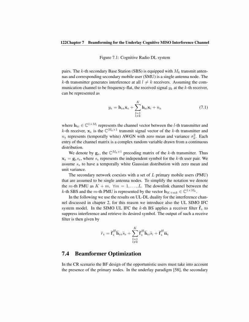
122Chapter 7 Beamforming for the Underlay Cognitive MISO Interference Channel
Figure 7.1: Cognitive Radio DL system
pairs. The k-th secondary Base Station (SBS) is equipped with Mk transmit anten-
nas and corresponding secondary mobile user (SMU) is a single antenna node. The
k-th transmitter generates interference at all l 6= k receivers. Assuming the com-
munication channel to be frequency-flat, the received signal yk at the k-th receiver,
can be represented as
yk = hkkxk +K∑
l=1l 6=k
hklxl + nk (7.1)
where hkl ∈ C1×Ml represents the channel vector between the l-th transmitter and
k-th receiver, xk is the CMk×1 transmit signal vector of the k-th transmitter and
nk represents (temporally white) AWGN with zero mean and variance σ2k. Each
entry of the channel matrix is a complex random variable drawn from a continuous
distribution.
We denote by gk, the CMk×1 precoding matrix of the k-th transmitter. Thus
xk = gksk, where sk represents the independent symbol for the k-th user pair. We
assume sk to have a temporally white Gaussian distribution with zero mean and
unit variance.
The secondary network coexists with a set of L primary mobile users (PMU)
that are assumed to be single antenna nodes. To simplify the notation we denote
the m-th PMU as K + m, ∀m = 1, . . . , L. The downlink channel between the
k-th SBS and the m-th PMU is represented by the vector hK+mk ∈ C1×Mk .
In the following we use the results on UL-DL duality for the interference chan-
nel discussed in chapter 2, for this reason we introduce also the UL SIMO IFC
system model. In the SIMO UL IFC the k-th BS applies a receiver filter f k to
suppress interference and retrieve its desired symbol. The output of such a receive
filter is then given by
rk = fHk hkksk +
K∑
l=1l 6=k
fHk hklsl + f
Hk nk
7.4 Beamformer Optimization
In the CR scenario the BF design of the opportunistic users must take into account
the presence of the primary nodes. In the underlay paradigm [58], the secondary
7.4 Beamformer Optimization 123
users are allowed to transmit if the interference caused to the primary users is
below a fixed threshold. The interference caused at the primary receiver can be
handled in different ways. In this work we assume that the secondary BS are
equipped with multiple antennas and hence can use the spatial dimension to satisfy
the interference constraints.
7.4.1 CR Beamformer Design Under Per User Power Constraint
In the CR setting that we study the SBSs want to optimize their transmit BFs such
that the total transmitted power is minimized while a set of quality of service (QoS)
constraints, here expressed in term of target SINRs, are imposed at each SMU. At
the same time the secondary network should be designed in such a way that the
total interference power at each primary receiver is below a certain fixed threshold.
From a mathematical point of view the optimization problem that we need to solve
can be represented as follow:
min{gk}
K∑
k=1
gHk gk
gHk gk ≤ Pk; k = 1, . . . ,K
s.t. SINRDLk =
gHk hH
kkhkkgk∑l 6=k gH
l hHklhklgl+σ2
k
≥γk; k = 1, . . . ,K
IDLm =
∑Kk=1 g
Hk hH
K+mkhK+mkgk ≤ 1γK+m
; m = 1, . . . , L.
(7.2)
The last inequality, in the optimization problem, represents the interference power
constraint at each primary receiver and γK+m is a measure related to the interfer-
ence level IDLm at mth PU.
The additional interference constraint in the cognitive optimization problem
can now be related to virtual SISO primary Tx/Rx pairs in the cognitive IFC. This
nevertheless does not change the structure of the problem if one considers further
fictitious primary transmitting powers [159], pm, m = K + 1, . . . ,K + L to the
corresponding PU while causing zero interference to the K links (receivers) of
the secondary network. Introducing this modification the interference constraint in
(7.2) can be rewritten as:
1
IDLm
=pK+m∑K
k=1 gHk hH
K+mkhK+mkgk
≥ γK+m; m = 1, . . . , L (7.3)
with this equivalent expression the primary interference constraint can be inter-
preted as a fictitious additional SINR constraint at the primary receiver, where
γK+m is the target SINR at PMUK+m. The optimization problem for the BF de-
sign can be solved with standard optimization tools like Lagrange multipliers, then

124Chapter 7 Beamforming for the Underlay Cognitive MISO Interference Channel
the Lagrangian of the optimization problem reported above is:
L(λi, µi,gi)=K∑
k=1
gHk gk +
K∑
i=1
µi
[gHi gi − Pi
]
+K∑
i=1
λi
− 1
γigHi hH
ii hiigi +∑
l 6=i
gHl hH
il hilgl + σ2i
+L∑
m=1
λK+m
[−pK+m
γK+m+
K∑
k=1
gHk hH
K+mkhK+mkgk + σ2K+m
](7.4)
where λk represents the Lagrange multiplier of the k-th SINR constraint and
µk is the Lagrange multiplier associated to the Tx power constraint at user k.
From the Lagrangian reported above we can write the Lagrange dual problem
of the original optimization problem (7.2) as:
max{λk},{µk},{pK+m},
K∑
k=1
λkσ2k −
L∑
m=1
λK+mpK+m
γK+m−
K∑
k=1
µkPk
s.t. − λkγkhHkkhkk +
K+L∑
l 6=k
λlhHlkhlk + ηkI�0; k = 1, . . . ,K
λk ≥ 0; k = 1, . . . ,K + Lµk ≥ 0; k = 1, . . . ,K
(7.5)
where ηk = µk + 1.The Lagrange dual of the DL beamforming problem (7.2) can be rewritten as anequivalent UL optimization problem for the Rx filter:
fk = (
K+L∑
l 6=k
λlhHlkhlk + ηkI)
−1hHkk (7.6)
then (7.5) can be rewritten [90]:
max{λk},{µk},{pK+m},
K∑
k=1
λkσ2k −
L∑
m=1
λK+mpK+m
γK+m
−K∑
k=1
µkPk
s.t. SINRULk =
λkfH
k hHkkhkkfk
fH
k
K+L∑
l 6=k
λlhHlkhlk + ηkI
fk
≤γk; k = 1, . . . ,K
λk ≥ 0; k = 1, . . . ,K + Lµk ≥ 0; k = 1, . . . ,K
(7.7)
7.4 Beamformer Optimization 125
Figure 7.2: Cognitive Radio UL system
in the equivalent UL optimization problem the Lagrange multipliers λl can be
interpreted as dual UL Tx powers and µk represents a dual noise variance. Both
quantities should now be optimized.
The original optimization problem (7.2) is expressed in the form of quadrati-
cally constrained quadratically programming that is in general non convex prob-
lems but it is possible to show that it can be expressed as a second order cone
program that, at the contrary, is a convex problem [91].
The cost function and the constraints are quadratic in the optimization variables gk,
then introducing a phase shift such that hkgk ∈ R does not influence the optimal
solution. Then the optimization problem can be rewritten as:
min{gk}
K∑
k=1
gHk gk
gHk gk ≤ Pk; k = 1, . . . ,K
s.t. (1 + 1γk)|hkkgk|2≥
∑kl=1 |hklgl|2 + σ2
k; k = 1, . . . ,K
∑Kk=1 |hK+mkgk|2 ≤ 1
γK+m; m = 1, . . . , L.
(7.8)
Introducing the following quantities:
Hk =
hk1 0 . . . 0...
. . .
0 . . . 0 hkK
; HK+m =
hK+m1 0 . . . 0...
. . .
0 . . . 0 hK+mK
both of dimensions K×∑
k Mk, gT = [gT1 , . . . ,g
TK ]T we can further rewrite (7.8)
as:
min{gk}
K∑
k=1
gHk gk
√Pk ≥ ‖gk‖2; k = 1, . . . ,K
s.t.√(1 + 1
γk)hkkgk≥
∥∥∥∥[Hkg
σk
]∥∥∥∥2
; k = 1, . . . ,K
√1
γK+m≥ ‖HK+mg‖2; m = 1, . . . , L.
(7.9)
where ‖.‖2 denotes the Euclidean vector norm. The problem above is a quadratic
problem with second order cone programming constraints that is a convex problem.
126Chapter 7 Beamforming for the Underlay Cognitive MISO Interference Channel
We can also state that the duality gap between the original problem (7.2) and the
dual problem (7.5) is zero because the optimization problem in convex hence strong
duality holds. This implies that the optimal solution of the dual problem is also
optimal for the original one.
From the modified expression of the UL optimization problem (7.7) we can see
that introducing the per user power constraint brings to introduce a fictitious noise
variance in the dual problem that should also be determined. At the optimum the
SINR constraints in the UL and the DL problems must be satisfied with equality
[159, 164], using this relationship it is possible to derive the DL BF from the UL
receiver filter. Because a scaling factor in the receiver filter at the BS does not
affect the SINR it is possible to show that the optimal DL BFs are given by:
gk =√pk fk (7.10)
where pk is such that the SINRs in the DL are satisfied with equality so:
p = (D−1 −Φ)−1σ (7.11)
where matrices D and Φ are defined as:
[Φ]ij =
{fHj hH
ijhijf j , j 6= i
0, j = i(7.12)
D = diag{ γ1
fH1 hH
11h11f 1
, . . . ,γK
fHKhH
KKhKKfK
}. (7.13)
In a similar way we can find the UL transmit powers such that the SINR constraints
in the UL are satisfied with equality:
SINRULk =
λkfHk hH
kkhkkfk
fHk
K+L∑
l 6=k
λlhHlkhlk + ηkI
fk
=γk; k = 1, . . . ,K
The slack variable pK+m has been introduced in the optimization procedure such
that the primary user interference constraints are always satisfied with equality,
then we have:
pK+m = (
K∑
k=1
gHk hH
K+mkhK+mkgk)γK+m
using pK+m the corresponding Lagrange multiplier λK+m can also be found. The
last variable that needs to be optimized is the Lagrange multiplier associated to the

7.4 Beamformer Optimization 127
per-user power constraint µk. To find the optimal value what we propose to use a
subgradient method [165] of the form:
µ(i)k = µ
(i−1)k + t(i)(g
(i)Hk g
(i)k − Pk)
where t(i) represent the step size at iteration i. The proposed algorithm is summa-
rized in Algorithm 6.
Algorithm 6 Beamformer Design in CR Setting
Initialize: i = 0, λ(0)k = 1, ∀k = 1, . . . ,K + L, µ
(0)k = 1, ∀k = 1, . . . ,K
repeat
i = i+ 1For k = 1, . . . ,K find the UL receiver filter as
f(i)
k =(
K+L∑
l 6=k
λ(i−1)l hH
lkhlk + η(i−1)
k I)−1hHkk
Update λ(i)k as
λ(i)k =
f(i)H
k (∑K+L
l 6=k λ(i−1)l hH
lkhlk + η(i−1)
k I)f(i)
k
1γkf(i)H
k hHkkhkkf
(i)
k
Determine the optimal DL BF g(i)k using (7.11)
For m = 1, . . . , L update the quantity
p(i)K+m = (
K∑
k=1
g(i)Hk hH
K+mkhK+mkg(i)k )γK+m
and find the UL power λ(i)K+m = λ
(i−1)K+mp
(i)K+m
Update µ(i) using the subgradient method with step size t(i)
µ(i)k = µ
(i−1)k + t(i−1)(gH
k gk − Pk) (7.14)
until convergence
In the iterative algorithm the Lagrange multiplier λK+m, associated to the in-
terference power constraints, are calculated as λ(i)K+m = λ
(i−1)K+mp
(i)K+m. The rational
behind this formula is the following: if the interference generated at PMUK+m
is below the threshold 1γK+m
, then p(i)K+m is less then one, this means that λ
(i)K+m

128Chapter 7 Beamforming for the Underlay Cognitive MISO Interference Channel
at the next iteration, should be reduced. If this is the case it contributes less in the
calculation of the BF vectors in (7.6), then the BF will try to spend less effort to
suppress the interference that it causes to PMUK+m. On the other hand, when
the interference is above the threshold, p(i)K+m is greater than one, then λ
(i)K+m is
increased, compare to the previous iteration. In this case the BFs at the secondary
network will spend more effort to suppress interference to that particular PMU.
7.5 Simulation results
In this section we report the numerical performance of the proposed iterative algo-
rithm for the optimization of the BF filter at the CR network in presence of a set
of primary interference constraints. The performance of Algorithm 6 is compared
with the one of a second algorithm that solves the Lagrange dual problem (7.5) us-
ing the interior-point-method where the linear matrix inequality (LMI) constraints,
that represents the dual UL SINR is handled using a logarithmic barrier [92]. Since
strong duality holds solving the dual problem provides also the optimal solution for
the the original problem (7.2). In Fig. 7.3 is plotted the Normalized Root Mean
Square Error (NRMSE) of the proposed algorithm,
NRMSE =
√1N
∑Nn=1
∑Kk=1(‖g
(i)k (n)‖2 − ‖g∗
k(n)‖2)2√1N
∑Nn=1
∑Kk=1(‖g∗
k(n)‖2)2
where ‖g(i)k (n)‖2 represents the Euclidean norm of the DL BF determined using
the iterative algorithm at iteration (i) for the n-th Monte Carlo run and g∗k(n) is the
DL BF obtained using the interior point method. The CR scenario that is simulated
is represented by a secondary IFC of K = 5 users with M = 9 Tx antennas each
and L = 5 PU. The target SINR are γk = 6 for all SUs and the interference
constraints are γK+m = 1, ∀m, and the noise variance is equal to −10dB. As we
Figure 7.3: NRMSE for K = 5, L = 5,M = 9
can see the algorithm manifests good convergence behavior.
7.6 Conclusions
In this chapter we studied the problem of beamforming design in MISO cognitive
IFC with objective the minimization of the total transmitted power. Our optimiza-
tion problem included also a set QoS constraints at each secondary receiver, in ad-
dition the total interference generated at each primary receiver should not exceed

7.6 Conclusions 129
a fixed threshold. We solved the problem using new results on UL/DL duality for
CR channel. The primary users can be seen as a set virtual primary Txs in the UL
communication, thus supplementary interference links that should be considered
in the secondary Rx design in the UL communication. We proposed an iterative
algorithm that efficiently solves the BF design problem.

130Chapter 7 Beamforming for the Underlay Cognitive MISO Interference Channel
Chapter 8
Spatial Interweave TDD
Cognitive Radio Systems
8.1 Introduction and state of the art
In the previous chapter we focused on the Underlay CR paradigm while here we
study a more stringent cognitive radio setting called Interweave (IW). In this sit-
uation a CR system exploits the unused communication resources, called white
spaces, of the primary system in an opportunistic fashion. In this communication
paradigm, secondary transmission can take place only if it does not cause any in-
terference to the primary users. We can read the interweave paradigm as a more
constrained underlay problem where the level of interference is zero. The un-
used primary resources can be time, frequency or, as recently introduced, space.
Since we focus on a secondary system that relies on the spatial dimensions to op-
portunistically setup a communication, without deteriorating the primary system’s
transmission, we refer to this setting as Spatial Interweave cognitive radio.
In [166] a MISO CR setting is considered where the cognitive transmitter de-
signs its BF in order to maximize the secondary received power with the constraint
of causing zero interference to the primary receivers.
A MIMO broadcast (BC) cognitive radio scenario is studied in [167], they
propose a Grassmannian beamforming technique for a limited feedback-based CR
network based on the null space of the primary user channels. Cooperation between
primary and secondary system is assumed.
131

132 Chapter 8 Spatial Interweave TDD Cognitive Radio Systems
In [70] the authors considered an heterogeneous system where the primary and
secondary communications can coexist only if the latter keeps under control the in-
terference generated at the primary receiver. They propose an iterative algorithm to
design the secondary system transmission parameters to maximize the secondary
users rate while imposing a maximum interference constraint to the primary re-
ceiver or the more stringent constraint of zero interference to the primary system.
The proposed algorithm is completely decentralized and is based on iterative water
filling (IWF). The author provide also an analytical description of the performances
using the game theory framework. In this work the authors do not investigate how
the cognitive users can acquire all the necessary information on channels and pri-
mary communication. In [73] a more practical setting is studied. They consider a
system model where a primary and a secondary pair of users want to coexist and
the secondary communication should take place without causing any interference
to the primary receivers exploiting the spatial dimensions. Interestingly in this
work any a-priory knowledge is assumed at the secondary network but the nec-
essary information is acquired during a learning phase that exploit reciprocity of
the primary TDD communication strategy. During this phase also partial knowl-
edge of the primary signal subspace is acquired. They underline that the proposed
scheme is better, in terms of degrees of freedom (DoF), than the previously pro-
posed scheme in [64] because partial knowledge of the Rx subspace at the primary
receivers increases the number of streams that can be Tx from the CTx. The authors
call this opportunistic way of transmission of the secondary system as opportunis-
tic spatial sharing.
The authors of [72] studied the same setting of [73] but with the objective of
making their work more practical. A transmission scheme of three phases is intro-
duced where the primary-to-secondary channel is acquired, then the channel be-
tween secondary users is estimated and finally the transmission takes place. In the
proposed analysis the secondary channel estimation errors are taken into account in
the secondary BF design and the interference caused at the secondary receiver, due
to primary communication, is reduced introducing a receive filter at the secondary
receiver.
In [168] the Pareto boundary of a secondary users’ rate region is characterized.
There the opportunistic system is described as a MISO interference channel with
a set of additional constraints of causing no interference to the primary receivers.
In addition a greedy secondary user selection algorithm is introduced to maximize
the achievable sum rate.
In the spatial interweave scenario the secondary transmitter can use Interfer-
ence Alignment [28] to design its transmitted signal. The primary receiver sees the
opportunistic transmission as interference but only in dimensions that it does not
use for its communication. As a result there is no degradation of the performance

8.2 Contributions 133
of the primary system. This beamforming technique has been proposed in [169]
where it is called opportunistic interference alignment. The authors assume perfect
knowledge of all channels without investigating how to obtain this information. As
shown in [170] acquisition of channel state information (CSI) is of crucial impor-
tance in a non cooperative system as the one considered here. The present work
includes an inventory of tools needed to render coexistence of the two systems
possible. In particular, the difficult problem of CSI acquisition is addressed. It is
shown that the solution relies on Time-Division Duplex (TDD) mode of operation.
TDD is desirable since, in theory, it allows the exploitation of uplink → downlink
reciprocity of the underlying radio propagation channel. Using this transmission
strategy the transceiver can obtain DL (UL) channel knowledge using an estimate
of the UL (DL) channel. In this work, we prove that TDD is not just a possible
option, but that it is crucial for spatial IW CR to work if unrealistic overheads
and communications between the two systems are to be avoided. Unfortunately
in practice, even in TDD, the channel reciprocity assumption only holds for one
component of the overall channel, namely the propagation channel itself. More
precisely, in order to exploit channel reciprocity one needs to compensate for the
mismatch between the analog Tx/Rx circuitry at both ends: this process is called
calibration. The calibration problem is generally addressed through two different
approaches denoted as absolute and relative calibration [171]. The first one uses
a third-party equipment, used as reference, in order to estimate and compensate
the analog Tx/Rx circuitry impairments [172] offline. In the latter approach, UL
and DL channel estimates obtained at each side of the communication link are ex-
changed at a low-rate from which calibration factors are deduced. New algorithm
for relative channel calibration has been proposed in [173].
8.2 Contributions
In this chapter we study the joint optimization of the transmit-receive filter in a
spatial interweave cognitive radio channel. The setting studied in this work is not
novel, we describe the entire communication protocol required to acquire the nec-
essary information at primary and secondary users in a spatial interweave cognitive
radio setting. What really differentiates our work with previously proposed solu-
tions, for example [73] and [72], is that no-one has studied, up to now, how to really
get channel reciprocity in real TDD transmission using UL DL channel calibration.
In addition we also underline how calibration influences transmit and receiver filter
design at primary and secondary devices. In this paper we use relative calibration
method to compensate for Tx/Rx electronics [171].
An important result that comes out of our analysis is that even though the op-
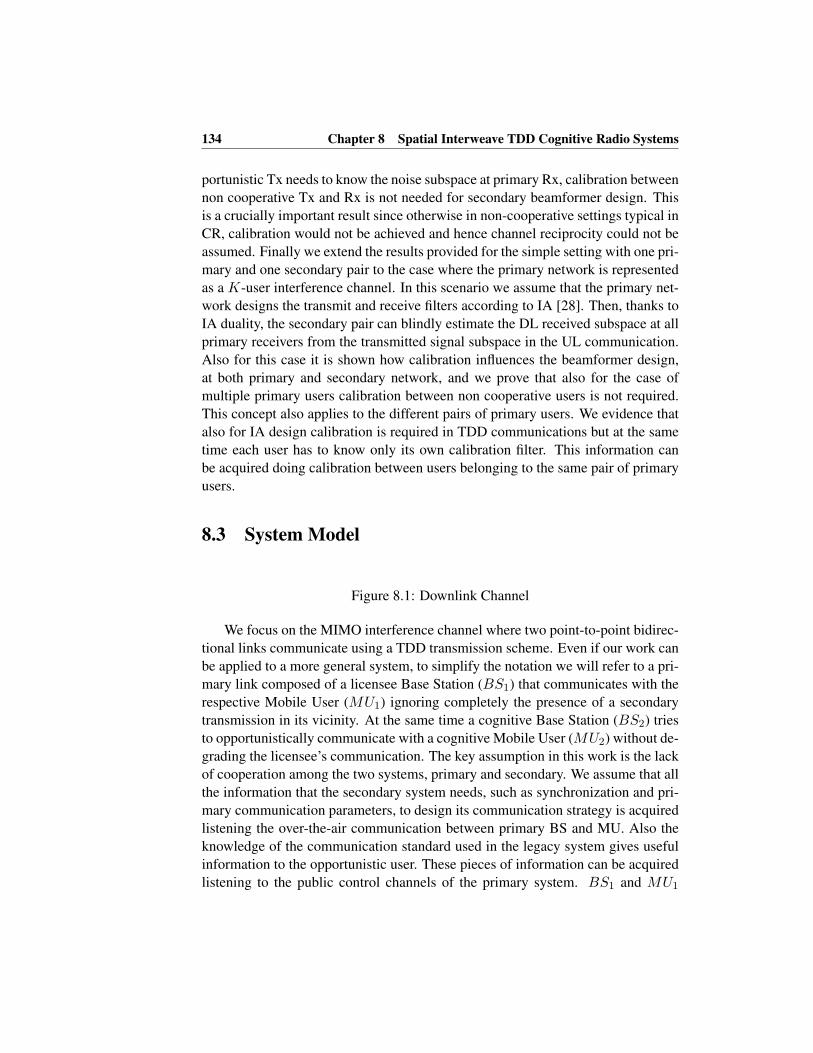
134 Chapter 8 Spatial Interweave TDD Cognitive Radio Systems
portunistic Tx needs to know the noise subspace at primary Rx, calibration between
non cooperative Tx and Rx is not needed for secondary beamformer design. This
is a crucially important result since otherwise in non-cooperative settings typical in
CR, calibration would not be achieved and hence channel reciprocity could not be
assumed. Finally we extend the results provided for the simple setting with one pri-
mary and one secondary pair to the case where the primary network is represented
as a K-user interference channel. In this scenario we assume that the primary net-
work designs the transmit and receive filters according to IA [28]. Then, thanks to
IA duality, the secondary pair can blindly estimate the DL received subspace at all
primary receivers from the transmitted signal subspace in the UL communication.
Also for this case it is shown how calibration influences the beamformer design,
at both primary and secondary network, and we prove that also for the case of
multiple primary users calibration between non cooperative users is not required.
This concept also applies to the different pairs of primary users. We evidence that
also for IA design calibration is required in TDD communications but at the same
time each user has to know only its own calibration filter. This information can
be acquired doing calibration between users belonging to the same pair of primary
users.
8.3 System Model
Figure 8.1: Downlink Channel
We focus on the MIMO interference channel where two point-to-point bidirec-
tional links communicate using a TDD transmission scheme. Even if our work can
be applied to a more general system, to simplify the notation we will refer to a pri-
mary link composed of a licensee Base Station (BS1) that communicates with the
respective Mobile User (MU1) ignoring completely the presence of a secondary
transmission in its vicinity. At the same time a cognitive Base Station (BS2) tries
to opportunistically communicate with a cognitive Mobile User (MU2) without de-
grading the licensee’s communication. The key assumption in this work is the lack
of cooperation among the two systems, primary and secondary. We assume that all
the information that the secondary system needs, such as synchronization and pri-
mary communication parameters, to design its communication strategy is acquired
listening the over-the-air communication between primary BS and MU. Also the
knowledge of the communication standard used in the legacy system gives useful
information to the opportunistic user. These pieces of information can be acquired
listening to the public control channels of the primary system. BS1 and MU1

8.4 Transmission Techniques and Channel Estimation 135
are both equipped with N1 antennas, BS2 and MU2 have both N2 antennas. The
results that we present in this paper can be easily generalized for the case of ter-
minals with an arbitrary number of Tx and Rx antennas, Mi, Nj , i, j = {1, 2}respectively. We focus on the case where the opportunistic users have a number of
antennas greater than or equal to the primary users N2 ≥ N1. We denote with (.)the quantities in the UL transmission, then matrices Hij and Hij ∈ CNi×Nj are, re-
spectively, the DL and UL channel matrices from transmitter j to receiver i, where
i, j ∈ {1, 2}. The entries of these matrices are i.i.d. complex Gaussian random
variables N(0, 1). We assume that all channels follow a block-fading model hav-
ing a coherence time of T symbol intervals without variations. This corresponds to
assuming that the channel remains constant for a sufficient number of TDD slots.
In a TDD transmission scheme, assuming perfect Tx/Rx calibration, the UL
channel is the transpose of the relative downlink one [171] due to channel reci-
procity.
Hij = HHji (8.1)
Thus an UL channel estimate can be used for designing the transmit beamformer
in the DL communication. We assume that channel estimates are obtained through
pilot symbols.
8.4 Transmission Techniques and Channel Estimation
In the Interweave cognitive scenario, licensee (primary) systems are not aware of
the presence of secondary systems which should ideally cause no interference. The
primary Tx is therefore assumed to be a Single User MIMO link (SU-MIMO). In
this system the transmitter and receiver filters are designed in order to maximize
the transmission rate. The capacity-achieving solution is based on a Beamform-
ing matrix obtained from the singular value decomposition (SVD) of the channel
matrix combined with Water-Filling power allocation [174]. Assuming low-rank
Tx, the primary link can be decomposed into a signal and a complementary (noise)
subspace,
H = U∆VH = [UsUn]
[∆s
∆n
] [VH
s
VHn
](8.2)
where subscripts s or n refer to signal subspace and noise subspace respectively.
The matrices U and V are unitary matrices and ∆ is a diagonal matrix that contains
the singular values of the channel matrix. In order to waterfill in UL and DL, both
BS1 and MU1 must have complete knowledge of the primary channel and Rx noise
variances. This information can be obtained partially through TDD reciprocity
(pilots for channel estimation) and partially through (unavoidable) feedback.

136 Chapter 8 Spatial Interweave TDD Cognitive Radio Systems
In the interweave scenario unlicensed users must transmit without disturbing
the licensed transmission. Because at low to medium signal-to-noise ratios (SNR)
the primary transmitters are expected to exploit a limited number of channel modes,
the opportunistic transmitter can beamform its signal in the noise subspace of the
licensed communication. This has been labeled as interference alignment tech-
nique in [169]. To adapt its communication, the secondary Tx has to know the
signal subspace of the primary Rx. As discussed in the following this subspace can
be learnt by an opportunistic exploitation of the primary system signals.
All TDD frames in both UL and DL are composed of two time segments, one
comprising possibly multiple data streams and the second pilots for channel esti-
mation. In the primary link only the data part of the frame is beamformed but not
the pilots. This implies that they span the entire channel space. On the other hand
in the cognitive link, pilots are also beamformed, thus ensuring that they do not
interfere with the primary transmission. We assume that the secondary TDD slots
are aligned with the primary slots using classical spectrum sensing and synchro-
nization techniques.
8.4.1 First TDD Slot
In this first slot all devices in the system should start to acquire the channel state
information they need. In particular the licensed BS transmits without knowledge
of the downlink channel and therefore cannot beamform. MU1 can estimate the
channel matrix H11 using pilots. The DL channel matrix has dimension N1 ×N1,
then the minimum training length should satisfy :
TPT ≥ N1 (8.3)
The primary BS sends orthogonal pilots with power P PT that can be represented
as a matrix ΨP of dimension N1 × TPT . The total received N1 × T P
T matrix at the
primary MU is:
Y1 =√
P PT H11ΨP + V (8.4)
where V represents the zero mean additive white Gaussian noise with variance σ2v .
The DL Tx power can be related to the time duration of the corresponding Tx phase
as
P PT =
T PT
N1P
P
T . (8.5)
where PP
T represents the DL power constraint. Using an MMSE estimate on Y1Ψ1
each DL channel can be written as H11 = H11 + H11 where:
H11 ∼ N
(0,
P PT
σ2v + P P
T
I
), H11 ∼ N
(0,
σ2v
σ2v + P P
T
I
)(8.6)

8.4 Transmission Techniques and Channel Estimation 137
we call σ2H11
and σ2
H11
the variance of the channel estimate and error respectively.
During this phase, cognitive users in particular MU2, can use the pilot symbols
of the primary communication to opportunistically estimate the cross channel H21.
A similar analysis of (8.6) can be done for the channel H21 = H21 + H21.
8.4.2 Second TDD Slot
Figure 8.2: Uplink Channel
MU1 now knows the downlink channel matrix and hence it can construct the
beamforming subspace TMU1 ∈ CN1×d1 using reciprocity in equation (8.1). In
the same UL frame BS1 can estimate the UL channel, as done for the DL channel
in the previous slot, exploring pilot symbols incorporated in each time segment.
d1 represents the number of transmitted streams, obtained using WF, and is equal
to the signal subspace dimension. The received signal at BS1 has the following
structure.
y1 = H11TMU1s1 + n1 (8.7)
y1 ∈ CN1×1 is the received signal vector, s1 ∈ Cd1×1 is the transmitted signal
vector and n1 ∈ CN1×1 is the spatially white Gaussian noise with zero mean and
variance σ21 .
MU1 proceeds with a SVD decomposition of the downlink dual channel, H11 =HH
11 = V1∆11UH1 , uses as Tx beamformer TMU1 = U1,s, taking the columns
of U1 according to the WF solution. The BS1 can design its Rx filter as RBS1 =VH
1,s ∈ Cd1×N1 from the SVD of the UL channel. The signal at the output of the
receiver filter at BS1 is written as
r1 = RBS1H11TMU1s1 +RBS1n1
= VH1,sH
H11U1,ss1 +VH
1,sn1 = ∆11,ss1 + n′
1(8.8)
where ∆11,s is the diagonal matrix containing singular values of HH11 correspond-
ing to the signal subspace. Vector n′
1 is the post-processed noise vector that, thanks
to the unitary propriety of the Rx filter, preserves the distribution of the original
noise vector and hence has variance σ21 .
At BS2 the N2 × 1 Rx signal is given by
y2 = HH12TMU1s1 + n2 = HH
12U1,ss1 + n2. (8.9)
Assuming sufficient data samples at BS2, we can obtain a consistent estimate of
the primary Tx signal subspace from the autocorrelation matrix of the Rx signal
138 Chapter 8 Spatial Interweave TDD Cognitive Radio Systems
Ry2y2= E{y2y
T2 }. In practice we use the sample covariance matrix for the
process of blind subspace estimation
Ry2y2=
1
TE
TE∑
t=1
y2[t]yH2 [t]. (8.10)
From the eigenvalue decomposition of (8.10), Ry2y2= UΛUH , we can estimate
the signal space dimension d1 using the information theoretic criteria described
in [175]. Then we can determine the primary noise subspace estimate Un from
the last N2 − d1 eigenvector of U. This approach gives a consistent estimate for
sufficient data samples TE while for finite data samples the estimate is affected by
an estimation error [176] that can be characterized as
Un = Un − Un = SH†
2 NHUn (8.11)
where N = [n2[1], . . . ,n2[TE]] and
S2 = HH12TMU1 [s1[1], . . . , s1[TE]]︸ ︷︷ ︸
S2
. (8.12)
A† denotes the pseudo-inverse of A. In a similar way it is possible to determine
the estimation error of the primary signal subspace Us [177]. Due to channel
reciprocity the Tx and Rx signal subspace in the primary link are the same, hence
the knowledge of the primary Tx subspace is sufficient to determine the Rx signal
subspace at MU1.
Knowing Us, the BS2 Tx beamformer TBS2 ∈ CN2×d2 can send at most d2streams while ensuring its signal lies in the noise subspace at the primary Rx. This
implies that
RMU1H12TBS2 = 0 =⇒ TBS2 ⊆ (RMU1H12)⊥. (8.13)
The equation above says that TBS2 belongs to the subspace spanned by
span(RMU1H12)⊥, where (RMU1H12)
⊥ represents the orthogonal complement
of the row space of the matrix RMU1H12. In our case a possible choice for the
secondary transmit filter is TBS2 = Un.
Including the receiver at MU1 in the definition of TBS2 has the advantage
that in the low to medium SNR of the primary link, where the primary Tx sends
only d1 < N1 of the total available signaling dimension N1, the secondary Tx can
(opportunistically) transmit at most d2 ≤ N2 − d1 streams. On the other hand in
the high SNR region, when the primary link uses up its entire degrees of freedom
(DoF) for spatial multiplexing, the secondary can always transmit d2 ≤ N2 − N1
streams.

8.4 Transmission Techniques and Channel Estimation 139
8.4.3 Third TDD Slot
From this TDD time slot onwards starts the steady state of the system. This means
that also the cognitive BS starts to transmit to MU2. As for the reverse link, in the
primary forward link BS1 constructs its beamforming subspace using SVD of the
channel matrix H11. Then the transmit beamformer is TBS1 = V1,s, and MU1
uses as receiver RMU1 = UH1,s. In this slot also the opportunistic BS starts to
transmit its data symbols, hence the received signal at primary MU is
y1 = H11TBS1s1 +H12TBS2s2 + n1. (8.14)
In order to extract the useful data MU1 applies the Rx filter to the received signal:
r1 = RMU1y1. BS2 beamformed signal lies in the noise subspace (8.13), hence
MU1 sees no interference. On the other hand MU2 receives signals from both
BS1 and BS2:
y2 = H22TBS2s2 +H21TBS1s1 + n2. (8.15)
MU2 needs to estimate the noise and signal subspaces of the primary commu-
nication to design its beamformer. This can be done using semi-blind estimation
procedure. The definition semi-blind comes from the fact that part of the infor-
mation is obtained using usual training and the remaining information comes from
blind subspace estimation.
Using the beamformed pilots incorporated into the secondary data frame, the sec-
ondary receiver can estimate the cascade of secondary direct channel and beam-
former H22TBS2 that has dimensions N2 × d2. The training length should now
satisfy:
T ST ≥ d2. (8.16)
Once the secondary direct link has been estimated, MU2 has to estimate the sig-
nal and noise subspaces of the primary DL transmission. To accomplish this task
the cognitive device can reconstruct the transmitted signal from BS2 during the
secondary pilot transmission and then subtract it from the Rx signal vector:
y′
2 = y2 − H22TBS2s2 = H21TBS1s1 + n2. (8.17)
In (8.17) we assume the estimate H22TBS2 is obtained without error to simplify
the analysis.
Using the reconstructed signal y′
2 MU2 determines the signal and noise sub-
spaces, denoted as Vs and Vn respectively, of the primary downlink signal using
second-order statistics (SOS). This estimation procedure can follow the same steps
as the one proposed in section 8.4.2. The estimated noise and signal subspace will
be also affected by similar error contribution of (8.11).

140 Chapter 8 Spatial Interweave TDD Cognitive Radio Systems
Finally MU2 designs its beamformer subspace such that it creates zero interference
at the primary BS:
TMU2 ⊆ (RBS1HH21)
⊥ (8.18)
a possible choice is TMU2 = Vn.
8.4.4 Fourth TDD slot
In this slot all nodes have the required knowledge to transmit to corresponding
receivers. The received signal of the primary UL transmission is
y1 = HH11TMU1s1 +HH
21TMU2s2 + n1 (8.19)
The Rx filter at BS1 suppresses the opportunistic signal, transmitted from MU2,
thanks to the proper design of TMU2in (8.18). The received signal at BS2 never-
theless contains interference due to MU1.
y2 = HH22TMU2s2 +HH
12TMU1s1 + n2. (8.20)
To suppress this interference contribution standard linear MIMO receiver can be
used.
8.5 Secondary Link Optimization
The secondary link beamformer subspace, designed to cause zero interference at
the primary receivers, is invariant to a multiplication by a square d2 × d2 matrix
QBS2 ,TBS2QBS2 ∈ span(TBS2) hence RMU1H12TBS2QBS2 = 0 . The remain-
ing degrees of freedom in QBS2 can be used for the optimization of the secondary
link communication.The received signal at MU2 is given in (8.15). To find the matrix QBS2 we
need to solve the following optimization problem:
maxQBS2
log
∣∣∣∣∣∣∣I+QH
BS2TH
BS2HH
2,2R−1intH2,2TBS2︸ ︷︷ ︸K
QBS2
∣∣∣∣∣∣∣s.t. Tr(TBS2QBS2Q
HBS2
THBS2
) ≤ P2
(8.21)
where P2 represents the transmit power constraint at the secondary link and Rint =H2,1TBS1S1T
HBS1
HH2,1+σ2
nI is the interference plus noise covariance matrix with
S1 = E{s1sH1 }. We use the common notation |A| = det(A). The Lagrangian ofthe optimization problem in (8.21) can be written as:
L = log∣∣I+QH
BS2KQBS2
∣∣− λ[Tr(TBS2QBS2QHBS2
THBS2
)− P2]. (8.22)
8.5 Secondary Link Optimization 141
where λ represents the Lagrangian multiplier associated to the secondary user
power constraint P2. Introducing the eigenvalue decomposition K = UK∆KUHK
,
the matrix QBS2 can be parametrized as QBS2 = UKP1/2
2 , where P1/2
2 represents
a diagonal matrix with the power allocation for the d2 streams. Then (8.22) can be
rewritten as:
L = log |I+∆KP2| − λ(Tr(UHKTH
BS2TBS2UK︸ ︷︷ ︸
D
P2)− P2)
=
d2∑
i=1
log(1 + δipi)− λ(
d2∑
i=1
Diipi − P2)
(8.23)
To determine the optimal power allocation P2 we need to derive the Lagrangian
(8.23) w.r.t. pi, the i-th diagonal element of the power allocation matrix. Equating
the result to zero we have:
pi =
[1
λDii− 1
δi
]
+
(8.24)
where [a]+ = max{a, 0}. The solution of this problem corresponds to the tradi-
tional water-filling in colored noise because in the Noise covariance matrix Rint
we accounted also the interference due to the primary communication.
8.5.1 Feedback Requirements and Differential Feedback
To find the solution of the optimization problem above, BS2 should know the co-
variance matrix K. Note that, even using TDD, there is no way for BS2 to know
the interference plus noise covariance matrix, Rint at MU2. A feedback of K
to BS2 is therefore necessary. In order to reduce the rate penalty due to feed-
back, we propose to use differential feedback [178]. In this technique the Rx and
Tx both generate a common random codebook of Hermitian matrices from which
they choose the appropriate matrix. The receiver, according to the received signal,
chooses the Hermitian matrix that is closest to the real covariance matrix. The in-
formation that is fed back is the index corresponding to the chosen matrix in the
codebook. Using the index, and the corresponding random matrix, the transmit-
ter finds the Tx filter through WF. This process continues until convergence or a
certain number of iterations is reached, refer to [178] for more details.
The main advantage of the differential method is that the amount of feedback
is not related to the matrix dimensions [178]. The number of bits required is
b = log2(Q), where Q is the cardinality of the codebook. The disadvantage of
this method is that it is sensitive to transmission error, in particular if the transmit-
ter chooses the wrong matrix, due to feedback errors, the beamformer matrix is no

142 Chapter 8 Spatial Interweave TDD Cognitive Radio Systems
longer optimal. Fortunately, it turns out that differential feedback is robust against
transmission errors introducing a little modification in the feedback procedure. At
every iteration, before finding the new covariance matrix in the random codebook
to be fed back, the receiver should verify if the transmitter has used the right co-
variance matrix to design the beamformer. In particular it checks if the received
covariance matrix is the same that it would have received if the transmitter would
have used the covariance matrix corresponding to the correct fed back index. It
compares the results and if they are different it tries to find out the covariance ma-
trix that the transmitter has used for designing the BF. Then it uses this matrix to
initialize the next feedback iteration step.
8.6 Rate loss due to blind subspace estimation
As we described in section 8.4.2 the blind estimation of the signal and noise sub-
space of the primary transmission could be affected by some estimation error
(8.11). This implies that when the secondary transmitter sends data using a BF
based on the estimated noise subspace some interference leaks in the signal sub-
space at the primary receiver creating interference. Naturally this interference de-
termines some loss in terms of primary achievable rate.
The received signal at primary MU (8.14), after the Rx filter RMU1 , can be written
as:
r1 = RMU1H11TBS1s1 +RMU1H12TBS2s2 +RMU1n1
r1 = RMU1H11TBS1s1 +RMU1H12Uns2 +RMU1n1.
Denoting with R1 the interference plus noise covariance matrix:
R1 = RMU1H12UnQ2BS2
UHn HH
12RHMU1︸ ︷︷ ︸
I1
+ σ21I︸︷︷︸
Rn1
the rate at primary MU can be written as:
RMU1 = log |I+RMU1H11TBS1S1THBS1
HH11R
HMU1︸ ︷︷ ︸
DMU1
R−11
| (8.25)

8.6 Rate loss due to blind subspace estimation 143
where S1 = E{s1sH1 }. The average rate loss due to the estimation error can be
determined simply:
∆R = ERMU1 − ERMU1
= E log |I+DMU1R−1n1
| − E log |I+DMU1R−11
|= E log |I+DMU1R
−1n1
| − E log |I+ (DMU1 + I1)R−1n1
|+E log |I+ I1R
−1n1
|(a)
≤ E log |I+ I1R−1n1
|(b)
≤ log |I+ E{I1}R−1n1
|
(8.26)
where (a) is due to the fact that |I+(DMU1 +I1)R−1n1
| dominates |I+DMU1R−1n1
|,finally (b) comes from the Jensen inequality. To determine theoretically the value
of the rate loss we need to compute the expectation E{I1}. This can be done
following the steps below.
E{I1} = E{RMU1H12UnQ2BS2
UHn HH
12RHMU1
}= E{RMU1H12S
H†
2 NHUnQ2BS2
UHn NS
†2H
H12R
HMU1
} (8.27)
because the noise samples in N are iid the expectation E{NHUnQ2BS2
UHn N} =
σ22Tr{Q2
BS2} = σ2
2P2. Then (8.27) becomes
E{I1}= σ22P2E
{UH
1,sH12
[HH
12U1,s
(UH
1,sH12HH12U1,s
)−1×(S2S
H2
)−1
S2SH2
(S2S
H2
)−1(UH
1,sH12HH12U1,s
)−1UH
1,sH12
]
HH12U1,s}
= σ22P2E
{(S2S
H2
)−1}.
(8.28)
In the equation above we used the property of pseudo-inverse that if S2 can be
parameterized as S2 = CD then S† = DH(DDH)−1(CHC)−1CH . According
to the definition of S2 in (8.12),(S2S
H2
)−1
is distributed as a complex inverse
Wishart matrix distributed as WC−1
d1
(TE ,S
−11
)[179]. Then
E{I1} =σ2
2P2
TE − d1S−11
we can finally conclude that the upper bound of rate loss is :
∆R ≤ log |I+ σ22P2
σ21(TE − d1)
S−11 | (8.29)
Assuming that S1 is roughly proportional to the primary transmit power P1, form
(8.29) we can see that if both powers, P1 and P2, grow at the same rate, ∆R stays
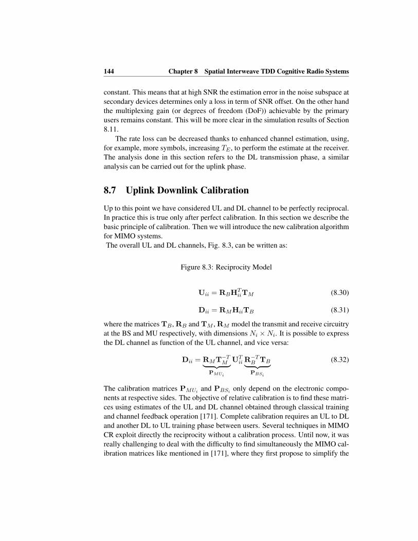
144 Chapter 8 Spatial Interweave TDD Cognitive Radio Systems
constant. This means that at high SNR the estimation error in the noise subspace at
secondary devices determines only a loss in term of SNR offset. On the other hand
the multiplexing gain (or degrees of freedom (DoF)) achievable by the primary
users remains constant. This will be more clear in the simulation results of Section
8.11.
The rate loss can be decreased thanks to enhanced channel estimation, using,
for example, more symbols, increasing TE , to perform the estimate at the receiver.
The analysis done in this section refers to the DL transmission phase, a similar
analysis can be carried out for the uplink phase.
8.7 Uplink Downlink Calibration
Up to this point we have considered UL and DL channel to be perfectly reciprocal.
In practice this is true only after perfect calibration. In this section we describe the
basic principle of calibration. Then we will introduce the new calibration algorithm
for MIMO systems.
The overall UL and DL channels, Fig. 8.3, can be written as:
Figure 8.3: Reciprocity Model
Uii = RBHTiiTM (8.30)
Dii = RMHiiTB (8.31)
where the matrices TB , RB and TM , RM model the transmit and receive circuitry
at the BS and MU respectively, with dimensions Ni ×Ni. It is possible to express
the DL channel as function of the UL channel, and vice versa:
Dii = RMT−TM︸ ︷︷ ︸
PMUi
UTii R
−TB TB︸ ︷︷ ︸PBSi
(8.32)
The calibration matrices PMUi and PBSi only depend on the electronic compo-
nents at respective sides. The objective of relative calibration is to find these matri-
ces using estimates of the UL and DL channel obtained through classical training
and channel feedback operation [171]. Complete calibration requires an UL to DL
and another DL to UL training phase between users. Several techniques in MIMO
CR exploit directly the reciprocity without a calibration process. Until now, it was
really challenging to deal with the difficulty to find simultaneously the MIMO cal-
ibration matrices like mentioned in [171], where they first propose to simplify the

8.8 Beamforming Design with Channel Calibration 145
problem, in subdividing the MIMO channel into Ni×Nj single channels calibrated
separately. However, this solution fails compensate the antenna coupling effects
since it assumes that the calibration matrices are diagonal [173]. Therefore, they
propose an iterative method where each calibration matrix is found alternatively,
but the convergence of this technique has not been proved yet. In the sequel, we
will describe a technique to find simultaneously the MIMO calibration matrices.
In our study, according to the relative calibration principle the question is:
”How to calibrate the cross links in a CR system where communication between
primary and secondary systems is not allowed?”. As we shall see in the following
despite the stringent secondary beamformer requirement (the interference should
lie in the crosslink Rx noise subspace) no calibration is required between crosslink
Tx-Rx devices. This result is a key element to implement spatial interweave CR
systems.
It must be noted that in our CR scenario, the calibration phase of secondary link
will interfere a little with the primary link (and vice versa) but considering that the
training phase for calibration is infrequent, the interference caused is negligible.
8.8 Beamforming Design with Channel Calibration
8.8.1 Primary Beamformer Design
In this section we will discuss how the calibration of Tx-Rx electronics can be
incorporated in the beamformer design.
BS1 performs an SVD decomposition of the UL channel U11 = ZDWH that
it estimates directly using pilots transmitted by MU1. The primary DL channel can
be written as function of the UL channel SVD decomposition using the calibration
filters as:
D11 = PMU1UT11PBS1 = PMU1W
∗DZTPBS1 (8.33)
in order to diagonalize the DL channel BS1 designs its beamformer subspace as
TBS1 = P−1BS1
Z∗, and hence the receiver filter at MU1 is given by: RMU1 =
WTP−1MU1
.
During UL transmission it is possible to design the transmit and receive filters
using the UL channel as reference. In doing so, calibration filters do not appear in
the expression and thus the transmit matrix at MU1 is TMU1 = W and the receive
filter at BS1 is: RBS1 = ZH .

146 Chapter 8 Spatial Interweave TDD Cognitive Radio Systems
8.8.2 Secondary Beamformer Design
The signal at secondary BS due to primary and secondary Tx is expressed as
y2 = U21TMU1s1 +U22TMU2s2 + n2 (8.34)
Knowing U22TMU2 estimated through MU2 beamformed pilots, BS2 can deter-
mine the MU1 Tx subspace U21W using second order statistics.
Now let us consider the signal at MU1, after the Rx filter, which is given by
r1 = RMU1D11TBS1s1︸ ︷︷ ︸r1,s
+RMU1D12TBS2s2︸ ︷︷ ︸r1,int
+n1 (8.35)
where r1,s represents the useful signal part and r1,int contains the interference term.
The objective of the secondary user is to transmit without causing any interference
to the primary system. So BS2 must design its beamformer subspace such that
r1,int = 0. Expressing the DL channel D12 as function of the UL channel and the
calibration filters we can write
r1,int = RMU1D12TBS2s2 = WTUT21PBS2TBS2s2 (8.36)
because BS2 knows the calibration filter PBS2 it is possible to parameterize TBS2 =P−1
BS2TBS2 , so it is possible to design the beamformer subspace, in order to cause
zero interference at MU1 after its receiver filter, as
TBS2 ⊆ (WTUT21)
⊥ (8.37)
Similar treatment applies to the design of MU2 beamformer which are not dis-
cussed here.
It is important to remark that the secondary transmitter can design the beam-
former subspace using only its own calibration factor, obtained during the calibra-
tion phase only with its intended receiver. Then the UL channel and the receiver
subspace at MU1 are estimated using second order statistics of the received signal.
Calibration with non cooperative users is not required.
8.9 Practical Considerations in Spatial IW CR
Despite a pragmatic approach taken in this work to spatial interweave CR design,
we nevertheless make a strong assumption, namely the Tx/Rx subspace is the same
in the primary system. In practical system, this condition may not be satisfied for
several reasons, for example a different ratio of power constraint and noise vari-
ance between the BS1 and MU1 may lead to different number of streams in UL

8.10 Extension to multiple Primary pairs 147
and DL. One subspace will be the subset of the other. A more drastic difference
could be the presence at one end of colored noise instead of white noise or differ-
ent colored noises at the two ends in which case whitened channels may lead to
unrelated Tx/Rx subspaces. In such cases, secondary systems can resort to zero-
forcing beamforming on the crosslink if enough degrees of freedom are available.
This implies a smaller number of secondary Tx streams but the IW paradigm is
still satisfied.
If the primary link is affected by colored noise due to secondary link leakage,
one may observe that the CR is no longer strictly spatial interweave and fits the
underlay paradigm [58]. When this happens, TDD is not enough to design Tx/Rx
filters and feedback is also required between BS1 and MU1. Furthermore, estima-
tion of interference plus noise covariance matrices is needed for channel whitening
and primary beamformer design. In some way, the CR problem starts resembling
a classical MIMO interference channel.
8.10 Extension to multiple Primary pairs
The system model described so far can be easily extended to the situation where a
cognitive system wants to coexist with a set of K primary transmitter and receiver
pairs, Fig. 8.4. This problem formulation depicts the scenario where a femto-cell
is deployed at the cell edge of a macro cell, thus the femto communication suffers
from the interference received from the surrounding macro-cells. The primary sys-
Figure 8.4: Setting with multiple primary pairs
tem can be interpreted as a K-user MIMO interference channel (IFC). To mitigate
the interference that each macro user receives from the other macro transmissions
we assume that an interference alignment transmission strategy is used at the level
of macro communication. This strategy has been shown to maximize the degrees
of freedom for the K-user MIMO IFC [28]. In this section we generalize the sys-
tem model assuming that the k-th primary BS is equipped with Mk antennas while
the corresponding primary MU has Nk antennas and they want to exchange dkstreams. We denote the number of antennas at secondary BS and MU as Ms, Ns
respectively. To simplify the notation we define with Gl and Fl the transmit and
receive filter matrices at primary pair number l and with Gs and Fs the same quan-
tities at the secondary pair. As discussed in chapter 3 the transmit beamformers are
designed such that the interference caused by all transmitters at each non-intended
Rx lies in a common interference subspace. Then with a ZF receiver the interfer-
ence can be completely suppressed. The interference alignment conditions can be

148 Chapter 8 Spatial Interweave TDD Cognitive Radio Systems
simply described as:
FkHklGl = 0 ∀l 6= k (8.38)
rank(FkHkkGk) = dk ∀k ∈ {1, 2, . . . ,K} (8.39)
This last rank condition leads to the traditional single user MIMO constraint dk ≤min(Mk, Nk) for dk streams to be able to pass over the k-th link. Since we suppose
to use a TDD communication protocol thanks to channel reciprocity IA duality still
holds, then :
FkHklGl = 0 ∀l 6= k (8.40)
rank(FkHkkGk) = dk ∀k ∈ {1, 2, . . . ,K} (8.41)
where Fl = GHl , Gl = FH
l are the UL-DL relationship between transmit and
receive filters. From this conditions we can see that, as in the previous case with
one single primary pair, the transmit signal subspace corresponds to the receive
signal subspace.
The signal at the output of the k-th primary MU can be written as:
rk = FkHkkGksk +∑
l 6=k
FkHklGlsl + FkHksGsss + Fknk
= FkHkkGksk + FkHksGsss + n′
k
where we denoted with Hks the channel matrix between the secondary BS and the
k-th primary MU and with n′
k the noise at the output of the receive filter.
The stated objective of our investigation is to design the transmit filter at the sec-
ondary network such that the interference generated at all primary receivers is zero:
FkHksGs = 0, ∀k. The received signal at cognitive BS in the UL transmission
phase can be written as:
ys = HssGsss +K∑
l=1
HskGksk + ns (8.42)
As shown in section 8.4.2 and 8.4.3 from the received signal at the secondary BS
we can estimate the primary signal subspace generated at the secondary BS using
semi-blind subspace estimation. Due to channel reciprocity and duality of IA the
Tx and Rx signal subspace at each primary device are the same:
HI =[Hs1G1, . . . ,HsKGK
]=
F1H1s...
FKHKs
H
= HHI
8.10 Extension to multiple Primary pairs 149
HI is the composite secondary to primary channel as seen at the joint outputs of the
primary UEs. Then the signal subspace at all primary MUs in the DL communica-
tion, spanned by HI , can be estimated from the received signal at the secondary BS
(8.42), using semi-blind techniques. The knowledge of the primary Tx subspace is
enough to design the Tx filter at the secondary BS such that the interference that
the secondary communication generates at each primary receiver lies in the noise
subspace. This implies:
HIGs = 0 =⇒ Gs ⊆ span(HHI )⊥
The last relationship says that the BF chosen by the secondary BS should be in the
orthogonal complement of the subspace spanned by the matrix HI In order to have
a possibility to design the Tx filter each cognitive device should be equipped with
a number of antenna greater than the total number of streams transmitted in the
primary network: Ns,Ms >∑K
k dk.
8.10.1 Transmit and receive filter design with calibration filters
In this section we show how to design the IA filters for the primary network and
the transmit and receive filter at the cognitive users when calibration filters need to
be included in the filter design.
Initially we consider the IA design at the primary network.
Primary BSs and MUs, with the estimate of the UL channels, calculate the
transmit and receive filters for the UL transmission using an iterative algorithm
available in literature, for example [34] or [33]. Then the UL IA conditions are
satisfied:
FkUklGl = 0.
To apply the UL filters in the DL communication each terminal should pre-compensate
for the UL-DL channel mismatch, as done in section 8.8:
Gk = P−1BSk
FTk
Fl = GTl P
−1MUl
(8.43)
Applying the IA filter, found above, in the DL transmission we get:
FlDlkGk = FlPMUlUT
klPBSkGk = G
Tl U
TklF
Tk = (FkUklGl)
T = 0
then the IA conditions also in the DL are satisfied. This concludes the filter design
in the primary network. To understand how the secondary network can find the
150 Chapter 8 Spatial Interweave TDD Cognitive Radio Systems
BF matrices for the concurrent transmission we fist study the received signal at the
secondary BS in the UL transmission:
ys = UssGsss +
K∑
l=1
UskGksk + ns (8.44)
from the received signal above, the subspace spanned by the matrix
HI =[Us1G1, . . . ,UsKGK
]can be estimated. The objective of the secondary
BF design is to cause zero interference at all the primary receivers, then the inter-
ference contribution at, for example, primary MUk can be written as:
rk,int = FkDksGss2 = GTkU
TskPBSsGss2. (8.45)
We parameterize the BF at the secondary BS as Gs = P−1BSs
Gs because BSs
knows the calibration filters obtained during the secondary calibration phase, then
the secondary BF subspace can be designed such that (UskGk)T Gs = 0, ∀k,
then we choose:
Gs ⊆ span(HTI )
⊥
In this section we have shown that it is possible to extend the results obtained for
spatial interweave in the simple scenario of one primary and secondary pair also
to the case of multiple primary users when the transmit and receiver filter design
of the primary system is IA. Here we have proved that also in this setting the
calibration between primary and secondary users is not required for the calculation
of the secondary transmitters. A sub-product of this analysis is that also to find
an IA solution, in the pure MIMO IFC, using UL-DL duality each device only
needs its own calibration coefficient, so calibration between pairs of primary users
is also not required. This is another important remark because if we want to exploit
channel reciprocity also for IA design we have shown that calibration is necessary
and this must be done only between users of the same pair.
8.11 Numerical Results
Figure 8.5: Rate Comparisons
Fig. 8.5 depicts the rate curves for the primary and secondary links. We com-
pare the performances of a cognitive radio system where the licensed users have
N1 = 4 transmitting and receiving antennas. We report in the same figure the
rate performances of a secondary system that have two possible antenna config-
urations: N2 = 4 and N2 = 7. The primary communication is not affected by

8.11 Numerical Results 151
the opportunistic transmission thanks to the proper beamformer design of the sec-
ondary devices. On the other hand the rate of the secondary is very dependent of
the number of antennas. The plot shows that if the secondary users have the same
number of antennas of the primary the transmission takes place only in the low
SNR region because the opportunistic users can only communicate using unused
modes of the primary communication. When licensed users use all the possible
modes there is no room for secondary transmission and hence the rate curve goes
to zero. Different is the situation of an opportunistic user that is equipped with
more antennas than the licensed one. In this case the cognitive user can transmit in
all SNR regimes. In particular at high SNR the secondary system is able to sustain
a significant rate.
In Fig. 8.6 we report the rate curves of a cognitive system where the licensed
users have N1 = 1 antenna and the secondary transmitter and receiver have N2 = 9antennas. Here we want to study the effect of differential feedback on the sec-
ondary transmission. As we can see having imperfect CSIT deteriorates the per-
formances. In particular we can see that increasing the number of iteration for
the feedback acquisition corresponds to an increases of the CSIT quality and this
reflects into an increase of performances. For both number of feedback iterations
that we consider, ITERFB = {5, 10}, there is a loss in term of multiplexing gain
achieved by the secondary users. This is revealed from the loss in slope of the
two red curves compared to the green one that represents the perfect CSIT case.
Usually for digital feedback in order not to loose in multiplexing gain the number
of bits used for feedback transmission should increase with the SNR. Here we see
that to obtain the same effect the number of iterations should increase as the SNR
increases. A different transmit strategy could be used, like analog feedback, that
does not require iterations but only the transmission of un-quantized channel coef-
ficients.
Finally we want to study the effect of estimation error in the blind subspace es-
Figure 8.6: Rate comparisons with feedback
timation procedure at the secondary transmitters. In Fig. 8.7 we report the rate
curves achieved by the primary user with and without error in the subspace esti-
mation procedure at the secondary user. We can notice that if an error is present
then the beamforming design at the secondary is not perfect and hence a residual
interference is present in the primary signal. In figure 8.7 we also compare the rate
at the primary user when different number of samples TE is used in the subspace
estimation procedure. As we were expecting the longest the estimation period is
the better the estimate is, hence the rate loss decreases. We can also see that the rate
loss due to signal subspace estimation affects only the SNR offset and not the mul-
152 Chapter 8 Spatial Interweave TDD Cognitive Radio Systems
tiplexing gain. This can be seen comparing the slopes of the three curves. In Fig.
Figure 8.7: Rate comparisons with estimation error at the secondary transmitter
8.8 we compare the theoretical rate loss, ∆Rtheo upper bound found in section 8.6,
with the experimental one ∆Rexp. As we can see the upper bound that we found
becomes tighter as the number of samples TE used for the estimation procedure
increases. The rate loss is not constant over the SNR because it also depends on
the number of transmitted streams d1, so it increases with the increase of d1. When
the primary transmitter uses all the available modes then ∆R remains constant.
Figure 8.8: Rate loss comparisons
8.12 Conclusions
We addressed the beamformer design for a secondary communication system in
a spatial interweave CR system. The practical problem of opportunistic CSI ac-
quisition was addressed by exploiting primary signal statistics and reciprocity of
the underlying TDD channel. Beamformer for secondary Tx is designed so that
the secondary signal lies in the noise subspace of the primary signal. It must be
noted that spatial interweaving of secondary’s signal with the primary’s relies on
reciprocity of the TDD channel. Tx/Rx calibration is therefore mandatory.
The main contribution of this chapter is the discovery that despite the require-
ment for channel reciprocity between noncoperative users, calibration between
crosslinks is not required. We also extended the results to a CR system where a
single secondary pair coexists with multiple primary user organized as an interfer-
ence channel.

Chapter 9
Spatial Interweave Cognitive
Radio Interference Channel with
Multiple Primaries
9.1 Introduction and state of the art
In the previous chapter we have introduce the concept of Spatial Interweave where
exploiting the unused spatial dimensions of the primary system we can setup an op-
portunistic communication. In this chapter we further exploit the spatial dimension
in the interweave paradigm considering a secondary network modeled as a MIMO
interference channel, with multiple transmit-receive pairs, and where the BF ma-
trices are designed according to IA among secondary users while constraining the
interference caused to the primary receiver to be in a subspace of reduced dimen-
sions. A similar setting, but with only one pair of primary and secondary users, was
considered in [169]. In [180] the authors extended the setting in [169] to multiple
secondary pairs but constraining the number of primary users to only one pair of
transmit-receive terminals, each transmitter is a single antenna device while all the
receivers are equipped with multiple antennas. For this setting the authors intro-
duced the concept of Opportunistic Spatial Orthogonalization (OSO) that allows
the coexistence of multiple secondary pairs and primary users. The idea is based
on a selection process, done at the primary receiver, that selects the secondary pair
that interfere the least with the primary communication. This concept relies on the
153

154Chapter 9 Spatial Interweave Cognitive Radio Interference Channel with Multiple Primaries
randomness and independence of the channel vectors to take advantage of the mul-
tiuser diversity. The authors of [181] also extend the setting in [169] to multiple
secondary pairs with only one pair of primary transmit-receive terminals consid-
ering multi antenna terminals at both ends. Extending the results on IA feasibility
in [37] they provide a condition for IA feasibility in the described CR setting. In
addition an iterative algorithm, for secondary users’s beamformer design is intro-
duced. A similar setting was studied in [182] where the secondary network, model
as an interference channel, coexists with a single primary users using an IA trans-
mission strategy. Two settings are considered: SISO and MIMO. For the SISO
case an IA solution based on symbol extension is introduced while for the MIMO
case an iterative algorithm, based on gradient method, is used for the secondary
users’ beamformer design. In [183] a MIMO interference channel is considered as
primary network where IA transmission strategy is used to exchange useful data.
At the same time a set of secondary multi-antenna users desire to access to the pri-
mary network and this can be done only if the primary users’ transmission is not
modified. The authors present a condition for user admission and a set of beam-
forming design solutions for the secondary users with the objective of maximizing
the secondary users’ rate.
9.2 Contributions
In our work we consider an arbitrary number of secondary users pair that want to
set up a communication in presence of L primary multi antenna receivers. The
secondary network applies IA beamforming strategy constraining the interference
subspace, generated at each primary receiver, to have a given dimension. With the
cognitive constraint the correct number of primary users’ streams can be retrieve
at the primary receivers. We study the feasibility of an IA solution of the cognitive
radio system under investigation based on the results presented in chapter 3. The
solution obtained takes also into account the additional cognitive constraints that
allow the secondary interweave communications. In addition we introduce an iter-
ative algorithm that allows us to design the secondary users’ transmit and receive
filters. Introducing a fictitious zero forcing receive filter at each primary receiver
we rewrite the rank constraints, on the interference subspace at the primary user, as
an additional set of IA constraints. This allows us to extend the algorithm proposed
in [33] to the proposed cognitive radio setting.

9.3 Signal Model 155
9.3 Signal Model
The cognitive radio setting that we consider in this chapter is depicted in Fig. 11.1.
The system setting that we study can be used to model the coexistence of a set Kof femto-cells with the presence of L macro-users.
Figure 9.1: Cognitive Radio System
The secondary network is a K-link MIMO interference channel with K transmitter-
receiver pairs. To differentiate the two transmitting and receiving devices we as-
sume that each of the K pairs is composed of a secondary Base station (SBS) and a
secondary Mobile user (SMU). This is only for notational purposes. The k-th SBS
and its corresponding SMU are equipped with Mk and Nk antennas respectively.
The k-th transmitter generates interference at all l 6= k receivers. The received
signal yk at the k-th SMU, can be represented as
yk = Hkkxk +K∑
l=1l 6=k
Hklxl + nk (9.1)
where Hkl ∈ CNk×Ml represents the channel matrix between the l-th SBS and
k-th SMU, xk is the CMk×1 transmit signal vector of the k-th SBS and the CNk×1
vector nk represents (temporally white) AWGN with zero mean and covariance
matrix Rnknk. The channel is assumed to follow a block-fading model having a
coherence time of T symbol intervals without channel variation. Each entry of the
channel matrix is a complex random variable drawn from a continuous distribution.
It is assumed that each transmitter has complete knowledge of all channel matrices.
We denote by Gk, the CMk×dk precoding matrix of the k-th transmitter. Thus
xk = Gksk, where sk is a dk × 1 vector representing the dk independent symbol
streams for the k-th user pair. We assume sk to have a spatio-temporally white
Gaussian distribution with zero mean and unit variance, sk ∼ N(0, Idk). The k-th
receiver applies Fk ∈ Cdk×Nk to suppress interference and retrieve its dk desired
streams. The output of such a receive filter is then given by
rk = FkHkkGksk +K∑
l=1l 6=k
FkHklGlsl + Fknk
In this work we design the Tx and Rx filter matrix at the cognitive receiver accord-
ing to interference alignment (IA). For more details on IA and the corresponding

156Chapter 9 Spatial Interweave Cognitive Radio Interference Channel with Multiple Primaries
IA conditions please refer to chapter 3 and [28]. The secondary network wants to
coexist with a set of L multi antenna primary mobile users (PMU). To simplify
the notation we index the L PMUs from K + 1 to K + L. With this notation
the channel matrix between the SBSk and the PMUK+l is denoted HK+lk and
has dimensions NK+l × Mk, where NK+l represents the number of antennas at
PMU number l. The receiver filter applied at the PMUK+l is denotes as FK+l,
in this chapter we do not consider the optimization of the primary transmission so
the receiver FK+l is a general receiver. We only assume it involves a fixed num-
ber of transmitted stream dK+l. In the following we consider the situation where
the primary transmitter (PBS) is located far from the secondary system and hence
no interference is caused to the secondary network from the primary communica-
tion. We constraint our attention to the scenario where each primary receiver has
to suppress only the interference coming from the secondary network. Primary
user receiver design is not considered here. In this chapter we do not make any
assumption on the antenna configuration at the primary and secondary network
but we should underline that two possible situations can occur. In particular if the
number of antennas in the secondary network is grater that the number of antennas
at the primary users then blind channel estimation is possible. On the other hand
if the secondary network has less antennas than the primary users then the primary
training signal should be explored for the channel estimation process.
9.4 Interference Alignment for Cognitive Radio System
In this section we specify the IA conditions, presented in chapter 3, for the cog-
nitive radio system that we consider in this work. As explained before the focus
of our work is to design a set of K IA beamformers and receiver filters such that
the interference at each primary MU is constrained in the subspace of fixed dimen-
sions. This means that on top of the usual IA conditions we need to impose the
additional interweave constraints:
FHk HklGl = 0 ∀l 6= k (9.2)
rank(FHk HkkGk) = dk ∀k ∈ {1, 2, . . . ,K} (9.3)
rank
[K∑
k=1
HK+lkGk
]≤ NK+l − dK+l ∀l = 1, . . . , L (9.4)
The rank requirements at the primary receiver described above can be interpreted
in an alternative way. If we assume that each PMU applies a fictitious interfer-
ence suppressing filter FK+l such that it retrieves dK+l interference free streams,

9.4 Interference Alignment for Cognitive Radio System 157
condition (9.4) reads:
FK+l
[K∑
k=1
HK+lkGk
]= 0 ∀l = 1, . . . , L (9.5)
This condition says that the Interference Leakage [33] at each PMU should be equal
to zero. The receiver FK+l is introduced only for the derivation of an iterative
algorithm it is not the real receiver applied at the PMUs. With this modification
we can interpret the entire network as an asymmetric IFC with K transmitters and
K + L receivers. Using the results proposed in [33] we can extend their algorithm
to the CR setting that we consider here.
The objective of the algorithm is to find a set of BF and Rx filters such the the
leakage interference at each receiver is minimized. If an interference alignment
solution exists the residual interference will be completely suppressed.
The interference leakage at receiver k is defined as:
ILk = Tr[FkRkF
Hk
]∀k = 1, . . . ,K + L
where the interference covariance matrix at receiver k is defined as
Rk =
K∑
l 6=k
Pl
dl
HklGlGHl H
Hkl, k = 1, . . . ,K
K∑
l=1
Pl
dl
HklGlGHl H
Hkl, k = K + 1, . . . ,K + L
Pl represents the Tx power for user l. The algorithm to determine the Tx and Rx
filters is based on Reciprocity of IA solutions [33]. It iterates between the original
and the reciprocal system. The reciprocal network can be the real dual system or a
fictitious network used only in the BF design algorithm. In our case the reciprocal,
dual network, is described by a dual channel Hkl = HHlk, the reciprocal Tx and Rx
filters are Fk = GHk , Gk = FH
k . With those definitions the leakage interference in
the reciprocal network is:
ILk = Tr[FkRkF
H
k
]∀k = 1, . . . ,K (9.6)
where the dual interference covariance matrix is defined as:
Rk =
K+L∑
l 6=k
Pl
dl
HklGlGH
l HHkl (9.7)

158Chapter 9 Spatial Interweave Cognitive Radio Interference Channel with Multiple Primaries
as we can see from the definitions above there is a difference between original and
reciprocal network due to the non symmetric structure of our system. As described
in [33] to find the Tx and Rx filters we need to minimize the leakage interference in
the original and reciprocal system in particular for all k = 1, . . . ,K + L we have
to solve the following:
minFkF
Hk =I
ILk ∀k = 1 . . . ,K + L (9.8)
The optimal solution of this problem is given by the eigenvectors of Rk corre-
sponding to the dk smallest eigenvalues. In a second step we solve the same prob-
lem but for the reciprocal UL system, determining the UL Rx filters at SBSk for
k = 1, . . . ,K. The solution is obtained solving, as done for the DL problem, the
following UL problem:
minFkF
Hk =I
ILk ∀k = 1 . . . ,K (9.9)
Algorithm 7 Iterative Algorithm for Cognitive IA
Fix the initial set of precoding matrices Gk, ∀ ∈ k = {1, 2 . . .K}repeat
Find Fk k = 1 : K + L as the dk eigenvector corresponding to the smallest
eigenvalue of Rk
Reverse the system and solve in the reciprocal system
until convergence
9.5 Interference Alignment Feasibility
To determine the existence of an IA solution for a given DoF allocation in our CR
scenario we the translate the IA equations into a set of conditions that need to be
satisfied to admit an IA solution.
FkHklGl = 0 ∀l 6= k (9.10)
rank(FkHkkGk) = dk ∀k ∈ {1, 2, . . . ,K} (9.11)
rank
[K∑
k=1
HK+lkGk
]≤ NK+l − dK+l ∀l = 1, . . . , L (9.12)
The approach we adopt in this chapter is of formulating the given IA problem
as finding a solution to a system of equations with limited number of variables
9.5 Interference Alignment Feasibility 159
dictated by the dimensions of the overall system. The interference aligning beam-
former matrix Gk aligns the transmit signal of the k-th user to the interference
subspace at all l 6= k users while ensuring the rank of the equivalent channel ma-
trix FkHkkGk is dk. The only requirement on the (dk × dk) matrix that mixes up
the desired streams is that it be of full rank. The beamforming matrix is defined up
to an arbitrary (dk × dk) square matrix. Thus, of the total number of (Mk × dk)variables available for the design of Gk matrix reduces to dk(Mk − dk).Considering all the SBS the total number of variable available at the Tx side is:
K∑
i=1
di(Mi − di) (9.13)
The IA scheme essentially requires that all alignment is done at the Tx. Therefore
every Tx imposes a set of constraints on the entire system whenever it transmits
a stream to its Rx. An IA solution will be feasible only if the total number of
variables available in the system is greater than or equal to the total number of con-
straints to be satisfied. Moreover, the variables should be distributed appropriately
at each of the Tx. Here we propose a method of counting the number of variables
available for the design of beamformers and comparing them with the number of
constraints imposed on the system.
The main idea behind our method is to convert the alignment requirements at each
Rx into a rank condition of an associated interference matrix.
Because in our CR system we have a set of additional requirements for the align-
ment at the primary receiver we have to consider also the interference matrix that
the secondary transmissions span at each PMU. For this reason we first study the
problem of the alignment at the secondary network and then we consider the pri-
mary constraints.
At SMU k, the interference due to all other (K − 1) secondary transmitters is
grouped into a (Nk ×∑K
l=1;l 6=k dl) matrix
H[k]IS=[Hk1G1, ...Hk(k−1)G(k−1),Hk(k+1)G(k+1), ...HkkGK ],
that spans the interference subspace. The total signal-space dimension at SMU
k is given by the total number of receive antennas Nk and dk are to be reserved
for the signal from the k-th PBS. This is achieved when the interference from all
other transmitters lies in an independent subspace whose dimension can be at most
(Nk − dk). Thus the dimension of the subspace spanned by the matrix H[k]IS must
satisfy
rank(H[k]IS ) = r[k]
IS ≤ Nk − dk (9.14)

160Chapter 9 Spatial Interweave Cognitive Radio Interference Channel with Multiple Primaries
Imposing a rank r[k]IS on H
[k]IS implies imposing
(Nk − r[k]IS)(
K∑
l=1l 6=k
dl − r[k]IS)
constraints at Rx k. In general the rank r[k]IS should satisfy the following upper
bound
r[k]IS ≤ min(dtot, Nk)− dk (9.15)
where dtot =∑K
k=1 dk.
At PMU K + l the interference coming from the entire secondary network can
be identified with an interference matrix of dimensions (NK+l × dtot):
H[K+l]IP =[HK+l1G1, . . . ,HK+lKGK ].
To satisfy the CR constraint the interference matrix H[K+l]IP should span a subspace
of dimensions
rank(H[K+l]IP ) = r[k]
IP ≤ NK+l − dK+l. (9.16)
According to the rank requirement and the dimensions of the interference matrix
H[K+l]IP satisfies the following upper bound:
r[K+l]IP ≤ min(dtot, NK+l − dK+l) (9.17)
Imposing a rank constraint (9.12) on the interference matrix at the PMU implies
imposing
(NK+l − r[K+l]IP )(dtot − r[K+l]
IP )
constraints. Once we know how to calculate the number of variable available to
design the IA precoding matrices and the number of constraints that the IA solution
imposes on the system under investigation we can write the final relation in (9.19).
To evaluate the existence on an IA solution it is not only important that the
number of variable is enough to satisfy the constraints that the IA imposes on our
system but we should study also how this variables are distributed among all the
users. To consider this aspect we propose a recursive procedure based on study-
ing IA feasibility on a subsystem built by successively adding one transmitter at a
time [184]. At each step k of the recursion, (9.19) accumulates the total number
of variables available for designing an IA solution in an associated sub-problem
comprising of a k-link MIMO IFC in the LHS of (9.19), where dk =∑k
i=1 di. In
the considered subproblem only k transmitters are transmitting non-zero streams

9.6 Simulation Results 161
and aligning their streams into some interference subspace of all non-intended re-
ceivers. The RHS accumulates the total number of constraints at all receivers that
arise due to these transmitters.
Consider a network where the secondary system is symmetric hence Mk =Nk = NS, dk = dS ∀k = 1, . . . ,K and a primary system with NK+l = NP , dK+l =dP ∀l = 1, . . . , L. In this particular scenario we can specify a condition that the
antenna distribution in the secondary network should attain to obtain the desired
stream allocation satisfying, at the same time, the rank requirement at the PMU.
Neglecting trivial cases as NP > KdS and NS > KdS we can specify condition
(9.19) as follows:
NS ≥ K + 1
2dS +
LdP
2KdS
(KdS − (NP − dP )) (9.18)
From the condition above we can see that compared to the simple K-users MIMO
IFC introducing a set of primary user interference constraint causes a reduction in
terms of performances. In particular to obtain the same DoF of a traditional MIMO
IFC additional LdP2KdS
(KdS − (NP − dP )) antennas are required in order to handle
the interference to the primary users. If equation (9.18) is derived for the case
where the PMU does not have any noise subspace ((NP − dP )) our conditions for
symmetric systems becomes similar to the equivalent condition given in [181].
k∑
i=1
di(Mi − di) ≥k∑
i=1
(Ni − (min(dk, Ni)− di)︸ ︷︷ ︸r[i]IS
)(dk −min(dk, Ni))
+K∑
i=k+1
(Ni −min(dk, (Ni − di))︸ ︷︷ ︸r[i]IS
)(dk −min(dk, (Ni − di)))
+
K+L∑
i=K+1
(Ni −min(dk, (Ni − di))︸ ︷︷ ︸r[i]IP
)( dk −min(dk, (Ni − di)))
(9.19)
9.6 Simulation Results
Figure 9.2: Sum rate performances

162Chapter 9 Spatial Interweave Cognitive Radio Interference Channel with Multiple Primaries
In this section we present some simulation results for the cognitive radio sce-
nario that we presented. In Fig. 9.2 we report the sum rate of the primary and
secondary system. In particular there is a single primary receiver with NP = 2antennas. To calculate its rate we assume that it communicates with a primary
transmitter according to a single user MIMO communication without receiving in-
terference from the secondary communication. Thus the the primary Tx and Rx are
built according to water filling like technique. In high SNR regime this will lead to
a maximum of dP = 2 transmitting streams. The secondary network is modeled
as a K = 2 MIMO IFC where each secondary pairs wants to send dk = dS = 1stream each. To satisfy interference alignment requirements and the interference
rank constraints to the primary, according to (9.18), each Tx and Rx pair should be
equipped with Mk = Nk = NS = 3 transmitting and receiving antennas.
As we can the two curves are parallel in the high SNR regime. This means that the
secondary network is able to achieve the same DoF of the primary network hence
the total required number of streams has been sent. The rate curve of the secondary
system is characterized by an higher SNR offset, this is due to the higher number
of antennas of the cognitive devices compare to the primary users that determines
an antenna gain.
9.7 Conclusions
We address the problem of BF design in the CR system where the secondary net-
work is a K-user MIMO IFC. At the same time a set of L multi-antenna primary
receivers are affected by the interference generated from the SBS transmitted sig-
nals. The objective of our investigation is to design IA BF for the secondary net-
work constraining the interference to the primary receiver to span a subspace of
proper dimensions. To accomplish this objective we propose an iterative algo-
rithm. In addition we present a set of IA feasibility conditions that if not satisfied
immediately rule out the possibility of designing such cognitive IA beamformers.

Chapter 10
Conclusions
In this thesis we mainly tackled the transmit and receive filter design for different
interfering systems: interference and cognitive radio channels.
In the first part we were mainly interested in studying the interference channel
with particular focus on multi antenna systems. We first studied the beamforming
problem in a MISO interference channel. Then we moved to the more complex
problem of joint transmit and receive filter design in MIMO interference channel.
Interference alignment and weighted sum rate approach were considered. Those
approaches rely on full CSIT and CSIR that in more realistic scenarios is difficult
to be achieved. We then focus on a robust approach to design optimal transmit
beamformers when stochastic CSI is available at the transmit side. Finally we pro-
posed two transmission protocols to achieve the required channel state information
at both ends with the consequent optimization of the number of transmitted streams
as function of the coherence time.
In the second part of the thesis the cognitive radio channel was studied. In
particular we first studied the beamforming problem for a MISO underlay cogni-
tive interference channel and then we introduced the concept of spatial interweave.
There transmitters and receivers, at the secondary network, were jointly optimized
to cause zero interference to the primary receivers. The proposed solutions rely on
the spatial dimensions to control the interference generated to primary users.
In the following we give the conclusions and the corresponding future extensions
of the main themes treated in this thesis.
• Beamforming in the MISO Interference Channel
163

164 Chapter 10 Conclusions
We studied the problem of maxmin SINR with minimum QoS constraints
and per-user power constraints for a MISO IFC. We derived an iterative al-
gorithm to solve the problem based on the equivalence between SINR bal-
ancing and the power minimization problem, that allows distributed imple-
mentation. The solution is based on the recent results on UL/DL duality for
IFC. We showed that when the IFC is separable the optimum of the SINR
balancing problem is achieved when all users transmit with full power. On
the other hand if none of the users can apply a ZF beamformer then only one
user transmits with full power. These pieces of information can be used to
develop an algorithmic solution in simplified problems. The interest behind
the weighted SINR balancing problem resides on the possibility to use its
solutions to characterize the complete Pareto boundary of the SINR (Rate)
region of a MISO IFC.
The natural extension of this work includes the analysis of the MIMO in-
terference channel. There the main difficulty is the definition of QoS con-
straints in multi stream communication. The optimal approach should be to
work with per-receiver rate constraints that can also include joint decoding of
the received streams. This approach is indeed difficult to handle so a possi-
ble suboptimal approach would be to work in a per stream fashion assuming
linear receive filters, that now should also be optimized. The solution of the
maxmin rate problem with per user rate constrains can, in any case, give
some hints in the characterization of the rate region of the general MIMO
interference channel.
• Interference Alignment in the MIMO Interference Channel
We considered the problem of analytically evaluating the feasibility of an
interference alignment solution for a given degrees of freedom allocation in
a general K-link MIMO IFC. We introduced a systematic method to check
the feasibility of an interference alignment solution for a given MIMO IFC.
In addition we also showed that exploring the fact that IA feasibility is un-
changed when the MIMO crosslink channel matrices have a reduced rank,
we propose a new way to study the problem using numerical continuation
method. Finally we observe that using real signal constellations, in place of
complex constellations, transmission over a complex channel can be inter-
preted as transmission over a real channel of double the original dimensions.
This doubling of dimensions provide additional flexibility in achieving the
total DoF available in the network providing a finer granularity in the system
design.
In a recent paper [101] the authors showed that our conditions are only nec-

165
essary and for some particular cases they are not conclusive. Our future
perspectives on this subject include the definition of necessary and sufficient
conditions. This should go in the direction to incorporate, in our test, also
the interaction between interference subspaces generated at non intended re-
ceivers. This, for the moment, is not taken into account since our procedure
is based on counting variables and constraints on a per-receiver basis.
• Weighted Sum Rate maximization in the MIMO Interference Channel
We studied the weighted sum rate maximization for the MIMO IFC introduc-
ing an iterative algorithm to solve this optimization problem. The proposed
solution converges to local optima due to the non-convexity of the MIMO
IFC rate region. To reduce the probability to be trapped in one suboptimal
point we introduced Deterministic Annealing. This approach allows to track
the variation of the known solution of one version of the problem into the
unknown solution of the desired version by a controlled variation of a pa-
rameter called temperature. In our problem the temperature is related to the
inverse of the SNR. From our analysis we introduced a sum rate duality for
the MIMO IFC, where the optimal BF solution resulted to be an MMSE Rx
filter in the dual communication with proper UL Tx covariance matrix and
dual noise variance. The dual of an interference channel is still an interfer-
ence channel so duality does not simplify the solution of the problem. We
can use duality principle to have better interpretation of the provided solu-
tions. We also introduced a more robust version of the WSR algorithm when
stochastic CSIT are available. The proposed approach seems to achieve the
correct DoF distribution in high SNR, if the channel uncertainty scales in-
versely proportional with the SNR.
The problem of WSR maximization is still not solved completely since how
to get a global optimal solution has not been shown. The approach that we
introduced, with deterministic annealing, can give some useful directions. It
is of interest studying analytically the evolution of the cost function at differ-
ent phase splits. This will help to understand how the global optima evolves
as function of the SNR. In addition also some other different approach can
be used in the design an algorithm for WSR maximization. A possible line
of research include approaches in which power and Tx directions are opti-
mized separately. In this way we can have a better handling on DoF alloca-
tion between different users that can probably reduce the occurrence of local
optima.
• CSI Acquisition in the MIMO Interference Channel
The problem of joint transmit and receive filter design, in MIMO IFC, re-

166 Chapter 10 Conclusions
quires full CSI at both side of the communication link. To achieve this
information we analyzed different transmission protocols for the necessary
CSI acquisitions at each BS and MU based on training and analog feedback
transmission. Our final objective was the optimization of the achievable net
degrees of freedom in the network. In particular the time overhead, due to
CSI acquisition, reduce substantially the time left for useful data transmis-
sion. We showed that the optimal number of streams should vary as function
of the channel coherence time. In addition if the coherence time is too short
we showed that, in some condition, SU-MIMO transmission is optimal.
In this chapter we only introduced the problem of DoF optimization as func-
tion of the coherence time. The results provided are given only in some
particular cases in order to simplify the problem formulation. The analysis
for more general antenna distribution should be developed. With these fur-
ther results a more optimal CSI acquisition stage can be design in order to
maximize the total achievable DoF. In addition the recent results on IA with
delayed CSIT (DCSIT) can be included in the analysis to design a more op-
timal communication protocol that uses DCSIT for BF design until full, or
perfect, CSI is achieved with training and feedback.
• Underlay Cognitive MISO Interference Channel
We proposed an iterative algorithm to solve the problem of beamforming
design in MISO cognitive IFC with objective the minimization of the to-
tal transmitted power. In order to meet the underlay requirements we im-
posed a set of interference constraints at each primary receiver. The solution
proposed is based on new results on UL/DL duality for CR channel. The
primary users can be seen as a set virtual primary Txs in the UL commu-
nication, thus supplementary interference links that should be considered in
the secondary Rx design in the UL communication.
The main problem that still need to be solved in this setting is the feasibility
study of the problem. In particular given a set of QoS constraints at the sec-
ondary receiver, per-transmitter power constraints and the set of maximum
interference level tolerated at the primary receivers we should be able to state
if the given problem admits a solution or not. The other natural evolution of
this problem is the extension to a MIMO setting. There the problem defini-
tion is more critical, as explained in the study of the beamforming problem
for traditional MISO interference channel, due to multi stream communica-
tions.
• Spatial Interweave TDD Cognitive Radio Systems
We studied the problem of opportunistic CSI acquisition and secondary beam-

167
former design in a spatial interweave setting posing particular attention to
the practical implementation. We showed that the problem can be solved ex-
ploiting primary signal statistics and reciprocity in TDD communications. In
order to take advantage of channel reciprocity, Tx/Rx calibration is therefore
mandatory.
The main contribution of this chapter is the discovery that despite the re-
quirement for channel reciprocity between non-cooperative users, calibra-
tion between crosslinks is not required. We also extended the results to a
CR system where a single secondary pair coexists with multiple primary
users organized as an interference channel. Also in this case the beamformer
design relies on channel reciprocity. We also showed how IA design is influ-
enced by channel calibration and how the calibration coefficients influence
the Tx/Rx filter design. Then we focused on a different setting in which the
secondary network is organized as a MIMO IFC. There the objective is to
design IA cognitive beamformers constraining the interference subspace di-
mensions to the primary receivers. We developed an iterative algorithm that
solves the problem and we also derived a set of feasibility conditions for IA
design in CR networks.

168 Chapter 10 Conclusions

French Summary
Les systemes traditionnels de communication sans fil sont concus de telle sorte
que la zone de couverture est divisee en zones dites cellules. Dans chaque cel-
lule une station de base (BS) assure la communication pour les utilisateurs qui
se trouvent dans la cellule correspondante. Afin d’eviter ou de reduire les in-
terferences generees par la communication dans les cellules voisines une config-
uration de reutilisation des frequences a ete introduit [2]. Cette approche pour
traiter l’interference empeche la reutilisation d’une ressource spectrale a l’interieur
d’un ensemble de cellules appelees cluster. La reduction d’interference obtenu
avec un facteur de reutilisation de frequence se fait au prix d’une perte d’efficacite
spectrale. Pour cette raison, dans la prochaine generation de cellulaires normes de
communication sans fil, par exemple, Code Division Multiple Access (CDMA), un
facteur de reutilisation de frequence de un a ete utilise.
Facteur de reutilisation de frequence l’un entrane, d’autre part, une reduction dras-
tique de la capacite du reseau en raison de l’augmentation de l’interference. Les
performances des utilisateurs au bord de la cellule sont gravement touches par ce
configuration de reutilisation de frequence agressif en raison de l’augmentation de
l’interference inter-cellules que l’experience de ces utilisateurs. Pour traiter ces
problemes les systemes actuels de communication comprennent differentes solu-
tions de gestion des interferences. Meme si les interferences venant de l’exterieur
de la cellule de transmission peut etre reduit en utilisant une planification minu-
tieuse ou instaurant une cooperation entre cellules voisines, ces techniques ne sont
parfois pas suffisantes pour garantir un debit eleve a utilisateur au bord del la cel-
lule . Pour cette raison, les principaux organismes de normalisation sont main-
tenant y compris les strategies de coordination des interferences dans la prochaine
generation de normes de communication cellulaire. Par exemple, dans les futures
versions de la norme de communication cellulaire appelee Long Term Evolution
Advanced (LTE-A) ces techniques sont regroupees dans ce qu’on appelle emph
Figure 11.1: Cell-edge users problem representation
169
170
Coordinate multipoint transmission et reception [3]. Ces techniques sont fondees
sur la cooperation des stationes de base plus conscient d’interferences.
Les evolutions les plus recentes de cette particuliere technique de communica-
tion cooperative est ce qu’on appelle Network ou Virtual MIMO (Multiple-Input
Multiple-Output), o le concept principal est d’introduire une collaboration plus
etroite entre les stations de base voisines telles que chaque utilisateur est desservi
par plusieurs stations de base. Ce scenario peut etre considere comme un systeme
MIMO broadcast (BC) distribue. Pour l’introduction complete sur les resultats
recents sur ce sujet s’il vous plat se referer a [4]. Pour parvenir a ce resultat
tout le BS doit etre connecte a un systeme centralise de traitement/contrle parce
que la pleine cooperation au niveau de signal est necessaire, en particulier toutes
les stations de base doivent etre conscients de tous les messages destines a tous
les utilisateurs du reseau. Ces techniques de cooperation, dans leur mise en uvre
dans LTE-A, se sont reveles apporter une amelioration significative de l’efficacite
spectrale pour les utilisateurs au bord de la cellule, tandis que le gain resultant
de la couverture cellulaire complete est presque negligeable [5]. Bien que tres
utile, au moins pour ameliorer la performance de la cellule de pointe utilisateurs,
ces techniques presenter quelques difficultes dans les systemes reels. Realiser le
necessaire collaboration et la coordination entre les differentes stations de base
pose des problemes differents dans des systemes reels avec une capacite backhaul
limitee et une latence finie.
11.1 Interference channel: Overview
Une autre facon de voir le probleme les utilisateurs au bord de la cellule est de
decrire mathematiquement le reglage comme un K-utilisateurs canal interferences
. Dans ce systeme K paires de transmetteurs et de recepteurs transmettre dans la
meme ressource de frequence. Chaque emetteur souhaite communiquer unique-
ment au recepteur correspondant, chaque communication genere des interferences
avec les K−1 recepteurs non prevues. Ce modele de systeme differe de l’approche
network MIMO parce que le niveau de cooperation entre les emetteurs s’arrete a la
connaissance du canal (CSI). Moins de signalisation est donc requis entre les sta-
tions de base. En particulier, selon la technique de transmission utilisee, differents
degres de connaissance du canal sont echangees entre les emetteurs.
Interferences de canal a ete au centre d’intenses recherches au cours des dernieres
decennies, a partir du celebre papier de Carleial [6]. D’un point de vue de theorie
de l’information sa region de capacite, concue comme tous les tuples de taux pos-
sibles qui peuvent etre atteints simultanement par tous les utilisateurs, en general
reste un probleme ouvert et n’est pas bien comprise, meme pour les cas simples.

11.1 Interference channel: Overview 171
Dans [7] le resultat contre-intuitif que si l’interference est assez forte (regime dit
de fortes interferences) l’interference ne limite pas les performances d’un canal
avec deux utilisateurs. Cela montre que l’exploitation de l’interference au lieu de
le traiter comme du bruit est la strategie optimale. Les autres resultats connus
est que le traitement de l’interference comme du bruit est optimal dans le regime
d’interference faible.
Dans [8] les auteurs montrent que meme pour le systeme avec 2 utilisateurs,
le cas le plus etudie, afin d’atteindre la capacite du systeme a l’interieur d’un bit
schemas de transmission tres complexes sont necessaires, qui doivent etre adaptes
au particuliere regime d’interference de le systeme. Pour parvenir a ce resultat
l’auteur emploi un schema de type Han-Kobayashi [9]. Ce systeme de codage est
basee sur le partage de l’information transmise dans les deux utilisateurs d’une
message prive, qui peut etre decode uniquement par le recepteur destine, et une
message commun, qui peut etre decode au niveau des deux recepteurs. L’innovation
essentielle est ici moduler la puissance du message prive de telle sorte que le signal
correspondant est recu au niveau de bruit. De cette facon, l’interference generee
par le recepteur non prevu peut etre negligee.
11.1.1 MISO Interference Channel
Avec l’introduction de plusieurs antennes sur le recepteur, les systemes dits single-
input-multiple-output (SIMO), il est possible d’augmenter la capacite obtenu [2],
si le recepteur possede une connaissance canal approprie (CSIR). Ce resultat est
attribuable au gain de puissance obtenu en combinant le signal recu de toutes les
antennes de reception. Un resultat similaire peut etre obtenu si le transmetteur est
equipe d’antennes multiples, systeme appele multiple-input-single-output (MISO).
Dans ce cas, si l’emetteur a des informations d’etat de canal (CSIT), puis un gain
de puissance est obtenue egalement pour les systemes MISO. Ces simples resultats
peuvent egalement etre etendu a des systemes plus complexes ou un emetteur veut
communiquer avec plusieurs recepteurs en meme temps [10]. egalement la ca-
pacite d’un canal d’interference a ete etudiee lorsque l’emetteur ou le recepteur
est equipe d’antennes multiples. Par exemple, dans [11] la capacite d’un canal in-
terferences avec deux utilisateurs MISO/SIMO est etudie en fournissant la region
de capacite pour une classe de MISO IFC dans le regime de fortes interferences.
Une nouvelle limite exterieure est egalement prevu pour un general MISO IFC,
mais la capacite d’un des canaux d’interference plus generales, avec un nombre ar-
bitraire d’utilisateurs, est encore un probleme ouvert. Ensuite, des approches plus
pratiques ont ete ajoutes pour optimiser les performances du systeme en utilisant
des emetteurs et des recepteurs lineaires. Dans [12, 13] les beamformer pour un K-
user MISO IFC sont determines a reduire la puissance d’emission totale imposant
172
un ensemble de qualite de service par utilisateur (QoS) a chaque recepteur. [14, 15]
traiter le probleme de maximiser minimum Signal to Interference plus Noise ratio
(max min SINR) pour un MISO IFC.
Dans [16, 17, 18] solutions distribuees pour le probleme de conception du BF
sont etudiees, dont l’objectif principal est de reduire l’echange de signalisation
entre des paires d’utilisateurs. Certaines de ces techniques utilisent des concepts
de la theorie des jeux pour decrire les algorithmes proposes.
Une autre ligne de recherche se trouve dans [19, 20, 21, 22] dont l’objectif est
la caracterisation de la region un taux de MISO IFC o un traitement lineaire est
utilisee au cte emetteur. La region etudiee est definie comme l’ensemble des tu-
ples de taux qui peuvent etre obtenu simultanement par les paires de transmission.
L’objectif principal de cette analyse est la definition de la frontiere de Pareto de
la region de capacite, definie comme l’ensemble des points o la performance d’un
utilisateur ne peut pas etre incremente sans reduire les performances des autres
utilisateurs.
11.1.2 MIMO Interference Channel
Avec la decouverte que l’utilisation de plusieurs antennes sur l’emetteur et le recepteur
peut apporter une augmentation significative du debit du systeme [23], la commu-
nication multiple-input multiple-output-(MIMO) a ete largement appliquee a tous
les systemes de communication, y compris l’interference canal.
Interference Alignment
Comme nous l’avons deja vu la difficulte de trouver la capacite d’un canal d’interference
est un probleme difficile qui n’a pas ete encore ete entierement resolue. Le probleme
devient encore plus complexe avec l’introduction de paires MIMO dans le reseau
d’interference. Pour simplifier le probleme une approche differente a ete intro-
duite recemment. L’objectif devient alors le rapprochement la capacite a un haut
rapport signal sur bruit (SNR). Dans ce regime, la courbe des sum rate peut etre
completement decrite a l’aide du facteur Prelog, aussi appelees degres de liberte
(DoF):
C(ρ) = d log(ρ) + o(log(ρ))
o C(ρ) represente la capacite de somme, ρ est le SNR et d est le facteur pre-log. Il
peut etre interprete comme le nombre de dimensions sans interference disponibles
dans le systeme. Il peut egalement etre defini comme suit:
d = limρ→∞
C(ρ)
log(ρ)

11.1 Interference channel: Overview 173
Il a ete introduit dans [24] pour un lien MIMO avec un seul utilisateur et il est de-
venu immediatement instrumentale aussi pour des systemes plus complexes. Pour
un 2-user MIMO IFC le DoF realisable a ete etudiee dans [25], pour le canal des in-
terferences avec d’autres utilisateurs l’utilisation de Alignement interferences (IA)
devient instrumentale [26, 27]. Dans [28] les auteurs ont demontre la possibilite
d’atteindre un facteur capacite de Prelog de K/2 dans un K-user canal interference
SISO, puis la moitie du DoF d’un reseau sans interference peut etre atteint. L’idee
principale derriere l’alignement d’interference est de traiter le signal d’emission
(flux de donnees) a chaque emetteur, de maniere a aligner tous les signaux non
desires a chaque recepteur dans un sous-espace de dimension convenable.
Le canal interference MIMO est plus difficile a manipuler et quelques resultats
recents sur DoF pour ce cas sont rapportes dans [29, 30]. Meme si IA a la propriete
prometteuse de maximiser le DoF, une expression analytique pour les filtres BF
n’est pas connue en general. Dans [31, 32] une solution est proposee pour K-
user MIMO IFC o chaque paire d’utilisateurs est equipe de N = K − 1 antennes.
Pour trouver une solution IA pour des configurations plus generales algorithmes
iteratifs doit etre utilise [33, 34, 35, 36], o fonctions de cot differentes sont utilisees
pour determiner un ensemble de IA BF utilisant des solutions numeriques. Ces
algorithmes peuvent etre egalement utilise pour evaluer l’existence d’une solution
IA a travers des simulations. L’existence d’une solution IA pour MIMO IFC a
ete etudie dans plusieurs documents [37, 38, 39] o differentes series de conditions
doivent etre satisfaites par un K-user MIMO IFC pour admettre une solution IA.
Sum Rate Maximization
L’objectif de la transmission IA est de maximiser le DoF qui represente une bonne
approximation de la courbe des taux a haut SNR. Le meme concept ne peut pas etre
appliquee a des regimes de SNR moyenne et basse, pour cette raison IA manifeste
mauvaises performances dans ces SNR regimes . C’est pourquoi des approches
differentes ont ete proposees pour la conception de transmetteur et de recepteurs
dans un K-user MIMO IFC. Une approche possible est la maximisation du sum
rate. Dans le travail seminal [40] les auteurs ont note que la capacite du reseau en
general n’est ni convexe ni concave fonction des matrices de covariance de trans-
mission et donc son optimisation est un probleme difficile. L’approche de theorie
des jeux a ete utilise dans [41] pour etudier la modelisation de le probleme MIMO
IFC comme un jeu non cooperatif. La solution proposee est prouve d’atteindre un
equilibre de Nash, mais ce point peut etre tres loin du point sum rate optimale. Le
probleme de maximisation du weighted sum rate (WSR) a ete etudiee dans cer-
tains documents recents [42, 43, 44]. Dans [42] le seul flux MIMO IFC est etudiee,
en proposant un algorithme iteratif pour la maximisation de WSR. Une approche

174
differente est utilisee dans [43] o le probleme est resolu en utilisant second order
cone program (SOCP). Enfin, dans [44] la maximisation du WSR est atteint, dans
un canal interfering broadcast, elargissant les resultats proposes pour un BC dans
[45]. La solution repose sur le lien entre la maximisation WSR et la minimisation
de weighted sum mean squared error (WSMSE).
Channel State Information Acquisition
Pour determiner une serie de beamformer qui maximise le DoF a haut SNR, en
utilisant IA, ou pour maximiser le debit total, en utilisant les approches decrites
ci-dessus, diverses formes deinformations d’etat de canal (CSI) sont obligatoires.
Dans la plupart des cas, la CSI aux deux terminaux, l’emetteur et le recepteur,
est necessaire pour realiser la bonne conception conjointe des filtres d’emission et
de reception. Ceci est generalement acquises a l’aide d’une phase de training et
une phase de retroaction entre emetteurs et recepteurs. Le probleme de comme la
retroaction influence la conception IA beamformer a ete etudiee dans [46, 47, 48].
Dans [46, 47], en utilisant une retroaction du canal quantifie, il est montre que
le gain de multiplexage complet peut etre atteint que si le debit de retroaction
echelles suffisamment rapide avec le SNR. Les auteurs de [48] presenter la r’action
analogique pour l’acquisition de CSIT. Ils montrent que l’utilisation de retroaction
analogique, pour l’acquisition de la CSIT et la conception de IA beamformers
, n’encourt aucune perte de gain de multiplexage si la puissance de retroaction
echelles avec le SNR.
Dans [49] un modele staggered block fading channel est la seule hypothese
necessaire pour atteindre IA. Le gain resultant de multiplexage est toutefois beau-
coup plus faible que dans le cas de la pleine CSI. Ces techniques sont maintenant
connus par les termes delayed CSIT (DCSIT) ou IA retrospective. Le probleme
de l’etude de la DoF maximale realisable en utilisant DCSIT a recemment attire
beaucoup d’effort de recherche. [50, 51] a introduit un nouveau protocole de trans-
mission qui maximise le DoF realisable dans un canal BC. Dans [52] les auteurs
etendent les resultats de [50] aux MISO IFC avec deux utilisateurs.
11.2 Cognitive Radio
Les organismes de reglementation du spectre, depuis leur fondation au debut du
20e siecle, ont alloue des parties du spectre des frequences aux differents services
sans fil de facon fixe et statique. Cela a ete fait avec l’objectif deeviter / reduire
la possibilite de generer des interferences. Avec la croissance rapide des services
sans fil la politique d’allocation des frequences rigide, utilisee jusqu’a present, il

11.2 Cognitive Radio 175
Figure 11.2: US frequency allocation chart, www.ntia.doc.gov/osmhome/allochrt.pdf.
a ete demontre etre tres inefficace en terme d’utilisation du spectre. En plus la
quasi-totalite des bandes de frequences ont deja ete attribue, Fig. 11.2. La rarete
du spectre par consequent a un effet significatif sur la communication sans fil four-
nisseurs de services puisque aujourd’hui les bandes de frequences sont attribuees
au plus offrant dans les ventes publiques, l’acquisition de frequence represente
l’un des cots les plus importants pour les operateurs. Dans une recente campagne
de mesure [53], menee par la Federal Communications Commission (FCC) aux
Etats-Unis, a montre que l’utilisation du spectre est generalement concentree sur
certaines bandes de frequences, alors qu’une quantite significative de les bandes
licencees reste inutilise ou sous-utilise pour 90% du temps. Ce probleme a inspire
le travail pionnier [54] o la notion de Cognitive Radio (CR) a ete mis en place.
Selon ce paradigme de communication, developpee dans [55], un systeme radio
cognititve est defini comme un ensemble de dispositifs intelligents qui sont con-
scients de l’environnement en adaptant leurs parametres de communication avec
l’objectif deune communication fiable et plus efficiente utilisation du spectre. Le
scenario le plus courant est compose d’un ensemble d’utilisateurs secondaires,
qui representent les utilisateurs cognitives, qui veulent coexister avec un ensem-
ble d’utilisateurs primaires, les porteurs du spectre existants. La caracteristique
la plus importante des dispositifs cognitifs, comme son nom l’indique, est la ca-
pacite d’apprendre de l’environnement et de reagir correctement. Ce probleme
a donne naissance a une ligne intense de recherche dont l’objectif principal est
d’etudier comment il est possible de comprendre si, dans une bande de frequences
determinee une transmission a lieu ou non. Cela va sous le nom de detection du
spectre, se referer a [56] et les reference a l’interieur pour un examen approfondi
des contributions majeures. Un de la premiere tentative de rendre les principes CR
une realite etait la norme IEEE 802.22, qui avait pour objectif d’utiliser les espaces
blancs de la television pour developper un systeme de communication sans fil pour
les reseaux regionaux (WRANs). En 2009, une nouvelle proposition de la norme
IEEE 802.11af, consideree comme modifiant a la fois les couches PHY et MAC
du 802,11 a utiliser espace blanc de la television . Pour plus d’informations sur les
normes CR referer a [57].
D’un point de vue theorique, les differents paradigmes de communication cog-
nitifs ont ete mis en place en fonction de la quantite d’informations echangees entre
les utilisateurs primaires et secondaires et les contraintes imposees a la communi-
cation secondaire. Dans [58] les scenarios de communication suivants radio sont
introduits: Overlay, Underlay et Interweave.
176
Overlay Paradigm
Overlay CR est une technique de cooperation dans lequel les signaux secondaires
sont destines a compenser toute degradation qu’ils pourraient causer aux commu-
nications primaires, necessitant un partage des connaissances des dictionnaires et
des schemas de modulation. Avec ce supplement d’informations certaine forme de
cooperation asymetrique peut etre etablie. Par exemple l’utilisateur opportuniste
peut diviser sa part de rate consacrant sa part de sa puissance d’emission a diffuser
aussi le message designe a l’operateur primaire. Avec les ressources restantes,
il transmet son message pour une communication privee avec le recepteur sec-
ondaire. D’autres strategies d’encodage [58] peut etre utilise pour regler une com-
munication overlay comme du dirty paper coding (DPC) ou du rate splitting. Dans
ce scenario la communication primaire n’est pas prejudice ou pourrait meme etre
ameliore a la suite d’un gain de relais. Ce reglage CR peut egalement etre lu
comme une combinaison de canaux BC et d’interference avec ensembles de mes-
sages degrades [59]. Meme si le Overlay CR est le plus etudie d’un point de vue
theorique, la capacite d’un tel systeme n’est pas encore connu en general. Il est
connu que dans certains regimes particuliers. Dans [60] le regime de faible in-
terference est etudie, les auteurs ont montre que, dans ce regime, o le lien entre
le Tx cognitif et Rx primaire est faible, la capacite du canal overlay est realise en
utilisant une combinaison de DPC et codage de superposition. Le mode cogni-
tif exploite la connaissance du message primaire pour coder son message de telle
sorte qu’il soit recu a recepteur cognitive libre l’interference. En meme temps, en
utilisant un codage de superposition, il utilise une partie de sa puissance disponible
pour transmettre egalement le message primaire et la puissance residuelle est utilisee
pour la transmission cognitive.
Dans le regime inverse, forte interference vu a niveau des deux recepteurs, [61]
constate que la capacite du canal est atteint a l’aide de superposition de codage dans
l’emetteur cognitive.
Underlay Paradigm
Underlay CR permet la coexistence d’un reseau primaire (generalement sous li-
cence) et un secondaire (cognitive), contraignant l’interference causee par emetteurs
secondaires sur les recepteurs primaires d’etre sous un certain seuil, generalement
appele Interference temperature constraint [55]. Pour atteindre ces contraintes
des interferences differentes techniques peuvent etre utilisees variant de procedes
de codage a l’utilisation de la dimension spatiale (multiantenna systems). Le
probleme de etudier la region de capacite, de differents systemes, ce qui limite
la puissance recue a certains utilisateurs a ete exploree dans [62], ces contraintes

11.2 Cognitive Radio 177
de modifier sensiblement la structure du probleme. Dans [63] un reglage de la
radio cognitive Underlay est etudiee dans des environnements avec du fading. Il
est demontre qu’un gain de capacite importante peut etre realisee par l’utilisateur
opportuniste dans les canaux touches par fading severe, car la probabilite que la
liaison trans primaire-secondaire pour etre en fade est non negligeable et donc le
systeme secondaire peut atteindre un rate de plus en plus importante sans interferer
de facon significative avec la communication primaire. Dans le paradigme Under-
lay contraignant les interferences au niveau des recepteurs primaires est l’objectif
principal des emetteurs cognitives. Fournir aux utilisateurs cognitives des antennes
multiples ameliore la capacite de contrler les interferences generees au niveau des
recepteurs primaires, pour cette raison, le probleme de conception de beamform-
ing en systemes cognitifs a ete l’objet d’intenses recherches ces dernieres annees.
[64] etudie le probleme de la maximisation du rate de l’utilisateur secondaire con-
trler l’interference causee au niveau des recepteurs primaires. Une autre ligne
de recherche se concentre sur la satisfaction d’un minimum de qualite de service
necessaire aux utilisateurs cognitives dans un scenario underlay [65, 66, 67].
La la reseau secondaire est toujours modelise comme un canal BC qui souhaite
communiquer, en presence d’un ensemble de recepteurs primaires. Dans [68, 69]
l’objectif etait d’optimiser le debit total du reseau secondaire, modelise comme un
canal d’interference, sous recus les contraintes de puissance d’interference a des
utilisateurs primaires.
Interweave Paradigm
Enfin, Interweave (IW) CR exploite les ressources de communication inutilises,
appele white spaces, du systeme primaire dans un mode opportuniste. Dans ce
paradigme de communication, la transmission secondaire peut prendre placer que
si elle ne cause pas d’interference a l’utilisateur principal. Le ressources primaires
inutilisee peut prendre du temps, de la frequence ou, comme l’a recemment mis en
place, l’espace.
Le probleme de la radio cognitive a ete etudiee egalement dans une perspective
de theorie des jeux dans [70], les auteurs proposent un algorithme decentralise,
base sur iterative water filling, afin d’optimiser les performances du systeme sec-
ondaire. Une description analytique en profondeur dans le cadre de la theorie des
jeux est egalement disponible. Dans [71] un apercu detaille de la theorie des jeux
et son application au probleme de CR est fourni.
Dans ce paradigme de communication l’utilisation de plusieurs antennes est
encore plus benefique que dans le Underlay. Un premier document a etudier la
dimension spatiale dans les systemes CR etait [64]. Quelques tentatives de faire
le CR pratique peut etre trouve dans [72, 73]. Les auteurs proposent un schema
178
de transmission o la communication primaire est exploitee dans le but d’apprendre
l’environnement et de concevoir correctement les beamformers a les utilisateurs
secondaires. Dans l’analyse proposee les erreurs d’estimation de canal secondaire
sont prises en compte dans les conception du BF secondaire . L’interference causee
au recepteur secondaire, cause d’une communication primaire, est reduite intro-
duisant un bon filtre de reception a recepteurs secondaires.
Dans [74] une nouvelle approche pour etablir une transmission cognitive a ete
propose pour des canaux selectifs en frequence. Les auteurs ont propose d’appliquer
un precodeur Vandermonde comme filtre d’emission a l’utilisateur cognitive, pour
cette raison, il est appele Vandermonde Frequency Division Multiplexing (VFDM).
Le precodeur Vandermonde est construit en utilisant les L roots de les canal L-tap
qui connecte les emetteur cognitive avec les recepteur primaire. Avec cet emetteur
l’interference au recepteur primaire est completement zeroforced. Cette approche
a l’avantage que la cooperation ne est pas necessaire entre le primaire et le sec-
ondaire pour configurer une communication Interweave.
11.3 Thesis Outline and Contributions
Cette these est divisee en deux parties principales. Premiere partie traite du canal
d’interference, o nous etudions d’abord le probleme de beamforming design dans
un canal d’interference MISO introduisant des principes de dualite, qui peut etre
considere comme une extension au IFC du les resultats obtenus pour le canal broad-
cast. Alors le probleme de maxmin SINR beamforming design est adressee. Dans
les chapitres suivants, nous introduisons plus d’antennes aussi du cte du recepteur,
nous etudions le probleme de la conception conjointe des filtres de transmission-
reception d’interference dans le canal MIMO. Nous etudions l’alignement d’interference,
avec un accent particulier sur l’analyse de faisabilite et sur la maximisation du
sum rate. Enfin, le probleme de l’acquisition des informations d’etat de canal,
pour resoudre les problemes precedemment introduites, est etudiee a l’aide de
retroaction analogique.
Partie II traite des scenarios de radio cognitive. Dans un premier temps, nous
etudions le probleme de beamforming design dans la conception underlay MISO
cognitive IFC pour resoudre le probleme de minimisation de puissance sous con-
traintes de puissance par l’utilisateur et de limiter le montant maximum des in-
terferences generees aux utilisateurs primaires. Puis, dans les chapitres suivants,
nous introduisons le concept de Spatial Interweave. Dans le chapitre 8, nous
decrivons toutes les phases de transmission necessaires pour concevoir de facon
opportuniste le beamformers secondaire dans les communications TDD. Pour ex-
ploiter reciprocite du canal, en raison de la transmission TDD, nous considerons
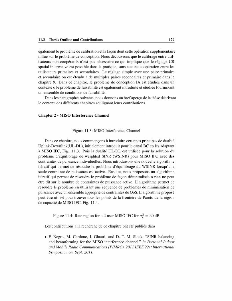
11.3 Thesis Outline and Contributions 179
egalement le probleme de calibration et la facon dont cette operation supplementaire
influe sur le probleme de conception. Nous decouvrons que le calibrage entre util-
isateurs non cooperatifs n’est pas necessaire ce qui implique que le reglage CR
spatial interweave est possible dans la pratique, sans aucune cooperation entre les
utilisateurs primaires et secondaires. Le reglage simple avec une paire primaire
et secondaire on est etendu a de multiples paires secondaires et primaire dans le
chapitre 9. Dans ce chapitre, le probleme de conception IA est etudiee dans un
contexte o le probleme de faisabilite est egalement introduite et etudiee fournissant
un ensemble de conditions de faisabilite.
Dans les paragraphes suivants, nous donnons un bref apercu de la these decrivant
le contenu des differents chapitres soulignant leurs contributions.
Chapter 2 - MISO Interference Channel
Figure 11.3: MISO Interference Channel
Dans ce chapitre, nous commencons a introduire certaines principes de dualite
Uplink-Downlink(UL-DL), initialement introduit pour le canal BC en les adaptant
a MISO IFC, Fig. 11.3. Puis la dualite UL-DL est utilisee pour la solution du
probleme d’equilibrage de weighted SINR (WSINR) pour MISO IFC avec des
contraintes de puissance individuelles. Nous introduisons une nouvelle algorithme
iteratif qui permet de resoudre le probleme d’equilibrage du WSINR lorsqu’une
seule contrainte de puissance est active. Ensuite, nous proposons un algorithme
iteratif qui permet de resoudre le probleme de facon decentralisee o rien ne peut
etre dit sur le nombre de contraintes de puissance active. L’algorithme permet de
resoudre le probleme en utilisant une sequence de problemes de minimisation de
puissance avec un ensemble approprie de contraintes de QoS. L’algorithme propose
peut etre utilise pour trouver tous les points de la frontiere de Pareto de la region
de capacite de MISO IFC, Fig. 11.4.
Figure 11.4: Rate region for a 2-user MISO IFC for σ2k = 30 dB
Les contributions a la recherche de ce chapitre ont ete publies dans
• F. Negro, M. Cardone, I. Ghauri, and D. T. M. Slock, ”SINR balancing
and beamforming for the MISO interference channel,” in Personal Indoor
and Mobile Radio Communications (PIMRC), 2011 IEEE 22st International
Symposium on, Sept. 2011.
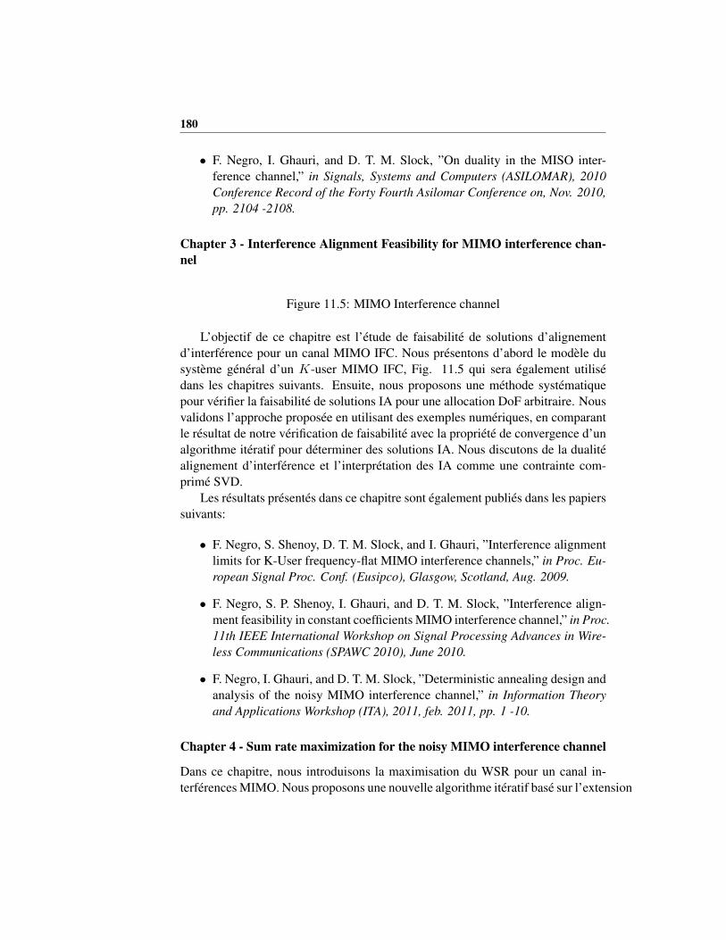
180
• F. Negro, I. Ghauri, and D. T. M. Slock, ”On duality in the MISO inter-
ference channel,” in Signals, Systems and Computers (ASILOMAR), 2010
Conference Record of the Forty Fourth Asilomar Conference on, Nov. 2010,
pp. 2104 -2108.
Chapter 3 - Interference Alignment Feasibility for MIMO interference chan-
nel
Figure 11.5: MIMO Interference channel
L’objectif de ce chapitre est l’etude de faisabilite de solutions d’alignement
d’interference pour un canal MIMO IFC. Nous presentons d’abord le modele du
systeme general d’un K-user MIMO IFC, Fig. 11.5 qui sera egalement utilise
dans les chapitres suivants. Ensuite, nous proposons une methode systematique
pour verifier la faisabilite de solutions IA pour une allocation DoF arbitraire. Nous
validons l’approche proposee en utilisant des exemples numeriques, en comparant
le resultat de notre verification de faisabilite avec la propriete de convergence d’un
algorithme iteratif pour determiner des solutions IA. Nous discutons de la dualite
alignement d’interference et l’interpretation des IA comme une contrainte com-
prime SVD.
Les resultats presentes dans ce chapitre sont egalement publies dans les papiers
suivants:
• F. Negro, S. Shenoy, D. T. M. Slock, and I. Ghauri, ”Interference alignment
limits for K-User frequency-flat MIMO interference channels,” in Proc. Eu-
ropean Signal Proc. Conf. (Eusipco), Glasgow, Scotland, Aug. 2009.
• F. Negro, S. P. Shenoy, I. Ghauri, and D. T. M. Slock, ”Interference align-
ment feasibility in constant coefficients MIMO interference channel,” in Proc.
11th IEEE International Workshop on Signal Processing Advances in Wire-
less Communications (SPAWC 2010), June 2010.
• F. Negro, I. Ghauri, and D. T. M. Slock, ”Deterministic annealing design and
analysis of the noisy MIMO interference channel,” in Information Theory
and Applications Workshop (ITA), 2011, feb. 2011, pp. 1 -10.
Chapter 4 - Sum rate maximization for the noisy MIMO interference channel
Dans ce chapitre, nous introduisons la maximisation du WSR pour un canal in-
terferences MIMO. Nous proposons une nouvelle algorithme iteratif base sur l’extension
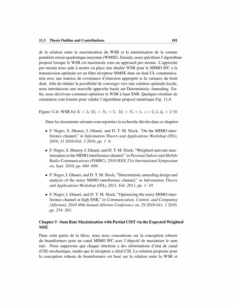
11.3 Thesis Outline and Contributions 181
de la relation entre la maximisation du WSR et la minimisation de la somme
ponderee erreur quadratique moyenne (WMSE). Ensuite, nous specifions l’algorithme
propose lorsque le WSR est maximisee sous un approach per-stream. L’approche
per-stream nous aide a mettre en place une dualite WSR pour le MIMO IFC o la
transmission optimale est un filtre recepteur MMSE dans un dual UL communica-
tion avec une matrice de covariance d’emission approprie et la variance du bruit
dual. Afin de reduire la possibilite de converger vers une solution optimale locale,
nous introduisons une nouvelle approche basee sur Deterministic Annealing. En-
fin, nous decrivons comment optimiser le WSR a haut SNR. Quelques resultats de
simulation sont fournis pour valider l’algorithme propose numerique Fig. 11.6.
Figure 11.6: WSR for K = 3, M1 = N1 = 5, Mi = Ni = 4, i = 2, 3, dk = 2 ∀k
Dans les documents suivants sont reportees la recherche decrite dans ce chapitre:
• F. Negro, S. Shenoy, I. Ghauri, and D. T. M. Slock, ”On the MIMO inter-
ference channel,” in Information Theory and Applications Workshop (ITA),
2010, 31 2010-Feb. 5 2010, pp. 1 -9.
• F. Negro, S. Shenoy, I. Ghauri, and D. T. M. Slock, ”Weighted sum rate max-
imization in the MIMO interference channel,” in Personal Indoor and Mobile
Radio Communications (PIMRC), 2010 IEEE 21st International Symposium
on, Sept. 2010, pp. 684 -689.
• F. Negro, I. Ghauri, and D. T. M. Slock, ”Deterministic annealing design and
analysis of the noisy MIMO interference channel,” in Information Theory
and Applications Workshop (ITA), 2011, Feb. 2011, pp. 1 -10.
• F. Negro, I. Ghauri, and D. T. M. Slock, ”Optimizing the noisy MIMO inter-
ference channel at high SNR,” in Communication, Control, and Computing
(Allerton), 2010 48th Annual Allerton Conference on, 29 2010-Oct. 1 2010,
pp. 254 -261.
Chapter 5 - Sum Rate Maximization with Partial CSIT via the Expected Weighted
MSE
Dans cette partie de la these, nous nous concentrons sur la conception robuste
du beamformers pour un canal MIMO IFC avec l’objectif de maximiser le sum
rate. Nous supposons que chaque emetteur a des informations d’etat de canal
(CSI) stochastique, tandis que le recepteur a ideal CSI. La solution proposee pour
la conception robuste de beamformers est base sur la relation entre la WSR et
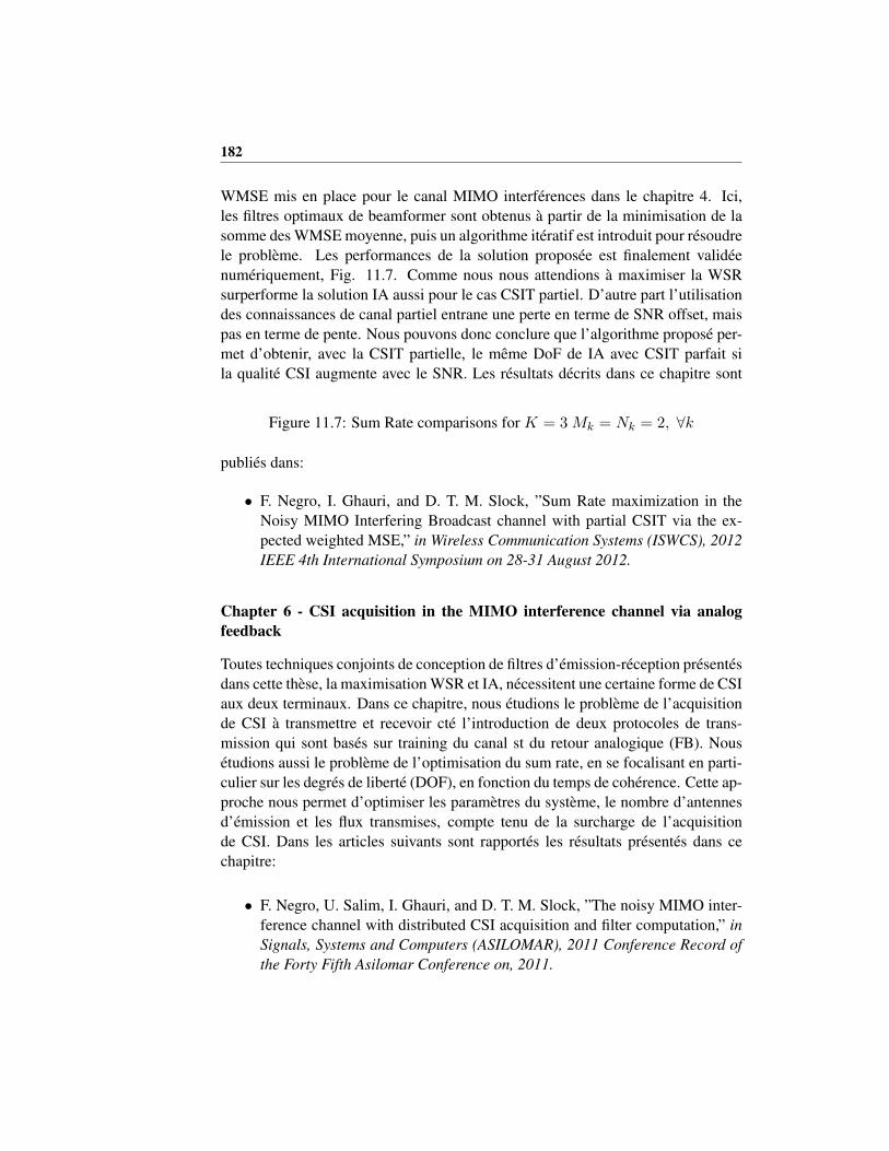
182
WMSE mis en place pour le canal MIMO interferences dans le chapitre 4. Ici,
les filtres optimaux de beamformer sont obtenus a partir de la minimisation de la
somme des WMSE moyenne, puis un algorithme iteratif est introduit pour resoudre
le probleme. Les performances de la solution proposee est finalement validee
numeriquement, Fig. 11.7. Comme nous nous attendions a maximiser la WSR
surperforme la solution IA aussi pour le cas CSIT partiel. D’autre part l’utilisation
des connaissances de canal partiel entrane une perte en terme de SNR offset, mais
pas en terme de pente. Nous pouvons donc conclure que l’algorithme propose per-
met d’obtenir, avec la CSIT partielle, le meme DoF de IA avec CSIT parfait si
la qualite CSI augmente avec le SNR. Les resultats decrits dans ce chapitre sont
Figure 11.7: Sum Rate comparisons for K = 3Mk = Nk = 2, ∀k
publies dans:
• F. Negro, I. Ghauri, and D. T. M. Slock, ”Sum Rate maximization in the
Noisy MIMO Interfering Broadcast channel with partial CSIT via the ex-
pected weighted MSE,” in Wireless Communication Systems (ISWCS), 2012
IEEE 4th International Symposium on 28-31 August 2012.
Chapter 6 - CSI acquisition in the MIMO interference channel via analog
feedback
Toutes techniques conjoints de conception de filtres d’emission-reception presentes
dans cette these, la maximisation WSR et IA, necessitent une certaine forme de CSI
aux deux terminaux. Dans ce chapitre, nous etudions le probleme de l’acquisition
de CSI a transmettre et recevoir cte l’introduction de deux protocoles de trans-
mission qui sont bases sur training du canal st du retour analogique (FB). Nous
etudions aussi le probleme de l’optimisation du sum rate, en se focalisant en parti-
culier sur les degres de liberte (DOF), en fonction du temps de coherence. Cette ap-
proche nous permet d’optimiser les parametres du systeme, le nombre d’antennes
d’emission et les flux transmises, compte tenu de la surcharge de l’acquisition
de CSI. Dans les articles suivants sont rapportes les resultats presentes dans ce
chapitre:
• F. Negro, U. Salim, I. Ghauri, and D. T. M. Slock, ”The noisy MIMO inter-
ference channel with distributed CSI acquisition and filter computation,” in
Signals, Systems and Computers (ASILOMAR), 2011 Conference Record of
the Forty Fifth Asilomar Conference on, 2011.

11.3 Thesis Outline and Contributions 183
• F. Negro, D. T. M. Slock, I. Ghauri, ”On the noisy MIMO interference chan-
nel with CSI through analog feedback,” in Communications Control and Sig-
nal Processing (ISCCSP), 2012 5th International Symposium on (ISCCSP),
2012 , pp. 1 - 6
Chapter 7 - Beamforming for the Underlay Cognitive MISO Interference Chan-
nel
Figure 11.8: Cognitive Radio DL system
Ici, nous nous concentrons sur le probleme de la conception d’un beamformer
pour reseau CR modelisee comme une canal d’interference MISO, Fig. 11.8.
Comme nous supposons de travailler dans un cadre uderlay nous avons encore
imposer un ensemble de contraintes de puissance d’interference au niveau des
recepteurs primaires. D’etendre les resultats sur UL-DL dualite a la radio cog-
nitive nous concevons le beamformers sur les emetteurs secondaires afin de min-
imiser la puissance totale emise. Nous proposons un algorithme iteratif qui per-
met de resoudre efficacement le probleme de minimisation de puissance, sur le
reseau secondaire, tout un ensemble de contraintes d’interference sont imposees
sur les recepteurs primaires. Les contributions a la recherche dans ce chapitre sont
presentes egalement dans le document suivant:
• F. Negro, I. Ghauri, and D. T. M. Slock, ”Beamforming for the underlay cog-
nitive MISO interference channel via UL-DL duality,” in Cognitive Radio
Oriented Wireless Networks Communications (CROWNCOM), 2010 Pro-
ceedings of the Fifth International Conference on, june 2010, pp. 1 -5.
Chapter 8 - Spatial Interweave TDD Cognitive Radio Systems
Figure 11.9: Downlink Channel
Dans ce chapitre, nous etudions l’optimisation conjointe des filtres d’emission-
reception dans un canal spatial interweave cognitive radio, nous decrivons toutes
les phases de communication necessaires pour acquerir les informations necessaires
aux utilisateurs primaires et secondaire. Nous mettons l’accent en particulier sur la
facon d’exploiter reellement reciprocite du canal de transmission en TDD a l’aide
UL DL calibrage etudiant comment calibrage influe emission et la conception du
filtre du recepteur sur les peripheriques primaires et secondaires. Un resultat im-
portant qui ressort de notre analyse est que la calibration non cooperatif entre Tx et

184
Rx ne sont pas necessaires pour la conception de beamformers secondaire. Nous
introduisons une extension des resultats au cas par plusieurs paires de emetteurs
et recepteurs principal. Si la conception des beamformers de reseaux primaire
selon ses IA, grce a la dualite IA, la paire secondaire peut estimer aveuglement le
sous-espace recu a tous les recepteurs primaires du sous-espace du signal transmis
dans la communication UL. Problemes calibrage sont egalement etudie dans ce
contexte prouvant que la calibration entre les utilisateurs non cooperatifs n’est pas
necessaire aussi dans le scenario approfondi. Quelques resultats de simulation sont
presentes pour valider les solutions proposees Fig.11.10. Les resultats decrits dans
Figure 11.10: Rate Comparisons
ce chapitre sont partiellement publie dans:
• F. Negro, I. Ghauri, and D. T. M. Slock, ”Transmission techniques and chan-
nel estimation for spatial interweave TDD cognitive radio systems,” in Pro-
ceedings of the 43rd Asilomar conference on Signals, systems and comput-
ers, Asilomar’09, 2009, pp. 523-527.
Chapter 9 - Spatial Interweave Cognitive Radio Interference Channel with
Multiple Primaries
Figure 11.11: Cognitive Radio System
Dans cette partie du travail que nous considerons un reseau secondaire modelise
comme un K-user MIMO IFC qui veut communiquer en presence de L recepteurs
primaires multi-antennes, Fig.11.11. Les beamformers aux utilisateurs secondaires
sont concus selon IA, a l’entrelacement des contraintes supplementaires pour generer
un sous-espace d’interference, au niveau de chaque recepteur primaire, d’une di-
mension donnee. Nous etudions la faisabilite d’une solution IA dans le systeme de
radio cognitive sous enquete sur la base des resultats presentes dans le chapitre 3.
Ensuite, nous proposons un algorithme iteratif qui trouve les emetteur et recevoir
IA secondaire satisfaisant aux contraintes s’entrecroisent au niveau des recepteurs
primaires. Les contributions de ce chapitre peuvent etre trouves dans le document
suivant:
• F. Negro, I. Ghauri, and D. T. M. Slock, ”Spatial interweave for a MIMO
secondary interference channel with multiple primary users,” in 4th Interna-
tional Conference on Cognitive Radio and Advanced Spectrum Management,
(CogART 2011), October 2011.
Bibliography
[1] A. Adhikary, V. Ntranos, and G. Caire, “Cognitive femtocells: Breaking the
spatial reuse barrier of cellular systems,” in Information Theory and Appli-
cations Workshop (ITA), 2011, feb. 2011, pp. 1 –10.
[2] D. Tse and P. Viswanath, Fundamentals of wireless communication. New
York, NY, USA: Cambridge University Press, 2005.
[3] D. Lee, H. Seo, B. Clerckx, E. Hardouin, D. Mazzarese, S. Nagata, and
K. Sayana, “Coordinated multipoint transmission and reception in LTE-
advanced: deployment scenarios and operational challenges,” Communica-
tions Magazine, IEEE, vol. 50, no. 2, pp. 148 –155, february 2012.
[4] D. Gesbert, S. Hanly, H. Huang, S. Shamai Shitz, O. Simeone, and W. Yu,
“Multi-Cell MIMO cooperative networks: A new look at interference,” Se-
lected Areas in Communications, IEEE Journal on, vol. 28, no. 9, pp. 1380
–1408, december 2010.
[5] P. Bhat, S. Nagata, L. Campoy, I. Berberana, T. Derham, G. Liu, X. Shen,
P. Zong, and J. Yang, “LTE-advanced: an operator perspective,” Communi-
cations Magazine, IEEE, vol. 50, no. 2, pp. 104 –114, february 2012.
[6] A. Carleial, “Interference channels,” IEEE Trans. on Inform. Theory,
vol. 24, no. 1, pp. 60–70, Jan 1978.
[7] ——, “A case where interference does not reduce capacity (corresp.),” In-
formation Theory, IEEE Transactions on, vol. 21, no. 5, pp. 569 – 570, sep
1975.
[8] R. H. Etkin, D. N. C. Tse, and H. Wang, “Gaussian interference channel
capacity to within one bit,” IEEE Trans. on Inform. Theory, vol. 54, no. 12,
pp. 5534–5562, 2008.
185

186 Bibliography
[9] T. Han and K. Kobayashi, “A new achievable rate region for the interference
channel,” Information Theory, IEEE Transactions on, vol. 27, no. 1, pp. 49
– 60, jan 1981.
[10] P. Viswanath and D. Tse, “Sum capacity of the multiple antenna gaussian
broadcast channel,” in Information Theory, 2002. Proceedings. 2002 IEEE
International Symposium on, 2002, p. 497.
[11] S. Vishwanath and S. Jafar, “On the capacity of vector gaussian interference
channels,” in Information Theory Workshop, 2004. IEEE, oct. 2004, pp. 365
– 369.
[12] H. Dahrouj and W. Yu, “Coordinated beamforming for the multicell multi-
antenna wireless system,” Wireless Communications, IEEE Transactions on,
vol. 9, no. 5, pp. 1748 –1759, may 2010.
[13] ——, “Coordinated beamforming for the multi-cell multi-antenna wireless
system,” in Information Sciences and Systems, 2008. CISS 2008. 42nd An-
nual Conference on, march 2008, pp. 429 –434.
[14] G. Dartmann, W. Afzal, X. Gong, and G. Ascheid, “Low complexity coop-
erative downlink beamforming in multiuser multicell networks,” in Commu-
nication Technology (ICCT), 2010 12th IEEE International Conference on,
nov. 2010, pp. 717 –721.
[15] X. Gong, M. Jordan, G. Dartmann, and G. Ascheid, “Max-min beamform-
ing for multicell downlink systems using long-term channel statistics,” in
Personal, Indoor and Mobile Radio Communications, 2009 IEEE 20th In-
ternational Symposium on, sept. 2009, pp. 803 –807.
[16] J. Lindblom and E. Karipidis, “Cooperative beamforming for the MISO
interference channel,” in Wireless Conference (EW), 2010 European, april
2010, pp. 631 –638.
[17] R. Zakhour, Z. Ho, and D. Gesbert, “Distributed beamforming coordination
in multicell MIMO channels,” in Vehicular Technology Conference, 2009.
VTC Spring 2009. IEEE 69th, april 2009, pp. 1 –5.
[18] C. Shi, R. Berry, and M. Honig, “Distributed interference pricing with MISO
channels,” in Communication, Control, and Computing, 2008 46th Annual
Allerton Conference on, sept. 2008, pp. 539 –546.

Bibliography 187
[19] E. Jorswieck, E. Larsson, and D. Danev, “Complete characterization of the
Pareto boundary for the MISO interference channel,” Signal Processing,
IEEE Transactions on, vol. 56, no. 10, pp. 5292 –5296, oct. 2008.
[20] E. Karipidis and E. G. Larsson, “Efficient computation of the Pareto bound-
ary for the MISO interference channel with perfect CSI,” in Modeling and
Optimization in Mobile, Ad Hoc and Wireless Networks (WiOpt), 2010 Pro-
ceedings of the 8th International Symposium on, 31 2010-june 4 2010, pp.
573 –577.
[21] R. Zhang and S. Cui, “Cooperative interference management with MISO
beamforming,” Signal Processing, IEEE Transactions on, vol. 58, no. 10,
pp. 5450 –5458, oct. 2010.
[22] E. Bjornson, M. Bengtsson, and B. Ottersten, “Pareto characterization of
the multicell MIMO performance region with simple receivers,” Signal Pro-
cessing, IEEE Transactions on, vol. PP, no. 99, p. 1, 2012.
[23] E. T. Ar and I. E. Telatar, “Capacity of multi-antenna Gaussian channels,”
European Transactions on Telecommunications, vol. 10, pp. 585–595, 1999.
[24] L. Zheng and D. Tse, “Diversity and multiplexing: a fundamental tradeoff
in multiple-antenna channels,” Information Theory, IEEE Transactions on,
vol. 49, no. 5, pp. 1073 – 1096, may 2003.
[25] S. Jafar and M. Fakhereddin, “Degrees of freedom for the MIMO interfer-
ence channel,” Information Theory, IEEE Transactions on, vol. 53, no. 7,
pp. 2637–2642, July 2007.
[26] M. Maddah-Ali, A. Motahari, and A. Khandani, “Signaling over MIMO
multi-base systems: Combination of multi-access and broadcast schemes,”
in Information Theory, 2006 IEEE International Symposium on, july 2006,
pp. 2104 –2108.
[27] ——, “Communication over MIMO X channels: Interference alignment, de-
composition, and performance analysis,” Information Theory, IEEE Trans-
actions on, vol. 54, no. 8, pp. 3457 –3470, aug. 2008.
[28] V. Cadambe and S. Jafar, “Interference alignment and degrees of freedom of
the K-user interference channel,” IEEE Trans. on Inform. Theory, vol. 54,
no. 8, pp. 3425 –3441, Aug. 2008.

188 Bibliography
[29] T. Gou and S. A. Jafar, “Degrees of freedom of the K user M ×N MIMO interference channel,” CoRR, vol. abs/0809.0099, 2008,
http://arxiv.org/abs/0809.0099.
[30] A. Ghasemi, A. Motahari, and A. Khandani, “Interference alignment for the
K user MIMO interference channel,” in Information Theory Proceedings
(ISIT), 2010 IEEE International Symposium on, june 2010, pp. 360 –364.
[31] R. Tresch, M. Guillaud, and E. Riegler, “On the achievability of interference
alignment in the K-user constant MIMO interference channel,” CoRR, vol.
abs/0904.4343, 2009.
[32] S. Cho, H. Chae, K. Huang, D. K. Kim, V. K. N. Lau, H. Seo,
and B.-H. Kim, “Feedback-topology designs for interference align-
ment in MIMO interference channels,” CoRR, vol. abs/1105.5476, 2011,
http://arxiv.org/abs/1105.5476.
[33] K. Gomadam, V. Cadambe, and S. Jafar, “Approaching the capacity of wire-
less networks through distributed interference alignment,” in Proc. IEEE
Global Telecommunications Conf. (GLOBECOM), Dec 2008.
[34] S. Peters and R. Heath, “Interference alignment via alternating minimiza-
tion,” in Acoustics, Speech and Signal Processing, 2009. ICASSP 2009.
IEEE International Conference on, april 2009, pp. 2445 –2448.
[35] H. Yu and Y. Sung, “Least squares approach to joint beam design for inter-
ference alignment in multiuser multi-input multi-output interference chan-
nels,” Signal Processing, IEEE Transactions on, vol. 58, no. 9, pp. 4960
–4966, sept. 2010.
[36] H. Shen, B. Li, M. Tao, and X. Wang, “MSE-based transceiver designs for
the MIMO interference channel,” Wireless Communications, IEEE Transac-
tions on, vol. 9, no. 11, pp. 3480 –3489, november 2010.
[37] C. Yetis, T. Gou, S. Jafar, and A. Kayran, “On feasibility of interference
alignment in MIMO interference networks,” Signal Processing, IEEE Trans-
actions on, vol. 58, no. 9, pp. 4771 –4782, sept. 2010.
[38] G. Bresler, D. Cartwright, and D. Tse, “Settling the feasibility of interfer-
ence alignment for the MIMO interference channel: the symmetric square
case,” CoRR, vol. abs/1104.0888, 2011, http://arxiv.org/abs/1104.0888.
[39] ——, “Geometry of the 3-user MIMO interference channel,” CoRR, vol.
abs/1110.5092, 2011, http://arxiv.org/abs/1110.5092.
Bibliography 189
[40] S. Ye and R. Blum, “Optimized signaling for MIMO interference systems
with feedback,” IEEE Trans. on Signal Processing, vol. 51, no. 11, pp.
2839–2848, Nov 2003.
[41] G. Scutari, D. Palomar, and S. Barbarossa, “Competitive design of multiuser
MIMO systems based on game theory: A unified view,” IEEE J. on Select.
Areas Commun., vol. 26, no. 7, pp. 1089 –1103, September 2008.
[42] Z. Ho and D. Gesbert, “Balancing egoism and altruism on interference chan-
nel: The MIMO case,” in Communications (ICC), 2010 IEEE International
Conference on, May 2010, pp. 1 –5.
[43] T. Bogale and L. Vandendorpe, “Weighted sum rate optimization for down-
link multiuser MIMO coordinated base station systems: Centralized and
distributed algorithms,” Signal Processing, IEEE Transactions on, vol. 60,
no. 4, pp. 1876 –1889, april 2012.
[44] Q. Shi, M. Razaviyayn, Z.-Q. Luo, and C. He, “An iteratively weighted
MMSE approach to distributed sum-utility maximization for a MIMO in-
terfering broadcast channel,” Signal Processing, IEEE Transactions on,
vol. 59, no. 9, pp. 4331 –4340, sept. 2011.
[45] S. Christensen, R. Agarwal, E. de Carvalho, and J. Cioffi, “Weighted sum-
rate maximization using weighted MMSE for MIMO-BC beamforming de-
sign,” IEEE Trans. on Wireless Communications, vol. 7, no. 12, pp. 4792–
4799, December 2008.
[46] H. Bolcskei and I. Thukral, “Interference alignment with limited feedback,”
in Information Theory, 2009. ISIT 2009. IEEE International Symposium on,
28 2009-july 3 2009, pp. 1759 –1763.
[47] R. Krishnamachari and M. Varanasi, “Interference alignment under limited
feedback for MIMO interference channels,” in Information Theory Proceed-
ings (ISIT), 2010 IEEE International Symposium on, june 2010, pp. 619
–623.
[48] O. E. Ayach and R. W. Heath Jr., “Interference alignment with
analog channel state feedback,” CoRR, vol. abs/1010.2787, 2010,
http://arxiv.org/abs/1010.2787.
[49] S. Jafar, “Exploiting channel correlations - simple interference alignment
schemes with no CSIT,” in GLOBECOM 2010, 2010 IEEE Global Telecom-
munications Conference, dec. 2010, pp. 1 –5.

190 Bibliography
[50] S. Yang, M. Kobayashi, D. Gesbert, and X. Yi, “Degrees of freedom of
time correlated MISO broadcast channel with delayed CSIT,” CoRR, vol.
abs/1203.2550, 2012, http://arxiv.org/abs/1203.2550.
[51] T. Gou and S. A. Jafar, “Optimal use of current and outdated channel state
information - degrees of freedom of the MISO BC with mixed CSIT,” CoRR,
vol. abs/1203.1301, 2012, http://arxiv.org/abs/1203.1301.
[52] X. Yi, D. Gesbert, S. Yang, and M. Kobayashi, “The DoF region of the
multiple-antenna time correlated interference channel with delayed CSIT,”
CoRR, vol. abs/1204.3046, 2012, http://arxiv.org/abs/1204.3046.
[53] FCC Spectrum Policy Task Force, “FCC report of the
spectrum efficiency working group,” [Online.] Available:
http://www.fcc.gov/sptf/files/SEWGFinalReport1.pdf, Tech. Rep., Nov.
2002.
[54] J. Mitola, “Cognitive radio: An integrated agent architecture for software de-
fined radio,” Ph.D. dissertation, Royal Inst. Tech. (KTH), Stockholm, 2000.
[55] S. Haykin, “Cognitive radio: brain-empowered wireless communications,”
Selected Areas in Communications, IEEE Journal on, vol. 23, no. 2, pp.
201–220, Feb. 2005.
[56] T. Yucek and H. Arslan, “A survey of spectrum sensing algorithms for cogni-
tive radio applications,” Communications Surveys Tutorials, IEEE, vol. 11,
no. 1, pp. 116 –130, quarter 2009.
[57] M. Mueck, A. Piipponen, K. Kallioja andrvi, G. Dimitrakopoulos,
K. Tsagkaris, P. Demestichas, F. Casadevall, J. Pe? andrez Romero, O. Sal-
lent, G. Baldini, S. Filin, H. Harada, M. Debbah, T. Haustein, J. Gebert,
B. Deschamps, P. Bender, M. Street, S. Kandeepan, J. Lota, and A. Hayar,
“ETSI reconfigurable radio systems: status and future directions on software
defined radio and cognitive radio standards,” Communications Magazine,
IEEE, vol. 48, no. 9, pp. 78 –86, sept. 2010.
[58] A. Goldsmith, S. A. Jafar, I. Maric, and S. Srinivasa, “Breaking spectrum
gridlock with cognitive radios: An information theoretic perspective,” Pro-
ceedings of the IEEE, vol. 97, no. 5, pp. 894–914, May 2009.
[59] I. Maric, A. Goldsmith, G. Kramer, and S. Shamai, “On the capacity of
interference channels with a cognitive transmitter,” in Information Theory
and Applications Workshop, 2007, feb 2007, pp. 268–273.
Bibliography 191
[60] W. Wu, S. Vishwanath, and A. Arapostathis, “Capacity of a class of cog-
nitive radio channels: Interference channels with degraded message sets,”
Information Theory, IEEE Transactions on, vol. 53, no. 11, pp. 4391 –4399,
nov. 2007.
[61] I. Maric, A. Goldsmith, G. Kramer, and S. Shamai, “On the capacity of inter-
ference channels with one cooperating transmitter,” European Transactions
on Telecommunications, vol. 19, pp. 405–420, Apr. 2008.
[62] M. Gastpar, “On capacity under receive and spatial spectrum-sharing con-
straints,” Information Theory, IEEE Transactions on, vol. 53, no. 2, pp. 471
–487, feb. 2007.
[63] A. Ghasemi and E. Sousa, “Capacity of fading channels under spectrum-
sharing constraints,” in Communications, 2006. ICC ’06. IEEE International
Conference on, vol. 10, june 2006, pp. 4373 –4378.
[64] R. Zhang and Y.-C. Liang, “Exploiting multi-antennas for opportunistic
spectrum sharing in cognitive radio networks,” Selected Topics in Signal
Processing, IEEE Journal of, vol. 2, no. 1, pp. 88 –102, feb. 2008.
[65] L. Zhang, Y.-C. Liang, and Y. Xin, “Joint beamforming and power allocation
for multiple access channels in cognitive radio networks,” Selected Areas in
Communications, IEEE Journal on, vol. 26, no. 1, pp. 38 –51, jan. 2008.
[66] M. Pesavento, D. Ciochina, and A. Gershman, “Iterative dual downlink
beamforming for cognitive radio networks,” in Cognitive Radio Oriented
Wireless Networks Communications (CROWNCOM), 2010 Proceedings of
the Fifth International Conference on, june 2010, pp. 1 –5.
[67] I. Wajid, H. Nikolaeva, and M. Pesavento, “Iterative robust downlink beam-
forming in cognitive radio networks,” in Cognitive Radio Oriented Wireless
Networks and Communications (CROWNCOM), 2011 Sixth International
ICST Conference on, june 2011, pp. 375 –379.
[68] F. Wang and W. Wang, “Sum rate optimization in interference channel of
cognitive radio network,” in Communications (ICC), 2010 IEEE Interna-
tional Conference on, may 2010, pp. 1 –5.
[69] S.-J. Kim and G. Giannakis, “Optimal resource allocation for MIMO ad
hoc cognitive radio networks,” Information Theory, IEEE Transactions on,
vol. 57, no. 5, pp. 3117 –3131, may 2011.

192 Bibliography
[70] G. Scutari, D. Palomar, and S. Barbarossa, “Cognitive MIMO radio,” Signal
Processing Magazine, IEEE, vol. 25, no. 6, pp. 46 –59, november 2008.
[71] B. Wang, Y. Wu, and K. J. R. Liu, “Game theory for cognitive radio net-
works: An overview,” Computer Networks, vol. 54, no. 14, pp. 2537–2561,
2010.
[72] F. Gao, R. Zhang, Y.-C. Liang, and X. Wang, “Design of learning-based
MIMO cognitive radio systems,” Vehicular Technology, IEEE Transactions
on, vol. 59, no. 4, pp. 1707 –1720, may 2010.
[73] R. Zhang, F. Gao, and Y.-C. Liang, “Cognitive beamforming made practical:
Effective interference channel and learning-throughput tradeoff,” Communi-
cations, IEEE Transactions on, vol. 58, no. 2, pp. 706 –718, february 2010.
[74] L. Cardoso, M. Kobayashi, O. Ryan, and M. Debbah, “Vandermonde fre-
quency division multiplexing for cognitive radio,” in Signal Processing Ad-
vances in Wireless Communications, 2008. SPAWC 2008. IEEE 9th Work-
shop on, july 2008, pp. 421 –425.
[75] H. Boche and M. Schubert, “A general duality theory for uplink and down-
link beamforming,” vol. 1, 2002, pp. 87 – 91 vol.1.
[76] M. Schubert and H. Boche, “Solution of the multiuser downlink beamform-
ing problem with individual SINR constraints,” Vehicular Technology, IEEE
Transactions on, vol. 53, no. 1, pp. 18 – 28, jan. 2004.
[77] P. Viswanath and D. Tse, “Sum capacity of the vector gaussian broadcast
channel and uplink-downlink duality,” Information Theory, IEEE Transac-
tions on, vol. 49, no. 8, pp. 1912 – 1921, aug. 2003.
[78] M. Costa, “Writing on dirty paper (corresp.),” Information Theory, IEEE
Transactions on, vol. 29, no. 3, pp. 439 – 441, may 1983.
[79] J. Yang and D. K. Kim, “Multi-cell uplink-downlink beamforming through-
put duality based on lagrangian duality with per-base station power con-
straints,” Communications Letters, IEEE, vol. 12, no. 4, pp. 277 –279, april
2008.
[80] G. Montalbano, I. Ghauri, and D. Slock, “Spatio-temporal array processing
for CDMA/SDMA downlink transmission,” in Signals, Systems amp; Com-
puters, 1998. Conference Record of the Thirty-Second Asilomar Conference
on, vol. 2, nov. 1998, pp. 1337 –1341 vol.2.

Bibliography 193
[81] H. Boche and M. Schubert, “SIR balancing for multiuser downlink beam-
forming - a convergence analysis,” in Communications, 2002. ICC 2002.
IEEE International Conference on, vol. 2, 2002, pp. 841 – 845 vol.2.
[82] M. Schubert, N. Vucic, and H. Boche, “SIR balancing for strongly con-
nected interference networks - existence and uniqueness of a solution,” in
Wireless Communication Systems (ISWCS), 2010 7th International Sympo-
sium on, sept. 2010, pp. 184 –188.
[83] D. Cai, T. Quek, and C. W. Tan, “Max-min weighted SIR for MIMO down-
link system: Optimality and algorithms,” in Information Theory Proceed-
ings (ISIT), 2010 IEEE International Symposium on, june 2010, pp. 2118
–2122.
[84] D. W. H. Cai, T. Queck, and C. W. Tan, “Coordinated max-min SIR opti-
mization in multicell downlink - duality and algorithm,” in Communications
(ICC), 2010 IEEE International Conference on, June 2011.
[85] E. Larsson and E. Jorswieck, “Competition versus cooperation on the MISO
interference channel,” Selected Areas in Communications, IEEE Journal on,
vol. 26, no. 7, pp. 1059 –1069, september 2008.
[86] R. Mochaourab and E. Jorswieck, “Optimal beamforming in interference
networks with perfect local channel information,” Signal Processing, IEEE
Transactions on, vol. 59, no. 3, pp. 1128 –1141, march 2011.
[87] ——, “Exchange economy in two-user multiple-input single-output inter-
ference channels,” Selected Topics in Signal Processing, IEEE Journal of,
vol. 6, no. 2, pp. 151 –164, april 2012.
[88] P. Cao, S. Shi, and E. Jorswieck, “Efficient Computation of the Pareto
Boundary for the Two-User MIMO Interference Channel,” in submitted to
SPAWC, 2012.
[89] H. Mahdavi-Doost, M. Ebrahimi, and A. Khandani, “Characterization of
SINR region for interfering links with constrained power,” Information The-
ory, IEEE Transactions on, vol. 56, no. 6, pp. 2816 –2828, june 2010.
[90] W. Yu and T. Lan, “Transmitter optimization for the multi-antenna down-
link with per-antenna power constraints,” IEEE Trans. on Signal Processing,
vol. 55, no. 6, June 2007.

194 Bibliography
[91] A. Wiesel, Y. Eldar, and S. Shamai, “Linear precoding via conic optimiza-
tion for fixed MIMO receivers,” Signal Processing, IEEE Transactions on,
vol. 54, no. 1, pp. 161 – 176, jan. 2006.
[92] S. Boyd and L. Vandenberghe, Convex Optimization. Cambridge U.K.:
Cambridge Univ. Press,, 2004.
[93] G. Montalbano and D. Slock, “Matched filter bound optimization for mul-
tiuser downlink transmit beamforming,” in Universal Personal Communi-
cations, 1998. ICUPC ’98. IEEE 1998 International Conference on, vol. 1,
Oct. 1998, pp. 677 –681 vol.1.
[94] W. Yang and G. Xu, “Optimal downlink power assignment for smart antenna
systems,” in Acoustics, Speech and Signal Processing, 1998. Proceedings of
the 1998 IEEE International Conference on, vol. 6, May 1998, pp. 3337
–3340 vol.6.
[95] V. Blondel, L. Ninove, and P. Vandooren, “An affine eigenvalue problem on
the nonnegative orthant,” Linear Algebra and Its Applications, vol. 404, pp.
69–84, 2005.
[96] G. Bresler, A. Parekh, and D. Tse, “The approximate capacity of the many-
to-one and one-to-many gaussian interference channels,” Information The-
ory, IEEE Transactions on, vol. 56, no. 9, pp. 4566 –4592, sept. 2010.
[97] V. R. Cadambe, S. A. Jafar, and S. Shamai, “Interference align-
ment on the deterministic channel and application to fully con-
nected AWGN interference networks,” CoRR, vol. abs/0711.2547, 2007,
http://arxiv.org/abs/0711.2547.
[98] A. S. Motahari, S. O. Gharan, M. A. Maddah-Ali, and A. K. Khandani,
“Forming pseudo-MIMO by embedding infinite rational dimensions along
a single real line: Removing barriers in achieving the dofs of single antenna
systems,” CoRR, vol. abs/0908.2282, 2009, http://arxiv.org/abs/0908.2282.
[99] B. Zhuang, R. A. Berry, and M. L. Honig, “Interference alignment in MIMO
cellular networks,” in Acoustics, Speech and Signal Processing (ICASSP),
2011 IEEE International Conference on, may 2011, pp. 3356 –3359.
[100] Y.-F. Liu, Y.-H. Dai, and Z.-Q. Luo, “On the complexity of leakage in-
terference minimization for interference alignment,” in Signal Processing
Advances in Wireless Communications (SPAWC), 2011 IEEE 12th Interna-
tional Workshop on, june 2011, pp. 471 –475.

Bibliography 195
[101] O. Gonzalez, C. Beltran, and I. Santamarıa, “On the feasibility of interfer-
ence alignment for the k-user MIMO channel with constant coefficients,”
CoRR, vol. abs/1202.0186, 2012, http://arxiv.org/abs/1202.0186.
[102] N. Lee, D. Park, and Y.-D. Kim, “Degrees of freedom on the K-user MIMO
interference channel with constant channel coefficients for downlink com-
munications,” in Global Telecommunications Conference, 2009. GLOBE-
COM 2009. IEEE, 30 2009-dec. 4 2009, pp. 1 –6.
[103] M. Westreicher and M. Guillaud, “Interference alignment over partially con-
nected interference networks: Application to the cellular case,” IEEE Wire-
less Communications and Networking Conference (WCNC), Paris, France,
Apr. 1-4, 2012.
[104] M. Guillaud and D. Gesbert, “Interference alignment in the partially con-
nected K-user MIMO interference channel,” European Signal Processing
Conference (EUSIPCO), Barcelona, Spain (invited); Aug. 29-Sep. 2, 2011.
[105] ——, “Interference alignment in partially connected interfering multiple-
access and broadcast channels,” IEEE Global Telecommunications Confer-
ence (GLOBECOM), Houston, TX, USA, Dec. 5-9, 2011.
[106] F. Negro, S. P. Shenoy, D. T. M. Slock, and I. Ghauri, “Interference align-
ment limits for K-user frequency-flat MIMO,” in Eusipco 2009, 17th Eu-
ropean Signal Processing Conference, August 24-28, 2009, Glasgow, Scot-
land, Glasgow, UK, 08 2009.
[107] E. Allgower and K. Georg, “Introduction to numerical continuation meth-
ods,” Philadelphia, PA: Society for Industrial and Applied Mathematics,
2003.
[108] O. Gonzalez and I. Santamaria, “Interference alignment in single-beam
MIMO networks via homotopy continuation,” in Acoustics, Speech and Sig-
nal Processing (ICASSP), 2011 IEEE International Conference on, may
2011, pp. 3344 –3347.
[109] J. Yang and S. Roy, “On joint transmitter and receiver optimization for
multiple-input-multiple-output (MIMO) transmission systems,” Communi-
cations, IEEE Transactions on, vol. 42, no. 12, pp. 3221 –3231, dec 1994.
[110] H. Sampath, P. Stoica, and A. Paulraj, “Generalized linear precoder and
decoder design for MIMO channels using the weighted MMSE criterion,”
Communications, IEEE Transactions on, vol. 49, no. 12, pp. 2198 –2206,
dec 2001.
196 Bibliography
[111] D. Palomar, J. Cioffi, and M. Lagunas, “Joint Tx-Rx beamforming design for
multicarrier MIMO channels: a unified framework for convex optimization,”
Signal Processing, IEEE Transactions on, vol. 51, no. 9, pp. 2381 – 2401,
sept. 2003.
[112] L.-U. Choi and R. Murch, “A transmit preprocessing technique for mul-
tiuser MIMO systems using a decomposition approach,” Wireless Commu-
nications, IEEE Transactions on, vol. 3, no. 1, pp. 20 – 24, jan. 2004.
[113] S. Serbetli and A. Yener, “Transceiver optimization for multiuser MIMO
systems,” Signal Processing, IEEE Transactions on, vol. 52, no. 1, pp. 214
– 226, jan. 2004.
[114] M. Stojnic, H. Vikalo, and B. Hassibi, “Rate maximization in multi-antenna
broadcast channels with linear preprocessing,” IEEE Trans. on Wireless
Communications, vol. 5, no. 9, pp. 2338 –2342, September 2006.
[115] S. Shi, M. Schubert, and H. Boche, “Rate optimization for multiuser MIMO
systems with linear processing,” Signal Processing, IEEE Transactions on,
vol. 56, no. 8, pp. 4020 –4030, aug. 2008.
[116] S. Shi and M. Schubert, “MMSE transmit optimization for multi-user multi-
antenna systems,” in Acoustics, Speech, and Signal Processing, 2005. Pro-
ceedings. (ICASSP ’05). IEEE International Conference on, vol. 3, march
2005, pp. iii/409 – iii/412 Vol. 3.
[117] S. Shi, M. Schubert, and H. Boche, “Downlink MMSE transceiver optimiza-
tion for multiuser MIMO systems: Duality and Sum-MSE minimization,”
Signal Processing, IEEE Transactions on, vol. 55, no. 11, pp. 5436 –5446,
nov. 2007.
[118] H. Sung, S.-H. Park, K.-J. Lee, and I. Lee, “Linear precoder designs for K-
user interference channels,” Wireless Communications, IEEE Transactions
on, vol. 9, no. 1, pp. 291 –301, jan. 2010.
[119] D. Schmidt, C. Shi, R. Berry, M. Honig, and W. Utschick, “Distributed
resource allocation schemes,” Signal Processing Magazine, IEEE, vol. 26,
no. 5, pp. 53 –63, september 2009.
[120] M. Joham, K. Kusume, M. Gzara, W. Utschick, and J. Nossek, “Transmit
Wiener filter for the downlink of TDDDS-CDMA systems,” in Spread Spec-
trum Techniques and Applications, 2002 IEEE Seventh International Sym-
posium on, vol. 1, 2002, pp. 9 – 13 vol.1.
Bibliography 197
[121] D. A. Schmidt, W. Utschick, and M. L. Honig, “Beamforming techniques
for single-beam MIMO interference networks,” in Communication, Control,
and Computing (Allerton), 2010 48th Annual Allerton Conference on, 29
2010-oct. 1 2010, pp. 1182 –1187.
[122] S. Gesualdo, D. P. Palomar, and S. Barbarossa, “The MIMO iterative wa-
terfilling algorithm,” IEEE Trans. on Signal Processing, vol. 57, no. 5, pp.
1917–1935, May 2009.
[123] S. Changxin, D. A. Schmidt, R. A. Berry, M. L. Honig, and W. Utschick,
“Distributed interference pricing for the MIMO interference channel,” in
Proc. IEEE Int’l Communications Conf. (ICC), Dresden, Germany, 2009.
[124] F. Negro, S. Shenoy, I. Ghauri, and D. Slock, “On the MIMO interference
channel,” in Information Theory and Applications Workshop (ITA), 2010, 31
2010-feb. 5 2010, pp. 1 –9.
[125] M. Joham, K. Kusume, M. Gzara, W. Utschick, and J. Nossek, “Transmit
Wiener Filter,” Munich University of Technology, Tech. Rep., January 2002.
[126] K. B. Petersen and M. S. Pedersen, “The matrix cookbook,” oct 2008, ver-
sion 20081110, http://www2.imm.dtu.dk/pubdb/p.php?3274.
[127] F. Negro, S. Shenoy, D. Slock, and I. Ghauri, “Interference Alignment Lim-
its for K-User Frequency-Flat MIMO Interference Channels,” in Proc. Eu-
ropean Signal Proc. Conf. (Eusipco), Glasgow, Scotland, Aug. 2009.
[128] K. Rose, “Deterministic annealing for clustering, compression, classifica-
tion, regression, and related optimization problems,” Proceedings of the
IEEE, vol. 86, no. 11, pp. 2210 –2239, nov 1998.
[129] F. Negro, I. Ghauri, and D. T. Slock, “Optimizing the noisy MIMO inter-
ference channel at high SNR,” in Communication, Control, and Computing
(Allerton), 2010 48th Annual Allerton Conference on, 29 2010-oct. 1 2010,
pp. 254 –261.
[130] C. Hellings, D. A. Schmidt, and W. Utschick, “Optimized beamforming for
the two stream MIMO interference channel at high SNR,” in Proc. Interna-
tional ITG Workshop on Smart Antennas - WSA 2009, February 2009.
[131] J. Wang and D. Palomar, “Robust MMSE precoding in MIMO channels
with pre-fixed receivers,” Signal Processing, IEEE Transactions on, vol. 58,
no. 11, pp. 5802 –5818, nov. 2010.
198 Bibliography
[132] E. A. Jorswieck, A. Sezgin, H. Boche, and E. Costa, “Multiuser MIMO
MAC with statistical CSI and MMSE receiver: feedback strategies
and transmitter optimization,” in Proceedings of the 2006 international
conference on Wireless communications and mobile computing, ser.
IWCMC ’06. New York, NY, USA: ACM, 2006, pp. 455–460. [Online].
Available: http://doi.acm.org/10.1145/1143549.1143640
[133] N. Vucic, H. Boche, and S. Shi, “Robust transceiver optimization in down-
link multiuser mimo systems,” Signal Processing, IEEE Transactions on,
vol. 57, no. 9, pp. 3576 –3587, sept. 2009.
[134] A. Tajer, N. Prasad, and X. Wang, “Robust transceiver design for the multi-
user interference channel,” in Communications (ICC), 2010 IEEE Interna-
tional Conference on, may 2010, pp. 1 –5.
[135] R. Mochaourab and E. Jorswieck, “Robust Beamforming in Interference
Channels with Imperfect Transmitter Channel Information,” Signal
Processing, vol. 92, no. 10, pp. 2509–2518, 2012. [Online]. Available:
http://dx.doi.org/10.1016/j.sigpro.2012.03.014
[136] H. Shen, B. Li, M. Tao, and X. Wang, “Mse-based transceiver designs for the
mimo interference channel,” Wireless Communications, IEEE Transactions
on, vol. 9, no. 11, pp. 3480 –3489, november 2010.
[137] E. Chiu, V. Lau, T. Wu, S. Liu, and Y. Cui, “Robust transceiver design for K-
pairs quasi-static MIMO interference channels via semi-definite relaxation,”
in Signals, Systems and Computers (ASILOMAR), 2010 Conference Record
of the Forty Fourth Asilomar Conference on, nov. 2010, pp. 2094 –2098.
[138] J. Jose, N. Prasad, M. Khojastepour, and S. Rangarajan, “On robust
weighted-sum rate maximization in MIMO interference networks,” in Com-
munications (ICC), 2011 IEEE International Conference on, june 2011, pp.
1 –6.
[139] H. Park, S.-H. Park, H.-B. Kong, and I. Lee, “Weighted sum MSE minimiza-
tion under per-BS power constraint for network MIMO systems,” Commu-
nications Letters, IEEE, vol. 16, no. 3, pp. 360 –363, march 2012.
[140] U. Salim and D. T. M. Slock, “How much feedback is required for TDD
multi-antenna broadcast channels with user selection ?” EURASIP Journal
on Advances in Signal Processing; Vol. 2010 (2010), Article ID 278952, 05
2010. [Online]. Available: http://www.eurecom.fr/publication/3175
Bibliography 199
[141] B. Hassibi and B. Hochwald, “How much training is needed in multiple-
antenna wireless links?” Information Theory, IEEE Transactions on, vol. 49,
no. 4, pp. 951 – 963, april 2003.
[142] L. Zheng and D. Tse, “Communication on the Grassmann manifold: a geo-
metric approach to the noncoherent multiple-antenna channel,” Information
Theory, IEEE Transactions on, vol. 48, no. 2, pp. 359 –383, feb 2002.
[143] A. Dana, M. Sharif, and B. Hassibi, “On the capacity region of multi-
antenna gaussian broadcast channels with estimation error,” in Information
Theory, 2006 IEEE International Symposium on, july 2006, pp. 1851 –1855.
[144] M. Kobayashi, G. Caire, and N. Jindal, “How much training and feedback
are needed in MIMO broadcast channels?” in Information Theory, 2008.
ISIT 2008. IEEE International Symposium on, july 2008, pp. 2663 –2667.
[145] M. Kobayashi, N. Jindal, and G. Caire, “Training and feedback optimization
for multiuser MIMO downlink,” Communications, IEEE Transactions on,
vol. 59, no. 8, pp. 2228 –2240, august 2011.
[146] G. Kramer, “Feedback strategies for white gaussian interference networks,”
Information Theory, IEEE Transactions on, vol. 48, no. 6, pp. 1423 –1438,
jun 2002.
[147] M. Gastpar and G. Kramer, “On noisy feedback for interference channels,”
in Signals, Systems and Computers, 2006. ACSSC ’06. Fortieth Asilomar
Conference on, 29 2006-nov. 1 2006, pp. 216 –220.
[148] C. Suh and D. Tse, “Feedback capacity of the gaussian interference channel
to within 2 bits,” Information Theory, IEEE Transactions on, vol. 57, no. 5,
pp. 2667 –2685, may 2011.
[149] D. Tuninetti, “On interference channel with generalized feedback (IFC-
GF),” in Information Theory, 2007. ISIT 2007. IEEE International Sympo-
sium on, june 2007, pp. 2861 –2865.
[150] S. Cho, H. Chae, K. Huang, D. K. Kim, V. K. N. Lau, H. Seo,
and B.-H. Kim, “Feedback-topology designs for interference align-
ment in mimo interference channels,” CoRR, vol. abs/1105.5476, 2011,
http://arxiv.org/abs/1105.5476.
[151] M. A. Maddah-Ali and D. Tse, “Completely stale transmitter channel
state information is still very useful,” CoRR, vol. abs/1010.1499, 2010,
http://arxiv.org/abs/1010.1499.
200 Bibliography
[152] C. Vaze and M. Varanasi, “The degrees of freedom region of the MIMO in-
terference channel with delayed CSIT,” in Information Theory Proceedings
(ISIT), 2011 IEEE International Symposium on, 31 2011-aug. 5 2011, pp.
2203 –2207.
[153] R. Tandon, S. Mohajer, H. V. Poor, and S. Shamai, “On interference net-
works with feedback and delayed CSI,” CoRR, vol. abs/1109.5373, 2011,
http://arxiv.org/abs/1109.5373.
[154] C. S. Vaze and M. K. Varanasi, “The degrees of freedom region of
the MIMO interference channel with Shannon feedback,” CoRR, vol.
abs/1109.5779, 2011, http://arxiv.org/abs/1109.5779.
[155] F. Negro, U. Salim, I. Ghauri, and D. Slock, “The noisy MIMO interference
channel with distributed CSI acquisition and filter computation,” in Proc.
Asilomar Conf. on Signals, Systems, and Computers, Pacific Grove, CA,
USA, Nov. 2011.
[156] K. Hamdi, W. Zhang, and K. Ben Letaief, “Joint beamforming and schedul-
ing in cognitive radio networks,” in Global Telecommunications Conference,
2007. GLOBECOM ’07. IEEE, nov. 2007, pp. 2977 –2981.
[157] G. Zheng, S. Ma, K.-K. Wong, and T.-S. Ng, “Robust beamforming in cog-
nitive radio,” in Vehicular Technology Conference, 2009. VTC Spring 2009.
IEEE 69th, april 2009, pp. 1 –4.
[158] K. Cumanan, R. Krishna, V. Sharma, and S. Lambotharan, “Robust inter-
ference control techniques for multiuser cognitive radios using worst-case
performance optimization,” in Signals, Systems and Computers, 2008 42nd
Asilomar Conference on, oct. 2008, pp. 378 –382.
[159] M. Pesavento, D. Ciochina, and A. Gershman, “Iterative dual downlink
beamforming for cognitive radio networks,,” submitted to CROWNCOM
2010, June 2010.
[160] K. Cumanan, L. Musavian, S. Lambotharan, and A. Gershman, “SINR bal-
ancing technique for downlink beamforming in cognitive radio networks,”
Signal Processing Letters, IEEE, vol. 17, no. 2, pp. 133 –136, feb. 2010.
[161] K. Cumanan, R. Krishna, Z. Xiong, and S. Lambotharan, “SINR balanc-
ing technique and its comparison to semidefinite programming based QoS
provision for cognitive radios,” in Vehicular Technology Conference, 2009.
VTC Spring 2009. IEEE 69th, april 2009, pp. 1 –5.

Bibliography 201
[162] M. Hanif, P. Smith, and M. Alouini, “SINR balancing in the downlink of
cognitive radio networks with imperfect channel knowledge,” in Cognitive
Radio Oriented Wireless Networks Communications (CROWNCOM), 2010
Proceedings of the Fifth International Conference on, june 2010, pp. 1 –5.
[163] A. Tajer, N. Prasad, and X. Wang, “Beamforming and rate allocation in
miso cognitive radio networks,” Signal Processing, IEEE Transactions on,
vol. 58, no. 1, pp. 362 –377, jan. 2010.
[164] H. Du, T. Ratnarajah, M. Pesavento, and C. Papadias, “Joint transceiver
beamforming in MIMO cognitive radio network via second-order cone pro-
gramming,” Signal Processing, IEEE Transactions on, vol. 60, no. 2, pp.
781 –792, feb. 2012.
[165] S. Boyd, “Subgradient methods,”
http://www.stanford.edu/class/ee392o/subgrad method.pdf.
[166] N. Jamal and P. Mitran, “Performance analysis of null-steering beamform-
ers in cognitive radio systems,” in Global Telecommunications Conference
(GLOBECOM 2011), 2011 IEEE, dec. 2011, pp. 1 –6.
[167] Z. Xiong, R. Krishna, K. Cumanan, and S. Lambotharan, “Grassmannian
beamforming and null space broadcasting protocols for cognitive radio net-
works,” Signal Processing, IET, vol. 5, no. 5, pp. 451 –460, august 2011.
[168] E. Jorswieck and R. Mochaourab, “Beamforming in underlay cognitive ra-
dio: Null-shaping constraints and greedy user selection,” in Cognitive Radio
Oriented Wireless Networks Communications (CROWNCOM), 2010 Pro-
ceedings of the Fifth International Conference on, june 2010, pp. 1 –5.
[169] S. Perlaza, M. Debbah, S. Lasaulce, and J.-M. Chaufray, “Opportunistic
interference alignment in MIMO interference channels,” in Personal, Indoor
and Mobile Radio Communications. PIMRC 2008. IEEE 19th International
Symposium on, Sept. 2008, pp. 1–5.
[170] F. Negro, I. Ghauri, and D. Slock, “Transmission techniques and channel
estimation for spatial interweave TDD cognitive radio systems,” in Signals,
Systems and Computers, 2009 Conference Record of the 43rd Asilomar Con-
ference on, nov. 2009, pp. 523–527.
[171] M. Guillaud, D. T. M. Slock, and R. Knopp, “A practical method for wire-
less channel reciprocity exploitation through relative calibration,” in ISSPA
2005, 8th International Symposium on Signal Processing and Its Applica-
tions, Sydney, Australia, Aug 2005.
202 Bibliography
[172] J. Liu, G. Vandersteen, J. Craninckx, M. Libois, M. Wouters, F. Petre, and
A. Barel, “A novel and low-cost analog front-end mismatch calibration
scheme for MIMO-OFDM WLANs,” in Radio and Wireless Symposium,
2006 IEEE, pp. 219–222.
[173] B. Kouassi, I. Ghauri, B. Zayen, and L. Deneire, “On the performance of cal-
ibration techniques for cognitive radio systems,” in The 14th International
Symposium WPMC’11, Brest, France, oct 2011.
[174] W. Yu, W. Rhee, S. Boyd, and J. Cioffi, “Iterative water-filling for gaussian
vector multiple-access channels,” Information Theory, IEEE Transactions
on, vol. 50, no. 1, pp. 145–152, Jan. 2004.
[175] M. Wax and T. Kailath, “Detection of signals by information theoretic cri-
teria,” Acoustics, Speech and Signal Processing, IEEE Transactions on,
vol. 33, no. 2, pp. 387–392, apr 1985.
[176] H. Yi, “Nullspace-based secondary joint transceiver scheme for cognitive
radio MIMO networks using second-order statistics,” in Communications
(ICC), 2010 IEEE International Conference on, may 2010, pp. 1–5.
[177] F. Li, H. Liu, and R. Vaccaro, “Performance analysis for DOA estimation
algorithms: unification, simplification, and observations,” Aerospace and
Electronic Systems, IEEE Transactions on, vol. 29, no. 4, pp. 1170–1184,
oct 1993.
[178] D. Sacristan and A. Pascual-Iserte, “Differential feedback of MIMO channel
correlation matrices based on geodesic curves,” in Acoustics, Speech and
Signal Processing, 2009. ICASSP 2009. IEEE International Conference on,
April 2009, pp. 2553–2556.
[179] D. Maiwald and D. Kraus, “Calculation of moments of complex Wishart
and complex inverse Wishart distributed matrices,” Radar, Sonar and Navi-
gation, IEEE Proceedings, vol. 147, no. 4, pp. 162–168, aug 2000.
[180] C. Shen and M. Fitz, “Dynamic spatial spectrum access with opportunistic
orthogonalization,” in Information Sciences and Systems, 2009. CISS 2009.
43rd Annual Conference on, march 2009, pp. 600 –605.
[181] M. Amir, A. El-Keyi, and M. Nafie, “Opportunistic interference alignment
for multiuser cognitive radio,” in Information Theory Workshop (ITW), 2010
IEEE, jan. 2010, pp. 1 –5.
Bibliography 203
[182] H. Zhou, T. Ratnarajah, and Y.-C. Liang, “On secondary network interfer-
ence alignment in cognitive radio,” in New Frontiers in Dynamic Spectrum
Access Networks (DySPAN), 2011 IEEE Symposium on, may 2011, pp. 637
–641.
[183] B. Nosrat-Makouei, J. G. Andrews, and R. W. Heath, “User admission in
mimo interference alignment networks,” in Acoustics, Speech and Signal
Processing (ICASSP), 2011 IEEE International Conference on, may 2011,
pp. 3360 –3363.
[184] F. Negro, S. P. Shenoy, I. Ghauri, and D. Slock, “Interference Align-
ment Feasibility in Constant Coefficients MIMO Interference Channel,” in
Proc. 11th IEEE Int’l Workshop on Signal Processing Advances in Wireless
Comm’s (SPAWC), June 2010.
Related Documents