Transmission Losses Executive Summary and Tariffs/Price ang Tariffs 2008/KOST SH_A... · 4 load. It also and used values of new over head line resistance derived form manufacturers

KOSTT • Iljaz Kodra St. n.n, 10 000 Prishtina, Kosovo • Ph: +381(0) 38 501 601 5 • Fax:+381(0)38 500 201 • email: [email protected] • Web: www.kostt.com • Business Reg. No.: 70325350

04.12.2007

Transmission Losses Executive Summary

1. Executive Summary

For some time, KOSTT has been concerned that the volume (and cost to them) of the losses due

to Kosovo demand and to transits through the transmission network, have been running at

significantly higher levels than allowed for in the 2007-09 Price Control.

In association with its Consultants, KOSTT has recently carried out its own analysis of losses: of

actual metered losses between January 2006 and October 2007; and predictive studies of 2007-

09 annual losses, using both the ‘standard’ method described in the report of ESTAP I (Module

D) and an alternative method (based on PSSE – Power System Simulation for Engineers) which

is considered a better representation of the range of conditions to be expected in the system at

various levels of demand. The results of these analyses all lead to broadly the same results,

strongly suggesting that they are soundly based.

Analysis of the actual metered data shows that losses due to transits are themselves

unpredictable, and KOSTT can neither control or influence the level of transits through its

system. This is indicated in the histogram below:-

It therefore appears not appropriate for incentives to be applied to transit losses.

Histogram of TransitsApr-Sep 2007

0%

2%

4%

6%

8%

10%

12%

0

139

199

259

319

379

439

499

559

619

679

2

Both methods of analysing 2007-09 predicted losses due to Kosovo demand lead to substantially

the same result, as tabulated below:-

Standard method PSSE method

Year

Kosovan demand supplied [GWh]

Losses at Allowed TLF of

1.03 Estimated

losses [GWh] TLF(load) Estimated losses [GWh] TLF(load)

2007 4865 146.0 177.3 1.036 185.3 1.038

2008 5115 153.5 200.7 1.039 199.5 1.039

2009 5427 162.8 217.7 1.040 224.6 1.041 Total 2007-09 15407 462.2 595.7 1.039 609.4 1.041

It is KOSTT’s contention that these losses will be substantially greater that those allowed for in

the 2007-09 Price Control, and that the extra cost of paying for these losses will exceed the

revenue allowed for their purchase by some €3.7M. Furthermore, unless this discrepancy is

quickly addressed, this additional and unforeseen expenditure will impose a significant burden

on KOSTT that both threatens their financial viability as a business, and will materially affect

their ability to invest in the transmission system.

Transmission Losses - Regulatory review

Introduction

The Allowed Revenues for Transmission Losses were determined in November 2006 by the ERO1 based on Tariffs Methodology as adopted by ERO.

By November 2006, when the revenues were determined, many important data sources were not available and KOSTT used a pragmatic approach in order to determine the materiality of the both transit and Kosova transmission losses.

1 Tariff Methodology for the Electricity Sector – Including amendments to 15 November 2006- dated 16th November 2006.

3

Since that time, KOSTT have taken a number of steps to substantiate and validate the flows across, into and out of the transmission system.

The purpose of this paper is to highlight the steps that KOSTT has taken in the active management of transmission losses; and seek approval from the ERO to a more equitable and realistic allocation of costs and revenues.

Background

The Tariff Methodology adopted by the ERO in November 2006 stated that when setting the initial price controls there were a number of uncertainties inherent in the current Kosova environment which could place significant risks on the TSO and on customers. As a result of these uncertainties it was noted that initially profits may be excessively high or low due to circumstances outside the TSO’s control.

ERO explicitly recognised that protection during the first price control would be required and that “re-openers” would be applied in the event of extreme outcomes. Additionally, although it is generally recognised that a five year price control period allows greater optimisation of investment; the initial price control was set for a period of 3 years. This was for two reasons: to allow time for investments to be properly considered but at the same time recognise that the uncertainties would mean that a 5 year control may be inappropriate.

Allowed Revenue for Transmission Losses

The ERO Tariff Methodology outlined the method used to calculate the percentage of Transmission Losses Allowed Revenues. built upon the work of previous KEK Transmission projects (ESTAP 1)2; where a “standard method” was used to calculate losses. The method used followed the assumption that daily demand diagrams took a constructed typical form and that calculations were based upon power losses during peak loads. In addition, such the standard method took an approximation of the effect of MVAars on transmission losses by assuming uniform power factor of

2 ESTAP1, module[D], “ Power Transmission Master Plan” ( 2002), funded under the World Bank Grant No. TF-027991

4

load. It also and used values of new over head line resistance derived form manufacturers data whereas 30% of overhead lines in Kosovo are over 30 years old.

The calculation of Allowed Revenues also took into account a forecast rise in energy of 6.7% per year and the resultant increase in losses from the increased current flowing in the transmission assets. However, it was expected that this would tend to be balanced by a reduction in losses as the capacity of the transmission network was increased as the new assets in the capital programme were commissioned and the network was brought up to international security levels of n-1.

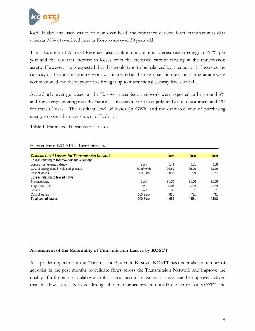
Accordingly, average losses on the Kosovo transmission network were expected to be around 3% and for energy entering into the transmission system for the supply of Kosovo customers and 1% for transit losses. The resultant level of losses (in GWh) and the estimated cost of purchasing energy to cover them are shown in Table 1.

Table 1: Estimated Transmission Losses

Extract from ESTAPIII Tariff project.

Calculation of Losses for Transmission Network 2007 2008 2009Losses relating to Kosovo demand & supplyLosses from energy balance GWh 144 151 158Cost of energy used in calculating losses Euro/MWh 26.80 25.20 23.90Cost of losses - 000 Euro 3,852 3,799 3,777Losses relating to transit flowsTransit energy GWh 3,100 3,100 3,100Target loss rate % 1.0% 1.0% 1.0%Losses GWh 31 31 31Cost of losses - 000 Euro 831 781 741Total cost of losses 000 Euro 4,683 4,581 4,518

Assessment of the Materiality of Transmission Losses by KOSTT

As a prudent operator of the Transmission System in Kosovo, KOSTT has undertaken a number of activities in the past months to validate flows across the Transmission Network and improve the quality of information available such that calculation of transmission losses can be improved. Given that the flows across Kosovo through the interconnectors are outside the control of KOSTT, the

5

principle focus of activity has been on putting in place arrangements to improve the calculation of losses associated with Kosovo energy balancing.

Improved Data Quality and Modelling

There have been two principle dimensions to these activities: improved data quality and an improved analysis methodology for the calculation and forecasting of annual transmission losses. In the following paragraphs each of these activities are outlined in turn;

Data Collection

The quality of data available to manage flows across the Kosovo Transmission System has improved considerably; and steps are in place to ensure that data quality continues to improve still further over coming months. KOSTT has initiated a programme to ensure that accurate interval metering (to hourly resolution capable of remote interrogation) is in place at all boundary points to the transmission network. As additional meters are commissioned information will be utilised to more accurately estimate Kosovan load dependent losses.

o Metering at Boundary Points (phase 1). Phase 1 of this project, was to install meters at all generation and interconnector boundaries. Data from this project is now being utilised in loss calculations.

o Metering at Boundary Points (phase 2). Phase 2 of this project is to implement metering at each of the transmission distribution sub-station boundaries and implement metering at the generation to transmission boundary of Kosovo A; it is anticipated that this project will be complete by the end of 2008 or the early part of 2009.

PSSE Modelling

6

KOSTT have purchased a license for and have been using PSSE to analyse transmission losses and an improved analysis methodology is being applied to calculate and forecast annual Transmission Losses. The improved methodology includes the following activities:

o More accurate improved modelling of the system annual load duration (based on actual recent historical data) when compared to typical load profiles assumed for each class of consumer;

o A better representation of system voltage profiles and MVAr flows (MVAr flows increase transmission losses) by using a power system model that calculates the voltage at every node of the network;

o A more accurate representation of resistance taking into account the actual age and condition of overhead lines and conductors; and

o A more realistic representation of transmission distribution interface giving a more accurate representation of no-load transmission losses.

Better availability of data, a better improved analitcal technique, indicate that the initial figure of 3% for Kosovon losses was a significant under estimate. Appendix 1 provides initial results from this modelling.

Reconciliation of Actual Transmission Loss Volumes

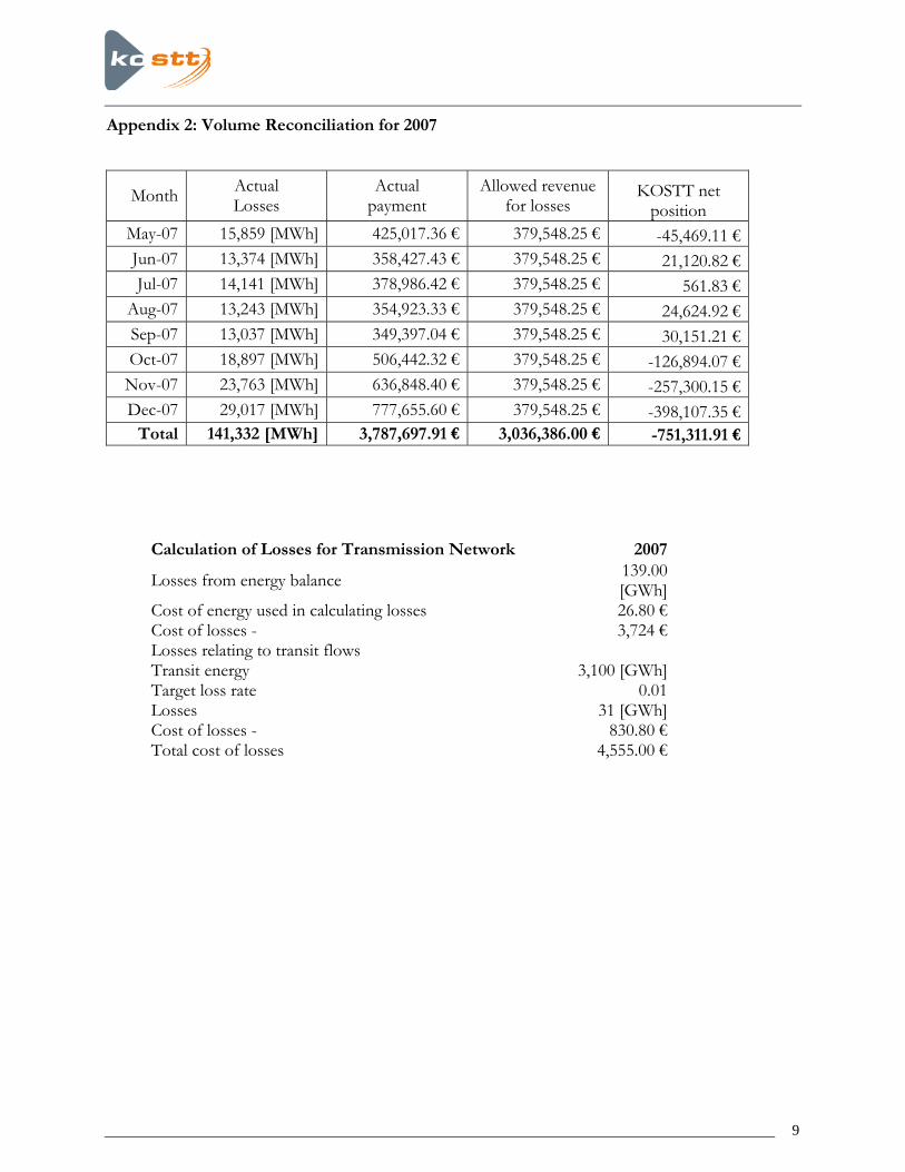
During the period the allowed revenue has been in place KOSTT have also been monitoring the volume of transmission losses and the associated costs to the business when compared to the Allowed Revenue. Attached in Appendix 2 to this paper is a table illustrating the position. The Allowed Revenue was calculated on the basis of an assumed annual volume of total losses of 175GWh. Actual data is currently only available until the end of October, however using an approximation for November and December total volumes for the year look to be in order of 259 GWh The volume is considerably greater than that anticipated at the start of the year and will have a material impact upon KOSTT’s ability to become a viable business. This information too supports our position that the initial figures assumed in the allowed revenue are too low compared to our actual position in settlements.

7

Transit Losses

It is recognised that in practise it is not possible to determine accurately which losses are associated with transit and which are associated with energy balancing within Kosovo. It is accepted that applying one loss factor for transit and a different one for domestic Kosovo demand is a reasonable approximation; provided that the cost of transit losses is a pass through. KOSTT can not control the transit flow.

It is recognised under UCTE rules that where energy transits a country there will be losses associated with this transit and that the TSO will be required to purchase energy to ensure that the volume of energy entering the country will be the same as that leaving. KOSTT recognise that it must faciltate the purchase of this energy, however, it is to this extent only that is has involvement in the transit energy flows. KOSTT has no control or influence over the volumes of transit energy and therefore it is a question whether it is appropriate for incentives to be applied transit losses.

Investment

KOSTT developed a 5 year investment plan that, in addition to improving the condition of assets on the network, would also reduce Transmission Losses to the benefit of customers. The capital projects to realise improvement in Transmission Losses are not yet commissioned due to the absence of funds to cover cuch activities. When the Allowed Revenues were set it was anticipated that some major improvements e.g. Peja 3, 400kv/110kv substation, Prizreni 2 transformer 3 installation, Pristhina 4 transformer installation, would take place in 2008/2009 and that this would compensate for anticipated increases in demand over the period. The delay in funding for such projects will increase the materiality of transmission losses over the period leading to further financial exposure to KOSTT; this again supports the position that adjustments should be made to the Allowed Revenue.

Re-opening of Allowed Revenue for Transmission Losses

As noted by ERO when the Allowed Revenue for Transmission Losses waere agreed there were a number of uncertainties associated with the current Kosova environment which could place significant risks on the TSO. It was recognised that at the time that the Allowed Revenues were set, certain assumptions were made in the absence of supporting data.

8

However, following additional evaluation, KOSTT now requests that ERO re-examine the Allowed Revenue for Transmission Losses in the following areas:

• Agree that Allowed Loss Level for Kosova Energy Balancing be reset at 4.1% for the period 2008/2009;

• Recognise that KOSTT has made payments for the purchase of Transmission Losses over and above the Allowed Revenue for 2007 and recompense KOSTT for that over payment through an additional revised allowable revenue for 2008; and

• Recognise that volume of Transit Losses is outside the direct control of KOSTT and put in place a reconciliation mechanism that allows the Allowed Revenue to be adjusted when the actual volumes of transit losses vary outside the 1% used to set the allowed revenue. This mechanism would also operate when the actual volume of transit losses is less than anticipated ensuring that KOSTT is kept neutral to activities outside is direct control.

Appendix 1:

ESTAP ! review and PSS/E Studies 2001 – 2006 and 2007/2008/2009 (attached file Shtojca 1_Humbjet në rrjetin e transmisionit.doc)

Appendix 2:

Volume Reconciliation for 2007

Appendix 3:

Estimating Losses from Metered Data (attached file Technical Annex_031207.doc)

9

Appendix 2: Volume Reconciliation for 2007

Month Actual Losses

Actual payment

Allowed revenue for losses

KOSTT net position

May-07 15,859 [MWh] 425,017.36 € 379,548.25 € -45,469.11 €Jun-07 13,374 [MWh] 358,427.43 € 379,548.25 € 21,120.82 €Jul-07 14,141 [MWh] 378,986.42 € 379,548.25 € 561.83 €

Aug-07 13,243 [MWh] 354,923.33 € 379,548.25 € 24,624.92 €Sep-07 13,037 [MWh] 349,397.04 € 379,548.25 € 30,151.21 €Oct-07 18,897 [MWh] 506,442.32 € 379,548.25 € -126,894.07 €

Nov-07 23,763 [MWh] 636,848.40 € 379,548.25 € -257,300.15 €Dec-07 29,017 [MWh] 777,655.60 € 379,548.25 € -398,107.35 €

Total 141,332 [MWh] 3,787,697.91 € 3,036,386.00 € -751,311.91 €

Calculation of Losses for Transmission Network 2007

Losses from energy balance 139.00 [GWh]

Cost of energy used in calculating losses 26.80 € Cost of losses - 3,724 € Losses relating to transit flows Transit energy 3,100 [GWh] Target loss rate 0.01 Losses 31 [GWh] Cost of losses - 830.80 € Total cost of losses 4,555.00 €

10

Annex 1

HANDLING OF METHODOLOGIES DETERMINATION OF LOSSES IN TRANSMISSION NETWORK

Introduction

1. Losses of Electricity Energy losses in EES in general are classified in:

• Technical losses • Commercial losses

Technical losses are result of electromagnet processes in electro-energetic elements during transmission process and energy distribution. Commercial losses are result of not ideal organization of system exploitation, illegal connections, no accuracy of metering energy equipments, as well as result of lost energy during system break downs. Losses depend on many factors from which most important are:

• Network configuration (voltage levels, network density, location of distribution positions as well as their distance from electrical source)

• Consume • Line sections • Load daily diagram form

Therefore, level of losses in different electro-energetic system will be different. 1.1 Technical losses These losses are divided in two categories:

• Losses, not depending from load • Losses, depending from load

Losses, not depending from load, appear as a result of setting the energy system under voltage. It could be considered as constant loss although depends on voltage level that it is considered that do not have big changes. Usually these losses appear in:

- Energy transformers that differently are called losses in work without load - In lines as a process of corona effect and electricity flow through ranges of line isolators - Dielectric losses in cable

11

Losses, depending from load, are caused from energy flow of the load through EES elements that have a certain omik resistance. Value of these losses depends from square of effective value of energy of load. These losses are variable depending from load changes. Usually these losses appear in all system elements through which energy flows however more affective are in:

- Lines (losses of active energy or losses of Joule’s effect) - Transformers (losses of active energy due to energy flow in transformers windings)

2. Standard methods of losses calculation This method is used in cases of huge and complex EES. Approach to this methodology is based on these main data:

1. Consume diagram (daily, monthly or annual). 2. Active losses value in network in maximal load. 3. EES model in computer calculations.

Lot of European countries are applying the Standard Method during losses analyze. According to standard method annual losses are calculated as following:

Δ⋅Δ=Δ TPW .......... (1) Where

WΔ = annual losses of energy

PΔ = Losses of active energy during period of maximum load (peak). Peak losses PΔ is a result based on simulations with software in which EES is modeled according to known parameters of that system. ΔT = Total hours of annual losses of energy.

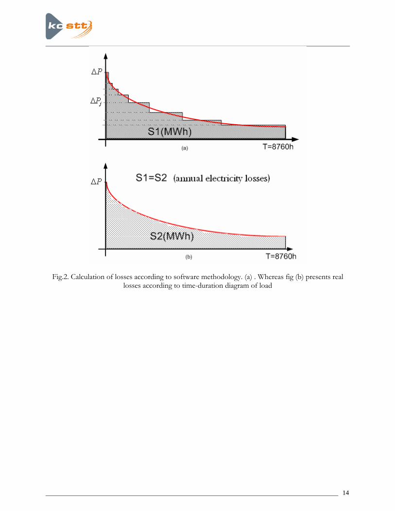
ΔT otherwise presents fictive time through which losses of energy calculated under (1) is of nods

with energy losses in normal conditions of consume change. This is presented in fig.1

12

PΔ

T=8760hΔT

PΔ

T=8760h

S1

S2

S1=S2 (annual electricity losses)

Fig.1 Understanding of total hours of annual losses of energy ΔT

The accurate expression of calculation of ΔT is as following:

2

8760

0

2

maxP

dtPT

∫=Δ ............................................. (2)

In case that annual diagram of load is known for each hour than approximate calculation of ΔT is performed as following:

2

8760

11

2

max

)(

P

ttPT j

jjj∑=

−

Δ

−⋅= .......................................... (3)

Where Pj = current consume for hour j (there are 8760 values) Pmax = maximum consume during the year that is analyzed t = time (hour)

13

3. Software method of losses calculation There is also software method of calculation of energy in EES. This method is based on losses calculation of peak for different consume. Approach to this methodology is based on these main data:

1. Consume diagram (daily, monthly or annual). 2. Active losses value in network in different loads. 3. Modeling of EES in relevant software.

As higher the number of simulations is for different loads more accurate performance of energy losses calculation will be. However, also limited number of simulations leads to sufficient results. Energy losses according to this method is calculated as following:

)( 1

8760

1−

=

−⋅Δ=Δ ∑ jjjj

ttPW .............................. (3)

Where

jPΔ = losses of active energy for different consume t = time (hour) Calculation of energy losses in relevant software is based on standard method of calculation of energy flow mainly in accordance with method of Newton - Raphson through iterative processes.

14

Fig.2. Calculation of losses according to software methodology. (a) . Whereas fig (b) presents real losses according to time-duration diagram of load

15

4. CALCULATION OF LOSSES (2001-2009) ACCORDING TO STANDARD METHODOLOGY Incoming data:

• Gross consume for 2001- 2006, 2007, 2008 and 20093 • Time-duration of load for 2001-2006, 2007, 2008 and 20094 • Kosovo EES model in PSSE for 2001- 20095

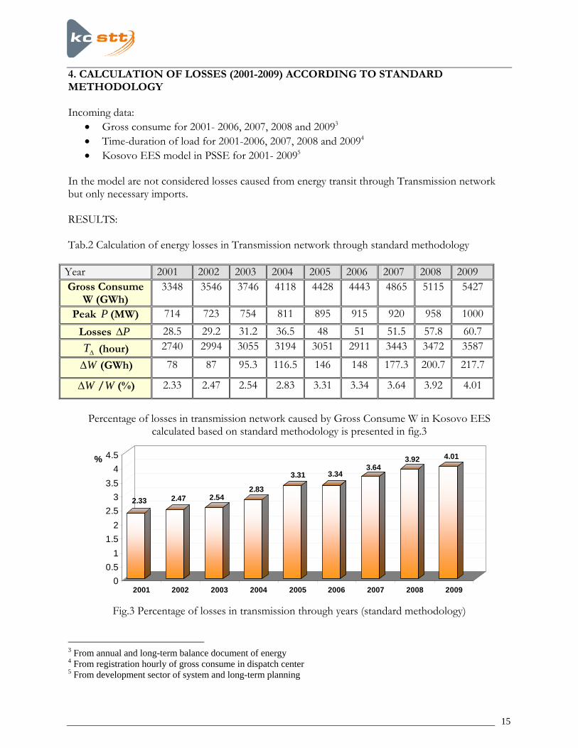
In the model are not considered losses caused from energy transit through Transmission network but only necessary imports. RESULTS: Tab.2 Calculation of energy losses in Transmission network through standard methodology

Year 2001 2002 2003 2004 2005 2006 2007 2008 2009 Gross Consume

W (GWh) 3348

3546 3746 4118 4428 4443 4865 5115 5427

Peak P (MW) 714 723 754 811 895 915 920 958 1000 Losses PΔ 28.5 29.2 31.2 36.5 48 51 51.5 57.8 60.7

ΔT (hour) 2740 2994 3055 3194 3051 2911 3443 3472 3587

WΔ (GWh) 78 87 95.3 116.5 146 148 177.3 200.7 217.7

WΔ /W (%) 2.33 2.47 2.54 2.83 3.31 3.34 3.64 3.92 4.01

Percentage of losses in transmission network caused by Gross Consume W in Kosovo EES

calculated based on standard methodology is presented in fig.3

2.33 2.47 2.542.83

3.31 3.343.64

3.92 4.01

00.5

11.5

22.5

33.5

44.5%

2001 2002 2003 2004 2005 2006 2007 2008 2009

Fig.3 Percentage of losses in transmission through years (standard methodology)

3 From annual and long-term balance document of energy 4 From registration hourly of gross consume in dispatch center 5 From development sector of system and long-term planning

16

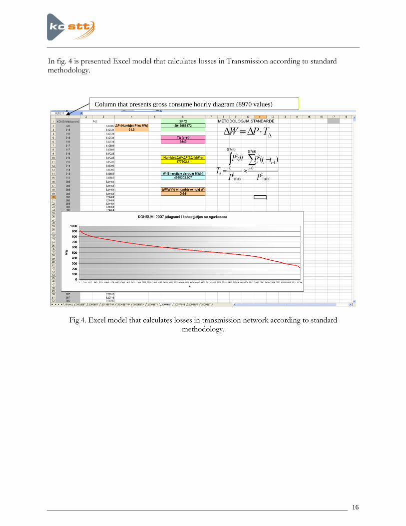
In fig. 4 is presented Excel model that calculates losses in Transmission according to standard methodology.

Fig.4. Excel model that calculates losses in transmission network according to standard methodology.

Column that presents gross consume hourly diagram (8970 values)

17

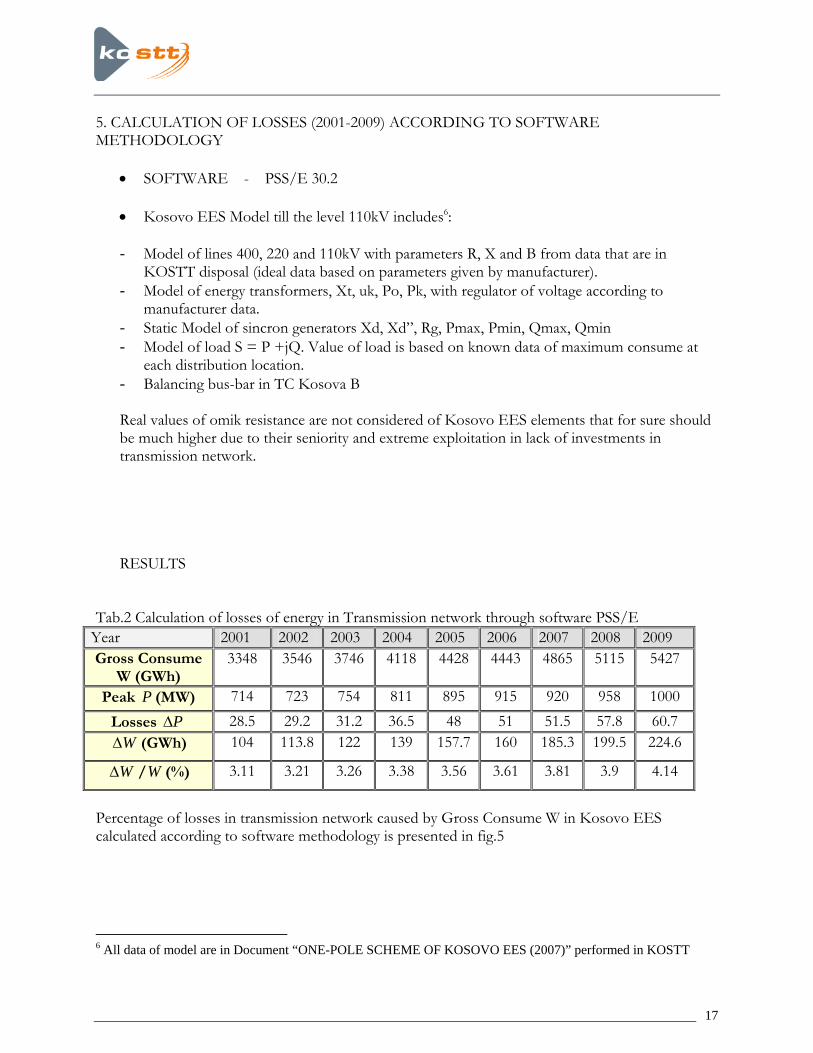
5. CALCULATION OF LOSSES (2001-2009) ACCORDING TO SOFTWARE METHODOLOGY

• SOFTWARE - PSS/E 30.2 • Kosovo EES Model till the level 110kV includes6: - Model of lines 400, 220 and 110kV with parameters R, X and B from data that are in

KOSTT disposal (ideal data based on parameters given by manufacturer). - Model of energy transformers, Xt, uk, Po, Pk, with regulator of voltage according to

manufacturer data. - Static Model of sincron generators Xd, Xd”, Rg, Pmax, Pmin, Qmax, Qmin - Model of load S = P +jQ. Value of load is based on known data of maximum consume at

each distribution location. - Balancing bus-bar in TC Kosova B Real values of omik resistance are not considered of Kosovo EES elements that for sure should be much higher due to their seniority and extreme exploitation in lack of investments in transmission network. RESULTS

Tab.2 Calculation of losses of energy in Transmission network through software PSS/E

Year 2001 2002 2003 2004 2005 2006 2007 2008 2009 Gross Consume

W (GWh) 3348

3546 3746 4118 4428 4443 4865 5115 5427

Peak P (MW) 714 723 754 811 895 915 920 958 1000 Losses PΔ 28.5 29.2 31.2 36.5 48 51 51.5 57.8 60.7

WΔ (GWh) 104 113.8 122 139 157.7 160 185.3 199.5 224.6

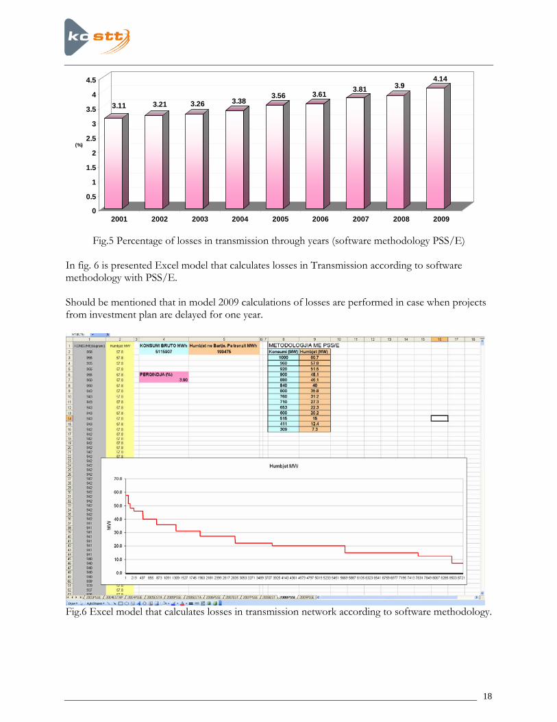
WΔ /W (%) 3.11 3.21 3.26 3.38 3.56 3.61 3.81 3.9 4.14

Percentage of losses in transmission network caused by Gross Consume W in Kosovo EES calculated according to software methodology is presented in fig.5

6 All data of model are in Document “ONE-POLE SCHEME OF KOSOVO EES (2007)” performed in KOSTT

18

3.11 3.21 3.26 3.383.56 3.61 3.81 3.9

4.14

0

0.5

1

1.5

2

2.5

3

3.5

4

4.5

(%)

2001 2002 2003 2004 2005 2006 2007 2008 2009

Fig.5 Percentage of losses in transmission through years (software methodology PSS/E)

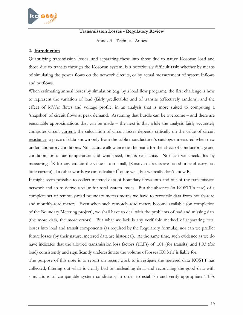
In fig. 6 is presented Excel model that calculates losses in Transmission according to software methodology with PSS/E. Should be mentioned that in model 2009 calculations of losses are performed in case when projects from investment plan are delayed for one year.

Fig.6 Excel model that calculates losses in transmission network according to software methodology.

19

Transmission Losses - Regulatory Review

Annex 3 - Technical Annex

2. Introduction

Quantifying transmission losses, and separating these into those due to native Kosovan load and

those due to transits through the Kosovan system, is a notoriously difficult task: whether by means

of simulating the power flows on the network circuits, or by actual measurement of system inflows

and outflows.

When estimating annual losses by simulation (e.g. by a load flow program), the first challenge is how

to represent the variation of load (fairly predictable) and of transits (effectively random), and the

effect of MVAr flows and voltage profile, in an analysis that is more suited to computing a

‘snapshot’ of circuit flows at peak demand. Assuming that hurdle can be overcome – and there are

reasonable approximations that can be made – the next is that while the analysis fairly accurately

computes circuit current, the calculation of circuit losses depends critically on the value of circuit

resistance, a piece of data known only from the cable manufacturer’s catalogue measured when new

under laboratory conditions. No accurate allowance can be made for the effect of conductor age and

condition, or of air temperature and windspeed, on its resistance. Nor can we check this by

measuring I2R for any circuit: the value is too small, (Kosovan circuits are too short and carry too

little current). In other words we can calculate I2 quite well, but we really don’t know R.

It might seem possible to collect metered data of boundary flows into and out of the transmission

network and so to derive a value for total system losses. But the absence (in KOSTT’s case) of a

complete set of remotely-read boundary meters means we have to reconcile data from hourly-read

and monthly-read meters. Even when such remotely-read meters become available (on completion

of the Boundary Metering project), we shall have to deal with the problems of bad and missing data

(the more data, the more errors). But what we lack is any verifiable method of separating total

losses into load and transit components (as required by the Regulatory formula), nor can we predict

future losses (by their nature, metered data are historical). At the same time, such evidence as we do

have indicates that the allowed transmission loss factors (TLFs) of 1.01 (for transits) and 1.03 (for

load) consistently and significantly underestimate the volume of losses KOSTT is liable for.

The purpose of this note is to report on recent work to investigate the metered data KOSTT has

collected, filtering out what is clearly bad or misleading data, and reconciling the good data with

simulations of comparable system conditions, in order to establish and verify appropriate TLFs

20

applicable to the current Regulatory period. The Consultant considers that the approach developed

here, in combination with the more accurate measurements available once the Boundary Metering

project is completed, provides a sounder and more verifiable basis for the future monitoring of

losses and the estimation of TLFs than any considered so far.

3. Estimating Annual Losses by the ‘Standard’ Method

To describe the modelling approach adopted in ESTAP 1 (Module D) as an ‘industry standard’ is

perhaps a bit of stretch. It is certainly a convenient and quick proxy for a more comprehensive

analysis of losses, and gives a forecast of annual losses based on a single study at peak which, given

the almost total lack of data at the time the work was carried out (pre-2002), was probably the only

viable approach to take.

To compensate for the lack of data, the authors of the ESTAP I report had to make some crucial

assumptions about the forecast load: in particular the shape of the load duration curve (about which

they had no hard data, and which they were forced to construct from consideration of the likely

proportion and profile of the various classes of load in Kosova), and also to estimate the peak load

in any given year. Also, their chosen analytic approach takes no account of the effect on losses of

changes in voltage profile and the resulting MVAr flow at different load levels, which is very

significant in the Kosovan system because of the heavy loading of 110kV circuits and distribution

transformers. On the contrary, they assume a constant power factor. Finally, their calculation of

losses at peak uses the ‘catalogue’ value of circuit resistance, in spite of the age and condition of

many conductors.

Nevertheless, the analysis of Kosovan losses in ESTAP I is a creditable effort, given the limited

knowledge the authors had of actual network conditions and system load. With more accurate data

on the shape of the load duration curve and a more recent forecast of peak load, the ‘standard’

approach can give a reasonable estimate of annual losses, but only if the computation of losses at

peak makes due allowance for the increased resistance of old conductors in poor condition. This

has been done, giving the results tabulated below.

4. An Improved Method of Calculating Annual Losses

KOSTT’s System Development and Long-Term Planning section have lately developed an

alternative approach using the power system simulation programme, PSS/E. The approach

combines multiple loadflows at several demand levels which collectively form a multi-level

approximation to the load duration curve using on recent data and weighting the results according to

21

the hours at each level, together with more accurate modelling of the transmission/distribution

interface transformers (to represent their no-load losses) and of the voltage profile and MVAr flows

at each load level. The network model also uses a more realistic estimate of circuit resistances taking

account of their age and condition.

This analysis, applied to the years 2007-09, produced the estimates of annual losses for 2007-09

tabulated below.

5. Estimating Losses from Metered Data

5.1 General Description

KOSTT presently collects hourly metered data on interconnector flows and generator ‘gross’

production (i.e. excluding the generators’ self-supply of load). But they do not yet have hourly

metered data on the demand side: these meters are read only monthly. Thus we cannot directly

compare system inflows and outflows, and correlate these to analyse the variation of losses with

transit and Kosovan demand and so derive the actual TLFs.

Nevertheless it is possible, in the interim, to analyse the data we have available and – making some

reasonable assumptions as to the dependency of total losses on transit and demand – to develop a

model of losses that allows us to make a good estimate of the TLFs, which can at the very least be

used to calibrate the PSSE-based analysis.

The procedure we have developed is described below, and should be read with reference to the

diagram below.

From the hourly data on gross generation and the monthly meter readings of generation (self-

supplied) demand, we estimate ‘net’ hourly generation production – assuming each generator in each

22

month absorbs the same fraction of its gross output7. Adding to this the net hourly import from

interconnectors (Ih-Xh), we obtain an estimate of hourly ‘gross’ import to the transmission system

(which equals net demand plus total losses).

Then, from the monthly meter readings of demand at all grid supply points (GSPs)8 on the

transmission network, we can derive an estimate for the hourly aggregate net GSP demand,

assuming this has approximately the same profile as gross transmission import. The difference

between these gives an estimate of the total transmission losses (due to both transit and to Kosovan

load) in each hour.

5.2 Analysis of Hourly Loss Data

The overall objective of this step is to extract estimates of the load and transit TLFs from the

available data (all of 2006, and January-October 2007).

Applying multiple linear regression analysis to each complete set of data produces a very confusing

result. Whereas for 2006 we get seemingly reasonable TLFs of 1.079 for load and 1.016 for transit,

for 2007 we get respectively 1.087 and 0.966 – which implies that increasing transit reduces Kosovan

losses, a physical impossibility given the structure of the present Kosovan network.

Examination of the data on a week-by-week basis indicates the likely source of the problem. In

2006, there are many weeks where the hourly load data shows little evidence of a periodic daily

profile, even taking into account the peak-lopping effect of the ABC load-management scheme.

The TLF for load, whilst surprisingly high at around 1.08, varies widely (1.05 to 1.12) without

showing any particular pattern (we discount the 4-week blocks: this is a consequence of inputting

data monthly). All of these factors point toward the presence of ‘bad’ data9 in the measurements:

consequently we do not believe the results for 2006 can be relied upon.

Data for the first three months of 2007 show similar signs of bad data. Although the daily load

profiles for this period look more credible, the consistently high value of load TLF looks very

7 It would have been better to estimate net hourly production for each individual generating unit, netting off its monthly metered

demand from its monthly gross output to scale back the hourly figures, then summating these across all units. No such breakdown of generation data was available for this analysis, but the approximation noted above does not materially affect the outcome. Nevertheless, this approach is recommended for future analyses.

8 Note, that as the Boundary Metering project progresses, we can substitute actual GSP hourly metered data into this step, gradually improving the quality of the estimate of hourly aggregate net GSP demand in future analyses.

9 One of the problems with any data collection system is that errors, both systematic and random, are also collected and that some data will be misread or dropped. Any SCADA/EMS system will incorporate feature to automatically detect and rectify bad or missing data. Lacking this, all we can do at present is apply a ‘sense-check to the data we have.

23

suspect, as does its sudden drop from 1.08 on 31/3/2007 to 1.03 on 1/4/2007. Further enquiry

uncovered some facts that helped to explain this discrepancy:-

On that date, the ‘boundary’ of the metering system was changed to exclude the 110/X kV

distribution transformers. All previous measurements had included the losses of these

transformers (which helps explain the exceptionally high TLF from January 2006 to March

2007) and, while we might be able to estimate a correction to remove their effect, that is not

our primary aim.

On the same date, all boundary meters were checked and re-sealed.

Previous to that date, there had been several changes to the network, with extended circuit

outages and GSPs connected at different points on the network.

All of these factors make meter readings up to and including March 2007 suspect. If they were to be

included in the TLF analysis, we consider they would artificially and wrongly inflate the resulting

TLF for load. We have therefore excluded them.

The data for October 2007 is also suspect, but we think there is a different factor at work here.

Apparently a new set of monthly meter readings has introduced an error that has distorted the

results for this month (one of the hazards of manually logged readings). It might be that November

and December data, when available, will corroborate or correct this last set of data, and bring their

results more into line with those for April to September. However, for the present, we consider

October’s data are best discounted.

5.3 Analysis of ‘Good’ Loss Data: April-September 2007

Multiple linear regression analysis of this portion of data gives estimated TLFs of 1.038 for load.This

is significantly higher than the 1.03 allowed in the Price Control.

To see how losses vary with transit and load, we examined the April-September data in various ways.

The first thing to note is the random nature of transit flows, which is no surprise, as the flows on the

interconnector circuits are very much outside of KOSTT’s control.

Histogram of TransitsApr-Sep 2007

0%

2%

4%

6%

8%

10%

12%

0

139

199

259

319

379

439

499

559

619

679

24

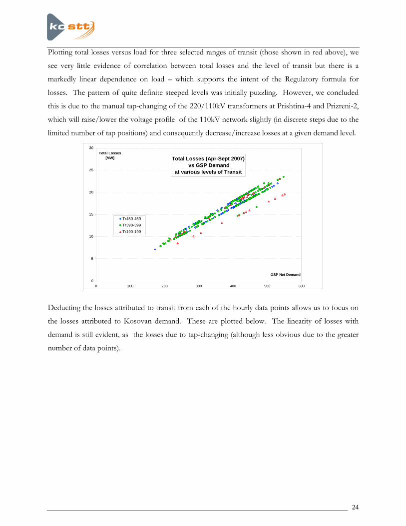
Plotting total losses versus load for three selected ranges of transit (those shown in red above), we

see very little evidence of correlation between total losses and the level of transit but there is a

markedly linear dependence on load – which supports the intent of the Regulatory formula for

losses. The pattern of quite definite steeped levels was initially puzzling. However, we concluded

this is due to the manual tap-changing of the 220/110kV transformers at Prishtina-4 and Prizreni-2,

which will raise/lower the voltage profile of the 110kV network slightly (in discrete steps due to the

limited number of tap positions) and consequently decrease/increase losses at a given demand level.

Total Losses (Apr-Sept 2007) vs GSP Demand

at various levels of Transit

0

5

10

15

20

25

30

0 100 200 300 400 500 600

GSP Net Demand

Total Losses[MW]

Tr450-459Tr390-399Tr190-199

Deducting the losses attributed to transit from each of the hourly data points allows us to focus on

the losses attributed to Kosovan demand. These are plotted below. The linearity of losses with

demand is still evident, as the losses due to tap-changing (although less obvious due to the greater

number of data points).

25

Losses due to Kosova GSP DemandApr-Sept 2007

y = 3.76%x

y = 4.25%x

y = 3.19%x

y = 3%x

0

5

10

15

20

25

30

35

40

0 100 200 300 400 500 600 700 800

GSP Net Demand

Loss[MW]

What is more significant is that the best-fit straight line passing through all data points has a slope of

3.76%, and that the measured data are bounded by lines with slopes of 3.19% and 4.25%. That is to

say, the measured TLF for load has a value that lies between 1.0319 and 1.0425 with a mean of

1.0376. The red line representing the allowed TLF of 1.03 passes below all but a very few points.

Given that data for the summer months only has been used in this analysis and given that demand

for the winter months (January to March and October to December) would have produced many

more data points between 600 and 900MW that, on this evidence, would have contributed higher

losses, it seems clear that the allowed TLF of 1.03 significantly underestimates the volume (and cost)

of losses that KOSST is liable for.

5.4 Calibrating Loss Simulations

Using the load duration curve for the April-September load data, KOSTT has simulated the losses

due to Kosovan load by the standard and PSSE methodologies described above. They then adjusted

the resistance values of old 110kV circuits known (identified in earlier work by the Consultants) to

be in poor condition and more lossy than the average, so that the simulated losses for April-

September align with those measured. The resulting network values were then used to predict full-

year losses due to serving Kosovan demand for 2007-09, as shown in the table below.

Standard method PSSE method

Year

Kosovan demand supplied [GWh]

Losses at Allowed TLF of

1.03 Estimated

losses [GWh]

TLF(load)Estimated

losses [GWh]

TLF(load)

26

2007 4865 146.0 177.3 1.036 185.3 1.038

2008 5115 153.5 200.7 1.039 199.5 1.039

2009 5427 162.8 217.7 1.040 224.6 1.041 Total 2007-09 15407 462.2 595.7 1.039 609.4 1.041

6. Conclusions

6.1 Both Standard and PSSE simulation methods give practically the same result when applied

to more recent data on the Kosovan load duration curve and a more recent projection of

load growth than was the case in the ESTAP I report, and when the analysis uses a more

realistic value for some circuit resistances.

6.2 The PSSE simulation is considered to give slightly more accurate results than the Standard

method (principally because it takes into account variations in MVAR flow and voltage

profile at different demand levels, which the Standard method does not). And this is

corroborated by an analysis of good-quality metered data collected between April and

September 2007.

6.3 All of the analyses carried out by KOSTT and their Consultants predict that the losses

attributable to load will turn out to be substantially greater than what was expected in the

2007-09 Price Control. The excess is estimated at 147,200MWh over the three-year period,

at an extra cost to KOSTT of around €3.7M over the portion of their allowed revenue that

was allocated to pay for losses. This surcharge, if not quickly addressed, will impose a

significant financial burden on KOSTT that will both threaten their viability as a business,

and will materially affect their ability to invest to improve the security and quality of supply.

(End)