Transmembrane helices predicted at 95% accuracy

Protein Science (1995), 4:521-533. Cambridge University Press. Printed in the USA. Copyright 0 1995 The Protein Society

Transmembrane helices predicted at 95 Yo accuracy

BURKHARD ROST,’ RITA CASAD10,2 PIER0 FARISELLI,2 AND CHRIS SANDER’ ’ Protein Design Group, EMBL Heidelberg, 69 012 Heidelberg, Germany

Laboratory of Biophysics, Department of Biology, University of Bologna, 40 126 Bologna, Italy (RECEIVED October 31, 1994; ACCEPTED December 29, 1994)

Abstract

We describe a neural network system that predicts the locations of transmembrane helices in integral membrane proteins. By using evolutionary information as input to the network system, the method significantly improved on a previously published neural network prediction method that had been based on single sequence information. The input data were derived from multiple alignments for each position in a window of 13 adjacent residues: amino acid frequency, conservation weights, number of insertions and deletions, and position of the window with re- spect to the ends of the protein chain. Additional input was the amino acid composition and length of the whole protein. A rigorous cross-validation test on 69 proteins with experimentally determined locations of transmem- brane segments yielded an overall two-state per-residue accuracy of 95%. About 94% of all segments were pre- dicted correctly. When applied to known globular proteins as a negative control, the network system incorrectly predicted fewer than 5% of globular proteins as having transmembrane helices. The method was applied to all 269 open reading frames from the complete yeast VI11 chromosome. For 59 of these, at least two transmembrane helices were predicted. Thus, the prediction is that about one-fourth of all proteins from yeast VI11 contain one transmembrane helix, and some 20’70, more than one.

Keywords: evolutionary information; integral membrane proteins; multiple alignments; neural networks; pro- tein structure prediction; secondary structure; yeast VI11 chromosome

Given the rapid advance of large-scale gene-sequencing projects (Oliver et al., 1992; Johnston et al., 1994), most protein se- quences of key organisms will be known in about 5 years’ time. Experimental structure determination is becoming more of a routine (Lattman, 1994); and the number of proteins with known sequence for which the three-dimensional (3D) structure can be predicted rather accurately by homology modeling is con- stantly increasing (today more than 25% of all sequences in the SWISS-PROT sequence data base [Bairoch & Boeckmann, 19941 can be modeled with reasonable accuracy by homology [Sander & Schneider, 19941). Even in such an optimistic sce- nario, experimental knowledge about membrane proteins is likely to be sparse. However, membrane proteins represent a very important class of protein structures. To what extent can structural aspects for membrane proteins be predicted from se- quence information?

Two types of rnembraneproteins. So far, the 3D structures of two types of membrane proteins have been determined. The first type are helical proteins: photosynthetic reaction center (Deisenhofer et al., 1985), bacteriorhodopsin (Henderson et al.,

Reprint requests to: Burkhard Rost, Protein Design Group, EMBL Heidelberg, 69 012 Heidelberg, Germany; e-mail: rost@embl-heidelberg. de.

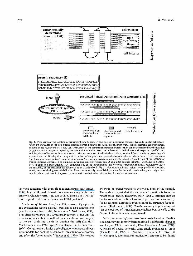
1990), and the light harvesting complex I1 (Wang et al., 1993; Kuhlbrandt et al., 1994); these proteins consist of typically apo- lar helices of some 20 residues that traverse the membrane per- pendicular to its surface (Fig. 1). The second type is represented by the structure of porin (Weiss & Schulz, 1992; Cowan & Rosenbusch, 1994), a 16-stranded /3-barrel.

Membrane proteins easier to predict than globular ones. Typ- ical methods for the prediction of transmembrane segments focus on helical transmembrane (HTM) proteins (von Heijne, 1981, 1986; Argos et al., 1982; Eisenberg et al., 1984a; Engel- man et al., 1986; von Heijne & Gavel, 1988). It is commonly be- lieved that the prediction of structure is simpler for membrane proteins than for globular ones as the lipid bilayer imposes strong constraints on the degrees of freedom of structure (Taylor et al., 1994).

Prediction of transmembrane segments. Methods for predic- tion of transmembrane helices are usually based on (1) hydro- phobicity analyses (Argos et al., 1982; Kyte & Doolittle, 1982; Engelman et al., 1986; Cornette et al., 1987; Degli Esposti et al., 1990); (2) the preponderance of positively charged residues on the cytoplasmic side of the transmembrane segment (interior), established as the “positive inside rule” (von Heijne, 1981, 1986, 1991, 1992; von Heijne & Gavel, 1988; Sipos & von Heijne, 1993); or (3) statistical procedures that perform significantly bet-

521

522 B. Rost et al.

protein sequence (1D) FHEPIWIAGI ILGLALVGLITYFGKWI‘YLWLWLTS VDHKR~IMYITVAIVMLL~FADAIMMRSQQA~SAGEA GnPPHHMOIFTAHGVlMIFNAMPFVIGZMNLVVPLOI

Fig. 1. Prediction of the location of transmembrane helices. In one class of membrane proteins, typically apolar helical seg- ments are embedded in the lipid bilayer oriented perpendicular to the surface of the membrane. Helical segments can be regarded as more or less rigid cylinders. Thus, the 3D structure of the membrane spanning protein region can be determined by: the location of segments with respect to sequence; the orientation of helical axes; the inclination of helical axes with respect to lipid bilayer; and the phase of helices with respect to each other (orientation of helical wheel). Here, we simplify extremely by projecting 3D structure onto a 1D string describing which residues of the protein are part of a transmembrane helices. Input to the prediction tool (neural network system) is a protein sequence (in general a sequence alignment), output is a prediction of the location of transmembrane segments. The example shown (sequence of cytochrome 0 ubiquinol oxidase subunit I , cyob-eco in SWISS- PROT; Bairoch & Boeckmann, 1994) contained one of the few segments that were underpredicted (missed). The numbers give the reliability of the prediction for each residue on a scale of 0-9 (Fig. 2). Nontransmembrane regions, when predicted correctly, usually reached the highest reliability (9). Thus, the unusually low reliability values for the underpredicted segment might have enabled the expert user to improve the automatic prediction by interpreting this region as nonloop.

ter when combined with multiple alignments (Persson & Argos, 1994). In general, prediction of transmembrane segments is rel- atively straightforward. But, can detailed aspects of 3D struc- ture be predicted from sequence for HTM proteins?

Prediction of 3 0 structure for HTMproteins. Cytoplasmic and extracellular regions have different amino acid compositions (von Heijne & Gavel, 1988; Nakashima & Nishikawa, 1992). This difference allows for a successful prediction of not only the location of helices but, as well, of their orientation with respect to the cell (pointing inside or outside the cell) (Landolt- Marticorena et al., 1992; Sipos & von Heijne, 1993; Jones et al., 1994). Going further, Taylor and colleagues enumerate all pos- sible models for packing seven-helix transmembrane proteins and select the “better models” (Taylor et al., 1994). The selection

criterion for “better models” is the crucial point of the method. The authors report that the native conformation is found in “most cases” tested. However, the N- and C-terminal ends of the transmembrane helices have to be predicted very accurately for a successful automatic prediction of 3D structure from se- quence (Taylor et al., 1994). Can the accuracy of predicting not just the location of transmembrane helices but, as well, of the N- and C-terminal ends be improved?

Better prediction of transmembrane helix location. Predic- tion accuracy has recently been improved significantly (Sipos & von Heijne, 1993; Jones et al., 1994; Persson & Argos, 1994). A system of neural networks using single sequences as input (Fariselli et al., 1993; R. Casadio, P. Fariselli, C. Taroni, & M. Compiani, submitted for publication) appears to be slightly

Transmembrane helices predicted 523

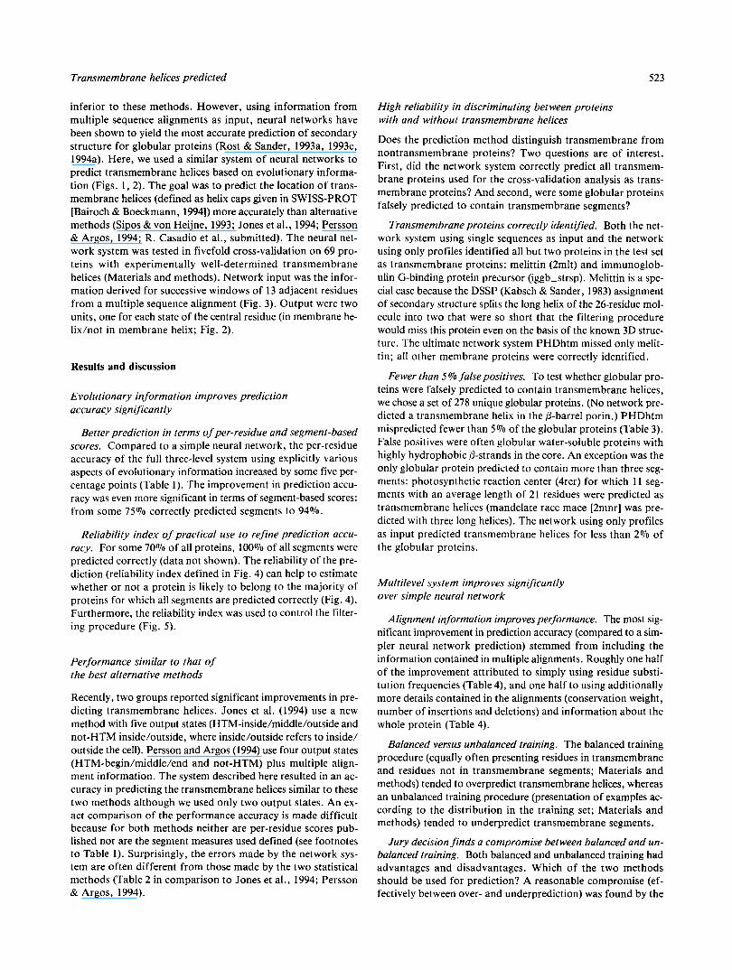
inferior to these methods. However, using information from High reliability in discriminating between proteins multiple sequence alignments as input, neural networks have with and without transmembrane helices been shown to yield the most accurate prediction of secondary structure for globular proteins (Rost & Sander, 1993a, 1993c, 1994a). Here, we used a similar system of neural networks to predict transmembrane helices based on evolutionary informa- tion (Figs. l , 2). The goal was to predict the location of trans- membrane helices (defined as helix caps given in SWISS-PROT [Bairoch & Boeckmann, 19941) more accurately than alternative methods (Sipos & von Heijne, 1993; Jones et al., 1994; Persson & Argos, 1994; R. Casadio et al., submitted). The neural net- work system was tested in fivefold cross-validation on 69 pro- teins with experimentally well-determined transmembrane helices (Materials and methods). Network input was the infor- mation derived for successive windows of 13 adjacent residues from a multiple sequence alignment (Fig. 3). Output were two units, one for each state of the central residue (in membrane he- lix/not in membrane helix; Fig. 2).

Results and discussion

Evolutionary information improves prediction accuracy significantly

Better prediction in terms of per-residue and segment-based scores. Compared to a simple neural network, the per-residue accuracy of the full three-level system using explicitly various aspects of evolutionary information increased by some five per- centage points (Table 1). The improvement in prediction accu- racy was even more significant in terms of segment-based scores: from some 75% correctly predicted segments to 94%.

Reliability index of practical use to refine prediction accu- racy. For some 70% of all proteins, 100% of all segments were predicted correctly (data not shown). The reliability of the pre- diction (reliability index defined in Fig. 4) can help to estimate whether or not a protein is likely to belong to the majority of proteins for which all segments are predicted correctly (Fig. 4). Furthermore, the reliability index was used to control the filter- ing procedure (Fig. 5 ) .

Performance similar to that of the best alternative methods

Recently, two groups reported significant improvements in pre- dicting transmembrane helices. Jones et al. (1994) use a new method with five output states (HTM-inside/middle/outside and not-HTM inside/outside, where inside/outside refers to inside/ outside the cell). Persson and Argos (1994) use four output states (HTM-begin/middie/end and not-HTM) plus multiple align- ment information. The system described here resulted in an ac- curacy in predicting the transmembrane helices similar to these two methods although we used only two output states. An ex- act comparison of the performance accuracy is made difficult because for both methods neither are per-residue scores pub-

Does the prediction method distinguish transmembrane from nontransmembrane proteins? Two questions are of interest. First, did the network system correctly predict all transmem- brane proteins used for the cross-validation analysis as trans- membrane proteins? And second, were some globular proteins falsely predicted to contain transmembrane segments?

Transmembrane proteins correctly identifed. Both the net- work system using single sequences as input and the network using only profiles identified all but two proteins in the test set as transmembrane proteins: melittin (2mlt) and immunoglob- ulin G-binding protein precursor (iggb-strsp). Melittin is a spe- cial case because the DSSP (Kabsch & Sander, 1983) assignment of secondary structure splits the long helix of the 26-residue mol- ecule into two that were so short that the filtering procedure would miss this protein even on the basis of the known 3D struc- ture. The ultimate network system PHDhtm missed only melit- tin; all other membrane proteins were correctly identified.

Fewer than 5% falsepositives. To test whether globular pro- teins were falsely predicted to contain transmembrane helices, we chose a set of 278 unique globular proteins. (No network pre- dicted a transmembrane helix in the 0-barrel porin.) PHDhtm mispredicted fewer than 5% of the globular proteins (Table 3). False positives were often globular water-soluble proteins with highly hydrophobic 0-strands in the core. An exception was the only globular protein predicted to contain more than three seg- ments: photosynthetic reaction center (4rcr) for which 11 seg- ments with an average length of 21 residues were predicted as transmembrane helices (mandelate race mace [2mnr] was pre- dicted with three long helices). The network using only profiles as input predicted transmembrane helices for less than 2% of the globular proteins.

Multilevel system improves significantly over simple neural network

Alignment information improves performance. The most sig- nificant improvement in prediction accuracy (compared to a sim- pler neural network prediction) stemmed from including the information contained in multiple alignments. Roughly one half of the improvement attributed to simply using residue substi- tution frequencies (Table 4), and one half to using additionally more details contained in the alignments (conservation weight, number of insertions and deletions) and information about the whole protein (Table 4).

Balanced versus unbalanced training. The balanced training procedure (equally often presenting residues in transmembrane and residues not in transmembrane segments; Materials and methods) tended to overpredict transmembrane helices, whereas an unbalanced training procedure (presentation of examples ac- cording to the distribution in the training set; Materials and methods) tended to underpredict transmembrane segments.

lished nor are the segment measures used defined (see footnotes Jury decision finds a compromise between balanced and un- to Table 1). Surprisingly, the errors made by the network sys- balanced training. Both balanced and unbalanced training had tem are often different from those made by the two statistical advantages and disadvantages. Which of the two methods methods (Table 2 in comparison to Jones et al., 1994; Persson should be used for prediction? A reasonable compromise (ef- & Argos, 1994). fectively between over- and underprediction) was found by the

524 B. Rosl el al.

- g

%

3

m (I] A

3 - c) C - -3 C

CI 0 m '3 > 0

0

- - 3 d

4 c " 8 E 2 503 2 2 .- .n

s z .c 8 = a gz 52 & O

zg 2 3 r; .E = a 2cJ GI- 2 E c

.o 3 c d .- 23 e c c *s 9 2 2 a ? E gg

.-

m

2 E : g T Z . z g2 E s j : .o 873 3x;zx.ozb " C L & L . 532 e, 2 0 E $'.!2r . - - e - -2- m e, 0 c m m mXz 3 L L:=-

O Z " m 2 2.5 I z 5 : 2 o o - o , p A G 2 E 02.2- Q 3 z 5 r - o - S L + g u - z $z.g 8sZ.g ;$== , + ~ g J c s s : ; 5 2 2 82 z.J-.rz.r: $<2&?.; ec.gs2 z g ; 2 p : 2 z o a J [gg 3 g.?+ m E s L

aL.2 3 ,S?;.; $:G c K + c&c,-, z 5 . g g . g g s ~ s ; f ~ ~ . 3.ZiSz.s L. a ~ z -

c 2 3 .- .- s c o e , e , c - " g ~ , ~ c c aJ-5z u; 8 2 2

l 5 . 5 V s $+.*c : z .- u z k - 5 t L.u e, 04 z G ; 3 $ - J c c * z 3 . g .- L v c e, c a g j + , - ; e, k;Cr,'* aJ

gLL.;":.".' c aJ m * + u g D 0 aJ aJ2 c c w -

A.s .; 3 - 8 ,o ;a - aJ 04- a's oz V) 0 m X ?, m m 2 c czL g ? e 3.- aJ- - QJ.- O U g.z A C r, :u .%cg 2.E.E -"S gu m .- C:dsg{z,L%a$E c 9 ; - g Zj z.5 2 2 8 z

c s c ! c e , -

x g C = : 1 E z 5

U . - U E D 0-

e , S Z 0 L 0

c-'cI 0 c 0 - gzMZ 11 = U E a, v L

5 gs gi'Z;a E e,.=+

5 5 J ; c c g p $ . g e - g 0 - 3 E22 2:Z.E

Zrn

o m - - .- .- - =@ M ;g5 - A ? 2g 3 P " t . 2 % E 0 c: c L n 2 5 . 0 2 - L g O z L a;o

5 . 5 . - - 2 u 2 - m a , ~ u ~ . 5 a J o ' g u o a m c 8 . ~ c , r ; % ,:5 05 -2 aJ LI? e 2 g m

= 2 g 0 u:z A255 E E

L" I,"..'& 8 g 3 &:x 0%; 0.5 3 0 m O 2 . G U ' O Z % S i 2 LaJ m T30" & a c m . 2 i f . c aJ m 2 :: 8 2 , - 2 2 ~ 0 ! G ; s ~ ~

58:Ig&;p;$

2 2 g.g 2 ? . 2 5 Z % Y.2

" 9 " o s i ; s g ; m c c e & L. 02;5 % 0 $3soczo - L Z S S L g z E O u c a J o . o c m W'Z - L 2.2 z,LL L

z-u aJ ' ~ c " p , ~ + a J ~ p u aJ.- 2 ; 22 ;g s;j 5 0 e, c : u u 252.. C L I ? 4 J X C " L L u L u e, W D t 5 1 - - , g < a m 3 3 ~ ~ o ~ O C s ,g$ j c2 ; .z ,x .c i 5 E F: + &"'Gu.- & % 2 e-.? c z O N 6 L

m u . - a 20 o b aJu k ; ; u 2

&u; :; g; 8 m . = 5 e,

i; s z 5 . 5 3 2 2 . 5 5 2 g

u .- L

.=-s?-

~ ' g 2 s 2.g; 8 a . 2 - : S ~ Z ~ - = . E - c a 3 2 . 5 as o 2 yI m c.- o o 2 8 E U , ~ C

U u u 2 s m e , 0 ) > g.2 g z = d, - a~ a.SG 5 - L I ? v s o 2 = c & a J m -

; : c , G b g ~ z ~ ~ g g ez;c s :: A s ;

-

Transmembrane helices predicted 525

protein 1 protein 2

protein n

I I \

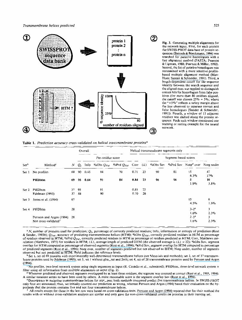
Fig. 3. Generating multiple alignments for the network input. First, for each protein the SWISS-PROT data base of protein se- quences (Bairoch & Boeckmann, 1994) was searched for putative homologues with a fast alignment method (FASTA; Pearson & Lipman, 1988; Pearson &Miller, 1992). Second, the list of putative homologues was reexamined with a more sensitive profile- based multiple alignment method (Max- Hom; Sander & Schneider, 1991). Third, a length-dependent cutoff for the sequence identity between the search sequence and the aligned ones was applied to distinguish correct hits for homologues from false pos- itives (for more than 80 residues aligned, the cutoff was chosen 25% + 5%; where the "+5%" reflects a safety margin above the line observed to separate correct and false homologues [Sander & Schneider, 19911). Fourth, a window of 13 adjacent residues was shifted along the protein se- quence. Each such window constituted one training or testing example for the neural

0 network

Table 1. Prediction accuracy cross-validated an helical transmembrane proteinsa "

.~

Overall Helical transmembrane segments only "_ ." "~

Per-residue score Segment-based scores _ _ _ ~

Set MethodC N Q2 Info %Obs QTM %Prd QTM Corr ( L ) %Obs Sov %Prd Sov Nsegd over Nseg under

Set 1 No profiles 69 90 0.45 84 70 0.71 23 90 81 15 47

PHDhlm 69 95 0.64 91 84 0.84 23 96 96 5 10 6.3% 17%

1.9% 3.8%

Set 2 PHDhtm 37 95 91 Edelman ( I 993) 37 88 90

Set 3 Jones et al. (1994) 67

Set 4 PHDhtm 28

Persson and Argos (1994) 28 Not cross-validatedf

0.85 23 0.70 26

I5 6 4.5% 1.9%

3-2' 3 1.6% 2.3% 2-3' 3 1.6% 2.3%

a N , number of proteins used for prediction; QI, percentage of correctly predicted residues; Info, information or entropy of prediction (Rost & Sander, 1993b); QTM, accuracy of predicting transmembrane helices (HTM); %Obs QTM, correctly predicted residues in HTM as percentage of residues observed in HTM; %Prd QTM, correctly predicted residues in HTM as percentage of residues predicted as HTM; Corr, Matthews cor- relation (Matthews, 1975) for residues in HTM; (L), average length of predicted HTM (the observed average is ( L ) = 22); %Obs Sov, segment overlap for HTM computed as percentage of observed segments (Rost et al., 1994); %Prd Sov, segment overlap for HTM computed as percentage of predicted segments (Rost et al., 1994); Nseg over, number of segments predicted but not observed as HTM; Nseg under, number of segments observed but not predicted as HTM. Bold indicates the reference levels.

Set 1, set of 69 proteins with experimentally well-determined transmembrane helices (see Materials and methods); set 2, set of 37 transmem- brane proteins used by Edelman (1993); set 3, set 1 without glra-rat and 2mlt; set 4, set of 28 transmembrane proteins used by Persson and Argos (1994).

No profiles, two-level network system using single sequences as input (R. Casadio et al., submitted); PHDhtm, three-level network system + filter using all information from multiple alignments as input (Fig. 2).

Whenever predicted and observed segments overlapped by at least three residues, the segment was counted as correct (Rost et al., 1993, 1994). A similar measure seems to have been used by others. A more reasonable score is the segment overlap Sov (Rost et al., 1994).

e Discrepancy in assigning transmembrane helices for atpi-pea; both methods compared predict five transmembrane helices. In SWISS-PROT only four are annotated; thus, we initially counted our prediction as wrong, whereas Persson and Argos (1994) based their evaluation on the hy- pothesis that the protein contains five and not four transmembrane helices.

All results except for those in the last row were based on cross-validation tests. Persson and Argos (1994) reported that for their method the results with or without cross-validation analysis are similar and only gave the non-cross-validated results on proteins in their training set.

526

A --e PHDhtm (input multiple alignment) ----x--- no profiles (input single sequences)

94- .............. + .............. i ............... i ............... i .............. I .............. 4

92 - .............. ;.. ............ i.. .............

90 I I 65 ?'O j 5 80 d5 $0 95 100

percentage of residues predicted

t5 B - compiled as percentage -o- % of predicted

+ 8 of observed

I I I I I

I I I I

. . ..........

: v . 90 .................... .................... ; .................... ....................

...................................................................................... * i .............. 3*y I I I I

0 20 40 60 80 1 0 0 percentage of residues predicted

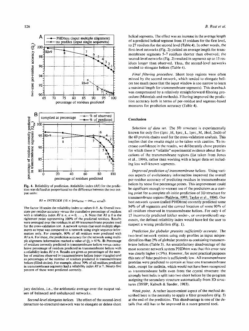
Fig. 4. Reliability of prediction. Reliability index ( R I ) for the predic- tion was defined as proportional to the difference between the two out- put units:

RI = INTEGER (10 X [OUtHTM - OUt,,,, HTM]) .

The factor 10 scales the reliability index to values 0-9. A: Overall two- state per-residue accuracy versus the cumulative percentage of residues with a reliability index RI 2 n, n = 0, . . . . 9. Note that RI 2 0 is the rightmost point representing 100% of the predicted residues. Results were averaged over the residues in all 69 transmembrane proteins used for the cross-validation test. A network system that used multiple align- ments as input was compared to a network using single sequence infor- mation only. For example, 90% of all residues were predicted with RI 2 6. For these, the prediction accuracy for the network using multi- ple alignment information reached a value of Q2 > 97%. B: Percentage of residues correctly predicted in transmembrane helices versus cumu- lative percentage of residues predicted in transmembrane helices with a reliability index RI 5 n. Results are given as percentages of the num- ber of residues observed in transmembrane helices (open triangles) and as percentages of the number of residues predicted in transmembrane helices (filled circles). For example, about 70% of all residues predicted in transmembrane segments had a reliability index RI 2 7. Ninety-five percent of these were predicted correctly.

jury decision, i.e., the arithmetic average over the output val- ues of balanced and unbalanced networks.

Second-level elongates helices. The effect of the second-level (structure-to-structure) network was to elongate or delete short

B. Rost et al.

helical segments. The effect was an increase in the average length of a predicted helical segment from 15 residues for the first level, to 27 residues for the second level (Table 4). In other words, the first-level networks (Fig. 2) yielded an average length for trans- membrane segments 5-7 residues shorter than observed; the second-level networks (Fig. 2) resulted in segments up to 13 res- idues longer than observed. Thus, the second-level networks tended to elongate helices (Table 4).

Final filtering procedure. Short loop regions were often missed by the second network, which tended to elongate heli- ces too much (note that the input window is too narrow to learn a maximal length for transmembrane segments). This drawback was compensated by a relatively straightforward filtering pro- cedure (Materials and methods). Filtering improved the predic- tion accuracy both in terms of per-residue and segment-based measures for prediction accuracy (Table 4).

Conclusion

Selection of data set. The 3D structure is experimentally known for only five (Iprc-H, lprc-L, Iprc-M, lbrd, 2mlt) of the 69 protein chains used for the cross-validation analysis. This implies that the results ought to be taken with caution. To in- crease confidence in the results, we deliberately chose proteins for which there is "reliable" experimental evidence about the lo- cations of the transmembrane regions (list taken from Jones et al., 1994), rather than working with a larger data set includ- ing less well-known segments.

Improvedprediction of transmembrane helices. Using vari- ous aspects of evolutionary information improved the overall per-residue accuracy of predicting residues in transmembrane helices by some five percentage points. This improvement could be significant enough to warrant use of the predictions as a start- ing point for a complete ab initio prediction of 3D structure for transmembrane regions (Baldwin, 1993; Taylor et al., 1994). Our best network system (called PHDhtm) correctly predicted some 94% of all segments and the correct location of some 90% of all residues observed in transmembrane helices. For only 4 of 15 incorrectly predicted (either under-, or overpredicted) seg- ments, the defined reliability index would have led the user to suspect a wrong prediction (Fig. 1).

Prediction for globular proteins sufficiently accurate. The two-level network system using only profiles as input mispre- dicted less than 2% of globular proteins as containing transmem- brane helices (Table 3). An unsatisfactory disadvantage of the most accurate network system PHDhtm was that this error rate was clearly higher (<5%) . However, for most practical purposes this rate of false positives is sufficiently low. All transmembrane proteins were predicted to contain at least one transmembrane helix, except for melittin, which would not have been recognized as transmembrane helix even from the crystal structure: the strongly bent helix is split into two short helices by the program assigning the secondary structure automatically from 3D struc- tures (DSSP; Kabsch & Sander, 1983).

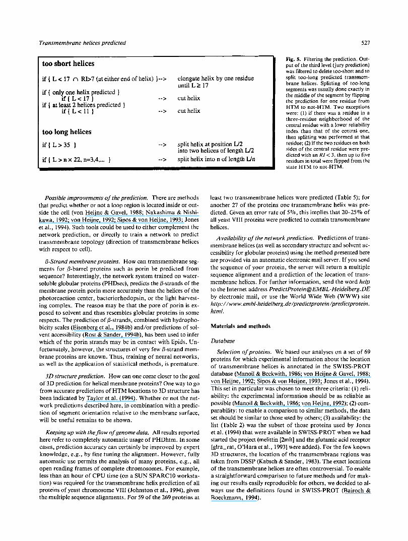
Weakpoint. A rather inconvenient aspect of the method de- scribed here is the necessity to apply a filter procedure (Fig. 5 ) at the end of the prediction. This disadvantage is one of the de- tails that still has to be improved in a more general tool.

Transmembrane helices predicted 527

too short helices

if ( L e 17 n R b 7 (at either end of helix) I--> elongate helix by one residue

if ( only one helix predicted )

if { at least 2 helices predicted }

until L 1 17

i f ( L < 1 7 ) --> cut helix

if ( L < 11 ) --> cut helix

too long helices

if ( L > 3 5 )

if { L > n x 22, n=3.4, ... }

--> split helix at position U2 into two helices of length U2

--> split helix into n of length U n

Fig. 5. Filtering the prediction. Out- put of the third level (jury prediction) was filtered to delete too-short and to split too-long predicted transmem- brane helices. Splitting of too-long segments was usually done exactly in the middle of the segment by flipping the prediction for one residue from HTM to not-HTM. Two exceptions were: ( I ) if there was a residue in a three-residue neighborhood of the central residue with a lower reliability index than that of the central one, then splitting was performed at that residue; (2) if the two residues on both sides of the central residue were pre- dicted with an RI < 3, then up to five residues in total were flipped from the state HTM to not-HTM.

Possible improvements of the prediction. There are methods that predict whether or not a loop region is located inside or out- side the cell (von Heijne & Gavel, 1988; Nakashima & Nishi- kawa, 1992; von Heijne, 1992; Sipos & von Heijne, 1993; Jones et al., 1994). Such tools could be used to either complement the network prediction, or directly to train a network to predict transmembrane topology (direction of transmembrane helices with respect to cell).

@-Strand membrane proteins. How can transmembrane seg- ments for @-barrel proteins such as porin be predicted from sequence? Interestingly, the network system trained on water- soluble globular proteins (PHDsec), predicts the @-strands of the membrane protein porin more accurately than the helices of the photoreaction center, bacteriorhodopsin, or the light harvest- ing complex. The reason may be that the pore of porin is ex- posed to solvent and thus resembles globular proteins in some respects. The prediction of @-strands, combined with hydropho- bicity scales (Eisenberg et al., 1984b) and/or predictions of sol- vent accessibility (Rost & Sander, 1994b), has been used to infer which of the porin strands may be in contact with lipids. Un- fortunately, however, the structures of very few @-strand mem- brane proteins are known. Thus, training of neural networks, as well as the application of statistical methods, is premature.

3 0 structure prediction. How can one come closer to the goal of 3D prediction for helical membrane proteins? One way to go from accurate predictions of HTM locations to 3D structure has been indicated by Taylor et al. (1994). Whether or not the net- work predictions described here, in combination with a predic- tion of segment orientation relative to the membrane surface, will be useful remains to be shown.

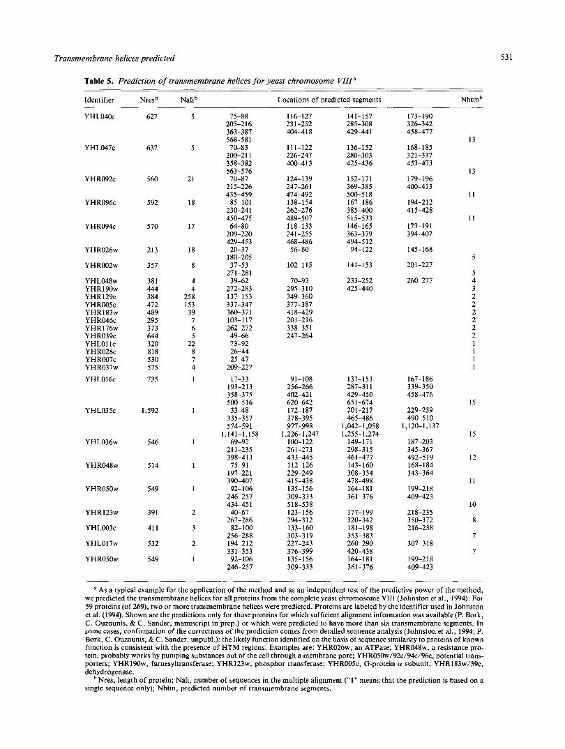
Keeping up with thejlow of genome data. All results reported here refer to completely automatic usage of PHDhtm. In some cases, prediction accuracy can certainly be improved by expert knowledge, e.g., by fine tuning the alignment. However, fully automatic use permits the analysis of many proteins, e.g., all open reading frames of complete chromosomes. For example, less than an hour of CPU time (on a SUN SPARClO worksta- tion) was required for the transmembrane helix prediction of all proteins of yeast chromosome VI11 (Johnston et al., 1994), given the multiple sequence alignments. For 59 of the 269 proteins at

least two transmembrane helices were predicted (Table 5 ) ; for another 27 of the proteins one transmembrane helix was pre- dicted. Given an error rate of 570, this implies that 20-2570 of all yeast VI11 proteins were predicted to contain transmembrane helices.

Availability of the network prediction. Predictions of trans- membrane helices (as well as secondary structure and solvent ac- cessibility for globular proteins) using the method presented here are provided via an automatic electronic mail server. If you send the sequence of your protein, the server will return a multiple sequence alignment and a prediction of the location of trans- membrane helices. For further information, send the word help to the Internet address [email protected] by electronic mail, or use the World Wide Web (WWW) site http://www.embl-heidelberg.de/predictprotein/predictprotein. html.

Materials and methods

Database

Selection of proteins. We based our analyses on a set of 69 proteins for which experimental information about the location of transmembrane helices is annotated in the SWISS-PROT database (Manoil & Beckwith, 1986; von Heijne & Gavel, 1988; von Heijne, 1992; Sipos & von Heijne, 1993; Jones et al., 1994). This set in particular was chosen to meet three criteria: (1) reli- ability: the experimental information should be as reliable as possible (Manoil & Beckwith, 1986; von Heijne, 1992); (2) com- parability: to enable a comparison to similar methods, the data set should be similar to those used by others; (3) availability: the list (Table 2) was the subset of those proteins used by Jones et al. (1994) that were available in SWISS-PROT when we had started the project (melittin [2mlt] and the glutamic acid receptor [glra-rat, O’Hara et al., 19931 were added). For the few known 3D structures, the location of the transmembrane regions was taken from DSSP (Kabsch & Sander, 1983). The exact locations of the transmembrane helices are often controversial. To enable a straightforward comparison to future methods and for mak- ing our results easily reproducible for others, we decided to al- ways use the definitions found in SWISS-PROT (Bairoch & Boeckmann, 1994).

528

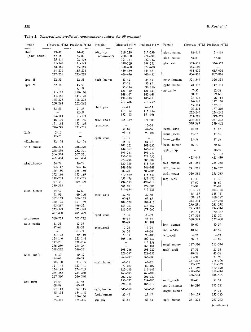
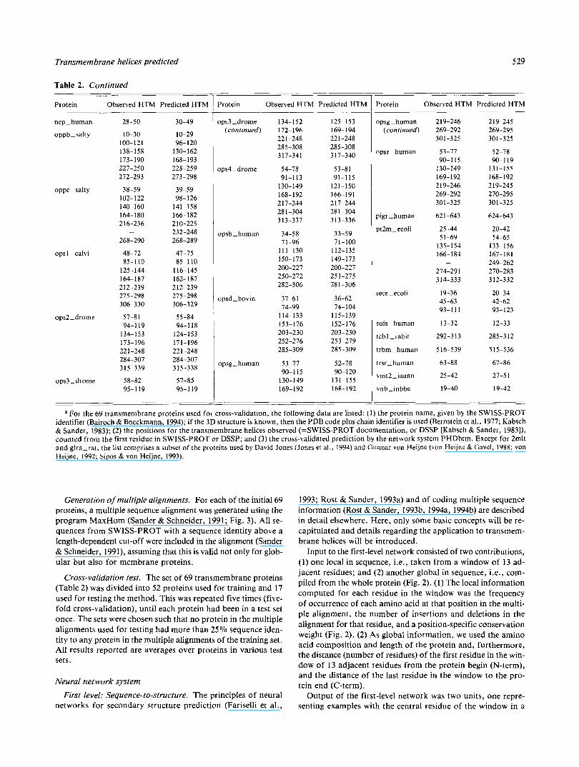
Table 2. Observed and predicted transmembrane helices for 69 proteinsa

Protein Observed HTM Predicted HTM .- c

1 brd (bacr-halha)

lprc-H

lprc-M

I prc- L

2mlt

4f2-human

5ht3Lmouse

alaa-human

a4Lhuman

aalr-canfa

adt-ricpr

23-42 57-76 95-1 14

121-140 148-167 191-210 217-236

12-35

52-76

11 1-137 143-166 198-223 260-284

33-53

84-1 I 1 116-139 171-198 226-249

2-10 12-25

82-104

246-272 278-296 306-324 465-484

54-79 92-117

128-150 172- 196

-

-

210-233 307-33 1 339-363

34-59 71-96

107-129 150- 173 193-217 375-399 407-430

700-723

11-33 47-69

81-102 -

124- 146 177-201 236-259 268-292

8-30 44-66 78-100

121-143 174-198

267-290

34-54 68-88 93-113

148-168

185-205

235-258

-

24-43 55-87 92-116

121-143 145-169 185-21 1 213-239

12-3 I

43-59 63-78

110-130 143-170 198-223 262-292

21-38 42-58 81-103

115-146 173-196 223-255

-

-

82-104

238-270 282-301 307-33 1 457-484

56-79 92-116

128-150 173-189 213-235 309-329

-

32-60 69- 100

106-133 151-169 196-221 375-399 405-429

702-722

12-35 39-53 61-74 80- 1 10

125-144 176-206 235-261 266-291

10-32 40-7 1 77-105

122-141 174-203 234-260 266-290

3 1-46 60-87 92-115

134-148 156-170 185-206

~-

Protein Observed HTM Predicted HTM ~~

adt-ricpr (continued)

bach-halhm

cb2lLpea

cek2-chick

cyoa-ecoli

:yob-ecoli

:yoc-ecoli

:yodLecoli

:yoe-ecoli

Zdgl-human

egfr-human

fce2Lhuman

glp-pig

~"

2 19-239 280-300 321-341 349-369 380-400 439-459 466-486

23-42

95-1 14 121-140 148-167 191-210

57-76

217-236

62-8 1 114-134 182- 198

365-389

5 1-69 93-1 11

-

17-35 58-76

102-121 144-162 195-213 232-250 277-296 320-339 348-366 382-401 4 10-429 457-476 494-5 13 588-607 6 14-634

32-50 67-85

102-120 143-161 185-203

18-36 46-64 81-99

10-28 38-56 79-97

108-126 - -

198-216 229-247 269-287

47-71 79-107

122-140 160-185 202-222 256-277 294-3 14

646-668

22-47

63-85

~"

217-239 27 1-298 322-342 348-371 377-400 444-461 469-485

24-43 55-87 92-1 I6

121-143 145-169 185-211 213-239

69-75 115-134 184-196

371-389

12-24 44-66 90- 109

61-77 101-131 146-158 191-212 227-252 286-302 315-335 349-368 380-401 415-440 457-470 498-519 592-608 6 12-626

29-50 67-85

101-116 138-162 178-202

20-39 45-64 80-101

12-24 44-66 90- 109

109-127 142-158 166-181 198-222 228-252 265-287

45-72 80- 107

116-145 160-180 201-227 254-282 288-3 12

648-666

27-47

63-84

-

B. Rost et al.

- ~. ~ ~~~

Protein Observed HTM Predicted HTM ~

glpa-human

glpc-human

glra-rat

gmcr-human

gplb-human

gpt-crilo

hema-cdvo

hema-measi

h e m a ~ p i 4 h a

hg2achuman

iggb-strsp

il2a-human

il2b-human

ita5Lmouse

lacy-ecoli

lech-human

leci-mouse

lep-ecoli

magl-mouse

malf-ecoli

motb-ecoli

mprd-human

mypO-human

ngfr-human

92-1 14

58-81

539-558 585-603 614-632 806-826

321-346

148-172

7-32 58-79 95-1 14

126-145 165-184 195-211 222-240 253-269 275-294 379-397

35-55

35-55

35-59

46-72 -

-

423-443

241-259

241-265

356-381

11-33 47-67 75-99

103-125 145-163 168-187 2 12-234 260-281 291-310 315-334 347-366 380-399

40-60

40-60

4-22 58-76

517-536

17-35 40-58 73-91

277-295 319-337 371-389 418-436 486-504

28-49

186-210 -

154-179

25 1-272

~~~

91-1 14

57-81

536-557

615-636 807-826

326-35 1

147-171

12-38 59-83 96-115

127-150 157-181 187-210 224-242 249-269 277-292 379-402

37-58

37-58

37-59

50-67

18-32 91-103

425-439

235-258

236-267

-

355-383

11-36 46-67 75-98

104- 126 148-161 169-187 219-238 265-288 294-314 320-337 343-371 377-400

40-59

40-59

4-23 63-82

515-534

21-35 43-58 7 1-93

278-306 318-339 370-390 418-444 486-505

30-5 1

185-21 1

14-3 I 155-183

253-272

(continued)

Transmembrane helices predicted 529

Table 2. Continued

Protein Observed HTM Predicted HTM

nep-human

oppb-salty

oppc-salty

opsl -calvi

ops2-drome

OpS3-drome

28-50

10-30 100-121 138-158 173-190 227-250 272-293

38-59 102-122 140-160 164- 180 216-236

268-290

48-72 85-1 10

125-144 164- 187 212-239 275-298 306-330

-

57-81 94-1 I9

134-153 173-196 221-248 284-307 315-339

58-82 95-1 I9

30-49

10-29 96- 120

130- 162 168-193 228-259 273-298

39-59 98-126

141-158 166- 182 2 10-22s 232-248 268-289

47-75 85-1 10

116-145

212-239 275-298

162- 187

306-329

55-84 94-118

124-153 171-196 221 -248 284-307 315-338

57-85 95-119

Protein Observed HTM Predicted HTM

ops3-drome (conrinued)

ops4-drome

opsb-human

opsd-bovin

opsg-human

134-152 172- I96 22 1-248 285-308 317-341

54-78 91-113

130-149 168- 192 217-244 28 1-304 313-337

34-58 7 1-96

111-130 150- 173 200-227 250-272 282-306

37-61 74-99

114-133 153-176 203-230 252-276 285-309

53-77 90-115

130-149 169-192

125-153 169-194 22 1-248 285-308 3 17-340

53-81 91-115

121-150 166-191 2 17-244 28 1-304 3 13-336

33-59 71-100

112-135 149-173 200-227 251-275 281-306

36-62 74- 104

115-139 152-176 203-230 253-279 285-309

52-78 90- 1 20

131-155 168-192

Protein Observed HTM Predicted HTM

opsg-human (continued)

opsr-human

pigr-human

pt2m-ecoli

sece-ecoli

suis-human

tcbl -rabit

trbm-human

trsr-human

vmt2Liaann

vnb-inbbe

"

2 19-246 269-292 301-325

53-77 90-1 I5

130-149 169-192 2 19-246 269-292 301-325

62 1-643

25-44 5 1-69

135-154 166- 184

274-291 -

314-333

19-36 45-63 93-1 1 1

13-32

292-3 I3

5 16-539

63-88

25-42

19-40

2 19-245 269-295 301-325

52-78 90-1 I9

131-155 168- 192 219-245 270-295 301-325

624-643

20-42 54-65

133-156 167-181 249-262 270-283 312-332

20-34 42-62 93-123

12-33

285-312

5 15-536

67-86

27-5 1

19-42

_" a For the 69 transmembrane proteins used for cross-validation, the following data are listed: (1) the protein name, given by the SWISS-PROT

identifier (Bairoch & Boeckmann, 1994); if the 3D structure is known, then the PDB code plus chain identifier is used (Bernstein et ai., 1977; Kabsch & Sander, 1983); (2) the positions for the transmembrane helices observed (=SWISS-PROT documentation, or DSSP [Kabsch & Sander, 1983]), counted from the first residue in SWISS-PROT or DSSP; and (3) the cross-validated prediction by the network system PHDhtm. Except for 2mlt and glra-rat. the list comprises a subset of the proteins used by David Jones (Jones et al., 1994) and Gunnar von Heijne (von Heijne & Gavel, 1988; von Heijne, 1992; Sipos & von Heijne, 1993).

Generation of multiple alignments. For each of the initial 69 proteins, a multiple sequence alignment was generated using the program MaxHom (Sander & Schneider, 1991; Fig. 3). All se- quences from SWISS-PROT with a sequence identity above a length-dependent cut-off were included in the alignment (Sander & Schneider, 1991), assuming that this is valid not only for glob- ular but also for membrane proteins.

Cross-validation test. The set of 69 transmembrane proteins (Table 2) was divided into 52 proteins used for training and 17 used for testing the method. This was repeated five times (five- fold cross-validation), until each protein had been in a test set once. The sets were chosen such that no protein in the multiple alignments used for testing had more than 25% sequence iden- tity to any protein in the multiple alignments of the training set. All results reported are averages over proteins in various test sets.

Neural network system First level: Sequence-to-structure. The principles of neural

networks for secondary structure prediction (Fariselli et al.,

1993; Rost & Sander, 1993a) and of coding multiple sequence information (Rost & Sander, 1993b, 1994a, 1994b) are described in detail elsewhere. Here, only some basic concepts will be re- capitulated and details regarding the application to transmem- brane helices will be introduced.

Input to the first-level network consisted of two contributions, (1) one local in sequence, Le., taken from a window of 13 ad- jacent residues; and (2) another global in sequence, i.e., com- piled from the whole protein (Fig. 2 ) . (1) The local information computed for each residue in the window was the frequency of occurrence of each amino acid at that position in the multi- ple alignment, the number of insertions and deletions in the alignment for that residue, and a position-specific conservation weight (Fig. 2) . ( 2 ) As global information, we used the amino acid composition and length of the protein and, furthermore, the distance (number of residues) of the first residue in the win- dow of 13 adjacent residues from the protein begin (N-term), and the distance of the last residue in the window to the pro- tein end (C-term).

Output of the first-level network was two units, one repre- senting examples with the central residue of the window in a

530 B. Rost et al.

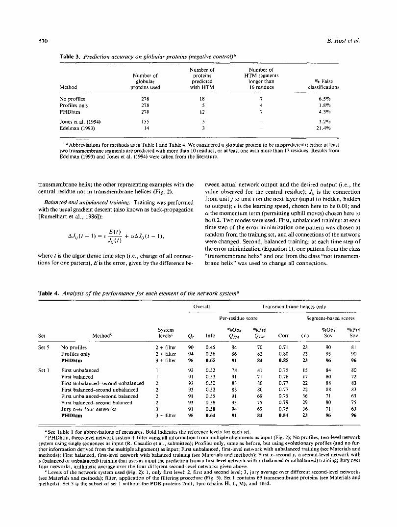
Table 3. Prediction accuracy on globular proteins (negative control) a

Method

Number of Number of Number of proteins HTM segments

globular predicted longer than % False proteins used with HTM 16 residues classifications

No profiles Profiles only PHDhtm

278 278 278

Jones et al. (1994) 155 Edelman (1993) 14

18 5

12

5 3

6.5% 1.8% 4.3%

3.2% 21.4%

a Abbreviations for methods as in Table 1 and Table 4. We considered a globular protein to be mispredicted if either at least two transmembrane segments are predicted with more than 10 residues, or at least one with more than 17 residues. Results from Edelman (1993) and Jones et al. (1994) were taken from the literature.

transmembrane helix; the other representing examples with the central residue not in transmembrane helices (Fig. 2 ) .

Balanced and unbalanced training. Training was performed with the usual gradient descent (also known as back-propagation [Rumelhart et al., 19861):

where tis the algorithmic time step (i.e., change of all connec- tions for one pattern), E is the error, given by the difference be-

tween actual network output and the desired output (i.e., the value observed for the central residue); J j is the connection from unit j to unit i on the next layer (input to hidden, hidden to output); E is the learning speed, chosen here to be 0.01; and CY the momentum term (permitting uphill moves) chosen here to be 0.2. Two modes were used. First, unbalanced training: at each time step of the error minimization one pattern was chosen at random from the training set, and all connections of the network were changed. Second, balanced training: at each time step of the error minimization (Equation l) , one pattern from the class “transmembrane helix” and one from the class “not transmem- brane helix” was used to change all connections.

Table 4. Analysis of the performance for each element of the network systema

Overall ~ ~

System ”

Set Methodb levels‘ Q2

Set 5 No profiles 2 + filter 90 Profiles only 2 + filter 94 PHDhtm 3 + filter 95

Set 1 First unbalanced 1 93 First balanced 1 91 First unbalanced-second unbalanced 2 93 First balanced-second unbalanced 2 93 First unbalanced-second balanced 2 91 First balanced-second balanced 2 93 Jury over four networks 3 91 PHDhtm 3 + filter 95

~

Info

0.45 0.56 0.65

0.52 0.53 0.52 0.52 0.55 0.58 0.58 0.64

Transmembrane helices only ””

Per-residue score Segment-based scores ~~

%Obs %Prd %Obs %Prd QTM QTM Corr ( L ) Sov sov

84 70 0.71 23 90 81 86 82 0.80 23 93 90 91 84 0.85 23 96 96

78 81 0.75 15 84 80 91 71 0.76 17 80 72 83 80 0.77 22 88 83 83 80 0.77 22 88 83 91 69 0.75 36 71 63 93 75 0.79 29 80 75 94 69 0.75 36 71 63 91 84 0.84 23 96 96

.”~.

a See Table 1 for abbreviations of measures. Bold indicates the reference levels for each set. PHDhtm, three-level network system + filter using all information from multiple alignments as input (Fig. 2); No profiles, two-level network

system using single sequences as input (R. Casadio et al., submitted); Profiles only, same as before, but using evolutionary profiles (and no fur- ther information derived from the multiple alignment) as input; First unbalanced, first-level network with unbalanced training (see Materials and methods); First balanced, first-level network with balanced training (see Materials and methods); First x-second JJ, a second-level network with JJ (balanced or unbalanced) training that uses as input the prediction from a first-level network with x (balanced or unbalanced) training; Jury over four networks, arithmetic average over the four different second-level networks given above.

Levels of the network system used (Fig. 2): 1, only first level; 2, first and second level; 3, jury average over different second-level networks (see Materials and methods); filter, application of the filtering procedure (Fig. 5) . Set 1 contains 69 transmembrane proteins (see Materials and methods). Set 5 is the subset of set 1 without the PDB proteins 2mlt, lprc (chains H, L, M), and lbrd.

Transmembrane helices predicted 531

Table 5. Prediction of transmembrane helices for yeast chromosome VUIa

Identifier Nresb Nalib

YHL040c

YHL047c

YHR092c

YHR096c

YHR094c

YHR026w

YHR002w

YHL048w YHR190w YHR129c YHR005c YHR183w YHR046c YHR176w YHR039c YHLOl I C YHR028c YHR007c YHR037w

YHL016c

YHL035c

YHL036w

YHR048w

YHRO5Ow

YHR123w

YHL003c

YHL017w

YHRO5Ow

627

637

5 60

592

570

213

357

381 444 3 84 472 489 295 373 644 320 818 530 575

735

1,592

546

514

549

391

41 1

532

549

-~ -~

5

5

21

18

17

18

8

4 4

258 153 39 7 6

22 5

8 7 4 1

1

1

1

1

2

3

2

1

205-216 75-88

363-387 568-581

200-21 1 70-83

358-382 563-576

215-226 70-87

435-459 85-101

230-241 450-475 64-80

209-220 429-453 20-37

180-205 37-53

271-281 39-62

272-283 137-153 337-347 360-371 103-117 262-272 49-66 13-92 26-44 25-47

209-227 17-33

358-375 193-213

500-516

335-357 33-48

574-591 1,141-1.158

69-92 21 1-235 398-413 75-91

197-221 390-407 92- 106

246-257 434-45 1

267-286 40-67

82-100 256-288 194-212 331-353 92-106

246-257

Locations of predicted segments

231-252 404-4 1 8

111-122 226-247 400-41 3

116-127

124-139 247-261 474-492 138-154 262-276 489-507 118-133 241-255 468-486

56-80

102-115

70-93 295-310 349-360 377-387 41 8-429 201-216 338-351 247-264

91-108

402-421 256-266

172-187

977-998 1,226-1,247

100-122 261-273 433-445

229-249 112-126

415-438

620-642

378-395

309-333 135-156

518-538 123-156 294-3 12 133-160 303-3 19 227-243

135-156 376-399

309-333

285-308 429-441

141-157

136-152 280-303 425-436

369-385 152-171

500-5 18 167- 186 385-400 515-533 146-165 363-379 494-512 94- 122

141-153

233-252 425-440

137-153 287-3 1 I 429-450 65 1-674 201-217 465-486

1,042-1,058 1 1.255-1.274

298-3 15 149-171

461-477 143-160 308-334 478-498

361-376 164-181

177- 199 320-342 181-198 353-383 260-290 420-438 164-181 361-376

326-342 173-190

458-477

168-185 321-337 453-473

179-196 400-41 3

194-212 415-428

173-191 394-407

145- 168

201-227

260-277

167-186 339-350 458-476

229-239 490-5 10

,120-1,137

187-203 345-367 492-5 19 168-184 343-364

199-21 8 409-423

218-235 350-372 216-238

307-3 18

199-218 409-423

Nhtmb ~

13

13

11

11

5

5 4 3 2 2 2 2 2 2 1 1 1 1

15

15

12

11

10

8

7

7

a As a typical example for the application of the method and as an independent test of the predictive power of the method, we predicted the transmembrane helices for all proteins from the complete yeast chromosome VI11 (Johnston et al., 1994). For 59 proteins (of 269). two or more transmembrane helices were predicted. Proteins are labeled by the identifier used in Johnston et al. (1994). Shown are the predictions only for those proteins for which sufficient alignment information was available (P. Bork, C. Ouzounis, & C. Sander, manuscript in prep.) or which were predicted to have more than six transmembrane segments. In some cases, confirmation of the correctness of the prediction comes from detailed sequence analysis (Johnston et al., 1994; P. Bork, C. Ouzounis, & C. Sander, unpubl.): the likely function identified on the basis of sequence similarity to proteins of known function is consistent with the presence of HTM regions. Examples are: YHR026w, an ATPase; YHR048w. a resistance pro- tein, probably works by pumping substances out of the cell through a membrane pore; YHR050~/92~/94~/96c, potential trans- porters; YHR190w, farnesyltransferase; YHR123w, phosphor transferase; YHROOSc, G-protein a subunit; YHR183w/39c, dehydrogenase.

Nres, length of protein; Nali, number of sequences in the multiple alignment (“1” means that the prediction is based on a single sequence only); Nhtm, predicted number of transmembrane segments.

532 B. Rost et al.

Networkparameters. All units were connected to all those on the next layer (input to hidden, hidden to output). Network pa- rameters such as criterion to terminate the training procedure, number of hidden units, training speed ( e in Equation l), and momentum term (a in Equation 1) were chosen arbitrarily based on our experience with secondary structure prediction for glob- ular proteins. In other words, these parameters were not influ- enced by the test set. Training was stopped when the training set had been learned to an accuracy of 93% for the first- and of 95% for the second-level network. As for the number of hid- den units, we started arbitrarily with 3 hidden units for the first level of network and increased the number for the second-level network to 15 because training too often ended in local minima.

Second level: Structure to structure. The input to the second- level network consisted - as for the first-level - of a contribu- tion local in sequence and a contribution global in sequence (Fig. 2). (1) For each residue in the input window, the local input were the values of the two output units of the first-level network and the conservation weight. (2) The global input in- formation was the same as for the first-level network. The out- put of the second-level network - as for the first - consisted of two units for the central residue either being in a transmembrane helix or not.

Third level: Jury decision. To find a compromise between networks with balanced and those with unbalanced training, a final jury decision was performed (effectively a compromise between over- and underprediction, Results). The jury decision was a simple arithmetic average over four differently trained networks: all combinations (2 x 2) of first-level network with balanced and unbalanced training, and with balanced or unbal- anced training of second-level network. Final prediction was as- signed to the unit with maximal output value (“winner takes all”).

Fourth level: Filtering the prediction. In contrast to earlier prediction methods (Jones et al., 1992; von Heijne, 1992; Pers- son & Argos, 1994), which explicitly fix the length of predicted transmembrane segments to typically 17-25 residues, the second- level network occasionally resulted in transmembrane helices that were either too short or too long. This was corrected by a nonoptimized filter that was guided by the experiences of pre- vious work (von Heijne, 1986, 1992; von Heijne & Gavel, 1988; Sipos & von Heijne, 1993; Jones et al., 1994; R. Casadio et al., submitted).

Too long helices were either split in the middle into two shorter helices or were shortened (Fig. 5 ) . Too short helices were either elongated or deleted. All these decisions (split or shorten; elongate or delete) were based both on the strength of the pre- diction (reliability index, Fig. 2) and on the length of the pre- dicted transmembrane helix (Fig. 5 ) .

Acknowledgments

We are grateful to Reinhard Schneider (EMBL, Heidelberg) for provid- ing the latest version of the alignment program MaxHom; Chiara Taroni (Bologna) and Mario Compiani (Camerino) for helpful discussions; Da- vid Jones (London) for help with the data set; Gunnar von Heijne (Hud- dinge) for motivating discussions; and Christos Ouzounis (EMBL) for providing the multiple alignments for yeast VIII. We thank the two ref- erees, who helped improve the text by their detailed criticism. Last, but not least, we thank all those who deposit experimental results in public databases.

References

Argos P, Rao JKM, Hargrave PA. 1982. Structural prediction of membrane- bound proteins. Eur J Eiochem 128565-575.

Bairoch A, Boeckmann B. 1994. The SWISS-PROT protein sequence data bank: Current status. Nucleic Acids Res 22:3578-3580.

Baldwin JM. 1993. The probable arrangement of the helices in G protein- coupled receptors. EMEO J 12:1693-1703.

Bernstein FC, Koetzle TF, Williams GJB, Meyer EF Jr , Brice MD, Rodgers JR, Kennard 0, Shimanouchi T, Tasumi M. 1977. The Protein Data

Mol Eiol 112:535-542. Bank: A computer based archival file for macromolecular structures. J

Cornette JL, Cease KB, Margalit H, Spouge JL, Berzofsky JA, DeLisi C. 1987. Hydrophobicity scales and computational techniques for detect- ing amphipathic structures in proteins. J Mol Eiol 195:659-685.

Cowan SW, Rosenbusch JP. 1994. Folding pattern diversity of integral mem- brane proteins. Science 264:914-916.

Degli Esposti M, Crimi M, Venturoli G. 1990. A critical evaluation of the

Deisenhofer J, Epp 0, Mii K, Huber R, Michel H. 1985. Structure of the hydropathy profile of membrane proteins. Eur JEiochem 190:207-219.

protein subunits ia the photosynthetic reaction centre of Rhodopseudom- onas viridis at 3 A resolution. Naiure 318:618-624.

Edelman J. 1993. Quadratic minimization of predictors for protein second- ary structure: Application to transmembrane a-helices. JMol Eiol232: 165-191.

Eisenberg D, Schwartz E, Komaromy M, Wall R. 1984a. Analysis of mem-

J Mol Biol 179:125-142. brane and surface protein sequences with the hydrophobic moment plot.

Eisenberg D, Weiss RM, Terwilliger TC. 1984b. The hydrophobic moment detects periodicity in protein hydrophobicity. Proc Nail Acad Sci USA 81:140-144.

Engelman DM, Steitz TA, Goldman A. 1986. Identifying nonpolar trans- bilayer helices in amino acid sequences of membrane proteins. Annu Rev Eiophys Eiophys Chem 15:321-353.

Fariselli P, Compiani M, Casadio R. 1993. Predicting secondary structures of membrane proteins with neural networks. Eur Eiophys J22:41-51.

Henderson R, Baldwin JM, Ceska TA, Zemlin F, Beckmann E, Downing KH. 1990. Model for the structure of bacteriorhodopsin based on high- resolution electron cryo-microscopy. J Mol Eiol 213399-929.

Johnston M, et al. [35 authors]. 1994. Complete nucleotide sequence of Sac- charomyces cerevisiae chromosome VIII. Science 265:2077-2082.

Jones DT, Taylor WR, Thornton JM. 1992. The rapid generation of muta-

Jones DT, Taylor WR, Thornton JM. 1994. A model recognition approach tion data matrices from protein sequences. CAEIOS 8:275-282.

to the prediction of all-helical membrane protein structure and topology. Biochemistry 33:3038-3049.

Kabsch W, Sander C. 1983. Dictionary of protein secondary structure: Pat- tern recognition of hydrogen bonded and geometrical features. Eiopoly- mers 22:2577-2637.

Kuhlbrandt W, Wang DN, Fujiyoshi Y. 1994. Atomic model of plant light-

Kyte J , Doolittle RF. 1982. A simple method for displaying the hydropathic harvesting complex by electron crystallography. Nature 367:614-621.

Landolt-Marticorena C, Williams KA, Deber CM, Reithmeier RAF. 1992. character of a protein. J Mol Eiol157:105-132.

of human type 1 single span membrane proteins. JMol Eiol229:602-608. Non-random distribution of amino acids in the transmembrane segments

Lattman EE. 1994. Protein crystallography for all. Proieins Struct Funci Genet 18:103-106.

Manoil C, Beckwith J. 1986. A genetic approach to analyzing membrane pro- tein topology. Science 233:1403-1408.

Matthews BW. 1975. Comparison of the predicted and observed secondary structure of T4 phage lysozyme. Eiochim Eiophys Acta 405:442-451.

Nakashima H, Nishikawa K. 1992. The amino acid composition is differ- ent between the cytoplasmic and extracellular sides in membrane pro-

O’Hara PJ, Sheppard PO, Thbgersen H, Venezia D, Haldeman BA, teins. FEES Left 303:141-146.

McGrane V, Houamed KM, Thomsen C, Gilbert TL, Mulvihill ER. 1993. The ligand-binding domain in metabotropic glutamate receptors is re-

Oliver s, et al. [152 authors]. 1992. The complete DNA sequence of yeast lated to bacterial periplasmic binding proteins. Neuron 11:41-52.

chromosome 111. Nature 357:38-46. Pearson WR, Lipman DJ. 1988. Improved tools for biological sequence com-

parison. Proc Nail Acad Sci USA 85:2444-2448. Pearson WR, Miller W. 1992. Dynamic programming algorithms for bio-

logical sequence comparison. Methods Enzymol210:575-601. Persson B, Argos P. 1994. Prediction of transmembrane segments in pro-

teins utilising multiple sequence alignments. J Mol Eiol 237:182-192. Rost B, Sander C. 1993a. Improved prediction of protein secondary struc-

Transmembrane helices predicted 533

ture by use of sequence profiles and neural networks. Proc Nut1 Acud Sci USA 90:7558-7562.

Rost B, Sander C. 1993b. Prediction of protein secondary structure at bet- ter than 70% accuracy. JMol Biol232:584-599.

Rost B, Sander C. 1993c. Secondary structure prediction of all-helical pro- teins in two states. Protein Eng 62331-836.

Rost B, Sander C. 1994a. Combining evolutionary information and neural networks to predict protein secondary structure. Proteins Struct Funct Genet 19:55-72.

Rost B, Sander C. 1994b. Conservation and prediction of solvent accessi- bility in protein families. Proteins Struct Funct Genet 20:216-226.

Rost B, Sander C, Schneider R. 1993. Progress in protein structure predic- tion? Trends Biochem Sci 18:120-123.

Rost B, Sander C, Schneider R. 1994. Redefining the goals of protein sec- ondary structure prediction. JMol Biol235:13-26.

Rumelhart DE, Hinton GE, Williams RJ. 1986. Learning representations by back-propagating error. Nature 323:533-536.

Sander C, Schneider R. 1991. Database of homology-derived structures and the structural meaning of sequence alignment. Proteins Struct Funct Ge- net 9:56-68.

Sander C, Schneider R. 1994. The HSSP database of protein structure- sequence alignments. Nucleic Acids Res 22:3597-3599.

Sipos L, von Heijne G. 1993. Predicting the topology of eukaryotic mem- brane proteins. Eur J Biochem 213:1333-1340.

Taylor WR, Jones DT, Green NM. 1994. A method for cy-helical integral membrane protein fold prediction. Proteins Struct Funct Genet 18:

von Heijne G. 1981. Membrane proteins-The amino acid composition of membrane-penetrating segments. Eur J Biochem 120:275-278.

von Heijne G. 1986. A new method for predicting signal sequence cleavage sites. Nucleic Acids Res 14:4683-4690.

von Heijne G. 1991. Computer analysis of DNA and protein sequences. Eur J Biochem 199:253-256.

von Heijne G. 1992. Membrane protein structure prediction. J Mol Biol 225:487-494.

von Heijne G, Gavel Y. 1988. Topogenic signals in integral membrane pro- teins. Eur J Biochem 174:671-678.

Wang DN, Kiihlbrandt W, Sarabiah V, Reithmeier RAF. 1993. Two- dimensional structure of the membrane domain of human Band 3 , the anion transport protein of erythrocyte membrane. EMBO J 12:2233- 2239.

Weiss MS, Schulz GE. 1992. Structure of porin refined at 1.8 A resolution. J Mol Biol227:493-509.

281-294.