Translation position determination in ptychographic coherent diffraction imaging

$Page 1: Translation position determination in ptychographic coherent diffraction imaging$
Translation position determination in

ptychographic coherent diffraction imaging

Fucai Zhang,1,2,3,*

Isaac Peterson,1,4,9

Joan Vila-Comamala,5,6

Ana Diaz,5 Felisa

Berenguer,1,7

Richard Bean,1,8

Bo Chen,1,3

Andreas Menzel,5 Ian K. Robinson,

1,3 and

John M. Rodenburg2,3

1 London Centre for Nanotechnology, UCL, London, WC1H 0AH, UK

2Department of Electronic & Electrical Engineering, University of Sheffield S1 3JD, UK 3 Research Complex at Harwell, Harwell Oxford, OX11 0FA, UK

4 School of Physics, University of Melbourne, Victoria 3010, Australia 5 Paul Scherrer Institut, 5232 Villigen PSI, Switzerland

6 Current address: Diamond Light Source Ltd, Harwell, OX11 0DE, UK 7 Current address: Synchrotron Soleil, L’Orme des Merisiers, Saint-Aubin, 94192 Gif-sur-Yvette, France

8 Current address: Center for Free-Electron Laser Science, Notkestr. 85, 22607 Hamburg, Germany 9Australian Research Council, Centre of Excellence for Coherent X-Ray Science, Australia

* [email protected]

Abstract: Accurate knowledge of translation positions is essential in

ptychography to achieve a good image quality and the diffraction limited

resolution. We propose a method to retrieve and correct position errors

during the image reconstruction iterations. Sub-pixel position accuracy after

refinement is shown to be achievable within several tens of iterations.

Simulation and experimental results for both optical and X-ray wavelengths

are given. The method improves both the quality of the retrieved object

image and relaxes the position accuracy requirement while acquiring the

diffraction patterns.

©2013 Optical Society of America

OCIS codes: (100.5070) Phase retrieval; (170.3010) Image reconstruction techniques;

(340.7440) X-ray imaging.

References and links

1. H. M. L. Faulkner and J. M. Rodenburg, “Movable aperture lensless transmission microscope: a novel phase

retrieval algorithm,” Phys. Rev. Lett. 93, 023903 (2004). 2. J. M. Rodenburg and H. M. L. Faulkner, “A phase retrieval algorithm for shifting illumination,” Appl. Phys.

Lett. 85(20), 4795–4797 (2004).

3. J. M. Rodenburg, “Ptychography and related diffractive imaging methods,” Adv. Imag. Elec. Phys. 150, 87–184 (2008).

4. J. M. Rodenburg, A. C. Hurst, A. G. Cullis, B. R. Dobson, F. Pfeiffer, O. Bunk, C. David, K. Jefimovs, and I.

Johnson, “Hard X-ray lensless imaging of extended objects,” Phys. Rev. Lett. 98(3), 034801 (2007). 5. P. Thibault, M. Dierolf, A. Menzel, O. Bunk, C. David, and F. Pfeiffer, “High-resolution scanning X-ray

diffraction microscopy,” Science 321(5887), 379–382 (2008).

6. K. Giewekemeyer, P. Thibault, S. Kalbfleisch, A. Beerlink, C. M. Kewish, M. Dierolf, F. Pfeiffer, and T. Salditt, “Quantitative biological imaging by ptychographic x-ray diffraction microscopy,” Proc. Natl. Acad. Sci. U.S.A.

107(2), 529–534 (2010).

7. M. Dierolf, A. Menzel, P. Thibault, P. Schneider, C. M. Kewish, R. Wepf, O. Bunk, and F. Pfeiffer, “Ptychographic x-ray computed tomography at the nanoscale,” Nature 467(7314), 436–439 (2010).

8. C. M. Kewish, P. Thibault, M. Dierolf, O. Bunk, A. Menzel, J. Vila-Comamala, K. Jefimovs, and F. Pfeiffer,

“Ptychographic characterization of the wavefield in the focus of reflective hard x-ray optics,” Ultramicroscopy 110(4), 325–329 (2010).

9. E. Lima, A. Diaz, M. Guizar-Sicairos, S. Gorelick, P. Pernot, T. Schleier, and A. Menzel, “Cryo-scanning x-ray

diffraction microscopy of frozen-hydrated yeast,” J. Microsc. 249(1), 1–7 (2013). 10. C. T. Putkunz, A. J. D’Alfonso, A. J. Morgan, M. Weyland, C. Dwyer, L. Bourgeois, J. Etheridge, A. Roberts, R.

E. Scholten, K. A. Nugent, and L. J. Allen, “Atom-scale ptychographic electron diffractive imaging of boron

nitride cones,” Phys. Rev. Lett. 108(7), 073901 (2012). 11. F. Hüe, J. M. Rodenburg, A. Maiden, F. Sweeney, and P. A. Midgley, “Wave-front phase retrieval in

transmission electron microscopy via ptychography,” Phys. Rev. B 82(12), 121415 (2010).

#185575 - $15.00 USD Received 25 Feb 2013; revised 29 Mar 2013; accepted 31 Mar 2013; published 30 May 2013(C) 2013 OSA 3 June 2013 | Vol. 21, No. 11 | DOI:10.1364/OE.21.013592 | OPTICS EXPRESS 13592

12. M. J. Humphry, B. Kraus, A. C. Hurst, A. M. Maiden, and J. M. Rodenburg, “Ptychographic electron

microscopy using high-angle dark-field scattering for sub-nanometre resolution imaging,” Nat Commun 3, 730 (2012).

13. P. Thibault, M. Dierolf, O. Bunk, A. Menzel, and F. Pfeiffer, “Probe retrieval in ptychographic coherent

diffractive imaging,” Ultramicroscopy 109(4), 338–343 (2009). 14. A. M. Maiden and J. M. Rodenburg, “An improved ptychographical phase retrieval algorithm for diffractive

imaging,” Ultramicroscopy 109(10), 1256–1262 (2009).

15. M. Guizar-Sicairos and J. R. Fienup, “Phase retrieval with transverse translation diversity: a nonlinear optimization approach,” Opt. Express 16(10), 7264–7278 (2008).

16. P. Thibault and M. Guizar-Sicairos, “Maximum-likelihood refinement for coherent diffractive imaging,” New J.

Phys. 14(6), 063004 (2012). 17. F. Hüe, J. M. Rodenburg, A. M. Maiden, and P. A. Midgley, “Extended ptychography in the transmission

electron microscope: possibilities and limitations,” Ultramicroscopy 111(8), 1117–1123 (2011).

18. A. C. Hurst, T. B. Edo, T. Walther, F. Sweeney, and J. M. Rodenburg, “Probe position recovery for ptychographical imaging,” J. Phys. Conf. Ser. 241, 012004 (2010).

19. A. Shenfield and J. M. Rodenburg, “Evolutionary determination of experimental parameters for ptychographical

imaging,” J. Appl. Phys. 109(12), 124510 (2011). 20. A. M. Maiden, M. J. Humphry, M. C. Sarahan, B. Kraus, and J. M. Rodenburg, “An annealing algorithm to

correct positioning errors in ptychography,” Ultramicroscopy 120, 64–72 (2012).

21. M. Beckers, T. Senkbeil, T. Gorniak, K. Giewekemeyer, T. Salditt, and A. Rosenhahn, “Drift correction in ptychographic diffractive imaging,” Ultramicroscopy 126, 44–47 (2013).

22. M. Guizar-Sicairos, S. T. Thurman, and J. R. Fienup, “Efficient subpixel image registration algorithms,” Opt.

Lett. 33(2), 156–158 (2008). 23. M. Dierolf, P. Thibault, A. Menzel, C. M. Kewish, K. Jefimovs, I. Schlichting, K. König, O. Bunk, and F.

Pfeiffer, “Ptychographic coherent diffractive imaging of weakly scattering specimens,” New J. Phys. 12(3),

035017 (2010). 24. F. Zhang and J. M. Rodenburg, “Phase retrieval based on wave-front relay and modulation,” Phys. Rev. B

82(12), 121104 (2010). 25. S. Gorelick, J. Vila-Comamala, V. A. Guzenko, R. Barrett, M. Salomé, and C. David, “High-efficiency Fresnel

zone plates for hard X-rays by 100 keV e-beam lithography and electroplating,” J. Synchrotron Radiat. 18(3),

442–446 (2011). 26. F. Zhang, G. Pedrini, and W. Osten, “Phase retrieval of arbitrary complex-valued fields through aperture-plane

modulation,” Phys. Rev. A 75(4), 043805 (2007).

27. X. Huang, M. Wojcik, N. Burdet, I. Peterson, G. R. Morrison, D. J. Vine, D. Legnini, R. Harder, Y. S. Chu, and I. K. Robinson, “Quantitative X-ray wavefront measurements of Fresnel zone plate and K-B mirrors using phase

retrieval,” Opt. Express 20(21), 24038–24048 (2012).

28. P. Thibault and A. Menzel, “Reconstructing state mixtures from diffraction measurements,” Nature 494(7435),

68–71 (2013).

1. Introduction

Ptychography is a recent development of the lensless coherent diffraction imaging (CDI)

technique that alleviates the convergence difficulty of conventional methods by recording

multiple diffraction patterns of an object with overlapping illuminated regions [1–3].

Ptychography has been successfully demonstrated with photons at visible and X-rays

wavelengths [4–9], and more recently with electrons [10–12]. Various kinds of samples,

ranging from nano-particles to biological cells, have been imaged using this method.

The a priori information required in ptychography is the illumination probe function and

the lateral translations of the object relative to the probe. Recent progress in reconstruction

algorithms was aimed to alleviate the rigorous requirement of knowing them. A rough initial

guess of the probe function usually suffices for a successful reconstruction [5, 13–15]. The

translation errors are difficult to tackle experimentally, especially when imaging with X-rays

and electrons. For instance, in electron ptychography the beam must be controlled with 50 pm

accuracy, which is almost impossible to achieve in the presence of thermal drift (usually non-

linear and of the order of nanometers per minute) and/or hysteresis in the probe scan coils.

Translation position optimization along with object and probe reconstruction was first

introduced in [15]. However, the slow convergence of this optimization approach suggests its

use being as final refinement after other algorithms have approximately determined the object

and the probe function [16].The influence of position errors in ptychography has also been

analyzed by Hue et al. in the context of electron experiments [17]. They found that an error of


only a fraction of the required resolution could seriously degrade the reconstruction quality.

Some other preliminary attempts to correct such errors have only limited success, and often

rely on human intervention [18] or are computationally intensive [19]. The recently proposed

“annealing” approach based on a trial-and-select strategy provides a promising solution to this

problem [20]. A method has also been shown effective if a model of position error can be

provided [21].

In this paper we present a different, yet simple and efficient position determination

method for ptychography. It works with poorly defined initial probes as well. Sub-pixel

refinement accuracy is achievable for initial errors as large as about the nominal translation

step or photon counts as low as a few tens of thousands per diffraction pattern. The paper is

organized as follows: section 2 details the position determination method implemented as an

addition to the extended ptychographical iterative engine algorithm [14]; section 3 evaluates

the performance of the algorithm in simulation; experimental results are given in section 4;

discussion and conclusion are given at the end.

2. The position determination algorithm

In ptychography, a sequence of diffraction patterns is recorded as the specimen steps

transversely across a localized probe. The translation steps are kept smaller than the probe

size so that the adjacent illuminated regions have some overlap. We denote the illumination

probe and the specimen transmission functions as P(r) and O(r), respectively. Assuming the

thin-object approximation, the exit wavefield just behind the specimen is then given by

( ) ( ) ( , )j

jP O r r r s (1)

where ),( yxr is the coordinate vector at the object plane and js is the j

th object

translation shift. The exit wave propagates to the detector. The measured intensity is

2

( ) ( ) , 1, 2, ...,j

jI F j J u r (2)

where, u denotes the coordinate vector at the detector plane, and J is the total number of

diffraction patterns. The symbol F<> represents the beam propagation operator. For far-field

diffraction, it is the Fourier transform.

The task of ptychographic reconstruction algorithms is to search for suitable object and

probe functions that can fulfill two sets of constraints associated with the recorded data: the

modulus constraint in the detector plane and a consistency requirement in the overlapping

regions of object reconstructions that is referred to as overlap constraint in this paper.

Several iterative phase retrieval schemes have been proposed for reconstructing

ptychographical data sets. These include the original and extended ptychographical iterative

engines (PIE and ePIE) [2, 14], the difference map method [5, 13], and the global

optimization methods [15]. Here we utilize the ePIE algorithm as an example to explain the

principle of our position determination method.

In the ePIE algorithm, the updating operation of object and probe functions are performed

serially for each diffraction pattern. The iteration starts with initial guesses of 0 ( )O r , 0 ( )P r

and proceeds as follows for the mth

iteration,

1) Form an exit wave ( )j

m r according to Eq. (1) for the jth

object position.

2) Propagate the exit wave to the detector, yielding a diffracted field denoted as ( )j

m u .

3) Replace the modulus of the diffracted field with the square-root of the jth

measured

intensity,


( ) ( ) | ( ) | ( ).j j j

m m m jI u u u u (3)

4) Form a revised exit-wave estimate by back-propagating the revised diffracted wave to

the object plane

1( ) ( ) .j j

m mF r u (4)

Steps 2-4 implement the modulus constraint.

5) Apply the overlap constraint to form a revised object estimate

*

1 1 2

max

( )( , ) ( , ) ( ) ( )

( )

j jmm j m j m m

m

PO O

P

r

r s r s r rr

(5)

where the parameter 1 takes value within [0, 1.5], a range empirically found giving

good algorithmic convergence. Compared to the Wiener-type weighting function in

the original PIE algorithm [2], this new form 2*

max( ) ( )m mP Pr r has been shown to

be robust and usually leads to rapid convergence in various situations [14].

6) Update the entire object function O(r).

7) Apply the overlap constraint to form a revised probe estimate when a rough estimate

of object has been obtained.

*

1 2 2

max

( , )( ) ( ) ( ) ( )

( , )

m j j j

m m m m

m j

OP P

O

r sr r r r

r s (6)

where the parameter 2 takes a value usually smaller than 1, accounting for the fact that the

probe will be updated more frequently than the object.

The process above repeats for the next object position 1js until all scan positions have

been reached to complete a single iteration step.

In the presence of translation position errors, we observed that the revised individual

object estimate 1( , )m jO r s in fact shifts towards its true position after the enforcement of

the modulus and the overlap constraints. The reconstruction artifacts due to the position errors

occur mainly in the step of stitching each individual reconstruction to form the entire object.

The relative shift mj ,e between

1( , )m jO r s and ( , )m jO r s is very small but provides a

useful signal that can be fed back to correctjs . A new step is then added after step 5,

, 1 , ,j m j m j m s s e (7)

where the parameter could be either a constant or a function of the iteration number that

amplifies the position error signal to control the rate of refinement.

The shift error mj ,e is obtained by locating the peak of the cross correlation function

* *

1 ; ;( ) ( , ) ( ) ( , ) ( )m j m m m j m mC O O t r

t r s r r s r t (8)

where the binary function )(r specifies the object area through which the light has


considerable contribution to the diffraction pattern. It can be calculated by setting a threshold

(e.g. 0.1 of the maximum magnitude) on the probe modulus.

To reduce the computation time, Eq. (8) is evaluated in the Fourier domain according to

the convolution theorem; that is calculating the product of the spectra of the current and

revised object estimates and then taking its inverse Fourier transform. The magnitude of the

shift error signal mj ,e is typically in the order of 0.01 pixels or less in our various simulations

and reconstructions with real data. Such high precision is achieved using the matrix

multiplication method proposed by Guizar-Sicairos et al. [22], which reduces the computation

complexity dramatically.

Cross-correlation techniques are widely used in image registration. Here, however, it is

worth noting that in our algorithm the cross-correlation is not performed by aligning the

overlapped regions of object reconstructions at two adjacent scan positions. Instead, it is on

two successive iterations of the object at the same scan position. The convergence of the

algorithm might be understood from Cauchy’s limit theorem, which states that the elements in

a converging sequence become arbitrarily close to each other as the sequence progresses.

Here for each diffraction pattern, i.e., scan position, a sequence of position estimates is

formed. The sequence will have decreasing distance between adjoining elements when

approaching to its limit. The fact that the overlapped region of object from different

measurements needs to be aligned is implicitly performed by the overlap constraint along

with the modulus constraint in the algorithm. To emphasize this point, we call the method

“serial cross-correlation”.

3. Simulation and performance analysis

3.1 Simulation

The performance of the algorithm was first evaluated with simulated diffraction data. The

parameters we chose simulate a typical visible-light experiment. The probe was formed from

an 800 m pinhole illuminated with light of wavelength 400 nm and placed 9 mm upstream

of the object. The two images in Figs. 1(a) and 1(b), consisting of 492 × 492 pixels, were

respectively used for the modulus and the phase of the object. Its modulus ranges from 0.3 to

1 and its phase from - to . The detector had 256 × 256 pixels of a size 10 m across and

was located 50 mm downstream from the object.

Different translation error patterns were tested, including a rotation of the overall

positions, a shear of the overall positions in one direction as would be caused by drift and

uncorrelated random errors at each position. As an illustration, the position map in Fig. 2 was

used for the results given in the paper. The green circles indicate the positions used to

generate the diffraction patterns, which were generated from a 9 × 9 regular grid with random

offset added to avoid the raster grid pathology artifact [23]. The grid interval and the

maximum of random offset were 23 pixels and 8 pixels, respectively.

In conjunction with updating the object function, we ran the simulation for three cases:

updating the probe function only; updating the translation position only; and updating both. In

all cases, the initial probe function guess was a round disk with constant phase and amplitude.

The diameter of the round disk indicated by a yellow dashed circle in the inset of Fig. 1(a)

was chosen to be larger than the extent of probe having significant values. The initial position

guesses, indicated by red dots in Fig. 2, were generated from the actual ones (green circles)

by adding values to their coordinate randomly taken from [-23, 23] in both the x and y

directions. The feedback parameter was adjusted automatically as described in the

following Section 3.2. The initial object estimate had constant amplitude and phase. We

began the translation position and the probe function updates on the 3rd and 60th iteration,

respectively. The total number of iterations was 300 in all cases.

Figures 1(c)-1(h) show the reconstructed images for all the three cases. The reconstructed

probe functions are also shown as insets with center pixel set to 0, in range of [- ]. When


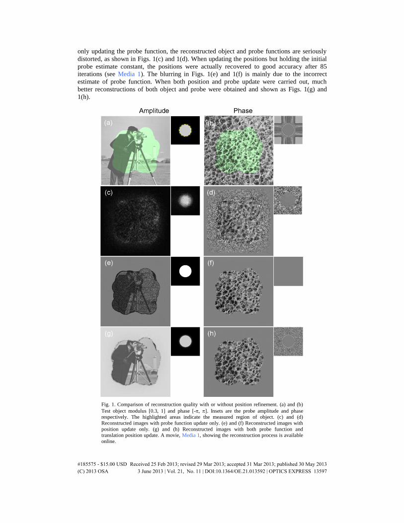
only updating the probe function, the reconstructed object and probe functions are seriously

distorted, as shown in Figs. 1(c) and 1(d). When updating the positions but holding the initial

probe estimate constant, the positions were actually recovered to good accuracy after 85

iterations (see Media 1). The blurring in Figs. 1(e) and 1(f) is mainly due to the incorrect

estimate of probe function. When both position and probe update were carried out, much

better reconstructions of both object and probe were obtained and shown as Figs. 1(g) and

1(h).

Fig. 1. Comparison of reconstruction quality with or without position refinement. (a) and (b)

Test object modulus [0.3, 1] and phase [-, ]. Insets are the probe amplitude and phase respectively. The highlighted areas indicate the measured region of object. (c) and (d)

Reconstructed images with probe function update only. (e) and (f) Reconstructed images with

position update only. (g) and (h) Reconstructed images with both probe function and translation position update. A movie, Media 1, showing the reconstruction process is available

online.


http://www.opticsinfobase.org/oe/viewmedia.cfm?uri=oe-21-11-13592-1


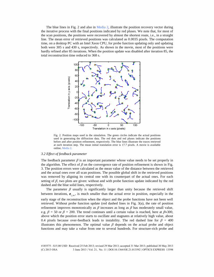
The blue lines in Fig. 2 and also in Media 2, illustrate the position recovery vector during

the iterative process with the final positions indicated by red pluses. We note that, for most of

the scan positions, the positions were recovered by almost the shortest route, i.e., in a straight

line. The mean error of retrieved positions was calculated as 0.0035 pixels. The computation

time, on a desktop PC with an Intel Xeon CPU, for probe function updating only and updating

both were 305 s and 430 s, respectively. As shown in the movie, most of the positions were

hardly refined after 85 iterations. When the position update was disabled after iteration 85, the

total reconstruction time reduced to 368 s.

Fig. 2. Position maps used in the simulation. The green circles indicate the actual positions

used in generating the diffraction data. The red dots and red pluses indicate the positions before and after position refinement, respectively. The blue lines illustrate the traces retrieved

at each iteration step. The mean initial translation error is 17.7 pixels. A movie is available

online, Media 2.

3.2 Effect of feedback parameter

The feedback parameter is an important parameter whose value needs to be set properly in

the algorithm. The effect of on the convergence rate of position refinement is shown in Fig.

3. The position errors were calculated as the mean value of the distance between the retrieved

and the actual ones over all scan positions. The possible global shift in the retrieved positions

was removed by aligning its central one with its counterpart of the actual ones. For each

setting of , two plots are given: without and with probe function update indicated by the red

dashed and the blue solid lines, respectively.

The parameter usually is significantly larger than unity because the retrieved shift

between iterations, mj ,e , is much smaller than the actual error in position, especially in the

early stage of the reconstruction when the object and the probe functions have not been well

retrieved. Without probe function update (red dashed lines in Fig. 3(a), the rate of position

refinement improves monotonically as increases as long as has moderately small value,

e.g. = 50 or = 200. The trend continues until a certain value is reached, here at 300,

above which the position error starts to oscillate and stagnates at relatively high value, about

0.4 pixels because over-feedback leads to instability. The red dashed line for = 400

illustrates this phenomenon. The optimal value depends on the actual probe and object

functions and may take a value from one to several hundreds. For structure-rich probe and




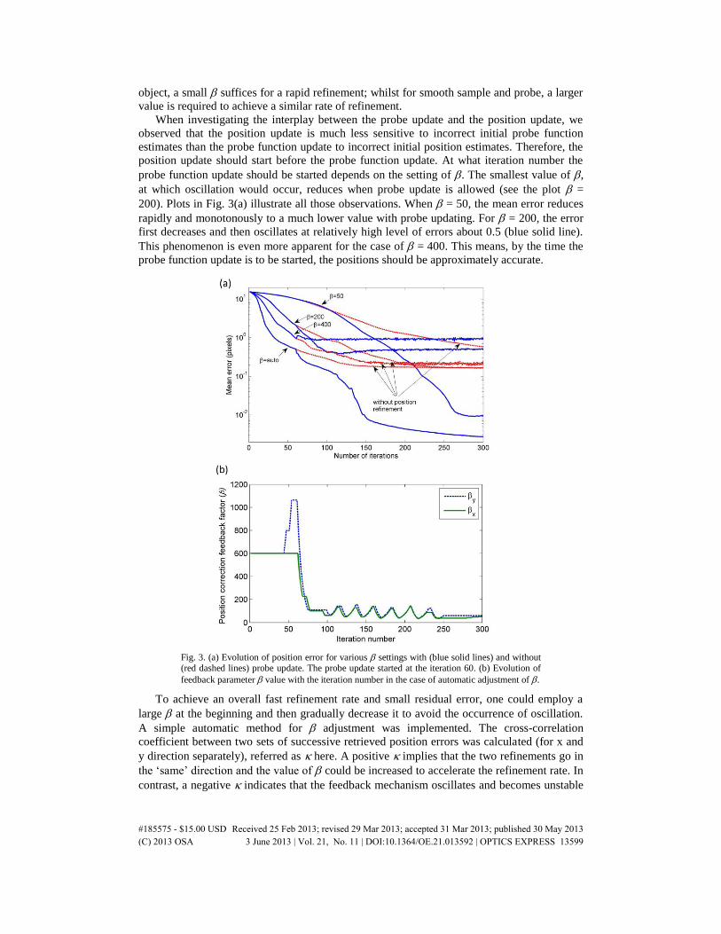
object, a small suffices for a rapid refinement; whilst for smooth sample and probe, a larger

value is required to achieve a similar rate of refinement.

When investigating the interplay between the probe update and the position update, we

observed that the position update is much less sensitive to incorrect initial probe function

estimates than the probe function update to incorrect initial position estimates. Therefore, the

position update should start before the probe function update. At what iteration number the

probe function update should be started depends on the setting of . The smallest value of ,

at which oscillation would occur, reduces when probe update is allowed (see the plot =

200). Plots in Fig. 3(a) illustrate all those observations. When = 50, the mean error reduces

rapidly and monotonously to a much lower value with probe updating. For = 200, the error

first decreases and then oscillates at relatively high level of errors about 0.5 (blue solid line).

This phenomenon is even more apparent for the case of = 400. This means, by the time the

probe function update is to be started, the positions should be approximately accurate.

Fig. 3. (a) Evolution of position error for various settings with (blue solid lines) and without (red dashed lines) probe update. The probe update started at the iteration 60. (b) Evolution of

feedback parameter value with the iteration number in the case of automatic adjustment of .

To achieve an overall fast refinement rate and small residual error, one could employ a

large at the beginning and then gradually decrease it to avoid the occurrence of oscillation.

A simple automatic method for adjustment was implemented. The cross-correlation

coefficient between two sets of successive retrieved position errors was calculated (for x and

y direction separately), referred as here. A positive implies that the two refinements go in

the ‘same’ direction and the value of could be increased to accelerate the refinement rate. In

contrast, a negative indicates that the feedback mechanism oscillates and becomes unstable


and the value of should be reduced. In our implementation, when was greater than 0.3,

was increased by 1.1 times to accelerate the refinement. When was less than 0.3, it was

decreased by a factor of 0.9. The actual value of the preset thresholds (here, ± 0.3) is not

critical. The improvement of using automatically adjusted is shown in Fig. 3(a). In the case

without probe function update, it reached the same error as with = 200 but at a much faster

rate. The remaining error is mainly due to the incorrect probe. When the probe function

update was allowed, a much lower position error, i.e., 0.0035 pixels was achieved. Plots in

Fig. 3(b) show the evolution of as the iteration progresses.

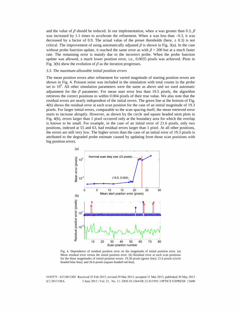
3.3. The maximum allowable initial position errors

The mean position errors after refinement for varied magnitude of starting position errors are

shown in Fig. 4. Poisson noise was included in the simulation with total counts in the probe

set to 108. All other simulation parameters were the same as above and we used automatic

adjustment for the parameter. For mean start error less than 19.5 pixels, the algorithm

retrieves the correct positions to within 0.004 pixels of their true value. We also note that the

residual errors are nearly independent of the initial errors. The green line at the bottom of Fig.

4(b) shows the residual error at each scan position for the case of an initial magnitude of 19.3

pixels. For larger initial errors, comparable to the scan spacing itself, the mean retrieved error

starts to increase abruptly. However, as shown by the circle and square headed stem plots in

Fig. 4(b), errors larger than 1 pixel occurred only at the boundary area for which the overlap

is known to be small. For example, in the case of an initial error of 21.6 pixels, only two

positions, indexed at 55 and 63, had residual errors larger than 1 pixel. At all other positions,

the errors are still very low. The higher errors than the case of an initial error of 19.3 pixels is

attributed to the degraded probe estimate caused by updating from those scan positions with

big position errors.

Fig. 4. Dependence of residual position error on the magnitude of initial position error. (a)

Mean residual error versus the initial position error. (b) Residual error at each scan positions for the three magnitudes of initial position errors: 19.28 pixels (green line); 21.6 pixels (circle

headed blue line); and 26.6 pixels (square headed red line).


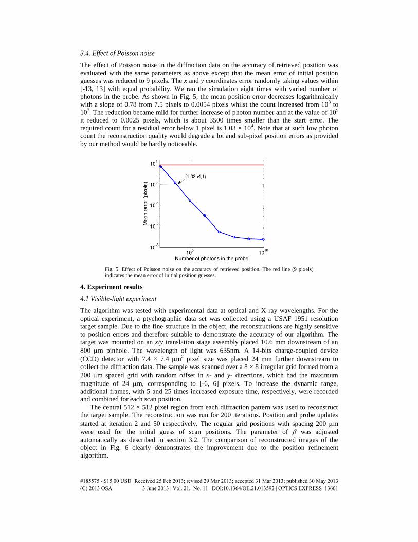
3.4. Effect of Poisson noise

The effect of Poisson noise in the diffraction data on the accuracy of retrieved position was

evaluated with the same parameters as above except that the mean error of initial position

guesses was reduced to 9 pixels. The x and y coordinates error randomly taking values within

[-13, 13] with equal probability. We ran the simulation eight times with varied number of

photons in the probe. As shown in Fig. 5, the mean position error decreases logarithmically

with a slope of 0.78 from 7.5 pixels to 0.0054 pixels whilst the count increased from 103 to

107. The reduction became mild for further increase of photon number and at the value of 10

9

it reduced to 0.0025 pixels, which is about 3500 times smaller than the start error. The

required count for a residual error below 1 pixel is 1.03 × 104. Note that at such low photon

count the reconstruction quality would degrade a lot and sub-pixel position errors as provided

by our method would be hardly noticeable.

Fig. 5. Effect of Poisson noise on the accuracy of retrieved position. The red line (9 pixels)

indicates the mean error of initial position guesses.

4. Experiment results

4.1 Visible-light experiment

The algorithm was tested with experimental data at optical and X-ray wavelengths. For the

optical experiment, a ptychographic data set was collected using a USAF 1951 resolution

target sample. Due to the fine structure in the object, the reconstructions are highly sensitive

to position errors and therefore suitable to demonstrate the accuracy of our algorithm. The

target was mounted on an x/y translation stage assembly placed 10.6 mm downstream of an

800 m pinhole. The wavelength of light was 635nm. A 14-bits charge-coupled device

(CCD) detector with 7.4 × 7.4 m2 pixel size was placed 24 mm further downstream to

collect the diffraction data. The sample was scanned over a 8 × 8 irregular grid formed from a

200 m spaced grid with random offset in x- and y- directions, which had the maximum

magnitude of 24 m, corresponding to [-6, 6] pixels. To increase the dynamic range,

additional frames, with 5 and 25 times increased exposure time, respectively, were recorded

and combined for each scan position.

The central 512 × 512 pixel region from each diffraction pattern was used to reconstruct

the target sample. The reconstruction was run for 200 iterations. Position and probe updates

started at iteration 2 and 50 respectively. The regular grid positions with spacing 200 m

were used for the initial guess of scan positions. The parameter of was adjusted

automatically as described in section 3.2. The comparison of reconstructed images of the

object in Fig. 6 clearly demonstrates the improvement due to the position refinement

algorithm.


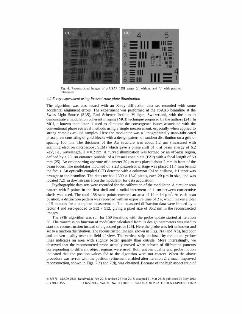
Fig. 6. Reconstructed images of a USAF 1951 target (a) without and (b) with position

refinement.

4.2 X-ray experiment using Fresnel zone plate illumination

The algorithm was also tested with an X-ray diffraction data set recorded with some

accidental alignment errors. The experiment was performed at the cSAXS beamline at the

Swiss Light Source (SLS), Paul Scherrer Institut, Villigen, Switzerland, with the aim to

demonstrate a modulation coherent imaging (MCI) technique proposed by the authors [24]. In

MCI, a known modulator is used to eliminate the convergence issues associated with the

conventional phase retrieval methods using a single measurement, especially when applied to

strong complex-valued samples. Here the modulator was a lithographically nano-fabricated

phase plate consisting of gold blocks with a design pattern of random distribution on a grid of

spacing 100 nm. The thickness of the Au structure was about 1.2 m (measured with

scanning electron microscopy, SEM) which gave a phase shift of at beam energy of 6.2

keV, i.e., wavelength, = 0.2 nm. A curved illumination was formed by an off-axis region,

defined by a 20 m entrance pinhole, of a Fresnel zone plate (FZP) with a focal length of 50

mm [25]. An order-sorting aperture of diameter 20 m was placed about 2 mm in front of the

beam focus. The modulator mounted on a 2D piezoelectric stage was placed 11.4 mm behind

the focus. An optically coupled CCD detector with a columnar CsI scintillator, 1:1 taper was

brought to the beamline. The detector had 1300 × 1340 pixels, each 20 m in size, and was

located 7.21 m downstream from the modulator for data acquisition.

Ptychographic data sets were recorded for the calibration of the modulator. A circular scan

pattern with 5 points in the first shell and a radial increment of 1 m between consecutive

shells was used. The total 158 scan points covered an area of 14 × 14 m2. At each scan

position, a diffraction pattern was recorded with an exposure time of 2 s, which makes a total

of 5 minutes for a complete measurement. The measured diffraction data were binned by a

factor 4 and zero-padded to 512 × 512, giving a pixel size of 35.2 nm in the reconstructed

images.

The ePIE algorithm was run for 150 iterations with the probe update started at iteration

50. The transmission function of modulator calculated from its design parameters was used to

start the reconstruction instead of a guessed probe [26]. Here the probe was left unknown and

set to a random distribution. The reconstructed images, shown in Figs. 7(a) and 7(b), had poor

and uneven quality over the field of view. The vertical strip enclosed by the dotted yellow

lines indicates an area with slightly better quality than outside. More interestingly, we

observed that the reconstructed probe actually moved when subsets of diffraction patterns

corresponding to different object regions were used. Both uneven quality and probe motion

indicated that the position values fed to the algorithm were not correct. When the above

procedure was re-run with the position refinement enabled after iteration 2, a much improved

reconstruction, shown in Figs. 7(c) and 7(d), was obtained. Because of the high aspect ratio of


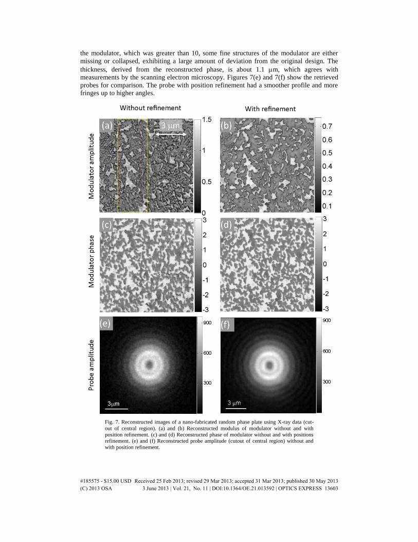
the modulator, which was greater than 10, some fine structures of the modulator are either

missing or collapsed, exhibiting a large amount of deviation from the original design. The

thickness, derived from the reconstructed phase, is about 1.1 m, which agrees with

measurements by the scanning electron microscopy. Figures 7(e) and 7(f) show the retrieved

probes for comparison. The probe with position refinement had a smoother profile and more

fringes up to higher angles.

Fig. 7. Reconstructed images of a nano-fabricated random phase plate using X-ray data (cut-

out of central region). (a) and (b) Reconstructed modulus of modulator without and with

position refinement. (c) and (d) Reconstructed phase of modulator without and with positions refinement. (e) and (f) Reconstructed probe amplitude (cutout of central region) without and

with position refinement.


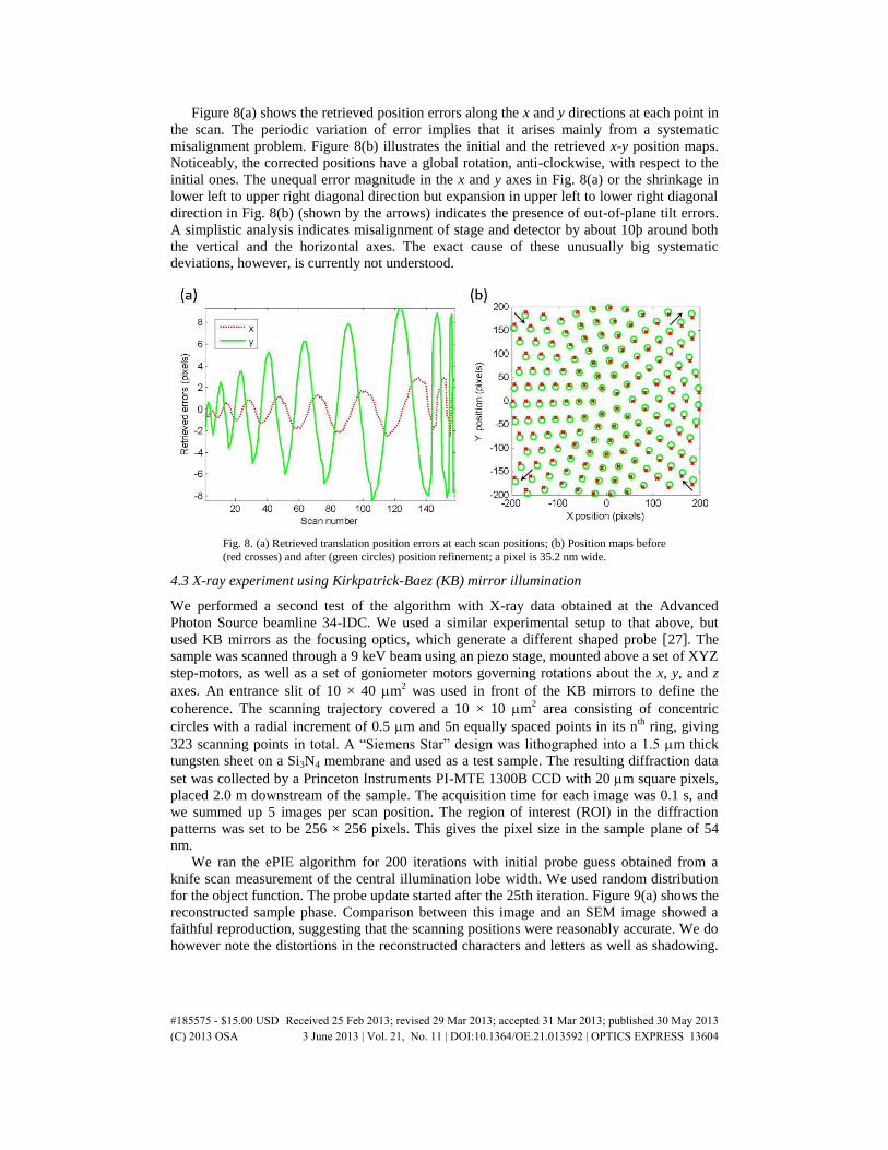
Figure 8(a) shows the retrieved position errors along the x and y directions at each point in

the scan. The periodic variation of error implies that it arises mainly from a systematic

misalignment problem. Figure 8(b) illustrates the initial and the retrieved x-y position maps.

Noticeably, the corrected positions have a global rotation, anti-clockwise, with respect to the

initial ones. The unequal error magnitude in the x and y axes in Fig. 8(a) or the shrinkage in

lower left to upper right diagonal direction but expansion in upper left to lower right diagonal

direction in Fig. 8(b) (shown by the arrows) indicates the presence of out-of-plane tilt errors.

A simplistic analysis indicates misalignment of stage and detector by about 10þ around both

the vertical and the horizontal axes. The exact cause of these unusually big systematic

deviations, however, is currently not understood.

Fig. 8. (a) Retrieved translation position errors at each scan positions; (b) Position maps before

(red crosses) and after (green circles) position refinement; a pixel is 35.2 nm wide.

4.3 X-ray experiment using Kirkpatrick-Baez (KB) mirror illumination

We performed a second test of the algorithm with X-ray data obtained at the Advanced

Photon Source beamline 34-IDC. We used a similar experimental setup to that above, but

used KB mirrors as the focusing optics, which generate a different shaped probe [27]. The

sample was scanned through a 9 keV beam using an piezo stage, mounted above a set of XYZ

step-motors, as well as a set of goniometer motors governing rotations about the x, y, and z

axes. An entrance slit of 10 × 40 m2 was used in front of the KB mirrors to define the

coherence. The scanning trajectory covered a 10 × 10 m2 area consisting of concentric

circles with a radial increment of 0.5 m and 5n equally spaced points in its nth

ring, giving

323 scanning points in total. A “Siemens Star” design was lithographed into a 1.5 m thick

tungsten sheet on a Si3N4 membrane and used as a test sample. The resulting diffraction data

set was collected by a Princeton Instruments PI-MTE 1300B CCD with 20 m square pixels,

placed 2.0 m downstream of the sample. The acquisition time for each image was 0.1 s, and

we summed up 5 images per scan position. The region of interest (ROI) in the diffraction

patterns was set to be 256 × 256 pixels. This gives the pixel size in the sample plane of 54

nm.

We ran the ePIE algorithm for 200 iterations with initial probe guess obtained from a

knife scan measurement of the central illumination lobe width. We used random distribution

for the object function. The probe update started after the 25th iteration. Figure 9(a) shows the

reconstructed sample phase. Comparison between this image and an SEM image showed a

faithful reproduction, suggesting that the scanning positions were reasonably accurate. We do

however note the distortions in the reconstructed characters and letters as well as shadowing.


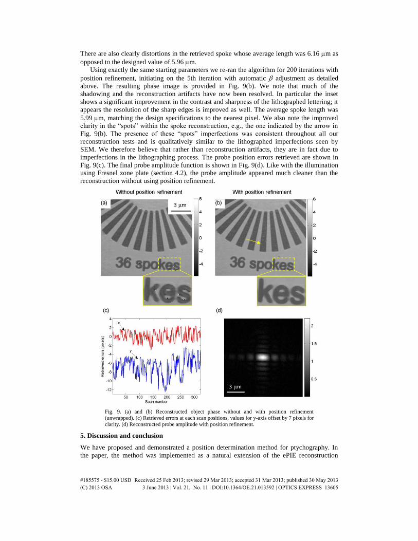
There are also clearly distortions in the retrieved spoke whose average length was 6.16 m as

opposed to the designed value of 5.96 m.

Using exactly the same starting parameters we re-ran the algorithm for 200 iterations with

position refinement, initiating on the 5th iteration with automatic adjustment as detailed

above. The resulting phase image is provided in Fig. 9(b). We note that much of the

shadowing and the reconstruction artifacts have now been resolved. In particular the inset

shows a significant improvement in the contrast and sharpness of the lithographed lettering; it

appears the resolution of the sharp edges is improved as well. The average spoke length was

5.99 m, matching the design specifications to the nearest pixel. We also note the improved

clarity in the “spots” within the spoke reconstruction, e.g., the one indicated by the arrow in

Fig. 9(b). The presence of these “spots” imperfections was consistent throughout all our

reconstruction tests and is qualitatively similar to the lithographed imperfections seen by

SEM. We therefore believe that rather than reconstruction artifacts, they are in fact due to

imperfections in the lithographing process. The probe position errors retrieved are shown in

Fig. 9(c). The final probe amplitude function is shown in Fig. 9(d). Like with the illumination

using Fresnel zone plate (section 4.2), the probe amplitude appeared much cleaner than the

reconstruction without using position refinement.

Fig. 9. (a) and (b) Reconstructed object phase without and with position refinement

(unwrapped). (c) Retrieved errors at each scan positions, values for y-axis offset by 7 pixels for

clarity. (d) Reconstructed probe amplitude with position refinement.

5. Discussion and conclusion

We have proposed and demonstrated a position determination method for ptychography. In

the paper, the method was implemented as a natural extension of the ePIE reconstruction


algorithm. The accuracy of the algorithm is determined by how accurately the cross

correlation can be performed. This in turn is determined by the actual probe and object

functions, the overlap ratio between measurements and the noise level in the data. For objects

lacking fine structure, the cross correlation calculation would become less sensitive to the

position errors. On the other hand, for such objects, the reconstruction quality will also be

more tolerant to position errors. In simulation, our position refinement mechanism has been

able to retrieve the sample positions to within a few thousandths’ of a pixel accuracy in just

several tens of iterations.

The two examples using X-ray data from SLS and APS, using different samples and

different kinds of probe, both showed significant improvement of image quality of both object

and probe, but with slightly different characteristics. In the SLS case the probe positions arose

mainly from a misalignment of the scanning axis directions and the pixel directions of the

detector. This is not easy to align in general, but our result indicates that it is important to pay

attention to this aspect in the experimental setup. In the APS case, the position errors in Fig.

9(c) had still systematic local variations in which neighbouring scanning positions appear to

move together but without the overall rotations found in the first experiment. This might

indicate there are linearity issues with the piezo scanners. It is possible that the errors are due

to “wobble” motions aggravated by the fact that the encoders of the scan stage are in a

different plane from the sample.

In our simulations, early tests suggest that it would be possible to retrieve the translation

positions starting from all-zeros guesses using this algorithm and we are investigating this

possibility, which could be important for applications such as high resolution metrology.

When applying the algorithm to real data, we found that for the algorithm to reliably retrieve

the correct positions, the degree of illumination coherence needs to be high. This is

understandable since the reconstruction from any coherent component within a partial

coherent diffraction data will appear at different scales (temporal partial coherence) or

different locations (spatial partial coherence), which would hinder the position error signal

finding by cross-correlation. We are currently working on modifying our algorithm to account

for partially coherent data to extend its applicability to a broader range of experimental

conditions [28].

We believe the proposed method offers a way to exploit the full resolution potential of

ptychographic coherent diffractive imaging. The main application of the method would be at

short wavelengths where position errors due to system instability and inaccuracy of

translation stages would become significant compared to the desired resolution. As shown in

our experiments, the method also improves results at longer wavelengths where systematic

errors due to misalignment are an issue.

Acknowledgments

The work was supported by the EPSRC basic technology grant under the project Ultimate

Microscope (EP/E034055/1) and in part by the EPSRC grant (EP/I022562/1), the Phase

Modulation Technology for X-ray Imaging. The X-ray measurements were made at the Swiss

Light Source, Paul Scherrer Institute, Villigen, Switzerland, and at APS beamline 34-ID-C,

built with US National Science Foundation grant DMR-9724294 and operated by the US

Department of Energy, Office of Basic Energy Sciences, under contract no. DE-

AC0206CH11357. I.P. is supported by the Australian Research Council Centre of Excellence

for Coherent X-ray Science. R.B. acknowledges travel support from the European

Community’s Seventh Framework Programme (FP7/2007–2013) through grant no. 226716.

We would like to thank Mirko Holler for fruitful discussions and Manuel Guizar-Sicairos for

critical reading of the manuscript and helpful comments.


Translation position determination in ptychographic coherent diffraction imaging

Documents