Transient heat-conduction-Part-I

Lectures on Heat Transfer -- TRANSIENT HEAT

CONDUCTION: Part-I

by

Dr. M. Thirumaleshwar

formerly:

Professor, Dept. of Mechanical Engineering,

St. Joseph Engg. College, Vamanjoor,

Mangalore

India

Preface

• This file contains slides on Transient Heat

conduction: Part-I

• The slides were prepared while teaching

Heat Transfer course to the M.Tech.

students in Mechanical Engineering Dept.

of St. Joseph Engineering College,

Vamanjoor, Mangalore, India, during Sept.

– Dec. 2010.

Aug. 2016 2 MT/SJEC/M.Tech.

• It is hoped that these Slides will be useful to teachers, students, researchers and professionals working in this field.

• For students, it should be particularly useful to study, quickly review the subject, and to prepare for the examinations.

• M. Thirumaleshwar August 2016

Aug. 2016 3 MT/SJEC/M.Tech.

Aug. 2016 MT/SJEC/M.Tech. 4

References

• 1. M. Thirumaleshwar: Fundamentals of Heat &

Mass Transfer, Pearson Edu., 2006 • https://books.google.co.in/books?id=b2238B-

AsqcC&printsec=frontcover&source=gbs_atb#v=onepage&q&f=false

• 2. Cengel Y. A. Heat Transfer: A Practical

Approach, 2nd Ed. McGraw Hill Co., 2003

• 3. Cengel, Y. A. and Ghajar, A. J., Heat and

Mass Transfer - Fundamentals and Applications,

5th Ed., McGraw-Hill, New York, NY, 2014.

https://books.google.co.in/books?id=b2238B-AsqcC&printsec=frontcover&source=gbs_atb#v=onepage&q&f=false



References… contd. • 4. Incropera , Dewitt, Bergman, Lavine:

Fundamentals of Heat and Mass Transfer, 6th

Ed., Wiley Intl.

• 5. M. Thirumaleshwar: Software Solutions to

Problems on Heat Transfer – CONDUCTION-

Part-II, Bookboon, 2013

• http://bookboon.com/en/software-solutions-problems-on-heat-

transfer-cii-ebook



TRANSIENT HEAT CONDUCTION: Part-I ..

Outline:

• Lumped system analysis – criteria for

lumped system analysis – Biot and Fourier

Numbers – Response time of a

thermocouple - One-dimensional transient

conduction in large plane walls, long

cylinders and spheres when Bi > 0.1 –

one-term approximation - Heisler and

Grober charts- Problems


TRANSIENT HEAT CONDUCTION:

• In transient conduction, temperature depends not only on position in the solid, but also on time.

• So, mathematically, this can be written as T = T(x,y,z,), where represents the time coordinate.

• Typical examples of transient conduction:

• heat exchangers

• boiler tubes

• cooling of I.C.Engine cylinder heads


Examples (contd.):

• heat treatment of engineering

components and quenching of ingots

• heating of electric irons

• heating and cooling of buildings

• freezing of foods, etc.


Lumped system analysis

(Newtonian heating or cooling):

• In lumped system analysis, the internal conduction resistance of the body to heat flow (i.e. L/(k.A)) is negligible compared to the convective resistance (i.e. 1/(h.A)) at the surface.

• So, the temperature of the body, no doubt, varies with time, but at any given instant, the temperature within the body is uniform and is independent of position. i.e. T = T() only.


Lumped system analysis

(Newtonian heating or cooling):

• Practical examples of such cases are:

heat treatment of small metal pieces,

measurement of temperature with a

thermocouple or thermometer etc, where

the internal resistance of the object for

heat conduction may be considered as

negligible.


Analysis:

• Consider a solid body of arbitrary shape, volume V,

mass m, density , surface area A, and specific heat

Cp. See Fig. 7.1.

• To start with, at = 0, let the temperature throughout

the body be uniform at T = Ti. At the instant = 0, let

the body be suddenly placed in a medium at a

temperature of Ta, as shown.


• Writing an energy balance for this situation:

• Amount of heat transferred into the body in time

interval d =

Increase in the internal energy of the body in

time interval d

i .e. h A T a T ( ) d m C p dT C p

V dT ....(7.1) since m = . V

Now, since Ta is a constant, we can write: dT d T ( ) T a

Therefore,

d T ( ) T a

T ( ) T a

h A

C p V

d .....(7.2)


Integrating between = 0 (i.e. T = Ti) and

any , (i.e. T = T()),

lnT ( ) T a

T i T a

h A

C p V

i.e.T ( ) T a

T i T a

exph A

C p V

......(7.3)


• Now, let:

C p V

h At

where, ‘t’ is known as ‘thermal time constant’ and has

units of time.

Therefore, eqn. (7.3) is written as:

T ( ) T a

T i T a

exp

t.......(7.4)

Now denoting θ = (T() – Ta), we write eqn. (7.4)

compactly as:


i

T ( ) T a

T i T a

exp

t......(7.5)

Equation (7.5) gives the temperature distribution in a

solid as a function of time, when the internal resistance

of the solid for conduction is negligible compared to the

convective resistance at its surface. See Fig. 7.2 (a)



• Instantaneous heat Transfer:

• At any instant , heat transfer between the body and the

environment is easily calculated since we have the

temperature distribution from eqn. (7.4):

Q ( ) m C p dT ( )

d W......(7.6,a)

At that instant, heat transfer must also be equal to:

Q ( ) h A T ( ) T a W.....(7.6,b)

Total heat transfer:

Total heat transferred during = 0 to = , is equal to

the change in Internal energy of the body:

Q tot m C p T ( ) T i

J....(7.7,a)


• Qtot may also be calculated by integrating eqn.(7.6,a):

Q tot0

Q ( ) d J.....(7.7,b)

Max. heat transferred:

When the body reaches the temperature of the environment,

obviously maximum heat has been transferred:

Q max m C p T a T i

J.....(7.8)

If Qmax is negative, it means that the body has lost heat,

and if Qmax is positive, then body has gained heat.


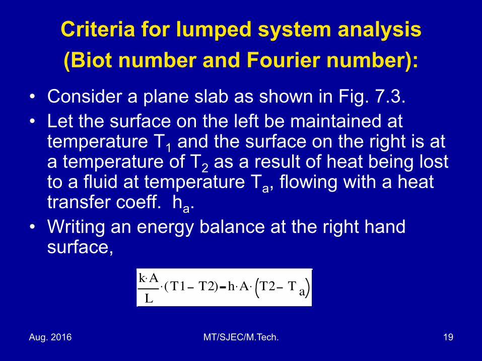
Criteria for lumped system analysis

(Biot number and Fourier number):

• Consider a plane slab as shown in Fig. 7.3.

• Let the surface on the left be maintained at temperature T1 and the surface on the right is at a temperature of T2 as a result of heat being lost to a fluid at temperature Ta, flowing with a heat transfer coeff. ha.

• Writing an energy balance at the right hand surface,

k A

LT1 T2( ) h A T2 T a


Criteria for lumped system analysis

(Biot number and Fourier number):

Rearranging,

T1 T2

T2 T a

L

k A

1

h A

R cond

R conv

h L

kBi ......(7.9)

The term, (h.L)/k, appearing on the RHS of

eqn. (7.9) is a dimensionless number, known

as ‘Biot number’.


Fig. 7.3(a) Biot number and temp. distribution in a plane wall

h, T a

X

T1T2

T2

T2

Ta

Bi << 1

Bi = 1Bi >> 1

QconvQcond

L


• Note from Fig. (7.3, a) the temperature profile for

Bi << 1.

• It suggests that one can assume a uniform temperature

distribution within the solid if Bi << 1.

• Situation during transient conduction is shown in Fig.

(7.3,b). It may be observed hat temperature distribution

is a strong function of Biot number.

Fig. 7.3(b) Biot number and transient temp. distribution in a plane wall

h, T a

Bi << 1 Bi = 1 Bi >> 1

T(x,0) = Ti T(x,0) = Ti


• For Bi << 1, temperature gradient in the solid is

small and temperature can be taken as a

function of time only.

• Note also that for Bi >> 1, temperature drop

across the solid is much larger than that across

the convective layer at the surface.

• Let us define Biot number, in general, as follows:

Bih L c

k.....(7.10)


where, h is the heat transfer coeff. between

the solid surface and the surroundings, k is

the thermal conductivity of the solid, and Lc

is a characteristic length defined as the ratio

of the volume of the body to its surface area,

i.e.

L cV

A


• For solids such as a plane slab, long cylinder and

sphere, it is found that transient temperature distribution

within the solid at any instant is uniform, with the error

being less than about 5%, if the following criterion is

satisfied: Bi

h L c

k0.1 ......(7.11)

Lc for common shapes:

(i) Plane wall (thickness 2L): L cA 2 L

2 AL = half thickness of wall

(i i) Long cylinder, radius, R: L c R

2 L

2 R LR

2

(i i i) Sphere, radius, R: L c

4

3 R

3

4 R2

R

3

(iv) Cube, side L: L cL

3

6 L2

L

6


• Therefore, we can write eqn. (7.3) as:

i

T ( ) T a

T i T a

exph A

C p V

i f Bi < 0.1.....(7.12)

Eqn. (7.12) is important.

Its application to a given problem is very simple and solution

of any transient conduction problem must begin with

examining if the criterion, Bi < 0.1 is satisfied to see if

eqn. (7.12) could be applied.

Now, the term (hA)/(Cp V) can be written as follows:

h A

C p V

h L c

k

k

C p L c

2

h L c

k

L c2

Bi Fo

where, Fo

L c2

= Fourier number, or relative time


• Fourier number, like Biot number, is an

important parameter in transient heat

transfer problems.

• It is also known as ‘dimensionless time’. • Fourier number signifies the degree of

penetration of heating or cooling effect

through a solid.

• For small Fo, large will be required to get

significant temperature changes.


• Now, we can rewrite eqn. (7.12) as:

i

T ( ) T a

T i T a

exp Bi Fo( ) i f Bi < 0.1.....(7.13)

Eqn. (7.13) is plotted in Fig. (7.4) below.

Remember that this graph is for the cases

where lumped system analysis is applicable,

i.e. Bi < 0.1.


Let X Bi Fo

X 0 0.1 5

Then

i

exp X( )

exp X( )

X

0 0.5 1 1.5 2 2.5 3 3.5 4 4.5 51 10

3

0.01

0.1

1

Transient temp.distrib.in solids, Bi<0.1

Fig. (7.4) Dimensionless temperature distribution in solids during transient h

transfer, (Bi < 0.1)--for lumped system analysis


Response time of a thermocouple:

• Lumped system analysis is usefully

applied in the case of temperature

measurement with a thermometer or a

thermocouple. Obviously, it is desirable

that the thermocouple indicates the source

temperature as fast as possible.

• ‘Response time’ of a thermocouple is

defined as the time taken by it to reach the

source temperature.


Response time of a thermocouple:

• Consider eqn. (7.12):

i

T ( ) T a

T i T a

exph A

C p V

i f Bi < 0.1.....(7.12)

For rapid response, the term (h A )/( Cp V)

should be large so that the exponential term will

reach zero faster. This means that:

(i) increase (A/V), i.e. decrease the wire

diameter

(ii) decrease density and specific heat, and

(iii) increase the value of heat transfer coeff. h


• The quantity ( Cp V)/(h A) is known as ‘thermal time constant’, t, of the measuring system and has units of

time.

• At = t i.e. at a time interval of one time constant, we

have:

T ( ) T a

T i T a

e1

0.368 .....(7.14)

From eqn. (7.14), it is clear that after an interval of time

equal to one time constant of the given temperature

measuring system, the temperature difference between the

body (thermocouple) and the source would be 36.8% of

the initial temperature difference. i.e. the temperature

difference would be reduced by 63.2%.


Time required by a thermocouple to attain

63.2% of the value of initial temperature

difference is called its ‘sensitivity’.

For good response, obviously the response

time of thermocouple should be low.

As a thumb rule, it is recommended that while

using a thermocouple to measure temperatures,

reading of the thermocouple should be taken

after a time equal to about four time periods has

elapsed.


• Example 7.1 (M.U.): A steel ball 5 cm dia, initially at an uniform temperature of 450 C is suddenly placed in an environment at 100 C. Heat transfer coeff. h, between the steel ball and the fluid is 10 W/(m2.K). For steel, cp = 0.46 kJ/(kg.K), ρ = 7800 kg/m3, k = 35 W/(m.K). Calculate the time required for the ball to reach a temperature of 150 C. Also find the rate of cooling after 1 hr. Show graphically how the temp. of the sphere falls with time.



• First, calculate the Biot number:

Since Bi < 0.1, lumped system analysis is applicable, and the

temperature variation within the solid will be within an error of 5%.

Applying eqn. (7.12), we get:

i

T ( ) T a

T i T a

exph A

C p V

i f Bi < 0.1.....(7.12)

i .e.T T a

T i T a

exp

twhere t is the time constant.


• And, time constant is given by:

t c p V

A h

c p

h

R

3

..since for sphere, V/A = R/3

i .e. t c p

h

R

3

...define time constant, t

i .e. t 2990 s....time constant

Therefore, we write:

150 100

450 100exp

2990where is the time required to reach 150 C


i .e. ln50

350

2990

or, 2990 ln50

350

s....define , the time reqd. to reach 150 C

i.e. 5.818103 s... time reqd. to reach 150 C...Ans.

i .e. 1.616 hrs.....Ans

Rate of cooling after 1 hr.:

i .e. 3600 s

From eqn. (7.12), we have:

T ( ) T i T a exph A

c p V

T a ....define T()


i .e.dT

dT i T a

h A

V c p

exph A

V c p

C/s.....rate of cooling

T ( )

d

d0.035 C/s....rate of cooling after 1 hr..Ans.

i .e.

-ve sign indicates that as time increases, temperature falls.

To sketch the fall in temp. of sphere with time:

Temp. as a function of time is given by eqn. (7.12):

i

T ( ) T a

T i T a

exph A

c p V

i f Bi < 0.1.....(7.12)

i .e. T ( ) T a T i T a exph A

c p V

....eqn. (A)


• We will plot eqn. (A) against different times, :

T 3600( )

0 0.5 1 1.5 2 2.5 3 3.5 4

100

150

200

250

300

350

400

450

500

Trans. cooling of sphere-lumped system

in hrs. and T() in deg.C

Fig. Ex. 7.1 Transient cooling of a sphere considred as a lumped system

Note from the fig. how the cooling progresses with time.

After about 4 hrs. duration, the sphere approaches the temp.

of the ambient.

You can also verify from the graph that the time required for the

sphere to reach 150 C is 1.616 hrs, as calculated earlier.


• Example 7.4 (M.U.): A Thermocouple (TC)

junction is in the form of 8 mm sphere.

Properties of the material are: cp = 420 J/(kg.

K), ρ = 8000 kg/m3, k = 40 W/(m.K), and heat

transfer coeff., h = 45 W/(m2.K). Find, if the

junction is initially at a temp. of 28 C and

inserted in a stream of hot air at 300 C:

(i) the time const. of the TC

(ii) The TC is taken out from the hot air after

10 s and kept in still air at 30 C. Assuming ‘h’ in air as 10 W/(m2.K), find the temp. attained

by the junction 15 s after removing from hot

air stream.



• First, calculate the Biot number:

Bih L c

k

h

k

V

A

h

k

4

3( ) R

3

4 R2

i .e. Bih

k

R

3

...define Biot number

i.e. Bi 1.5 103 ...Biot number

Since Bi < 0.1, lumped system analysis is applicable, and the

temperature variation within the solid will be within an error of 5%.

See Fig. Ex. 7.4 (a).

Time constant is given by:

t c p V

A h

c p

h

R

3

..since for sphere, V/A = R/3

i.e. t c p

h

R

3


i .e. t 99.556 s....time constant.....Ans.


Fig. Ex.7.4 (a) Temperature measurement, with thermocoupleplaced in the air stream

Ta = 300 Ch = 45 W/(m2.K)

Thermocouple, D = 8 mm

Ti = 28 C

Air


• Temp. of TC after 10s:

10 s....time duration for which TC is kept in the stream at 300 C

We use eqn. (7.12). i .e.

i

T ( ) T a

T i T a

exph A

C p V

i f Bi < 0.1.....(7.12)

i .e.T T a

T i T a

exp

twhere t is the time constant.

Therefore, T T i T a exp

t

T a C....define temp. of TC after 10 s in the

stream

i .e. T 53.994 C....temp. of TC 10 s after i t is placed in the stream at 300

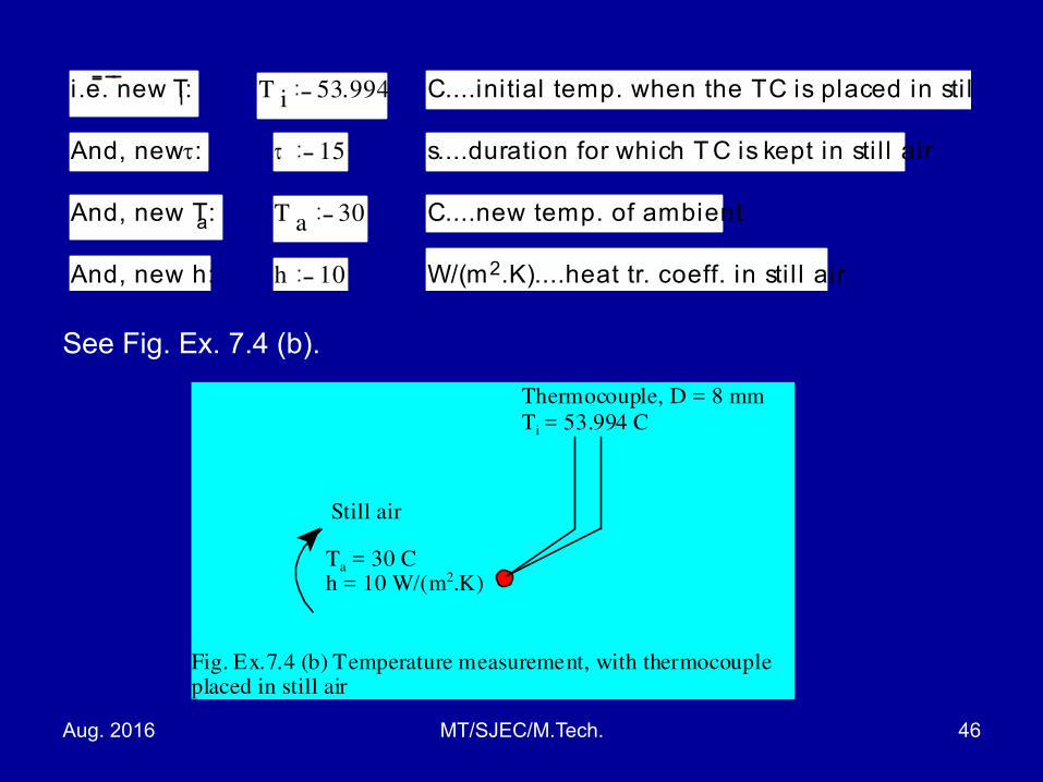
(b) Now, this TC is removed from the stream at 300 C and placed

in still air at 30 C. So, the temp. of 53.994C becomes initial temp. Ti

for this case:


i .e. new Ti: T i 53.994 C....initial temp. when the TC is placed in sti l l

And, new : 15 s....duration for which T C is kept in sti l l air

And, new Ta: T a 30 C....new temp. of ambient

And, new h: h 10 W/(m2.K)....heat tr. coeff. in sti l l air

See Fig. Ex. 7.4 (b).

Fig. Ex.7.4 (b) Temperature measurement, with thermocoupleplaced in still air

Ta = 30 Ch = 10 W/(m2.K)

Thermocouple, D = 8 mm

Ti = 53.994 C

Still air


And, new time constant:

i .e. t c p

h

R

3


i .e. t 448 s....time constant

Therefore, T T i T a exp

t

T a C....define temp. of T C after 15 s in sti l l a

i.e. T 53.204 C....temp. of TC 15 s after it is placed in still air

at 30 C...Ans.


One-dimensional transient conduction in large

plane walls, long cylinders and spheres when

Biot number > 0.1:

• When the temperature gradient in the solid is not negligible (i.e. Bi > 0.1), lumped system analysis is not applicable.

• One term approximation solutions:

• Fig. 7.6 shows schematic diagram and coordinate systems for a large, plane slab, long cylinder and a sphere.

• Consider a plane slab of thickness 2L, shown in Fig (a) above. Initially, i.e. at = 0, the slab is at an uniform temperature, Ti.


One-dimensional transient conduction in large

plane walls, long cylinders and spheres when

Biot number > 0.1:

• Suddenly, at = 0, both the surfaces of the slab are subjected to convection heat transfer with an ambient at temperature Ta , with a heat transfer coeff. h, as shown.

• Because of symmetry, we need to consider only half the slab, and that is the reason why we chose the origin of the coordinate system on the mid-plane.

• Then, we can write the mathematical formulation of the problem for plane slab as follows:



d2

T

dx2

1

dT

d in 0< x <L, for > 0.......(7.23, a)

dT

dx0 at x = 0, for > 0.......(7.23, b)

kdT

dx

h T T a at x = L, for > 0 ......(7.23, c)

T T i for = 0, in 0 < x < L .....(7.23, d)

The solution of the above problem, however, is rather

involved and consists of infinite series. So, it is more

convenient to present the solution either in tabular form or

charts. For this purpose, we define the following dimensionless parameters:


• While using the tabular or chart solutions, note one

important difference in defining Biot number:

• Characteristic length in Biot number is taken as half

thickness L for a plane wall, Radius R for a long

cylinder and sphere instead of being calculated as

V/A, as done in lumped system analysis.

(i) Dimensionless temperature:

x ( )T x ( ) T a

T i T a

(ii) Dimensionless distance from the centre:

X

x

L

(iii) Dimensionless heat transfer coefficient:

Bih L

k...Biot number

(iv) Dimensionless time:

Fo

L2

....Fourier number


• It is observed that for Fo > 0.2, considering only the first

term of the series and neglecting other terms, involves

an error of less than 2%.

• Generally, we are interested in times, Fo > 0.2.

• So, it becomes very useful and convenient to use one

term approximation solution, for all these three cases,

as follows:

Plane wall: x ( )T x ( ) T a

T i T a

A 1 e 1

2Fo

cos 1 x

L

...Fo > 0.2....(7.24, a)

Long cylinder: x ( )T r ( ) T a

T i T a

A 1 e 1

2Fo

J 0

1 r

R

...Fo > 0.2....(7.24, b)

sphere: x ( )T r ( ) T a

T i T a

A 1 e 1

2Fo

sin

1 r

R

1 r

R

...Fo > 0.2....(7.24, c)


• In the above equations, A1 and λ1 are functions of Biot

number only.

• A1 and λ1 are calculated from the following relations:

(Values are available in Tables, Ref: Cengel)

Functions J0 and J1are the zeroth and first order Bessel functions of

the first kind, available from Handbooks.



• Now, at the centre of a plane wall, cylinder and sphere,

we have the condition x = 0 or r = 0.

• Then, noting that cos(0) = 1, J0 (0) = 1, and limit of

sin(x)/x is also 1, eqns. (7.24) become:

• At the centre of plane wall, cylinder and sphere:

Centre of plane wall:

(x = 0)

0

T 0 T a

T i T a

A 1 e 1

2Fo

....(7.25, a)

Centre of long cylinder:

(r = 0)

0

T 0 T a

T i T a

A 1 e 1

2Fo

...(7.25, b)

Centre of sphere:

(r = 0)

0

T 0 T a

T i T a

A 1 e 1

2Fo

...(7.25, c)


• The one-term solutions are presented in chart form in the next section.

• But, generally, it is difficult to read these charts accurately.

• So, relations given in eqns. (7.24) and (7.25) along with Tables for A1 and λ1 should be preferred to the charts.

Therefore, first step in the solution is to

calculate the Biot number;

• Once the Biot number is known, constants A1

and λ1 are found out from Tables and then use

relations given in eqns. (7.24) and (7.25) to

calculate the temperature at any desired

location.


• Calculation of amount of heat

transferred, Q:

• Let Q be the amount of heat lost (or gained) by

the body, during the time interval = 0 to = , i.e. from the beginning upto a given time.

• Let Qmax be the maximum possible heat transfer.

• Obviously, maximum amount of heat has

been transferred when the body has

reached equilibrium with the ambient.


• i.e.

Q max V C p T i T a

m C p T i T a

J.....(7.26)

where is the density, V is the volume, (V) is the mass,

Cp is the specific heat of the body.

Based on the one term approximation discussed above,

(Q/ Qmax) is calculated for the three cases, from the

following:

Plane wall:Q

Q max

1 0

sin 1

1

......(7.27, a)

Cylinder:Q

Q max

1 2 0

J 1 1

1

.....(7.27, b)

Sphere:Q

Q max

1 3 0

sin 1 1 cos 1

13

.....(7.27, c)


• Note:

• (i) Remember well the definition of Biot number- i.e. Bi = (hL/k), where L is half thickness of the slab, and Bi = (hR/k), where R is the outer radius of the cylinder or the

sphere. • (ii) Foregoing results are equally applicable to

a plane wall of thickness L, insulated on one side and suddenly subjected to convection at the other side. This is so because, the boundary condition dT/dx = 0 at x = 0 for the mid-plane of a slab of thickness 2L (see eqn. 7.23, b), is equally applicable to a slab of thickness L, insulated at x = 0.


• Note (contd.):

• (iii) These results are also applicable to determine the temperature response of a body when temperature of its surface is suddenly changed to Ts . This case is equivalent to having convection at the surface with a heat transfer coeff., h = ∞;

now, Ta is replaced by the prescribed surface temperature, Ts.

• Remember that these results are valid for the situation where Fourier number, Fo > 0.2.


Heisler and Grober charts:

• The one term approximation solutions

(eqn. (7.25)) were represented in graphical

form by Heisler in 1947. They were

supplemented by Grober in 1961, with

graphs for heat transfer (eqn. (7.27)).

• These graphs are shown in following

slides for plane wall, long cylinder and a

sphere, respectively.


Heisler and Grober charts:

• About the charts:

• First chart in each of these figures gives the non-

dimensionalised centre temperature T0. i.e. at x

= 0 for the slab of thickness 2L, and at r = 0 for

the cylinder and sphere, at a given time . • Temperature at any other position at the same

time , is calculated using the next graph, called

‘position correction chart’. • Third chart gives Q/Qmax.


Temperature of Plate at mid-plane:


Temperature of Plate at any plane:


Heat transfer for Plate:


Temperature of Cylinder at mid-point:


Temperature of Cylinder at any radius:


Heat transfer for Cylinder:


Temperature of Sphere at mid-point:


Temperature of Sphere at any radius:


Heat transfer for Sphere:


How to use these charts? • Procedure of using these charts to solve

a numerical problem is as follows:

• First of all, calculate Bi from the data, with the

usual definition of Bi i.e. Bi = (h.Lc)/k, where Lc

is the characteristic dimension, given as: Lc =

(V/A).

• i.e. Lc = L, half-thickness for a plane wall, Lc =

R/2 for a cylinder, and Lc=R/3 for a sphere.

• If Bi < 0.1, use lumped system analysis;

otherwise, go for one term approx. or chart

solution.


How to use these charts? • If Bi > 0.1, calculate the Biot number

again with the appropriate definition of Bi i.e. Bi =(hL/k) for a plane wall where L is half-thickness, and Bi = (hR/k) for a cylinder or sphere, where R is the outer radius. Also, calculate Fourier number, Fo = ./L2 for the plane wall, and Fo = ./R2 for a cylinder or sphere.

• To calculate the centre temperature, use the first chart in the set given, depending upon the geometry being considered.


• Fo is on the x-axis; draw a vertical line to intersect the

(1/Bi) line; from the point of intersection, move

horizontally to the left to the y-axis to read the value of

o = (To –Ta)/(Ti – Ta). Here, To is the centre

temperature, which can now be calculated since Ti

and Ta are known.

• To calculate the temperature at any other position, use

second fig. of the set, as appropriate:

• Enter the chart with 1/Bi on the x-axis, move vertically

up to intersect the (x/L) (or (r/R)) curve, and from the

point of intersection, move to the left to read on the y-

axis, the value of = (T –Ta)/(To – Ta). Here, T is the

desired temperature at the indicated position.


• To find out the amount of heat transferred Q,

during a particular time interval from the

beginning (i.e. = 0), use the third fig. of the

set, depending upon the geometry.

• Enter the x-axis with the value of (Bi2 .Fo) and

move vertically up to intersect the curve

representing the appropriate Bi, and move to

the left to read on the y-axis, the value of

Q/Qmax.

• Q is then easily found out since Qmax =

m.Cp.(Ti – Ta).

• And, Q = (Q/Qmax ). Qmax .


• Note the following in connection with these charts:

• These charts are valid for Fourier number Fo > 0.2

• Note from the ‘position correction charts’ that at Bi < 0.1 (i.e. 1/Bi > 10), temperature within the body can be taken as uniform, without introducing an error of more than 5%. This was precisely the condition for application of ‘lumped system analysis’.

• It is difficult to read these charts accurately, since logarithmic scales are involved; also, the graphs are rather crowded with lines. So, use of one term approximation with tabulated values of A1 and 1 should be preferred.


• Example 7.7: A steel plate ( = 1.2 x 10-5 m2/s, k = 43 W/(m.C)), of thickness 2L = 10 cm, initially at an uniform temperature of 250 C is suddenly immersed in an oil bath at Ta = 45 C. Convection heat transfer coeff. between the fluid and the surfaces is 700 W/(m2.C).

• How long will it take for the centre plane to cool to 100 C?

• What fraction of the energy is removed during this time?

• Draw the temp. profile in the slab at different times.


• Data:


• It is noted that Biot number is > 0.1; so, lumped system analysis is

not applicable.

• We will adopt Heisler chart solution and then check the results from

one term approximation solution.

• To find the time reqd. for the centre to reach 100 C:

• For using the charts, Bi = hL/k, which is already calculated.

Fourier number: Fo

L2


• Now, with this value of , enter the y-axis of Fig. (7.7,a). Move

horizontally to intersect the 1/Bi = 1.229 line; from the point of

intersection, move vertically down to x-axis to read Fo = 2.4.


• Surface temperature:

• At the surface, x/L =1. Enter

Fig. (7.7, b) on the x-axis

with a value of 1/Bi = 1.229,

move up to intersect the

curve of x/L = 1, then move

to left to read on y-axis the

value of Θ = 0.7


• Fraction of max. heat transferred, Q/Qmax:

• We will use Grober's chart, Fig. (7.7, c):

• We need Bi2Fo to enter the x-axis:

We get: Bi2

Fo 1.59

With the value of 1.59, enter the x-axis of Fig. (7.7, c), move vertically

up to intersect the curve of Bi = 0.814, then move horizontally to

read Q/Qmax = 0.8


i .e. from Fig. (7.7, c), we get:Q

Q max

0.8

i.e. 80% of the energy is remov ed by the time the centre temp. has reached

100 C.....Ans.


• Verify by one term approximation solution:

and

Therefore, eqn. (7.25, a) becomes:


Compare this value with the one got from Heisler's chart,

viz. 500 s. The error is in reading the chart.


Compare this with the value of 83.5 C obtained earlier.


Fraction of max. heat transferred, Q/Qmax:

i.e. 75.9% of the energy is removed by the time the

centre temp. has reached 100 C.....Ans.

Compare this with the value of 80% obtained earlier;

again, the error is in reading the charts.


• To draw temp. profile in the plate at different

times:

• We have, for temp. distribution at any location:

Plane wall: x ( )T x ( ) T a

T i T a

A 1 e 1

2Fo

cos 1 x

L

...Fo > 0.2....(7.24, a)

And, Centre of plane wall:

(x = 0)

0

T 0 T a

T i T a

A 1 e 1

2Fo

....(7.25, a)

Fourier number as a function of : Fo ( )

L2

...for slab


• By writing Fourier no. as a function of , and incuding it

in eqn. (A) below as shown, it is ensured that for each

new , the corresponding new Fo is calculated.

Then, T x ( ) T a T i T a A 1 e 1

2Fo ( )

x 0if

T a T i T a A 1 e 1

2Fo ( )

cos 1 x

L

otherwise

.....eqn. (A)


• Note that this graph shows temp. distribution for one half of the plate; for the other half, the temp. distribution will be identical.

• (ii) See from the fig. how cooling progresses with time. After a time period of 25 min. the temperatures in the plate are almost uniform at 45 C.

• Example 7.8: A long, 15 cm diameter cylindrical shaft

made of stainless steel 304 (k = 14.9 W/(m.C), r = 7900

kg/m3, Cp = 477 J/(kg.C), and a = 3.95 x 10-6 m2/s),

comes out of an oven at an uniform temperature of 450

C. The shaft is then allowed to cool slowly in a chamber

at 150 C with an average heat transfer coeff. of 85

W/(m2.C).

• (i) Determine the temperature at the centre of the shaft

25 min. after the start of the cooling process.

• (ii) Determine the surface temp.at that time, and

• (iii) Determine the heat transfer per unit length of the

shaft during this time period.

• (iv) draw the temp. profile along the radius for different

times




Working with Heisler Charts is left a an exercise to students.

However, we shall solve the problem with one-term

approximation formulas for a cylinder:






Note:

(i) see from the fig. how

cooling progresses

with time. After a time

period of 2 hrs. the

temperatures along

the radius are almost

uniform, but is yet to

reach ambient temp.

of 150 C.

(ii) observe that after 25

min. temp. at the

centre (r = 0) is 296.7

C and at the surface (

r = 0.075 m), the

temp. is 269.9 C as

already calculated.