Transient cooling by natural convection in a two-dimensional square enclosure

hr. 1. &a~ Mass Trmfir. Vol. 28, No. 9, pp. 1721.-1732,1985 Printed in Great Britain

0017-9310/8563.00+0.00 Q 1985 Pergmon Press Ltd

Transient cooling by natural convection in a tvvo- dimensional square enclosure

V. F. NICOLETTE, K. T. YANG

Department &Aerospace and Mechanical Engineering, University of Notre Dame, Notre Dame, IN 46556, U.S.A.

and

J. R. LLOYD Department of Mechanical Engineering, Michigan State University, East Lansing, MI 48824, U.S.A.

(Received 29 October 1984 and i~~na~f5r~ 21 February 1985)

Abstract--A numerical and experimental investigation into two-dimensional transient natural convection of single-phase fluids inside a completely filled squareenclosure with one vertical wall cooled (subjected to a step change in tem~rature) and the other three walls insulated has been conducted. A fully transient sem j-implicit upwind differencing scheme with a global ~ressurecorre~tion has been used for the numerical simulation ofair and water over therange of 10” < Gr .+z 10’. Experimentally, a Mach-Zehnder interferometer was employed to obtain transient temperature dist~butions in the enclosure for comparison to the numerical results. Good

agreement is found between the experimental data and numerical predictions.

NATURAL convection inside enclosures is a topic of considerable current interest and importance. Of particular interest is the transient cooling problem in enclosuregeometries in which natural convection is the dominant heat transfer mechanism. Examples of possible applications include analyses of reactor fuel rods under accident conditions, solidification of metal castings, and seasonal temperature distributions in lakes. In the present study, the basic problem of heat transfer in a simple square enclosure with transient boundary conditions is studied numerically and experjmental~y in order to reveal the transient nature of the ff ow development and its effect on the heat transfer rate.

There is a large volume of literature devoted to natural convection inside enclosures under steady- state conditions. Studies on the transient behavior, however, have only received attention relatively recently. Barakat and Clark [I] studied iaminar transient natural convection of liquids in partially filled cylindrical containers using an explicit stream function-vorticity formulation and the Boussinesq approximation. The Boussinesq approximation as- sumes all properties to be constant except for density in the buoyancy term. Larson and Viskanta [Z] used a stream function-vorticity formulation subject to the Boussinesq approximation to model fire spread in a room. They accounted for heat sources due to combustion and also for thermal radiation.

Staehle and N&me [3] also used the stream function-vorticity approach subject to the Boussinesq assumptions in studying transient natural convection in inchned enclosures with differentially heated sidewalls. They found damped oscillations in the

Nusselt number as the Nusselt number approached its steady-state value. A similar analysis was performed by Han [4] for djfferentialIy heated enclosures. The rate of heat transfer was found to be highly oscillatory during the transient period leading to the steady state due to fluctuating convective motion of the fluid caused by the growth and decay of recirculating regions of fluid. For Rn = 105, no secondary flow patterns were observed. However for 10’ c Ra c 109, secondary flow regions developed in the center of the enclosure early jn the transient before dying out as steady state was reached. Kublbeck et al. [S] used a stream function-vorticity formuIation with upwind differencing to examine the problem of d~fferentiaily heated sidewalls as well as the problem of one side wall non-uniformly heated and the others adiabatic. A periodic flow structure was found to occur in the non-uniformly heated wall case due to instabilities resulting from a higher density fluid above a fluid with lower density.

Vasseur and Robi~~ard [6] studied transient natural convection inside an enclosure with one wall maintained at a uniform but readily changing temperature. The stream function-vorticity approach was used in conjunction with the Boussinesq approximation. They found that an increase in Rayleigh number led to the development of secondary circulation regions which rotated counter to the main Row. Lin and Akins [7] studied three-dimensional Row patterns inside a fluid filled cube suddenIy immersed in hot water. Many of the experimentally observed Sow patterns were found to include regions of recirculating fluid at various locations in the enclosure.

Thereare many numerical studies which use the false transient approach to obtain steady-state results (e.g. [8-lo])_ many of which make use of the Boussinesq

1721

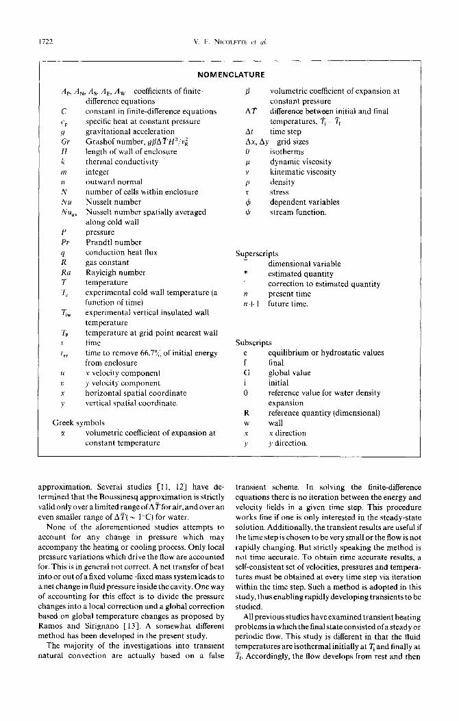
NOMENCLATURE

4, A,, 4 A,, A, coefficients of finite- B volumetric coefficient of expansion at

difference equations constant pressure

C constant in finite-difference equations A’i; difference between initial and final

(‘P specific heat at constant pressure temperatures, T - rf

u gravitational acceleration Af time step

Gr Crashof number, yBAiiH3/vi Ax, Ay grid sizes

H length of wall of enclosure 0 isotherms

k thermal conductivity p dynamic viscosity m integer v kinematic viscosity n outward normal Y density N number of cells within enclosure T stress NU Nusselt number

Nn,, Nusselt number spatially averaged ;

dependent variables stream function.

along cold wall P pressure Pr Prandtl number

: conduction heat flux Superscripts gas constant dimensional variable

Ra Rayleigh number * estimated quantity T temperature correction to estimated quantity 7, experimental cold wall temperature (a n present time

function of time) n + 1 future time.

7;W experimental vertical insulated wall temperature

Tp temperature at grid point nearest wall t time Subscripts

t er time to remove 66.70/, of initial energy e equilibrium or hydrostatic values

from enclosure f final

u Y velocity component G global value

L: y velocity component i initial

Y horizontal spatial coordinate 0 reference value for water density

I’ vertical spatial coordinate. expansion R reference quantity (dimensional)

Greek symbols W wall r volumetric coefficient of expansion at X x direction

constant temperature Y y direction.

approximation. Several studies [Il. 121 have determined that the Boussinesq approximation is strictly valid only over a limited range of AT for air, and over an even smaller range of AT( - 1°C) for water.

None of the aforementioned studies attempts to account for any change in pressure which may

accompany the heating or cooling process. Only local pressure variations which drive the flow are accounted for. This is in general not correct. A net transfer of heat into or out of a fixed volume-fixed mass system leads to a net change in fluid pressure inside the cavity. One way of accounting for this effect is to divide the pressure changes into a local correction and a global correction based on global temperature changes as proposed by Ramos and Sirignano [13]. A somewhat different method has been developed in the present study.

The majority of the investigations into transient natural convection are actually based on a false

transient scheme. In solving the finite-difference equations there is no iteration between the energy and velocity fields in a given time step. This procedure works fine if one is only interested in the steady-state solution. Additionally, the transient results are useful if the time step is chosen to be very small or the flow is not

rapidly changing. But strictly speaking the method is not time accurate. To obtain time accurate results, a self-consistent set of velocities, pressures and temperatures must be obtained at every time step via iteration within the time step. Such a method is adopted in this study, thus enabling rapidly developing transients to be studied.

All previous studies have examined transient heating problems in which the final state consisted ofa steady or periodic flow. This study is different in that the fluid temperatures are isothermal initially at z and finally at T. Accordingly, the flow develops from rest and then

Transient cooling by natural convection in a two-dimensional square enclosure 1723

dies out, thus there is no ambiguity as to the initial or

final flow field. The boundary conditions employed in

this study are also unique : three insulated walls and one

vertical wall cooled via a step change in temperature. Note that the problem of transient heating in an enclosure with similar boundary conditions would yield the same insight into the physics of the flow field.

There are two main aspects ofthis study. First, a self- consistent transient variable-property finite-difference

calculation scheme capable of accounting for changes in global pressure is developed. The results of experiments conducted with air as the working fluid in which one vertical wall is cooled as a function of time and the other walls are insulated are used for validation of the numerical method. Then, this numerical scheme

is employed to simulate the transient laminar natural convection of air and water in square two-dimensional enclosures with one vertical wall cooled via step change

in temperature and the other three walls adiabatic. Spatially averaged time-dependent Nusselt numbers are presented for air filled and water filled enclosures in the range of 10’ < Gr < 10’. Isotherms and streamlines are presented which yield insight into the transient enclosure natural convection phenomena.

PROBLEM STATEMENT AND

GOVERNING EQUATIONS

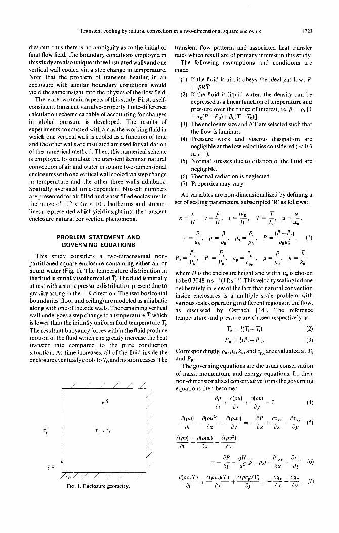
This study considers a two-dimensional non- partitioned square enclosure containing either air or liquid water (Fig. 1). The temperature distribution in

the fluid is initially isothermal at T. The fluid is initially at rest with a static pressure distribution present due to gravity acting in the -j direction. The two horizontal boundaries (floor and ceiling) are modeled as adiabatic along with one of the side walls. The remaining vertical wall undergoes a step change to a temperature Tr which is lower than the initially uniform fluid temperature T. The resultant buoyancy forces within the fluid produce motion of the fluid which can greatly increase the heat transfer rate compared to the pure conduction situation. As time increases, all of the fluid inside the enclosure eventually cools to q, and motion ceases. The

r

,&u i / /’ /’ / /

FIG. 1. Enclosure geometry.

transient flow patterns and associated heat transfer

rates which result are of primary interest in this study.

The following assumptions and conditions are made :

(1)

(2)

(3)

(4)

If the fluid is air, it obeys the ideal gas law: P = ,TRT If the fluid is liquid water, the density can be expressed as a linear function of temperature and pressure over the range of interest, i.e. p = po[l

+%(~-P,)+Bd~-m The enclosure size and Arare selected such that the flow is laminar.

(5)

Pressure work and viscous dissipation are negligible at the low velocities considered (< 0.3 m s-l).

Normal stresses due to dilation of the fluid are negligible.

(6) Thermal radiation is neglected.

(7) Properties may vary.

All variables are non-dimensionalized by defining a set of scaling parameters, subscripted ‘R’ as follows :

where H is the enclosure height and width. uR is chosen to be0.3048 m s- ’ (1 ft s-i). This velocity scalingis done

deliberately in view of the fact that natural convection inside enclosures is a multiple scale problem with various scales operating in different regions in the flow, as discussed by Ostrach [14]. The reference temperature and pressure are chosen respectively as

TR = $(T+ r;) (2)

P, = +((Pi + P,). (3)

Correspondingly, pR, pR, k,, and cpa are evaluated at TR and P,.

The governing equations are the usual conservation of mass, momentum, and energy equations. In their non-dimensionalized conservative forms the governing equations then become :

aP 3PU) I d(P4 _ o z+- dX iiy (4)

a(Pu) + 8(PU2) + 4PU4 __ ~ ~ at ax ay

=-!!+%+ir- (5)

aY

a(P4 + e4 + a(d) at ax ay

ap gH

ay -$p-p._)+%+% (6)

d(PcP*) ( P ; p ah UT) d(PC UT) aqx at ax ay

-3. (7) =-Z ay

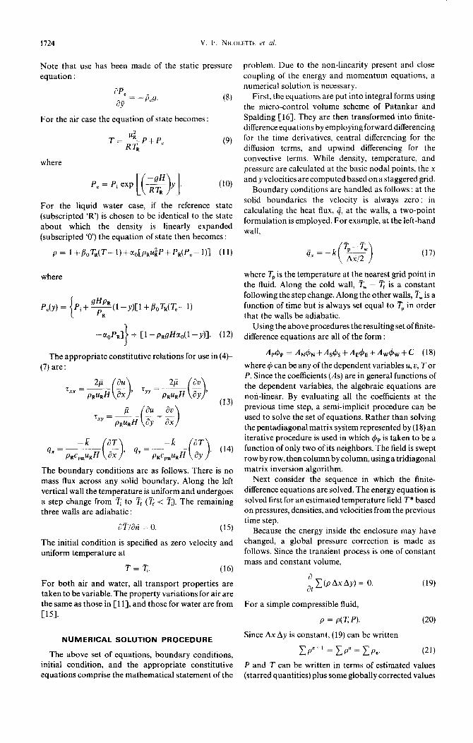
1724 V. I;. NICOLETTE c't ul.

Note that use has been made of the static pressure equation :

f?P 2 = -peg. aj

For the air case the equation of state becomes :

4 T==P+P, (9)

R

where

P, = Pi exp (10)

For the liquid water case, if the reference state (subscripted ‘R’) is chosen to be identical to the state about which the density is linearly expanded (subscripted ‘0’) the equation of state then becomes :

p= ~+P~TR(T-~)+~,[~Ru~P+PR(P,-~)] (11)

where

pJY) = {

pi+ F(l -Y)[l +&T,(T,- 1) R

- a,pR1 I + Cl-pRgH%(l -Y)l. (12)

The appropriate constitutive relations for use in (4)-

(7) are :

Tx.x = 2ji at4 ~ -

0 pRuRH ax ’

p Txy = -

PRURH

3 Tyy = ___

PRURH

au 0 ay’ (13)

) (14)

The boundary conditions are as follows. There is no mass flux across any solid boundary. Along the left vertical wall the temperature is uniform and undergoes a step change from ;i to Tr (T, < T). The remaining three walls are adiabatic :

aTian = 0. (13

The initial condition is specified as zero velocity and uniform temperature at

ii= T. (16)

For both air and water, all transport properties are taken to be variable. The property variations for air are the same as those in [ 111, and those for water are from

Cl51.

NUMERICAL SOLUTION PROCEDURE

The above set of equations, boundary conditions, initial condition, and the appropriate constitutive equations comprise the mathematical statement of the

problem. Due to the non-linearity present and close

coupling of the energy and momentum equations, a numerical solution is necessary.

First, the equations are put into integral forms using the micro-control volume scheme of Patankar and Spalding [16]. They are then transformed into finite- difference equations by employing forward differencing for the time derivatives, central differencing for the diffusion terms, and upwind differencing for the convective terms. While density, temperature, and pressure are calculated at the basic nodal points, the x and y velocities are computed based on a staggered grid.

Boundary conditions are handled as follows : at the solid boundaries the velocity is always zero; in

calculating the heat flux, 4, at the walls, a two-point formulation is employed. For example, at the left-hand wall,

(17)

where Tp is the temperature at the nearest grid point in the fluid. Along the cold wall, Tw = Tr is a constant following the step change. Along the other walls, ??w is a function of time but is always set equal to 5 in order

that the walls be adiabatic. Using the above procedures the resulting set of finite-

difference equations are all of the form :

&#+ = A,~,+A,~,+A,~,+A,~,+C (18) where 4 can be any of the dependent variables u, v, T or P. Since the coefficients (As) are in general functions of the dependent variables, the algebraic equations are non-linear. By evaluating all the coefficients at the previous time step, a semi-implicit procedure can be used to solve the set of equations. Rather than solving the pentadiagonal matrix system represented by (18) an iterative procedure is used in which ~$a is taken to be a function of only two of its neighbors. The field is swept

row by row, then column by column, using a tridiagonal matrix inversion algorithm.

Next consider the sequence in which the finite-

difference equations are solved. The energy equation is solved first for an estimated temperature field T* based on pressures, densities, and velocities from the previous time step.

Because the energy inside the enclosure may have changed, a global pressure correction is made as follows. Since the transient process is one of constant mass and constant volume,

(19)

For a simple compressible fluid,

P = Pm PI.

Since Ax Ay is constant, (19) can be written

c-m

CP n+’ = Cp”= Cpe. (21)

P and T can be written in terms of estimated values (starred quantities) plus some globally corrected values


(primed quantities) as follows :

P = P*+& (22)

T = T*+Tb. (23)

Assume for the moment that Tb is zero, and that the estimated temperature field T* (from the previous time step or iteration) is correct. Using the ideal gas law and substituting (22) and (23) into (21), after some algebra, yields

(24)

Allofthecellpressures are thenequally adjusted via(22)

and (24) to obtain a new globally corrected pressure which conserves mass at constant volume. A similar expression can be derived for the liquid case using the liquid equation ofstate. This differs from the method of Ramos and Sirignano [ 133 in that the global pressure

correction can be immediately estimated without requiring simultaneous global correction of the temperature field.

In situations where there are large changes in pressure inside the enclosure or where fluid properties

are strong functions of pressure, the use of the global pressure correction can greatly affect the results. This is particularly true in liquid filled enclosures where the density is very insensitive to pressure. In such situations a slight change in average fluid temperature results in large pressure changes in order to maintain a constant average density (or constant mass). For water at 20°C and 1 atm,

/?/a g + 5.065 x 10’ Pa “C-l (f 2.78 atm “F-l).

(25)

If the process is one of heating, the subsequent increase in pressure may quickly cause the enclosure to rupture. When the process is a cooling process, the subsequent

decrease in pressure may cause the container to collapse or could theoretically lead to a two-phase liquid-vapor mixture or a liquid in a non-equilibrium state, greatly affecting the heat transfer.

Having obtained estimates of T and P for the given time step, the densities are then calculated from the equation of state and the other properties are updated. Now first estimates of the velocities u* and u* can be made from the momentum equations. Since these estimated velocities will not in general conserve mass locally within each cell, the local pressure field must be corrected to reduce the residual mass terms. Using these locally corrected pressures, new velocities can be

calculated. Iteration proceeds among u*, u*, and P’ until the sum of the squares of the local mass sources is made as small as desired.

In the false transient approach the calculations then proceed to the next time level. This is acceptable if the time step is very small relative to the rate at which the flow field is developing or if one is only interested in steady-state results. However, in general the estimated

values of T, P, p, u and u are not correct since they are based on coefficients involving the previous time level

values. Therefore, in this study, iterations are made

within each time step, taking this newly calculated set of values and feeding it back into the computations. The spatially average Nusselt number along the cold wall is compared from iteration to iteration. When the percent change in Nusselt numbers between consecutive iterations is less than O.l%, a consistent set of 7; P, p, u and u is assumed to have been obtained and the calculations proceed to the next time step. Spatially local Nusselt numbers and r.m.s. Nusselt numbers were also tried as the criterion without any influence on the

results. Eventually a final state is reached in which the velocities are zero and all temperatures equal the cold wall temperature Tp

In the present work a uniform 42 x 42 grid with Ax = Ay was used. A denser grid was experimented with without significant differences in the results [17]. A non-uniform mesh with fewer nodal points could

also have been used [18] but would be slightly more difficult to implement and would require some adjust-

men; of the global pressure correction. A time step of 0.001 < Ai< 0.01 s was used in all numerical simulations.

It may be of interest to note that the numerical procedure described herein is essentially of the same basic type as that of Patankar and Spalding [16]. Notable differences include the introduction of the global pressure correction routine, the self-consistent iterations for both the momentum and energy fields within each time step, and the use of only upwind differencingfor the convection terms. The validity ofthe use of upwind differencing in two-dimensional enclosure problems has been critically examined and

substantiated in [l 1, 18,203.

EXPERIMENTAL SETUP AND PROCEDURE

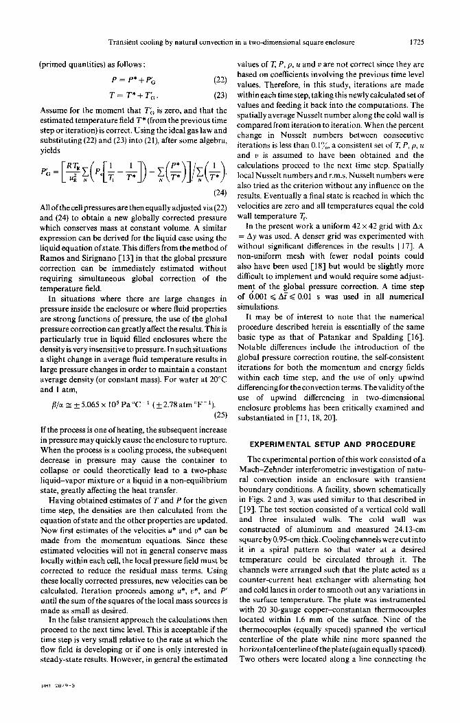
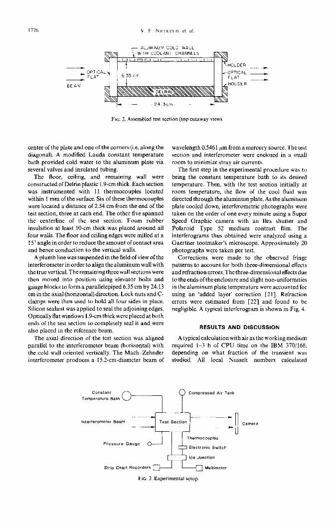
The experimental portion of this work consisted of a Mach-Zehnder interferometric investigation of natural convection inside an enclosure with transient boundary conditions. A facility, shown schematically in Figs. 2 and 3, was used similar to that described in [ 191. The test section consisted of a vertical cold wall and three insulated walls. The cold wall was constructed of aluminum and measured 24.13-cm square by0.95cm thick. Cooling channels were cut into it in a spiral pattern so that water at a desired temperature could be circulated through it. The channels were arranged such that the plate acted as a counter-current heat exchanger with alternating hot and cold lanes in order to smooth out any variations in the surface temperature. The plate was instrumented with 20 30-gauge copper-constantan thermocouples located within 1.6 mm of the surface. Nine of the thermocouples (equally spaced) spanned the vertical centerline of the plate while nine more spanned the horizontal centerline ofthe plate (again equally spaced). Two others were located along a line connecting the

1726

--ALUMINUM COLD WALL

BEAM

WITH COOLANT CHANNELS

HOLDER

OPTICAL FLAT

HOLDER

24 13cm

FIG. 2. Assembled test section (top cutaway view).

center of the plate and one of the corners (i.e. along the diagonal). A modified Lauda constant temperature

bath provided cold water to the aluminum plate via several valves and insulated tubing.

wavelength 0.5461 pm from a mercury source. The test section and interferometer were enclosed in a small room to minimize stray air currents.

The floor, ceiling, and remaining wall were constructed of Delrin plastic 1.9-cm thick. Each section was instrumented with 11 thermocouples located within 1 mm of the surface. Six of these thermocouples were located a distance of 2.54 cm from the end of the

test section, three at each end. The other five spanned the centerline of the test section. Foam rubber insulation at least lo-cm thick was placed around all four walls. The floor and ceiling edges were milled at a 15” angle in order to reduce the amount of contact area

and hence conduction to the vertical walls.

The first step in the experimental procedure was to

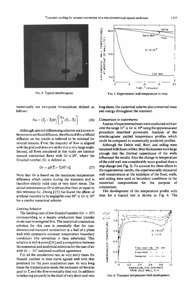
bring the constant temperature bath to its desired temperature. Then, with the test section initially at room temperature, the flow of the cool fluid was directed through the aluminum plate. As the aluminum plate cooled down, interferometric photographs were taken on the order of one every minute using a Super Speed Graphic camera with an Ilex shutter and Polaroid Type 52 medium contrast film. The interferograms thus obtained were analyzed using a Gaertner toolmaker’s microscope. Approximately 20

photographs were taken per test. A plumb line was suspended in the field of view of the

interferometer in order to align the aluminum wall with the true vertical. The remaining three wall sections were then moved into position using elevator bolts and

gauge blocks to form a parallelepiped 6.35 cm by 24.13 cm in the axial (horizontal) direction. Lock nuts and C- clamps were then used to hold all four sides in place. Silicon sealant was applied to seal the adjoining edges. Optically flat windows 1.9-cm thick were placed at both ends of the test section to completely seal it and were also placed in the reference beam.

Corrections were made to the observed fringe

patterns to account for both three-dimensional effects and refraction errors. The three-dimensional effects due

to the ends ofthe enclosure and slight non-uniformities in the aluminum plate temperature were accounted for using an ‘added layer’ correction [21]. Refraction errors were estimated from [22] and found to be negligible. A typical interferogram is shown in Fig. 4.

RESULTS AND DISCUSSION

The axial direction of the test section was aligned A typical calculation with air as the working medium

parallel to the interferometer beam (horizontal) with required l-3 h of CPU time on the IBM 370/168,

the cold wall oriented vertically. The Mach--Zehnder depending on what fraction of the transient was

interferometer produces a 15.2-cm-diameter beam of studied. All local Nusselt numbers calculated

constant Temperature Bath

Compressed Air Tank

Interferometer Seam Test Section Camera -

Electronic Swtch

Ice Junction

Strip Chart Recorders Multimeter

FIG. 3. Experimental setup.


FIG. 4. Typical interferogram.

numerically are two-point formulations defined as long times, the numerical scheme also conserved mass follows: and energy throughout the transient.

Nu = (5- T)H;E(7;-- T)]. (26)

Although upwind differencing schemes are known to be prone to artificial diffusion, the effects ofthis artificial diffusion on the results is believed to be minimal for several reasons. First, the majority of flow is aligned with the grid and does not strike it at a very large angle. Second, all flows simulated in this study are laminar natural convection flows with Gr ,< 107, where the Grashof number, Gr, is defined as

Gr = sp( ;ii’- iJH3/v: (27)

Note that Gr is based on the maximum temperature difference which occurs during the transient and is therefore strictly valid only at very short times. The actual instantaneous Gr is always less than or equal to this reference Gr. Zhong [23] has found the effects of artificial viscosity to be negligible over lo3 < Gr < lo6 for a similar numerical scheme.

Limiting behavior The limiting case of low Grashof number (Gr = 103)

corresponding to a mainly conduction heat transfer mode was investigated first. The analytical conduction solution for this case is essentially that for one- dimensional transient conduction in a half of a plane wall with symmetric constant temperature boundary conditions (the centerline is then adiabatic). This solution is well-known [24] and a comparison between the numerical and analytical solutions for the case of air with Gr = lo3 indicated excellent agreement.

For all the simulations run, at very early times the Nusselt number vs time curve agreed well with that predicted for the pure conduction case. At very long times the temperatures inside the enclosure all became qua1 to T; and the flow eventually died out. In addition to behaving properly in the limit of very short and very

Gr=13x105

0 5 IO 15 20

TIME.7 (minutes)

FIG. 5. Experimental wall temperature vs time.

Comparison to experiments Aseries ofexperimental tests wereconducted with air

over the range lo5 Q Gr < lo6 using the apparatus and procedure described previously. Analysis of the interferograms yielded temperature profiles which could be compared to numerically predicted profiles.

Although the Delrin wall, floor, and ceiling were insulated with foam rubber, their thicknesses were large enough that the thermal capacitance of the walls influenced the results. Also the change in temperature of the cold wall was considerably more gradual than a step change (see Fig. 5). To account for these effects in the experimental results, the experimentally measured wall temperatures at the midplane of the floor, walls, and ceiling were used as boundary conditions in the numerical computations for the purpose of comparison.

The development of the temperature profile with time for a typical test is shown in Fig. 6. The

Exper,ment o a . Numerical ----

, 0 0.2 0.4 0.6 0.8 1.0

DIMENSIONLESS DISTANCE FROM COLD WALL, i/H

FIG. 6. Transient temperature field development.

1728 V. t-. NI(.OLITTE 01 ul

Gr =B x IO5

Time = 305 set

y LocatIon H/4 Hl2 3H/4

Experiment o a a

Numerical -- - --- 1

u 0’ J

0 0.2 0.4 06 08 IO

DIMENSIONLESS DISTANCE FROM COLD WALL, F/H

FIG. 7. Temperature profiles throughout enclosure.

temperature gradients near the wall increase with time while the core temperature decreases with time in both the numerical and experimental results as expected. Note that during this portion of the transient the cold wall temperature is decreasing with time. Figure 7 presents temperature profiles at heights of H/4, H/2, and 3H/4 at 305 s in the test with Gr = 8 x 105. The

resulting agreement between experimentally measured and numerically predicted profiles in Figs. 6 and 7 is considered good with the experimental data indicating slightly steeper profiles at both walls and a slightly higher average core temperature than the calculated values. Note that there is very little temperature variation outside of the boundary layers in the core region. The experimental error is greatest in the core region where the change in fringe shift is quite gradual. Near the walls the error in reading the interferogram is smaller (- 3%) due to the more rapid change in fringe shift and thus greater accuracy is expected.

There are two plausible explanations for the sharper slopes in the experimental temperature profiles. First, if there is some artificial diffusion in the numerical scheme, it would tend to reduce the sharp temperature gradient near the walls predicted numerically. However, the amount of artificial diffusion present in the calculations is believed to be insignificant as discussed previously. The more probable cause for the

1 6 25 A,r Gr= IO5 AT = 10°C

T R ‘300K

PR = 101 3 kPa

~ Numertcal

01 I 0 20 40 60 80

DIMENSIONLESS TIME, f FIG. 8. Nusselt number vs time: Gr = 105.

All Gr = IO6

= 10°C = 300 K

= 101 3 kPa

~ Numer,cal -,

,;!ij

---_-________ j 01’ 1 d

0 IO 20 30 40 50 60 70 80 90

DIMENSIONLESS TIME.1

FIG. 9. Nusselt number vs time : Gr = lo6

sharper slopes in the experimental results is thought to

be the presence of three-dimensional effects. The optical flats at the test section ends heat up the fluid and cause a weak flow in the longitudinal direction. This results in an enhanced flow of relatively warmer fluid near the middle of the test section and hence a larger heat transfer rate at the cold wall.

Numerical simulation of airjilled enclosures Numerical simulations of the two-dimensional

transient laminar natural convection of air inside square enclosures were conducted for lo3 < Gr < lo’, AT = 10°C and 100°C. In these simulations, the left- hand wall was subjected to a step-change in

temperature (to some lower value) while the three remaining walls were made adiabatic. The fluid was initially at rest at temperature T.

Figure 8 presents the average cold wall Nusselt number vs timeforthecase of Gr = 105,A’i‘ = lO”C.At early times, the heat transfer is due mainly to pure conduction (location 1). During the transition from a conduction to a convection dominated heat transfer mode, the Nusselt number curve passes through a minimum (location 2). This minimum in heat transfer rate corresponds to a maximum in the thermal boundary-layer thickness as predicted analytically by Siegel [25] and as observed experimentally by Goldstein and Eckert [26] for transient laminar free convection from a vertical flat plate. The average Nusselt number then increases slightly and levels off for a short period of time. During this time the presence of the right-hand wall on the heat transfer rate is just beginning to be felt. This is shown by the fact that the Nusselt number plateau (location 3) in Fig. 8 is only 5% smaller than the steady-state solution predicted by Chan and Tien [27] for a three-walled cavity exposed to an infinite amount of ambient fluid. Since in the transient case under consideration the average temperature difference between the cold wall and fluid decreases with time, so does the driving force and the average Nusselt number.

The results of the numerical simulation of air with Gr = lo6 and AT = 10°C are presented in Fig. 9. Again the average Nusselt number agrees initially with the analytical conduction solution (location 1) for short


e (b)t =4.9 ’

2 s I!

s 2 0

0 0

d 0

e (c)t=9.9 JI 8

(d)l=l4.8 ‘+

;&gg ;HH (e) t =18.1

JI e (f)t =26.3 ‘!’

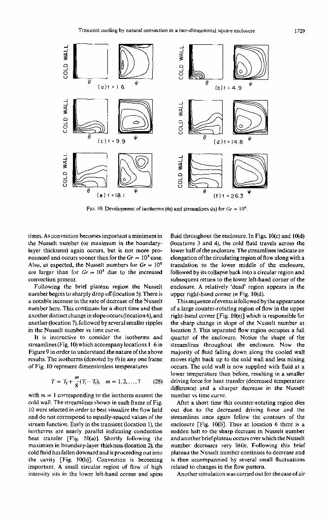
FIG. 10. Development of isotherms (0s) and streamlines I(Is) for Gr = 106.

times. As convection becomes important a minimum in the Nusselt number (or maximum in the boundary- layer thickness) again occurs, but is not more pro- nounced and occurs sooner than for the Gr = lo5 case. Also, as expected, the Nusselt numbers for Gr = lo6 are larger than for Gr = 10’ due to the increased convection present.

Following the brief plateau region the Nusselt number begins to sharply drop off (location 5). There is a notable increase in the rate of decrease of the Nusselt number here. This continues for a short time and then another distinct change in slope occurs (location 6), and another (location 7), followed by several smaller ripples in the Nusselt number vs time curve.

It is instructive to consider the isotherms and streamlines (Fig. 10) which accompany locations l-6 in Figure 9 in order to understand the nature of the above results. The isotherms (denoted by 0) in any one frame of Fig. 10 represent dimensionless temperatures

T= T,++q), m= 1,2 ,..., 7 (28)

with m = 1 corresponding to the isotherm nearest the cold wall. The streamlines shown in each frame of Fig. 10 were selected in order to best visualize the flow field and do not correspond to equally-spaced values of the stream function. Early in the transient (location l), the isotherms are nearly parallel indicating conduction heat transfer [Fig. IO(a)]. Shortly following the maximum in boundary-layer thickness (location 2), the cold fluid has fallen downard and is proceeding out into the cavity [Fig. 10(b)]. Convection is becoming important. A small circular region of flow of high intensity sits in the lower left-hand corner and spins

fluid throughout the enclosure. In Figs. 10(c) and 10(d) (locations 3 and 4), the cold fluid travels across the lower half of the enclosure. The streamlines indicate an elongation of the circulating region of flow along with a translation to the lower middle of the enclosure, followed by its collapse back into a circular region and subsequent return to the lower left-hand corner of the enclosure. A relatively ‘dead’ region appears in the upper right-hand corner in Fig. 10(d).

This sequence ofevents is followed by the appearance of a large counter-rotating region of flow in the upper right-hand corner [Fig. 10(e)] which is responsible for the sharp change in slope of the Nusselt number at location 5. This separated flow region occupies a full quarter of the enclosure. Notice the shape of the streamlines throughout the enclosure. Now the majority of fluid falling down along the cooled wall moves right back up to the cold wall and less mixing occurs. The cold wall is now supplied with fluid at a lower temperature than bkfore, resulting in a smaller driving force for heat transfer (decreased temperature difference) and a sharper decrease in the Nusselt number vs time curve.

After a short time this counter-rotating region dies out due to the decreased driving force and the streamlines once again follow the contours of the enclosure [Fig. lo(f)]. Thus at location 6 there is a sudden halt to the sharp decrease in Nusselt number and another briefplateau occurs over which the Nusselt number decreases very little. Following this brief plateau the Nusselt number continues to decrease and is then accompannied by several small fluctuations related to changes in the flow pattern.

Another simulation was carried out for the case of air

1730 V. F. NICOLETTE CI d.

/ I / --1

WATER Gr q IO’ TR = 493 K

ai=l’c PR = 9 544 MPa

I NUKlerlCOl J

---- Pure conduction

\ ----_ ----~__-_______ 0 I I I I I I I

0 1x102 2 3 4 5 6 7 8

DIMENSIONLESS TIME, t

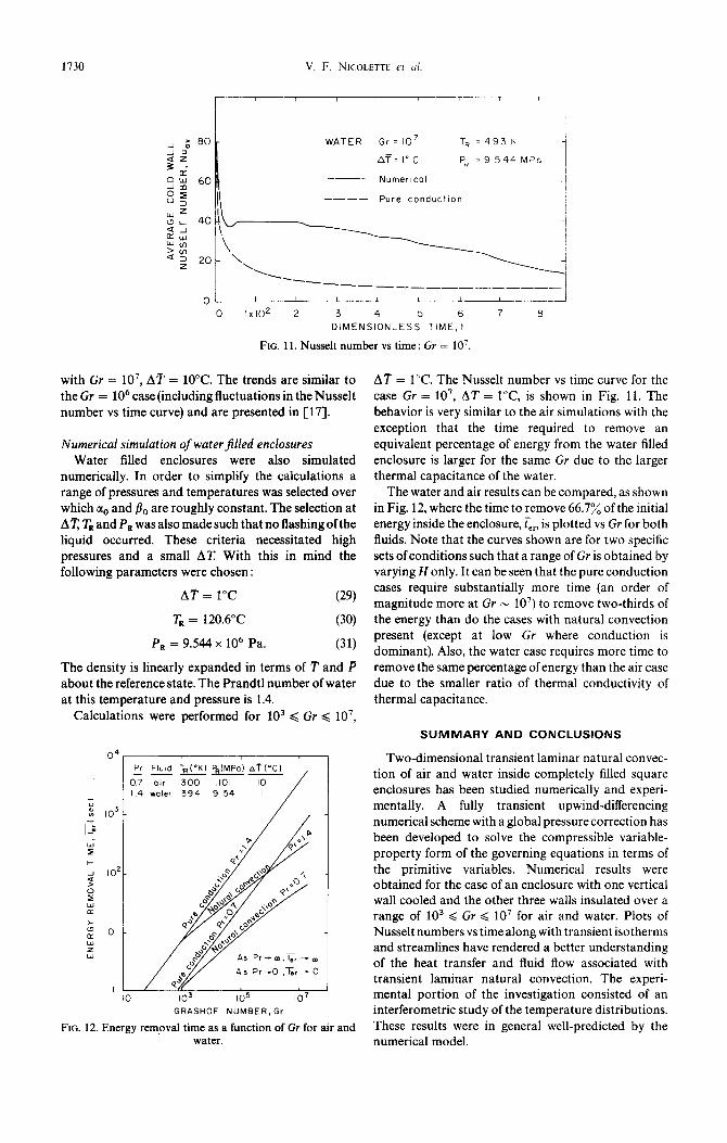
FIG. 11. Nusselt number vs time : Gr = 10’.

with Gr = lo’, AT = 10°C. The trends are similar to the Gr = lo6 case (including fluctuations in the Nusselt number vs time curve) and are presented in [ 171.

Numerical simulation of waterjlled enclosures Water filled enclosures were also simulated

numerically. In order to simplify the calculations a range of pressures and temperatures was selected over which cl0 and Do are roughly constant. The selection at AT TR and P, was also made such that no flashing of the liquid occurred. These criteria necessitated high pressures and a small A5? With this in mind the following parameters were chosen :

AT = 1°C (29)

TR = 120.6”C (30)

P, = 9.544 x lo6 Pa. (31)

The density is linearly expanded in terms of F and P about the reference state. The Prandtl number of water at this temperature and pressure is 1.4.

Calculations were performed for lo3 ,< Gr < IO’,

Pr FluId TRIoK) &.(MPal aT(‘C) -- 07 01r 1 300 ,101

I4 water 394 9 54

I I

A5 Pr-0 ,x,-o

105 IO’

GRASHOF NUMBER,Gr

FIG. 12. Energy removal time as a function of Gr for air and water.

AT = 1°C. The Nusselt number vs time curve for the case Gr = lo’, AT = l”C, is shown in Fig. 11. The behavior is very similar to the air simulations with the exception that the time required to remove an equivalent percentage of energy from the water filled enclosure is larger for the same Gr due to the larger thermal capacitance of the water.

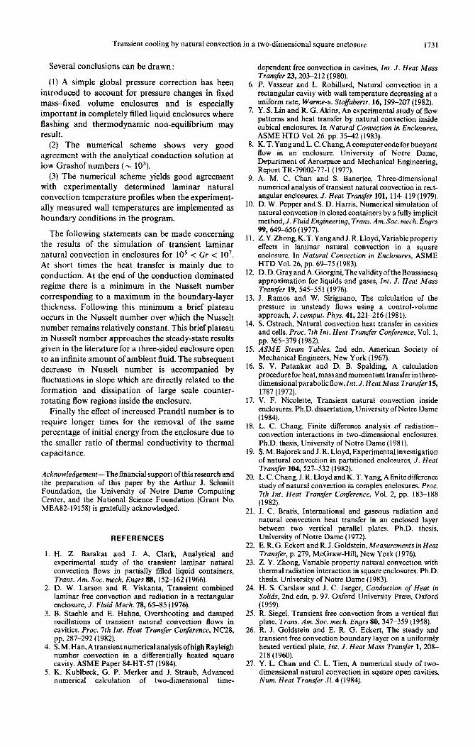
The water and air results can be compared, as shown in Fig. 12, where the time to remove 66.7% of the initial energy inside the enclosure, Fe, is plotted vs Gr for both fluids. Note that the curves shown are for two specific sets of conditions such that a range of Gr is obtained by varying H only. It can be seen that the pure conduction cases require substantially more time (an order of magnitude more at Gr - 10’) to remove two-thirds of the energy than do the cases with natural convection present (except at low Gr where conduction is dominant). Also, the water case requires more time to remove the same percentage of energy than the air case due to the smaller ratio of thermal conductivity of thermal capacitance.

SUMMARY AND CONCLUSIONS

Two-dimensional transient laminar natural convection of air and water inside completely filled square enclosures has been studied numerically and experimentally. A fully transient upwind-differencing numerical scheme with a global pressurecorrection has been developed to solve the compressible variableproperty form of the governing equations in terms of the primitive variables. Numerical results were obtained for the case of an enclosure with one vertical wall cooled and the other three walls insulated over a range of lo3 < Gr < 10’ for air and water. Plots of Nusselt numbers vs time along with transient isotherms and streamlines have rendered a better understanding of the heat transfer and fluid flow associated with transient laminar natural convection. The experimental portion of the investigation consisted of an interferometric study of the temperature distributions.

These results were in general well-predicted by the numerical model.


Several conclusions can be drawn :

(I) A simple global pressure correction has been introduced to account for pressure changes in fixed mass-fixed volume enclosures and is especially important in completely filled liquid enclosures where Bashing and thermodynamic non-equilibrium may result.

(2) The numerical scheme shows very good agreement with the analytical conduction solution at low Grashof numbers (_ 103).

(3) The numerical scheme yields good agreement with experimentally determined laminar natural convection temperature profiles when the experimentally measured wall temperatures are implemented as boundary conditions in the program.

The following statements can be made concerning the results of the simulation of transient laminar natural convection in enclosures for 10’ < Gr < 10’. At short times the heat transfer is mainly due to conduction. At the end of the conduction dominated regime there is a minimum in the Nusselt number corresponding to a maximum in the boundary-layer thickness. Following this minimum a brief plateau occurs in the Nusselt number over which the Nusselt number remains relatively constant. This brief plateau in Nusselt number approaches the steady-state results given in the literature for a three-sided enclosure open to an infinite amount of ambient fluid. The subsequent decrease in Nusselt number is accompanied by fluctuations in slope which are directly related to the formation and dissipation of large scale counter- rotating flow regions inside the enclosure.

Finally the effect of increased Prandtl number is to require longer times for the removal of the same percentage of initial energy from the enclosure due to the smaller ratio of thermal conductivity to thermal capacitance.

Ack~owiedge~ent-The financial support ofthis research and the preparation of this paper by the Arthur J. Schmitt Foundation, the University of Notre Dame Computing Center, and the National Science Foundation (Grant No. MEA82-19158) is gratefully acknowledged.

REFERENCES

1. H. 2. Barakat and 1. A. Clark, Analytical and experimental study of the transient laminar natural convection flows in partially filled liquid containers, Trans. Am. Sot. mech. Engrs 88, 152-162 (1966).

2. D. W. Larson and R. Viskanta, Transient combined laminar free convection and radiation in a rectangular enclosure, J. Fluid Me&. 7%, 65-85 (1976).

3. B. Staehle and E. Hahne, Overshooting and damped oscillations of transient natural convection flows in cavities. Proc. 7th Int. Heat Transfer Conference, NC28, pp. 287-292 (1982).

4. S. M. Han, A transient numerical analysis ofhigh Ravleigh number convection in a differentially heated square cavitv. ASME Paoer 84HT-57 11984).

5. K. Keblbeck, G.‘P. Merker and J.‘Straub, Advanced numerical calculation of two-dimensional time-

6.

7.

8.

9.

10.

11.

12.

13.

14,

1.5

16.

17.

18.

19.

20.

21.

22.

23.

24.

25.

26.

27.

dependent free convection in cavities, Int. J. Heat Mass Transfer 23,203-212 (1980). P. Vasseur and L. Robillard, Natural convection in a rectangular cavity with wall temperature decreasing at a uniform rate, Warme-u. Sto~abertr. 16, 199-207 (1982). Y. S. Lin and R. G. Akins, An experimental study of flow patterns and heat transfer by natural convection inside cubical enclosures. In Natural Convection in Enclosures, ASME HTD Vol. 26, pp. 3542 (1983). K. T. Yang and L. C. Chang, A computer code for buoyant flow in an enclosure. University of Notre Dame, Department of Aerospace and Mechanical En~nee~ng, Report TR-79002-77-l (1977). A. M. C. Chan and S. Banerjee, Three-dimensional numerical analysis of transient natural convection in rectangular enclosures, J. Heat Transfa 101, 114-119 (1979). D. W. Pepper and S. D. Harris, Numerical simulation of natural convection in closed containers by a fully implicit method,J. Fluid ~ngjneer~ng, Trans. Am. Sot. mech. Engrs QQ,649-656 (1977). Z.Y.Zhong,K.T. Yangand J.R.Lloyd,Variableproperty effects in laminar natural convection in a square enclosure. In Natural Convection in Enclosures, ASME HTD Vol. 26, pp. 69-75 (1983). D. D. Grav and A. Gioreini.The validitv ofthe Boussinesa approximation for liquids and gases, fnt. J. Heat Mass Trans~r 19, 545-551 (1976). I. Ramos and W. Sirignano, The calculation of the pressure in unsteady flows using a control-volume approach, J. comput. Phys. 41,221-216 (1981). S. Ostrach, Natural convection heat transfer in cavities and cells. Proc. 7th Int. Heat Transfer Conference, Vol. 1, pp. 365-379 (1982). ASME Steam Tabfes, 2nd edn. American Society of Mechanical Engineers, New York (1967). S. V. Patankar and D. B. Spalding, A calculation procedure for heat, mass and momentum transfer in three- dimensional parabolic flow, Znt. J. Heat Mass Transfer 15, 1787 (1972). V. F. Nicolette, Transient natural convection inside enclosures. Ph.D. dissertation, University of Notre Dame (1984). L. C. Chang, Finite difference analysis of radiation- convection interactions in two-dimensional enclosures. Ph.D. thesis, University of Notre Dame (1981). S. M. Bajorek and J. R. Lloyd, Experimental investigation of natural convection in partitioned enclosures, J. Heat Transfer 104,527-532 (1982). L.C. Chang, J. R. Lloyd and K. T. Yang, A finitedifferen~ study of natural convection in complex enclosures. PTUC. 7th Int. Heat Transfer Conference, Vol. 2, pp. 183-188 (1982). J. C. Bratis, International and gaseous radiation and natural convection heat transfer in an enclosed layer between two vertical parallel plates. Ph.D. thesis, University of Notre Dame (1972). E. R. G. Eckert and R. J. Goldstein, Mea~reme~ts in Heat Trader, p. 279. M~raw-Hill, New York (1976). Z. Y. Zhong, Variable property natural convection with thermal radiation interaction in square enclosures. Ph.D. thesis, University of Notre Dame (1983). H. S. Carslaw and J. C. Jaeger, Conduction of Heat in Solids, 2nd edn, p. 97. Oxford University Press, Oxford (1959). R. Siegel, Transient free convection from a vertical Rat plate, Trans. Am. Sot. mech. Enars 80.347-359 (19581. k. J. Goldstein and E. R. G. Eckert, The steady and transient free convection boundary layer on a uniformly heated vertical plate, Int. J. Heat Mass Transfer 1, 208- 218 (1960). Y. L. Chan and C. L. Tien, A numerical study of two- dimensional natural convection in square open cavities, Num. Heat Transfer Jl. 4 (1984).

1732 v. F YI(‘oLETTt- C’f tri

REFROIDISSEMENT VARIABLE PAR CONVECTION NATURELLE DANS UNE CAVITE CARREE BIDIMENSIONNELLE

R&m&On conduit une recherche numirique et experimentale sur la convection naturelle variable, bidimensionnelle, monophasique dans une cavite carrte entierement remplie, avec une paroi verticale refroidie soumise g un changement en echelon de temperature) et les trois autres parois isolantes. Un schema semi- implicite entiirement variable avec une correction de pression globale est utili& pour la simulation numerique d’air et d’eau dans le domaine lo5 < Gr < 10’. Experimentalement, un interferometre Mach- Zehnder est utilise pour obtenir des distributions variables de temperature dans la caviti qui sont comparees aux resultats numeriques. On trouve un bon accord entre les donnbes experimentales et les previsions

numtriques.

INSTATIONARER KUHLVORGANG BE1 NATURLICHER KONVEKTION IN EINEM ZWEIDIMENSIONALEN QUADRATISCHEN GEBIET

Zusammenfassung-Es wurde eine numerische und experimentelle Untersuchung der zweidimensionalen instationlren natiirlichen Konvektion von einphasigen Fluiden innerhalb eines vollstlndig gefiillten quadratischen Gebietes durchgefiihrt. Eine senkrechte Wand war gekiihlt, wobei die Temperatur sprunghaft abgesenkt wurde. Die anderen drei Wande waren warmegedammt. Ein vollstiindig instationares semi- implizites Vorwlrts-Differenzenverfahren mit einer umfassenden Druckkorrektur wurde fur die numerische Simulation fur Luft und Wasser im Bereich von lo5 < Gr < 10’ angewandt. Ein Mach-Zehnder Interferometer wurde verwendet, urn die zeitlichen Temperaturverteilungen im Gebiet als Vergleich zu den Rechenergebnissen experimentell zu ermitteln. Es wurde eine gute Ubereinstimmung zwischen den

Versuchsdaten und den numerischen Vorausberechnungen gefunden.

HECTAHMOHAPHOE OXJIA)KflEHkiE HPM ECTECTBEHHOH KOHBEKHHM B 3AMKHYTOn IIOJIOCTM KBAAPATHOFO CEYEHMFI

hHOTaUHn-npOBeAeH0 YACJIeHHOe M 3KCnepIiMeHTaJIbHOe HCCJleAOBaHAe AByMepHd HeCTaUPiOHapHOii

eCTeCTBeHHOii KOHBeKUUU OAHO@a3HbIX XWiAKOCTeii, IIOMemeHHbIX B UeJIIlKOM 3anOJIHeHHylO eMKOCTb

KBaApaTHOrO Ce'ieHHR, OAHa BepTHKaAbHaK CTeHKa KOTOpOfi 0XJIa;lcAaeTCK (CTytIeHYaTOe H3MeHeHAe

TeMnepaTypbI), a Tpll ApyrHX-aAHa6aTWieCKHe. &In 'IBCJIeHHOTO MOAeJILipOBaHWI Te'ieHUIl B AEiana-

3oHe lo5 < Gr < 1O'npeMeHnnacb HecTauaoHapHan nony-HeaBHaR npoTuBoTorHaa pa3HocTHaxcxeMac

rJIO6aJIbHoti KOppeKU~e~AaBAeH~~.B3KCnep~MeHTaXAA~~OAy~eHARHeCTaU~OHapHbIXpaC~peAeAeHA~

TeMnepaTypbI B 3aMKHyTOii nOJIOCTH ACnOJIb30BaJICR HHTep+pOMeTp Maxa-Hannepa. AaHHbIe 3KCne-

PWMeHTa CpaBHHBanHCb C 'illCJleHHbIMA pe3yJIbTaTaMH. HafineHo XOpOIUee COrJIaCEie MemAy 3KCnepW

Transient cooling by natural convection in a two-dimensional square enclosure

Documents