Trajectory tracking of mobile robots in dynamic environments - a linear algebra approach

Robotica (2009) volume 27, pp. 981–997. © Cambridge University Press 2009doi:10.1017/S0263574709005402

Trajectory tracking of mobile robots in dynamicenvironments—a linear algebra approachAndres Rosales∗, Gustavo Scaglia, Vicente Mut andFernando di SciascioInstituto de Automatica (INAUT), Universidad Nacional de San Juan, Av. Libertador San Martın 1109 (oeste) – J5400ARL,San Juan, Argentina.

(Received in Final Form: January 26, 2008. First published online: February 26, 2009)

SUMMARYA new approach for navigation of mobile robots in dynamicenvironments by using Linear Algebra Theory, NumericalMethods, and a modification of the Force Field Methodis presented in this paper. The controller design is basedon the dynamic model of a unicycle-like nonholonomicmobile robot. Previous studies very often ignore thedynamics of mobile robots and suffer from algorithmicsingularities. Simulation and experimentation results confirmthe feasibility and the effectiveness of the proposed controllerand the advantages of the dynamic model use. By using thisnew strategy, the robot is able to adapt its behavior at theavailable knowing level and it can navigate in a safe way,minimizing the tracking error.

KEYWORDS: Collision avoidance; Dynamic model; Forcefield method; Linear algebra; Mobile robot; Trajectorytracking.

1. IntroductionMobile robots navigation problem in real environments hasbeen an interesting area for researches in the last years.There are numerous papers focused on solving this matterin different ways. The challenge is to obtain a controllerto navigate autonomously in environments with static anddynamic obstacles, especially when these objects have anunknown movement. But, to obtain satisfactory results duringits assigned mission, a mobile robot needs to follow, in anexact way, a previously established path or trajectory. If theaforementioned characteristic is achieved with a minimumof error, the mobile robot will be able to avoid collisions andcome back to its path or trajectory with a better performance.Traditional approaches as path planning methods are slowto be applied in real time44 and due to this drawback, newtechniques are necessary.

When a mobile robot navigates in a real environment,unexpected static and dynamic obstacles are a big problemfor a suitable autonomous navigation, hence a good reactivebehavior is a reasonable way to avoid collisions, in this case,the important thing is not the optimality but the safety ofthe robot’s movement. On the other hand, if obstacles have

* Corresponding author. E-mail: [email protected]

full known movements (or positions), an optimal motioncan be generated by using space–time planning. In severalapplications, it can perform a localization of the environmentby means of the construction of a work-area map from robotsensors. These maps are useful to find the free collisions pathwith static objects as walls or closed doors, etc. However, formobile objects (e.g. humans, other robots, etc.), it is not aneasy task, because the robot must draw dynamic maps withalternative paths or trajectories for the avoidance and hold adesired distance as regards the obstacle. The robot requiresa quick dynamic reaction to avoid collisions with all objectsinstead of depending on static (or dynamic) maps, which areupdated very slowly.

Global methods (e.g. path planning algorithms) calculatea whole path to the goal from the actual robot position.24 Ifthere are mobile obstacles, a common technique entails toadd another dimension—the time—at the space state, so thatthe dynamic problem is reduced to a static one.14 However,even when global methods supply optimal solutions, theirgreater disadvantage is assuming a full knowledge of theenvironment. In practical applications, these techniques areusually combined with local methods to avoid unexpectedobstacles.2,19,20,39,42 Local methods, also called reactivemethods, only generate the next control signal; they just usea closer part of the environment and update the world modelin accordance with the actual observation of the sensors.Most development techniques, such as Dynamic WindowApproach,12 Curvature Velocity Approach,30 Curvature PathApproach,41 and Inevitable Collision States Concept,13,34

depend on a full knowledge of the environment to get agood performance.

Some researches have developed a great variety of methodsbased on the potential field concept. Laplace equation wasused in ref. [5] to avoid local minimums. To overcomedeficiencies in the potential field method, Vector FieldHistogram (VFH)2 was developed, it looks for spaces inpolar histograms locally built. To protect the robot againstcollisions, a repulsive field localized in its neighborhood waspresented in ref. [28]. Later, the VFH+47 and the VFH∗46

methods were developed. A fractional potential method wasdeveloped in ref. [16], which define attractive and repulsivepotentials, taking into account the relative position andvelocity of a robot as regards the obstacles and objectives.Wang et al.49 introduced a variable speed force field methodfor the multirobot collaboration.

982 Trajectory tracking of mobile robots

The use of path tracking in a navigation system isjustified in structured workspaces as well as in partiallystructured workspaces in which unexpected obstacles canbe found during navigation. In the first case, the referencetrajectory can be set from a global trajectory planner. Inthe second case, algorithms used to avoid obstacles re-planthe trajectory in order to avoid a collision; then, a newreference trajectory, which must be followed by the robot,is generated. Furthermore, there are algorithms that expressthe reference trajectory of the mobile robot as a functionof a descriptor called r7 or s, called “virtual time,”25 whosederivative is a function of the tracking error and the time t . Forexample, if the tracking error is large, the reference trajectoryshould wait for the mobile robot; on the other hand, if thetracking error is small, then the reference trajectory must tendto the original trajectory calculated by the global planner.Accordingly, the module of trajectory tracking will use theoriginal path or the online re-calculated path as reference toobtain the smallest error when the mobile robot follows thepath.32 Consequently, the path tracking is always importantindependently from whether the reference trajectory has beengenerated by a global trajectory planner or a local one.

Several studies have been published regarding the design ofcontrollers to guide mobile robots during trajectory tracking.Some of the controllers designed so far are based onlyon the kinematics of the mobile robot, like the controllerspresented in refs. [37, 38]. Other types of tracking controllersbased on robot dynamics are presented by Liu et al.26 andDong & Guo,9 but the results shown are just based onsimulations. In Hwang & Chang17 a decentralized controlby using a mixed robust control is presented. Shuli40

introduces a controller based on the error model of Kanayamaet al.21 As a result, instead of just one controller, twoare handed, which are used depending on whether theangular velocity is null or not. In ref. [50] adaptive controlvia Lyapunov techniques is developed. Kim22 proposes areceding horizon tracking control for time-varying linearsystems with constraints both on the control signal and on thetracking error, based on the minimization of a functional forfinite-time costs. Besides, Linear Matrix Inequalities (LMI)are used in order to synthesize the controller. Fukao et al.15

presents the design of an adaptive tracking controller for thedynamic model based on torque with unknown parameters,but only simulation results are presented. Yang & Kim51

proposed a robust tracking controller for nonholonomicwheeled mobile robots using sliding mode. In ref. [10]fuzzy logic and neural network control approaches wereused to deal with the disturbances and dynamic uncertainties.Yang et al.52 introduced an intelligent predictive controlapproach for the path tracking problem. In ref. [11], thebackstepping technique was used to design the adaptive androbust controller for the nonholonomic system. Kanayamaet al.21 developed smooth static time invariant state feedbackfor a velocity-controlled mobile robot with nonholonomicconstraint. Most papers about the trajectory tracking haveinteresting solutions for this theme, but they do not presentexperimental results or do not work in real environments withthe presence of different kinds of obstacles.

The trajectory tracking for mobile robots is char-acteristically a nonlinear problem. Diverse model-based

classic techniques, which propose controllers with a zero-error tracking, have been applied to solve this problem.However, these classic approaches involve an onlinematrix inversion,23,48 which represents a drawback inthe implementation of the aforementioned methods. Inthis paper, the proposed algorithm leads the trajectorytracking errors to zero, and it does not involve onlinematrix inversion problems. Most of the surveys do notpresent a final expression for the control signals oftheir controllers,18,27,45,50 because the computation of thesecontrol variables must be made by using demandingcomputer operations. On the other hand, some currentstraightforward methods present just simulations).9,26,53 Inthis paper, the design of the proposed control law by usingLinear Algebra tools is intuitive, and furthermore the finalexpression for the control signals, which will be directlyimplemented on the mobile robot, is presented.

The aim of this paper is to use the linear algebra theoryand numerical methods to compute control actions, so that,the mobile robot achieves a position (x, y), with a pre-established orientation ψ at each sample time (kTo) withoutcollisions during its navigation. To achieve this objective, ina nonholonomic vehicle, two control variables are available:the linear velocity u and the rotational velocity ω. Theproposed controller, based on the dynamic model of anonholonomic mobile robot, computes the optimal controlaction (according to least squares43), which allows themobile robot to go from the actual state to the desired one.Furthermore, this paper proposes working with the dynamicmodel of the mobile robot, because this characteristic allowsthe controller to face up to sudden velocity changes and toimprove the performance of the system.4 This linear algebrabased approach has been tested on other works such as workby Rosales et al.35 and Scaglia et al.36–38

In this work, simulations and experimental results havebeen applied to a PIONEER 3DX mobile robot. The efficacyand feasibility are then demonstrated in a practical sensethrough a set of experiments where the speed-range is similarto the one reported in other papers about trajectory trackingusing laboratory equipment.31

The paper is organized as follows: Section 2 describes thedynamic model of the mobile robot. Section 3 presents themethodology to compute the linear algebra based controller.Modified force field method is described in Section 4.Section 5 presents simulations and experimental resultsusing the proposed controller on a PIONEER 3DX mobilerobot. Conclusions are detailed at Section 6. Finally, theAppendix introduces the stability analysis of the proposedcontrollers.

2. Dynamic Model of A Mobile RobotTo perform tasks with requirements of high speed and/ortransport of heavy loads, it is very important to consider thedynamics of the mobile robot, because such tasks exert verylarge external forces on the robot and they will inevitablyinfluence its path and direction, hence, a kinematic model isnot sufficient. Dynamic characteristics of the robot such asmass and inertia center change if the robot is loaded. Previousstudies very often ignore the dynamics of mobile robots and

Trajectory tracking of mobile robots 983

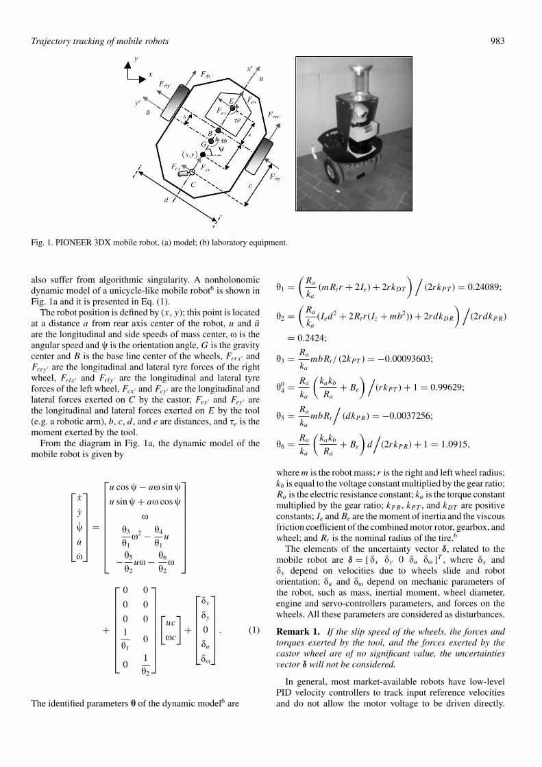
Fig. 1. PIONEER 3DX mobile robot, (a) model; (b) laboratory equipment.

also suffer from algorithmic singularity. A nonholonomicdynamic model of a unicycle-like mobile robot6 is shown inFig. 1a and it is presented in Eq. (1).

The robot position is defined by (x, y); this point is locatedat a distance a from rear axis center of the robot, u and u

are the longitudinal and side speeds of mass center, ω is theangular speed and ψ is the orientation angle, G is the gravitycenter and B is the base line center of the wheels, Frrx ′ andFrry ′ are the longitudinal and lateral tyre forces of the rightwheel, Frlx ′ and Frly ′ are the longitudinal and lateral tyreforces of the left wheel, Fcx ′ and Fcy ′ are the longitudinal andlateral forces exerted on C by the castor, Fex ′ and Fey ′ arethe longitudinal and lateral forces exerted on E by the tool(e.g. a robotic arm), b, c, d, and e are distances, and τe is themoment exerted by the tool.

From the diagram in Fig. 1a, the dynamic model of themobile robot is given by

⎡⎢⎢⎢⎢⎢⎢⎣

x

y

ψ

u

ω

⎤⎥⎥⎥⎥⎥⎥⎦ =

⎡⎢⎢⎢⎢⎢⎢⎢⎢⎢⎢⎣

u cosψ− aω sinψ

u sinψ+ aω cosψ

ω

θ3

θ1ω2 − θ4

θ1u

−θ5

θ2uω− θ6

θ2ω

⎤⎥⎥⎥⎥⎥⎥⎥⎥⎥⎥⎦

+

⎡⎢⎢⎢⎢⎢⎢⎢⎢⎢⎣

0 0

0 0

0 0

1

θ10

01

θ2

⎤⎥⎥⎥⎥⎥⎥⎥⎥⎥⎦

[uc

ωc

]+

⎡⎢⎢⎢⎢⎢⎢⎣

δx

δy

0

δu

δω

⎤⎥⎥⎥⎥⎥⎥⎦ . (1)

The identified parameters θ of the dynamic model6 are

θ1 =(

Ra

ka

(mRtr + 2Ie) + 2rkDT

)/(2rkPT ) = 0.24089;

θ2 =(

Ra

ka

(Ied2 + 2Rtr(Iz + mb2)) + 2rdkDR

) /(2rdkPR)

= 0.2424;

θ3 = Ra

ka

mbRt/ (2kPT ) = −0.00093603;

θ04 = Ra

ka

(kakb

Ra

+ Be

)/(rkPT ) + 1 = 0.99629;

θ5 = Ra

ka

mbRt

/(dkPR) = −0.0037256;

θ6 = Ra

ka

(kakb

Ra

+ Be

)d/

(2rkPR) + 1 = 1.0915,

where m is the robot mass; r is the right and left wheel radius;kb is equal to the voltage constant multiplied by the gear ratio;Ra is the electric resistance constant; ka is the torque constantmultiplied by the gear ratio; kPR , kPT , and kDT are positiveconstants; Ie and Be are the moment of inertia and the viscousfriction coefficient of the combined motor rotor, gearbox, andwheel; and Rt is the nominal radius of the tire.6

The elements of the uncertainty vector δ, related to themobile robot are δ = [δx δy 0 δu δω ]T , where δx andδy depend on velocities due to wheels slide and robotorientation; δu and δω depend on mechanic parameters ofthe robot, such as mass, inertial moment, wheel diameter,engine and servo-controllers parameters, and forces on thewheels. All these parameters are considered as disturbances.

Remark 1. If the slip speed of the wheels, the forces andtorques exerted by the tool, and the forces exerted by thecastor wheel are of no significant value, the uncertaintiesvector δ will not be considered.

In general, most market-available robots have low-levelPID velocity controllers to track input reference velocitiesand do not allow the motor voltage to be driven directly.

984 Trajectory tracking of mobile robots

Therefore, it is useful to express the mobile robot model ina suitable way by considering rotational and translationalreference velocities as control signals.

3. Linear Algebra Based ControllerThe controller proposed in this work is based on the linearalgebra theory and numerical methods.37,38 By knowledgeof the desired state at the next sample time, it is possibleto compute the necessary control actions so that the mobilerobot tracks the reference trajectory with a good performance.We assume that the mobile robot is moving on a horizontalplane without slip.

3.1. Euler approximationFirst, through Euler approximations* of the dynamic modelof mobile robot (1), the following set of equations is obtained,

⎡⎢⎢⎢⎢⎢⎢⎣

xk+1

yk+1

ψk+1

uk+1

ωk+1

⎤⎥⎥⎥⎥⎥⎥⎦ =

⎡⎢⎢⎢⎢⎢⎢⎣

xk

yk

ψk

uk

ωk

⎤⎥⎥⎥⎥⎥⎥⎦ + T o

⎧⎪⎪⎪⎪⎪⎪⎪⎪⎪⎪⎨⎪⎪⎪⎪⎪⎪⎪⎪⎪⎪⎩

⎡⎢⎢⎢⎢⎢⎢⎢⎢⎢⎢⎣

uk cosψk − aωk sinψk

uk sinψk + aωk cosψk

ωk

θ3

θ1ω2

k − θ4

θ1uk

−θ5

θ2ukωk − θ6

θ2ωk

⎤⎥⎥⎥⎥⎥⎥⎥⎥⎥⎥⎦

+

⎡⎢⎢⎢⎢⎢⎢⎢⎢⎢⎣

0 0

0 0

0 0

1

θ10

01

θ2

⎤⎥⎥⎥⎥⎥⎥⎥⎥⎥⎦

[uck

ωck

]+

⎡⎢⎢⎢⎢⎢⎢⎣

δx

δy

0

δu

δω

⎤⎥⎥⎥⎥⎥⎥⎦

⎫⎪⎪⎪⎪⎪⎪⎪⎪⎪⎬⎪⎪⎪⎪⎪⎪⎪⎪⎪⎭

, (2)

where values of x at the discrete time t = kTo, will be denotedas xk; To is the sample time; and k = 0, 1, 2, . . . . Afterwards,the state vector xk+1 is replaced by the desired state vector

xdk+1 = [xdk+1 ydk+1 ψdk+1 udk+1 ωdk+1]T .

Remark 2. The use of numerical methods to computethe systems evolution is based mainly on the possibility todetermine the system state at instant k + 1, if the state isknown at instant k.† So, a variable at instant k + 1 can besubstituted for the desired one and subsequently computingthe necessary control action to make the states of the systemmove from its current value to a desired one.

* Euler approximations are a first-order numerical procedure forsolving ordinary differential equations (ODEs) with a given initialvalue.† Having the Markov property means that, given the present state,future states are independent of the past states. In other words, thedescription of the present state fully captures all the informationthat could influence the future evolution of the process.

From (2), the following system of linear equations iscreated:

Aμk = b (3)

where

μk = [uck ωck]T (4)

b =

⎡⎢⎢⎢⎢⎢⎣

xdk+1 − xk

ydk+1 − yk

ψdk+1 − ψk

udk+1 − uk

ωdk+1 − ωk

⎤⎥⎥⎥⎥⎥⎦ − T o

⎡⎢⎢⎢⎢⎢⎢⎢⎢⎢⎣

uk cosψk − aωk sinψk

uk sinψk + aωk cosψk

ωk

θ3

θ1ω2

k − θ4

θ1uk

−θ5

θ2ukωk − θ6

θ2ωk

⎤⎥⎥⎥⎥⎥⎥⎥⎥⎥⎦

−T o

⎡⎢⎢⎢⎢⎢⎣

δx

δy

0

δu

δω

⎤⎥⎥⎥⎥⎥⎦ (5)

A = T o

⎡⎢⎢⎣

0 0 01

θ10

0 0 0 01

θ2

⎤⎥⎥⎦

T

. (6)

From (3), which is a set of five equations with two unknownvariables, and by using normal equations‡ (AT Aμk = AT b),the optimal solution (according to least squares§)43 forμk is found,

[uck

ωck

]=

⎡⎢⎢⎣

θ1 (udk+1 − uk) − T o(θ3ω

2k − θ4uk + θ1δu

)T o

θ2 (ωdk+1 − ωk) − T o (−θ5ukωk − θ6ωk + θ2δω)

T o

⎤⎥⎥⎦

(7)

where udk+1 and ωdk+1 are linear and rotational desiredvelocities, respectively.

3.2. Column space criterionNow, the objective is to find udk+1 and ωdk+1, so that thetracking error will be minimal. To fulfill this condition thesystem in (3) should have an exact solution. Thus, vector bmust belong to Column space¶ of matrix A, that is, vectorb must be a linear combination of column vectors of matrix

‡ Given an overdetermined matrix equation Ax = b, the normalequation is that which minimizes the sum of the square differencesbetween left and right sides ATAx = ATb. Here, ATA is a normalmatrix, that is, ATA – AAT = 0.§ The least squares solution to an inconsistent system Ax = bsatisfies ATAx = ATb. If the columns of A are linearly independentATA is invertible and x = (ATA)−1ATb.¶In linear algebra, the column space of a matrix is the set of allpossible linear combinations of its column vectors. The columnspace of an m × n matrix is a subspace of m-dimensional Euclideanspace.

Trajectory tracking of mobile robots 985

Fig. 2. Example of a projection of a matrix 3 × 2 on the column space.

A43; a column space base of the matrix A is

C (A) =

⎧⎪⎪⎪⎪⎪⎪⎨⎪⎪⎪⎪⎪⎪⎩

⎡⎢⎢⎢⎢⎢⎢⎣

0001

θ1

0

⎤⎥⎥⎥⎥⎥⎥⎦ ,

⎡⎢⎢⎢⎢⎢⎣

00001

θ2

⎤⎥⎥⎥⎥⎥⎦

⎫⎪⎪⎪⎪⎪⎪⎬⎪⎪⎪⎪⎪⎪⎭

= {v1, v2} . (8)

System (3) must have an exact solution, hence, it must satisfyb = ς1v1 + ς2v2 (linear combination of {v1, v2}), where, ς1,ς2 ∈ R, that is,

b = ς1v1 + ς2v2 =[

0 0 0ς1

θ1

ς2

θ2

]T

. (9)

To visualize in a better way the previous concept aboutcolumn space, Fig. 2 presents an example of a projectionof a vector 3 × 1 on the column space, where, Qx = p is aninconsistent system, that is, vector p is not a combination ofcolumns of the matrix Q; p is the vector p projection on thecolumn space of the matrix Q and it is the nearest point top in this space; and ‖p − p‖ is just the distance from p tothe point Qx in the column space of Q, that is, the error. Theerror vector ‖p − p‖ is perpendicular to the column space(Fig. 2). The norm is defined by ‖z‖2

P = zT Pz with P > 0.The optimal solution (according to least squares) of this

system satisfies QT Qx = QT p (normal equations), therefore,p = Qx = Q†x, where Q† is the pseudo-inverse matrix of Q.Then, if the columns of Q are linearly independent: Q† =(QT Q)−1QT .

On the way back to our controller, and from (5) and (9)the relations in (10) can be established,⎧⎪⎨

⎪⎩xdk+1 − xk = T ouk cosψk − T oaωk sinψk + T oδx

ydk+1 − yk = T ouk sinψk + T oaωk cosψk + T oδy

ψdk+1 − ψk = T oωk

.

(10)From (10) and taking the Remark 1 into account, the

following system of linear equations is created:

Bυk = c (11)

where

υk = [uk ωk]T (12)

c = [xdk+1 − xk ydk+1 − yk ψdk+1 − ψk]T (13)

B = To

⎡⎢⎣cosψk −a sinψk

sinψk a cosψk

0 1

⎤⎥⎦ . (14)

From (11), which is a set of three equations with twounknown variables and again, by using normal equations(BT Bυk = BT c), the optimal solution (according to leastsquares) for υk is found.

The optimal solution for uk and ωk represents the linearand rotational velocities that the mobile robot must have atinstant k, so that system (3) has an exact solution, therefore,the use of these values as the desired velocities udk+1 andωdk+1 is justified, that is,

[udk+1

ωdk+1

]

= 1

T o

⎡⎣ ku(�x cosψk + �y sinψk)

kω

(−a�x sinψk + a�y cosψk + �ψ

a2 + 1

)⎤⎦ ,

where

⎧⎪⎨⎪⎩

�x = xdk+1 − xk

�y = ydk+1 − yk

�ψ = ψdk+1 − ψk

(15)

where ku and kω are positive constants that allow usadjusting the performance of the proposed control system;they satisfy 0 < ku < 1, and 0 < kω < 1, allowing to reducethe variations in state variables.37

The proposed controller design is completely finished byusing the relations given in (15), which will be used togenerate the control signals in (7).

3.3. Trajectory tracking performanceTo show the outstanding performance of this proposedapproach, two experimental results are presented next. Thefirst reference trajectory was a circle defined by xr =

986 Trajectory tracking of mobile robots

Fig. 3. (a) Circular reference trajectory tracking; (b) Velocity profiles (1) linear (2) rotational.

r cos (ωr t) and yr = r sin (ωr t), where r ∈ R is the circleradius andωr is the rotational velocity in reference trajectory.For this test r = 600 [mm], uref = 400 [mm/s], and ωr =38.2 [degrees/s]. The sample time was To = 0.1 [s], andinitial conditions used in this example were x0 = [0 0 0 0 0]T

[mm].The second reference trajectory was an eight-shaped curve

defined by xr = r sin(ωr t) and yr = r cos(0.5ωr t), where r ∈R. For this test r = 800 [mm], uref = 300 [mm/s] and ωr =21.49 [degrees/s]. Also the sample time was To = 0.1 [s] andthe initial conditions were x0 = [500 0 0 0 0]T [mm].

Figures 3 and 4 show velocity profiles of the mobilerobot for a circle and an eight-shaped trajectory, respectively.The mobile robot follows the desired trajectory with amaximum error (absolute value of the difference betweenthe desired and the real trajectories, once the mobile robothas reached the geometric predefined path) of 20 [mm]in the circular trajectory and 60 [mm] in the eight-shapedone (in the sharp turning parts). These errors are verysmall compared to the distance between wheel axes (400[mm]). If a comparison between our experimental resultsand results recently published is made,8 which presents analgorithm based on the dynamic model of the mobile robotshowing simulation results, we can conclude that the controlsystem proposed in this paper presents a similar performance,working at the same range of speeds.

Results corroborate the goodness of the proposedcontroller; they show that the mobile robot follows the

reference trajectory precisely. The next section will presenthow this reference trajectory is modified to avoid collisions.

4. Modified Force Field MethodIn the last year, the force field method, based on thegeneration of a virtual potential field, has been much used forpath planning of autonomous mobile robots because it hasefficiency and mathematical simplicity. The basic conceptin this approach is to cover the work environment with anartificial force, which causes the robot to be attracted by thegoal and rejected by obstacles.3

4.1. Fictitious forceThe modified force field method, proposed in this work,generates a virtual force field that continually changesdepending on the distance to the obstacle, and the realand maximal velocities of the mobile robot. This modifiedfictitious force is defined as follows:

∣∣∣ �Fk

∣∣∣ =⎧⎨⎩

0 if distk > Dk

cf · η

|dk − distk| if distk ≤ Dk(16)

where distk is the distance between the robot position (xk , yk)and the obstacle position (xbk , ybk); Dk defines a repulsivezone, where the collision avoidance strategy is active; dk

represents the minimum distance without contact of the

Fig. 4. (a) Eight-shaped reference trajectory tracking; (b) Velocity profiles (1) linear (2) rotational.

Trajectory tracking of mobile robots 987

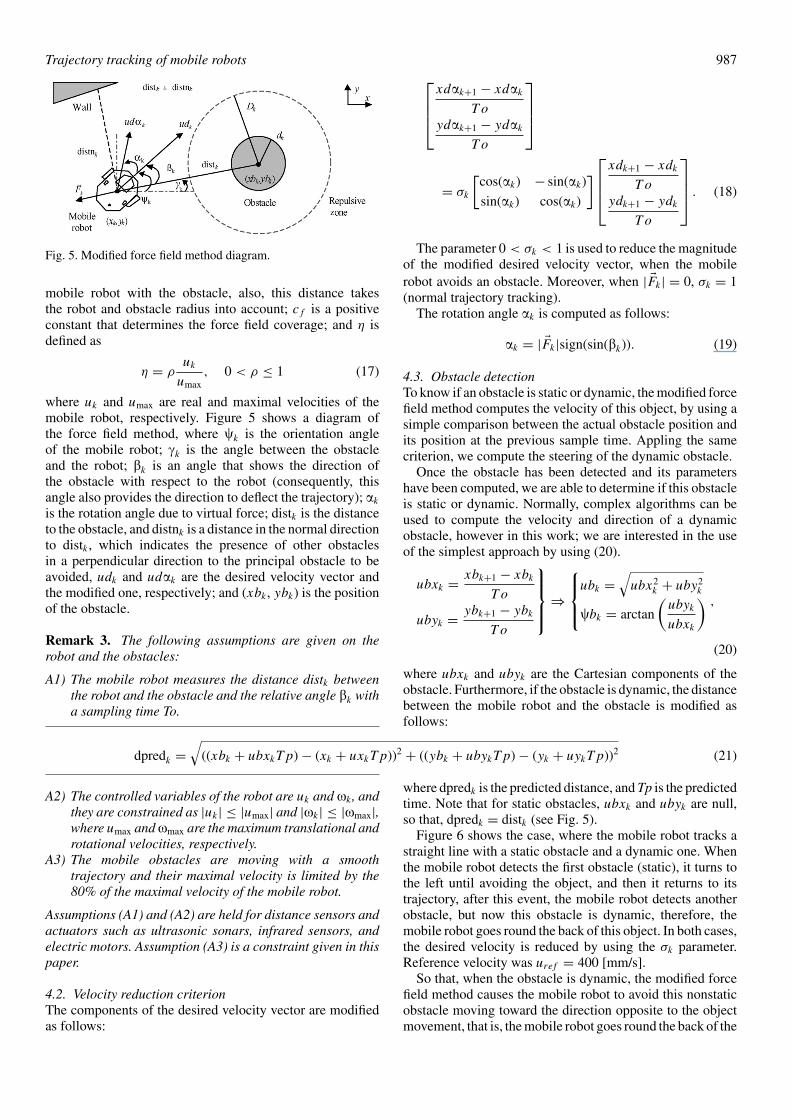
Fig. 5. Modified force field method diagram.

mobile robot with the obstacle, also, this distance takesthe robot and obstacle radius into account; cf is a positiveconstant that determines the force field coverage; and η isdefined as

η = ρuk

umax, 0 < ρ ≤ 1 (17)

where uk and umax are real and maximal velocities of themobile robot, respectively. Figure 5 shows a diagram ofthe force field method, where ψk is the orientation angleof the mobile robot; γk is the angle between the obstacleand the robot; βk is an angle that shows the direction ofthe obstacle with respect to the robot (consequently, thisangle also provides the direction to deflect the trajectory); αk

is the rotation angle due to virtual force; distk is the distanceto the obstacle, and distnk is a distance in the normal directionto distk , which indicates the presence of other obstaclesin a perpendicular direction to the principal obstacle to beavoided, udk and udαk are the desired velocity vector andthe modified one, respectively; and (xbk , ybk) is the positionof the obstacle.

Remark 3. The following assumptions are given on therobot and the obstacles:

A1) The mobile robot measures the distance distk betweenthe robot and the obstacle and the relative angle βk witha sampling time To.

A2) The controlled variables of the robot are uk and ωk , andthey are constrained as |uk| ≤ |umax| and |ωk| ≤ |ωmax|,where umax andωmax are the maximum translational androtational velocities, respectively.

A3) The mobile obstacles are moving with a smoothtrajectory and their maximal velocity is limited by the80% of the maximal velocity of the mobile robot.

Assumptions (A1) and (A2) are held for distance sensors andactuators such as ultrasonic sonars, infrared sensors, andelectric motors. Assumption (A3) is a constraint given in thispaper.

4.2. Velocity reduction criterionThe components of the desired velocity vector are modifiedas follows:

⎡⎢⎢⎣

xdαk+1 − xdαk

T o

ydαk+1 − ydαk

T o

⎤⎥⎥⎦

= σk

[cos(αk) − sin(αk)

sin(αk) cos(αk)

]⎡⎢⎢⎣

xdk+1 − xdk

T o

ydk+1 − ydk

T o

⎤⎥⎥⎦ . (18)

The parameter 0 < σk < 1 is used to reduce the magnitudeof the modified desired velocity vector, when the mobilerobot avoids an obstacle. Moreover, when | �Fk| = 0, σk = 1(normal trajectory tracking).

The rotation angle αk is computed as follows:

αk = | �Fk|sign(sin(βk)). (19)

4.3. Obstacle detectionTo know if an obstacle is static or dynamic, the modified forcefield method computes the velocity of this object, by using asimple comparison between the actual obstacle position andits position at the previous sample time. Appling the samecriterion, we compute the steering of the dynamic obstacle.

Once the obstacle has been detected and its parametershave been computed, we are able to determine if this obstacleis static or dynamic. Normally, complex algorithms can beused to compute the velocity and direction of a dynamicobstacle, however in this work; we are interested in the useof the simplest approach by using (20).

ubxk = xbk+1 − xbk

T o

ubyk = ybk+1 − ybk

T o

⎫⎪⎪⎬⎪⎪⎭ ⇒

⎧⎪⎨⎪⎩

ubk =√

ubx2k + uby2

k

ψbk = arctan

(ubyk

ubxk

),

(20)

where ubxk and ubyk are the Cartesian components of theobstacle. Furthermore, if the obstacle is dynamic, the distancebetween the mobile robot and the obstacle is modified asfollows:

dpredk =√

((xbk + ubxkTp) − (xk + uxkTp))2 + ((ybk + ubykTp) − (yk + uykTp))2 (21)

where dpredk is the predicted distance, and Tp is the predictedtime. Note that for static obstacles, ubxk and ubyk are null,so that, dpredk = distk (see Fig. 5).

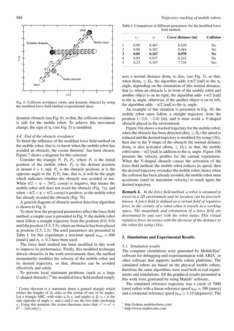
Figure 6 shows the case, where the mobile robot tracks astraight line with a static obstacle and a dynamic one. Whenthe mobile robot detects the first obstacle (static), it turns tothe left until avoiding the object, and then it returns to itstrajectory, after this event, the mobile robot detects anotherobstacle, but now this obstacle is dynamic, therefore, themobile robot goes round the back of this object. In both cases,the desired velocity is reduced by using the σk parameter.Reference velocity was uref = 400 [mm/s].

So that, when the obstacle is dynamic, the modified forcefield method causes the mobile robot to avoid this nonstaticobstacle moving toward the direction opposite to the objectmovement, that is, the mobile robot goes round the back of the

988 Trajectory tracking of mobile robots

Fig. 6. Collision avoidance (static and dynamic objects) by usingthe modified force field method (experimental data).

dynamic obstacle (see Fig. 6), so that, the collision avoidanceis safe for the mobile robot. To achieve this movementchange, the sign of αk (see Fig. 5) is modified.

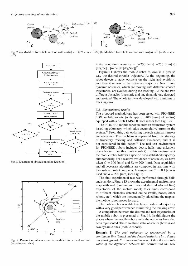
4.4. End of the obstacle avoidanceTo finish the influence of the modified force field method onthe mobile robot, that is, to know when the mobile robot hasavoided an obstacle, the cosine theorem* has been chosen.Figure 7 shows a diagram for this criterion.

Consider the triangle Pr Pd Po, where Pr is the initialposition of the mobile robot; Pd is the desired positionat instant k + 1; and, Po is the obstacle position; ϕ is theopposite angle to the PrPd line, that is, it will be the anglewhich indicates whether the obstacle was avoided or not.When π/2 < ϕ < 3π/2, cos(ϕ) is negative, that means themobile robot still does not avoid the obstacle (Fig. 7a), andwhen −π/2 < ϕ< π/2, cos(ϕ) is positive, so the mobile robothas already avoided the obstacle (Fig. 7b).

A general diagram of obstacle motion detection algorithmis shown in Fig. 8.

To show how the proposed parameters affect the force fieldmethod, a simple case is presented in Fig. 9: the mobile robotmust follow a straight trajectory from the position (0.0, 0.0)until the position (5.5, 5.5), where an obstacle has been placedat position (2.5, 2.5). The used parameters are presented inTable I, for this experiment a maximal speed umax = 600[mm/s] and σk = 0.2 have been used.

The force field method has been modified in this workto improve its performance. Firstly, this modified techniquedetects obstacles in the work environment; then, the methodmomentarily modifies the velocity of the mobile robot andits desired trajectory, so that, obstacles can be avoidedeffectively and safely.

To prevent local minimum problems (such as a largeU-shaped obstacle),29 the modified force field method simply

* Cosine theorem is a statement about a general triangle whichrelates the lengths of its sides to the cosine of one of its angles.Let a triangle ABC, with sides a, b, c, and angles α, β, γ; c is theside opposite of angle γ , and a and b are the two sides enclosingγ . Using this notation, the cosine theorems states that: c2 = a2 +b2 − 2ab cos(γ ).

Table I. Comparison of different parameters for the modified forcefield method..

cf ρ Cover distance [m] Collision

1 0.99 0.467 8.630 No2 0.99 0.167 8.484 No3 0.85 0.167 8.078 No4 0.85 0.937 8.243 No5 0.23 0.167 7.716 Yes

uses a normal distance distnk to distk (see Fig. 5), so that,when distnk ≤ Dk , the algorithm adds ±π/2 [rad] to the αk

angle, depending on the orientation of this normal distance,that is, when an obstacle is in front of the mobile robot andanother object is on its right, the algorithm adds +π/2 [rad]to the αk angle, otherwise, if the another object is on its left,the algorithm adds −π/2 [rad] to the αk angle.

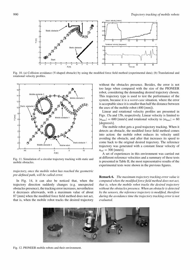
An example of this situation is presented in Fig. 10: themobile robot must follow a straight trajectory from theposition (−2.0, −2.0) [m], and it must avoid a V-shapedobstacle placed in the environment.

Figure 10a shows a tracked trajectory for the mobile robot;when the obstacle has been detected (distk ≤ Dk) the speed isreduced and the desired trajectory is modified (by using (18)),then due to the V-shape of the obstacle the normal distancedistnk is also activated (distnk ≤ Dk), so that, the mobilerobot turns −π/2 [rad] in addition to the αk angle. Figure 10bpresents the velocity profiles for the current experiment.When the V-shaped obstacle causes the activation of theforce field method, the mobile robot reduces its speed, thenthe desired trajectory overtakes the mobile robot, hence whenthe collision has been already avoided, the mobile robot mustaccelerate (until its maximum velocity) to reach again thedesired trajectory.

Remark 4. In the force field method, a robot is assumed totravel in a 2D environment and its location can be preciselyknown. A force field is defined as a virtual field of repulsiveforce in the vicinity of a robot when it travels in a workingspace. The magnitude and orientation of a force field aredetermined by and vary with the robot status. This virtualrepulsive force increases with the decrease of the distance tothe robot (by using (16)).

5. Simulations and Experimental Results

5.1. Simulation resultsThe computer simulations were generated by MobileSim*

software for debugging and experimentation with ARIA∗

orother software that supports mobile robots platforms. Thesimulated robots are based on the physical mobile robots;therefore the same algorithms were used both in real experi-ments and simulations. All the graphical results presented inthis work were generated by using Matlab† software.

The simulated reference trajectory was a circle of 7000[mm] radius with a linear reference speed uref = 390 [mm/s]and a rotational reference speed ωref = 3.19 [degrees/s]. The

* http://robots.mobilerobots.com/† http://www.mathworks.com

Trajectory tracking of mobile robots 989

Fig. 7. (a) Modified force field method with cos(ϕ) < 0 (π/2 < ϕ < 3π/2) (b) Modified force field method with cos(ϕ) > 0 (−π/2 < ϕ <π/2).

Fig. 8. Diagram of obstacle motion detection.

Fig. 9. Parameters influence on the modified force field method(experimental data).

initial conditions were x0 = [−250 [mm] −250 [mm] 0[degree] 0 [mm/s] 0 [deg/sec]]T .

Figure 11 shows the mobile robot follows in a preciseway the desired circular trajectory. At the beginning, therobot detects a static obstacle on the right and avoids it,and then it returns to the reference trajectory. Next, threedynamic obstacles, which are moving with different smoothtrajectories, are avoided during the tracking. At the end twodifferent obstacles (one static and one dynamic) are detectedand avoided. The whole test was developed with a minimumtracking error.

5.2. Experimental resultsThe proposed methodology has been tested with PIONEER3DX mobile robots (with approx. 400 [mm] of radius)equipped with a SICK LMS200 laser sensor (see Fig. 12).

The PIONEER mobile robot includes an estimation systembased on odometry, which adds accumulative errors to thesystem.33 From this, data updating through external sensorsare necessary. This problem is separated from the strategyof trajectory tracking and collision avoidance, and it isnot considered in this paper.31 The real test environmentfor PIONEER robots includes doors, halls, and unknownobstacles (e.g. another mobile robot). In this environmentthe mobile robot follows a specific pre-established trajectoryautonomously. For a reactive avoidance of obstacles, we havetaken dk = 300 [mm] and Dk = 700 [mm]. Data acquisitionand all necessary algorithms are computed in real time withthe on-board robot computer. A sample time To = 0.1 [s] wasused and a = 200 [mm] (see Fig. 1).

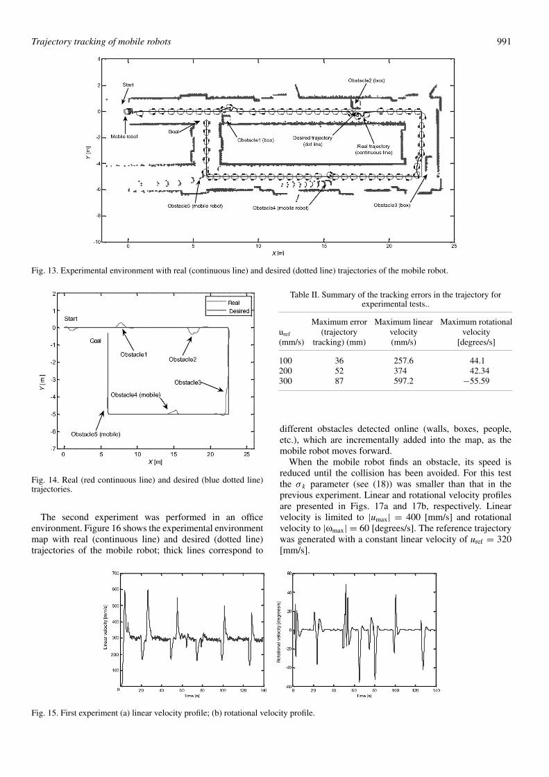
The first experimental test was performed through hallsand corridors. Figure 13 shows the experimental environmentmap with real (continuous line) and desired (dotted line)trajectories of the mobile robot; thick lines correspondto different obstacles detected online (walls, boxes, otherrobots, etc.), which are incrementally added into the map, asthe mobile robot moves forward.

The mobile robot was able to achieve the desired trajectorywith a very good performance minimizing the tracking error.

A comparison between the desired and real trajectories ofthe mobile robot is presented in Fig. 14. In this figure theplaces where the mobile robot avoids the obstacles have alsobeen represented. There are three static obstacles (boxes) andtwo dynamic ones (mobile robots).

Remark 5. The real trajectory is represented by acontinuous line (black) and the desired trajectory by a dottedone (dark green). It is important to remark that the absolutevalue of the difference between the desired and the real

990 Trajectory tracking of mobile robots

Fig. 10. (a) Collision avoidance (V-shaped obstacle) by using the modified force field method (experimental data); (b) Translational androtational velocity profiles.

Fig. 11. Simulation of a circular trajectory tracking with static andmobile obstacles.

trajectory, once the mobile robot has reached the geometricpre-defined path, will be called error.

In Fig. 14, it can also be noticed that, when thetrajectory direction suddenly changes (e.g. unexpectedobstacles presence), the tracking error increases, neverthelessit decreases afterwards, with a maximum value of about87 [mm] when the modified force field method does not act,that is, when the mobile robot tracks the desired trajectory

without the obstacles presence. Besides, the error is nottoo large when compared with the size of the PIONEERrobot, considering the demanding desired trajectory chosen.This trajectory type is used to test the performance of thesystem, because it is a worst-case situation, where the erroris acceptable since it is smaller than half the distance betweenthe axes of the mobile robot (400 [mm]).

Linear and rotational velocity profiles are presented inFigs. 15a and 15b, respectively. Linear velocity is limited to|umax| = 600 [mm/s] and rotational velocity to |ωmax| = 60[degrees/s].

The mobile robot gets a good trajectory tracking. When itdetects an obstacle, the modified force field method comesinto action: the mobile robot reduces its velocity untilavoiding the obstacle, and after that increases its speed tocome back to the original desired trajectory. The referencetrajectory was generated with a constant linear velocity ofuref = 300 [mm/s].

A set of experiences in this environment was carried outat different reference velocities and a summary of these testsis presented in Table II, the most representative results of theexperimental tests were shown in the previous figures.

Remark 6. The maximum trajectory tracking error value iscomputed when the modified force field method does not act,that is, when the mobile robot tracks the desired trajectorywithout the obstacles presence. When an obstacle is detectedby the sensors, the reference trajectory is modified, thereforeduring the avoidance time the trajectory tracking error is notevaluated.

Fig. 12. PIONEER mobile robots and their environment.

Trajectory tracking of mobile robots 991

Fig. 13. Experimental environment with real (continuous line) and desired (dotted line) trajectories of the mobile robot.

Fig. 14. Real (red continuous line) and desired (blue dotted line)trajectories.

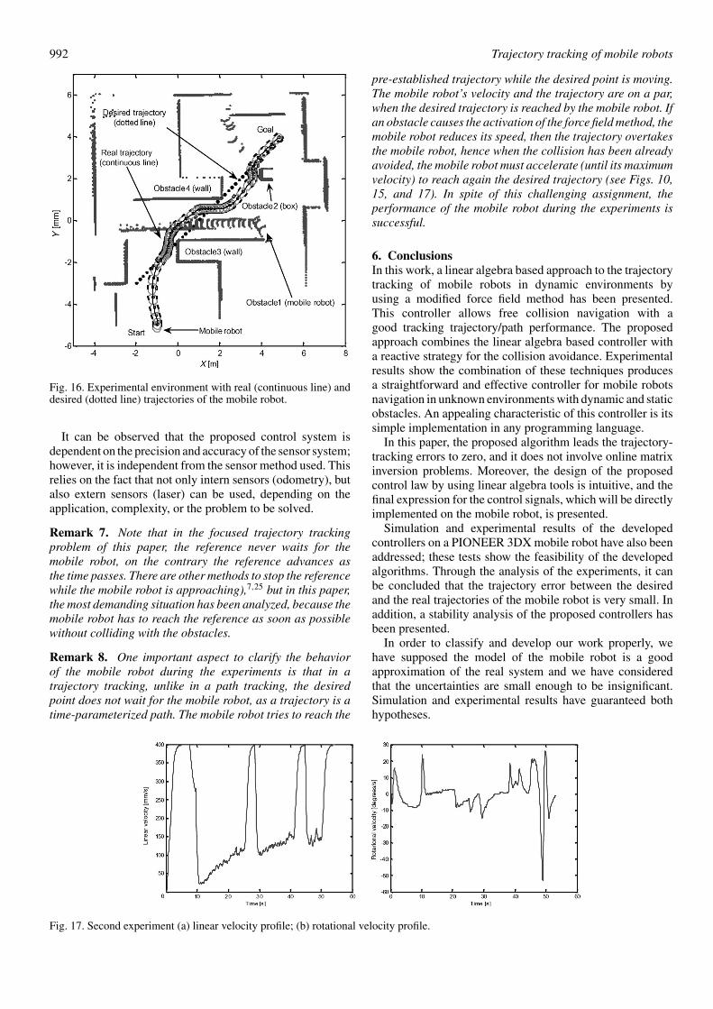
The second experiment was performed in an officeenvironment. Figure 16 shows the experimental environmentmap with real (continuous line) and desired (dotted line)trajectories of the mobile robot; thick lines correspond to

Table II. Summary of the tracking errors in the trajectory forexperimental tests..

Maximum error Maximum linear Maximum rotationaluref (trajectory velocity velocity(mm/s) tracking) (mm) (mm/s) [degrees/s]

100 36 257.6 44.1200 52 374 42.34300 87 597.2 −55.59

different obstacles detected online (walls, boxes, people,etc.), which are incrementally added into the map, as themobile robot moves forward.

When the mobile robot finds an obstacle, its speed isreduced until the collision has been avoided. For this testthe σ k parameter (see (18)) was smaller than that in theprevious experiment. Linear and rotational velocity profilesare presented in Figs. 17a and 17b, respectively. Linearvelocity is limited to |umax| = 400 [mm/s] and rotationalvelocity to |ωmax| = 60 [degrees/s]. The reference trajectorywas generated with a constant linear velocity of uref = 320[mm/s].

Fig. 15. First experiment (a) linear velocity profile; (b) rotational velocity profile.

992 Trajectory tracking of mobile robots

Fig. 16. Experimental environment with real (continuous line) anddesired (dotted line) trajectories of the mobile robot.

It can be observed that the proposed control system isdependent on the precision and accuracy of the sensor system;however, it is independent from the sensor method used. Thisrelies on the fact that not only intern sensors (odometry), butalso extern sensors (laser) can be used, depending on theapplication, complexity, or the problem to be solved.

Remark 7. Note that in the focused trajectory trackingproblem of this paper, the reference never waits for themobile robot, on the contrary the reference advances asthe time passes. There are other methods to stop the referencewhile the mobile robot is approaching),7,25 but in this paper,the most demanding situation has been analyzed, because themobile robot has to reach the reference as soon as possiblewithout colliding with the obstacles.

Remark 8. One important aspect to clarify the behaviorof the mobile robot during the experiments is that in atrajectory tracking, unlike in a path tracking, the desiredpoint does not wait for the mobile robot, as a trajectory is atime-parameterized path. The mobile robot tries to reach the

pre-established trajectory while the desired point is moving.The mobile robot’s velocity and the trajectory are on a par,when the desired trajectory is reached by the mobile robot. Ifan obstacle causes the activation of the force field method, themobile robot reduces its speed, then the trajectory overtakesthe mobile robot, hence when the collision has been alreadyavoided, the mobile robot must accelerate (until its maximumvelocity) to reach again the desired trajectory (see Figs. 10,15, and 17). In spite of this challenging assignment, theperformance of the mobile robot during the experiments issuccessful.

6. ConclusionsIn this work, a linear algebra based approach to the trajectorytracking of mobile robots in dynamic environments byusing a modified force field method has been presented.This controller allows free collision navigation with agood tracking trajectory/path performance. The proposedapproach combines the linear algebra based controller witha reactive strategy for the collision avoidance. Experimentalresults show the combination of these techniques producesa straightforward and effective controller for mobile robotsnavigation in unknown environments with dynamic and staticobstacles. An appealing characteristic of this controller is itssimple implementation in any programming language.

In this paper, the proposed algorithm leads the trajectory-tracking errors to zero, and it does not involve online matrixinversion problems. Moreover, the design of the proposedcontrol law by using linear algebra tools is intuitive, and thefinal expression for the control signals, which will be directlyimplemented on the mobile robot, is presented.

Simulation and experimental results of the developedcontrollers on a PIONEER 3DX mobile robot have also beenaddressed; these tests show the feasibility of the developedalgorithms. Through the analysis of the experiments, it canbe concluded that the trajectory error between the desiredand the real trajectories of the mobile robot is very small. Inaddition, a stability analysis of the proposed controllers hasbeen presented.

In order to classify and develop our work properly, wehave supposed the model of the mobile robot is a goodapproximation of the real system and we have consideredthat the uncertainties are small enough to be insignificant.Simulation and experimental results have guaranteed bothhypotheses.

Fig. 17. Second experiment (a) linear velocity profile; (b) rotational velocity profile.

Trajectory tracking of mobile robots 993

The proposed methodology for the controller design can beapplied to other types of systems. The required precision ofthe proposed numerical method for the system approximationis smaller than the one needed to simulate the behavior ofthe system. This is because, when the states for the feedbackare available, in each sampling time, any difference fromaccumulative errors is corrected (e.g. rounding errors). Thus,the approach is used to find the best way to go from one stateto the next one, according to the availability of the systemmodel.

Appendix: Stability AnalysisThis appendix provides the stability analysis of theproposed controller. The used criterions to demonstrate theconvergence of the proposed algorithms are mainly based onref. [1].

Condition for zero-error convergence: In order to analyzethe stability of the proposed controller, the system (11)–(14)will be used again. By analyzing this system the requiredconditions for a zero-error convergence will be provided.⎡

⎢⎣cos(ψk) −a sin(ψk)

sin(ψk) a cos(ψk)

0 1

⎤⎥⎦

︸ ︷︷ ︸B

[uk

ωk

]︸ ︷︷ ︸

υ

= 1

T o

⎡⎢⎣�x

�y

�ψ

⎤⎥⎦

︸ ︷︷ ︸c

, (A1)

where �x = xdk+1 − xk , �y = ydk+1 − yk , and �ψ =ψdk+1 − ψk .

The desired orientation for the mobile robot mustguarantee that nonholonomic system reaches the pre-established trajectory with a zero-error convergence. Tocompute this required orientation, the column space criterionwill be again used. Subsequently, system (A1) must have anexact solution. To fulfil this condition, vector c is obliged tobelong to column space of matrix B, that is, vector c has tobe a linear combination of column vectors of matrix B.43

A column space base of the matrix B, C(B) is given by

C(B) =

⎧⎪⎨⎪⎩

⎡⎢⎣cos(ψk)

sin(ψk)

0

⎤⎥⎦ ,

⎡⎢⎣−a sin(ψk)

a cos(ψk)

1

⎤⎥⎦

⎫⎪⎬⎪⎭ . (A2)

The orthonormal column space base of the matrix B, C⊥(B)is given by

C⊥(B) =

⎧⎪⎨⎪⎩

⎡⎢⎣cos(ψk)

sin(ψk)

0

⎤⎥⎦ ,

1√a2 + 1

⎡⎢⎣−a sin(ψk)

a cos(ψk)

1

⎤⎥⎦

⎫⎪⎬⎪⎭

= {w1, w2}. (A3)

Vector c of (A1) is composed of two parts: the componentin the column space cC(B) and the component in the left nullspace cN(BT ) of the matrix B, that is

c = cC(B) + cN(BT ) (A4)

cC(B) = (cT w1)w1 + (cT w2)w2 (A5)

cC(B) = 1

T o

⎡⎣�x cos2(ψk) + �y sin(ψk) cos(ψk)

�x sin(ψk) cos(ψk) + �y sin2(ψk)0

⎤⎦ + 1

T o(at2 + 1)

×

⎡⎢⎣

a2�x sin2(ψk) − a2�y sin(ψ(k)) cos(ψk) − a�ψ sin(ψk)

−a2�x sin(ψk) cos(ψk) + a2�y cos2(ψk) + a�ψ cos(ψk)

−a�x sin(ψk) + a�y cos(ψk) + �ψ

⎤⎥⎦ .

(A6)

For an exact solution, c must be equal to cC (B), that is

cC(B) = 1

T o[�x �y �ψ]T . (A7)

Operating and simplifying some terms in the aboveequation, the following condition is obtained:

⎡⎣ sin(ψk)(�x sin(ψk) − �y cos(ψk) + a�ψ)

cos(ψk)(−�x sin(ψk) + �y cos(ψk) − a�ψ)a�ψ+ �x sin(ψk) − �y cos(ψk)

⎤⎦ =

⎡⎣0

00

⎤⎦ .

(A8)

That is,

�x sin(ψk) − �y cos(ψk) + a�ψ = 0. (A9)

From (A9), the required angle to the error converges tozero can be obtained,

ψezk+1 = ψk − �x sin(ψk) − �y cos(ψk)

a, (A10)

where ψezk is the angle for a zero-error convergence.From (A10), the following relation is obtained; this

expression will be used for future computations:

a(ψezk+1 − ψk) = −�x sin(ψk) + �y cos(ψk). (A11)

Assumption 1. Because the reference velocities uref and ωref

satisfy (2), the mobile robot can follow a pre-establishedtrajectory. Moreover, the reference trajectory also fulfils(A1), that is

xrefk+1 = xrefk + urefkT o cos(ψrefk) − ωrefkaT o sin(ψrefk)

yrefk+1 = yrefk + urefkT o sin(ψrefk) + ωrefkaT o cos(ψrefk)

ψrefk+1 = ψrefk + T oωrefk (A12)

where variables xref , yref , ψref , uref , and ωref are thereference state variables that composed the pre-establishedtrajectory.

Assumption 2. So that the error tends to zero, the followingrelations for the desired variables are proposed:

xdk+1 = xref k+1 − kx (xref k − xk)︸ ︷︷ ︸xk

ydk+1

= yref k+1 − ky (yref k − yk)︸ ︷︷ ︸yk

ψdk+1

= ψrefk+1 − kψ (ψref k − ψk)︸ ︷︷ ︸ψk

(A13)

994 Trajectory tracking of mobile robots

where x, y, and ψ are the errors in x, y, and ψ, respectively;kx , ky , and kψ are constants of weight for x, y, and ψ,respectively. Also, 0 < (kx, ky, kψ) < 1.

Additionally, to achieve the zero-error convergencecondition the reference orientation angle ψrefk in (A13) willbe replaced with the zero-error convergence angle ψek , thatis,

ψdk+1 = ψek+1 − kψ (ψek − ψk)︸ ︷︷ ︸ψk

. (A14)

Assumption 3. Translational and rotational real velocitieswill be equal to the linear and rotational desired velocities,respectively, plus the particular error for each case, that is,

uk = udk + uk (A15)ωk = ωdk + ωk

where u and ω are the errors in u and ω, respectively.Analysis for ψ: From (A14), and by using �ψ = ψdk+1

−ψk

�ψ = (ψek+1 − ψk) − kψψk (A16)

From (10), (15), and (A15),

ψk+1 = ψk + T oωk = ψk

+−a�x sin(ψk) + a�y cos(ψk) + �ψ

a2 + 1+ T oωk (A17)

From (A16) and (A17), and by using (A11),

ψk+1 = ψk

+ a2(ψek+1 − ψk) + (ψek+1 − ψk) − kψψk

a2 + 1+ T oωk

ψk+1 = ψek+1 − 1

a2 + 1kψψk + T oωk

(ψek+1 − ψk+1)︸ ︷︷ ︸ψk+1

− 1

a2 + 1kψψk + T oωk = 0

ψk+1 − 1

a2 + 1kψψk + T oωk = 0 (A18)

By the analysis of (A18), it can be concluded that if ωk → 0with k → ∞, then ψk → 0 with k → ∞. Therefore, todemonstrate the stability of ψ, the stability of ω also must beverified.

Before verifying the stability of ω, an analysis for x and ywill be carried out.Analysis for x and y: First the state x will be analyzed.

From (10), (15), and (A15),

xk+1 = xk + [�x cos2(ψk) + �y sin(ψk) cos(ψk)]

+ T o cos(ψk)uk − sin(ψk)

a2 + 1

× [−a2�x sin(ψk) + a2�y cos(ψk) + a�ψ]

− aT o sin(ψk)ωk (A19)

Replacing (A11) in (A19)

xk+1 = xk + [�x cos2(ψk) + �y sin(ψk) cos(ψk)]

+ T o cos(ψk)uk − aT o sin(ψk)ωk

− sin(ψk)

a2 + 1[−a2�x sin(ψk) + a2�y cos(ψk)

+ a(ψezk+1 − ψk) − akψψk]

Again, by using (A11) in the above equation

xk+1 = xk + �x + a

a2 + 1sin(ψk)kψψk

+T o cos(ψk)uk − aT o sin(ψk)ωk

Replacing the expression xdk+1 = xk + �x in the previousequation

xk+1 = xdk+1 + a

a2 + 1sin(ψk)kψψk + T o cos(ψk)uk

−aT o sin(ψk)ωk. (A20)

Finally, replacing (A13) in (A20) the expression for thex-error is obtained,

xk+1 = xref k+1 − kxxk + a

a2 + 1sin(ψk)kψψk

+ T o cos(ψk)uk − aT o sin(ψk)ωk

(xref k+1 − xk+1) − kxxk + a

a2 + 1sin(ψk)kψψk

+ T o cos(ψk)uk − aT o sin(ψk)ωk = 0

So,

xk+1 − kxxk

+ a

a2 + 1sin(ψk)kψψk + T o cos(ψk)uk−aT o sin(ψk)ωk︸ ︷︷ ︸

nonlinearity

= 0

(A21)If a similar analysis is carried out for the state y, an analogousexpression to (A21) will be obtain, that is

yk+1 − kyyk

− a

a2 + 1cos(ψk)kψψk+T o sin(ψk)uk+aT o cos(ψk)ωk︸ ︷︷ ︸

nonlinearity

= 0.

(A22)So that, from (A21) and (A22),[

xk+1

yk+1

]=

[kx 00 ky

] [xk

yk

]

+ a

a2 + 1

[− sin(ψk)

cos(ψk)

]kψψk + T o

[cos(ψk) −a sin(ψk)

sin(ψk) a cos(ψk)

] [uk

ωk

]︸ ︷︷ ︸

nonlinearity

.

(A23)

Trajectory tracking of mobile robots 995

By analyzing (A23), it can be concluded that if the non-linearity behavior is bounded and uk → 0 and ωk → 0 withk → ∞, then xk → 0 and yk → 0 with k → ∞. Therefore,like in the case of ψ, the stability of x and y also depends onthe stability of u and ω.

Analysis for u andω: From (2), the states u andω at instantk+1, will be given by

[uk+1

ωk+1

]=

[uk

ωk

]+ T o

⎡⎢⎢⎣

θ3

θ1ω2

k − θ4

θ1uk

−θ5

θ2ukωk − θ6

θ2ωk

⎤⎥⎥⎦

+T o

⎡⎢⎣

1

θ10

01

θ2

⎤⎥⎦

[uck

ωck

](A24)

Replacing the controller expression (7) in (A24)

[uk+1

ωk+1

]=

[uk

ωk

]+ T o

⎡⎢⎢⎣

θ3

θ1ω2

k − θ4

θ1uk

−θ5

θ2ukωk − θ6

θ2ωk

⎤⎥⎥⎦ +

⎡⎢⎣

1

θ10

01

θ2

⎤⎥⎦

×[θ1udk+1 − (θ1 − T oθ4)uk − T oθ3ω

2k

θ2ωdk+1 − (θ2 − T0θ6)ωk + T0θ5ukωk

]

[uk+1

ωk+1

]=

[uk

ωk

]+ T o

⎡⎢⎢⎣

θ3

θ1ω2

k − θ4

θ1uk

−θ5

θ2ukωk − θ6

θ2ωk

⎤⎥⎥⎦

+

⎡⎢⎢⎣

udk+1 −(

1 − T oθ4

θ1

)uk − T o

θ3

θ1ω2

k

ωdk+1 −(

1 − T oθ6

θ2

)ωk + T o

θ5

θ2ukωk

⎤⎥⎥⎦

So, [uk+1

ωk+1

]=

[udk+1

ωdk+1

](A25)

Assumption 4. So that the error tends to zero, the followingrelations for the desired variables are proposed:

udk+1 = uref k+1 − ku (uref k − uk)︸ ︷︷ ︸uk

ωdk+1 = ωref k+1 − kω (ωref k − ωk)︸ ︷︷ ︸ωk

, (A26)

where ku and kω are constants of weight for u and ω,respectively. Also, 0 < (ku, kω) < 1. Replacing (A26) in(A25)

[uk+1

ωk+1

]=

[uref k+1 − kuuk

ωref k+1 − kωωk

].

So, [uk+1 − kuuk

ωk+1 − kωωk

]=

[0

0

]. (A27)

Therefore, from (A27), it is concluded uk → 0 ands ωk → 0with k → ∞. Now, the behavior of the nonlinearity in (A23)for x and y will be analyzed.

Analysis of the nonlinearity in x and y: Equation (A23) canbe written as

vk+1 = Avk + Pk (A28)

where

vk =[xk

yk

], A =

[kx 0

0 ky

]

Pk = a

a2 + 1

[− sin(ψk)cos(ψk)

]kψψk =

[P 1k

P 2k

]ψk and

Qk = T o

[cos(ψk) −a sin(ψk)sin(ψk) a cos(ψk)

] [uk

ωk

]

Matrices P(k) and Q(k) are limited and from (A18) and (A27),

limk→∞

ψk = 0, limk→∞

uk = 0, and limk→∞

ωk = 0 (A29)

So that, it is true that Pk → 0 and Qk → 0 with k → ∞.

Proof. By using ref. [1, Theorem 5.3.1, p. 248 andTheorem 5.2.3, p. 240], each solution vk of (A28) satisfies

vk = Akv0 +k∑

l=1

Ak−l [Pl−1 + Ql−1] (A30)

vk = Akv0 +k∑

l=1

Ak−lPl−1+k∑

l=1

Ak−lQl−1 (A31)

‖vk‖ ≤ ∥∥Akv0

∥∥ +∥∥∥∥∥

k∑l=1

Ak−lPl−1

∥∥∥∥∥ +∥∥∥∥∥

k∑l=1

Ak−lQl−1

∥∥∥∥∥(A32)

Equation (A31) can be written as

‖vk‖ ≤ c0 [δ (1 + c2)]k−k1

+∥∥∥∥∥

k∑l=1

Ak−lPl−1

∥∥∥∥∥ +∥∥∥∥∥

k∑l=1

Ak−lQl−1

∥∥∥∥∥ (A33)

where∥∥∥∥∥k∑

l=1

Ak−lPl−1

∥∥∥∥∥≤ max√(

P 12k + P 22

k

) ∣∣ψ0

∣∣ ∥∥∥∥∥k∑

l=1

Ak−lkl−1ψ

∥∥∥∥∥(A34)

∥∥∥∥∥k∑

l=1

Ak−lQl−1

∥∥∥∥∥ ≤ |u0|∥∥∥∥∥

k∑l=1

Ak−lkl−1u

∥∥∥∥∥+|ω0|∥∥∥∥∥

k∑l=1

Ak−lkl−1ω

∥∥∥∥∥(A35)

996 Trajectory tracking of mobile robots

where ψ0, u0 and ω0 are the initial angle and velocities errors,respectively, and 0 < (kψ, ku, kω) < 1. We can always chooseδ(1 + c2) < 1 according to ref. [1, Theorem 5.2.3, pp. 240–241], and applying the Toeplitz Lemma ref. [1, p. 682], it istrue that,

limk→∞

k∑l=1

Ak−lkl−1ψ = 0, lim

k→∞

k∑l=1

Ak−lkl−1u = 0,

limk→∞

k∑l=1

Ak−lkl−1ω = 0 (A36)

Then, from (A32–A36),

limk→∞

‖vk‖ = 0 (A37)

Subsequently, from (A23), (A28), and (A37) xk → 0, yk →0, and ψk → 0 with k → ∞.

Remark A1. If the trajectory tracking problem with uref =0 is considered:

‖xk‖ = ‖[xk yk ψk uk ωk]T ‖ → 0 with k → ∞.

Remark A2. If the positioning problem with uref = 0is considered, by using ref. [1, Theorem 5.3.1, Chapter 5,p. 248] it is also fulfilled that

‖xk‖ = ‖[xk yk ψk uk ωk]T ‖ → 0 with k → ∞.

Remark A3. The necessary and sufficient condition for thesystem (A1) has a zero-error convergence is (A9), becausethis condition causes an exact solution in the aforementionedsystem.

AcknowledgmentsThis work was partially funded by the German AcademicExchange Service (DAAD – Deutscher Akademischer Aus-tausch Dients), by the Consejo Nacional de InvestigacionesCientıficas y Tecnicas (CONICET – National Council forScientific Research), and by the Universidad Nacional deSan Juan – UNSJ, Argentina. We would also like toacknowledge cooperation from the RTS – Institute forSystems Engineering, University of Hannover, Germany,especially to Prof. Dr.-Eng. Bernardo Wagner.

References1. R. Agarwal, Difference Equations and Inequalities, Theory,

Methods, and Applications (Marcel Dekker, Inc., New York,2000).

2. J. Borenstein and Y. Koren, “The vector field histogram-fast obstacle avoidance for mobile robots,” IEEE Trans. Rob.Automat. 7, 278–288 (1991).

3. R. Carelli, J. Santos-Victor, F. Roberti and S. Tosetti, “Directvisual tracking control of remote cellular robots,” Rob.Autonom. Syst. 54, 805–814 (2006).

4. J. H. Chung, B. J. Yi, W. K. Kim and H. Lee, “The DynamicModeling and Analysis for an Omnidirectional Mobile Robot

with Three Caster Wheels,” Proceedings of IEEE InternationalConference on Robotics and Automation, Taipei, Taiwan(2003) pp. 521–527.

5. C. Connolly, J. Burns and R. Weiss, “Path planning usingLaplace’s equation,” Proceedings of IEEE InternationalConference on Robotics and Automation, Cincinnati, Ohio(1990) pp. 2102–2106.

6. C. De la Cruz and R. Carelli, “Dynamic model based formationcontrol and obstacle avoidance of multi-robot systems,”Robotica 26, 345–356 (2008) (Cambridge).

7. F. Del Rio, G. Jimenez, J. Sevillano, C. Amaya and A. Balcells,“Error Adaptive Tracking for Mobile Robots,” Proceedingsof 28th Annual Conference on IEEE Industrial ElectronicsSociety, Sevilla, Spain (2002) pp. 1–42415–2420.

8. K. Do and J. Pan, “Global output-feedback path tracking ofunicycle-type mobile robots,” Rob. Comput.-Integr. Manuf. 22,166–179 (2006).

9. W. Dong and Y. Guo, “Dynamic Tracking Control of UncertainMobile Robots,” IEEE/RSJ International Conference onIntelligent Robots and Systems, Alberta, Canada (2005) pp.2774–2779.

10. R. Fierro and F. L. Lewis, “Control of a nonholonomic mobilerobot using neural networks,” IEEE Trans. Neural Network 9,589–600 (1998).

11. R. Fierro and F. L. Lewis, “Control of a nonholonomic mobilerobot: Backstepping kinematics into dynamics,” J. Rob. Syst.4, 149–163 (1997).

12. D. Fox, W. Burgard and S. Thrun, “The dynamic windowapproach to collision avoidance,” IEEE Rob. Automat. Mag. 4,23–33 (1997).

13. T. Fraichard and H. Asama, “Inevitable Collision States: AStep Towards Safer Robots?,” IEEE International Conferenceon Intelligent Robots and Systems, Las Vegas, Nevada, IROS(2003).

14. T. Fraichard and A. Scheuer, “Car-Like Robots and MovingObstacles,” IEEE International Conference on Robotics andAutomation, San Diego, California, ICRA (1994).

15. T. Fukao, H. Nakagawa and N. Adachi, “Adaptive trackingcontrol of a nonholonomic mobile robot,” IEEE Trans. Rob.Automat. 16, 609–615 (2000).

16. S. Ge and Y. Cui, “Dynamic motion planning for mobile robotsusing potential field method,” Autonom. Rob. 13, 207–222(2002).

17. C. L. Hwang and L. J. Chang, “Trajectory tracking and obstacleavoidance of car-like mobile robots in an intelligent space usingmixed H2/H∞ decentralized control,” Trans. Mechatron. 12,345–352 (2007).

18. C. L. Hwang, S. Y. Han and L. J. Chang, “Trajectory Trackingof Car-Like Mobile Robots using Mixed H2/H∞ DecentralizedVariable Structure Control,” International Conference onMechatronics, Chongqing, China (2005) pp. 520–525.

19. E. Jang, S. Jung and T. Hsia, “Collision Avoidance andControl of a Mobile Robot Using a Hybrid Force ControlAlgorithm”, 30th Annual Conference on IEEE IndustrialElectronics Society, Busan, Korea (2004) pp. 413–418.

20. S. Jung, E. Jang and T. Hsia, “Collision Avoidance of a MobileRobot Using Intelligent Hybrid Force Control Technique,”Proceedings of IEEE International Conference on Roboticsand Automation, Barcelona, Spain (2005) pp. 4418–4423.

21. Y. Kanayama, Y. Kimura, F. Miyazaki and T. Noguchi, “AStable Tracking Control Method for an Autonomous MobileRobot,” Proceedings of IEEE International Conference onRobotics and Automation, Tsukuba, Japan (1990) pp. 384–389.

22. K. Kim, “Receding horizon tracking control for constrainedlinear continuous time-varying systems,” IEEE Proc. ControlTheory Appl. 150, 534–538 (2003).

23. G. Klancar and I. Skrjank, “Tracking-error model-basedpredictive control for mobile robots in real time,” Rob.Autonom. Syst. 55, 460–469 (2007).

24. J. C. Latombe, Robot Motion Planning, vol. 0124 (Kluwer,Dordrecht, The Netherlands, 1991).

Trajectory tracking of mobile robots 997

25. S. Lee and J. H. Park, “Virtual Trajectory in Tracking Controlof Mobile Robots,” Proceedings of IEEE/ASME InternationalConference on Advanced Intelligent Mechatronic, Kobe, Japan,AIM (2003).

26. S. Liu, H. Zhang, S. X. Yang and J. Yu, “Dynamic Control of aMobile Robot Using an Adaptive Neurodynamics and SlidingMode Strategy,” Proceedings of 5th Congress IntelligentControl and Automation, Hangzhou, China (2004) pp. 5007–5011.

27. Z. Y. Liu, R. H. Jing, X. Q. Ding and J. H. Li, “TrajectoryTracking Control of Wheeled Mobile Robots Based on theArtificial Potential Field,” Fourth International Conference onNatural Computation, Jinan, China (2008) pp. 382–387.

28. A. Masoud, “Using hybrid vector-harmonic potential fieldsfor multi-robot, multi-target navigation in a stationaryenvironment,” Proc. IEEE Int. Conf. Rob. Automat. 4, 3564–3571 (1996).

29. T. Myers and L. Vlacic, “Autonomous driving in a time-varyingenvironment,” IEEE Adv. Rob. Soc. Impacts 1, 53–58 (2005).

30. Y. K. Nak and R. Simmons, “The Lane-Curvature Method forLocal Obstacle Avoidance,” IEEE International Conference onRobotics and Automation, Geiranger, Norway, ICRA (1998).

31. J. Normey-Rico, I. Alcala, J. Gomez-Ortega and E. Camacho,“Mobile robot path tracking using PID controller,” ControlEng. Pract. 9, 1209–1214 (2001).

32. J. Normey-Rico, J. Gomez-Ortega and E. Camacho, “A Smith-predictor-based generalized predictive controller for mobilerobot path-tracking,” Control Eng. Pract. 7, 729–740 (1999).

33. L. Ojeda and J. Borenstein, “Reduction of Odometry Errorsin Over-constrained Mobile Robots,” Proceedings of the UGVTechnology Conference at the SPIE AeroSense Symposium,Orlando, Florida (2003) pp. 21–25.

34. E. Owen and L. Montano, “A Robocentric Motion Plannerfor Dynamic Environments Using the Velocity Space,” IEEEInternational Conference on Intelligent Robots and Systems,Beijing, China, IROS (2006).

35. A. Rosales, G. Scaglia, V. Mut and F. di Sciascio, “ControllerDesigned by Means of Numeric Methods for a BenchmarkProblem: RTAC (Rotational Translational Actuator),” IEEE –Electronics, Robotics and Automotive Mechanics Conference,Cuernavaca, Mexico (2006) pp. 97–104.

36. G. Scaglia, V. Mut, A. Rosales and O. Quintero, “TrackingControl of a Mobile Robot using Linear Interpolation,”International Conference on Integrated Modeling and Analysisin Applied Control and Automation – IMAACA, Buenos Aires,Argentina (2007).

37. G. Scaglia, O. Quintero, V. Mut and F. di Sciascio, NumericalMethods Based Controller Design for Mobile Robots (IFACWorld Congress, 2008).

38. G. Scaglia, O. Quintero, V. Mut and F. di Sciascio, NumericalMethods Based Controller design for Mobile Robots (Robotica– Cambridge University Press, Cambridge, UK, 2008).

39. M. Seder, K. Macek and I. Petrovic, “An Integrated Approachto Real Time Mobile Robot Control in Partially Known IndoorEnvironments,” Proceedings of 31st Annual Conference of the

IEEE Industrial Electronics Society, Raleigh, North Carolina(2005).

40. S. Shuli, “Designing approach on trajectory-tracking controlof mobile robot,” Rob. Comput.-Integr. Manuf. 21, 81–85(2005).

41. R. Simmons, “The Curvature–Velocity Method for LocalObstacle Avoidance,” IEEE International Conference onRobotics and Automation, Geiranger, Norway, ICRA (1996).

42. C. Stachniss and W. Burgard, “An integrated approach togoal directed obstacle avoidance under dynamic constraintsfor dynamic environments,” IEEE International Conferenceon Intelligent Robots and Systems, EPFL, Switzerland, IROS(2002).

43. G. Strang, Linear Algebra and Its Applications, 3rd ed. (MITAcademic Press, New York, 1980).

44. J. Tian, M. Gao and E. Lu, “Dynamic Collision AvoidancePath Planning for Mobile Robot Based on Multi-sensor DataFusion by Support Vector Machine,” International Conferenceon Mechatronics and Automation, Harbin, China, ICMA07(2007) pp. 2779–2783.

45. P. S. Tsai, L. S. Wang, F. R. Chang and T. F. Wu, “SystematicBackstepping Design for B-spline Trajectory Tracking Controlof the Mobile Robot in Hierarchical Model,” InternationalConference on Networking, Sensing and Control, Taipei,Taiwan (2004) pp. 713–718.

46. I. Ulrich and J. Borenstein, “VFH∗: Local obstacle avoidancewith look ahead verification,” Proc. IEEE Int. Conf. Rob.Automat. 3, 2505–2511 (2000).

47. I. Ulrich and J. Borenstein, “VFH+: Reliable obstacleavoidance for fast mobile robots,” Proc. IEEE Int. Conf. Rob.Automat. 2, 1572–1577 (1998).

48. S. Vougioukas, “Reactive Trajectory Tracking for MobileRobots based on Non Linear Model Predictive Control,”International Conference on Robotics and Automation, Torun,Poland (2007) pp. 3074–3079.

49. D. Wang, D. Liu and G. Dissanayake, “A Variable Speed ForceField Method for Multi-Robot Collaboration,” Proceedings ofInternational Conference on Intelligent Robots and Systems,China (2006) pp.2697–2702.

50. T. Y. Wang and C. C. Tsai, “Adaptive TrajectoryTracking Control of a Wheeled Mobile Robot viaLyapunov Techniques,” Annual Conference of IEEE IndustrialElectronics Society, Busan, Korea (2004) pp. 389–394.

51. J. M. Yang and J. H. Kim, “Sliding mode control for trajectoryof nonholonomic wheeled mobile robots,”, IEEE Trans. Rob.Automat. 15, 578–587 (1999).

52. X. Yang, K. He, M. Guo and B. Zhang, “An IntelligentPredictive Control Approach to Path Tracking Problem ofAutonomous Mobile Robot,” IEEE International Conferenceon Robotics and Automation, Beijing, China (1998) pp. 3301–3306.

53. Huai-Xiang Zhang, Guo-Jun Dai and Hong Zeng, “ATrajectory Tracking Control Method for NonholonomicMobile Robots,” International Conference on Wavelet Analysisand Pattern Recognition, Beijing, China (2007) pp. 7–11.