Trajectory Control of a Single Link Rigid-Flexible Manipulator Pedro Miguel Santos Pires Dissertação para obtenção do Grau de Mestre em Engenharia Mecânica Júri Presidente: Professor José Manuel Gutierrez Sá da Costa Orientador: Professor José Manuel Gutierrez Sá da Costa Co-Orientador: Professor Jorge Manuel Mateus Martins Vogal: Professor Miguel Afonso Dias de Ayala Botto Setembro - 2007

Welcome message from author
This document is posted to help you gain knowledge. Please leave a comment to let me know what you think about it! Share it to your friends and learn new things together.
Transcript
Trajectory Control of a Single Link Rigid-FlexibleManipulator
Pedro Miguel Santos Pires
Dissertação para obtenção do Grau de Mestre em
Engenharia Mecânica
Júri
Presidente: Professor José Manuel Gutierrez Sá da Costa
Orientador: Professor José Manuel Gutierrez Sá da Costa
Co-Orientador: Professor Jorge Manuel Mateus Martins
Vogal: Professor Miguel Afonso Dias de Ayala Botto
Setembro - 2007


Este trabalho reflecte as ideias dos seus
autores que, eventualmente, poderão não
coincidir com as do Instituto Superior Técnico.

Abstract
The primary goal of this work is to control the end-point position of a planar single link flexible robot
manipulator from point A to point B.
We first introduce the non-minimum phase problem of flexible manipulators. The simulation tools used,
which were developed by J. Martins are then presented. An experimental manipulator was also used to
test the control methods.
In this report, three control techniques were used. The first technique, introduced by M. Benosman
and G. Le Vey, searches for proper output trajectories with polynomial form. Those output trajectories are
obtained in order that the effects of the unstable zeros are completely cancelled.
The second technique was recently studied by A. P. Aguiar, J. P. Hespanha, and P. Kokotović called
path-following. The path-following with internal model control main objective is to steer a physical object
to converge to a geometric path. The secondary objective is to ensure that an object’s motion along the
path satisfies a given dynamic specification. Path-following technique ensures that the system is no longer
time dependent, this is suppressed by parameterizing the path with an auxiliary variable.
The last studied technique is the evolution of the methodology previously presented. The normal form
path following is a control methodology that can satisfy three tasks.
• Geometric task.
• Dynamic task.
• Boundedness of the zero dynamics states.
i
In the final section of this report we present the experimental results. There is also specified some
conclusions and analysis of the developed work, with a future work recommendation.
Keywords: Flexible robot manipulators, motion planing, path-following, internal model control, normal
form representation, vibration control.
ii
Resumo
O principal objectivo desta tese é controlar a posição do elemento terminal de um robô manipulador planar
flexível do ponto A para o ponto B.
Começamos por introduzir o problema de fase não mínima dos manipuladores flexíveis. As ferramentas
de simulação utilizadas, desenvolvidas por J. Martins são apresentadas. Apresentamos o manipulador
experimental usado para testar os vários métodos de controlo.
Nesta tese, utilizou-se três técnicas de controlo. A primeira técnica, introduzida por M. Benosman e
G. Le Vey, procura uma saída polinomial apropriada. Essa trajectória de saida é obtida de modo que os
efeitos dos zeros instáveis do sistema sejam cancelados.
A segunda técnica foi recentemente estudada por A. P. Aguiar, J. P. Hespanha, e P. Kokotović chamada
path-following. O objectivo principal do path-following com controlo por modelo interno, é levar um
objecto físico a convergir para um determinado caminho geométrico. O objectivo secundário assegura
que o movimento do objecto ao longo do caminho satisfaz uma determinada especificação dinâmica. No
controlo por path-following, o sistema deixa de ser dependente no tempo, devido ao facto de se parametrizar
o caminho com uma variável auxiliar.
A última técnica a ser estudada é a evolução da metodologia anteriormente apresentada. O path-
following pela representação na forma normal, é uma metodologia de controlo que satisfaz três tarefas:
• Tarefa geométrica.
• Tarefa dinâmica.
• Estabilidade dos estados com a dinâmica dos zeros instáveis.
iii

Na parte final deste relatório apresentamos os resultados experimentais. Sendo também especificado
algumas conclusões e análise do trabalho desenvolvido, com recomendações para o trabalho futuro.
Keywords: Robô manipulador flexível, planeamento de trajectória, seguimento de caminhos, modelo
de controlo interno, representação na forma normal, controlo de vibrações.
iv

Acknowledgments
I would like to express my sincere thanks to my supervisor Professor José Sá da Costa.
I would like to express my deepest gratitude to Professor Jorge Martins for his support, dedication and
orientation on this work. For his permanent availability for analyze and discuss ideas.
I need to refer to my family, for their support for this work.
I wish to acknowledge appreciated support and encouragement from Professor Pedro Aguiar for his help
in the path-following analysis.
Least but not last, I wish to thank all my colleagues from Department of Mechanical Engineering, for
the friendly work environment they provided, and for the help they gave me in the many different occasions.
I would like to thank all the others that aren’t mentioned and helped me on this thesis.
v

vi
Contents
1 Introduction 1
1.1 Control solutions for non-minimum phase systems . . . . . . . . . . . . . . . . . . . . . . 5
1.1.1 Path-Following . . . . . . . . . . . . . . . . . . . . . . . . . . . . . . . . . . . . 5
1.1.2 Inversion approach . . . . . . . . . . . . . . . . . . . . . . . . . . . . . . . . . . 7
1.2 Notation and terminology . . . . . . . . . . . . . . . . . . . . . . . . . . . . . . . . . . . 8
1.2.1 Motion planning . . . . . . . . . . . . . . . . . . . . . . . . . . . . . . . . . . . . 8
1.2.2 Path-following . . . . . . . . . . . . . . . . . . . . . . . . . . . . . . . . . . . . . 9
1.2.3 System properties . . . . . . . . . . . . . . . . . . . . . . . . . . . . . . . . . . . 9
1.3 Contributions of this thesis . . . . . . . . . . . . . . . . . . . . . . . . . . . . . . . . . . 10
1.4 Objectives and outline of this work . . . . . . . . . . . . . . . . . . . . . . . . . . . . . . 10
2 Simulator and Experimental setup 11
2.1 Dynamic equations . . . . . . . . . . . . . . . . . . . . . . . . . . . . . . . . . . . . . . 11
2.2 IST planar flexible robot manipulator . . . . . . . . . . . . . . . . . . . . . . . . . . . . . 14
2.3 Model Simulation . . . . . . . . . . . . . . . . . . . . . . . . . . . . . . . . . . . . . . . 16
3 End-effector motion planning for a one link non-minimum phase robot 17
3.1 Stable Inversion method . . . . . . . . . . . . . . . . . . . . . . . . . . . . . . . . . . . . 17
3.1.1 Example of implementation . . . . . . . . . . . . . . . . . . . . . . . . . . . . . . 19
3.2 Stable inversion of the IST planar flexible link robot manipulator . . . . . . . . . . . . . . 20
vii

CONTENTS
3.3 Simulation Results . . . . . . . . . . . . . . . . . . . . . . . . . . . . . . . . . . . . . . . 23
3.3.1 Control where the input is the torque . . . . . . . . . . . . . . . . . . . . . . . . 24
3.3.2 Control where the input of the system is the angle of the joint. . . . . . . . . . . . 32
4 Path-Following for one link non-minimum phase robot 43
4.1 Path-Following method with internal model control . . . . . . . . . . . . . . . . . . . . . 43
4.1.1 Problem Statement . . . . . . . . . . . . . . . . . . . . . . . . . . . . . . . . . . 44
4.1.2 Controller Design - Internal model control . . . . . . . . . . . . . . . . . . . . . . 44
4.1.3 Simulation results . . . . . . . . . . . . . . . . . . . . . . . . . . . . . . . . . . . 47
4.2 Normal Form Path Following . . . . . . . . . . . . . . . . . . . . . . . . . . . . . . . . . 62
4.3 Parameter estimation . . . . . . . . . . . . . . . . . . . . . . . . . . . . . . . . . . . . . 65
5 Experimental Results 71
5.1 End-effector motion planning . . . . . . . . . . . . . . . . . . . . . . . . . . . . . . . . . 71
5.1.1 Identification . . . . . . . . . . . . . . . . . . . . . . . . . . . . . . . . . . . . . . 72
5.1.2 Control . . . . . . . . . . . . . . . . . . . . . . . . . . . . . . . . . . . . . . . . . 73
6 Conclusions 77
6.1 Stable Inversion method . . . . . . . . . . . . . . . . . . . . . . . . . . . . . . . . . . . . 77
6.2 Path-Following . . . . . . . . . . . . . . . . . . . . . . . . . . . . . . . . . . . . . . . . . 78
6.3 Future work . . . . . . . . . . . . . . . . . . . . . . . . . . . . . . . . . . . . . . . . . . 78
Bibliography 80
A Special Coordinate basis 85
B Recursive Least Squares equations 91
viii
List of Figures
1.1 Graph depicting the number of manuscripts indexed per year in a PubMed search containing
the words robot or robotic . . . . . . . . . . . . . . . . . . . . . . . . . . . . . . . . . . 2
1.2 The Robodoc surgical system. . . . . . . . . . . . . . . . . . . . . . . . . . . . . . . . . 3
2.1 IST planar flexible link robot manipulator . . . . . . . . . . . . . . . . . . . . . . . . . . 12
2.2 Mechanical model of a single flexible link . . . . . . . . . . . . . . . . . . . . . . . . . . . 12
2.3 The first two mode shapes . . . . . . . . . . . . . . . . . . . . . . . . . . . . . . . . . . 14
3.1 Location of the zeros and poles for transfer function (3.16) . . . . . . . . . . . . . . . . . 21
3.2 Desired input . . . . . . . . . . . . . . . . . . . . . . . . . . . . . . . . . . . . . . . . . 23
3.3 Desired Output . . . . . . . . . . . . . . . . . . . . . . . . . . . . . . . . . . . . . . . . 23
3.4 Simulation tracking error . . . . . . . . . . . . . . . . . . . . . . . . . . . . . . . . . . . 24
3.5 Simulated displacement of the End-Effector . . . . . . . . . . . . . . . . . . . . . . . . . 24
3.6 Simulated close-loop torque . . . . . . . . . . . . . . . . . . . . . . . . . . . . . . . . . . 25
3.7 Simulated output with an external input torque (Amplitude 0.002Nm) . . . . . . . . . . . 26
3.8 Simulated close-loop torque with an external input torque (Amplitude 0.002Nm) . . . . . 26
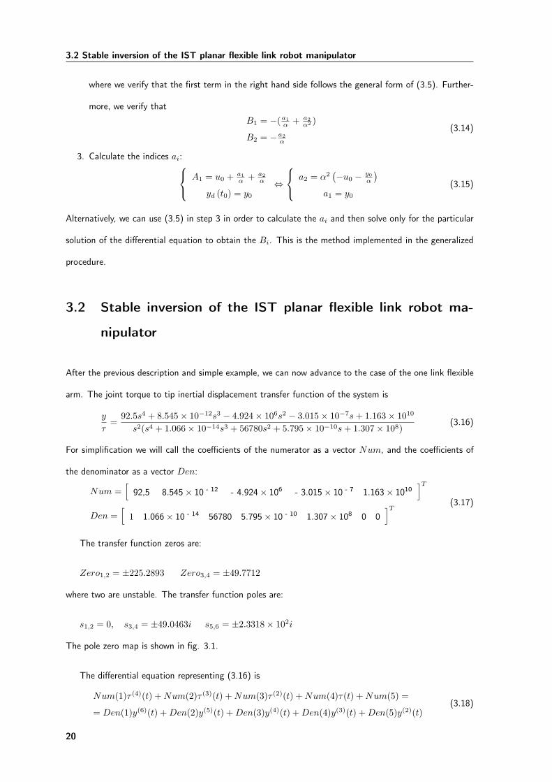
3.9 Simulation tracking error for an external input torque (Amplitude 0.002Nm) . . . . . . . 27
3.10 Simulated close-loop torque with an external input torque (Amplitude 0.1Nm) . . . . . . 27
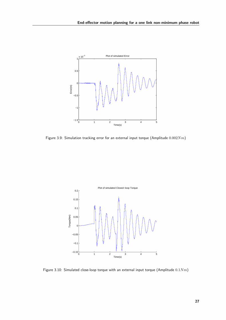
3.11 Simulation output with an external input torque (Amplitude 0.1Nm) . . . . . . . . . . . 28
3.12 Simulation tracking error for an external input torque (Amplitude 0.1Nm) . . . . . . . . . 28
ix
LIST OF FIGURES
3.13 Simulated close-loop torque with noise . . . . . . . . . . . . . . . . . . . . . . . . . . . . 29
3.14 Simulation output with noise . . . . . . . . . . . . . . . . . . . . . . . . . . . . . . . . . 29
3.15 Simulation tracking error with noise . . . . . . . . . . . . . . . . . . . . . . . . . . . . . 30
3.16 Simulated close-loop torque with miscalculated zeros . . . . . . . . . . . . . . . . . . . . 30
3.17 Simulation output with miscalculated zeros . . . . . . . . . . . . . . . . . . . . . . . . . 31
3.18 Simulation tracking error with miscalculated zeros . . . . . . . . . . . . . . . . . . . . . . 31
3.19 Desired θ . . . . . . . . . . . . . . . . . . . . . . . . . . . . . . . . . . . . . . . . . . . . 33
3.20 PD controller . . . . . . . . . . . . . . . . . . . . . . . . . . . . . . . . . . . . . . . . . 34
3.21 Simulated output . . . . . . . . . . . . . . . . . . . . . . . . . . . . . . . . . . . . . . . 34
3.22 Simulated end-effector deformation . . . . . . . . . . . . . . . . . . . . . . . . . . . . . . 34
3.23 Simulated error . . . . . . . . . . . . . . . . . . . . . . . . . . . . . . . . . . . . . . . . 35
3.24 Simulated output with an external input torque (Amplitude 0.002Nm) . . . . . . . . . . . 35
3.25 Simulated close-loop torque with an external input torque (Amplitude 0.002Nm) . . . . . 36
3.26 Simulation tracking error for an external input torque (Amplitude 0.002Nm) . . . . . . . 36
3.27 Simulated output with an external input torque (Amplitude 0.1Nm) . . . . . . . . . . . . 37
3.28 Simulated close-loop torque with an external input torque (Amplitude 0.1Nm) . . . . . . 37
3.29 Simulation tracking error for an external input torque (Amplitude 0.1Nm) . . . . . . . . . 38
3.30 Simulated close-loop torque with noise . . . . . . . . . . . . . . . . . . . . . . . . . . . . 38
3.31 Simulation output with noise . . . . . . . . . . . . . . . . . . . . . . . . . . . . . . . . . 39
3.32 Simulation tracking error with noise . . . . . . . . . . . . . . . . . . . . . . . . . . . . . 39
3.33 location of zeros and poles in a closed loop form for miss calculation of transfer function . 40
3.34 Simulated closed-loop torque with miscalculated zeros . . . . . . . . . . . . . . . . . . . . 41
3.35 Simulation output with miscalculated zeros . . . . . . . . . . . . . . . . . . . . . . . . . 41
3.36 Simulation tracking error with miscalculated zeros . . . . . . . . . . . . . . . . . . . . . . 42
4.1 Controller block diagram . . . . . . . . . . . . . . . . . . . . . . . . . . . . . . . . . . . 45
x
LIST OF FIGURES
4.2 The path in x, y coordinates . . . . . . . . . . . . . . . . . . . . . . . . . . . . . . . . . 48
4.3 First Path - Evolution of the desired output versus the path variable . . . . . . . . . . . . 49
4.4 First Path - Simulation tracking error . . . . . . . . . . . . . . . . . . . . . . . . . . . . 50
4.5 First Path - Deformation of the end-effector . . . . . . . . . . . . . . . . . . . . . . . . . 50
4.6 First Path - Evolution of the desired path variable versus the real path variable . . . . . . 51
4.7 Second Path - Simulation velocity profile . . . . . . . . . . . . . . . . . . . . . . . . . . 51
4.8 Second Path - Simulation tracking error . . . . . . . . . . . . . . . . . . . . . . . . . . . 52
4.9 Second Path - Evolution of the desired path variable versus the real path variable . . . . . 53
4.10 Second Path - Deformation of the end-effector . . . . . . . . . . . . . . . . . . . . . . . 53
4.11 Second Path - Simulation velocity profile . . . . . . . . . . . . . . . . . . . . . . . . . . 54
4.12 Second Path - Deformation of the end-effector . . . . . . . . . . . . . . . . . . . . . . . 54
4.13 Second Path - Simulation tracking error . . . . . . . . . . . . . . . . . . . . . . . . . . . 54
4.14 First Path validation - Simulation input torque (White noise with the noise power of 0.1) . 55
4.15 First Path validation - Deformation of the end-effector (White noise with the noise power
of 0.1) . . . . . . . . . . . . . . . . . . . . . . . . . . . . . . . . . . . . . . . . . . . . . 56
4.16 First Path validation - Simulation output (White noise with the noise power of 0.1) . . . . 56
4.17 First Path validation - Simulation tracking error (White noise with the noise power of 0.1) 57
4.18 Second Path validation - Simulation tracking error (External step input torque with ampli-
tude of 1Nm) . . . . . . . . . . . . . . . . . . . . . . . . . . . . . . . . . . . . . . . . 57
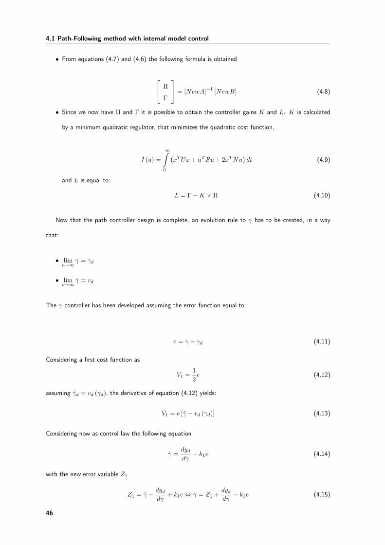
4.19 Second Path validation - Simulation input torque (External step input torque with amplitude
of 1Nm) . . . . . . . . . . . . . . . . . . . . . . . . . . . . . . . . . . . . . . . . . . . 58
4.20 Second Path validation - Deformation of the end-effector (External step input torque with
amplitude of 1Nm) . . . . . . . . . . . . . . . . . . . . . . . . . . . . . . . . . . . . . . 58
4.21 Second Path validation - Simulation Tracking error (White noise with the noise power of 1) 59
4.22 Second Path validation - Simulation input torque (Path properties: a1 = 1, a2 = 0.1 and
ms = 1) . . . . . . . . . . . . . . . . . . . . . . . . . . . . . . . . . . . . . . . . . . . . 59
4.23 Second Path validation - Deformation of the end-effector (Path properties: a1 = 1, a2 = 0.1
and ms = 1) . . . . . . . . . . . . . . . . . . . . . . . . . . . . . . . . . . . . . . . . . 60
xi
LIST OF FIGURES
4.24 Second Path validation - Simulation tracking error (Path properties: a1 = 1, a2 = 0.1 and
ms = 1) . . . . . . . . . . . . . . . . . . . . . . . . . . . . . . . . . . . . . . . . . . . . 60
4.25 Second Path validation - Evolution of the desired path variable versus the real path variable
(Path properties: a1 = 1, a2 = 0.1 and ms = 1) . . . . . . . . . . . . . . . . . . . . . . . 61
4.26 Second Path validation - Simulation output (Path properties: a1 = 1, a2 = 0.1 and ms = 1) 61
4.27 Second Path validation - Joint velocity versus error (Path properties: a1 = 1, a2 = 0.1 and
ms = 1) . . . . . . . . . . . . . . . . . . . . . . . . . . . . . . . . . . . . . . . . . . . . 62
4.28 Output values of flexible link identification . . . . . . . . . . . . . . . . . . . . . . . . . . 68
4.29 Flexible link identification validation . . . . . . . . . . . . . . . . . . . . . . . . . . . . . 70
4.30 Flexible link identification error . . . . . . . . . . . . . . . . . . . . . . . . . . . . . . . . 70
5.1 Identification input . . . . . . . . . . . . . . . . . . . . . . . . . . . . . . . . . . . . . . 72
5.2 Identification output . . . . . . . . . . . . . . . . . . . . . . . . . . . . . . . . . . . . . . 72
5.3 Location of zeros and poles in a close loop form . . . . . . . . . . . . . . . . . . . . . . . 73
5.4 End-effector vibration at low average velocity . . . . . . . . . . . . . . . . . . . . . . . . 74
5.5 End-effector vibration at high average velocity . . . . . . . . . . . . . . . . . . . . . . . . 74
5.6 Input torque at low average velocity . . . . . . . . . . . . . . . . . . . . . . . . . . . . . 75
5.7 Input torque at high average velocity . . . . . . . . . . . . . . . . . . . . . . . . . . . . . 75
A.1 Interpretation of structural decomposition of a SISO system . . . . . . . . . . . . . . . . 86
xii

List of Tables
2.1 IST flexible robot manipulator characteristics . . . . . . . . . . . . . . . . . . . . . . . . 15
xiii

LIST OF TABLES
xiv

Chapter 1
Introduction
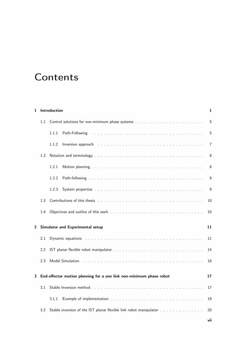
Robotics will have in the future an important role in our life (fig.1.1). Robot manipulator technology
is constantly improving, by increasing efficiency and becoming more human interactive [1]. The way to
achieve the same performance in terms of speed, acceleration and operational load with less weight and
increased human interactivity, is with flexible manipulator robots, due to their light weight structures and
mechanical flexibility.
But what are flexible manipulators robots, and why do we call them that? Generally, flexible manipu-
lators robots are manipulators that have mechanical flexibility in their links and joints, which results in the
vibration or oscillation of the end-effector either during the manipulator’s motion or immediately after it
stops. This behavior reduces the position precision, but on the other hand one can achieve higher velocities
due to the lower inertia and mass.
Flexibility can appear due to two factors: high accelerations in the motion or long and slender links
of the manipulators. Therefore, flexibility is a result of the demand for the manipulator operation. If the
manipulator operates at high acceleration, it may become flexible. If the manipulator operates in small
spaces, like surgical robots, it may need to be flexible. If the manipulator has to be light, because of
transportation demands for example, the use of small quantities of material or light materials results in
flexible structures.
To solve the problems resulting of structural flexibility, and have a satisfactory precision in the positioning
of the end-effector, industrial robot manipulators are built with a rigid structure. Such rigid structures are
1

Figure 1.1: Graph depicting the number of manuscripts indexed per year in a PubMed search containing
the words robot or robotic
achieved by using heavy and stiff designs, that increase the weight, therefore increasing the consumption
of energy during motion.
As interesting as flexible robots may seem for robotic surgery, the existing solutions are rigid. Active
(rigid) robotic devices, in which pre-programmed data and computer-generated algorithms function without
real-time operator input, were the first robots to be used in live surgical applications.
In 1985 [1], the first surgical application of industrial robotic technology was described when an indus-
trial robotic arm was modified to perform a stereotactic brain biopsy with 0.05 mm accuracy. This served
as the prototype for Neuromate (Integrated Surgical Systems, Sacramento, CA, USA) which received Food
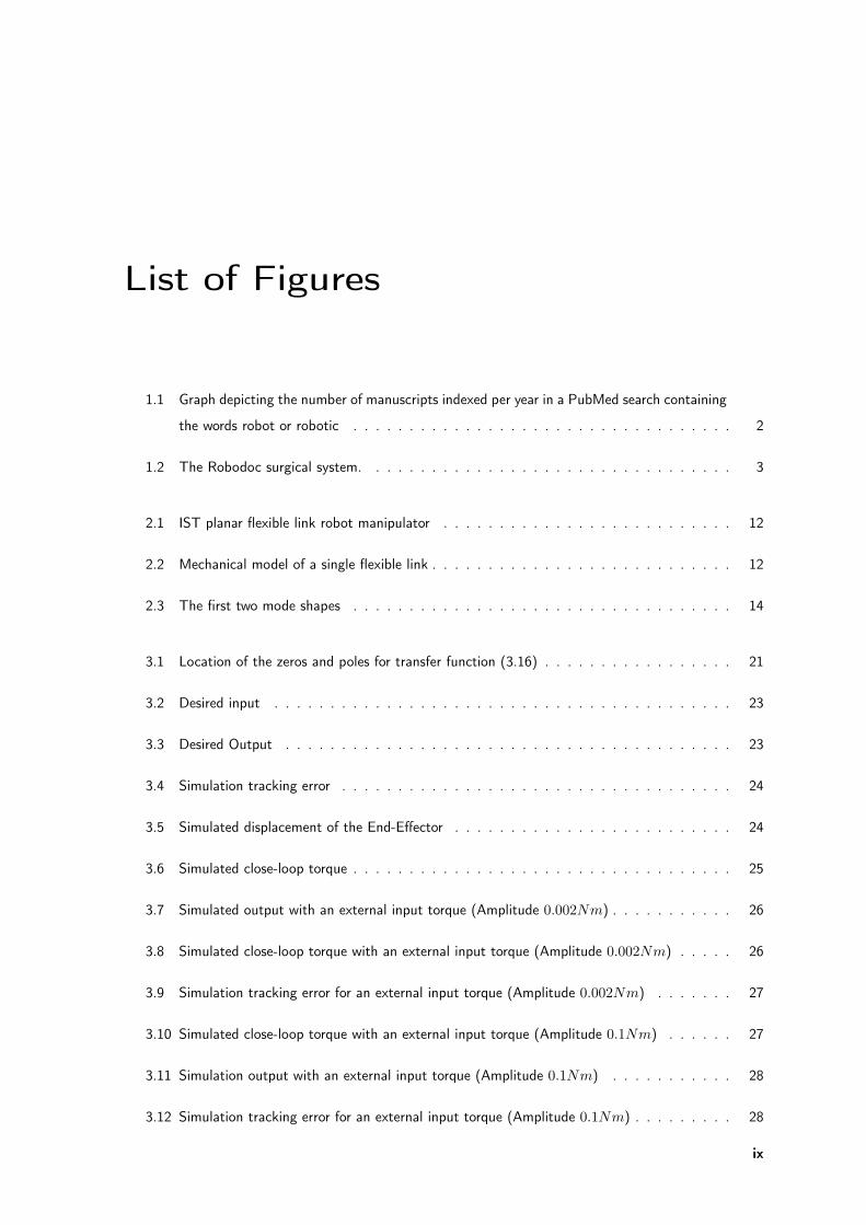
and Drug Administration (FDA) approval in 1999. Meanwhile, for orthopedics, in 1992, the Robodoc
(Integrated Surgical Systems) was introduced for use in hip replacement surgery (fig. 1.2). The Robodoc
is a computer-guided mill used to core the femoral head to receive a hip replacement prosthesis. Clinical
trials demonstrate greater accuracy comparing the well drilled by the Robodoc to conventional techniques.
Whereas the Robodoc has been used in thousands of patients in Europe, it has not yet received FDA
approval in the United States because of concerns regarding complication rates. Similar devices have been
2

Introduction
Figure 1.2: The Robodoc surgical system.
designed for use in knee replacement and temporal bone surgery, notably the Acrobot (The Acrobot Com-
pany, Ltd., London, UK) and the RX-130 robot (Staubli Unimation Inc., Faverges, France), respectively.
Neither device has yet completed clinical testing nor received FDA approval [1].
The dynamics equations of flexible manipulator robots are significantly more complex than those of
rigid robots due to the link’s flexibility. Flexibility yields a robot model with infinite degrees of freedom,
which must be truncated to a finite number.
There are three principal objectives in the control of the flexible robot arms:
• O1 - Point to point motion of the end-effector.
• O2 - Trajectory tracking in the joint space (tracking of a desired angular trajectory).
• O3 - Trajectory tracking in the operational space (tracking of a desired end-effector trajectory).
The control of the motion of flexible manipulators is one of the areas under great investigation in
robotics. In rigid manipulator robots, the control task is less complicated, since one achieves tip position
by controlling the joint angles. This is known as dead-reckoning, as this kind of control approach does
not contemplate feedback of the position of the end-effector. For flexible robots, there is the need to use
a controller designed to damp out the oscillations at the tip that appear during motion. In this project
3

we will discuss two methods to solve this problem. They are path-following [2], [3], [4], [5] and reference
tracking [6], [7], [8], [9].
4

Introduction
1.1 Control solutions for non-minimum phase systems
Due to the elastic deflection of a flexible beam, its linearized model possesses one real zero per vibration
mode in the right half complex plane. As is well known, unstable zero dynamics results in limitations on
the achievable performance and tracking capabilities. Dačic [5] presented three distinct approaches for
tracking in the presence of unstable zeros dynamics. He refered to them as: the Internal Model approach,
the Flatness approach and the Inversion approach. In this report we will focus on the internal model
approach and the inversion approach.
1.1.1 Path-Following
A path-following problem is first considered in robotics literature in [10]. The objective is to control a robot
using limited torques to move along a pre-arranged path in minimal time. Hauser and Hindman [11] started
a new path-following methodology, where the main objective, is to determine on-line a desirable velocity
profile along the path. They introduced a state path-following problem, where the path is specified for
each state variable of the system. Encarnação and Pascoal [12] proposed a different kind of path-following,
called output path-following, where the path is defined only for the system output. This report follows
this line of work, as in Aguiar [4], [2], [3] and Dačic [5]. In these works the path-following problem is
defined as a combination of two tasks: geometric and dynamic. Then, it is shown that it is possible to
construct feedback laws that can achieve an arbitrarily small L2 norm of the path-following error. This
property highlights the difference between path-following and reference tracking, where a fundamental
limitation exists in terms of a lower bound on the L2 norm of the tracking error imposed by the unstable
zero dynamics.
One of the major problems with non-minimum phase systems is to design control laws in order to
drive the output to reach and follow a geometric reference (path). Another problem is to compel the
system to follow the geometric reference and satisfy some additional dynamic specifications (as speed,
acceleration...). Since the limitations introduced by unstable zeros are structural, they cannot be avoided
without changing the system structure or reformulating the tracking problem. One of the reformulation
possibilities is to select a new output in which the zero dynamics become stable (change the output from
the end-effector to the hub rotation).
5
1.1 Control solutions for non-minimum phase systems
One approach to the path-following problem is shown in the work by Aguiar et al. [3] and [2], where
the authors introduce a new path variable γ, in order to suppress the time dependence of the motion.
In Dačic [5], an intuitive description is given to the problem. In his interpretation of path-following, a
fictitious object called the leader, is introduced. The leader moves along the path, and its current position
at the time t is γ(t). The main objective of the path-following control theory is to steer a physical object,
called the follower, to converge to the leader geometric path. The secondary objective is to ensure that the
object’s motion along the path satisfies a given dynamic specification.To assure this dynamic specification,
it is required to design a timing law for γ. This is a feedback law for the leader, which ensures that its
motion asymptotically satisfies the dynamics specification. We can assume that reference tracking is a
special case of path following, where the timing law γ(t) is pre-determinated.
Internal model approach
The goal of the internal model approach is to design control laws that are capable of driving an object (such
as a robot arm, ship or aircraft) to reach and follow a geometric path, and force the object to satisfy some
additional dynamic specification. This dynamic specification can be represented as outputs of a neutral
stable system, called exosystem. In Aguiar et al. [3] and [2], it was demonstrated that it is possible to
secure asymptotic convergence of the tracking error to zero. Since this approach is the one that originates
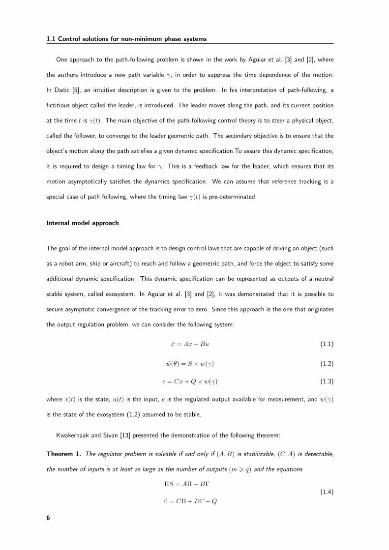
the output regulation problem, we can consider the following system:
x = Ax+Bu (1.1)
w(θ) = S × w(γ) (1.2)
e = Cx+Q× w(γ) (1.3)
where x(t) is the state, u(t) is the input, e is the regulated output available for measurement, and w(γ)
is the state of the exosystem (1.2) assumed to be stable.
Kwakernaak and Sivan [13] presented the demonstration of the following theorem:
Theorem 1. The regulator problem is solvable if and only if (A,B) is stabilizable, (C,A) is detectable,
the number of inputs is at least as large as the number of outputs (m > q) and the equations
ΠS = AΠ +BΓ
0 = CΠ +DΓ−Q(1.4)
6

Introduction
have solution for matrices Π and Γ.
It can also be shown that the last condition on Theorem 1 is equivalent to requiring that the eigenvalues
of the matrix S differ from the transmission zeros of (1.1). But the internal model approach does not avoid
the performance limitations due to unstable zero dynamics. In recent studies Aguiar et al. [3], [2] and [4]
has presented a solution, where this limitation can be avoided by the combination of the internal model
approach and the path-following. Their methodology consists in replacing the variable t in the geometric
path yd, by a path variable γ and then selecting a timing law to it. In this way, the variable γ is treated
as an additional control variable. Considering the new variable γ, it is possible to achieve an L2 norm of
the path-following error relatively small.
1.1.2 Inversion approach
The main idea of the inversion approach is to obtain a stable reference in order to acquire a finite smooth
control torque, that implies an exact reproduction of the computed trajectory, by using a simple input-
output inversion technique applied to our non-minimum phase system. Benosman and Le Vey [6], [7], [8]
and [9] presented a methodology to obtain a stable inversion via output planing of a single-input-single-
output (SISO) non-minimum phase system.
End-effector motion planning
One technique to reduce all the undesired behavior characteristics (such as vibration of the end-effector)
of a flexible robot, is to calculate the end-effector motion in such a way not to disturb the unstable zeros
of the system. Much work has been dedicated in the past two decades to the control of the flexible arm
models, and much of those works have yielded good results for the first two objectives described in O1 and
O2.
Benosman and Le Vey [6] made a profound analysis about stable inversion of a SISO non-minimum
phase linear system. Instead of searching for proper initial conditions associated to a given desired output,
this approach, consists in a search for a proper output, associated to the desired initial conditions. This
output is planned in a way that it is possible to cancel all the effects of the unstable zeros.
7
1.2 Notation and terminology
After knowing the required output, it is possible to estimate the capable input to obtain the desired
results. This methodology addresses the problem of planning a target tip trajectory, leading to a finite
smooth control torque that implies an exact reproduction of the computed trajectory, by using a simple
input-output inversion technique. Just as other common methodologies, the result of this methodology is
presented on an open loop control torque in the time domain.
1.2 Notation and terminology
This report follows a certain general notation and terminology, excepting in some particular examples,
where new auxiliary variables appear. Their meaning will then be described.
Time is always denoted by t. The particular time events, as final time and initial time are refered as tf
and ti respectively.
When a given function is i-times differentiable, appears f (i) for its ith time derivative, f (i) , dif(t)dti .
Identity matrix of dimension n is defined by In. The ith vector element is defined by V (i). The matrix
elements are represented with Aij , since they have two entries (ith row and jth column).
1.2.1 Motion planning
In chapter 3.1 we present some polynomial manipulations, where:
• Ai corresponds to the ith index of the polynomial representation of the stable and unstable transient
solution.
• Aist corresponds to the ith index of the polynomial representation of the stable transient solution.
• Bi correspond to the ith index of the polynomial representation of the particular solution.
The parameter α represents the system zeros, and αist correspond to the ith stable zero. The variables
Kp and Kv represent the PD controller proportional and derivative gain respectively.
8
Introduction
1.2.2 Path-following
Like in the literature, the system state space matrices are commonly represented by A,B,C,D. In path-
following methodology the leader is represented by the letter w, and the path-variable is represented by γ.
The variables K and L belong to the path-following controller. K is the gain vector obtained by the
LQR method, and L is the leader gain matrix.
Kron(X,Y ) is the Kronecker tensor product of X and Y representation. The result is a large matrix
formed by taking all possible products between the elements of X and those of Y . For example:
If X is a 2 by 3 matrix and Y is of any dimension, then Kron(X,Y ) is: X(1,1) × Y X(1,2) × Y X(1,3) × Y
X(2,1) × Y X(2,2) × Y X(3,1) × Y
(1.5)
1.2.3 System properties
The physical system properties are defined as:
• ω: frequency.
• τ : input torque.
• r: hub radius.
• Ih: hub inertia.
• Ib flexible beam inertia.
• l: flexible link length.
• υ(x): flexible link displacement at distance x from the base of the link.
• θ: Hub rotation angle.
• η: flexible link modal amplitude.
• φ: modal function.
9

1.3 Contributions of this thesis
1.3 Contributions of this thesis
This thesis is a general analysis approach to the flexible manipulator robot control problem. It compares
motion-planning and path-following control methodologies for the IST planar flexible manipulator robot.
It presents simulation and experimental results of the studied methodologies.
There are two innovative contributions of this thesis. First, in terms of reference planing, we present a
modification of the original approach in order to overcome joint friction. We introduce a joint controller
modifying the input from torque to joint angle. Second, to the knowledge of the author, this works presents
the first attempt to apply a path-following controller to flexible link manipulators.
1.4 Objectives and outline of this work
This thesis has as primary objective, the control of the position of the end-effector of a flexible robot with
a significant precision, assuming a path, from point one to point two, driven at variable speeds profile. To
this end, this thesis is composed of the following chapters :
Chapter 1: Introduction to the problem at hand.
Chapter 2: Overview of the modeling and experimental setup. The IST planar flexible manipulator
robot is presented, its dynamics equations and properties.
Chapter 3: Trajectory-planning control methodology. This methodology allows for computing a path,
leading to a feedforward torque, producing an exact reproduction of the path.
Chapter 4: Path-following control methodology, which allows us to control the non-minimum phase
system with a closed-loop form controller.
Chapter 5: Experimental results, obtained with end-effector motion planing
Chapter 6: Conclusions, summary of the work and recommendations for future work.
10

Chapter 2
Simulator and Experimental setup
In this chapter, the mathematical equations and a brief overview of the IST planar flexible robot manipulator
will be presented.
2.1 Dynamic equations
In Martins [14] two experimental robotic setups are presented. One for planar experiments, and another
for general three dimensional experiments. The work presented here refers to the planar IST flexible
manipulator, namely its flexible link, fig. 2.1. This robot has been studied in [15], [16] and [17] where it
is widely described.
The flexible link is clamped to a rigid hub with a moment of inertia (IH), radius (r) and an input
torque (τ). Considering linear displacements, the position of the link located at the distance x from the
frame origin, in the OX direction, relative to the {O0, X0, Y0, Z0, } (inertial), reference frame is given by
(fig. 2.2):
~p (x, t) = [x cos θ (t)− ν(x, t) sin θ (t)] e1 + [x sin θ (t)− ν(x, t) cos θ (t)] e2 (2.1)
where e1, e2 and e3 are the unit vectors along the X0, Y0 and Z0 axes respectively. The velocity of the
same infinitesimal element is accordingly given by
~p (x, t) =[−(xθ + ν
)sin (θ)− νθ cos (θ)
]e1 +
[(xθ + ν
)cos (θ)− νθ sin (θ)
]e2 (2.2)
11

2.1 Dynamic equations
Figure 2.1: IST planar flexible link robot manipulator
Figure 2.2: Mechanical model of a single flexible link
The kinetic energy of the system can deduced as [16]
T =12
(IH + Ib) θ2 +12
r+L∫r
ρ(ν2 + 2νxθ
)dx (2.3)
and the elastic potential energy of the beam as
V =12
r+l∫r
EI
(∂2ν
∂x2
)2
dx (2.4)
Martins et al. [16] also describes how to obtain the discrete ordinary differential equations of the current
system as
Mq +Kq = T (2.5)
12

Simulator and Experimental setup
Where M is the system inertia matrix, K is the system stiffness matrix, T is the vector of external torques
and q is the vector of generalized coordinates.
q = [θ η1 η2 . . . ηk]T
T = [τ 0 0 . . . 0]T(2.6)
Here, ηi is the modal amplitude of the ith mode considering the assumed modes discretization procedure,
being k the total number of assumed modes. The mass matrix and the stiffness matrix are given by
M =
IH + Ib ρr+L∫r
xφ1 (x) dx ρr+L∫r
xφ2 (x) dx · · · ρr+L∫r
xφk (x) dx
ρr+L∫r
xφ1 (x) dx ρL 0 0 0
ρr+L∫r
xφ2 (x) dx 0 ρL 0 0
......
.... . .
...
ρr+L∫r
xφk (x) dx 0 0 0 ρL
(2.7)
K =
0 0 0 · · · 0
0 ρLω21 0 0 0
0 0 ρLω22 0 0
......
.... . .
...
0 0 0 0 ρLω2k
(2.8)
The inertial displacement at a distance x from the frame origin in the OX direction is given by
y (x, t) = x θ (t) + ν (x, t) (2.9)
Observing (2.9) we can verify that the total displacement is a function of the rigid body motion θ (t) and
the elastic deflection (displacement) ν (x, t), where this latter term is discretized as
ν(x, t) =k∑i=1
φi (x) ηi (t) (2.10)
φi (x) and ηi (t) represent the modal functions and modal amplitudes of the ith Hermite-cubic mode
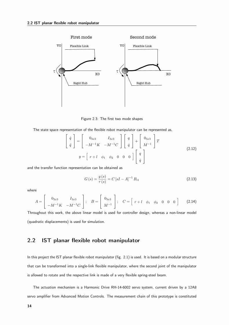
respectively. In this report we consider two Hermite-cubic modes. The modal functions are:
φ1 (x) = 3( xL
)2
− 2(xl
)3
φ2 (x) =( xL
)2
−(xl
)3
φ (x) =[φ1 (x) φ2 (x)
] (2.11)
where the modes shape are presented in fig. 2.3.
13
2.2 IST planar flexible robot manipulator
First mode
Y0
X0!
Flexible Link
Rigid Hub
Second mode
Y0
X0!
Flexible Link
Rigid Hub
Figure 2.3: The first two mode shapes
The state space representation of the flexible robot manipulator can be represented as, q
q
=
03x3 I3x3
−M−1K −M−1C
q
q
+
03x3
M−1
Ty =
[r + l φ1 φ2 0 0 0
] q
q
(2.12)
and the transfer function representation can be obtained as
G (s) =y (s)τ (s)
= C [sI −A]−1Bi1 (2.13)
where
A =
03x3 I3x3
−M−1K −M−1C
; B =
03x3
M−1
; C =[r + l φ1 φ2 0 0 0
](2.14)
Throughout this work, the above linear model is used for controller design, whereas a non-linear model
(quadratic displacements) is used for simulation.
2.2 IST planar flexible robot manipulator
In this project the IST planar flexible robot manipulator (fig. 2.1) is used. It is based on a modular structure
that can be transformed into a single-link flexible manipulator, where the second joint of the manipulator
is allowed to rotate and the respective link is made of a very flexible spring-steel beam.
The actuation mechanism is a Harmonic Drive RH-14-6002 servo system, current driven by a 12A8
servo amplifier from Advanced Motion Controls. The measurement chain of this prototype is constituted
14
Simulator and Experimental setup
by an incremental encoder with 2000 pulses per revolution that measure the position of the joint, and
three Wheatstone bridges along the flexible arm, at 4.5cm, 18cm and 32cm from joint 2, to measure the
bending represented by variables ν′′(x1), ν
′′(x2) and ν
′′(x3) respectively. For the purposes of this work
only the first two were used. It was verified that for the smooth trajectories tested here the first two modes
suffice. In table 2.1 the most important properties of the IST planar manipulator are presented.
IST Manipulator physical properties
Beam length (l) 0.5m
Beam width 0.001m
Beam height 0.02m
Mass density (ρ) 7850 Kg/m3
Beam Young modulus (E) 209× 109 Pa
Hub radius (r) 0.075m
Natural clambed-free beam frequencies
ω1 20.95 rad/s (3.33Hz)
ω2 131.28 rad/s (20.89Hz)
ω3 367.6 rad/s (58.5Hz)
Table 2.1: IST flexible robot manipulator characteristics
To integrate the various components of the experimental setup, and implement the real time control of
the robot, the MATLAB toolbox xPC Target was used. The xPC Target, in its basic configuration, needs
two computers: the Host computer, where the control programs are created, and the Target computer that
is responsible for the real time computation. The connections to the robot are performed through an I/O
Servotogo board, which drives are created as a library for MATLAB.
In the Host computer, the control programs are created in the Simulink environment of MATLAB that
are compiled in C code, creating an executable that is sent to the Target computer in which the application
runs in real time. In this configuration, the Target computer needs a processor and a RAM memory with
enough capacity to run the applications only, since an operating system isn’t necessary. The programs used
in this work were created in MATLAB version 7.0.1 which has the Simulink version 6.1 and the version 2.6
of the xPC Target toolbox. The Target computer has a Pentium MMX processor at 233MHz and 28MB
of RAM memory.
15

2.3 Model Simulation
2.3 Model Simulation
For model simulation, a Matlab toolbox called MECANISMO, has been used. This toolbox was developed
in Martins [14], it works seamlessly with other Matlab tools, and has been coded with special attention
to its usage in a real time framework. The modules of MECANISMO, along with other tools available in
Simulink, especially the numerical integrators, allow for simulation in free, constrained and impact motion
of flexible manipulators. A quadratic model has been built with MECANISMO for model simulation.
16
Chapter 3
End-effector motion planning for a
one link non-minimum phase robot
The objective of this study is to stabilize a single-input single-output non-minimum phase system. In this
study it is common to use a u as input, a y as output and an s as the Laplace transform variable.
3.1 Stable Inversion method
Consider u and y related by a given input-output equation
P (d
dt)u(t) = Q(
d
dt)y(t) (3.1)
Here, P and Q are polynomials in a differential operator d/dt, with degrees m and n respectively (m < n).
In a first analysis, due to the linear nature of equation (3.1), its solution is composed by two terms.
• The transient.
• The Steady-State.
Since the system has a non-minimum phase characteristic, the transient of the system’s inverse contains
divergent terms, resulting from the unstable zeros. So, in this case, one solution to the problem is to plan
the output trajectory in such a way that the undesirable response of the system input is cancelled. To
17

3.1 Stable Inversion method
cancel these undesired terms, a polynomial in time form for the output trajectory is considered
yd =p∑i=1
aiti−1 (3.2)
where the degree of the polynomial form p depends on the number of output initial and final constraints,
as well as the number of unstable zeros associated to equation (3.1).
The input in equation (3.1) may be written as
u(t) = ut(t) + up(t) (3.3)
where ut is the transient solution and up is the particular solution of the inverse system. The transient
solution can be represented by:
ut(t) =m∑i=1
Ai(ai, t0, u0, u(1)0 , ..., u
(n−1)0 )eri,t (3.4)
where the ri are all the roots of the characteristic equation of the inverse problem. The Ai are linear
functions of the ai coefficients and all initial conditions. It is shown in [6] that their general expression is
Ai = u0 +p∑j=1
aj
zeroji(3.5)
Furthermore, the particular solution can be represented by:
up(t) =p∑i=1
Bi(ai)ti−1 (3.6)
To cancel the effect of the unstable zeros on the transient solution (3.4) (all the zeros in the right half
plane or pure imaginary zeros), the Ai associated with the unstable zeros must be equal to zero
Ai(ai, t0, u0, u(1)0 , ..., u
(n−1)0 ) = 0 (3.7)
With this constraint in the linear system, we can obtain the output coefficients (ai). Adding the final and
initial constraints, this leads to the linear system:Ai(ai, t0, u0, u
(1)0 , ..., u
(n−1)0 ) = 0
yid(t0) = initial conditions
yid(tf ) = final conditions
(3.8)
where i is the highest order for the specified output derivatives. From equation (3.8) we have the coefficients
ai and the necessary output to cancel the unstable zeros. So, the result of the remaining Ai is known. To
18
End-effector motion planning for a one link non-minimum phase robot
complete the desired input, u(t), it is only necessary to obtain the particular input solution (3.6). The Bi
elements are obtained as linear functions of the output coefficients ai, through substitution of equation
(3.4) into the differential equation (3.1).
At this point, all necessary elements to obtain the desired input in an open loop form are:
uol =p∑i=1
Bi(ai)ti−1 +m∑i=1
Aist(ai, t0, u0, u(1)0 , ..., u
(n−1)0 )erist,ti (3.9)
where rist and Aist, are the stable zeros from the corresponding Ai terms. In a final approach to the
problem, it is recommended to close the loop around the joint angle in order to gain some robustness. The
final control law in a closed-loop form is:
ucl(t) = uol(t) +K
eθ
e1θ...
ev−1θ
(3.10)
where the error is eθ(t) = θd(t)− θ(t)
3.1.1 Example of implementation
As an introduction to the problem, let us consider a simple example. Consider the following input-output
equation:
u(t)(1) − αu(t) = y(t), (3.11)
where α is the unstable zero. In order to cancel the undesired non-minimum phase characteristics, we
calculate the input as in (3.9).
1. To obtain the output (3.2) which cancels all unstable zeros, we write:
yd(t) = a1 + a2t, (3.12)
where p = 2, since we have an unstable zero in s = α, and an initial output value y(t = 0) = y0.
2. Substituting (3.12) into (3.11) and solving for u, we obtain:
u(t) = (u0 +a1
α+a2
α2)eαt − (
a1
α+a2
α2)− a2
αt (3.13)
19
3.2 Stable inversion of the IST planar flexible link robot manipulator
where we verify that the first term in the right hand side follows the general form of (3.5). Further-
more, we verify that
B1 = −(a1α + a2
α2 )
B2 = −a2α
(3.14)
3. Calculate the indices ai: A1 = u0 + a1α + a2
α
yd (t0) = y0⇔
a2 = α2(−u0 − y0
α
)a1 = y0
(3.15)
Alternatively, we can use (3.5) in step 3 in order to calculate the ai and then solve only for the particular
solution of the differential equation to obtain the Bi. This is the method implemented in the generalized
procedure.
3.2 Stable inversion of the IST planar flexible link robot ma-
nipulator
After the previous description and simple example, we can now advance to the case of the one link flexible
arm. The joint torque to tip inertial displacement transfer function of the system is
y
τ=
92.5s4 + 8.545× 10⁻¹²s3 − 4.924× 10⁶s2 − 3.015× 10⁻⁷s+ 1.163× 10¹⁰
s2(s4 + 1.066× 10⁻¹⁴s3 + 56780s2 + 5.795× 10⁻¹⁰s+ 1.307× 10⁸)(3.16)
For simplification we will call the coefficients of the numerator as a vector Num, and the coefficients of
the denominator as a vector Den:
Num =[92,5 8.545× 10 - 12 - 4.924× 10⁶ - 3.015× 10 - 7 1.163× 10¹⁰
]TDen =
[1 1.066× 10 - 14 56780 5.795× 10 - 10 1.307× 10⁸ 0 0
]T (3.17)
The transfer function zeros are:
Zero1,2 = ±225.2893 Zero3,4 = ±49.7712
where two are unstable. The transfer function poles are:
s1,2 = 0, s3,4 = ±49.0463i s5,6 = ±2.3318× 10²i
The pole zero map is shown in fig. 3.1.
The differential equation representing (3.16) is
Num(1)τ (4)(t) +Num(2)τ (3)(t) +Num(3)τ (2)(t) +Num(4)τ(t) +Num(5) =
= Den(1)y(6)(t) +Den(2)y(5)(t) +Den(3)y(4)(t) +Den(4)y(3)(t) +Den(5)y(2)(t)(3.18)
20

End-effector motion planning for a one link non-minimum phase robot
−250 −150 −50 50 150 250−250
−150
−50
50
150
250
Pole−Zero Map
Real Axis
Imag
inar
y A
xis
Figure 3.1: Location of the zeros and poles for transfer function (3.16)
associated to the initial conditions:
τ(0) = τ (1)(0) = τ (2)(0) = τ (3)(0) = 0
y(0) = y(1)(0) = y(2)(0) = y(3)(0) = y(4)(0) = y(5)(0) = 0
As shown previously, the obtained input-output equation can be associated to any initial conditions. For
this particular case, they have been assumed to be equal to zero.
The output that will cancel the unstable zero dynamics is now found. From (3.2), with p = 12 (2
unstable zeros plus 4 initial conditions on τ plus 6 initial conditions on y) we have
yd = a1 + a2 × t+ a3 × t2 + a4 × t3 + a5 × t4+
+a6 × t5 + a7 × t6 + a8 × t7 + a9 × t8+
+a10 × t9 + a11 × t10 + a12 × t11(3.19)
yd must satisfy 12 constraints:
• The indices Ai corresponding to the unstable zeros
• Initial and final conditions.
21

3.2 Stable inversion of the IST planar flexible link robot manipulator
A1 = τ0 + a1Zero1
+ a2Zero21
+ a3Zero31
+ a4Zero41
+ a5Zero51
+ a6Zero61
+ a7Zero71
+a8
Zero81+ a9
Zero91+ a10
Zero101+ a11
Zero111+ a12
Zero121= 0
A3 = τ0 + a1Zero3
+ a2Zero23
+ a3Zero33
+ a4Zero43
+ a5Zero53
+ a6Zero63
+ a7Zero73
+a8
Zero83+ a9
Zero93+ a10
Zero103+ a11
Zero113+ a12
Zero123= 0
yi(0) = 0 i ∈ {0, 1, 2, 3}
y(tf ) = yf
yi(tf ) = 0 i ∈ {1, 2, 3, 4, 5}
(3.20)
Note that these conditions were chosen to force the desired torque to be symmetric. The desired ai
coefficients are then directly obtained, solving the linear system above. In this way it’s possible to calculate
the transient solution of the system (3.4).
The next step is to obtain the particular solution of the system (3.6). The coefficients Bi are obtained
as linear functions of the output coefficients ai, substituting (3.6) and (3.19) into (3.18) yields.
For the constant values:
720a7Den(1) + 120a6Den(2) + 24a5Den(3)+
+6a4Den(4) + 3a3Den(5) = 24Num(1)B5+
+6Num(2)B4 + 2Num(3)B3 +Num(4)B2 +Num(5)B1
For the coefficients of t:
5040a8Den(1) + 720a7Den(2) + 120a6Den(3) + 24a5
Den(4) + 6a4Den(5) = 120Num(1)B6 + 24Num(2)B5+
+6Num(3)B4 + 2Num(4)B3 +Num(5)B2
For the coefficients of t2:
20160a9Den(1) + 2520a8Den(2) + 360a7Den(3)+
+60a6Den(4) + 12a5Den(5) = 360Num(1)B7 + 60
Num(2)B6 + 12Num(3)B5 + 3Num(4)B4 +Num(5)B3
...
For the coefficients of t12:
Num(5)B12 = 0
Solving this system of linear equations, we obtain all indices Bi for the particular solution (3.6). The
resulting of desired output and input are shown in figs. 3.2 and 3.3.
As introduced in section 3.1, equation (3.10), in order to bring some robustness to this control, a
closed-loop form should be used. Two types of control were chosen.
22

End-effector motion planning for a one link non-minimum phase robot
0 0.5 1 1.5 2 2.5 3−0.015
−0.01
−0.005
0
0.005
0.01
0.015Plot of desired InPut
Time(s)
Tor
que(
Nm
)
Figure 3.2: Desired input
0 0.5 1 1.5 2 2.5 3−0.05
0
0.05
0.1
0.15
0.2
0.25
0.3
0.35Plot of desired OutPut
Time(s)
Y(m
)
Figure 3.3: Desired Output
1. A partial state feedback, based on the joint position and velocity variables.
Tcl = Tol +Kp(θd(t)− θ(t)) +Kv(θd(t)− θ(t))
Kp > 0, Kv > 0
2. An open loop form where the input to the system is the angle of the joint.
3.3 Simulation Results
In this section we report some simulation results on the IST planar flexible manipulator shown in fig. 2.2.
23

3.3 Simulation Results
3.3.1 Control where the input is the torque
The method was applied for tf = 2.7s and yf = −0.35m (fig. 3.2 and fig. 3.3). The closed loop control
was obtained using Kp = 4 and Kv = 0.03.
0 1 2 3 4 5−3
−2
−1
0
1
2
3x 10
−5 Plot of simulated Error
Time(s)
Err
or(m
)
Figure 3.4: Simulation tracking error
0 0.5 1 1.5 2 2.5 3 3.5 4 4.5 5−1.5
−1
−0.5
0
0.5
1
1.5x 10
−3 End−effector vibration
Time(s)
End
−ef
fect
or v
ibra
tion
(m)
Figure 3.5: Simulated displacement of the End-Effector
In figs. 3.4 and 3.5 we present the simulation tracking error and the corresponding displacement of the
end-effector. After a brief analysis, we obtain the stationary error equal to 2.5× 10⁻⁷m, and the vibration
on the end effector equal to about 2 × 10⁻⁷m. Those are very small values compared to those obtained
during the path evolution. The minor residual oscillations (t > 2.5s) verified in fig. 3.4 is due to the fact
that the simulated model is quadratic in deformation [15], as explained in section 2.3.
24

End-effector motion planning for a one link non-minimum phase robot
0 0.5 1 1.5 2 2.5 3 3.5 4 4.5 5−0.015
−0.01
−0.005
0
0.005
0.01
0.015Torque in the close loop simulation
Time(s)
Inpu
t Tor
que(
Nm
)
Figure 3.6: Simulated close-loop torque
Fig. 3.6 presents the output torque of the close-loop form. Indiscernible in this figure, are the small
differences from the desired, due to the addition of the tracking error.
Validation
Hereafter the effects of exterior factors are simulated, such as noise, external torque input, and miss
calculation of the transfer function zeros.
Introducing an input torque starting at t = 1s and ending at t = 2.4s, with an amplitude 0.002Nm,
the following results were obtained. Analyzing fig. 3.7, fig. 3.8 and fig. 3.9 it is visible that the closed-
loop control is very robust on eliminating the unstable zeros effects, even when there is an external input
torque. Naturally there are some limitations. If the input torque is 10 times larger than the maximum
torque (0.1Nm), the controller will have some problems to achieve the desired results (figs. 3.10, 3.11
and 3.12).
25

3.3 Simulation Results
0 1 2 3 4 5−0.05
0
0.05
0.1
0.15
0.2
0.25
0.3
0.35
0.4Plot of simulated Y
Time(s)
Y(m
)
Figure 3.7: Simulated output with an external input torque (Amplitude 0.002Nm)
0 1 2 3 4 5−0.015
−0.01
−0.005
0
0.005
0.01
0.015Plot of simulated Closed−loop Torque
Time(s)
Tor
que(
Nm
)
Figure 3.8: Simulated close-loop torque with an external input torque (Amplitude 0.002Nm)
26
End-effector motion planning for a one link non-minimum phase robot
0 1 2 3 4 5−1.5
−1
−0.5
0
0.5
1x 10
−3 Plot of simulated Error
Time(s)
Err
or(m
)
Figure 3.9: Simulation tracking error for an external input torque (Amplitude 0.002Nm)
0 1 2 3 4 5−0.15
−0.1
−0.05
0
0.05
0.1
0.15
0.2Plot of simulated Closed−loop Torque
Time(s)
Tor
que(
Nm
)
Figure 3.10: Simulated close-loop torque with an external input torque (Amplitude 0.1Nm)
27
3.3 Simulation Results
0 1 2 3 4 5−0.05
0
0.05
0.1
0.15
0.2
0.25
0.3
0.35
0.4Plot of simulated Y
Time(s)
Y(m
)
Figure 3.11: Simulation output with an external input torque (Amplitude 0.1Nm)
0 1 2 3 4 5−0.06
−0.04
−0.02
0
0.02
0.04
0.06Plot of simulated Error
Time(s)
Err
or(m
)
Figure 3.12: Simulation tracking error for an external input torque (Amplitude 0.1Nm)
28
End-effector motion planning for a one link non-minimum phase robot
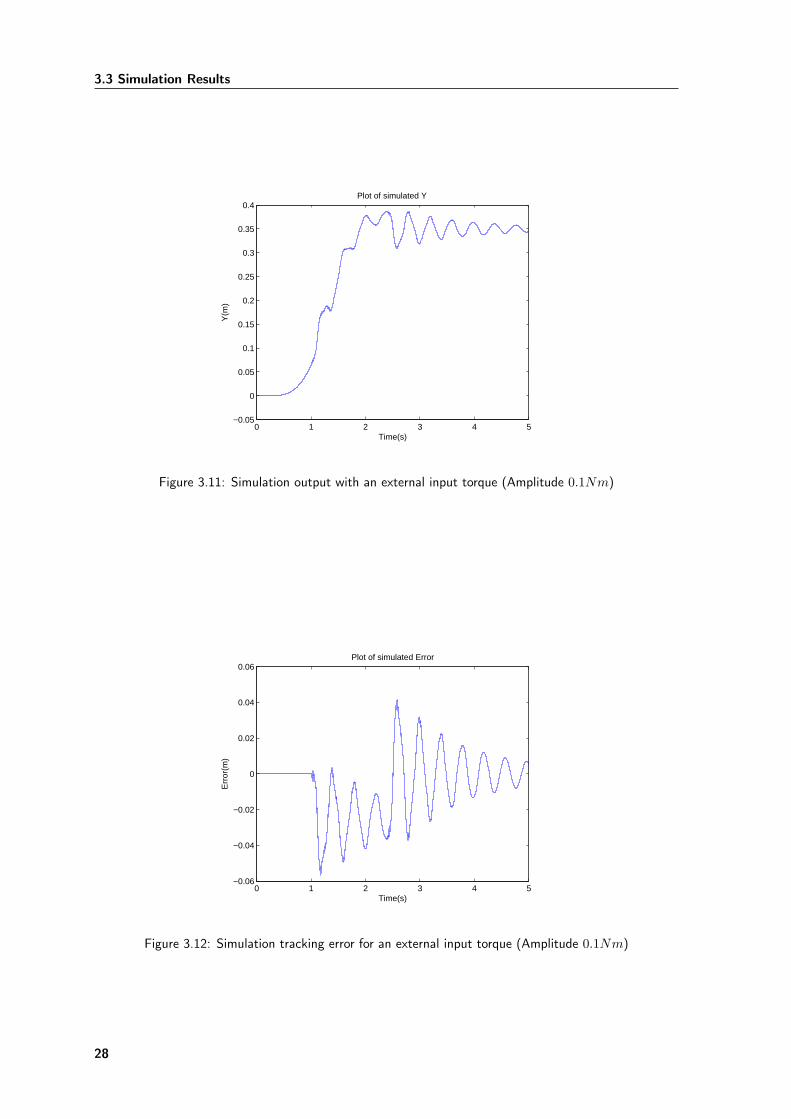
When analyzing the effect of noise in the system, a noise signal with 1% of the maximum standard
input value was introduced in the closed-loop input signal and in the output measurement. The results
are shown in figs. 3.13, 3.14 and 3.15. As expected, the noise affects the precision of the system, and
produces an undesired response of the closed-loop torque.
0 1 2 3 4 5−0.08
−0.06
−0.04
−0.02
0
0.02
0.04
0.06
0.08Plot of simulated Closed−loop Torque
Time(s)
Tor
que(
Nm
)
Figure 3.13: Simulated close-loop torque with noise
0 1 2 3 4 5−0.05
0
0.05
0.1
0.15
0.2
0.25
0.3
0.35
0.4Plot of simulated Y
Time(s)
Y(m
)
Figure 3.14: Simulation output with noise
29
3.3 Simulation Results
0 1 2 3 4 5−4
−2
0
2
4
6
8
10
12
14
16x 10
−3 Plot of simulated Error
Time(s)
Err
or(m
)
Figure 3.15: Simulation tracking error with noise
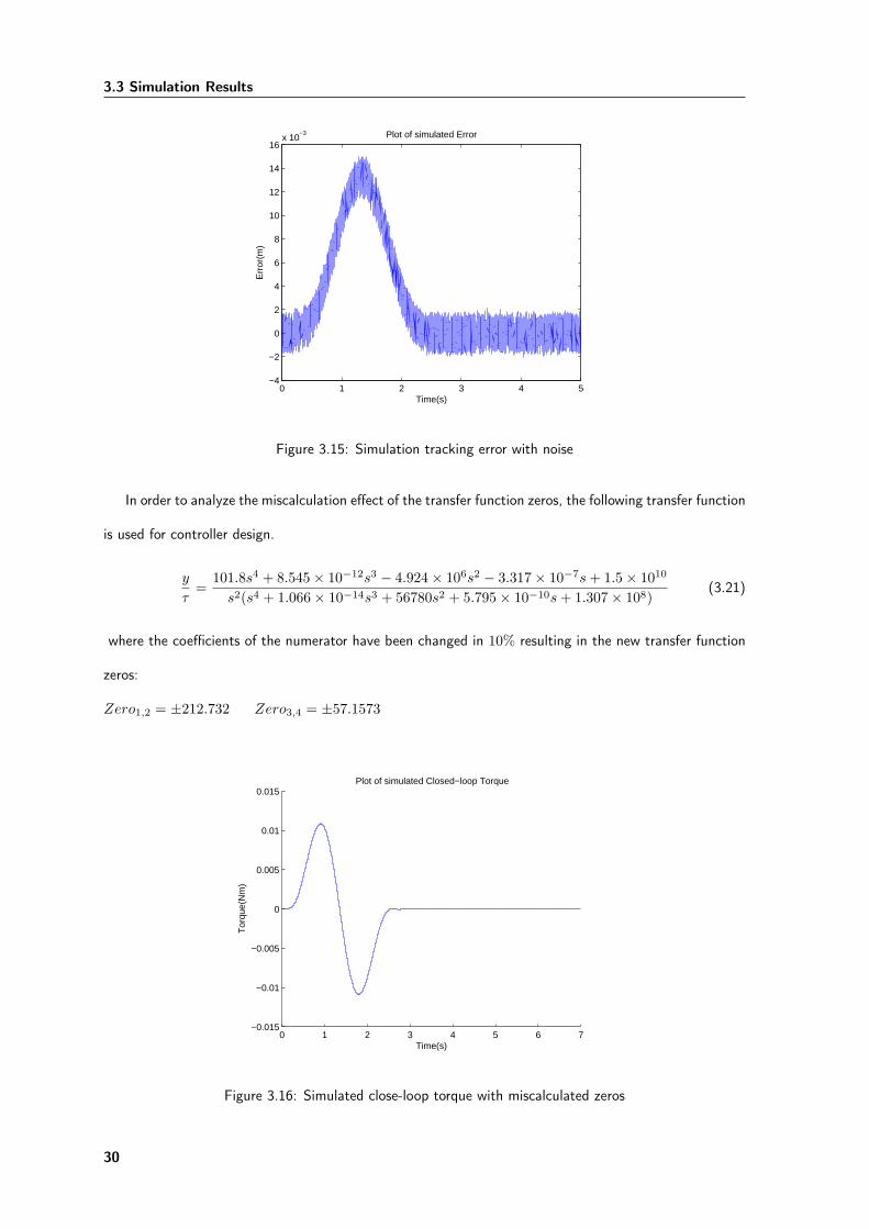
In order to analyze the miscalculation effect of the transfer function zeros, the following transfer function
is used for controller design.
y
τ=
101.8s4 + 8.545× 10⁻¹²s3 − 4.924× 10⁶s2 − 3.317× 10⁻⁷s+ 1.5× 10¹⁰
s2(s4 + 1.066× 10⁻¹⁴s3 + 56780s2 + 5.795× 10⁻¹⁰s+ 1.307× 10⁸)(3.21)
where the coefficients of the numerator have been changed in 10% resulting in the new transfer function
zeros:
Zero1,2 = ±212.732 Zero3,4 = ±57.1573
0 1 2 3 4 5 6 7−0.015
−0.01
−0.005
0
0.005
0.01
0.015Plot of simulated Closed−loop Torque
Time(s)
Tor
que(
Nm
)
Figure 3.16: Simulated close-loop torque with miscalculated zeros
30

End-effector motion planning for a one link non-minimum phase robot
0 1 2 3 4 5 6 7−0.05
0
0.05
0.1
0.15
0.2
0.25
0.3
0.35
0.4Plot of simulated Y
Time(s)
Y(m
)
Figure 3.17: Simulation output with miscalculated zeros
0 1 2 3 4 5 6 7−2
−1.5
−1
−0.5
0
0.5
1
1.5
2x 10
−3 Plot of simulated Error
Time(s)
Err
or(m
)
Figure 3.18: Simulation tracking error with miscalculated zeros
31

3.3 Simulation Results
Observing figs. 3.16 to 3.18, we can conclude that this miscalculation of the transfer function zeros
is not very relevant, since the calculation of the input torque is obtained in a way that doesn’t excite a
reasonable band of frequency. It is important to notice that the error shown in fig. 3.17 tends to a smaller
value than the obtained from fig. 3.4 due to the increase of the static gain, originated by the new transfer
function.
3.3.2 Control where the input of the system is the angle of the joint.
In this type of controller, the main idea is to make the system robust to external factors such as joint friction.
Instead of calculating the transfer function between the torque and the position of the end-effector, the
transfer function between the angle of the joint and the position of the end-effector has been calculated.
Considering the following control law
τ = kp (θr − θ)− kv θ (3.22)
associated to equation (3.16), we obtain the following transfer function
y
θ=
1330s4 + 1.398× 10⁻⁹s3 − 7.079× 10⁷s2 + 7.493× 10⁻⁵s+ 1.672× 10¹¹
s6 + 334.3s5 + 7.198× 10⁷s4 + 1.456× 10⁷s+ 7.925× 10⁸s2 + 6.393× 10⁹ + 2.907× 10¹¹
(3.23)
Calculating the desired angle in a way that the undesired transient response is eliminated, the following
curve is obtained (fig 3.19).
The joint controller is obtained in the following steps.
1. Calculate the second moment of inertia of the rigid system
I = JHub +m× (L
2)2 (3.24)
Where JHub is the second moment of inertia of the Hub and m and L are the mass and the length
of the flexible part respectively. For this system I = 0.006Kg/m2.
2. Now it’s possible to obtain the derivative part of the controller since:
θ
τ=
10.006× s
(3.25)
32

End-effector motion planning for a one link non-minimum phase robot
0 0.1 0.2 0.3 0.4 0.5 0.6 0.7 0.8 0.9 10
0.1
0.2
0.3
0.4
0.5
0.6
0.7Plot of desired θ
Time(s)
θ(ra
d)
Figure 3.19: Desired θ
which in closed loop becomes
Gclv =Kv
0.006× s+Kv(3.26)
where Kv is the gain of the derivative part.
3. The desired pole is:
P = − Kv
0.006× 2
4. The calculation of the proportional part of the controller is obtained by the following transfer function:
Gclp =Kp ×Kv
0.006× s2 +Kv × s+Kp ×Kv(3.27)
5. Solving two equations with two variables:
{Kp = −P2Kv = −0.0055× 2× P
(3.28)
where P is the position of our desired pole. (Note that P is always negative)
The following results were obtained using P = −50. Fig. 3.20 shows the representation on a block diagram
of the PD controller.
By observing figs. 3.21 to 3.23, we notice that the stationary error has been reduced to an insignificant
value. Using this controller the system has become more robust to external factors such as joint friction
as shown next, and reduces the residual vibration in the steady state.
33

3.3 Simulation Results
! +
-
-P/2
Kp+
-
System
"!#"$
!
-P*0.0055*2
Kv
τ
Figure 3.20: PD controller
0 1 2 3 4 5 6 7−0.1
0
0.1
0.2
0.3
0.4
0.5
0.6
0.7Plot of simulated Yreal
Time(s)
Yre
al(m
)
Figure 3.21: Simulated output
Figure 3.22: Simulated end-effector deformation
34

End-effector motion planning for a one link non-minimum phase robot
0 1 2 3 4 5 6 7−0.005
0
0.005
0.01
0.015
0.02
0.025
0.03
0.035Plot of simulated Error
Time(s)
Err
or(m
)
Figure 3.23: Simulated error
Validation
As in the previous validation, the effects of external factors, such as noise, external torque input, and miss
calculation of the transfer function zeros will be analyzed here.
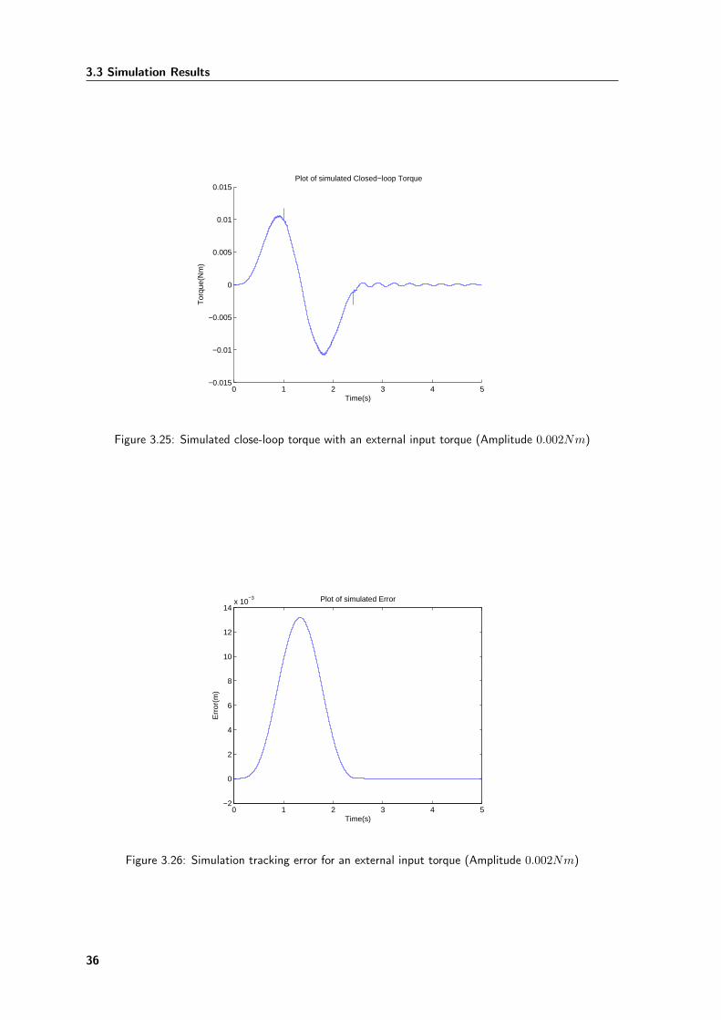
Introducing an input torque starting at t = 1s and ending at t = 2.4s, with an amplitude of 0.002N/m,
the obtained results are.
0 1 2 3 4 5−0.1
0
0.1
0.2
0.3
0.4
0.5
0.6
0.7Plot of simulated Y
Time(s)
Yre
al(m
)
Figure 3.24: Simulated output with an external input torque (Amplitude 0.002Nm)
Analyzing figs. from 3.24 to 3.26 it’s visible that this control is very robust on eliminating the effect
of the unstable zeros, even when there is an external input torque. The main difference between these
35
3.3 Simulation Results
0 1 2 3 4 5−0.015
−0.01
−0.005
0
0.005
0.01
0.015Plot of simulated Closed−loop Torque
Time(s)
Tor
que(
Nm
)
Figure 3.25: Simulated close-loop torque with an external input torque (Amplitude 0.002Nm)
0 1 2 3 4 5−2
0
2
4
6
8
10
12
14x 10
−3 Plot of simulated Error
Time(s)
Err
or(m
)
Figure 3.26: Simulation tracking error for an external input torque (Amplitude 0.002Nm)
36

End-effector motion planning for a one link non-minimum phase robot
controllers is when the undesired torque increases. Setting the perturbation torque to 0.1Nm, the following
results are achieved. Comparing figs. 3.27 to 3.29 with figs. 3.10 to 3.12, it’s clear that this controller has
become much more robust than the previous one. Also by analyzing fig. 3.28, it’s observable where the
external input was applied (t=1s and t=1.4s).
0 1 2 3 4 5−0.1
0
0.1
0.2
0.3
0.4
0.5
0.6
0.7Plot of simulated Y
Time(s)
Yre
al(m
)
Figure 3.27: Simulated output with an external input torque (Amplitude 0.1Nm)
0 1 2 3 4 5−0.2
−0.15
−0.1
−0.05
0
0.05
0.1
0.15Plot of simulated Closed−loop Torque
Time(s)
Tor
que(
Nm
)
Figure 3.28: Simulated close-loop torque with an external input torque (Amplitude 0.1Nm)
Analyzing now the effect of noise in this controller, we submit the system to the same noise tests as the
previous controller. The results in figs. 3.30, 3.31, 3.32 have been obtained. As in the previous controller,
it is clear that the effect of the noise isn’t significant to the output value.
37

3.3 Simulation Results
0 1 2 3 4 5−4
−2
0
2
4
6
8
10x 10
−3 Plot of simulated Error
Time(s)
Err
or(m
)
Figure 3.29: Simulation tracking error for an external input torque (Amplitude 0.1Nm)
0 1 2 3 4 5−0.08
−0.06
−0.04
−0.02
0
0.02
0.04
0.06
0.08Plot of simulated Closed−loop Torque
Time(s)
Tor
que(
Nm
)
Figure 3.30: Simulated close-loop torque with noise
38

End-effector motion planning for a one link non-minimum phase robot
0 1 2 3 4 5−0.05
0
0.05
0.1
0.15
0.2
0.25
0.3
0.35
0.4Plot of simulated Y
Time(s)
Y(m
)
Figure 3.31: Simulation output with noise
0 1 2 3 4 5−4
−2
0
2
4
6
8
10
12
14
16x 10
−3 Plot of simulated Error
Time(s)
Err
or(m
)
Figure 3.32: Simulation tracking error with noise
39

3.3 Simulation Results
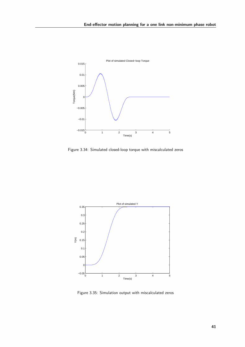
To analyze the effect of the miscalculation of the transfer function zeros, the following transfer function
was introduced in order to obtain the input angle.
y
θ=
1463s4 + 1.258× 10⁻⁹s3 − 6.371× 10⁷s2 + 8.242× 10⁻⁵s+ 1.505× 10¹¹
(s6 + 334.3s5 + 7.198s4 + 1.456× 10⁷s3 + 7.925× 10⁸s2 + 6.396× 10⁹s+ 2.907× 10¹¹)(3.29)
where the new transfer function zeros are:
Zero1,2 = ±202.5884 Zero3,4 = ±50.0614
and the new transfer function poles are:
s1,2 = −15.0428± 213.3005i s3,4 = −0.5513± 19.6926i
s5 = −232.7184 s6 = −70.3933
The location of the zeros and the poles is represented in fig. 3.33:
−250 −200 −150 −100 −50 0 50 100 150 200 250−250
−200
−150
−100
−50
0
50
100
150
200
250
Pole−Zero Map
Real Axis
Imag
inar
y A
xis
Figure 3.33: location of zeros and poles in a closed loop form for miss calculation of transfer function
As before the miscalculation of the transfer function zeros for this case does not pose a significant
problem.
40
End-effector motion planning for a one link non-minimum phase robot
0 1 2 3 4 5−0.015
−0.01
−0.005
0
0.005
0.01
0.015Plot of simulated Closed−loop Torque
Time(s)
Tor
que(
Nm
)
Figure 3.34: Simulated closed-loop torque with miscalculated zeros
0 1 2 3 4 5−0.05
0
0.05
0.1
0.15
0.2
0.25
0.3
0.35Plot of simulated Y
Time(s)
Y(m
)
Figure 3.35: Simulation output with miscalculated zeros
41

3.3 Simulation Results
0 1 2 3 4 5−2
0
2
4
6
8
10
12
14x 10
−3 Plot of simulated Error
Time(s)
Err
or(m
)
Figure 3.36: Simulation tracking error with miscalculated zeros
42

Chapter 4
Path-Following for one link
non-minimum phase robot
The objective of the Path-Following method is to force the non-minimum phase system output to follow
a geometric path without a timing law assigned to it. As presented in chapter 1, systems with unstable
zero dynamics have limited tracking capabilities. The only way to overcome this performance limitation is
to change the input-output structure of the system. This structure can be changed by reformulating the
problem as path-following, rather than reference tracking. With this reformulation, it is possible to add a
new timing law γ(t) that becomes an additional control input. In this chapter we define the path-following
problem, and present two methodologies to solve it. The first one is called Internal model control, and it
has the goal to achieve asymptotic tracking of reference signals; it is demonstrated by Aguiar et al. [2].
The controller that incorporates an internal model of the exosystem is capable to ensure an asymptotic
convergence of the tracking error to zero for every possible reference signal generated by the exosystem.
The second methodology uses the path-following controller to achieve three requirements, a geometric
task, a dynamic task and boundedness of the zero dynamics states.
4.1 Path-Following method with internal model control
The Internal model approach originated in the output regulation problem.
43
4.1 Path-Following method with internal model control
4.1.1 Problem Statement
As previously described, the following linear time-invariant system is assumed:
x(t) = Ax(t) +Bu(t) x(t0) = x0
y(t) = Cx(t) +Du(t)(4.1)
where x(t) is the state, u(t) is the input, and y(t) is the output. The main objective of this method is
to reach and follow a desired geometric path yd(γ). The geometric path yd(γ) can be generated by an
exosystem of the form:d
dγw (γ) = S × w (γ) w (γ0) = w0
yd (γ) = Q× w (γ)(4.2)
where w ∈ R2n is the exogenous state and S + ST = 0. For any timing law γ(t), the path-following error
can be defined as:
e(t) = y(t)− yd(γ(t)) (4.3)
The following problems can be associated to the Path-Following methodology:
Geometric path-following: For the desired path yd(γ), it is necessary to design a controller that achieves:
• Boundedness: the sate x(t) is uniformly bounded for all t > t0, and every initial condition (x(t0), w(γ0)), γ0 =
γ(t0).
• Error convergence: the path- following error e(t) converges to zero as t→∞.
• Forward motion: γ (t) > c for all t > t0, where c is a positive constant.
Speed-assigned path-following: Given a desired speed vd > 0, it is required that γ → vd as t→∞.
As demonstrated by Aguiar et al. [2] and Aguiar [4], we can always assume a small L2-norm of the path
following error,
J =
∞∫0
‖y(t)− yd(t)‖2 dt =
∞∫0
‖e(t)‖2 dt < δ (4.4)
that verifies a δ arbitrarily small in order to consider a perfect tracking problem.
4.1.2 Controller Design - Internal model control
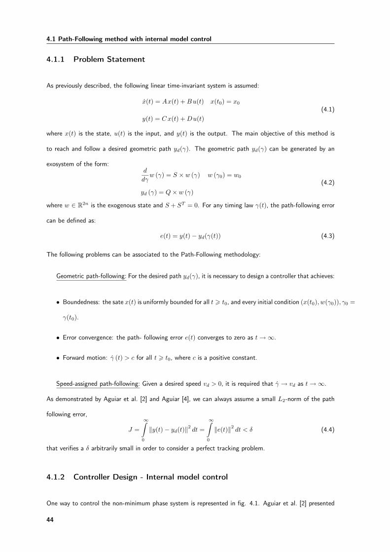
One way to control the non-minimum phase system is represented in fig. 4.1. Aguiar et al. [2] presented
44

Path-Following for one link non-minimum phase robot
System
states
YPath Controler
u
Y2!desired !
"""""""""! controller
Leader
w Velocity
real !
u=K×states+L(v)×w
Figure 4.1: Controller block diagram
one solution to achieve a path controller for (4.1), such that the close loop state is bounded.
If (A,B,C,D) is a non-minimum phase system, the pair (A,B) is stabilizable, the pair (C,A) is
detectable, the number of inputs is as large as the number of outputs (m > q) and the zeros of (A,B,C,D)
do not coincide with the eigenvalues of S (4.2), then for the geometric path-following problem there exist
constant matrices K and L, and a timing law γ(t) such that the feedback law is:
u(t) = Kx(t) + L(γd)w(γ(t)) (4.5)
To calculate the matrices K and L, the following internal model approach is considered :
vdΠS = AΠ +BΓ
0 = CΠ +DΓ−Q(4.6)
As shown before, the Sylvester equations (4.6), are solvable if the system (A,B,C,D) is right-invertible
and its zeros do not coincide with the eigenvalues of vdS. The methodology to solve this equation is
described as follows:
• Transform system (4.6) into the following system:
NewA =
Kron(Ins , A)−Kron(S′, Ina) Kron(Ins , B)
Kron(Ins , C) Kron(Ins , D)
NewB =
0
Q
(4.7)
where ns is the size of the square matrix S and na is the size of the square matrix A.
45
4.1 Path-Following method with internal model control
• From equations (4.7) and (4.6) the following formula is obtained
Π
Γ
= [NewA]−1 [NewB] (4.8)
• Since we now have Π and Γ it is possible to obtain the controller gains K and L. K is calculated
by a minimum quadratic regulator, that minimizes the quadratic cost function,
J (u) =
∞∫0
(xTUx+ uTRu+ 2xTNu
)dt (4.9)
and L is equal to:
L = Γ−K ×Π (4.10)
Now that the path controller design is complete, an evolution rule to γ has to be created, in a way
that:
• limt→∞
γ = γd
• limt→∞
γ = vd
The γ controller has been developed assuming the error function equal to
e = γ − γd (4.11)
Considering a first cost function as
V1 =12e (4.12)
assuming γd = vd (γd), the derivative of equation (4.12) yields:
V1 = e [γ − vd (γd)] (4.13)
Considering now as control law the following equation
γ =dyddγ− k1e (4.14)
with the new error variable Z1
Z1 = γ − dyddγ
+ k1e⇔ γ = Z1 +dyddγ− k1e (4.15)
46

Path-Following for one link non-minimum phase robot
finally the first cost function result is obtained
V1 = e
[Z1 +
dyddγ− k1e−
dyddγ
]⇔ V1 = −k1e
2 + Z1 (4.16)
To ensure that the system evolves to the desired path, another cost function involving the velocity error
must be assumed
V2 = V1 +12Z2
1 (4.17)
obtaining
V2 = −k1e2 + Z1
[e+ γ − d2yd
dγ2d
](4.18)
Using as control law
d2yddγ2d
= γ + e+ k2Z1 (4.19)
finally results
γ =d2yddγ2d
− e− k2
[γ − dyd
dγd
](4.20)
4.1.3 Simulation results
The variable yd was used as a desired path output. Two kinds of paths were computed:
The first path is
yd =(
1− e(−wd×γ) × (1 + wd × γ))yf
dyddγ
=(wde
(−wd×γ) × (1 + wd × γ)− wde(−wd×γ))yf
d2yddγ2
=(−w2
de(−wd×γ) × (1 + wd × γ) + 2w2
de(−wd×γ)
)yf
(4.21)
where the variables wd and yf set the convergence velocity of the system to the final value yf .
Using the same path example as in [18], the second path is
yd = yf sin(γπ
2
); γ ∈ [0, 1]
vs =
ms
π˛dyddγ
˛ arctan(γ−a1a2
)+ ms
2˛dyddγ
˛ γ ∈ [0, 0.5[
ms
π˛dyddγ
˛ arctan(
1−γ−a1a2
)+ ms
2˛dyddγ
˛ γ ∈ [0.5, 1]
vs =
ms
π˛dyddγ
˛ ( a2a22+(γ−a1)
2
)γ ∈ [0, 0.5[
− ms
π˛dyddγ
˛ ( a2a22+(1−γ−a1)
2
)γ ∈ [0.5, 1]
(4.22)
47

4.1 Path-Following method with internal model control
where the parameter a1 sets the width of the low speed regions at the beginning and the end of the path,
while a2 smoothens the square wave, and the ms variable constrains the maximum speed. As expected,
the obtained path in x, y coordinates is the arc represented in fig. 4.2.
−0.1 0 0.1 0.2 0.3 0.4 0.5 0.6−0.1
0
0.1
0.2
0.3
0.4
0.5
0.6Plot of position
position x (m)
posi
tion
y (m
)
Figure 4.2: The path in x, y coordinates
For the results presented in the next section, the following data was used. The system state space
representation in continuous mode is:
A =
0 0 0 0 16040.41 9038.62
0 0 0 0 1143.68 2422.93
0 0 0 0 −81331.5 −57923.19
1 0 0 0 0 0
0 1 0 0 0 0
0 0 1 0 0 0
B =
[607.9 −296.4 −364.7 0 0 0
]TC =
[0 0 0 0.575 1 0
]D = 0
(4.23)
while in this representation, the states are represented in the following way.
q =
θ
η1
η2
θ
η1
η2
(4.24)
48

Path-Following for one link non-minimum phase robot
where the variable θ represents the joint angle. For the controller calculus we used the Matlab LQR
command, which requires the matrix A and B equation (4.23) and the matrix Q and R with the following
values
Q = 100× CT × C
R = 0.001× I(4.25)
which result in the following gain state space matrix
K =[−10.2518 −16.8531 −2.3238 −181.8310 −126.2391 8.1224
](4.26)
The value of the controller L is calculated for different values of speed assignments between 0m/s and
5m/s. The simulation results for the paths in question, refered in equations (4.21) and (4.22) will be
treated in the following section.
First path simulation results
The fist path simulation has the following properties:
• A final y value yf = π/8 in a five seconds simulation
• ωd equal to 20.
In fig. 4.3 we present the desired yd versus the γ variable.
0 0.5 1 1.5 2 2.5 3 3.5 40
0.1
0.2
0.3
0.4
0.5
0.6
0.7
0.8
0.9
1yd vs γ
yd(m
)
γ
Figure 4.3: First Path - Evolution of the desired output versus the path variable
49

4.1 Path-Following method with internal model control
In figs. 4.4 and 4.5 we present the simulation tracking error and the corresponding deformation of the
end-effector. The tracking error and the end-effector deformation converge to zero value, as expected.
0 5 10 15−0.12
−0.1
−0.08
−0.06
−0.04
−0.02
0
0.02Error
Time(s)
Err
or(m
)
Figure 4.4: First Path - Simulation tracking error
0 5 10 15−0.2
−0.15
−0.1
−0.05
0
0.05
0.1
0.15End−effector deformation
Time(s)
End
−ef
fect
or d
efor
mat
ion
(m)
Figure 4.5: First Path - Deformation of the end-effector
Fig. 4.6 presents the evolution of the path variable during the simulation period. In this figure, some
initial variations are visible due to the integrators initial conditions.
50

Path-Following for one link non-minimum phase robot
0 5 10 150
0.05
0.1
0.15
0.2
0.25
0.3
0.35
0.4
0.45
0.5desired γ and real γ
time (s)
γ
Desired γReal γ
Figure 4.6: First Path - Evolution of the desired path variable versus the real path variable
Second path simulation results
The second path shows better results in the end-effector deformation domain, because the path is smoother
and there was no need to introduce initial conditions in the integrators. This was due to the characteristics
of the vs variable which already has initial values, so the path could evolve naturally. Also, the mean
velocity is larger in the first path than in the second path, which could affect the end-effector deformation
results .
By changing the variables of equation (4.22), two paths will be produced. First, a1 = 0.1, a2 = 0.1,
ms = 0.1 and yf = 0.575 × π/2 will be considered. This means that the end-efector will produce a 90
degree rotation. As it is seen in fig. 4.7, the desired velocity profile has non-zero initial and final conditions.
0 5 10 150.02
0.03
0.04
0.05
0.06
0.07
0.08
0.09
0.1
0.11Plot of the simulated velocity
Time(s)
velo
city
(m/s
)
Figure 4.7: Second Path - Simulation velocity profile
51

4.1 Path-Following method with internal model control
So there is no need to introduce integrator’s initial conditions.
In fig. 4.8 the simulation tracking error is presented. It is visible that the maximum error appears at
the maximum speed, and stabilizes to a very small value near zero. One thing that can be highlighted is
the fact that the final value of the error is negative. This means that the system has passed yf by a small
value, and it’s cause can be due to the acceleration profile, since it has non zero initial and final values.
0 5 10 15−1
0
1
2
3
4
5
6
7
8x 10
−3 Error
Time(s)
Err
or (
m)
Figure 4.8: Second Path - Simulation tracking error
Fig. 4.9 presents the evolution of the path variable during the simulation period. Comparing to fig. 4.6
it is observable that this path is smoother, and the control variable has better results. As in fig. 4.8 the
final values of the path variable (fig. 4.9) can be due to the acceleration profile. This kind of property
appeared to be no problem, since this controller is very robust to all kind of signals, as it will be shown in
the validation section.
Analyzing fig. 4.10, it is observed that the end-efector deformation is very small, and this method, with
this path is capable of completely removing it. Other tests were made demonstrating that the deformation
does not depend on how long the path is, opposing the results in chapter 3.
For the second path example, the robustness of the controller was studied for different changes of
the velocity profile. Considering the path in equation (4.22), with a1 = 0.1, a2 = 1, ms = 0.2 and
yf = 0.575× π/2, the end-efector will produce a 90 degree rotation.
With these variables, the velocity profile presented in fig. 4.11 has higher maximum velocity in a
52

Path-Following for one link non-minimum phase robot
0 5 10 150
0.2
0.4
0.6
0.8
1
1.2
1.4Plot of γ Error
Time(s)
γ va
lues
Desired γReal γ
Figure 4.9: Second Path - Evolution of the desired path variable versus the real path variable
0 5 10 15−3
−2.5
−2
−1.5
−1
−0.5
0
0.5
1x 10
−3 End effector deformation
Time(s)
Def
orm
atio
n (m
)
Figure 4.10: Second Path - Deformation of the end-effector
shorter period of time. With a normal controller, a bigger end-effector deformation should be expected.
Nevertheless, this controller defines the system velocity in order to reduce the error and the end-effector
deformations, so, in contrary to what should be expected, the error and end-effector deformations values
didn’t change. Comparing fig. 4.12 with 4.10 and fig. 4.13 with 4.8 we observe the end-effector deformation
remains similar, except for the undershoot at the beginning of the path. As in the previous example
(fig. 4.10), the controller could remove all system deformation. Analyzing the tracking error, all the
characteristics remain (stationary error and values).
53

4.1 Path-Following method with internal model control
0 5 10 150.1
0.105
0.11
0.115
0.12
0.125
0.13
0.135
0.14
0.145Plot of the simulated velocity
Time(s)
velo
city
(m/s
)
Figure 4.11: Second Path - Simulation velocity profile
Figure 4.12: Second Path - Deformation of the end-effector
0 5 10 15−2
0
2
4
6
8
10x 10
−3 Error
Time(s)
Err
or (
m)
Figure 4.13: Second Path - Simulation tracking error
54

Path-Following for one link non-minimum phase robot
Validation
Like before, the effects of external factors, such as external input torque, will be studied.
• Consider the path equation (4.21), with wd = 7 and yf = π/8.
An input torque white noise perturbation with the noise power of 0.1 and sample time of 0.1s has been
introduced. The external perturbation torque is 5 times greater that the normal input torque (fig. 4.14).
These values can be considered as a reasonable external perturbation.
0 5 10 15−4
−2
0
2
4
6
8Plot of the input torque
Time(s)
Tor
que
(N/m
)
Figure 4.14: First Path validation - Simulation input torque (White noise with the noise power of 0.1)
Despite the high input perturbation, the end-effector deformation has reasonable values. Observing
fig. 4.16, after t = 1s, one verifies an increase of end-effector perturbation, due to the velocity decrease,
despite, by observation of fig. 4.15 the end-effector deformation remains unchanged.
In fig. 4.17 it’s visible, in the first 2 seconds, the controller management between the leader position
and the system state boundedness.
55

4.1 Path-Following method with internal model control
Figure 4.15: First Path validation - Deformation of the end-effector (White noise with the noise power of
0.1)
0 5 10 15−0.05
0
0.05
0.1
0.15
0.2
0.25
0.3
0.35
0.4
0.45Output
Time(s)
Y (
m)
Figure 4.16: First Path validation - Simulation output (White noise with the noise power of 0.1)
56

Path-Following for one link non-minimum phase robot
0 5 10 15−0.02
−0.01
0
0.01
0.02
0.03
0.04
0.05Error
Time(s)
Err
or (
m)
Figure 4.17: First Path validation - Simulation tracking error (White noise with the noise power of 0.1)
• Considering the path in equation (4.22), with a1 = 0.1, a2 = 0.1, ms = 0.1 and yf = 0.575× π/2.
A step input torque with the periodicity of 2s and amplitude of 1Nm has been added to the system input.
0 5 10 15−5
0
5
10x 10
−3 Error
Time(s)
Err
or (
m)
Figure 4.18: Second Path validation - Simulation tracking error (External step input torque with amplitude
of 1Nm)
In figs. 4.19 to 4.20, the ability of this controller to eliminate external input torques perturbations can
be observed. The only negative point is the static error. In fig. 4.18 the controller’s difficulties to eliminate
the induced static error are presented.
57
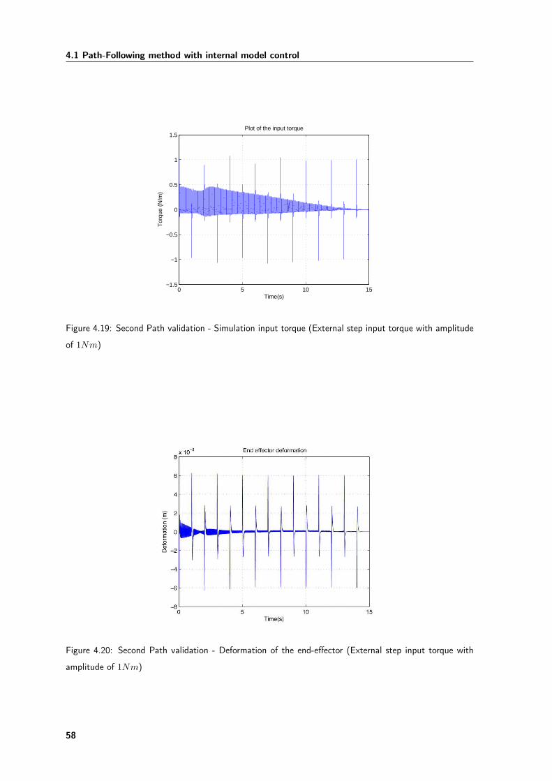
4.1 Path-Following method with internal model control
0 5 10 15−1.5
−1
−0.5
0
0.5
1
1.5Plot of the input torque
Time(s)
Tor
que
(N/m
)
Figure 4.19: Second Path validation - Simulation input torque (External step input torque with amplitude
of 1Nm)
Figure 4.20: Second Path validation - Deformation of the end-effector (External step input torque with
amplitude of 1Nm)
58

Path-Following for one link non-minimum phase robot
Next are presented a series of tests in order to validate the controller in terms of extreme external input
torque, and their implications on the path. The external input torque was changed to white noise with
the noise power of 1 and sample time of 0.1s, and the path properties remain as a1 = 0.1, a2 = 0.1, and
ms = 0.1.
0 5 10 15−0.05
−0.04
−0.03
−0.02
−0.01
0
0.01
0.02
0.03
0.04
0.05Error
Time(s)
Err
or (
m)
Figure 4.21: Second Path validation - Simulation Tracking error (White noise with the noise power of 1)
Since the obtained results were very similar to the results of figs. 4.22 to 4.27, there is only one figure
presented (fig. 4.21). The path properties for figs. 4.22 to 4.27 are a1 = 1, a2 = 0.1 and ms = 1. The
external input torque remains the same.
0 5 10 15−15
−10
−5
0
5
10
15Plot of the input torque
Time(s)
Tor
que
(N/m
)
Figure 4.22: Second Path validation - Simulation input torque (Path properties: a1 = 1, a2 = 0.1 and
ms = 1)
59

4.1 Path-Following method with internal model control
It is also visible that in figs. 4.23, 4.24 and 4.26, the deformation of the end-effector and the path error
values increase, at the same time as the desired theta limitation occurs.
Figure 4.23: Second Path validation - Deformation of the end-effector (Path properties: a1 = 1, a2 = 0.1
and ms = 1)
0 5 10 15−0.06
−0.04
−0.02
0
0.02
0.04
0.06Error
Time(s)
Err
or (
m)
Figure 4.24: Second Path validation - Simulation tracking error (Path properties: a1 = 1, a2 = 0.1 and
ms = 1)
In fig. 4.25, the γ variable signal after t = 6.5s presents a strange behavior. This is caused by limitation
of γ in the interval [0, 1]. Imposing a limitation into the γ, a control value limitation was preset, increasing
the path-variable error. It is also visible that in figs. 4.23, 4.24 and 4.26, the deformation of the end-effector
and the path error values increase, at the same time as the desired path variable limitation occurs.
60
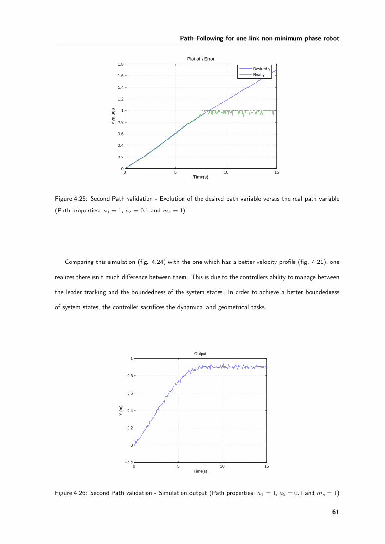
Path-Following for one link non-minimum phase robot
0 5 10 150
0.2
0.4
0.6
0.8
1
1.2
1.4
1.6
1.8Plot of γ Error
Time(s)
γ va
lues
Desired γReal γ
Figure 4.25: Second Path validation - Evolution of the desired path variable versus the real path variable
(Path properties: a1 = 1, a2 = 0.1 and ms = 1)
Comparing this simulation (fig. 4.24) with the one which has a better velocity profile (fig. 4.21), one
realizes there isn’t much difference between them. This is due to the controllers ability to manage between
the leader tracking and the boundedness of the system states. In order to achieve a better boundedness
of system states, the controller sacrifices the dynamical and geometrical tasks.
0 5 10 15−0.2
0
0.2
0.4
0.6
0.8
1Output
Time(s)
Y (
m)
Figure 4.26: Second Path validation - Simulation output (Path properties: a1 = 1, a2 = 0.1 and ms = 1)
61

4.2 Normal Form Path Following
0 5 10 15−20
−10
0
10
20Joint velocity vs Error
Join
t Vel
ocity
(ra
d/s)
Time(s)
0 5 10 15−0.1
−0.05
0
0.05
0.1
Time(s)
erro
r (m
)
Figure 4.27: Second Path validation - Joint velocity versus error (Path properties: a1 = 1, a2 = 0.1 and
ms = 1)
4.2 Normal Form Path Following
Since with the previous controller the end-effector position wasn’t feedback to the controller, a new method-
ology was introduced. Since the goal problem of this thesis is to control a flexible manipulator robot from
point a to point b, and all the bibliography work considers path-following at constant velocity, the adap-
tation from one problem to another is not straightforward. Nevertheless, the Normal Form path following
methodology will be presented here.
Assuming equation (4.1) with uniform relative degree r, and the path yd, the goal is to construct
feedback laws for u and for γ(r), the r(th) derivative of γ, such that the closed-loop solution satisfy the
following requirements.
R1 Geometric task:
lim supt→∞
‖y (t)− yd (γ (t))‖ = 0
R2 Dynamic task:
γ (t) > 0 and limt→∞
γ (t) =∞
R3 Boundedness of the zero dynamics states
System (4.1) is refered as the follower, since it is the one that asymptotically converges to the leader
62
Path-Following for one link non-minimum phase robot
for any admissible leader’s motion. The constraint limt→∞
γ (t) = constant is introduced to disqualify
feedback laws which force the followers output to converge to a point on the path yd. By imposing
γ (t) > 0, the followers output is restricted to the forward motion along the path yd. One of the key
features of this method is the use of the additional feedback law for γ(r).
The starting point for the SISO system controller design is the normal form representation of the
follower (Appendix A).
z = Az +Bzy (4.27)
ζ = Ar,mζ +Br,mu, ζ ,[ζ1 · · · ζn
]T(4.28)
y = Cr,m, y ,[y1 · · · ym
]T(4.29)
where subsystem (4.27) represents the zero dynamics driven by the output y exhibiting the transmission
zeros as the eigenvalues of Az. Subsystem (4.28) represents m chains of r integrators relating the input
u and the output y.
The input variable u is given by:
u =[u ζT zT
] [1 TTu BTz
]T(4.30)
where Tu is an input transformation vector, and Bz is a state transformation vector. The methodology
behind this representation can be found in [19]. There, it is explained the structural decomposition of
MIMO and SISO systems to strictly proper systems (Normal form representation).
The trajectories of system (4.27) - (4.29) are related to the leader’s motion via the error coordinates
ye = y − yd(γ). Furthermore, we define
e =
e1
e2...
em
,
ζ1 − yd1 (γ)
ζ2 − yd2 (γ)...
ζm − ydm (γ)
, ydi (γ) ,
ydi (γ)
ydi (γ)...
y(r)di (γ)
, i = 1, . . . ,m (4.31)
The main distinguishing feature of the path-following problem is that yd (γ) = ∂yd∂γ γ, yd (γ) = ∂2yd
∂γ2 γ2 +
∂yd∂γ γ, . . . give raise to r leader’s states γ . . . γ(r−1), and γ(r) becomes the additional control input w
which controls the leader’s motion in the following system
63

4.2 Normal Form Path Following
z = Azz +Bz (ye + yd (γ)) (4.32)
e = Ar,me+Br,m
(u− y(r)
d (γ)), (4.33)
γ(r) = w (4.34)
Subsystem equation (4.34) is refered as the leader, since it influences the followers zero dynamics equation
(4.32) through the bounded function yd. The ability to stabilize the zero dynamics via a feedback law for
w depends on the geometric properties of the path yd(γ).
The controller approach is to decouple the task R3 of keeping z(t) bounded, from the geometric task
R1. Task R3 is accomplished by designing a feedback law for γ(r) = w, leaving the original control variable
u in (4.33) to be used for R1. Due to boundedness of yd, the feedback law for w can only achieve R3 in
a compact set. The path-following variable will be decomposed into γ(t) = γ(t) + γ(t) where γ(t) = γk,
t ∈ [kT, (k + 1)T ], being T the sampling period. γ(t) is the inter-sample correction to be designed. The
resulting sampled-data equation of the zero dynamics is
zk+1 = AzDzk +BzDvk + dek + dsk (4.35)
To any sampling period T , zk , z(kt), AzD = eAzT , BzD =T∫0
eAzsdsBz, vk , yd (γk) and dek and dsk
are disturbances due to ye(t).
dek =
T∫0
eAz(T−s)Bzye (s+ kT ) ds (4.36)
dsk =
T∫0
eAz(T−s)Bz [yd (γ (s+ kT ))− vk] ds (4.37)
The repeatable path and system (4.35) are essential to construct a stabilizing feedback law γ(r) = w
for the followers zero dynamics equation (4.32), subject to the dynamic task R2. In [5], the methodology
to obtain the controller is explained in more detail. Like the previous controller, the control actuation
64
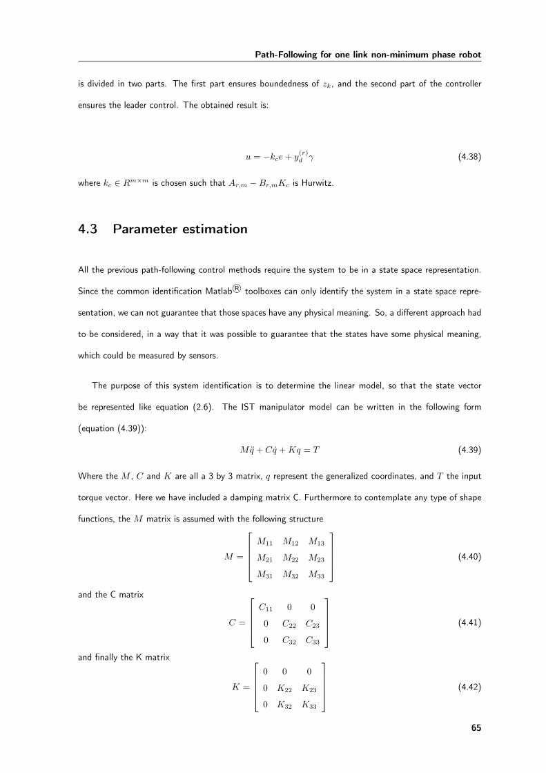
Path-Following for one link non-minimum phase robot
is divided in two parts. The first part ensures boundedness of zk, and the second part of the controller
ensures the leader control. The obtained result is:
u = −kce+ y(r)d γ (4.38)
where kc ∈ Rm×m is chosen such that Ar,m −Br,mKc is Hurwitz.
4.3 Parameter estimation
All the previous path-following control methods require the system to be in a state space representation.
Since the common identification Matlab R© toolboxes can only identify the system in a state space repre-
sentation, we can not guarantee that those spaces have any physical meaning. So, a different approach had
to be considered, in a way that it was possible to guarantee that the states have some physical meaning,
which could be measured by sensors.
The purpose of this system identification is to determine the linear model, so that the state vector
be represented like equation (2.6). The IST manipulator model can be written in the following form
(equation (4.39)):
Mq + Cq +Kq = T (4.39)
Where the M , C and K are all a 3 by 3 matrix, q represent the generalized coordinates, and T the input
torque vector. Here we have included a damping matrix C. Furthermore to contemplate any type of shape
functions, the M matrix is assumed with the following structure
M =
M11 M12 M13
M21 M22 M23
M31 M32 M33
(4.40)
and the C matrix
C =
C11 0 0
0 C22 C23
0 C32 C33
(4.41)
and finally the K matrix
K =
0 0 0
0 K22 K23
0 K32 K33
(4.42)
65
4.3 Parameter estimation
The q vector represents the various generalized coordinates
q = [θ η1 η2]T (4.43)
and the T vector represents the system input
T = [τ 0 0]T (4.44)
Transforming the system equations into state space representation we obtain
q
q
=
03x3 I3x3
−M−1K −M−1C
q
q
+
03x3
M−1
T (4.45)
Just for simplicity we will make the following representation (4.46).
Z =
q
q
; Z =
q
q
A =
03x3 I3x3
−M−1K −M−1C
; B =
03x3
M−1
(4.46)
Now, the system is represented as
Z = AZ +BT ⇔ Z =[A B
] Z
T
(4.47)
which in detail becomes
Z1
Z2
Z3
...
Z6
=[A B
]6×9
Z1
...
Z6
T1
...
T3
(4.48)
For n sample times during trajectory execution, data for q, q , q and τ must be acquired. Renaming
66
Path-Following for one link non-minimum phase robot
M−1ij = Gij , from equation (4.45) and (4.48) the following equation is obtained:
θ
η1
η2
θ
η1
η2
=
0 0 0
0 0 0
0 0 0
0 −K22G12 −K23G13 −K23G12 −K33G13
0 −K22G22 −K23G23 −K23G22 −K33G23
0 −K22G32 −K23G33 −K23G23 −K33G33
1 0 0 0
0 1 0 0
0 0 1 0
−G11C11 −G12C22 −G13C23 −G12C23 −G13C33 −G11
−G12C11 −G22C22 −G23C23 −G22C23 −G23C33 −G12
−G13C11 −G32C22 −G33C23 −G32C23 −G33C33 −G13
θ
η1
η2
θ
η1
η2
τ
(4.49)
Simplifying equation (4.49) yields
θ
η1
η2
θ
η1
η2
=
0 0 0 1 0 0 0
0 0 0 0 1 0 0
0 0 0 0 0 1 0
0 H12 H13 J11 J12 J13 −G11
0 H22 H23 J21 J22 J23 −G12
0 H32 H33 J31 J32 J33 −G13
θ
η1
η2
θ
η1
η2
τ
(4.50)
therefore using a Recursive Least Square (RLS) method (Appendix B), where all the data acquired during
the time of trajectory execution was used, we may obtain the following variables.[H12 H13 J11 J12 J13 −G11
H22 H23 J21 J22 J23 −G12
H32 H33 J31 J32 J33 −G13
] (4.51)
To identify the parameters, a torque input step with amplitude of−2Nm was used. For the data acquisition,
the sampling time used was 0.5ms in order to acquire a sufficient amount of data so that the RLS method
presents better results. The obtained results of identification output values are presented in fig. 4.28.
After using the RLS method, values for the variables in equation (4.51) to a sampling time of 0.0005s were
finally achieved. The system state space matrixes (A,B,C,D) are:
67

4.3 Parameter estimation
0 0.2 0.4 0.6 0.8 1 1.2 1.4−2
−1.5
−1
−0.5
0
0.5
Time (s)
Y (
m)
Identification Output
Figure 4.28: Output values of flexible link identification
AT0=0.0005 =
1 0 0 0.0005 0 0
0 1 0 0 0.0005 0
0 0 1 0 0 0.0005
0 0.3815 −0.0180 0.4923 −0.0013 0.0064
0 −4.8354 −0.2830 0.0352 0.4568 −0.3116
0 −0.3470 0.0284 0.0026 −0.0022 0.4596
(4.52)
BT0=0.0005 =
0
0
0
0.0154
−0.1117
−0.0082
(4.53)
CT0=0.0005 =[
0.575 0.9997 0.0161 0 0 0]
(4.54)
But, since all the control is made at the sample time 0.001s a resampling transformation from sample
time 0.0005s to 0.001s was required.
68

Path-Following for one link non-minimum phase robot
The system representation for T0 = 0.001s is obtained as
A =
1 0 0 0.001 0 0
0 1 0 0 0.001 0
0 0 1 0 0 0.001
0 0.7631 −0.036 0.9846 −0.0027 0.0127
0 −9.6709 −0.5661 0.0704 0.9135 −0.6232
0 −0.6939 0.0568 0.0053 −0.0043 0.9191
(4.55)
B =
0
0
0
0.0307
−0.2233
−0.0163
(4.56)
C =[
0.575 0.9997 0.0161 0 0 0]
(4.57)
D =[
0 0 0 0 0 0]
(4.58)
Comparing the identified system response to an input torque step of −2.3Nm with the real system
response (fig. 4.29), the system main characteristics can be observed, such as non-minimum phase and
gain. The only problem is due to the permanent error, which is to be taken in small consideration, since
the system will not be in free state for a large amount of time.
In fig. 4.30 is presented the quadratic error values, with a average quadratic error of 0.00035862.
69
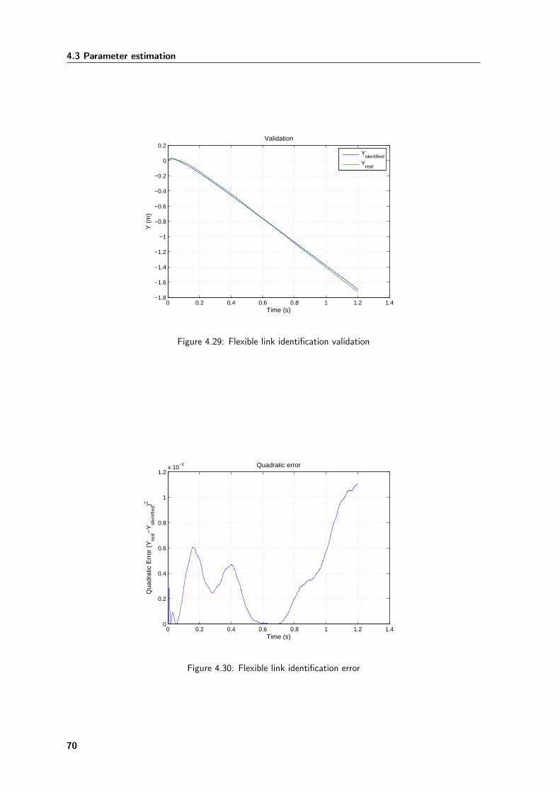
4.3 Parameter estimation
0 0.2 0.4 0.6 0.8 1 1.2 1.4−1.8
−1.6
−1.4
−1.2
−1
−0.8
−0.6
−0.4
−0.2
0
0.2
Time (s)
Y (
m)
Validation
Y
identified
Yreal
Figure 4.29: Flexible link identification validation
0 0.2 0.4 0.6 0.8 1 1.2 1.40
0.2
0.4
0.6
0.8
1
1.2x 10
−3
Time (s)
Qua
drat
ic E
rror
(Y
real
−Y
iden
tifie
d)2
Quadratic error
Figure 4.30: Flexible link identification error
70
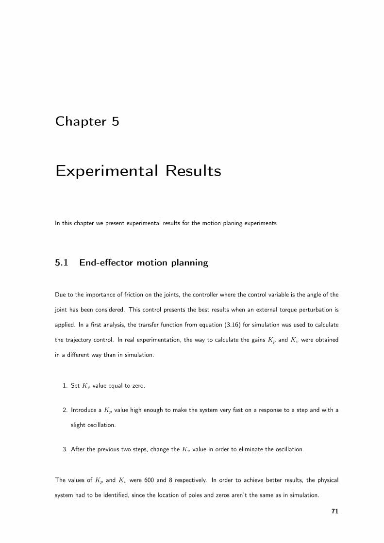
Chapter 5
Experimental Results
In this chapter we present experimental results for the motion planing experiments
5.1 End-effector motion planning
Due to the importance of friction on the joints, the controller where the control variable is the angle of the
joint has been considered. This control presents the best results when an external torque perturbation is
applied. In a first analysis, the transfer function from equation (3.16) for simulation was used to calculate
the trajectory control. In real experimentation, the way to calculate the gains Kp and Kv were obtained
in a different way than in simulation.
1. Set Kv value equal to zero.
2. Introduce a Kp value high enough to make the system very fast on a response to a step and with a
slight oscillation.
3. After the previous two steps, change the Kv value in order to eliminate the oscillation.
The values of Kp and Kv were 600 and 8 respectively. In order to achieve better results, the physical
system had to be identified, since the location of poles and zeros aren’t the same as in simulation.
71

5.1 End-effector motion planning
5.1.1 Identification
The identification of the system was obtained using an input step with amplitude of 0, 02rad and a period
of 64s (figs. 5.1 and 5.2 ).
0 10 20 30 40 50 60 700
0.002
0.004
0.006
0.008
0.01
0.012
0.014
0.016
0.018
0.02
Time (s)
Inpu
t (ra
ds)
Input for identification
Figure 5.1: Identification input
0 10 20 30 40 50 60 70−0.01
−0.005
0
0.005
0.01
0.015
0.02
Time (s)
End
−E
ffect
or d
ispl
acem
ent (
m)
Output for identification
Figure 5.2: Identification output
To identify the system, an ARMAX model with a time sample of 0.001, and a Tustin transformation
from discrete to continuos model was used. This model had the following properties. The system transfer
function considered had a 6 order denominator, a 5 order numerator, considering a noise transfer function
with a 6 order denominator and a 4 order numerator and with one time sample delay.
72
Experimental Results
The transfer function is:
y
θ=
0, 9422s5 − 1481s4 − 4, 955× 106s3 + 7, 761× 109s2 − 9, 703× 1010s+ 9, 118× 1012
(s6 + 1625s5 + 7, 281× 105s4 + 2, 544× 108s3 + 3, 918× 1010s2 + 1, 168× 1011s+ 1, 603× 1013)
(5.1)
Fig. 5.3 presents zeros and poles of the system.
−2500 −2000 −1500 −1000 −500 0 500 1000 1500 2000 2500−400
−300
−200
−100
0
100
200
300
400
Pole−Zero Map
Real Axis
Imag
inar
y A
xis
Figure 5.3: Location of zeros and poles in a close loop form
5.1.2 Control
Now that the system is identified, with recalculation of the trajectory planing and new transfer function,
the system appears to be well behaved since there is almost no vibration on the end-effector (fig. 5.4).
It’s important to notice that if the average velocity of the trajectory becomes too high, the effect of the
non-linearities increases, causing some vibration on the end-effector (fig. 5.5). If the trajectory time is
reduced for the same amplitude, the torque must increase (figs. 5.6 and 5.7).
73

5.1 End-effector motion planning
0 0.5 1 1.5 2 2.5 3 3.5−0.2
0
0.2
0.4
0.6
0.8
1
Time (s)
End
−ef
fect
or d
ispl
acem
ent (
m)
Linear system (Experimental results) t=2,5s yf=0,9032m
Figure 5.4: End-effector vibration at low average velocity
0 0.5 1 1.5 2 2.5 3 3.5−1
−0.8
−0.6
−0.4
−0.2
0
0.2
0.4
Time(s)
End
−ef
fect
or d
ispl
acem
ent (
m)
Non−linear System (Experimental ) results tf=2,5s tf=−0,9032m
Figure 5.5: End-effector vibration at high average velocity
74

Experimental Results
Figure 5.6: Input torque at low average velocity
Figure 5.7: Input torque at high average velocity
75

5.1 End-effector motion planning
76

Chapter 6
Conclusions
In this final chapter, we present the conclusions of the developed work.
6.1 Stable Inversion method
Friction has an important role in the real system. Comparing fig. 3.2 with figs. 5.6 and 5.7 we observe that
the undershoot presented on fig. 3.2 no longer exists. This behavior is due to existing friction on joints,
which acts as a resistive torque. Therefore there is no need to add a negative torque to stop the robot
arm. Another characteristic of this trajectory planning is that it is impossible to eliminate the stationary
error. This characteristic is due to the fact that the controller is a PD controller and by definition it does
not remove any stationary error.
Regarding the control where the input of the system is the angle of the joint, it is evident that this
kind of control is more robust and efficient than the control where the input is the torque. This controller
was the chosen one to the experimental results due to the enormous friction in the joints. There is also
some limitations about the controller since it has been planned around a linear model. When the average
velocity of trajectory becomes too high, the system non-linear effects increase (figs. 5.4 to 5.7).
77

6.2 Path-Following
6.2 Path-Following
Path following is still under intensive study. It is a completely different approach from the standard
control, which involves some advanced mathematics and control theory. One of the major problems on
the implementation of this controller was related with the defined velocity. Since the objective of this
thesis is to control a manipulator robot from point A to point B, and most of path-following solutions
aimed to path-following at constant speed, there were some implementation difficulties. However, we were
able to obtain a path-following controller at continuos state in simulation mode. These results showed
that the path-following controller removes dynamical limitations which reference tracking controllers can’t.
Comparing the external perturbation curves from figs. 3.7 to 3.12 with the curves from figs. 4.14 to 4.27
it’s relevant the ability that the path-following controller has to remove major external disturbances.
Comparing the various studied path types, it is shown that the controller error depends on the path
and it’s limitations. For the first path, there wasn’t any variable limitation so γ can evolve to infinity, but
there is the necessity to insert integrators initial conditions, which develops undesired initial vibrations. For
the second path, γ as been limited between [0, 1], this develops actuation limitations and more difficulty to
attenuate external disturbances. On the other hand, there’s no need to insert integrator initial conditions,
eliminating the initial end-effector vibration.
Since the reference-tracking controller is an open-loop controller, when the reference achieves the final
value, the controller becomes passive, and it doesn’t observe the end-effector deflection, resulting on a
permanent vibration. The path-following ability to separate the dynamic follower controller from the states
boundedness controller, improves the control actuation. Even when the system is reached to the final
value, it still removes the external perturbation. It becomes evident that the path-following controller is a
much more developed and robust controller than the reference tracking controller.
6.3 Future work
One of the reasons to describe the Normal-Form Path-Following controller in this thesis, is due to the fact
that the error from the end-effector position enters directly into the control action. Therefore, it should be
expected better results than currently presented. So, for future work it is highly recommended a profound
78

Conclusions
study and implementation of Normal-form and exo-system path-following controller.
Since in the long run this study aims at the development of a flexible manipulator surgical robot, it
remains to be shown the performance of path-following controllers for robotic medical procedures.
79

6.3 Future work
80

Bibliography
[1] N.G. Hockstein, C.G. Gourin, R. A. Faust, and D.J. Terris. A history of robots: from science fiction
to surgical robotics. Journal of Robotic Surgery, 2007.
[2] A. P. Aguiar, J. P. Hespanha, and P. V. Kokotović. Path-following for nonminimum phase systems
removes performance limitation. IEEE Transactions on Automatic Control, 50(2):234–239, February
2005.
[3] A. P. Aguiar, D. B. Dačic, J. P. Hespanha, and P. Kokotović. Path-following or reference-tracking: An
answer relaxing the limits to performance. In 5th IFAC/EURON Symposium on Intelligent Autonomous
Vehicles, Lisbon, Portugal, July 2004.
[4] A. P. Aguiar. Performance limitations in reference-tracking and path-following. In 44th IEEE Confer-
ence on Decision, Control, and European Control Conference Workshop, editors, New Deveolpments
in Control Performance Limitation Research: A tale in Network Age, Seville, Spain, December 2005.
[5] B. B. Dačic. Path-Following: an Aternative to Reference Tracking. PhD thesis, University of California,
Santa Barbara, June 2005.
[6] M. Benosman and G. Le Vey. Stable inversion of siso nonminimum phase linear systems through
output planning: An experimental application to the one-link flexible manipulator. IEEE Transactions
on Control Systems Technology, 11(4):5–29, July 2003.
[7] M. Benosman and G. Le Vey. End-effector motion planning for one-link flexible robot. Symposium
on Robot Control, pages 561–566, September 2000.
[8] M. Benosman and G. Le Vey. Accurate trajectory tracking of flexible arm end-point. Symposium on
Robot Control, pages 567–572, September 2000.
81
BIBLIOGRAPHY
[9] M. Benosman, F. Boyer, G. Le Vey, and D. Primault. Flexible links manipulators: From modelling to
control. International Journal Of Intelligent And Robotics Systems, 34(4):381–414, 2002.
[10] W. Khalil and E. Dombre. Modeling, Identification and control of robots. Hermes Penton Ltd, 2002.
[11] J. Hauser and R. Hindman. Maneuver regulation from trajectory tracking: feedback linearizable
systems. In Proc. of third IFAC Symp. of Nonlinear Control System Design, 1995.
[12] P. Encarnação and A. Pascoal. 3d path following for autonomous underwater vehicle. 39th IEEE
Conference on Decision and Control, 2000.
[13] H. Kwakernaak and R. Sivan. The maximal achievable accuracy of linear optimal regulators and linear
optimal regulators and linear filters. IEEE Transactions on Automatic Control, 17(1), 1972.
[14] J. M. Martins. Modelling Identification and Control of Flexible Manipulators. PhD thesis, Instituto
Superior Técnico, March 2007.
[15] J. Martins, M. A. Botto, and J. Sá da Costa. Modeling of flexible beams for robotic manipulators.
Multibody System Dynamics, 7:79–100, 2002.
[16] J.M. Martins, Z. Mohamed, M.O. Tokhi, J. Sá da Costa, and M.A. Botto. Approaches for dynamic
modelling of flexible manipulator systems. IEE Proceedings - Control Theory and Applications, 150
(4):401–411, 2003.
[17] J.M. Martins, J. Sá da Costa, and M.A. Botto. Modeling, control and validation of flexible robot
manipulators. In Advances in Computational Multibody Systems, pages 239–268. Springer-Verlag,
2005.
[18] R. Skjetne. The Maneuvering Problem. PhD thesis, Norwegian University of Science and Technology,
Dept. Eng. Cybernetics, Trondheim, Norway, 2005.
[19] B. M. Chen, Z. Lin, and Y. Shamash. Linear Systems Theory - A Structural Decomposition Approach.
Birkhäuser, 2004.
[20] A. N. Paris. Modeling of the dissipative components and force control of rigid-flexible manipulator.
Master’s thesis, Instituto Superior Técnico, 2006.
[21] P. E. Wellstead and M. B. Zarrop. Self-tuning systems. Wiley, 1991.
82

BIBLIOGRAPHY
[22] J.M. Martins, L. Baptista, A. N. Paris, and J. Sá da Costa. Interaction control experiments with a
compliant surface for a rigid-flexible link robot manipulator. In Submitted to 2007 IEEE International
Conference on Robotics and Automation, Roma, Italy, 2006.
[23] M. I. Ribeiro. Análise de Sistemas Lineares, volume 1 and 2. IST Press, Lisbon, 2002.
[24] K. Ogata. Modern Control Engineering, volume Fourth Edition. Prentice Hall, University of Minnesota,
2002.
[25] M. A. Botto. Identificação de Sistemas - Acetatos das Aulas Teoricas. Instituto Superior Técnico,
Lisbon, 2003.
83

BIBLIOGRAPHY
84

Appendix A
Special Coordinate basis
Considering a SISO system characterized by:
Σ : x = Ax+Bu, y = Cx (A.1)
Where x, u and y are the state, the input and the output. Assuming that the transfer function of Σ is not
identically to zero, the following special coordinate basis (SCB) decomposition for Σ is obtained.
Theorem 2. consider the SISO system of A.1. The exist nonsingular state, input and output transfor-
mations Γs ∈ Rn×n, Ti ∈ R and To ∈ R which decompose the state space of Σ into two subspaces xa
and xd these two subspaces correspond to the finite zero and infinite zero structures of Γ, respectively.
The new state space, input and output of the decomposed system are described by the following set of
equations:
x = Γsx, y = Γoy, u = Γiu (A.2)
x =
xa
xd
, xa ∈ Rna , xd ∈ Rnd , xd =
x1
x2
...
xnd
(A.3)
and
xa = Aaaxa + Lady, (A.4)
x1 = x2, y = x1, (A.5)
85

x2 = x3,
...(A.6)
xnd−1 = xnd , (A.7)
xnd = Edaxa + E1x1 + E2x2 + · · ·+ Endxd + u, (A.8)
Where λ(Aaa) contains all the system invariant zeros and nd is the relative degree of Γ.
Figure A.1: Interpretation of structural decomposition of a SISO system
[19] represented a step-by-step algorithm to construct the required Γs, Γi and Γo that realize the
structural decomposition or the special coordinate basis of Σ.
1. Determination of the relative degree The relative degree of Σ can be obtained by differentiating the
output y. Being nd such that:
CB = CAB = · · · = CAnd−2B = 0 (A.9)
and
β = CAnd−1B 6= 0 (A.10)
86
Special Coordinate basis
2. Construction of a preliminary state transformation Let Z0 be an na × n constant matrix, where na
is equal to na = n− nd, such that
Z =
Z0
Zd
=
Z0
C
CA...
CAnd−1
(A.11)
is nonsingular. Z0 can be chosen where whose rows form a basis of the null space of Zd. Being,
x =
x0
x1
x2
...
xnd
= Zx =
Z0
C
CA...
CAnd−1
x (A.12)
thenx1 = Cx = CAx+ CBu = CAx = x2, y = x1,
x2 = CAx = CA2x+ CABu = CA2x = x3,
...
xnd−1 = xnd ,
xnd = Edax0 +nd∑i=1
ξixi + βu
(A.13)
For appropriate Eda, and βi, i = 1, 2, . . . , nd, and
x0 = A00x0 +nd∑i=1
α0,ixi + β0u (A.14)
for some appropriate vectors A00, αo, i = 1, 2, . . . , nd, and β0
3. The elimination of u in the state equation of x0 It follows from A.13 that:
u =1β
[xnd − Edax0 −
nd∑i=1
ξixi
](A.15)
which together with 2 imply that
x0 = A00x0 +nd∑i=1
α0,ixi +β0
β
[xnd − Edax0 −
nd∑i=1
ξixi
](A.16)
x0 = A00x0 +nd∑i=1
α0,ixi +β0
β
[xnd − Edax0 −
nd∑i=1
ξixi
]
x0 = Aaax0 +nd∑i=1
α0,ixi + βxnd
(A.17)
87
4. The elimination of xnd in the state equation of x0 Defining a new state variable,
x0 = x0 − βxnd (A.18)
Obtaining
˙x0 = x0 − βxnd = Aaax0 +nd∑i=1
α0,ixi + βxnd − βxnd
= Aaa(x0 + βxnd
)+
nd∑i=1
α0,ixi
= Aaax0 +nd∑i=1
α0,ixi
(A.19)
for some appropriate constant vectors α0,i, i = 1, 2, . . . , nd, also A.13 can be re-written as:
xnd = Edax0 +nd∑i=1
ξixi + βu (A.20)
for some appropriate ξi, i = 1, 2, . . . , nd.
5. The elimination of x2, . . . , xnd from the state equation of x0 If nd = 1, there’s no further transfor-
mation needed, and can proceed to the following step. Otherwise, let s = 0, x0,0 = x0, α0,0,i = α0,i
and ξ0,i = ξi, i = 1, 2, . . . , nd. It is necessary to carry on the following iterative sub-steps
(a) Eliminate xnd It follows from equation A.19:
˙x0,s = Aaax0,s +nd−s∑i=1
α0,ixi (A.21)
and
xnd = Edax0,s +nd∑i=1
ξs,ixi + βu (A.22)
eliminating xnd−s from the above expression by defining
x0,s+1 = x0,s − (αs,0,nd−s)xnd−s−1 (A.23)
which together with xnd−s−1 = xnd−s imply that
˙x0,s+1 = Aaax0,s+1 +nd−s−1∑i=1
αs+1,0,ixi (A.24)
For some constant vectors αs+1,0,i, i = 1, 2, . . . , nd−s−1. After having eliminated xnd − s in
the above expression, follows
xnd = Edax0,s+1 +nd∑i=1
ξs+1,ixi + βu (A.25)
for some appropriate constant vectors ξs+1,i, i = 1, 2, . . . , nd−s−1.
88

Special Coordinate basis
(b) If s = nd − 2, finish iteration, otherwise set s = s+ 1 and go back to the previous step.
6. Finishing touch Finally, is obtained:
xa = x0,s+1, y = Γoy, u = Γiu =1βu (A.26)
and
Lad = αs+1,0,1, Ei = ξs+1,i, i = 1, 2, . . . , nd (A.27)
where the states are equal to:
xa = Aaaxa + Lady,
x1 = x2, y = x1,
x2 = x3,
...
xnd = Edaxa + E1x1 + · · ·+ Endxnd + u
(A.28)
89

90
Appendix B
Recursive Least Squares equations
The Least Squares method consist in the determination of the parameters vector that minimize the value
of the square error given by [21]
‖v‖2 = ‖F −HX‖2 (B.1)
where v is the vector of the modeling and measurement errors, F is the vector of inputs and H is the
regression matrix. Expanding this expression:
‖v‖2 = (F −HX)T (F −HX)
= (F T −XTHT )(F −HX)
= F TF − F THX −XTHTF +XTHTHX
= F TF − (HX)TF −XTHTF +XTHTHX
= F TF −XTHTF −XTHTF +XTHTHX
= F TF − 2XTHTF +XTHTHX (B.2)
By determining the derivative relative to the parameters vector X and equaling to zero results in
d‖v‖2
dX= HTHX −HTF = 0 (B.3)
So the vector X that minimize the quadratic error is given by
X = (HTH)−1HTF (B.4)
For the Recursive Least Squares method the estimated parameters vector X for an instant t is obtained
by using the last estimation having a parameters vector that converge to the values of the real parameters.
91

For time t− 1 the parameter vector is
X(t− 1) = [HT (t− 1)H(t− 1)]−1HT (t− 1)F (t− 1) (B.5)
At time t, further measurements from the process are acquired enable to form the matrix
H(t) =
H(t− 1)
Y T (t)
, (B.6)
and the vector
F (t) =
F (t− 1)
τ (t)
. (B.7)
The estimation at time t is then given by
X(t) = [HT (t)H(t)]−1HT (t)F (t) (B.8)
From expression (B.6) we get
HT (t)H(t) =[HT (t− 1) Y (t)
] H(t− 1)
Y T (t)
= HT (t− 1)H(t− 1) + Y (t)Y T (t) (B.9)
From equations (B.6) and (B.7) we get the term
HT (t)F (t) =[HT (t− 1) Y (t)
] F (t− 1)
τ (t)
= HT (t− 1)F (t− 1) + Y (t)τ (t) (B.10)
To introduce some shorthand the matrix P (t− 1) and the vector B(t− 1) are defined asP (t− 1) = [HT (t− 1)H(t− 1)]−1
B(t− 1) = HT (t− 1)F (t− 1)
(B.11)
resulting X(t) = P (t)B(t)
X(t− 1) = P (t− 1)B(t− 1)
(B.12)
The terms for the actual time, P (t) and B(t) are given by
P−1(t) = P−1(t− 1) + Y (t)Y T (t) (B.13)
and
B(t) = B(t− 1) + Y (t)τ (t) (B.14)
92
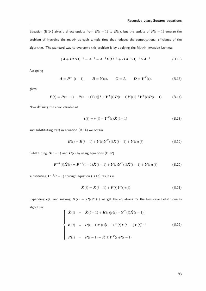
Recursive Least Squares equations
Equation (B.14) gives a direct update from B(t − 1) to B(t), but the update of P (t − 1) emerge the
problem of inverting the matrix at each sample time that reduces the computational efficiency of the
algorithm. The standard way to overcome this problem is by applying the Matrix Inversion Lemma:
(A+BCD)−1 = A−1 −A−1B(C−1 +DA−1B)−1DA−1 (B.15)
Assigning
A = P−1(t− 1), B = Y (t), C = I, D = Y T (t), (B.16)
gives
P (t) = P (t− 1)− P (t− 1)Y (t)[I + Y T (t)P (t− 1)Y (t)]−1Y T (t)P (t− 1) (B.17)
Now defining the error variable as
ε(t) = τ (t)− Y T (t)X(t− 1) (B.18)
and substituting τ (t) in equation (B.14) we obtain
B(t) = B(t− 1) + Y (t)Y T (t)X(t− 1) + Y (t)ε(t) (B.19)
Substituting B(t− 1) and B(t) by using equations (B.12)
P−1(t)X(t) = P−1(t− 1)X(t− 1) + Y (t)Y T (t)X(t− 1) + Y (t)ε(t) (B.20)
substituting P−1(t− 1) through equation (B.13) results in
X(t) = X(t− 1) + P (t)Y (t)ε(t) (B.21)
Expanding ε(t) and making K(t) = P (t)Y (t) we get the equations for the Recursive Least Squares
algorithm:
X(t) = X(t− 1) +K(t)[τ(t)− Y T (t)X(t− 1)]
K(t) = P (t− 1)Y (t)[I + Y T (t)P (t− 1)Y (t)]−1
P (t) = P (t− 1)−K(t)Y T (t)P (t− 1)
(B.22)
93
Related Documents