Trails, lanes, or traffic: Valuing bicycle facilities with an adaptive stated preference survey

This article was originally published in a journal published byElsevier, and the attached copy is provided by Elsevier for the

author’s benefit and for the benefit of the author’s institution, fornon-commercial research and educational use including without

limitation use in instruction at your institution, sending it to specificcolleagues that you know, and providing a copy to your institution’s

administrator.

All other uses, reproduction and distribution, including withoutlimitation commercial reprints, selling or licensing copies or access,

or posting on open internet sites, your personal or institution’swebsite or repository, are prohibited. For exceptions, permission

may be sought for such use through Elsevier’s permissions site at:

http://www.elsevier.com/locate/permissionusematerial

http://www.elsevier.com/locate/permissionusematerial

Autho

r's

pers

onal

co

py

Trails, lanes, or traffic: Valuing bicycle facilitieswith an adaptive stated preference survey

Nebiyou Y. Tilahun a,*, David M. Levinson b,1, Kevin J. Krizek c,2

a Department of Civil Engineering, University of Minnesota, 500 Pillsbury Drive SE, Minneapolis, MN 55455, USAb Department of Civil Engineering, Director, Networks, Economics and Urban Systems (NEXUS) Research Group,

University of Minnesota, 500 Pillsbury Drive SE, Minneapolis, MN 55455, USAc Urban and Regional Planning Program Director, Active Communities Transportation (ACT), Research Group,

University of Minnesota, 301 19th, Ave S., Minneapolis, MN 55455, USA

Received 4 April 2005; received in revised form 28 April 2006; accepted 12 September 2006

Abstract

This study evaluates individual preferences for five different cycling environments by trading off a better facility with ahigher travel time against a less attractive facility at a lower travel time. The tradeoff of travel time to amenities of a par-ticular facility informs our understanding of the value attached to different attributes such as bike-lanes, off-road trails, orside-street parking. The facilities considered here are off-road facilities, in-traffic facilities with bike-lane and no on-streetparking, in-traffic facilities with a bike-lane and on-street parking, in-traffic facilities with no bike-lane and no on-streetparking and in-traffic facilities with no bike-lane but with parking on the side. We find that respondents are willing to travelup to twenty minutes more to switch from an unmarked on-road facility with side parking to an off-road bicycle trail, withsmaller changes associated with less dramatic improvements.� 2006 Elsevier Ltd. All rights reserved.

Keywords: Bicycling; Stated preference; Adaptive stated preference; Bike-lane; Trail

1. Introduction

If bicycling is to be a viable mode of transportation, it must have appropriate facilities. Evaluating what isappropriate requires an understanding of preferences for different types of cycling facilities. In this study weexplore and provide a quantitative evaluation of individual preferences for different cycling facility attributes.This understanding can be incorporated into an evaluation of what facilities are warranted for givenconditions.

0965-8564/$ - see front matter � 2006 Elsevier Ltd. All rights reserved.

doi:10.1016/j.tra.2006.09.007

* Corresponding author. Tel.: +1 612 626 0024; fax: +1 612 626 7750.E-mail addresses: [email protected] (N.Y. Tilahun), [email protected] (D.M. Levinson), [email protected] (K.J. Krizek).

1 Tel.: +1 612 625 6354; fax: +1 612 626 7750.2 Tel.: +612 625 7318; fax: 612 625 3513.

Transportation Research Part A 41 (2007) 287–301

www.elsevier.com/locate/tra

Autho

r's

pers

onal

co

py

The facilities considered here are: (A) Off-road facilities, (B) In-traffic facilities with bike-lane and no on-street parking, (C) In-traffic facilities with a bike-lane and on-street parking, (D) In-traffic facilities with nobike-lane and no on-street parking, and (E) In-traffic facilities with no bike-lane but with on-street parking.The aim is to understand what feature people desire by quantifying how many additional minutes of travelthey would be willing to expend if these features were to be available. This added travel time is the price thatindividuals are willing to pay for the perceived safety and comfort the attributes provide.

A computer based adaptive stated preference survey was developed and administered to collect data for thisstudy. To understand if the value that people attach to attributes of facilities is systematically related to dif-ferent individual and social characteristics, the study has also collected demographic, socioeconomic, house-hold, and current travel mode information from each participant. This information is then used to build anempirical model to evaluate relationships between these independent variables and the additional travel timethat people are willing to expend for different attributes of cycling facilities. In addition to giving a measure ofthe appeal of the attributes under discussion, the model also highlights the social and individual factors thatare important to consider in evaluating what facilities to provide.

Interest in studying bicyclists and cycling environments is growing. Recent papers by a number of authorshave investigated preferences of cyclists and the bicycling environment as well as the relationship between thesupply and use of facilities. Availability of cycling facilities and the type and quality of a cycling facility areimportant determinants of how well they are used. Studies by Dill and Carr (2003), Nelson and Allen (1997)have shown that there is a positive correlation between the number of facilities that are provided and thepercentage of people that use bicycling for commuting purposes. While both studies state that causalitycannot be proved from the data, Nelson and Allen (1997) state that in addition to having bicycle facilities,facilities must connect appropriate origins and destinations to encourage cycling as an alternative commutingmode.

Stated Preference has been used to analyze bicycle route choice in the city of Delft. Their work looked atfacility type, surface quality, traffic levels and travel time in route choice. Bovy and Bradley’s (1985) workfound that travel time was the most important factor in route choice followed by surface type. Another studyby Hopkinson and Wardman (1996) investigated the demand for cycling facilities using stated preference in aroute choice context. They found that individuals were willing to pay a premium to use facilities that aredeemed safer. The authors argue that increasing safety is likely more important than reducing travel timeto encourage bicycling.

Abraham et al. (2004) also investigated cyclist preferences for different attributes using a SP survey in thecontext of route choice. Respondents were given three alternate routes and their attributes and were thenasked to rank the alternatives. The responses were analyzed using a logit choice model. Among other variablesthat were of interest to their study, the authors found that cyclists prefer off-street cycling facilities and low-traffic residential streets. But the authors also claim that this may be due to an incorrect perception of safetyon the part of the respondents, and education about the safety of off-road facilities may change the statedchoice.

Proximity to an off-road bicycle trail plays in route choice decisions. Using intercept surveys along theBurke-Gilman trail in Seattle, Shafizadeh and Niemeier (1997) find that among people who reported originsnear the off-road facility, travel time gradually increases as they are further from trail to a point and thendecreases, leading them to speculate that there may be a 0.5–0.75 mile ‘‘bike shed’’ around an off-road bikepath, within which individuals will be willing to increase their travel time to access that facility and outsideof which a more direct route seems to be preferred.

Aultman-Hall et al. (1997) use GIS to investigate bicycle commuter routes in Guelph, Canada. While com-paring the shortest path to the path actually taken, they found that people diverted very little from the shortestpath and that most bicycle commuters use major road routes. They found little use of off-road trails. Whilethis may be due to the location of the trails and the O–D pair they connect, even in five corridors where com-parably parallel off-road facilities do exist to in-traffic alternatives, they found that commuters used the in-traffic facilities much more often. Only the direct highest quality off-road facility (one that is ‘‘wide with agood quality surface and extends long distance with easy access points’’) seemed to be used relatively more.

Web based stated preference survey’s have been used to estimate a logit model to understand importantattributes for commuter cyclist route choice. Stinson and Bhat (2003) find that respondents preferred bicycling

288 N.Y. Tilahun et al. / Transportation Research Part A 41 (2007) 287–301

Autho

r's

pers

onal

co

py

on residential streets to non residential streets, likely because of the low traffic volumes on residential streets.While their model showed that the most important variable in route preference was travel time, the facility wasalso significant. It was shown that cyclists preferred in-traffic bike-lanes more than off-road facilities. Bothfacility types had a positive effect on utility but the former added more to utility than the latter. In additionthey find that cyclists try to avoid links with on-street parking. Another study by Taylor and Mahmassani(1996) also using a SP survey to investigate bike and ride options, finds that bike-lanes provide greater incen-tives to inexperienced cyclists (defined as those with a ‘‘stated low to moderate comfort levels riding in lighttraffic’’) as compared with more experienced cyclists, with the latter group not showing a significant preferenceto bike-lanes over wide curb lanes.

The results from these papers seem somewhat mixed. Though some of the research has shown a stated pref-erence and revealed preference with some constraints for off-road facilities, others have shown that cyclistsgenerally prefer in-traffic cycling facilities with bike-lanes. Especially in revealed preference cases, the apparentpreference for in-traffic routes may be due to their ability to connect to many destinations in a more directfashion and therefore leading to a lower travel time. In addition route choice may be restricted by facilityavailability, geographic features or missing information. It may also be that for people who regularly bicycle,who are most likely the subjects of the revealed preference studies, travel time and not perceived safety arelikely of utmost importance, as these individuals are more likely to be conditioned to the cycling environment.The actual preference therefore may not be for the in-traffic facility; however, it may be the best alternativeavailable to the cyclists.

Commuter choices are clearly limited by facilities that are available to them. Understanding preferencesand behavior is crucial to providing choices that people desire. This can be best accomplished when the valueof any given improvement in facility attribute is known. Valuation of facility attributes can be done by con-sidering what people are willing to pay for using these facilities. In this study we try to uncover this value bymeasuring how much additional time individuals would be willing to spend bicycling between a given originand destination if alternate facilities with certain attributes were available to them.

In the next section we present the methodology in detail. This is followed by a description of the surveyinstrument and design. The analysis methodology is presented, and then the results.

2. Methodology

The methodology we follow to extract this valuation of attributes uses an adaptive stated preference (ASP)survey. While both revealed and stated preference data can be used to analyze preferences, there are certainadvantages to using the latter method in this case. In using consumer revealed preference, often, a limitationarises because only the final consumer choice is observed. This makes it difficult to ascertain how consumerscame to their final decision. This complication arises because the number of choices that are available to eachconsumer may be very large and information on those alternatives that went into an individual’s decision maynot be fully known. Even in cases where all possible alternatives are known, it is difficult to assess whether thedecision makers considered all available alternatives. In addition, the exact tradeoff of interest may not bereadily available. Even in cases where the tradeoffs seem to be available, one cannot be certain that the con-sumer is acting out his preference for the attributes we are observing. The lack of appropriate data can pose amajor challenge in this respect.

Stated preference surveys overcome these complications because the experimenter controls the choices. InSP settings, the experimenter determines the choices and the respondent considers. While this may not reflectthe actual market choice that individual would make because of the constraints the survey places on the choiceset, it allows us to measure attribute differences between the presented alternatives. Further, by using special-ized forms of SP such as adaptive stated preference (ASP) one can measure the exact value individuals attachto attributes of interest. In this type of survey each option is presented based on choices the respondent hasalready made. This allows for the presentation of choices that the individual can actually consider whileremoving alternatives that the respondent will surely not consider. This methodology has been adopted ina number of contexts, including value of time for commercial vehicle operators (Smalkoski and Levinson,2005), in mode choice experiments (Bergantino and Bolis, 2002), and in evaluating transit improvements(Falzarno et al., 2000) among others.

N.Y. Tilahun et al. / Transportation Research Part A 41 (2007) 287–301 289

Autho

r's

pers

onal

co

py

3. Survey instrument, design and administration

All respondents of the ASP survey were given nine presentations that compared two facilities at a time.Each presentation asks the respondent to choose between two bicycle facilities. The respondent is told thatthe trip is a work commute and the respective travel time they would experience for each facility is given. Eachfacility is presented using a 10 s video clip taken from the bicyclists’ perspective. The clips loop three times andthe respondent is able to replay the clip if they wish.

Each facility is compared with all other facilities that are theoretically of lesser quality. For example, an off-road facility (A) is compared with a bike-lane no on-street parking facility (B), a bike-lane with parking facility(C), a no bike-lane no parking facility (D) and a no bike-lane with parking facility (E). Similarly, the fourother facilities (B, C, D and E) are each compared with those facilities that are theoretically deemed of a lesserquality. The less attractive of the two facilities is assigned a lower travel time and the alternate (higher quality)path is assigned a higher travel time. The respondent goes through four iterations per presentation with traveltime for the more attractive facility being changed according to the previous choice. The first choice set withineach presentation assigns the lesser quality facility a 20 min travel time and the alternate (higher quality) patha 40 min travel time. Travel time for the higher quality facility increases if the respondent chose that facilityand it decreases if the less attractive facility was selected. A bisection algorithm works between 20 and 60 mineither raising or lowering the travel time for the alternate path so that it becomes less attractive if it was chosenor more attractive if the shortest path was chosen. By the fourth iteration, the algorithm converges on the

Fig. 1. Cycling facilities used in the study (A) Off-road bicycle facility. (B) Bike-lane, no parking. (C) Bike-lane, on-street parking.(D) Bike-lane, no parking. (E) No bike-lane, on-street parking.


Autho

r's

pers

onal

co

pymaximum time difference where the respondent will choose the better facility. This way the respondent’s timevalue for a particular bicycling environment can be estimated by identifying the maximum time differencebetween the two route choices that they will still choose the more attractive facility. Pictures of these facilitiesare shown on Fig. 1. Fig. 2 maps the locations of the facilities where the videos were taken in St. Paul,Minnesota.

The procedure used to converge on the time trade-off for the particular facility is illustrated as follows. Ifthe subject first chose the longer option, then the next choice set assigns a higher travel time for the higherquality path (raised from 40 min to 50 min). If the respondent still chooses the longer option, the travel timefor that choice increases to 55 min and the choice is posed again. If on the other hand, the 50 min option is

Fig. 2. Location of facilities used in the adaptive stated preference survey Note: (A) off-road facility; (B) bike-lane, no parking facility;(C) a bike-lane, on-street parking facility; (D) a no bike-lane, no parking facility; (E) a no bike-lane, on-street parking facility.

Table 1Facility pairs compared in the ASP survey

Alternate routes Base route

B Bike-lane, noparking

C Bike-lane with on-streetparking

D No bike-lane, noparking

E No bike-lane withon-street parking

A off-road T1 T2 T3 T4

B Bike-lane, no parking N/A T5 T6 T7

C Bike-lane with on-streetparking

N/A N/A N/A T8

D No bike-lane, no parking N/A N/A N/A T9

Ti represents the average additional travel time user are willing to travel.


Autho

r's

pers

onal

co

pyrejected and the respondent chose the 20 min route, the bisection algorithm will calculate a travel time that isbetween the now rejected option and the previously accepted option, in this case 45 min. By the time therespondent makes a fourth choice, the survey will have either narrowed down the respondents’ preferenceto within two minutes or the respondent has hit the maximum travel time that can be assigned to the longertrip, which is 58.5 min. Table 1 shows the pairs of comparisons that were conducted and used in the analysis.Table 2 shows a sample series of travel time presentations and Fig. 3a and b shows sample screenshots of thesurvey instrument.

The survey was administered in two waves, once during winter and once during summer. The winter andsummer respondents were shown video clips that reflected the season at the time of the survey taken at approx-imately the same location. Our sample for both waves was compromised of employees from the University ofMinnesota, excluding students and faculty. Invitations were sent out to 2500 employees, randomly selectedfrom an employee database, indicating that we would like them to participate in a computer based surveyabout their commute to work and offering $15 for participation. Participants were asked to come to a centraltesting station, where the survey was being administered. A total of 90 people participated in the winter surveyand another 91 people participated in the summer survey, making a total of 181 people. Among these 13 peo-ple had to be removed due to incomplete information leaving 167 people. Of these 167, 68 people indicatedthat they have bicycled to work at least once in the past year. Thirty eight of these sixty eight identified them-selves as regular bicycle commuters at least during the summer. Also, 127 of the 167 people said they havebicycled to somewhere including work in the past year. Further demographic information on the respondentsis given in Table 3.

4. Model specification and results

4.1. Switching point analysis

The adaptive nature of the survey allows us to extract the actual additional minutes each individual is will-ing to travel on an alternate facility. In the context of the survey, this is the maximum travel time beyondwhich the subject would switch to use the lesser quality facility. For each pair of facilities that are comparedduring the summer and the winter, the averages of this switching point are computed and plotted in Fig. 4. Onaverage, individuals are willing to travel more on an alternate facility when the base facility is E (undesignatedwith on-street parking), followed by D (no bike-lane without parking) and C (bike-lane with parking). Forexample individuals are willing to travel further on facility B when the base facility is E, as opposed to Dor C.

Fig. 4 shows the hierarchy between facilities clearly – each of the lines plotted connects the average of themaximum additional travel time that each individual is willing to bicycle over the 20 min that the base facilitywould have provided. For example, looking at the winter data, the top solid line connects the average of themaximum additional time individuals say they would travel on an alternate facility when the base facility is E(in-traffic with parking at 20 min). The alternate facilities are as shown on the horizontal axis. For example,looking at the aggregate data, on average subjects are willing to travel about 23 additional minutes if anoff-road bike-lane was available if the alternative was to bike in traffic with side parking. We can further

Table 2Choice order for a sample presentation

Presentation Facility travel time Choice

Route 1 (min) Route 2 (min)

Choice set 1 40 20 Route 2Choice set 2 30 20 Route 1Choice set 3 35 20 Route 1Choice set 4 37 20 Route 2Ti 36


Autho

r's

pers

onal

co

py

approximate the sampling distribution for the mean additional travel time between each pair of facilities byemploying methods such as the bootstrap.

The bootstrap, which was first developed by Efron in 1979 (Efron and Tibshirani, 1993), approximatesthe sampling distribution of the mean by repeatedly sampling with replacement from the original sampleand calculating the mean of the resamples. The distribution of the means from the re-sampled data is then

Fig. 3. (a) (top) Comparing designated bicycle lanes with no parking with in-traffic bicycling with no parking and (b) (bottom) Samepresentation three iterations later.


Autho

r's

pers

onal

co

pyused to estimate a new mean and to approximate the variability of this estimated mean about the truemean. Here we employ the non-parametric bootstrap, which makes no prior assumptions on the distribu-tion of the statistic. Once the resamples are made, and the means are calculated, one can build a confi-dence interval around the point estimate using the 95 percentiles of the calculated means or using anormal approximation if it is deemed appropriate based on the observed distribution of the bootstrappedmean. The bootstrap analysis is implemented in R using the boot library (R Development Core Team,2004).

Consider the histogram shown in Fig. 5a, it reflects the maximum additional travel time individuals are will-ing to give for facility A (an off-road trail) if their alternative was facility C (an in traffic facility with a bikelane and parking). Employing the non-parametric bootstrap on this data with 5000 resamples, with eachresample having 167 elements, we can see that the bootstrap distribution of the mean is very close to normal(Fig. 5b). The bootstrap distributions of all nine pairs of comparisons lead to symmetric distributions thatshow no evidence of non-normality. The percentile confidence interval based on the actual 2.5% and 97.5%values of the bootstrapped mean, as well as a normal 95% confidence interval are computed for each pairof comparisons. From Table 4, it can be seen that the 95% normal interval and the ordered 95 percentilearound the mean are almost the same.

The bootstrap also allows us to estimate the bias of the sample mean by the difference of the mean from theoriginal sample and the bootstrap mean. For each pair of comparisons, the bias in the mean is also found to bevery small, being consistently less than 3/100th of a minute. The sample mean, the estimate of the bias andthe confidence interval (CI) using the normal distribution and the percentile of the bootstrap are reportedin Table 4 for each pair of comparisons both for the combined and season specific data.

4.2. Model specification

We start with the economic paradigm of a utility maximizing individual, where given a bundle of goods theindividual chooses that bundle which results in the highest possible utility from the choice set. In the current

Table 3Demographic distribution of respondents

Number of subjects 167

Sex% Male 34.5%% Female 65.5%

Age Mean (Standard deviation) 44.19 (10.99)Usual mode (Year round)

% Car 69.7%% Bus 18.5%% Bike 9.2%% Walk 2.6%

Bike commuterAll season 9.2%Summer 22.6%

HH income<$30,000 8.3%$30,000–$45,000 14.3%$45,000–$60,000 19.6%$60,000–$75,000 15.5%$75,000–$100,000 20.2%$100,000–$150,000 17.9%>$150,000 4.2%

HH Size1 25.0%2 32.7%3 16.7%4 20.8%>4 4.8%


Autho

r's

pers

onal

co

py

context then, given two alternatives A and B, the chosen alternative is the one that the subject derives a higherutility from. We can then break down each bundled alternative to its components to understand what amounteach contributes to utility. This will enable us to extract the contribution of each feature of the facility in thechoice consideration of the individual. Mathematically, we would state this as alternative A is selected if UA isgreater than UB, where A and B are the alternatives and U is the utility function.

Maximum Additional Travel Time Between Facility Pairs (Combined Data)

0.00

5.00

10.00

15.00

20.00

25.00

A B C D

Trav

el T

ime B

CDE

Maximum Additional Travel Time Between Facility Pairs (Winter Data)

0.00

5.00

10.00

15.00

20.00

25.00

Trav

el T

ime

A B C D

BCDE

Maximum Additional Travel Time Between Facility Pairs (Summer Data)

0.00

5.00

10.00

15.00

20.00

25.00

30.00

A B C D

Alternate Facility

Trav

el T

ime B

CDE

BaseFacility

BaseFacility

BaseFacility

Alternate Facility

Alternate Facility

Fig. 4. Hierarchy of Facilities. Note: (A) off-road facility; (B) bike-lane, no parking facility; (C) a bike-lane, on-street parking facility;(D) a no bike-lane, no parking facility; (E) a no bike-lane, on-street parking facility.


Autho

r's

pers

onal

co

py

We hypothesize that the utility a user derives from using a bicycle facility depends on the features of thefacility and the expected travel time on the facility. Choices are also affected by individual characteristics that

Freq

uenc

y

14 16 18 20

010

020

030

040

0

time time

Freq

uenc

y

0 10 20 30 40

010

1520

2530

355

Fig. 5. (a) Distribution of the additional travel time for facility C over facility A and (b) The bootstrapped mean for the additional traveltime between facilities A and C (based on 5000 resamples).

Table 4Mean additional travel time between facility pairs and confidence interval of the bootstrapped distribution of the mean

Fac 1 Fac 2 Original mean Bias Standard error Normal 95% CI Percentile 95% CI

Combined data

A B 14.21 0.0223 0.962 (12.30, 16.08) (12.41, 16.17)A C 16.00 0.0136 0.964 (14.10, 17.88) (14.16, 17.92)A D 18.46 �0.0160 0.984 (16.55, 20.41) (16.58, 20.40)A E 23.14 �0.0051 0.939 (21.30, 24.98) (21.26, 24.94)B C 10.13 0.0092 0.973 (8.21, 12.03) (8.25, 12.06)B D 13.73 �0.0008 0.957 (11.85, 15.61) (11.90, 15.62)B E 20.87 0.0245 0.956 (18.97, 22.72) (19.09, 22.84)C E 19.65 �0.0033 0.950 (17.79, 21.51) (17.79, 21.49)D E 18.25 0.0211 1.002 (16.27, 20.20) (16.35, 20.22)

Winter data

A B 15.33 0.0208 1.335 (12.69, 17.92) (12.78, 18.00)A C 13.69 0.0339 1.327 (11.06, 16.26) (11.21, 16.40)A D 17.57 �0.0252 1.344 (14.96, 20.23) (14.99, 20.19)A E 20.66 �0.0025 1.319 (18.08, 23.25) (18.16, 23.28)B C 6.17 �0.0064 1.197 (3.83, 8.52) (3.97, 8.57)B D 10.86 �0.0244 1.180 (8.57, 13.19) (8.58, 13.25)B E 17.45 �0.0101 1.248 (15.02, 19.91 ) (15.02, 19.91)C E 17.39 �0.0097 1.264 (14.92, 19.87) (14.98, 19.92)D E 15.72 0.0074 1.270 (13.22, 18.20) (13.22, 18.22)

Summer data

A B 13.04 �0.0051 1.338 (10.43, 15.67) (10.49, 15.74)A C 18.43 0.0146 1.353 (15.76, 21.07) (15.84, 21.16)A D 19.40 0.0079 1.434 (16.58, 22.20) (16.58, 22.25)A E 25.73 �0.0071 1.292 (23.21, 28.27) (23.18, 28.27)B C 14.28 0.0154 1.397 (11.53, 17.01) (11.63, 17.10)B D 16.75 �0.0128 1.481 (13.86, 19.66) (13.89, 19.68)B E 24.46 �0.0072 1.332 (21.85, 27.07) (21.78, 27.06)C E 22.03 0.0013 1.403 (19.27, 24.77) (19.30, 24.82)D E 20.92 �0.0055 1.485 (18.01, 23.83) (17.96, 23.82)


Autho

r's

pers

onal

co

py

we may not directly observe, but can try to estimate using individual specific variables such as income, sex,age, etc. As discussed earlier, each individual records a response over various alternatives and therefore thedata reflects the repeated choices over the same subject. This implies that the errors are no longer indepen-dently distributed. To overcome this problem, we can specify a generalized linear mixed model (GLMM) thataddresses the ‘within subject’ and ‘between subject’ errors separately (Agresti, 2002). These models take therepeated nature of the responses into consideration, and account for differences between individuals thatreflect taste heterogeneity. In addition to separating the within subject and between subject errors, usingGLMM ensures that the correct error terms are estimated for hypothesis tests. The data analysis for this sec-tion is done using SAS/PROC NLMIXED software (SAS Institute, 2004).

The specification for the mixed logit model is as follows. If we let Yij be the response of individual i onchoice j, and bi be the random term associated with individual i, then for each choice presentation, we canwrite:

ðY ij=biÞ � binomial ð1; pijÞ

logitðpijÞ ¼ U ij þ bi

bi � Nð0; r2Þ

where U is the linear utility derived from each alternative and based on which the choice is made. The utility ofeach alternative is defined in terms of the attributes of the facility. In addition, we are also interested in trendsthat can be explained by individual specific variables. The linear component is then defined as follows:

U ¼ f ðFacility; Travel Time; Season; Individual VariablesÞThe utility of a particular alternative j for individual i can be written as

U ij ¼ V ij þ eij

V ij ¼ b0 þ b1W ij þ b2Oij þ b3Bij þ b4P ij þ b5T ij þ b6Si þ b7Ai þ b8I i þ b9H i þ b10Ci

Where:

W Weather (winter = 1, summer = 0)O Dummy indicating whether the facility is off-road (1 = Yes, 0 = No)B Dummy indicating whether the facility has a bike-lane (1 = Yes, 0 = No)P Dummy indicating whether the facility allows vehicle parking (1 = absent, 0 = present)T Expected travel time on the facility being consideredS Sex (Male = 1, Female = 0)A AgeI Median household income for the reported income range (Inc/1000)H Dummy for household Size (hhsize > 2 = 1, Otherwise = 0)C Cyclist at least during summer (Yes = 1, No = 0)e Gumbel (0, k)

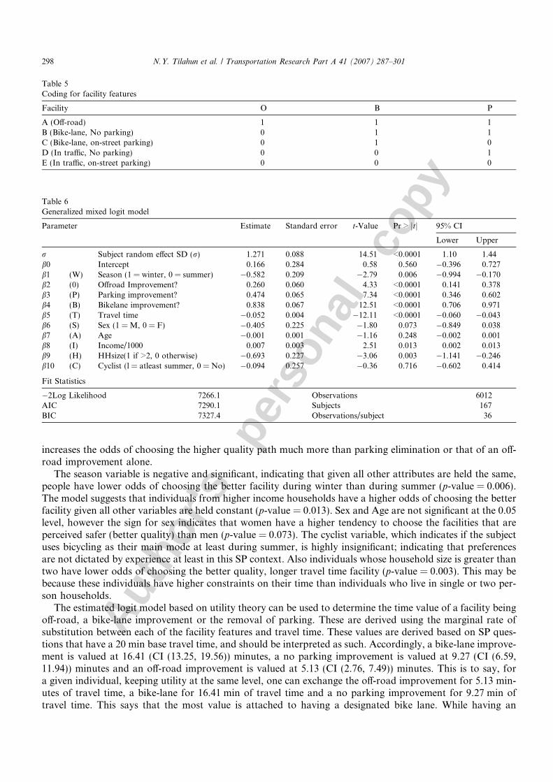
To interpret the model appropriately it is important to note how the dummy variables are coded (Table 5).Variable B represents whether a facility has a designated bike-lane, O represents whether the facility is off-road, and P represents whether a facility has no parking adjacent to it. This would allow separately valuingbike-lanes as well as being off-road. It should be observed that ‘O’ is not equivalent to an off-road trail. ‘B’, ‘O’and ‘P’ together constitute an off-road trail.

The parameter estimates of binomial logit model are given in Table 6. The model is estimated such that thepredicted probabilities reflect the odds of choosing the theoretically better facility. The model suggests thatthere is significant subject-to-subject heterogeneity supporting the use of a mixed model (r = 1.27, CI (1.10,1.44)). The signs of the estimated parameters are as expected. The travel time is negative showing an aversionto longer trips. The improvements (off-road, bike-lane and no parking) all have a positive and significant influ-ence on choice of different magnitudes. Of these three, for a given individual, a bike-lane improvement


Autho

r's

pers

onal

co

pyincreases the odds of choosing the higher quality path much more than parking elimination or that of an off-road improvement alone.

The season variable is negative and significant, indicating that given all other attributes are held the same,people have lower odds of choosing the better facility during winter than during summer (p-value = 0.006).The model suggests that individuals from higher income households have a higher odds of choosing the betterfacility given all other variables are held constant (p-value = 0.013). Sex and Age are not significant at the 0.05level, however the sign for sex indicates that women have a higher tendency to choose the facilities that areperceived safer (better quality) than men (p-value = 0.073). The cyclist variable, which indicates if the subjectuses bicycling as their main mode at least during summer, is highly insignificant; indicating that preferencesare not dictated by experience at least in this SP context. Also individuals whose household size is greater thantwo have lower odds of choosing the better quality, longer travel time facility (p-value = 0.003). This may bebecause these individuals have higher constraints on their time than individuals who live in single or two per-son households.

The estimated logit model based on utility theory can be used to determine the time value of a facility beingoff-road, a bike-lane improvement or the removal of parking. These are derived using the marginal rate ofsubstitution between each of the facility features and travel time. These values are derived based on SP ques-tions that have a 20 min base travel time, and should be interpreted as such. Accordingly, a bike-lane improve-ment is valued at 16.41 (CI (13.25, 19.56)) minutes, a no parking improvement is valued at 9.27 (CI (6.59,11.94)) minutes and an off-road improvement is valued at 5.13 (CI (2.76, 7.49)) minutes. This is to say, fora given individual, keeping utility at the same level, one can exchange the off-road improvement for 5.13 min-utes of travel time, a bike-lane for 16.41 min of travel time and a no parking improvement for 9.27 min oftravel time. This says that the most value is attached to having a designated bike lane. While having an

Table 5Coding for facility features

Facility O B P

A (Off-road) 1 1 1B (Bike-lane, No parking) 0 1 1C (Bike-lane, on-street parking) 0 1 0D (In traffic, No parking) 0 0 1E (In traffic, on-street parking) 0 0 0

Table 6Generalized mixed logit model

Parameter Estimate Standard error t-Value Pr > jtj 95% CI

Lower Upper

r Subject random effect SD (r) 1.271 0.088 14.51 <0.0001 1.10 1.44b0 Intercept 0.166 0.284 0.58 0.560 �0.396 0.727b1 (W) Season (1 = winter, 0 = summer) �0.582 0.209 �2.79 0.006 �0.994 �0.170b2 (0) Offroad Improvement? 0.260 0.060 4.33 <0.0001 0.141 0.378b3 (P) Parking improvement? 0.474 0.065 7.34 <0.0001 0.346 0.602b4 (B) Bikelane improvement? 0.838 0.067 12.51 <0.0001 0.706 0.971b5 (T) Travel time �0.052 0.004 �12.11 <0.0001 �0.060 �0.043b6 (S) Sex (1 = M, 0 = F) �0.405 0.225 �1.80 0.073 �0.849 0.038b7 (A) Age �0.001 0.001 �1.16 0.248 �0.002 0.001b8 (I) Income/1000 0.007 0.003 2.51 0.013 0.002 0.013b9 (H) HHsize(1 if >2, 0 otherwise) �0.693 0.227 �3.06 0.003 �1.141 �0.246b10 (C) Cyclist (l = atleast summer, 0 = No) �0.094 0.257 �0.36 0.716 �0.602 0.414

Fit Statistics

�2Log Likelihood 7266.1 Observations 6012AIC 7290.1 Subjects 167BIC 7327.4 Observations/subject 36


Autho

r's

pers

onal

co

pyoff-road facility would certainly increase the utility of the individual, most of the gains of an off-road facilityseem to be derived from the fact that such facilities provide a designated bike lane. The absence of parking isalso valued more than taking the facility off-road Table 7.

4.3. Switching point analysis

An alternate specification of the model looks at time as a dependent variable, and features of the facility asindependent variables along with demographic covariates. The dependent variable is the maximum additionalminutes individuals would be willing to travel for attributes of an alternate facility. This is the switching pointbeyond which individuals would take the lesser quality facility. This specification employs a linear mixed mod-els approach to account for the repeated measurements taken over the same subject as was done in the bino-mial logit case. This approach yields similar patterns in the order of valuation of the different attributes of thefacilities and the expected directions of the parameter estimates. The results of this model are reported in Table8.

4.4. Comparison

A side by side comparison of the logit and linear models is not possible; however, we can compare the val-ues derived for different facility pairs based on the logit model and the linear model for a given individual. Thisis given in Table 9 and Fig. 6. As can be seen from Table 9, most comparisons have confidence intervals thatoverlap, however the estimates from the logit model are more narrowly estimated as compared to the linearmodel. In addition, the logit model confidence intervals as well as point estimates closely approximate what isobserved in the row data. For instance, between facilities A and D, the logit model estimates a 21.5 min (CI(17.1, 25.9)) value while the mean from the raw data is 19.4 min (CI (16.6, 22.2)).

Table 7Time values of facility attributes

Attribute Calculated Estimate Standard error t-Value Pr > jtj 95% CI

Lower Upper

O Offstreet �b2/b5 5.13 1.20 4.27 <0.0001 2.76 7.49P Parking improvement �b3/b5 9.27 1.36 6.83 <0.0001 6.59 11.94B Bikelane improvement �b4/b5 16.41 1.60 10.27 <0.0001 13.25 19.56

Table 8Linear model

Parameter Estimate Standard error t-Value Pr > jtj 95% CI

Lower Upper

r Subject random effect SD (r) 8.913 0.512 17.39 0.000 7.91 10.05b0 Intercept 5.794 3.285 1.76 0.078 �0.651 12.239b1 (W) Season (1 = winter, 0 = summer) �3.833 1.460 �2.63 0.010 �6.716 �0.950b2 (0) Offroad improvement? 2.284 0.421 5.43 0.000 1.459 3.109b3 (P) Parking improvement? 3.520 0.447 7.88 0.000 2.644 4.397b4 (B) Bikelane improvement? 5.820 0.447 13.03 0.000 4.943 6.696b5 (S) Sex (1 = M, 0 = F) �3.327 1.574 �2.11 0.036 �6.435 �0.218b6 (A) Age 0.161 0.070 2.32 0.022 0.024 0.299b7 (I) Income/1000 0.032 0.021 1.51 0.133 �0.010 0.073b8 (H) HHsize (1 if >2, 0 otherwise) �3.748 1.606 �2.33 0.021 �6.920 �0.577b9 (C) Cyclist (1 = atleast summer, 0 = No) �2.038 1.798 �1.13 0.259 �5.590 1.513

Fit statistics

�2Log Likelihood 10838.824 Observations 1503AIC 10862.82 Subjects 167BIC 10926.45 Observations/subject 9


Autho

r's

pers

onal

co

pyThe overall assessment of the models suggests that designated bike lanes seem to be what are most desired.

It is also important to consider that both the linear and logit models found no evidence against the hypothesisthat preferences between cyclists and non-cyclists are the same. This is encouraging in many respects, becauseit avoids the dilemma of which interest to serve. The policy implication is that by addressing this commonpreference, we can ensure cyclists receive the facilities they prefer and non-cyclists get the facilities that theycould at least consider as a viable alternative.

5. Conclusion

This paper analyzes preferences for different cycling facilities using a computer-based adaptive stated pref-erence survey with first person videos. Using the survey on 167 randomly recruited individuals, we derive thevalues that users attach to different cycling facility features and expose which are most important. The choicedata was collected based on individual preferences between different facilities having different travel times, butthe same origin and destination. From the raw data we have demonstrated that a hierarchy exists between thefacilities considered and we have extracted a measure of how many additional minutes an individual is willingto expend on an alternate facility if it were available and provided certain features that were not available onthe base facility. The data was then used to fit a random parameter logit model using a utility maximizingframework. A linear model was also estimated and compared to the results from the mixed logit model.

Table 9Comparison of travel time values between facilities using the linear model and the logit model

Facilitiescompared

Logitmodel

Logit modelCI

Linearmodel

Linear model CI Mean (aggregate rawdata)

Bootstrap 95%Normal CI

A vs B 5.1 (2.8, 7.5) 8.1 (1.7, 14.6) 13.0 (10.4, 15.7)A vs C 14.4 (10.5, 18.3) 11.6 (5.2, 18.1) 18.4 (15.8, 21.1)A vs D 21.5 (17.1, 25.9) 13.9 (7.5, 20.4) 19.4 (16.6, 22.2)A vs E 30.8 (24.7, 36.9) 17.4 (11.0, 23.9) 25.7 (23.2, 28.3)B vs C 9.3 (6.6, 11.9) 9.3 (2.9, 15.8) 14.3 (11.5, 17.0)B vs D 16.4 (13.3, 19.6) 11.6 (5.2, 18.1) 16.7 (13.9, 19.7)B vs E 25.7 (20.6, 30.7) 15.1 (8.7, 21.6) 24.5 (21.9, 27.1)C vs E 16.4 (13.3, 19.6) 11.6 (5.2, 18.1) 22.0 (19.3, 24.8)D vs E 9.3 (6.6, 11.9) 9.3 (2.9, 15.8) 20.9 (18.0, 23.8)

Time Value of Facilities using Alternate Models

0

5

10

15

20

25

30

35

A vs

B

A vs

C

A vs

D

A vs

E

B vs

C

B vs

D

B vs

E

C v

s E

D v

s E

Compared Facilities

Estim

ated

Tim

e Va

lue

betw

een

Faci

litie

s

logit model

linear model

raw data

Fig. 6. Comparison of the estimates of the additional time willing to travel between facility pairs based on logit model, linear model andthe raw data.


Autho

r's

pers

onal

co

py

The results show that users are willing to pay the highest price for designated bike-lanes, followed by theabsence of parking on the street and by taking a bike-lane facility off-road. In addition, we are able to extractcertain individual characteristics that are indicative of preferences such as age, household structure and looseconnections with sex and household income. Such an understanding can be incorporated into the planningprocess to help planners make appropriate recommendations and investment decisions in developing bicyclefacilities that are more appealing to the public.

References

Abraham, J., McMillan, S., Brownlee, A., Hunt, J.D., 2004. Investigation of cycling sensitivities. Presented at 81st Annual Meeting of theTransportation Research Board, Washington, DC.

Agresti, A., 2002. Categorical Data Analysis, second ed. John Wiley & Sons, Inc., Hoboken, New Jersey.Aultman-Hall, L., Hall, F., Baetz, B., 1997. Analysis of bicycle commuter routes using geographic information systems: Implications for

bicycle planning. Transportation Research Record: Journal of the Transportation Research Board, No, 1578, TRB, National ResearchCouncil, Washington, DC., pp. 102–110.

Bergantino, A., Bolis, S., 2002. An adaptive conjoint analysis of freight service alternatives: Evaluating the maritime option. In: IAME2002 Conference Proceedings, Panama.

Bovy, P., Bradley, P., 1985. Route choice analyzed with stated preference approaches. Transportation Research Record 1037, TRB,National Research Council, Washington, DC.

Dill, J., Carr, T., 2003. Bicycle commuting and facilities in major U.S. cities: If you build them, commuters will use them – another look.CD-ROM. Transportation Research Board, National Research Council, Washington, DC.

Efron, B., Tibshirani, R., 1993. An Introduction to the Bootstrap. Chapman and Hall, New York.Falzarno, S., Hazlett, R., Adler, T., 2000. Quantifying the value of transit station and access improvements for Chicago’s rapid transit

system. Presented at 80th Annual Meeting of the Transportation Research Board, Washington, DC.Hopkinson, P., Wardman, M., 1996. Evaluating the demand for new cycle facilities. Transport Policy 2 (4), 241–249.Nelson, A.C., Allen, D., 1997. If you build them, commuters will use them. Transportation Research Record: Journal of the

Transportation Research Board, No, 1578, TRB, National Research Council, Washington, DC., pp. 79–83.R Development Core Team 2004. R: A language and environment for statistical computing. R Foundation for Statistical Computing,

Vienna, Austria. ISBN 3-900051-07-0, URL <http://www.R-project.org>.SAS/NLMIXED software, Version 9 of the SAS System for Windows. Copyright � 2004 SAS Institute Inc., Cary, NC, USA.Shafizadeh, K., Niemeier, D., 1997. Bicycle journey-to-work: travel behavior characteristics and spatial attributes. Transportation

Research Record: Journal of the Transportation Research Board, No. 1578, TRB, National Research Council, Washington, DC.,pp. 84–90.

Smalkoski, B., Levinson, D., 2005. Value of time for commercial vehicle operators. JTRF 44 (1).Stinson, A.S., Bhat, C.R., 2003. An Analysis of Commuter Bicyclist Route Choice Using a Stated Preference Survey. CD-ROM.

Transportation Research Board. National Research Council, Washington, DC.Taylor, D., Mahmassani, H. 1996. Analysis of stated preference for intermodal bicycle-transit interfaces. In: Transportation Research

Record: Journal of the Transportation Research Board, No. 1556, TRB, National Research Council, Washington, DC., pp. 86–95.


Trails, lanes, or traffic: Valuing bicycle facilities with an adaptive stated preference survey

Documents