Trade, Technology, and Agricultural Productivity

Trade, Technology, and AgriculturalProductivity

Farid Farrokhi

Purdue University

Heitor S. Pellegrina

NYU Abu Dhabi∗

June 2021

Abstract

We examine the contribution of trade to the rise of modern agriculture, taking into

account interactions between trade, input requirements, and technology adoption. We

develop and estimate a new multi-country general equilibrium model that incorporates

producers’ choices of which crops to produce and with which technologies, at the level

of grid-cells covering the Earth’s surface. We find that trade cost reductions in agricul-

tural inputs and the international transmission of productivity growth in the agricul-

tural input sector since the 1980s induced large shifts from traditional, labor-intensive

technologies to modern, input-intensive ones, with important global and distributional

implications for productivity and welfare.

Keywords: Trade, Technology, Intermediate Inputs, Productivity, Agriculture

∗We are grateful to Kerem Cosar, Jonathan Eaton, Tom Hertel, Russell Hillbery, David Hummels, JeanImbs, Andrei Levchenko, Volodymyr Lugovskyy, Samreen Malik, Lucas Scottini, Sebastian Sotelo, FarzadTaheripour, Chong Xiang, and participants in seminars at Purdue, NYU Abu Dhabi, NOITS, NBER Agri-cultural Markets and Trade Policy, NEUDC, NBER Agricultural Risk, UEA European Meeting, and ETOS-FREIT for helpful discussions and feedback. We thank Karolina Wilckzynska and Yuliya Borodina forexcellent research assistance. We would like to thank the help from the ITaP team of Purdue with our high-performance computing. This paper has previously circulated as “Global Trade and Margins of Productivityin Agriculture”. Email: [email protected] and [email protected].

1

1 Introduction

Production technologies that have enhanced the conditions of human life around the world

often require the use of certain intermediate inputs, ranging from semiconductors for elec-

tronics, garment machinery for textiles, or tractors for agriculture. In many countries and

industries, producers largely depend on international trade to procure these inputs. The in-

teraction between technology choices, input requirements, and international trade is, there-

fore, important for examining the welfare implications of technology adoption across the

world.

One sector in which technology adoption has had a dramatic effect on economic welfare is

agriculture. Agricultural modernization, reflected by a shift from traditional, labor-intensive

technologies to modern, input-intensive ones, has long been argued to be a central feature of

economic development (Johnston and Mellor, 1961; Schultz et al., 1968; Gollin, Parente, and

Rogerson, 2007). The role of international trade for such a shift, however, has not yet been

explored. The importance of addressing this gap is reinforced the moment we confront data:

across countries, on average two-thirds of every dollar spent on agricultural inputs such as

machinery and fertilizers that are required for the use of modern agricultural technologies

are paid to foreign suppliers. This paper provides the first study of the effects of trade on

the rise of modern agriculture and the implications for welfare and agricultural productivity

around the world.

Methodologically, agriculture gives us a rare opportunity of observing direct measures

of factor productivities—measures that are otherwise inferred from residuals of production

functions. The mapping between conditions of land and climate to crop output is scientifi-

cally well-measured, and that mapping is known under which technology, whether traditional

or modern, is adopted. We bring in measures of land productivity from the Food and Agri-

culture Organization’s Global Agro-Ecological Zones (FAO-GAEZ) for every crop-technology

pair at more than a million grid cells (fields) around the world. We exploit these extremely

rich data in a new quantifiable, general-equilibrium model that incorporates micro-level

choices of which crops to grow and with which technology to grow them.

We tune our general equilibrium analysis to address two broad questions. First, what

were the consequences of the fall of trade barriers in the recent decades, often referred to

as “globalization”, on technology adoption, agricultural productivity, and welfare around the

world? We are particularly interested in comparing the relative importance of globalization

in agricultural inputs (via technology adoption) to globalization in agricultural outputs (via

international crop specialization). Second, how was productivity growth in the production

of agricultural inputs, such as farm machinery, fertilizers, and pesticides, transmitted across

2

borders by means of trade? Of our particular interest is the relative importance of the

productivity growth coming from foreign sources of inputs compared to domestic ones. In

answering these questions, we also seek to understand the distributional implications of trade

across countries with different levels of development.

In our framework, we consider a world that consists of multiple countries, each encom-

passing numerous fields. In every field, crops can be produced by different technologies

that are characterized by their intensities of land, labor, and agricultural inputs. Choices

of crops and technologies depend on both market and agro-ecological conditions. As for

market conditions, higher relative prices of a crop encourage the allocation of resources to

the production of that crop, and higher wages or lower prices of inputs incentivize the use

of labor-saving, input-intensive technologies. As for agro-ecological conditions, we adopt a

parsimonious, yet flexible specification that allows us to exploit the field-level measures of

land productivity from FAO-GAEZ. Specifically, we let land productivities be heterogeneous

within every field based on a generalized Frechet distribution, which gives rise to tractable

field-level production possibility frontiers (PPFs). These PPFs are fully characterized by

two parameters that discipline the marginal rates of substitution between crops and between

technologies within crops (i.e., the curvature of the PPF), and agro-ecological parameters

that shift the scale of production in a field for every crop-technology pair (i.e., the scale of

the PPF).

Our framework generalizes previous models of agricultural trade and land-use, including

Costinot, Donaldson, and Smith (2016) and Sotelo (2020), by incorporating choices of tech-

nologies in addition to crops. In doing so, we introduce a new source of gains from trade.

It is well-studied that trade in crops (i.e. agricultural outputs) generates efficiency gains by

making room for international crop specialization. In our framework, trade in agricultural

inputs can also generate efficiency gains by incentivizing the use of modern, input-intensive

technologies. We trace the marks of this mechanism on the welfare gains from trade. Using

a pared down version of our model, we show that, relative to the well-known result of Arko-

lakis, Costinot, and Rodriguez-Clare (2012), a novel term appears in the gains from trade

formula that depends on the share of land under traditional technology and a parameter

that governs the marginal rate of substitution between traditional and modern technologies

(i.e., the curvature of the PPF along the technology dimension).

To take our model to data, we collect and organize country and field level data from sev-

eral different sources. Our final data cover 65 countries and a rest-of-the-world region in year

2007, with information on trade, production, and agricultural input use—including farm ma-

chinery, fertilizers, and pesticides. To estimate demand side parameters, we follow standard

practices. To estimate model-implied PPFs, we search for the values of the two parame-

3

ters controlling the curvature of PPFs by minimizing the distance between moments in the

data and their model counterparts, while using the FAO-GAEZ data to calibrate field-level

shifters. Specifically, one set of our moments is based on spatial variations in the land use of

crops: Countries with relatively larger agro-ecological productivity in a crop tend to produce

that crop more intensively if PPFs feature less curvature in substitution between crops. An-

other set of our moments is based on cross-country measures of agricultural input-intensity:

Countries with higher wages and lower input prices tend to adopt modern technologies more

intensively if PPFs feature less curvature in substitution between technologies.

Our estimated model fits several key cuts of data very well. It closely fits the data on

output quantities, prices, and land use of crops across countries. It also predicts very well

the relationship between countries’ level of economic development and several key measures

of agricultural input-intensity.

Based on spatial variations in market and agro-ecological conditions, our model implies

large cross-country differences in technology choices: the share of land under modern agri-

cultural technology is 35% in the first quartile of the GDP per capita and 95% in the fourth

quartile. Before turning to our counterfactual exercises, we utilize our estimated model to

carry out a decomposition exercise that sheds light on the sources of agricultural technology

differences across the world. Our decomposition exercise shows that variations in prices and

wages (market conditions) account for two-thirds of model-implied differences in technology

choice, and that variations in agro-ecological propensity (natural conditions) account for the

remaining one-third. Zooming into the market conditions, the contribution of agricultural

input prices are as important as wages, and cross-country differences in access to foreign

inputs account for about one-third of variations in input prices.

We then perform counterfactual exercises to provide quantitative answers to our two

broad questions. We start by examining how reductions in trade costs in the recent decades

shaped agricultural productivity and welfare across the world. To do so, we simulate a

counterfactual in which trade costs in agricultural outputs and inputs are set back to their

estimated level in 1980, and compare the resulting equilibrium with that in the baseline of

2007. We find notable productivity gains, reflected by 4.0% increase in food consumption

and 2.5% rise in welfare at the global scale.

To separate the effects of input-side mechanisms (by way of technology adoption) from

output-side mechanisms (by way of international crop specialization), we run two additional

counterfactuals in which we examine, separately, globalization in only agricultural inputs

and only agricultural outputs. Comparing their implications for agricultural productivity,

food consumption, and welfare at the global scale, we find that mechanisms on the input

side are quantitatively as important as those on the output side. These results tell us that

4

we would miss much in evaluating productivity and welfare effects of globalization if we were

to ignore input-side mechanisms.

In addition, we find that the distributional implications of these two mechanisms are

substantially different. Globalization in agricultural outputs particularly benefits low-income

countries because they have a larger expenditure share on food. This leads to lower welfare

inequality between low- and high-income countries. In contrast, due to two distinct channels,

globalization in agricultural inputs benefits middle-income countries the most. First, it

increases the adoption of modern technologies; second, it increases productivity in the land

already using modern technology. While the first channel is virtually muted in high-income

countries (since they already have a large share of land under modern technologies), the

second channel is negligible in low-income countries (since they have a small share of land

under modern technologies). As such, globalization in agricultural inputs widens the gap

between low- and middle-income countries, while compressing the gap between middle- and

high-income countries.

Lastly, we turn to examining our second research question, in which we study how trade

transmits the benefits of productivity growth in the production of agricultural inputs across

national borders. To this end, we first simulate a counterfactual in which we set produc-

tivities in the agricultural input sector for all countries to their estimates in 1980, as well

as 66 counterfactuals in which we change these productivities country by country, one at a

time. We next compare, for each country, the counterfactual outcomes from input produc-

tivity growth in only that country versus productivity growth in all countries. We take the

difference between welfare gains in these two counterfactual scenarios as the contribution of

the foreign productivity shocks that are transmitted by way of trade in agricultural inputs.

We find this contribution to be around 40% for an average country, which indicates that

international trade played a major role in sharing the benefits of productivity growth in the

agricultural input sector across national borders in recent decades.

These benefits, however, were substantially lower for low-income countries. Interna-

tional productivity growth in the agricultural input sector brings about lower prices of

internationally-supplied agricultural inputs. These lower prices particularly benefit agri-

cultural productivities in middle- and high-income countries that have a more widespread

use of modern technologies. Consequently, low-income countries lose their competitiveness

in exports of agricultural products, which explains their smaller gains from lower prices of

agricultural inputs in international markets.

Related Literature. We introduce technology choices to general equilibrium models of

agricultural trade and specialization—e.g., Costinot, Donaldson, and Smith (2016)—that

5

can be taken to rich spatial data.1This is an important contribution for three reasons. First,

conceptually, long-run changes to trade barriers, climate conditions, or environmental reg-

ulations likely affect not only which crops farmers grow in a region but also with which

methods they produce them. Second, by developing a framework that allows for multiple

technology choices, we provide a method that can fully exploit the richness of the data from

FAO-GAEZ.2 Third, our formulation, based on a generalized Frechet distribution, presents

a parsimonious way of incorporating flexible choices of both crops and technologies, bringing

new mechanisms through which trade shapes productivity.3

This paper also speaks to the literature on the welfare implications of international trade,

highlighting the role of multinational production (Ramondo and Rodrıguez-Clare, 2013), firm

heterogeneity (Eaton, Kortum, and Kramarz, 2011), and input-output linkages (Caliendo and

Parro, 2015)— among other mechanisms (for a review, see Costinot and Rodrıguez-Clare

(2014)). In addition, our work relates to studies that evaluate different channels through

which trade in inputs increases productivity, including variety gains (Goldberg, Khandelwal,

Pavcnik, and Topalova, 2010), quality upgrading (Fieler, Eslava, and Xu, 2018), and global

sourcing (Antras, Fort, and Tintelnot, 2017; Blaum, Lelarge, and Peters, 2018; Farrokhi,

2020).4 We contribute to these strands of trade literature by embedding into a multi-country

1A few recent papers have used the land-use models developed in these two papers. Gouel and Laborde(2018) revisit the results from Costinot, Donaldson, and Smith (2016) on the relationships between climatechange and agricultural production/trade. Bergquist, Faber, Fally, Hoelzlein, Miguel, and Rodriguez-Clare(2019) analyze general equilibrium effects of policy interventions in Uganda. An older literature uses ConstantElasticity of Transformation (CET) functions to discipline land use of crops. See Taheripour, Zhao, Horridge,Farrokhi, and Tyner (2020) for a review of computable general equilibrium models of land use.

2While we are the first to construct a general equilibrium model that incorporates productivity measuresfrom FAO-GAEZ for different technologies, a few recent papers have exploited the productivity differencesbetween traditional and modern technologies in these data to construct instrumental variables for changes inagricultural technology over time, e.g. see Bustos, Caprettini, and Ponticelli (2016) and Allen and Donaldson(2020).

3Two recent papers have employed generalized Frechet distributions in applications to Ricardian modelsof international trade. Lind and Ramondo (2018) make use of similar tools to examine the role of correlationsin productivities between countries. Also Lashkaripour and Lugovskyy (2018) show similarities between thenested Frechet formulation and the nested CES structure. Under nested CES demand, the elasticity ofsubstitution between product varieties within a country are allowed to be larger than those across countries.The resulting gravity-type equation can be derived from a nested Frechet structure where productivity drawswithin a country are more similar to those across countries. Here, instead of using such tools to model tradebetween countries, we rather apply them to study the allocation of land to crops and technologies within alocation. We provide a complete set of new derivations for this structure, that are applicable to a wide rangeof parametric Roy-type models. For example, in a model where workers select in which location and whichoccupation within a location to work, our tools could be readily used to allow different supply elasticitiesalong the dimension of location and occupation.

4Our paper also speaks to another set of papers on the interaction between trade liberalization and firm-level choices of technologies. This literature examines firms’ exports along the distribution of firm size, wherea more advanced technology is characterized by larger fixed costs with smaller marginal costs, e.g. see Yeaple(2005) and Bustos (2011). In contrast, we focus on technology differences based on input-intensity, and ofour particular interest is how imports of intermediate inputs can affect technology choices.

6

general equilibrium setting the interactions between technology choice and input trade. Our

focus on agriculture gives us a unique opportunity of observing measures of productivities

under the traditional and modern technologies, which we use to examine the contribution of

trade to the rise of modern agriculture.

We add to growing research that applies models of trade and migration to agricultural-

related topics. This literature has studied, for example, welfare implications of international

trade in agriculture (Tombe, 2015), structural transformation and formation of urban centers

(Fajgelbaum and Redding, 2019; Nagy, 2020), implications of regional agricultural produc-

tivity shocks (Pellegrina, 2020), and effects of climate change on agricultural specialization

(Conte, Desmet, Nagy, and Rossi-Hansberg, 2020).5 On a related branch, a rich literature in

agricultural economics has examined governments’ policies to promote agricultural produc-

tivity, see Hertel (2002) for a review of relevant computational general equilibrium models.

In addition to our methodological contribution to this literature, we offer a comprehensive

evaluation of the effects of globalization on agricultural productivity.

Lastly, we also speak to a long-standing literature that studies the role of agriculture in

the process of economic development (Schultz et al., 1968; Caselli, 2005; Gollin, Parente, and

Rogerson, 2007; Restuccia, Yang, and Zhu, 2008a). We are inspired by insightful discussions

about the importance of agricultural inputs and the role of trade for access to them, dating

back at least to Griliches (1958) and Johnston and Mellor (1961).6 Within this literature,

several scholars have emphasized the importance of increases in agricultural productivity

for the reallocation of labor from agriculture to non-agriculture sectors, a mechanism often

referred to as the “push force” (Nurkse, 1953; Rostow and Rostow, 1990).7 In our frame-

work, productivity growth in the production of agricultural inputs acts as a push force that

incentivizes higher adoption of modern, input-intensive and labor-saving technologies. We

contribute to this literature by putting this mechanism into global perspective. We show

5In addition, few papers have examined the role of fertilizer trade in the agricultural sector. Focusingon Africa, Porteous (2020) analyzes the impact of trade in fertilizers on agricultural productivity. Usingreduced-form techniques, McArthur and McCord (2017) evaluate the impact of trade in fertilizers on yieldsand labor employment in agriculture across countries.

6Several papers have studied how trade and structural transformation interact in an open economy, albeitnot incorporating the role of agricultural modernization, as we do in this paper. For example, Matsuyama(1992) presents a theory to analyze the interplay between comparative advantage in agriculture and long-termgrowth, Tombe (2015) formulates a global trade model to study drivers of the low levels of agricultural tradeand implications for welfare, and Teignier (2018) studies the contribution of trade to structural transformationin Great Britain and South Korea. For a recent quantitative application of Matsuyama (1992), see Johnsonand Fiszbein (2020).

7The literature has identified both push forces, coming from productivity gains in agriculture, and pullforces, coming from productivity gains in non-agriculture, as potential sources of reallocation of workers outof agriculture. Using historical data for a selection of countries, Alvarez-Cuadrado and Poschke (2011) findthat push forces were the dominant mechanism driving reallocations of labor out of agriculture after the1960s.

7

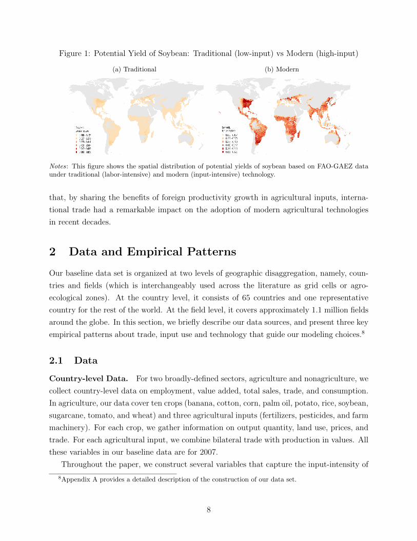
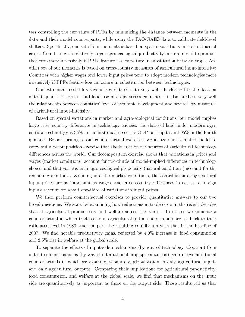
Figure 1: Potential Yield of Soybean: Traditional (low-input) vs Modern (high-input)

(a) Traditional (b) Modern

Notes: This figure shows the spatial distribution of potential yields of soybean based on FAO-GAEZ dataunder traditional (labor-intensive) and modern (input-intensive) technology.

that, by sharing the benefits of foreign productivity growth in agricultural inputs, interna-

tional trade had a remarkable impact on the adoption of modern agricultural technologies

in recent decades.

2 Data and Empirical Patterns

Our baseline data set is organized at two levels of geographic disaggregation, namely, coun-

tries and fields (which is interchangeably used across the literature as grid cells or agro-

ecological zones). At the country level, it consists of 65 countries and one representative

country for the rest of the world. At the field level, it covers approximately 1.1 million fields

around the globe. In this section, we briefly describe our data sources, and present three key

empirical patterns about trade, input use and technology that guide our modeling choices.8

2.1 Data

Country-level Data. For two broadly-defined sectors, agriculture and nonagriculture, we

collect country-level data on employment, value added, total sales, trade, and consumption.

In agriculture, our data cover ten crops (banana, cotton, corn, palm oil, potato, rice, soybean,

sugarcane, tomato, and wheat) and three agricultural inputs (fertilizers, pesticides, and farm

machinery). For each crop, we gather information on output quantity, land use, prices, and

trade. For each agricultural input, we combine bilateral trade with production in values. All

these variables in our baseline data are for 2007.

Throughout the paper, we construct several variables that capture the input-intensity of

8Appendix A provides a detailed description of the construction of our data set.

8

agriculture across countries. In particular, we measure cost share of inputs in agriculture (i.e.

expenditure on inputs divided by gross output in agriculture), labor-per-land, and fertilizer-

per-land measured as tonnes of fertilizer use divided by total cropland. In addition to our

baseline data in 2007, we assemble trade and gross output data for 1980 which we use later

to measure changes in trade costs and productivity between 1980 and 2007.

Field-level data. A field corresponds to an agro-ecological zone (AEZ) as a 5 min by 5

min latitude/longitude grid cell encompassing an area of approximately 10 by 10 km. For

each field, we collect information from the Food and Agriculture Organization’s Global Agro-

Ecological Zones (FAO-GAEZ) project, which reports attainable output per unit of land, in

tonnes per hectare, if the entire field were allocated to a crop and a given technology were

used. These measures of agricultural suitability, reported by crops and types of technology,

are referred to as “potential yields”. These measures are generated by agronomic models that

exploit field-level information on agro-ecological characteristics, such as soil types, elevation,

rainfall and temperature, under the assumption that the same economic conditions hold in

all fields around the world.

We bring in, for each crop, data on potential yields for two technology types. First, a

low-input technology that corresponds to traditional farming activities where production is

labor-intensive and there is no use of agricultural inputs. Second, a high-input technology

that corresponds to modern systems where production is intensive in the use of agricultural

machinery and applications of nutrients and chemical pest, disease and weed control. Here-

after, we call low- and high-input technologies, respectively, “traditional” and “modern”.9

Figure 1 plots potential yields of soybean based on traditional and modern technologies

across the world geography.

Lastly, we use data on the total share of cropland in every field around the world from

Earthstat. These data are generated by land-classification models that take satellite imagery

as inputs.10

9According to FAO-GAEZ, the low-input technology represents a production technology with“no applica-tion of nutrients, no use of chemicals for pest and disease control” and the high-input production technologyis “fully mechanized with low labor intensity and uses optimum applications of nutrients and chemical pest,disease and weed control.” In addition, FAO-GAEZ reports potential yields based on an intermediate inputintensity, which we do not use in this paper.

10The EarthStat project is a collaboration between the Global Landscapes Initiative at the University ofMinnesota’s Institute on the Environment and the Land Use and Global Environment Lab at the Universityof British Columbia.

9

2.2 Empirical Patterns

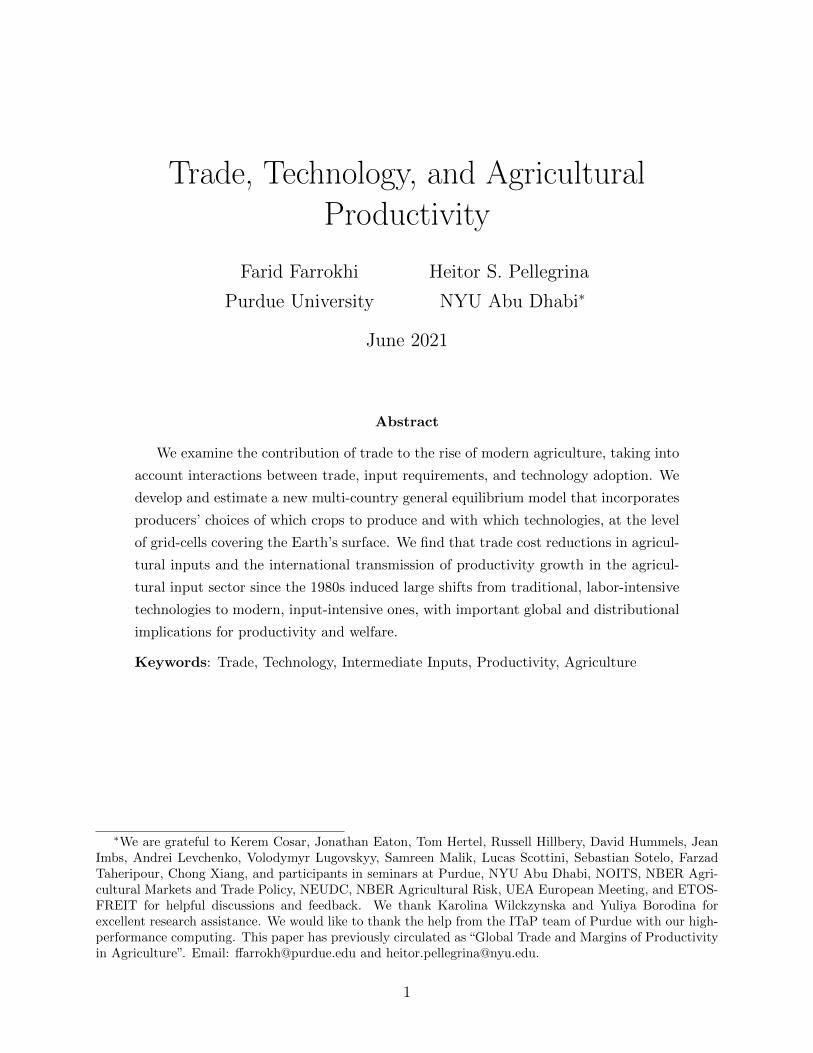
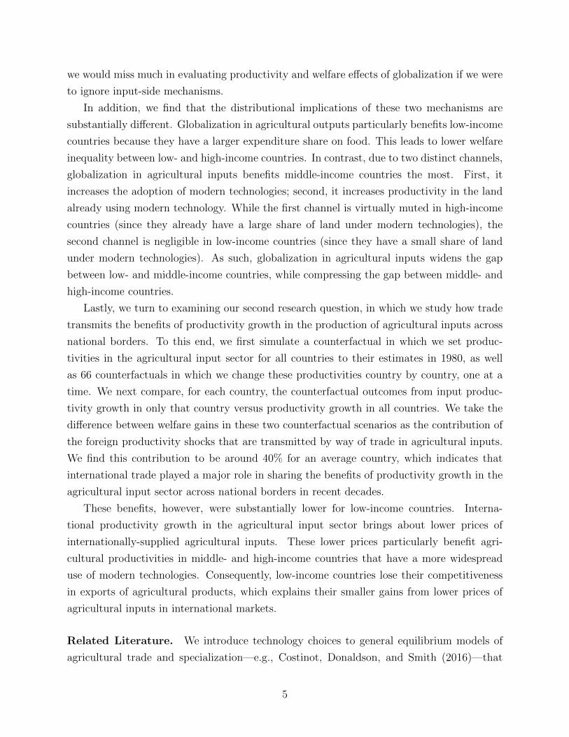
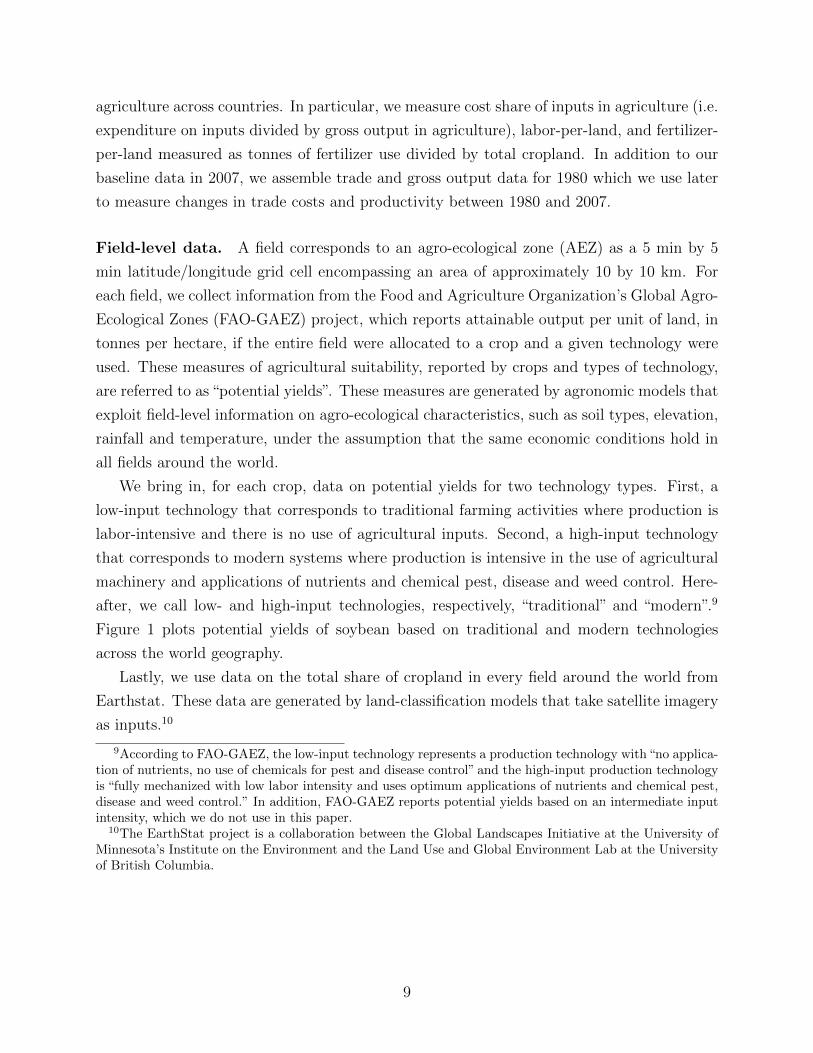
Pattern 1. Across countries, cost share of agricultural inputs and input-per-land

or per-labor rise with GDP per capita, whereas labor-per-land falls with GDP

per capita. A key feature of economic development is that input use in agriculture rises

markedly with GDP per capita (e.g. See Restuccia, Yang, and Zhu (2008b), Gollin, Parente,

and Rogerson (2007) and Donovan (2017)). Figure 2 revisits these patterns in our data.

Panel (a) shows that the cost share of agricultural inputs rises with GDP per capita: It is

approximately 25 and 60 percent respectively in the first and fourth quartile of GDP per

capita. Panels (b)-(c)-(d) show the scatter plot of labor-per-land, fertilizer-per-land, and

fertilizer-per-labor in agriculture against GDP per capita. Countries with higher GDP per

capita use fertilizers more intensively relative to land or labor, whereas they save on labor

per unit of land.

Given these striking cuts of data, we develop a model that is designed to generate techno-

logical differences in agricultural production across countries as an endogenous outcome. For

instance, in a country where wages are low, or input prices are high, agricultural producers

will have incentives to choose traditional, labor-intensive technologies rather than modern,

input-intensive ones.

Pattern 2. Across countries, the import share of agricultural inputs is typically

large, and exports of agricultural inputs are concentrated in a relatively small

number of countries. Given the strong relationship between agricultural input-intensity

and economic development that we presented in Pattern 1, we now ask how much countries

rely on international trade to procure agricultural inputs. Table 1 shows that the import

share of all agricultural inputs combined is typically large, with an average of 0.65 across

countries in 2007. It also indicates substantial cross-country heterogeneity in import shares

for different inputs: for example, the import share of fertilizers range between 0.36 at the

10th percentile and 0.97 at the 90th percentile. Most countries, in fact, largely depend on

international trade to procure at least one of fertilizers, pesticides, or farm machinery. This

reflects the high geographic concentration in the production of agricultural inputs. The ten

largest exporting countries account for approximately 80% of all the international exports of

agricultural inputs. As shown in Table A.1 in the Online Appendix, fertilizer production is

concentrated in several countries that have the required natural resources, and the production

of pesticides and farm machinery requires chemical- and machinery-related technologies that

might be unavailable to low-income countries.11

11For instance, countries in the Middle East and North Africa (MENA) and in the East Europe have largeendowments of raw fertilizers, and, therefore, present a small import share of fertilizers, but imports in these

10

Figure 2: Cross-Country relationships between Cost Share of Inputs in Agriculture, InputUse and GDP per capita (2007)

(a) Cost share of Agricultural Inputs

ALB

ARG

AUSAUT

BFABGD

BRA

CAN

CHLCHN

CIVCMR

COG

COL

CRI

CZEDEU

DOM

DZA

ECUEGYESP

ETH

FIN

FRAGBR

GHA

GRC

HUN

IDNIND

IRN

ITA

JPN

KEN

KOR

LKA

MARMEX

MLI

MOZ

MYS

NLD NORNZL

PAK

PERPHL

POL

PRT

PRY

ROU

ROWSEN

SOV

SWE

THATUN TUR

TZA

URY

USAVEN

VNM

YUGZAF

0.2

.4.6

.8C

ost s

hare

of a

gric

ultu

ral i

nput

s

−4 −3 −2 −1 0 1Log GDP per worker

R2 = 0.68 and slope = 0.09

(b) Labor per Land

ALB

ARG

AUS

AUT

BFA

BGD

BRA

CAN

CHL

CHN

CIVCMR

COG COL

CRI

CZE DEU

DOM

DZA

ECU

EGY

ESP

ETH

FINFRAGBR

GHA

GRC

HUN

IDN

IND

IRN

ITA

JPN

KEN

KOR

LKA

MAR

MEX

MLI

MOZ

MYS NLD

NOR

NZL

PAKPER

PHL

POLPRT

PRYROU

ROW

SEN

SOV

SWE

THA

TUN

TUR

TZA

URY

USA

VEN

VNM

YUG

ZAF

−2

02

46

Labo

r / t

otal

agr

icul

tura

l lan

d


R2 = 0.58 and slope = −.82

(c) Fertilizer per Land

ALBARG AUS

AUT

BFA

BGD BRA

CAN

CHL

CHN

CIVCMR

COG

COL

CRI

CZE

DEU

DOM

DZA

ECU

EGY

ESP

ETH

FIN

FRAGBR

GHA

GRCHUNIDN

INDIRN

ITA

JPN

KEN

KOR

LKA

MARMEX

MLI

MOZ

MYS NLDNOR

NZL

PAKPERPHL

POLPRT

PRY

ROU

ROW

SEN

SOV

SWETHA

TUN

TUR

TZA

URY USAVEN

VNM

YUG

ZAF

−6

−4

−2

02

Fer

tiliz

er /

tota

l agr

icul

tura

l lan

d


R2 = 0.33 and slope = .662

(d) Fertilizer per Labor

ALB

ARG

AUS

AUT

BFA

BGD

BRA

CAN

CHLCHN

CIVCMR

COG

COL

CRI

CZE

DEU

DOM

DZA

ECUEGY

ESP

ETH

FINFRAGBR

GHA

GRC

HUN

IDNIND

IRN

ITA

JPN

KEN

KOR

LKA MAR

MEX

MLI

MOZ

MYS NLD

NOR

NZL

PAK PER

PHL

POL

PRTPRY

ROUROW

SEN

SOV

SWE

THATUN

TUR

TZA

URY

USA

VEN

VNM

YUGZAF

−10

−5

0F

ertil

izer

/ La

bor


R2 = 0.75 and slope = 1.48

Notes: This figure plots measures of agricultural input and labor intensity against GDP per capita ofcountries. Panel (a) shows input cost share, as measured by expenditure on inputs relative to gross output inagriculture. Panel (b) to (d) show fertilizer-per-land, labor-per-land, and fertilizer-per-labor where“fertilizer”is aggregate tonnes of fertilizer use, “land” is the cropland, and“labor” is the labor employment in agriculture.

Motivated by the important role of trade in the use of agricultural inputs (documented

in Table 1), in our framework we let countries purchase agricultural inputs domestically and

also from international suppliers. This will allow us to examine the importance of trade in

intermediate inputs for the adoption of input-intensive agricultural technologies.

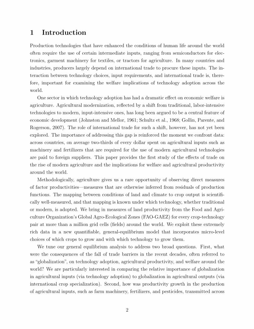
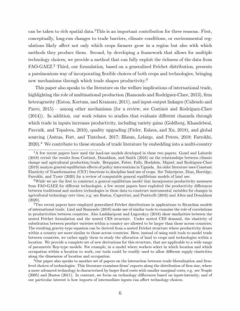
Pattern 3. Potential yields of modern technologies over traditional ones are large,

vary substantially across fields, and do not vary systematically across countries

with different GDP per capita. Figure 4 (a) shows the global average of the modern

countries account for a large share of their expenditure on farm machinery and pesticides. Import sharesof all the input categories are typically the largest among Sub-Saharan African countries and the lowest inNorth America and East Asia & Pacific. For most European and Latin American countries imports accountfor about a half of their expenditure on agricultural inputs.

11

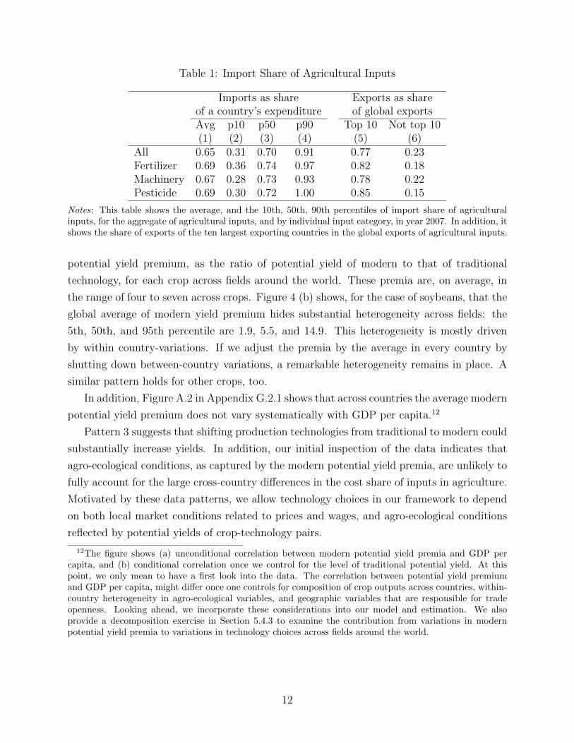
Table 1: Import Share of Agricultural Inputs

Imports as share Exports as shareof a country’s expenditure of global exportsAvg p10 p50 p90 Top 10 Not top 10(1) (2) (3) (4) (5) (6)

All 0.65 0.31 0.70 0.91 0.77 0.23Fertilizer 0.69 0.36 0.74 0.97 0.82 0.18Machinery 0.67 0.28 0.73 0.93 0.78 0.22Pesticide 0.69 0.30 0.72 1.00 0.85 0.15

Notes: This table shows the average, and the 10th, 50th, 90th percentiles of import share of agriculturalinputs, for the aggregate of agricultural inputs, and by individual input category, in year 2007. In addition, itshows the share of exports of the ten largest exporting countries in the global exports of agricultural inputs.

potential yield premium, as the ratio of potential yield of modern to that of traditional

technology, for each crop across fields around the world. These premia are, on average, in

the range of four to seven across crops. Figure 4 (b) shows, for the case of soybeans, that the

global average of modern yield premium hides substantial heterogeneity across fields: the

5th, 50th, and 95th percentile are 1.9, 5.5, and 14.9. This heterogeneity is mostly driven

by within country-variations. If we adjust the premia by the average in every country by

shutting down between-country variations, a remarkable heterogeneity remains in place. A

similar pattern holds for other crops, too.

In addition, Figure A.2 in Appendix G.2.1 shows that across countries the average modern

potential yield premium does not vary systematically with GDP per capita.12

Pattern 3 suggests that shifting production technologies from traditional to modern could

substantially increase yields. In addition, our initial inspection of the data indicates that

agro-ecological conditions, as captured by the modern potential yield premia, are unlikely to

fully account for the large cross-country differences in the cost share of inputs in agriculture.

Motivated by these data patterns, we allow technology choices in our framework to depend

on both local market conditions related to prices and wages, and agro-ecological conditions

reflected by potential yields of crop-technology pairs.

12The figure shows (a) unconditional correlation between modern potential yield premia and GDP percapita, and (b) conditional correlation once we control for the level of traditional potential yield. At thispoint, we only mean to have a first look into the data. The correlation between potential yield premiumand GDP per capita, might differ once one controls for composition of crop outputs across countries, within-country heterogeneity in agro-ecological variables, and geographic variables that are responsible for tradeopenness. Looking ahead, we incorporate these considerations into our model and estimation. We alsoprovide a decomposition exercise in Section 5.4.3 to examine the contribution from variations in modernpotential yield premia to variations in technology choices across fields around the world.

12

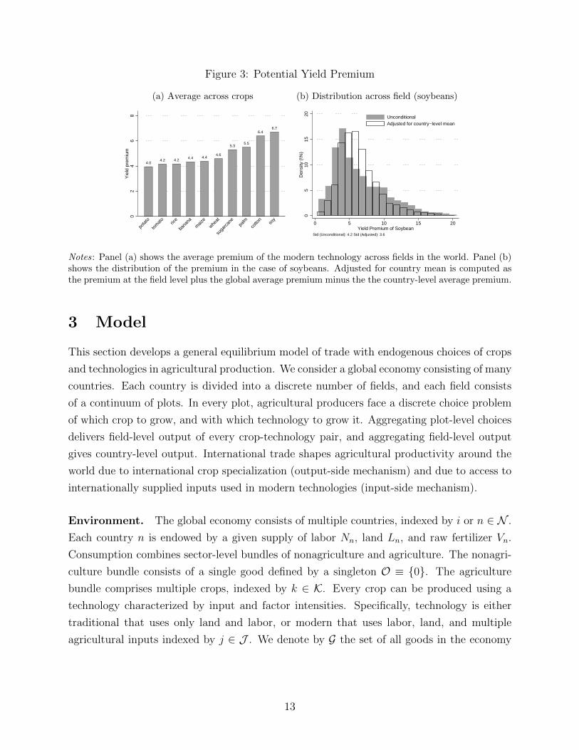
Figure 3: Potential Yield Premium

(a) Average across crops

4.04.2 4.2 4.4 4.4

4.6

5.35.5

6.46.7

02

46

8Y

ield

pre

miu

m

pota

to

tom

ato

rice

bana

na

maiz

e

wheat

suga

rcan

epa

lmco

tton

soy

(b) Distribution across field (soybeans)

05

1015

20D

ensi

ty (

\%)

0 5 10 15 20Yield Premium of Soybean

UnconditionalAdjusted for country−level mean

Std (Unconditional): 4.2 Std (Adjusted): 3.6

Notes: Panel (a) shows the average premium of the modern technology across fields in the world. Panel (b)shows the distribution of the premium in the case of soybeans. Adjusted for country mean is computed asthe premium at the field level plus the global average premium minus the the country-level average premium.

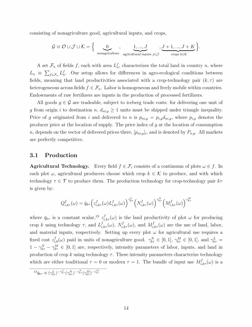
3 Model

This section develops a general equilibrium model of trade with endogenous choices of crops

and technologies in agricultural production. We consider a global economy consisting of many

countries. Each country is divided into a discrete number of fields, and each field consists

of a continuum of plots. In every plot, agricultural producers face a discrete choice problem

of which crop to grow, and with which technology to grow it. Aggregating plot-level choices

delivers field-level output of every crop-technology pair, and aggregating field-level output

gives country-level output. International trade shapes agricultural productivity around the

world due to international crop specialization (output-side mechanism) and due to access to

internationally supplied inputs used in modern technologies (input-side mechanism).

Environment. The global economy consists of multiple countries, indexed by i or n ∈ N .

Each country n is endowed by a given supply of labor Nn, land Ln, and raw fertilizer Vn.

Consumption combines sector-level bundles of nonagriculture and agriculture. The nonagri-

culture bundle consists of a single good defined by a singleton O ≡ 0. The agriculture

bundle comprises multiple crops, indexed by k ∈ K. Every crop can be produced using a

technology characterized by input and factor intensities. Specifically, technology is either

traditional that uses only land and labor, or modern that uses labor, land, and multiple

agricultural inputs indexed by j ∈ J . We denote by G the set of all goods in the economy

13

consisting of nonagriculture good, agricultural inputs, and crops,

G ≡ O ∪ J ∪ K =

0︸︷︷︸nonagriculture

, 1, ..., J︸︷︷︸agricultural inputs j∈J

, J + 1, ..., J +K︸︷︷︸crops k∈K

.

A set Fn of fields f , each with area Lfn, characterizes the total land in country n, where

Ln ≡∑

f∈Fn Lfn. Our setup allows for differences in agro-ecological conditions between

fields, meaning that land productivities associated with a crop-technology pair (k, τ) are

heterogeneous across fields f ∈ Fn. Labor is homogeneous and freely mobile within countries.

Endowments of raw fertilizers are inputs in the production of processed fertilizers.

All goods g ∈ G are tradeable, subject to iceberg trade costs: for delivering one unit of

g from origin i to destination n, dni,g ≥ 1 units must be shipped under triangle inequality.

Price of g originated from i and delivered to n is pni,g = pi,gdni,g, where pi,g denotes the

producer price at the location of supply. The price index of g at the location of consumption

n, depends on the vector of delivered prices there, [pni,g]i, and is denoted by Pn,g. All markets

are perfectly competitive.

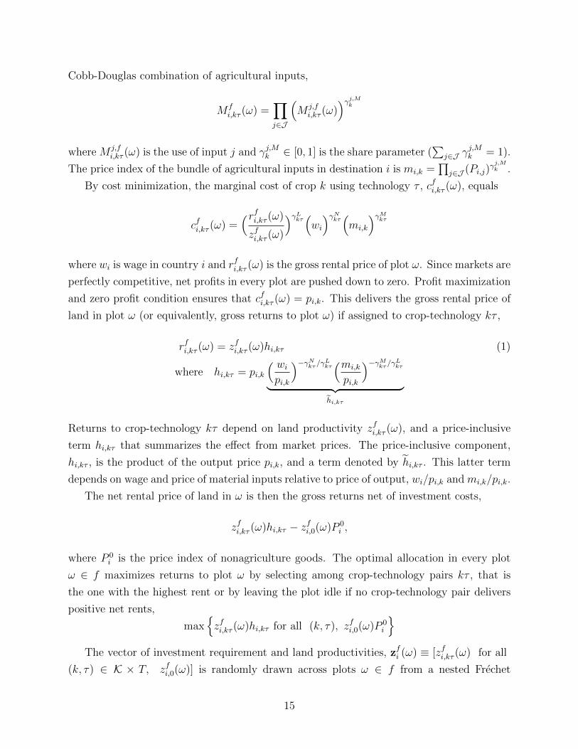
3.1 Production

Agricultural Technology. Every field f ∈ Fi consists of a continuum of plots ω ∈ f . In

each plot ω, agricultural producers choose which crop k ∈ K to produce, and with which

technology τ ∈ T to produce them. The production technology for crop-technology pair kτ

is given by:

Qfi,kτ (ω) = qkτ

(zfi,kτ (ω)Lfi,kτ (ω)

)γLkτ(N fi,kτ (ω)

)γNkτ(M f

i,kτ (ω))γMkτ

where qkτ is a constant scalar,13 zfi,kτ (ω) is the land productivity of plot ω for producing

crop k using technology τ , and Lfi,kτ (ω), N fi,kτ (ω), and M f

i,kτ (ω) are the use of land, labor,

and material inputs, respectively. Setting up every plot ω for agricultural use requires a

fixed cost zfi,0(ω) paid in units of nonagriculture good. γNkτ ∈ [0, 1], γMkτ ∈ [0, 1], and γLkτ =

1 − γNkτ − γMkτ ∈ [0, 1] are, respectively, intensity parameters of labor, inputs, and land in

production of crop k using technology τ . These intensity parameters characterize technology

which are either traditional τ = 0 or modern τ = 1. The bundle of input use M fi,kτ (ω) is a

13qkτ ≡ (γLkτ )−γLkτ (γNkτ )−γ

Nkτ (γMkτ )−γ

Mkτ

14

Cobb-Douglas combination of agricultural inputs,

M fi,kτ (ω) =

∏j∈J

(M j,f

i,kτ (ω))γj,Mk

where M j,fi,kτ (ω) is the use of input j and γj,Mk ∈ [0, 1] is the share parameter (

∑j∈J γ

j,Mk = 1).

The price index of the bundle of agricultural inputs in destination i is mi,k =∏

j∈J (Pi,j)γj,Mk .

By cost minimization, the marginal cost of crop k using technology τ , cfi,kτ (ω), equals

cfi,kτ (ω) =(rfi,kτ (ω)

zfi,kτ (ω)

)γLkτ(wi

)γNkτ(mi,k

)γMkτwhere wi is wage in country i and rfi,kτ (ω) is the gross rental price of plot ω. Since markets are

perfectly competitive, net profits in every plot are pushed down to zero. Profit maximization

and zero profit condition ensures that cfi,kτ (ω) = pi,k. This delivers the gross rental price of

land in plot ω (or equivalently, gross returns to plot ω) if assigned to crop-technology kτ ,

rfi,kτ (ω) = zfi,kτ (ω)hi,kτ (1)

where hi,kτ = pi,k

( wipi,k

)−γNkτ/γLkτ(mi,k

pi,k

)−γMkτ/γLkτ︸︷︷︸

hi,kτ

Returns to crop-technology kτ depend on land productivity zfi,kτ (ω), and a price-inclusive

term hi,kτ that summarizes the effect from market prices. The price-inclusive component,

hi,kτ , is the product of the output price pi,k, and a term denoted by hi,kτ . This latter term

depends on wage and price of material inputs relative to price of output, wi/pi,k and mi,k/pi,k.

The net rental price of land in ω is then the gross returns net of investment costs,

zfi,kτ (ω)hi,kτ − zfi,0(ω)P 0i ,

where P 0i is the price index of nonagriculture goods. The optimal allocation in every plot

ω ∈ f maximizes returns to plot ω by selecting among crop-technology pairs kτ , that is

the one with the highest rent or by leaving the plot idle if no crop-technology pair delivers

positive net rents,

maxzfi,kτ (ω)hi,kτ for all (k, τ), zfi,0(ω)P 0

i

The vector of investment requirement and land productivities, zfi (ω) ≡ [zfi,kτ (ω) for all

(k, τ) ∈ K × T, zfi,0(ω)] is randomly drawn across plots ω ∈ f from a nested Frechet

15

distribution,

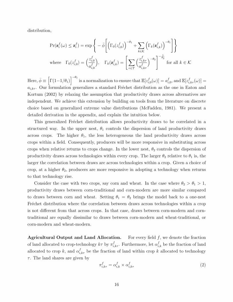
Pr(zfi (ω) ≤ zfi ) = exp

− φ

[(Γ0(zfi,0)

)−θ1+∑k∈K

(Γk(z

fi,k))−θ1]

where Γ0(zfi,0) =(zfi,0afi,0

), Γk(z

fi,k) =

[∑τ∈T

(zfi,kτafi,kτ

)−θ2]− 1θ2

for all k ∈ K

Here, φ ≡[Γ(1−1/θ1)

]−θ1is a normalization to ensure that E[zfi,0(ω)] = afi,0, and E[zfi,kτ (ω)] =

ai,kτ . Our formulation generalizes a standard Frechet distribution as the one in Eaton and

Kortum (2002) by relaxing the assumption that productivity draws across alternatives are

independent. We achieve this extension by building on tools from the literature on discrete

choice based on generalized extreme value distributions (McFadden, 1981). We present a

detailed derivation in the appendix, and explain the intuition below.

This generalized Frechet distribution allows productivity draws to be correlated in a

structured way. In the upper nest, θ1 controls the dispersion of land productivity draws

across crops. The higher θ1, the less heterogeneous the land productivity draws across

crops within a field. Consequently, producers will be more responsive in substituting across

crops when relative returns to crops change. In the lower nest, θ2 controls the dispersion of

productivity draws across technologies within every crop. The larger θ2 relative to θ1 is, the

larger the correlation between draws are across technologies within a crop. Given a choice of

crop, at a higher θ2, producers are more responsive in adopting a technology when returns

to that technology rise.

Consider the case with two crops, say corn and wheat. In the case where θ2 > θ1 > 1,

productivity draws between corn-traditional and corn-modern are more similar compared

to draws between corn and wheat. Setting θ1 = θ2 brings the model back to a one-nest

Frechet distribution where the correlation between draws across technologies within a crop

is not different from that across crops. In that case, draws between corn-modern and corn-

traditional are equally dissimilar to draws between corn-modern and wheat-traditional, or

corn-modern and wheat-modern.

Agricultural Output and Land Allocation. For every field f , we denote the fraction

of land allocated to crop-technology kτ by πfi,kτ . Furthermore, let αfi,k be the fraction of land

allocated to crop k, and αfi,kτ be the fraction of land within crop k allocated to technology

τ . The land shares are given by

πfi,kτ = αfi,k × αfi,kτ (2)

16

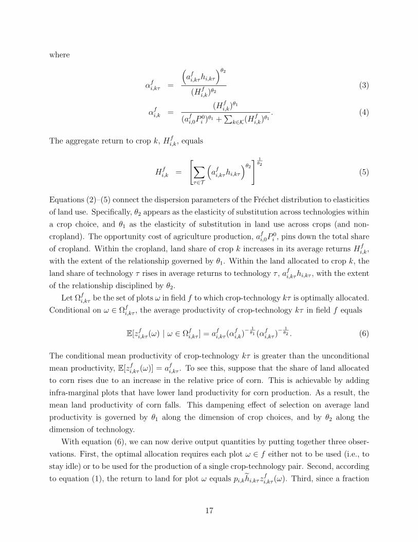
where

αfi,kτ =

(afi,kτhi,kτ

)θ2(Hf

i,k)θ2

(3)

αfi,k =(Hf

i,k)θ1

(afi,0P0i )θ1 +

∑k∈K(Hf

i,k)θ1. (4)

The aggregate return to crop k, Hfi,k, equals

Hfi,k =

[∑τ∈T

(afi,kτhi,kτ

)θ2] 1θ2

(5)

Equations (2)–(5) connect the dispersion parameters of the Frechet distribution to elasticities

of land use. Specifically, θ2 appears as the elasticity of substitution across technologies within

a crop choice, and θ1 as the elasticity of substitution in land use across crops (and non-

cropland). The opportunity cost of agriculture production, afi,0P0i , pins down the total share

of cropland. Within the cropland, land share of crop k increases in its average returns Hfi,k,

with the extent of the relationship governed by θ1. Within the land allocated to crop k, the

land share of technology τ rises in average returns to technology τ , afi,kτhi,kτ , with the extent

of the relationship disciplined by θ2.

Let Ωfi,kτ be the set of plots ω in field f to which crop-technology kτ is optimally allocated.

Conditional on ω ∈ Ωfi,kτ , the average productivity of crop-technology kτ in field f equals

E[zfi,kτ (ω) | ω ∈ Ωfi,kτ ] = afi,kτ (α

fi,k)− 1θ1 (αfi,kτ )

− 1θ2 . (6)

The conditional mean productivity of crop-technology kτ is greater than the unconditional

mean productivity, E[zfi,kτ (ω)] = afi,kτ . To see this, suppose that the share of land allocated

to corn rises due to an increase in the relative price of corn. This is achievable by adding

infra-marginal plots that have lower land productivity for corn production. As a result, the

mean land productivity of corn falls. This dampening effect of selection on average land

productivity is governed by θ1 along the dimension of crop choices, and by θ2 along the

dimension of technology.

With equation (6), we can now derive output quantities by putting together three obser-

vations. First, the optimal allocation requires each plot ω ∈ f either not to be used (i.e., to

stay idle) or to be used for the production of a single crop-technology pair. Second, according

to equation (1), the return to land for plot ω equals pi,khi,kτzfi,kτ (ω). Third, since a fraction

17

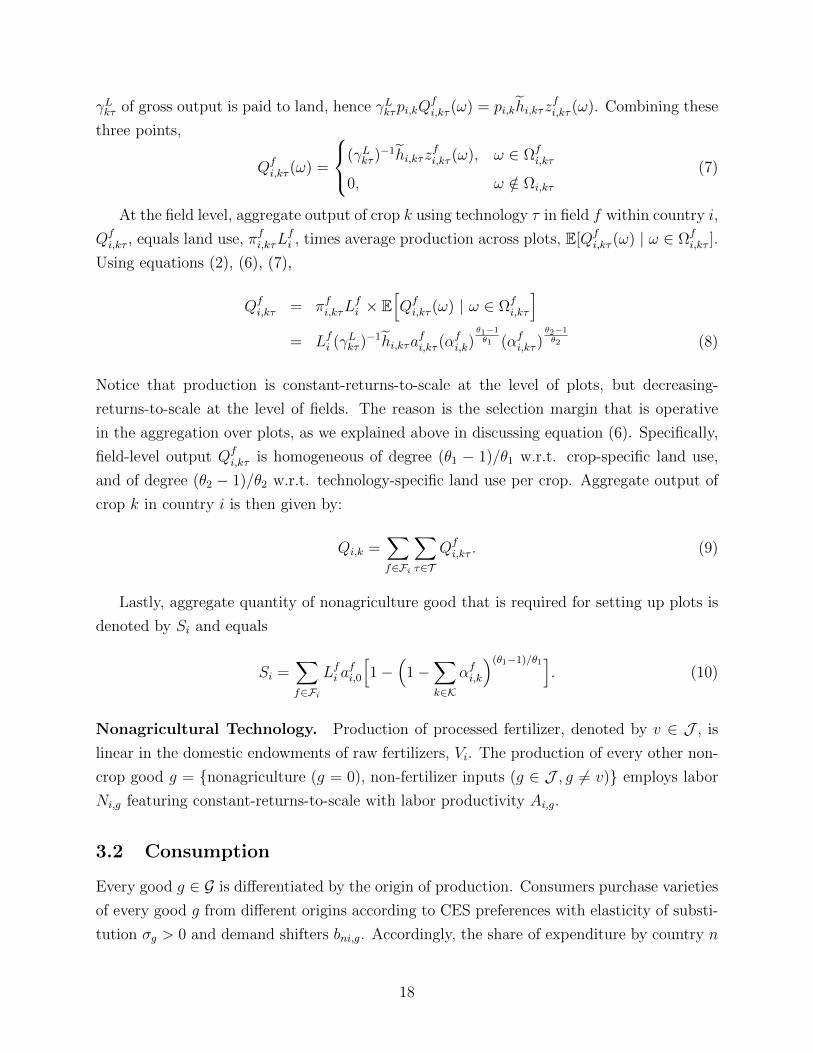
γLkτ of gross output is paid to land, hence γLkτpi,kQfi,kτ (ω) = pi,khi,kτz

fi,kτ (ω). Combining these

three points,

Qfi,kτ (ω) =

(γLkτ )−1hi,kτz

fi,kτ (ω), ω ∈ Ωf

i,kτ

0, ω /∈ Ωi,kτ

(7)

At the field level, aggregate output of crop k using technology τ in field f within country i,

Qfi,kτ , equals land use, πfi,kτL

fi , times average production across plots, E[Qf

i,kτ (ω) | ω ∈ Ωfi,kτ ].

Using equations (2), (6), (7),

Qfi,kτ = πfi,kτL

fi × E

[Qfi,kτ (ω) | ω ∈ Ωf

i,kτ

]= Lfi (γ

Lkτ )−1hi,kτa

fi,kτ (α

fi,k)

θ1−1θ1 (αfi,kτ )

θ2−1θ2 (8)

Notice that production is constant-returns-to-scale at the level of plots, but decreasing-

returns-to-scale at the level of fields. The reason is the selection margin that is operative

in the aggregation over plots, as we explained above in discussing equation (6). Specifically,

field-level output Qfi,kτ is homogeneous of degree (θ1 − 1)/θ1 w.r.t. crop-specific land use,

and of degree (θ2 − 1)/θ2 w.r.t. technology-specific land use per crop. Aggregate output of

crop k in country i is then given by:

Qi,k =∑f∈Fi

∑τ∈T

Qfi,kτ . (9)

Lastly, aggregate quantity of nonagriculture good that is required for setting up plots is

denoted by Si and equals

Si =∑f∈Fi

Lfi afi,0

[1−

(1−

∑k∈K

αfi,k

)(θ1−1)/θ1]. (10)

Nonagricultural Technology. Production of processed fertilizer, denoted by v ∈ J , is

linear in the domestic endowments of raw fertilizers, Vi. The production of every other non-

crop good g = nonagriculture (g = 0), non-fertilizer inputs (g ∈ J , g 6= v) employs labor

Ni,g featuring constant-returns-to-scale with labor productivity Ai,g.

3.2 Consumption

Every good g ∈ G is differentiated by the origin of production. Consumers purchase varieties

of every good g from different origins according to CES preferences with elasticity of substi-

tution σg > 0 and demand shifters bni,g. Accordingly, the share of expenditure by country n

18

on good g ∈ G from origin i is:

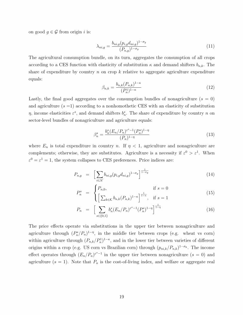
λni,g =bni,g(pi,gdni,g)

1−σg

(Pn,g)1−σg(11)

The agricultural consumption bundle, on its turn, aggregates the consumption of all crops

according to a CES function with elasticity of substitution κ and demand shifters bn,k. The

share of expenditure by country n on crop k relative to aggregate agriculture expenditure

equals:

βn,k =bn,k(Pn,k)

1−κ

(P 1n)1−κ (12)

Lastly, the final good aggregates over the consumption bundles of nonagriculture (s = 0)

and agriculture (s =1) according to a nonhomothetic CES with an elasticity of substitution

η, income elasticities εs, and demand shifters bsn. The share of expenditure by country n on

sector-level bundles of nonagriculture and agriculture equals:

βsn =bsn(En/Pn)ε

s−1(P sn)1−η

(Pn)1−η (13)

where En is total expenditure in country n. If η < 1, agriculture and nonagriculture are

complements; otherwise, they are substitutes. Agriculture is a necessity if ε0 > ε1. When

ε0 = ε1 = 1, the system collapses to CES preferences. Price indices are:

Pn,g =[∑i∈N

bni,g(pi,gdni,g)1−σg

] 11−σg

(14)

P sn =

Pn,0, if s = 0[∑k∈K bn,k(Pn,k)

1−κ] 1

1−κ, if s = 1

(15)

Pn =[ ∑s∈0,1

bsn(En/Pn)εs−1(P s

n)1−η] 1

1−η(16)

The price effects operate via substitutions in the upper tier between nonagriculture and

agriculture through (P sn/Pn)1−η, in the middle tier between crops (e.g. wheat vs corn)

within agriculture through (Pn,k/P1n)1−κ, and in the lower tier between varieties of different

origins within a crop (e.g. US corn vs Brazilian corn) through (pni,k/Pn,k)1−σk . The income

effect operates through (En/Pn)εs−1 in the upper tier between nonagriculture (s = 0) and

agriculture (s = 1). Note that Pn is the cost-of-living index, and welfare or aggregate real

19

consumption thus equals Cn = En/Pn.14

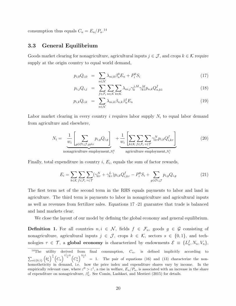
3.3 General Equilibrium

Goods market clearing for nonagriculture, agricultural inputs j ∈ J , and crops k ∈ K require

supply at the origin country to equal world demand,

pi,0Qi,0 =∑n∈N

λni,0β0nEn + P 0

i Si (17)

pi,jQi,j =∑f∈Fi

∑n∈N

∑k∈K

λni,jγj,Mk γMk1pn,kQ

fn,k1 (18)

pi,kQi,k =∑n∈N

λni,kβn,kβ1nEn (19)

Labor market clearing in every country i requires labor supply Ni to equal labor demand

from agriculture and elsewhere,

Ni =1

wi

[ ∑g∈O∪J ,g 6=v

pi,gQi,g

]︸︷︷︸

nonagriculture employment,N0i

+1

wi

[∑k∈K

∑f∈Fi

∑τ∈T

γNkτpi,kQfi,kτ

]︸︷︷︸

agriculture employment,N1i

(20)

Finally, total expenditure in country i, Ei, equals the sum of factor rewards,

Ei =∑k∈K

∑f∈Fi

∑τ∈T

(γNkτ + γLkτ )pi,kQfi,kτ − P

0i Si +

∑g∈O∪J

pi,gQi,g (21)

The first term net of the second term in the RHS equals payments to labor and land in

agriculture. The third term is payments to labor in nonagriculture and agricultural inputs

as well as revenues from fertilizer sales. Equations 17 -21 guarantee that trade is balanced

and land markets clear.

We close the layout of our model by defining the global economy and general equilibrium.

Definition 1. For all countries n, i ∈ N , fields f ∈ Fn, goods g ∈ G consisting of

nonagriculture, agricultural inputs j ∈ J , crops k ∈ K, sectors s ∈ 0, 1, and tech-

nologies τ ∈ T , a global economy is characterized by endowments E ≡ Lfn, Nn, Vn,14The utility derived from final consumption, Cn, is defined implicitly according to∑s∈0,1

(bsn

) 1η(Cn

) εs−ηη(Csn

) η−1η

= 1. The pair of equations (16) and (13) characterize the non-

homotheticity in demand, i.e. how the price index and expenditure shares vary by income. In theempirically relevant case, where ε0 > ε1, a rise in welfare, En/Pn, is associated with an increase in the shareof expenditure on nonagriculture, β1

n. See Comin, Lashkari, and Mestieri (2015) for details.

20

supply parameters ΩS ≡ θ1, θ2, γLkτ , γ

Mkτ , γ

Nkτ , γ

j,Mk , afn,0, a

fn,kτ, and demand parameters

ΩD ≡ ε0, ε1, η, κ, σg, bsn, bn,k, bni,g, dni,g, An,g.15

Definition 2. Given a global economy characterized by E ,ΩS,ΩD, a general equilib-

rium consists of prices pn,g in all countries n ∈ N and for all goods g ∈ G, such that

equations 1–21 hold.

4 Discussion: Trade, Technology, and Productivity

This section discusses the interplay between trade, technology and agricultural productivity

in our model. First, we derive and discuss the production possibility frontiers (PPF) implied

by our generalized Frechet distribution, which will be critical for the strategy that we use

to bring our model to FAO-GAEZ data. Second, we show how our model generates a new

source of gains from trade that arises from the interaction between technology and trade

in intermediate inputs. In doing so, we benchmark our analytical result with Arkolakis,

Costinot, and Rodriguez-Clare (2012).16

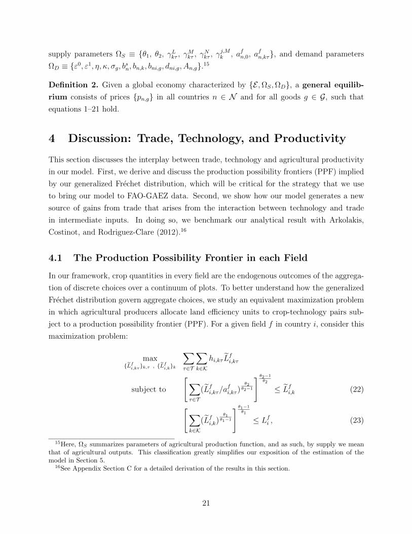
4.1 The Production Possibility Frontier in each Field

In our framework, crop quantities in every field are the endogenous outcomes of the aggrega-

tion of discrete choices over a continuum of plots. To better understand how the generalized

Frechet distribution govern aggregate choices, we study an equivalent maximization problem

in which agricultural producers allocate land efficiency units to crop-technology pairs sub-

ject to a production possibility frontier (PPF). For a given field f in country i, consider this

maximization problem:

maxLfi,kτk,τ , Lfi,kk

∑τ∈T

∑k∈K

hi,kτ Lfi,kτ

subject to

[∑τ∈T

(Lfi,kτ/afi,kτ )

θ2θ2−1

] θ2−1θ2

≤ Lfi,k (22)

[∑k∈K

(Lfi,k)θ1θ1−1

] θ1−1θ1

≤ Lfi , (23)

15Here, ΩS summarizes parameters of agricultural production function, and as such, by supply we meanthat of agricultural outputs. This classification greatly simplifies our exposition of the estimation of themodel in Section 5.

16See Appendix Section C for a detailed derivation of the results in this section.

21

where Lfi,kτ and Lfi,k are efficiency units of land at the level of crop-technology kτ , and crop k.

The agricultural producer maximizes the sum of returns across uses of land,∑

τ∈T∑

k∈K hi,kτ Lfi,kτ ,

subject to the PPF (equations 22, 23), i.e., she chooses Lfi,kτ and Lfi,k given price-inclusive

terms hi,kτ described by equation (1), technology coefficients afi,kτ , and land endowment Lfi .17

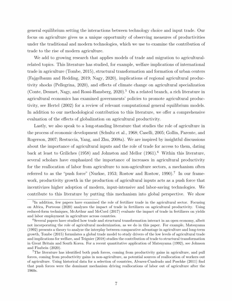
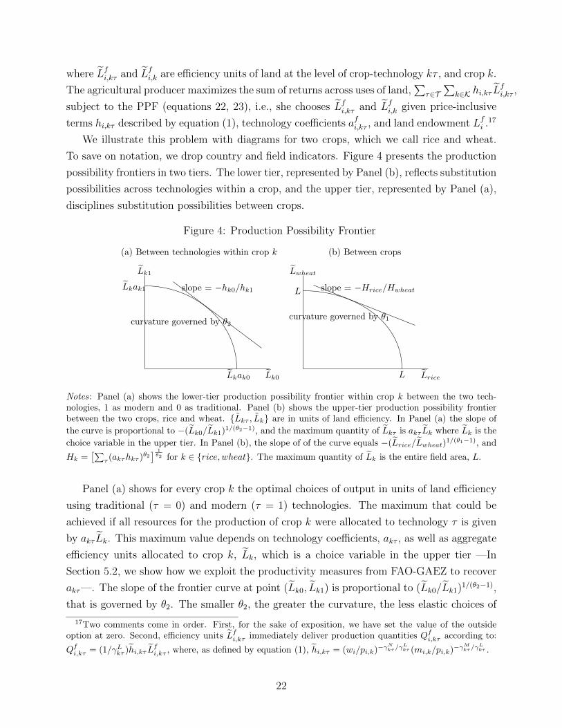
We illustrate this problem with diagrams for two crops, which we call rice and wheat.

To save on notation, we drop country and field indicators. Figure 4 presents the production

possibility frontiers in two tiers. The lower tier, represented by Panel (b), reflects substitution

possibilities across technologies within a crop, and the upper tier, represented by Panel (a),

disciplines substitution possibilities between crops.

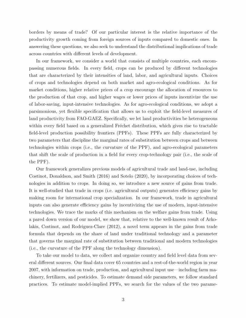
Figure 4: Production Possibility Frontier

(a) Between technologies within crop k

Lk0

Lk1

Lkak1

Lkak0

slope = −hk0/hk1

curvature governed by θ2

(b) Between crops

Lrice

Lwheat

slope = −Hrice/Hwheat

curvature governed by θ1

L

L

Notes: Panel (a) shows the lower-tier production possibility frontier within crop k between the two tech-nologies, 1 as modern and 0 as traditional. Panel (b) shows the upper-tier production possibility frontierbetween the two crops, rice and wheat. Lkτ , Lk are in units of land efficiency. In Panel (a) the slope of

the curve is proportional to −(Lk0/Lk1)1/(θ2−1), and the maximum quantity of Lkτ is akτ Lk where Lk is the

choice variable in the upper tier. In Panel (b), the slope of of the curve equals −(Lrice/Lwheat)1/(θ1−1), and

Hk =[∑

τ (akτhkτ )θ2] 1θ2 for k ∈ rice, wheat. The maximum quantity of Lk is the entire field area, L.

Panel (a) shows for every crop k the optimal choices of output in units of land efficiency

using traditional (τ = 0) and modern (τ = 1) technologies. The maximum that could be

achieved if all resources for the production of crop k were allocated to technology τ is given

by akτ Lk. This maximum value depends on technology coefficients, akτ , as well as aggregate

efficiency units allocated to crop k, Lk, which is a choice variable in the upper tier —In

Section 5.2, we show how we exploit the productivity measures from FAO-GAEZ to recover

akτ—. The slope of the frontier curve at point (Lk0, Lk1) is proportional to (Lk0/Lk1)1/(θ2−1),

that is governed by θ2. The smaller θ2, the greater the curvature, the less elastic choices of

17Two comments come in order. First, for the sake of exposition, we have set the value of the outsideoption at zero. Second, efficiency units Lfi,kτ immediately deliver production quantities Qfi,kτ according to:

Qfi,kτ = (1/γLkτ )hi,kτ Lfi,kτ , where, as defined by equation (1), hi,kτ = (wi/pi,k)−γ

Nkτ/γ

Lkτ (mi,k/pi,k)−γ

Mkτ/γ

Lkτ .

22

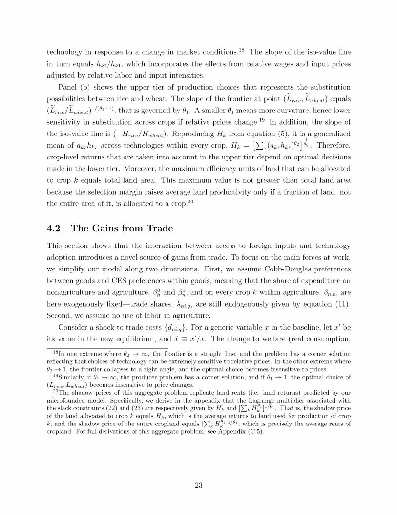
technology in response to a change in market conditions.18 The slope of the iso-value line

in turn equals hk0/hk1, which incorporates the effects from relative wages and input prices

adjusted by relative labor and input intensities.

Panel (b) shows the upper tier of production choices that represents the substitution

possibilities between rice and wheat. The slope of the frontier at point (Lrice, Lwheat) equals

(Lrice/Lwheat)1/(θ1−1), that is governed by θ1. A smaller θ1 means more curvature, hence lower

sensitivity in substitution across crops if relative prices change.19 In addition, the slope of

the iso-value line is (−Hrice/Hwheat). Reproducing Hk from equation (5), it is a generalized

mean of akτhkτ across technologies within every crop, Hk =[∑

τ (akτhkτ )θ2] 1θ2 . Therefore,

crop-level returns that are taken into account in the upper tier depend on optimal decisions

made in the lower tier. Moreover, the maximum efficiency units of land that can be allocated

to crop k equals total land area. This maximum value is not greater than total land area

because the selection margin raises average land productivity only if a fraction of land, not

the entire area of it, is allocated to a crop.20

4.2 The Gains from Trade

This section shows that the interaction between access to foreign inputs and technology

adoption introduces a novel source of gains from trade. To focus on the main forces at work,

we simplify our model along two dimensions. First, we assume Cobb-Douglas preferences

between goods and CES preferences within goods, meaning that the share of expenditure on

nonagriculture and agriculture, β0n and β1

n, and on every crop k within agriculture, βn,k, are

here exogenously fixed—trade shares, λni,g, are still endogenously given by equation (11).

Second, we assume no use of labor in agriculture.

Consider a shock to trade costs dni,g. For a generic variable x in the baseline, let x′ be

its value in the new equilibrium, and x ≡ x′/x. The change to welfare (real consumption,

18In one extreme where θ2 → ∞, the frontier is a straight line, and the problem has a corner solutionreflecting that choices of technology can be extremely sensitive to relative prices. In the other extreme whereθ2 → 1, the frontier collapses to a right angle, and the optimal choice becomes insensitive to prices.

19Similarly, if θ1 → ∞, the producer problem has a corner solution, and if θ1 → 1, the optimal choice of(Lrice, Lwheat) becomes insensitive to price changes.

20The shadow prices of this aggregate problem replicate land rents (i.e. land returns) predicted by ourmicrofounded model. Specifically, we derive in the appendix that the Lagrange multiplier associated withthe slack constraints (22) and (23) are respectively given by Hk and [

∑kH

θ1k ]1/θ1 . That is, the shadow price

of the land allocated to crop k equals Hk, which is the average returns to land used for production of cropk, and the shadow price of the entire cropland equals [

∑kH

θ1k ]1/θ1 , which is precisely the average rents of

cropland. For full derivations of this aggregate problem, see Appendix (C.5).

23

Ci) in response to changes to trade cost parameters (dni,g) becomes:

Ci =

(ρi,0

(λii,0

) 1σ0−1

)−β0i ∏

k

(ρi,k

(λii,k

) 1σk−1

)−β1i βi,k

︸︷︷︸nonag and ag trade (ACR)

[∑f

ρfi,k(αfi,k)

θ1−1θ1 (αfi,k0)

−1θ2

]β1i βi,k

︸︷︷︸ag productivity (New)

(24)

where ρi,0 and ρi,k are changes to value added share of nonagriculture and crop k, and ρfi,k is

the baseline value added share of field f within crop k. Equation (24) shows the sufficient set

of information required to calculate welfare gains from any change to trade costs. Notice that,

if all land is fully allocated to a single crop-technology pair, i.e., if αfi,k = αfi,k0 = 1, equation

(24) collapses to the standard formula for welfare change in a trade model with multiple-

sectors, as discussed in Costinot and Rodrıguez-Clare (2014). Here, changes to land shares

across crops and technologies is needed to calculate the change to real consumption.

Our welfare formula goes beyond previous formulas derived in the literature on input

trade, such as Blaum, Lelarge, and Peters (2018), in which input trade shares serve as a

sufficient statistic for the productivity gains from input trade. Suppose there is a single

agricultural input, indexed by M , whose production is linear in labor. The technology

margin in equation (24), i.e., (αfi,k0)−1θ2 , can then be expressed as:

(αfi,k0)−1θ2 =

[αfi,k0 + (1− αfi,k0)(vi,k)

θ2] 1θ2 , vi,k ≡

[(λii,M

) 1σM−1

(wipi,k

)]− 1−γLk,1γLk,1

where λii,M is the domestic share of expenditure on inputs, and (1−σM) is the corresponding

trade elasticity. The technology margin, (αfi,k0)−1θ2 , is a generalized mean between 1 and

vi,k, with their weights given by the baseline share of land under traditional and modern

technologies, αfi,k0 and αfi,k1 = 1−αfi,k0. In the special case of αfi,k0 = 1, the technology margin

becomes muted because agricultural production exclusively uses traditional technologies, in

which case αfi,k0 = 1. In the polar case of αfi,k0 = 0, agricultural production uses only modern

technologies, in which case λii,M is sufficient to know the technology margin—similar to

Blaum, Lelarge, and Peters (2018). In the general case of our model in which the two

technologies coexists, i.e., when αfi,k0 ∈ (0, 1), λii,M is insufficient to calculate the technology

margin, because one also needs knowledge of the baseline technology share, αfi,k0.

Lastly, to focus on the role of technology adoption, consider a pared down version of

our model in which utility solely depends on food consumption and agriculture consists of

a single crop.21 Consider also a country where agricultural inputs are entirely imported.

21We focus on the technology-related channel since the crop-related channel has been studied elsewhere.

24

This means that in autarky country i is restricted to domestic varieties for consumption,

and traditional technologies for production. In this stylized model, the gains from trade in

country i, defined as the percentage loss in real income from raising trade costs to infinity, is

Gi = 1− (λii)1

σ−1︸︷︷︸trade

(αi,0)1θ2︸︷︷︸

technology

, (25)

where λii is the baseline domestic share of expenditure on agriculture, and αi,0 is a weighted

average share of the domestic land allocated to traditional technology, αi,0 ≡[∑

f ρfi

(αfi,0

) 1θ2

]θ2.

Equation (25) underscores two sources of gains from trade: A classic channel, (λii)1

σ−1 , that

measures the gains from access to foreign consumption varieties, and a new channel, (αi,0)1θ2 ,

that reflects how access to foreign inputs unlocks the use of modern agricultural technolo-

gies. The gains from this new channel is summarized by the baseline share of land using the

traditional technology (αi,0), and the elasticity of substitution in production across technolo-

gies (θ2). The smaller αi,0 or θ2, the larger these gains. Compared to the classic one-sector

formula, i.e. Gi = 1 − (λii)1/(σ−1), equation (25) delivers unambiguously larger gains from

trade.

5 Taking the Model to Data

The estimation of our model consists of two steps. We first estimate demand-side parameters,

ΩD (for parameters included in ΩD, see Definition 1) using country-level data on produc-

tion and trade. We then estimate supply-side parameters of agriculture, ΩS, employing our

field-level data on potential yields and country-level data on agricultural production. After

presenting our estimation procedure, we discuss the identification of our supply side param-

eters. We then close this section by presenting the estimation results, model fit, and sources

of spatial variations in technology choices.

To see it, let θ2 →∞, then the agriculture productivity channel is given by:[∑f ρ

fi,k(αfi,k)

θ1−1θ1

]β1i βi,k

. This expression shows that a reallocation of land across crops matters for wel-

fare because θ1 is finite, meaning that crop production features decreasing returns to scale at the levelof fields. The analogue in the trade literature is where production features economies of scale and/or la-bor is imperfectly mobile across industries. For a recent discussion, see the gains from trade formula inKucheryavyy, Lyn, and Rodrıguez-Clare (2016), Galle, Rodrıguez-Clare, and Yi (2017), and Farrokhi andSoderbery (2020).

25

5.1 Demand-side parameters

Demand for Agricultural Goods. We estimate the demand for agricultural goods as

in Costinot, Donaldson, and Smith (2016). First, based on equation (11), we estimate the

elasticity of substitution between crop-varieties (σk) using:

log

(Xni,k

Xn,k

)= δn,k + (1− σk) log pi,k + εni,k.

Here, Xni,k is the purchases of n from country i of crop k, Xn,k is total purchases of coun-

try n of crop k, δn,k ≡ − log[∑

i bni,k(pi,kdni,k)1−σk ] is an importer-crop fixed effect, and

εni,k = log bni,kd1−σkni,k is a residual. We set

∑Ni=1 εni,k = 0 (without loss of generality), recover

bni,kd1−σkni,k from εni,k, and estimate a common elasticity of substitution between crop varieties

(σk = σ). Due to potential correlations between demand shocks and prices, we instrument

log pi,k with the average of potential yields across fields of the exporting country. With es-

timates of σk and bni,kd1−σkni,k , we construct Pn,k according to equation (15). Using equation

(12), we then estimate the elasticity of substitution between crops (κ) based on:

log(Xn,k

X1n

)= δn + (1− κ) logPn,k + εn,k,

where X1n is aggregate purchases of all crops, δn = (1 − κ) logP 1

n is a country fixed effect,

εn,k = log bn,k is a residual, and without loss of generality,∑

k∈K εn,k = 0. Again, to address

potential endogeneity issues, we instrument logPn,k using the average potential yield of each

pair of country-crop. We recover bn,k from residuals εn,k.

Demand for Nonagricultural Goods. We set σg = 4 for non-agriculture good and

for agricultural inputs based on the literature.22 For g = nonagriculture, pesticides, farm

machinery, we estimate:

log

(Xni,g

Xn,g

)− (1− σg) logwi = δn,g + δi,g + εni,g, (26)

where δn,g = (1− σg) logPn,g is a destination fixed effect, δi,g = (1− σg) logAi,g is an origin

fixed effect, and εni,g = log(bni,gd1−σgni,g ) is the residual. We recover bni,gd

1−σgni,g from εni,g and

Ai,g from δn,g. For g = fertilizers, we estimate the expression above without δi,g, substitute

logwi by log pi,g and recover bni,gd1−σgni,g from residuals.

22For example, see Simonovska and Waugh (2014) and Imbs and Mejean (2015).

26

Upper-tier Demand Parameters. We set income elasticities of nonagriculture and agri-

culture goods at ε0 = 1.5 and ε1 = 0.5, and the substitution elasticity between agriculture

and nonagriculture at η = 0.5 according to Comin, Lashkari, and Mestieri (2015).23 These

parameters imply that agriculture is a necessity whereas nonagriculture is a luxury, and

that agriculture and nonagriculture are complements. Given (η, ε0, ε1), we recover demand

shifters (b0n, b1

n) using expressions (16) and (13). To do so, we use model-implied price

indexes, (P 0n , P 1

n), which we obtain after fully calibrating the model.

5.2 Supply-Side Parameters

We now turn to the supply side parameters, ΩS. We define γL ≡ γL0 /γL1 and estimate

Θ = θ1, θ2, γL, subject to a calibration problem that sets Γ ≡ ΩS/Θ = afi,0, a

fi,kτ , γ

Nkτ ,

γLkτ , γMk , γj,Mk k,τ . Our estimation procedure can be thought of as a two-layer problem. In

the inner problem, we take Θ as given, and calibrate Γ so that the general equilibrium of

the model matches a number of targets. In the outer problem, we search for Θ to minimize

the distance between aggregate moments in the data and their simulated counterparts in the

model. We briefly present our procedure here, relegating a full step-by-step description to

the appendix.

Calibration (Inner Problem). To calibrate productivity shifters, afi,kτ , we exploit poten-

tial yield data from FAO-GAEZ. By construction, potential yield, yf,datai,kτ , equals the average

land productivity in field f if the entire area of the field were allocated to crop k using technol-

ogy τ . In our model, the corresponding yield value is obtained by setting αfi,k = αfi,kτ = 1 in

equation (8) and by dividing the resulting equation by Lfi , which gives (γLkτ )−1hikτa

fi,kτ . Since

potential yields data do not reflect local market conditions, we assume hikτ to be the same

across countries (hikτ = hkτ ).24 Given these remarks, we can connect the unobserved pro-

ductivity shifters afi,kτ to observed potential yields yf,datai,kτ based on yf,datai,kτ = (γLkτ )−1hkτa

fi,kτ .

Using this relationship, we express afi,kτ as:

afi,kτ = δkτyf,datai,kτ (27)

23Specifically, in their cross-country estimates, they find income elasticity of agriculture to be around thatof manufacturing minus one, and the substitution elasticity around half (see Table 3 in their paper).

24Here, hkτ can be thought of as an unobserved term implied by a vector of global prices implicit in theconstruction of the data on potential yields.

27

where δkτ ≡ γLkτ/hkτ is an unobserved scale parameter. Hence, all we need to recover is a

scale parameter, per crop-technology pair.25 In particular, we adjust δκτ according to: (1)

aggregate production quantity of every crop k in the US, and (2) aggregate land share of

modern technology in the USA, for every crop k.

To recover afi,0, we use field-level data from EarthStat on the share of total cropland.

Setting total cropland share from the model, αfi,0 =∑

k αfi,k, to that in EarthStat, αf,datai,0 ,

and using equation (4), we recover field-level investment intensity parameters,

afi,0 =1

P 0i

(∑k

(Hfi,k)

θ1

) 1θ1

(1− αf,datai,0

αf,datai,0

) 1θ1

. (28)

To calibrate factor shares, we impose the same factor shares across crops due to data

limitations (i.e., γLkτ = γLτ , γMkτ = γMτ , γNkτ = γNτ and γj,Mk = γj,M). We set the share of every

input j (γj,M) according to USDA Commodity Costs and Returns, which gives γFert,M =

0.256, γPest,M = 0.158, and γMach,M = 0.585. This leaves us with six technology-specific

factor shares to measure. To this end, we use aggregate share of land, labor, and inputs

in the US γL,dataUSA , γN,dataUSA , γM,dataUSA . Each of these observed aggregate shares is an average

between its corresponding traditional and modern factor shares. Following the definition

given by FAO-GAEZ, we set input share of the traditional technology to zero, γM0 = 0. This

together with γM,dataUSA = 0.58 pins down γM1 . Labor shares are γNτ = 1 − γLτ − γMτ due to

constant returns to scale (at the level of plots), meaning that we only need to pin down

technology-specific land shares, γLτ . Since we observe γL,dataUSA = 0.21, which is the weighted

average of γL0 and γL1 , we are left with only one unknown. We define γL ≡ γL0 /γL1 and leave

this final parameter for the estimation.

In our calibration problem, we take aggregate expenditure on agriculture and nonagricul-

ture as well as employment in nonagriculture in every country i as given (i.e., E0i = E0,data

i ,

E1i = E1,data

i ,N0i = N0,data

i ) and solve for prices pn,g such that equations (1)–(19) hold,

productivity shifters satisfy (27)-(28), and factor shares are set as described above. We

represent this inner problem as c(Γ; Θ) = 0.

Estimation (Outer Problem). We construct four sets of statistics to jointly estimate

Θ = θ1, θ2, γL. These statistics are aggregate moments that summarize data variations in

order to identify Θ. (In the next section we discuss about identification.) Our first set of

statistics is based on cross-country variations in input cost share. Defining si as the cost

25Note that, in general, there are T ×K × F unobserved productivity shifters afi,kτ with T = 2, K =

10, F > 106. Using potential yield data, we reduce this enormous number by several orders of magnitudedown to only T ×K unknown parameters δkτ.

28

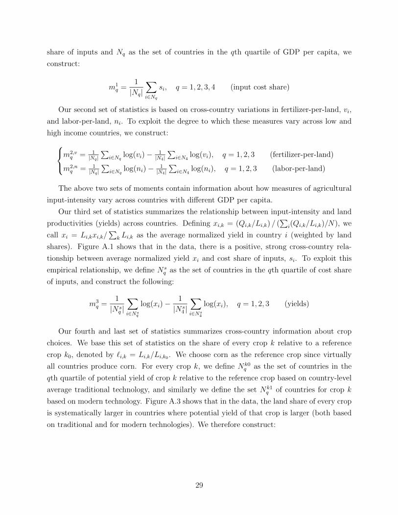
share of inputs and Nq as the set of countries in the qth quartile of GDP per capita, we

construct:

m1q =

1

|Nq|∑i∈Nq

si, q = 1, 2, 3, 4 (input cost share)

Our second set of statistics is based on cross-country variations in fertilizer-per-land, vi,

and labor-per-land, ni. To exploit the degree to which these measures vary across low and

high income countries, we construct:m2,vq = 1

|Nq |∑

i∈Nq log(vi)− 1|N4|∑

i∈N4log(vi), q = 1, 2, 3 (fertilizer-per-land)

m2,nq = 1

|Nq |∑

i∈Nq log(ni)− 1|N4|∑

i∈N4log(ni), q = 1, 2, 3 (labor-per-land)

The above two sets of moments contain information about how measures of agricultural

input-intensity vary across countries with different GDP per capita.

Our third set of statistics summarizes the relationship between input-intensity and land

productivities (yields) across countries. Defining xi,k = (Qi,k/Li,k) / (∑

i(Qi,k/Li,k)/N), we

call xi = Li,kxi,k/∑

k Li,k as the average normalized yield in country i (weighted by land

shares). Figure A.1 shows that in the data, there is a positive, strong cross-country rela-

tionship between average normalized yield xi and cost share of inputs, si. To exploit this

empirical relationship, we define N sq as the set of countries in the qth quartile of cost share

of inputs, and construct the following:

m3q =

1

|N sq |∑i∈Ns

q

log(xi)−1

|N s4 |∑i∈Ns

4

log(xi), q = 1, 2, 3 (yields)

Our fourth and last set of statistics summarizes cross-country information about crop

choices. We base this set of statistics on the share of every crop k relative to a reference

crop k0, denoted by ì,k = Li,k/Li,k0 . We choose corn as the reference crop since virtually

all countries produce corn. For every crop k, we define Nk0q as the set of countries in the

qth quartile of potential yield of crop k relative to the reference crop based on country-level

average traditional technology, and similarly we define the set Nk1q of countries for crop k

based on modern technology. Figure A.3 shows that in the data, the land share of every crop

is systematically larger in countries where potential yield of that crop is larger (both based

on traditional and for modern technologies). We therefore construct:

29

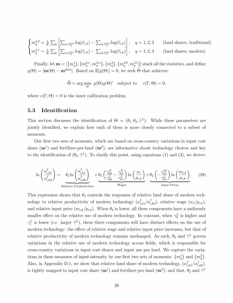
m4,0q = 1

K

∑k

[∑i∈Nk0

qlog(ì,k)−

∑i∈Nk0

4log(ì,k)

], q = 1, 2, 3 (land shares, traditional)

m4,1q = 1

K

∑k

[∑i∈Nk1

qlog(ì,k)−

∑i∈Nk1

4log(ì,k)

], q = 1, 2, 3 (land shares, modern)

Finally, let m = [m1q, m2,v

q ,m2,nq , m3

q, m4,0q ,m4,1

q ] stack all the statistics, and define

g(Θ) = [m(Θ)−mdata]. Based on E[g(Θ)] = 0, we seek Θ that achieves:

Θ = arg minΘ

g(Θ)g(Θ)′ subject to c(Γ; Θ) = 0,

where c(Γ; Θ) = 0 is the inner calibration problem.

5.3 Identification

This section discusses the identification of Θ = (θ1, θ2, γL). While these parameters are

jointly identified, we explain how each of them is more closely connected to a subset of

moments.

Our first two sets of moments, which are based on cross-country variations in input cost

share (m1) and fertilizer-per-land (m2), are informative about technology choices and key

to the identification of (θ2, γL). To clarify this point, using equations (1) and (3), we derive:

ln

(αfi,k1

αfi,k0

)= θ2 ln

(afi,k1

afi,k0

)︸︷︷︸

Relative Productivities

+ θ2

(γNk0

γLk0

−γNk1

γLk1

)ln

(wipi,k

)︸︷︷︸

Wages

+ θ2

(−γMk1

γLk1

)ln

(mi,k

pi,k

)︸︷︷︸

Input Prices

(29)

This expression shows that θ2 controls the responses of relative land share of modern tech-

nology to relative productivity of modern technology (afi,k1/afi,k0), relative wage (wi/pi,k),

and relative input price (mi,k/pi,k). When θ2 is lower, all these components have a uniformly

smaller effect on the relative use of modern technology. In contrast, when γL0 is higher and

γL1 is lower (i.e. larger γL), these three components will have distinct effects on the use of

modern technology: the effect of relative wage and relative input price increases, but that of

relative productivity of modern technology remains unchanged. As such, θ2 and γL govern

variations in the relative use of modern technology across fields, which is responsible for

cross-country variations in input cost shares and input use per land. We capture the varia-

tions in these measures of input-intensity by our first two sets of moments: m1q and m2

q.Also, in Appendix D.1, we show that relative land share of modern technology, (αfi,k1/α

fi,k0),

is tightly mapped to input cost share (m1) and fertilizer-per-land (m2); and that, θ2 and γL

30

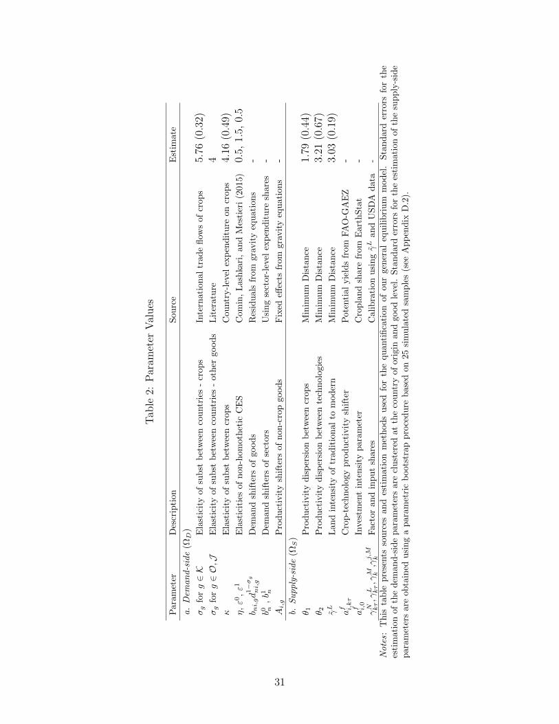
Tab

le2:

Par

amet

erV

alues

Par

amet

erD

escr

ipti

onSourc

eE

stim

ate

a.Dem

and-side

(ΩD

)

σg

forg∈K

Ela

stic

ity

ofsu

bst

bet

wee

nco

untr

ies

-cr

op

sIn

tern

ati

on

al

trade

flow

sof

crop

s5.

76(0

.32)

σg

forg∈O,J

Ela

stic

ity

ofsu

bst

bet

wee

nco

untr

ies

-oth

ergoods

Lit

eratu

re4

κE

last

icit

yof

subst

bet

wee

ncr

op

sC

ountr

y-l

evel

exp

endit

ure

on

crop

s4.

16(0

.49)

η,ε0

,ε1

Ela

stic

itie

sof

non

-hom

oth

etic

CE

SC

om

in,

Lash

kari

,an

dM

esti

eri

(2015)

0.5,

1.5,

0.5

b ni,gd1−σg

ni,g

Dem

and

shif

ters

of

goods

Res

idu

als

from

gra

vit

yeq

uati

on

s-

b0 n,b1 n

Dem

and

shif

ters

of

sect

ors

Usi

ng

sect

or-

leve

lex

pen

dit

ure

share

s-

Ai,g

Pro

duct

ivit

ysh

ifte

rsof

non-c

rop

good

sF

ixed

effec

tsfr

om

gra

vit

yeq

uati

ons

-b.

Supply-side

(ΩS

)

θ 1P

roduct

ivit

ydis

per

sion

bet

wee

ncr

ops

Min

imum

Dis

tance

1.79

(0.4

4)θ 2

Pro

duct

ivit

ydis

per

sion

bet

wee

nte

chnolo

gie

sM

inim

um

Dis

tance

3.21

(0.6

7)γL

Lan

din

tensi

tyof

trad

itio

nal

tom

oder

nM

inim

um

Dis

tance

3.03

(0.1

9)af i,kτ

Cro

p-t

ech

nol

ogy

pro

duct

ivit

ysh

ifte

rP

ote

nti

al

yie

lds

from

FA

O-G

AE

Z-

af i,0

Inves

tmen

tin

tensi

typ

ara

met

erC

rop

land

share

from

Eart

hSta

t-

γN kτ,γL kτ,γM k

,γj,M

kF

acto

ran

din

put

share

sC

alibra

tion

usi

ngγL

and

USD

Ad

ata

-

Notes:

Th

ista

ble

pre

sents

sourc

esan

des

tim

atio

nm

eth

ods

use

dfo

rth

equ

anti

fica

tion

of

our

gen

eral

equ

ilib

riu

mm

odel

.Sta

ndard

erro

rsfo

rth

ees

tim

atio

nof

the

dem

and-s

ide

par

amet

ers

are

clu

ster

edat

the

cou

ntr

yof

ori

gin

an

dgood

level

.S

tand

ard

erro

rsfo

rth

ees

tim

ati

on

of

the

sup

ply

-sid

epar

amet

ers

are

obta

ined

usi

ng

apar

amet

ric

boot

stra

ppro

cedu

rebase

don

25

sim

ula

ted

sam

ple

s(s

eeA

pp

endix

D.2

).

31

play a key role in this mapping.

Our third set of moments, m3, reflects the extent to which land productivities are larger in

countries where agricultural production is input-intensive. This relationship is particularly

informative about γL. To provide intuition, we note that conditional on the producers’

selections, the ratio of modern-to-traditional average land productivity in a field equals

γL ≡ γLk0/γLk1 (see Appendix D.1). So, differences in land productivities (yields) between

countries that tend to use traditional technologies more intensively and those that use modern

technologies more intensively are informative about γL.

Our fourth set of moments, m4, contains information about crop choices, which is key

to the identification of θ1. Invoking equation 3, variations in returns to crops, captured by

afi,kτ and hi,kτ , induce smaller variations in crop-level land shares when θ1 is lower. The

identification of θ1 exploits the relationship between variations in land shares of crops and

variations in potential yields, controlling for the model-implied variations in hi,kτ .

5.4 Estimation Results

5.4.1 Estimated Parameters

Table 2 summarizes our estimation results. On the demand side, we have estimated the

elasticity of substitution for crops across supplying countries, σk, at 5.76; and the elasticity

of substitution across crops, κ, at 4.16. On the supply side, our estimation sets θ1 = 1.79,

θ2 = 3.21, and γL = 3.03.

32

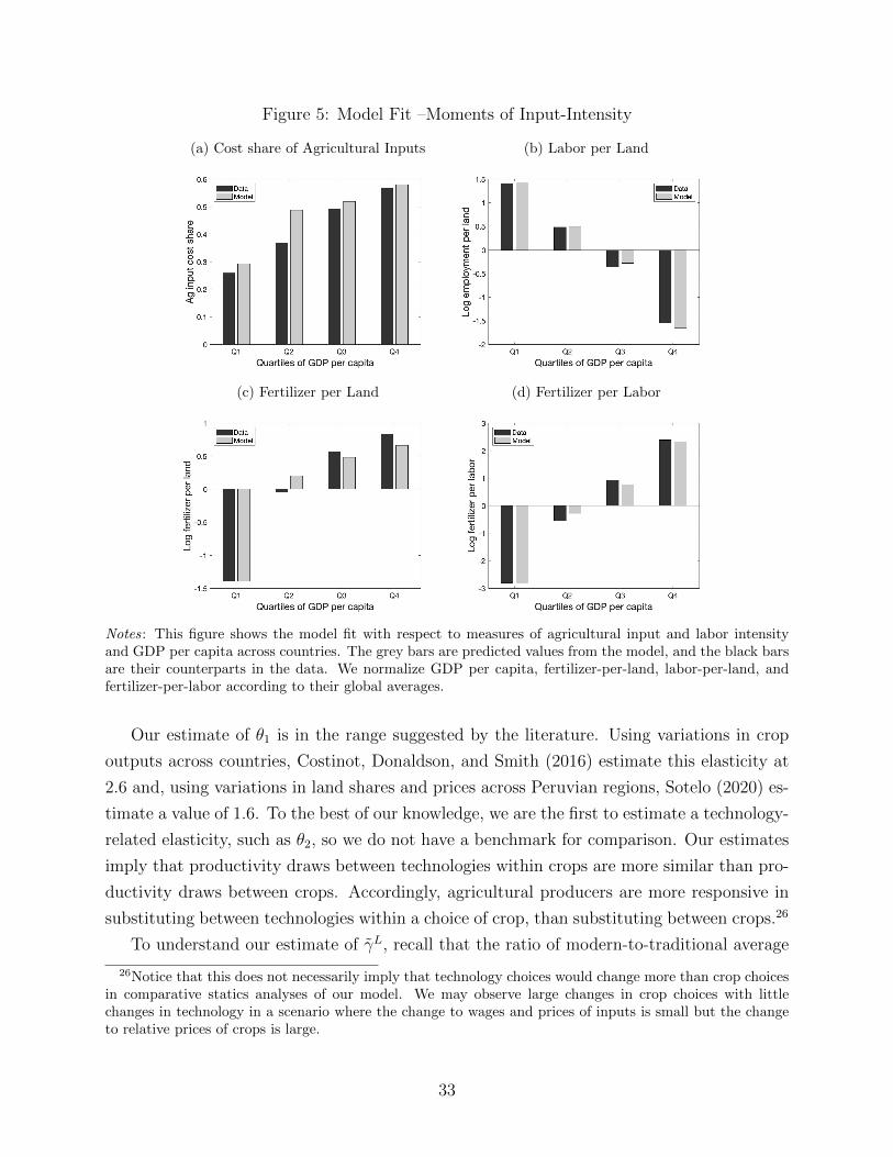
Figure 5: Model Fit –Moments of Input-Intensity

(a) Cost share of Agricultural Inputs (b) Labor per Land

(c) Fertilizer per Land (d) Fertilizer per Labor

Notes: This figure shows the model fit with respect to measures of agricultural input and labor intensityand GDP per capita across countries. The grey bars are predicted values from the model, and the black barsare their counterparts in the data. We normalize GDP per capita, fertilizer-per-land, labor-per-land, andfertilizer-per-labor according to their global averages.

Our estimate of θ1 is in the range suggested by the literature. Using variations in crop

outputs across countries, Costinot, Donaldson, and Smith (2016) estimate this elasticity at

2.6 and, using variations in land shares and prices across Peruvian regions, Sotelo (2020) es-

timate a value of 1.6. To the best of our knowledge, we are the first to estimate a technology-

related elasticity, such as θ2, so we do not have a benchmark for comparison. Our estimates

imply that productivity draws between technologies within crops are more similar than pro-

ductivity draws between crops. Accordingly, agricultural producers are more responsive in

substituting between technologies within a choice of crop, than substituting between crops.26

To understand our estimate of γL, recall that the ratio of modern-to-traditional average

26Notice that this does not necessarily imply that technology choices would change more than crop choicesin comparative statics analyses of our model. We may observe large changes in crop choices with littlechanges in technology in a scenario where the change to wages and prices of inputs is small but the changeto relative prices of crops is large.

33

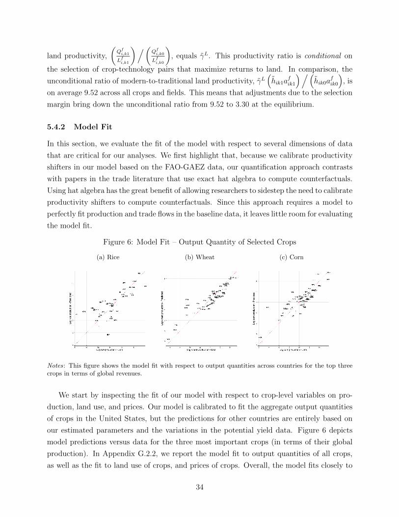
land productivity,

(Qfi,k1

Lfi,k1

)/(Qfi,k0

Lfi,k0

), equals γL. This productivity ratio is conditional on

the selection of crop-technology pairs that maximize returns to land. In comparison, the

unconditional ratio of modern-to-traditional land productivity, γL(hik1a

fik1

)/(hik0a

fik0

), is

on average 9.52 across all crops and fields. This means that adjustments due to the selection

margin bring down the unconditional ratio from 9.52 to 3.30 at the equilibrium.

5.4.2 Model Fit

In this section, we evaluate the fit of the model with respect to several dimensions of data

that are critical for our analyses. We first highlight that, because we calibrate productivity

shifters in our model based on the FAO-GAEZ data, our quantification approach contrasts

with papers in the trade literature that use exact hat algebra to compute counterfactuals.

Using hat algebra has the great benefit of allowing researchers to sidestep the need to calibrate

productivity shifters to compute counterfactuals. Since this approach requires a model to

perfectly fit production and trade flows in the baseline data, it leaves little room for evaluating

the model fit.

Figure 6: Model Fit – Output Quantity of Selected Crops

(a) Rice (b) Wheat (c) Corn

Notes: This figure shows the model fit with respect to output quantities across countries for the top threecrops in terms of global revenues.

We start by inspecting the fit of our model with respect to crop-level variables on pro-

duction, land use, and prices. Our model is calibrated to fit the aggregate output quantities

of crops in the United States, but the predictions for other countries are entirely based on

our estimated parameters and the variations in the potential yield data. Figure 6 depicts

model predictions versus data for the three most important crops (in terms of their global

production). In Appendix G.2.2, we report the model fit to output quantities of all crops,

as well as the fit to land use of crops, and prices of crops. Overall, the model fits closely to

34

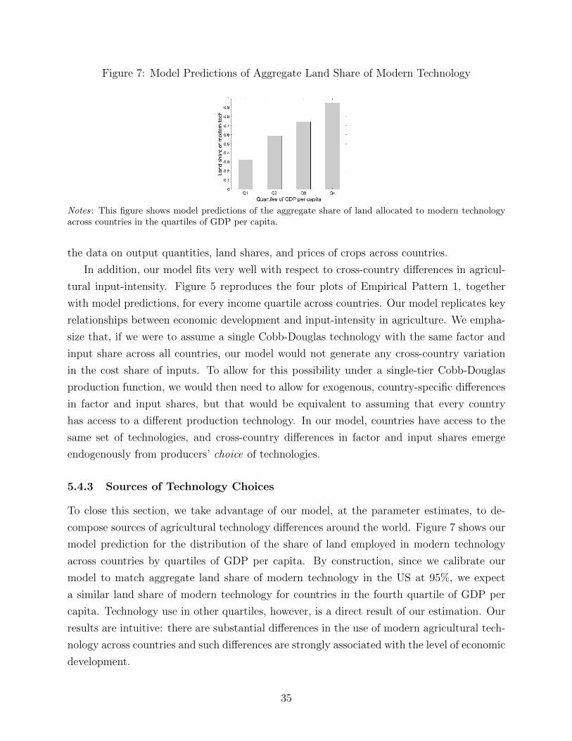
Figure 7: Model Predictions of Aggregate Land Share of Modern Technology

Notes: This figure shows model predictions of the aggregate share of land allocated to modern technologyacross countries in the quartiles of GDP per capita.

the data on output quantities, land shares, and prices of crops across countries.

In addition, our model fits very well with respect to cross-country differences in agricul-

tural input-intensity. Figure 5 reproduces the four plots of Empirical Pattern 1, together

with model predictions, for every income quartile across countries. Our model replicates key

relationships between economic development and input-intensity in agriculture. We empha-

size that, if we were to assume a single Cobb-Douglas technology with the same factor and

input share across all countries, our model would not generate any cross-country variation

in the cost share of inputs. To allow for this possibility under a single-tier Cobb-Douglas

production function, we would then need to allow for exogenous, country-specific differences

in factor and input shares, but that would be equivalent to assuming that every country

has access to a different production technology. In our model, countries have access to the

same set of technologies, and cross-country differences in factor and input shares emerge

endogenously from producers’ choice of technologies.

5.4.3 Sources of Technology Choices

To close this section, we take advantage of our model, at the parameter estimates, to de-

compose sources of agricultural technology differences around the world. Figure 7 shows our

model prediction for the distribution of the share of land employed in modern technology

across countries by quartiles of GDP per capita. By construction, since we calibrate our

model to match aggregate land share of modern technology in the US at 95%, we expect

a similar land share of modern technology for countries in the fourth quartile of GDP per

capita. Technology use in other quartiles, however, is a direct result of our estimation. Our

results are intuitive: there are substantial differences in the use of modern agricultural tech-

nology across countries and such differences are strongly associated with the level of economic

development.

35

To dissect variations that account for differences in technology choices around the world,

we make use of expression (29). Using the model-generated data at our estimated parameters,

we decompose sources of variations in technology choices using the Shapley decomposition.

The results are reported in Table 3.27 We first decompose the effect from exogenous pro-

ductivity premium (“local productivity premium”), and the combined effect of endogenous

wages and input prices (“local market condition”). Across all fields around the geography of

the world, variations in “local productivity premium” and “local market condition” account

respectively for 33% and 67% of the variations in technology use.28 We then zoom into the

components of local market conditions. Using equation (29),

ln

(αfi,k1

αfi,k0

)= θ2

(γNk0

γLk0

− γNk1

γLk1

)ln

(wipi,k

)+ θ2

(−γ

Mk1

γLk1

)ln

(mi,k

pi,k

), (30)

where ln αi,kτ = ln(αfi,kτ

)− θ2 ln

(afi,kτ

)is productivity-adjusted land share of technology τ .

Using equation (30), we find that variations in relative wage and relative input price account

for respectively 45% and 55% of variations in the productivity-adjusted land share of modern

to traditional technology.

Lastly, we zoom into the components of input price. We examine the contribution of

foreign trade in spatial variations in input prices. Invoking equation (11), the price index of

agricultural inputs for the production of crop k in country n can be expressed as:

logmn,k =

(∑j

γM,jk log pj,n

)︸︷︷︸

Domestic

+1

σ − 1

(∑j

γM,jk log λnn,j

)︸︷︷︸

Foreign

(31)

where pj,n ≡ pj,nb1/(1−σ)nn,j dnn,j is the domestic producer price adjusted by domestic demand

shifter. The first term captures the effect of domestic conditions of the market for inputs,

and the second term is an openness index that summarizes the effect from having access to

foreign inputs. Applying the Shapley decomposition to equation (31), we find that variations

in the openness index explains 29% of variations in input prices across countries.

This exercise shows the extent to which variations in each of the above-mentioned vari-

27The Shapley decomposition in our context determines the contribution of each right-hand-side variablein a regression by measuring the overall increase in R2 generated by the inclusion of each variable. SeeShorrocks (2013) for details about this decomposition method.

28Our results in this section complement findings from Adamopoulos and Restuccia (2018). Specifically,combining an accounting framework with the FAO-GAEZ data, and assuming that the same technology isemployed across countries, they find that differences in agro-ecological conditions account for a small shareof cross-country differences in agricultural land productivity. Here, our model indicates that differences inagro-ecological conditions explain one-third of spatial variations in the land share of modern to traditionaltechnology.

36

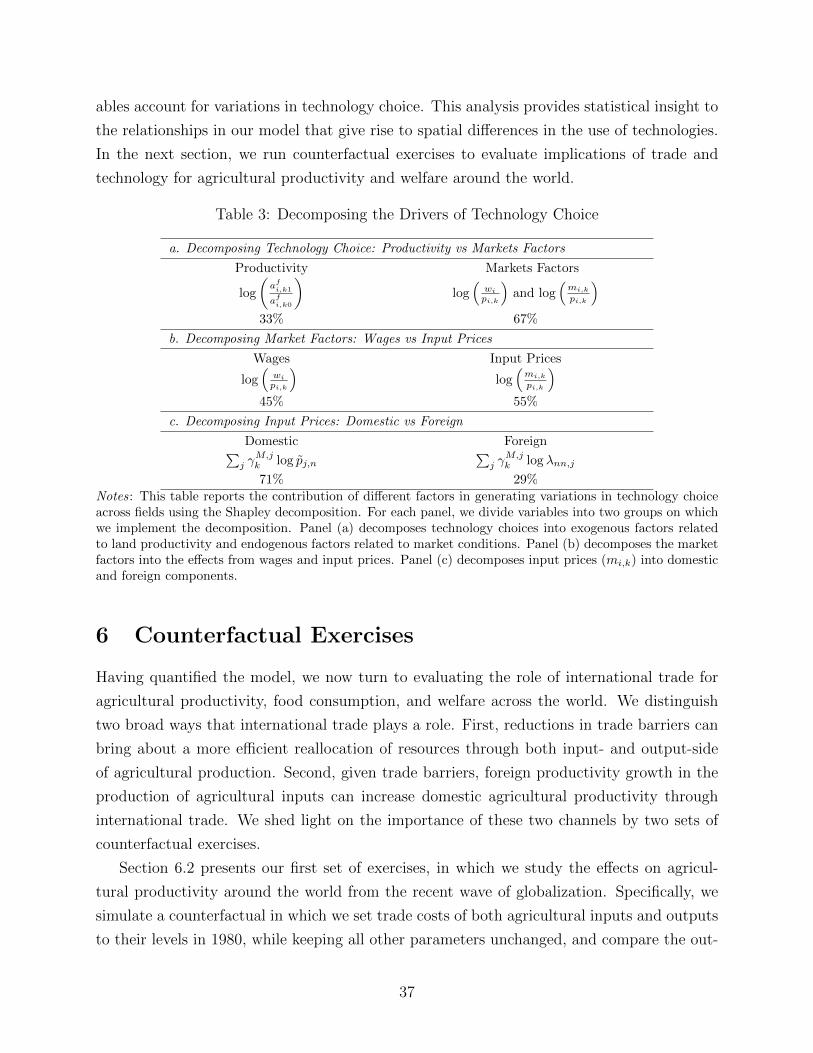
ables account for variations in technology choice. This analysis provides statistical insight to

the relationships in our model that give rise to spatial differences in the use of technologies.

In the next section, we run counterfactual exercises to evaluate implications of trade and

technology for agricultural productivity and welfare around the world.

Table 3: Decomposing the Drivers of Technology Choice

a. Decomposing Technology Choice: Productivity vs Markets Factors

Productivity Markets Factors

log

(afi,k1

afi,k0

)log(wipi,k

)and log

(mi,kpi,k

)33% 67%

b. Decomposing Market Factors: Wages vs Input Prices

Wages Input Prices

log(wipi,k

)log(mi,kpi,k

)45% 55%

c. Decomposing Input Prices: Domestic vs Foreign

Domestic Foreign∑j γ

M,jk log pj,n

∑j γ

M,jk log λnn,j

71% 29%

Notes: This table reports the contribution of different factors in generating variations in technology choiceacross fields using the Shapley decomposition. For each panel, we divide variables into two groups on whichwe implement the decomposition. Panel (a) decomposes technology choices into exogenous factors relatedto land productivity and endogenous factors related to market conditions. Panel (b) decomposes the marketfactors into the effects from wages and input prices. Panel (c) decomposes input prices (mi,k) into domesticand foreign components.

6 Counterfactual Exercises

Having quantified the model, we now turn to evaluating the role of international trade for

agricultural productivity, food consumption, and welfare across the world. We distinguish

two broad ways that international trade plays a role. First, reductions in trade barriers can

bring about a more efficient reallocation of resources through both input- and output-side

of agricultural production. Second, given trade barriers, foreign productivity growth in the

production of agricultural inputs can increase domestic agricultural productivity through

international trade. We shed light on the importance of these two channels by two sets of

counterfactual exercises.

Section 6.2 presents our first set of exercises, in which we study the effects on agricul-

tural productivity around the world from the recent wave of globalization. Specifically, we

simulate a counterfactual in which we set trade costs of both agricultural inputs and outputs

to their levels in 1980, while keeping all other parameters unchanged, and compare the out-

37

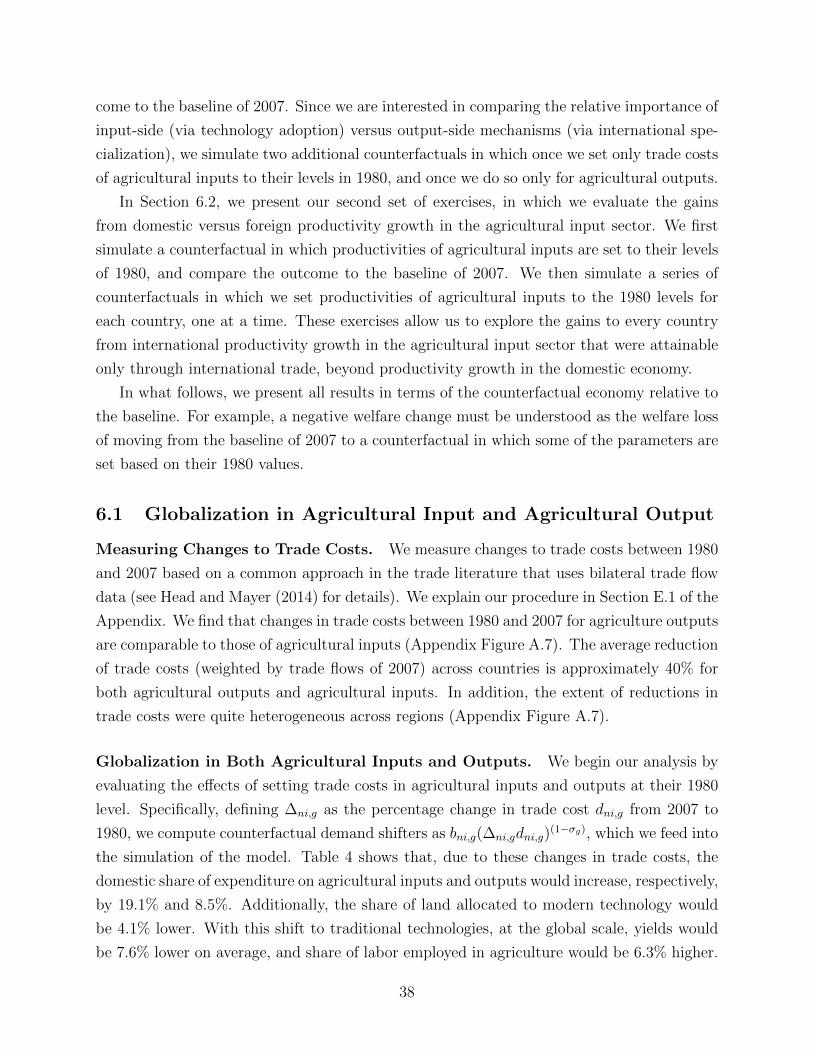
come to the baseline of 2007. Since we are interested in comparing the relative importance of

input-side (via technology adoption) versus output-side mechanisms (via international spe-

cialization), we simulate two additional counterfactuals in which once we set only trade costs

of agricultural inputs to their levels in 1980, and once we do so only for agricultural outputs.

In Section 6.2, we present our second set of exercises, in which we evaluate the gains

from domestic versus foreign productivity growth in the agricultural input sector. We first

simulate a counterfactual in which productivities of agricultural inputs are set to their levels

of 1980, and compare the outcome to the baseline of 2007. We then simulate a series of

counterfactuals in which we set productivities of agricultural inputs to the 1980 levels for

each country, one at a time. These exercises allow us to explore the gains to every country

from international productivity growth in the agricultural input sector that were attainable

only through international trade, beyond productivity growth in the domestic economy.

In what follows, we present all results in terms of the counterfactual economy relative to

the baseline. For example, a negative welfare change must be understood as the welfare loss

of moving from the baseline of 2007 to a counterfactual in which some of the parameters are

set based on their 1980 values.

6.1 Globalization in Agricultural Input and Agricultural Output

Measuring Changes to Trade Costs. We measure changes to trade costs between 1980

and 2007 based on a common approach in the trade literature that uses bilateral trade flow

data (see Head and Mayer (2014) for details). We explain our procedure in Section E.1 of the

Appendix. We find that changes in trade costs between 1980 and 2007 for agriculture outputs

are comparable to those of agricultural inputs (Appendix Figure A.7). The average reduction

of trade costs (weighted by trade flows of 2007) across countries is approximately 40% for

both agricultural outputs and agricultural inputs. In addition, the extent of reductions in

trade costs were quite heterogeneous across regions (Appendix Figure A.7).

Globalization in Both Agricultural Inputs and Outputs. We begin our analysis by

evaluating the effects of setting trade costs in agricultural inputs and outputs at their 1980

level. Specifically, defining ∆ni,g as the percentage change in trade cost dni,g from 2007 to

1980, we compute counterfactual demand shifters as bni,g(∆ni,gdni,g)(1−σg), which we feed into

the simulation of the model. Table 4 shows that, due to these changes in trade costs, the

domestic share of expenditure on agricultural inputs and outputs would increase, respectively,

by 19.1% and 8.5%. Additionally, the share of land allocated to modern technology would

be 4.1% lower. With this shift to traditional technologies, at the global scale, yields would

be 7.6% lower on average, and share of labor employed in agriculture would be 6.3% higher.

38

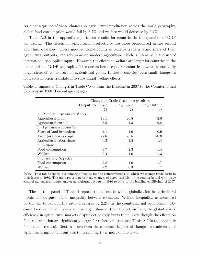
As a consequence of these changes in agricultural production across the world geography,

global food consumption would fall by 3.7% and welfare would decrease by 2.4%.

Table A.2 in the appendix reports our results for countries in the quartiles of GDP

per capita. The effects on agricultural productivity are more pronounced in the second

and third quartiles. These middle-income countries tend to trade a larger share of their

agricultural outputs, and rely more on modern agriculture which is intensive in the use of

internationally-supplied inputs. However, the effects on welfare are larger for countries in the

first quartile of GDP per capita. This occurs because poorer countries have a substantially

larger share of expenditure on agricultural goods. In these countries, even small changes in

food consumption translate into substantial welfare effects.

Table 4: Impact of Changes in Trade Costs from the Baseline in 2007 to the CounterfactualEconomy in 1980 (Percentage change)

Changes in Trade Costs in AgricultureOutput and Input Only Input Only Output

(1) (2) (3)

a. Domestic expenditure sharesAgricultural input 19.1 20.8 -2.8Agricultural output 8.5 -1.3 9.8

b. Agricultural productionShare of land in modern -4.1 -4.9 0.9Yield (avg across crops) -7.6 -6.5 -0.8Agricultural labor share 6.3 4.5 1.4

c. WelfareFood consumption -3.7 -2.3 -1.4Welfare -2.4 -1.0 -1.3

d. Inequality (Q4/Q1)Food consumption -2.8 -1.0 -1.7Welfare 2.2 0.3 1.7

Notes: This table reports a summary of results for the counterfactuals in which we change trade costs totheir levels in 1980. The table reports percentage changes of listed variable in the counterfactual with tradecosts of agricultural inputs and/or agricultural outputs in 1980 relative to the baseline equilibrium of 2007.

The bottom panel of Table 4 reports the extent to which globalization in agricultural

inputs and outputs affects inequality between countries. Welfare inequality, as measured

by the 4th to 1st quartile ratio, increases by 2.2% in the counterfactual equilibrium. Be-

cause low-income countries spend a larger share of their budget on food, the global loss of

efficiency in agricultural markets disproportionately hurts them, even though the effects on

food consumption are significantly larger for richer countries (see Table A.2 in the appendix

for detailed results). Next, we turn from the combined impact of changes in trade costs of

agricultural inputs and outputs to examining their individual effects.

39

Globalization Only in Agricultural Inputs & Only in Agricultural Outputs Col-

umn (2) and (3) of Table 4 present, separately, the impact of reductions in trade costs of only

agricultural inputs and only agricultural outputs. Overall, changes to yields, land share of

modern technology, and agricultural labor share are substantially larger in the case of trade

cost reductions in agricultural inputs (relative to agricultural outputs). It is also interesting

that in the counterfactual related to inputs, domestic expenditure share (DES) of outputs

slightly falls. This means that countries can produce more food for domestic consumption

by having a better access to internationally-supplied inputs. The opposite is also true. In

the counterfactual related to outputs, DES of agricultural inputs slightly decreases. This is

because, at the margin, countries can import crops in which they do not have a comparative

advantage instead of increasing domestic production of those crops using more inputs. As

such, the input-side and output-side mechanisms act slightly against each other.

The global welfare loss is 1.0% in the case of only inputs, and 1.3% in the case of only

outputs. In addition, the associated reduction in food consumption is 2.3% in the case of

inputs, compared to 1.4% in the case of outputs. We thus find that the effects of globalization

on welfare and food consumption via the input side of agriculture are as important as the

output side.

We also highlight that the effects from input side operate through distinct channels

(relative to output-side mechanisms). Panel (b) shows that yields are on average 6.5%

lower across crops in the input-only counterfactual. This sizable loss of yields is associated

with 20.8% increase in DES of agricultural inputs, 4.9% drop in the land share allocated

to modern technology, and 4.5% increase in agricultural labor share. These results echo

our theoretical analysis in Section 4.2. Due to larger trade barriers in the counterfactual,

agricultural inputs are relatively more expensive, hence agricultural producers rely more on

traditional technologies that have lower yields and use labor more intensively.

In addition, reductions in trade costs of agricultural inputs, compared to outputs, have

substantially different distributional implications. The welfare loss generated by raising trade

costs of agricultural outputs to their levels of 1980 is the largest for low-income countries—at

-2.5% for countries in the bottom quartile of GDP per capita—and the smallest for high-

income countries—at -0.8% for countries in the upper quartile of GDP per capita—. This

result is largely driven by the fact that countries have larger share of expenditure on food at

lower levels of income. The welfare loss generated by raising trade costs of agricultural inputs

to their levels of 1980, however, is the largest for the middle-income countries—at -1.3 and

-1.6% in the second and third quartiles of GDP per capita, respectively—. Two mechanisms

drive these results. First, increases in the trade costs of agricultural inputs have a larger

impact on the production costs of middle-income countries relative to low-income ones, since

40

low-income countries have a notably smaller share of their land under modern agriculture.

Second, in moving back to the counterfactual, middle-income countries compared to high-

income countries experience larger drops in the use of modern technologies: 5.7% for the

second quartile of the GDP per capita and 10.3 for the third quartile, while in high-income

countries, use of modern technology falls by only 0.4%. The resulting effect on welfare then

features an inverse-U shape along countries’ level of economic development.29 See Table A.2

for details.

6.2 Gains from Domestic and International Growth in Productiv-

ity of Agricultural Inputs

Measuring Changes to Productivity of Agricultural Inputs. We measure changes

to productivity of agricultural machinery and pesticides An,mach, An,pest, and production of

fertilizers Vn, for every country between 1980 and 2007. Our measures of productivity of

agricultural machinery and pesticides are based on the fixed effects recovered from gravity-

type equations for exports of manufacturing. Section E.2 in the Appendix describes this

procedure in details. For fertilizers, we calculate changes to production of fertilizers based

on data from FAO-STAT. The growth in productivity of agricultural inputs between 1980

and 2007 are large: productivity of agricultural machinery and pesticides, averaged across

countries, increased by approximately 126%; for fertilizers, global production increased by

55%.30

Impact of Productivity Changes in the Agricultural Input Sector. We consider

two sets of counterfactuals, which in total contain 1 + N counterfactual exercises. In the

first counterfactual, which we label as “shocks to all countries”, we re-calibrate An,mach,An,pest, VnNn=1 to their values in 1980 for all countries. In the next N counterfactuals, we

re-calibrate An,mach, An,pest, Vn to their values in 1980, for each country n, one at a time,

amounting to N independent outcomes. In each of these N counterfactuals, we focus on the

outcome of the country whose productivity parameters are re-calibrated. We refer to these

29We check the extent to which heterogeneous changes to trade costs are responsible for these distributionaloutcomes, and confirm that they do not alter the main takeaway. Specifically, we repeat our exercises for thecase where changes to trade costs are the same across countries and also between inputs and outputs (SeeTables A.3 and A.4 in the appendix). A main finding is that the welfare effect of globalization in agriculturaloutputs remains to be decreasing from the 4th to 1st quartile of GDP per capita, while the welfare effect ofglobalization in agricultural inputs remains to feature an inverse-U shape.

30The heterogeneity in productivity growth across regions is substantial, as shown in Figure A.8. Forexample, productivity of machinery and pesticides rose by 700% in East Asia and by 200% in the MiddleEast or Latin America. Production of fertilizers grew substantially across Asian countries while it slightlydeclined in Europe.

41

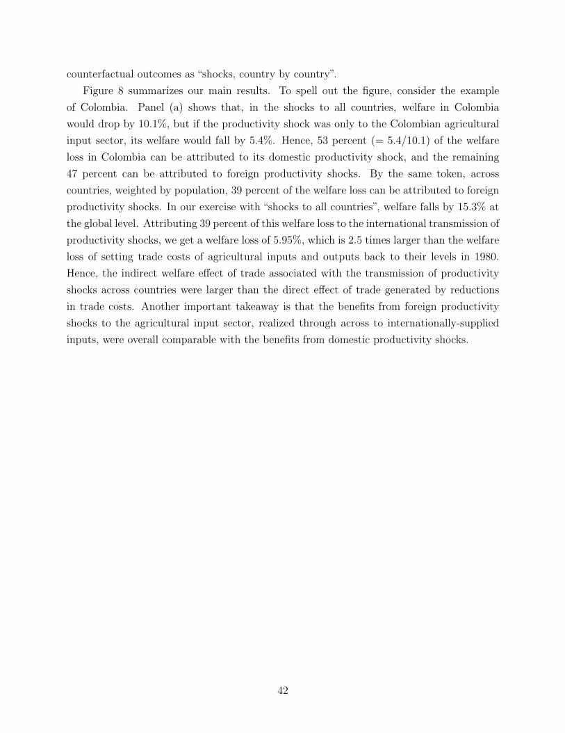
counterfactual outcomes as “shocks, country by country”.

Figure 8 summarizes our main results. To spell out the figure, consider the example

of Colombia. Panel (a) shows that, in the shocks to all countries, welfare in Colombia

would drop by 10.1%, but if the productivity shock was only to the Colombian agricultural

input sector, its welfare would fall by 5.4%. Hence, 53 percent (= 5.4/10.1) of the welfare

loss in Colombia can be attributed to its domestic productivity shock, and the remaining

47 percent can be attributed to foreign productivity shocks. By the same token, across

countries, weighted by population, 39 percent of the welfare loss can be attributed to foreign

productivity shocks. In our exercise with “shocks to all countries”, welfare falls by 15.3% at

the global level. Attributing 39 percent of this welfare loss to the international transmission of

productivity shocks, we get a welfare loss of 5.95%, which is 2.5 times larger than the welfare

loss of setting trade costs of agricultural inputs and outputs back to their levels in 1980.

Hence, the indirect welfare effect of trade associated with the transmission of productivity

shocks across countries were larger than the direct effect of trade generated by reductions

in trade costs. Another important takeaway is that the benefits from foreign productivity

shocks to the agricultural input sector, realized through across to internationally-supplied

inputs, were overall comparable with the benefits from domestic productivity shocks.

42

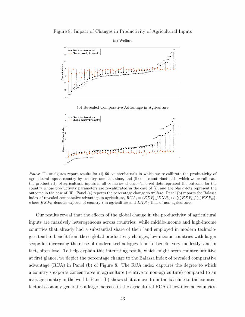
Figure 8: Impact of Changes in Productivity of Agricultural Inputs

(a) Welfare

(b) Revealed Comparative Advantage in Agriculture

Notes: These figures report results for (i) 66 counterfactuals in which we re-calibrate the productivity ofagricultural inputs country by country, one at a time, and (ii) one counterfactual in which we re-calibratethe productivity of agricultural inputs in all countries at once. The red dots represent the outcome for thecountry whose productivity parameters are re-calibrated in the case of (i), and the black dots represent theoutcome in the case of (ii). Panel (a) reports the percentage change to welfare. Panel (b) reports the Balassaindex of revealed comparative advantage in agriculture, RCAi = (EXPi1/EXPi0) / (

∑EXPi1/

∑EXPi0),

where EXPi1 denotes exports of country i in agriculture and EXPi0 that of non-agriculture.

Our results reveal that the effects of the global change in the productivity of agricultural

inputs are massively heterogeneous across countries: while middle-income and high-income

countries that already had a substantial share of their land employed in modern technolo-

gies tend to benefit from these global productivity changes, low-income countries with larger

scope for increasing their use of modern technologies tend to benefit very modestly, and in

fact, often lose. To help explain this interesting result, which might seem counter-intuitive

at first glance, we depict the percentage change to the Balassa index of revealed comparative

advantage (RCA) in Panel (b) of Figure 8. The RCA index captures the degree to which

a country’s exports concentrates in agriculture (relative to non-agriculture) compared to an

average country in the world. Panel (b) shows that a move from the baseline to the counter-

factual economy generates a large increase in the agricultural RCA of low-income countries,

43

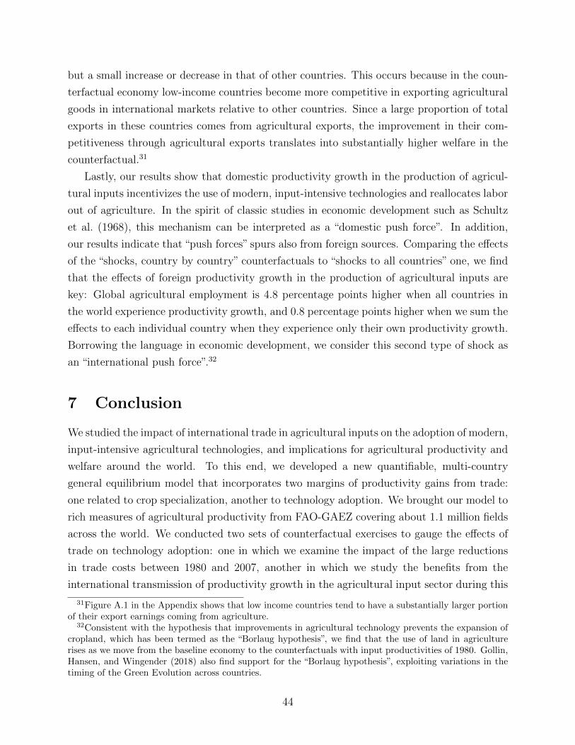
but a small increase or decrease in that of other countries. This occurs because in the coun-

terfactual economy low-income countries become more competitive in exporting agricultural

goods in international markets relative to other countries. Since a large proportion of total

exports in these countries comes from agricultural exports, the improvement in their com-

petitiveness through agricultural exports translates into substantially higher welfare in the

counterfactual.31

Lastly, our results show that domestic productivity growth in the production of agricul-

tural inputs incentivizes the use of modern, input-intensive technologies and reallocates labor

out of agriculture. In the spirit of classic studies in economic development such as Schultz

et al. (1968), this mechanism can be interpreted as a “domestic push force”. In addition,

our results indicate that “push forces” spurs also from foreign sources. Comparing the effects

of the “shocks, country by country” counterfactuals to “shocks to all countries” one, we find

that the effects of foreign productivity growth in the production of agricultural inputs are

key: Global agricultural employment is 4.8 percentage points higher when all countries in

the world experience productivity growth, and 0.8 percentage points higher when we sum the

effects to each individual country when they experience only their own productivity growth.

Borrowing the language in economic development, we consider this second type of shock as

an “international push force”.32

7 Conclusion

We studied the impact of international trade in agricultural inputs on the adoption of modern,

input-intensive agricultural technologies, and implications for agricultural productivity and

welfare around the world. To this end, we developed a new quantifiable, multi-country

general equilibrium model that incorporates two margins of productivity gains from trade:

one related to crop specialization, another to technology adoption. We brought our model to

rich measures of agricultural productivity from FAO-GAEZ covering about 1.1 million fields

across the world. We conducted two sets of counterfactual exercises to gauge the effects of

trade on technology adoption: one in which we examine the impact of the large reductions

in trade costs between 1980 and 2007, another in which we study the benefits from the

international transmission of productivity growth in the agricultural input sector during this

31Figure A.1 in the Appendix shows that low income countries tend to have a substantially larger portionof their export earnings coming from agriculture.

32Consistent with the hypothesis that improvements in agricultural technology prevents the expansion ofcropland, which has been termed as the “Borlaug hypothesis”, we find that the use of land in agriculturerises as we move from the baseline economy to the counterfactuals with input productivities of 1980. Gollin,Hansen, and Wingender (2018) also find support for the “Borlaug hypothesis”, exploiting variations in thetiming of the Green Evolution across countries.

44

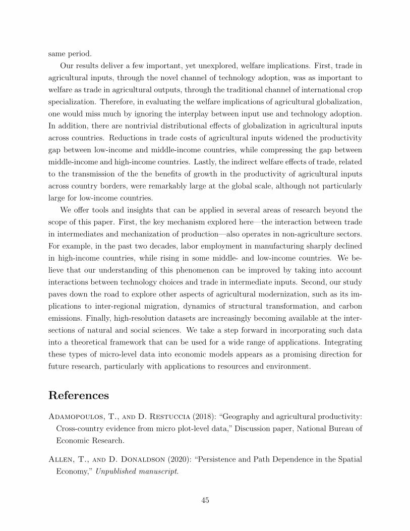
same period.

Our results deliver a few important, yet unexplored, welfare implications. First, trade in

agricultural inputs, through the novel channel of technology adoption, was as important to

welfare as trade in agricultural outputs, through the traditional channel of international crop

specialization. Therefore, in evaluating the welfare implications of agricultural globalization,

one would miss much by ignoring the interplay between input use and technology adoption.

In addition, there are nontrivial distributional effects of globalization in agricultural inputs

across countries. Reductions in trade costs of agricultural inputs widened the productivity

gap between low-income and middle-income countries, while compressing the gap between

middle-income and high-income countries. Lastly, the indirect welfare effects of trade, related

to the transmission of the the benefits of growth in the productivity of agricultural inputs

across country borders, were remarkably large at the global scale, although not particularly

large for low-income countries.

We offer tools and insights that can be applied in several areas of research beyond the

scope of this paper. First, the key mechanism explored here—the interaction between trade

in intermediates and mechanization of production—also operates in non-agriculture sectors.

For example, in the past two decades, labor employment in manufacturing sharply declined

in high-income countries, while rising in some middle- and low-income countries. We be-

lieve that our understanding of this phenomenon can be improved by taking into account

interactions between technology choices and trade in intermediate inputs. Second, our study

paves down the road to explore other aspects of agricultural modernization, such as its im-

plications to inter-regional migration, dynamics of structural transformation, and carbon

emissions. Finally, high-resolution datasets are increasingly becoming available at the inter-

sections of natural and social sciences. We take a step forward in incorporating such data

into a theoretical framework that can be used for a wide range of applications. Integrating

these types of micro-level data into economic models appears as a promising direction for

future research, particularly with applications to resources and environment.

References

Adamopoulos, T., and D. Restuccia (2018): “Geography and agricultural productivity:

Cross-country evidence from micro plot-level data,” Discussion paper, National Bureau of

Economic Research.

Allen, T., and D. Donaldson (2020): “Persistence and Path Dependence in the Spatial

Economy,” Unpublished manuscript.

45

Alvarez-Cuadrado, F., and M. Poschke (2011): “Structural change out of agriculture:

Labor push versus labor pull,” American Economic Journal: Macroeconomics, 3(3), 127–

58.

Antras, P., T. C. Fort, and F. Tintelnot (2017): “The margins of global sourcing:

Theory and evidence from us firms,” American Economic Review, 107(9), 2514–64.

Arkolakis, C., A. Costinot, and A. Rodriguez-Clare (2012): “New trade models,

same old gains,” American Economic Review, 102(1), 94–130.

Bergquist, L. F., B. Faber, T. Fally, M. Hoelzlein, E. Miguel, and

A. Rodriguez-Clare (2019): “Scaling Agricultural Policy Interventions: Theory and

Evidence from Uganda,” Working Paper.

Blaum, J., C. Lelarge, and M. Peters (2018): “The gains from input trade with

heterogeneous importers,” American Economic Journal: Macroeconomics, 10(4), 77–127.

Bustos, P. (2011): “Trade liberalization, exports, and technology upgrading: Evidence

on the impact of MERCOSUR on Argentinian firms,” American economic review, 101(1),

304–40.

Bustos, P., B. Caprettini, and J. Ponticelli (2016): “Agricultural productivity and

structural transformation: Evidence from Brazil,” American Economic Review, 106(6),

1320–65.

Caliendo, L., and F. Parro (2015): “Estimates of the trade and welfare effects of

NAFTA,” Review of Economic Studies, 82(1), 1–44.

Caselli, F. (2005): “Accounting for cross-country income differences,” Handbook of eco-

nomic growth, 1, 679–741.

Comin, D. A., D. Lashkari, and M. Mestieri (2015): “Structural change with long-run

income and price effects,” Discussion paper, National Bureau of Economic Research.

Conte, B., K. Desmet, D. K. Nagy, and E. Rossi-Hansberg (2020): “Local sectoral

specialization in a warming world,” .

Costinot, A., D. Donaldson, and C. Smith (2016): “Evolving comparative advantage

and the impact of climate change in agricultural markets: Evidence from 1.7 million fields

around the world,” Journal of Political Economy, 124(1), 205–248.

46

Costinot, A., and A. Rodrıguez-Clare (2014): “Trade theory with numbers: Quan-

tifying the consequences of globalization,” in Handbook of international economics, vol. 4,

pp. 197–261. Elsevier.

Donovan, K. (2017): “Agricultural risk, intermediate inputs, and cross-country productiv-

ity differences,” Working Paper.

Eaton, J., and S. Kortum (2002): “Technology, geography, and trade,” Econometrica,

70(5), 1741–1779.

Eaton, J., S. Kortum, and F. Kramarz (2011): “An anatomy of international trade:

Evidence from French firms,” Econometrica, 79(5), 1453–1498.

Fajgelbaum, P., and S. J. Redding (2019): “External integration, structural transforma-

tion and economic development: Evidence from argentina 1870-1914,” Discussion paper,

Working Paper.

Farrokhi, F. (2020): “Global sourcing in oil markets,”Journal of International Economics,

p. 103323.

Farrokhi, F., and A. Soderbery (2020): “Trade Elasticities in General Equilibrium,” .

Feenstra, R. C., R. E. Lipsey, H. Deng, A. C. Ma, and H. Mo (2005): “World

trade flows: 1962-2000,” Discussion paper, National Bureau of Economic Research.

Fieler, A. C., M. Eslava, and D. Y. Xu (2018): “Trade, quality upgrading, and input

linkages: Theory and evidence from colombia,” American Economic Review, 108(1), 109–

46.

Fuglie, K. (2012): “Productivity Growth and Technology Capital in the Global Agricul-

tural Economy,” Productivity growth in agriculture: An international perspective, p. 335.

Galle, S., A. Rodrıguez-Clare, and M. Yi (2017): “Slicing the pie: Quantifying

the aggregate and distributional effects of trade,” Discussion paper, National Bureau of

Economic Research.

Goldberg, P. K., A. K. Khandelwal, N. Pavcnik, and P. Topalova (2010): “Im-

ported intermediate inputs and domestic product growth: Evidence from India,” The

Quarterly journal of economics, 125(4), 1727–1767.

47

Gollin, D., C. W. Hansen, and A. Wingender (2018): “Two Blades of Grass: The

Impact of the Green Revolution,” Working Paper 24744, National Bureau of Economic

Research.

Gollin, D., S. L. Parente, and R. Rogerson (2007): “The food problem and the

evolution of international income levels,” Journal of Monetary Economics, 54(4), 1230–

1255.

Gouel, C., and D. Laborde (2018): “The crucial role of international trade in adaptation

to climate change,” Discussion paper, National Bureau of Economic Research.

Griliches, Z. (1958): “The demand for fertilizer: An economic interpretation of a technical

change,” Journal of Farm Economics, 40(3), 591–606.

Head, K., and T. Mayer (2014): “Gravity equations: Workhorse, toolkit, and cookbook,”

in Handbook of international economics, vol. 4, pp. 131–195. Elsevier.

Hertel, T. W. (2002): “Applied general equilibrium analysis of agricultural and resource

policies,” Handbook of agricultural economics, 2, 1373–1419.

Horowitz, J. L. (2001): “The bootstrap,” in Handbook of econometrics, vol. 5, pp. 3159–

3228. Elsevier.

Imbs, J., and I. Mejean (2015): “Elasticity optimism,” American Economic Journal:

Macroeconomics, 7(3), 43–83.

Inklaar, R., and M. P. Timmer (2008): “GGDC productivity level database: Interna-

tional comparisons of output, inputs and productivity at the industry level.,” Groningen

Growth and Development Centre Research Memorandum GD-104.

Johnson, W., and M. Fiszbein (2020): “Labor Push versus Comparative Advantage:

Agricultural Productivity, Openness, and Structural Change,” Working Paper.

Johnston, B. F., and J. W. Mellor (1961): “The role of agriculture in economic devel-

opment,” The American Economic Review, 51(4), 566–593.

Kucheryavyy, K., G. Lyn, and A. Rodrıguez-Clare (2016): “Grounded by gravity:

A well-behaved trade model with industry-level economies of scale,” Discussion paper,

National Bureau of Economic Research.

Lashkaripour, A., and V. Lugovskyy (2018): “Scale economies and the structure of

trade and industrial policy,” Working Paper.

48

Lind, N., and N. Ramondo (2018): “Trade with correlation,” Discussion paper, National

Bureau of Economic Research.

Matsuyama, K. (1992): “Agricultural productivity, comparative advantage, and economic

growth,” Journal of Economic Theory, 58(2), 317 – 334.

McArthur, J. W., and G. C. McCord (2017): “Fertilizing growth: Agricultural inputs

and their effects in economic development,” Journal of development economics, 127, 133–

152.

McFadden, D. (1981): “Econometric models of probabilistic choice,” Structural analysis of

discrete data with econometric applications, 198272.

Nagy, D. K. (2020): “Hinterlands, city formation and growth: Evidence from the US

westward expansion,” .

Nurkse, R. (1953): Problems of capital formation in underveloped countries. Oxford Uni-

versity Press.

Pellegrina, H. S. (2020): “Trade, Productivity and the Spatial Organization of Agricul-

ture: Evidence from Brazil ,” Working Paper.

Porteous, O. (2020): “Trade and agricultural technology adoption: Evidence from Africa,”

Journal of Development Economics, p. 102440.

Ramondo, N., and A. Rodrıguez-Clare (2013): “Trade, multinational production, and

the gains from openness,” Journal of Political Economy, 121(2), 273–322.

Restuccia, D., D. T. Yang, and X. Zhu (2008a): “Agriculture and aggregate produc-

tivity: A quantitative cross-country analysis,” Journal of Monetary Economics, 55(2), 234

– 250.

(2008b): “Agriculture and aggregate productivity: A quantitative cross-country

analysis,” Journal of monetary economics, 55(2), 234–250.

Rostow, W. W., and W. W. Rostow (1990): The stages of economic growth: A non-

communist manifesto. Cambridge university press.

Schultz, T. W., et al. (1968): “Economic growth and agriculture.,” Economic growth

and agriculture.

49

Shorrocks, A. F. (2013): “Decomposition procedures for distributional analysis: a unified

framework based on the Shapley value,” The Journal of Economic Inequality, 11(1), 99–

126.

Simonovska, I., and M. E. Waugh (2014): “The elasticity of trade: Estimates and

evidence,” Journal of international Economics, 92(1), 34–50.

Sotelo, S. (2020): “Domestic Trade Frictions and Agriculture,”Forthcoming in Journal of

Political Economy.

Taheripour, F., X. Zhao, M. Horridge, F. Farrokhi, and W. Tyner (2020): “Land

Use in Computable General Equilibrium Models,” Journal of Global Economic Analysis,

5(2), 63–109.

Teignier, M. (2018): “The role of trade in structural transformation,” Journal of Develop-

ment Economics, 130, 45–65.

Tombe, T. (2015): “The Missing Food Problem: Trade, Agriculture, and International

Productivity Differences,” American Economic Journal: Macroeconomics, 7(3), 226–258.

Yeaple, S. R. (2005): “A simple model of firm heterogeneity, international trade, and

wages,” Journal of international Economics, 65(1), 1–20.

50

Appendices for “Trade, Technology andAgriculture Productivity”

Farid Farrokhi and Heitor S. Pellegrina

A Data

This section describes in detail the datasets used in our paper. First, we present the data onpotential yields coming from FAO-GAEZ. Second, we describe the data on cropland from EarthStat.Third, we explain how we construct our data on trade and production, which combines informationfrom CEPII, OECD, STAN, FAO, and UNIDO. Lastly, we describe our construction of the dataon consumption shares and labor shares in agriculture, which uses data from the World Bank,Eurostat, and UN-ILO.

Potential Yields. The data on potential yields (also called ”maximum attainable yields”) comesfrom Global Agro-Ecological Zones (GAEZ) project, which is produced by the International Insti-tute for Applied System Analysis (IIASA) and the Food and Organization of the United Nations(FAO). The data is measured at the field level, which is often called in the literature as grid cellsor agro-ecological zones. Fields represent an area of 5 min by 5 min, which encompasses an areaof approximately 10 by 10 km. Among the different measures produced by FAO-GAEZ, we usefor our analysis data on agro-climatically attainable biomass by crop and specific land utilizationtypes (LUTs). The different types of land utilization corresponds to what we denote by differenttechnologies in our model. The estimation of the maximum attainable yield is based on a functionthat maps rich climate data into maximum attainable yields. The variables in the climate datainclude, among others, the dominant type of soil, altitude, slope, temperature, frost-free periodduring a year, and annual precipitation. In addition, the data is available for climates in differentreference periods. We pick the one that is based on the 1961-1990 period. The parameters ofthis function depend on each LUT and crop. Local socio-economic conditions do not enter as aninput in the estimation of maximum attainable yields. As such, variations in maximum attainableyields across fields reflect differences in agro-ecological conditions and not differences in the levelof economic development of a field. Indeed, we find little to no systematic variation between max-imum attainable yields and gdp per capita in our data once we control for a parsimonious set ofgeographic characteristics of a field.

In FAO-GAEZ, the land utilization types that define technologies in agricultural productionare divided into three groups. First, there is a low level of input use type, which corresponds to afarming system that is largely subsistence based. This dataset represents the maximum attainableyield if farmers use traditional cultivars and, importantly, no application of nutrients, no use ofchemicals and minimum conservation measures. Therefore, we denote this technology as traditionalin our analysis. Second, there is an intermediate level of input use type, which corresponds to afarming system that is partly market oriented. We do not directly use this type of technologybecause we do not have enough data to identify an additional set of parameters for factor- andinput-intensity in our model. Third, the high level of input use type, which corresponds to a modernfarming system. In this case, production is fully mechanized and uses optimum applications ofnutrients and chemical pest, disease and weed control.

Cropland. The data on the share of total cropland in every field comes from EarthStat. Thegrid cells defined by EarthStat are the same as the ones in FAO-GAEZ, a feature that greatlyfacilitates merging the data from these two sources. The project is a collaboration between theGlobal Landscapes Initiative at the University of Minnesota’s Institute on the Environment andthe Land Use and Global Environment Lab at the University of British Columbia. Among the

1

several datasets organized by EarthStat, we use information on the share of total cropland. Theconstruction of this dataset is based on two satellite imagery datasets circa 2000, Boston Univer-sity’s Moderate resolution Imaging Spectrometer (MODIS) and the Satellite Pour l’Observationde la Terre (SPOT) VEGETATION based on Global Land Cover 2000 (GC2000), and agriculturalinventory data. The agricultural inventory data is used to train a land cover classification thattakes the satellite imagery as an input. In particular, the inventory data set combines demographiccensuses, agricultural censuses and national level statistics from FAO-STAT.

Trade and Gross Output. Our data set on gross output and bilateral trade flows is con-structed based on the year of 2007, which serves as the baseline year throughout our paper, andinclude the following sectoral groups: non-agriculture, agriculture (not disaggregated by crops),agricultural inputs (disaggregated by fertilizers, machinery and pesticide), and crops. We nextexplain the procedures that we apply for the construction of the data for each of these sectoralgroups.

For the non-agriculture sector, we first bring bilateral trade flow data from BACI-CEPII. Wethen construct gross output using domestic expenditure shares (λii,0) as follows. We collect data ondomestic expenditure shares (λii,0) from the World-Input Output Database (WIOD), CEPII, andInput-Output tables from OECD. For the countries without direct data on domestic trade shares,we bring UNIDO data on gross output with sectoral disaggregation at the 2 digit level, whichallows us to separate agriculture from non-agriculture, and construct domestic expenditure shares(λii,0) using λii,0 = (Y data

i,0 −Xdatai,0 )/(Y data

i,0 −Xdatai,0 +Mdata

i,0 ), where Y datai,0 is the gross output, Xdata

i,0

is non-agriculture exports, and Mdatai,0 is non-agriculture imports. Finally, with our measures of

domestic trade shares, we construct implied gross output using Yi,0 = Xdatai,0 +Mdata

i,0 λii,0/(1−λii,0).For the agricultural sector as a whole, we follow a very similar procedure. We also use bilateraltrade flow data from BACI-CEPII, but we instead bring in gross-output data from STAN andFAO-STAT to construct λii,1 when domestic expenditure shares are not directly available.

For each category of agricultural input (fertilizers, pesticides and agricultural machinery), weconstruct our bilateral trade flow data using BACI-CEPII. Here, we emphasize that our categoriesof fertilizers, pesticides, and agricultural machinery are aggregation over HS-6 digit products thatare associated with any of these individual agricultural input categories. To identify these HS-codes, we closely follow the specifications used in FAO-STAT for the construction of trade data byagricultural inputs. We next turn to the construction of gross-output for each agricultural inputcategory.

To measure gross-output for agricultural machinery, we first bring data on domestic expenditureshares of agricultural machinery using UNIDO data disaggregated at the 4 digit level data, whichallows us to measure domestic expenditure share of agricultural machinery. When data was notavailable for a country, we used information on the domestic trade shares of general machinery. Ifdata on the domestic trade shares of general machinery were not available, we applied the followingprocedure. We construct the log of the hazard ratio of domestic trade share in manufacturing(log (λii,0/(1− λii,0))) , the log of the hazard ratio in domestic share of trade in non-agriculture(log(λii,0/ (1− λii,0)) and run a regression of the latter against the former adding the size of the logof the gross output in manufacturing. By targeting the log of the hazard ratios, we ensure that thepredicted values from our regressions are bounded between 0 and 1. The correlation between thepredicted trade shares and the actual ones is 0.82. Using the predicted values from this regression,we construct the domestic share of trade in agricultural machinery for the remaining countrieswithout data. For gross-output in pesticide, we apply the same procedure, but, for fertilizers, sincewe have data on quantities, we adopt a slightly different method.

To construct our data on gross-output for fertilizers, we take advantage of the availability ofdata on exports, production, consumption and imports of tonnes of fertilizer per nutrient fromFAO-STAT with our data on trade flows in values. The data on fertilizers from FAO-STAT comesdisaggregated according to three nutrients, i.e., nitrogen N , phosphate P and potassium K, whichform the basis of chemical fertilizers (NPK). For simplicity, we summed the weight of the totalamount of nutrients. Using the data from FAO-STAT, we construct the domestic share of consump-

2

tion by dividing imports in quantity by total consumption in quantity. Using this domestic share of

consumption (λQii,F ), we construct gross output in values using Yi,F = Xdatai,F +Mdata

i,F λQii,F /(1−λQii,F ).

Here, we rely on the assumption that domestic shares of consumption in quantity are equivalent todomestic share of consumption in values. This is the case when the price of imported fertilizers areon average the same as the price of fertilizers consumed from domestic source. This assumption isconsistent with the Eaton and Kortum (2002) framework, where the average price of goods in adestination coming from any source is the same. Given our information on quantities, we measuredthe unit value of fertilizers by dividing exports of a country to itself with data on the correspondingquantities.

To construct our gross output and bilateral flow data by crop, we bring in data from FAO-STAT. The bilateral trade flow data available in FAO-STAT is constructed based on COMTRADE(as is BACI-CEPII), which is the official international trade data coming from the United Nations.The main benefit of FAO-STAT is that it already comes organized by crop. We therefore have tomake minimal adjustments to crop names to ensure consistency between the trade and productiondata from FAO-STAT (in a few cases, a crop might be disaggregated in additional categories inthe trade data, for example, soy can be categorized as soy cake, soy powder and soy “in natura”).Since the data on revenues capture farm production, instead of revenues generated by processingindustries, we pick the codes associated with trade in less processed goods. For example, for oilpalm production we do not include data on bilateral trade flows in palm oil.

Lastly, for the non-agriculture and agriculture sector, we also constructed data on trade flowsand gross output for 1980, which we use in the paper to measures changes in trade costs andproductivity between 1980 and 2007. In this case, we adopt the same procedure as the one usedearlier, but we instead bring in bilateral trade flow data from Feenstra, Lipsey, Deng, Ma, and Mo(2005), which is also based on COMTRADE, given that data from BACI is not available for earlieryears.

Consumption Share and Labor Employment. To construct our data on consumptionshare in agricultural goods, we collect data from different sources. For developing countries, weuse data from the Global Consumption database organized by the World Bank to construct theconsumption shares in agricultural goods. For the United States, we use data from the consumerexpenditure survey. For Canada, we use data from household surveys available from Queen’sUniversity of Canada. For European countries, we bring data from Eurostat. To construct laboremployment, we use data from UN-ILO. When data from UN-ILO was not available, we infer theshare of workers in agriculture using data on the share of workers in rural areas from the WorldBank.

B Additional Empirical Patterns

In the main body of the article, we discussed key relationships between economic developmentand agricultural input intensity. This section discusses three additional empirical patterns thatmotivate our modeling approach and are important for understanding the effects of globalizationin our counterfactual analyses. The additional patterns are summarized in Figure A.1.

Panel (a) shows that the labor share in agriculture falls substantially with the level of eco-nomic development. This is consistent with high-income countries employing more input-intensivetechnologies for agricultural production.

Panel (b) documents that the share of final expenditure in agricultural goods falls with the levelof economic development. This is a feature of economic development that has long been discussedin the literature.We capture this relationship in out model using a non-homothetic CES.

Panel (c) shows that the share of exports of agricultural goods from total exports tends to belarger for countries with lower levels of income. For example, in Ethiopia almost 80% of the exportsare from the agricultural sector, whereas in Sweden this share is only 2.5%. This indicates thatagricultural sector is important not only because it accounts for an important share of the internal

3

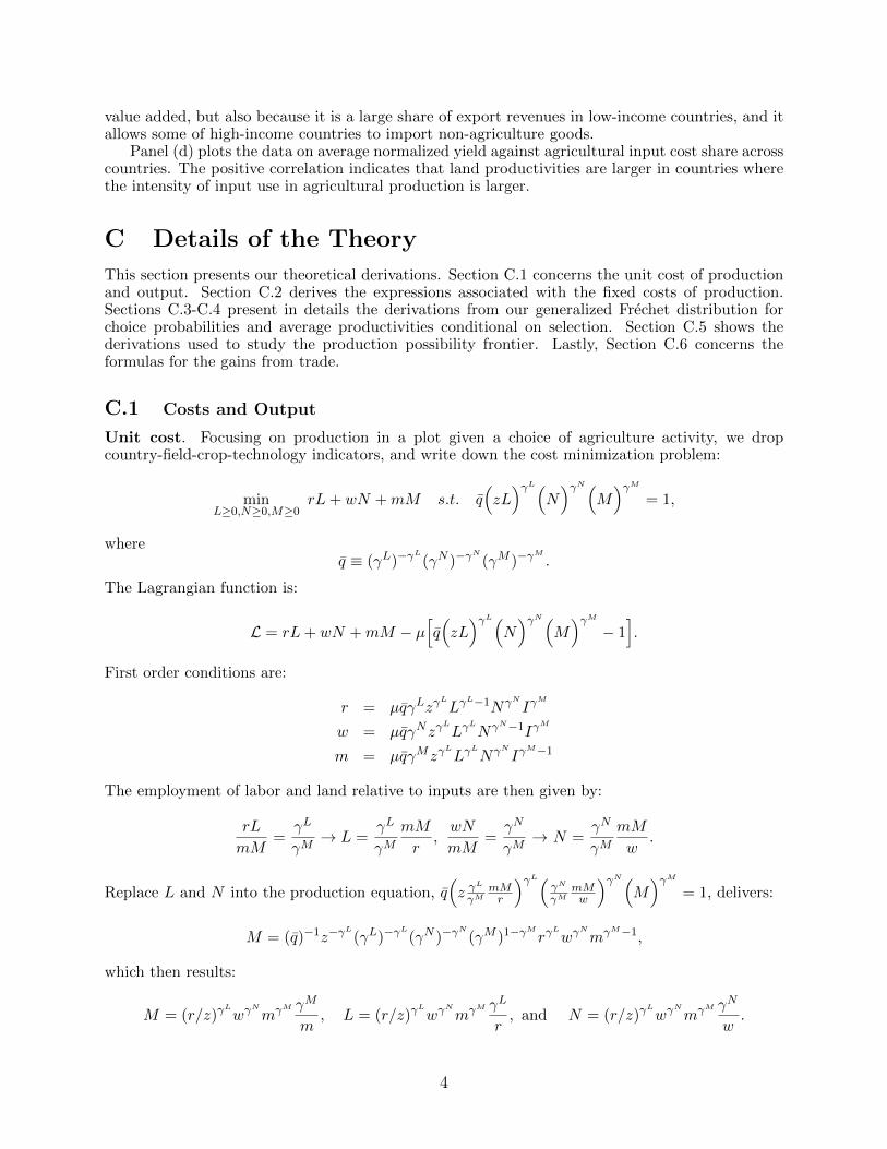
value added, but also because it is a large share of export revenues in low-income countries, and itallows some of high-income countries to import non-agriculture goods.

Panel (d) plots the data on average normalized yield against agricultural input cost share acrosscountries. The positive correlation indicates that land productivities are larger in countries wherethe intensity of input use in agricultural production is larger.

C Details of the Theory

This section presents our theoretical derivations. Section C.1 concerns the unit cost of productionand output. Section C.2 derives the expressions associated with the fixed costs of production.Sections C.3-C.4 present in details the derivations from our generalized Frechet distribution forchoice probabilities and average productivities conditional on selection. Section C.5 shows thederivations used to study the production possibility frontier. Lastly, Section C.6 concerns theformulas for the gains from trade.

C.1 Costs and Output

Unit cost. Focusing on production in a plot given a choice of agriculture activity, we dropcountry-field-crop-technology indicators, and write down the cost minimization problem:

minL≥0,N≥0,M≥0

rL+ wN +mM s.t. q(zL)γL(

N)γN(

M)γM

= 1,

whereq ≡ (γL)−γ

L

(γN )−γN

(γM )−γM

.

The Lagrangian function is:

L = rL+ wN +mM − µ[q(zL)γL(

N)γN(

M)γM− 1].

First order conditions are:

r = µqγLzγL

LγL−1NγN Iγ

M

w = µqγNzγL

LγL

NγN−1IγM

m = µqγMzγL

LγL

NγN IγM−1

The employment of labor and land relative to inputs are then given by:

rL

mM=

γL

γM→ L =

γL

γMmM

r,wN

mM=γN

γM→ N =

γN

γMmM

w.

Replace L and N into the production equation, q(z γ

L

γMmMr

)γL(γN

γMmMw

)γN(M)γM

= 1, delivers:

M = (q)−1z−γL

(γL)−γL

(γN )−γN

(γM )1−γM rγL

wγN

mγM−1,

which then results:

M = (r/z)γL

wγN

mγM γM

m, L = (r/z)γ

L

wγN

mγM γL

r, and N = (r/z)γ

L

wγN

mγM γN

w.

4

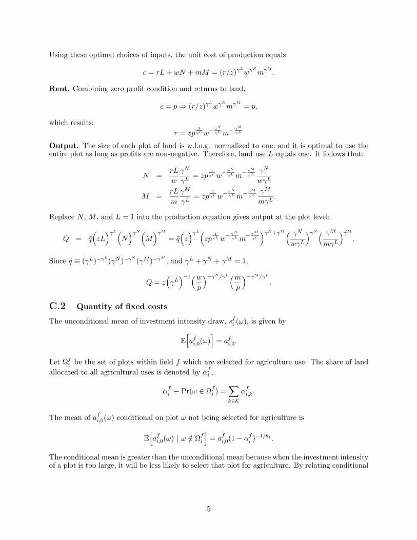
Using these optimal choices of inputs, the unit cost of production equals

c = rL+ wN +mM = (r/z)γL

wγN

mγM .

Rent. Combining zero profit condition and returns to land,

c = p⇒ (r/z)γL

wγN

mγM = p,

which results:

r = zp1

γLw− γ

N

γLm− γ

M

γL

Output. The size of each plot of land is w.l.o.g. normalized to one, and it is optimal to use theentire plot as long as profits are non-negative. Therefore, land use L equals one. It follows that:

N =rL

w

γN

γL= zp

1

γLw− γ

N

γLm− γ

M

γLγN

wγL

M =rL

m

γM

γL= zp

1

γLw− γ

N

γLm− γ

M

γLγM

mγL.

Replace N , M , and L = 1 into the production equation gives output at the plot level:

Q = q(zL)γL(

N)γN(

M)γM

= q(z)γL(

zp1

γLw− γ

N

γLm− γ

M

γL

)γN+γM( γNwγL

)γN( γMmγL

)γM.

Since q ≡ (γL)−γL

(γN )−γN

(γM )−γM

, and γL + γN + γM = 1,

Q = z(γL)−1(w

p

)−γN/γL(mp

)−γM/γL.

C.2 Quantity of fixed costs

The unconditional mean of investment intensity draw, sfi (ω), is given by

E[afi,0(ω)

]= afi,0.

Let Ωfi be the set of plots within field f which are selected for agriculture use. The share of land

allocated to all agricultural uses is denoted by αfi ,

αfi ≡ Pr(ω ∈ Ωfi ) =

∑k∈K

αfi,k.

The mean of afi,0(ω) conditional on plot ω not being selected for agriculture is

E[afi,0(ω) | ω /∈ Ωf

i

]= afi,0(1− αfi )−1/θ1 .

The conditional mean is greater than the unconditional mean because when the investment intensityof a plot is too large, it will be less likely to select that plot for agriculture. By relating conditional

5

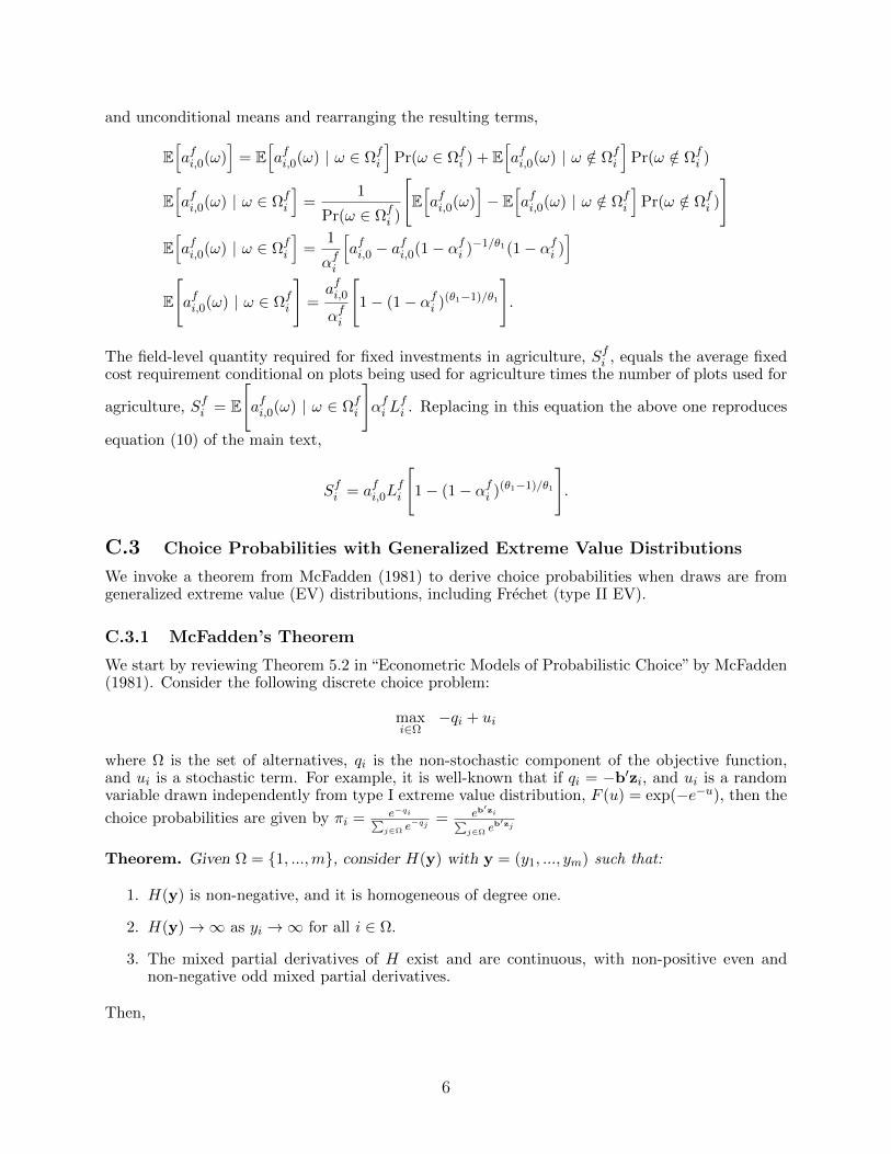
and unconditional means and rearranging the resulting terms,

E[afi,0(ω)

]= E

[afi,0(ω) | ω ∈ Ωf

i

]Pr(ω ∈ Ωf

i ) + E[afi,0(ω) | ω /∈ Ωf

i

]Pr(ω /∈ Ωf

i )

E[afi,0(ω) | ω ∈ Ωf

i

]=

1

Pr(ω ∈ Ωfi )

[E[afi,0(ω)

]− E

[afi,0(ω) | ω /∈ Ωf

i

]Pr(ω /∈ Ωf

i )

]E[afi,0(ω) | ω ∈ Ωf

i

]=

1

αfi

[afi,0 − a

fi,0(1− αfi )−1/θ1(1− αfi )

]E

[afi,0(ω) | ω ∈ Ωf

i

]=afi,0

αfi

[1− (1− αfi )(θ1−1)/θ1

].

The field-level quantity required for fixed investments in agriculture, Sfi , equals the average fixedcost requirement conditional on plots being used for agriculture times the number of plots used for

agriculture, Sfi = E

[afi,0(ω) | ω ∈ Ωf

i

]αfi L

fi . Replacing in this equation the above one reproduces

equation (10) of the main text,

Sfi = afi,0Lfi

[1− (1− αfi )(θ1−1)/θ1

].

C.3 Choice Probabilities with Generalized Extreme Value Distributions

We invoke a theorem from McFadden (1981) to derive choice probabilities when draws are fromgeneralized extreme value (EV) distributions, including Frechet (type II EV).

C.3.1 McFadden’s Theorem

We start by reviewing Theorem 5.2 in “Econometric Models of Probabilistic Choice” by McFadden(1981). Consider the following discrete choice problem:

maxi∈Ω

−qi + ui

where Ω is the set of alternatives, qi is the non-stochastic component of the objective function,and ui is a stochastic term. For example, it is well-known that if qi = −b′zi, and ui is a randomvariable drawn independently from type I extreme value distribution, F (u) = exp(−e−u), then the

choice probabilities are given by πi = e−qi∑j∈Ω e

−qj = eb′zi∑

j∈Ω eb′zj

Theorem. Given Ω = 1, ...,m, consider H(y) with y = (y1, ..., ym) such that:

1. H(y) is non-negative, and it is homogeneous of degree one.

2. H(y)→∞ as yi →∞ for all i ∈ Ω.

3. The mixed partial derivatives of H exist and are continuous, with non-positive even andnon-negative odd mixed partial derivatives.

Then,

6

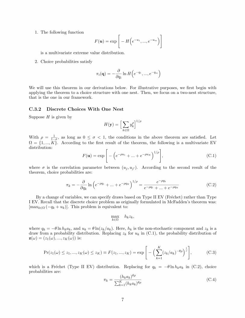
1. The following function

F (u) = exp

[−H

(e−u1 , ..., e−um

)]is a multivariate extreme value distribution.

2. Choice probabilities satisfy

πi(q) = − ∂

∂qilnH

(e−q1 , ..., e−qm

)We will use this theorem in our derivations below. For illustrative purposes, we first begin withapplying the theorem to a choice structure with one nest. Then, we focus on a two-nest structure,that is the one in our framework.

C.3.2 Discrete Choices With One Nest

Suppose H is given by

H(y) =[∑k∈Ω

yρk

]1/ρ

With ρ = 11−σ , as long as 0 ≤ σ < 1, the conditions in the above theorem are satisfied. Let

Ω = 1, ...,K. According to the first result of the theorem, the following is a multivariate EVdistribution:

F (u) = exp

[−(e−ρu1 + ...+ e−ρuK

)1/ρ], (C.1)

where σ is the correlation parameter between (uj , uj′). According to the second result of thetheorem, choice probabilities are:

πk = − ∂

∂qkln(e−ρq1 + ...+ e−ρqK

)1/ρ=

e−ρqk

e−ρq1 + ...+ e−ρqK(C.2)

By a change of variables, we can specify draws based on Type II EV (Frechet) rather than TypeI EV. Recall that the discrete choice problem as originally formulated in McFadden’s theorem was:[maxk∈Ω (−qk + uk)]. This problem is equivalent to:

maxk∈Ω

hkzk,

where qk = −θ lnhkak, and uk = θ ln(zk/ak). Here, hk is the non-stochastic component and zk is adraw from a probability distribution. Replacing zk for uk in (C.1), the probability distribution ofz(ω) = (z1(ω), ..., zK(ω)) is:

Pr(z1(ω) ≤ z1, ..., zK(ω) ≤ zK) ≡ F (z1, ..., zK) = exp

[−( K∑k=1

(zk/ak)−θρ) 1

ρ

], (C.3)

which is a Frechet (Type II EV) distribution. Replacing for qk = −θ lnhkak in (C.2), choiceprobabilities are:

πk =(hkak)

θρ∑Kk=1(hkak)θρ

(C.4)

7

The case of Eaton and Kortum (2002) with independent draws is a special case in which ρ = 1(or equivalently, σ = 0), and so, z1(ω), ..., zK(ω) are independent. The probability distributionsimplifies to

F (z1, ..., zK) = exp

[−( K∑k=1

(zk/ak)−θ)].

Thanks to independence of z1(ω), ..., zK(ω), the distribution of zk(ω) equals

Pr(zk(ω) ≤ zk) ≡ Fk(zk) = F (∞, ...∞, zK ,∞, ...∞) = exp[− (zk/ak)

−θ],

which is the distribution used in EK. In addition, setting ρ = 1 implies choice probabilities:

πk = (hkak)θ∑Kk=1(hkak)θ

.

C.3.3 Discrete Choices With Two Nests

The following function H satisfies the conditions in McFadden’s theorem,

H(y) =

K∑k=1

[ ∑τ∈Ωk

yρkτ

]1/ρ

Using the first result of the theorem, the following is a multivariate EV distribution

F (u) = exp

[−

K∑k=1

[ ∑τ∈Ωk

e−ρukτ]1/ρ

](C.5)

and, choice probabilities are as follows, based on the second result of the theorem,

πkτ = − ∂

∂qkτln

[K∑k=1

[ ∑τ∈Ωk

e−ρqkτ]1/ρ

]=

e−ρqkτ∑τ∈Ωk

e−ρqkτ×

[∑τ∈Ωk

e−ρqkτ]1/ρ

∑Kk=1

[∑τ∈Ωk

e−ρqkτ]1/ρ

(C.6)

The following changes of variables convert the formulation from EV type I to EV type IIdistribution: qkτ = −θ ln(akτhkτ ) and ukτ = θ ln(zkτ/akτ ). Replacing these in (C.5) and (C.8)delivers the distribution function of z = zkτkτ and choice probabilities:

F (z) = exp

[−

K∑k=1

[ ∑τ∈Ωk

(zkτ/akτ )−θρ]1/ρ

](C.7)

πkτ =(akτhkτ )θρ∑τ∈Ωk

(akτhkτ )θρ×

[∑τ∈Ωk

(akτhkτ )θρ]1/ρ

∑Kk=1

[∑τ∈Ωk

(akτhkτ )θρ]1/ρ

(C.8)

The connection from the above equation to the ones that describe land shares in the main text isimmediate. By setting θ2 = ρθ and θ1 = θ, the above readily delivers the four equations 2-3-4-5 ,

8

πkτ =(hkτakτ )θ2

Hθ2

k︸︷︷︸αkτ

Hθk∑

kHθk︸︷︷︸

αk

where Hk =[ T∑τ=1

(hkτakτ )θ2

] 1

θ2

C.4 Expected Value Conditional on Selection

In this section, we derive expected values of returns to land conditional on selections based ondiscrete choices. These derivations deliver average land productivities in our model conditional onchoices of crop-technology pairs. Again, for a clearer illustration, we first present the derivationfor the case with one nest, then we move to the two-nest distribution which is the case in ourframework.

C.4.1 One Nest

Reproducing equations (C.3) and (C.4),

Pr(z1(ω) ≤ z1, ..., zK(ω) ≤ zK) ≡ F (z1, ..., zK) = exp

[−( K∑k=1

(zk/ak)−θρ) 1

ρ

]

πk =(hkak)

θρ∑Kk=1(hkak)θρ

For notational simplicity, and w.l.o.g. we focus on the choice probability of the 1st alternative(k = 1). Let Ωj = ω : hjzj(ω) = maxk hkzk(ω), k = 1, ...,K. Define

F 1(z1, ..., zK) ≡ ∂

∂z1F (z1, ..., zK)

which equals:

F 1(z1, ..., zK) = θaθρ1 z−θρ−11

( K∑k=1

(zk/ak)−θρ) 1

ρ−1

exp

[−( K∑k=1

(zk/ak)−θρ) 1

ρ

]

9

The probability distribution of z1(ω) conditional on selecting the 1st alternative, ω ∈ Ω1,

F1(z) ≡ Pr(z1(ω) ≤ z | ω ∈ Ω1

)=

1

Pr(ω ∈ Ω1)Pr(z1(ω) ≤ z, h1z1(ω) ≥ hjzj(ω)

)=

1

π1Pr(z1(ω) ≤ z, zj(ω) ≤ h1

hjz1(ω)

)=

1

π1

∫ z

z1=0

∫ h1h2z1

z2=0

∫ h1hK

z1

zK=0f(z1, z2, ..., zK)dzK ...dz2dz1

=1

π1

∫ z

z1=0F 1(z1,

h1

h2z, ...,

h1

hKz1)dz1

=1

π1

∫ z

z1=0θaθρ1 z

−θρ−11

((z1

a1)−θρ +

K∑k=2

(h1z1

hkak)−θρ

) 1

ρ−1

exp

[−(

(z1

a1)−θρ +

K∑k=2

(h1z1

hkak)−θρ

) 1

ρ

]dz1

=1

π1

∫ z

z1=0θaθ1z

−θ−11

(1 +

K∑k=2

(h1a1

hkak)−θρ

) 1

ρ−1

exp

[− z−θaθ1

(1 +

K∑k=2

(h1a1

hkak)−θρ

) 1

ρ

]dz1

=1

π1

∫ z

z1=0θaθ1z

−θ−11

((h1a1)−θρ

K∑k=1

(hkak)θρ) 1

ρ−1

exp

[− z−θ1 aθ1

((h1a1)−θρ

K∑k=1

(hkak)θρ) 1

ρ

]dz1

=

∫ z

z1=0θaθ1z

−θ−11

( 1

π1

) 1

ρ

exp

[− z−θ1 aθ1

( 1

π1

) 1

ρ

]dz1

The last line is a Frechet distribution with c.d.f. exp(−Tz−θ1 ) with location parameter T = aθ1π−1/ρ1 .

It is straightforward to show that the expected value of this Frechet distribution equals Γ(1 −1/θ)T 1/θ. Putting together, the expected value of z1(ω) conditional on ω ∈ Ω1 equals

E(z1(ω)| ω ∈ Ω1

)= Γ(1− 1/θ)a1π

−1/θρ1

To make a closer connection to the notation we adopted in the main text, let θ2 ≡ θρ, and θ1 ≡ θ.Then,

Pr(z1(ω) ≤ z1, ..., zK(ω) ≤ zK) = exp

[−( K∑k=1

(zk/ak)−θ2

) θ1θ2

]And, the conditional expected value is given by

E(z1(ω)| ω ∈ Ω1

)= Γ(1− 1/θ1)a1π

−1/θ2

1

Note that, as in the main text, we could specify the distribution function by shifting the scale ofdraws according to some scalar φ > 0,

Pr(z1(ω) ≤ z1, ..., zK(ω) ≤ zK) = exp

[− φ

( K∑k=1

(zk/ak)−θ2

) θ1θ2

]

10

In this case, the conditional expected value equals: E(z1(ω)| ω ∈ Ω1

)= Γ(1−1/θ1)(φ)1/θ1a1π

−1/θ2

1

and the unconditional mean equals: E(z1(ω)

)= Γ(1 − 1/θ1)(φ)1/θ1a1. By choosing φ = [Γ(1 −

1/θ1)]−θ1 , we then ensure that E(z1(ω)| ω ∈ Ω1

)= a1π

−1/θ2

1 and E(z1(ω)

)= a1.

C.4.2 Two Nests

We now turn to the generalized Frechet distribution we have adopted in the text. For the sakeof a clear derivation, compared to the main text, we set the value of the outside option (i.e. theoption of not using a plot for agriculture) to zero. The alternatives in the upper nest are given by1, ...,K and in the lower nest within each k by 1, ..., T. Using equation (C.7) , we can expressthe generalized Frechet distribution as:

F (z) = exp

[− φ

K∑k=1

[ T∑τ=1


]

where z = [(z11, ..., z1T ), ..., (zk1, ..., zkT ), ...(zK1, ..., zKT )] with zkτ referring to the land productivity

draw of crop-technology pair kτ , and φ = [Γ(1− 1/θ)]−θ is a scalar. Using equation (C.8), thechoice probability of kτ equals:

πkτ =(hkτakτ )θρ

Hθρk

Hθk

Hθ1 + ...+Hθ

K

, where Hk =[(hk1ak1)θρ + ...+ (hkTakT )θρ

] 1

θρ

.

For notational simplicity and w.o.l.g, we focus on the choice of (k′, τ ′) = (1, 1). Defining F 11(z) ≡∂

∂z11F (z), we have:

F 11(z) = φθaθρ11z−θρ−111

( T∑τ=1

(z1τ/a1τ )−θρ) 1

ρ−1

exp

[− φ

K∑k=1

[ T∑τ=1


]

11

The probability distribution of z11(ω) conditional on ω ∈ Ω11 is then given by:

F11(z) ≡ Pr(z11(ω) ≤ z | ω ∈ Ω11

)=

1

Pr(ω ∈ Ω11)Pr(z11(ω) ≤ z, hkτzkτ (ω) ≤ h11z11(ω)

)=

1

π11Pr(z11(ω) ≤ z, zkτ (ω) ≤ h11

hkτz11(ω)

)=

1

π11

∫ z

z=0F 11(z

h11

h11,h11

h12z, ...,

h11

h1Tz, ...,

h11

hK1z, ...,

h11

hKTz)dz

=1

π11

∫ z

z=0φθaθρ11z

−θρ−1( T∑τ=1

(h11z

h1τa1τ)−θρ

) 1

ρ−1

exp

[− φ

K∑k=1

[ T∑τ=1

(h11z

hkτakτ)−θρ

]1/ρ]dz

=1

π11

∫ z

z=0φθaθ11z

−θ−1( T∑τ=1

(h11a11

h1τa1τ)−θρ

) 1

ρ−1

exp

[− φz−θaθ11

K∑k=1

[ T∑τ=1

(h11a11

hkτakτ)−θρ

]1/ρ]dz

=1

π11

∫ z

z=0φθaθ11z

−θ−1(

(h11a11)−θρT∑τ=1

(h1τa1τ )θρ) 1

ρ−1

× exp

[− φz−θaθ11

K∑k=1

[(h11a11)−θρ

T∑τ=1

(hkτakτ )θρ]1/ρ

]dz

Using Hk ≡(∑T

τ=1(hkτakτ )θρ)1/θρ

, and π11 = (h11a11)θρ

Hθρ1

Hθ1∑K

k=1 Hθk

, we simplify the last line into the

following:

F11(z) =

∫ z

z=0φθaθ11z

−θ−1(

(h11a11)−θK∑k=1

Hθk

)exp

[− φz−θaθ11(h11a11)−θ

K∑k=1

Hθk

].

Inspecting the above equation, it becomes evident that the distribution of z11(ω) conditional on

ω ∈ Ω11 is a Frechet with c.d.f F11(z) = exp(−Tz−θ) where the location parameter T equals

φaθ11

((h11a11)−θ

∑Kk=1H

θk

). It is straightforward to check that the expected value of a Frechet

distributed random variable with c.d.f. exp(−Tz−θ) equals Γ(1− 1/θ)T 1/θ. Hence,

E(z11(ω)|ω ∈ Ω11) = Γ(1− 1/θ)(φaθ11

((h11a11)−θ

∑Kk=1H

θk

))1/θ

Γ(1− 1/θ)(φ)1/θ

a11

((h11a11)θρ

Hθρ1

)−1/θρ (Hθ

1∑Kk=1 H

θk

)−1/θ

Notice that for the sake of tracking a clearer notation and with no loss of generality, we calculatedthe conditional expected value of crop-technology (k, τ) = (1, 1). Writing the expression for (k, τ),

noting that φ = [Γ(1− 1/θ)]−θ, and setting θ2 = θρ and θ1 = θ,

E(zkτ (ω)|ω ∈ Ωkτ ) = akτ

(hkτakτ )θ2

Hθ2

k︸︷︷︸αkτ

−1/θ2

Hθ1

k∑Kk=1H

θ1

k︸︷︷︸αk

−1/θ1

.

12

This derivation delivers the average land productivities conditional on the selection of a crop-technology pair as given by equation (6).

C.5 Derivations for Recasting the Micro-founded Structure to an Aggregate

Problem of PPF

In this section, we recast the land use problem onto crop supply through the lens of productionpossibility frontiers. We show that (i) the aggregate problem which describe below, reproducesequation (8), and (ii) the Lagrange multipliers of this problem reproduce returns to land. Recalling

that hi,kτ = pi,khi,kτand using an equivalent notation where Qfi,kτ = (γLkτ )−1hi,kτ Lfi,kτ , and Qfi,k =

Lfi,k, the problem of the agricultural producer in Section 4.1 can be written as:

maxQfi,kτk,τ , Qfi,kk

∑τ∈T

∑k∈K γ

Lkτpi,kQ

fi,kτ

subject to

[∑τ∈T

(Qfi,kτvfi,kτ

) θ2θ2−1

] θ2−1

θ2

≤ Qfi,k[∑k∈K(Qfi,k)

θ1θ1−1

] θ1−1

θ1

≤ Lfi

(C.9)

wherevfi,kτ = (γLkτ )−1hi,kτa

fi,kτ . (C.10)

The Lagrangian function associated with this maximization problem is:

L =∑τ

∑k

γLkτpi,kQfi,kτ − λ

fi,k

[∑τ

(Qfi,kτvfi,kτ

) θ2θ2−1

] θ2−1

θ2

− Qfi,k

− µfi

[∑k

(Qfi,k)θ1θ1−1

] θ1−1

θ1

− Lfi

Provided that the solution is interior, and quantities are all positive, the first order conditionsrequire that:

γLkτpi,k = µfi,k(vfi,kτ )

− θ2θ2−1 (Qfi,kτ )

1

θ2−1 (Qfi,k)− 1

θ2−1 (C.11)

µfi,k = µfi (Qfi,k)1

θ1−1 (Lfi )− 1

θ1−1 (C.12)

Using equation (C.11), and vfi,kτ = hi,kτafi,kτ (γLkτ )−1,

Qfi,kτ = (µfi,k)−(θ2−1)(γLkτ )−1(pi,k)

θ2−1(afi,kτ hi,kτ )θ2Qfi,k

or, equivalently,

Qfi,kτ

vfi,kτ= (µfi,k)

−(θ2−1)(pi,k)θ2−1(afi,kτ hi,kτ )θ2−1Qfi,k. (C.13)

Recall the definition of Hfi,k from equation (5),

Hfi,k =

[∑τ

(afi,kτpi,khi,kτ )θ2

] 1

θ2 .

13

Using equation (C.13),

[∑τ

(Qfi,kτvfi,kτ

) θ2θ2−1

] θ2−1

θ2

︸︷︷︸Qfi,k

= (µfi,k)−(θ2−1)Qfi,k(H

fi,k)

θ2−1,

which delivers the shadow price of crop k, µfi,k, that is precisely equal to Hfi,k,

µfi,k = Hfi,k. (C.14)

Let us now reproduce equation (C.12),

Qfi,k = (µfi,k)θ1−1(µfi )−(θ1−1)Lfi . (C.15)

which we use to derive the following relationship:[∑k

(Qfi,k)θ1θ1−1

] θ1−1

θ1

︸︷︷︸Lfi

= (µfi )−(θ1−1)Lfi

[∑k

(µfi,k)θ1

] θ1−1

θ1 .

Replacing µfi,k = Hfi,k from equation (C.14), we find the shadow price of total cropland, µfi ,

µfi =[∑

k

(Hfi,k)

θ1

] 1

θ1 . (C.16)

Plug µfi from (C.16) into (C.15),

Qfi,k = (µfi,k)θ1−1

[∑k

(µfi,k)θ1

]− θ1−1

θ1 Lfi =

[(Hf

i,k)θ1∑

k(Hfi,k)

θ1

] θ1−1

θ1

Lfi .

Replacing the above equation and equation (C.14) into equation (C.13), using vfi,kτ = (γLkτ )−1hi,kτafi,kτ ,

we have:

Qfi,kτ = (γLkτ )−1afi,kτ hi,kτ

[(afi,kτ hi,kτ )θ2

(Hfi,k)

θ2

] θ2−1

θ2

[(Hf

i,k)θ1∑

k(Hfi,k)

θ1

] θ1−1

θ1

Lfi .

This derivation reproduces equation (8) in the main text.

C.6 Derivations for the Gains from Trade

To highlight the main channels that drive the gains from trade, we simplify our model along twodimensions. First, suppose demand is a Cobb-Douglas combination between nonagriculture andagriculture that in turn consists of multiple crops:

Ci =(C0i

)β0i

(∏k

Cβi,ki,k

)β1i

,

14

where β0i and β1

i = 1− β0i are the share of expenditure on nonagriculture and agriculture, and βi,k

is the share of expenditure on crop k within agriculture. This means that compared to our mainmodel, β0

i , β1i , βi,k are exogenously fixed. Indirect utility is then given by:

Ci =Yi

(P 0i )β

0i (∏k P

βi,ki,k )β

1i

. (C.17)

Second, on the production side, we make the assumption that agriculture does not use labor.As such, let traditional technology use only land (γLk0 = 1), and modern technology use land and

intermediate inputs (γLk1 + γLM1 = 1). Value added generated by production of crop k in field f isthen given by

V fi,k = pi,kQ

fi,k0 + (1− γM1,k)pi,kQ

fi,k1.

Consider the equations that describe field-level crop quantities and relative land shares betweenthe two technologies,

Qfi,kτ = Lfi(γLkτ)−1

(mi,k

pi,k

)− γMk,τγLk,τ

afi,kτ

(αfi,k

) θ1−1

θ1

(αfi,kτ

) θ2−1

θ2 ,

αfi,k1

αfi,k0

=

(afi,k1

afi,k0

)(mi,k

pi,k

)− γMk,1γLk,1

θ2

.

Combining these two equations, we obtain relative output quantities between the two technologies:

Qfi,k1

Qfi,k0

=

(γLk1

γLk0

)−1(αfi,k1

αfi,k0

).

Replacing this into the expression for field-crop-specific value added, and noting that γLk0 = 1,

V fi,k = pi,kL

fi a

fi,k0(αfi,k)

θ1−1

θ1 (αfi,k0)−1

θ2 . (C.18)

By aggregation over fields, total value added from production of crop k equals:

Vi,k = pi,k∑f∈Fi

Lfi afi,k0(αfi,k)

θ1−1

θ1 (αfi,k0)−1

θ2 . (C.19)

We denote the value added share of nonagriculture by ρi,0 ≡ wiNiYi

and of crop k by ρi,k ≡ Vi,kYi

. In

addition, let the value added share of field f within crop k be ρfi,k ≡V fi,kVi,k

.

Consider a shock to trade costs that moves the baseline equilibrium to a new one. For anygeneric variable x, let x′ be its value in the new equilibrium, and x ≡ x′/x. Given the matrix of

trade cost changes, dni,k, from equation (11) that describes trade shares, we obtain:

λii,0 =

(wi

P 0i

)1−σ0

, λii,k =

(pi,k

Pi,k

)1−σk

. (C.20)

15

From equations (C.18)-(C.19), and noting that Vi,k = ρi,kYi,

pi,k = Vi,k

∑f Lfi a

fi,k0(αfi,kα

fi,k)

θ1−1

θ1 (αfi,k0αfi,k0)

−1

θ2∑f L

fi a

fi,k0(αfi,k)

θ1−1

θ1 (αfi,k0)−1

θ2

−1

= ρi,kYi

∑f

ρfi,k(αfi,k)

θ1−1

θ1 (αfi,k0)−1

θ2

−1

. (C.21)

Using equations (C.20)-(C.21) and noting that wi = ρi,0Yi, we can express the change to priceindexes of nonagriculture good and crops as:

P 0i = ρi,0Yi

(λii,0

) 1

σ0−1

, Pi,k = ρi,kYi

∑f

ρfi,k(αfi,k)

θ1−1

θ1 (αfi,k0)−1

θ2

−1 (λii,k

) 1

σk−1

. (C.22)

Replacing (C.22) into the hat-version of (C.17) reproduces equation (24) in the main text,

Ci =

(ρi,0

(λii,0

) 1

σ0−1

)−β0i ∏

k

(ρi,k

(λii,k

) 1

σk−1

)−β1i βi,k

∑f

ρfi,k(αfi,k)

θ1−1

θ1 (αfi,k0)−1

θ2

β1i βi,k

.

This reproduces equation (24) in the main text.

Now, suppose utility depends only on agriculture, i.e. β1i = 1, β0

i = 0, and there is only one crop,

i.e. αfi,k = βi,k = ρi,k = 1. Furthermore, suppose that in autarky, country i uses only traditionaltechnology for production, and has access to domestic agricultural variety for consumption. Giventhese assumptions, and dropping subscript k to collapse the model to one-sector economy, themagnitude of the gains from trade, calculated as the loss of welfare from moving the baselineeconomy to autarky (labeled as A), equals:

Gi ≡Ci − CAi

Ci= 1− (λii)

1

σ−1

∑f

ρfi (αfi,0)1

θ2

.Replacing αi,0 ≡

[∑f ρ

fi (αfi,0)

1

θ2

]θ2

, we can now reproduce equation (25) in the main text:

Gi = 1− (λii)1

σ−1 (αi,0)1

θ2 .

D Details about the Estimation

This section presents details about the estimation of the model. Section D.1 starts by presentingadditional discussion about the identification of the model. Section D.2 describes our bootstrapprocedure.

16

D.1 Additional Discussion about Identification

In the main body of the paper, we used the following relationship coming from our model to deriveexpression 29: (αi,k1

αi,k0

)=

[ai,k1

ai,k0×

(wi/pi,k)−γNk1/γ

Lk1(mi,k/pi,k)

−γMk1/γLk1

(wi/pi,k)−γNk0/γ

Lk0(mi,k/pi,k)−γ

Mk0/γ

Lk0

]θ2

.

We argued that (1) factor shares, γ-parameters, and θ2 control how prices and relative produc-tivities translate into relative land share of modern technology, (2) relative land share of moderntechnology is closely associated with the input cost share and input quantities per unit of land,which we target in our estimation. Using a pared-down version of our model, we now show howthese two sets of variables are tightly related to relative land share of modern technology. Inparticular, we assume that countries produce using a single crop and have a single field.

We start by deriving the expression for the input cost share. Let Cagi be total expenditure ininputs in agriculture, Ri be total revenues in agriculture, Ri0 and Ri1 be revenues, respectively,in traditional and modern sector in agriculture, and γM1 be the cost share of inputs. Therefore,CagiRagi

= γM1 Ri1Ri1+Ri0

,which can be written as:

CagiRagi

≡ γM11 +Ri0/Ri1

. (D.1)

We now show how Ri0/Ri1 relates to the inverse of relative land share of modern technology,αi0/αi1. To establish the link, we invoke the relative payments to land between the two technologies,riLi0riLi1

= γL0 Ri0γL1 Ri1

, which implies:

Ri0Ri1

=1

γLαi0αi1

(D.2)

where we defined γL ≡ γL0 /γL1 , which is a parameter we estimate in our model. The cost share of

inputs can thus be written as

CagiRagi

≡ γM1

1 +

(γLαi1αi0

)−1 . (D.3)

This expression shows how the relative share of land used in modern technology, αi1αi0, affects the

cost share of inputs, CagiRagi

, and how γL matters to that relationship In particular, controlling for

γM1 , when γL is larger, the same value of αi1αi0

translates to a larger cost share of inputs.We now discuss the relationship between input quantities per unit of land and relative land

share of modern technology. For concreteness, consider fertilizer-per-land, which is given by FiLi

=

riPi,F

γF,M1 γM1 Ri1(γL1 Ri1+γL0 Ri0)

. Combining this expression with equation (D.2),

FiLi

=riPi,F

γF,M1 γM1(γL1 + γL0

1

γLαi0αi1

) . (D.4)

Given that γL ≡ γL0 /γL1 , and αi0 = 1− αi1,we can rearrange the above expression to obtain:

FiLi

=riPi,F

γL

γL0γF,M1 γM1 αi1. (D.5)

17

Note that within the estimation of the model, we solve for equilibrium values of rents ri, pricesPi,F , and land shares αi1. The degree to which these variables influence Fi/Li is partly governedby γL.

Lastly, we discuss about yields (land productivities). While shifters of land productivity, afi,kτ ,are exogenous, land productivities in equilibrium —that is, conditional on the optimal selectionsof agricultural producers— are endogenous to local market conditions. Using equations (2) and(8), equilibrium yield of crop-technology pair (k, τ) in field f equals:

Qfi,kτ

Lfi,kτ= (γLkτ )−1hi,kτa

fi,kτ (αfi,k)

− 1

θ1 (αfi,kτ )− 1

θ2 (D.6)

First, we note that the land intensity parameter operates as a scalar of equilibrium yields. In-tuitively, a lower land intensity means higher intensity of non-land factors, hence a tendency fora higher land productivity. Using equation (3), this can be seen most clearly in the modern-to-traditional ratio of yields for the same crop in the same field,(

Qfi,k1

Lfi,k1

)/(Qfi,k0

Lfi,k0

)=

(γLk,1

γLk,0

)−1

= γL

When comparing yields across countries, local market conditions and productivity shifters in thosecountries would matter. However, controlling for them, a larger γL implies a larger gap betweenaverage equilibrium yields in countries that intensively use modern technologies relative to thosethat intensively use traditional technology.

D.2 Bootstrap

We compute standard errors of our structural estimation based on“parametric bootstrap”(Horowitz,2001). Our procedure works as follows. We assume that deviations between our model pre-dictions and data arise from measurement errors. For any country-level variable v, we specify:

yv,datai = yvi (Ω,X) + εvi where yv,datai is the log of our observation of variable v for country i, yviis its counterpart predicted by the model at the vector of parameters Ω and data X, and εvi is anerror term. By our specification, εvi is distributed according to a normal distribution N(0,Λv), andit is independent between countries and variables.

For our indirect inference, we construct aggregate statistics mdata from data points ydata ≡yv,datai . In the estimation, we minimize the distance between statistics m(Ω,X) predicted by the

model and their counterparts in the data, mdata. In particular, country-level variables which we useto construct our statistics are: v = agricultural expenditure on intermediate inputs, agriculturalgross output, quantity of fertilizer use, agricultural labor employment, crop-specific land use.Using our estimates of the model at Ω, we compute predicted residuals: εvi = ydata,vi − yv. Using

ε ≡ εvi , we estimate the empirical counterpart of the variance, Λv. We then draw the error

terms, εv,li from N(0, Λv), where l = 1, ..., L indexes the l-th set of simulated data. Using this

procedure, we create a new set of model-generated data points: yv,li = yvi + εv,li . We call the l-th

set of simulated data as yl ≡ yv,li . For each simulated data set yl, we repeat our estimation

algorithm in its entirety, and obtain estimates of Ωl. Lastly, we calculate confidence intervals and

standard errors based on the distribution of ΩlLl=1.

18

E Details about the Counterfactual Simulations

This section describes how we measure changes in trade cost and productivity between 1980 and2007 across countries, which we use in our counterfactual simulations. Section E.1 first describeshow we measure changes in trade cost. Section E.2 then explains how we measure changes inproductivity.

E.1 Measuring changes in trade costs

The method that we apply to measure changes in trade cost follow closely the literature usinggravity trade models (see Head and Mayer (2014) for a detailed description of such methods). Inparticular, we assume that the trade costs that compose the residuals introduced in Section 5.1(bni,gd

1−σkni,g ) include a symmetric trade cost component, which we denote by dni,g. As such, one

can easily use the demand equations from our model to write:

log

(Xin,g

Xii,g× Xin,g

Xnn,g

)= 2(1− σg) log(dni,g)︸︷︷︸

δin,g

+εin,g

where εin,g = log(bni,gbin,g/bii,gbni,g). Since the values of δin,g are relative to a baseline group, weadopt the common approach in the literature and assume that dni,g = 1, which sets δii,g = 0. Usingthis assumption, we recover the fixed effects δin,g, we then use our values of σg to recover dni,g.

Notice that, to recover the trade costs using the expression above, we need to measure thesales of a country to itself Xii,g, which requires data on gross output. Unfortunately, data forgross output disaggregated by category of agricultural input or by crop is not available for 1980.To circumvent this limitation, we estimate trade costs using data for more aggregate sectors,agriculture and non-agriculture and, in our counterfactuals, we apply the changes in trade costsin non-agriculture to simulate the effects of globalization for agricultural inputs. To validate thisapproach, we use data for 2007 to compare the trade costs that we obtain for the aggregate ofagricultural inputs (pesticides, machinery and fertilizers) and for the aggregate of non-agriculture.The correlation between these two measures of trade costs is high (ρ = 0.75), indicating that tradecosts in non-agriculture serves as a good proxy for trade costs in agricultural inputs.

Figure A.7 shows percentage changes to trade costs between 1980 and 2007 for agriculturaloutputs and inputs, aggregated by regions. We find an average reduction of trade costs of 39% foroutputs and by 41% for inputs. The fall in trade costs of agricultural inputs is typically larger thanthat of agricultural output. For both cases changes to trade costs are substantially heterogeneousacross regions.

E.2 Measuring changes in productivity

In Section 5.1 in the main body of the paper, we estimated productivities using the gravity structureof our model. In particular, controlling for value added per worker, we recovered productivitiesfrom the origin fixed effects of regressions in which we use consumption shares as the dependentvariable. We use the same procedure to measure relative productivities for agricultural machineryand pesticides in 1980. Similar to the limitation that we have in the case of trade cost, the lack ofdata on gross output for agricultural machinery and pesticide in 1980 prevents us from estimatingrelative productivities in 1980. We therefore use data on changes in productivity in non-agriculturebetween 1980 and 2007 as a proxy for the changes in productivity in machinery and pesticide. Thecorrelation between productivity in non-agriculture in 2007 and the productivity of agriculturalinputs as a whole is 0.98, which indicates that productivity in non-agriculture serves as a goodproxy for productivity in agricultural inputs. Finally, to pin down the level of productivities sothat we can compare 1980 with 2007, we bring in data from GGDC Productivity Level Databaseon the productivity of the US in tradeable goods (Inklaar and Timmer, 2008).

19

F Numerical Algorithms

This Section describes in detail the algorithms that we use to simulate and calibrate our model.Section F.1 starts by presenting the algorithm which we use to simulate the model. Section F.2presents the calibration algorithm (i.e. inner problem) which we use in the structural estimationof our model.

F.1 Simulation of Model Equilibrium

Our solution algorithm takes endowments E ≡ Lfn, Nn, Vn, supply parameters ΩS ≡ θ1, θ2, γLkτ ,

γMkτ , γNkτ , γ

j,Mk , afn,0, a

fn,kτ, and demand parameters ΩD ≡ ε0, ε1, η, κ, σg, b

sn, bn,k, bni,g, dni,g, An,g

as given, and solves for the vector of equilibrium prices.

1. Guess the vector wages wii∈N , crop prices pi,ki∈N ,k∈K, and fertilizer prices pi,fertn∈N .

2. Calculate prices of nonagriculture, pesticides, agricultural machinery according to pi,0 =wi/Ai,0, pi,pest = wi/Ai,pest and pi,mach = wi/Ai,mach. (All these prices, pi,g, are at thelocation of supply.)

3. For every good g (every of the crops, nonagriculture, fertilizer, pesticide, and agriculturalmachinery), calculate the price index at the location of consumption, Pn,g, according toequation (15), and expenditure (trade) share of every destination country n on every origincountry i, λni,g, according to equation (11).

4. (a) Compute the price index of agriculture, P 1n , according to equation (15), and expenditure

share on crops, βn,k, according to (12). (b) Price index of sector-level nonagriculture bundleis P 0

n = Pn,0. (c) Compute the aggregate price of intermediate inputs, mn,k, according to

mn,k =∏j∈J (Pn,j)

γj,Mk .

5. (a) Calculate hn,kτ and hn,kτ according to (1). (b) Calculate Hfn,k according to (5).

6. Calculate land shares of crops, αfn,k, and of technologies within every crop, αfn,kτ , based on

equations (3)-(4).

7. (a) Compute production quantities at the level of field, Qfn,kτ , based on (8), and at the level

of country, Qn,k, based on (9). (b) Compute aggregate quantity of investment, Sn, accordingto (10).

8. Calculate labor employment in agriculture, N1n, based on (20). Labor employment elsewhere

is Nn,rest = Nn −N1n.

9. Calculate revenues generated from every of the crops, fertilizers, and the“rest”of the economy(pesticides, agricultural machinery, and nonagriculture), that are:

Yn,k = pn,kQn,k, Yn,fert = pn,fertVn, Yn,rest = wnNn,rest

10. Calculate total expenditure in every country n, En, according to equation (21).

11. Compute aggregate final consumption, Cn, and its corresponding price index, Pn, accordingto:

(a) Guess Cn.

20

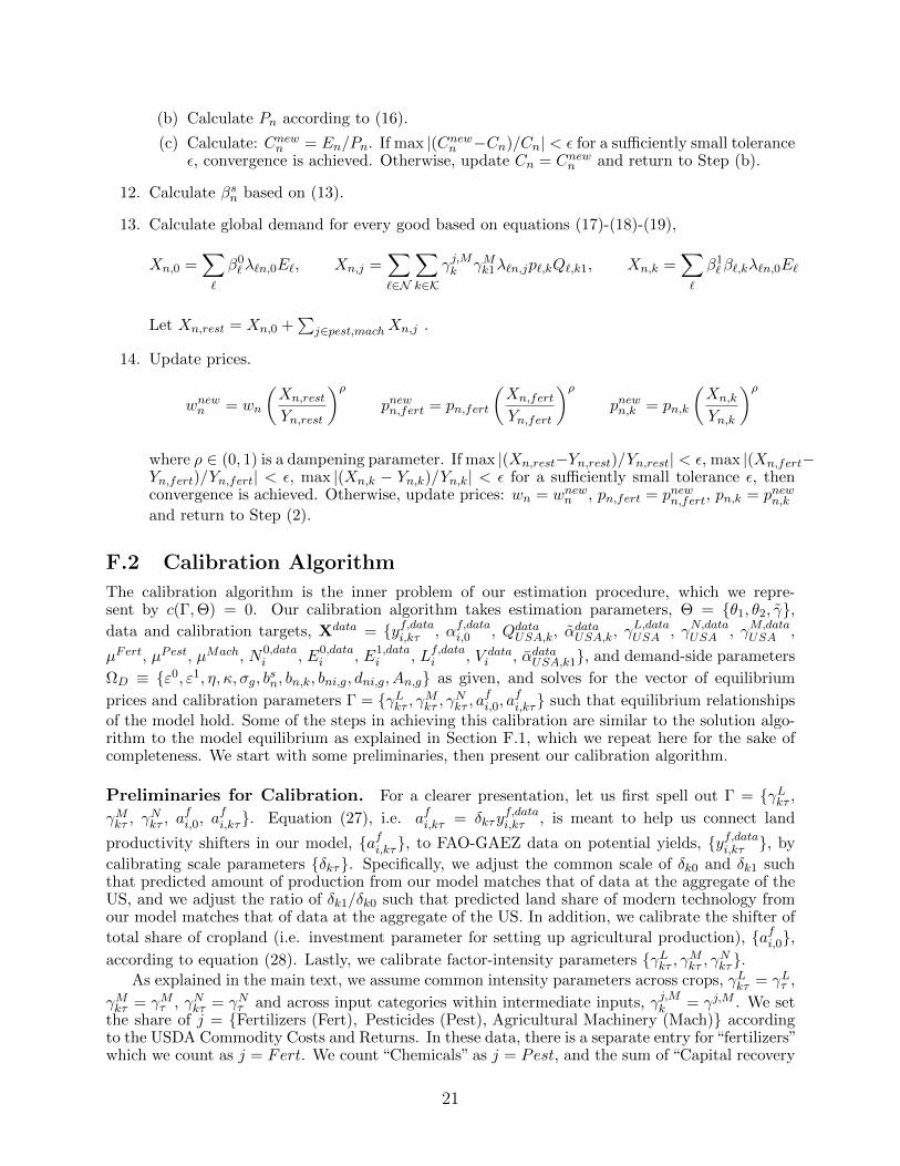
(b) Calculate Pn according to (16).

(c) Calculate: Cnewn = En/Pn. If max |(Cnewn −Cn)/Cn| < ε for a sufficiently small toleranceε, convergence is achieved. Otherwise, update Cn = Cnewn and return to Step (b).

12. Calculate βsn based on (13).

13. Calculate global demand for every good based on equations (17)-(18)-(19),

Xn,0 =∑`

β0`λ`n,0E`, Xn,j =

∑`∈N

∑k∈K

γj,Mk γMk1λ`n,jp`,kQ`,k1, Xn,k =∑`

β1`β`,kλ`n,0E`

Let Xn,rest = Xn,0 +∑

j∈pest,machXn,j .

14. Update prices.

wnewn = wn

(Xn,rest

Yn,rest

)ρpnewn,fert = pn,fert

(Xn,fert

Yn,fert

)ρpnewn,k = pn,k

(Xn,k

Yn,k

)ρwhere ρ ∈ (0, 1) is a dampening parameter. If max |(Xn,rest−Yn,rest)/Yn,rest| < ε, max |(Xn,fert−Yn,fert)/Yn,fert| < ε, max |(Xn,k − Yn,k)/Yn,k| < ε for a sufficiently small tolerance ε, thenconvergence is achieved. Otherwise, update prices: wn = wnewn , pn,fert = pnewn,fert, pn,k = pnewn,k

and return to Step (2).

F.2 Calibration Algorithm

The calibration algorithm is the inner problem of our estimation procedure, which we repre-sent by c(Γ,Θ) = 0. Our calibration algorithm takes estimation parameters, Θ = θ1, θ2, γ,data and calibration targets, Xdata = yf,datai,kτ , αf,datai,0 , QdataUSA,k, α

dataUSA,k, γ

L,dataUSA , γN,dataUSA , γM,data

USA ,

µFert, µPest, µMach, N0,datai , E0,data

i , E1,datai , Lf,datai , V data

i , αdataUSA,k1, and demand-side parameters

ΩD ≡ ε0, ε1, η, κ, σg, bsn, bn,k, bni,g, dni,g, An,g as given, and solves for the vector of equilibrium

prices and calibration parameters Γ = γLkτ , γMkτ , γNkτ , afi,0, a

fi,kτ such that equilibrium relationships

of the model hold. Some of the steps in achieving this calibration are similar to the solution algo-rithm to the model equilibrium as explained in Section F.1, which we repeat here for the sake ofcompleteness. We start with some preliminaries, then present our calibration algorithm.

Preliminaries for Calibration. For a clearer presentation, let us first spell out Γ = γLkτ ,γMkτ , γ

Nkτ , a

fi,0, a

fi,kτ. Equation (27), i.e. afi,kτ = δkτy

f,datai,kτ , is meant to help us connect land

productivity shifters in our model, afi,kτ, to FAO-GAEZ data on potential yields, yf,datai,kτ , by

calibrating scale parameters δkτ. Specifically, we adjust the common scale of δk0 and δk1 suchthat predicted amount of production from our model matches that of data at the aggregate of theUS, and we adjust the ratio of δk1/δk0 such that predicted land share of modern technology fromour model matches that of data at the aggregate of the US. In addition, we calibrate the shifter of

total share of cropland (i.e. investment parameter for setting up agricultural production), afi,0,according to equation (28). Lastly, we calibrate factor-intensity parameters γLkτ , γMkτ , γNkτ.

As explained in the main text, we assume common intensity parameters across crops, γLkτ = γLτ ,

γMkτ = γMτ , γNkτ = γNτ and across input categories within intermediate inputs, γj,Mk = γj,M . We setthe share of j = Fertilizers (Fert), Pesticides (Pest), Agricultural Machinery (Mach) accordingto the USDA Commodity Costs and Returns. In these data, there is a separate entry for“fertilizers”which we count as j = Fert. We count “Chemicals” as j = Pest, and the sum of “Capital recovery

21

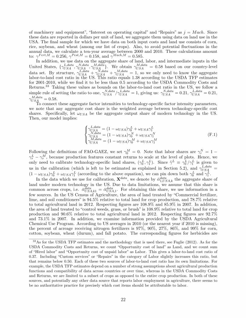
of machinery and equipment”, “Interest on operating capital” and “Repairs” as j = Mach. Sincethese data are reported in dollars per unit of land, we aggregate them using data on land use in theUSA. The final sample for which we have data on both input costs and land use consists of corn,rice, soybean, and wheat (among our list of crops). Also, to avoid potential fluctuations in theannual data, we calculate a ten-year average between 2000 and 2010. These calculations amountto: γFert,M = 0.256, γPest,M = 0.158, and γMach,M = 0.585.

In addition, we use data on the aggregate share of land, labor, and intermediate inputs in the

United States, γL,dataUSA , γN,dataUSA , γM,dataUSA . We obtain γM,data

USA = 0.58 based on our country-level

data set. By structure, γL,dataUSA + γN,dataUSA + γM,dataUSA = 1, so we only need to know the aggregate

labor-to-land cost ratio in the US. This ratio equals 1.38 according to the USDA TFP estimatesfor 2001-2010, while we find it to be less than 0.5 according to the USDA Commodity Costs andReturns.33 Taking these values as bounds on the labor-to-land cost ratio in the US, we follow a

simple rule of setting the ratio to one, γN,dataUSA /γL,dataUSA = 1, giving us: γN,dataUSA = 0.21, γL,dataUSA = 0.21,

γM,dataUSA = 0.58.

To connect these aggregate factor intensities to technology-specific factor intensity parameters,we note that any aggregate cost share is the weighted average between technology-specific costshares. Specifically, let ωUSA be the aggregate output share of modern technology in the US.Then, our model implies:

γL,dataUSA = (1− ωUSA)γL0 + ωUSAγL1

γN,dataUSA = (1− ωUSA)γN0 + ωUSAγN1

γM,dataUSA = (1− ωUSA)γM0 + ωUSAγ

M1

(F.1)

Following the definitions of FAO-GAEZ, we set γM0 = 0. Note that labor shares are γNτ = 1 −γLτ − γMτ , because production features constant returns to scale at the level of plots. Hence, weonly need to calibrate technology-specific land shares, (γL0 , γ

L1 ). Since γL ≡ γL0 /γ

L1 is given to

us in the calibration (which is left to be estimated as explained in Section 5.2), and γL,dataUSA =

(1− ωUSA)γL0 + ωUSAγL1 (according to the above equation), we can pin down both γL0 and γL1 .

In the data which we use for calibration, Xdata, we denote by αdata1,USA,k the aggregate share ofland under modern technology in the US. Due to data limitations, we assume that this share iscommon across crops, i.e. αdataUSA,k1 = αdataUSA,1. For obtaining this share, we use information in afew sources. In the US Census of Agriculture, the area of land treated by “Commercial fertilizer,lime, and soil conditioners” is 94.5% relative to total land for crop production, and 78.7% relativeto total agricultural land in 2012. Respecting figures are 108.9% and 85.9% in 2007. In addition,the area of land treated to “control weeds, grass, or brush” is 108.9% relative to total land for cropproduction and 90.6% relative to total agricultural land in 2012. Respecting figures are 92.7%and 73.1% in 2007. In addition, we examine information provided by the USDA AgriculturalChemical Use Program. According to US averages in 2010 (or the nearest year if 2010 is missing),the percent of acreage receiving nitrogen fertilizers is 97%, 90%, 27%, 86%, and 99% for corn,cotton, soybean, wheat (durum), and fall potato. The corresponding figures for herbicides are

33As for the USDA TFP estimates and the methodology that is used there, see Fuglie (2012). As for theUSDA Commodity Costs and Returns, we count “Opportunity cost of land” as Land, and we count sumof “Hired labor” and “Opportunity cost of unpaid labor” as Labor. This gives a labor-to-land cost ratio of0.37. Including “Custom services” or “Repairs” in the category of Labor slightly increases this ratio, butthat remains below 0.50. Each of these two sources of labor-to-land cost ratio has its own limitations. Forexample, the USDA TFP estimates depend on a number of strong assumptions about agricultural productionfunctions and compatibility of data across countries or over time, whereas in the USDA Commodity Costsand Returns, we are limited to a subset of crops as opposed to the entire crop production. In both of thesesources, and potentially any other data source that reports labor employment in agriculture, there seems tobe no authoritative practice for precisely which cost items should be attributable to labor.

22

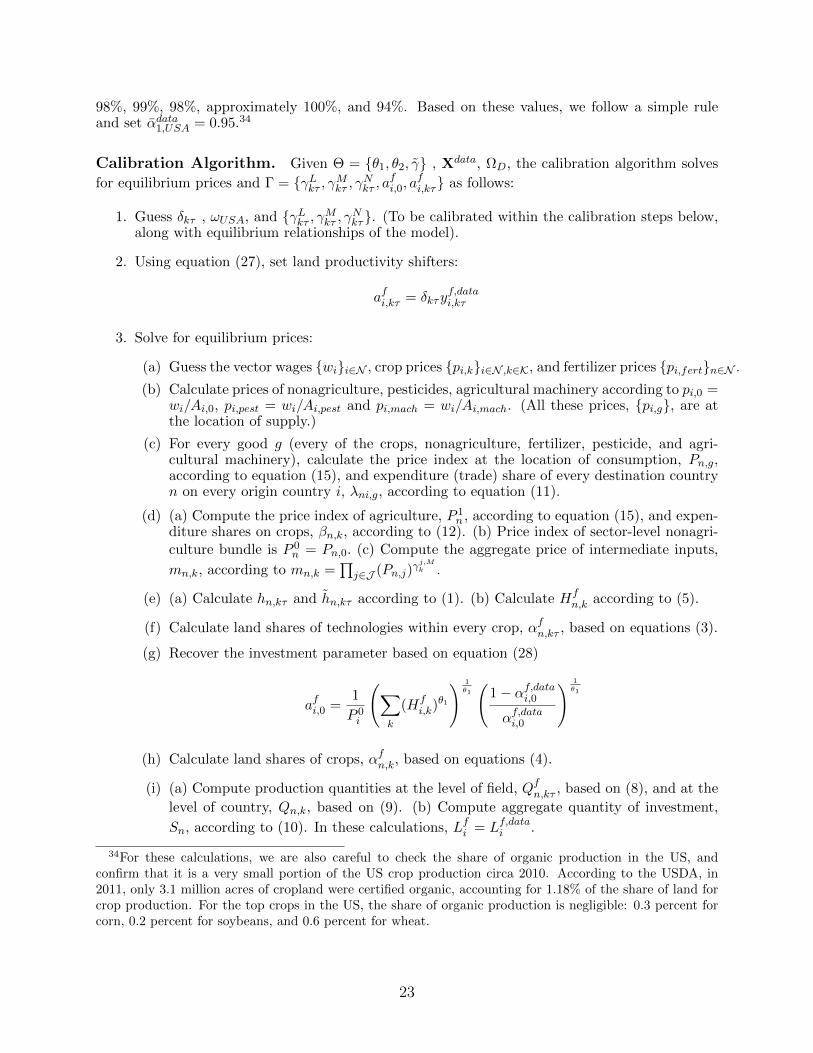
98%, 99%, 98%, approximately 100%, and 94%. Based on these values, we follow a simple ruleand set αdata1,USA = 0.95.34

Calibration Algorithm. Given Θ = θ1, θ2, γ , Xdata, ΩD, the calibration algorithm solves

for equilibrium prices and Γ = γLkτ , γMkτ , γNkτ , afi,0, a

fi,kτ as follows:

1. Guess δkτ , ωUSA, and γLkτ , γMkτ , γNkτ. (To be calibrated within the calibration steps below,along with equilibrium relationships of the model).

2. Using equation (27), set land productivity shifters:

afi,kτ = δkτyf,datai,kτ

3. Solve for equilibrium prices:

(a) Guess the vector wages wii∈N , crop prices pi,ki∈N ,k∈K, and fertilizer prices pi,fertn∈N .

(b) Calculate prices of nonagriculture, pesticides, agricultural machinery according to pi,0 =wi/Ai,0, pi,pest = wi/Ai,pest and pi,mach = wi/Ai,mach. (All these prices, pi,g, are atthe location of supply.)

(c) For every good g (every of the crops, nonagriculture, fertilizer, pesticide, and agri-cultural machinery), calculate the price index at the location of consumption, Pn,g,according to equation (15), and expenditure (trade) share of every destination countryn on every origin country i, λni,g, according to equation (11).

(d) (a) Compute the price index of agriculture, P 1n , according to equation (15), and expen-

diture shares on crops, βn,k, according to (12). (b) Price index of sector-level nonagri-culture bundle is P 0

n = Pn,0. (c) Compute the aggregate price of intermediate inputs,

mn,k, according to mn,k =∏j∈J (Pn,j)

γj,Mk .

(e) (a) Calculate hn,kτ and hn,kτ according to (1). (b) Calculate Hfn,k according to (5).

(f) Calculate land shares of technologies within every crop, αfn,kτ , based on equations (3).

(g) Recover the investment parameter based on equation (28)

afi,0 =1

P 0i

(∑k

(Hfi,k)

θ1

) 1

θ1

(1− αf,datai,0

αf,datai,0

) 1

θ1

(h) Calculate land shares of crops, αfn,k, based on equations (4).

(i) (a) Compute production quantities at the level of field, Qfn,kτ , based on (8), and at the

level of country, Qn,k, based on (9). (b) Compute aggregate quantity of investment,

Sn, according to (10). In these calculations, Lfi = Lf,datai .

34For these calculations, we are also careful to check the share of organic production in the US, andconfirm that it is a very small portion of the US crop production circa 2010. According to the USDA, in2011, only 3.1 million acres of cropland were certified organic, accounting for 1.18% of the share of land forcrop production. For the top crops in the US, the share of organic production is negligible: 0.3 percent forcorn, 0.2 percent for soybeans, and 0.6 percent for wheat.

23

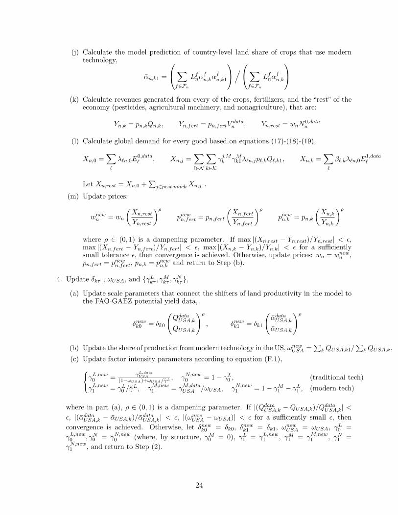
(j) Calculate the model prediction of country-level land share of crops that use moderntechnology,

αn,k1 =

∑f∈Fn

Lfnαfn,kα

fn,k1

/∑f∈Fn

Lfnαfn,k

(k) Calculate revenues generated from every of the crops, fertilizers, and the “rest” of the

economy (pesticides, agricultural machinery, and nonagriculture), that are:

Yn,k = pn,kQn,k, Yn,fert = pn,fertVdatan , Yn,rest = wnN

0,datan

(l) Calculate global demand for every good based on equations (17)-(18)-(19),

Xn,0 =∑`

λ`n,0E0,data` , Xn,j =

∑`∈N

∑k∈K

γj,Mk γMk1λ`n,jp`,kQ`,k1, Xn,k =∑`

β`,kλ`n,0E1,data`

Let Xn,rest = Xn,0 +∑

j∈pest,machXn,j .

(m) Update prices:

wnewn = wn

(Xn,rest

Yn,rest

)ρpnewn,fert = pn,fert

(Xn,fert

Yn,fert

)ρpnewn,k = pn,k

(Xn,k

Yn,k

)ρwhere ρ ∈ (0, 1) is a dampening parameter. If max |(Xn,rest − Yn,rest)/Yn,rest| < ε,max |(Xn,fert − Yn,fert)/Yn,fert| < ε, max |(Xn,k − Yn,k)/Yn,k| < ε for a sufficientlysmall tolerance ε, then convergence is achieved. Otherwise, update prices: wn = wnewn ,pn,fert = pnewn,fert, pn,k = pnewn,k and return to Step (b).

4. Update δkτ , ωUSA, and γLkτ , γMkτ , γNkτ,

(a) Update scale parameters that connect the shifters of land productivity in the model tothe FAO-GAEZ potential yield data,

δnewk0 = δk0

(QdataUSA,k

QUSA,k

)ρ, δnewk1 = δk1

(αdataUSA,k

αUSA,k

)ρ

(b) Update the share of production from modern technology in the US, ωnewUSA =∑

kQUSA,k1/∑

kQUSA,k.

(c) Update factor intensity parameters according to equation (F.1),γL,new0 = γL,dataUSA

(1−ωUSA)+ωUSA/γL, γN,new0 = 1− γL0 , (traditional tech)

γL,new1 = γL0 /γL, γM,new

1 = γM,dataUSA /ωUSA, γN,new1 = 1− γM1 − γL1 , (modern tech)

where in part (a), ρ ∈ (0, 1) is a dampening parameter. If |(QdataUSA,k − QUSA,k)/QdataUSA,k| <ε, |(αdataUSA,k − αUSA,k)/α

dataUSA,k| < ε, |(ωnewUSA − ωUSA)| < ε for a sufficiently small ε, then

convergence is achieved. Otherwise, let δnewk0 = δk0, δnewk1 = δk1, ωnewUSA = ωUSA, γL0 =

γL,new0 , γN0 = γN,new0 (where, by structure, γM0 = 0), γL1 = γL,new1 , γM1 = γM,new1 , γN1 =

γN,new1 , and return to Step (2).

24

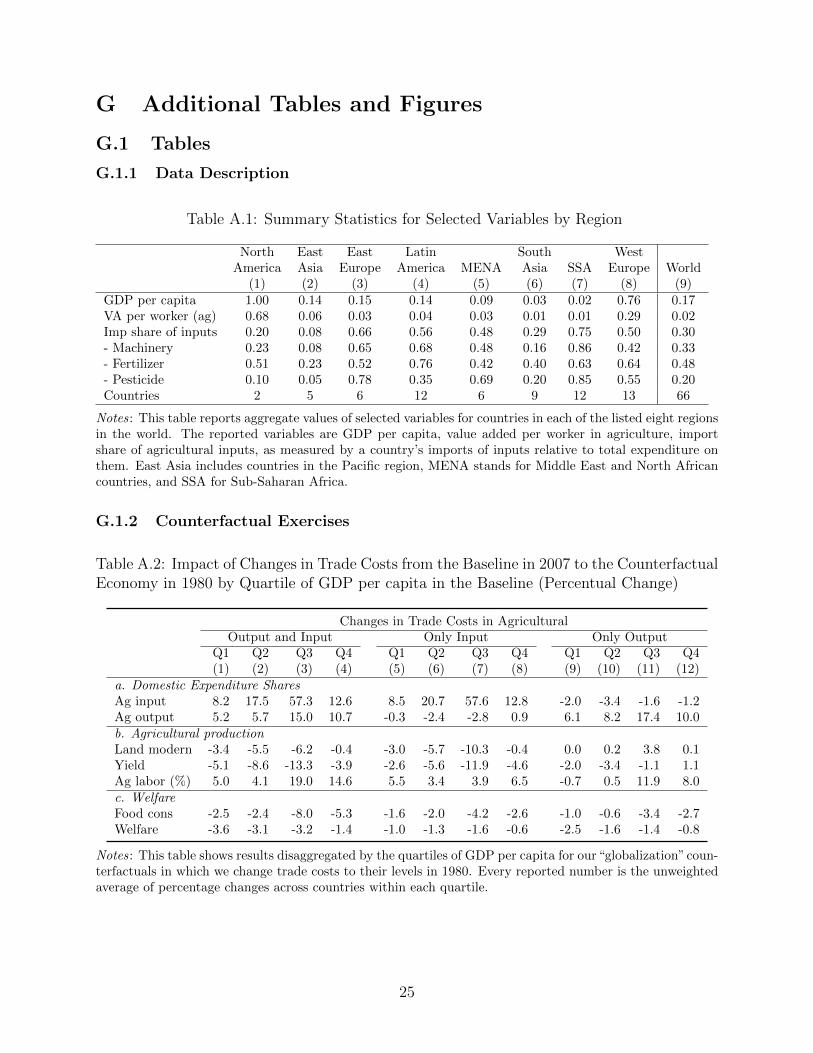
G Additional Tables and Figures

G.1 Tables

G.1.1 Data Description

Table A.1: Summary Statistics for Selected Variables by Region

North East East Latin South WestAmerica Asia Europe America MENA Asia SSA Europe World

(1) (2) (3) (4) (5) (6) (7) (8) (9)GDP per capita 1.00 0.14 0.15 0.14 0.09 0.03 0.02 0.76 0.17VA per worker (ag) 0.68 0.06 0.03 0.04 0.03 0.01 0.01 0.29 0.02Imp share of inputs 0.20 0.08 0.66 0.56 0.48 0.29 0.75 0.50 0.30- Machinery 0.23 0.08 0.65 0.68 0.48 0.16 0.86 0.42 0.33- Fertilizer 0.51 0.23 0.52 0.76 0.42 0.40 0.63 0.64 0.48- Pesticide 0.10 0.05 0.78 0.35 0.69 0.20 0.85 0.55 0.20Countries 2 5 6 12 6 9 12 13 66

Notes: This table reports aggregate values of selected variables for countries in each of the listed eight regionsin the world. The reported variables are GDP per capita, value added per worker in agriculture, importshare of agricultural inputs, as measured by a country’s imports of inputs relative to total expenditure onthem. East Asia includes countries in the Pacific region, MENA stands for Middle East and North Africancountries, and SSA for Sub-Saharan Africa.

G.1.2 Counterfactual Exercises

Table A.2: Impact of Changes in Trade Costs from the Baseline in 2007 to the CounterfactualEconomy in 1980 by Quartile of GDP per capita in the Baseline (Percentual Change)

Changes in Trade Costs in AgriculturalOutput and Input Only Input Only Output

Q1 Q2 Q3 Q4 Q1 Q2 Q3 Q4 Q1 Q2 Q3 Q4(1) (2) (3) (4) (5) (6) (7) (8) (9) (10) (11) (12)

a. Domestic Expenditure SharesAg input 8.2 17.5 57.3 12.6 8.5 20.7 57.6 12.8 -2.0 -3.4 -1.6 -1.2Ag output 5.2 5.7 15.0 10.7 -0.3 -2.4 -2.8 0.9 6.1 8.2 17.4 10.0b. Agricultural productionLand modern -3.4 -5.5 -6.2 -0.4 -3.0 -5.7 -10.3 -0.4 0.0 0.2 3.8 0.1Yield -5.1 -8.6 -13.3 -3.9 -2.6 -5.6 -11.9 -4.6 -2.0 -3.4 -1.1 1.1Ag labor (%) 5.0 4.1 19.0 14.6 5.5 3.4 3.9 6.5 -0.7 0.5 11.9 8.0c. WelfareFood cons -2.5 -2.4 -8.0 -5.3 -1.6 -2.0 -4.2 -2.6 -1.0 -0.6 -3.4 -2.7Welfare -3.6 -3.1 -3.2 -1.4 -1.0 -1.3 -1.6 -0.6 -2.5 -1.6 -1.4 -0.8

Notes: This table shows results disaggregated by the quartiles of GDP per capita for our“globalization”coun-terfactuals in which we change trade costs to their levels in 1980. Every reported number is the unweightedaverage of percentage changes across countries within each quartile.

25

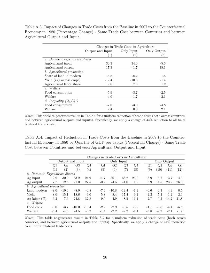
Table A.3: Impact of Changes in Trade Costs from the Baseline in 2007 to the CounterfactualEconomy in 1980 (Percentage Change) - Same Trade Cost between Countries and betweenAgricultural Output and Input

Changes in Trade Costs in AgricultureOutput and Input Only Input Only Output

(1) (2) (3)a. Domestic expenditure sharesAgricultural input 30.3 34.0 -5.3Agricultural output 17.3 -1.7 18.1b. Agricultural productionShare of land in modern -6.8 -8.2 1.5Yield (avg across crops) -12.4 -10.3 -1.4Agricultural labor share 9.6 7.3 1.2c. WelfareFood consumption -5.9 -3.7 -2.5Welfare -4.0 -1.7 -2.1d. Inequality (Q4/Q1)Food consumption -7.6 -3.0 -4.8Welfare 2.4 0.0 2.1

Notes: This table re-generates results in Table 4 for a uniform reduction of trade costs (both across countries,and between agricultural outputs and inputs). Specifically, we apply a change of 44% reduction to all finitebilateral trade costs.

Table A.4: Impact of Reduction in Trade Costs from the Baseline in 2007 to the Counter-factual Economy in 1980 by Quartile of GDP per capita (Percentual Change) - Same TradeCost between Countries and between Agricultural Output and Input

Changes in Trade Costs in AgriculturalOutput and Input Only Input Only Output

Q1 Q2 Q3 Q4 Q1 Q2 Q3 Q4 Q1 Q2 Q3 Q4(1) (2) (3) (4) (5) (6) (7) (8) (9) (10) (11) (12)

a. Domestic Expenditure SharesAg input 12.9 30.9 63.2 24.9 14.7 36.1 68.2 26.2 -3.9 -5.7 -3.7 -4.3Ag output 7.7 12.6 21.0 27.5 -0.2 -4.5 -1.0 1.9 8.9 14.5 23.2 26.0b. Agricultural productionLand modern -8.0 -10.4 -8.0 -0.8 -7.4 -10.8 -12.4 -1.3 -0.6 0.2 4.3 0.5Yield -8.0 -15.1 -18.6 -6.0 -5.8 -8.4 -17.4 -9.2 -2.3 -5.2 -1.2 2.9Ag labor (%) 6.2 7.6 24.8 32.8 9.0 4.9 8.5 11.4 -2.7 0.3 14.2 21.8c. WelfareFood cons -3.0 -3.7 -10.0 -10.4 -2.2 -2.9 -5.5 -5.2 -1.1 -0.8 -4.4 -5.8Welfare -5.4 -4.8 -4.5 -3.2 -1.4 -2.2 -2.2 -1.4 -3.8 -2.2 -2.1 -1.7

Notes: This table re-generates results in Table A.2 for a uniform reduction of trade costs (both acrosscountries, and between agricultural outputs and inputs). Specifically, we apply a change of 44% reductionto all finite bilateral trade costs.

26

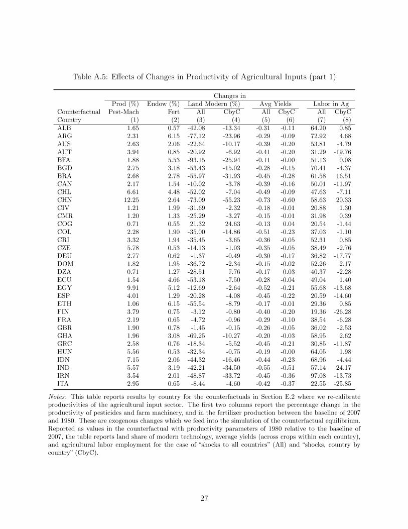
Table A.5: Effects of Changes in Productivity of Agricultural Inputs (part 1)

Changes inProd (%) Endow (%) Land Modern (%) Avg Yields Labor in Ag

Counterfactual Pest-Mach Fert All CbyC All CbyC All CbyCCountry (1) (2) (3) (4) (5) (6) (7) (8)ALB 1.65 0.57 -42.08 -13.34 -0.31 -0.11 64.20 0.85ARG 2.31 6.15 -77.12 -23.96 -0.29 -0.09 72.92 4.68AUS 2.63 2.06 -22.64 -10.17 -0.39 -0.20 53.81 -4.79AUT 3.94 0.85 -20.92 -6.92 -0.41 -0.20 31.29 -19.76BFA 1.88 5.53 -93.15 -25.94 -0.11 -0.00 51.13 0.08BGD 2.75 3.18 -53.43 -15.02 -0.28 -0.15 70.41 -4.37BRA 2.68 2.78 -55.97 -31.93 -0.45 -0.28 61.58 16.51CAN 2.17 1.54 -10.02 -3.78 -0.39 -0.16 50.01 -11.97CHL 6.61 4.48 -52.02 -7.04 -0.49 -0.09 47.63 -7.11CHN 12.25 2.64 -73.09 -55.23 -0.73 -0.60 58.63 20.33CIV 1.21 1.99 -31.69 -2.32 -0.18 -0.01 20.88 1.30CMR 1.20 1.33 -25.29 -3.27 -0.15 -0.01 31.98 0.39COG 0.71 0.55 21.32 24.63 -0.13 0.04 20.54 -1.44COL 2.28 1.90 -35.00 -14.86 -0.51 -0.23 37.03 -1.10CRI 3.32 1.94 -35.45 -3.65 -0.36 -0.05 52.31 0.85CZE 5.78 0.53 -14.13 -1.03 -0.35 -0.05 38.49 -2.76DEU 2.77 0.62 -1.37 -0.49 -0.30 -0.17 36.82 -17.77DOM 1.82 1.95 -36.72 -2.34 -0.15 -0.02 52.26 2.17DZA 0.71 1.27 -28.51 7.76 -0.17 0.03 40.37 -2.28ECU 1.54 4.66 -53.18 -7.50 -0.28 -0.04 49.04 1.40EGY 9.91 5.12 -12.69 -2.64 -0.52 -0.21 55.68 -13.68ESP 4.01 1.29 -20.28 -4.08 -0.45 -0.22 20.59 -14.60ETH 1.06 6.15 -55.54 -8.79 -0.17 -0.01 29.36 0.85FIN 3.79 0.75 -3.12 -0.80 -0.40 -0.20 19.36 -26.28FRA 2.19 0.65 -4.72 -0.96 -0.29 -0.10 38.54 -6.28GBR 1.90 0.78 -1.45 -0.15 -0.26 -0.05 36.02 -2.53GHA 1.96 3.08 -69.25 -10.27 -0.20 -0.03 58.95 2.62GRC 2.58 0.76 -18.34 -5.52 -0.45 -0.21 30.85 -11.87HUN 5.56 0.53 -32.34 -0.75 -0.19 -0.00 64.05 1.98IDN 7.15 2.06 -44.32 -16.46 -0.44 -0.23 68.96 -4.44IND 5.57 3.19 -42.21 -34.50 -0.55 -0.51 57.14 24.17IRN 3.54 2.01 -48.87 -33.72 -0.45 -0.36 97.08 -13.73ITA 2.95 0.65 -8.44 -4.60 -0.42 -0.37 22.55 -25.85

Notes: This table reports results by country for the counterfactuals in Section E.2 where we re-calibrateproductivities of the agricultural input sector. The first two columns report the percentage change in theproductivity of pesticides and farm machinery, and in the fertilizer production between the baseline of 2007and 1980. These are exogenous changes which we feed into the simulation of the counterfactual equilibrium.Reported as values in the counterfactual with productivity parameters of 1980 relative to the baseline of2007, the table reports land share of modern technology, average yields (across crops within each country),and agricultural labor employment for the case of “shocks to all countries” (All) and “shocks, country bycountry” (CbyC).

27

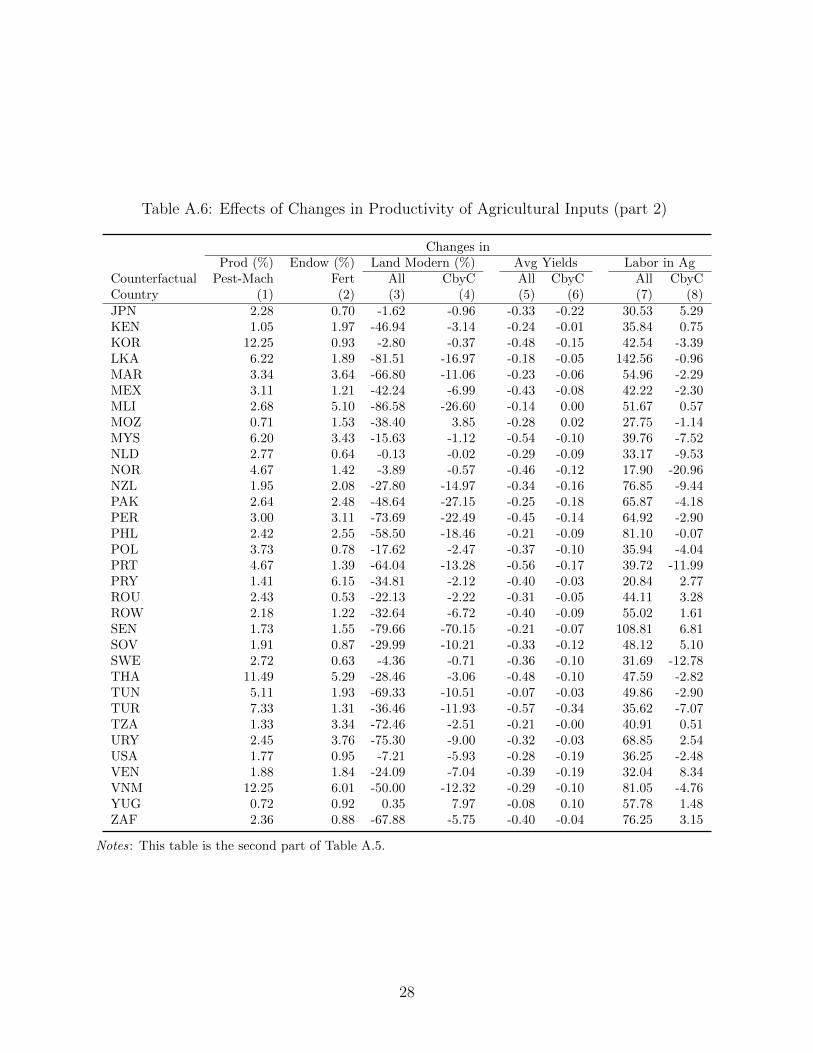
Table A.6: Effects of Changes in Productivity of Agricultural Inputs (part 2)

Changes inProd (%) Endow (%) Land Modern (%) Avg Yields Labor in Ag

Counterfactual Pest-Mach Fert All CbyC All CbyC All CbyCCountry (1) (2) (3) (4) (5) (6) (7) (8)JPN 2.28 0.70 -1.62 -0.96 -0.33 -0.22 30.53 5.29KEN 1.05 1.97 -46.94 -3.14 -0.24 -0.01 35.84 0.75KOR 12.25 0.93 -2.80 -0.37 -0.48 -0.15 42.54 -3.39LKA 6.22 1.89 -81.51 -16.97 -0.18 -0.05 142.56 -0.96MAR 3.34 3.64 -66.80 -11.06 -0.23 -0.06 54.96 -2.29MEX 3.11 1.21 -42.24 -6.99 -0.43 -0.08 42.22 -2.30MLI 2.68 5.10 -86.58 -26.60 -0.14 0.00 51.67 0.57MOZ 0.71 1.53 -38.40 3.85 -0.28 0.02 27.75 -1.14MYS 6.20 3.43 -15.63 -1.12 -0.54 -0.10 39.76 -7.52NLD 2.77 0.64 -0.13 -0.02 -0.29 -0.09 33.17 -9.53NOR 4.67 1.42 -3.89 -0.57 -0.46 -0.12 17.90 -20.96NZL 1.95 2.08 -27.80 -14.97 -0.34 -0.16 76.85 -9.44PAK 2.64 2.48 -48.64 -27.15 -0.25 -0.18 65.87 -4.18PER 3.00 3.11 -73.69 -22.49 -0.45 -0.14 64.92 -2.90PHL 2.42 2.55 -58.50 -18.46 -0.21 -0.09 81.10 -0.07POL 3.73 0.78 -17.62 -2.47 -0.37 -0.10 35.94 -4.04PRT 4.67 1.39 -64.04 -13.28 -0.56 -0.17 39.72 -11.99PRY 1.41 6.15 -34.81 -2.12 -0.40 -0.03 20.84 2.77ROU 2.43 0.53 -22.13 -2.22 -0.31 -0.05 44.11 3.28ROW 2.18 1.22 -32.64 -6.72 -0.40 -0.09 55.02 1.61SEN 1.73 1.55 -79.66 -70.15 -0.21 -0.07 108.81 6.81SOV 1.91 0.87 -29.99 -10.21 -0.33 -0.12 48.12 5.10SWE 2.72 0.63 -4.36 -0.71 -0.36 -0.10 31.69 -12.78THA 11.49 5.29 -28.46 -3.06 -0.48 -0.10 47.59 -2.82TUN 5.11 1.93 -69.33 -10.51 -0.07 -0.03 49.86 -2.90TUR 7.33 1.31 -36.46 -11.93 -0.57 -0.34 35.62 -7.07TZA 1.33 3.34 -72.46 -2.51 -0.21 -0.00 40.91 0.51URY 2.45 3.76 -75.30 -9.00 -0.32 -0.03 68.85 2.54USA 1.77 0.95 -7.21 -5.93 -0.28 -0.19 36.25 -2.48VEN 1.88 1.84 -24.09 -7.04 -0.39 -0.19 32.04 8.34VNM 12.25 6.01 -50.00 -12.32 -0.29 -0.10 81.05 -4.76YUG 0.72 0.92 0.35 7.97 -0.08 0.10 57.78 1.48ZAF 2.36 0.88 -67.88 -5.75 -0.40 -0.04 76.25 3.15

Notes: This table is the second part of Table A.5.

28

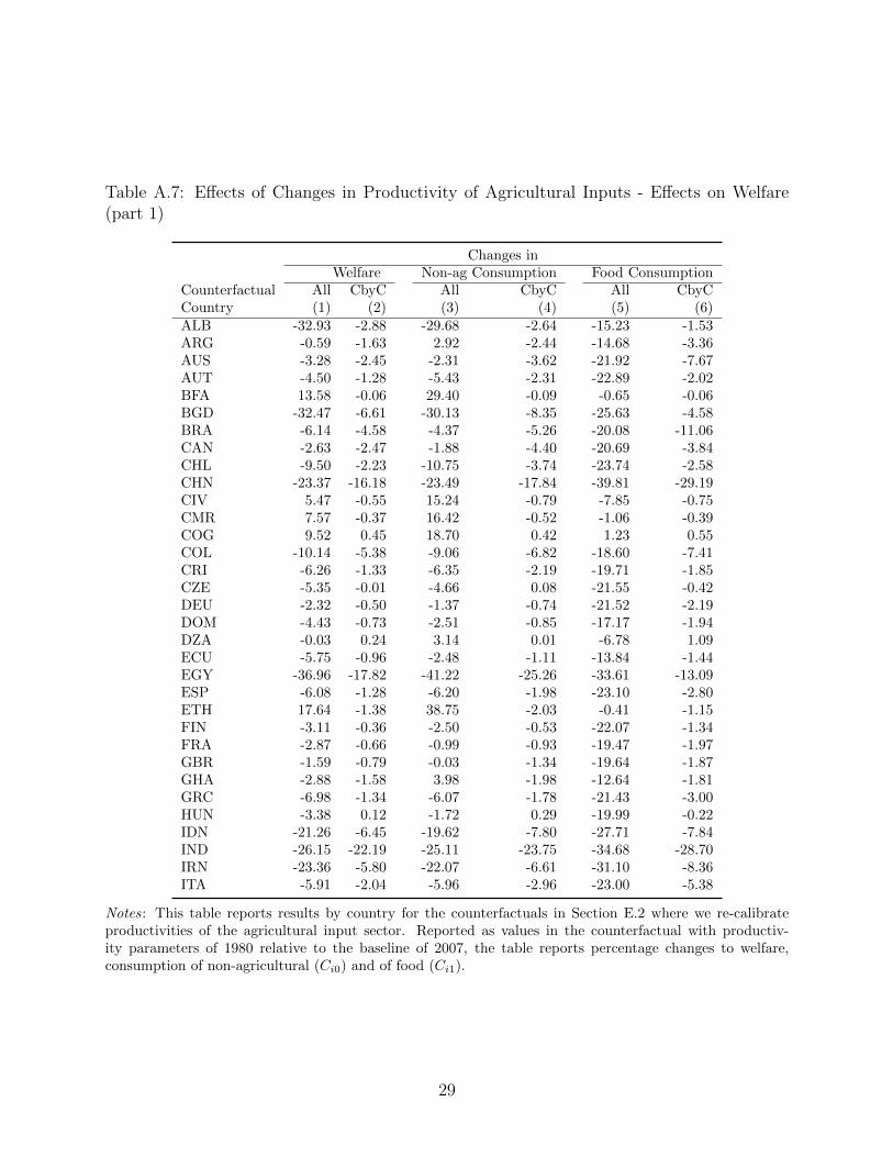
Table A.7: Effects of Changes in Productivity of Agricultural Inputs - Effects on Welfare(part 1)

Changes inWelfare Non-ag Consumption Food Consumption

Counterfactual All CbyC All CbyC All CbyCCountry (1) (2) (3) (4) (5) (6)ALB -32.93 -2.88 -29.68 -2.64 -15.23 -1.53ARG -0.59 -1.63 2.92 -2.44 -14.68 -3.36AUS -3.28 -2.45 -2.31 -3.62 -21.92 -7.67AUT -4.50 -1.28 -5.43 -2.31 -22.89 -2.02BFA 13.58 -0.06 29.40 -0.09 -0.65 -0.06BGD -32.47 -6.61 -30.13 -8.35 -25.63 -4.58BRA -6.14 -4.58 -4.37 -5.26 -20.08 -11.06CAN -2.63 -2.47 -1.88 -4.40 -20.69 -3.84CHL -9.50 -2.23 -10.75 -3.74 -23.74 -2.58CHN -23.37 -16.18 -23.49 -17.84 -39.81 -29.19CIV 5.47 -0.55 15.24 -0.79 -7.85 -0.75CMR 7.57 -0.37 16.42 -0.52 -1.06 -0.39COG 9.52 0.45 18.70 0.42 1.23 0.55COL -10.14 -5.38 -9.06 -6.82 -18.60 -7.41CRI -6.26 -1.33 -6.35 -2.19 -19.71 -1.85CZE -5.35 -0.01 -4.66 0.08 -21.55 -0.42DEU -2.32 -0.50 -1.37 -0.74 -21.52 -2.19DOM -4.43 -0.73 -2.51 -0.85 -17.17 -1.94DZA -0.03 0.24 3.14 0.01 -6.78 1.09ECU -5.75 -0.96 -2.48 -1.11 -13.84 -1.44EGY -36.96 -17.82 -41.22 -25.26 -33.61 -13.09ESP -6.08 -1.28 -6.20 -1.98 -23.10 -2.80ETH 17.64 -1.38 38.75 -2.03 -0.41 -1.15FIN -3.11 -0.36 -2.50 -0.53 -22.07 -1.34FRA -2.87 -0.66 -0.99 -0.93 -19.47 -1.97GBR -1.59 -0.79 -0.03 -1.34 -19.64 -1.87GHA -2.88 -1.58 3.98 -1.98 -12.64 -1.81GRC -6.98 -1.34 -6.07 -1.78 -21.43 -3.00HUN -3.38 0.12 -1.72 0.29 -19.99 -0.22IDN -21.26 -6.45 -19.62 -7.80 -27.71 -7.84IND -26.15 -22.19 -25.11 -23.75 -34.68 -28.70IRN -23.36 -5.80 -22.07 -6.61 -31.10 -8.36ITA -5.91 -2.04 -5.96 -2.96 -23.00 -5.38

Notes: This table reports results by country for the counterfactuals in Section E.2 where we re-calibrateproductivities of the agricultural input sector. Reported as values in the counterfactual with productiv-ity parameters of 1980 relative to the baseline of 2007, the table reports percentage changes to welfare,consumption of non-agricultural (Ci0) and of food (Ci1).

29

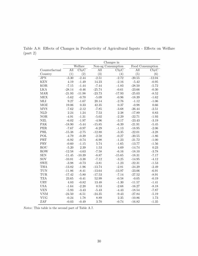
Table A.8: Effects of Changes in Productivity of Agricultural Inputs - Effects on Welfare(part 2)

Changes inWelfare Non-ag Consumption Food Consumption

Counterfactual All CbyC All CbyC All CbyCCountry (1) (2) (3) (4) (5) (6)JPN -3.30 -2.44 -2.51 -2.72 -20.55 -12.04KEN 4.19 -1.49 14.23 -2.16 -5.42 -0.95KOR -7.15 -1.44 -7.44 -1.83 -28.50 -5.72LKA -28.14 -0.46 -25.74 -0.61 -23.66 -0.30MAR -21.93 -11.98 -23.73 -17.93 -25.03 -8.52MEX -5.62 -0.70 -5.09 -0.96 -18.39 -1.62MLI 9.27 -1.67 20.14 -2.76 -1.12 -1.06MOZ 19.06 0.33 42.35 0.37 -0.98 0.66MYS -7.62 -2.12 -7.85 -3.68 -26.44 -2.51NLD 2.24 1.24 7.53 2.38 -17.89 0.83NOR -4.91 -1.31 -5.02 -2.29 -22.71 -1.93NZL -6.02 -1.97 -4.96 -3.17 -23.43 -3.19PAK -18.90 -5.44 -15.85 -6.39 -21.91 -5.45PER -7.67 -0.97 -6.29 -1.13 -18.95 -2.06PHL -15.38 -2.75 -12.88 -3.35 -22.01 -3.28POL -4.79 -0.39 -2.58 -0.27 -20.55 -1.86PRT -6.92 -0.74 -6.98 -1.23 -21.72 -1.00PRY -0.60 -1.15 5.74 -1.65 -13.77 -1.56ROU -5.20 2.39 1.53 4.69 -14.74 0.23ROW -12.58 -4.63 -7.58 -6.16 -18.10 -3.78SEN -11.45 -10.39 -8.87 -15.65 -18.31 -7.17SOV -10.81 -3.38 -7.12 -3.25 -14.95 -4.12SWE -3.98 -0.73 -3.81 -1.23 -22.31 -1.53THA -13.82 -1.96 -13.74 -2.81 -24.29 -2.49TUN -11.86 -8.41 -13.64 -13.97 -23.06 -6.91TUR -17.42 -5.80 -17.53 -7.14 -27.52 -8.91TZA 23.65 -0.41 52.99 -0.58 -0.05 -0.19URY 4.83 -0.82 13.48 -1.30 -11.57 -1.41USA -1.64 -2.20 0.53 -2.68 -16.27 -8.18VEN -5.93 -3.43 -5.43 -4.43 -18.54 -7.87VNM -24.50 -6.51 -24.35 -9.43 -27.84 -5.19YUG -0.24 1.78 8.89 2.35 -10.86 1.73ZAF -0.03 -0.49 3.70 -0.74 -16.82 -1.35

Notes: This table is the second part of Table A.7.

30

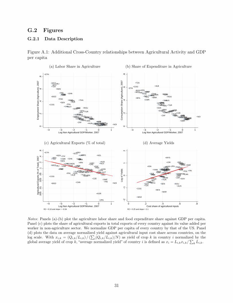
G.2 Figures

G.2.1 Data Description

Figure A.1: Additional Cross-Country relationships between Agricultural Activity and GDPper capita

(a) Labor Share in Agriculture

ALB

ARG

AUSAUT

BFA

BGD

BRA

CAN

CHLCHN

CIVCMR

COG

COL

CRI

CZEDEU

DOMDZA

ECUEGY

ESP

ETH

FINFRAGBR

GHA

GRC

HUN

IDN

IND

IRN

ITAJPN

KEN

KOR

LKA

MAR

MEX

MLIMOZ

MYS

NLD NORNZL

PAK

PER

PHL

POLPRT

PRY ROU

ROW

SEN

SOV

SWE

THA

TUN

TUR

TZA

URY

USA

VEN

VNM

YUG

ZAF

0.2

.4.6

.8E

mpl

oym

ent S

hare

(A

gric

ultu

re),

200

7

−4 −3 −2 −1 0 1Log Non Agricultural GDP/Worker, 2007

(b) Share of Expenditure in Agriculture

ALB

ARG

AUSAUT

BFA

BGD

BRA

CAN

CHL

CHN

CIV

CMR

COG

COL

CRICZE

DEU

DOM

DZA

ECU

EGY

ESP

ETH

FINFRA

GBR

GHA

GRCHUN

IDNIND

IRN

ITAJPN

KEN

KOR

LKAMAR

MEX

MLIMOZ

MYS

NLD

NORNZL

PAK

PER

PHL

POL

PRT

PRY

ROUROW

SEN

SOV

SWE

THA

TUN TUR

TZA

URY

USA

VEN

VNM

YUG

ZAF

0.2

.4.6

.8C

onsu

mpt

ion

Sha

re (

Agr

icul

ture

), 2

007


(c) Agricultural Exports (% of total)

ALB

ARG

AUS

AUT

BFA

BGD

BRA

CAN

CHL

CHN

CIV

CMR

COG

COLCRI

CZE

DEU

DOM

DZA

ECU

EGYESP

ETH

FIN

FRA

GBR

GHA

GRC

HUN

IDN

IND

IRN

ITA

JPN

KEN

KOR

LKAMAR

MEX

MLIMOZ

MYS

NLD

NOR

NZL

PAK

PER

PHL

POLPRT

PRY

ROU

ROW

SEN

SOV

SWE

THA

TUN TUR

TZA

URY

USA

VEN

VNM

YUG

ZAF

.005

.01

.025

.05

.1.2

.4.8

Agr

icul

tura

l Exp

orts

(%

of T

otal

), 2

007


R2 = 0.16 and slope = −0.34

(d) Average Yields

ALB

ARG

AUS

AUT

BFA

BGDBRA

CAN

CHLCHN

CIVCMR

COG

COL

CRI

CZE

DEU

DOM

DZA

ECUEGYESP

ETH

FIN

FRAGBR

GHA

GRC HUN

IDN

INDIRN

ITA

JPN

KEN

KOR

LKA

MAR

MEX

MLI

MOZ

MYS

NLD

NOR

NZL

PAKPER

PHL

POL

PRT

PRY

ROU

ROW

SEN

SOV

SWE

THA

TUN

TUR

TZA

URY USA

VEN

VNM

YUG

ZAF

−2

−1

01

2Lo

g of

Yie

lds

0 .2 .4 .6 .8Cost share of agricultural inputs

R2 = 0.25 and slope = 2.1

Notes: Panels (a)-(b) plot the agriculture labor share and food expenditure share against GDP per capita.Panel (c) plots the share of agricultural exports in total exports of every country against its value added perworker in non-agriculture sector. We normalize GDP per capita of every country by that of the US. Panel(d) plots the data on average normalized yield against agricultural input cost share across countries, on thelog scale. With xi,k = (Qi,k/Li,k) / (

∑i(Qi,k/Li,k)/N) as yield of crop k in country i normalized by the

global average yield of crop k, “average normalized yield” of country i is defined as xi = Li,kxi,k/∑k Li,k.

31

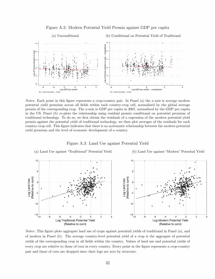
Figure A.2: Modern Potential Yield Premia against GDP per capita

(a) Unconditional−

2−

10

12

3Lo

g of

Pre

mia

(re

lativ

e to

avg

)


R2 = 0.001 and slope = −0.019

(b) Conditional on Potential Yield of Traditional

−2

−1

01

23

Log

of P

rem

ia (

rela

tive

to a

vg)

− r

esid

ualiz

ed

−4 −2 0 2 4Log GDP per worker − residualized

R2 = 0.001 and slope = −0.016

Notes: Each point in this figure represents a crop-country pair. In Panel (a) the y-axis is average modernpotential yield premium across all fields within each country-crop cell, normalized by the global averagepremia of the corresponding crop. The x-axis is GDP per capita in 2007, normalized by the GDP per capitain the US. Panel (b) re-plots the relationship using residual premia conditional on potential premium oftraditional technology. To do so, we first obtain the residuals of a regression of the modern potential yieldpremia against the potential yield of traditional technology, we then plot averages of the residuals for eachcountry-crop cell. This figure indicates that there is no systematic relationship between the modern potentialyield premium and the level of economic development of a country.

Figure A.3: Land Use against Potential Yield

(a) Land Use against “Traditional” Potential Yield (b) Land Use against “Modern” Potential Yield

Notes: This figure plots aggregate land use of crops against potential yields of traditional in Panel (a), and

of modern in Panel (b). The average country-level potential yield of a crop is the aggregate of potential

yields of the corresponding crop in all fields within the country. Values of land use and potential yields of

every crop are relative to those of corn in every country. Every point in the figure represents a crop-country

pair and those of corn are dropped since their logs are zero by structure.

32

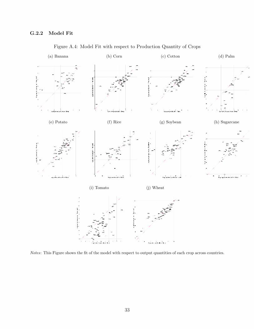
G.2.2 Model Fit

Figure A.4: Model Fit with respect to Production Quantity of Crops

(a) Banana (b) Corn (c) Cotton (d) Palm

(e) Potato (f) Rice (g) Soybean (h) Sugarcane

(i) Tomato (j) Wheat

Notes: This Figure shows the fit of the model with respect to output quantities of each crop across countries.

33

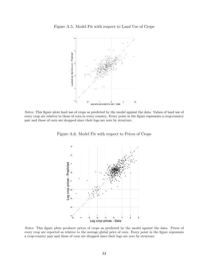
Figure A.5: Model Fit with respect to Land Use of Crops

Notes: This figure plots land use of crops as predicted by the model against the data. Values of land use ofevery crop are relative to those of corn in every country. Every point in the figure represents a crop-countrypair and those of corn are dropped since their logs are zero by structure.

Figure A.6: Model Fit with respect to Prices of Crops

Notes: This figure plots producer prices of crops as predicted by the model against the data. Prices ofevery crop are reported as relative to the average global price of corn. Every point in the figure representsa crop-country pair and those of corn are dropped since their logs are zero by structure.

34

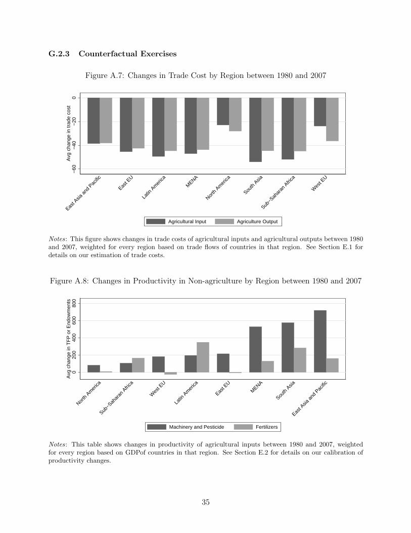
G.2.3 Counterfactual Exercises

Figure A.7: Changes in Trade Cost by Region between 1980 and 2007−

60−

40−

200

Avg

cha

nge

in tr

ade

cost

East A

sia a

nd P

acific

East E

U

Latin

Am

erica

MENA

North

Am

erica

South

Asia

Sub−S

ahar

an A

frica

Wes

t EU

Agricultural Input Agriculture Output

Notes: This figure shows changes in trade costs of agricultural inputs and agricultural outputs between 1980and 2007, weighted for every region based on trade flows of countries in that region. See Section E.1 fordetails on our estimation of trade costs.

Figure A.8: Changes in Productivity in Non-agriculture by Region between 1980 and 2007

020

040

060

080

0A

vg c

hang

e in

TF

P o

r E

ndow

men

ts

North

Am

erica

Sub−S

ahar

an A

frica

Wes

t EU

Latin

Am

erica

East E

U

MENA

South

Asia

East A

sia a

nd P

acific

Machinery and Pesticide Fertilizers

Notes: This table shows changes in productivity of agricultural inputs between 1980 and 2007, weightedfor every region based on GDPof countries in that region. See Section E.2 for details on our calibration ofproductivity changes.

35

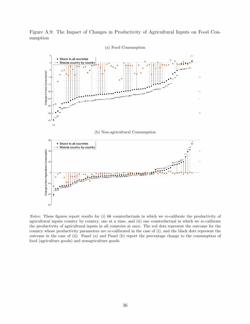
Figure A.9: The Impact of Changes in Productivity of Agricultural Inputs on Food Con-sumption

(a) Food Consumption

(b) Non-agricultural Consumption

Notes: These figures report results for (i) 66 counterfactuals in which we re-calibrate the productivity ofagricultural inputs country by country, one at a time, and (ii) one counterfactual in which we re-calibratethe productivity of agricultural inputs in all countries at once. The red dots represent the outcome for thecountry whose productivity parameters are re-calibrated in the case of (i), and the black dots represent theoutcome in the case of (ii). Panel (a) and Panel (b) report the percentage change to the consumption offood (agriculture goods) and nonagriculture goods.

36

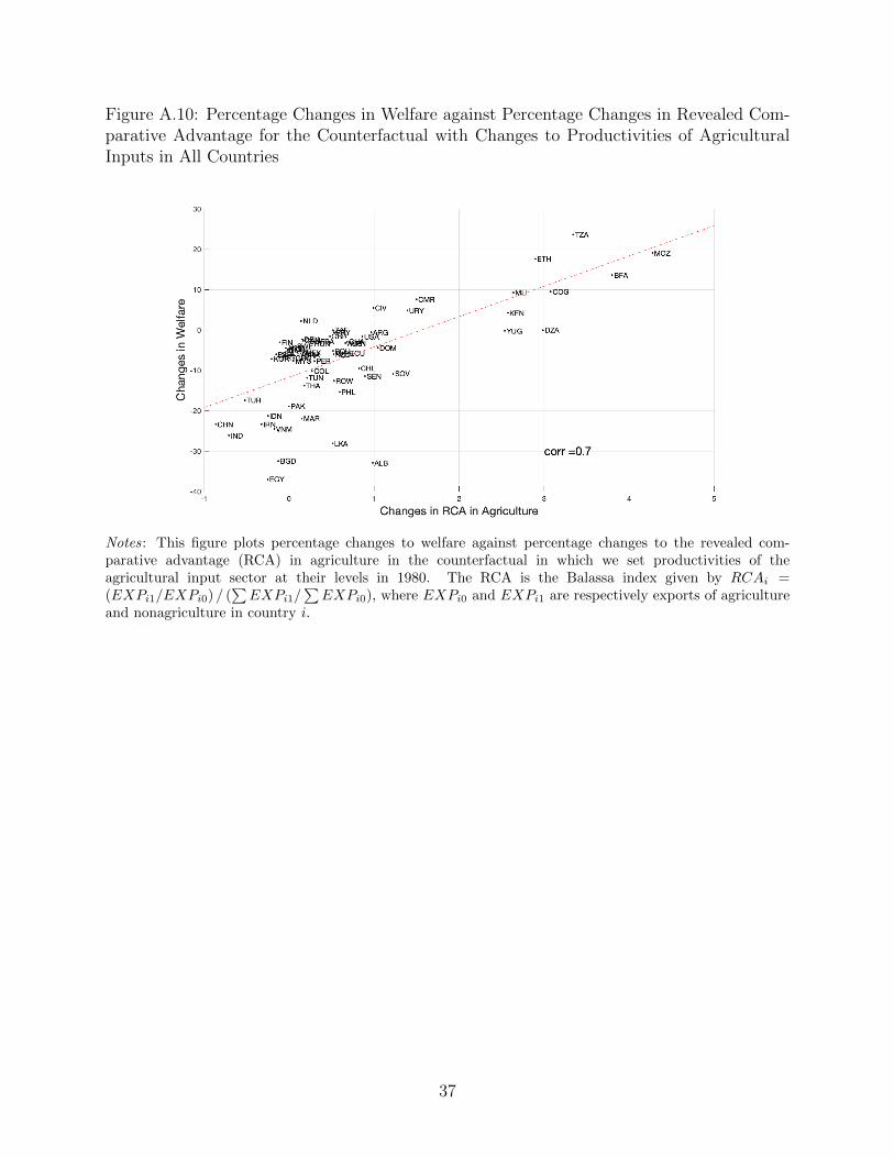
Figure A.10: Percentage Changes in Welfare against Percentage Changes in Revealed Com-parative Advantage for the Counterfactual with Changes to Productivities of AgriculturalInputs in All Countries

Notes: This figure plots percentage changes to welfare against percentage changes to the revealed com-parative advantage (RCA) in agriculture in the counterfactual in which we set productivities of theagricultural input sector at their levels in 1980. The RCA is the Balassa index given by RCAi =(EXPi1/EXPi0) / (

∑EXPi1/

∑EXPi0), where EXPi0 and EXPi1 are respectively exports of agriculture

and nonagriculture in country i.

37

Trade, Technology, and Agricultural Productivity

Documents