Trade, Relative Prices, and the Canadian Great Depression

Trade, Relative Prices, and the Canadian Great Depression∗

Pedro S. Amaral

Federal Reserve Bank of Cleveland

James C. MacGee

Western University

September 30, 2016

Abstract

Canadian GNP per capita fell by roughly a third between 1928 and 1933. Although the

decline and the slow recovery of GNP resemble the American Great Depression, trade was more

important in Canada, as exports and imports each accounted for roughly a quarter of Canadian

GNP in 1928. The fall in the trade share of GNP of roughly 30 percent between 1928 and 1933

was accompanied by a decline of over 20 percent in the relative prices of exports and imports

relative to nontraded goods. We develop a three-sector small open economy model, where wages

in the nontraded and import competing sectors adjust slowly due to Taylor contracts. We feed

the relative prices of imports and exports from the data into the model, and find that the fall in

traded goods prices can account for roughly half of the fall in GNP during the Canadian Great

Contraction.

JEL Classification: E20, E30, E50.

Keywords: Great Depression, Sectoral Models, Trade, Relative Prices, Sticky Wages.

∗We thank workshop participants at the Federal Reserve Bank of Cleveland and Western for helpful comments.This research was supported by the Social Science and Humanities Research Council of Canada grant “Trade, RelativePrices and the Great Depression”. The views expressed herein are those of the authors and not necessarily thoseof the Federal Reserve Bank of Cleveland or the Federal Reserve System. Corresponding Author: Jim MacGee,Department of Economics, Western University, Social Science Centre, London, Ontario, N6A 5C2, fax: (519) 6613666, e-mail: [email protected].

1

1 Introduction

A common view is that fixed exchange rates (i.e., the gold standard) played a key factor in the

international transmission of the Great Depression.1 In this story, the transmission mechanism

involves an explicit change in the price level which occurs (at least partly) via trade. However,

surprisingly little work has attempted to quantify the impact of the fall in prices of traded goods

during the Great Depression.

In this paper, we quantify the role of falling prices of traded goods in the transmission of the

Great Depression to Canada. Canada is an interesting country to examine for several reasons.

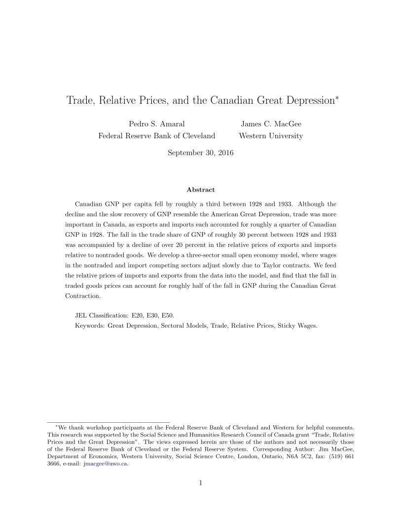
First, the path of real GDP per capita closely parallels that of the U.S. over 1928-1933, as well

as during the protracted post 1933 recovery (see Figure 1). Second, it was (and is) a small open

economy, with trade accounting for a large share of the economy. In addition, while it closely

resembles the U.S. in many ways, it neither experienced a banking crisis, as Haubrich (1990) notes,

nor did it implement many of the New Deal policies analyzed in Cole and Ohanian (2004).2 Finally,

there is substantial data to guide our analysis, since the Dominion Bureau of Statistics collected

and published data on prices, quantities and employment at both the sectoral and aggregate levels.

Our first contribution is to document the substantial shifts in relative price and wages across

industries. While the fall in the prices of commodities relative to finished goods during the De-

pression is well known (e.g., see Lewis (1949) and Safarian (1970)), the large rise in the price of

nontraded goods relative to traded goods has remained largely undiscussed. We show that this shift

in relative prices was accompanied by a shift in relative wages, as wages in the nontraded sector rose

relative to traded industries. However, the fall in employment and real output varied substantially

across industries, with employment in agriculture (which accounted for roughly a third of Canadian

workers at the beginning of the Depression and was the largest source of exports) not declining

despite a fall in wages of nearly 50 percent.

This large shift in wages and prices of nontraded relative to traded goods motivates our quan-

titative model. We develop a small open economy model with two traded sectors – one export and

one import-competing – as well as a nontraded sector. Each of the sectoral goods is produced using

an immobile factor (capital) and labor. The final consumption good is produced using all three

sectoral goods. Although workers face a labor-leisure trade-off, we assume they cannot move be-

tween industries.3 In our numerical experiments, we choose parameter values to match the sectoral

1See Temin (1993), Eichengreen (1992), and Eichengreen (1995).2See Amaral and MacGee (2002) for a comparison between the American and Canadian economies in the Great

Depression.3This is broadly consistent with the data, as there is little evidence of large flows of workers across industries. This

could reflect geographical frictions, as agricultural workers were disproportionately located in the Prairie Provinces.

2

and trade shares from 1926, when agricultural yields were near historical averages.4

To illustrate the puzzle of the large shift in the relative price of traded to nontraded goods,

we feed the prices of export and imported goods from the data into the model. We find that the

model predicts a large decline in nontraded prices, and hence little change in relative prices or

wages across sectors. The small fall in output is consistent with Amaral and MacGee (2002), who

also find that the adverse movement in the terms of trade accounts for a small fraction of the fall

in output during the Great Depression.

This discrepancy between the relative prices of traded and nontraded goods predicted by this

frictionless model and observed in the data leads us to introduce (Taylor) nominal wage contracts

in the nontraded and import competing sectors. In these sectors, hours worked are determined by

the short side of the market, which for the shocks we consider implies they depend on the firms’ real

product wage. In the export competing sector, wages adjust to equate labor demand and supply.

Our benchmark counterfactual features two sets of shocks. The first are shocks to the prices

of export and import competing goods, which we take from the data. Given the large share of

agricultural products (especially wheat) in Canadian exports, we account for low agricultural yields

by inputting a real shock to the export sector. This shock is calibrated to match the implications

of variations in yields of the main field crops for average productivity in the export sector. The key

wage rigidity parameters are calibrated so as to match the sectoral real product wages. Although

we do not directly target it, our benchmark implies a path for the nontraded good price similar to

that observed in the data. In turn, given that we feed in the prices of export and import competing

goods, this implies that our benchmark average price is similar to that of the GNP Deflator.

We find that the large change in the relative prices of traded and nontraded goods can account

for over half of the fall in output during the Canadian Great Depression. The fall in real output is

driven by the import competing and nontraded sectors. In both sectors, the fall in output is driven

by an increase in the real product wage which leads to a fall in labor. The model also implies a

large decline in measured labour productivity.

Motivated by the large literature that assesses the contribution of deflation and wage rigidity

to the Great Depression (see Bordo, Erceg, and Evans (2000)), we analyze a counterfactual where

we feed in a monetary shock constructed to match the fall in Canadian M1. Since a contractionary

monetary shock lowers prices, in this experiment we lower the magnitude of the international price

shock so that we hit the same path for prices as in our benchmark. We find that adding the

monetary shock has little impact on the predicted decline in output. This finding is consistent

with Betts, Bordo, and Redish (1996) and Amaral and MacGee (2002), who also conclude that

4This is done to avoid calibrating to the historically high crop yields in 1928 or the initial decline in prices oftraded goods.

3

real, rather than monetary shocks were the key driver of the fall in output in the Canadian Great

Depression.

Our work is related to a long standing literature which argues that international trade was an

important factor in the transmission of the Great Depression to Canada.5 In early narrative work,

Safarian (1970), Mackintosh (1964) and Marcus (1954) argue that the large decline in agricultural

prices and exports played a significant role in the Canadian Great Depression. In contrast, Amaral

and MacGee (2002) find that in a small open economy version of the standard international real

business cycle models of Backus, Kehoe, and Kydland (1995), the shifts in the terms of trade

account for only a small fraction of the decline in output over 1929 to 1933. This paper helps to

reconcile these divergent views, as we show that the main effects of the fall in the international price

of traded goods did not come about because of a shift in the terms of trade, but rather because of

the large fall in the price of traded relative to nontraded goods.

Our paper contributes to a broader literature examining the international transmission of the

Great Depression. In common with Madsen (2001), our results suggest that the decline in agri-

cultural prices played a key role in the transmission of the Great Depression across countries. In

recent work, Cole, Ohanian, and Leung (2007) revisit the conclusions of Eichengreen and Sachs

(1985) and Bernanke and Carey (1996) that different timing in abandoning the international gold

standard accounts for the observed cross-country deflations and output declines. They find evi-

dence of the former, but not the latter causal relationship. Instead, they conclude that a decline in

measured productivity accounts for roughly two-thirds of the decline in output, with the tradable

sector playing an important role in the varying severity across countries. Green and Sparks (1988)

argue that Canada’s larger fall in output was due to its closer relationship with the U.S., while

Australia benefited from its close ties with England. Our work points to an important relationship

between relative prices and the impact of the Great Depression.6

Our paper is also related to a broader literature exploring the impact of shifts in relative prices

on the real economy. Kose (2002) uses a two-sector small open economy model to decompose the

impact of shocks to the prices of developing economies, and finds that they account for a significant

share of the volatility of GDP. Ball and Mankiw (1995) argue that relative price shocks combined

with slow price adjustment can have an impact similar to that of supply shocks. While our paper

5See, for examples, Safarian (1970), Marcus (1954), Green and Sparks (1988).6Our finding is also consistent with Amaral and MacGee (2015), who conclude that real wage rigidities combined

with deflation account for less than a fifth of the fall in output the U.S. Great Contraction. This work shareswith Cole and Ohanian (2001) the view that taking sectoral heterogeneity in wages into account is important.Interestingly, Ohanian (2009) argues that the threat of unionization in manufacturing allowed President Hoover toconvince manufacturing firms to keep their wages high while reducing the length of their workweek in exchange forprotection from unions. Inputting the observed wages and workweek length in manufacturing and agriculture into atwo-sector model, he is able to generate two-thirds of the fall in output by the end of 1931.

4

also examines the quantitative importance of relative price shocks, we differ both in our modeling

approach as well as in our focus on the interwar period.

The remainder of this paper is organized as follows. Section 2 documents several key facts on

relative prices, quantities and trade flows during the Great Depression. Section 3 outlines the small

open economy model environment we use to quantify the effect of price shocks on the Canadian

economy. Section 4 summarizes the findings of our counterfactual experiments. The final section

offers a brief conclusion.

2 Key Facts from the Data

We begin by documenting several facts. First, there were large changes in relative prices, with

a large fall in the relative price of traded to nontraded goods. In addition, the price of export

goods fell relative to import goods. This shift in the terms of trade was largely due to a fall in the

price of commodities relative to manufactured goods, as Canada was a net exporter of commodities

(especially agricultural and forestry products) and an importer of manufactured goods. Second,

these shifts in relative prices were accompanied by large shifts in relative wages across sectors, with

nontraded wages rising relative to traded sector wages. Third, the traded good share of GDP in

Canada fell during 1928-33. Finally, the large fall in the price of agricultural commodities did not

lead to a reallocation of workers as there was little labor movement away from agriculture.

We also briefly outline some facts that help to rationalize these observations. First, we document

that some (mainly nontraded) industries’ prices were regulated and that these regulated prices

adjusted slowly during the 1930s. Second, the large fall in commodity prices coincided with a large

decline in the world price of agricultural and forestry prices. Third, this decline in agricultural

prices during the late 1920s and 1930s was accentuated by substantial increases in tariffs and trade

barriers in Western European countries. In addition, several large exporters moved to subsidize

domestic production and export of commodities. Finally, the end of the 1930s witnessed the return

of the USSR to world export markets.

2.1 Sectoral Shares of GNP and Trade

Before setting out facts on sectoral prices, wages and trade, we first outline our division of industries

and their share of nominal GDP during the Great Depression.

We divide industries into nontraded, export and import-competing based on net trade flows.

At the beginning of the Great Depression, Canada was a major exporter of agricultural and nat-

ural resource goods (both raw and processed). This leads us to classify Agriculture, Fishing and

Forestry and Mining as export industries. We also classify the manufacturing industries Food and

5

Beverages and Wood and Paper as exporters, since processed goods such as (wheat) flour and wood

pulp accounted for a significant share of exports. We classify the remaining manufacturing indus-

tries as import-competing, since Canada was a net importer of manufactured goods (particularly

investment goods), mainly from the United States. Finally, the nontraded industries are Retail and

Wholesale Trade, Government, Finance, Insurance and Real Estate, Transportation, Utilities and

Communication, Services and Construction.

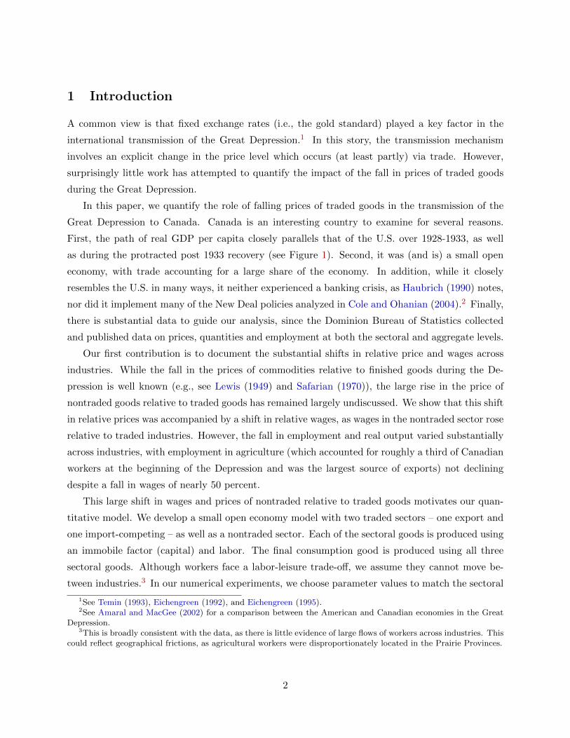
Figure 2 plots the nominal share of GDP for our three-sector classification. A key take-away

from the figure is the large fall in the tradable sector share of GDP over 1926-33. This was mainly

due to a decline in the export industries, particularly agriculture, whose share of GDP fell from

roughly 17% over 1926-28 to less than 10% by 1933. While the government share of GDP did rise

during the Depression, it played a small role in the rise in the nontradable share of GDP, as the

share of government in GDP only rose from 5% in 1929 to roughly 7% over 1933-39.

2.2 Decline in Trade

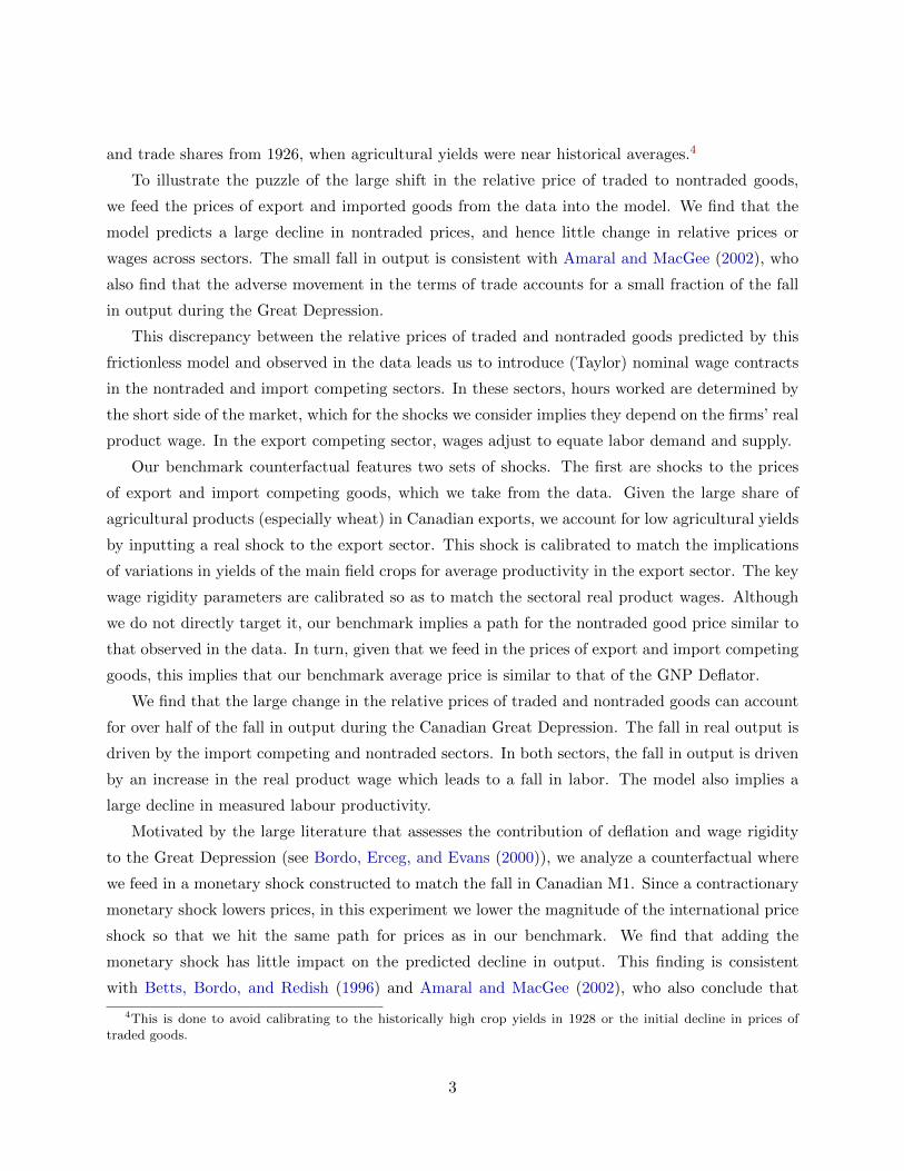
The decline in Canadian exports and imports between 1928 and 1933 figures prominently in several

accounts of the Canadian Great Depression.7 As can be seen in Figure 3, the export share of

GNP fell by roughly a third during the Contraction before recovering in the late 1930s.8 This was

not driven solely (or even mainly) by the United States. While the United States was Canada’s

largest trading partner in 1929 (having surpassed the United Kingdom in 1927), it was not as

predominant a trading partner as today. Exports to the United States accounted for just over

8 percent of Canadian GNP over 1926-1928, with exports to other countries (mainly the United

Kingdom) accounting for roughly 14 percent.9 While total trade with the United States fell by

more than half between 1929 and 1933, net exports to the United States increased.

Canadian exports were concentrated in commodities, with the top 5 exports accounting for

nearly half of all exports in 1927 and 1928, although this share fell to roughly 35 percent over

1935-38. Table 1 reports exports of goods, as well as the value of the top three export goods in

the late 1920s relative to GNP. The United Kingdom was the key export market for the largest

Canadian export: wheat, as well as for wheat flour. Prior to the Great Depression, exports of

wheat and wheat flour were between 7 and 8.5 percent of GNP, roughly a third of total exports.

The largest exports to the U.S. were wood products, particularly printing paper as well as wood

7See Safarian (1970), Marcus (1954) and Green and Sparks (1988).8Figure 3 plots the export and import data reported in Historical Statistics of Canada Series F14-32. These series

includes interest and dividend earned (paid) by Canadian residents. The narrower measure of trade in goods reportedin Series G381-385 features an even larger (relative) fall.

9By the end of the twentieth century, exports to the United States accounted for roughly 30 percent of CanadianGNP, and over 80% of total exports.

6

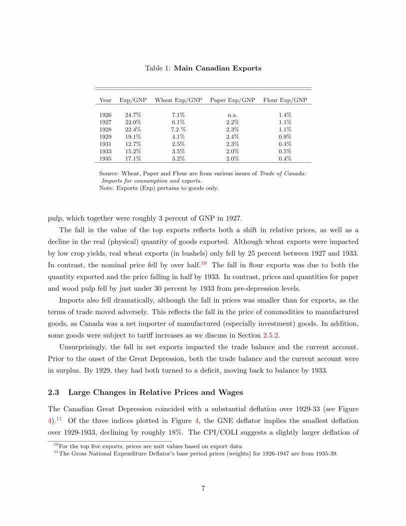
Table 1: Main Canadian Exports

Year Exp/GNP Wheat Exp/GNP Paper Exp/GNP Flour Exp/GNP

1926 24.7% 7.1% n.a. 1.4%1927 22.0% 6.1% 2.2% 1.1%1928 22.4% 7.2 % 2.3% 1.1%1929 19.1% 4.1% 2.4% 0.9%1931 12.7% 2.5% 2.3% 0.4%1933 15.2% 3.5% 2.0% 0.5%1935 17.1% 3.2% 2.0% 0.4%

Source: Wheat, Paper and Flour are from various issues of Trade of Canada:Imports for consumption and exports.

Note: Exports (Exp) pertains to goods only.

pulp, which together were roughly 3 percent of GNP in 1927.

The fall in the value of the top exports reflects both a shift in relative prices, as well as a

decline in the real (physical) quantity of goods exported. Although wheat exports were impacted

by low crop yields, real wheat exports (in bushels) only fell by 25 percent between 1927 and 1933.

In contrast, the nominal price fell by over half.10 The fall in flour exports was due to both the

quantity exported and the price falling in half by 1933. In contrast, prices and quantities for paper

and wood pulp fell by just under 30 percent by 1933 from pre-depression levels.

Imports also fell dramatically, although the fall in prices was smaller than for exports, as the

terms of trade moved adversely. This reflects the fall in the price of commodities to manufactured

goods, as Canada was a net importer of manufactured (especially investment) goods. In addition,

some goods were subject to tariff increases as we discuss in Section 2.5.2.

Unsurprisingly, the fall in net exports impacted the trade balance and the current account.

Prior to the onset of the Great Depression, both the trade balance and the current account were

in surplus. By 1929, they had both turned to a deficit, moving back to balance by 1933.

2.3 Large Changes in Relative Prices and Wages

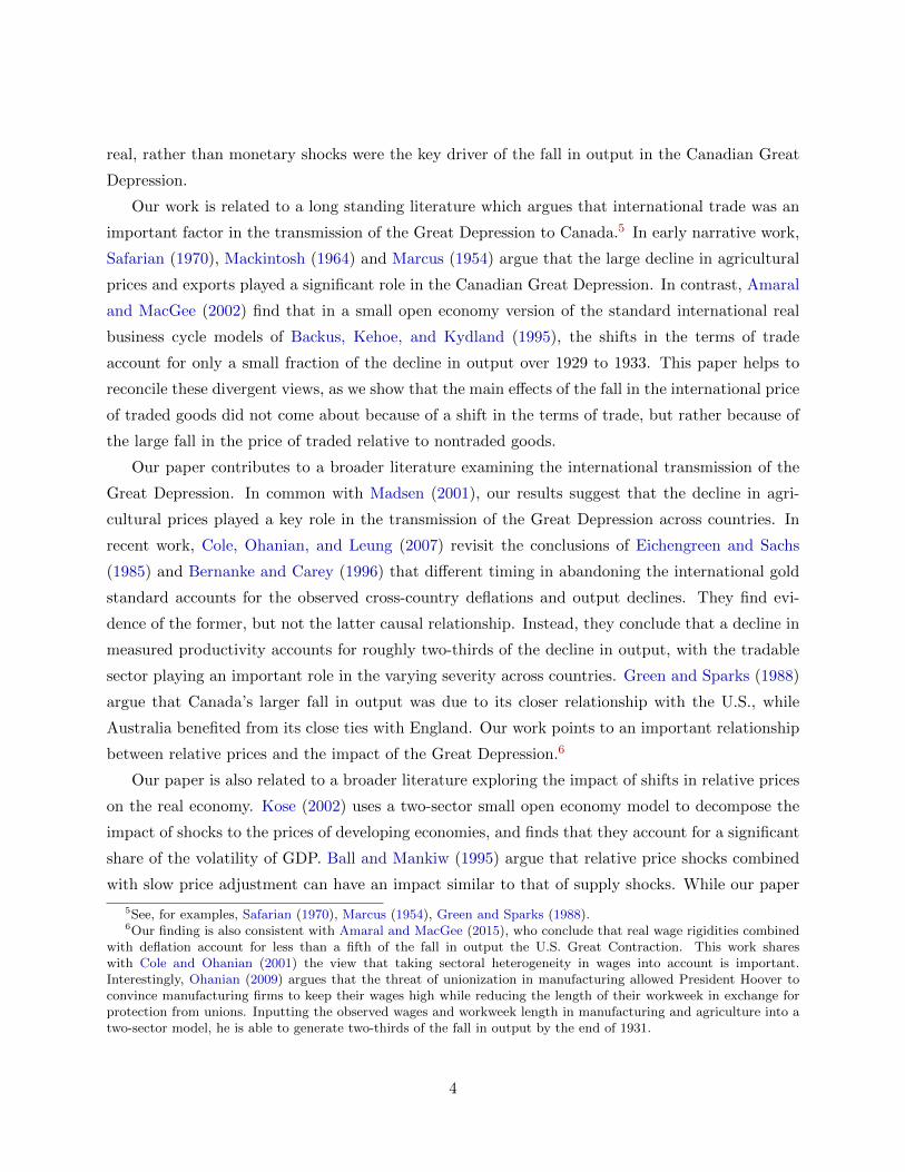
The Canadian Great Depression coincided with a substantial deflation over 1929-33 (see Figure

4).11 Of the three indices plotted in Figure 4, the GNE deflator implies the smallest deflation

over 1929-1933, declining by roughly 18%. The CPI/COLI suggests a slightly larger deflation of

10For the top five exports, prices are unit values based on export data.11The Gross National Expenditure Deflator’s base period prices (weights) for 1926-1947 are from 1935-39.

7

roughly 23 %, due to a larger decline between 1932 and 1933.12 The Wholesale Price Index (WPI)

experienced the largest decline, falling by roughly 30%.13

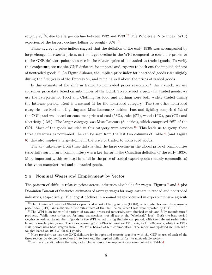
These aggregate price indices suggest that the deflation of the early 1930s was accompanied by

large changes in relative prices, as the larger decline in the WPI compared to consumer prices, or

to the GNE deflator, points to a rise in the relative price of nontraded to traded goods. To verify

this conjecture, we use the GNE deflators for imports and exports to back out the implied deflator

of nontraded goods.14 As Figure 5 shows, the implied price index for nontraded goods rises slightly

during the first years of the Depression, and remains well above the prices of traded goods.

Is this estimate of the shift in traded to nontraded prices reasonable? As a check, we use

consumer price data based on sub-indices of the COLI. To construct a proxy for traded goods, we

use the categories for Food and Clothing, as food and clothing were both widely traded during

the Interwar period. Rent is a natural fit for the nontraded category. The two other nontraded

categories are Fuel and Lighting and Miscellaneous/Sundries. Fuel and lighting comprised 6% of

the COL, and was based on consumer prices of coal (53%), coke (9%), wood (16%), gas (9%) and

electricity (13%). The larger category was Miscellaneous (Sundries), which comprised 26% of the

COL. Most of the goods included in this category were services.15 This leads us to group these

three categories as nontraded. As can be seen from the last two columns of Table 2 (and Figure

6), this also implies a large decline in the price of traded to nontraded goods.

The key take-away from these data is that the large decline in the global price of commodities

(especially agricultural commodities) was a key factor in the Canadian deflation of the early 1930s.

More importantly, this resulted in a fall in the price of traded export goods (mainly commodities)

relative to manufactured and nontraded goods.

2.4 Nominal Wages and Employment by Sector

The pattern of shifts in relative prices across industries also holds for wages. Figures 7 and 8 plot

Dominion Bureau of Statistics estimates of average wages for wage earners in traded and nontraded

industries, respectively. The largest declines in nominal wages occurred in export-intensive agricul-

12The Dominion Bureau of Statistics produced a cost of living indices (COLI), which later became the consumerprice index (CPI). We make use of the sub-indices of the COL below, since these were reported by DBS.

13The WPI is an index of the prices of raw and processed materials, semi-finished goods and fully manufacturedproducts. While most prices are for large transactions, not all are at the ”wholesale” level. Both the base periodweights as well as the number of goods in the WPI varied during the interwar period, with the different series beinglinked in overlapping years. The index spanning 1913-1925 is based on 1913 weights for 236 goods, while the 1926-1934 period uses base weights from 1926 for a basket of 502 commodities. The index was updated in 1935 withweights based on 1935-39 for 604 goods.

14More precisely, we use the GNE deflators for imports and exports together with the GDP shares of each of thethree sectors we defined in section 2.1 to back out the implied deflator for the nontradable sector.

15See the appendix where the weights for the various sub-components are summarized in Table 4.

8

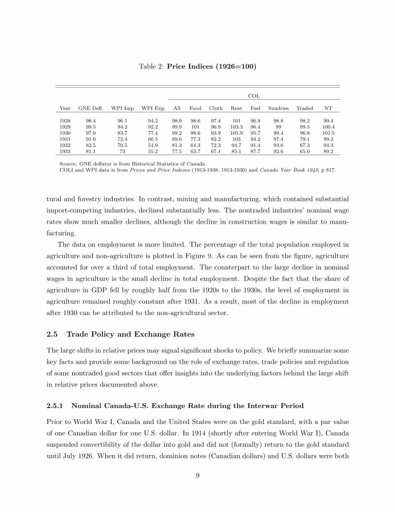
Table 2: Price Indices (1926=100)

COL

Year GNE Defl. WPI Imp WPI Exp All Food Cloth Rent Fuel Sundries Traded NT

1928 98.4 96.1 94.2 98.9 98.6 97.4 101 96.9 98.8 98.2 99.41929 99.5 94.2 92.2 99.9 101 96.9 103.3 96.4 99 99.5 100.41930 97.0 83.7 77.4 99.2 98.6 93.9 105.9 95.7 99.4 96.8 101.51931 91.0 72.4 60.5 89.6 77.3 82.2 103 94.2 97.4 79.1 99.21932 82.5 70.5 54.9 81.3 64.3 72.3 94.7 91.4 94.6 67.3 94.31933 81.1 73 55.2 77.5 63.7 67.1 85.1 87.7 92.6 65.0 89.2

Source: GNE deflator is from Historical Statistics of Canada.COLI and WPI data is from Prices and Price Indexes (1913-1938, 1913-1930) and Canada Year Book 1940, p 817.

tural and forestry industries. In contrast, mining and manufacturing, which contained substantial

import-competing industries, declined substantially less. The nontraded industries’ nominal wage

rates show much smaller declines, although the decline in construction wages is similar to manu-

facturing.

The data on employment is more limited. The percentage of the total population employed in

agriculture and non-agriculture is plotted in Figure 9. As can be seen from the figure, agriculture

accounted for over a third of total employment. The counterpart to the large decline in nominal

wages in agriculture is the small decline in total employment. Despite the fact that the share of

agriculture in GDP fell by roughly half from the 1920s to the 1930s, the level of employment in

agriculture remained roughly constant after 1931. As a result, most of the decline in employment

after 1930 can be attributed to the non-agricultural sector.

2.5 Trade Policy and Exchange Rates

The large shifts in relative prices may signal significant shocks to policy. We briefly summarize some

key facts and provide some background on the role of exchange rates, trade policies and regulation

of some nontraded good sectors that offer insights into the underlying factors behind the large shift

in relative prices documented above.

2.5.1 Nominal Canada-U.S. Exchange Rate during the Interwar Period

Prior to World War I, Canada and the United States were on the gold standard, with a par value

of one Canadian dollar for one U.S. dollar. In 1914 (shortly after entering World War I), Canada

suspended convertibility of the dollar into gold and did not (formally) return to the gold standard

until July 1926. When it did return, dominion notes (Canadian dollars) and U.S. dollars were both

9

convertible into gold at the rate of $20.67 per ounce. Although the United States also suspended

convertibility during the First World War, it returned to the gold standard in June 1919.

Figure 10 plots the Canada-U.S. nominal exchange rate, expressed as Canadian dollars per U.S.

dollar, over the 1913-1940 period. The Canadian dollar depreciated by more than 10 percent on

two occasions - once after WWI and in 1931. The depreciation of 1931 came roughly two years

after Canada de facto left the Gold Standard, as gold shipments were suspended in January 1929

(Bordo and Redish, 1990). Despite the suspension of convertibility, the Canadian government

took steps to prevent depreciation of the dollar, motivated in part by a wish to maintain access

to American capital markets to refinance Dominion debt (Shearer and Clark, 1984). As a result,

the government maintained the advance rate at its 1928 level throughout 1930, despite the fall

in world rates. This policy was ultimately abandoned after the British left the Gold Standard

in October, 1931. Subsequently, the Canadian dollar depreciated relative to the U.S. dollar by

approximately 15 percent, before beginning to appreciate after the U.S. left the Gold Standard in

March of 1933. In April of 1933, Canada “officially” confirmed the non-redemption of notes for

gold. The Canadian currency reached parity again in November 1933, although the exchange rate

fluctuated somewhat until 1935, and remained near parity until October 1939, when the Canadian

dollar again depreciated relative to the U.S. dollar.

2.5.2 Tariff and Non-Tariff Barriers

An important factor behind the shift in relative prices of export and import goods was the rise

of trade barriers in Canada and abroad. Particularly important for Canadian exports was the

dramatic rise in continental European barriers to the imports of agricultural goods (Ezekiel, 1932).

These barriers arguably helped lower the international price of Canadian agricultural exports, and

amplified the impact of the return of Russia to the world market for agricultural exports.

Although U.S. tariff policy during the Great Depression is widely discussed, the impact of

the Hawley-Smoot Tariff act of June 17, 1930 on Canada was arguably smaller than European

developments. Hawley-Smoot raised U.S. tariffs on over 20,000 imported goods, with the primary

Canadian exports affected being wheat, flaxseed, millwood, cattle, milk products, wool, and fish.16

While the U.S. was a major export destination for some of these goods (particularly live cattle),

for others, such as wheat, the U.S. market accounted for a small share of exports.

Canada also moved to increase trade barriers during the Great Depression. Canada responded

to the Hawley-Smoot act by preemptively imposing tariffs on 16 products that together accounted

for roughly 30% of U.S. exports to Canada. The main U.S. exports affected by Canadian duties

16See McDonald, O’Brien, and Callahan (1997).

10

were potatoes, eggs, fresh meats, butter, wheat, flour, and rolled oats. In addition, the Ministry of

National Revenue was provided with the authority to assign higher values to imported goods, and

fixed currency valuations were used to counteract currency dumping.17 The increase in average

tariffs from 1928 to 1933 was roughly 20 percent. Similar sized increases were put in place for

imports from the U.S. and the United Kingdom, who accounted for 68 and 15 percent of Canadian

imports in 1929, respectively.

The increases in Canadian tariffs were largely undone by 1937, as a result of trade agreements

negotiated during the 1930s. Tariffs on imports from Commonwealth countries were lowered after

1932 as a result of treaties negotiated at the Ottawa conference. In 1935, Canada and the United

States negotiated a bilateral trade agreement (the United States-Canada Trade Agreement) which

came into effect on January 1, 1936. This agreement lowered duties on roughly three-fourths of the

dutiable goods imported from the U.S. in 1929, and were significant for iron and steel products as

well as machinery (Goldenberg, 1936).18

2.5.3 Regulation: A Partial Explanation for the Small Decline in Nontraded Prices

While the fall in traded goods’ prices reflected global market trends, nontraded prices were deter-

mined endogenously. This raises the question of what frictions could be responsible for the small

decline in nontraded prices during the Great Depression.

A partial explanation for this slow adjustment is government regulation. Although Amaral and

MacGee (2002) document that there was no NRA-type intervention by Canadian governments,

nontraded transportation industries were subject to price regulation in Canada, both directly and

indirectly via government ownership. These industries accounted for 10− 13% of nominal GDP in

Canada (and the United States), or roughly a fifth of the nontraded sector. This regulation involved

all three levels of government. For example, city tramlines were often directly or indirectly regulated

by municipal governments.19 Public utilities and railway prices were also regulated in both Canada

and the United States, and these prices were not adjusted downwards during the Great Depression.

Public utilities such as power companies and local railways were regulated by Provincial bodies

during the interwar period in Canada (Currie, 1946). Although little academic work has explored

the behavior of Canadian utilities during this period, Sumner (1939) documents that the prices of

a variety of public and utility goods did not decline (and in several cases increased) during the U.S.

Great Depression. O’Brien (1989) argues that the Interstate Commerce Commission’s regulation

17See McDiarmid (1947) and Brecher (1957). These tariffs had differential impacts across provinces. MacGregor(1935) outlines the practical challenges with quantifying these differential impacts, although the agreed view is thattariffs tended to boost the prices of manufacturing firms mainly located in Ontario and Quebec.

18Tariffs on fish, cattle, lumber, cheese, cream, whiskey and potatoes were also reduced.19See Thurston (1938) for a discussion of the Toronto Transportation Commission and prices.

11

of prices meant that freight rates not only did not fall, but actually increased during the 1930s.

Canada also had a commission which regulated freight rates, and for many of the most important

routes, the rates were set to correspond to U.S. railway rates.

This evidence points to a role for government in the slow decline of nontraded prices. However,

it leaves open why other nontraded prices also seemed to adjust slowly, as indicated by the small

decline in the Sundries index of the COLI in Table 2.

2.6 Agricultural Yields in Field Crops

The agricultural sector played a large role in the Canadian interwar economy, and accounted for over

18 percent of GDP at factor cost in 1926, whereas by the mid-2000s agriculture accounted for less

than 2 percent. This large role is relevant for our work for two reasons. First, as discussed above,

this meant that the large swings in international prices of agricultural goods significantly impacted

the real income of Canadians. Second, the large agricultural sector left the Canadian economy more

exposed to adverse weather shocks than today. The Canadian prairie provinces were particularly

affected by a severe drought that began in 1929 and continued, with some respites, until midsummer

of 1937 (Marchildon, Kulshreshtha, Wheaton, and Sauchyn, 2008).

To examine the potential impact of adverse weather, we look at crop yields for the main field

crops.20 Yields are defined as total output of a specific crop (e.g., bushels of wheat) divided by

cultivated acreage. To measure the impact of variations in weather conditions, we look at the yield

relative to the average yield for major field crops over 1920-1940. To construct an average yield

for all field crops, we use as weights the ratio of each crop’s farm gross value of production to total

farm gross value for field crops.21

Figure 18 plots the annual yield relative to the mean yield for our major field crops average as

well as for Wheat and Oats, which were the two most important field crops, accounting for nearly

eighty percent of farm gross value in 1926. There are two key points to take from the plot. First,

yields during most of the 1930s were below the 1920s. Although the lowest yields coincide with

the worst of the Dust Bowl during the mid to late 1930s, crop yields were also low in 1929, 1931

and 1933. In contrast, 1928 (when GDP peaks prior to the Canadian Depression) was a year of

exceptionally high yields. Second, the variations in average yields were large, varying from peaks

of nearly 40 percent above the average in 1928 to nearly 40 percent below in 1937. The variation

in wheat yields was even larger, as variation in yields for other field crops tended to be less than

that of wheat.

20The data is from Historical Statistics of Canada Series M249-300.21We include all field crops with at least five hundred thousand dollars worth of gross farm revenue in 1926. This

includes wheat, oats, barley, mixed grains, corn, buckwheat and potatoes.

12

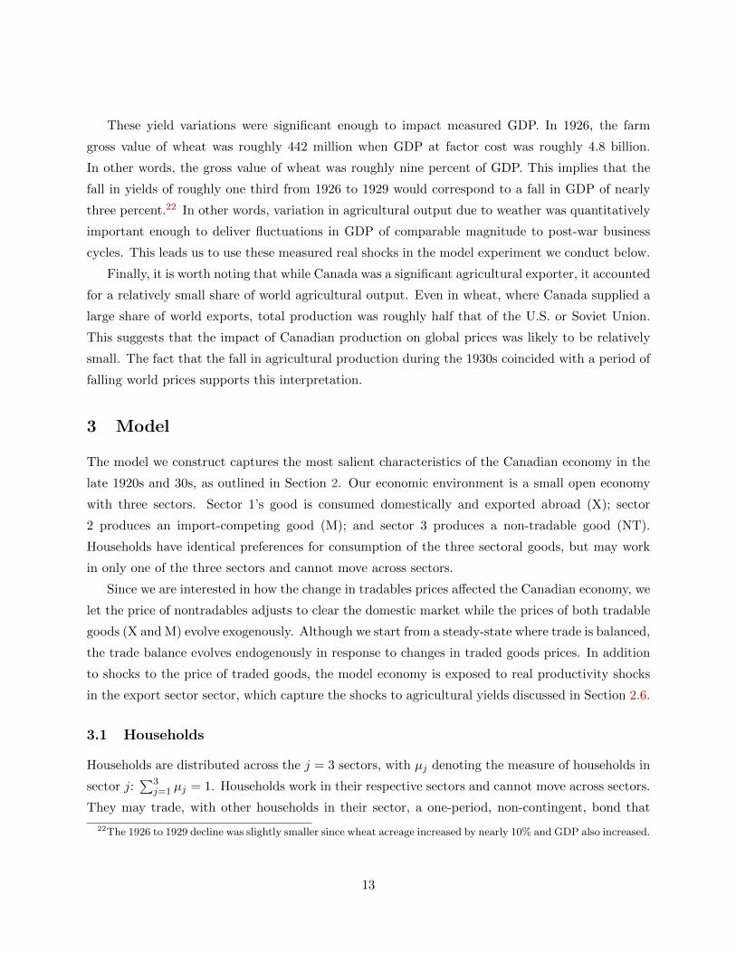
These yield variations were significant enough to impact measured GDP. In 1926, the farm

gross value of wheat was roughly 442 million when GDP at factor cost was roughly 4.8 billion.

In other words, the gross value of wheat was roughly nine percent of GDP. This implies that the

fall in yields of roughly one third from 1926 to 1929 would correspond to a fall in GDP of nearly

three percent.22 In other words, variation in agricultural output due to weather was quantitatively

important enough to deliver fluctuations in GDP of comparable magnitude to post-war business

cycles. This leads us to use these measured real shocks in the model experiment we conduct below.

Finally, it is worth noting that while Canada was a significant agricultural exporter, it accounted

for a relatively small share of world agricultural output. Even in wheat, where Canada supplied a

large share of world exports, total production was roughly half that of the U.S. or Soviet Union.

This suggests that the impact of Canadian production on global prices was likely to be relatively

small. The fact that the fall in agricultural production during the 1930s coincided with a period of

falling world prices supports this interpretation.

3 Model

The model we construct captures the most salient characteristics of the Canadian economy in the

late 1920s and 30s, as outlined in Section 2. Our economic environment is a small open economy

with three sectors. Sector 1’s good is consumed domestically and exported abroad (X); sector

2 produces an import-competing good (M); and sector 3 produces a non-tradable good (NT).

Households have identical preferences for consumption of the three sectoral goods, but may work

in only one of the three sectors and cannot move across sectors.

Since we are interested in how the change in tradables prices affected the Canadian economy, we

let the price of nontradables adjusts to clear the domestic market while the prices of both tradable

goods (X and M) evolve exogenously. Although we start from a steady-state where trade is balanced,

the trade balance evolves endogenously in response to changes in traded goods prices. In addition

to shocks to the price of traded goods, the model economy is exposed to real productivity shocks

in the export sector sector, which capture the shocks to agricultural yields discussed in Section 2.6.

3.1 Households

Households are distributed across the j = 3 sectors, with µj denoting the measure of households in

sector j:∑3

j=1 µj = 1. Households work in their respective sectors and cannot move across sectors.

They may trade, with other households in their sector, a one-period, non-contingent, bond that

22The 1926 to 1929 decline was slightly smaller since wheat acreage increased by nearly 10% and GDP also increased.

13

pays interest rate Rjt.

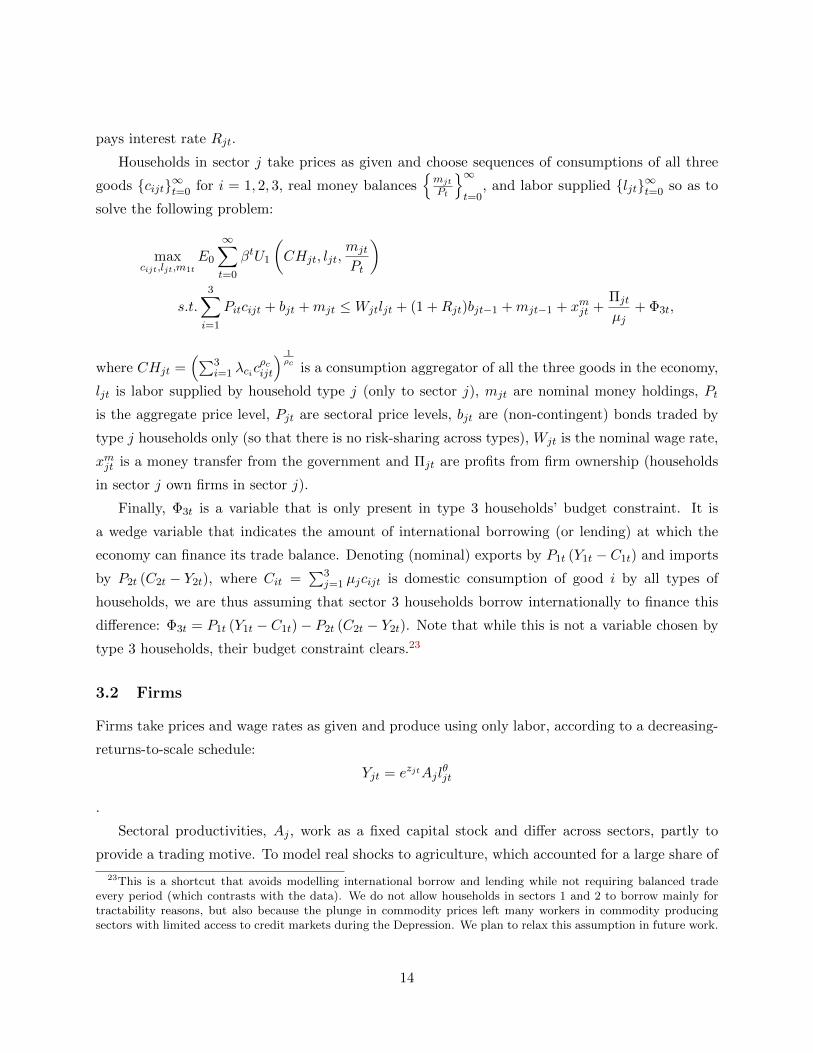
Households in sector j take prices as given and choose sequences of consumptions of all three

goods {cijt}∞t=0 for i = 1, 2, 3, real money balances{mjtPt

}∞t=0

, and labor supplied {ljt}∞t=0 so as to

solve the following problem:

maxcijt,ljt,m1t

E0

∞∑t=0

βtU1

(CHjt, ljt,

mjt

Pt

)

s.t.

3∑i=1

Pitcijt + bjt +mjt ≤Wjtljt + (1 +Rjt)bjt−1 +mjt−1 + xmjt +Πjt

µj+ Φ3t,

where CHjt =(∑3

i=1 λcicρcijt

) 1ρc is a consumption aggregator of all the three goods in the economy,

ljt is labor supplied by household type j (only to sector j), mjt are nominal money holdings, Pt

is the aggregate price level, Pjt are sectoral price levels, bjt are (non-contingent) bonds traded by

type j households only (so that there is no risk-sharing across types), Wjt is the nominal wage rate,

xmjt is a money transfer from the government and Πjt are profits from firm ownership (households

in sector j own firms in sector j).

Finally, Φ3t is a variable that is only present in type 3 households’ budget constraint. It is

a wedge variable that indicates the amount of international borrowing (or lending) at which the

economy can finance its trade balance. Denoting (nominal) exports by P1t (Y1t − C1t) and imports

by P2t (C2t − Y2t), where Cit =∑3

j=1 µjcijt is domestic consumption of good i by all types of

households, we are thus assuming that sector 3 households borrow internationally to finance this

difference: Φ3t = P1t (Y1t − C1t)− P2t (C2t − Y2t). Note that while this is not a variable chosen by

type 3 households, their budget constraint clears.23

3.2 Firms

Firms take prices and wage rates as given and produce using only labor, according to a decreasing-

returns-to-scale schedule:

Yjt = ezjtAjlθjt

.

Sectoral productivities, Aj , work as a fixed capital stock and differ across sectors, partly to

provide a trading motive. To model real shocks to agriculture, which accounted for a large share of

23This is a shortcut that avoids modelling international borrow and lending while not requiring balanced tradeevery period (which contrasts with the data). We do not allow households in sectors 1 and 2 to borrow mainly fortractability reasons, but also because the plunge in commodity prices left many workers in commodity producingsectors with limited access to credit markets during the Depression. We plan to relax this assumption in future work.

14

the export sector, we allow for productivity shocks in sector X. This means that z2t = z3t = 0 for

all t, while we model the evolution of this process in sector X as an AR(1): z1t+1 = ρzz1t + εzt+1,

where the innovations are iid εzt+1 ∼ N(0, σ2z).

Although firms in sectors j = 1, 2 take prices P1t, P2t as given, since goods 1 and 2 are traded,

domestic consumption need not equal domestic production at that given (world) price. In fact,

our calibration guarantees that production of sector X goods exceeds domestic consumption (real

exports equal Y1t−C1t) and vice-versa for sector M (real imports equal C2t−Y2t). In the NT sector

the price level, P3t adjusts so that the product market clears (Y3t = C3t) for every period t.

3.3 Money

Money is supplied exogenously by the government through transfers to households. Its period

budget constraint is Mt −Mt−1 = Xt, where Xt =∑3

j=1 µjxmjt and money market clearing yields

Mt =∑3

j=1 µjmjt. The growth rate of the stock of money, gt = logMt − logMt−1 follows an

exogenous AR(1) process: gt+1 = g+ρmgt+εmt+1, where the innovations are iid εmt+1 ∼ N(0, σ2m).

Since the stock of money is growing, nominal variables in the model are not stationary. We

render them stationary by dividing by the stock of money. To that end define Pjt =PjtMt

, bjt =bjtMt

,

Pt = PtMt

, Wjt =Wjt

Mt, xmjt =

xmjtMt

Φ3t = Φ3tMt

Πjt =ΠjtMt

, and Xt = XtMt

.

Prices in the traded sectors (j = 1, 2) also evolve exogenously. We start by rendering prices

stationary by dividing them by the money supply: Pjt =PjtMt

. We then assume that the stationary

price level’s law of motion is given by an AR(1): Pjt+1 = pj +ρpj Pjt+εpjt+1 , where the innovations

are iid εpjt+1 ∼ N(0, σ2pj ).

Given g0, M0, and the laws of motion for the stock of money and prices in the traded sectors, an

equilibrium is quantities{bjt, cjt, cijt, Cjt, Yjt, ljt, Xt, x

mjt , Φ3t, Πjt

}∞t=0

, for i = 1, 2, 3 and j=1, 2, 3

and prices{P3t, Pt, Rjt, Wjt, xjt

}∞t=0

, for j = 1, 2, 3, such that all households and firms in each

sector solve the problems described above subject to market clearing conditions. The households’

and firms’ first-order conditions, together with the wage setting equations and the market clearing

conditions for the sectoral goods and for the labor market in the export sector constitute the set

of necessary conditions for an equilibrium.

3.4 Parameterization

We parameterize the model economy to match key moments of the Canadian economy in 1926,

prior to the decline in the prices of tradable goods. We set the model period to equal one year,

since most of the available macro data for Canada is annual.

Our data counterpart of the export sector is the sum of Agriculture, Forests and Fishing, Mining,

15

and three manufacturing industries: Food, Wood, and Pulp and Paper. The importin-competing

sector is the remainder of Manufacturing, while the nontraded sector is the rest of the economy.

This repartition implies that in steady-state, the export sector (X) accounts for 33 percent of GDP,

while the import competing sector (M) accounts for 12 percent. In terms of employment, sector X

accounts for 45 percent while sector M is responsible for 12 percent. We also constrain the model

parameters such that the value-added share of imports (and exports, given our balanced-trade

assumption) is 29 percent in steady-state. This gives us five moments to target.

The momentary utility form is additive in consumption, labor and real money balances:

U1

(CH1t, l1t,

m1t

Pt

)=CH1−σ

1t

1− σ− l1−σL1t

1− σL+ λM

(m1tPt

)1−σM

1− σM

We make the following normalizations:∑3

i=1 λci = 1 and A3 = 1. We let preferences be

logarithmic in aggregate consumption (σ = 1). We set the elasticity of substitution between

the different consumption goods to two-thirds (ρc = −0.5) and the Frisch elasticity to one-half

(σL = −2), values that are common in the literature. We also opt for log preferences in real

money balances (σm = 1) so as to have a unit elasticity with respect to consumption. We perform

sensitivity analysis with respect to the utility curvature parameters below.

We estimate an AR(1) process for the growth rate of money on yearly M1 data from 1921 to

1971. This yields g = 0.0161, ρm = 0.6509 and σg = 0.05. This implies a steady-state money

growth rate of gm = g1−ρ = 0.0461. Given a model period of one year, targeting a nominal interest

rate of 5.6 percent implies β = 1+gm1+R ' 0.99.24 All parameter values are summarized in Table 3.

3.5 Shocks

Our benchmark experiment consists of feeding in two sets of shocks: (1) a sequence of esti-

mated price shock innovations {εp1t , εp2t}1939t=1926 constructed to match the path of tradables’ prices

{P1t, P2t}1939t=1926; and (2) a sequence of estimated real productivity shock innovations to sector X,

{εzt}1939t=1926.

We use the GNE deflator series for exports and imports as the data targets for our prices (see

Figure 5). We stationarize the price series {P1t, P2t}1939t=1926 by dividing by their 1926-70 growth rate.

We then estimate AR(1) processes for both series. We obtain ρp1 = 0.9676, ρp2 = 0.9586. Using

this, we back out the residuals, {εp1t , εp2t}1939t=1926, that yield the observed price paths in the model

and in the data.

24The nominal interest rate on long-term dominion bonds averaged 5.6 percent in the 1920s. We could not finddata on shorter maturity government bonds.

16

To obtain a series of real shocks in sector X, {z1t}1939t=1926, we use the data on real yields described

in Section 2.6 (see Figure 18). We estimate an AR(1) on the stationarized average yields series and

then rescale the variance of the shocks to reflect the fact that agriculture was roughly 55 percent of

the X sector in value added terms and that field crops represented about two-thirds of agricultural

gross revenues in 1926. From this estimation we obtain ρz = 0.52 and σz = 0.07.

4 Results

Our counterfactual experiments quantify the contribution of shocks to traded goods prices and

variations in agricultural yields to the fall in output during the Canadian Great Depression. We

first examine these shocks using a version of the model without nominal frictions. We find that the

fall in the price of tradables over 1928 to 1933 has little impact on output as the nontradable price

falls nearly as much. As a result, the model does not generate the rise in the price of nontraded

goods relative to traded goods observed in the data.

This leads us to introduce nominal frictions to generate a shift in relative prices in response to

the fall in traded goods prices. Since the contraction period was characterized by increases in real

wages in sectors M and NT, as shown in Figure 11, we opt for modeling nominal wage frictions by

assuming that in these two sectors, nominal wages are determined by Taylor-type wage contracts.25

The fall in tradables prices interacts with these frictions along two key margins. First, the

increase in sector M’s real product wage results in a substantial fall in production. This fall is

even larger than in a closed economy model, since households can import relatively cheap sector M

goods. In the NT sector prices cannot go down as much as in the frictionless environment because

this implies an increase in real wages, given the nominal wage sluggishness. As a result, the relative

price of nontradables to tradables goes up just like in the data, and the production in the NT sector

is reduced. When we add to this the impact of the real shocks to the exporting sector, we obtain

a fall in aggregate output that is over half of what we see in the data.

4.1 No Nominal Frictions

In Amaral and MacGee (2002), we found that terms of trade shocks in a frictionless small open

economy (as in Backus, Kehoe, and Kydland (1995)) calibrated to the interwar Canadian economy

imply a small decline in aggregate output. We find a similar result here in our nominal multi-sector,

frictionless, environment when we feed in the computed price shocks.26

25Figure 11 shows industry nominal wages deflated by the sectoral price. Thus, while Manufacturing is deflated bythe import price, the service wages are deflated by our computed nontraded price.

26We focus on the price shocks only here since this motivates the extension of the model to include nominalrigidities. Including the real shocks to sector X in the frictionless version of our model economy does not change the

17

The impact of the fall in the prices of traded goods on real output is small, peaking at 3 percent

(see Figure 13). This is mainly due to the fall in nontraded price and wages that nearly parallel

the fall in tradable prices and wages. As a result, real product wages remain nearly constant in all

three sectors. Since real wages fail to move significantly, neither does labor, or output.

This downward adjustment of nominal wages to the fall in prices corresponds to what is observed

in the data for agriculture and logging (see Figure 7). However, it contrasts with what happened

in manufacturing or in some of the services (see Figure 8). There, real wages increased, sometimes

substantially, as Figure 11 shows. This leads us to introduce staggered wage contracts in our model

economy in the following section.

4.2 Nominal wage frictions

We extend our model and assume that wages in sectors 2 and 3 adjust slowly due to nominal

rigidities and that hours are determined by the short side of the market in these sectors. This

means that firms optimally set hours according to their marginal product of labor schedule in

sectors M and NT. While the firms do not have to necessarily be the short side of the market, in

this case, because of the high real wages, the hours the households want to supply will turn out to

be be higher than those that firms wish to employ given the path of prices.27 In sector 1, the wage

rate adjusts to clear the market (i.e., labour demand is equated to labour supplied).

In the M and NT sectors, wages are subject to Taylor-type contracts. Labor is divided into two

equally-sized cohorts and each period, the contract wage of one of the cohorts is adjusted. The

nominal wage the firm pays is a geometric average of the two cohorts’ contract wages:

Wjt = x0.5jt x

0.5jt−1, j = 2, 3. (1)

The contract wage in period t, xjt, depends on the current and future expected nominal wages

and labor gaps relative to steady-state, so that:

log xjt = 0.5 logWjt + γj(Ljt − Lj

)+ Et

{0.5 logWjt+1 + γ

(Ljt+1 − Lj

)}j = 2, 3. (2)

where γj is a labor-gap adjustment parameter.

Repeated substitution of (1) into (2) yields the current contract wage as a function of past and

message that the model is unable to generate the shift in the relative price of traded to nontraded goods observed inthe data.

27We verify ex-post that indeed, the hours that come out of the households’ FOC given the wage rate are higherthan those that come out of the firms’ FOC in sectors 2 and 3 for all the periods in our experiment.

18

expected contract wages and the current and expected labor gaps:

log xjt =1

2log xjt−1 + 2γj

(Ljt − Lj

)+ Et

{1

2log xjt+1 + 2γj

(Ljt+1 − Lj

)}.

A crucial parameter is γj , which controls the degree of nominal wage adjustment, as per equation

2. To discipline this parameter, we pick values for γj such that the sectoral real product wages

the model generates increase as much as in the data up until 1933. Figure 11 shows real wages for

selected industries (deflated by the respective sectoral price). The manufacturing real wage had

increased roughly 30 percent by 1933, so we set γ2 so that the real wage in the import-competing

sector in the model increases by 30 percent also. The increase in real wages for services was lower,

as the real wages for Construction, Telephone and Rail in the same figure illustrate. Accordingly,

we (conservatively) set γ3 so that the real wage in the model’s NT sector increases by 6 percent.

In our our benchmark experiment we input the price shocks and the real shocks to sector X. As

panel A in Figure 15 shows, the combination of price shocks, TFP shocks, and nominal frictions

implies a decline in real output of 17 percent at the trough: over half of the fall seen in the data.

In sector X, the fall in model output is about a third of that in the data and it is entirely driven

by the real agricultural shocks, since X-sector hours are constant (panel B of Figure 17). This is

due to our log specification in the consumption aggregate, which implies the income effect and the

substitution effect from a change in the real wage cancel out. This does not happen for the two

other sectors since the firm side determines hours there.

In the nontraded sector, the fall in output is over half that in the data, as seen in panel D of

Figure 15. While the model overstates the fall in output in the import-competing sector (panel C),

this overprediction does not drive the fall in aggregate output since the share of sector M in GNP

is only 12 percent. It is instead because the nominal wage friction is preventing the NT price from

adjusting down in line with the tradables prices.

While, by construction, we match the fall in prices in the two tradable sectors, as panels B and

C of Figure 16 show, the model does a good job of keeping the NT price from falling too much

(panel D). Consequently it matches the aggregate price quite well (panel A). Absent the nominal

frictions in sector NT, prices in this sector would fall roughly in line with tradables prices. A

smaller nominal wage friction in sector NT would allow the NT price to adjust downward toward

the data, but the increase in the real product wage rate would then be smaller, and less in line with

the data, also implying less downward action in NT (and aggregate) output.

The fact that the model generates no fall in hours in sector X implies that on aggregate, the

fall in hours is smaller than in the data, as panel A in Figure 17 shows, despite the fact that hours

19

in sector M fall much more than in the data (panel C).28 Nonetheless, the model does a good job of

matching the fraction of the output fall that changes in total hours are responsible for. Measuring

aggregate total factor productivity (TFP) simply by YtLθt

, Figure 19 shows that the model captures

half of the fall in TFP from 1926 to 1933 but misses the run-up to 1929. Most of this initial increase

in measured TFP is coming from sector M, where we do not model real shocks. Sector M’s output

per capita increased by roughly 30 percent from 1926 to 1929, while hours only increased by 10

percent.

Regarding foreign trade, we are assuming the economy starts out from balanced-trade where

exports and imports both account for 29 percent of GDP. From there, both nominal imports and

exports fall: by 10 percent and 44 percent at the trough, respectively. Together with the fall in

GDP this implies a trade deficit at the trough of roughly 13 percent of GDP, somewhat larger than

the fall we see in the data, as Figure 20 shows.

Real consumption decreases the most for households in sector M, even as their real consumption

wage goes up by 12 percent. This is because their real compensation goes down by roughly 50

percent, as their labor plummets, as shown in panel C of Figure 17. The fact that they continue

to supply the same amount of labor does not prevent consumption for households in sector X from

declining roughly 25 percent, as their nominal wage falls by 35 percent, roughly in line with the

fall in the price of exports. Finally, households in the NT sector actually experience a purchasing

power increase.29

The relative role of individual shocks

To asses the relative importance of the two kinds of exogenous shocks in our model we run

two experiments where we subject our model economy to one set of shocks at the time. Figure

21 indicates that the price shocks play the more prominent role, but real technological shocks are

instrumental in generating a hump in the early years, as well as in delivering the trough in 1933 as

opposed to 1932, which is what happens when only price shocks operate.

The relative role of individual frictions

The main driver of the fall in output are the nominal wage frictions in sectors M and NT. To

better understand their individual role, we run two experiments where we turn off these frictions

one at a time and let the wage in the respective sector move such as to clear the labor market at

28Again, recall that because of sector M’s small size, the quantitative impact of this overprediction is small.29This increase happens because sector NT households are allowed to borrow internationally to finance the trade

deficit, while not internalizing the cost of those loans, as detailed in section 3.1. Were sector 3 households to decideoptimally on the amount they borrow internationally, we conjecture their consumption would be lower and the fallin aggregate output would be even larger.

20

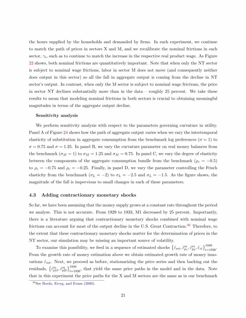
the hours supplied by the households and demanded by firms. In each experiment, we continue

to match the path of prices in sectors X and M, and we recalibrate the nominal frictions in each

sector, γi, such as to continue to match the increase in the respective real product wage. As Figure

22 shows, both nominal frictions are quantitatively important. Note that when only the NT sector

is subject to nominal wage frictions, labor in sector M does not move (and consequently neither

does output in this sector) so all the fall in aggregate output is coming from the decline in NT

sector’s output. In contrast, when only the M sector is subject to nominal wage frictions, the price

in sector NT declines substantially more than in the data – roughly 25 percent. We take these

results to mean that modeling nominal frictions in both sectors is crucial to obtaining meaningful

magnitudes in terms of the aggregate output decline.

Sensitivity analysis

We perform sensitivity analysis with respect to the parameters governing curvature in utility.

Panel A of Figure 24 shows how the path of aggregate output varies when we vary the intertemporal

elasticity of substitution in aggregate consumption from the benchmark log preferences (σ = 1) to

σ = 0.75 and σ = 1.25. In panel B, we vary the curvature parameter on real money balances from

the benchmark (σM = 1) to σM = 1.25 and σM = 0.75. In panel C, we vary the degree of elasticity

between the components of the aggregate consumption bundle from the benchmark (ρc = −0.5)

to ρc = −0.75 and ρc = −0.25. Finally, in panel D, we vary the parameter controlling the Frisch

elasticity from the benchmark (σL = −2) to σL = −2.5 and σL = −1.5. As the figure shows, the

magnitude of the fall is impervious to small changes in each of these parameters.

4.3 Adding contractionary monetary shocks

So far, we have been assuming that the money supply grows at a constant rate throughout the period

we analyse. This is not accurate. From 1929 to 1933, M1 decreased by 25 percent. Importantly,

there is a literature arguing that contractionary monetary shocks combined with nominal wage

frictions can account for most of the output decline in the U.S. Great Contraction.30 Therefore, to

the extent that these contractionary monetary shocks matter for the determination of prices in the

NT sector, our simulation may be missing an important source of volatility.

To examine this possibility, we feed in a sequence of estimated shocks{εmt, ε

mp1 , ε

mp2 , εzt

}1939

t=1926.

From the growth rate of money estimation above we obtain estimated growth rate of money inno-

vations εmt. Next, we proceed as before, stationarizing the price series and then backing out the

residuals,{εmp1t, ε

mp2t

}1939

t=1926, that yield the same price paths in the model and in the data. Note

that in this experiment the price paths for the X and M sectors are the same as in our benchmark

30See Bordo, Erceg, and Evans (2000).

21

(and in the data). It is the estimated price innovations that are different. Again, we re-estimate

the parameters regulating the degree of nominal wage frictions, γi, so as to continue to hit the same

targets as before. As Figure 23 shows, modeling contractionary monetary shocks adds little to the

model’s ability to match the fall in output.

Nonetheless, one should not be quick to dismiss deflationary shocks as an important factor in the

downturn just because of this result. Unlike what happened in the U.S., where the monetary base

was controlled by the Federal Reserve, in Canada this was not the case, which implies that making

inference about the importance of deflationary shocks by modeling changes in M1’s growth rate as an

exogenous process may not be warranted. Note, in particular that the model endogenously delivers

a very realistic deflation simply through the combination of the Canadian’s economy exposure to

the collapse in tradable prices and the presence of domestic nominal wage frictions.

5 Conclusion

We argue that changes in relative prices are important in accounting for the decline in Canadian

output in the Great Depression. The price of tradables fell substantially, relative to that of non-

tradables, in Canada after 1926. Price shocks designed to mimic these price changes, together

with real shocks to the export sector, that are intended to stand in for weather shocks the (large)

Canadian agricultural sector suffered through the Dust Bowl years, interact with wage rigidities in

the import-competing and nontraded sectors of our multi-sector model economy to generate a fall

in real output that is over half the one seen in the data.

The large fall in the relative price of tradables to non-tradables during the Great Depression

had hitherto been a fact that, while not entirely ignored, did not merit much consideration as

a possible factor behind the large output collapses. Our research points to this being a serious

possibility, especially for small open economies that largely relied on commodity exports at the

time, like Canada, but also like Australia and Argentina. Moreover, while surely smaller in relative

scale, it would be interesting to see what the implications are for the U.S. economy.

Although our model economy captures key features of the interwar Canadian economy, it ab-

stracts from some potentially important features such as capital accumulation and international

borrowing and lending. We plan to explore these mechanisms in future work.

22

References

Amaral, P., and J. MacGee (2002): “The Great Depression in Canada and the United States:

A Neoclassical Perspective,” Review of Economic Dynamics, pp. 659–84.

(2015): “Re-Examining the Role of Sticky Wages in the U.S. Great Contraction: A

Multi-Sector Approach,” EPRI Working Paper 2012-5.

Backus, D., P. Kehoe, and F. Kydland (1995): “International Business Cycles: Theory and

Evidence,” in Frontiers of Business Cycle Research, ed. by T. F. Cooley, pp. 331–356. Princeton

University Press.

Ball, L., and G. Mankiw (1995): “Relative-Price Changes as Aggregate Supply Shocks,” Quar-

terly Journal of Economics, 110(1), 161–193.

Bernanke, B. S., and K. Carey (1996): “Nominal Wage Stickiness and Aggregate Suply in the

Great Depression,” Quarterly Journal of Economics, III(3), 853–858.

Betts, C., M. Bordo, and A. Redish (1996): “A Small Open Economy in Depression: Lessons

From Canada in the 1930s,” The Canadian Journal of Economics, 29(1), 1–36.

Bordo, M., and A. Redish (1990): “Credible Commitment and Exchange Rate Stability:

Canada’s Interwar Experience,” Canadian Journal of Economics, 23(2), 1–24.

Bordo, M. D., C. J. Erceg, and C. L. Evans (2000): “Money, Sticky Wages, and the Great

Depression,” The American Economic Review, 90(5), 1447–1453.

Brecher, I. (1957): Monetary and Fiscal Thought and Policy in Canadea: 1919-1939. University

of Toronto Press, Toronto.

Cole, H. L., and L. E. Ohanian (2001): “Re-examining the Contributions of Money and

Banking Shocks to the U.S. Great Depression,” in NBER Macroeconomics Annual 2000, ed.

by B. Bernanke, and K. Rogoff, pp. 183–227. MIT Press, Cambridge, MA.

(2004): “New Deal Policies and the Persistence of the Great Depression: A General

Equilibrium Analysis,” Journal of Political Economy, 112(4), 789–816.

Cole, H. L., L. E. Ohanian, and R. Leung (2007): “The International Great Depression:

Deflation, Productivity and the Great Depression,” mimeo.

Currie, A. (1946): “Rate Control on Canadian Public Utilities,” Canadian Journal of Economics

and Political Science, 12(2), 148–158.

23

Dominion Bureau of Statistics (1930): The Canada Year Book 1930Ottawa, Ontario.

Eichengreen, B. (1992): “The Origens and Nature of the Great Slump Revisited,” The Economic

History Review, 45(2), 213–239.

(1995): Golden Fetters: The Gold Standard and the Great Depression 1919-1939. Oxford

University Press, New York.

Eichengreen, B., and J. Sachs (1985): “Exchange Rates and Economic Recovery in the 1930s,”

Journal of Economic History, XLV, 925–946.

Ezekiel, M. (1932): “European Competition in Agricultural Production, with Special Reference

to Russia,” Journal of Farm Economics, 14(2), 267–281.

Goldenberg, H. C. (1936): “The Canada-United States Trade Agreement, 1933,” Canadian

Journal of Economics and Political Science, 2(2), 209–212.

Green, A. G., and G. R. Sparks (1988): A Macro Interpretation of Recovery: Australia and

Canadavol. Recovery from the Depression: Australia and the World Economy in the 1930s, pp.

89–112. Cambridge University Press.

Haubrich, J. (1990): “Nonmonetary Effects of Financial Crisis: Lessons from the Great Depres-

sion in Canada,” Journal of Monetary Economics, 25, 223–252.

Kose, A. (2002): “Explaining business cycles in small open economies: ’How much do world prices

matter?’,” Journal of International Economics, 56, 299–327.

Lewis, W. A. (1949): Economic Survey: 1919-1939. Unwin University Books, London.

MacGregor, D. (1935): “The Provincial Incidence of the Canadian Tariff,” Canadian Journal

of Economics and Political Science, 1(3), 384–395.

Mackintosh, W. (1964): The Economic Background of Dominion-Provincial Relations: Appendix

III of the Royal Commission Report on Dominion-Provincial Relations, Carleton Library No. 13.

McClelland and Stewart, Toronto.

Madsen, J. B. (2001): “Agricultural Crises and the International Transmission of the Great

Depression,” The Journal of Economc History, 61(2), 327–365.

Marchildon, G., S. Kulshreshtha, E. Wheaton, and D. Sauchyn (2008): “Drought and

Institutional Adaption in the Great Plains of Alberta and Saskatchewan, 1914-1939,” Natural

Hazards, (45), 391–411.

24

Marcus, E. (1954): Canada and the International Business Cycle, 1927-1939. University of

Toronto Press, Toronto.

McDiarmid, O. (1947): “Canadian Tariff Policy,” Annals of the American Acadamy of Political

and Social Science, 253, 150–157.

McDonald, J. A., A. P. O’Brien, and C. M. Callahan (1997): “Trade Wars: Canada’s

Reaction to the Smoot-Hawley Tariff,” Journal of Economic History, 57, 802–826.

O’Brien, A. P. (1989): “The ICC, Freight Rates, and the Great Depression,” Explorations in

Economic History, 26, 73–98.

Ohanian, L. E. (2009): “What - or who - started the Great Depression?,” Journal of Economic

Theory, 144, 2310–2335.

Safarian, A. (1970): The Canadian Economy in the Great Depression. McLelland and Stewart,

Toronto.

Shearer, R., and C. Clark (1984): in A Retrospective on the Classical Gold Standard, ed. by

M. Bordo, and A. Schwartzchap. Canada and the Interwar Gold Standard, 1920-35: Monetary

Policy without a Central Bank, pp. 277–310. University of Chicago Press, Chicago.

Sumner, J. D. (1939): “Public Utility Prices and the Business Cycle: A Study in the Theory of

Price Rigidity,” The Review of Economics and Statistics, 21(3), 97–109.

Temin, P. (1993): “Transmission of the Great Depression,” Journal of Economic Perspectives,

7(2), 87–102.

Thurston, J. (1938): “The Toronto Transportation Commission,” Journal of Land & Public

Utility Economics, 14(1), 10–18.

25

Table 3: Parametrization

Parameter Value Target

β 0.99 Annual nominal interest rate 5.6%γ2 0.004 Match increase in M real wageγ3 0.001 Match increase in NT real wageµ1 0.45 Employment in sector X: 45%µ2 0.12 Employment in sector M: 12%λc1 0.013 GDP share of sector X: 33%λc2 0.454 GDP share of sector M: 12%λM 0.015 Bordo, Erceg, and Evans (2000)σ 1 log-specificationσM 1 Unit elasticity w.r.t consumptionρc -0.5 Elasticity of substitution between goods of 2/3σl -2 Frisch elasticity of 1/2ρp1 0.968 Estimation of AR(1) process from X-price dataρp2 0.959 Estimation of AR(1) process from M-price dataA1 0.8 Export share of GDP: 29%A2 0.8 NormalizationA3 1 Normalizationθ1 0.7 Labor income share in sector X of 70%θ2 0.7 Labor income share in sector M of 70%θ3 0.7 Labor income share in sector NT of 70%g 0.016 Estimation of AR(1) process from M1 dataρm 0.651 Estimation of AR(1) process from M1 dataρz 0.52 Estimation of AR(1) process from crop yieldsσg 0.05 Estimation of AR(1) process from M1 dataσz 0.07 Estimation of AR(1) process from crop yields

26

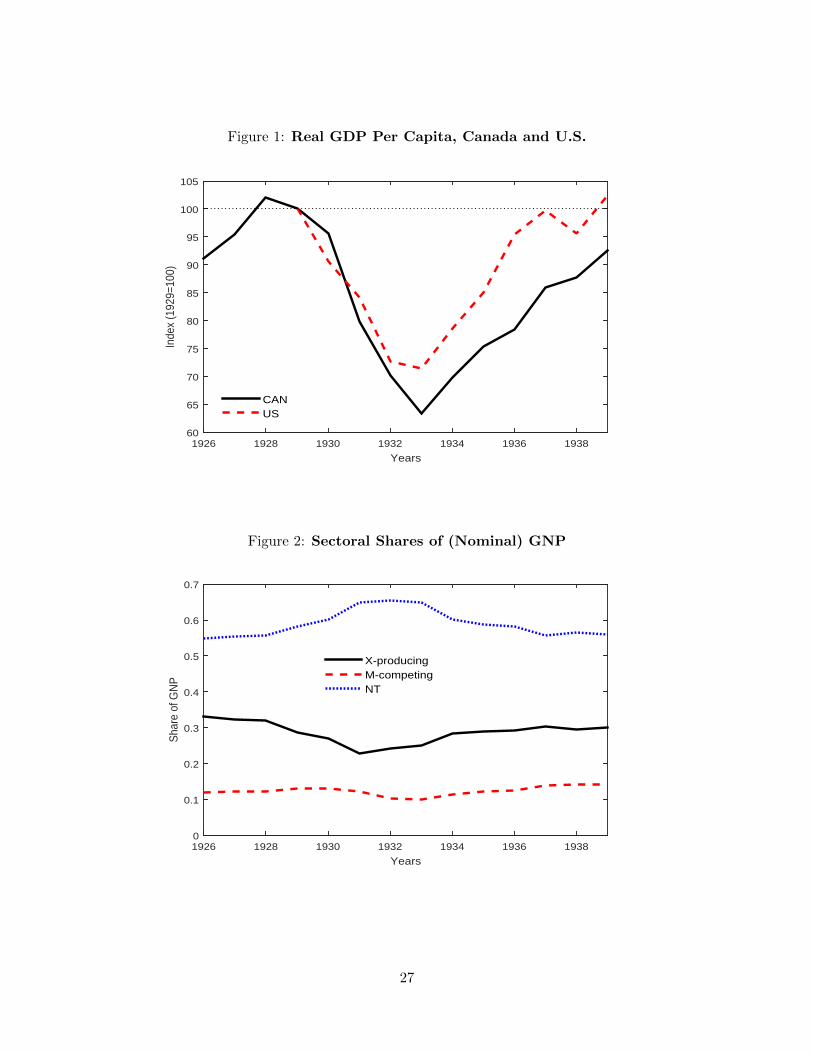
Figure 1: Real GDP Per Capita, Canada and U.S.

Years1926 1928 1930 1932 1934 1936 1938

Inde

x (1

929=

100)

60

65

70

75

80

85

90

95

100

105

CANUS

Figure 2: Sectoral Shares of (Nominal) GNP

Years1926 1928 1930 1932 1934 1936 1938

Sha

re o

f GN

P

0

0.1

0.2

0.3

0.4

0.5

0.6

0.7

X-producingM-competingNT

27

Figure 3: Trade Shares

Years1926 1928 1930 1932 1934 1936 1938

Sha

re o

f GD

P

0.2

0.22

0.24

0.26

0.28

0.3

0.32

X shareM share

Figure 4: Canadian Aggregate Price Indices

Years1926 1928 1930 1932 1934 1936 1938

Inde

x (1

926=

100)

65

70

75

80

85

90

95

100

GNE deflatorCOLIWPI

28

Figure 5: Prices: Exports, Imports and Nontradables

Years1926 1928 1930 1932 1934 1936 1938

Inde

x (1

926=

100)

60

65

70

75

80

85

90

95

100

105

110

AggregateX-producingM-competingNT

Figure 6: Canada: Traded vs Nontraded Prices

Years1926 1928 1930 1932 1934 1936 1938

Inde

x (1

926=

100)

60

65

70

75

80

85

90

95

100

105

TradedNon-tradedNon-traded ex-rent

29

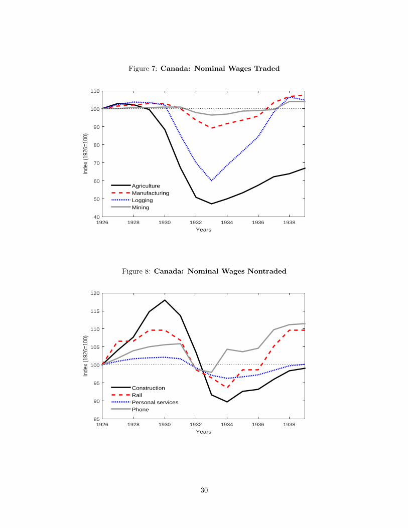
Figure 7: Canada: Nominal Wages Traded

Years1926 1928 1930 1932 1934 1936 1938

Inde

x (1

926=

100)

40

50

60

70

80

90

100

110

AgricultureManufacturingLoggingMining

Figure 8: Canada: Nominal Wages Nontraded

Years1926 1928 1930 1932 1934 1936 1938

Inde

x (1

926=

100)

85

90

95

100

105

110

115

120

ConstructionRailPersonal servicesPhone

30

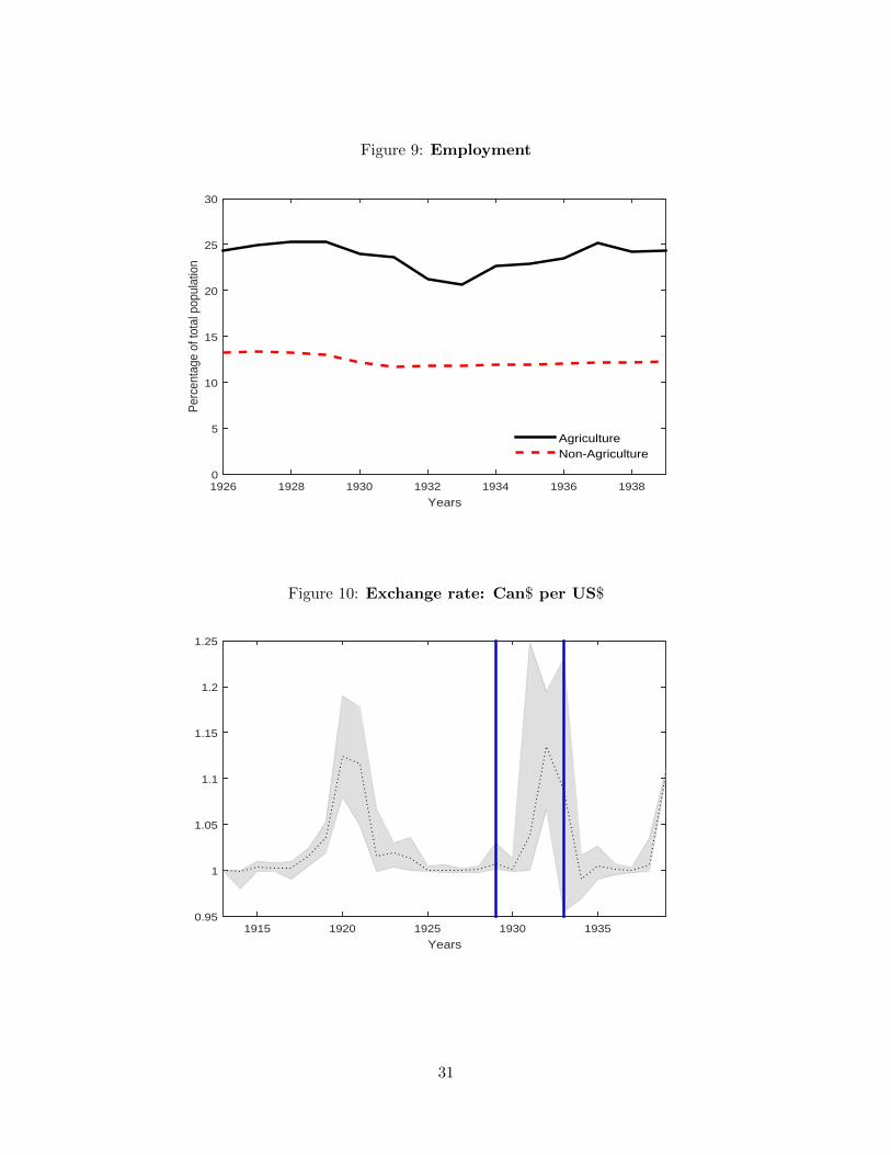
Figure 9: Employment

Years1926 1928 1930 1932 1934 1936 1938

Per

cent

age

of to

tal p

opul

atio

n

0

5

10

15

20

25

30

AgricultureNon-Agriculture

Figure 10: Exchange rate: Can$ per US$

Years1915 1920 1925 1930 1935

0.95

1

1.05

1.1

1.15

1.2

1.25

31

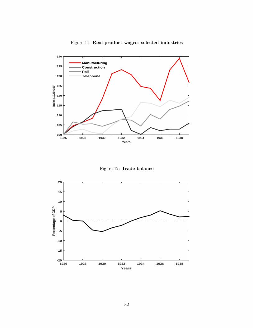
Figure 11: Real product wages: selected industries

Years1926 1928 1930 1932 1934 1936 1938

Inde

x (1

926=

100)

100

105

110

115

120

125

130

135

140

ManufacturingConstructionRailTelephone

Figure 12: Trade balance

Years1926 1928 1930 1932 1934 1936 1938

Perc

enta

ge o

f GD

P

-20

-15

-10

-5

0

5

10

15

20

32

Figure 13: Real output: frictionless model

Years1926 1928 1930 1932 1934 1936 1938

Inde

x (1

926=

100)

65

70

75

80

85

90

95

100

105

110

115

DataModel

Figure 14: Real output: nominal wage frictions

Years1926 1928 1930 1932 1934 1936 1938

Inde

x (1

926=

100)

65

70

75

80

85

90

95

100

105

110

115

DataModel

33

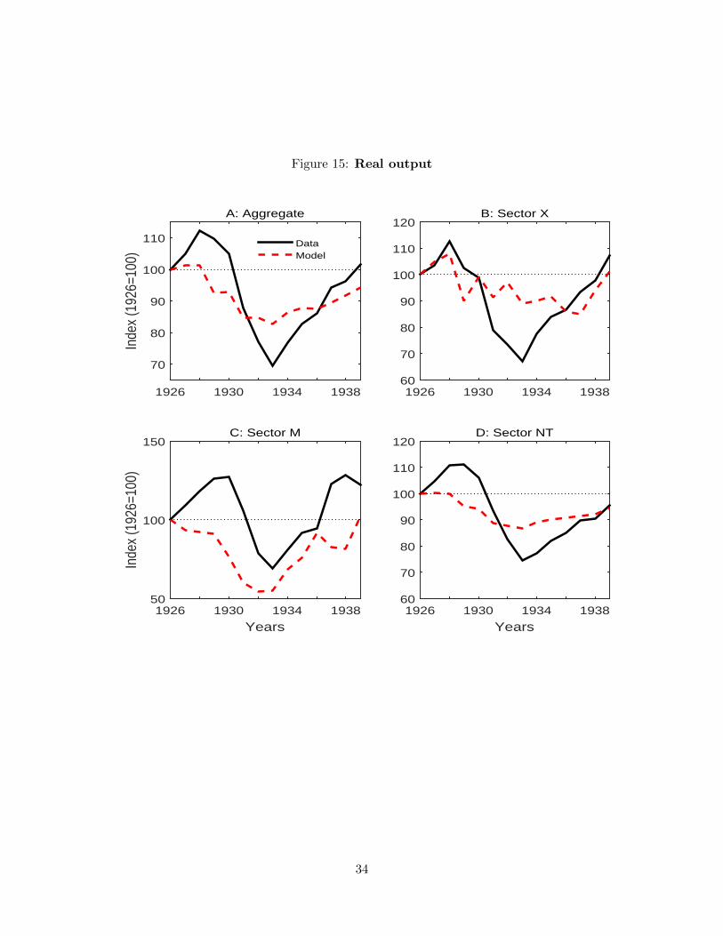
Figure 15: Real output

1926 1930 1934 1938

Inde

x (1

926=

100)

70

80

90

100

110

A: Aggregate

DataModel

1926 1930 1934 193860

70

80

90

100

110

120B: Sector X

Years1926 1930 1934 1938

Inde

x (1

926=

100)

50

100

150C: Sector M

Years1926 1930 1934 1938

60

70

80

90

100

110

120D: Sector NT

34

Figure 16: Prices

1926 1930 1934 1938

Inde

x (1

926=

100)

80

85

90

95

100A: Aggregate

DataModel

1926 1930 1934 193860

70

80

90

100B: Sector X

Years1926 1930 1934 1938

Inde

x (1

926=

100)

60

70

80

90

100C: Sector M

Years1926 1930 1934 1938

80

85

90

95

100

105

110D: Sector NT

35

Figure 17: Labor

1926 1930 1934 1938

Inde

x (1

926=

100)

70

80

90

100

110A: Aggregate

1926 1930 1934 193870

80

90

100

110B: Sector X

DataModel

Years1926 1930 1934 1938

Inde

x (1

926=

100)

40

60

80

100

120C: Sector M

Years1926 1930 1934 1938

70

80

90

100

110D: Sector NT

36

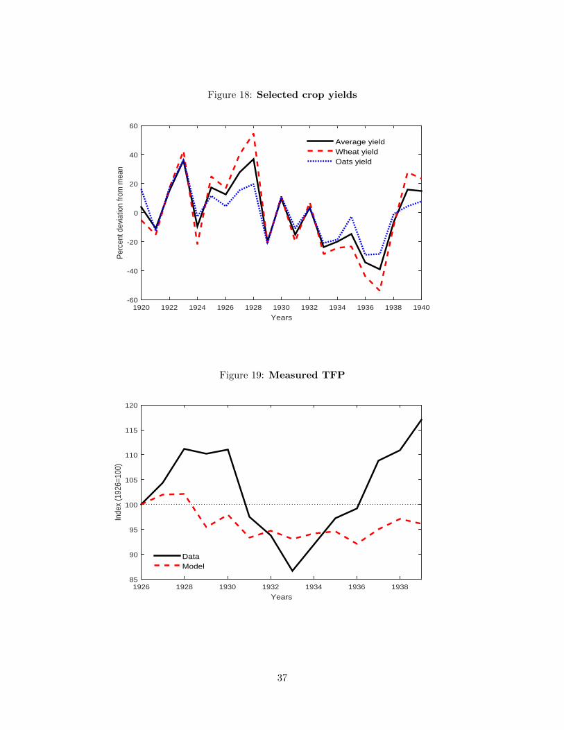
Figure 18: Selected crop yields

Years1920 1922 1924 1926 1928 1930 1932 1934 1936 1938 1940

Per

cent

dev

iatio

n fro

m m

ean

-60

-40

-20

0

20

40

60

Average yieldWheat yieldOats yield

Figure 19: Measured TFP

Years1926 1928 1930 1932 1934 1936 1938

Inde

x (1

926=

100)

85

90

95

100

105

110

115

120

DataModel

37

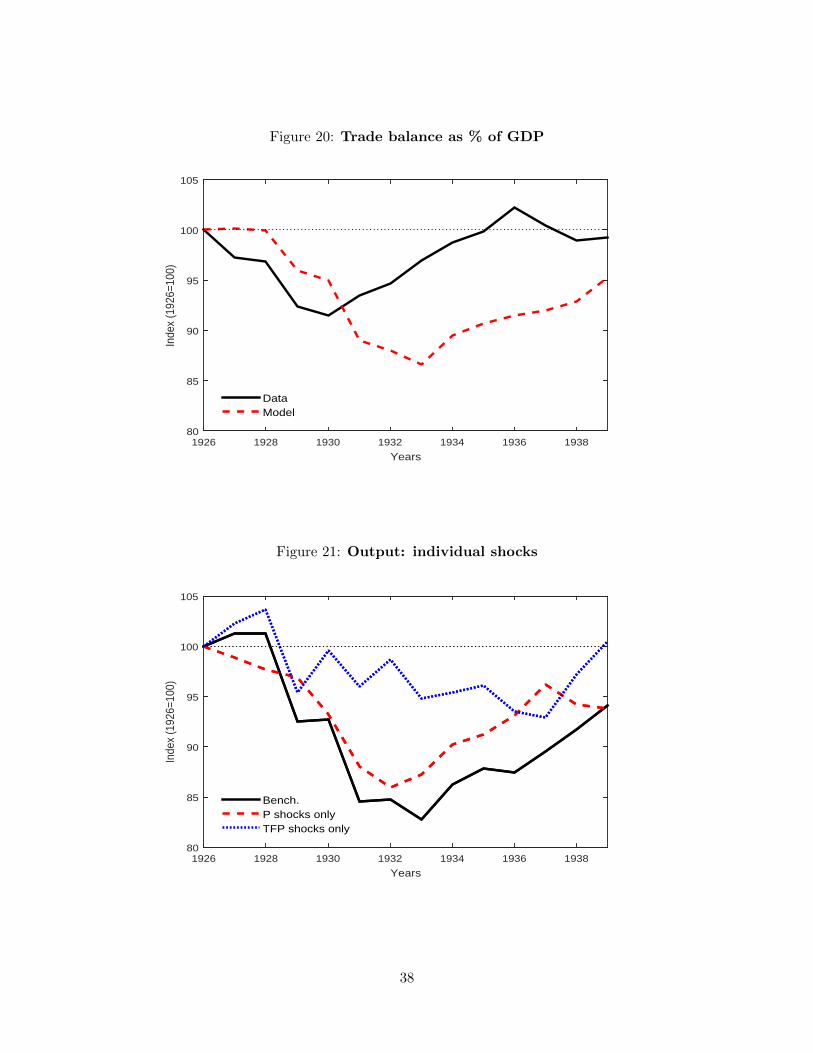
Figure 20: Trade balance as % of GDP

Years1926 1928 1930 1932 1934 1936 1938

Inde

x (1

926=

100)

80

85

90

95

100

105

DataModel

Figure 21: Output: individual shocks

Years1926 1928 1930 1932 1934 1936 1938

Inde

x (1

926=

100)

80

85

90

95

100

105

Bench.P shocks onlyTFP shocks only

38

Figure 22: Output: only one sticky-wage sector

Years1926 1928 1930 1932 1934 1936 1938

Inde

x (1

926=

100)

80

85

90

95

100

105

BenchmarkSticky NTSticky M

Figure 23: Output: adding monetary shocks

Years1926 1928 1930 1932 1934 1936 1938

Inde

x (1

926=

100)

82

84

86

88

90

92

94

96

98

100

102

Bench.M shocks

39

Figure 24: Sensitivity analysis

1926 1930 1934 1938

Inde

x (1

926=

100)

80

85

90

95

100

105

110A: Consumption elasticity

Bench.Low <High <

1926 1930 1934 193880

85

90

95

100

105

110B: Money elasticity

Bench.Low <

m

High <m

Years1926 1930 1934 1938

Inde

x (1

926=

100)

80

85

90

95

100

105

110C: Consumption substitutability

Bench.Low ;

c

High ;c

Years1926 1930 1934 1938

80

85

90

95

100

105

110D: Labor elasticity

Bench.Low <

l

High <l

40

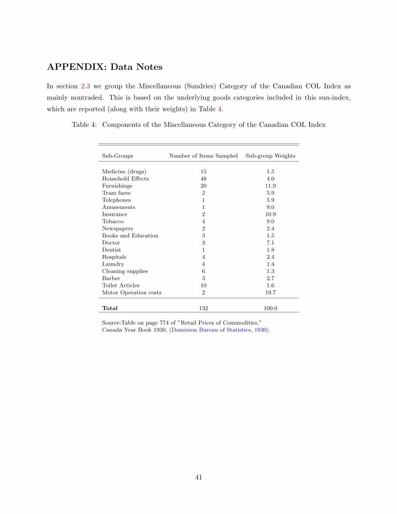
APPENDIX: Data Notes

In section 2.3 we group the Miscellaneous (Sundries) Category of the Canadian COL Index as

mainly nontraded. This is based on the underlying goods categories included in this sun-index,

which are reported (along with their weights) in Table 4.

Table 4: Components of the Miscellaneous Category of the Canadian COL Index

Sub-Groups Number of Items Sampled Sub-group Weights

Medicine (drugs) 15 1.5Household Effects 48 4.0Furnishings 20 11.9Tram fares 2 5.9Telephones 1 5.9Amusements 1 9.0Insurance 2 10.9Tobacco 4 9.0Newspapers 2 2.4Books and Education 3 1.5Doctor 3 7.1Dentist 1 1.8Hospitals 4 2.4Laundry 4 1.4Cleaning supplies 6 1.3Barber 3 2.7Toilet Articles 10 1.6Motor Operation costs 2 19.7

Total 132 100.0

Source:Table on page 774 of ”Retail Prices of Commodities,”Canada Year Book 1930, (Dominion Bureau of Statistics, 1930).

41