TEL-AVIV UNIVERSITY The Iby and Aladar Fleischman Faculty of Engineering TRADE-OFF BETWEEN RECOGNITION AND RECONSTRUCTION: APPLICATION OF NEURAL NETWORKS TO ROBOTIC VISION Thesis submitted for the degree ”Doctor of Philosophy” by INNA STAINVAS Submitted to the Senate of Tel-Aviv University 1999

Trade-off between recognition an reconstruction: Application of Robotics Vision to Face Recognition
Jan 27, 2015
Autonomous and ecient action of robots requires a robust robot vision system that can
cope with variable light and view conditions. These include partial occlusion, blur, and
mainly a large scale di erence of object size due to variable distance to the objects. This
change in scale leads to reduced resolution for objects seen from a distance. One of the
most important tasks for the robot's visual system is object recognition. This task is also
a ected by orientation and background changes. These real-world conditions require a
development of speci c object recognition methods.
This work is devoted to robotic object recognition. We develop recognition methods
based on training that includes incorporation of prior knowledge about the problem.
The prior knowledge is incorporated via learning constraints during training (parameter
estimation). A signi cant part of the work is devoted to the study of reconstruction
constraints. In general, there is a tradeo between the prior-knowledge constraints and
the constraints emerging from the classi cation or regression task at hand. In order to
avoid the additional estimation of the optimal tradeo between these two constraints, we
consider this tradeo as a hyper parameter (under Bayesian framework) and integrate
over a certain (discrete) distribution. We also study various constraints resulting from
information theory considerations.
Experimental results on two face data-sets are presented. Signi cant improvement in
face recognition is achieved for various image degradations such as, various forms of image
blur, partial occlusion, and noise. Additional improvement in recognition performance is
achieved when preprocessing the degraded images via state of the art image restoration
techniques.
Welcome message from author
This document is posted to help you gain knowledge. Please leave a comment to let me know what you think about it! Share it to your friends and learn new things together.
Transcript

TEL-AVIV UNIVERSITYThe Iby and Aladar Fleischman
Faculty of Engineering
TRADE-OFF BETWEEN RECOGNITION AND
RECONSTRUCTION:
APPLICATION OF NEURAL NETWORKS
TO ROBOTIC VISION
Thesis submitted for the degree ”Doctor of Philosophy”
by
INNA STAINVAS
Submitted to the Senate of Tel-Aviv University1999

TEL-AVIV UNIVERSITY
This work was carried out under the supervision of
Doctor Nathan Intrator
and
Doctor Amiram Moshaiov


This work is dedicated to my family


Acknowledgment
I would like to thank my husband, daughter and parents for their tolerance and moral
support during the completion of this thesis.
I am greatly indebted to my first advisor Dr. Amiram Moshaiov, who gave me a
chance to start as a Ph.D. Student at the Engineering Faculty of Tel-Aviv University,
when I was only two months in Israel. I am very grateful to him for proposing to work in
Neural Networks and Computer Vision and for allowing me freedom in my research.
I have been pleasantly surprised by the flexibility of the educational system of the Tel-
Aviv University in allowing me to listen and participate in courses at different faculties,
such as the Engineering Faculty, Computer Science and Foreign Languages.
While taking courses in Neural Networks, I met Dr. Nathan Intrator, who became my
main supervisor and collaborator for more than five years. He opened me to a new world
of Neural Networks and I have learned much from him, not only on the technical aspects
but also on scientific research methodologies. Without him, this thesis would have never
appear. I am grateful to him for his tolerance, endless support and guidance.
It is impossible to thank all the people who helped me, but I would like to mention the
system administrator of the Engineering faculty, Udi Mottelo, the Department secretary
Ariella Regev, the secretary of the Emigration Support department Ahuva, my friends,
and the people of the Neural Computation Group of Computer Science faculty, Yair
Shimshoni, Nurit Vatnick and Natalie Japkowich.
This work was supported by grants from the Rich Foundation, the Don and Sara
Marejn Scholarship Fund and by a grant from the Ministry of Science to Dr. Nathan
Intrator.
Inna Stainvas
March 8, 1999
Abstract
Autonomous and efficient action of robots requires a robust robot vision system that can
cope with variable light and view conditions. These include partial occlusion, blur, and
mainly a large scale difference of object size due to variable distance to the objects. This
change in scale leads to reduced resolution for objects seen from a distance. One of the
most important tasks for the robot’s visual system is object recognition. This task is also
affected by orientation and background changes. These real-world conditions require a
development of specific object recognition methods.
This work is devoted to robotic object recognition. We develop recognition methods
based on training that includes incorporation of prior knowledge about the problem.
The prior knowledge is incorporated via learning constraints during training (parameter
estimation). A significant part of the work is devoted to the study of reconstruction
constraints. In general, there is a tradeoff between the prior-knowledge constraints and
the constraints emerging from the classification or regression task at hand. In order to
avoid the additional estimation of the optimal tradeoff between these two constraints, we
consider this tradeoff as a hyper parameter (under Bayesian framework) and integrate
over a certain (discrete) distribution. We also study various constraints resulting from
information theory considerations.
Experimental results on two face data-sets are presented. Significant improvement in
face recognition is achieved for various image degradations such as, various forms of image
blur, partial occlusion, and noise. Additional improvement in recognition performance is
achieved when preprocessing the degraded images via state of the art image restoration
techniques.
Contents
1 Introduction 1
1.1 General motivation . . . . . . . . . . . . . . . . . . . . . . . . . . . . . . . 1
1.1.1 Robotic vision . . . . . . . . . . . . . . . . . . . . . . . . . . . . . . 1
1.1.2 Internal data representation . . . . . . . . . . . . . . . . . . . . . . 2
1.1.3 Data compression . . . . . . . . . . . . . . . . . . . . . . . . . . . . 3
1.1.4 Face recognition . . . . . . . . . . . . . . . . . . . . . . . . . . . . . 4
1.2 Overview of the thesis . . . . . . . . . . . . . . . . . . . . . . . . . . . . . 5
2 Statistical formulation of the problem 8
2.1 Bias-Variance error decomposition for a single predictor . . . . . . . . . . . 9
2.2 Variance control without imposing a learning bias . . . . . . . . . . . . . . 10
2.3 Variance control by imposing a learning bias . . . . . . . . . . . . . . . . . 12
2.3.1 Smoothness constraints . . . . . . . . . . . . . . . . . . . . . . . . . 12
2.3.2 Invariance bias constraints . . . . . . . . . . . . . . . . . . . . . . . 13
2.3.3 Specific bias constraints . . . . . . . . . . . . . . . . . . . . . . . . 14
2.4 Reconstruction bias constraints . . . . . . . . . . . . . . . . . . . . . . . . 16
2.5 Minimum Description Length (MDL) Principle . . . . . . . . . . . . . . . . 17
2.5.1 Minimum description length . . . . . . . . . . . . . . . . . . . . . . 19
2.6 Bayesian framework . . . . . . . . . . . . . . . . . . . . . . . . . . . . . . . 20
2.7 MDL in the feed-forward NN . . . . . . . . . . . . . . . . . . . . . . . . . 22
2.7.1 MDL and EPP bias constraints . . . . . . . . . . . . . . . . . . . . 24
2.8 Appendix to Chapter 2: Regularization problem . . . . . . . . . . . . . . . 28
3 Imposing bias via reconstruction constraints 30
3.1 Introduction . . . . . . . . . . . . . . . . . . . . . . . . . . . . . . . . . . . 30
3.1.1 Principal Component Analysis (PCA) . . . . . . . . . . . . . . . . . 30
3.1.2 Autoencoder network and MDL . . . . . . . . . . . . . . . . . . . . 31
3.1.3 Reconstruction and generative models . . . . . . . . . . . . . . . . 34
i

3.1.4 Classification via reconstruction . . . . . . . . . . . . . . . . . . . . 35
3.1.5 Other applications of reconstruction . . . . . . . . . . . . . . . . . . 38
3.2 Imposing reconstruction constraints . . . . . . . . . . . . . . . . . . . . . . 38
3.2.1 Reconstruction as a bias imposing mechanism . . . . . . . . . . . . 38
3.2.2 Hybrid classification/reconstruction network . . . . . . . . . . . . . 40
3.2.3 Hybrid network and MDL . . . . . . . . . . . . . . . . . . . . . . . 40
3.2.4 Hybrid network as a generative probabilistic model . . . . . . . . . 43
3.2.5 Hybrid Neural Network architecture . . . . . . . . . . . . . . . . . . 44
3.2.6 Network learning rule . . . . . . . . . . . . . . . . . . . . . . . . . . 46
3.2.7 Hybrid learning rule. . . . . . . . . . . . . . . . . . . . . . . . . . . 48
4 Imposing bias via unsupervised learning constraints 50
4.1 Introduction . . . . . . . . . . . . . . . . . . . . . . . . . . . . . . . . . . . 50
4.2 Information principles for sensory processing . . . . . . . . . . . . . . . . . 51
4.3 Mathematical background . . . . . . . . . . . . . . . . . . . . . . . . . . . 52
4.3.1 Entropy maximization (ME) . . . . . . . . . . . . . . . . . . . . . . 53
4.3.2 Minimization of the output mutual information (MMI) . . . . . . . 55
4.3.3 Relation to Exploratory Projection Pursuit. . . . . . . . . . . . . . 57
4.3.4 BCM . . . . . . . . . . . . . . . . . . . . . . . . . . . . . . . . . . . 59
4.3.5 Sum of entropies of the hidden units . . . . . . . . . . . . . . . . . 59
4.3.6 Nonlinear PCA . . . . . . . . . . . . . . . . . . . . . . . . . . . . . 60
4.3.7 Reconstruction issue . . . . . . . . . . . . . . . . . . . . . . . . . . 60
4.4 Imposing unsupervised constraints . . . . . . . . . . . . . . . . . . . . . . . 61
4.5 Imposing unsupervised and reconstruction constraints . . . . . . . . . . . . 62
5 Real world recognition 69
5.1 Introduction . . . . . . . . . . . . . . . . . . . . . . . . . . . . . . . . . . . 69
5.1.1 Face recognition . . . . . . . . . . . . . . . . . . . . . . . . . . . . . 69
5.2 Methodology . . . . . . . . . . . . . . . . . . . . . . . . . . . . . . . . . . 74
5.2.1 Different architecture constraints . . . . . . . . . . . . . . . . . . . 75
5.2.2 Regularization . . . . . . . . . . . . . . . . . . . . . . . . . . . . . . 76
5.2.3 Neural Network Ensembles . . . . . . . . . . . . . . . . . . . . . . . 80
5.2.4 Face data-sets . . . . . . . . . . . . . . . . . . . . . . . . . . . . . . 81
5.2.5 Face normalization . . . . . . . . . . . . . . . . . . . . . . . . . . . 81
5.2.6 Learning parameters . . . . . . . . . . . . . . . . . . . . . . . . . . 82
5.3 Type of image degradations . . . . . . . . . . . . . . . . . . . . . . . . . . 83
5.4 Experimental results . . . . . . . . . . . . . . . . . . . . . . . . . . . . . . 84
ii
5.4.1 Different architecture constraints and regularization ensembles . . . 86
5.5 Saliency detection . . . . . . . . . . . . . . . . . . . . . . . . . . . . . . . . 89
5.5.1 Saliency map . . . . . . . . . . . . . . . . . . . . . . . . . . . . . . 89
5.6 Conclusions . . . . . . . . . . . . . . . . . . . . . . . . . . . . . . . . . . . 94
5.7 Appendix to Chapter 5: Hidden representation exploration . . . . . . . . . 95
6 Blurred image recognition 100
6.1 Methodology . . . . . . . . . . . . . . . . . . . . . . . . . . . . . . . . . . 100
6.1.1 Experimental design . . . . . . . . . . . . . . . . . . . . . . . . . . 101
6.2 Image degradation . . . . . . . . . . . . . . . . . . . . . . . . . . . . . . . 102
6.2.1 Main filters . . . . . . . . . . . . . . . . . . . . . . . . . . . . . . . 103
6.2.2 Other types of degradation . . . . . . . . . . . . . . . . . . . . . . . 106
6.3 Image restoration . . . . . . . . . . . . . . . . . . . . . . . . . . . . . . . . 107
6.3.1 MSE minimization and regularization . . . . . . . . . . . . . . . . . 107
6.3.2 Image restoration in the frequency domain . . . . . . . . . . . . . . 109
6.3.3 Denoising . . . . . . . . . . . . . . . . . . . . . . . . . . . . . . . . 111
6.4 Results . . . . . . . . . . . . . . . . . . . . . . . . . . . . . . . . . . . . . . 111
6.4.1 Image filtering . . . . . . . . . . . . . . . . . . . . . . . . . . . . . . 112
6.4.2 Classification of noisy data . . . . . . . . . . . . . . . . . . . . . . . 114
6.4.3 Gaussian blur . . . . . . . . . . . . . . . . . . . . . . . . . . . . . . 115
6.4.4 Motion blur . . . . . . . . . . . . . . . . . . . . . . . . . . . . . . . 117
6.4.5 Blind deconvolution . . . . . . . . . . . . . . . . . . . . . . . . . . . 118
6.4.6 All training schemes . . . . . . . . . . . . . . . . . . . . . . . . . . 120
6.5 Conclusions . . . . . . . . . . . . . . . . . . . . . . . . . . . . . . . . . . . 121
7 Summary and future work 124
7.1 Summary . . . . . . . . . . . . . . . . . . . . . . . . . . . . . . . . . . . . 124
7.2 Directions for future work . . . . . . . . . . . . . . . . . . . . . . . . . . . 126
iii

List of Figures
2.1 Supervised feed-forward network . . . . . . . . . . . . . . . . . . . . . . . . 23
2.2 Hybrid network with EPP constraints . . . . . . . . . . . . . . . . . . . . . 25
3.1 Autoencoder network architecture . . . . . . . . . . . . . . . . . . . . . . . 32
3.2 Eigenspaces extracted by PCA . . . . . . . . . . . . . . . . . . . . . . . . . 36
3.3 Combined recognition/reconstruction network . . . . . . . . . . . . . . . . 40
3.4 Hybrid network with reconstruction and EPP constraints . . . . . . . . . . 41
3.5 Detailed architecture of the recognition/reconstruction network . . . . . . 45
4.1 Feed-forward network for independent component extraction . . . . . . . . 53
4.2 Pdf’s graphs for a family of the exponential density functions . . . . . . . . 65
4.3 Exploratory projection pursuit network . . . . . . . . . . . . . . . . . . . . 66
5.1 Misclassification rate time evolution . . . . . . . . . . . . . . . . . . . . . . 77
5.2 MSE (mean-squared) recognition error time evolution . . . . . . . . . . . . 78
5.3 Classification based regularization . . . . . . . . . . . . . . . . . . . . . . . 79
5.4 “Caricature” faces in three resolutions . . . . . . . . . . . . . . . . . . . . 81
5.5 Image degradation and reconstruction (TAU data-set) . . . . . . . . . . . . 84
5.6 Summary of different networks and different image degradations . . . . . . 90
5.7 Saliency map construction . . . . . . . . . . . . . . . . . . . . . . . . . . . 91
5.8 Hidden unit activities vs. classes - for an unconstrained network . . . . . . 96
5.9 Hidden unit activities vs. classes - for a reconstruction network . . . . . . . 97
5.10 Pdf’s of the hidden unit activities . . . . . . . . . . . . . . . . . . . . . . 98
5.11 Hidden weight representation . . . . . . . . . . . . . . . . . . . . . . . . . 99
6.1 Experimental design schemes . . . . . . . . . . . . . . . . . . . . . . . . . . 102
6.2 Training scheme C . . . . . . . . . . . . . . . . . . . . . . . . . . . . . . . 103
6.3 Degraded images . . . . . . . . . . . . . . . . . . . . . . . . . . . . . . . . 104
6.4 Noisy Images . . . . . . . . . . . . . . . . . . . . . . . . . . . . . . . . . . 115
6.5 Gaussian blur and restoration . . . . . . . . . . . . . . . . . . . . . . . . . 116
iv

6.6 Motion blur and deblur . . . . . . . . . . . . . . . . . . . . . . . . . . . . . 118
6.7 Blind deconvolution . . . . . . . . . . . . . . . . . . . . . . . . . . . . . . . 119
6.8 Recognition of blurred images via schemes A–C . . . . . . . . . . . . . . . 120
6.9 Reconstruction of Gaussian blurred images . . . . . . . . . . . . . . . . . . 123
v

List of Tables
4.1 Unsupervised constraints . . . . . . . . . . . . . . . . . . . . . . . . . . . . 62
5.1 Classification results for Pentland data-set . . . . . . . . . . . . . . . . . . 85
5.2 Different ensemble types (Pentland data-set) . . . . . . . . . . . . . . . . . 87
5.3 Different ensemble types (TAU data-set) . . . . . . . . . . . . . . . . . . . 88
5.4 Recognition using saliency map (Pentland data-set) . . . . . . . . . . . . . 92
5.5 Recognition using saliency map (TAU data-set) . . . . . . . . . . . . . . . 93
6.1 Classification results for filtered data . . . . . . . . . . . . . . . . . . . . . 112
6.2 Noise and restoration . . . . . . . . . . . . . . . . . . . . . . . . . . . . . . 114
6.3 Gaussian blur and restoration . . . . . . . . . . . . . . . . . . . . . . . . . 115
6.4 Motion blur and restoration . . . . . . . . . . . . . . . . . . . . . . . . . . 117
6.5 Blind deconvolution . . . . . . . . . . . . . . . . . . . . . . . . . . . . . . . 119
6.6 Blurred image recognition via joined ensembles . . . . . . . . . . . . . . . . 121
7.1 Classification error for reconstructed images . . . . . . . . . . . . . . . . . 127
vi

Chapter 1
Introduction
1.1 General motivation
1.1.1 Robotic vision
Nowadays, robots that can move and operate autonomously in a real-world are in high
demand. One of the main perception tasks that has to be addressed in this context is a
recognition task. The recognition task in a real-world environment is challenging as it has
to address data variability, such as orientation, changing background, partial occlusion
and blur, etc.
For illustration let us consider a vision-guided robot helicopter which has to navigate
autonomously using only on-board sensors and computing power (Chopper, 1997). One
of the basic difficulties in recognition of images taken by helicopter cameras during an op-
eration is the significant difference between these images and the images, which the robot
is acquainted with in ideal flight conditions. Usually, the images taken during operation
contain a large amount of degradation caused by diverse factors, such as illumination
changing, bad weather conditions, relative motion between the cameras and the object
of interest in the scene, shadows and, low resolution capacity of the cameras, etc. Some
of these factors cause images to look blurred and foggy, others lead to noise and partial
occlusion. All these factors are crucial for recognition performance and require special
care.
Among the possible approaches to improve recognition performance of degraded im-
ages is an endeavor to recover images using state of the art restoration techniques as
preprocessing before a recognition stage. This preprocessing requires estimation of the
degradation process, e.g. the type and parameters of the blur operation. Another ap-
proach is to directly address the variability in the recognition system. It is well known
that for a restoration process to be successful a degradation process has to be accurately
1

Chapter 1: Introduction 2
modeled. However, in many cases, an exact modeling is impractical, and the restored im-
ages remain partially degraded and contain artifacts. Furthermore, restoration methods
are often computationally expensive and require a-priori knowledge or human interaction.
It follows that efforts have to be concentrated on development of recognition methods that
are more robust to image degradations.
1.1.2 Internal data representation
An important aspect of robust recognition methods is construction of an internal data
representation (feature extraction), that captures the significant structure of the data.
According to D. Marr (1982) finding an internal representation is an inherent component
of the vision process.
Feature based representation Many recognition methods include grouping or per-
ceptual organization as a first stage of the visual processing. In this stage, objects are
represented as models, containing the essential features and logic tight rules needed for
recognition. Some methods extract “anchor points” (Ullman, 1989; Brunelli and Poggio,
1992), others consider edge segments as interesting feature elements (Bhanu and Ming,
1987; Liu and Srinath, 1984). A relatively new approach is a deformable template match-
ing (Grenander, 1978; Brunelli and Poggio, 1993; Jain et al., 1996) and using generalized
splines for object classification (Lai, 1994). These methods attempt to extract salient
features locally in the low level stage of the visual processing, according to subjective
understanding of an investigator. Therefore, finding an internal representation based on
extraction of object features and relation between them may be limited.
Learning internal representations via Neural Networks A radical alternative
approach is to use all the available intensity information for finding internal representation.
Principal Component Analysis (PCA) (Fukunaga, 1990) is a non neural network example
of this approach, where internal representation space is spanned by the largest eigenvectors
of the data covariance matrix. These eigenvectors are macro-features extracted implicitly
from the images. When fed with intensity images, Neural Networks similar to PCA extract
internal representation in the space of hidden unit activities.
Processing an image as a whole is a high dimensional recognition task that leads to
the curse of dimensionality (Bellman, 1961) which means that there is not enough data
to robustly train a classifier in a high dimensional space. As an example, a network with
a single hidden unit and input images of 60× 60 pixels has 3600 weight parameters that
have to be estimated. Thus, the main issue is finding an intrinsic low dimensional

Chapter 1: Introduction 3
representation of the images. As was pointed out by Geman et al. (1992), a way to avoid
the curse of dimensionality in Neural Networks is to prewire the important generalizations
by purposefully introducing learning bias.
The work presented in this thesis is specifically devoted to this issue. We develop
image recognition techniques using hybrid feed-forward Neural Networks, obtained by
introducing a learning bias. In particular, we investigate the influence of the novel re-
construction learning constraints on the recognition performance of feed-forward Neural
Networks. In addition, we propose to use other learning constraints based on information
theory, and subsequently compare their efficiency with reconstruction learning constraints.
We demonstrate that hybrid Neural Networks are robust to real-world degradation in the
input visual data and show that their performance can be further enhanced when state
of the art (deblur) techniques are also incorporated.
1.1.3 Data compression
Often, a compression goal is defined as finding a compact data representation leading to
good data reconstruction. Principal Component Analysis (PCA), Discrete Fourier Trans-
form (DFT) and its generalization, Wavelet Transform and advanced best basis repre-
sentations (Coifman and Wickerhauser, 1992), are examples of compression techniques.
Compression may be also realized via an autoencoder network (Cottrell et al., 1987). The
autoencoder is a multi layer perceptron (MLP) type of the network with the output layer
coinciding with the input layer and a hidden layer of a small size.
Recently a novel type of an autoencoder network has been proposed by Zemel (1993).
The hidden layer is allowed to have a large number of hidden units but it has different con-
straints on the developed hidden representation. The network is simultaneously trained
to accurately reconstruct the input and to find a succinct representation in the hidden
layer, assuming sparse or population code formation in the autoencoder hidden layer.
When the main task is recognition, the compressed data representation has been used
instead of the original (high-dimensional) data (Kirby and Sirovich, 1990; Turk and Pent-
land, 1991; Murase and Nayar, 1993; Bartlett et al., 1998). Recognition from this rep-
resentation is faster and may have better generalization performance. However, it is
clear, that such compression is task-independent and may be inappropriate for a specific
recognition task (Huber, 1985; Turk and Pentland, 1993).
We seek a compact data description that is task-dependent, and is good for recognition.
Thus, the quality of the compression scheme is judged by its generalization property.
Often, a separate low-dimensional representation is created for every specific task at hand.
Another strategy could be to discover a hidden representation that is suitable for several

Chapter 1: Introduction 4
potential visual tasks (Intrator and Edelman, 1996). We show that a good task-dependent
compression is obtained when the data representation is constructed not only to minimize
the mean-squared recognition error, but also to maintain data fidelity and/or to extract
good statistical properties. These good properties may be the independence of hidden
neurons, maximum information transfer in the hidden layer or a multi-modal distribution
of the hidden unit activities. Therefore, in this case compression is task-dependent and is
assisted by the a-priori knowledge.
In summary, we investigate lossy compression techniques based on the two visual tasks
- image recognition and reconstruction. Our goal is to find a hidden representation that
optimizes the recognition using hints of the reconstruction task.
1.1.4 Face recognition
The performance of the proposed recognition schemes is examined on two facial data
sets. Face recognition has gained much attention in recent years due to the variety of
commercial applications, such as video conferencing, security, human communication and
robotics. Face recognition has recently attracted special attention of different human
robotic groups, that intensively work on the creation of personal adaptive robots to assist
the frail and elderly blind people, and creation of working mobile robots for delivery
assistance (Hirukawa, 1997; Connolly, 1997).
This recognition task is a very difficult one (Chellapa et al., 1995), since it is a high di-
mensional classification problem leading to “curse of dimensionality”. This is complicated
by the large variability of the facial data sets due to:
• viewpoint dependence
• nonrigidity of the faces
• variable lighting conditions
• motion
The task of face recognition is a particular case of the learning when the variability of
the data describing the same class is comparable with the similarity between different
classes. Other important possible recognition tasks from the same category may be the
recognition of different kinds of tanks, ships, planes and cars, etc.

Chapter 1: Introduction 5
1.2 Overview of the thesis
The thesis focuses on developing Neural Network techniques that improve the recognition
performance. A key aspect of this work is finding data representations that lead to better
generalization. We show that networks which are trained to recognize and reconstruct
images simultaneously extract features that improve recognition. Improved performance
is also achieved when networks are trained to find other statistical structures in the data.
The thesis is organized as follows:
Chapter 2: Formulates the recognition task in the framework of the “bias-variance”
dilemma. We show that for a good generalization ability the variance portion of the
generalization error has to be properly controlled. We discuss different methods to control
the variance portion of the generalization error and present two main approaches: reducing
the variance via ensemble averaging and introducing a learning bias. We review different
types of learning bias constraints, and finally, propose reconstruction constraints as a
novel type of bias constraints in the context of feed-forward networks.
Starting from Section 2.5, we discuss the relation between the “bias-variance” dilemma
in statistics, MDL principle and Bayesian framework. We show that the introduction of
a learning bias corresponds to a model-cost in the description length, which has to be
minimized along with an error-cost under the MDL principle. At the same time, under
the Bayesian framework, the model-cost corresponds to prior knowledge about the weights
and hidden representation distributions.
Chapter 3: Introduces a hybrid feed-forward network architecture, which uses the re-
construction constraints as a bias imposing mechanism for the recognition task. This net-
work, which can be interpreted under MDL and Bayesian frameworks, modifies the low
dimensional representation by minimizing concurrently the mean squared error (MSE)
of reconstruction and classification outputs. In other words, it attempts to improve the
quality of the hidden layer representation by imposing a feature selection useful for both
tasks, classification and reconstruction. A significance of each of the tasks is controlled
by a trade-off parameter λ, which is interpreted as a hyper-parameter in the Bayesian
framework. Finally, this chapter presents technical details about the network architecture
and its learning rule.
Chapter 4: Discusses various information theory principles as constraints for the clas-
sification task. We introduce a hybrid neural network with a hidden representation which

Chapter 1: Introduction 6
has some useful properties, such as the independence between hidden layer neurons or
maximum information transfer in the hidden layer, etc.
Chapter 5: Discusses the face recognition task. We review different Neural Networks
methods used for face recognition and apply the hybrid networks introduced in Chap-
ters 3–4. This chapter contains technical details related to face normalization and learn-
ing procedures. It is shown that the best regularized network is impractical for degraded
image recognition, and integration over different regularization parameters and different
initial weights is preferable. This integration is roughly approximated by averaging over
network ensembles. We consider three ensemble types: Unconstrained ensemble that cor-
responds to integration over initial weights and fixed trade-off parameter λ = 0, i.e. the
hidden representation is based on the recognition task alone; Reconstruction ensemble
that corresponds to integration over different values of the trade-off parameter λ for fixed
initial weights. Joined ensemble that corresponds to integration over both the trade-off
parameter λ and initial weights and is obtained by merging unconstrained and reconstruc-
tion ensembles.
Classification results on the degraded images, such as noisy, partially occluded and
blurred images are presented. We show that the joined ensemble is superior to the recon-
struction ensemble, which in turn is superior to the unconstrained ensemble. Finally we
conclude that reconstruction constraints improve generalization, especially under image
degradations. In addition we show that via saliency maps (Baluja, 1996) reconstruction
can deemphasize degraded regions of the input, thus leading to classification improvement
under “Salt and Pepper” noise.
Chapter 6: Addresses recognition of blurred and noisy images. In practice, images
appear blurred due to motion, weather conditions and camera defocusing. Several meth-
ods that address recognition of blurred images are proposed: (i) Expansion the training
set with Gaussian blurred images; (ii) Constraining reconstruction of blurred images to
the original images during training; (iii) Usage of state of the art restoration methods as
preprocessing to degraded images.
Three types of joined ensembles were considered and compared: Ensemble of networks
trained on the original training data only, and ensembles trained on the training set
expanded with Gaussian blurred images and with reconstruction constraints of two types,
where the first is a simple duplication of the input in the output and second as described
above in (ii).
It was shown that training with blurred images leads to a robust classification result

Chapter 1: Introduction 7
under different types of the blur operations and is more important than the restoration
methods.
Chapter 7: Summarizes our research and gives some perspective to its future develop-
ment, such as:
• Testing the hybrid architecture performance on the non face data sets of similar
object images, such as military, medical and astronomical
• Ensemble interpretation
• Using the recurrent network architecture
• Weighted network ensemble averaging based on the different error types between
input and output reconstruction layers
• Using invariance constraints (tangent prop like, see Chapter 2) regularization terms
for different types of blur operations for both recognition and reconstruction tasks
• Generalization of the proposed hybrid network on the other types of the generative
(reconstruction) models constrained by the classification task
Chapter 2
Statistical formulation of theproblem
Images as input to Neural Networks are a very high dimensional data with the size equal
to the number of pixels in the image. In this case, the number of the network weight
parameters is considerably larger than the size of the training set. This leads to the
curse of dimensionality (Bellman, 1961), which means that there is not enough data
to robustly train a classifier in a high dimensional space. Until recently, estimation in
such cases sounded unrealistic, but it is now accepted that such estimation is possible
if the actual dimensionality of the input data is much smaller. In other words, a true,
intrinsic dimensionality reduction is possible. A simple dimensionality reduction solely
via a bottleneck network architecture does not cope with the problem, since a network
continues to be an over-parameterized model (i.e. the number of free weight parameters
remains large).
It is well known that an estimation error is composed of two portions, bias and variance
(Geman et al., 1992). The over-parameterized models usually have a small bias (unless
they are incorrect), but have high variance, since the available data is always small com-
pared to the number of the free parameters and this leads to a high sensitivity to noise
in the training data. To robustify the estimator, the variance portion of the error has
to be controlled. One of the ways to control variance is via averaging single estimators
trained on the same task. The other method controls variance by introducing a learning
bias as constraints on the network architecture. Different types of smoothing constraints
are widely spread (Wahba, 1990; Murray and Edwards, 1993; Raviv and Intrator, 1996;
Munro, 1997). However, as has been pointed out by Geman et al. (Geman et al., 1992)
to solve the bias/variance dilemma innovative bias constraints have to be used. Introduc-
tion of these constraints into the network model leads naturally to a true dimensionality
reduction (Intrator, 1999).
8

Chapter 2: Statistical formulation of the problem 9
Below, we present the bias-variance dilemma and review methods to control the vari-
ance and bias portions of the prediction error. Then we propose to use image reconstruc-
tion as an innovative bias constraint for image classification. We proceed with discussion
on the relation between the “bias-variance” dilemma in statistics, MDL principle and
Bayesian networks.
2.1 Bias-Variance error decomposition for a single
predictor
The basic objective of the estimation problem is to find a function fD(x) = f(x;D) given a
finite training set D, composed of n input/output pairs, D = (xµ, yµ)nµ=1 x ∈ Rd,y ∈R1, drawn independently according to an unknown distribution P (x, y), which “best”
approximates the “target” function y (Geman et al., 1992).
Evaluation of the performance of the estimator is usually done via a mean squared
error by taking the expectation with respect to a marginal probability P (y|x):
E(x;D) ≡ E[(y − fD(x))2|x,D] = E[(y − E[y|x])2|x,D]︸ ︷︷ ︸V ar(y|x)
+E[(fD(x)− E[y|x])2|x,D]︸ ︷︷ ︸+
2E[(y − E[y|x])(fD(x)− E[y|x])|x,D]︸ ︷︷ ︸=0
(2.1.1)
It can be seen that the third term in the sum is equal to zero, since (fD(x) − E[y|x])
does not depend on the distribution P (y|x) and plays the role of a factor, while E[(y −E[y|x])|x,D] is equal to zero. The first term does not depend on the predictor f and
measures the variability of y given x (in the model with additive independent noise y =
f(x) + η(x) this term measures a noise variance in x). The contribution of the second
term can be reduced by optimizing f . This term measures the squared distance between
the estimator fD(x) and the mean of y given x (E[y|x]).
A good estimator has to generalize well to new sets drawn from the same distribution
P (y,x). A natural measure of the estimator effectiveness is an average error E(x) ≡ED[E(x;D)] = ED[E[(y − fD(x))2|x,D]] over all possible training sets D of fixed size:
E(x) = V ar(y|x)︸ ︷︷ ︸intrinsic error
+ (ED[fD(x)]− E[y|x])2
︸ ︷︷ ︸squared bias b2(f |x)
+ED[(fD(x)− ED[fD(x)])2]︸ ︷︷ ︸variance var(f |x)
(2.1.2)
The first term is an intrinsic error that can not be altered. If on average, fD(x) is
different from E[y|x], then fD(x) is biased. As we can see, an unbiased estimator may
still have a large mean squared error if the variance is large. Thus, either bias or variance
can contribute to poor performance (Geman et al., 1992). When training with a fixed
Chapter 2: Statistical formulation of the problem 10
training set D, reducing the bias with respect to this set may increase the variance of
the estimator and contribute to poor generalization performance. This is known as the
tradeoff between variance and bias.
2.2 Variance control without imposing a learning bias
The variance portion of a prediction error can sometimes be reduced without a bias in-
troduction by ensemble averaging. An ensemble (committee) is a combination of single
predictors trained on the same task. For example, in neural networks, an ensemble is a
combination of individual networks that are trained separately and then their predictions
are combined. This combination is done by majority or plurality rules (in classification)
(Hansen and Salamon, 1990) or by a weighted linear combination of predictors in regres-
sion (Meir, 1994; Naftaly et al., 1997). The plurality rule is defined as the decision agreed
by the majority of networks. The majority rule is defined as the decision agreed by
more than half of the networks, otherwise the ensemble rejects to classify and an error is
reported. The most general method to create ensemble has been presented by Wolpert
(Wolpert, 1992). The method is called stacked generalization and a non-linear network
learns how to combine the network outputs with the weights that vary over the feature
space.
It is well known that ensemble is useful if its individual predictors are independent
in their errors or disagree on some inputs. Thus, the main question is to find network
candidates that achieve this independence. One of the widely spread methods to create
neural network ensembles is based on the fact that neural networks are non-identifiable
models, i.e. the selection of the weights is an optimization problem with many local
minima. Thus, a network ensemble is created by varying the set of initial random weights
(Perrone, 1993). Another way is to use different types of predictors, like a mixture of
networks with a different topology and complexity or a mixture of networks with completely
different types of learning rules (Jacobs, 1997). Another way is to train the networks on
different training sets. Below, a bias-variance error decomposition for a weighed linear
combination of predictors is presented (Raviv, 1998; Tesauro et al., 1995).
Let us consider M predictors fi(x,Di), each trained on a training set Di. All training
sets have the same size and are drawn from the same joint distribution P (y,x). Consider
the ensemble based on the linear combination of predictors:
fens(x) =∑
i
aifi(x,Di),∑
i
ai = 1, ai ≥ 0, i = 1, 2, . . . ,M. (2.2.3)
Chapter 2: Statistical formulation of the problem 11
The normalization condition∑i ai = 1 is implied to make an ensemble unbiased, when
each individual estimator fi is unbiased. Let us consider the error (2.1.2) for this ensemble:
Eens(x) = V ar(y|x) + b2(fens|x) + var(fens|x), (2.2.4)
where the bias b(fens|x) is given as:
b(fens|x) = ED1,D2,...,DM [∑
i
aifi(x,Di)− E[y|x]] =
∑
i
aiEDi [fi(x,Di)− E[y|x]] =∑
i
aib(fi|x). (2.2.5)
Thus the bias of the ensemble is the same linear combination of the biases of the estima-
tors. Expanding the ensemble variance term we get:
var(fens|x) = ED1,D2,...,DM [∑i
aifi(x,Di)− ED1,D2,...,DM [∑
i
aifi(x,Di)]2] =
ED1,D2,...,DM [(∑
i
aifi(x,Di)−∑
i
aiEDi [fi(x,Di)])2] =
ED1,D2,...,DM [(∑
i
ai(fi(x,Di)− EDi [fi(x,Di)])2] =
ED1,D2,...,DM [∑
i
a2i (fi(x,Di)− EDi [fi(x,Di)])2 +
2∑
i>j
aiaj(fi(x,Di)− EDifi(x,Di))(fj(x,Dj)− EDjfj(x,Dj))] =
=∑
i
a2i var(fi|x) + 2
∑
i>j
aiajEDi,Dj [(fi − EDi [fi])(fj − EDj [fj])]
Finally, we get the next expression for the ensemble error:
Eens(x) = V ar(y|x) + (∑
i
aib(fi|x))2 +∑
i
a2i var(fi|x)
+2∑
i>j
aiajEDi,Dj [(fi − EDi [fi])(fj − EDj [fj])] (2.2.6)
If all estimators are unbiased, uncorrelated and have identical variances, simple averaging
with the same weights ai = 1/M leads to the following ensemble error (Raviv, 1998):
E(x) = V ar(y|x) + b2(f |x) +1
Mvar(f |x).
This decomposition shows that when biases are small and predictors are independent a
significant reduction of order 1/M in the variance may be attained.
If estimators are unbiased and uncorrelated it is easy to show that optimal weights
have to be inversely proportional to the variance of the individual predictors ai ∝ 1var(fi|x)
,
(Tresp and Taniguchi, 1995; Taniguchi and Tresp, 1997). Intuitively it means that a
predictor that is uncertain about its own prediction should obtain a smaller weight.

Chapter 2: Statistical formulation of the problem 12
2.3 Variance control by imposing a learning bias
A regression function (E[y|x]) is the best estimator. In order to find an unbiased estimator,
a family of possible estimators has to be abundant. In the MLP (multi-layer perceptron)
networks, this may be attained at the expense of network architecture growing. This
eliminates bias, but increases variance unless the training data is infinite. In practice, the
training data is finite and the main question is to make both a bias and variance “small”
using finite training sets (Geman et al., 1992). Geman et al. point out that in this
limitation the learning task is to generalize in a very nontrivial sense, since the training
data will never “cover” a space of possible inputs. This extrapolation is possible, if the
important generalizations are prewired in learning algorithms by purposefully introducing
a bias.
The most general and weakest a-priori constraints assume that mapping is smooth.
Other, stronger a-priori constraints may be expressed as an invariance of the mapping
to some group of transformation or an assumption about the class of possible mapping.
Another type of specific bias constraints appears when a supervised task is learned in
parallel with its other related tasks.
One way to categorize different types of constraints into two groups: variance and
bias constraints, has been proposed in (Intrator, 1999). Both types of constraints serve
to reduce the variance portion of the generalization error, however they have a different
effect on the bias portion of the error. Variance constraints always result in an increase of
the bias portion of the error. In contrast, bias constraints assist in learning and even may
reduce the bias portion of the error. When networks are learned to satisfy constraints only,
the bias constraints lead to a meaningful hidden representation, capturing the structure
of the input domain; while a hidden representation extracted via the variance constraints
is less interesting.
2.3.1 Smoothness constraints
The easiest way to smooth the mapping approximated by neural networks is by controlling
network structure parameters such as numbers of hidden units and hidden layers. The
larger is the number of network units, the larger is the number of weight fitting parameters.
The over-parameterized models are highly flexible and reduce bias. However, they are
sensitive to noise that leads to a large variance and a large generalization error. Another
way to control smoothness in neural networks, borrowed from the spline theory (Wahba,
1990), is to use weight decay. This involves adding a penalty term controlling a weight’s
norm, to the network cost function E =∑i ‖ yi − f(xi, ω) ‖2 (other forms of cost functions
Chapter 2: Statistical formulation of the problem 13
are presented in (Bishop, 1995a)):
Eλ = E + λ ‖ ω ‖2,
where xi and yi are the suitably scaled input and output samples (‖ z ‖ is the norm
in the space of the element z). Another tightly related approach is to constrain a range
of the weights to some middle values. The method is called weight elimination and the
regularization term has the form λ∑i ω
2i /(ω
2i + ω2
i0). A direct approach is to consider a
regularizer which penalizes curvature explicitly:
Eλ = E + λ ‖ P f ‖2,
where P is a differential operator. Another way to control the smoothness is to inject noise
during the learning. The noise is usually added to the training data (Bishop, 1995a; Raviv
and Intrator, 1996), but may be added to the hidden units (Munro, 1997) or weights
(Murray and Edwards, 1993) during learning as well. It has been shown (Bishop, 1995b)
that learning with input noise is equivalent to Tikhonov (direct curvature) regularization.
Though smoothness constraints bias toward smooth models, they are essentially variance
constraints.
2.3.2 Invariance bias constraints
Given an infinite training data and unlimited training time, a network can learn the
regression function. However, the data is rather limited in practice and this limitation
may be overcome by imposing bias as invariance constraints. One way to implement this
regularization is by training the system with additional data. This data is obtained by
distorting (translating, rotating, etc.) the original patterns (Baird, 1990; Baluja, 1996),
while leaving the corresponding targets unchanged. This procedure, called the distortion
model, has two drawbacks. First, the magnitude of distortion and the number of artificial
degraded patterns have to be defined. Second, the generated data is correlated with
the original training data. This type of regularization is referred to as a data driven
regularization (Raviv, 1998).
An alternative way is to impose invariance constraints by adding a regularization term
to the mean squared error E (Simard et al., 1992). The regularization term penalizes
changes in the output when the input is transformed under the invariance group. Let
x be an input, y = f(x,w) be the input-output function of the network and s(α,x) a
transformation parameterized by some parameter α, such that s(0,x) = x. When the
invariance condition for every pattern xµ is written as:
f(s(α,xµ),w)− f(s(0,xµ),w) = 0 (2.3.7)

Chapter 2: Statistical formulation of the problem 14
the latter constraint for an infinitesimal α may be rewritten as:
∂f(s(α,xµ),w)
∂α|α=0 = 0, or
fx(xµ,w) · tµ = 0, tµ =∂s(α,xµ)
∂α|α=0, (2.3.8)
where fx is the Jacobian (matrix) of the estimator f for a pattern xµ, andtµ is a tangent
vector associated with the transformation s. The penalty term is written as Ω(f ,w) =∑µ ‖ fx · tµ ‖2 and a penalized function is Eλ = E + λΩ(f ,w). This regularization term
states that the function f should have zero derivatives in the directions defined by the
group of invariance and is called tangent prop.
The tangent prop is an infinitesimal form of the invariance ”hint” proposed by Abu-
Mostafa (Abu-Mostafa, 1993). The conditions of equivalence between adding distorted
examples and regularized cost function are presented in (Leen, 1995). In particular, it is
shown that smoothed regularizers may be obtained as a special case of a random shifting
invariance group: s(x, α) = x + α, where α is a Gaussian variable with a spherical
covariance matrix. Obviously, non-trivial invariance constraints belong to a bias type of
constraints.
2.3.3 Specific bias constraints
These constraints express our a-priori heuristic knowledge about the problem. A com-
bination of the Exploratory Projection Pursuit (EPP) method with Projection Pursuit
Regression (PPR) in feed-forward neural networks (Intrator, 1993a; Intrator et al., 1996;
Intrator, 1999) and the multi-task learning (MTL) method (Caruana, 1995), are examples
of this type of the bias constraints.
Hybrid EPP/PPR neural networks
PPR is a method to perform dimensionality reduction by approximating the desired func-
tion as a composition of lower dimensional smooth functions that act on linear dimensional
projections of the input data (Friedman, 1987). In other words, PPR tries to approximate
the best estimator, that is a regression function f(x) = E[Y |X = x] from observations
D = (xµ, yµ)nµ=1 by a sum of ridge functions gj (functions that are constant along lines):
f(x) ≈m∑
j=1
gj(aj · x), j = 1, . . . ,m. (2.3.9)
In the feed-forward neural networks, the ridge functions are set in advance (as logistic

Chapter 2: Statistical formulation of the problem 15
sigmoidal, for example) and the output is approximated as
f(x) ≈m∑
j=1
βjσ(aj · x), j = 1, . . . ,m, x, aj ∈ Rd (2.3.10)
where an input vector x is usually extended by adding an additional component equal
to 1. Thus, in neural networks only projection directions aj and coefficients βj have
to be estimated. However, when the input is high-dimensional, even the dimensionality
reduction neural networks (m d) are over-parameterized models that require additional
regularization constraints.
The already considered smoothness constraint is one way to reduce a variance of
the network. Another way to impose bias constraints related to the data structure has
been proposed by Intrator (Intrator, 1993a). An idea is to train a network (via a back-
propagation algorithm) to fit the desired output and to extract a low-dimensional structure
of the data using EPP (Friedman, 1987) simultaneously. EPP is an unsupervised method
that searches in the high dimensional space directions with good clustering properties,
characterized by projection indices. An example of combination of supervised learning
with unsupervised using a BCM (Bienestock Cooper and Munro) neuron (Bienenstock
et al., 1982; Intrator and Cooper, 1992) has been proposed in (Intrator, 1993b). This
neuron is learned by minimizing a specific projection index that emphasizes the multi-
modality in the data.
Computationally, EPP constraints are expressed as minimization of a function ρ(w)
measuring the quality of the input after projection and a possible nonlinear transformation
φ: ρ(w) ≡ E[H(φ(w · x))], where φ(w · x) is a hidden representation A of the network,
H is a function measuring the quality of the hidden representation, and averaging takes
place over an ensemble of the input. The EPP constraints are introduced by modification
a synaptic weight learning rule:
∂wij∂t
= −ε[∂E(w,x)
∂wij+∂ρ(w)
∂wij+ C], (2.3.11)
where C is an additional complexity penalty term, such as smoothness constraints or the
number of learning parameters.
Multi-task learning (MTL)
Another attractive intuitive way to conceive different types of the bias constraints is MTL.
MTL is a wide-spread method used in the machine learning. It proposes to learn additional
tasks defined on the same data domain as the special task for improving the generalization
ability of the latter. Though the MTL idea is borrowed from the observation that humans

Chapter 2: MDL and Bayesian principles 16
successfully learn many related tasks at once, it has a rigorous mathematical base. It is
easy to see that the additional task learning in MTL emerges as a bias imposing mecha-
nism, that controls the balance between the bias-variance portions of the generalization
error.
The MTL approach in the artificial networks is realized via connectionist network
architectures. In connectionist network one shared representation is used for multiple
tasks. The hidden weights, connected input and this shared representation are updated
as a linear combination of the multi-task gradients in the back propagation of their errors.
Such learning moves the shared hidden layer towards representations that better reflect
regularities of the input domain.
Though the measure of task relation can not be rigorously defined, some mechanisms
explaining the benefit of MTL have been suggested (Caruana, 1995; Abu-Mostafa, 1994).
Nevertheless, the way to test the appropriateness of the related task as a proper bias
is empirical. It is easy to see that the combination of EPP and PPR neural networks
can be also considered in the MTL framework, though in MTL, a related task is usually
expressed more loosely and heuristically than the EPP constraints.
2.4 Reconstruction bias constraints
As shown above in Section 2.3.3, feed-forward Neural Networks which require estimation
of many parameters, are subjected to the bias/variance dilemma. We have seen also in
Sections 2.2–2.3 that different ways to control the bias/variance portion of the predictor
error exist. However, when the dimensionality of the input is very high, innovative ways
to reduce the variance portion of the error, as well as methods to impose (reasonable)
bias, are required.
In this thesis, continuing the previous line of study, we propose a new kind of spe-
cific bias constraints for image classification feed-forward networks in the form of the
image reconstruction. We also consider new information theory constraints, seeking di-
verse structure in the data and compare the effect of the different constraints on the
generalization performance of the classification neural network.
Below, we discuss Bayesian and minimum description length (MDL) frameworks for
learning in neural networks. We show that the bias-variance dilemma can be naturally
reformulated in the MDL framework, where learning constraints emerge as a model-cost,
that has to be minimized along with an error-cost, which is represented as the mean
squared error (MSE) on the main learning task.
Chapter 2: MDL and Bayesian principles 17
2.5 Minimum Description Length (MDL) Principle
In the MDL formulation, one searches for a model that allows the shortest data encoding,
together with a description of the model itself (Rissanen, 1985). One of the first perspec-
tives for applying the MDL principle in Neural Networks was pointed out by Nowlan and
Hinton (1992) for supervised learning. In supervised learning, the output y is predicted
from the input x which is presented at the input layer. The network model is defined by
the weight parameters. Thus, to specify the desired output y given x, the weights and
errors in the output layer have to be described. If it is assumed that the output errors
are Gaussian, then the number of bits to describe the errors is equal to the mean-squared
recognition error. The weights are encoded using different weight probability models
and their descrition length is a negative log of weight probabilities. The weight descrip-
tion length is equivalent to different complexity terms and the MDL principle leads to a
regularization approach in the Neural Networks. For example, the Gaussian probabilistic
model leads to the weight decay regularization term (see Section 2.7). A more sophis-
ticated form of weight decay is obtained when the weights are encoded as a mixture of
Gaussians (Nowlan and Hinton, 1992).
Later on the MDL principle was applied for unsupervised learning, in particular for
autoencoder networks (Zemel, 1993) (see also Section 3.1.2). The autoencoder network
is a feed-forward network which duplicates the observed input in the output layer. The
autoencoder network has a natural interpretation in the MDL framework (Hinton and
Zemel, 1994). It discovers an efficient way to communicate data to a receiver. A sender
uses a set of input-to-hidden weights and, in general, non-linear activation functions to
convert the input into a compact hidden representation. This representation has to be
communicated to the receiver along with the reconstruction errors and hidden-to-top
weights. Receiving the hidden-to-top weights, the receiver reconstructs the input from
this abstract representation and communicated errors. The description length in this case
consists of three parts:
1. The set of activities A of the representation units. These are codes that the net
assigns to each training input sample. Encoding activities of the representation
(hidden) units enables to avoid communication of the hidden weights and does not
require the knowledge of the input data X . However, the sender and the receiver
have to agree on the a-priori distribution of the internal representation. This part
of the message corresponds to the representation-cost.
2. The set of hidden-to-output weights W . This part of the message is represented by
the weight-cost.

Chapter 2: MDL and Bayesian principles 18
3. The reconstruction error, which is a disagreement between desired and predicted
outputs. This part of the message is represented by the reconstruction or the error-
cost. In order to evaluate the latter, the sender and receiver have to agree on the
probability of the desired output of the network given its actual output.
In the standard autoencoder, the weight cost is neglected and the representation cost
is considered to be small and proportional to the number of network hidden units, since it
is assumed that all units participate in the equal parity in the data representation. How-
ever, instead of the direct evaluation of the representation code, the autoencoder with a
bottleneck in the hidden layer is trained to minimize the MSE reconstruction error. In
contrast, in the nonstandard versions of autoencoders (Zemel, 1993), the representation
cost is evaluated explicitly and its minimization encourages sparse distributed represen-
tation, where only few neurons are active, which are responsible for the presence of the
specific features in the patterns.
The main difference between the MDL principle for supervised and unsupervised learn-
ing proposed by Zemel may be understood considering the unlimited number of training
samples. When the number of patterns is infinite, the model cost of the supervised
learning, which is the cost of the weights, is negligent. In contrast, in the unsupervised
learning, the model cost never vanishes and the MDL is applied per sample to minimize
representation cost and to maintain data fidelity.
In this thesis, we combine supervised and unsupervised learning in the hybrid re-
construction/recognition network and formulate the MDL principle for this case (see Sec-
tion 3.2.3). It turns out that this interpretation is three-fold, depending on what is defined
as the main task:
1. When the main task is reconstruction (Gluck and Myers, 1993, a hippocampus
model), the reconstruction MSE is an error cost and the recognition MSE is a model
cost (or a representation cost, since the MSE recognition error depends on the hidden
layer representation and the recognition top weights that must not affect on the
description length). Thus, the network maintains the data fidelity and encourages
representation with a good discriminative property.
2. When the main task is recognition and it is assumed that the sender observes both
the input and output, while the receiver sees only the input, the recognition MSE is
an error cost as in supervised learning and the reconstruction MSE is a model cost
(or a representation cost). However, in contrast to a standard supervised learning
the representation cost never vanishes.

Chapter 2: MDL and Bayesian principles 19
3. When the main task is recognition, but the receiver does not see both x and y, he
has in parallel to reconstruct x and predict y. Thus, the sender encodes x, taking
into account also the dependence of y on x. He sends the encoded data and errors
of recognition and reconstruction outputs, since in the supervised learning the task
is to predict y for the given x. In this case, both the recognition and reconstruction
MSE stand for error codes and the representation cost is restricted to a small number
of the hidden units.
2.5.1 Minimum description length
MDL can be formulated based on an imaginary communication game, in which a sender
observes the data D and communicates it to the receiver. Having observed the data, the
sender discovers that the data has some regularity that can be captured by a model M.
This fact encourages the sender to encode the data using a model, instead of sending the
data as it is. Due to noise, there are always aspects of the data which are unpredicted by
the model, that can be seen as errors. Both the errors and the model have to be conveyed
to the receiver to enable him to reproduce the data. The goal of the sender is to encode
data so that it can be transmitted as accurately and compactly as possible.
It is clear, that complex models allow to achieve a high accuracy, but their description
is expensive. In contrast, models which are too simple or wrong, are not able to extract the
data regularity. Intuitively, such a communication game can be thought of as a tradeoff
between the compactness of the model and its accuracy.
To transmit the data the sender composes a message consisting of two parts. The first
part of the message with a length L(M) specifies the model and the second with a length
L(D|M) describes the data D with respect to the model M. The goal of the sender is
to find a model that minimizes the length of this encoded message L(M,D), called the
description length:
L(M,D) = L(D|M) + L(M), (2.5.12)
According to Shannon’s theory (Shannon, 1948; Cover and Thomas, 1991) to encode
a random variable X with the known distribution p(X) by the minimum number of bits,
a realization x has to be encoded by − log p(x) bits. Thus the description length (2.5.12)
is represented as:
L(M,D) = (− log p(D|M)− log p(M)), (2.5.13)
where p(D|M) is the probability of the output data given the model, and p(M) is an
a-priori model probability. The MDL principle requires searching for a model M? that

Chapter 2: MDL and Bayesian principles 20
minimizes the description length (2.5.13):
M? = argminM
(− log p(D|M)− log p(M)). (2.5.14)
As we have seen in Section 2.1, in the supervised learning the problem is to find a model
that describes output y as a function of input x based on the available input/output pairs
D = (xµ, yµ)nµ=1. In a standard application of MDL to supervised learning, the output y
is treated as the data D that has to be communicated between the sender and the receiver,
while the input data X is assumed to be known by them. Therefore, all the probabilities
in the formula (2.5.13) are conditioned on the input data, i.e. p(M) ≡ p(M |X ) and
p(D|M) ≡ p(D|M,X ). However, to simplify the notation we omit X in these expressions.
The connection between MDL and Bayesian theory for Neural Networks is demon-
strated in the next section.
2.6 Bayesian framework
In the Bayesian framework, one seeks a model that maximizes a posterior probability of
the model M given the observed input/output data (X , D):
p(M |D,X ) =p(D|M,X )p(M |X )
p(D|X ), (2.6.15)
Usually, in the feed-forward networks trained by supervised learning the distribution of
the input data p(x) is not modeled1. Thus, in (2.6.15), X always appears as a conditioning
variable, which we omit to simplify the notation (similar to the convention accepted for
the description length evaluation):
p(M |D) =p(D|M)p(M)
p(D). (2.6.16)
Since p(D) does not depend on the model and the most plausible model M? has to
minimize the negative logarithm of the posterior probability, we get:
M? = argminM
[− log(p(D|M))− log(p(M))]. (2.6.17)
Usually, to apply both the MDL and Bayesian frameworks, one decides in advance on a
class of parameterized models and then searches within this class of parameters to optimize
a corresponding criterion. The probability of the data, given a model parameterized by
w, can be computed by integrating over the model parameter distribution:
p(D|M) =∫p(D|M,w)p(w|M)dw. (2.6.18)
1In Section 3.2.3 we will consider the effect of such modelling.

Chapter 2: MDL and Bayesian principles 21
Using the Bayesian formula we get:
p(w|M,D) =p(w, D|M)
p(D|M)=p(D|M,w)p(w|M)
p(D|M), (2.6.19)
that shows that a posterior probability of the weights p(w|M,D) is proportional to
p(D|M,w)p(w|M). It is usually assumed that a posterior probability of the weights
p(w|M,D) is highly peaked at the most plausible parameter w?, and the integral (2.6.18)
may be approximated by the height of the peak of the integrand p(D|M,w)p(w|M), times
a width of this distribution ∆w|M,D (MacKay, 1992):
p(D|M) ≈ p(D|w?,M)︸ ︷︷ ︸best fit likelihood
× p(w?|M)∆w|M,D︸ ︷︷ ︸Occam factor
(2.6.20)
The quantity ∆w|M,D is the posterior uncertainty in w. Assuming that the prior p(w?|M)
is uniform on some large interval ∆0w, representing the range of values of w that the
model M admits before seeing the data D, p(w?|M) simplifies to p(w?|M) ≈ 1∆0w
, and
Occam factor =∆w
∆0w. (2.6.21)
Thus the Occam factor is the ratio of the posterior accessible volume of the model pa-
rameter space to the prior accessible volume. Typically, a complex model with many
parameters, has larger prior weights uncertainty ∆0w. Thus, the Occam factor is smaller
and it penalizes the complex model more strongly (MacKay, 1992).
Another interpretation of the Occam factor is obtained by viewing the model M as
composed of a certain number of equivalent sub-models. When data arrive, only one
sub model survives and thus the Occam factor appears to be inversely proportional to
the number of sub models. Thus, − log(Occam factor) is the maximal number of bits
required to describe/indicate this remaining sub model.
Using the Occam factor (2.6.21) the condition (2.6.17) states that the most plausible
model has to minimize the description length:
L(M,D) = − log p(D|w?,M)︸ ︷︷ ︸inaccuracy for the best parameters
− log p(M)− log(Occam factor)︸ ︷︷ ︸model complexity
(2.6.22)
The first term in (2.6.22) is the ideal shortest message that encodes the data D using
w? and characterizes inaccuracy of the model prediction for the best parameters. The
second term characterizes the complexity of the model. The more complex the model
is, the less is the discrepancy between the data and their prediction, but this accuracy
is achieved at the expense of the model description. This relationship between a model
accuracy and complexity is tightly related to the bias-variance dilemma considered in
Chapter 2: MDL and Bayesian principles 22
the previous section. We have seen that the introduction of many parameters leads to a
better accuracy (decreases bias), but incurs high variance. Thus MDL and the Bayesian
approach offer the natural way to resolve the dilemma by seeking a model with a good
generalization ability.
Another MDL interpretation to (2.6.20) is straightforward:
L(D,M) = − log p(D|w?,M)︸ ︷︷ ︸error−cost
− log p(w?|M)︸ ︷︷ ︸weight−cost
− log ∆w|M,D︸ ︷︷ ︸precision−cost
− log p(M). (2.6.23)
The first term in (2.6.23) is the length of the ideal shortest message that encodes the
data D using the best parameters w?. The second term is the number of bits required
to encode the best model parameters. In addition, the negative logarithm of uncertainty
about parameters after observing the data (− log ∆w|M,D) penalizes models which have
to be described with a high precision to fit the data. Usually, the third component is
neglected since model parameters are communicated only once, while the data arrive one
after another. A way to take the third component into consideration in neural networks,
but neglecting the second term, describing the a-priori knowledge about the model pa-
rameters, has been considered in (Hochreiter and Schmidhuber, 1997).
2.7 MDL in the feed-forward NN
A feed-forward neural network is an example of the parameterized models that is rep-
resented graphically as a feed-forward diagram of several layers of activation units, con-
nected by the so called synaptic weights that represent the model parameters. The neural
network architecture allows to evaluate the output data as a function of the input data.
The network is supplied by the input data presented in the low input layer of the network.
The input is successively propagated via the hidden layers using the weights and network
units’ activation functions in the forward direction to get the output data D in the top
output layer of the network. The network weights, the number of hidden units and the
activation unit functions are the main parameters that define the network complexity. In
general, it is often assumed that the network architecture is already defined and the main
problem is to find the weight parameters.
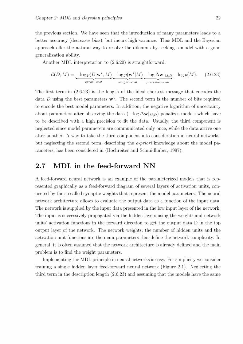
Implementing the MDL principle in neural networks is easy. For simplicity we consider
training a single hidden layer feed-forward neural network (Figure 2.1). Neglecting the
third term in the description length (2.6.23) and assuming that the models have the same
Chapter 2: MDL and Bayesian principles 23
Supervised feed-forward network
w - hidden weights
representation - A
Hidden
Input - X
W - top weights
Output
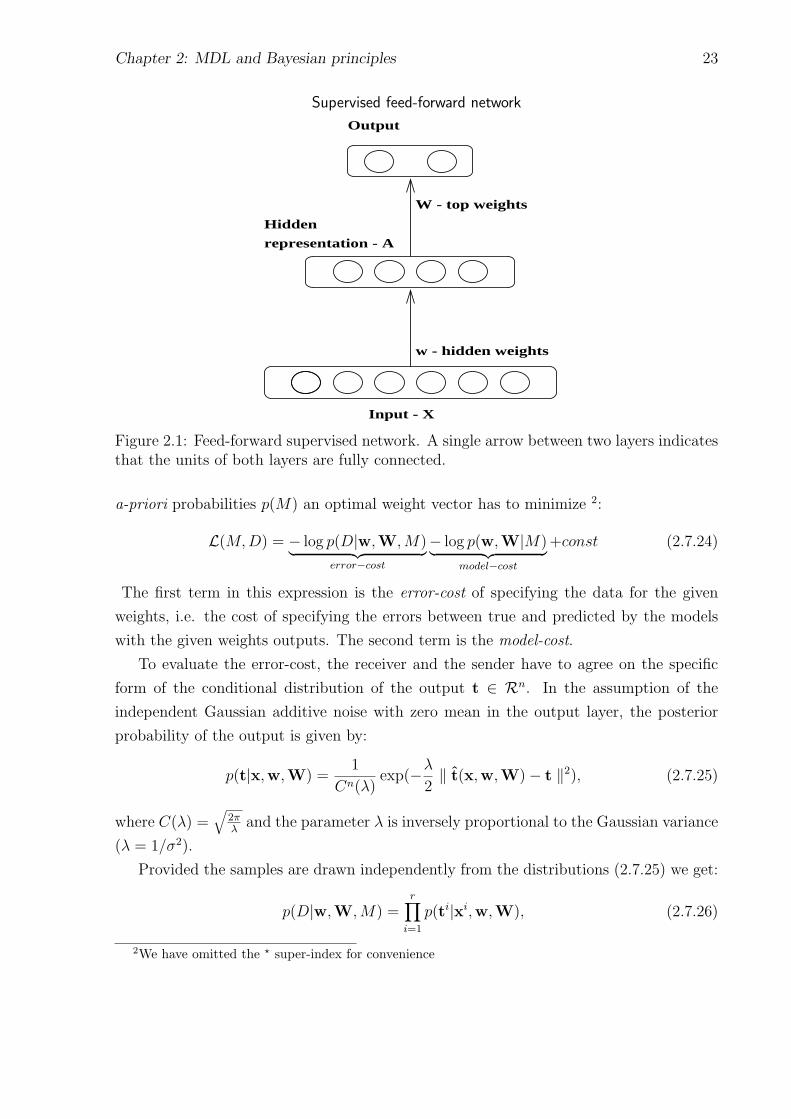
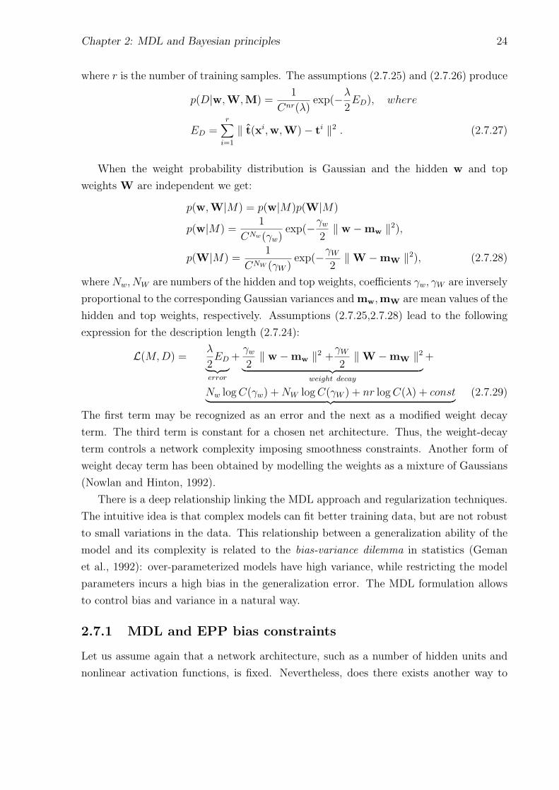
Figure 2.1: Feed-forward supervised network. A single arrow between two layers indicatesthat the units of both layers are fully connected.
a-priori probabilities p(M) an optimal weight vector has to minimize 2:
L(M,D) = − log p(D|w,W,M)︸ ︷︷ ︸error−cost
− log p(w,W|M)︸ ︷︷ ︸model−cost
+const (2.7.24)
The first term in this expression is the error-cost of specifying the data for the given
weights, i.e. the cost of specifying the errors between true and predicted by the models
with the given weights outputs. The second term is the model-cost.
To evaluate the error-cost, the receiver and the sender have to agree on the specific
form of the conditional distribution of the output t ∈ Rn. In the assumption of the
independent Gaussian additive noise with zero mean in the output layer, the posterior
probability of the output is given by:
p(t|x,w,W) =1
Cn(λ)exp(−λ
2‖ t(x,w,W)− t ‖2), (2.7.25)
where C(λ) =√
2πλ
and the parameter λ is inversely proportional to the Gaussian variance
(λ = 1/σ2).
Provided the samples are drawn independently from the distributions (2.7.25) we get:
p(D|w,W,M) =r∏
i=1
p(ti|xi,w,W), (2.7.26)
2We have omitted the ? super-index for convenience
Chapter 2: MDL and Bayesian principles 24
where r is the number of training samples. The assumptions (2.7.25) and (2.7.26) produce
p(D|w,W,M) =1
Cnr(λ)exp(−λ
2ED), where
ED =r∑
i=1
‖ t(xi,w,W)− ti ‖2 . (2.7.27)
When the weight probability distribution is Gaussian and the hidden w and top
weights W are independent we get:
p(w,W|M) = p(w|M)p(W|M)
p(w|M) =1
CNw(γw)exp(−γw
2‖ w −mw ‖2),
p(W|M) =1
CNW (γW )exp(−γW
2‖W −mW ‖2), (2.7.28)
where Nw, NW are numbers of the hidden and top weights, coefficients γw, γW are inversely
proportional to the corresponding Gaussian variances and mw,mW are mean values of the
hidden and top weights, respectively. Assumptions (2.7.25,2.7.28) lead to the following
expression for the description length (2.7.24):
L(M,D) =λ
2ED
︸ ︷︷ ︸error
+γw2‖ w −mw ‖2 +
γW2‖W −mW ‖2
︸ ︷︷ ︸weight decay
+
Nw logC(γw) +NW logC(γW ) + nr logC(λ) + const︸ ︷︷ ︸ (2.7.29)
The first term may be recognized as an error and the next as a modified weight decay
term. The third term is constant for a chosen net architecture. Thus, the weight-decay
term controls a network complexity imposing smoothness constraints. Another form of
weight decay term has been obtained by modelling the weights as a mixture of Gaussians
(Nowlan and Hinton, 1992).
There is a deep relationship linking the MDL approach and regularization techniques.
The intuitive idea is that complex models can fit better training data, but are not robust
to small variations in the data. This relationship between a generalization ability of the
model and its complexity is related to the bias-variance dilemma in statistics (Geman
et al., 1992): over-parameterized models have high variance, while restricting the model
parameters incurs a high bias in the generalization error. The MDL formulation allows
to control bias and variance in a natural way.
2.7.1 MDL and EPP bias constraints
Let us assume again that a network architecture, such as a number of hidden units and
nonlinear activation functions, is fixed. Nevertheless, does there exists another way to
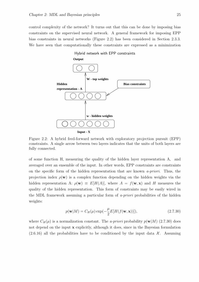
Chapter 2: MDL and Bayesian principles 25
control complexity of the network? It turns out that this can be done by imposing bias
constraints on the supervised neural network. A general framework for imposing EPP
bias constraints in neural networks (Figure 2.2) has been considered in Section 2.3.3.
We have seen that computationally these constraints are expressed as a minimization
Hybrid network with EPP constraints
w - hidden weights
representation - A
Hidden
Input - X
W - top weights
Bias constraints
Output
Figure 2.2: A hybrid feed-forward network with exploratory projection pursuit (EPP)constraints. A single arrow between two layers indicates that the units of both layers arefully connected.
of some function H, measuring the quality of the hidden layer representation A, and
averaged over an ensemble of the input. In other words, EPP constraints are constraints
on the specific form of the hidden representation that are known a-priori. Thus, the
projection index ρ(w) is a complex function depending on the hidden weights via the
hidden representation A: ρ(w) ≡ E[H(A)], where A = f(w,x) and H measures the
quality of the hidden representation. This form of constraints may be easily wired in
the MDL framework assuming a particular form of a-priori probabilities of the hidden
weights:
p(w|M) = CH(µ) exp(−µ2E[H(f(w,x))]), (2.7.30)
where CH(µ) is a normalization constant. The a-priori probability p(w|M) (2.7.30) does
not depend on the input x explicitly, although it does, since in the Bayesian formulation
(2.6.16) all the probabilities have to be conditioned by the input data X . Assuming

Chapter 2: MDL and Bayesian principles 26
independence of the hidden and top weights, we get:
L(M,D) =1
2λED
︸ ︷︷ ︸error−cost
+1
2µE[H(A)]
︸ ︷︷ ︸representation−cost
− log p(W|M)︸ ︷︷ ︸weight−cost
+const. (2.7.31)
The expression for the description length (2.7.31) gives a deeper level of description to
the data communication and is close (though not equivalent) to Zemel’s interpretation of
MDL (Zemel, 1993).
In Zemel’s interpretation one gets a more realistic interpretation of the communication
game, where a real communication takes place between the hidden layer with internal
representation A and the top layer. The receiver requires three items in order to be able
to recover the desired output:
1. The set of activities A of the representation units; these are codes that nets assign to
each training input sample. Encoding activities of the representation (hidden) units
avoids communication of the hidden weights and does not require the knowledge of
the input data X . However, the sender and the receiver have to agree on the a-priori
distribution of the internal representation. This part of the message corresponds to
the representation-cost.
2. The set of hidden-to-output weights W . This part of the message is represented by
the weight-cost.
3. Reconstruction error, which is a misfit between desired and predicted outputs. This
part of the message is represented by the reconstruction or the error-cost. In order
to evaluate the latter, the sender and receiver have to agree on the probability of
the desired output of the network given its actual output.
Usually, the weight-cost, i.e. the number of bits required to communicate the hidden-
to-top weights, is not taken into account, since it has to be communicated only once,
while representation-cost and error-cost have to be sent for every sample. Thus, the main
communication tradeoff takes place between representation and error costs. Reducing
dimensionality of the data in the hidden layer, i.e. compressing the data, a shorter
description is obtained, but at the same time the errors are larger. The MDL principle is
a tool for achieving a good data representation that is compact and accurate.
We see that similar to Zemel’s interpretation of MDL, imposing EPP constraints leads
to the description length (Eq. 2.7.31) that consists of three parts. It requires the same
agreement on probabilities of hidden representation and errors between the sender and
receiver as described above. However, the representation cost in (Eq. 2.7.31) is taken only

Chapter 2: MDL and Bayesian principles 27
once for all samples, while in Zemel’s interpretation it is permanent and is assigned to each
training input sample. When the number of input patterns is infinite, the representation
cost induced by EPP constraints is negligible. Thus, in a manner similar to supervised
learning, EPP constraints lead to a model in which model cost vanishes as the number of
input patterns becomes infinite.
We postpone the consideration of the hybrid autoencoder network with reconstruction
constraints and its MDL interpretation to the next section, where reconstruction task and
its application are considered.

Chapter 2: Regularization problem 28
2.8 Appendix to Chapter 2: Regularization problem
Regularization may be expressed as a minimization problem with a goal function that is
a penalized cost function:
Eλ = E + λΩ(f ,w), E =∑
i
‖ yi − f(xi, ω) ‖2 .
A large value of the regularization parameter λ leads to a network with a large bias
(unless the regularization term captures the underlying structure of the data), while a
small value reduces bias but increases variance. Then the regularization task is to find
an optimal parameter λ? and corresponding model parameters ωλ? providing the minimal
generalization error:
Eλ? = E[‖ y − f(x, ωλ?) ‖2].
This task is computationally very expensive.
Split-sample validation and hold-out method The simplest way to find the regu-
larization parameter is to use split-sample validation. This process includes the following
steps for each tested value of the regularization parameter λ (this process is common for
the choice of the other regularization parameters, such as the number of hidden units, a
choice of the early time stopping moment, etc.):
• A random data is split into a training and validation set. Often 2/3 of the data is
used for training and 1/3 for testing.
• The training set is used for estimation of the predictor parameters by minimizing
Eλ.
• The validation set is used to test a prediction error (E). The validation set must
not be used in any way during training.
• The predictor with the smallest prediction error corresponds to the optimal regu-
larization parameter λ.
The generalization error of the best predictor is in general too optimistic. The prediction
error on a third separately kept data set, called the test set is more realistic and is
often reported as the result of the predictor accuracy. This method is called the hold-out
method.
The disadvantage of the split-sample validation and hold-out method is that they
reduce the amount of data available for both training and validation. Two methods that

Chapter 2: Regularization problem 29
overcome this drawback are cross-validation and bootstrapping (Efron and Tibshirani,
1993; Bishop, 1995a).
Cross-validation In k-fold cross-validation, the data is divided into k subsets of (ap-
proximately) equal size. A network is trained k times, each time leaving out one of the
subsets from the training set and using the omitted subset as a validation set to compute
an error. If k equals the sample set size, this is called “leave-one-out” cross-validation.
“Leave-v-out” is a more elaborate and expensive version of cross-validation that involves
leaving out all possible subsets of v cases. A generalization error is then measured as an
average performance over all possible validation tests. Cross-validation is an improvement
on split-sample validation.
Bootstrapping In many cases, bootstrap seems to be better than cross-validation
(Efron and Tibshirani, 1993). In the simplest form of bootstrapping, the training data is
bootstrapped, instead of repeatedly analyzing subsets of the data as in cross-validation.
Given a data set of size n, a bootstrap sample is created by sampling n instances uni-
formly from the data with replacement. Then the probability of the instance to remain in
the test set is (1− 1/n)n ≈ e−1 ≈ 0.368; and to be in the training data is 0.632. Given a
number b of bootstrap samples, the average performance is evaluated as a weighted sums
of the training (E trainingi ) and testing (E testingi ) errors:
E =1
b
b∑
i=1
(0.632E trainingi + 0.368E testingi ) (2.8.32)
Usually the number of recommended bootstrap samples is between 200 − 2000 (Kohavi,
1995).
Cross-validation and bootstrapping require many runs that may be computationally
prohibitive, especially for the most interesting perception tasks, when the input dimension-
ality is very high. Both cross-validation and bootstrapping work well for continuous error
functions, such as the mean squared error, but it may perform poorly for non-continuous
error functions, such as the misclassification rate.

Chapter 3
Imposing bias via reconstructionconstraints
3.1 Introduction
Reconstruction is one of the important tasks of the complex visual processing. It is
a process of reproducing the input via some reasonably well chosen model. It is com-
monly assumed that there is a compression via a bottleneck model and thus, the input
is reproduced from a reduced internal representation. The oldest and widely spread re-
construction method is Principal Component Analysis (PCA). PCA is an optimal linear
compression, that is based on minimization of the mean squared error between input and
its reconstruction. A simple generalization of PCA, in the nonlinear case, is a nonlinear
autoencoder. Below, we present both these models and discuss their relationship to the
MDL principle.
We proceed then with a more general notion of reconstruction via a generative model
and reexamine diverse applications of the reconstruction models. Finally, we introduce a
novel method that uses reconstruction as a bias constraint to a supervised classification
task.
3.1.1 Principal Component Analysis (PCA)
PCA is widely used in multivariate analysis (Duda and Hart, 1973). PCA, also known as
the Karhunen-Loeve transformation (Oja, 1982; Fukunaga, 1990), is a process of mapping
the original data into a more efficient representation, using an orthonormal linear trans-
formation that minimizes the mean squared error between the data and its reconstructed
version.
It is well-known that the optimal orthogonal basis of the data space is formed by the
eigenvectors of the covariance matrix of the data. New data representation is obtained
30
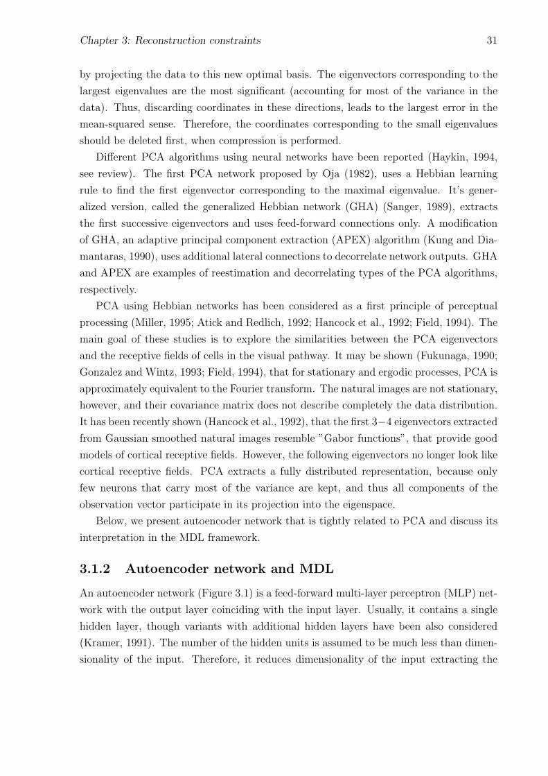
Chapter 3: Reconstruction constraints 31
by projecting the data to this new optimal basis. The eigenvectors corresponding to the
largest eigenvalues are the most significant (accounting for most of the variance in the
data). Thus, discarding coordinates in these directions, leads to the largest error in the
mean-squared sense. Therefore, the coordinates corresponding to the small eigenvalues
should be deleted first, when compression is performed.
Different PCA algorithms using neural networks have been reported (Haykin, 1994,
see review). The first PCA network proposed by Oja (1982), uses a Hebbian learning
rule to find the first eigenvector corresponding to the maximal eigenvalue. It’s gener-
alized version, called the generalized Hebbian network (GHA) (Sanger, 1989), extracts
the first successive eigenvectors and uses feed-forward connections only. A modification
of GHA, an adaptive principal component extraction (APEX) algorithm (Kung and Dia-
mantaras, 1990), uses additional lateral connections to decorrelate network outputs. GHA
and APEX are examples of reestimation and decorrelating types of the PCA algorithms,
respectively.
PCA using Hebbian networks has been considered as a first principle of perceptual
processing (Miller, 1995; Atick and Redlich, 1992; Hancock et al., 1992; Field, 1994). The
main goal of these studies is to explore the similarities between the PCA eigenvectors
and the receptive fields of cells in the visual pathway. It may be shown (Fukunaga, 1990;
Gonzalez and Wintz, 1993; Field, 1994), that for stationary and ergodic processes, PCA is
approximately equivalent to the Fourier transform. The natural images are not stationary,
however, and their covariance matrix does not describe completely the data distribution.
It has been recently shown (Hancock et al., 1992), that the first 3−4 eigenvectors extracted
from Gaussian smoothed natural images resemble ”Gabor functions”, that provide good
models of cortical receptive fields. However, the following eigenvectors no longer look like
cortical receptive fields. PCA extracts a fully distributed representation, because only
few neurons that carry most of the variance are kept, and thus all components of the
observation vector participate in its projection into the eigenspace.
Below, we present autoencoder network that is tightly related to PCA and discuss its
interpretation in the MDL framework.
3.1.2 Autoencoder network and MDL
An autoencoder network (Figure 3.1) is a feed-forward multi-layer perceptron (MLP) net-
work with the output layer coinciding with the input layer. Usually, it contains a single
hidden layer, though variants with additional hidden layers have been also considered
(Kramer, 1991). The number of the hidden units is assumed to be much less than dimen-
sionality of the input. Therefore, it reduces dimensionality of the input extracting the

Chapter 3: Reconstruction constraints 32
Autoencoder network architecture
w - hidden weights
W - hidden-to-top weights
Figure 3.1: Reconstruction of the inputs is done from the hidden layer representation.
so-called internal representation in the hidden layer.
The autoencoder network has a natural interpretation in the MDL framework (Hinton
and Zemel, 1994). It discovers an efficient way to communicate data to a receiver. A
sender uses a set of input-to-hidden weights and, in general, non-linear activation functions
to convert the input into a compact hidden representation. This representation has to
be communicated to the receiver along with the reconstruction errors and hidden-to-top
weights. Knowing the hidden-to-top weights the receiver reconstructs the input from this
abstract representation and communicated errors.
From Eq. 2.7.24 the description length is composed of the error-cost and the model-
cost. Assuming that the errors are encoded using a zero-mean Gaussian with the same
predetermined variance for each output unit, the error-cost is given by the sum of the
squared errors. Since in the autoencoder the hidden units are always active, the model cost
may be approximated by the size of the hidden layer. Often, the model cost is ignored,
and the MDL principle leads to a simple minimization of the sum of squared errors
via a network with a bottleneck structure. Thus, the autoencoder learns the compact
representation of the input. In addition, the bottleneck structure forces the network to
learn prominent features of the input distribution which are useful for generalization. The
network is robust to noise and may be used for pattern completion, when part of the input
is corrupted or absent.
A linear one-hidden layer autoencoder is closely related to PCA, since its hidden
weights span the same subspace as found by principal eigenvectors (Bourlard and Kamp,
1988). However, contrary to PCA, the hidden weights are not forced to be orthogo-
nal and do not coincide with the hidden-to-top weights. The analytical solution of the

Chapter 3: Reconstruction constraints 33
optimization problem imposed by the linear autoencoder is given by:
W = UT−1, w = TUt (3.1.1)
where T ∈ Rp×p is an arbitrary nonsingular scaling matrix; U ∈ Rn×p (p ≤ n) is a
matrix of the principal eigenvectors stacked by columns; W and w are hidden-to-top
and hidden weights respectively; n and p are the number of units in the input and hidden
layers respectively. However, since learning in the autoencoder relies on a gradient descent
technique it can get trapped in local minima.
In the nonlinear case, Bourlard and Kamp claim that nonlinear and linear autoen-
coders are equivalent, since when the norm of the scaling matrix T is infinitely small,
sigmoidal activation functions can be approximated arbitrary close by linear activation
functions. However, their proof is valid only from the reconstruction error minimization
viewpoint, and not the extracted internal representation context. Their analysis does
not take into account a convergence issue. Indeed, to make nonlinear and linear autoen-
coder solutions arbitrarily close, the norm of the matrix T has to be arbitrarily small (for
example, by introducing some scaling parameter ε → 0). While ε is positive the linear
autoencoder hidden weights span the same space as the principal eigenvectors, but at
the same time there is a difference between hidden weights extracted by the linear and
nonlinear autoencoders. This difference disappears only for ε = 0, when the matrix T
becomes singular. Thus, it is not obvious that the hidden weights obtained in the limit
of this convergence span the space extracted by the principal eigenvectors.
It has been recently shown, that when the data is whitened (i.e. the data covariance
matrix is unit and spherical) and non-linear activation functions are adjusted properly, the
autoencoder is able to extract the independent components (Oja, 1995a) (i.e. responses
of different hidden neurons are independent, see also Chapter 4), while the PCA solution
is not well defined. Thus, the non-linear autoencoder can be made sensitive to higher
order statistics, while PCA is sensitive to the second order statistics of the data.
The presence of the proper nonlinearities in the autoencoder allows to extract sparse
representation, while PCA forms distributed representation. In the distributed represen-
tation, all the hidden units participate in the pattern encoding, while in the sparse, only
a few are active, which are responsible for the presence of some specific features in the
pattern. PCA forms the distributed representation, since only few neurons which carry
most of the variance are kept for data reconstruction and they are active for all patterns.
Other variants of autoencoders that encourage sparse hidden representations have
been proposed by Zemel (1993). The code-cost of the sparse representation is small, even
when the number of hidden units is large. Thus, though these autoencoders are trained
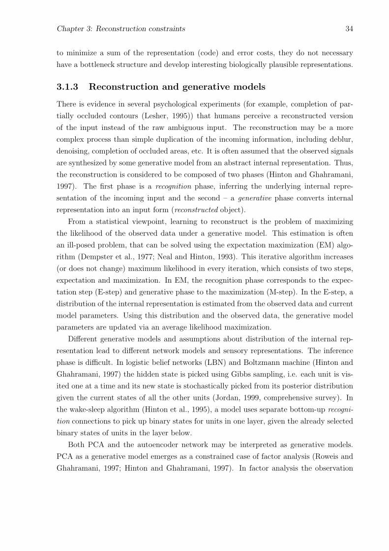
Chapter 3: Reconstruction constraints 34
to minimize a sum of the representation (code) and error costs, they do not necessary
have a bottleneck structure and develop interesting biologically plausible representations.
3.1.3 Reconstruction and generative models
There is evidence in several psychological experiments (for example, completion of par-
tially occluded contours (Lesher, 1995)) that humans perceive a reconstructed version
of the input instead of the raw ambiguous input. The reconstruction may be a more
complex process than simple duplication of the incoming information, including deblur,
denoising, completion of occluded areas, etc. It is often assumed that the observed signals
are synthesized by some generative model from an abstract internal representation. Thus,
the reconstruction is considered to be composed of two phases (Hinton and Ghahramani,
1997). The first phase is a recognition phase, inferring the underlying internal repre-
sentation of the incoming input and the second – a generative phase converts internal
representation into an input form (reconstructed object).
From a statistical viewpoint, learning to reconstruct is the problem of maximizing
the likelihood of the observed data under a generative model. This estimation is often
an ill-posed problem, that can be solved using the expectation maximization (EM) algo-
rithm (Dempster et al., 1977; Neal and Hinton, 1993). This iterative algorithm increases
(or does not change) maximum likelihood in every iteration, which consists of two steps,
expectation and maximization. In EM, the recognition phase corresponds to the expec-
tation step (E-step) and generative phase to the maximization (M-step). In the E-step, a
distribution of the internal representation is estimated from the observed data and current
model parameters. Using this distribution and the observed data, the generative model
parameters are updated via an average likelihood maximization.
Different generative models and assumptions about distribution of the internal rep-
resentation lead to different network models and sensory representations. The inference
phase is difficult. In logistic belief networks (LBN) and Boltzmann machine (Hinton and
Ghahramani, 1997) the hidden state is picked using Gibbs sampling, i.e. each unit is vis-
ited one at a time and its new state is stochastically picked from its posterior distribution
given the current states of all the other units (Jordan, 1999, comprehensive survey). In
the wake-sleep algorithm (Hinton et al., 1995), a model uses separate bottom-up recogni-
tion connections to pick up binary states for units in one layer, given the already selected
binary states of units in the layer below.
Both PCA and the autoencoder network may be interpreted as generative models.
PCA as a generative model emerges as a constrained case of factor analysis (Roweis and
Ghahramani, 1997; Hinton and Ghahramani, 1997). In factor analysis the observation

Chapter 3: Reconstruction constraints 35
is a linear transformation of the hidden variables, corrupted with an additive sensory
noise that is Gaussian. The linear transformation is realized via a matrix of the gener-
ative weight vectors. Each generative weight vector connects hidden variables with the
corresponding observation variable. Hidden variables are referred to as factors and are
assumed to be Gaussian. PCA is obtained when the covariance matrix of the sensory
noise is assumed to be a scaled identity matrix εI, with the infinitesimal scaling factor
ε→ 0. In this limiting case, the posterior distribution of the hidden variables shrinks to a
single point, i.e. given the observation, the hidden representation becomes non random.
In PCA the generative weight vectors are forced to be orthogonal, that leads to a simple
recognition of the deterministic hidden representation as a linear transformation with the
matrix of the recognition weight vectors equal to the transpose of the generative weight
matrix.
Interpretation of PCA as a generative model disregards the order of the hidden vari-
ables, but allows the use of EM for the extraction of eigenvectors (Roweis, 1997). This
method is especially efficient for high dimensional data, where a covariance matrix is not
full rank and has a large size that makes the simple diagonalization of the covariance
matrix computationally difficult.
The transformation from the input to the hidden layer in the autoencoder net is
associated with the recognition phase and from the hidden layer to the output as the
generative phase. Therefore, the hidden weights emerge as recognition weights and the
hidden-to-top weights as generative weights.
3.1.4 Classification via reconstruction
As we have shown above, an implicit reconstruction goal is to find a meaningful internal
representation of the data that can be obviously used for data compression and commu-
nication. Interpreted as a set of good features, it may be applied for further processing
and learning. This usage is not absolutely apparent, since during feature extraction some
information is lost. Below, we consider some examples of using internal representations
extracted via reconstruction for recognition.
PCA for classification PCA was first used as a means of preprocessing for subsequent
face recognition in (Kirby and Sirovich, 1990; Turk and Pentland, 1991). Later PCA was
used for a man-made object recognition and pose estimation (Murase and Nayar, 1993).
PCA proceeds by scanning and representing images as points of a high dimensional
space with the dimension equal to the number of image pixels. The eigenvectors of the
data covariance matrix represented as images are called the eigenpictures. The first large
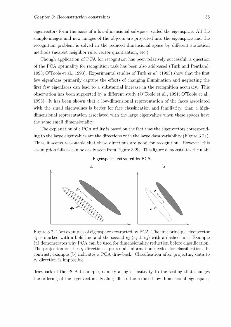
Chapter 3: Reconstruction constraints 36
eigenvectors form the basis of a low-dimensional subspace, called the eigenspace. All the
sample-images and new images of the objects are projected into the eigenspace and the
recognition problem is solved in the reduced dimensional space by different statistical
methods (nearest neighbor rule, vector quantization, etc.).
Though application of PCA for recognition has been relatively successful, a question
of the PCA optimality for recognition task has been also addressed (Turk and Pentland,
1993; O’Toole et al., 1993). Experimental studies of Turk et al. (1993) show that the first
few eigenfaces primarily capture the effects of changing illumination and neglecting the
first few eigenfaces can lead to a substantial increase in the recognition accuracy. This
observation has been supported by a different study (O’Toole et al., 1991; O’Toole et al.,
1993). It has been shown that a low-dimensional representation of the faces associated
with the small eigenvalues is better for face classification and familiarity, than a high-
dimensional representation associated with the large eigenvalues when these spaces have
the same small dimensionality.
The explanation of a PCA utility is based on the fact that the eigenvectors correspond-
ing to the large eigenvalues are the directions with the large data variability (Figure 3.2a).
Thus, it seems reasonable that these directions are good for recognition. However, this
assumption fails as can be easily seen from Figure 3.2b. This figure demonstrates the main
Eigenspaces extracted by PCA
a b
e2
e1
e2
e1
Figure 3.2: Two examples of eigenspaces extracted by PCA. The first principle eigenvectore1 is marked with a bold line and the second e2 (e1 ⊥ e2) with a dashed line. Example(a) demonstrates why PCA can be used for dimensionality reduction before classification.The projection on the e1 direction captures all information needed for classification. Incontrast, example (b) indicates a PCA drawback. Classification after projecting data toe1 direction is impossible.
drawback of the PCA technique, namely a high sensitivity to the scaling that changes
the ordering of the eigenvectors. Scaling affects the reduced low-dimensional eigenspace,

Chapter 3: Reconstruction constraints 37
extracted by PCA and being optimal for reconstruction it may be inappropriate for recog-
nition. When the data is whitened, PCA is not clear at all, since all orthogonal systems
are equivalent from a PCA viewpoint.
Autoencoder network The autoencoder networks have been successfully used not
only for compression (Mougeot et al., 1991; Cottrell et al., 1987), but for classification as
well (Elman and Zipser, 1988; Japkowicz et al., 1995; Schwenk and Milgram, 1995). In
these works, a classification process is considered to consist of two phases. In the first
phase several autoencoders are trained. Each autoencoder is trained separately on the
samples of the corresponding class. The second phase is heuristic and is based on the idea
that the reconstruction error is, in general, much lower for examples of the learned class
than for the other ones.
In (Japkowicz et al., 1995) classification is constrained to a two-class discrimination
task that is replaced by a dual task of familiarity with a concept. In the first phase, the
single autoencoder is trained on the conceptual examples solely. In the second phase, the
conceptual examples or two classes examples are used to estimate the decision threshold
for a reconstruction error (the sum of squared errors) between input and output. If
the reconstruction error is smaller than the decision threshold, the instance is classified
as conceptual, if larger it is classified as counter-conceptual. Similarly, in (Elman and
Zipser, 1988) the autoencoder is trained on segmented sounds that allows to segment a
continuous speech on the base of the mean squared error.
In (Schwenk and Milgram, 1995) the basic idea is to use one autoencoder for each
class and to train it only with examples of the corresponding class. In contrast with the
usual autoencoder, a tangent distance is used instead of the squared reconstruction error.
This tangent distance allows to incorporate a high-level knowledge about typical input
transformation. Classification is done using the reconstruction errors of the autoencoders
as discriminant functions.
“Wake-sleep” network Another example of classification based on the reconstruction
has been proposed via the “wake-sleep” network (Hinton et al., 1995). Similarly to au-
toencoders, each “wake-sleep” network is trained separately on different examples of the
same digit. Classification is done by observing which of the networks provides the most
economical description of the data.

Chapter 3: Reconstruction constraints 38
3.1.5 Other applications of reconstruction
Reconstruction via a modified autoencoder has been used for input reconstruction relia-
bility estimation (IRRE) for autonomous car navigation (Pomerleau, 1993). In IRRE a
connectionist network is trained simultaneously to produce the correct steering response
for a car navigation and to reconstruct the input image in the mean squared error sense.
After learning, the reliability measure which is a correlation between the input and its
reconstructed image is evaluated. This reliability measure may be used to control vehicle
speed and its location in the a priori known confusing situations. Another application
of IRRE is by integrating the outputs of multiple networks trained for different driving
situations, i.e. the network that has the best reliability has to be used for a navigation
task.
Another related recurrent network has been used for autonomous vehicle navigation
(Baluja and Pomerleau, 1995). Baluja et al. use prediction of the next future input image
as a related task to the navigation task, i.e. the MLP network is learned to predict an
input image and to produce a right steering response simultaneously. Computationally,
the hidden weights are updated based on the navigation task only, but from the obtained
hidden activities the network is trained to predict. Recursion has a place by propagating
the predicted image back to the input layer for refining the next input image via noise
and unpredicted object elimination.
A similar to IRRE connectionist network has been proposed as a hippocampal model
(Gluck and Myers, 1993). This model assumes that the hippocampal region develops
stimulus internal representation that enhances the discrimination of predictive cues while
compressing the representation of redundant cues.
3.2 Imposing reconstruction constraints
3.2.1 Reconstruction as a bias imposing mechanism
We have shown above that the reconstruction task is related to the classification task
and two main approaches to classification via reconstruction take place. The first ap-
proach offers the use of a common hidden representation obtained for all data as a pre-
processing step for the following learning (Kirby and Sirovich, 1990; Murase and Nayar,
1993; Moghaddam and Pentland., 1994). In the second approach (Japkowicz et al., 1995;
Schwenk and Milgram, 1995; Hinton et al., 1995), reconstruction (generative) networks
are used to extract the underlying structure of the data drawn from the same class.
The assumption is that an example drawn from another class does not share the already
Chapter 3: Reconstruction constraints 39
learned structure and produces a high description length. Thus, the description length
may be used as a discriminant function.
Though these approaches have been relatively successful, there are cases when they are
not appropriate. For example, when the samples belonging to the same class have multi-
modal distribution, or the classes are very similar, the second approach is not obvious.
As we have shown in Section 3.1.4, PCA is very sensitive to data scaling.
This consideration favors the view that each perceptual task needs data preprocessing
that can not be obtained based only on the other related task. Contrary to the considered
above approaches, we propose to use reconstruction realized via a modified autoencoder as
a bias-imposing mechanism in the feed-forward networks for improving the classification
task. An intuitive way to conceive the idea of imposing reconstruction as a proper bias
constraint for classification is via the multi-task learning (MTL) approach (2.3.3). As
has been shown above both recognition and reconstruction are related but different tasks
of visual processing. In some cases, they were also replaced by one another. Secondly,
it has been experimentally shown (Elman and Zipser, 1988; Cottrell et al., 1987), that
reconstruction via an autoencoder extracts a valuable internal representation. Thus, it is
reasonable that hidden representation that relies on recognition and reconstruction tasks
can improve the generalization performance of classification. This assumes that such
hidden representation has to capture some prominent (recognition) features of the data,
while keeping most important information needed for reconstruction.
As an illustration, let us assume that we want to classify between two individuals and
suppose that one of them has some prominent features in the training images (glasses, hair
style, moustache, beard and so on), then it seems plausible that recognition will exhibit
a tendency to process these corresponding areas of the face and all the other information
will be redundant for the recognition goal. However, these features may be absent or
appear rarely in new images of this person, thus failure in the testing phase is likely. In
contrast, the addition of the reconstruction task during training of the system, forces the
system to extract other features which may not be so useful for recognition of the original
training images, but may be of use with the novel test set. This motivates our suggestion
to add reconstruction constraints during learning of the classification task.
Similar approach has been proposed in (Gluck and Myers, 1993) to model a hip-
pocampus function. It is assumed that one of the roles of the hippocampus is to extract a
common recognition/reconstruction internal representation of the input stimulus. Though
conceptually our work is close to this model we have remarkable differences that are elu-
cidated later on. Below, we present a hybrid classification/reconstruction network.
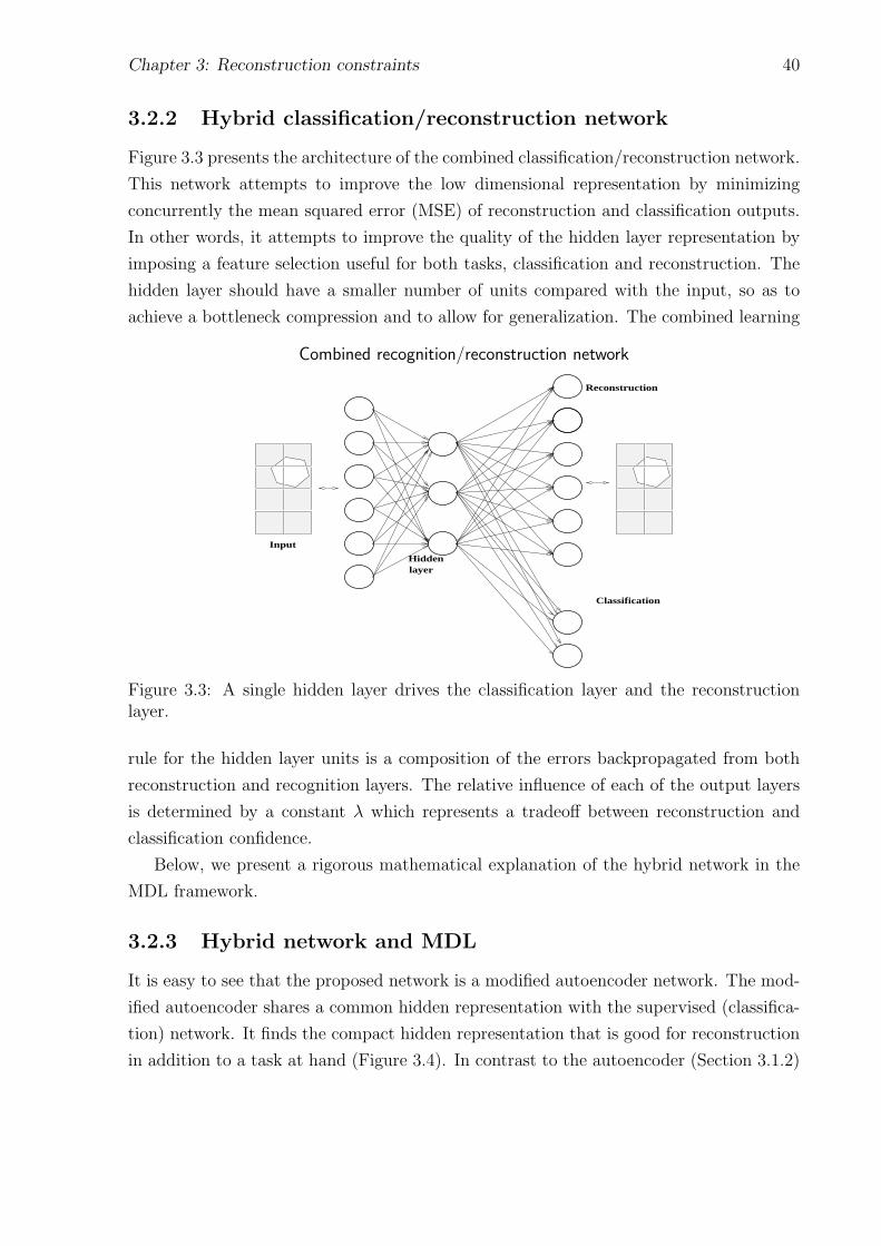
Chapter 3: Reconstruction constraints 40
3.2.2 Hybrid classification/reconstruction network
Figure 3.3 presents the architecture of the combined classification/reconstruction network.
This network attempts to improve the low dimensional representation by minimizing
concurrently the mean squared error (MSE) of reconstruction and classification outputs.
In other words, it attempts to improve the quality of the hidden layer representation by
imposing a feature selection useful for both tasks, classification and reconstruction. The
hidden layer should have a smaller number of units compared with the input, so as to
achieve a bottleneck compression and to allow for generalization. The combined learning
Combined recognition/reconstruction network
Classification
Reconstruction
Hiddenlayer
Input
Figure 3.3: A single hidden layer drives the classification layer and the reconstructionlayer.
rule for the hidden layer units is a composition of the errors backpropagated from both
reconstruction and recognition layers. The relative influence of each of the output layers
is determined by a constant λ which represents a tradeoff between reconstruction and
classification confidence.
Below, we present a rigorous mathematical explanation of the hybrid network in the
MDL framework.
3.2.3 Hybrid network and MDL
It is easy to see that the proposed network is a modified autoencoder network. The mod-
ified autoencoder shares a common hidden representation with the supervised (classifica-
tion) network. It finds the compact hidden representation that is good for reconstruction
in addition to a task at hand (Figure 3.4). In contrast to the autoencoder (Section 3.1.2)

Chapter 3: Reconstruction constraints 41
Hybrid network with reconstruction and EPP constraints
w - hidden weights
representation - AHidden
W W
Reconstruction
hidden-to-top
weights Bias constraints
Input - X
Output
12
Figure 3.4: The hidden layer drives the reconstruction and classification output. Inaddition, the search of another statistical structure in the data is made.
and supervised feed-forward network (Section 2.7), the hybrid network is associated with
a different communication game, in which the sender uses a compact internal representa-
tion to communicate both the observed data and the corresponding desired output (for
example, class labels of the images). Since this internal representation has to encode
efficiently both the observed data and corresponding output, a cost for communicating
the input data X has to be involved in the description length (2.7.24), yielding:
L(M,D,X ) = − log p(D,X|w,W1,W2,M)− log p(w,W1,W2|M) + const.
Assuming that given the input and the net weights, conditional probabilities of the recon-
struction and supervised outputs are independent and Gaussian, we get similar to (2.7.29)
the expression for the description length:
L(M,D,X ) =1
2(λ1ED + λ2EX )− log p(w,W1,W2|M) +
r1d logC(λ1) + r2n logC(λ2) + const. (3.2.2)
In expression for the description length (3.2.2), λ1 and λ2 are inversely proportional to
the variances of the specific task and reconstruction outputs respectively; ED and EX are
sums of the squared errors of the supervised task and reconstruction outputs, respectively;
r1, r2 are numbers of training samples for reconstruction and specific tasks.
Assuming the same a-priori probability for the hidden weights as in (2.7.30), the entire

Chapter 3: Reconstruction constraints 42
description length may be simplified to:
L(M,D,X ) =1
2(λ1ED + λ2EX + µE[H(w,x)])
︸ ︷︷ ︸(1)
+
r1d logC(λ1) + r2n logC(λ2) + logCH(µ) + const︸ ︷︷ ︸(2)
. (3.2.3)
In general, the numbers of training samples for reconstruction (r1) and specific (r2)
tasks may be different, which seems to be a common situation in a real-world learning.
In the limit, when we do not have enough information provided by supervised learning,
internal representation is constructed based on the unsupervised learning only.
Since, in our consideration, parameters λ1, λ2, µ are assumed to be fixed, the second
part of the description length (3.2.3) is a constant and the description length may be
rewritten as:
L(M,D,X ) = 12(λ1ED + λ2EX + µE[H(w,x)]) + Const (3.2.4)
Therefore, when one is interested in both tasks, two scaled sum-square errors ED and EXpresent the error cost and the third term µE[H(w,x)] is the model-cost or representation-
cost. This interpretation of the hybrid network in the MDL framework is not single.
Indeed, an interpretation depends on a way to look at the hybrid network.
When one is mainly interested in the reconstruction via bottleneck hybrid structure,
the task may be formulated as a compression problem. This compression has benefits
compared to a conventional autoencoder, since it admits not only a good reconstruction
of the data, but a successful handling on the specific task, such as classification, for
example. In this statement, the reconstruction error EX is recognized as the error cost
and the scaled classification error and third term as the model-cost.
The third and the last interpretation is produced when one is mainly interested in
the specific task (for example, classification or control tasks). In this case, the specific
error ED is recognized as the error cost and the scaled reconstruction error and third term
as the model-cost. This interpretation gives the rigorous mathematical way for imposing
reconstruction and other unsupervised types of constraints in the supervised network.
Below, based on this last interpretation, we explain why the hybrid network may be
better than the conventional classification feed-forward network. Let us consider two
different principal melodies. Suppose that the first is embellished with specific tones,
however, the second is not arranged at all. Hearing these two melodies, arranged and not,
many times, one can decide that these specific tones are enough for recognizing, which
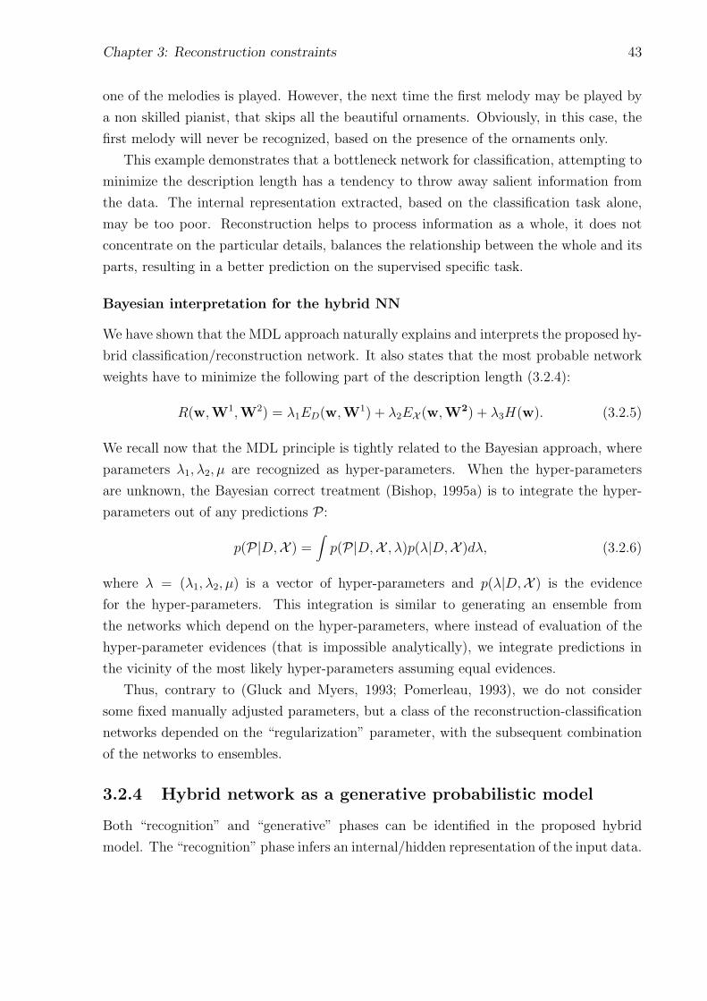
Chapter 3: Reconstruction constraints 43
one of the melodies is played. However, the next time the first melody may be played by
a non skilled pianist, that skips all the beautiful ornaments. Obviously, in this case, the
first melody will never be recognized, based on the presence of the ornaments only.
This example demonstrates that a bottleneck network for classification, attempting to
minimize the description length has a tendency to throw away salient information from
the data. The internal representation extracted, based on the classification task alone,
may be too poor. Reconstruction helps to process information as a whole, it does not
concentrate on the particular details, balances the relationship between the whole and its
parts, resulting in a better prediction on the supervised specific task.
Bayesian interpretation for the hybrid NN
We have shown that the MDL approach naturally explains and interprets the proposed hy-
brid classification/reconstruction network. It also states that the most probable network
weights have to minimize the following part of the description length (3.2.4):
R(w,W1,W2) = λ1ED(w,W1) + λ2EX (w,W2) + λ3H(w). (3.2.5)
We recall now that the MDL principle is tightly related to the Bayesian approach, where
parameters λ1, λ2, µ are recognized as hyper-parameters. When the hyper-parameters
are unknown, the Bayesian correct treatment (Bishop, 1995a) is to integrate the hyper-
parameters out of any predictions P :
p(P|D,X ) =∫p(P|D,X , λ)p(λ|D,X )dλ, (3.2.6)
where λ = (λ1, λ2, µ) is a vector of hyper-parameters and p(λ|D,X ) is the evidence
for the hyper-parameters. This integration is similar to generating an ensemble from
the networks which depend on the hyper-parameters, where instead of evaluation of the
hyper-parameter evidences (that is impossible analytically), we integrate predictions in
the vicinity of the most likely hyper-parameters assuming equal evidences.
Thus, contrary to (Gluck and Myers, 1993; Pomerleau, 1993), we do not consider
some fixed manually adjusted parameters, but a class of the reconstruction-classification
networks depended on the “regularization” parameter, with the subsequent combination
of the networks to ensembles.
3.2.4 Hybrid network as a generative probabilistic model
Both “recognition” and “generative” phases can be identified in the proposed hybrid
model. The “recognition” phase infers an internal/hidden representation of the input data.

Chapter 3: Reconstruction constraints 44
The “generative” phase reconstructs the input from the inferred compact representation
in the reconstruction output sublayer and, in addition, predicts the specific task output
in the corresponding sublayer.
From a Bayesian viewpoint, learning in the hybrid network is equivalent to maximiza-
tion of the joint probability of the input and specific task output, given the observation
and specific constraints on the internal representation. According to Bayesian theory, the
best classification is based on the conditional probability of the image classes given the
input (i.e. the conditional probabilities of the image classes are the best discriminant
functions, that lead to the minimal classification error). The output of the recognition
layer of the hybrid network estimates this conditional probability and the reconstruction
sublayer regenerates the input data, implicitly estimating the probability of the input
data.
The proposed architecture differs from a probability network that has a generative
model (reconstruction) and a recognition model in a manner similar to the binary wake/sleep
architecture (Hinton et al., 1995), or the Rectified Gaussian Belief Network (Hinton and
Ghahramani, 1997). First, it is not a full forward/backward model, namely there are no
two hidden unit representations, one for the top-down and one for the bottom-up, but
instead a single hidden representation is used for both (Figure 3.3). Second, its learning
goal is to minimize the classification error (via the mean squared error) as well as to
minimize the reconstruction error, as opposed to the goal of constructing a probabilistic
model of internal representations. The two goals may coincide under a continuous hidden
unit network, but are certainly different for a binary network.
3.2.5 Hybrid Neural Network architecture
The detailed architecture of the network is presented in Figure 3.5. This hybrid network
is a modification of the well-known feed-forward network. It is supplied by images in the
input layer which are propagated via a hidden layer to the output layer. The output layer
consists of two sub-layers, one sub-layer reconstructs the image, the second one serves
for classification. The number of units in the output reconstruction sub-layer and the
input layer are the number of pixels in the image. The hidden layer has a smaller number
of units, because we are looking for aggressive compression techniques to overcome the
“curse of dimensionality”. The output classification layer has a number of units equal to
the number of image classes. Each image is propagated to the hidden layer in the form:
hj =N∑
i=1
wjixi + wj0 (3.2.7)
yj = σ(hj), j = 1, . . . ,m, (3.2.8)
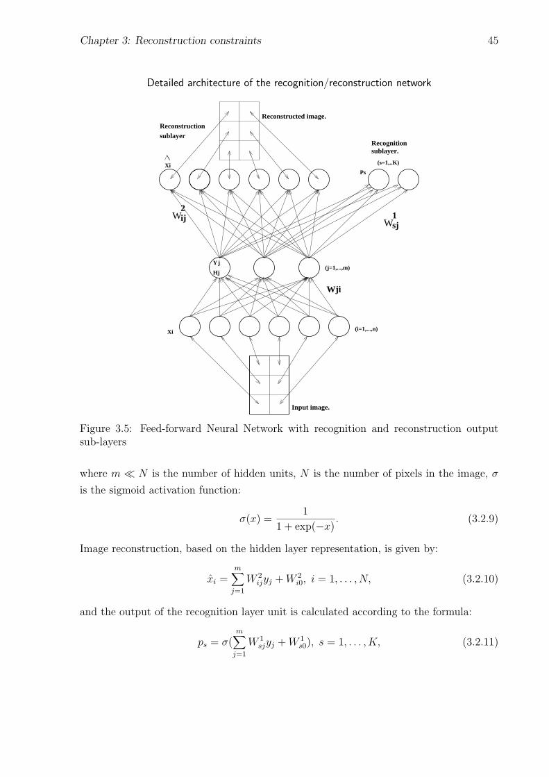
Chapter 3: Reconstruction constraints 45
Detailed architecture of the recognition/reconstruction network
sublayerReconstruction
(s=1,..K)
PsXi
j
Reconstructed image.
sj1
W
Input image.
sublayer.Recognition
Y
Hj(j=1,...,m)
(i=1,...,n)
Wji
Xi
ij2
W
Figure 3.5: Feed-forward Neural Network with recognition and reconstruction outputsub-layers
where m N is the number of hidden units, N is the number of pixels in the image, σ
is the sigmoid activation function:
σ(x) =1
1 + exp(−x). (3.2.9)
Image reconstruction, based on the hidden layer representation, is given by:
xi =m∑
j=1
W 2ijyj +W 2
i0, i = 1, . . . , N, (3.2.10)
and the output of the recognition layer unit is calculated according to the formula:
ps = σ(m∑
j=1
W 1sjyj +W 1
s0), s = 1, . . . , K, (3.2.11)

Chapter 3: Reconstruction constraints 46
where K is the number of individuals (number of classes). The classification is made
according to the maximal response of the recognition sub-layer (ps is interpreted as the
probability of the sample to belong to a certain class -s).
3.2.6 Network learning rule
Let us consider the error back-propagation learning rule with a goal of minimizing the
cost function, which is a weighted sum of scaled recognition and reconstruction errors
with coefficients λ1 and λ2, respectively1:
E(w,W1,W2) = λ1E1(w,W1)/K + λ2E
2(w,W2)/N. (3.2.12)
As has been shown in the Section 3.2.3, the coefficients λ1 and λ2 are inversely propor-
tional to the noise variances in the reconstruction and recognition channels, respectively.
Therefore, the larger the noise is in the channel, the less is the weight of the error-cost
corresponding to this channel. Recognition E1 and reconstruction E2 errors, sum squared
over all samples are given by:
E1 =M∑
µ=1
K∑
s=1
(pµs − tµs )2. (3.2.13)
E2 =M∑
µ=1
N∑
i=1
(xµi − t(xµi ))2 (3.2.14)
In this expression, t(xµi ) determines the target of the µ-sample in the reconstruction
unit-i. The most reasonable choice for t(xµi ), not demanding any a-priory knowledge, is
t(xµi ) = xµi . Correspondingly, tµs is a target for recognition given by:
tµs =
1 if s coincides with class of µ-sample0 otherwise
The weights between output-to-hidden and hidden-to-input layers update according
to the gradient descent rule :
∆W1 = −η?λ15W1 E1(w,W1) (3.2.15)
∆W2 = −η?λ25W2 E2(w,W2) (3.2.16)
∆w = −η?(λ15w E1 + λ25w E2) (3.2.17)
1For convenience, scaling of errors E1 and E2 by the number of pixels in the image N , and the numberof image classes K respectively is carried on. This scaling serves to balance the values of the recognitionand reconstruction errors in Eq. 3.2.4.
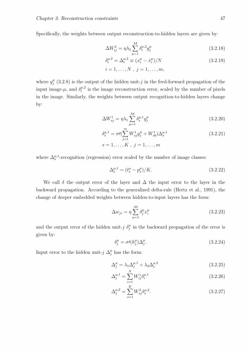
Chapter 3: Reconstruction constraints 47
Specifically, the weights between output reconstruction-to-hidden layers are given by:
∆W 2ij = ηλ2
M∑
µ=1
δµ,2i yµj (3.2.18)
δµ,2i = ∆µ,2i ≡ (xµi − xµi )/N (3.2.19)
i = 1, . . . , N , j = 1, . . . ,m,
where yµj (3.2.8) is the output of the hidden unit-j in the feed-forward propagation of the
input image-µ, and δµ,2i is the image reconstruction error, scaled by the number of pixels
in the image. Similarly, the weights between output recognition-to-hidden layers change
by:
∆W 1sj = ηλ1
M∑
µ=1
δµ,1s yµj (3.2.20)
δµ,1s = σ′(m∑
j=1
W 1sjy
µj +W 1
s0)∆µ,1s (3.2.21)
s = 1, . . . , K , j = 1, . . . ,m
where ∆µ,1s -recognition (regression) error scaled by the number of image classes:
∆µ,1s = (tµs − pµs )/K. (3.2.22)
We call δ the output error of the layer and ∆ the input error to the layer in the
backward propagation. According to the generalized delta-rule (Hertz et al., 1991), the
change of deeper embedded weights between hidden-to-input layers has the form:
∆wji = ηM∑
µ=1
δµj xµi (3.2.23)
and the output error of the hidden unit-j δµj in the backward propagation of the error is
given by:
δµj = σ′(hµj )∆µj . (3.2.24)
Input error to the hidden unit-j ∆µj has the form:
∆µj = λ1∆µ,1
j + λ2∆µ,2j (3.2.25)
∆µ,1j =
N∑
i=1
W 1ijδ
µ,1i (3.2.26)
∆µ,2j =
K∑
s=1
W 2sjδ
µ,2s . (3.2.27)

Chapter 3: Reconstruction constraints 48
From (3.2.25–3.2.27) it is easy to see that the output error δµj may be written as the
sum of the errors back propagated concurrently from the reconstruction and recognition
sub-layers:
δµj = λ1δµ,1j + λ2δ
µ,2j (3.2.28)
δµ,1j = σ′(hµj )∆µ,1j (3.2.29)
δµ,2j = σ′(hµj )∆µ,2j . (3.2.30)
In general, the input/output errors to any layer of the network are a weighted sum
of the input/output errors back propagated from the lateral sub-layers (a chain rule of
the derivatives). Thus, in the error back-propagation mode, hybrid network with lateral
sub-layers emerges as a linear superposition of the conventional (classical) subnetworks.
3.2.7 Hybrid learning rule.
We follow the gradient descent algorithm as the errors are back propagated from an input
layer to a hidden layer with a properly scaled cost function (3.2.12):
E(w,W1,W2) = (1− λ)E1(w,W1)/K + λE2(w,W2)/N, (3.2.31)
where λ ∈ [0, 1] (λ = λ2/(λ1 + λ2)) is a regularization parameter, which represents a
tradeoff between reconstruction and classification confidences.
According to the gradient descent method, updating of the weight vector in each
iteration has to be done in the direction that has a negative projection on the gradient
direction. This permits us to rescale a learning rule (3.2.15-3.2.16):
∆W1 = −η?5W1 E1(w,W1)
∆W2 = −η?5W2 E2(w,W2)
∆w = −η?((1− λ)5w E1 + λ5w E2) (3.2.32)
We emphasize that the parameter λ in our implementation, affects only the weights w
between input and hidden layers, i.e. on the hidden layer representation. Our rule (3.2.32)
may be treated as the hidden layer belief in the performance of the two upper channels,
transferring backward information from reconstruction and recognition sub-layers. Thus,
we take the errors of the reconstruction layer with the weight λ, and the errors of the
recognition layer with the weight 1 − λ. It can be seen, that for λ = 0 the hidden
representation is built based only on the recognition task, and reconstruction is learned
from the hidden layer. This marginal case corresponds to the Baluja consideration (Baluja
and Pomerleau, 1995). In contrast, when λ = 1, the hidden representation is based on the
Chapter 3: Reconstruction constraints 49
reconstruction task solely; and we attempt to solve the recognition task in the reduced
space. We see that this marginal case is equivalent to a first approach to classify via
reconstruction (Kirby and Sirovich, 1990; Turk and Pentland, 1991; Murase and Nayar,
1993).
This network and its hybrid rule may be interpreted as the parallel concurrent work
of two separate feed-forward networks for recognition and reconstruction. The hybrid net
hidden weight updating is a linear combination of the gradient directions of both networks
in the common hidden weight space. For small λ our method is a kind of gradient descent
method that prevents zig-zags (peculiar to the gradient steepest descent method (Ripley,
1996)) in the search of the optimal weights minimizing the recognition regression error.
Chapter 4
Imposing bias via unsupervisedlearning constraints
4.1 Introduction
Information theory provides some explanation to sensory processing (Rieke et al., 1996).
According to these principles, neural cell responses are developed by optimizing criterions
based on the information theory. The first proposed information principles are redundancy
reduction (Barlow, 1961) and “infomax” (Linsker, 1988), that are similar and lead to a
factorial code formation under some conditions (Nadal and Parga, 1994). Recently, with
the parallel development of independent component analysis (ICA) (Comon, 1994) in
the signal processing, new efficient algorithms for the factorial code formation have been
proposed. Of particular interest are algorithms via feed-forward networks with no hidden
layer (Bell and Sejnowski, 1995; Yang and Amari, 1997).
In this chapter, we propose to use information theoretical measures as constraints for
the classification task. We introduce a hybrid neural network with a hidden representa-
tion that is arranged mainly for the classification task and, in addition, has some useful
properties, such as the independence of hidden neurons or maximum information transfer
in the hidden layer, etc.
The chapter is organized as follows. In the first section, the main information principles
and their relation to sensory processing are discussed. The second section presents the
mathematical background and algorithms for ICA and other related information prin-
ciples. In the third section, a hybrid neural network with unsupervised constraints is
introduced and some algorithmical details are presented.
50

Chapter 4: Unsupervised learning constraints 51
4.2 Information principles for sensory processing
Mammals process incomplete and noisy sensory information in an apparently effortless
way. This is possible since sensory inputs: images, sounds, etc., have very specific
statistical properties that are efficiently encoded by the biological nervous systems. The
sensory inputs appear usually smooth over large spatial and temporal regions that lead
to redundancy in the sensory input. The redundancy emerges as a statistical regularity,
which means that many pieces of a signal are a-priori predictable from other pieces and
hence by clever recoding it is possible to get more economical representation of the data.
In the past, the principle of redundancy reduction (Barlow, 1961) was suggested as a
coding strategy in neurons. According to this principle each neuron should encode features
that are as statistically independent as possible from other neurons over a natural ensemble
of inputs. The ultimate obtained representation is called the factorial code (Redlich, 1993).
In the factorial code, the multivariate probability density function (pdf) is factorized as
a product of marginal pdfs. This property provides an efficient way of storing statistical
knowledge 1 about the input (Barlow, 1989).
One of the earliest attempts to construct the factorial representation via neural net-
works was proposed by Atick (1992). The underlying computational learning rule is based
on the minimization of the sum of the entropies of the hidden units under constraint to
preserve the input entropy (the total information about the signal). A type of gradient
descent algorithm in the assumption of a Gaussian input signal and linear output, re-
sults in a Hebbian-like learning rule and a decorrelated hidden representation. The major
limitation of Hebbian-like rules is dependence on the linear, pairwise correlations among
image pixels (second order statistics). Thus, they are not sensitive to phase changes in
the image responsible for oriented localized structures, such as lines, edges and corners
(Field, 1994).
Motivated by the principle of redundancy reduction Field (1994) contrasts two different
coding approaches. Both approaches take advantage of the input redundancy, but in a
different manner. The first one, compact coding, is based on the mean-squared error and
uses only the second order statistics of the input. The main goal of this coding is to
reduce dimensionality of the input in the directions with a low input variance. PCA
and linear auto-associator networks, considered in Chapter 3, are examples of this coding
scheme. An alternative sparse distributed coding does not necessarily imply the reduction
of dimensionality. In contrast, the dimensionality may be enlarged. A sparse distributed
1For an image description the probability of each possible set of pixel values has to be known. Forinstance, an image having N pixels with Q intensity quantization levels requires the storing of QN possibleprobabilities. If the code is factorial the number of the required probabilities reduces to NQ.

Chapter 4: Unsupervised learning constraints 52
coding approach encourages representations, where only a small, adaptive to input, subset
of hidden units is simultaneously active.
Although, there is not a general tool to form the sparse code, it has some typical
features. The sparse code is characterized by the extremely peaked distribution of the
hidden unit activities which provides both high probability of a neuron to be silent or
active according to its relevance to the input pattern representation. A way to construct
sparse coding based on this feature has been proposed in (Olshausen and Field, 1996) by
minimizing the cost functional consisting of a mean-squared error and a penalty term for
neuron activities.
Peaked distributions are characterized by high kurtosis or low entropies (Oja, 1995b),
thus, maximization of kurtosis or entropy minimization can be used for sparse coding
formation. At the same time, via minimization of the sum of the entropies sparse coding
is related to a factorial coding. It is also known that under a fixed variance the Gaussian
distribution has the largest entropy (Cover and Thomas, 1991). Thus, hidden unit entropy
minimization is tightly related to exploratory projection pursuit (EPP), which tries to
find a structure in the projected data, seeking directions that are as far from Gaussian as
possible (Friedman, 1987). Therefore, a deviation from the Gaussian distribution serves
as a good measure for hidden unit independence and can be used as a strategy for sparse
coding construction.
Recently, an interest in EPP has been revived and formulation of the new unsuper-
vised rules based on the information theory has been stimulated with the development of
independent component analysis (ICA). In the next section, ICA is formulated and some
algorithms producing factorial codes are presented.
4.3 Mathematical background
ICA has been developed as a tool for blind source separation. The problem is to recover
independent sources from sensory observations which are unknown linear mixtures of the
unobserved independent source signals. Let us consider m unknown mutually independent
sources si(t), i = 1, . . . ,m with no more than one being normally distributed. In general,
t is a sampling variable, that may be a time variable for signals or a two dimensional
spatial variable for images, or an index of the pattern in a data-set. The sources are
mixed together linearly by an unknown non-singular matrix A ∈ Rn×m:
x(t) = As(t), s(t) = [s1(t), . . . , sm(t)] (4.3.1)
It is assumed that in (4.3.1) the number of sensors xi(t), i = 1, . . . n is greater or equal
to the number of sources (n ≥ m). The task is to recover the original signals via a linear

Chapter 4: Unsupervised learning constraints 53
transform defined by a matrix W ∈ Rm×n:
u(t) = Wx(t), u(t) = [u1(t), . . . , um(t)] (4.3.2)
Since recovered signals may be permuted and scaled versions of the sources, the de-mixing
matrix W has to be a solution of the following linear equation:
ΛP = WA,
where Λ is a non-singular diagonal matrix and P is a permutation matrix.
4.3.1 Entropy maximization (ME)
One of the first algorithms extracting the independent components via a neural network
has been proposed by Bell et al. (1995). Assuming that the number of sources is equal
to the number of sensors, a fully connected n → n feed-forward network consisting from
an input and nonlinear output layers, having the same number of units as the number of
sources, has been considered (Figure 4.1). The network has been trained to maximize a
Feed-forward network for independent component extraction
y i =g i (u i )
uiy i
u=Wx
Input - x
(u-recovered sources)
Output y:
Figure 4.1: A one layer n→ n feed-forward network.
joint entropy H(y) of the nonlinear output y:
u = Wx + w0, y = g(u), y ∈ Rn,u ∈ Rn,w0 ∈ Rn (4.3.3)
H(y) = −∫p(y) log p(y)dy
In the case of the output additive noise, the entropy maximization (ME) is equivalent
to maximization of the mutual information between input and output (Nadal and Parga,

Chapter 4: Unsupervised learning constraints 54
1994). As has been shown earlier (Linsker, 1988), the principle of the mutual informa-
tion maximization called “infomax” in the case of a linear neural network leads to a
Hebbian like learning rule, that is sensitive to the second order statistics only, therefore,
nonlinearity in the output layer is essential.
The joint entropy of the output can be represented as:
H(y) =∑
i
H(yi)− I(y), (4.3.4)
where H(yi) = − ∫ p(yi) log p(yi)dyi are marginal entropies of the outputs and I(y) is
their mutual information. The mutual information (MI) of the output y is a Kullback-
Leibler measure between output distribution p(y) and a product of marginal distributions∏i p(yi):
I(y) =∫p(y) log
p(y)∏i p(yi)
dy (4.3.5)
Due to a ∩-convexity of the log function, the Kullback-Leibler measure is nonnegative and
attains its minimum zero value if and only if outputs yi are independent almost every-
where. Maximization of the joint entropy consists of maximizing the marginal entropies
and minimizing the mutual information. Since the nonlinear functions bound the outputs,
the marginal entropies are maximum for a uniform distribution of yi. The mutual infor-
mation I(y) is invariant under an invertible component-wise transform (I(y) = I(u)) and
achieves its minimum equal zero when the presynaptic outputs u (4.3.3) are independent.
Thus, if the nonlinear functions gi have the form of the cumulative density function (cdfs)
of the true source distribution, then the matrix W recovers independent sources as the
presynaptic output u (4.3.3), and this is a single global maximum of the joint entropy
H(y), which is a convex ∩ function.
As has been rigorously proven (Yang and Amari, 1997), the ME approach leads to
the independent components only if the nonlinear activation functions gi in the output
layer coincide with the cumulative density functions (cdfs) of the sources. For zero mean
mixtures and functions gi not equal to the (cdfs) of the sources, the ME algorithm does
not converge to the ICA solution W = ΛPA−1. However, if the initial matrix is the right
ICA solution W0 = ΛPA−1
, the algorithm does not update the de-mixing matrix W in
the directions of increasing the cross-talking. This fact partially explains the ME success,
even when cdfs are not known exactly. In applications considered by Bell and Sejnowski
(1995), nonlinear activation functions have been chosen ad hoc as logistic sigmoidal, that
has a highly peaked derivative with long tails. Since sound signals are super-Gaussians2
this type of nonlinearity appears to be appropriate for “infomax” principle.
2Super-Gaussian signals have pdf with large tail areas and a sharp peak. In contrast, sub-Gaussiansignals have pdf with small tail areas and a flat peak (see also Appendix A to Chapter 4.)

Chapter 4: Unsupervised learning constraints 55
The de-mixing matrix W is found as synaptic weights of the network iteratively using
the stochastic gradient ascent method applied to the joint entropy H(y):
∆W = η([Wt]−1 + (1− 2y)xt) 1 ∈ Rn,
∆w0 = η(1− 2y)
Amari et al. (1997) have suggested a modification of this rule that utilizes the nat-
ural gradient and does not require the inversion of the weight matrix. It proceeds by
multiplying the absolute gradient by WtW, producing3:
∆W = η(I + (1− 2y)ut)W (4.3.6)
4.3.2 Minimization of the output mutual information (MMI)
Another way to derive independent outputs for the blind separation problem has been
presented in (Amari et al., 1996). An algorithm minimizes the mutual information (MI)
of the linear outputs, Iu(W):
Iu(W) = −H(u) +n∑
i=1
H(ui), (4.3.7)
u = Wx, (4.3.8)
that attains its minimum if and only if the outputs ui are independent about everywhere.
In order to approximate marginal entropies H(ui), truncated Gram-Charlier expansion
(Stuart and Ord, 1994) of the marginal pdfs p(ui) has been used and a mild assumption
about the original source statistics has been done. It has been assumed that the original
sources have zero mean and their variances are normalized to 1. A stochastic gradient
descent applied to the approximated expression of the mutual information Iu(W) leads
to the following equation for the network weight dynamics:
∆W = η([Wt]−1 −Φ(u)xt) (4.3.9)
where Φ(u) = f(k3,k4) u2 + g(k3,k4) u3 and the following notations have a place:
f y = [f1y1, . . . , fnyn]t, uk = u uk−1
f(k3,k4) = [f(k13, k
14), . . . , f(kn3 , k
n4 )]t, g(k3,k4) = [g(k1
3, k14), . . . , g(kn3 , k
n4 )]t
ki3 = mi3 = E[u3
i ], ki4 = E[u4i ]− 3(E[u2
i ])2
f(a, b) = −1
2a+
9
4ab, g(a, b) = −1
6b+
3
2a2 +
3
4b2
3w0 is assumed to be zero.

Chapter 4: Unsupervised learning constraints 56
The natural gradient descent for MMI leads to the following algorithm:
∆W = η(t)[I−Φ(u)ut]W (4.3.10)
As has been pointed out in (Yang and Amari, 1997), both ME and MMI algorithms
have the same typical form (4.3.10). In ME Φ depends on the nonlinear activation
functions gi and is given by:
Φ(u) = −(g′′1(u1)
g′1(u1), . . . ,
g′′n(un)
g′n(un))t (4.3.11)
Since gi should coincide with the cdfs of the unknown original signals, Φ(u) have to
be chosen properly. In MMI, functions Φ depend on the cumulants of the third and
fourth orders ki3, ki4 of the linear scalar output ui. These cumulants may be replaced by
instantaneous values or be estimated. Another possibility is to use a-priori knowledge
about cumulants of the unknown original signals. Therefore, whereas a success of the
ME algorithm depends on the a-priori knowledge about data statistics, MMI is more
flexible.
In (Yang and Amari, 1997) the following types of Φ(u) = (φ(u1), . . . , φ(un))t have
been used:
(a) φ(u) = u3 (4.3.12)
(b) φ(u) = tanh(u) (4.3.13)
(c) φ(u) =3
4u11 +
15
4u9 − 14
3u7 − 29
4u5 +
29
4u3 (4.3.14)
The (a-b) forms of Φ(u) correspond to the ME algorithm and assume pdfs (and equiva-
lently g(u)) 4 to be proportional to:
(a) p(u) ∝ exp(−u4/4) (4.3.15)
(b) p(u) ∝ (cosh(u))−1 (4.3.16)
Therefore in both cases, distributions are assumed to be symmetrical and sub-Gaussian.
The form (4.3.14) of Φ(u) is the instantaneous form of MMI (ki3 = u3i , k
i4 = u3
i − 3) and
it does not assume the shape of the source distributions.
The ME and MMI learning rule (4.3.10) has been obtained in the assumption of a
square weight matrix, W. However, in some applications it may be interesting to separate
4Here we use the fact that − g′′(u)g′(u) = φ(u), which leads to g′(u) = exp(− ∫ u
0φ(u))du and at the same
time g′(u) must coincide with pdfs of the original sources.

Chapter 4: Unsupervised learning constraints 57
only a part of the sources. This may be done via multiplication of the right side of the
learning rule (4.3.9) by WtΛW, where the block matrix Λ ∈ Rn×n is given by :
Λ =
(I 00t 0s
). (4.3.17)
In (4.3.17) I ∈ Rm×m is an identity square matrix, 0 ∈ Rm×(n−m) is a rectangular zero
matrix, 0s ∈ R(n−m)×(n−m) is a square zero matrix and m < n. The final learning rule for
a part of the weight matrix W, obtained by deleting the last (n−m) rows of the matrix
W will be the same one as (4.3.10): W ∈ Rm×n:
∆W = η(t)[I−Φ(u)ut]W
W ∈ Rm×n, Φ(u) ∈ Rm×1, u ∈ Rm×1, I ∈ Rm×m
The network architecture then implies dimensionality reduction since the number of out-
put units is less than the number of input units. In addition, such a network extracts
independent components.
4.3.3 Relation to Exploratory Projection Pursuit.
MMI has been considered as the starting point for a large family of ICA contrast functions
proposed by Hyvarinen (Hyvarinen, 1997a). It has been noted that MI can be expressed
using negentropies J(u), J(ui)5 (Hyvarinen, 1997a; Girolami and Fyfe, 1996):
Iu(W) = J(u)−∑i
J(ui) +1
2log
∏iCii
det(C), (4.3.18)
where C is a covariance matrix of u and Cii are its diagonal elements. Since the negentropy
J(u) is invariant for invertible linear transformations (J(u) = J(x), note that J(ui) =
J(xi) holds only when nonlinear transformation: x → u, is componentwise with ui =
f(xi)), MMI is roughly equivalent to finding directions in which negentropy is maximized.
This equivalence is rigorous, when components ui are constrained to be uncorrelated (the
last term of 4.3.18 is zero). This means that the directions in which the data distribution
is as non-Gaussian as possible are preferable. This is the point where EPP and ICA have
come into contact.
The natural gradient ascent applied to the sum of the marginal negentropies leads to
the same learning rule (4.3.10) (Girolami and Fyfe, 1996; Lee et al., 1998). When the
5Negentropy of the multivariate random variable u is a difference between entropies of the multivariateGaussian distribution with the same covariance matrix as u and entropy of the u: J(u) = H(uG)−H(u).It measures deviation of the distribution from Gaussian and is nonnegative. The valuable property ofnegentropy is invariance under invertible linear transforms.

Chapter 4: Unsupervised learning constraints 58
nonlinearities Φ are taken to be:
φi(ui) =
ui + tanh(ui) for super-Gaussian sourceui − tanh(ui) for sub-Gaussian source
the learning rule may be written in the elegant form:
∆W = η(t)[I−K tanh(u)ut − uut]W, (4.3.19)
where K is a diagonal matrix with elements sign(kur(ui)) and kur(ui) is kurtosis of the
i-source.
The advantage of EPP, however, is the possibility to find independent components
recursively one-by-one by maximization of the 1-D negentropy. For the same conditions,
as in (Yang and Amari, 1997): E[ui] = 0, E[u2i ] = 1, negentropy may be approximated
by:
J(ui) ≈ 1
12(E(u3
i ))2 +
1
48(k4(ui))
2 (4.3.20)
When source distributions are assumed to be symmetrical, negentropy simplifies to J(ui) ∝(k4(ui))
2 = kur2i and minimization of the output mutual information is approximately
equivalent to maximization of the sum of the source kurtosises6:
Fmax(W) =∑
kur2i (4.3.21)
In other words, the directions in which signal distribution is highly peaked or extremely
flat, are considered as interesting.
In (Hyvarinen, 1997b) a new family of approximated contrast ICA functions has been
proposed via the negentropy approximation:
J(u) ∝ (E[G(u)]− E[G(ν)])2, (4.3.22)
where ν is a standardized Gaussian variable and the function G fulfills some orthogonality
property and is suitable to the assumed original source statistics and is reasonably simple
for computation. The simplest proposed choices for the function G is polynomial G = |u|α,
where α < 2 for super-Gaussian densities and α > 2 for sub-Gaussian densities. This
approach appears finally as a generalization of different projection pursuit indices (Blais
et al., 1998), where skewness and kurtosis are used explicitly to measure deviation from
the Gaussian distribution. It is related also to the BCM neuron learning rule (Intrator
and Cooper, 1992).
6See Appendix A to Chapter 4 for cumulants and kurtosises definitions.

Chapter 4: Unsupervised learning constraints 59
4.3.4 BCM
An idea of BCM is to find a direction w which emphasizes data multi-modality by mini-
mizing a specific loss function (a specific projection index):
F(w) = −µ(1
3E[u3]− 1
4θ2) (4.3.23)
u = wtx, θ = E[u2],
In order to make this measure robust to outliers, a rectification nonlinear function is
applied in the linear output. Thus, in general, y = g(wtx). The gradient descent rule
yields the following learning rule:
∆w = µE[φ(y, θ)g′(u)x] (4.3.24)
where φ(y, θ) = y2 − yθ, θ = E[y2].
4.3.5 Sum of entropies of the hidden units
Being motivated to obtain a hidden representation where each neuron contains as much
information as possible, we suggest to maximize the sum of the entropies of the output
units:
F(W) =m∑
i=1
H(yi).
The stochastic gradient descent method leads to the following equation for the weight
dynamics (details are given in Appendix B to Chapter 4:
∆W = η(f(u) + g′′g′ )x
t , (4.3.25)
where f(u) is defined as φ(u) in (4.3.14). Since the nonlinear output functions bound the
output values yi, the entropy is maximized, when yi is uniformly distributed, which leads
to a relation pu(ui) = dgidui
. This means that the distribution of the presynaptic variables
ui is controlled by the nonlinearities in the learning rule (4.3.25).
For logistic sigmoidal activation functions, (4.3.25) simplifies to:
∆W = η(f(u) + (1− 2y))xt (4.3.26)
The same rule, but with the negative parameter η, can be used for a sparse code formation,
as suggested in (Olshausen and Field, 1996; Atick, 1992)7.
7When the output is bounded c < y < d, due to a ∩-convexity of the log function, the entropy of theoutput is upper bounded: H(y) =
∫ dcp(y) log 1
p(y)dy ≤ log(∫ p(y)p(y) )dy = log(d− c). Therefore, the entropy
maximization is properly defined mathematically. At the same time the lower estimate depends on thedistribution: −H(y) =
∫ dcp(y) log p(y)dy ≤ log
∫ dc
(p(y))2dy ≤ 2 log((d − c) max p(y)). It is clear thatin practice max p(y) is bounded and therefore, the problem of the sum of entropies minimization is alsoproperly defined mathematically.

Chapter 4: Unsupervised learning constraints 60
4.3.6 Nonlinear PCA
Although the nonlinear PCA method has no apparent connection to the ME or MMI,
it has been shown that it allows separation of the whitened linear mixtures of sources
(Oja, 1995b; Oja, 1995a). In nonlinear PCA, the input signals are first prewhitened, i.e.
the signals are represented as the projections on the eigenspace of the input covariance
matrix and are properly scaled. As a result prewhitened signal x has a zero mean and a
unit spherical covariance matrix. The learning rule is an approximate stochastic gradient
descent algorithm that minimizes the mean-squared reconstruction error:
E = E[‖ x−Wty ‖2], (4.3.27)
where the weight matrix W and nonlinear output y are defined to be the same as in
(4.3.3) and the bias is assumed to be zero w0 = 0.
An approximate learning rule has the form:
∆W = ηy(xt − ytW) (4.3.28)
For separation, odd twice differentiable nonlinear functions gi have to be properly taken
to satisfy some stability conditions depending on the data statistics. Particularly, it is
shown (Oja, 1995a) that a sigmoidal nonlinear activation function as g = tanh(βu), β > 0
is feasible for sub-Gaussian original signals and polynomial g = u3 for super-Gaussian
densities (in this analysis it was assumed that the sources are statistically identical and
have a symmetrical distribution).
The MSE for whitened data and nonlinear activation functions in the form g(u) = u3
or tanh(u) may be approximated as −∑ kuri (Lee et al., 1998). Thus, minimization of
the MSE leads to maximization of the sum of the kurtosises:
Fmax(W) =∑
kuri (4.3.29)
The latter expression is equivalent to (4.3.21) for super-Gaussian original sources. This
evaluation shows that in some cases the nonlinear PCA can also be viewed from information-
theoretic principals, as a method to minimize approximately the mutual information of
the output.
4.3.7 Reconstruction issue
Learning in the nonlinear PCA and nonlinear autoencoders is based on the reconstruction
mean-squared error. Similarly to a linear case, nonlinear PCA and nonlinear autoencoder
extract different weights. The nonlinear autoencoder with proper activation functions does

Chapter 4: Unsupervised learning constraints 61
not necessary extract the independent components as the nonlinear PCA does in some
cases. However, this consideration sheds light on the relation between the unsupervised
learning based on the information theory and reconstruction.
Reconstruction and ICA are related also via a generative model approach (MacKay,
1996; Roweis and Ghahramani, 1997; Lee et al., 1998). ICA recovering independent com-
ponents (hidden variables) and de-mixing weight matrix W is itself a recognition phase
of the reconstruction process, with a nonlinear generative model that differs from genera-
tive models underlying PCA and linear autoencoder. Thus, although ICA (information-
theoretic) constraints may be also considered as some type of “generalized” reconstruction
constraints with another underlying generative model, we keep the notion of reconstruc-
tion constraints for an autoencoder network.
ICA similar to PCA has been also used as a preprocessing step for face classification
(Bartlett et al., 1998). As will be clear later, the hybrid classification/feature extraction
scheme which is introduced in the next section corresponds to this type of preprocessing,
when trade-off parameter λ = 1.
4.4 Imposing unsupervised constraints
The unsupervised learning rules we have used are based on different assumptions about the
quality of the low dimensional representation (LDR). These rules are based on statistics
of order higher than two, and use low order moments of the distribution and a sigmoidal
squashing function for robustness against outliers.
The learning rule for hidden weights modification for the constrained network (Fig-
ure 2.2) is described by:
∆w = −η((1− λ)5w E1 − λh(w,x)), (4.4.30)
where the term h(w,x) corresponds to weight updating, that emerges via additional
unsupervised feature extraction. When h(w,x) is a gradient of some information measure
H(w,x) 8 the learning rule (4.4.30) corresponds to minimization of the penalized mean
squared recognition error:
F(w,W1) = (1− λ)E1(w,W 1)− λH(w,x). (4.4.31)
Table 4.1 summarizes different learning constraints with the corresponding h(w,x)-
function. The bottom rows of Table 4.1 describe a few variations on the sum of entropy
8The term h(w,x) can appear as a gradient of some information measure scaled by a positive definitematrix P(x,w), then in general corresponding H(w,x) may not exist. We use the negative sign beforeh(w,x) term in Eq. 4.4.30 for convenience, since most of the used feature extraction rules are formulatedas a maximization problem.
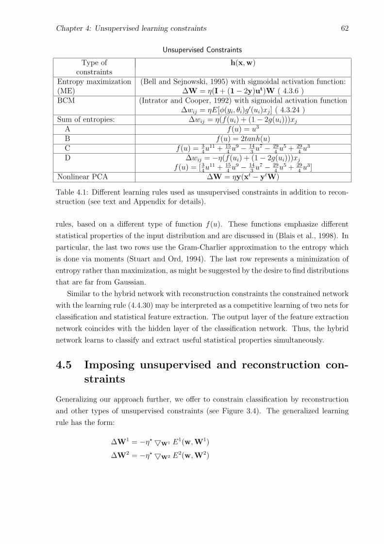
Chapter 4: Unsupervised learning constraints 62
Unsupervised Constraints
Type of h(x,w)constraints
Entropy maximization (Bell and Sejnowski, 1995) with sigmoidal activation function:(ME) ∆W = η(I + (1− 2y)ut)W ( 4.3.6 )BCM (Intrator and Cooper, 1992) with sigmoidal activation function
∆wij = ηE[φ(yi, θi)g′(ui)xj] ( 4.3.24 )
Sum of entropies: ∆wij = η(f(ui) + (1− 2g(ui)))xjA f(u) = u3
B f(u) = 2tanh(u)C f(u) = 3
4u11 + 15
4u9 − 14
3u7 − 29
4u5 + 29
4u3
D ∆wij = −η(f(ui) + (1− 2g(ui)))xjf(u) = [3
4u11 + 15
4u9 − 14
3u7 − 29
4u5 + 29
4u3]
Nonlinear PCA ∆W = ηy(xt − ytW)
Table 4.1: Different learning rules used as unsupervised constraints in addition to recon-struction (see text and Appendix for details).
rules, based on a different type of function f(u). These functions emphasize different
statistical properties of the input distribution and are discussed in (Blais et al., 1998). In
particular, the last two rows use the Gram-Charlier approximation to the entropy which
is done via moments (Stuart and Ord, 1994). The last row represents a minimization of
entropy rather than maximization, as might be suggested by the desire to find distributions
that are far from Gaussian.
Similar to the hybrid network with reconstruction constraints the constrained network
with the learning rule (4.4.30) may be interpreted as a competitive learning of two nets for
classification and statistical feature extraction. The output layer of the feature extraction
network coincides with the hidden layer of the classification network. Thus, the hybrid
network learns to classify and extract useful statistical properties simultaneously.
4.5 Imposing unsupervised and reconstruction con-
straints
Generalizing our approach further, we offer to constrain classification by reconstruction
and other types of unsupervised constraints (see Figure 3.4). The generalized learning
rule has the form:
∆W1 = −η?5W1 E1(w,W1)
∆W2 = −η?5W2 E2(w,W2)

Chapter 4: Unsupervised learning constraints 63
∆w = −η?((1− λ)5w E1 + λ((1− µ)5w E2 − µh(w,x)), (4.5.32)
where now we have two regularization parameters λ and µ. Thus, the most general net-
work corresponds to the goal function (3.2.4) and its flow-chart is presented in Figure 3.4.
Chapter 4: Unsupervised learning constraints 64
Appendix A to Chapter 4: Order statistics
Here we give some definitions and relations between order statistics (see (Stuart and Ord,
1994)).
Definition: Moments of order r about the point a
µ′r =∫ ∞−∞
(x− a)rdF, (4.5.33)
where F is a distribution function.
Definition: Characteristic function c.f.
φ(t) =∫ ∞−∞
exp(itx)dF (4.5.34)
It may be easily seen that moments of distribution µ′r about pont 0 are related to the
r-order derivative drtφ(t) of the characteristic function φ(t) via:
µ′r = (−i)r[drtφ(t)]t=0 (4.5.35)
Another set of statistical measures that are widely used in statistics are cumulants.
Definition: The cumulants are defined by the identity
∞∑
r=1
kr(it)r/r! = log φ(t) (4.5.36)
Thus if a moment of order r µ′r is the coefficient of (it)r/r! in the Taylor series expansion
of the characteristic function φ(t), kr is the coefficient of (it)r/r! in the Taylor series
expansion of log φ(t). Here we present the relation between the first four order statistics:
k1 = µ′1
k2 = µ′2 − µ′21k3 = µ′3 − 3µ′1µ
′2 + 2µ′31
k4 = µ′4 − 4µ′3µ′1 − 3µ′22 + 12µ′2µ
′21 − 6µ′41
In order to describe some interesting properties of the distribution, some other statis-
tical measures have been defined:
Definition: Kurtosis
kur(u) =µ4
µ22
− 3 =k4
k22
(4.5.37)
The kurtosis characterizes the degree of peakedness of the graph of a statistical distri-
bution. It is indicative of the concentration around the mean. Distribution for which
kurtosis is equal to zero is called mesocurtic. Those with positive kurtosis are called

Chapter 4: Unsupervised learning constraints 65
leptokurtic and with negative platycurtic. Kurtosis is equal to zero for Gaussian distri-
bution, is negative for sub-Gaussian and positive for super-Gaussian random variables.
The super-Gaussian random variable is “sharper” than the Gaussian, its pdf has large
tail areas and is more sharply peaked. The pdf of the sub-Gaussian random variable has
smaller tail areas and are also flatter-topped (see Figure 4.2). For a normally distributed
random variable (µ1 = 0 and µ2 = 1), kurtosis coincides with the cumulant of the fourth
order. For a family of the density function:
fα(x) = C1 exp(−C2|x|α), (4.5.38)
where positive constants C1, C2 are the normalization constants that ensure that fα is a
probability density of the unit variance:
C1 = (m2
m31
)1/2; C2 = (m2
m1
)α/2,
where
m1 =∫ ∞−∞
exp(−|x|α)dx =2
αΓ(
1
α) (4.5.39)
m2 =∫ ∞−∞
x2 exp(−|x|α)dx =2
αΓ(
3
α)
The different values of the positive parameter of α exhibit different shapes of the distri-
Pdf’s graphs for a family of the exponential density functions
−10 −8 −6 −4 −2 0 2 4 6 8 100
0.2
0.4
0.6
0.8
1
1.2
1.4
α=0.75
α=2
α=5
Figure 4.2: Sample graphs for a family of the exponential density functions. This figuredemonstrates the typical shapes of the super-Gaussian (α = 0.75), and sub-Gaussian(α = 5) random variables.

Chapter 4: Unsupervised learning constraints 66
bution. The random variable is super-Gaussian for 0.5 < α < 2 and is sub-Gaussian for
α > 2 (Figure 4.2).
Appendix B to Chapter 4: Derivation of the sum of
entropies learning rule
We consider compression of the input x = (x1, x2, . . . , xn) via the following nonlinear
transformation:
ui =n∑
j=1
wijxj + wi0, i = 1, . . . ,m, m < n, yi = g(ui).
u and y are vectors of pre and post-synaptic activations of the hidden layer, wij network
weights and wi0 network biases; and g-is a nonlinear monotone-increasing activation func-
tion. The network architecture is presented in Figure 4.3. As a learning rule we choose
Exploratory projection pursuit network
y i =g i (u i )
uiy i
u=Wx
Output y:
Input - x
Figure 4.3: Feature extraction is achieved via (non linear) projection and dimensionalityreduction
to maximize the sum of the entropies of the hidden units:
F(W) =m∑
i=1
H(yi).
The probability of the output of the hidden unit py(yi) can be written as:
py(yi) =pu(ui)
y′i, where y′i =
dyidui
This leads to: ∫p(yi) ln(p(ui))dyi =
∫p(ui) ln(p(ui))dui,

Chapter 4: Unsupervised learning constraints 67
which implies the following expression for the sum of entropies:
F(W) = E[m∑
i=1
lny′i
p(ui)] = (
m∑
i=1
H(ui))1 + E[(m∑
i=1
ln y′i)2]
Thus, our goal consists of two terms, the first , F1 is the sum of the entropies of the pre-
synaptic activations of the hidden units and was evaluated by Amari et al. (1996) using
the truncated Gram-Charlier expansion to approximate the probability density function
(pdf) pu(ui) and the second, E[F2] represents an expectation of the sum of the log-terms.
The weights W have to be adjusted to maximize F(W). Using a gradient ascent algorithm
we obtain:
∆wij = η(∂F1
∂wij+ E[
∂F2
∂wij])
Replacing the gradient method by a stochastic method we obtain:
∆wij = η(f(ui)xj +∂F2
∂wij),
where f(u) is defined by Amari et al. (1996) and is the same as the function φ(ui) in the
expression (4.3.14). However, in our simulation similar to Amari et al., we use f(u) as in
(4.3.12,4.3.13).
The second term for nonlinearities gi(ui), may be written as:
∂F2
∂W=
g′′
g′xt
g′′
g′= (
g′′1(u1)
g′1(u1), . . . ,
g′′m(um)
g′m(um))t (4.5.40)
Thus, the learning rule simplifies to:
∆W = η(f(u) + g′′g′ )x
t (4.5.41)
The second term for any nonlinear function y = g(u), such that its derivative depends
only on y itself y′u = G(y), can be simplified by the following:
∂ln y′i∂wij
=1
y′i
∂y′i∂wij
=1
y′i
∂y′i∂ui
xj =1
y′iy′i∂G(yi)
∂yixj =
∂G(yi)
∂yixj
For the logistic sigmoidal activation function g(u) = 11+exp (−u)
the derivative G(yi) can be
easily evaluated as G(yi) = y′i = yi(1− yi). Thus, we obtain:
∆wij = η(f(ui) + (1− 2yi))xj. (4.5.42)
Chapter 4: Unsupervised learning constraints 68
The only difference in the ∂F1
∂wijevaluation is the presence of the bias wi0 in (4.5.40).
Therefore, we must require that the expectation of pre-synaptic activations of the hidden
units ui be zero and their second moments be mi2 = E[u2
i ] = 1. This can be achieved
by normalizing u before the calculation of f(ui). Furthermore, the network’s input
is normalized, so that E[x] = 0 and consequently, omitting bias at all (w0 = 0), the
condition E[u] = 0 is automatically satisfied. The second condition mi2 = E[u2
i ] = 1
constrains the norm of W. The same rule, but with the negative η, can be used as a
goal for sparse coding (Olshausen and Field, 1996; Atick, 1992).

Chapter 5
Real world recognition
5.1 Introduction
Real-world object recognition is impeded by natural climate conditions such as fog, rain
or snow and also by other conditions such as partial occlusion and noise. This is fur-
ther complicated by changes in illumination and shadows that are due to movement of
surrounding objects. Some of these factors cause image blur, and all these factors are
crucial for recognition performance and have to be properly addressed during training
and testing.
This chapter addresses face recognition under various image degradations. We com-
pare different regularized recognition networks and different ensembles by testing their
performance on the degraded images. Results on two data-sets under various resolutions
and image degradations are demonstrated. We conclude that a combination that includes
ensembles with reconstruction constraints achieves the best performance on the degraded
images. In addition we show that via saliency maps reconstruction can deemphasize de-
graded regions of the input, thus leading to classification improvement under “Salt and
Pepper” noise.
5.1.1 Face recognition
Face recognition is an active field of research with possible applications in such areas as
man-machine interaction, robotics, access control, automatic search in visual databases
and low bit-rate compression. This task is challenging, since faces do not appear as
fixed image patterns; they can appear anywhere, at any size and orientation and with
varied background (Chellapa et al., 1995). Thus, face detection and normalization are
usually performed that reduce variability caused by these factors. However, such local-
ization preprocessing is not sufficient, since faces are not rigid and lighting conditions
69

Chapter 5: Real world recognition 70
are not uniform. Different facial expressions, changes in hair-style and eyeglasses, and
lighting conditions lead to a large amount of face variability. In some applications, this
normalization may be further complicated by low quality of the images. For example,
systems installed at airports yield foggy, blurred images; cheap cameras, such as those
used for robot navigation, lead to images with low resolution. Thus, face recognition is a
particular case of the training when the variability of the data describing the same class
is comparable with the similarity between different classes (Moses, 1994).
Face recognition approaches can be divided into two basic groups, feature-based meth-
ods (Samal and Iyengar, 1992, survey) and processing images as a whole (Kirby and
Sirovich, 1990; Turk and Pentland, 1991; Moghaddam and Pentland., 1994; Valentin
et al., 1994, survey). Most of the effort in the feature-based methods is focused on finding
individual features (e.g., eyes, mouth, nose, head outline, etc.) and measuring statistical
parameters to describe those features and their relationship. Different methods for feature
extraction were proposed such as template matching (Baron, 1981), deformable templates
(Yuille et al., 1989), combination of perceptual organization and Bayesian networks (Yow
and Cipolla, 1996) and methods using facial symmetry and elementary knowledge of faces
(Reisfeld et al., 1990; Tankus, 1996), etc. However, selecting a set of features that cap-
tures the information required for a face recognition is not easy and there is no a complete
satisfactory solution to it.
An alternative approach, inspired by the Gestalt school of perception (Hochberg, 1974;
Kanizsa and Gaetano, 1970) is to process faces as a whole. One of the method presenting
this approach is PCA, that was used for face recognition (Kirby and Sirovich, 1990; Turk
and Pentland, 1991, see Section 3.1.4 for description). Another way is to process images
via Neural Networks. Under this processing faces are presented as pixel intensity images
and extraction of geometrical relationship, texture and subtle facial details is realized
implicitly. Recognition from intensity images is also sensitive to substantial variations
in lighting conditions, head orientation and size. In order to avoid these problems, an
automatic preprocessing of the faces (i.e., normalization for size and position) is required.
Although this normalization stage is also based on the feature extraction, it is rather
constrained and completed by the definition of eyes and mouth or nose locations.
Among the first network models proposed for face recognition are autoassociative
networks and autoencoders (Valentin et al., 1994, survey). Although these network models
were proposed for recognition, they are trained to reconstruct faces. In autoassociative
networks, the recognition task is constrained to a face familiarity task. The cosine between
every face and its reconstructed version is evaluated and is thresholded to decide if the face
is familiar or not (O’Toole et al., 1991). In the autoencoders, their hidden representation

Chapter 5: Real world recognition 71
has been used as an input for the back-propagation sex and identity networks without
hidden layer (Cotrrell and Fleming, 1990).
Radial basis function (RBF) networks in the context of face recognition have been
first implemented by Edelman et al. (1992). The famous data-set (Turk and Pentland,
1991) described below in Section 5.2.4 has been used in their experiments. The faces
were normalized by the same procedure, as described below in Section 5.2.5, to reduce
variability to viewpoint and illumination direction. A set of Gaussian receptive fields
(RFs) of different size and elongation were applied to reduce dimensionality of the input.
These RFs were applied in different locations inspired by observation RFs of the simple
cells in the primary visual cortex of mammals. Every RBF network was intended for a
certain person recognition and was trained only by positive examples for which a single
output neuron had a desired value equal to 1. The face was considered as recognized
by the individual RBF network if its output exceeded some threshold. Later on, when
training of the individual RBF networks was ended, their outputs were used as inputs to
a new RBF network with the number of output units equal to the number of persons.
The desired activities were taken to be equal to 1 for the neuron responsible for a given
input image, and was equal to 0 for others. The misclassification rate equal to 9% vs.
22% for individual networks was achieved by this new RBF network.
Recently, an interest to RBF networks as a tool for face recognition has been revived.
Different novel variants of the RBF network schemes were proposed (Howell, 1997; Sato
et al., 1998; Gutta et al., 1996). In (Howell, 1997), the hyper RBF network, which has
the number of hidden units equal to the number of training samples and trained on the
images of all persons, is reorganized into a group of smaller face recognition unit networks.
Each face recognition unit network is intended for a particular person recognition and has
two output units. The first unit is responsible for the particular person presence and the
second has to be active when an ”anti” person is presented. The network uses views of the
certain person as positive examples and some selected ambiguous images of other people
as negative ones. Although this approach increases complexity, as more networks need to
be trained, it allows to reduce dimensionality of each unit network and it is adaptive to
a new person addition. When a new person is added, only one additional unit network
has to be trained, and perhaps a small number of ambiguous unit networks needs to be
retrained. A way to combine the standard RBF network with face unit networks based
on their confidences was also proposed.
Ensembles of standard RBF networks for face recognition have been proposed in
(Gutta et al., 1996). Two ensemble variants, defined in terms of their specific topol-
ogy (connections and RBF nodes) and the data they are trained on, were considered.

Chapter 5: Real world recognition 72
In the first variant (ERBF1), three groups of networks, which were trained separately
on the original data, and on the same original data with either some Gaussian noise or
subject to some degree of geometrical distortion were combined. Inside each group three
networks with the different topology were taken. The decision is based on the averaging
of the networks outputs (see Section 2.2) and takes place if the maximal response is larger
than some threshold. In the second variant (ERBF2), three RBF networks with different
topology were trained on the extended data consisting of original data and their corrupted
versions. Later on these ensembles are combined with inductive decision trees classifiers.
Sato et al. (1998) use as input to RBF networks partial face images, such as ears, eyes
and nose, which are cropped by hand. The network is trained with sub-images of known
and unknown images, taken under uniform lighting condition and with the fixed distance
between a camera and subjects. Each output unit of the RBF network corresponds to
the certain person. The input is recognized according to the unit with a maximal output
response, if the latter is larger than some threshold. This threshold is set by hand due
to separability of the maximal responses of known and unknown sub-images. Thus, a
network is also able to reject unknown faces.
A variant of a hybrid supervised/unsupervised network for automatic face recognition
has been proposed by Intrator et al. (1996). A network is trained using a hybrid training
method. This method is based on a formulation that combines unsupervised (exploratory)
methods for finding structure (extracting features) and supervised methods for reducing
classification error. The unsupervised training is based on the biologically motivated BCM
neuron (Intrator and Cooper, 1995) and is aimed at finding hidden units with a multi-
modal distribution of their activities. The supervised portion is aimed at finding features
(in network hidden units) that minimize classification error on the training set. The same
data-set and normalization as in (Edelman et al., 1992) were used. The classification
result for averaged output of five hybrid BCM/recognition was 99.38%, which is better
than using RBF networks (Edelman et al., 1992).
A new approach to face recognition using Support Vector Machines (SVM) has been
proposed by Phillips (1998). SVM is a binary classification method that finds the optimal
linear decision surface based on the concept of the structural risk minimization (Vapnik,
1995). Since the face classification is a multi-class problem, the task has been previously
reformulated as a two class recognition problem in a difference space (space of differences
between face images). In other words, the multi-class problem is replaced by the prob-
lem of discriminating between within-class differences set (difference of faces of the same
persons) and between-class differences set (difference of faces of different persons). The
extension of SVM to nonlinear decision surfaces has been used and slightly adapted by
Chapter 5: Real world recognition 73
introducing a threshold parameter ∆ to a decision surface parameterization. When the
task is recognition of some unknown probe face x, it is converted to a set of difference
faces x− xg, where xg are faces of known individuals, which are called a gallery set. For
each difference face a similarity score δg, which depends on the decision surface parameters
(but does not include ∆), is evaluated. The probe face is identified as a person for which a
face xg from the gallery set has the minimal similarity score δ?g that satisfies the inequality
δ?g < ∆, otherwise the probe face is claimed as unfamiliar. When the probe is verified
rather than identified the task is simplified, since the difference images are constructed as
the difference between the probe face and the faces of a person under verification. Some
results on the FERET database (Phillips et al., 1996; Phillips et al., 1997) are reported,
such as a 77% − 78% classification rate. Although these results are not impressive, it is
marked that only two images per 50 different and the most difficult persons were used for
training.
Another approach to face recognition from live video has been recently proposed by
Atick et al. (1997). Their scheme, called FaceIt, is based on the construction of the
factorial code, by transforming facial images into a large set of simpler statistically inde-
pendent elements. The recognition task then consists of estimating the probability that
a scene contains any pattern that was processed previously.
Another different scheme which attempts to find a new good representation for face
recognition has been proposed in (Bartlett et al., 1998). Bartlett et al. used ICA (see
Section 4) for reduced face representation which was extracted using PCA. Classification
from the extracted independent components is improved compared to classification from
principal components.
Another advanced feature-based method for face recognition using Hidden Markov
Models (HMM) has been proposed by Samaria et al. (1993). HMM models with the
states which are five facial features (forehead, eyes, nose, mouth and chin) are modeled
and the HMM parameters are separately estimated for face images of the same person. For
an unknown face identification, its conditional probabilities given parameters of different
HMM models are evaluated and recognition is done as a label of the model with the
highest value of the conditional probability.
Another advanced feature-based method is the dynamic link approach (Wiskott and
von der Malsburg, 1993; Wiskott et al., 1997). The method proceeds by applying Gabor
filters of 5 different frequencies and 8 orientations in a set of fiducial points (the pupils,
the corners of the mouth, the tip of the nose, the top and bottom of the ears, etc.). The
obtained responses in every point compose the so called bunch Gabor jet. Subsequently
every known face is represented as a labeled graph of these fiducial points and edges

Chapter 5: Real world recognition 74
between them. The nodes are labeled by their jets and edges are labeled with vectors
between the nodes, which they connect. The geometrical structure of the graphs unlabeled
by jets is called a grid. It is assumed that different known faces have the same grids and
correspondence between graph nodes of their models is set by hand. The face models
corresponding to the same orientation are joined into FBG (face bunch graph), that has
the average geometrical structure and combination of the bunch jets of all its models.
Therefore, FBG is a representation of all faces with the same orientation.
When an unknown image is given, its fiducial point locations which maximize a simi-
larity between the unknown image graph and FBG are searched. The similarity measure
between face graph and FBG is defined as a sum of jet and geometrical similarity measures,
controlled by a trade-off parameter. The optimization task is simplified by constraining
the group of possible geometrical transformation of FBG to translation, scale, aspect ra-
tios and local distortions. Subsequently, the similarity measure between a found image
graph and image graphs of all FBG faces are evaluated. Recognition is done picking up the
known face with the highest similarity measure. The similarity measure between image
graphs is defined as the average similarity between corresponding jets. In this consider-
ation, it is assumed that the unknown face is normalized, i.e. its position is estimated
before recognition procedure.
In this chapter, we implement hybrid networks that were presented in Chapters 3–4 for
face recognition. Our approach is the succession of the hybrid supervised/unsupervised
network approach (Intrator et al., 1996) with a novel type of unsupervised constraints.
Different types of the bias constraints are given below in Section 5.2, where a regularization
procedure is also presented. The regularization procedure is completed by creation of
various hybrid network ensembles. These ensembles are tested on degraded facial data-
sets. Image degradation, which has been simulated in our experiments, is briefly described
in Section 5.3 and recognition results are presented in Section 5.4. In particular, for the
same data and normalization as in (Edelman et al., 1992; Intrator et al., 1996) (see also
Section 5.2.5), we achieve a misclassification rate of 0.5% despite using smaller training
and larger testing sets.
5.2 Methodology
Face recognition problem requires extrapolation from the training set since its distribution
may be rather different from the distribution of the testing set. Thus this problem requires
an efficient use of a-priori knowledge that can be introduced in the form of bias constraints
during training (Section 2.3).

Chapter 5: Real world recognition 75
5.2.1 Different architecture constraints
In Chapter 3, reconstruction constraints were suggested as a learning bias and the hybrid
recognition/reconstruction network was introduced (Figure 3.3). This hybrid network
attempts to improve the low dimensional representation by minimizing concurrently the
mean squared error (MSE) of reconstruction and classification outputs. The proposed
reconstruction/classification network is controlled by a trade-off parameter λ and includes
a conventional classification network for λ = 0. We refer to the networks corresponding
to λ = 0 as unconstrained networks or conventional classification networks. In the special
case of λ = 1, we get a nonlinear autoencoder for nonlinear activation functions and a
linear autoencoder for linear (see Section 3.1.2). As has been discussed in Section 3.1.2,
the linear autoencoder hidden weights span the PCA eigenspace. Below, we refer to the
network obtained in this case as a PCA network. All the networks corresponding to the
trade-off parameter inside the interval [0 1] are called the reconstruction networks.
In Chapter 4, unsupervised constraints were introduced as statistical feature extraction
constraints on the hybrid network. The hybrid neural network with a hidden representa-
tion that is arranged mainly for the classification task and, in addition, has some useful
properties, was considered. We have used such statistical properties as an independence
of hidden neurons or maximum information transfer in the hidden layer. The proposed
unsupervised/classification networks are also controlled by a trade-off parameter λ and
include a conventional classification network for λ = 0. We consider several types of
unsupervised constraints (see also Table 4.1):
• Entropy maximization constraint, which maximizes a joint entropy of the hidden
layer (Section 4.3.1)
• BCM constraints, which emphasize data multi-modality by minimizing a specific
loss function (Section 4.3.4)
• Sum of entropies of the hidden units constraints. We consider four variants of these
constraints (see Table 4.1). Constraints A-C maximize the information carried by
each hidden neuron (Section 4.3.5). The case D corresponds to the sum of entropies
minimization.
• Nonlinear PCA constraints, which extract nonlinear principal components in the
hidden layer (Section 4.3.6)
In the general case, bias constraints are a composition of reconstruction and unsupervised
constraints (see Section 4.5). For simplicity we take these constraints with the same
Chapter 5: Real world recognition 76
strength, i.e., the parameter µ in Eq. 4.5.32 is set to 0.5, and only the trade-off parameter
λ is variable. In particular, we consider the combination of reconstruction and entropy
maximization constraints. We refer to the corresponding hybrid networks as reconstruc-
tion with entropy maximization networks. Thus, independent of the applied constraints
networks are controlled by a trade-off parameter λ and regularization is required.
5.2.2 Regularization
Regularization task is to find an optimal parameter λ and corresponding synaptic weights
ωλ which provide the minimal misclassification rate. The choice of the optimal parame-
ter can be done by hold-out, cross-validation or bootstrap methods (see Appendix 2.8).
We have not used cross-validation and bootstrap methods as they are computationally
demanding. Our regularization scheme is a variant of the split-sample validation method.
We split the data into approximately equal portions of training and validation sets. Find-
ing optimal weights ωλ depends on a stopping time in the training stage. The stopping
time has been set observing the behavior of the misclassification rate on the validation
set. Our regularization method includes the following steps (see Figures 5.1, 5.2, 5.3).
1. For every λ, train corresponding network until a minimum misclassification rate is
achieved on the validation set within a predefined number of epochs .
2. Since the misclassification rate is a stepwise function, we further choose a stopping
time, which corresponds to a minimum misclassification rate together with a minimal
recognition MSE on the validation set.
3. A λ-value providing a minimum misclassification rate on the validation set is an
optimal one.
4. Choose an ensemble of networks around the optimal λ value. Later this ensemble
is combined with a zero-λ ensemble.
In order to study solely effect of the trade-off parameter λ on the classification perfor-
mance, we have fixed all other training conditions, such as initial weights and a learning
rate. The initial weights have been chosen at random from a uniform distribution on
the interval [0, µ]. The learning rate has been taken small enough in order to ensure
convergence.
From a practical viewpoint, the choice of the best network is not reasonable, since
it depends on the degradation that is unknown a-priori. Instead of the search of the
optimal λ, we average over several regularization values, that is roughly equivalent to

Chapter 5: Real world recognition 77
Misclassification rate time evolution
0 1000 2000 3000 400010
0
101
102
epochs
λ= 0
0 1000 2000 3000 400010
0
101
102
epochs
λ= 0.1
0 1000 2000 3000 400010
0
101
102
epochs
λ= 0.2
0 1000 2000 3000 400010
0
101
102
epochs
λ= 0.3
Figure 5.1: Validation set results vs. the regularization parameter λ. Regularization withλ > 0.3 provide larger error than with λ = 0.3 (see also the top graph of Figure 5.3).

Chapter 5: Real world recognition 78
MSE recognition error time evolution
0 1000 2000 3000 400010
−3
10−2
10−1
100
epochs
λ= 0
0 1000 2000 3000 400010
−3
10−2
10−1
100
epochs
λ= 0.1
0 1000 2000 3000 400010
−3
10−2
10−1
100
epochs
λ= 0.2
0 1000 2000 3000 400010
−3
10−2
10−1
100
epochs
λ= 0.3
Figure 5.2: Validation set recognition MSE scaled per sample vs. the regularizationparameter λ.

Chapter 5: Real world recognition 79
0 0.1 0.2 0.34.417
6.383x 10
−3
λ
Recognition error
0 0.1 0.2 0.30.0127
0.0205
λ
Reconstruction error
0 0.1 0.2 0.30
34567
Classification based regularization.Misclassification error
Figure 5.3: Classification based regularization (for Pentland data-set in the intermediateresolution (32×32)): The upper graph shows the minimal number of misclassified faces inthe validation set versus λ. The middle graph shows a minimal mean-squared recognitionerror corresponding to the level of misclassification error in the upper graph. In thebottom graph the mean squared reconstruction error corresponding to the upper graphsis shown. All errors are calculated on the validation set per sample.

Chapter 5: Real world recognition 80
integrating over a uniform regularizaion distribution between some values. Such averaging
is equivalent to the Bayesian approach (see Section 3.2.3) for combining neural networks
having the same evidences for the chosen interval of the hyper-parameter λ. We have
experimentally found that training several networks on different λ values around several
optimal values that were found once, and then averaging the different network results,
yields a performance that is close to the optimal (a posteriori) λ and sometimes is even
better (see Section 5.4). Thus, we do not regard the need to estimate an appropriate λ
as problematic. In the results described below, we refer to an optimal λ as the one which
gives best test results versus degradation. It is thus clear that this is the upper limit of
performance under this scheme and this limit can be attained and sometimes surpassed
by a simple method of averaging over several λ values.
5.2.3 Neural Network Ensembles
An ensemble of experts is capable of improving the performance of single experts (Sec-
tion 2.2). We have used two types of ensemble classification prediction. The first, is a
majority rule over all the experts in the ensemble. We call this a classification ensemble.
Another rule is based on averaging the real values of the outputs of all the ensemble
members and then producing a decision by the Bayesian classification rule. We call this
a regression ensemble.
It was shown (Section 2.2), that the largest reduction in the variance portion of the
error is achieved when the predictors are independent and this may be achieved by com-
bining networks with different initial weights. We generate such ensemble of unconstrained
nets (λ = 0) and use it as a baseline for ensemble performance comparison.
It turns out that by averaging (in either way) over ensemble members that have been
trained with different values of the trade-off parameter λ (see Section 3.2.3), some ad-
ditional independence is achieved, leading to a useful collective decision. We call these
ensembles regularization ensembles and classify them further according to the training
constraints that were used during training of the ensemble networks. Therefore, ensem-
ble with the networks constrained by the reconstruction task is called the reconstruction
ensemble, by BCM – the BCM ensemble, etc.
Different ensembles are further combined with each other to generate more powerful
predictors. The additional variance reduction is attained due to different constraints used
for network training, that makes them independent. In particular, we have considered the
combination of the reconstruction and unconstrained λ = 0 ensembles, and the combina-
tion of the reconstruction and reconstruction with entropy maximization ensembles. We
refer to the latter ensemble as the reconstruction and entropy maximization ensemble.

Chapter 5: Real world recognition 81
5.2.4 Face data-sets
The widely available facial data-set (Turk and Pentland, 1991) as well as a face data-set
locally collected by the Tel-Aviv University Computer Vision Group (Tankus, 1996) were
used in our simulations. While there have been many successful classification approaches
to the Turk/Pentland data, we demonstrate that when the images are given in low res-
olution, or are degraded either by blur or partial occlusion, classification performance
deteriorates dramatically. The Turk/Pentland data-set contains 27 images of 15 male
faces (we omitted the single bearded person). From each face, we randomly chose 14 train-
ing images and 13 validation images (total of 210 training and 195 validation images).
Preprocessing details and previous results studying the effect of background, illumination
and comparison with PCA are given in (Intrator et al., 1996). The preprocessing partially
removes the variability due to viewpoint, by setting (automatically) the eyes and tip of
the mouth to the same position in all images (see Section 5.2.5). Further preprocess-
ing evaluates the difference between each image and an average over all the training set
patterns, leading to the so called “caricature” images (Kirby and Sirovich, 1990). Three
resolutions were used: high - (64×64), intermediate - (32×32) and low - (16×16) pixels.
Examples of a face in three resolutions are shown in Figure 5.4.
“Caricature” faces in three resolutions
Resolution 64*64
Resolution 32*32
Resolution 16*16
Figure 5.4: Pixel resolutions used in the classification results (Pentland data-set).
The second data-set contains images of 37 male and female faces with 10 pictures for
each person in high resolution (84 × 56). We split the data to 6 training images and 4
validation images for each person and used a similar preprocessing as described above,
except that only the eye locations were fixed.
5.2.5 Face normalization
This section describes the face normalization which was used for the facial data-sets. The
normalization is based on finding anchor points: eyes, nose or mouth and then warping the
face images to some predefined locations of these points. The anchor points are identified
using the Generalized Symmetry Transform (Reisfeld, 1993; Tankus et al., 1997).

Chapter 5: Real world recognition 82
The method proceeds starting from an edge map and assigning a symmetry measure
at each point, producing a ”symmetry map” of the image. A symmetry measure for
each point and direction is defined as follows. Let pk = (xk, yk) be any image point and
∇I(pk) = ( ∂I∂x, ∂I∂y
)|(x,y)=pk be the gradient of the intensity at point pk. The gradient is
considered in the logarithmic scale, i.e. a vector vk = (rk, θk) is associated with each point
pk, where rk = log(1+ ‖ ∇I(pk) ‖) and θk = arctan( ∂I∂x/∂I∂y
)|(x,y)=pk . For each two points
pi and pj the line l passing through them and the counterclockwise angle αij between it
and horizontal are introduced. The set Γ1(p, ψ), a distance weight function Dσ(i, j) and
a phase weight function P (i, j) are defined by:
Γ1(p, ψ) = (i, j)|(pi + pj)/2 = p, αi,j = ψΓσ(p) = (i, j)|(pi + pj)/2 = p, ‖ pi − pj ‖< 3σDσ(i, j) =
1√(2πσ)
exp(−‖ pi − pj ‖2σ
)
P (i, j) = (1− cos(θi + θj − 2αij))(1− cos(θi − θj))
The first multiplier term of the measure Pij has peak when the gradients at pi and pj
are oriented in the same direction towards each other, while the second term suppresses
P (i, j) when θi = θj = π/2, which occurs for points lying in the straight line. The radial
symmetry measure M(p) and directional symmetry measure Sσ(p, ψ) of each point p in
direction ψ are defined as :
Sσ(p, ψ) =∑
(i,j)∈Γ1(p,ψ)
Dσ(i, j)P (i, j)r(i)r(j)
M(p) =∑
(i,j)∈Γ2(p)
Dσ(i, j)P (i, j)r(i)r(j)sin2((θi + θj)/2− α(p)), where
α(p) = (θi? + θj?)/2 and (i?, j?) = argmax(i,j)∈Γσ(p)Dσ(i, j)P (i, j)r(i)r(j)
The maps produced by these operators are then subjected to detection of the highest
peaks. Geometrical relationship among these peaks, together with the location of the
midline are defined to infer the face position as well as eyes and mouth in the image.
Detection of the midline of the face image is found as a peak in the autocorrelation
function of the edge map. Common information, such as the assumption that eyes should
be on both sides of the midline and the mouth should intersect it, is used.
5.2.6 Learning parameters
We have used hidden layer consisting of 10 units for both data-sets. This number was
chosen by trial. The value of the parameter µ which locates initial weights in the small
Chapter 5: Real world recognition 83
vicinity of the weight space origin, was set to µ? = 0.001 for the experiments with the
Pentland data-set in the intermediate resolution 32× 32 and was set to µ = 4µ? = 0.004
and µ = 0.25µ? = 0.00025 for low and high resolution, respectively, in order to obtain the
consistent results in all three resolutions. The number of predefined training steps was ad
hoc to 5000 epochs for intermediate resolution, 3000 epochs for high and low resolutions.
The learning rate η has been adjusted according to the bias constraints. In experiments
with reconstruction constraints, the learning rate was equal 0.2. For the TAU data-set µ?
was equal 0.001, the learning rate η was set to 0.05 and number of epochs about 10000
epochs was used.
5.3 Type of image degradations
For the Pentland data-set, we have performed experiments in three resolutions: low (16×16), intermediate (32×32) and high (64×64). The test images were obtained by simulating
degradation on the validation-set only, i.e. all results are based on networks that were
trained on ”clean” data and were tested with either clean or degraded validation data. A
few examples of degraded faces and their reconstructed versions by different networks are
shown in Figure 5.5.
Below, we briefly describe the type of degradations that were used. For a comprehen-
sive treatment of degradation see Chapter 6.
“Clean” data: The original test set without any image degradation.
Blurring with Gaussian filter: Blurring with a Gaussian filter is one of the simplest
types of image degradations. We used a Gaussian blurring with a standard deviation σ =
2. This scale of smoothing retains many details needed for human perceptual recognition
for high resolution images, but for intermediate and low resolutions, many details around
the eyes and mouth appear to be lost.
Blurring with DOG filter: Difference of Gaussians (DOG) filter, which produces a
Mexican hat type receptive field, is a form of image preprocessing known to be present
in early mammal vision (center-surround cells) (Marr, 1982; Kandel and Schwartz, 1991)
(see also Section 6.2.1). Standard deviations of the on and off center (positive and negative
Gaussians) were 1 and 2 respectively. This type of preprocessing is known to enhance
edges.
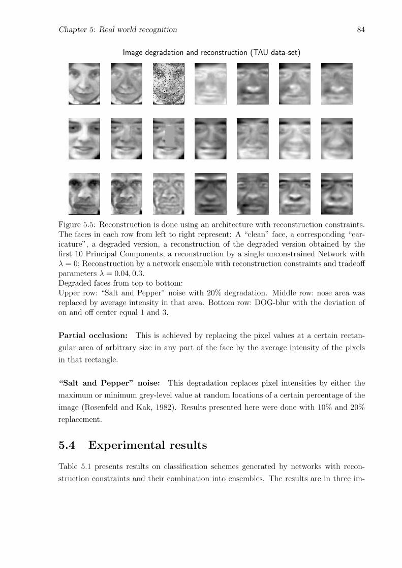
Chapter 5: Real world recognition 84
Image degradation and reconstruction (TAU data-set)
Figure 5.5: Reconstruction is done using an architecture with reconstruction constraints.The faces in each row from left to right represent: A “clean” face, a corresponding “car-icature”, a degraded version, a reconstruction of the degraded version obtained by thefirst 10 Principal Components, a reconstruction by a single unconstrained Network withλ = 0; Reconstruction by a network ensemble with reconstruction constraints and tradeoffparameters λ = 0.04, 0.3.Degraded faces from top to bottom:Upper row: “Salt and Pepper” noise with 20% degradation. Middle row: nose area wasreplaced by average intensity in that area. Bottom row: DOG-blur with the deviation ofon and off center equal 1 and 3.
Partial occlusion: This is achieved by replacing the pixel values at a certain rectan-
gular area of arbitrary size in any part of the face by the average intensity of the pixels
in that rectangle.
“Salt and Pepper” noise: This degradation replaces pixel intensities by either the
maximum or minimum grey-level value at random locations of a certain percentage of the
image (Rosenfeld and Kak, 1982). Results presented here were done with 10% and 20%
replacement.
5.4 Experimental results
Table 5.1 presents results on classification schemes generated by networks with recon-
struction constraints and their combination into ensembles. The results are in three im-

Chapter 5: Real world recognition 85
Classification results for Pentland data-setClassification Low Intermediate High
scheme Resolution Resolution Resolution16× 16 32× 32 64× 64
λ = 0 3.1 2.6 1.5λopt 3.1 1.5 1.0
classificationensemble 2.6 0.5 1.0regressionensemble 2.6 1.0 0.5
PCA 15.9 13.8 17.9
Classification Low Intermediate Highscheme Resolution Resolution Resolution
16× 16 32× 32 64× 64λ = 0 5.1 12.3 16.9λopt 4.6 7.2 11.8
classificationensemble 4.6 8.2 13.3regressionensemble 4.6 8.2 10.3
PCA 22.1 35.4 50.8
Classification Low Intermediate Highscheme Resolution Resolution Resolution
16× 16 32× 32 64× 64λ = 0 5.1 3.6 1.5λopt 3.6 2.6 1.5
classificationensemble 4.1 1.5 1.5regressionensemble 4.1 1.5 0.5
PCA 16.4 14.8 17.9
Classification Low Intermediate Highscheme Resolution Resolution Resolution
16× 16 32× 32 64× 64λ = 0 36.4 13.8 5.6λopt 34.4 11.7 3.6
classificationensemble 33.8 14.9 4.1regressionensemble 32.3 13.3 2.6
PCA 46.7 33.3 26.7
Table 5.1: Percent misclassification rate for Turk-Pentland data-set in three resolutions.Top left: on the “clean” testing set. Top right: Blurred images with a DOG-filter withσ1 = 1 σ2 = 2. Bottom left: Results of partial occlusion around the nose. Bottom right:Results of a “Salt and Pepper” noise of 20% of the image. For 32× 32 resolution, singleunconstrained net with λ = 0 and reconstruction ensemble correspond to initial “weightsB” of Table 5.2. PCA stands for PCA network.
age resolutions with different image degradations. They show that constrained networks
which may not show significant performances difference on tests with original, undegraded
test-set, do show a significant improvement when tested with degraded images. Below,
we highlight some consequences of Table 5.1.
Single PCA network When λ = 1 and the activation functions of the hidden and
output units are linear, the hidden weights of the network span the space of principal
eigenvectors (Section 3.1.2). Classification results for network PCA representations are
presented in Table 5.1 (bottom rows). These results are inferior to other methods and
demonstrate that the first few principal components may be inefficient for classification1.
Ensemble combination Classification ensemble, or voting, is quite common in com-
putational learning theory (Section 2.2). We find that a regression ensemble is superior
to classification ensemble especially in higher image resolutions. We note that for a re-
gression ensemble variance reduction by averaging is achieved when the errors of the
different classifiers are independent. It appears that the use of different λ values leads to
1It is known however, that a larger number of PCA produces improved results (Kirby and Sirovich,1990).
Chapter 5: Real world recognition 86
some independence in misclassification and thus, the regression ensemble produces better
results.
Different image resolutions Generally, the results from the 16 × 16 resolution are
only slightly worse than results with higher resolutions. This resolution is less sensitive to
difference of Gaussians blur, but very sensitive to “Salt and Pepper” noise which produces
significantly worse results. This is a strong indication to the usefulness of multi-resolution
detection as a means to improve performance under various image degradations.
In short, Table 5.1 indicates that reconstruction constraints under regression ensemble
produce more robust results. In the following set of experiments, we consider other
network constraints.
5.4.1 Different architecture constraints and regularization en-sembles
Table 5.2 presents results on different classification schemes that were generated by various
network constraints and regression ensemble combinations. All results were obtained on
the Turk-Pentland data-set with an intermediate (32 × 32) resolution, using networks
trained with two sets of initial random weights A and B.
Unconstrained ensembles The first two rows in Table 5.2 represent two single (con-
ventional) unconstrained networks, corresponding to training with different initial weights
A and B. This serves as a base-line comparison and demonstrates the increased sensitivity
of single networks to image degradation, in particular to blur. Before concentrating on the
effects of additional constraints we note that ensemble without additional constraints (1st
numbered row of Table 5.2) is already significantly better than a single network. Similar
results for the TAU data-set are presented in the second row of Table 5.3.
Reconstruction networks and their ensembles The next two rows (numbered 2
and 3, in Table 5.2) show the variability of the reconstruction ensemble results due to
a different initial set of weights (A and B). Classification results of the reconstruction
ensemble for the TAU data-set are shown in the 3rd row of Table 5.3. For this (more
difficult) data-set, the ensemble of unconstrained networks is always inferior to the en-
semble with reconstruction constraints. The largest difference between the unconstrained
and reconstruction ensembles is observed for blurred images.
The 4th row of Table 5.2 represents the reconstruction ensemble composed from the
networks of two reconstruction ensembles with weights A and B. The main observation

Chapter 5: Real world recognition 87
Different Ensemble Types (Pentland data-set)
Ensembles: Optimal NN Regression Gaussian DOG Occlusion “Salt andType of for ensemble filter filter nose half Pepper noise”
regularization testing on testing σ1 = 1 area face d=0.1 d=0.2constraints: set set σ = 2 σ2 = 2 area
Single unconstrained netwith initial “weights A” 1.0 * 10.3 8.2 1.0 7.2 4.6 10.8Single unconstrained netwith initial “weights B” 2.6 * 12.8 12.3 3.6 8.7 6.2 13.8
1. Ensemble for λ = 0 anddifferent initial weights 1.0 0.5 6.7 7.7 0.5 5.6 2.1 7.22. Reconstruction withinitial “weights A” 2.1 2.1 8.2 4.1 1.5 5.6 6.7 12.8λ : 0.05 0.1 0.3 0.353. Reconstruction withinitial “weights B” 1.5 1.0 8.7 8.2 1.5 6.2 3.1 13.3λ : 0.1-0.3, step 0.054. Reconstruction ensemble withinitial “weights A,B” 1.5 1.5 6.2 4.6 2.1 4.6 4.1 9.7
5. Reconstruction (A+B) andλ = 0 ensembles 1.0 0.5 5.6 4.6 0.5 4.6 2.6 6.7
6. Reconstruction withentropy maximization 1.5 2.1 7.2 4.6 2.6 4.6 4.1 8.7λ : 0.05 - 0.3, step 0.057. Reconstruction and entropymaximization ensembles 1.0 1.5 5.6 3.1 1.5 4.6 4.1 7.2
8. Entropy maximizationλ : 0 - 0.4, step 0.05 0.5 1.5 8.7 4.1 2.1 6.7 3.6 11.39. BCMλ : 0.05 -0.3, step 0.05 2.1 2.6 11.3 5.1 2.1 8.2 4.1 11.8
10. Sum of entropies Aλ : 0.05 0.1 0.2 0.25 0.3 1.5 2.1 8.2 7.7 2.6 3.6 4.1 10.8
11. Sum of entropies Bλ : 0.05 0.1 0.2 0.25 0.3 1.5 2.1 8.2 7.7 2.6 3.6 3.6 13.3
12. Sum of entropies Cλ : 0.05 0.1 0.2 0.25 0.3 0.5 2.1 7.7 7.7 2.1 6.7 2.1 9.7
13. Sum of entropies Dλ : 0.05 - 0.3, step 0.05 1.0 2.1 8.2 6.7 2.1 5.6 3.6 8.7
14. Nonlinear PCAλ : 0-0.3, step 0.1 2.6 3.6 20 21.5 7.6 26.2 51.3 74.4
Table 5.2: Percent classification error for different image corruptions on the Turk-Pentlanddata-set in intermediate (32× 32) resolution. All results are for an ensemble of networksthat includes the indicated λ values. The column optimal NN refers to the single best inthe ensemble λ-network. In the Salt and Pepper experiments, either 10% or 20% of theimage were corrupted. Information that is not relevant for single networks is marked with*.
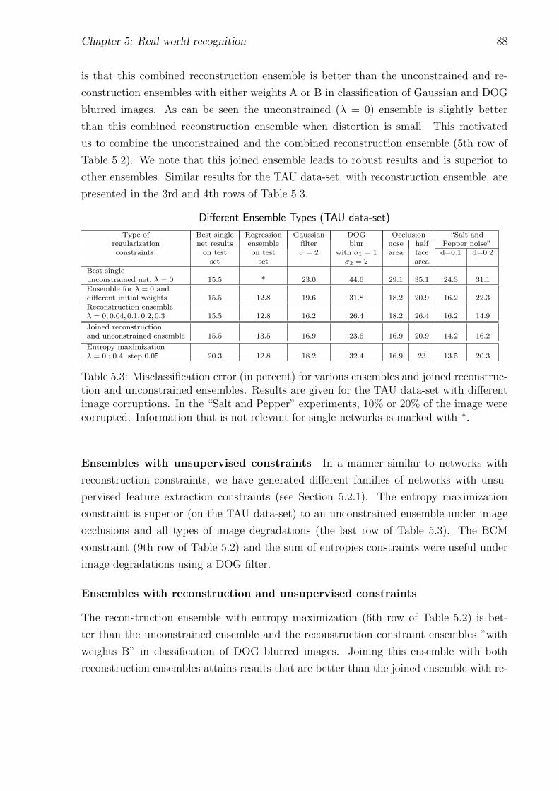
Chapter 5: Real world recognition 88
is that this combined reconstruction ensemble is better than the unconstrained and re-
construction ensembles with either weights A or B in classification of Gaussian and DOG
blurred images. As can be seen the unconstrained (λ = 0) ensemble is slightly better
than this combined reconstruction ensemble when distortion is small. This motivated
us to combine the unconstrained and the combined reconstruction ensemble (5th row of
Table 5.2). We note that this joined ensemble leads to robust results and is superior to
other ensembles. Similar results for the TAU data-set, with reconstruction ensemble, are
presented in the 3rd and 4th rows of Table 5.3.
Different Ensemble Types (TAU data-set)
Type of Best single Regression Gaussian DOG Occlusion “Salt andregularization net results ensemble filter blur nose half Pepper noise”constraints: on test on test σ = 2 with σ1 = 1 area face d=0.1 d=0.2
set set σ2 = 2 areaBest singleunconstrained net, λ = 0 15.5 * 23.0 44.6 29.1 35.1 24.3 31.1Ensemble for λ = 0 anddifferent initial weights 15.5 12.8 19.6 31.8 18.2 20.9 16.2 22.3Reconstruction ensembleλ = 0, 0.04, 0.1, 0.2, 0.3 15.5 12.8 16.2 26.4 18.2 26.4 16.2 14.9
Joined reconstructionand unconstrained ensemble 15.5 13.5 16.9 23.6 16.9 20.9 14.2 16.2
Entropy maximizationλ = 0 : 0.4, step 0.05 20.3 12.8 18.2 32.4 16.9 23 13.5 20.3
Table 5.3: Misclassification error (in percent) for various ensembles and joined reconstruc-tion and unconstrained ensembles. Results are given for the TAU data-set with differentimage corruptions. In the “Salt and Pepper” experiments, 10% or 20% of the image werecorrupted. Information that is not relevant for single networks is marked with *.
Ensembles with unsupervised constraints In a manner similar to networks with
reconstruction constraints, we have generated different families of networks with unsu-
pervised feature extraction constraints (see Section 5.2.1). The entropy maximization
constraint is superior (on the TAU data-set) to an unconstrained ensemble under image
occlusions and all types of image degradations (the last row of Table 5.3). The BCM
constraint (9th row of Table 5.2) and the sum of entropies constraints were useful under
image degradations using a DOG filter.
Ensembles with reconstruction and unsupervised constraints
The reconstruction ensemble with entropy maximization (6th row of Table 5.2) is bet-
ter than the unconstrained ensemble and the reconstruction constraint ensembles ”with
weights B” in classification of DOG blurred images. Joining this ensemble with both
reconstruction ensembles attains results that are better than the joined ensemble with re-
Chapter 5: Real world recognition 89
construction and no constraints ensemble for DOG blurred images (7th row of Table 5.2).
In general, however, merging of ensembles with reconstruction constraints and with no
constraints (λ = 0) leads to more robust results and is superior to the joined reconstruc-
tion and entropy constraints ensemble.
Figure 5.6 summarizes most results of Table 5.2 and compares between different en-
semble averaging schemes and different learning constraints on the original and degraded
images. It shows that the “joined reconstruction ensemble” (pink, fifth bar) performs
better than each reconstruction ensemble from which it is composed. Additional merging
with the unconstrained (λ = 0) ensemble (black, seventh bar), gives a better performance
in most of the cases. The same useful property of the reconstruction ensemble can be
observed when merging reconstruction and entropy maximization ensembles (yellow, sixth
bar). This ensemble is superior under DOG blurred images.
5.5 Saliency detection
This section presents a way to improve recognition of corrupted images using network
generalization ability to reconstruct. Due to the bottleneck structure of the network,
reconstruction is efficient even when images contain a large amount of noise or are partially
occluded by contrast objects. Reconstructed images, which we call prototypes, are able to
recover partially degraded or occluded areas of the input. However, there is a difficulty to
find these degraded areas in the input, or more generally, to define relevance (confidence)
of the image areas. This task is common in artificial intelligence and robotic vision. It is
referred to as a saliency detection or intelligent filtering (Baluja, 1996). The definition of
relevance depends on the desired task and the learning algorithm.
For example, for an autonomous vehicle navigation (Baluja and Pomerleau, 1995) a
saliency map derived from a specific Neural Network representation (see Section 3.1.5)
was designed to highlight significant (salient) regions of the input and deemphasize unim-
portant regions. Their saliency map is based on the difference between an input image
and its prediction by the network from the previous video frame. Below, we present a
saliency map construction for still images that is suitable for the classification task and
uses the hybrid network, which was introduced in Chapter 3.
5.5.1 Saliency map
After training a difference map (image) xd given by the difference between the input
image x and its prototype xp: xd = abs(x − xp), can be used for extracting unreliable
areas (areas with a large noise or unexpected objects) in the input image. Due to the
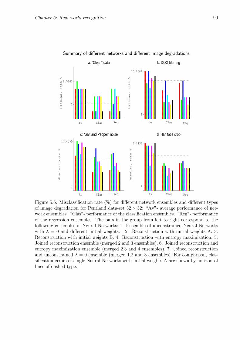
Chapter 5: Real world recognition 90
Summary of different networks and different image degradations
1
2.5641
a: "Clean" dataMisclas. rate %
Av Clas Reg
1
10.2564
b: DOG blurring
Misclas. rate %
Av Clas Reg
1
17.4359
c: "Salt and Pepper" noise
Misclas. rate %
Av Clas Reg
1
9.7436
d: Half face cropMisclas. rate %
Av Clas Reg
Figure 5.6: Misclassification rate (%) for different network ensembles and different typesof image degradation for Pentland data-set 32 × 32: “Av”- average performance of net-work ensembles. “Clas”- performance of the classification ensembles. “Reg”- performanceof the regression ensembles. The bars in the group from left to right correspond to thefollowing ensembles of Neural Networks: 1. Ensemble of unconstrained Neural Networkswith λ = 0 and different initial weights. 2. Reconstruction with initial weights A. 3.Reconstruction with initial weights B. 4. Reconstruction with entropy maximization. 5.Joined reconstruction ensemble (merged 2 and 3 ensembles). 6. Joined reconstruction andentropy maximization ensemble (merged 2,3 and 4 ensembles). 7. Joined reconstructionand unconstrained λ = 0 ensemble (merged 1,2 and 3 ensembles). For comparison, clas-sification errors of single Neural Networks with initial weights A are shown by horizontallines of dashed type.

Chapter 5: Real world recognition 91
bottleneck structure of the network, the output of the reconstruction layer has to be better
for recognition than the original signal, in areas where xd is large, i.e., the original signal
x is messy. Thus, we propose before recognition to replace the original image x by the
image xn using a saliency map Φ(xd):
xn = Φ(xd)x+ (1− Φ(xd))xp, (5.5.1)
where all operations are pixel-wise.
We have constrained a saliency map Φ(xd) to be a decreasing function, such that
Φ(0) = 1 and have considered two types of saliency maps. The first type of saliency maps
is given by: Φ(x) = exp(−µx2) and parameter µ, tuned to µ = 0.9. The second saliency
map was taken as:
Φ(x) =
1 if x < x0.5 otherwise
where a threshold x was adjusted to 0.3. Figure 5.7 shows examples of the xn images
obtained using two saliency maps. Classification was improved for some types of the
Saliency map construction
Input Reconstruction Difference
Saliency Reconstruction Saliency Reconstructionmap-1 with map-1 map-2 with map-2
Figure 5.7: Reconstruction using saliency maps for network with reconstruction con-straints and trade-off parameter λ = 0.04 (TAU data-set). The white pixels of the firstmap (map-1) correspond to intensity equal to 1 and black to zero intensity. In map-2 thewhite pixels have intensity equal to 0.5 and black 0.
degradation process, especially for “Salt and Pepper” noise (Tables 5.4–5.5). For other

Chapter 5: Real world recognition 92
Recognition using saliency maps (Pentland data-set)
Types of Regression Ensemblesdegradation Unconstrained Reconstruction A Reconstruction B Joined
“Salt and Pepper”noise with d = 0.1input 1.5 2.1 3.1 1.0map-1 1.5 3.1 3.1 1.0map-2 1.5 3.1 4.1 1.5“Salt and Pepper”noise with d = 0.2input 7.2 11.3 11.3 6.7map-1 2.6 4.6 4.1 3.6map-2 2.6 4.6 5.6 3.6“Salt and Pepper”noise with d = 0.3input 25.1 26.2 30.8 23.6map-1 11.3 13.3 13.3 11.8map-2 12.8 14.9 15.9 12.3“Right eye”with ν = 3input 3.1 1.5 2.1 2.1map-1 3.1 1.5 2.1 0.5map-2 2.6 2.1 2.6 1.0“Half face”with ν = 3input 15.9 26.2 22.1 18.5map-1 16.9 26.2 22.1 16.9map-2 16.9 25.6 19.5 17.4“DoG 1-2”input 7.7 4.1 9.2 4.6map-1 7.7 3.6 9.7 4.1map-2 8.2 3.6 8.7 5.6
Table 5.4: Percent misclassification error results for images obtained using two types ofsaliency maps. Reconstruction ensembles A and B correspond to training with weightsA and B. In contrast with reconstruction ensembles A–B in Table 5.2 (2-3 rows), theycontain also one unconstrained network (λ = 0). Rows marked with “input” show standfor the input degraded images. Pentland data-set at 32× 32 resolution.

Chapter 5: Real world recognition 93
Recognition using saliency maps (TAU data-set)
Types of Regression Ensemblesdegradation Unconstrained Reconstruction Joined
“Salt and Pepper”noise with d = 0.1input 16.2 16.9 13.5prototype 23.0 16.2 14.9map-1 14.2 14.2 12.8map-2 14.2 14.9 12.2“Salt and Pepper”noise with d = 0.2input 25.0 20.3 20.3prototype 31.1 18.2 20.3map-1 18.2 14.2 12.8map-2 18.2 15.5 12.8“Salt and Pepper”noise with d = 0.3input 37.8 31.8 31.1prototype 43.2 31.1 32.4map-1 25.7 18.9 20.3map-2 21.6 17.6 18.9“Right eye”with ν = 3input 14.2 15.5 13.5prototype 14.9 14.9 13.5map-1 14.2 15.5 13.5map-2 13.5 15.5 13.5“Half face”with ν = 3input 43.9 36.5 34.5prototype 43.2 41.9 36.5map-1 42.6 36.5 34.5map-2 41.9 35.8 36.5“DoG 1-2”input 31.8 26.4 23.6prototype 33.1 26.4 27.0map-1 32.4 27.7 24.3map-2 33.1 27.0 25.0
Table 5.5: Percent misclassification error results for images obtained using two types ofsaliency maps. Rows marked by “prototype” stand for the reconstructed images (TAUdata-set).

Chapter 5: Real world recognition 94
types of image degradation, classification improvement was not significant. To enforce
the efficiency of the saliency map, in the experiments with partially occluded images, the
occluded region was enhanced by multiplying the average intensity over the occluded area
by some factor ν.
5.6 Conclusions
We have shown that constraints on the properties of the low-dimensional internal repre-
sentation of the images, such as entropy maximization, BCM and the sum of entropies,
are useful and can be considered in conjunction with reconstruction constraints, to im-
prove generalization for classification. It was further shown that an averaging of Neural
Networks with different constraint strengths is preferable to a simple choice of the optimal
regularized network parameters. The best classification results were obtained by merging
the ensemble with reconstruction constraints and the unconstrained, λ = 0 ensemble.
Reconstruction constraints significantly improve classification results under partial
occlusion, lossy compression, “Salt and Pepper” noise and some image blur operations. In
addition, we have shown that via saliency maps, reconstruction can deemphasize degraded
regions of the input, thus leading to classification improvement under “Salt and Pepper”
noise. In the next chapter, we investigate the influence of the reconstruction constraints
on image recognition under a wide family of image blur and consequent deblur operations.

Chapter 5: Real world recognition 95
5.7 Appendix to Chapter 5: Hidden representation
exploration
Image recognition improvement is based on the extraction of a good hidden data rep-
resentation. Although recognition performance is a single reliable measure that allows
one to judge the hidden representation quality, it may be interesting to consider some
statistics of the hidden layer units. Statistics of the hidden unit activities characterize
the data distribution after projection on the hidden weight directions. Some properties
of the hidden representation are presented below.
In Figures 5.8–5.9, the hidden unit activities per classes and different bias constraints
are shown. As can be seen, in both networks images of the same class excite similar
activation patterns in their hidden space and at the same time there is a big difference
between patterns corresponding to different classes. It is clear that such a representation
has to be good for recognition. However, from the observations it is difficult to decide
which type of constraints is preferable.
The pdfs of the hidden unit activities are presented in Figure 5.10. As can be seen,
they are multi-modal for unconstrained network and multi-modal or super-Gaussian for
reconstruction network. Both these properties are useful for recognition (Chapter 4).
Another way to get some impression about hidden layer structure is to look at the
hidden weights as images (Figure 5.11). We note, however, that network ensemble hidden
representation is not well defined.
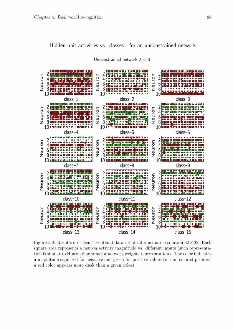
Chapter 5: Real world recognition 96
Hidden unit activities vs. classes - for an unconstrained network
Unconstrained network λ = 0
2468
10class−1
Ne
uro
n 2468
10class−2
Ne
uro
n 2468
10class−3
Ne
uro
n
2468
10class−4
Ne
uro
n 2468
10class−5
Ne
uro
n 2468
10class−6
Ne
uro
n
2468
10class−7
Ne
uro
n 2468
10class−8
Ne
uro
n 2468
10class−9
Ne
uro
n
2468
10class−10
Ne
uro
n 2468
10class−11
Ne
uro
n 2468
10class−12
Ne
uro
n
2468
10class−13
Ne
uro
n 2468
10class−14
Ne
uro
n 2468
10class−15
Ne
uro
n
Figure 5.8: Results on “clean” Pentland data set at intermediate resolution 32×32. Eachsquare area represents a neuron activity magnitude vs. different inputs (such representa-tion is similar to Hinton diagrams for network weights representation). The color indicatesa magnitude sign: red for negative and green for positive values (in non colored printers,a red color appears more dusk than a green color).

Chapter 5: Real world recognition 97
Hidden unit activities vs. classes - for a reconstruction network
Reconstruction network λ = 0.3
2468
10class−1
Ne
uro
n 2468
10class−2
Ne
uro
n 2468
10class−3
Ne
uro
n
2468
10class−4
Ne
uro
n 2468
10class−5
Ne
uro
n 2468
10class−6
Ne
uro
n2468
10class−7
Ne
uro
n 2468
10class−8
Ne
uro
n 2468
10class−9
Ne
uro
n
2468
10class−10
Ne
uro
n 2468
10class−11
Ne
uro
n 2468
10class−12
Ne
uro
n
2468
10class−13
Ne
uro
n 2468
10class−14
Ne
uro
n 2468
10class−15
Ne
uro
n
Figure 5.9: Results on “clean” Pentland data set at intermediate resolution 32× 32.

Chapter 5: Real world recognition 98
Pdf’s of hidden unit activities
Unconstrained network λ = 0
neuron−1 neuron−2 neuron−3 neuron−4 neuron−5
neuron−6 neuron−7 neuron−8 neuron−9 neuron−10
Reconstruction network λ = 0.3
neuron−1 neuron−2 neuron−3 neuron−4 neuron−5
neuron−6 neuron−7 neuron−8 neuron−9 neuron−10
Figure 5.10: Hidden unit activity pdfs - for unconstrained λ = 0 and reconstructionnetwork λ = 0.3 for “clean” Pentland data set at intermediate resolution 32× 32.
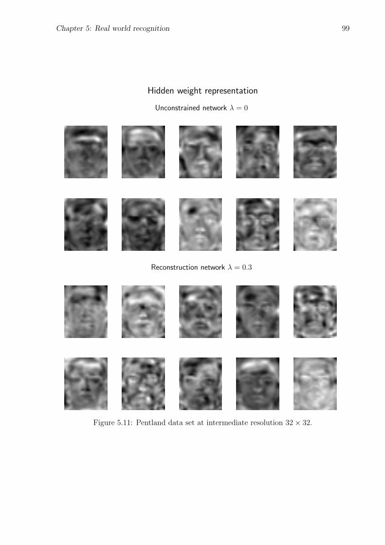
Chapter 5: Real world recognition 99
Hidden weight representation
Unconstrained network λ = 0
Reconstruction network λ = 0.3
Figure 5.11: Pentland data set at intermediate resolution 32× 32.

Chapter 6
Blurred image recognition
This chapter studies a case where the required generalizations are for data which may
be “far” from data in the training set, namely data with a different distribution than
the training set. In the previous chapter, we considered unsupervised and particularly
reconstruction constraints, as a mechanism to impose useful bias during training. We
have shown that these constraints improve generalization performance for various image
degradations, such as “Salt and Pepper” noise, low resolution and partial occlusion. How-
ever, sensitivity to image blur was still too high. This chapter is devoted to performance
improvement under various types of image blur.
6.1 Methodology
Recognition of blurred images requires a substantial amount of training data processed
by different blur operators. Unfortunately, such data is not available, and therefore, an
alternative way to solve the problem is to impose a priori information about possible
degradation transformations.
For example, in the character recognition problem, the possible transformations are
geometrical, such as shift, rotation and scaling (Simard et al., 1992; Baird, 1990). The
regularization there appears as the invariance tangent prop constraints in the form of
the penalty term to the cost function or using the distortion model, i.e. by data driven
regularization (Section 2.3.2).
We choose to add Gaussian blurred images to the training set as a representative of all
blur operations and recognition is done on a wide variety of blur operations. We further
propose to enforce reconstruction of blurred images to either their copy or to the original
non-blurred images. Such training causes the hidden representation to become insensitive
to blur operation.
Another obvious way to improve classification of the blurred images is to restore the
100
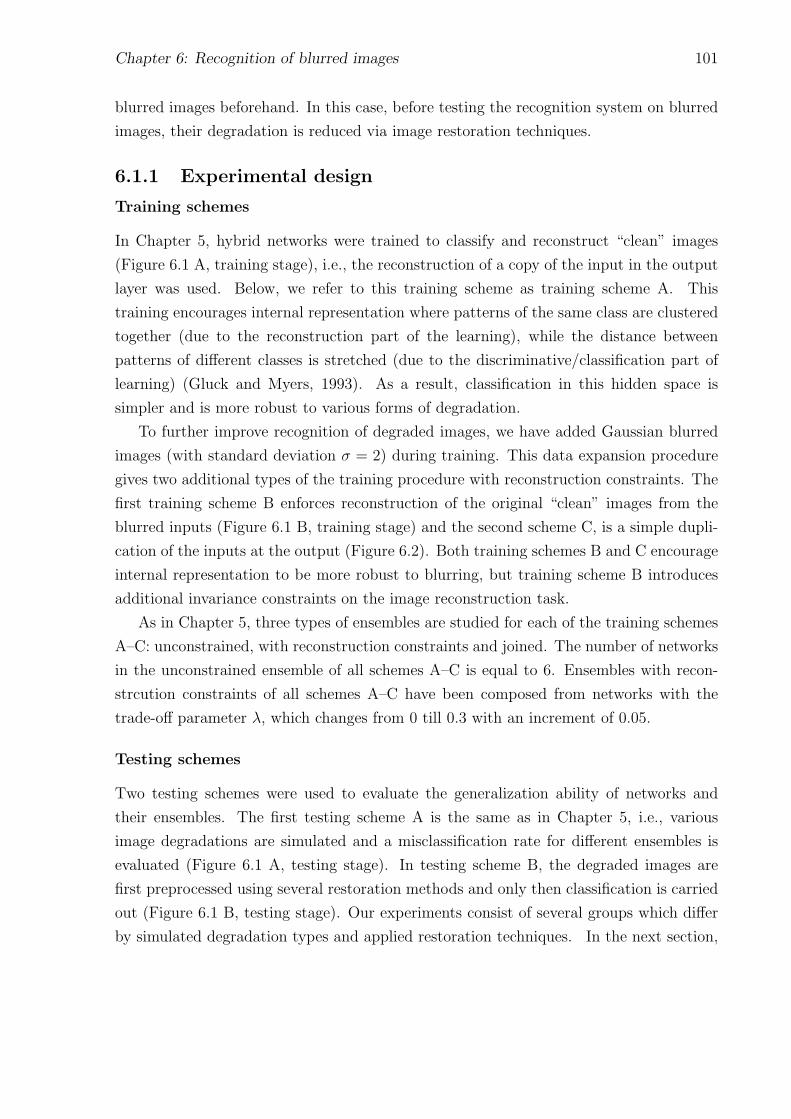
Chapter 6: Recognition of blurred images 101
blurred images beforehand. In this case, before testing the recognition system on blurred
images, their degradation is reduced via image restoration techniques.
6.1.1 Experimental design
Training schemes
In Chapter 5, hybrid networks were trained to classify and reconstruct “clean” images
(Figure 6.1 A, training stage), i.e., the reconstruction of a copy of the input in the output
layer was used. Below, we refer to this training scheme as training scheme A. This
training encourages internal representation where patterns of the same class are clustered
together (due to the reconstruction part of the learning), while the distance between
patterns of different classes is stretched (due to the discriminative/classification part of
learning) (Gluck and Myers, 1993). As a result, classification in this hidden space is
simpler and is more robust to various forms of degradation.
To further improve recognition of degraded images, we have added Gaussian blurred
images (with standard deviation σ = 2) during training. This data expansion procedure
gives two additional types of the training procedure with reconstruction constraints. The
first training scheme B enforces reconstruction of the original “clean” images from the
blurred inputs (Figure 6.1 B, training stage) and the second scheme C, is a simple dupli-
cation of the inputs at the output (Figure 6.2). Both training schemes B and C encourage
internal representation to be more robust to blurring, but training scheme B introduces
additional invariance constraints on the image reconstruction task.
As in Chapter 5, three types of ensembles are studied for each of the training schemes
A–C: unconstrained, with reconstruction constraints and joined. The number of networks
in the unconstrained ensemble of all schemes A–C is equal to 6. Ensembles with recon-
strcution constraints of all schemes A–C have been composed from networks with the
trade-off parameter λ, which changes from 0 till 0.3 with an increment of 0.05.
Testing schemes
Two testing schemes were used to evaluate the generalization ability of networks and
their ensembles. The first testing scheme A is the same as in Chapter 5, i.e., various
image degradations are simulated and a misclassification rate for different ensembles is
evaluated (Figure 6.1 A, testing stage). In testing scheme B, the degraded images are
first preprocessed using several restoration methods and only then classification is carried
out (Figure 6.1 B, testing stage). Our experiments consist of several groups which differ
by simulated degradation types and applied restoration techniques. In the next section,

Chapter 6: Recognition of blurred images 102
Experimental design schemesA B
clean imageClass label
clean image
Classification
Reconstruction
Training stage
Training stage
clean image clean image
Blurred image clean image
Reconstruction
Class label
Classification
Reconstruction
A B
Blurred image
Testing stage
Class
?
Testing stage
RestorationClass
?
Degraded image Restored image
Figure 6.1: (A): In the training stage, networks are trained to classify and reconstruct“clean” images. In the testing stage A, generalization ability to classify artificially de-graded images is tested; (B): Artificially blurred images are added to the training stage.Networks are trained to classify images and reconstruct their “clean” prototypes. In thetesting stage B, restoration preprocessing is used before recognition schemes.
we review image degradation operations and restoration methods which we apply.
6.2 Image degradation
Usually degradation process is modeled as both a space-invariant blurring with a convo-
lution operator h and a corruption with an additive noise n:
g = h ∗ f + n, (6.2.1)
where f is the original image. The major known causes for image blur are misfocus, camera
jitter, object motion and atmospheric turbulence. These types of blur lead to a low pass
operation on the image. Of particular interest is a difference of Gaussians (DOG) filter,
which is a band-pass filter, and is known to be present in early mammal vision (Kandel
and Schwartz, 1991). This operator is equivalent to simultaneous image smoothing and
enhancement. A third family of image filters is the high pass filter which leads to image
sharpening. This filter is common in medical imaging, industrial inspection and military

Chapter 6: Recognition of blurred images 103
Training scheme C
Training stage
clean image clean image
Blurred image clean image
Reconstruction
Class label
Classification
Reconstruction
Figure 6.2: In the training stage, the network is trained to classify and reconstruct “clean”and blurred images. Reconstruction is a copy of the input in the output sublayer.
applications. The presence of noise in images is inevitable. It may be a result of image
generation, recording, transmission, etc. Noise corruption complicates image acquisition
and even a small amount of it is harmful for restoration of blurred images. We consider
two types of additive noise: Gaussian white noise and pulse noise. We limit ourselves to
Gaussian noise that acts independently on each pixel, with zero mean and some variance σ.
Pulse noise (otherwise called “Salt and Pepper” noise) replaces pixel intensities by either
the maximum or minimum grey-level values with some probability (Rosenfeld and Kak,
1982), producing separate high contrast black-and-white points. This noise is common in
video transmission.
6.2.1 Main filters
Filtering may be done both in the frequency and spatial domains. Convolution in the
spatial domain is equivalent to multiplication of the Fourier transforms of the image and
the filter in the frequency domain. In each particular case we indicate in which domain
filtering is done and represent point spread function or its Fourier transform (referred to
as a transfer function) as required. Examples of images with various degradations are
shown in Figure 6.3.
Ideal filters
Ideal filters represent a class of frequency domain filtering that are easy to simulate.
Transfer functions of these filters are radially symmetric about the origin and though
they are not physically realizable, they are widely used in image processing for comparing
the behavior of different types of filters. The name ideal indicates that some specified

Chapter 6: Recognition of blurred images 104
Degraded Images
original a b c d
e f g h i
Figure 6.3: a) Result of Gaussian noise with σ = 2; b) Result of pulse noise with density20%; c) Result of replacement of the nose area with average intensity over this area; d)Result of the root filter with α = 0.6; e) Result of the out-of-focus filter with the blurradius R = 5; f) Motion blur with blur propagation on 7 pixels; g) Result of Gaussianblur with σ = 2; h) Result of the DOG filter with on and off centers equal to σ1 = 1 andσ2 = 2 i) Result of the ideal high pass filter with cutoff w = 3
frequencies are completely eliminated. Depending on the eliminated frequencies ideal low,
band and high pass filters are known (Gonzalez and Wintz, 1993). A transfer function of
the ideal filter in the frequency domain (u, v) is given by the expression:
H(u, v) =
1 if (u, v) ∈ D0 otherwise,
where the area of the unchanged frequencies D is:
a)√u2 + v2 ≤ W ?, b)
√u2 + v2 ≥ W 0, c) W ? <
√u2 + v2 < W 0,
for low, high and band-pass filters respectively, W ?, W 0 are called cutoff frequencies.
Motion blur
Motion blur is a form of image degradation that may degrade recognition performance
(Figure 6.3f). It is due to a relative motion between the camera and the object. Assuming
that a relative camera motion is horizontal and uniform and the total displacement during
the exposure time T is a, the transfer function H(u, v) (Gonzalez and Wintz, 1993) is
given by:
H(u, v) =T
πuasin(πua) exp(−πiua). (6.2.2)

Chapter 6: Recognition of blurred images 105
H vanishes at values of u given by u = na, where n is a nonzero integer. In general, the
amplitude of H(u, v) is characterized by periodic lines of zeros, which are orthogonal to
the direction of motion and are spaced at intervals of 1a
in both sides of the frequency
plane.
Out-of-focus blur
The point spread function (PSF) of a defocused lens with a circular aperture is approxi-
mated by the cylinder whose radius R depends on the extent of the focus defect (Cannon,
1976):
h(x, y) =
1
πR2 if x2 + y2 ≤ R2
0 otherwise,
where R is the “blur radius” which is proportional to the extent of defocusing. The Fourier
transform of h(x, y) in this case is H(u, v) = J1(πRr)/(πRr), where J1 is the first-order
Bessel function and is characterized by “almost-periodic” circles with zero valued H(u, v).
This occurs for r satisfying: 2πRr = 3.83, 7.02, 10.2, 13.3, 16.5 . . .
The well-defined structure of H(u, v) zeros in the case of motion and misfocus blur is
used for the identification of the blur parameter (Cannon, 1976; Fabian and Malah, 1991)
for the purpose of image restoration. However, these methods are sensitive to noise. To
overcome this drawback, some preprocessing stage for noise reduction and estimation were
used (Fabian and Malah, 1991). An example of a misfocus image with blur radius R = 5
is shown in Figure 6.3e.
Gaussian blur
Gaussian blur may be caused by atmospheric and optical blur. It is known that the
eyes’ lenses cause such blur. Computer tomography images also suffer from Gaussian blur
(Kimia and Zucker, 1993). The Gaussian convolution filter written in polar coordinates
h(r, φ) in the spatial domain is given by:
h(r, φ) = Cσ−2 exp(−r2
2σ2), (6.2.3)
where C is a normalization constant. The lack of zero crossing of the Gaussian filter in the
frequency domain makes its identification very difficult. Moreover, Gaussian deblurring
is numerically unstable (Humel et al., 1987; Kimia and Zucker, 1993). An example of an
image blurred by this filter with σ = 2 is shown in Figure 6.3g.
Chapter 6: Recognition of blurred images 106
DOG filter
The difference of Gaussian (DOG) filter is a good approximation to the circular symmetric
Mexican hat type receptive fields (center-surround) found in early mammal vision (Marr,
1982; Kandel and Schwartz, 1991). It performs a band-pass filter that is the result of
applying the Laplacian operator ∇2 to an image which is blurred with a Gaussian filter.
The zero-crossings of the resulting convolved image are commonly used for edge detection
and segmentation. The DOG filter written in polar coordinates is described by:
h(r, φ) = Cσ−21 exp(
−r2
2σ21
)− Cσ−22 exp(
−r2
2σ22
), (6.2.4)
where σ1 < σ2 and are the standard deviations of the on and off center (positive and
negative Gaussians). An image blurred with a DOG filter is shown in Figure 6.3h.
Root filter
Root filter is commonly used for image enhancement and deblurring (Jain, 1989). It affects
the magnitude of the frequency response of an image V as given by: ‖ V ‖=‖ V ‖α . For
small values of α < 1, it acts as a high pass filter, increasing the ratio between amplitudes
in the high and low frequencies. An image enhanced with a root filter (α = 0.6) is shown
in Figure 6.3d.
6.2.2 Other types of degradation
Noise
We consider two types of additive noise: Gaussian white noise and pulse noise. Gaussian
white noise is commonly used to model sensor noise and quantization process. We limit
ourselves to Gaussian noise that acts independently on each pixel with zero mean and
some variance σ2 (Figure 6.3a). Pulse noise replaces pixel intensities by either the
maximum or minimum grey-level value with some probability (Rosenfeld and Kak, 1982),
producing separate high contrast black-and-white points. This explains why pulse noise
is called otherwise ”Salt and Pepper” noise. Pulse noise often appears during TV image
transmission (Figure 6.3b).
Occlusion
Occlusion occurs as a result of motion, when two or more objects touch or overlap one
another. Another cause for occlusion in 2D images is the change of viewpoint, when
part of an object is occluded by another one. We simulate occlusion by replacing pixel

Chapter 6: Recognition of blurred images 107
intensities at a certain rectangular area in any part of the image by some constant intensity
in that rectangle (Figure 6.3c). A level of occlusion is characterized by a factor ν to the
average intensity of an occluded area.
6.3 Image restoration
Image restoration refers to the problem of recovering an image from its blurred and noisy
version, using some a priori knowledge of the degradation phenomenon and the image
nature. It is well-known that the restoration problem is an ill-posed problem (Gonzalez
and Wintz, 1993; Jain, 1989; Stark, 1987), i.e. a small noise in the observed image results
in an unbounded perturbation in the solution. This instability is often addressed by
a regularization approach (Tikhonov and Arsenin, 1977; Katsaggelos, 1989; Sezan and
Tekalp, 1990; Rudin et al., 1992; You and Kaveh, 1996) that includes restricting the set
of admissible solutions and introducing some a priori knowledge about the image and the
degradation model.
6.3.1 MSE minimization and regularization
Assuming the blur operator H is known, a natural criterion for estimating an original
pixel image f from an observed pixel image g in the absence of any knowledge about
noise, is to minimize the difference between the observed image and a blurred version of
the restored image:
minf
M(f) = minf‖ g −Hf ‖2. (6.3.5)
Often, gradient or conjugate gradient descent methods are used for M(f) minimization
(Katsaggelos, 1989; Sezan and Tekalp, 1990). An application of the gradient method to
the minimization problem (6.3.5) produces the following iterative scheme:
fk+1 = fk + β(Htg −HtHfk), f0 = 0. (6.3.6)
When the blur matrix H is nonsingular and β is sufficiently small, the iterative scheme
converges to the f = H−1g. This solution is known as the inverse filter method. In the
frequency domain, it corresponds to the following estimation of the ideal image frequency
response:
F (u, v) =G(u, v)
H(u, v). (6.3.7)
As mentioned before, blur such as motion or defocusing leads to a singular H matrix. In
this case, the above optimization method yields an iterative scheme that converges to the

Chapter 6: Recognition of blurred images 108
minimum norm least square solution H+g of Eq. 6.3.5 (Katsaggelos, 1989; Jain, 1989),
where H+ is the generalized inverse of matrix H.
In the presence of noise the iterative algorithm converges to H+gb + H+n (where gb
is a blurred image without noise interference) and thus contains noise filtered by the
pseudo-inverse matrix. Often, H is a low-pass filter, therefore, the noise is amplified and
the obtained solution may be very far from the desired one.
To overcome this sensitivity to noise, some a priori information about the noise or
the ideal image is often introduced as a quantitative constraint that replaces an ill-posed
problem by a well-posed one. This method is called regularization. The most well known
regularization methods (Tikhonov and Arsenin, 1977; Sezan and Tekalp, 1990) have a
general formulation as a minimization of the function:
L(f) =‖ Hf − g ‖2 +α ‖ Cf ‖2,
where the regularization operator C is chosen to suppress the energy of the restored image
in the high frequencies, that is equivalent to an assumption about the smoothness of the
original image in the spatial domain. Since usually the H filter is a low pass filter, in
order to obtain the smooth original image, the regularization operator C is taken to be
a Laplacian ∇ · ∇f , where ∇ – is a differential operator. A regularization parameter α
may be known a priori or estimated, but theoretically it is inversely proportional to the
signal to noise ratio (SNR).
Although regularization of the MSE criterion with smoothness constraint ‖ Cf ‖ is
the basis for most of the work in image restoration, it often leads to unacceptable ringing
artifacts around sharp intensity transitions. This effect is due to image blurring around
lines and edges. Some solution to this problem is given by the following functional mini-
mization (Katsaggelos, 1989):
L(f) =∑
x∈Ω
[g(x)− h(x) ∗ f(x)]2 + λ∑
x∈Ω
ω(x)[c(x) ∗ f(x)]2. (6.3.8)
The first term in (6.3.8) represents the fidelity of the restored image with respect to
an observation and the second represents a smoothness constraint, ∗ – is a convolution
operator. The space adaptivity is achieved through the introduction of the weight function
ω. The weight function ω is set to be small around the edge areas, larger near the smooth
areas and usually is taken in practice as the inverse of the local variance of the image.
The space adaptivity approach has been extended to the case of an unknown blur
operator (You and Kaveh, 1996; Chan and Wong, 1997). The method incorporates a
priori knowledge about the image and the point spread function (PSF) simultaneously. It
proceeds by minimizing the cost function, which consists of a restoration error measure
Chapter 6: Recognition of blurred images 109
and two regularization terms for the image and the blurring kernel; under constraints on
the blur filter energy.
You et al. (You and Kaveh, 1996) formulate the problem as a minimization of the
function dependent on the discrete image and filter values (2D image and filter functions
are quantized on the grid):
L(f, h) =∑
x∈Ω
ω(x)[g(x)− h(x) ∗ f(x)]2 +
λ1
∑
x∈Ω
ω1(x)[c1(x) ∗ f(x)]2 + λ2
∑
x∈Ω
ω2(x)[c2(x) ∗ h(x)]2 (6.3.9)
In (6.3.9) the first term is responsible for the image fidelity and the second and third terms
represent smoothing constraints on the image and the blur filter, respectively. Smoothness
is introduced adaptively via the weights ω1(x) and ω2(x).
Though the gradient descent method is commonly applied for minimization, an al-
ternating minimization (AM) algorithm is used, which is a particular realization of the
coordinate descent method (Luenberger, 1989). The filter and the image are considered
as dual variables. The algorithm alternately minimizes a cost function by descending with
respect to the filter or the image, while fixing the dual variable. In every alternating step,
a quadratic cost function L(f, h|f) or L(f, h|g) is minimized by the conjugate gradient
method. We note that this formulation is equivalent to minimization of a functional:
L(f ,h) =‖ ω(h ∗ f − g) ‖2L2 +λ1 ‖ √ω1C1 ∗ f ‖2L2 +λ2 ‖ √ω2C2 ∗ h ‖2L2 ,
where f and h are image and blur kernel 2D real functions and ‖ · ‖L2 is an L2 – norm.
Regularization with another form of constraint has been considered in (Chan and
Wong, 1997), where the problem is formulated as a minimization of the functional:
L(f ,h) =‖ h ∗ f − g ‖2L2 +α1
∫
Ω|∇f |dx + α2
∫
Ω|∇h|dx. (6.3.10)
The proposed method is called total variation blind deconvolution (TV regularization).
In Eq. (6.3.10) the regularization term has the form∫
Ω |∇f |dx, called a total variation
(TV) norm (Rudin et al., 1992). It follows the idea that the image consists of the smooth
patches, instead of being smooth everywhere, thus providing better recovering of image
edges.
6.3.2 Image restoration in the frequency domain
All the restoration methods considered up to this point were derived in the space domain,
though historically the first methods were designed in the frequency domain. Herein we
survey briefly the most widely spread frequency domain restoration methods.
Chapter 6: Recognition of blurred images 110
Wiener filter
A fundamental result in filtering theory used commonly for image restoration is a Wiener
filter. Wiener filtering has been successfully used to filter images corrupted both by noise
and blurring. This filter gives the best estimate of the object from the observations in
the MSE sense. The Wiener filter frequency response is given as (Jain, 1989):
HW =H?Sff
‖ H ‖2 Sff + Sηη=Sgg − SηηHSgg
. (6.3.11)
In the case where only one observation is available, Sff and Sgg are power spectrums of
ideal and observed images, respectively, and Sηη is a power spectrum of the noise. Since
the phase of the Wiener filter coincides with the phase of the inverse filter, it does not
compensate for phase distortions due to noise in the observations.
In the absence of the blurring, the Wiener filter becomes:
HW =Sff
Sff + Sηη=
snr
snr + 1, (6.3.12)
where snr = Sff/Sηη is a signal-to-noise ratio. In practice, snr is defined as a ratio
between variances of the blurred image and the noise (or 10 log10 snr, if signal-to-noise
ratio is measured in Db) .
This filter (6.3.12) is called the Wiener smoothing filter. It suppresses all frequency
components in which the signal-to-noise ratio is small and does not change the frequency
components when snr is large (snr 1). For images, Sff is usually very small for high
frequencies, therefore the noise smoothing filter is a low pass filter. Another marginal
case is the absence of noise, in which the Wiener filter coincides with the inverse filter
HW = H−1. Since the blurring process is usually a low pass filter, the Wiener filter acts
in this case as a high pass filter.
In the presence of noise and blur, the Wiener filter achieves a compromise between
low-pass noise smoothing and high-pass inverse filtering, resulting in a band-limited filter.
It is clear, nevertheless, that the Wiener filter is also unstable (like the inverse filter), if
the frequency response is zero or close to it.
Inverse and pseudo-inverse filters
As has been already mentioned, in the case of the noise absence, the Wiener filter becomes
an inverse one and requires stabilization. A standard stabilized version of the inverse filter
is described by the following equation:
H−1(w1, w2) =
1
H(w1,w2)if H(w1, w2) ≥ ε1
0 otherwise
Chapter 6: Recognition of blurred images 111
Instead we have used the next version of the pseudo-inverse filter in our simulations
H−1(w1, w2) =
1H(w1,w2)
if H(w1, w2) ≥ ε11
H(w1,w2)+ε2otherwise
The choice of the ε1 and ε2 parameters defines the quality of the deblurred image. In our
simulations, they have been chosen by trial once for all the data set. It is known that
great care must be taken to obtain approximate solutions that achieve the proper balance
between accuracy and stability. (Stark, 1987). Another nonlinear deblur filter is a root
filter (see Section 6.2.1) that is also used for image enhancement.
6.3.3 Denoising
Denoising may be considered a particular restoration method when the PSF of the blur
operator is a delta function. Thus, some of the methods described above are appropriate
for denoising (Rudin et al., 1992; You and Kaveh, 1996). We also consider two examples
of the rank algorithms (Yaroslavsky and Eden, 1996). Rank algorithms are especially
designed for noise reduction. They are based on the statistics extracted from the vari-
ational row, that is a sequence of central pixel and its neighbors, ranked in increasing
order of their intensities. Different definitions of the neighborhood and variational rank
statistics lead to diverse rank algorithms. Rank statistics may be also obtained from local
histograms and are rather computationally efficient, when applied recursively. The main
advantage of the rank algorithms is local adaptivity. Different denoising algorithms may
be also applied in the cascade.
First, we consider an averaging technique, called peer group averaging (PGA), in which
a central pixel intensity is replaced by an average intensity of some predefined neighboring
pixels, which are closest by intensity value. The number of pixels over which averaging is
performed is called the peer group size and it controls the amount of smoothing.
The second method – the median filter, replaces the gray level intensity of each pixel
by the median of its neighboring pixel intensities. This method is particularly effective
when the noise is spike-like. It is nonlinear, is very robust and preserves edge sharpness.
6.4 Results
Our experiments have shown that training with both schemes B and C (see Section 6.1.1)
leads to recognition improvement compared with the training scheme A. We have also
observed that scheme B is superior to scheme C, but the difference between them is in-
significant. Therefore, below we concentrate on ensembles obtained by using two training

Chapter 6: Recognition of blurred images 112
schemes A and B, and postpone with summary comparison results for all three schemes
until Section 6.4.6. All experiments are carried out on the TAU facial data-set.
6.4.1 Image filtering
In the first group of experiments, the abilities of different ensembles to classify images
processed by ideal and some typical low, band and high pass filters have been compared.
Classification results are presented in Table 6.1 and some degraded images in Figure 6.3.
Classification results for filtered dataTypes of Training scheme A Training scheme B
corruption with extra blurred imagesUnconstrained Reconstruction Joined Unconstrained Reconstruction Joined
λ = 0 ensemble ensemble λ = 0 ensemble ensemble”Clean data” 12.8 12.8 13.5 9.5 10.8 8.8
Ideal low-pass 15.5 14.2 13.5 9.5 10.1 9.5cutoff w = 10Gaussian blur 19.6 16.2 16.9 14.2 11.5 10.8with σ = 2Out-of-focus blurwith r = 5 20.9 20.9 17.6 16.2 10.8 11.5Motion blur in thediagonal direction 32.4 26.4 26.4 29.7 24.3 19.6with d = 5Motion blur in thehorizontal direction 21.6 24.3 19.6 16.9 14.9 12.2with d = 5
Ideal band-pass 41.2 41.2 35.8 39.2 31.8 28.43 <‖ w ‖≤ 10DOG filter withσ1 = 1 and σ2 = 2 31.8 26.4 23.6 23.0 26.4 20.9
Ideal high pass 39.2 35.1 32.4 33.8 31.8 27.7‖ w ‖> 3Root filter with 16.9 17.6 12.8 10.1 10.8 8.1α = 0.6Root filter with 12.8 13.5 12.8 9.5 9.5 8.1α = 0.8
Table 6.1: Percent classification error for filtered data (TAU data set)
Low-pass filtering
We have considered the ideal low-pass filter with cutoff w = 10 , the Gaussian blur with
standard deviation σ = 2, motion blur in diagonal and horizontal directions and the
out-of-focus blur, all with blur propagation on 5 pixels.
We note that for each of training schemes A–B, the unconstrained (λ = 0) ensemble
is inferior to the reconstruction and joined ensembles in the blurred image recognition.
In turn, the reconstruction ensembles are superior to the unconstrained ensembles. For
example, for Gaussian blurred images the unconstrained ensemble of the training scheme
A yields the misclassification rate of 19.6%, while the reconstruction ensemble produces

Chapter 6: Recognition of blurred images 113
16.2%. For ensembles trained with the training scheme B, the misclassification rate falls
from 14.2% for the unconstrained ensemble to 11.5% for the reconstruction ensemble.
Merging of the unconstrained and reconstruction ensembles improves classification re-
sults further on. For example, for out-of-focus images, the joined ensemble of the training
scheme A has the misclassification rate of 17.6%, while the reconstruction ensemble pro-
duces 20.9%. For diagonal motion the joined ensemble of the training scheme B has the
misclassification rate of 19.6% compared with 24.3% for the reconstruction ensemble.
We note that reconstruction ensembles often give better classification results than
unconstrained ensembles and joined ensembles improve classification further on.
Band-pass filtering
Band-pass filtering is presented by the DOG filter with the size of on and off receptive
fields equal to 1 and 2 pixels respectively, and ideal band-pass filtering with inner and
outer cutoff radiuses equal to 3 and 10 respectively. Our experiments show that joined
ensembles are better than reconstruction ensembles, which in most of the cases are better
than unconstrained (λ = 0) ensembles. Therefore, for the training scheme A with testing
on DOG filtered images, the misclassification rate falls from 31.8% for the unconstrained
ensemble, to 26.4% for the reconstruction ensemble, and then to 23.6% for the joined
ensemble. For the training scheme B the reconstruction ensemble is inferior to the un-
constrained ensemble, but the joined ensemble is superior. Its classification performance
is 2.1% more than for the unconstrained λ = 0 ensemble. Finally, the joined ensem-
ble with the scheme B improves the results by 10.9%, in comparison with the classical
unconstrained ensemble of the training scheme A.
High-pass filtering
High pass filtering is presented by the ideal high pass filter wih cutoff w = 3 and by the
root filter. Though images degraded with the high pass filter bear a resemblance to original
images (Figure 6.3i), they are difficult for recognition. The smallest misclassification rate
on this data is achieved by the joined ensemble of the training scheme B (27.7%). When
degradation becomes less, recognition improves and even may be useful. Classification
results on root filtered images are slightly better than the results for “clean” images.
Surprisingly, humans also recognize slightly enhanced images better than the original
images. Remarkably, joined ensembles are best in recognition of differently degraded
images.

Chapter 6: Recognition of blurred images 114
6.4.2 Classification of noisy data
In the following section, we shall test the performance of our scheme under realistic noise
and blur degradations. We first test the performance under various noise operations on
non-blurred objects in order to have a base line for comparison with the blurred results.
Results of an ensemble of networks on noisy and restored images are presented in Table 6.2.
Two kinds of noise, “Salt and Pepper” and Gaussian noise of small and large levels are
considered. “Salt and Pepper” noise is implied with density parameters d = 0.2 and
d = 0.6. Gaussian noise corresponds to snr = 10 and snr = 1. Median filter with a
window size 3× 3 is used to denoise images corrupted with “Salt and Pepper” noise. To
denoise images degraded with Gaussian noise, peer group averaging (PGA) has been used.
PGA window size 3× 3 and group size ng = 5 have been chosen for snr = 10 and ng = 6
for snr = 1.
Noise and RestorationTypes of Training scheme A Training scheme B
corruption with extra blurred imagesUnconstrained Reconstruction Joined Unconstrained Reconstruction Joined
λ = 0 ensemble ensemble λ = 0 ensemble ensemble”Clean data” 12.8 12.8 13.5 9.5 10.8 8.8
“Salt and Pepper”noise with d = 0.2 25.0 20.3 20.3 20.3 18.2 14.2Median filterdenoising 13.5 12.8 12.8 9.5 8.8 8.8“Salt and Pepper”noise with d = 0.6 70.3 66.9 69.6 81.8 76.4 74.3Median filterdenoising 25.0 20.3 21.6 20.9 20.9 14.9
Gaussian noisewith snr = 10 13.5 13.5 12.8 8.1 10.8 8.1PGA denoisingwith ng = 5 13.5 14.9 13.5 8.8 10.8 8.8Gaussian noisewith snr = 1 15.5 16.9 12.8 10.1 10.8 8.1PGA denoisingwith ng = 6 14.9 15.5 12.8 10.8 12.8 8.8
Table 6.2: Percent classification error for noisy data (TAU data set)
Examples of noisy and restored images are presented in Figure 6.4. We note that
classification is more sensitive to “Salt and Pepper” noise than to Gaussian noise, which
may be explained by the quasi-linear type of MLP network transformations.
For a “Salt and Pepper” noise of density d = 0.6, 60% of the image pixels intensities
are replaced by marginal intensity values, which leads to a very high misclassification
rate. Additional preprocessing by median filter significantly improves classification and
gives the mild misclassification rate of 14.9% for the best joined ensemble of the training
scheme B.
Sensitivity of the network ensembles to Gaussian noise is small. Moreover, the joined
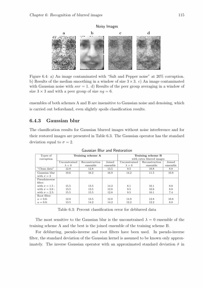
Chapter 6: Recognition of blurred images 115
Noisy Images
a b c d
Figure 6.4: a) An image contaminated with “Salt and Pepper noise” at 20% corruption.b) Results of the median smoothing in a window of size 3× 3. c) An image contaminatedwith Gaussian noise with snr = 1. d) Results of the peer group averaging in a window ofsize 3× 3 and with a peer group of size ng = 6.
ensembles of both schemes A and B are insensitive to Gaussian noise and denoising, which
is carried out beforehand, even slightly spoils classification results.
6.4.3 Gaussian blur
The classification results for Gaussian blurred images without noise interference and for
their restored images are presented in Table 6.3. The Gaussian operator has the standard
deviation equal to σ = 2.
Gaussian Blur and RestorationTypes of Training scheme A Training scheme B
corruption with extra blurred imagesUnconstrained Reconstruction Joined Unconstrained Reconstruction Joined
λ = 0 ensemble ensemble λ = 0 ensemble ensemble”Clean data” 12.8 12.8 13.5 9.5 10.8 8.8
Gaussian blur 19.6 16.2 16.9 14.2 11.5 10.8with σ = 2Pseudoinversefilter:with σ = 1.5 : 15.5 13.5 14.2 8.1 10.1 8.8with σ = 2.0 : 13.5 13.5 12.8 9.5 10.8 8.8with σ = 2.5: 15.5 15.5 12.8 9.5 10.1 7.4Root filter:α = 0.6: 12.8 13.5 12.8 14.9 12.8 10.8α = 0.8: 13.5 14.2 14.2 12.2 12.2 8.8
Table 6.3: Percent classification error for deblurred data
The most sensitive to the Gaussian blur is the unconstrained λ = 0 ensemble of the
training scheme A and the best is the joined ensemble of the training scheme B.
For deblurring, pseudo-inverse and root filters have been used. In pseudo-inverse
filter, the standard deviation of the Gaussian kernel is assumed to be known only approx-
imately. The inverse Gaussian operator with an approximated standard deviation σ in
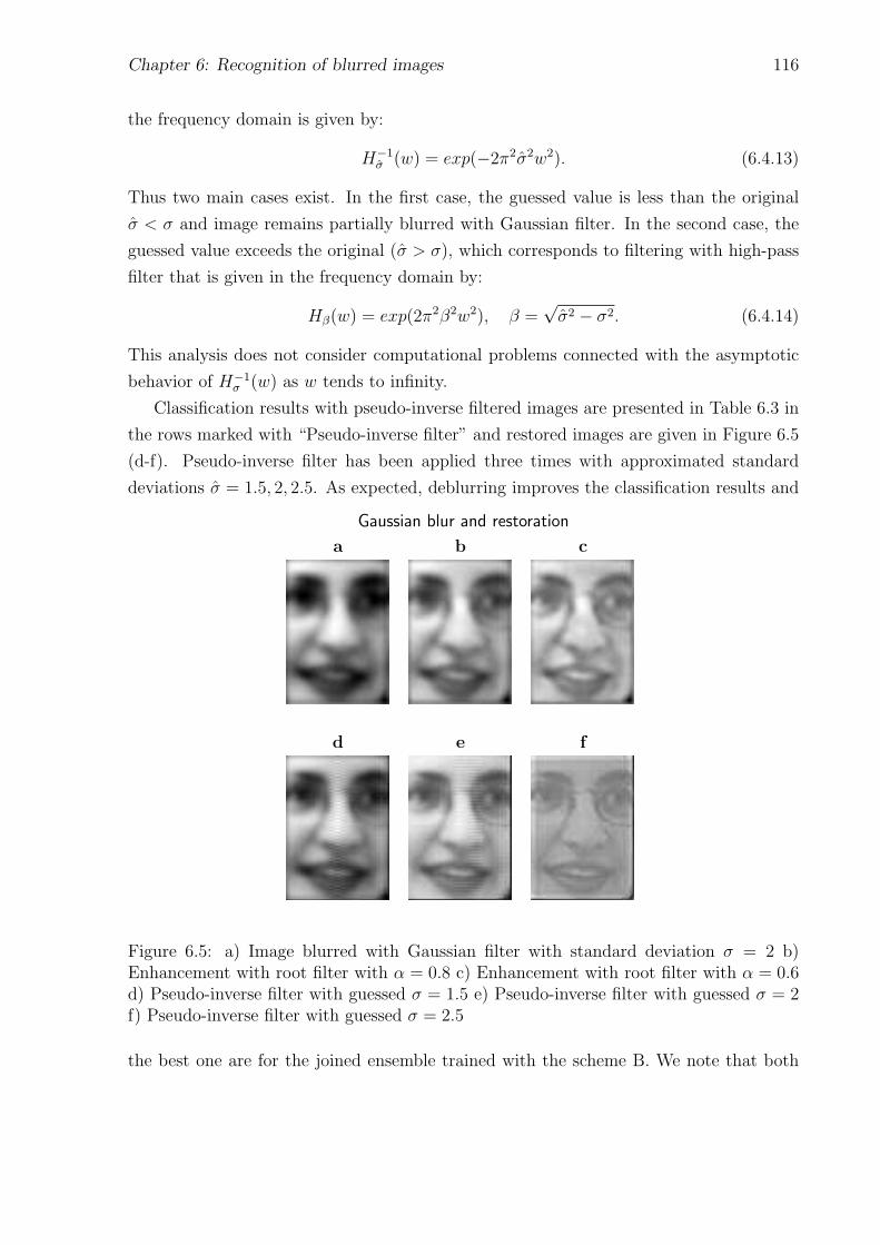
Chapter 6: Recognition of blurred images 116
the frequency domain is given by:
H−1σ (w) = exp(−2π2σ2w2). (6.4.13)
Thus two main cases exist. In the first case, the guessed value is less than the original
σ < σ and image remains partially blurred with Gaussian filter. In the second case, the
guessed value exceeds the original (σ > σ), which corresponds to filtering with high-pass
filter that is given in the frequency domain by:
Hβ(w) = exp(2π2β2w2), β =√σ2 − σ2. (6.4.14)
This analysis does not consider computational problems connected with the asymptotic
behavior of H−1σ (w) as w tends to infinity.
Classification results with pseudo-inverse filtered images are presented in Table 6.3 in
the rows marked with “Pseudo-inverse filter” and restored images are given in Figure 6.5
(d-f). Pseudo-inverse filter has been applied three times with approximated standard
deviations σ = 1.5, 2, 2.5. As expected, deblurring improves the classification results and
Gaussian blur and restoration
a b c
d e f
Figure 6.5: a) Image blurred with Gaussian filter with standard deviation σ = 2 b)Enhancement with root filter with α = 0.8 c) Enhancement with root filter with α = 0.6d) Pseudo-inverse filter with guessed σ = 1.5 e) Pseudo-inverse filter with guessed σ = 2f) Pseudo-inverse filter with guessed σ = 2.5
the best one are for the joined ensemble trained with the scheme B. We note that both
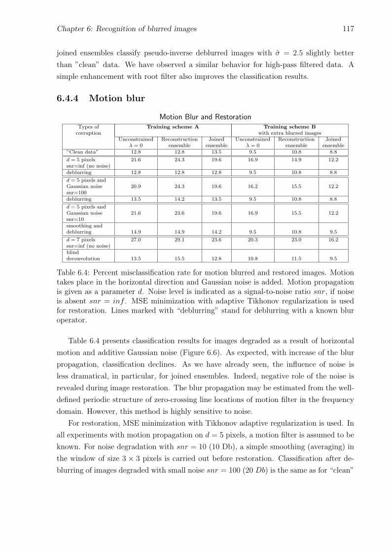
Chapter 6: Recognition of blurred images 117
joined ensembles classify pseudo-inverse deblurred images with σ = 2.5 slightly better
than ”clean” data. We have observed a similar behavior for high-pass filtered data. A
simple enhancement with root filter also improves the classification results.
6.4.4 Motion blur
Motion Blur and RestorationTypes of Training scheme A Training scheme B
corruption with extra blurred imagesUnconstrained Reconstruction Joined Unconstrained Reconstruction Joined
λ = 0 ensemble ensemble λ = 0 ensemble ensemble”Clean data” 12.8 12.8 13.5 9.5 10.8 8.8
d = 5 pixels 21.6 24.3 19.6 16.9 14.9 12.2snr=inf (no noise)deblurring 12.8 12.8 12.8 9.5 10.8 8.8
d = 5 pixels andGaussian noise 20.9 24.3 19.6 16.2 15.5 12.2snr=100deblurring 13.5 14.2 13.5 9.5 10.8 8.8
d = 5 pixels andGaussian noise 21.6 23.6 19.6 16.9 15.5 12.2snr=10smoothing anddeblurring 14.9 14.9 14.2 9.5 10.8 9.5
d = 7 pixels 27.0 29.1 23.6 20.3 23.0 16.2snr=inf (no noise)blinddeconvolution 13.5 15.5 12.8 10.8 11.5 9.5
Table 6.4: Percent misclassification rate for motion blurred and restored images. Motiontakes place in the horizontal direction and Gaussian noise is added. Motion propagationis given as a parameter d. Noise level is indicated as a signal-to-noise ratio snr, if noiseis absent snr = inf . MSE minimization with adaptive Tikhonov regularization is usedfor restoration. Lines marked with “deblurring” stand for deblurring with a known bluroperator.
Table 6.4 presents classification results for images degraded as a result of horizontal
motion and additive Gaussian noise (Figure 6.6). As expected, with increase of the blur
propagation, classification declines. As we have already seen, the influence of noise is
less dramatical, in particular, for joined ensembles. Indeed, negative role of the noise is
revealed during image restoration. The blur propagation may be estimated from the well-
defined periodic structure of zero-crossing line locations of motion filter in the frequency
domain. However, this method is highly sensitive to noise.
For restoration, MSE minimization with Tikhonov adaptive regularization is used. In
all experiments with motion propagation on d = 5 pixels, a motion filter is assumed to be
known. For noise degradation with snr = 10 (10 Db), a simple smoothing (averaging) in
the window of size 3 × 3 pixels is carried out before restoration. Classification after de-
blurring of images degraded with small noise snr = 100 (20 Db) is the same as for “clean”
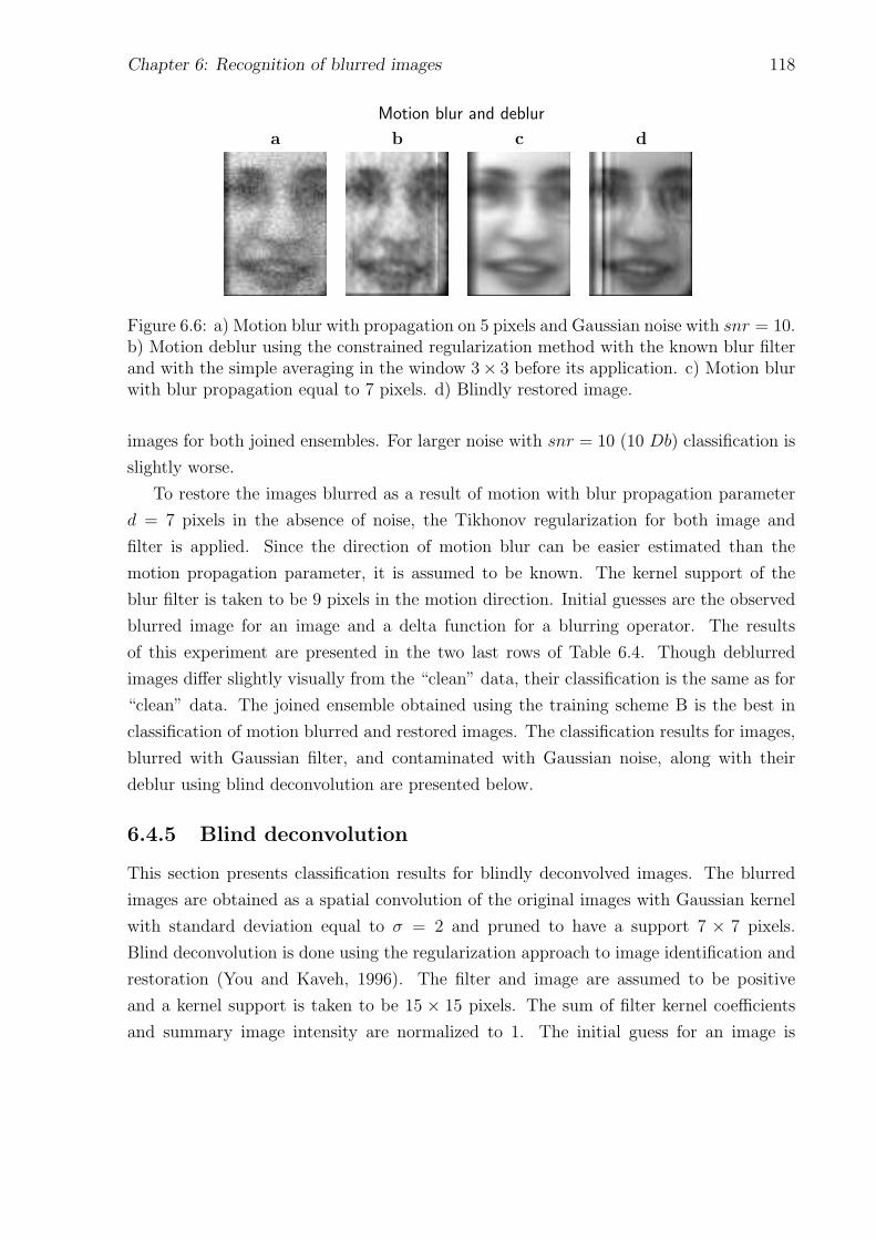
Chapter 6: Recognition of blurred images 118
Motion blur and deblur
a b c d
Figure 6.6: a) Motion blur with propagation on 5 pixels and Gaussian noise with snr = 10.b) Motion deblur using the constrained regularization method with the known blur filterand with the simple averaging in the window 3× 3 before its application. c) Motion blurwith blur propagation equal to 7 pixels. d) Blindly restored image.
images for both joined ensembles. For larger noise with snr = 10 (10 Db) classification is
slightly worse.
To restore the images blurred as a result of motion with blur propagation parameter
d = 7 pixels in the absence of noise, the Tikhonov regularization for both image and
filter is applied. Since the direction of motion blur can be easier estimated than the
motion propagation parameter, it is assumed to be known. The kernel support of the
blur filter is taken to be 9 pixels in the motion direction. Initial guesses are the observed
blurred image for an image and a delta function for a blurring operator. The results
of this experiment are presented in the two last rows of Table 6.4. Though deblurred
images differ slightly visually from the “clean” data, their classification is the same as for
“clean” data. The joined ensemble obtained using the training scheme B is the best in
classification of motion blurred and restored images. The classification results for images,
blurred with Gaussian filter, and contaminated with Gaussian noise, along with their
deblur using blind deconvolution are presented below.
6.4.5 Blind deconvolution
This section presents classification results for blindly deconvolved images. The blurred
images are obtained as a spatial convolution of the original images with Gaussian kernel
with standard deviation equal to σ = 2 and pruned to have a support 7 × 7 pixels.
Blind deconvolution is done using the regularization approach to image identification and
restoration (You and Kaveh, 1996). The filter and image are assumed to be positive
and a kernel support is taken to be 15 × 15 pixels. The sum of filter kernel coefficients
and summary image intensity are normalized to 1. The initial guess for an image is

Chapter 6: Recognition of blurred images 119
the degraded face and we start from a delta function filter, no symmetry constraints
(Chan and Wong, 1997) are used. The regularization parameters are set by hand from
visual appearance once and for all images. An image blurred, with a truncated Gaussian
filter, and contaminated with Gaussian noise of snr = 100, and its blind deconvolution
are presented in Figure 6.7. Classification results for two cases, with and without noise
Blind deconvolution
a b c d
Figure 6.7: a) Image blurred with Gaussian filter with standard deviation σ = 2, prunedto a support area 7 × 7 and Gaussian noise with snr = 100. b) Blind deblurring of thedegraded image. c) Original filter. d) Found filter, pruned to the same support as theoriginal filter.
interference, are presented in Table 6.5.
Blind DeconvolutionTypes of Training scheme A Training scheme B
corruption with extra blurred imagesUnconstrained Reconstruction Joined Unconstrained Reconstruction Joined
λ = 0 ensemble ensemble λ = 0 ensemble ensemble”Clean data” 12.8 12.8 13.5 9.5 10.8 8.8
Blur with pruned 18.2 16.2 17.6 10.1 10.1 10.8Gaussian filterBlinddeconvolution 12.8 13.5 12.8 9.5 10.8 8.1
Blur with prunedGaussian filterand Gaussian 18.9 16.2 18.2 10.8 10.1 10.8noise, snr = 100Blinddeconvolution 12.8 14.2 12.8 10.1 10.1 8.8
Table 6.5: Percent misclassification rate for blurred and blindly deblurred images. Theimages are blurred with pruned Gaussian filter.
We note that between ensembles obtained with the training scheme A, reconstruction
ensemble is the less sensitive to blurring and noise. Ensembles obtained with the training
scheme B are less sensitive to noise and blur. The joined ensemble obtained with the
training scheme B has the best classification performance.

Chapter 6: Recognition of blurred images 120
6.4.6 All training schemes
Recognition of blurred images via schemes A–C
BdB
CdC
AdA
fe
dc
ba
0
10
20
30
Mis
clas
sific
atio
n ra
te %
Figure 6.8: Percent classification error bar graph for reconstructed images. Regressionensembles A-C correspond to joined ensembles obtained using recognition schemes A-C,respectively. Heights of the bars marked with Ad-Cd show misclassification of ensemblesA-C respectively on restored images. See also corresponding Table 6.6 for description ofdegradation types a-f.
Summary classification results for joined ensembles, corresponding to all training
schemes A–C, are presented in Figure 6.8 and Table 6.6. First, we observe that en-
sembles of networks trained using the expanded training data-set are superior to the
joined ensemble trained without blurred images. Secondly, we note that both ensembles
B-C have about the same classification performance and ensemble B is slightly better.
This may be explained by the drastic compression rate, that causes reconstructed images
to look blurred in both cases and results in the similarity of two types of reconstruction
constraints (see Figure 6.9).
The third and important observation is that training with blurred images seems to be
more important than restoration preprocessing. Indeed, recognition of restored images
using scheme A (column and bars marked with Ad) is inferior to degraded image recogni-
tion using schemes B–C. However, as was already marked, usage of image preprocessing
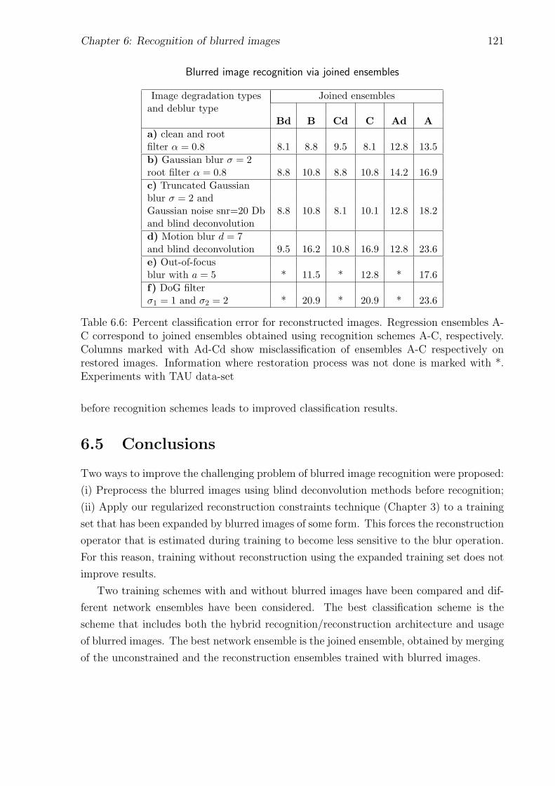
Chapter 6: Recognition of blurred images 121
Blurred image recognition via joined ensembles
Image degradation types Joined ensemblesand deblur type
Bd B Cd C Ad Aa) clean and rootfilter α = 0.8 8.1 8.8 9.5 8.1 12.8 13.5b) Gaussian blur σ = 2root filter α = 0.8 8.8 10.8 8.8 10.8 14.2 16.9c) Truncated Gaussianblur σ = 2 andGaussian noise snr=20 Db 8.8 10.8 8.1 10.1 12.8 18.2and blind deconvolutiond) Motion blur d = 7and blind deconvolution 9.5 16.2 10.8 16.9 12.8 23.6e) Out-of-focusblur with a = 5 * 11.5 * 12.8 * 17.6f) DoG filterσ1 = 1 and σ2 = 2 * 20.9 * 20.9 * 23.6
Table 6.6: Percent classification error for reconstructed images. Regression ensembles A-C correspond to joined ensembles obtained using recognition schemes A-C, respectively.Columns marked with Ad-Cd show misclassification of ensembles A-C respectively onrestored images. Information where restoration process was not done is marked with *.Experiments with TAU data-set
before recognition schemes leads to improved classification results.
6.5 Conclusions
Two ways to improve the challenging problem of blurred image recognition were proposed:
(i) Preprocess the blurred images using blind deconvolution methods before recognition;
(ii) Apply our regularized reconstruction constraints technique (Chapter 3) to a training
set that has been expanded by blurred images of some form. This forces the reconstruction
operator that is estimated during training to become less sensitive to the blur operation.
For this reason, training without reconstruction using the expanded training set does not
improve results.
Two training schemes with and without blurred images have been compared and dif-
ferent network ensembles have been considered. The best classification scheme is the
scheme that includes both the hybrid recognition/reconstruction architecture and usage
of blurred images. The best network ensemble is the joined ensemble, obtained by merging
of the unconstrained and the reconstruction ensembles trained with blurred images.

Chapter 6: Recognition of blurred images 122
We have shown that the combination of both ways, the restoration and regularized
classification approach are superior to each one separately. Since restoration techniques
are very sensitive to noise and require a priori knowledge or visual human interaction, it is
important that the hybrid classification/reconstruction is less sensitive to the restoration
parameters.

Chapter 6: Recognition of blurred images 123
Reconstruction of Gaussian blurred images
Training scheme B
Training scheme C
Figure 6.9: Reconstruction of Gaussian blurred images by Neural Networks obtained usingtraining schemes B–C. Images in the top row from left to right are an original image, its“caricature” image and Gaussian blurred image. In the middle row, images reconstructedby Neural Networks with λ = 0.05, 0.15, 0.25 and with reconstruction defined by thetraining scheme B are presented. In the bottom row, images reconstructed by NeuralNetworks with λ = 0.05, 0.15, 0.25 and with reconstruction defined by the training schemeC are presented. Note that though images in the middle row are sharper than images inthe bottom row, they nevertheless look blurred.

Chapter 7
Summary and future work
In this final chapter, we summarize the main contribution of the thesis and present several
possible directions for future work.
7.1 Summary
Our primary goal in this thesis was to improve the performance of a high dimensional
image recognition task, by extracting a good hidden representation of the image data.
We developed several approaches to achieve a good generalization in image recognition.
First we developed a novel hybrid feed-forward reconstruction/recognition network
architecture, with two output sublayers for reconstruction and recognition, and one com-
mon hidden layer shared by both tasks (Chapter 3). The network was trained to minimize
concurrently MSE of reconstruction and recognition output sublayers.
Though, a similar architecture was used previously (see Section 3.1.5), we first used
it for improving image recognition and gave a new interpretation of the hybrid network
as a tool to control bias via imposing a novel type of reconstruction bias constraints. In
addition, we introduced a trade-off parameter λ that defines the influence of each of the
tasks and is unknown a-priori. We have considered networks with different values of λ,
instead of considering only a single value, as has been proposed previously.
In addition, the network and its learning rule were interpreted in the MDL and
Bayesian frameworks. In Bayesian formulation, the network is trained to maximize the
conditional joint probability of the reconstructed image and its class label given the ob-
served image. In the proposed architecture, the reconstructed image and its class label
are independent given the observed image and under the assumption of a Gaussian distri-
bution of the errors, this maximization leads to the proposed learning rule. The trade-off
parameter λ emerges as a hyper-parameter and according to the Bayesian theory, the
right approach is to integrate predictors over this parameter. If the initial weights of the
124

Chapter 7: Summary and future work 125
feed-forward network are also considered as hyper-parameters, then the predictor f is
given by:
f(x) =∫ ∫
fλ,w0(x)p(λ,w0|X )dw0dλ (7.1.1)
This interpretation has led us to the second approach to improve image recognition.
We have proposed to replace the integration in Eq. 7.1.1 by a rough approximation via
ensemble network averaging. Networks with a good recognition performance were included
in the ensemble and their posterior probabilities p(λ,w0|X ) were assumed to be equal.
It is well known, that ensemble averaging can reduce the variance portion of the
prediction error. We have considered three ensemble types (Chapter 5):
• Unconstrained ensemble, which corresponds to integration over w0 for λ = 0
• Reconstruction ensemble, which corresponds to integration over λ for fixed w0
• Joined ensemble, which is a combination of unconstrained and reconstruction en-
sembles and corresponds to integration over both parameters
We have shown that the joined ensemble is superior to the reconstruction ensemble, which
in turn is superior to the unconstrained ensemble, in recognition of images degraded by
Gaussian and pulse noises as well as by partial occlusion or image blur.
Our third contribution concerns especially in improving recognition of blurred images.
It is well known, that in many practical recognition tasks, images appear blurred due to
motion, bad weather conditions and defocusing of cameras. Three ways were proposed
for improving blurred image recognition:
1. Expanding the training set with Gaussian blurred images
2. During training, constraining reconstruction of the blurred images to the original
clean images
3. Application of state of the art restoration methods to the blurred images before
using the hybrid architecture
The first two ways have led to two additional joined ensembles that we trained with extra
Gaussian images and reconstruction constraints. Reconstruction was either to the blurred
image or the clean (non-blurred) image (Chapter 6). We have shown that ensembles that
were trained on extra (blurred) images had improved recognition performance on different
image degradation types. In addition, we have shown that training with extra images

Chapter 7: Summary and future work 126
combined with restoration techniques achieved robust and best recognition performance
under a wide range of blur operators and parameters.
Additional contribution of the thesis is developing hybrid networks with unsupervised
learning constraints (Chapter 5), which were mainly used for comparison with reconstruc-
tion constraints. We have shown that these constraints can also be used for improving
the recognition performance instead, or in parallel with reconstruction constraints.
In addition, we addressed the issue of a network interpretability by investigating the
network hidden representation and hidden weights (Appendix 5.7), and by the saliency
map construction (Section 5.5). In contrast, to explicit understanding what information
is encoded in the hidden space, the saliency map allows one to decide which features in the
input are more important. We showed that usage of the saliency maps further improves
recognition of images degraded with “Salt and Pepper” noise.
7.2 Directions for future work
Non face data sets We have tested the proposed hybrid system on facial data sets.
Faces, however, are a special type of stimuli where all pixels are important (Biederman and
Kalocsai, 1997). It should be interesting to test the hybrid architecture performance on
data sets of similar objects, such as military images (different kinds of tanks, ships, cars,
etc.), medical images (different kinds of tumor cells) and astronomical images (images of
different stars and galaxies).
Ensemble interpretation In Appendix 5.7, hidden representations of single Neural
Networks with reconstruction constraints were investigated. In addition it was noted,
that network ensemble hidden representation is not well defined. However, another form
of interpretation using the mean derivative (over networks and images) with respect to
the inputs for each of the classes (Intrator and Intrator, 1993) may be very interesting.
Recurrent network architecture Images reconstructed by Neural Networks (which
we called prototypes, see Section 5.5) are reduced representation of the original images,
since a drastic compression occurs via the bottleneck architecture (see Figure 5.5). How-
ever, as can be seen, prototypes corresponding to the same class look similar, while
prototypes corresponding to different classes look different. It is also clear that a good
reconstruction/recognition network has to be able to recognize its own prototype images.
Table 7.1 presents recognition performance of the unconstrained and reconstruction en-
sembles (see Chapter 3), when they are tested on the prototype images. These results

Chapter 7: Summary and future work 127
Classification error for reconstructed images
Types of degradation Regression EnsemblesUnconstrained Reconstruction A Reconstruction B
”Clean data”input 0.5 1.5 1prototype 1.5 2.1 2.6“Salt and Pepper”noise with d = 0.2input 7.2 12.8 13.3prototype 7.2 11.8 12.8“nose” occlusioninput 0.5 1.5 1.5prototype 1.5 2.1 2.1“half face”occlusioninput 5.6 5.6 6.2prototype 6.2 6.7 7.2”DOG 1-2”input 7.7 4.1 8.2prototype 8.2 4.1 8.2
Table 7.1: Errors are given in percent (Pentland data-set).
show that networks are better in recognition of the original images than their own pro-
totypes. This can be corrected by propagating reconstructed images back to the input
layer during learning. In other words, during learning we propose to extend the training
set with extra images xe, which are a linear combination of the input x and its prototype
image xp:
xe = ρ(t)x+ (1− ρ(t))xp, ρ ∈ [0, 1],
where ρ(t) is a non increasing function of the training epoch number t, equal to 1 at the
beginning and 0 at the infinity. This procedure may give better results that should be
tested by simulation.
Network ensembles We considered ensembles corresponding to the simplest version
of integration (7.1.1) with equal posterior probability p(λ,w0|X ). Though it is impossible
to find posterior probability p(λ,w0|X ) analytically, it may be heuristically postulated.
Therefore, integration (7.1.1) may be replaced by the weighted network ensemble aver-
aging. We tried to use weights based on different error types between input and output
reconstruction layers, such as Euclidean metric or correlation measure and their soft ver-
sion using the exp(−x) function. However, our preliminary experiments do not show
significant recognition improvement.
Since the hybrid networks solve both recognition and reconstruction tasks, it is reason-
able to use the ensemble of hybrid networks for reconstruction. The obtained prototype
may be used for recognition by all the networks.
Chapter 7: Summary and future work 128
Degradation invariance constraints We considered the simplest version of invari-
ance constraints expanding the data with Gaussian blurred images. Another type of
invariance constraints is the tangent prop constraint, that was used for a group of geo-
metrical transformations (see Section 2.3.2). This type of constraints may be adapted for
different types of blur operations for both recognition and reconstruction tasks.
Generalization It would be interesting to generalize the hybrid architecture in the di-
rection taken by other generative models (Hinton and Ghahramani, 1997; Ullman, 1995).

Bibliography
Abu-Mostafa, Y. (1993). A method for learning from hints. In Touretzky, D. S. and Lipp-
mann, R. P., editors, Advances in Neural Information Processing Systems, volume 5,
pages 73–80. Morgan Kaufmann, San Mateo, CA.
Abu-Mostafa, Y. (1994). Learning from hints. J. of Complexity, 10:165–178.
Amari, S., Cichocki, A., and Yang, H. H. (1996). A new learning algorithm for blind
signal separation. In Tesauro, G., Touretzky, D., and Leen, T., editors, Advances in
Neural Information Processing Systems, volume 8, pages 757–763. MIT Press.
Atick, J. (1992). Entropy minimization: A design principle for sensory perception. In-
ternational Journal of Neural Systems. Proceedings of the Neural Networks: From
biology to High Energy Physics, 3:81–90.
Atick, J. J., Griffin, P. A., and Redlich, A. N. (1995). Face recognition from live video for
real-world applications. Advanced Imaging.
Atick, J. J. and Redlich, N. (1992). What does the retina know about natural scenes.
Neural Computation, 4:196–210.
Baird, H. (1990). Document image defect models. In IAPR, Workshop on Syntatic and
Structural Pattern Recognition, pages 38–46. Murray Hill, NJ.
Baluja, S. (1996). Expectation-based selective attention. PhD thesis, School of computer
science, CMU.
Baluja, S. and Pomerleau, D. A. (1995). Using the representation in a neural network’s
hidden layer for task-specific focus of attention. In Proceedings of the International
Joint Conference on Artificial Intelligence, Montreal, Canada.
Barlow, H. B. (1961). Possible principles underlying the transfomations of sensory mes-
sages. In Rosenblith, W., editor, Sensory Communication, pages 217–234. MIT Press,
Cambridge, MA.
129
Bibliography 130
Barlow, H. B. (1989). Unsupervised learning. Neural Computation, 1(3):295–311.
Baron, R. J. (1981). Mechanisms of human facial recognition. The international Journal
of Robotics research, 15:137–178.
Bartlett, Stewart, M., Lades, Martin, H., and Sejnowski (1998). Independent component
representations for face recognition. Proceedings of the SPIE Symposium on Elec-
tronic Imaging: Science and Technology. Conference on Human Vision and Elec-
tronic Imaging III.
Bell, A. J. and Sejnowski, T. J. (1995). An information-maximisation approach to blind
separation and blind deconvolution. Neural Computation, 7(6):1129–1159.
Bellman, R. E. (1961). Adaptive Control Processes. Princeton University Press, Princeton,
NJ.
Bhanu, B. and Ming, J. C. (1987). Recognition of occluded objects: A cluster-structure
algorithm. Pattern Recognition, 20(2):199–211.
Biederman, I. and Kalocsai, P. (1997). Neurocomputational bases of object and face
recognition. Philosophical Transactions of the Royal Society of London B, 352:1203–
1219. Comparison of face and other object recognition.
Bienenstock, E. L., Cooper, L. N., and Munro, P. W. (1982). Theory for the development
of neuron selectivity: orientation specificity and binocular interaction in visual cortex.
Journal Neuroscience, 2:32–48.
Bishop, C. M. (1995a). Neural Networks for Pattern Recognition. Oxford University Press.
Bishop, C. M. (1995b). Training with noise is equivalent to Tikhonov regularization.
Neural Computation, 7(1):108–116.
Blais, B. S., Intrator, N., Shouval, H., and Cooper, L. N. (1998). Receptive field forma-
tion in natural scene environments: comparison of single cell learning rules. Neural
Computation, 10(7):1797–1813.
Bourlard, H. and Kamp, Y. (1988). Auto-association by multilayer perceptrons and
singular value decomposition. Biological Cybernetics, 59:291–294.
Brunelli, R. and Poggio, T. (1992). Face recognition through geometrical features. Pro-
ceedings of the 2nd European Conference on Computer Vision.

Bibliography 131
Brunelli, R. and Poggio, T. (1993). Face recognition: Features versus templates. IEEE
PAMI, 15:1042–1052.
Cannon, M. (1976). Blind deconvolution of spatially invariant image blurs with phase.
icassp, 24:58–63.
Caruana, R. (1995). Learning many related tasks at the same time with backpropagation.
In Tesauro, G., Touretzky, D., and Leen, T., editors, Advances in Neural Information
Processing Systems, volume 7, pages 657–664. Morgan Kaufmann, San Mateo, CA.
Chan, T. F. and Wong, C. K. (1997). Total variation blind deconvolution. Technical
report, UCLA.
Chellapa, Wilson, and Sirohey (1995). Human and machine face recognition of faces.
Proceedings of the IEEE, pages 704–740.
Chopper (1997). Autonomous helicopter project. CMU.
Coifman, R. R. and Wickerhauser, M. (1992). Entropy-based algorithms for best basis
selection. IEEE Trans. Info. Theory, 38(2):713–719.
Comon, P. (1994). Independent component analysis, a new concept? Signal Processing,
36:287–314.
Connolly (1997). Robotics internet resources page. UMass Laboratory for Perceptual
Robotics.
Cotrrell, G. W. and Fleming, M. K. (1990). Categorization of faces using unsupervised
feature extraction. Proc. Int. Conf. on Neural Networks, 2:65–70.
Cottrell, Munro, P., and Zipser., D. (1987). Image compression by back propagation: An
example of extensional programming. Advances in Cognitive science, 3.
Cover, T. M. and Thomas, J. A. (1991). Elements of Information Theory. Wiley-
Interscience, New York.
Dempster, A. P., Laird, N. M., and Rubin, D. B. (1977). Maximum likelihood from
incomplete data via the EM algorithm. Proceedings of the Royal Statistical Society,
B-39:1–38.
Duda, R. O. and Hart, P. E. (1973). Pattern Classification and Scene Analysis. John
Wiley, New York.

Bibliography 132
Edelman, S., Reisfeld, D., and Yeshurun, Y. (1992). Learning to recognize faces from
examples. In Proceedings of the 2nd European Conference on Computer Vision, pages
787–791, Santa Margherita Ligure, Italy.
Efron, B. and Tibshirani, R. (1993). An Introduction to the Bootstrap. Chapman and
Hall, New York.
Elman, J. L. and Zipser, D. (1988). Learning the hidden structure of speech. Journal of
the Acoustical Society of America, 4(83):1615–1626.
Fabian, R. and Malah, D. (1991). Robust identification of motion and out-of-focus blur
parameters from blurred and noisy images. cvgip, 53(5):403–412.
Field, D. J. (1994). What is the goal of sensory coding. Neural Computation, 6:559–601.
Friedman, J. H. (1987). Exploratory projection pursuit. Journal of the American Statis-
tical Association, 82:249–266.
Fukunaga, K. (1990). Introduction to Statistical Pattern Recognition. Academic press,
London.
Geman, S., Bienenstock, E., and Doursat, R. (1992). Neural networks and the bias-
variance dilemma. Neural Computation, 4:1–58.
Girolami, M. and Fyfe, C. (1996). Negentropy and kurtosis as projection pursuit indices
provide generalised ica algorithms. Preprint.
Gluck, M. A. and Myers, C. E. (1993). Hippocampal mediation of stimulus representation:
A computational theory. Hippocampus, 3(4):491–516.
Gonzalez, R. C. and Wintz, P. (1993). Digital Image Processing. Addison-Wesley Pub-
lishing Company.
Grenander, U. (1978). Pattern analysis. Springer-Verlag, New York.
Gutta, S., Huang, J., Imam, I. F., and Wechsler, H. (1996). Face and hand gesture
recognition using hybrid classifiers. In Proceedings of the second IEEE International
Conference on Automatic Face and Gesture Recognition, pages 164–169, Washington,
Brussels, Tokyo.
Hancock, J. B., Baddeley, R. J., and Smith, L. S. (1992). The principal components of
natural images. In Network: Computation in Neural Systems, 3(1):61–70.

Bibliography 133
Hansen, L. K. and Salamon, P. (1990). Neural network ensembles. IEEE Transactions
on Pattern Analysis and Machine Intellignce, 12(10):993–1001.
Haykin, S. (1994). Neural Networks. Imprint MACMILLAN, New York.
Hertz, J., Krogh, A., and Palmer, R. G. (1991). Introduction to the Theory of Neural
Computation. Addison Welsley, New York.
Hinton, G. E., Dayan, P., Frey, B. J., and Neal, R. M. (1995). The ”Wake-Sleep” algorithm
for unsupervised neural networks. Science, 268:1158–1161.
Hinton, G. E. and Ghahramani, Z. (1997). Generative models for discovering sparse
distributed representations. Philosophical Transactions of the Royal Society B,
352:1177–1190.
Hinton, G. E. and Zemel, R. S. (1994). Autoencoders, minimum description length, and
helmholtz free energy. Advances in Neural Information Processing Systems.
Hirukawa (1997). Etl robotics research group. Japan.
Hochberg, J. (1974). Organization and the gestalt tradition. In Carterette, C. and Fried-
man, M., editors, Handbook of Perception, New York. Academic Press.
Hochreiter, S. and Schmidhuber, J. (1997). Flat minima. Neural Computation, 9(1):1–42.
Howell, A. J. (1997). Automatic Face Recognition using Radial Basis Function Networks.
PhD thesis, University of Sussex.
Huber, P. J. (1985). Projection pursuit. (with discussion). The Annals of Statistics,
13:435–475.
Humel, R. A., Kimia, B. B., and Zucker, S. W. (1987). Deblurring Gaussian blur. cvgip,
38(1):66–80.
Hyvarinen (1997a). Independent component analysis by minimization of mutual infor-
mation. Technical report a46, Laboratory of Computer and Information Science,
Helsinki University of Technology.
Hyvarinen (1997b). New approximations of differential entropy for independent compo-
nent analysis and projection pursuit. Technical report a46, Laboratory of Computer
and Information Science, Helsinki University of Technology.
Bibliography 134
Intrator, N. (1993a). Combining exploratory projection pursuit and projection pursuit
regression with application to neural networks. Neural Computation, 5(3):443–455.
Intrator, N. (1993b). On the combination of supervised and unsupervised learning. Physica
A, pages 655–661.
Intrator, N. (1999). Robust prediction in many parameter models: Specific control of
variance and bias. In Kay, J. W. and Titterington, D. M., editors, Statistics and
Neural Networks: Advances at the Interface. Oxford University Press. To appear.
Intrator, N. and Cooper, L. N. (1992). Objective function formulation of the BCM the-
ory of visual cortical plasticity: Statistical connections, stability conditions. Neural
Networks, 5:3–17.
Intrator, N. and Cooper, L. N. (1995). BCM theory of visual cortical plasticity. In Arbib,
M., editor, The Handbook of Brain Theory and Neural Networks, pages 153–157. MIT
Press.
Intrator, N. and Edelman, S. (1996). Making a low-dimensional representation suitable
for diverse tasks. Connection Science, Special issue on Reuse of Neural Networks
Through Transfer, 8(2):205–224. Also in Learning to Learn, S. Thrun and L. Pratt
(ed., Kluwer press.).
Intrator, N., Reisfeld, D., and Yeshurun, Y. (1996). Face recognition using a hybrid
supervised/unsupervised neural network. Pattern Recognition Letters, 17:67–76.
Intrator, O. and Intrator, N. (1993). Interpreting neural-network models. Preprint.
Jacobs, R. (1997). Bias/variance analyses of mixtures-o-experts architectures. Neural
Computation, pages 369–383.
Jain, A., Zheng, Y., and Lakshmanan, S. (1996). Object matching using deformable
templates. T-PAMI, 18:267–278.
Jain, A. K. (1989). Fundamentals of Digital Image Processing. Prentice Hall, London.
Japkowicz, N., Myers, C., and Cluck, M. (1995). A novelty detection approach to clas-
sification. In the proceedings of the Fourteenth International Joint Conference on
Artificial Intelligence, pages 518–523.
Jordan, M., editor (1999). Learning in Graphical Models. The MIT Press, Cambridge,
Massachusetts, London, England.

Bibliography 135
Kandel, E. R. and Schwartz, J. H. (1991). Principles of Neural Science. Elsevier, New
York, third edition.
Kanizsa and Gaetano (1970). Organization in Vision: Essays on Gestalt Perception.
Praeger, New York.
Katsaggelos, A. K. (1989). Iterative image restoration algorithms. Optical Engineering,
28(7):735–748.
Kimia, B. B. and Zucker, S. W. (1993). Analytic inverse of discrete Gaussian blur. Optical
Engineering, 32(1):166–176.
Kirby, M. and Sirovich, L. (1990). Application of the Karhunen-Loeve procedure for
characterization of human faces. PAMI, 12(1):103–108.
Kohavi, R. (1995). A study of cross-validation and bootstrap for accuracy estimation and
model selection. International Joint Conference on Artificial Intelligence.
Kramer, M. A. (1991). Nonlinear principal component analysis using autoassociative
neural networks. AIChe Journal, 37(2):233–243.
Kung, S. Y. and Diamantaras, C. I. (1990). A neural network learning algorithm for adap-
tive principal component extraction (apex). International Conference on Acoustics,
Speech and Signal Processing, 2:861–864.
Lai, K. F. (1994). Deformable Contours: Modeling, Extraction , Detection and Classifica-
tion, Phd Thesis. PhD thesis, University of Wisconsin-Madison,Electrical Engineer-
ing.
Lee, T., Girolami, M., Bell, A. J., and Sejnowski, T. J. (1998). A unifying information-
theoretic framework for independent component analysis. International Journal on
Mathematical and Computer Modeling. in press.
Leen, T. (1995). From data distribution to regularization in invariant learning. In Touret-
zky, D. S. and Lippmann, R. P., editors, Advances in Neural Information Processing
Systems, volume 7, pages 223–230. Morgan Kaufmann, San Mateo, CA.
Lesher, G. W. (1995). Illusory contours: Toward a neurally based perceptual theory.
Psychonomic Bulletin abd Review, 2(3).
Linsker, R. (1988). Self-organization in a perceptual network. IEEE. Computer, 88:105–
117.
Bibliography 136
Liu, H.-C. and Srinath, M. D. (1984). Partial shape classification using contour matching
in distance transformation. IEEE Transactions on PAMI, 12(11):1072–1078.
Luenberger, D. G. (1989). Linear and nonlinear programming. ADDISON-WESLEY,
READING, MASS. second edition.
MacKay, D. (1992). Bayesian intertpolation. Neural Computation, 4(3):415–447.
MacKay, D. (1996). Maximum likelihood and covariant algorithms for independent com-
ponent analysis. Technical report draft 3.7, Cavendish laboratory, University of Cam-
bridge.
Marr, D. (1982). Vision. Imprint FREEMAN, New York.
Meir, R. (1994). Bias, variance and the combination of estimators: The case of linear least
squares. ftp://archive.cis.ohio-state.edu/pub/neuroprose/meir.bias-variance.ps.Z.
Miller, K. D. (1995). Receptive fields and maps in the visual cortex: Models of ocular
dominance and orientation columns. In Domany, E., van Hemmen, J. L., and Schul-
ten, K., editors, Models of Neural Networks 3, pages 55–78. Springer-Verlag, New
York.
Moghaddam, B. and Pentland., A. (1994). Face recognition using view-based and mod-
ular eigenspaces. Automatic Systems for the identification and Inspection of Hu-
mans,SPIE, 2227.
Moses, Y. (1994). Face recognition: the problem of compensating for illumination changes.
IEEE Transactions on Pattern Analysis and Machine Intelligence, 19(7):721–732.
Mougeot, M., Azencott, R., and Angeniol, B. (1991). Image compression with back
propagation: Improvement of the visual restoration using different cost functions.
Neural Networks, 4:467–476.
Munro, P. (1997). Noisy encoders. NIPS*97 Workshop: Advances in Autoencoder-
Autoassociator Based Computations.
Murase, H. and Nayar, S. K. (1993). Learning object models from appearance. Proceedings
of the Eleventh National Conference on Artificial Intelligence.
Murray, A. F. and Edwards, P. J. (1993). Synaptic weight noise during multilayer per-
ceptron training: Fault tolerance and training improvements. IEEE Transactions on
Neural Networks, 4(4):722–725.

Bibliography 137
Nadal, J.-P. and Parga, N. (1994). Nonlinear neurons in the low-noise limit: a factorial
code maximizes information transfer. Network, 5:565–581.
Naftaly, U., Intrator, N., and Horn, D. (1997). Optimal ensemble averaging of neural
networks. Network, 8(3):283–296.
Neal, R. M. and Hinton, G. E. (1993). A new view of the EM algorithm that justifies
incremental and other variants. Submitted to Biometrica.
Nowlan, S. J. and Hinton, G. E. (1992). Simplifying neural networks by soft weight-
sharing. Neural Computation, 4:473–493.
Oja, E. (1982). A simplified neuron model as a principal component analyzer. Math.
Biology, 15:267–273.
Oja, E. (1995a). The nonlinear pca learning rule and signal separation - mathematical
analysis. Technical Report A26, Helsinki University, CS and Inf. Sci. Lab.
Oja, E. (1995b). Principal and independent components in neural networks - recent
developments. In Proc. VII Italian Workshop on Neural Nets WIRN’95, Vietri sul
Mare, Italy.
Olshausen, B. A. and Field, D. J. (1996). Natural image statistics and efficient coding.
Network, 7:333–339.
O’Toole, A. J., Valentin, D., and Abdi, H. (1991). Categorization and identification of
human face images by neural networks: A review of the linear autoassociative and
principal component approaches. Journal of Biological Systems, 2(3):413–430.
O’Toole, A. J., Valentin, D., and Abdi, H. (1993). A low dimensional representation of
faces in the higher dimensions of the space. Journal of the Optical Society of America,
series A, 10:405–411.
Perrone, M. P. (1993). Improving Regression Estimation: Averaging Methods for Variance
Reduction with Extensions to General Convex Measure Optimization. PhD thesis,
Brown University, Institute for Brain and Neural Systems.
Phillips, P. J. (1998). Support vector machines applied to face recognition. In Touretzky,
D. S. and Lippmann, R. P., editors, Advances in Neural Information Processing
Systems, pages 1–7. Morgan Kaufmann, San Mateo, CA. To appear.

Bibliography 138
Phillips, P. J., Moon, H., Rauss, P. J., and Der, S. Z. (1997). The feret september 1996
database and evaluation procedure. In The First International Conference on Audio
and Video-based Biometric Person Authetication, Crans-Montana, Swizerland.
Phillips, P. J., Rauss, P. J., and Der, S. Z. (1996). Feret (face recognition technology)
recognition algorithm development and test results. Technical report, arl-tr-995, US
Army Research Laboratory Technical Report.
Pomerleau, D. A. (1993). Input reconstruction reliablility estimation. In Giles, C. L.,
Hanson, S. J., and Cowan, J. D., editors, Advances in Neural Information Processing
Systems, volume 5, pages 279–286. Morgan Kaufmann.
Raviv, Y. (1998). Bootstrapping with noise ensemblening. Master’s thesis, The De-
partment of Computer Science. The Raymond and Beverly Sackler Faculty of Exact
Sciences. Tel-Aviv University.
Raviv, Y. and Intrator, N. (1996). Bootstrapping with noise: An effective regularization
technique. Connection Science, Special issue on Combining Estimators, 8:356–372.
Redlich, A. N. (1993). Redundancy reduction as a strategy for unsupervised learning.
Neural Computation, 5:289–304.
Reisfeld, D. (1993). Generalized Symmetry Transforms: Attentional Mechanisms and Face
Recognition. PhD thesis, Tel-Aviv University.
Reisfeld, D., Wolfson, H., and Yeshurun, Y. (1990). Detection of interest points using
symmetry. In Third International Conference on Computer Vision, pages 62–65,
Osaka, Japan.
Rieke, F., Warland, D., de Ruyter van Steveninck, R., and Bialek, W. (1996). Spikes:
Exploring the Neural Code (Computational Neuroscience). The MIT Press, London.
Ripley, B. D. (1996). Pattern Recognition and Neural Networks. Oxford Press.
Rissanen, J. (1985). Minimum description length principle. Encyclopedia of Statistical
Sciences, pages 523–527.
Rosenfeld, A. and Kak, A. C. (1982). Digital Picture Processing. Academic press, New
York.
Roweis, S. (1997). Em algorithms for pca and spca. NIPS97.

Bibliography 139
Roweis, S. and Ghahramani, Z. (1997). A unifying review of linear gaussian models.
Submitted for Publication.
Rudin, L. I., Osher, S., and Fatemi, E. (1992). Nonlinear total variation based noise
removal algorithms. Physica D, 60:259–268.
Samal, A. and Iyengar, P. A. (1992). Automatic recognition and analysis of of human
faces and facial expressions: A survey. Pattern Recognition, 25:65–77.
Samaria, F. and Fallside, F. (1993). Face identification and feature extraction using hidden
markov models. Elsevier.
Sanger, T. D. (1989). Optimal unsupervised learning in a single-layer linear feedforward
neural network. Neural Networks, 2:459–473.
Sato, K., Shah, S., and Aggarwal, J. K. (1998). Partial face recognition using radial basis
function networks. In Proceedings of the third IEEE International Conference on
Automatic Face and Gesture Recognition, pages 288–293, Nara, Japan.
Schwenk, H. and Milgram, M. (1995). Transformation invariant autoassociation with
application to handwritten character recognition. Neural Information Processing
Systems (NIPS 7), pages 991–998.
Sezan, M. I. and Tekalp, A. M. (1990). Survey of recent developments in digital image
restoration. Optical Engineering, 29(5):393–404.
Shannon, C. E. (1948). A mathematical theory of communication. Bell Syst. Tech. J.,
27:379–423 and 623–656.
Simard, P., Victorri, B., LeCun, Y., and Denker, J. (1992). Tangent prop – a formalism
for specifying selected invariances in an adaptive network. In Moody, J., Lippman,
R., and Hanson, S. J., editors, Neural Information Processing Systems, volume 4,
pages 895–903. Morgan Kaufmann, San Mateo, CA.
Stark, H. (1987). Image recovery: Theory and application. Academic press, San Diego.
Stuart, A. and Ord, J. K. (1994). Kendall’s Advanced Theory of Statistics. Edward
Arnold.
Taniguchi, M. and Tresp, V. (1997). Averaging regularized estimators. Neural Computa-
tion, 9:1163–1178.
Bibliography 140
Tankus, A. (1996). Automatic face detection and recognition. Master thesis, Tel-Aviv
University.
Tankus, A., Yeshurun, Y., and Intrator, N. (1997). Face detection by direct convexity
estimation. Pattern Recognition Letters, 18(9):913–922.
Tesauro, G., Touretzky, D., and Leen, T., editors (1995). Neural Network Ensembles,
Cross Validation, and Active Learning. The MIT Press, London.
Tikhonov, A. N. and Arsenin, V. Y. (1977). Solutions of Ill-Posed Problems. V. H.
Winston and Sons, Washington.
Tresp, V. and Taniguchi, M. (1995). Combining estimators using non-constant weighting
function. In Tesauro, G., Touretzky, D., and Leen, T., editors, Advances in Neural
Information Processing Systems, volume 7. MIT Press.
Turk, M. and Pentland, A. (1991). Eigenfaces for recognition. J. of Cognitive Neuro-
science, 3:71–86.
Turk, M. and Pentland, A. (1993). Experiments with eigenfaces. Looking At People
Workshop, IJCAI’93, pages 1–6.
Ullman, S. (1989). Aligning pictoral descriptions: an approach to object recognition.
Cognition, 13:13 – 254.
Ullman, S. (1995). Sequence-seeking and counter-streams: a model for information flow
in the cortex. Cerebral Cortex, 5:1–11.
Valentin, D., Abdi, H., O’Toole, A. J., and Cottrell, G. W. (1994). Connection models of
face processing: A survey. Pattern Recognition, 27:1209–1230.
Vapnik, V. N. (1995). Statistical learning theory. Springer, Check this, New York.
Wahba, G. (1990). Splines Models for Observational Data. Series in Applied Mathematics,
Vol. 59, SIAM, Philadelphia.
Wiskott, L. and von der Malsburg, C. (1993). A neural system for the recognition of
partially occluded objects in cluttered scenes. Int. J. of Pattern Recognition and
Artificial Intelligence, 7(4):935–948. Also in NIPS 7, 1994.
Wiskott, L., von der Malsburg, C., Fellous, and Kruger, N. (1997). Face recognition by
elastic bunch graph matching. IEEE Transactions on Pattern Analysis and Machine
Intelligence, 19(7):775–779.

Bibliography 141
Wolpert, D. H. (1992). Stacked generalization. Neural Networks, 5:241–259.
Yang, H. and Amari, S. (1997). Adaptive on-line learning algorithms for blind separa-
tion – maximum entropy and minimum mutual information. Neural Computation,
9(7):1457–1482.
Yaroslavsky, L. and Eden, M. (1996). Fundamentals of digital optics. Imprint Birkhauser,
Boston.
You, Y.-L. and Kaveh, M. (1996). A regularization approach to joint blur identification
and image restoration. IEEE Transactions on Image Processing, 5(3):416–427.
Yow, K. C. and Cipolla, R. (1996). A probabibilistic framework for perceptual grouping
of features for human face detection. In Proceedings of the second IEEE International
Conference on Automatic Face and Gesture Recognition, pages 16–21, Washington,
Brussels, Tokyo.
Yuille, A. L., Cohen, D., and Hallinan, P. W. (1989). Feature extraction from faces using
defomable tempaltes. In Proc. Computer Vision and Pattern Recognition, pages 104–
109, Washington. IEEE Computer Society Press.
Zemel, R. (1993). A Minimum Description Length Framework for Unsupervised Learning.
PhD thesis, University of Toronto.
Related Documents


