Trade in university training: cross-state variation in the production and stock of college-educated labor

May 9, 2001

Preliminary Comments welcome

Trade in University Training: Cross-State Variation in the Production and Use of College-Educated Labor

John Bound University of Michigan and NBER

Jeffrey Groen

University of Michigan

Gábor Kézdi University of Michigan

Sarah Turner

University of Virginia

Trade in University Training: Cross-State Variation in the Production and Use of College Educated Labor

ABSTRACT The main question addressed in this analysis is how the production of undergraduate and graduate education at the state level affects the local stock of university-educated workers. The potential mobility of highly-skilled workers implies that the number of college students graduating in an area need not affect the number of college graduates living in the area. However, if the production of relatively large numbers of university graduates by colleges and universities also affects the industrial composition in an area, then there may be an association between the production and use of university-trained manpower. The size of the association between the flow of educational production and the stock of skilled workers provides one indicator of the magnitude of the externalities provided by the higher education industry. We find that the strength of the link between individual location choice and the state of degree receipt varies with field of study and the level of degree. Overall, there is a moderate link between the production and use of BA degree recipients; states awarding relatively large numbers of BA degrees in each cohort also have higher concentrations of college-educated workers. For medical doctors, the long-term link between production and stock is much weaker. Explanations for variations in the relationship by field and degree level reflect differences in the nature of demand in the labor market and production technologies in the education market.

May 9, 2001 1

In the United States, college education draws heavily on the resources of state and local

governments through direct subsidies and indirect subsidies in the form of exemption from

taxation. A rationale often given for why states invest in the education of their residents is that

states enjoy some of the returns from such investments – the more highly educated a workforce,

the more productive it is. What is more, highly educated workforces may contribute to regional

economic growth by attracting new business. In fact, there is increasing evidence that the overall

skill level of an area’s workforce has fundamental effects on the local economy. Cities with

well-educated workforces tend to grow faster than do cities with less well-educated

workforces, with such differences persisting over time (Glaeser, Scheinkman, and Shleifer,

1995; Glendon, 1998). Moreover, wages of both well- and less-well-educated workers tend

to be positively associated with the educational attainment of a city’s workforce (Rauch, 1993;

Moretti, 1999).1

However, given the mobility of the labor force in general (Long, 1988; Bartik, 1991;

Blanchard and Katz, 1992) and college-educated labor in particular (Long, 1988; Bound and

Holzer, 2000), there may be little link between the number of college students graduating in a

state and the number of college graduates living in the area. In fact, it seems unlikely that the

production of large numbers of college graduates will have any significant impact on the fraction

of a state’s workforce that is college educated, unless the presence of a relatively large number

of colleges and universities in an area significantly affects the industrial composition in an area

and the associated demand for college-educated workers. The question addressed in this

1 These wage differences presumably reflect productivity differences, but do not necessarily reflect

differences in earnings adjusted for differences in the cost of living. Indeed, in theoretical models it is the presence of congestion costs that serves to maintain equilibrium in the labor markets (Roback, 1982).

May 9, 2001 2

analysis is whether the production of higher education in a state affects the local stock of human

capital in a state.

Understanding the factors contributing to differences in the level of collegiate attainment

across states remains key to assessing the return to state subsidies for higher education. At

issue is how policies affecting the “supply side” or the production of college-educated workers

compare to other incentives affecting the location choice of college-educated workers. Framing

this analysis at the state level reflects the observation that it is state policymakers who determine

the level of institutional subsidy for higher education and the associated tuition at public colleges

and universities.

Our work is also relevant for understanding the nature of the adjustments that occur in

local area economics in response to supply shifts. Labor economists have typically emphasized

the importance of migration as the means by which local areas respond to supply shocks

(Borjas, Freeman and Katz, 1997). However, more recently Hanson and Slaughter (1999)

have emphasized the potential importance of changes in output mix. As far as we know, no one

has tried to quantify the relative importance of these two factors.

A central finding of this paper is that the effects of degrees conferred (a flow) on the

relative stock of university-educated workers is modest and, as such, states have only limited

capacity to influence the human capital levels in their workforces by investing in higher

education. The magnitude of this relationship does, nonetheless, vary by field of degree and

sector of employment in the labor force, with skilled workers employed in sectors producing

traded goods and services somewhat less geographically dispersed than those in the non-traded

sectors. Beyond examining the aggregate category of BA degree recipients, we provide some

May 9, 2001 3

more limited evidence on BA recipients in the fields of engineering and MDs as cases illustrating

how differences in the nature of labor demand affect the long-term relationship between

production and use of college-educated labor.

The first section of the paper presents a simple model that we use to help us interpret

our estimates. In the second section, we describe our empirical strategy and discus the data we

use. In the third section, we present descriptive statistics and, in the fourth section, we turn to

the presentation of estimates of the relationship between flows and stock over the long run and

in response to transitory shocks.

Section 1: Conceptual Framework.

We are interested in the effect that an exogenous change in the flow of college-educated

labor (the number of people who graduate from college) will have on the stock of college-

educated labor in an area. We start with the presumption that across states within the United

States the market for labor, especially college-educated labor, is integrated and national. Over a

reasonable span of time, migration flows equilibrate markets at the relevant margins. In this

context, there may be little association between the rate of production of college graduates within

a state (what we are calling the flow of college graduates) and the prevalence of college degrees

in the state’s workforce (what we are refer to this as the stock of college graduates). However,

there may be such an association if large flows of college graduates tend to attract industries that

tend to use college-educated labor. For the economy as a whole, and for traded goods in

particular, it seems plausible that industries that employ large numbers of college graduates would

tend to locate in regions that produce a large number of such individuals. At issue here is whether

the effects are very large. On the other hand, for goods and services that are not traded across

May 9, 2001 4

geographic areas (e.g., basic medical care, elementary and secondary education) it is hard to see,

at least if state labor markets are integrated, how large flows of university-educated workers in

these fields would translate into large stocks of such workers.

Figure 1 illustrates the market for college-educated labor within a state. The focus of the

figure is on the labor market for the college educated and we assume that the labor force

consists of two kinds of people, high school graduates and college graduates. We model

changes within a state in a small open economy context: the wages outside the state are given

and not affected by migration.2 The horizontal axis represents the net supply of educated labor

within the state, while the vertical axis represents wages for college-educated labor relative to

high school educated labor within the state. The F curve represents the flow of college-

educated labor to the state arising from those graduating from local colleges. Without post-

college migration, this would be the supply of college-educated labor to the state. The S curve

incorporates migration. In the absence of migration, the two curves coincide. Under infinitely

elastic migration, S would be horizontal at the national wage ratio. The picture shows the case of

imperfect but nonzero mobility, which gives a more elastic S curve than the F curve. The two

curves cross at the wage level for which there is no net migration. For wages above this point

there is net immigration of college educated labor and S lies to the right of F; for wages below

this level there is net emigration of college educated labor and S lies to the left of F.

D represents the long run within state demand schedule for college-educated labor.

Since many college-educated workers are employed in the traded goods sector of state

economies, we expect D to be quite elastic. Supply shifts can be accommodated by

2 We have confirmed the qualitative results from the above model using a simple parameterized

May 9, 2001 5

reallocation of production across sectors. The way we have drawn the demand curve, the initial

equilibrium occurs at point A: the state is a net importer of college-educated labor. We are

interested in the effect of an exogenous increase in the number of individuals graduating from

college in the state. This supply shift is indicated in the figure as a shift from F to F’. The shift in

F induces a shift in the net supply of college-educated labor in the state from S to S’, and the

equilibrium shifts from point A to point B. The induced shift in S is likely to be somewhat smaller

than the shift in F – at the given wage a fraction of those completing college in the state will

leave it. At the same time, the way we have drawn the curves we are assuming that the shift in

F (and S) does not induce a shift in D -- there are no direct effects of the increase in the flow of

college graduates in the state the demand for college educated labor. Such direct external

effects would reflect technological complementarity between the production and use of college-

educated labor. With the shift in the schedule of college graduates from F to F’ and the shift in

the schedule of the supply of college-educated labor (the stock) from S to S’, the magnitude of

the shift in equilibrium wages (i.e. the shift from w to w’) and labor supplied (A to B) will

depend positively on the elasticity of labor demand and negatively on the elasticity of labor

supply.

Formulating this model algebraically, F represents the equation for the number of people

graduating from college as a function of relative wages and exogenous factors, S represents the

supply of college-educated labor, while D denotes demand for college-educated labor. This is a

partial equilibrium model: we assume that outside wages are constant (in particular, migration

does not affect them).

general equilibrium model of two equally large states. Results are available from the authors on request.

May 9, 2001 6

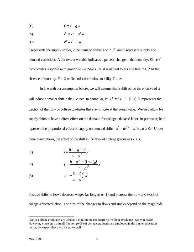
(F) f wξ γ= +& & &

(S) S S Ss wξ γ= +&& &

(D) Ds wζ η= −&& &

? represents the supply shifter, ? the demand shifter and ?, ?S, and ? represent supply and

demand elasticities. A dot over a variable indicates a percent change in that quantity. Since ?S

incorporates response in migration while ? does not, it is natural to assume that ?S ≥ ?. In the

absence of mobility ?S = ?, while under frictionless mobility ?S→∞.

In line with our assumption before, we will assume that a shift out in the F curve of ξ&

will induce a smaller shift in the S curve. In particular, let Sξ λξ=& & , λ∈[0,1]. λ represents the

fraction of the flow of college graduates that stay in state at the going wage. We also allow for

supply shifts to have a direct effect on the demand for college educated labor. In particular, let δ

represent the proportional effect of supply on demand shifts: ξδλξδζ &&& == S , δ ≥ 0.3 Under

these assumptions, the effect of the shift in the flow of college graduates (ξ& ) is:

(1) ξγη

λδγηλ &&S

S

s++

=

(2) ξγη

γλδγη &&S

Sf

+

−−+=

)1(

(3) ξγη

λδ &&S

w+

−−=

)1(

Positive shifts to flows decrease wages (as long as δ<1) and increase the flow and stock of

college-educated labor. The size of the changes in flows and stocks depend on the magnitude

3 Since college graduates are used as a input in the production of college graduates, we expect δ≥0. However, since only a small fraction (0.05) of college graduates are employed in the higher education sector, we expect that δ will be quite small.

May 9, 2001 7

of supply and demand elasticities.

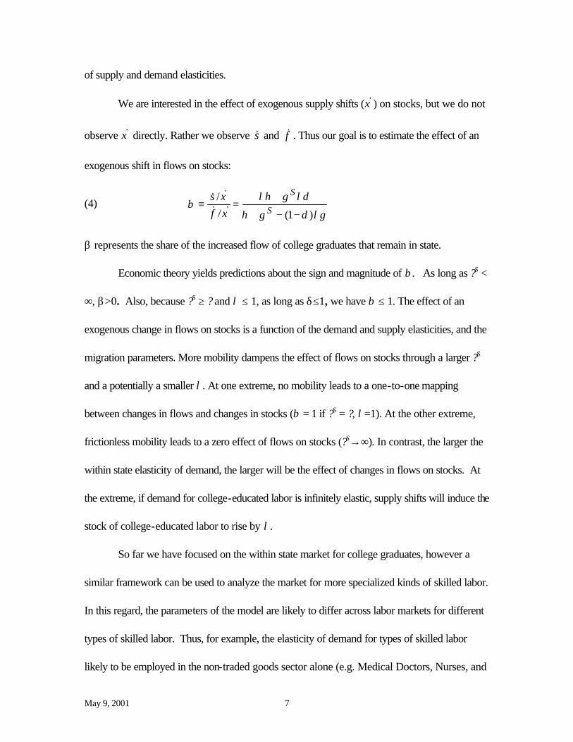
We are interested in the effect of exogenous supply shifts (ξ& ) on stocks, but we do not

observe ξ& directly. Rather we observe s& and f& . Thus our goal is to estimate the effect of an

exogenous shift in flows on stocks:

(4) λγδγη

λδγληξξ

β)1(/

/

−−+

+=≡ S

S

fs

&&&&

β represents the share of the increased flow of college graduates that remain in state.

Economic theory yields predictions about the sign and magnitude of β . As long as ?S <

∞, β>0. Also, because ?S ≥ ? and λ ≤ 1, as long as δ≤1, we have β ≤ 1. The effect of an

exogenous change in flows on stocks is a function of the demand and supply elasticities, and the

migration parameters. More mobility dampens the effect of flows on stocks through a larger ?S

and a potentially a smaller λ. At one extreme, no mobility leads to a one-to-one mapping

between changes in flows and changes in stocks (β = 1 if ?S = ?, λ=1). At the other extreme,

frictionless mobility leads to a zero effect of flows on stocks (?S→∞). In contrast, the larger the

within state elasticity of demand, the larger will be the effect of changes in flows on stocks. At

the extreme, if demand for college-educated labor is infinitely elastic, supply shifts will induce the

stock of college-educated labor to rise by λ.

So far we have focused on the within state market for college graduates, however a

similar framework can be used to analyze the market for more specialized kinds of skilled labor.

In this regard, the parameters of the model are likely to differ across labor markets for different

types of skilled labor. Thus, for example, the elasticity of demand for types of skilled labor

likely to be employed in the non-traded goods sector alone (e.g. Medical Doctors, Nurses, and

May 9, 2001 8

teachers) is likely to be quite small. In such cases, we expect the effects of flows on stocks to

be minimal. We have suggested that for BAs δ, the proportional effect of shifts in the supply of

college-educated labor on demand, is likely to be small. However it seems likely that in some

cases (e.g. for Ph.Ds) δ might be reasonably large, owing to potentially strong

complementarities between doctorate training and R&D activities of firms. What is more, a

large fraction of PhDs in the labor market are employed by universities and are used in the

production of PhDs and other university-trained workers. Furthermore, in cases where the

local supply elasticity (γ) is likely to be small (e.g. Medical Doctors), one might expect that

employers and schools would work together to create institutions that would facilitate

geographic mobility.

Section 2: Empirical Strategy and Data

Estimating Equations

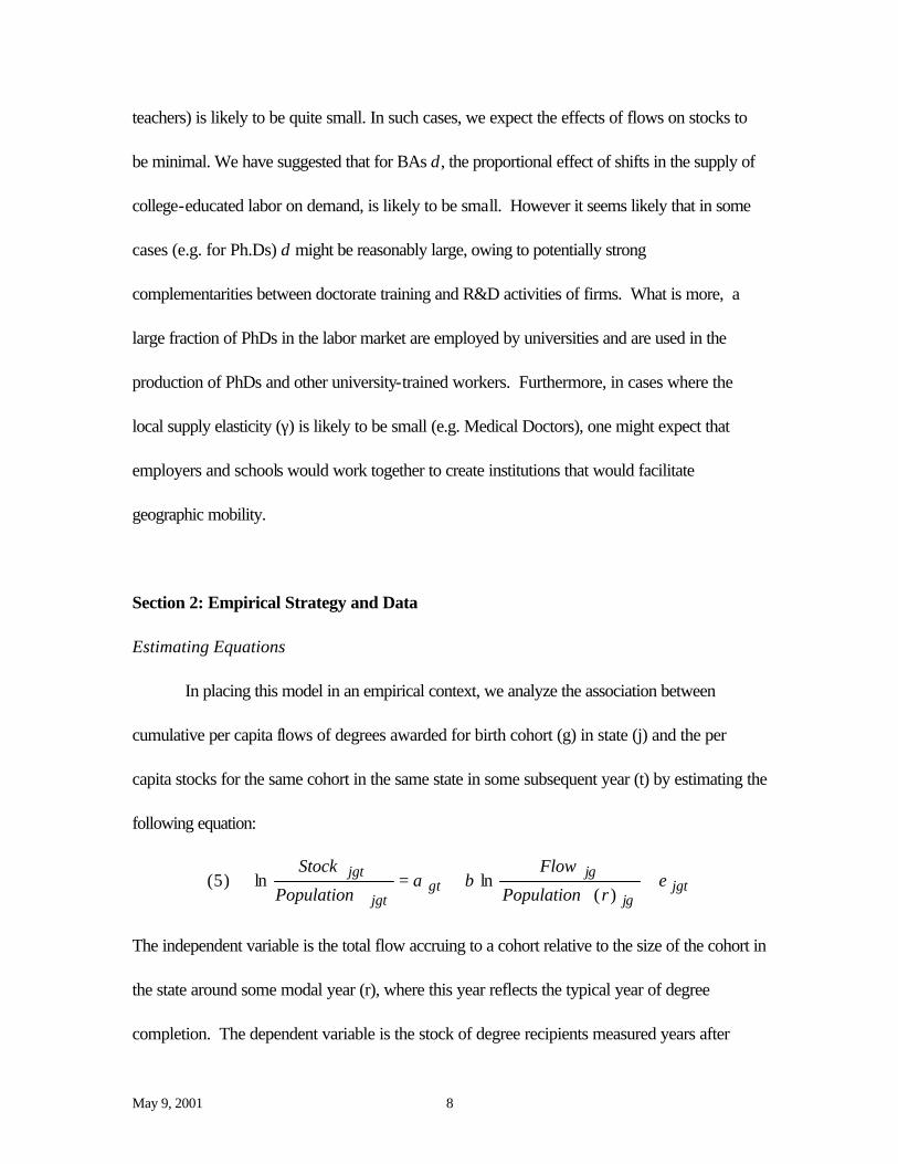
In placing this model in an empirical context, we analyze the association between

cumulative per capita flows of degrees awarded for birth cohort (g) in state (j) and the per

capita stocks for the same cohort in the same state in some subsequent year (t) by estimating the

following equation:

jgtjg

jggt

jgt

jgt

rPopulation

Flow

Population

Stockεβα ++=

)(lnln )5(

The independent variable is the total flow accruing to a cohort relative to the size of the cohort in

the state around some modal year (r), where this year reflects the typical year of degree

completion. The dependent variable is the stock of degree recipients measured years after

May 9, 2001 9

degree conferral for each cohort relative to the population in the state. We present estimates for

different degree types and age groups of observation. The parameter β̂ estimated from

running the cross-sectional equation in (5) corresponds to the theoretical specification outlined in

(1)-(4).4 In this specification, the (intended) identifying variation in the measure of flows reflects

long-standing differences across states in the outputs of higher education institutions,

represented by cross-state variation in ξ. These cross-sectional measures are intended to

capture long-run equilibrium effects on the concentration of college-educated workers in a state

attributable to differences in the outputs of higher education across states.

While we would like to be able to measure the effect of exogenous supply shifts (i.e.

exogenous shifts in flows) on the utilization of college-educated labor within a state, what we are

able to estimate is the cross sectional association between variation in stocks and flows. The

relationship between the coefficient we estimate and the parameter we would like to estimate

depends on what is driving the cross sectional variation in stocks and flows.

There is considerable variation across states both in terms of the production (flows) and

the use (stocks) of college graduates. Some states have -- loosely speaking -- a comparative

advantage in producing college-educated labor. This comparative advantage could come from

such sources as historical forces affecting the location choice of colleges more than a century

ago, proximity to population centers, or willingness of voters to support higher education. In the

labor market, other states presumably have a comparative advantage in the production of goods

and services that are intensive in college-educated labor. The nation’s political and financial

4 The unit of the static model (5) is the state-cohort cell. As discussed in more detail with the

presentation of the empirical results, the inclusion of year effects means that variation across states is what

May 9, 2001 10

capitals (D.C. and N.Y.C.) might be examples of this kind of phenomena.

The variation across states in terms of stocks and flows depends on the combination of

these two factors. If there were variation in states’ comparative advantage for production but

not the use of college-educated labor, we would expect to see that the states that produced the

most educated labor would, uniformly, be the states that used the most educated labor. Market

forces would tend to induce those trained in high production states to emigrate, but this

phenomenon would not change rank orderings. In this case we would expect to find a negative

association between both stocks and flows and relative wages. In contrast, if there were

variation in states comparative advantage in the use, but not in the production of college

educated labor we would still expect to see a very high rank order correlation between states

the produced a lot and states that used a lot of college-educated labor. In this case, we would

expect to find a positive correlation between both the production and the use of college-

educated labor and the relative wages of this group; however, causation would run from the

labor market to the education market.

In fact, what we observe is that some of the states with highly educated workforces also

produce a disproportionate share of college graduates, while others import college graduates.

Likewise, some of the states that produce a disproportionate share of college graduates also

have a disproportionate share in their work forces, while others export college graduates. This

is consistent with the notion that there is cross state variation in the comparative advantage in

both the production and use of college graduates. The implication of these potential sources of

variation across states for our estimates of β̂ is that cross-state differences in demand for

identifies our estimates. Estimated standard errors allow for arbitrary clustering of residuals across states.

May 9, 2001 11

educated labor will tend to bias estimates of β upwards [Appendix A presents an algebraic

derivation of this result]. The more exogenous variation across states in the demand for college

educated labor there is, the greater will this bias be. On the other hand, the more exogenous

variation across states in the supply of college educated labor, the less the bias will be.5

In addition to the cross-sectional analysis we investigate how changes in cohort specific

flows translate to changes in cohort specific stocks. We look at changes between 1960 and

1970, 1970 and 1980, and 1980 and 1990. Here, the focus is on differences in the measures of

flows and stocks over ten-year intervals defined for people of the same age referenced by birth

cohort g and g-10 in a state (j). Again, we present the relationship in an elasticity form:

jgtjgt

jgtgt

jgt

jgt

rPopulation

Flow

Population

Stockεβα +∆+=∆

)(lnln (6)

,

where ∆ means differences between 1970 and 1960, etc. More specifically, for a variable xjgt,

the ten-year difference ∆xjgt is defined as

∆xjgt = xj,g,t – xj,g–10,t–10 ,

where g identifies birth cohorts, measured as year of birth. In this part of the analysis, we focus

solely on the BA measure.

This differenced specification has a somewhat different interpretation than does the

cross-section specification, capturing medium-run dynamic effects rather than long-run

differences. In terms of interpreting estimates as reflecting the causal effects of flows on stocks,

these specifications have the advantage of eliminating state-specific fixed effects. Thus, the

5 These propositions echo standard results on the bias obtained when one uses OLS to estimate

demand of supply curves (Working, 1927).

May 9, 2001 12

variation that we hope to consider in identifying our parameters is the extent to which

idiosyncratic changes in a state’s degree output in higher education have sustained effects on the

concentration of college-educated workers in the population. Still, one concern is that causality

is running in the reverse direction with changes over time in the state-specific demand for college

educated labor feeding back into changes in the fraction of the college-aged population

receiving a degree.

At first blush, one might imagine that the medium run impact of any flow changes should

be larger than the long run impact. After all, we expect the migration elasticity to be larger in the

long as against the medium run. However, the demand elasticity will also be less elastic in the

medium as against the long run, and it is the combination of these two parameters that determine

the medium and long run equilibrium. More concretely, one might imagine that in the medium

run, labor is more mobile than capital, while in the long run, the opposite might be true. In such

a case, the medium run effect of flows on stocks might be smaller than the long run effects.

For both the cross-sectional and dynamic specifications, we present results and

analyses at different degree levels (BA and MD). To the extent that there are well-defined links

between particular fields of study and sectors of employment in the labor market (such as the

case of engineering), we present these stock-flow analyses by field.

Data

The data used in this analysis are from the decennial Census surveys and annual

institutional surveys of degrees awarded by colleges and universities conducted by the

Department of Education (further details are available in the Data Appendix). For each degree

type, we aggregate across institutions to obtain the number of degrees of each type awarded

May 9, 2001 13

per year in each state. To obtain measures of per capita flows for each cohort, we distributed

degrees awarded in each state and year across cohorts following the procedures detailed in the

appendix and then divided these imputed cohort specific flows by an appropriate age-specific

measure of population. For BA degree recipients, the population variable at age 22 is

calculated from widely-available tabulations of the age distribution in a state, made available by

the Census Bureau. This procedure undoubtedly introduces a certain amount of error in our

flow measure. Since there is substantial stability in state-specific flows across time, these errors

are unlikely to have any substantial effect on our cross-sectional estimates. We were worried,

however, that they would have substantial effect on our dynamic estimates. To gauge the

magnitude of this problem, we have done a number of simulations, which suggest that the

magnitude of the bias introduced by the imputation error is relatively small – on the order of

10%.6

For MD data only, we are able to organize information by birth cohort so we are able

to mitigate some of the measurement problems associated with the timing of degree receipt for

this group. The data for MD degree recipients is from a database maintained by the AMA that

records age and other demographic characteristics, institution of degree receipt, and

professional employment location. We observe this universe in 1980 and 1991 and are

therefore able to make overtime comparisons as well as cross-sectional comparisons.

To estimate the per capita stock of college graduates at the baccalaureate level in a

state we use micro data from the decennial census for years 1960, 1970, 1980, and 1990. We

6 Further discussion of these issues together with the results from the simulations are available

upon request from the authors.

May 9, 2001 14

calculate the share of BA recipients in an age group relative to the population size as our age

measure. The 1990 Census provides an advantage over previous decennial files for this analysis

because degree levels are coded explicitly, rather than presenting years of completed education.

For earlier census years (1960-1980), we make the standard assumption in equating college

graduation with 16 years of completed education. The 1990 Census identifies both the state in

which a person lives and, for those that work, the state in which they work. 7 Earlier Census

enumerations either do not identify state of work, or do so for a subset of the sample. For

consistency sake all results we report are based on state of residence. We did, however

replicate our 1990 cross sectional results classifying individuals according to the state in which

they work. Switching to state of work made virtually no difference to any of our results.

Among MDs, we use data from the AMA database on degree receipt to measure the

numerator and data from the Census to measure the denominator or cohort size.

In the cross-sectional analysis, we present data for a long range of age cohorts or

degree receipt years, as well as several ten-year age groups to determine whether the stock

flow relationship differs with age. For the dynamic analysis, we compare individuals of the same

age at different points in time. Because our differences in stock observations are linked to the

decennial census data, we use ten-year differences in age groups.

Section 3: Concentration of Flows and Stocks

7 We limit the analysis to the 48 continental states as data for Alaska and Hawaii are often difficult

to obtain in early years and the obvious differences in geographic integration may lead to somewhat different dynamics. In most cases, we present estimates without DC as the unusual political and industrial structure of this area often leaves this case an outlier.

May 9, 2001 15

The starting point for the empirical analysis is the consideration of the concentration of

flows and stocks across states and the population. We begin with the consideration of those

receiving degrees between 1966-1985; for BA degrees this reflects the 27-46 age group and

for MDs the 32-51 age group (Table 1). The mean flow and stock measures, presented in the

first column are indicative of degree receipt, with BA degree recipients nearly 75 times more

prevalent than MDs. A focal measure of our analysis is the coefficient of variation, which

captures the dispersion relative to the mean. A low coefficient of variation is indicative of

relatively uniform degree production across states while a high coefficient of variation is

indicative of large cross-state differences in degree production. Across degree types, the

dispersion in flows of BA degrees is much less than for MDs.

This dispersion is evident geographically when maps of the flow level by states are

considered in Figure 2. At the BA level, the plains states and northeast states are particularly

strong producers in higher education. States like New Hampshire, Vermont, and

Massachusetts in the East have nearly twice the per capita flow as states like Georgia, South

Carolina and California at the BA level. Turning to the production of MD degrees, there is

appreciably more variation across states in the production of degrees. At one extreme, states

that are not densely populated such as Montana, Idaho, and Wyoming do not record any

institutions awarding the MD. At the other, states such as New York, Illinois and Iowa report

relatively high production of MD degrees. A second type of disaggregation is within field in the

May 9, 2001 16

BA degree category.8 Engineering, and industry-specific fields within engineering, are more

geographically concentrated than BA degrees more generally.

Table 1 also presents the analysis of variance for the stock and flow measures,

considering variation over time, across states, and within states for BA degrees in aggregate,

engineering BAs and the component fields, and medical degrees. Decomposing the observed

variance for the two decades of state-level observations reveals that the bulk of the variation is

consistently across states. For example, at the BA degree level, about 77 percent of the

observed variation in flows is across states. Such persistence in the difference in the production

of degrees awarded points to the presence of long-run differences across states in the

production of degrees awarded. In fact, these cross state differences have been quite persistent

over the entire 20th century. The map showing the dispersion of flows in 1929 (Figure 2,

bottom left) is remarkably similar to the more recent distribution of flows in the top panel of

Figure 2 and with the correlation between the two being 0.5.9

Explanations for these long-term differences across states include factors related to the

historical evolution of higher education across the states, as well as differences across states in

their comparative advantage in degree production. The strength of the eastern states in the

production of BA degrees can be traced to the relatively intensive concentration of private

colleges, many formed before the Civil War by denominational organizations, in this part of the

country. The passage of the Land Grant College Act, commonly known as the first Morrill

8 We do not produce a full stock-flow analysis in all of the fields, as we are only able to construct

appropriate stock measures when field of study and occupation are closely coupled. 9 The two maps suggest a certain amount of convergence between 1929 and the post World War II

period. Indeed, the coefficient of variation across states drops by a factor of two between 1929 and the current period.

May 9, 2001 17

Act,10 in 1862 provided the first large-scale federal support for public provision of higher

education and placed colleges and universities in states that some might have regarded as too

small to support a college of efficient size (Jencks and Reisman, 1968). Geographic

specialization and complementarities with local industry provides another explanation for the

dispersion of colleges and universities across states. For example, it is surely easier to provide

instruction in geology or agriculture in areas that are non-urban, while other clinical fields like

nursing or social work benefit from proximity to densely populated areas. Moreover, the

composition and preferences of the population within a state during the early part of the century

shaped the willingness of state governments to invest in the expansion of public higher education.

Goldin and Katz (1999) suggest that the level of income in a state and the degree of

homogeneity (in terms of religion, ethnicity and income) in the early 20th century were important

indicators of state-supported expansion of colleges and universities. A key point to take from a

brief discussion of the history of higher education is that the distribution and scale of colleges

and universities across states reflects a range of factors including the founding of private colleges

in the 18th and 19th centuries, the willingness of local populations to support public expenditures

on higher education, the introduction of federal support through the land-grant colleges, and the

industrial composition of a state. Some of these factors would seem largely exogenous to state

labor markets, while others are clearly not. To the extent that the observed variation across

states in the degree outputs of colleges and universities reflects historical factors independent of

demand in local labor markets, cross-sectional ordinary least squares estimates can be

10 This bill granted each state thirty thousand acres for each senator and representative in

Congress and the proceeds from this land resource were to be used to fund at least one college.

May 9, 2001 18

interpreted as causal. However, if historical differences in demand for college-educated

workers are substantially related to collegiate degree outputs, cross-sectional estimates will be

upward biased.

Section 4: Stock-Flow Analysis

Cross-Sectional Analysis

While the concentration in the production of university-educated workers and the

concentration in location are readily evident from measures of dispersion, the analytic question

of interest is the impact of flows on stocks. Table 2 presents estimates in elasticity form of the

cross-sectional link between flows and stocks, represented by equation (5). In the category of

BA level flows and stocks, there is a modest association between flow and stock, with an

elasticity of 0.32. Plainly, states with relatively high production of undergraduate students also

have relatively high concentrations of the university-educated in their working age populations.

Yet, this relationship is appreciably less than 1:1. At the other extreme, the cross-sectional

relationship between the production of MD degrees and the representation of MDs in the

population is remarkably weak, with an elasticity estimate very close to zero. The comparisons

across degree types highlight the quite different labor market faced by university-educated labor

with different levels of training. The weak link between flows and stocks in the MD field is

surely indicative of the non-traded aspect of medical services and the associated inelastic

demand within a geographic area. This is not to say, however, that the MDs are equally

distributed across the country or within states. Rather, the link between stock and flow is much

weaker than it is among other degree types.

May 9, 2001 19

Graphical presentation of flows and stocks helps to sharpen the understanding of these

estimates. Each panel in Figure 3 represents the stock-flow relationship averaged over the

1966-85 degree cohorts, with the diagonal line distinguishing net importers (above) and net

exporters (below). For the stock and flow of BA degrees, states such as California and

Connecticut are BA importers while other states like Utah and Vermont consistently export

baccalaureate-trained personnel.11 The picture for MDs is striking in the lack of association

between flows and stocks, as the line showing flows is essentially flat, with the pattern of stocks

across states approaching a straight line at the level of abit more than 4 MDs per thousand.

Turning to the engineering fields at the BA degree level in the bottom panel of Table 2,

the estimated elasticities are positive, with the magnitudes varying appreciably by subfield. As

we will discuss more below, scatter plots reveal a number extreme outliers in the data. We

present results with and without these outliers and the presentation of alternatives without the

outliers is intended to simply show the impact of these cases.12 In subdisciplines like aerospace

and chemical that are likely to be closely linked to industry, the magnitudes of the stock-flow

relationship are much higher than in fields like civil engineering, where demand is likely to widely

dispersed geographically. What we see in the graphical presentation in Figure 4 is a relatively

strong link between stock and flow in sub-fields like aerospace, chemical and mechanical where

the geographic concentration of firms hiring a substantial fraction of these workers is likely to be

sizable. For example, Washington state, Missouri and California dominate aerospace; Michigan

11 Looking at this picture divided by cohort (not shown), demonstrates some consistency

indicative of the measurement of long run equilibrium, as well as variation over time, with states like Washington shifting from a relative exporter of BA-level workers in the early decades of observation to a relative importer in the 1980s and the state of Arizona demonstrating the opposite shift from relative importer to exporter.

May 9, 2001 20

and the Great Lakes states dominate in automobile production; and the location of the DuPont

company in Delaware is a magnet for chemical engineers. Civil engineers, often with

specializations in transportation construction which might be thought of as widely-dispersed in

demand, demonstrate little connection between stocks and flows. Caution against the

overinterpretation of these cross-sectional measures is nonetheless in order as it may well be the

case that universities develop applied engineering programs in response to local demand, rather

than the supply of engineers affecting the location choice of firms.

The examination of outliers in the flow-stock relationship among engineers reveals

considerable information about the geographic integration of the labor markets for specific skills.

One notable class of outlier includes states like South Dakota, North Dakota, Wyoming and

Montana which, on a per capita basis, are quite substantial producers of engineers. Yet, as

shown in Figure 4, these states “export” a substantial share of their college graduates in these

fields and, not surprisingly, dropping the outliers in production from the cross-sectional

regressions serves to drive up the estimated effect of flows on stocks. A different type of outlier

is represented by states with a dominant industry intensive in the employment of engineers, with

examples including the employment of aerospace engineers in Washington state or chemical

engineers in Delaware. In both cases, while these states produce a substantial number of

engineers, they must also attract college-graduates with these skills from other states.

Calculating stock-flow relations for different age ranges and at different points in time

for all BA degrees underscores the persistence of the basic result. Table 3 presents cross-

sectional estimates with stocks observed in 1970, 1980, and 1990 as well as disaggregation of

12 Outliers were identified visually from the scatter plots presented in Figure 4.

May 9, 2001 21

the stock variable into ten-year age groups. The point estimates of the stock-flow relationship

are notably consistent, with only modest variation around the overall cross-sectional result of

0.32 presented in Table 2.

If states with industries that have historically hired a disproportionate share of college

graduates are those that have invested in producing a supply to match the demand, the cross-

sectional estimates will be biased upward. Instrumental variables estimation provides a strategy

to isolate the causal effect of the production of college-educated workers on the long-term

stock. At issue is the identification of factors that might exogenously affect the production of

college-educated labor in a state but that can also be thought to be independent of labor market

conditions. For our cross-sectional estimates, where we are considering relatively permanent

differences across states, we use historical dimensions of the higher education industry and

demographic differences across states to try to isolate factors that affect production today but

that are exogenous to contemporary developments in the labor market. The first type of

instrument is motivated by the observation that large cross-state differences in the degree

outputs and mission of colleges and universities were set in place by state policies well before

World War II. In this regard, we employ the per capita flow of BA degrees in 1929 as one

cross-sectional instrument in this analysis. Presented in Figure 2 (bottom left), the historical

pattern of variation is quite evident. As an alternative instrument we have used a version of the

ethnic diversity measure used by Alesina, Baqir, and Easterly (1999) in their work on public

expenditures (bottom right panel).13 The notion here is that ethnic diversity lowers the

13 The computation of this index is discussed in the data appendix.

May 9, 2001 22

willingness of voters in a state to support public expenditures. The simple correlation between

the diversity index and the historical BA flow measure is -0.36.

Cross-sectional instrumental variables estimates are presented in Table 3, with

appropriate comparisons to the OLS estimates. Column (2) and column (3) present estimates

with the single instruments of BA production in 1929 and racial disparity in 1960. If anything

the IV estimates tend to be somewhat larger than the corresponding OLS estimates, though the

IV estimates tend to be somewhat imprecise and the differences between the OLS and IV

estimates are not statistically significant. The IV estimates thus support the notion that there is a

modest (causal) relationship between flow and stock. Nevertheless, we are cautious in our

interpretation of these IV estimates. In the context of the 1929 BA flow variable, we are

essentially using a long lag in the explanatory variable of BA flows as an instrument for flows

observed for cohorts in our data. Plainly, the validity of this strategy relies on the assumption

that there is no serial correlation in the outcome measure. If there is a substantial correlation

between the industrial composition of a state in 1929 and 1990 that is driven by something other

than the educational attainment of the population – as we would expect -- then the IV estimates

will tend to overestimate the causal effect of flows on stocks just as the OLS estimates do.

At first blush the racial disparity index might seem more plausibly exogenous. Still an

issue arises as to just how long the arm of history is. As can be seen quite clearly in the bottom

panel of Figure 2, the states that rank highly on the disparity index are the states of the

Confederacy. Thus, one interpretation of our results would point to the legacy of slavery, with

racial divisions in the South affecting the willingness of populations in these states to invest in

higher education. On this account, the division of the U.S. into slave and free states may have

May 9, 2001 23

had very long run effects on the economies of the North and the South, but is exogenous to

other factors currently influencing regional economies. However, one can tell a quite different

story. Presumably, the reason that Northern states eliminated slavery early while the Southern

States did not was not primarily because Northerners were morally superior to Southerners, but

because the industrializing economy of the North did not lend itself to a slave based economy.

Thus, on this account, the racial disparity index is correlated with long standing differences in

industrial structure and, as such, cannot be thought of as entirely exogenous.

The overall conclusion that follows from the analysis of the relationship between stock

and flow among BA recipients is that there is a persistent and significant link between BA

degrees awarded and the representation of college-educated in the state. While it is plausible

that part of this difference is indicative of other long-run differences in the structure of local

economies, the persistence of these results do support the link between higher education and the

labor market. Nevertheless, the magnitude of this link is appreciably less than one and

theoretical information about the link between demand and supply would point to an upward

bias in the estimated effects.

Variation in relative wages across states with the concentration of college-educated

workers provides another indicator of the degree of mobility in the labor force and the direction

of the causal relationship between flows and stocks. Table 4 presents estimates of the

regression of relative wages for college graduates on the concentration of college graduates at

the state level for different decennial points of observation. The first column uses the observed

concentration of college graduates as the explanatory variable and column (2) uses the

aggregate of flows (from 1950 to the indicated year) as an instrument for stock to capture

May 9, 2001 24

variation attributable to differences in the flow from the higher education market. In the

presence of an integrated labor market in which labor adjusted fully in location to changes in

demand, these coefficients would be uniformly indistinguishable from zero. Yet, particularly in

the instrumental variables estimates, these estimates are consistently negative, implying an

inverse relationship between flows and relative wages.14 This result is consistent with a situation

in which some states have a comparative advantage in production in the higher education

market, while others have a comparative advantage in the use of college-educated labor and

labor is, even in the long run, not perfectly mobile across states.15 College graduates residing in

states that produce a relatively large number of college graduates per capita tend to earn

relatively little, while college graduates in states that employ a large number of college graduates

but do not produce a large number tend to receive something of a wage premium.

If the flows used as instruments in these specifications are exogenous, the coefficients

reported in the 2nd column of table 4 can be interpreted as -1/η. If, however flows are

endogenous, the reported coefficients will tend to underestimate the causal effect of relative

supply on relative wages16 and, as a result, will tend to overestimate η.

Taking the estimates in the second column of the table at fact value (i.e. interpreting them as

14 Table 4 also presents estimates using the instruments of 1929 BA Flows and the racial diversity

index discussed later in conjunction with Table 3. These results, presented in Column (3) and (4), are qualitatively similar to those presented in (2).

15 If college graduates have a preference for living near other college graduates, then one might find the college wage premium to be low in states with a high concentration of college graduates. In this case, the high premium in states with relatively few college graduates would reflect a compensating differential for living in such areas. Such preferences could rationalize an association between the stock of college graduates and relative wages. This explanation does not, however, rationalize an association between the flow of college graduates and relative wages.

16 If flows are endogenous, then the regression of stocks on flows will tend to over estimate the causal effect of flows on stocks. Similarly, in this case the regression of relative wages on flows will tend to underestimate the causal effect of flows. The IV estimates are the ratio of these two estimates, and therefore will tend to underestimate the causal effect of stocks on relative wages.

May 9, 2001 25

estimates of -1/η), suggests a within state relative demand elasticity in the neighborhood of 5.

These estimates are all substantially larger than comparable estimates using U.S. times series

data (Katz and Murphy, 1992), suggesting that there is considerable reallocation of production

across states to take account of cross state differences in the relative supply of college

graduates. However, it also seems clear that even in the long run, within state relative demand

elasticities are well bellow infinity. Exogenous, cross state differences in the supply of college

graduates are accommodated by the out migration of college graduates and the drop in their

relative wages as well as by demand shifts. In fact, our estimates would seem to suggest that

migration plays a larger role in accommodating supply shifts than do shifts in demand.

Dynamic Analysis

Beyond comparing flows and stocks in the cross-section, the consideration of the

relationship between these measures overtime provides some leverage on the question of

causation. Difference estimates plausibly eliminate fixed differences across states from affecting

the estimates of flows on stocks. These difference estimates capture changes over a relatively

short horizon and thus measure something conceptually different than our cross-section

estimates, which reflect permanent cross-state differences in educational capacity. In this

regard, we ask the question of what happens to the stock of college graduates in a state if the

degree output of the state’s higher education institutions changes at a rate different than the

May 9, 2001 26

national norm for a short interval. The data support this interpretation, as there is not uniformity

in the correlation of changes in flows.17

Table 5 presents the means of the decennial log differences in flows and stocks by age

and period of observation. As is well-known, overall college going expanded dramatically into

the early 1970s, accounting for the large and positive changes in flows for those in the 25 to 34

age range between 1960 and 1970 and between 1970 and 1980. Decreased returns to college

education faced by cohorts making educational investments in the mid and late 1970s

contributed to the decline in flows for the 25-34 age group over the interval from 1980 to 1990.

Turning back to the first table, the analysis of variance numbers give an indication that

variation within states over time is an appreciably smaller share of the total variance than the

cross-sectional differences. However, as Table 5 and Figure 5 indicate, there is still significant

cross state variation in the change in the flows from one decade to the next. Thus, for example,

while on average per-capita flows for 25-34 year olds increased by roughly 25% between

1970 and 1980, the growth ranged from close to 0% for states such as Oregon, Utah,

Wyoming and Nebraska to close to 40% for Florida, Nevada, Alabama and Virginia, over

60% for New Mexico and over 80% for Delaware.

Since it is the per capita flow variable we use in our analysis, changes in this variable can

reflect movements in either the numerator or the denominator. In fact, in our data there is a

strong negative correlation between changes over time in the size of the 22 year old population

and changes in per capita flows. Indeed, regressions of the change in per capita flows on the

17 States that increased relative flows between 1960 and 1970 were not identical to those with

relative increases between 1970 and 1980, though there is a positive relationship between the 1970 to 1980 change and the 1980 to 1990 change. Overall, none of these relationships among flows is very strong nor is

May 9, 2001 27

change in the size of the cohort suggest that a 10% increase in cohort size is associated with 7%

decrease in per capita flows. Statistically, cohort size explains about 25% of the variation in the

change over time in per-capita flows, with this phenomenon more important in some states than

others.

While in our overtime analysis we eliminate permanent cross state differences, the

change over time in per capita flows could still be endogenous to state specific changes in the

demand for college educated labor. When thinking about how serious an issue this is, it is

important to understand that the variation at issue represents differences across states in the

growth of flows from one decade to the next. Since typically growth in one decade is not

followed by growth in the next, it is appropriate to think about the cross state variation as

reflecting variation in the timing of the growth in flows. All states experience a dramatic increase

in the fraction of their college aged population attending and finishing college between 1950 and

1970, however, the timing of these increases varied across states. We suspect that the timing of

these changes is largely exogenous to changes in the demand for college-educated labor. The

actions of governors in the sphere of higher education are one such potentially exogenous force.

To give but one example, the expansion of higher education in New York state under

the gubernatorial terms of Nelson Rockefeller represents a striking case in point. Few

observers early in the Rockefeller administration would have predicted a six-fold increase in

state funding for higher education in New York state in the decade between 1956 and 1966,

with the increase in New York exceeding the changes in neighboring Connecticut and New

Jersey by 60% and 45%, respectively. Yet, denied a national office with the nomination of

there evidence that they persist over time.

May 9, 2001 28

Nixon in 1960, Rockefeller threw his considerable personal energy and ambition into capital

projects in the state including the transformation of the SUNY system from teachers colleges to

a national-level university system.

While the New York case is a dramatic example of expansion led by the governor,

other examples such as Michigan Governor Milliken’s $50 million reduction in state support for

higher education in 1983 point to public colleges and universities as an open and politically

viable target for gubernatorial budget slashing when faced with revenue shortfalls (Gove, ECS,

1998). Another type of relative contraction in state level higher education is apparent in the

tightly constrained growth of southern systems of higher education during the 1960s, as pressure

to desegregate higher education may have also attenuated political support for colleges and

universities.

While the state political process clearly plays a substantial role in the overtime variation

in the outputs of higher education within a state, the strength of this effect varies appreciably

across states with the composition of public and private institutions. In states such as California

where public institutions constitute the majority provider of higher education, there are likely to

be substantial accommodations to changes in population. Alternatively, in a state like

Massachusetts where higher education has been provided largely by private institutions,

accommodations in degree outputs to population growth or political pressure are likely to be

more muted. To put this in perspective, 74 percent of BA degrees awarded in California in

1988 were awarded by public institutions compared to 32 percent in Massachusetts during this

year. Not surprisingly, the examination of residuals in a regression predicting flows with state

May 9, 2001 29

and year effects indicates that in Massachusetts periods of rapid population expansion were met

with below average flows.

These kinds of considerations lead us to suspect that there is considerable exogenous

variation in the state-specific changes over time in per capita flows. This, of course, does not

mean that all of the variation is exogenous. Just as was true in the cross section, if part of the

state-specific variation over time in flows represents a response to labor market conditions, then

our ols estimates will tend to over-estimate the causal impact of flow changes on stock changes.

Thus, our estimates represent upper bounds on the causal effect of flows on stocks.

Table 6 presents estimates with the decennial change in stock regressed on the

decennial change in flow for different age cohorts. These dynamic estimates, reflecting the

difference presentation from equation (6), use variations over time within states rather than fixed

differences across states to identify the effect of flows on stocks. Estimates for relatively recent

college graduates – those that are 25-34 years old as of the census years – are shown in the

first column. For these cohorts, the difference estimates show significant effects of flow on

stock in the range of 0.37 to 0.44 for the 1960-1970 and 1980-1990 intervals, while the

estimate for 1970-80 is somewhat weaker. Inspection of scatter plots for the 1970-80 decade

revealed two outlier states, Delaware and New Mexico [Figure 5]. Both of these states

showed a dramatic growth in the number of individuals receiving a BA, during the 1960s, but no

corresponding growth in the fraction of the population with a BA Removing these two states

from our calculations (columns (4)-(6)) produces results for this cohort that are much more in

line with results for other cohorts and that show statistically and quantitatively large associations

May 9, 2001 30

between changes in flows and changes in stocks [0.31 (0.08)].18 However, we want to

emphasize here, as well as elsewhere, that we think outliers usually contain valuable information.

Here the very fact that despite enormous increase in the number of individuals receiving BAs

from New Mexico and Delaware, the increase in flows did not seem to translate into an

increase in stocks some years down the line. Thus, these outliers would seem to confirm for us

the sense we get from these tabulations that flows have a best a moderate effect stocks.19

Also in this table (columns 2, 3, 5, 6), we present results for older age groups that

would typically have graduated from college more than 10 years prior to the year in which we

observe them. These results would seem to indicate that the relationship between flows and

stocks tends to diminish somewhat as cohorts age, with the elasticity declining to about

0.22(0.07) for the 35-44 age group and then falling further to .08(0.07) for those in the 45-52

age group. When thinking about this diaspora20 of college graduates, it is important to bear in

mind that, typically, the growth in flows in one decade is not 'ratified' by a growth in flows in

following decades. Thus, the impact of a change in flows on stocks two to three decades later

is conceptually distinct from the long run impact of a change in flows (i.e. the kind of quantity we

were attempting to estimate using the cross state variation in flows).

18 For those in the 25-34 age cohort, difference estimates for other cohorts include 0.32(0.10) for

1970-1960 and 0.41(0.06) for 1990-1980 for regressions limited to 46 states and excluding DC, Delaware and New Mexico.

19 Here, and in other places, we see evidence that the impact of flows on stocks in states that are small either in terms of land area or population, tends to be particularly weak. We tried testing such hypotheses statistically by including interaction terms in our models. Generally speaking, the estimates on the interaction terms suggested that the smaller a state the weaker is the association between flows and stocks. However, the estimated interaction terms were generally not statistically significant. Given the sample size we are dealing with (effectively 48 observations), this was hardly surprising.

20 Jim Hines coined this phrase.

May 9, 2001 31

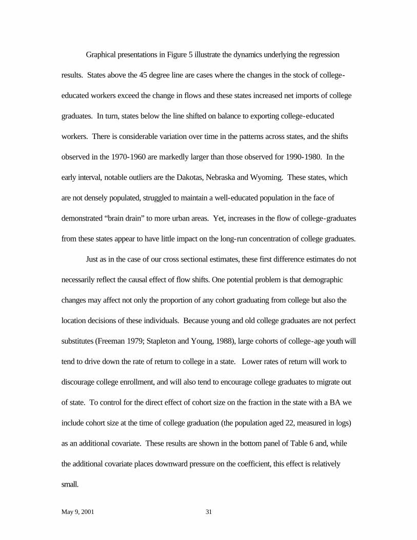
Graphical presentations in Figure 5 illustrate the dynamics underlying the regression

results. States above the 45 degree line are cases where the changes in the stock of college-

educated workers exceed the change in flows and these states increased net imports of college

graduates. In turn, states below the line shifted on balance to exporting college-educated

workers. There is considerable variation over time in the patterns across states, and the shifts

observed in the 1970-1960 are markedly larger than those observed for 1990-1980. In the

early interval, notable outliers are the Dakotas, Nebraska and Wyoming. These states, which

are not densely populated, struggled to maintain a well-educated population in the face of

demonstrated “brain drain” to more urban areas. Yet, increases in the flow of college-graduates

from these states appear to have little impact on the long-run concentration of college graduates.

Just as in the case of our cross sectional estimates, these first difference estimates do not

necessarily reflect the causal effect of flow shifts. One potential problem is that demographic

changes may affect not only the proportion of any cohort graduating from college but also the

location decisions of these individuals. Because young and old college graduates are not perfect

substitutes (Freeman 1979; Stapleton and Young, 1988), large cohorts of college-age youth will

tend to drive down the rate of return to college in a state. Lower rates of return will work to

discourage college enrollment, and will also tend to encourage college graduates to migrate out

of state. To control for the direct effect of cohort size on the fraction in the state with a BA we

include cohort size at the time of college graduation (the population aged 22, measured in logs)

as an additional covariate. These results are shown in the bottom panel of Table 6 and, while

the additional covariate places downward pressure on the coefficient, this effect is relatively

small.

May 9, 2001 32

More directly, we are concerned that the estimated elasticity between flow and stock is

capturing the effect of local demand shocks on flows rather than the effect of supply shocks in

higher education on the concentration of college-educated in the potential labor force within a

state. Including direct measures of demand captured by the employment level in the reduced

form differenced regression (bottom right panel of Table 6) is one avenue to address this

problem and, in this specification, point estimates change only slightly from the original

specification.

The optimal fix would be the employment of exogenous factors that have changed over

time as instruments for changes in flows in our difference specification. Tuition rates at state

universities and colleges would seem an obvious alternative and there is ample evidence that

tuition rates do, indeed, have strong effects on enrollment rates (see Kane, 1999, and the

literature cited therein). However, tuition rates are, themselves, plausibly endogenous to local

labor market developments. Indeed there is some evidence of a relationship between the

strength of state economies and state-specific changes in tuition levels (Kane, 1999), with tuition

levels at state institutions often moving upward in periods of economic contraction. Empirically,

the relationship between tuition levels and cohort completion rates is relatively weak, proving

insufficient to serve as a strong instrument.21

21 Preliminary analysis of the pattern of completion rates indicates that increases in tuition have a

modest and negative impact on completion rates while increases in the unemployment rate are positively associated with college completion in specifications that allow for state and year fixed effects. These estimates are consistent with the estimates reported in Kodrzycki (1999). We have also experimented with two other time series measures of state-level support for higher education as potential instruments: the level of state appropriations and the number of institutions of higher education in the state. Results based on these instruments were not more satisfactory that the estimates based on tuition.

May 9, 2001 33

Examination of the dynamic relationship for available cohorts in the engineering medical

fields suggests a somewhat different story than is evident for BA degree recipients in general.

What we find in the case of engineers as evidenced by the string of uniformly small and

insignificant estimates in Table 7 is that changes in flows do not appear to affect changes in

stocks (with the exception of the aerospace sub-field). These results are consistent with the

notion that for engineering, at least in the medium run, within state demand curves are quite

inelastic. One plausible explanation for this would that, in the medium run, the location of

production for establishments employing engineers is geographically relatively immobile. This

would be true if the industries in question showed increasing returns to scale and if their were

also substantial geographic mobility costs for the industry (Krugman, 1991). At any rate, it

appears that states with industries intensive in the employment of engineers will continue to draw

these college-educated workers, regardless of the source of production. The state of

Washington in aerospace engineering and the state of Delaware in chemical engineering are

notable examples of this phenomenon, as both are plainly intensive in engineering and increase

their stocks at a rate greater than their flows [see Figure 6]. One result, which carries over from

the cross-sectional analysis, is the persistent out-migration of engineers trained in states like

Montana and North Dakota. While these states experienced among the largest growth in the

flow of engineers, the representation of workers with these skills in the changed very little over

time.

For MDs, the evidence presented in Table 8 indicated that there is a positive and

significant relationship between changes in flows and changes in stocks. Close inspection of the

data reveals (see Figure 7) a clear and compelling story. States that had the largest changes in

May 9, 2001 34

flows tended to be states like West Virginia and South Dakota that may have been underserved

in medical care at the beginning of the interval. As such, adding a medical college in West

Virginia is one policy remedy to increase the supply of doctors in the state. For example, the

state of West Virginia has two universities recently established programs awarding

medicaldegrees: the West Virginia University School of Medicine (part of the Robert C. Byrd

Health Sciences Center) and the Joan C. Edwards School of Medicine at Marshall University.22

Both institutions have mission statements that explicitly address the need to provide physicians

and medical personnel for underserved areas and make explicit reference to recruiting students

from rural West Virginia and placing graduates in clinical practices to improve health care in

West Virginia. In the context of our model, it is likely that the medium term effects of changing

the production of MDs within a state may be relatively large as the additional MDs producedin

a state like West Virginia include many people who are from West Virginia and have a

preference for remaining in the state. Still the absolute magnitudes of the coefficients are small

(0.2) and indicate that for each ten additional physicians trained in the state, only about 2 will

remain in the state’s population for the long term.

Section 5: Conclusion

The empirical evidence in this analysis points to a modest relationship between degree

production in the education market and the concentration of college educated workers in a

state’s population. For the general pool of BA degrees, we estimate the long-term elasticity

22 West Virginia University awarded its first MD in 1962 and Marshall University established its

medical school in 1977.

May 9, 2001 35

between stock and flow to be on the order of 0.3.23 Taking BA degrees in engineering and MD

degrees as special cases, our results point to the nature of demand in the labor market as a

substantial determinant of the stock-flow relationship. For MD degrees, the relatively inelastic

nature of demand within states in long-term equilibrium contributes to the wide dispersion across

states and the relatively weak link between flows and stocks. For engineering fields, it is most

difficult to infer causation from the sizable cross-sectional estimates, as it may well be that

colleges and universities adjust their offers to meet the needs of local industry. The dynamic

estimates, taking advantage of within state variation in output, point to a generally weak link

between the output of such specialized labor and the change in the concentration of workers

with these skills. It may be that, in the medium run at least, capital is less mobile than labor and

the increase in specialized labor within a state is likely to be met be emigration to states with

established industrial centers for the employment of specific skills.

In this regard, our estimates are also suggestive of how state economies adjust to supply

shocks. The labor literature (e.g. Blanchard and Katz, 1992; Borjas, Katz and Freeman, 1997)

have argued for the importance of migration as a means that states have of adjusting to

macroeconomic shocks. Our results suggest that migration does work to mitigate the effects of

shocks to the supply of labor – eliminating roughly more than half of the original impact – but

clearly other adjustment processes are also at work. Workers surely face costs of moving from

one state to another and, in a related point, many have preferences to live near family or friends

from college.

23 This estimate is likely to be an upper limit. It is likely that there is an association between states

with a comparative advantage in the production of college-educated workers and those with a comparative advantage in employment. In this case, our estimates are likely to be biased in an upward direction.

May 9, 2001 36

Our results point to the finding that state policy makers have only a modest capacity to

influence the human capital levels of their populations by investing in higher education. Within

this relatively limited sphere of influence, the structure of specific labor markets – particularly the

elasticity of demand for labor and the relative mobility of capital and labor – will substantially

affect the expected link between degree production in the education market and the

concentration of college-educated workers in the work force. What is far less clear from the

analysis is how policy makers should evaluate the payoff to modest increments in the size of the

population with BA degrees.24 Even if there are no externalities in the form of wage spillovers,

there may well be other types of externalities such as higher tax revenues, improved governance,

or other amenities that make public subsidies in collegiate education a good investment.

24 Efforts to trace out the effects of changes in the production of college-educated labor on state

labor markets have not been terribly successful. The flow and especially the change in flow of college graduates in a state simply does not seem to have a large enough impact on the stock or changes in the stock of college educated workers in a state to allow for meaningful estimation of the effects of these changes on wages. At the heart of this problem is the fact that the workers in a state reflect cohorts of workers that entered the labor market over more than a half century of time. Presumably this is a problem not just for our attempts to estimate the effect of flow of college graduates on labor market outcomes, but also for others attempts to do so. The evidence concerning whether states with relatively high wages are those in which college-educated workers are used relatively intensively is inconclusive. Our capacity to identify such equilibrium agglomeration effects is confounded by the presence of demand shocks that do not appear to be fully dissipated in the labor market. As such, evidence that relies on cross-cohort differences is very sensitive to the choice of intervals of estimation. Moreover, variation in the flow of college graduates explains only a modest fraction of the overall variation in the stock of college graduates across states.

May 9, 2001 37

References

Alesina, Alberto; Reza Baqir and William Easterly. 1999. “Public Goods and Ethnic Divisions.” The Quarterly Journal of Economics. Volume 114, No. 4. Angrist, Joshua and Darren Acemoglu. 1999. “How Large are the Social Returns to Education? Evidence from Compulsory Schooling Laws,” MIT mimeo. Bartik, Timothy. 1991. Who Benefits from State and Local Economic Development Policies? W.E. UpJohn Institute, Kalamazoo, MI. Beeson, Patricia and Edward Montgomery. 1993. “The Effects of Colleges and Universities on Local Labor Markets.” The Review of Economics and Statistics. Volume 75, No, 4. Blanchard, Olivier and Lawrence Katz. 1992. “Regional Evolutions.” Brookings Papers on Economic Activity, No. 1, pp 1-61. Borjas, George J.; Richard Freeman, and Lawrence Katz. 1997. “How Much Do Immigration and Trade Affect Labor Market Outcomes?” Brookings Papers on Economic Activity v0 n1 1-67. Bound, John and Harry Holzer. 2000. “Demand Shifts, Population Adjustments, and Labor Market Outcomes during the 1980s.” Journal of Labor Economics, 18:20-54. Card, David and Thomas Lemieux. 2000. “Dropout and Enrollemnt Trends in the Post-War Period: What Went Wrong in the 1970s?” mimeo. Card, David and Thomas Lemieux. 2000. “Can Falling Supply Explain the Rising Return to College for Younger Men?” mimeo. Freeman, Richard. 1979. “The Effect of Demographic Factors on the Age-Earnings Profile in the U.S.” Journal of Human Resources XIV:3. Glaeser, Edward L., Joes A. Scheinkman, and Andrei Shleifer. 1995. “Economic Growth in a Cross Section of Cities,” Journal of Monetary Economics, 36:117-143. Glendon, Spencer, 1998. “Urban Life Cycles.” Harvard University Mimeo. Goldin, Claudia and Larry Katz. 1999. “The Shaping of Higher Education: The Formative Years in the United States, 1890 to 1940.” The Journal of Economic Perspectives, Vol. 13, No. 1 (Winter).

May 9, 2001 38

Hanson, Gordon and Matthew Slaughter. 1999. “The Rybczynski Theorem, Factor Price Equalization, and Immigration: Evidence from the U.S. States” NBER Working Paper 7074. Hanson, Gordon. 2000. “Firms, Workers and the Geographic Concentration of Economic Activity,” in The Handbook of Economic Geography, Oxford University Press. Hanson, Gordon. 2000. “Scale Economies and the Geographic Concentration of Industry,” Journal of Economic Geography (forthcoming). Jaffe, Adam. 1989. “Real Effects of Academic Research.” American Economic Review 79 (5) 957-970. Katz, Lawrence and Kevin Murphy. 1992. “Changes in Relative Wages, 1963-1987: Supply and Demand Factors.” Quarterly Journal of Economics, Vol. 107, No. 1. (February), pp. 35-78. Kodrzycki, Yolanda. 1999. “Geographic Shifts in Higher Education.” New England Economic Review (July/August). Krugman, Paul. 1991. “History versus Expectations.” Quarterly Journal of Economics. Volume 106, No. 2. Long, Larry E. 1988. Migration and residential mobility in the United States. New York: Russell Sage Foundation. Moretti, Enrico. 1999. “Estimating the Social Return to Education: Evidence from Repeated Cross-sectional and Longitudinal Data.” Center for Labor Economics, Working Paper 21. Rauch, James E. 1993. “Productivity Gains from Geographic Concentration of Human Capital: Evidence from the Cities.” Journal of Urban Economics v34 n3 380-400. Rauch, James E. 1993. “Does History Matter Only When it Matters a Little? The Case of City-Industry Location.” Quarterly Journal of Economics, Volume 108, No. 3. Roback, Jennifer. 1982. “Wages, Rents, and the Quality of Life.” Journal of Political Economy. 90:1257-78. Stapleton, David C. and Douglas Young. 1988. “Educational Attainment and Cohort Size.” Journal of Labor Economics v6 n3 330-61. Working, E.J. 1927. What Do Statistical "Demand Curves" Show? Quarterly Journal of Economics, Vol. 41, No. 2. pp. 212-235.

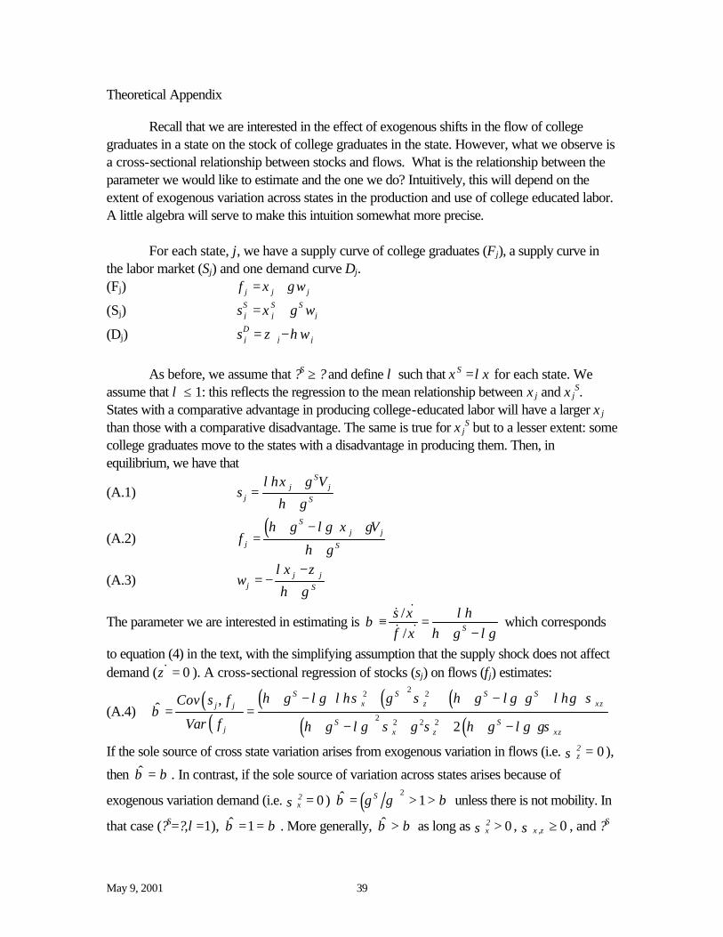
May 9, 2001 39

Theoretical Appendix

Recall that we are interested in the effect of exogenous shifts in the flow of college graduates in a state on the stock of college graduates in the state. However, what we observe is a cross-sectional relationship between stocks and flows. What is the relationship between the parameter we would like to estimate and the one we do? Intuitively, this will depend on the extent of exogenous variation across states in the production and use of college educated labor. A little algebra will serve to make this intuition somewhat more precise.

For each state, j, we have a supply curve of college graduates (Fj), a supply curve in

the labor market (Sj) and one demand curve Dj. (Fj) j j jf wξ γ= +

(Sj) S S Sj j js wξ γ= +

(Dj) Dj j js wζ η= −

As before, we assume that ?S ≥ ? and define λ such that ξS =λξ for each state. We

assume that λ ≤ 1: this reflects the regression to the mean relationship between ξ j and ξ jS.

States with a comparative advantage in producing college-educated labor will have a larger ξ j than those with a comparative disadvantage. The same is true for ξ j

S but to a lesser extent: some college graduates move to the states with a disadvantage in producing them. Then, in equilibrium, we have that

(A.1) S

j jj S

sληξ γ ς

η γ

+=

+

(A.2) ( )S

j jj S

fη γ λγ ξ γς

η γ

+ − +=

+

(A.3) j jj S

wλξ ζ

η γ

−= −

+

The parameter we are interested in estimating is // S

sf

ξ ληβ

η γ λγξ≡ =

+ −

&&& & which corresponds

to equation (4) in the text, with the simplifying assumption that the supply shock does not affect demand ( 0=ζ& ). A cross-sectional regression of stocks (sj) on flows (fj) estimates:

(A.4) ( )

( )( ) ( ) ( )

( ) ( )

22 2

2 2 2 2

,ˆ2

S S S Sj j

S Sj

Cov s f

Var f

ξ ζ ξζ

ξ ζ ξζ

η γ λγ λησ γ σ η γ λγ γ ληγ σβ

η γ λγ σ γ σ η γ λγ γσ

+ − + + + − + = =+ − + + + −

If the sole source of cross state variation arises from exogenous variation in flows (i.e. 02ζσ = ),

then β̂ β= . In contrast, if the sole source of variation across states arises because of

exogenous variation demand (i.e. 02ξσ = ) ( )2ˆ 1Sβ γ γ β= > > unless there is not mobility. In

that case (?S=?,λ=1), ˆ 1β β= = . More generally, β̂ β> as long as 02ξσ > , 0,ξ ζσ ≥ , and ?S

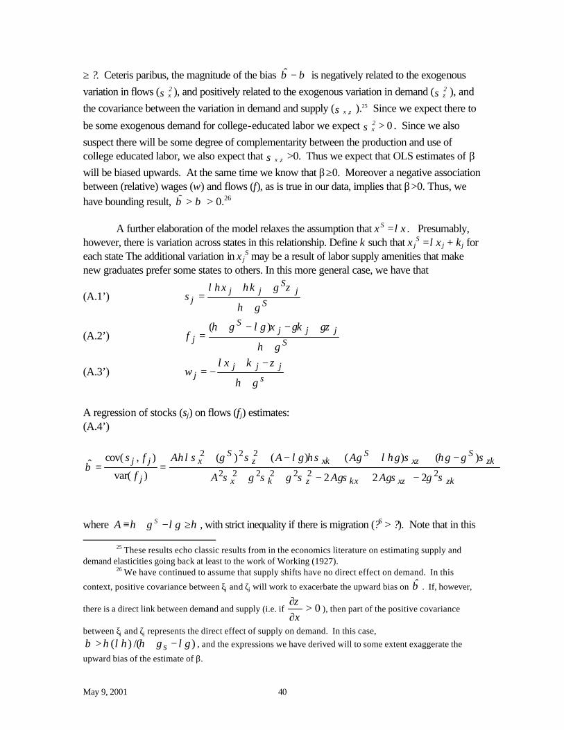
May 9, 2001 40

≥ ?. Ceteris paribus, the magnitude of the bias β̂ β− is negatively related to the exogenous variation in flows (σ ξ

2 ), and positively related to the exogenous variation in demand (σ ζ2 ), and

the covariance between the variation in demand and supply (σ ζξ , ).25 Since we expect there to

be some exogenous demand for college-educated labor we expect 02ξσ > . Since we also

suspect there will be some degree of complementarity between the production and use of college educated labor, we also expect that σ ζξ , >0. Thus we expect that OLS estimates of β will be biased upwards. At the same time we know that β≥0. Moreover a negative association between (relative) wages (w) and flows (f), as is true in our data, implies that β>0. Thus, we have bounding result, β̂ β> > 0.26

A further elaboration of the model relaxes the assumption that ξS =λξ. Presumably,

however, there is variation across states in this relationship. Define κ such that ξ jS =λξ j + κj for

each state The additional variation in ξ jS may be a result of labor supply amenities that make

new graduates prefer some states to others. In this more general case, we have that

(A.1’) S

jS

jjjs

γη

ζγηκληξ

+

++=

(A.2’) S

jjjS

jfγη

γζγκξλγγη

+

+−−+=

)(

(A.3’) s

jjjjw

γη

ζκλξ

+

−+−=

A regression of stocks (sj) on flows (fj) estimates: (A.4’)

ζκξζκξζκξ

ζκξζξκζξ

σγγσγσσγσγσ

σγηγσληγγησλγσγηλσβ 2222222

222

222

)()()()(

)var(

),cov(ˆ−+−++

−+++−++==

AAA

AAA

f

fs SSS

j

jj

where SA η γ λγ η≡ + − ≥ , with strict inequality if there is migration (?S > ?). Note that in this

25 These results echo classic results from in the economics literature on estimating supply and demand elasticities going back at least to the work of Working (1927).

26 We have continued to assume that supply shifts have no direct effect on demand. In this

context, positive covariance between ξj and ζj will work to exacerbate the upward bias on β̂ . If, however,

there is a direct link between demand and supply (i.e. if 0>∂∂ξζ

), then part of the positive covariance

between ξj and ζj represents the direct effect of supply on demand. In this case, )/()( λγγηληηβ −+> s , and the expressions we have derived will to some extent exaggerate the

upward bias of the estimate of β.

May 9, 2001 41

case, 2κσ mitigates the upward bias of β̂ . On the other hand, all of the qualitative results

regarding (A.4) hold if the variation in δ is relatively small, or the covariance supply and demand amenities (σκζ) and the covariance of supply amenities and advantage in higher education (σξκ) are positive.

May 9, 2001 42

Data Appendix The primary sources of data for this analysis are: the decennial Census files, the decennial Census publications, population estimates by the Census Bureau, the October CPS files, institutional surveys of degrees awarded, the National Survey of College Graduates, and the AMA Physician Professional Data. Appendix Table 1 lists specific references. In the paper, we analyze four types of degrees: BAs, Engineering BAs, and MDs. The first part of the appendix is organized by degree type. Steps that apply to all types are discussed with all BAs.

BA Degrees Flows

We wish to compute the per capita flow of college graduates for each state and birth cohort, and the per capita stock of college graduates for each state and cohort for the census years 1960, 1970, 1980, and 1990.

A major measurement problem arises from the fact that, in our baseline data, the stock

variable is defined for birth cohorts, while the flow refers to the year of graduation. Therefore, we had to estimate flows for birth cohorts from the degree-year data. We do not observe the flow of BA degrees awarded to members of birth cohorts directly, but only the sum of degrees awarded to cohorts of different ages. While age 22 is the modal age group for BA recipients, not all BA degree recipients are this age.

First, in each year, we estimated the number of college degrees conferred for different

ages. Using micro data from the October Current Population Survey, we estimated the age distribution of college seniors and then estimated the number of college degrees conferred to individuals in each birth cohort each year. Micro data from the October CPS is available from 1969 to the present. For years prior to 1969 we assumed the age distribution of college seniors was similar to the age distribution in 1969. Since the age distribution corresponds to the age distribution in October, while most individuals receive their degrees in June, we estimated the spring age distribution by assuming that half of each cohort was a year younger at that time (basically assuming uniform distribution of month of birth).

To estimate the number of degrees conferred by cohort in each state, we multiplied the

age distribution of the BA degrees conferred by the annual number of degrees awarded in each state as reported in institutional surveys of colleges and universities. We then assigned the different year-by-age numbers to the corresponding cohorts (defined by year of birth) in each

May 9, 2001 43

state. Thus, for example, if we estimated that 40 percent of graduating seniors in 1980 were 22, we would assign 40 percent of the degrees conferred in each state in 1980 to that cohort.27

Third, we divided this absolute number by the size of the cohort in the state. Since the

modal year of college completion is 22, we used estimates of the size of the cohort at age 22 for this purpose. The U.S. Census Bureau reports population estimates by state and single year of age 1970 and later. For the years prior to 1970, we estimated the share of 22 years old in the total population in a state by a weighted average of the corresponding birth cohorts from the two closest census figures, the weights being inversely proportional to the distance from the given census year.28 We then used these estimated shares and the total population of the states in the corresponding years to estimate the number of 22 years old.

The per capita flow data is the ratio of these two estimates: the estimated number of

degrees conferred for a given birth-cohort in a given year, divided by the size of that cohort in the state when they were 22 years old.

In the analysis, we use stock variables referring to different years: 1960, 1970, 1980, and 1990. When analyzing flows with these different stocks, one does not want to include in the flows those college graduates who received their degrees after the year of the stock. Therefore, were carried out the estimation of the flows four times, each corresponding to one stock variable. Stocks

To estimate the per-capita stock of college graduates in a state we used micro data from the decennial census for the years 1960, 1970, 1980 and 1990. For 1960, the largest sample available represents a 1 percent random sample of the population. For 1970, the largest sample for which state of residence is available represents a 2 percent random sample of the population. For 1980 and 1990, the samples we used represent 5 percent of the population. In 1990, the census asked about the highest degree received by an individual. We assume that all those who identified themselves as having a Bachelors, Masters, Professional, or Doctorate degree were college graduates. For earlier years, the census asked how many years of college a person had completed. For these years, we assumed that anyone who completed 4 or more years of college was a college graduate.

27 Since we did not have degrees conferred data for years prior to 1950, our per capita flow estimates are truncated for those cohorts that turned 22 in the early 1950s. The (extrapolated) age distribution of the graduates suggests that approximately 70 per cent of a cohort graduated at the age of 22 or before. This means that a 30 per cent of those who turned 22 in 1950 received their degree before 1950, for the time-period we have no data. For similar reason, we don't have degrees conferred data for 20 per cent of the cohort that turned 22 in 1951, and for 15 per cent of those that turned 22 in 1952, and so on.

28 For example, the share of 22 years old in the population of a given state in 1963 was estimated by 0.3 times the share of the 29 years old in the 1970 census plus 0.7 times the share of the 19 years old in the 1960 census.

May 9, 2001 44

The 1980 and 1990 censuses allow one to identify state of work as well as state of residence. We did separate tabulations using data organized by state of residence, but found it made very little difference whether we identified individuals by their state of residence or their state of work.

Engineering BA Degrees

For the analysis that focuses on BA degrees in engineering, we use a similar strategy to assign degrees to birth cohorts. Instead of the October CPS, we used the 1993 National Survey of College Graduates (NSCG). The 1993 NSCG is a nationally representative sample of all college degree holders who were identified through the 1990 Census. While the survey includes people with a BA or higher in any field, we focus on those who earned a BA in engineering. The survey provides information on the each degree earned, including field and year. Together with the age in 1990 of each respondent, we used this information to estimate the distribution of age at degree for engineering BA degrees. We did this separately for each degree year. Since the distribution of age at degree does not vary substantially by field within engineering, these estimates do not distinguish between the different sub-fields of engineering.

We used the occupation data in the 1980 and 1990 Census to identify engineers, counting as engineers only those individuals that identified their occupation as engineer and who also are college graduates. Conceptually, we would have like to have been able to identify individuals who received an engineering BA, regardless of their occupation or employment status, but doing so is not possible using the Census data.29 However, the tabulations we have done using the 1993 National Survey of College Graduates data show that most of those who received a degree in engineering work as engineers (66 percent), and that most of those who work as engineers received a BA in engineering (68 percent).

MD Degrees

For MD degree recipients, we constructed degree flows from the AMA Physician Professional Data. This is a comprehensive source of information on U.S. physicians, including both members and non-members of the AMA. The file includes information on date of birth and medical school for each physician. For physicians trained at U.S. medical schools, we used the year-end files for 1980 and 1991 to construct an estimate of degree flows by state and year of birth. We matched these degree flows – by State and year of birth – with population in the five-year age group 25-29. (About 80 percent of the physicians in the 1991 AMA file received their MD between the ages of 25 and 29.)

29 As an alternative, we had hoped to use the National Survey of College Graduates, since it

separately identifies degrees and occupation. However, the data do not contain the proper geographic identifiers.

May 9, 2001 45

We calculated the population age 25-29 in each state and year using Census Bureau data and a followed the imputation strategy discussed above under BA degrees in the years prior to 1970 when single year age tabulations were unavailable.

To estimate the per-capita stock of MD’s in 1980 and 1991, we tabulated the number of physicians by State and year of birth. For our stock measure, we dropped those who are not actively practicing medicine and those in residencies. To put these stocks in per-capita terms, we divide them by the population in 1980 or 1991, by State and year of birth.

Other Variables Birth Cohort Size: Data on the size of a birth cohort for each state from 1928 – 1970 (these are the cohorts that would have been 22 between 1950 and 1992) were entered from vital statistics data distributed by the National Center for Health Statistics. The original data came from birth registrations. BAs in 1929: Counts are from Table 4a “Summary of degrees conferred in 1929-30” of the Biennial Survey of Education, 1928-1930. Racial Disparity Index: Calculated to replicate the variable used by Alesina, Baqir, and Easterly (1999). In particular, we computed the index for a state as: Qkt=1-Σk sjkt

2 , where sjkt is the share of the jth racial group in the kth state in year t. Following Alesina, Baqir, and Easterly (1999), we categorized individuals as white, black, American Indian, Asian, or other. Relative wages: The adjusted average relative wage measures are computed as the return to exactly a BA Degree (or 16 years of completed education) from state-specific hourly wage regressions with a full set of controls for demographic characteristics.

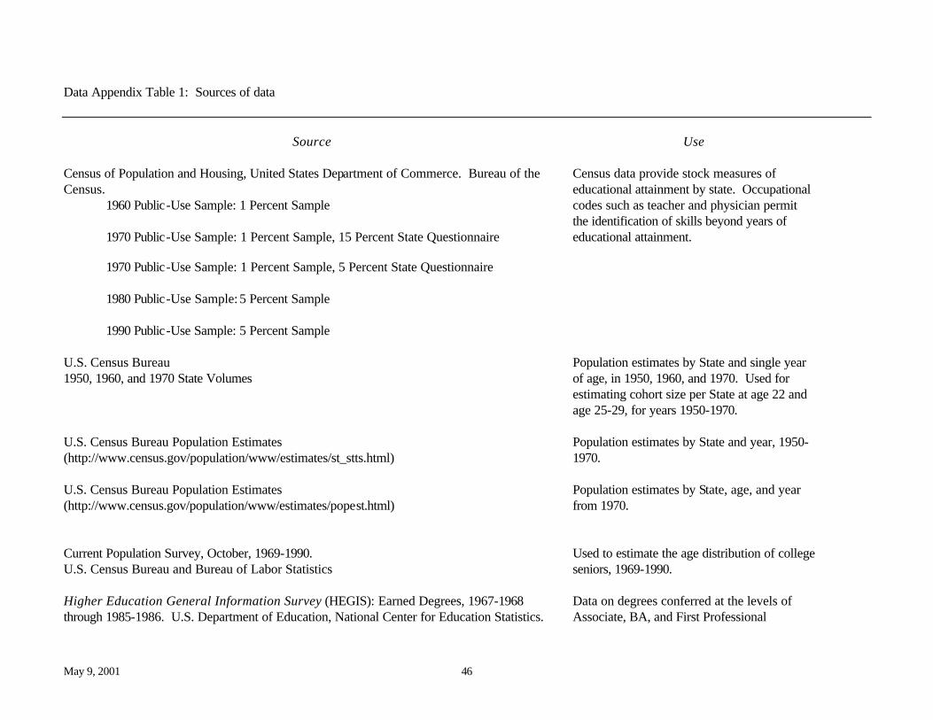
May 9, 2001 46

Data Appendix Table 1: Sources of data

Source

Use

Census of Population and Housing, United States Department of Commerce. Bureau of the Census.

1960 Public-Use Sample: 1 Percent Sample 1970 Public-Use Sample: 1 Percent Sample, 15 Percent State Questionnaire

1970 Public-Use Sample: 1 Percent Sample, 5 Percent State Questionnaire 1980 Public-Use Sample: 5 Percent Sample 1990 Public-Use Sample: 5 Percent Sample

Census data provide stock measures of educational attainment by state. Occupational codes such as teacher and physician permit the identification of skills beyond years of educational attainment.

U.S. Census Bureau 1950, 1960, and 1970 State Volumes U.S. Census Bureau Population Estimates (http://www.census.gov/population/www/estimates/st_stts.html) U.S. Census Bureau Population Estimates (http://www.census.gov/population/www/estimates/popest.html)

Population estimates by State and single year of age, in 1950, 1960, and 1970. Used for estimating cohort size per State at age 22 and age 25-29, for years 1950-1970. Population estimates by State and year, 1950-1970. Population estimates by State, age, and year from 1970.

Current Population Survey, October, 1969-1990. U.S. Census Bureau and Bureau of Labor Statistics

Used to estimate the age distribution of college seniors, 1969-1990.

Higher Education General Information Survey (HEGIS): Earned Degrees, 1967-1968 through 1985-1986. U.S. Department of Education, National Center for Education Statistics.

Data on degrees conferred at the levels of Associate, BA, and First Professional

May 9, 2001 47

Integrated Postsecondary Education Data System (IPEDS): Earned Degrees, 1986-1987 to present. U.S. Department of Education, National Center for Education Statistics. “Earned Degrees Conferred,” Department of Education annual, 1950-1966. National Survey of College Graduates, 1993, National Science Foundation. Physician Professional Data, 1980 and 1991 year-end files, American Medical Association.

collected annually through institutional surveys conducted by the Department of Education. Data contain detailed information on field of study. For a nationally representative sample of college graduates in 1990, the survey contains data on age in 1990 and year of degrees earned. Used for estimating the distribution of age at degree for Engineering BA degrees. Data contain information on date of birth, medical school, and current state of residence for physicians practicing in the U.S. We use these data to construct stocks and flows by State and birth cohort.

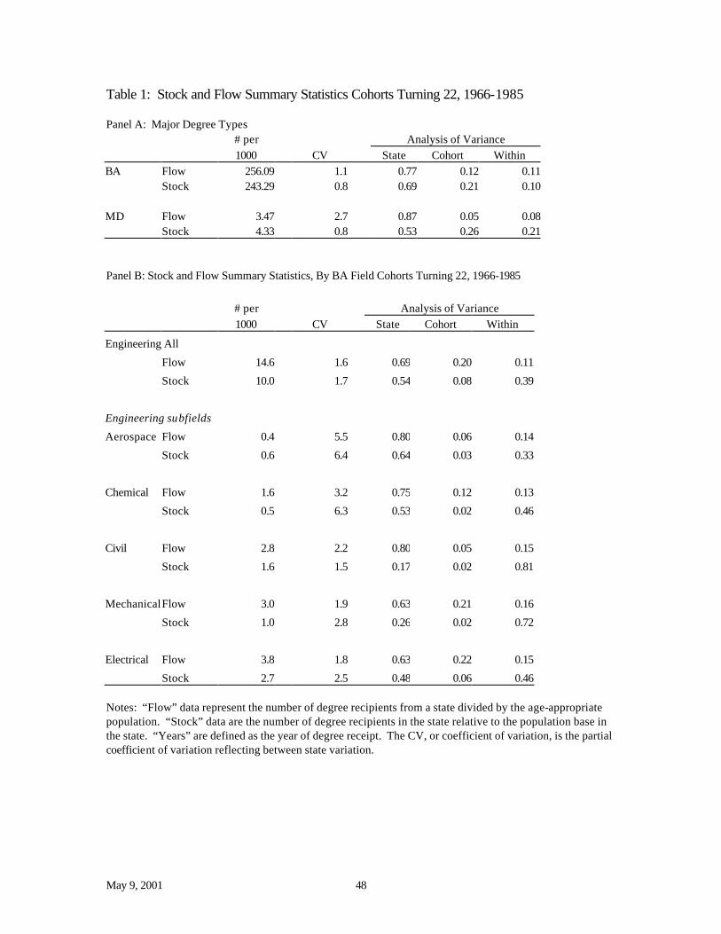
May 9, 2001 48

Table 1: Stock and Flow Summary Statistics Cohorts Turning 22, 1966-1985 Panel A: Major Degree Types # per Analysis of Variance 1000 CV State Cohort Within BA Flow 256.09 1.1 0.77 0.12 0.11 Stock 243.29 0.8 0.69 0.21 0.10 MD Flow 3.47 2.7 0.87 0.05 0.08 Stock 4.33 0.8 0.53 0.26 0.21 Panel B: Stock and Flow Summary Statistics, By BA Field Cohorts Turning 22, 1966-1985

# per Analysis of Variance 1000 CV State Cohort Within

Engineering All

Flow 14.6 1.6 0.69 0.20 0.11

Stock 10.0 1.7 0.54 0.08 0.39

Engineering subfields

Aerospace Flow 0.4 5.5 0.80 0.06 0.14

Stock 0.6 6.4 0.64 0.03 0.33

Chemical Flow 1.6 3.2 0.75 0.12 0.13

Stock 0.5 6.3 0.53 0.02 0.46

Civil Flow 2.8 2.2 0.80 0.05 0.15

Stock 1.6 1.5 0.17 0.02 0.81

Mechanical Flow 3.0 1.9 0.63 0.21 0.16

Stock 1.0 2.8 0.26 0.02 0.72

Electrical Flow 3.8 1.8 0.63 0.22 0.15

Stock 2.7 2.5 0.48 0.06 0.46 Notes: “Flow” data represent the number of degree recipients from a state divided by the age-appropriate population. “Stock” data are the number of degree recipients in the state relative to the population base in the state. “Years” are defined as the year of degree receipt. The CV, or coefficient of variation, is the partial coefficient of variation reflecting between state variation.

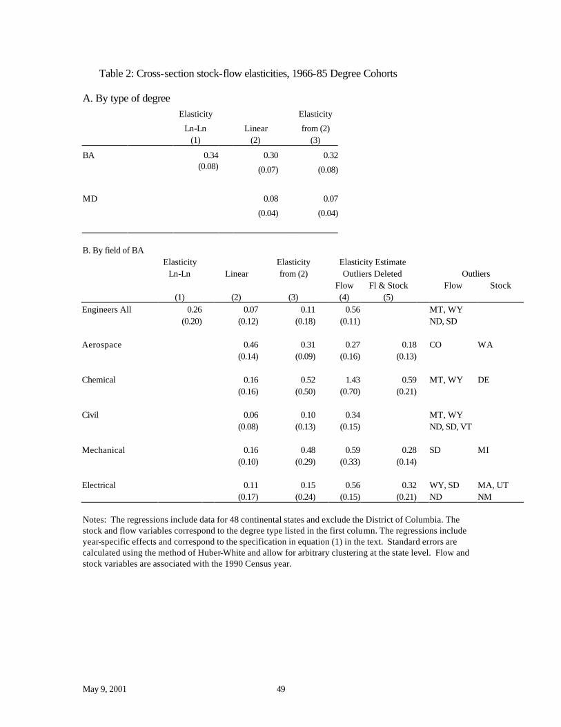
May 9, 2001 49

Table 2: Cross-section stock-flow elasticities, 1966-85 Degree Cohorts

A. By type of degree Elasticity Elasticity

Ln-Ln Linear from (2) (1) (2) (3)

BA 0.34 0.30 0.32

(0.08) (0.07) (0.08)

MD 0.08 0.07

(0.04) (0.04)

B. By field of BA Elasticity Elasticity Elasticity Estimate Ln-Ln Linear from (2) Outliers Deleted Outliers

Flow Fl & Stock Flow Stock (1) (2) (3) (4) (5) Engineers All 0.26 0.07 0.11 0.56 MT, WY (0.20) (0.12) (0.18) (0.11) ND, SD Aerospace 0.46 0.31 0.27 0.18 CO WA (0.14) (0.09) (0.16) (0.13) Chemical 0.16 0.52 1.43 0.59 MT, WY DE (0.16) (0.50) (0.70) (0.21) Civil 0.06 0.10 0.34 MT, WY (0.08) (0.13) (0.15) ND, SD, VT Mechanical 0.16 0.48 0.59 0.28 SD MI (0.10) (0.29) (0.33) (0.14) Electrical 0.11 0.15 0.56 0.32 WY, SD MA, UT (0.17) (0.24) (0.15) (0.21) ND NM Notes: The regressions include data for 48 continental states and exclude the District of Columbia. The stock and flow variables correspond to the degree type listed in the first column. The regressions include year-specific effects and correspond to the specification in equation (1) in the text. Standard errors are calculated using the method of Huber-White and allow for arbitrary clustering at the state level. Flow and stock variables are associated with the 1990 Census year.

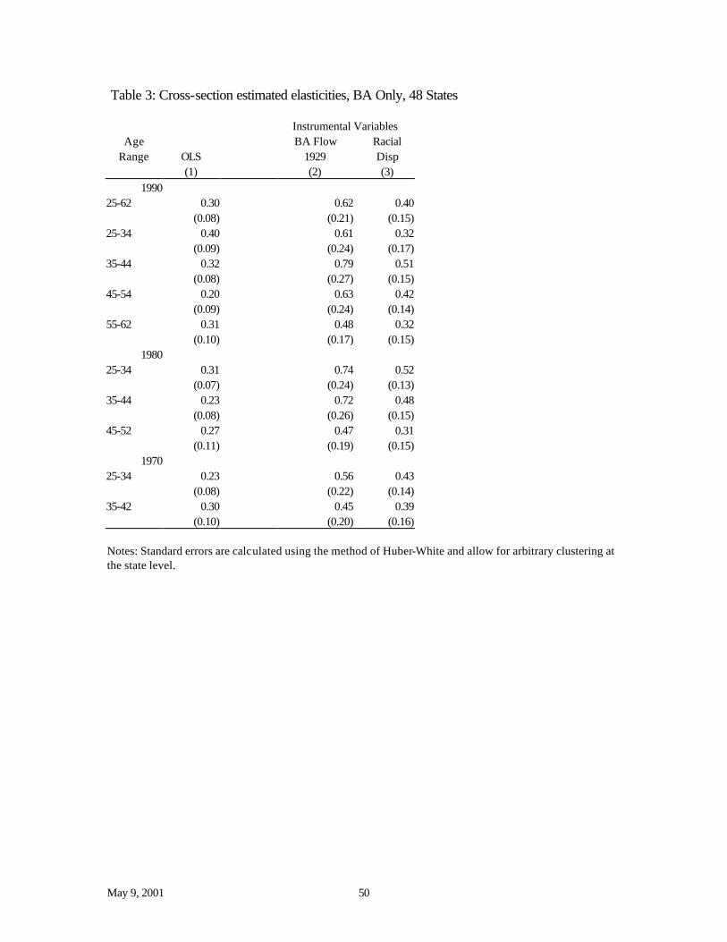
May 9, 2001 50

Table 3: Cross-section estimated elasticities, BA Only, 48 States Instrumental Variables

Age BA Flow Racial Range OLS 1929 Disp

(1) (2) (3) 1990

25-62 0.30 0.62 0.40 (0.08) (0.21) (0.15) 25-34 0.40 0.61 0.32 (0.09) (0.24) (0.17) 35-44 0.32 0.79 0.51 (0.08) (0.27) (0.15) 45-54 0.20 0.63 0.42 (0.09) (0.24) (0.14) 55-62 0.31 0.48 0.32 (0.10) (0.17) (0.15)

1980 25-34 0.31 0.74 0.52 (0.07) (0.24) (0.13) 35-44 0.23 0.72 0.48 (0.08) (0.26) (0.15) 45-52 0.27 0.47 0.31 (0.11) (0.19) (0.15)

1970 25-34 0.23 0.56 0.43 (0.08) (0.22) (0.14) 35-42 0.30 0.45 0.39 (0.10) (0.20) (0.16) Notes: Standard errors are calculated using the method of Huber-White and allow for arbitrary clustering at the state level.

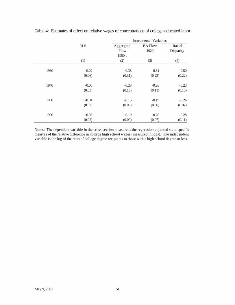
May 9, 2001 51

Table 4: Estimates of effect on relative wages of concentrations of college-educated labor

Instrumental Variables OLS Aggregate BA Flow Racial Flow 1929 Disparity

1950-t (1) (2) (3) (4)

1960 -0.02 -0.38 -0.31 -0.50

(0.06) (0.31) (0.23) (0.22)

1970 -0.06 -0.28 -0.26 -0.23 (0.03) (0.15) (0.11) (0.10)

1980 -0.04 -0.16 -0.19 -0.26 (0.02) (0.08) (0.06) (0.07)

1990 -0.03 -0.19 -0.20 -0.28 (0.02) (0.09) (0.07) (0.11)

Notes: The dependent variable in the cross-section measure is the regression-adjusted state-specific measure of the relative difference in college high school wages (measured in logs). The independent variable is the log of the ratio of college degree recipients to those with a high school degree or less.

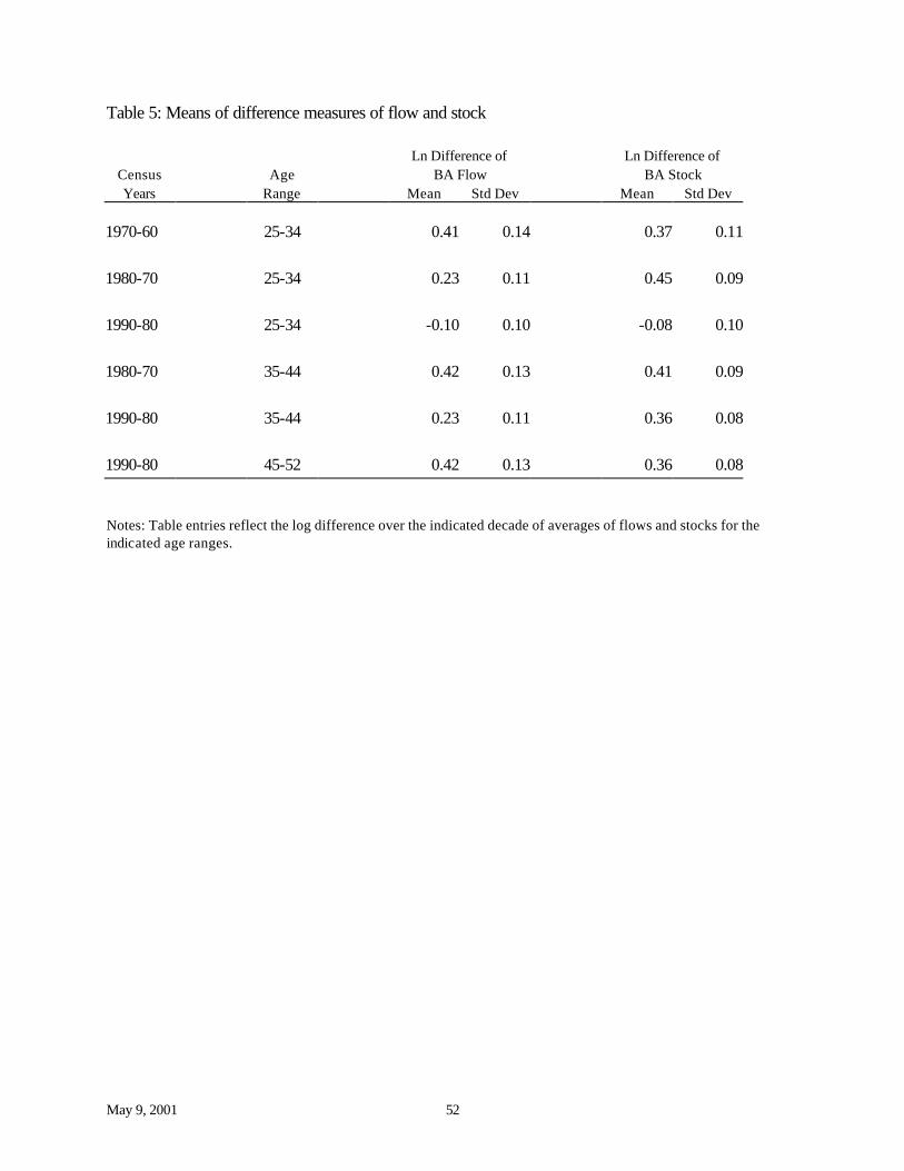
May 9, 2001 52

Table 5: Means of difference measures of flow and stock Ln Difference of Ln Difference of

Census Age BA Flow BA Stock Years Range Mean Std Dev Mean Std Dev

1970-60 25-34 0.41 0.14 0.37 0.11

1980-70 25-34 0.23 0.11 0.45 0.09

1990-80 25-34 -0.10 0.10 -0.08 0.10

1980-70 35-44 0.42 0.13 0.41 0.09

1990-80 35-44 0.23 0.11 0.36 0.08

1990-80 45-52 0.42 0.13 0.36 0.08 Notes: Table entries reflect the log difference over the indicated decade of averages of flows and stocks for the indicated age ranges.

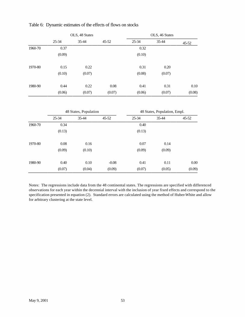
May 9, 2001 53

Table 6: Dynamic estimates of the effects of flows on stocks

OLS, 48 States OLS, 46 States

25-34 35-44 45-52 25-34 35-44 45-52 1960-70 0.37 0.32

(0.09) (0.10)

1970-80 0.15 0.22 0.31 0.20

(0.10) (0.07) (0.08) (0.07)

1980-90 0.44 0.22 0.08 0.41 0.31 0.10

(0.06) (0.07) (0.07) (0.06) (0.07) (0.08)

48 States, Population 48 States, Population, Empl.

25-34 35-44 45-52 25-34 35-44 45-52

1960-70 0.34 0.40

(0.13) (0.13)

1970-80 0.08 0.16 0.07 0.14

(0.09) (0.10) (0.09) (0.09)

1980-90 0.40 0.10 -0.08 0.41 0.11 0.00

(0.07) (0.04) (0.09) (0.07) (0.05) (0.09)

Notes: The regressions include data from the 48 continental states. The regressions are specified with differenced observations for each year within the decennial interval with the inclusion of year fixed effects and correspond to the specification presented in equation (2). Standard errors are calculated using the method of Huber-White and allow for arbitrary clustering at the state level.

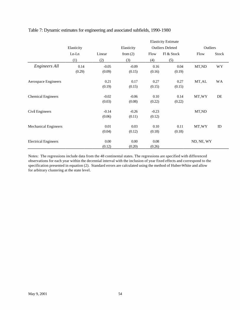
May 9, 2001 54

Table 7: Dynamic estimates for engineering and associated subfields, 1990-1980

Elasticity Estimate

Elasticity Elasticity Outliers Deleted Outliers

Ln-Ln Linear from (2) Flow Fl & Stock Flow Stock

(1) (2) (3) (4) (5)

Engineers All 0.14 -0.05 -0.09 0.16 0.04 MT,ND WY (0.29) (0.09) (0.15) (0.16) (0.19) Aerospace Engineers 0.21 0.17 0.27 0.27 MT,AL WA (0.19) (0.15) (0.15) (0.15) Chemical Engineers -0.02 -0.06 0.10 0.14 MT,WY DE (0.03) (0.08) (0.22) (0.22) Civil Engineers -0.14 -0.26 -0.23 MT,ND (0.06) (0.11) (0.12) Mechanical Engineers 0.01 0.03 0.10 0.11 MT,WY ID (0.04) (0.12) (0.18) (0.18) Electrical Engineers 0.00 0.00 0.08 ND, NE, WY (0.12) (0.20) (0.26) Notes: The regressions include data from the 48 continental states. The regressions are specified with differenced observations for each year within the decennial interval with the inclusion of year fixed effects and correspond to the specification presented in equation (2). Standard errors are calculated using the method of Huber-White and allow for arbitrary clustering at the state level.

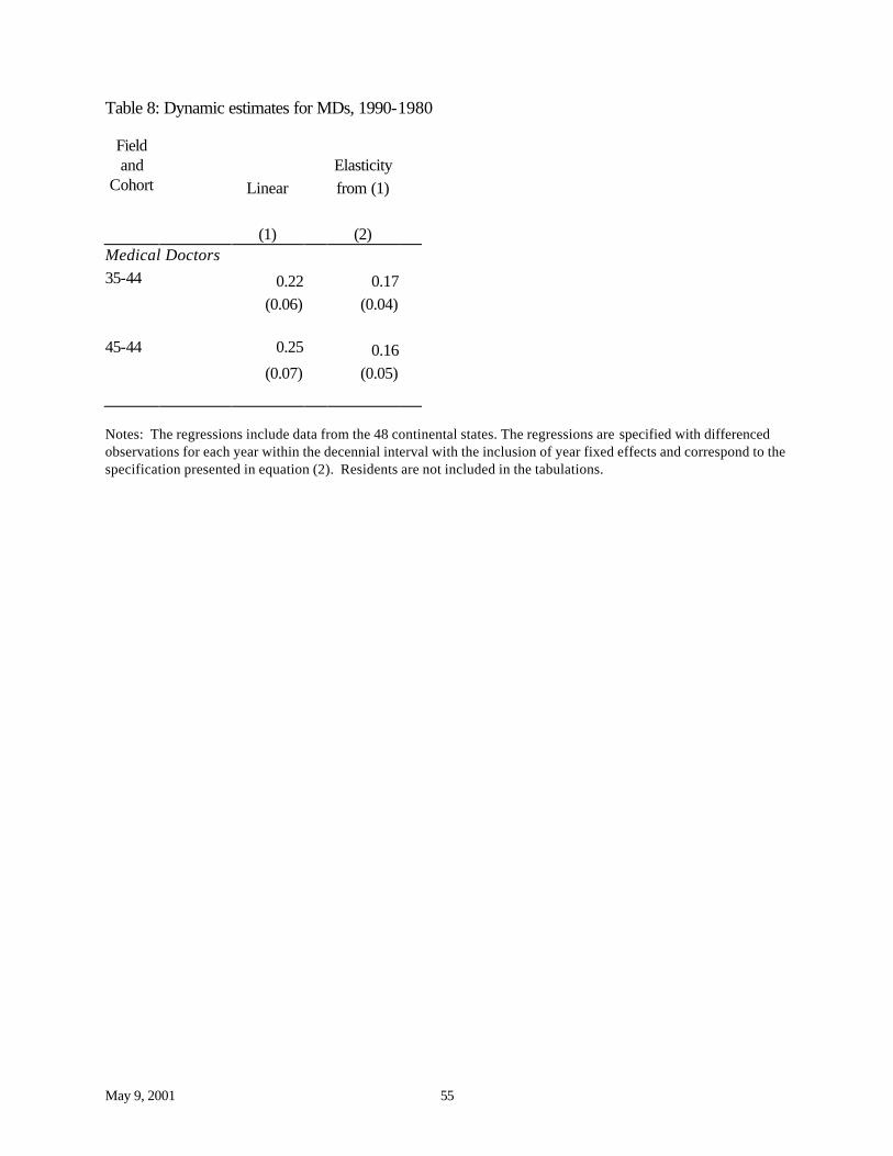
May 9, 2001 55

Table 8: Dynamic estimates for MDs, 1990-1980

Field and Elasticity

Cohort Linear from (1) (1) (2)

Medical Doctors 35-44 0.22 0.17 (0.06) (0.04) 45-44 0.25 0.16 (0.07) (0.05)

Notes: The regressions include data from the 48 continental states. The regressions are specified with differenced observations for each year within the decennial interval with the inclusion of year fixed effects and correspond to the specification presented in equation (2). Residents are not included in the tabulations.

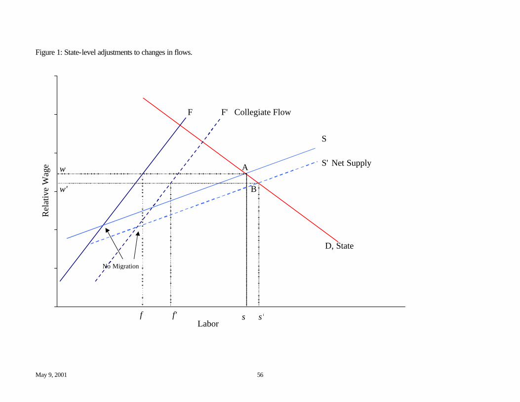
May 9, 2001 56

Figure 1: State-level adjustments to changes in flows.

Labor

Rel

ativ

e W

age

D, State

S

S' Net SupplyA

B

No Migration

F F' Collegiate Flow

w

w'

f f' s s'

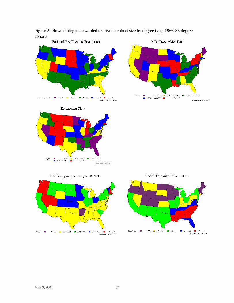
May 9, 2001 57

Figure 2: Flows of degrees awarded relative to cohort size by degree type, 1966-85 degree cohorts

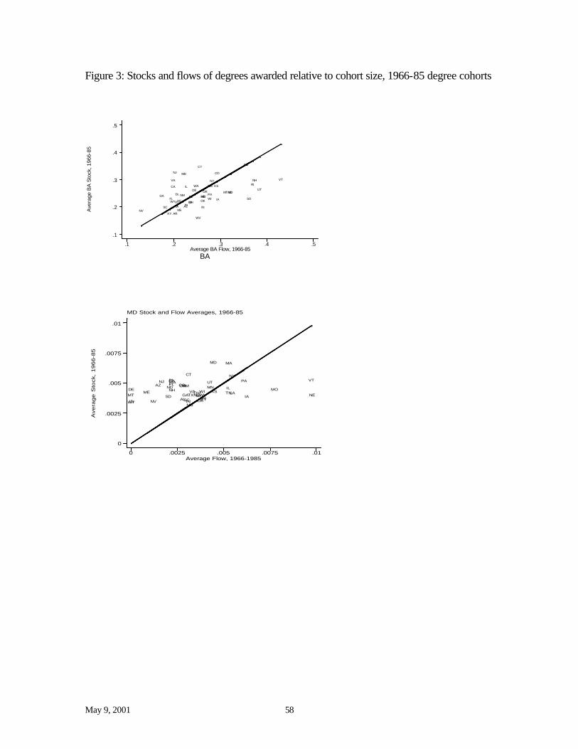
May 9, 2001 58

Figure 3: Stocks and flows of degrees awarded relative to cohort size, 1966-85 degree cohorts

Ave

rage

BA

Sto

ck, 1

966-

85

BAAverage BA Flow, 1966-85

.1 .2 .3 .4 .5

.1

.2

.3

.4

.5

AL

AR

AZ

CA

CO

CT

DE

FLGA

IAID

IL

IN

KS

KY

LA

MA

MD

ME

MI

MN

MO

MS

MT

NC

NDNE

NH

NJ

NM

NV

NY

OH OK

ORPA

RI

SC

SD

TN

TX

UT

VA VT

WA

WI

WV

WY

MD Stock and Flow Averages, 1966-85

A

vera

ge

Sto

ck,

19

66

-85

Average Flow, 1966-19850 .0025 .005 .0075 .01

0

.0025

.005

.0075

.01

AL

AZ

AR

CACO

CT

DEFL

GA

ID

IL

INIA

KS

KY

LAME

MD MA

MI

MN

MS

MO

MT NE

NV

NH

NJNM

NY

NC

ND

OH

OK

ORPARI

SCSD

TNTX

UT VT

VA

WA

WVWI

WY

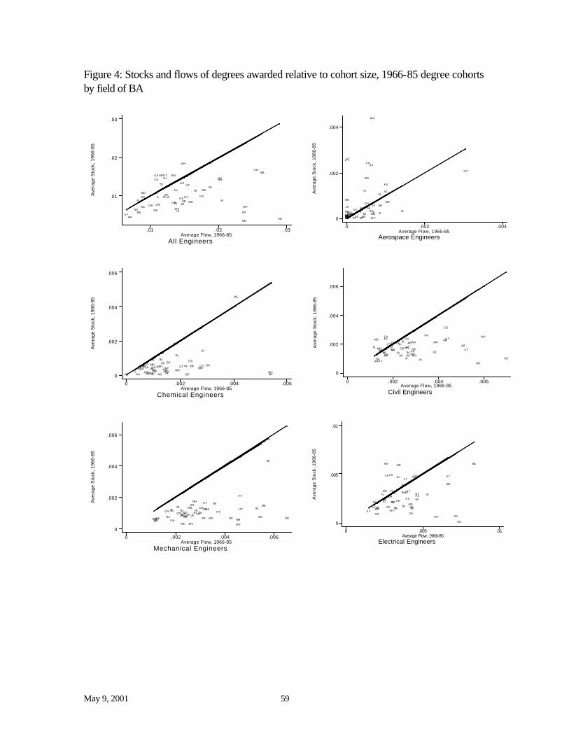
May 9, 2001 59

Figure 4: Stocks and flows of degrees awarded relative to cohort size, 1966-85 degree cohorts by field of BA

A

vera

ge S

tock

, 196

6-85

All EngineersAverage Flow, 1966-85

.01 .02 .03

.01

.02

.03

AL

AR

AZ

CA

CO

CT

DE

FL

GA

IA

IDILIN

KS

KY

LA

MAMD

ME

MI

MN

MO

MS MT

NC

ND

NE

NH

NJ NM

NV

NYOH

OKOR

PA

RI

SC

SD

TN

TX

UTVA

VT

WA

WI

WVWY

A

vera

ge S

tock

, 196

6-85

Aerospace EngineersAverage Flow, 1966-85

0 .002 .004

0

.002

.004

A L

AR

AZCA

CO

CT

DE

FL

GAIA

ID

IL IN

KS

KY

LA MAMD

MEMI MN

MO

MSMTNCNDNE

NHNJ

NM

NV

NY

OH

OK

ORPA

RISCSD

TN

TX

UT

VA

VT

WA

WIWV

WY

A

vera

ge S

tock

, 196

6-85

Chemical EngineersAverage Flow, 1966-85

0 .002 .004 .006

0

.002

.004

.006

AL

AR AZCA

COCT

DE

FLGA

IAID

ILIN

KSKY

LA

MAMD

ME

MIMN

MOMSMT

NC

NDNE

NH

NJ

NM

NV

NY

OHOK

OR

PA

RI

SC

SD

TNTX

UTVA

VTWA

WI

WV

WY

A

vera

ge S

tock

, 196

6-85

Civil EngineersAverage Flow, 1966-85

0 .002 .004 .006

0

.002

.004

.006

AL

AR

AZ

CA

CO

CT

DE

FLGA

IA

ID

IL

IN

KS

KY

LA

MAMDME

MI

MN

MOMS

MT

NC

ND

NE

NHNJ

NM

NVNY

OHOK

ORPA

RISC

SD

TN

TXUTVA

VT

WA

WI WV

WY

A

vera

ge S

tock

, 196

6-85

Mechanical EngineersAverage Flow, 1966-85

0 .002 .004 .006

0

.002

.004

.006

AL

AR

AZCACO

CT

DEFL GA

IA

IDIL INKS

KYLA

MA

MDME

MI

MN

MOMS MTNC ND

NE

NH

NJ

NMNV

NY

OH

OKOR PARISC

SD

TNTX

UT

VA

VT

WA

WI

WV WY

A

vera

ge S

tock

, 19

66-8

5

Electrical EngineersAverage Flow, 1966-85

0 .005 .01

0

.005

.01

A L

AR

AZCA CO

CT

DE

FL

GA

IA

ID

IL IN

KS

KYLA

MAMD

ME

MI

MN

MO

MS MT

NC

ND

NE

NH

NJ

NM

NV

NY

OH

OK

OR PA

RI

SC

SD

TN

TX

UTVAVT

WA

WIWV

WY

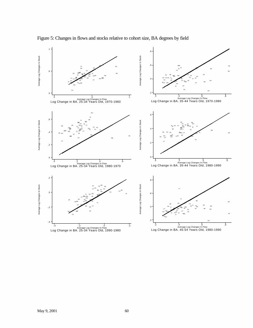
May 9, 2001 60

Figure 5: Changes in flows and stocks relative to cohort size, BA degrees by field

Ave

rage

Log

Cha

nges

In S

tock

Log Change in BA. 25-34 Years Old, 1970-1960Average Log Changes In Flow

0 .5 1

0

.5

1

AL AR

AZ

CACO

CT

DEFL

GA IA

IDIL

IN

KS

KY

LA

MA

MD

ME

MIMNMO

MS

MT

NC

ND

NE

NH

NJNM

NV

NYOH

OK

OR

PARI

SC

SD

TN

TX

UT

VA

VT

WA

WI

WVWY

Ave

rage

Log

Cha

nges

In S

tock


.2 .4 .6 .8

.2

.4

.6

.8

AL

AR

AZ

CACO

CT

DE

FL

GAIA

ID

IL

IN

KS

KY

LA

MAMD

ME

MI

MN

MO

MS

MT

NC

ND

NE

NH

NJ

NM

NV

NY

OH

OK

ORPA

RI

SC

SD

TN

TXUT

VA

VT

WA

WI

WV

WY

Ave

rage

Log

Cha

nges

In S

tock


0 .2 .4 .6

0

.2

.4

.6

AL

AR

AZ

CA

CO CT

DE

FLGA

IA

ID

ILIN

KS

KYLA

MA

MD

ME

MI

MN

MO

MS

MT

NCND

NE

NH

NJ

NM

NV

NYOH

OK

OR

PA

RI

SC

SDTN

TX

UT

VAVT

WA

WI

WV

WY

Ave

rage

Log

Cha

nges

In S

tock


0 .2 .4 .6

0

.2

.4

.6

ALAR

AZ

CA

CO

CT DEFL

GAIA

ID

IL

IN

KS

KY

LA

MA

MD

ME

MIMN

MOMS

MT

NC

ND

NE

NH

NJ NM

NV

NY

OH

OK

OR

PA

RI

SCSD TN

TX

UT

VA

VT

WA

WI

WV

WY

Ave

rage

Log

Cha

nges

In S

tock


-.4 -.2 0 .2

-.4

-.2

0

.2

AL

AR

AZ

CA

CO

CTDE

FL

GA

IA

ID

IL

INKSKY

LA

MAMD

MEMI

MN MO

MS

MT

NC

NDNE

NH

NJ

NM

NV

NY

OH

OK

OR

PA

RISC

SD

TN TX

UT

VA

VT

WA

WI

WV

WY

Ave

rage

Log

Cha

nges

In S

tock


.2 .4 .6 .8

.2

.4

.6

.8

AL

AR

AZ

CACO

CT

DEFL

GAIA

ID

IL

INKS

KY

LA

MA

MD

ME

MIMN

MOMS

MT

NC

ND

NE

NH

NJNM

NV

NY OHOK

OR

PA

RI

SC

SD

TN

TXUT

VA

VT

WA

WI

WV

WY

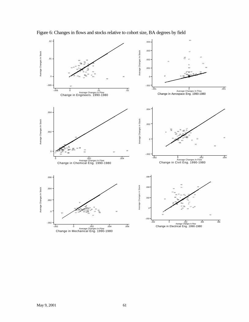
May 9, 2001 61

Figure 6: Changes in flows and stocks relative to cohort size, BA degrees by field

A

vera

ge C

hang

es In

Sto

ck

Change in Aerospace Eng. 1990-1980Average Changes In Flow

-.001 0 .001

-.001

0

.001

.002

.003

.004

AL

AR

AZCA

CO

CT

DE

FL

GA

IA

IDILIN

KSKY

LAMA

MD

ME MI MN

MO

MSMT NCND

NENHNJ

NM

NV

NY OH

OK

OR PARI SCSD

TN

TX

UT

VA

VT

WA

WI WVWY

Ave

rage

Cha

nges

In S

tock

Change in Engineers. 1990-1980Average Changes In Flow

-.005 0 .01 .02

-.005

0

.01

.02

AL

AR

AZ

CA

CO

CT

DE

FLGA

IA

IDIL IN

KSKY

LA

MA

MD

ME

MIMN

MOMS

MT

NC

ND

NE

NH

NJ

NM

NV NY

OH

OK OR

PA

RI SC

SDTN

TX

UT

VA

VT

WA

WI

WV

WY

A

vera

ge C

hang

es In

Sto

ck

Change in Chemical Eng. 1990-1980Average Changes In Flow

0 .002 .004

0

.002

.004

ALARAZ CA COCT

DE

FL

GAIAID IL INKSKY LA

MA

MD

ME

MIMN

MOMSMT

NC

NDNE

NHNJ

NMNV

NY

OH

OK

OR

PA

RI

SC

SD

TN

TXUT

VA

VTWA

WI

WV WY

A

vera

ge C

hang

es In

Sto

ck

Change in Civil Eng. 1990-1980Average Changes In Flow

-.002 0 .002 .004

-.002

0

.002

.004

AL

ARAZ

CA

COCT

DE

FL

GA

IAIDIL IN

KS

KY

LA

MA

MD

ME

MI

MN

MO

MS

MT

NC

ND

NE NHNJ

NM

NV

NYOH

OK

OR

PA

RISC

SDTNTX

UT

VA

VTWA

WIWV

WY

A

vera

ge C

hang

es In

Sto

ck

Change in Mechanical Eng. 1990-1980Average Changes In Flow

-.002 0 .002 .004 .006

-.002

0

.002

.004

.006

ALAR

AZCA

CO

CTDE

FL GAIA

ID

ILIN

KS

KY

LAMA

MD

ME

MI

MN

MOMS

MT

NC

ND

NENHNJNM

NV

NYOH

OK ORPA

RI

SCSD

TNTX UT

VA

VT

WAWI

WVWY

A

vera

ge C

hang

es I

n S

tock

Change in Electrical Eng. 1990-1980Average Changes In Flow

-.002 0 .002 .004 .006

-.002

0

.002

.004

.006

A L

AR

A Z

CA CO

CT

DE

FLGA

IAID

IL

IN

KSKY

LA

MA

MD

ME

MIMN

MOMS

MT

NC

ND

NE

NH

NJNM

NV NYOH

OK

OR

PA

RI

SC

SD

TN

TX

UT

VA

V T

WAWI

WV

WY

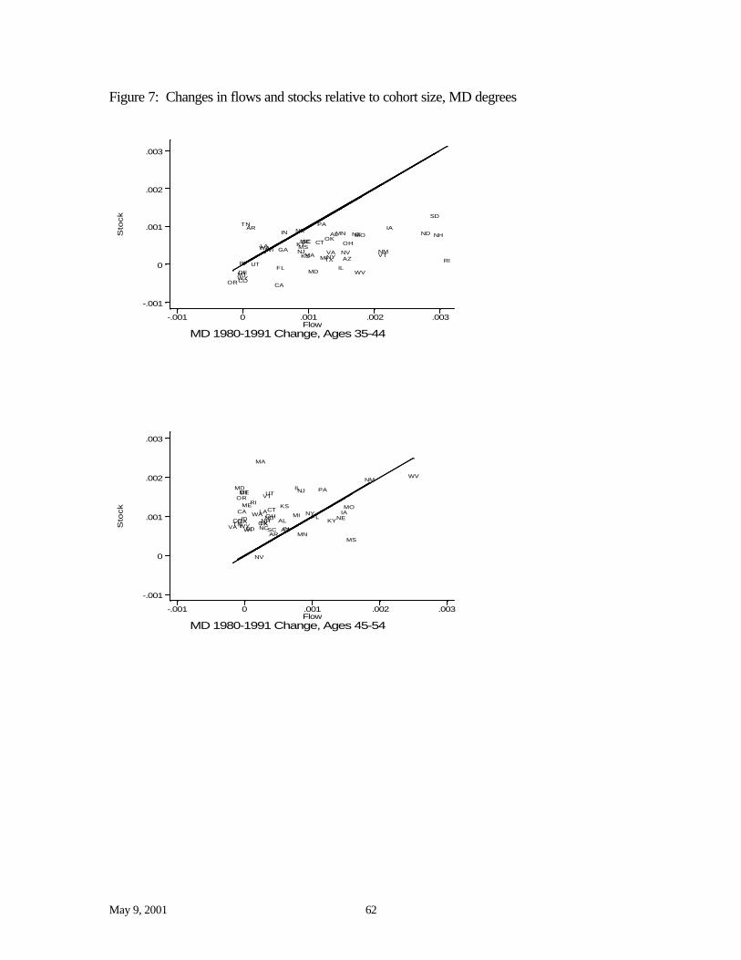
May 9, 2001 62

Figure 7: Changes in flows and stocks relative to cohort size, MD degrees

S

tock

MD 1980-1991 Change, Ages 35-44Flow

-.001 0 .001 .002 .003

-.001

0

.001

.002

.003

AL

AZ

AR

CACO

CT

DEFL

GA

IDIL

INIA

KS

KYLAME

MD

MA MI

MN

MS

MO

MT

NE

NV

NH

NJ NMNY

NC ND

OHOK

OR

PA

RI

SC

SD

TN

TXUT

VTVAWA

WV

WI

WY

S

tock

MD 1980-1991 Change, Ages 45-54Flow

-.001 0 .001 .002 .003

-.001

0

.001

.002

.003

AL

AZAR

CA

CO

CT

DE

FLGAID

IL

IN

IAKS

KY

LAME

MD

MA

MI

MNMS

MO

MT

NE

NV

NH

NJ

NM

NY

NC

NDOHOK

OR

PA

RI

SCSDTN TX

UTVT

VA

WA

WV

WIWY

Trade in university training: cross-state variation in the production and stock of college-educated labor

Documents