Trade Effects of the EU-Mexico Free Trade Agreement Veerle Slootmaekers May 2004 Abstract: The Free Trade Agreement between Mexico and the 15 member countries of the European Union officially entered into force on July 1, 2000. In this empirical study we use a gravity model for import and export flows to quantify the trade effects of the EU-Mexico FTA. Besides the fixed effects approach we apply the instrumental variables estimator developed by Hausman and Taylor (1981). This method - unlike random effects - does not require independence of unobserved and observed characteristics, and allows us to study variables that are fixed over time. Our results indicate that the EU-Mexico FTA had a positive trade creation effect for imports. Moreover there is no evidence for trade diversion; the FTA generated a positive effect on imports with non-members. Finally, other triangular FTAs - a country with which both the US and the EU have signed a FTA - tend to have a negative impact on both imports and exports of the EU and Mexico. Keywords: Gravity Equation, Panel Econometrics, Free Trade Agreement, Mexico, EU. JEL classification: F14, F15, C23 Address: Veerle Slootmaekers Catholic University Leuven Naamsestraat 69 3000 Leuven Belgium E-mail: [email protected]

Welcome message from author
This document is posted to help you gain knowledge. Please leave a comment to let me know what you think about it! Share it to your friends and learn new things together.
Transcript
Trade Effects of the EU-Mexico Free Trade Agreement
Veerle Slootmaekers
May 2004 Abstract: The Free Trade Agreement between Mexico and the 15 member countries of the European Union officially entered into force on July 1, 2000. In this empirical study we use a gravity model for import and export flows to quantify the trade effects of the EU-Mexico FTA. Besides the fixed effects approach we apply the instrumental variables estimator developed by Hausman and Taylor (1981). This method - unlike random effects - does not require independence of unobserved and observed characteristics, and allows us to study variables that are fixed over time. Our results indicate that the EU-Mexico FTA had a positive trade creation effect for imports. Moreover there is no evidence for trade diversion; the FTA generated a positive effect on imports with non-members. Finally, other triangular FTAs - a country with which both the US and the EU have signed a FTA - tend to have a negative impact on both imports and exports of the EU and Mexico. Keywords: Gravity Equation, Panel Econometrics, Free Trade Agreement, Mexico, EU. JEL classification: F14, F15, C23 Address: Veerle Slootmaekers Catholic University Leuven Naamsestraat 69 3000 Leuven Belgium E-mail: [email protected]

1
1 INTRODUCTION
The Free Trade Agreement (FTA) between Mexico and the 15 member countries of
the European Union officially entered into force on the 1st of July 2000. Following the
signature of the EU-Mexico FTA at the European Council in Lisbon on March 23, 2000, tariff
dismantling between the EU and Mexico allowing for preferential access for European and
Mexican exporters into their respective markets began on 1 July 2000. The EU-Mexico FTA
covers a broad spectrum of economic aspects. The comprehensive preferential market access
agreement not only secures liberalized trade in goods and services, it also covers public
procurement, competition, intellectual property rights and dispute resolution. In this paper we
will concentrate on the effects of the agreement on trade between the member countries.
In the first section we give an overview of some essential features of the EU-Mexico
FTA to gain better understanding of the agreement’s effects. Moreover, the influence of the
United States and the North American Free Trade Agreement (NAFTA) on the relationship
between 15 members of the European Union and Mexico is taken into consideration. In the
second section we outline a gravity framework of bilateral trade flows to quantify the trade
effects of the EU-Mexico FTA. Following Bayoumi and Eichengreen (1995) we use a
combination of dummy variables in the gravity model that allows us to separate the trade
creation effects from the trade diversion effects. Moreover, we include an additional dummy
to analyse the impact of triangular free trade agreements on the trade between Mexico and the
European Union. Besides the fixed effects approach we apply the instrumental variables
estimator developed by Hausman and Taylor (1981) to estimate the gravity equation. This
approach permits us to study variables that are fixed over time, while controlling in an
efficient way for the individual effects.
2 THE EU-MEXICO FREE TRADE AGREEMENT
The EU-Mexican FTA liberalised over 96 percent of total trade in goods between the
parties. In industrial goods, Mexico achieved immediate duty-free access to the European
market for 82 percent of its exports, and the remaining 18 percent was fully liberalized by
2003. On the other hand, 60 percent of the export of the European Union could immediately
enter Mexico duty free, while the remaining 40 percent has a maximum tariff level of 5
percent and will be eliminated by 2007. The general structure and provisions of the EU
2
standard protocol were followed in the EU-Mexico FTA. As a result, over 90 percent of the
rules of origin follow the EU harmonized rules, thus simplifying the movement of goods
between Mexico and Europe. Over 95 percent of Mexican exports obtained rules of origin
benefiting national production sectors. Preferential access to the EU for Mexican production
requires that a certain proportion of the product must be produced in Mexico or the EU.1
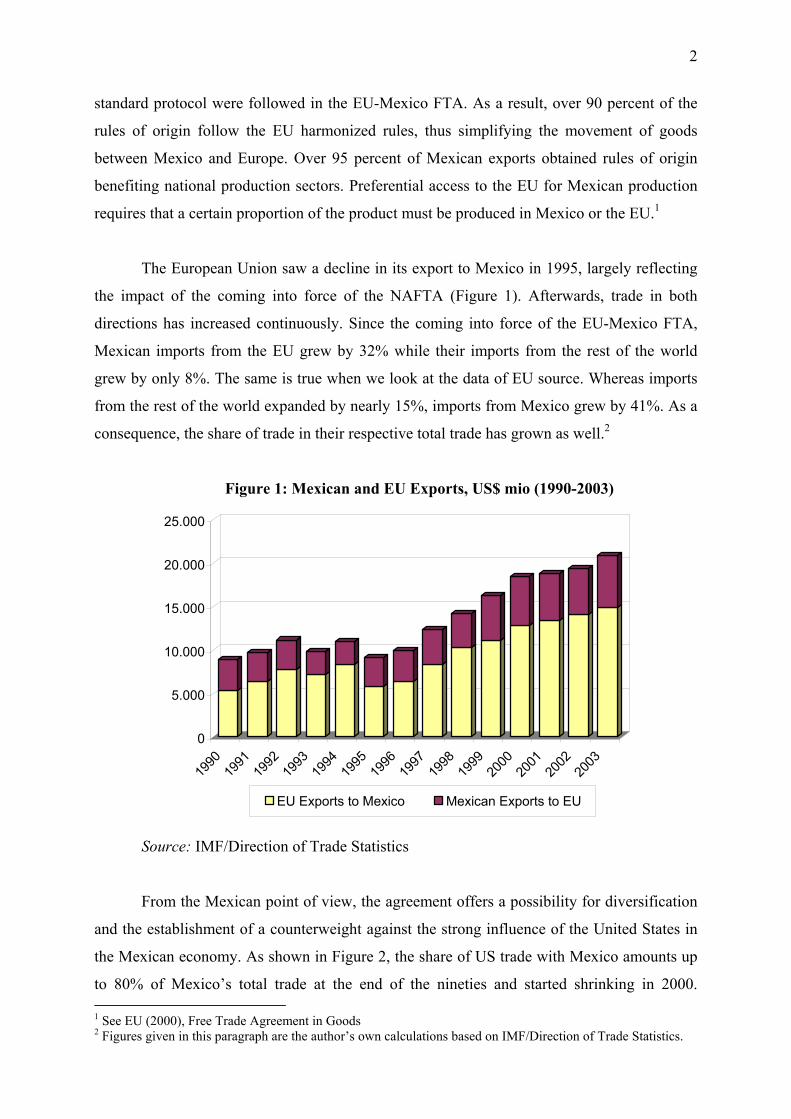
The European Union saw a decline in its export to Mexico in 1995, largely reflecting
the impact of the coming into force of the NAFTA (Figure 1). Afterwards, trade in both
directions has increased continuously. Since the coming into force of the EU-Mexico FTA,
Mexican imports from the EU grew by 32% while their imports from the rest of the world
grew by only 8%. The same is true when we look at the data of EU source. Whereas imports
from the rest of the world expanded by nearly 15%, imports from Mexico grew by 41%. As a
consequence, the share of trade in their respective total trade has grown as well.2
Figure 1: Mexican and EU Exports, US$ mio (1990-2003)
0
5.000
10.000
15.000
20.000
25.000
1990
1991
1992
1993
1994
1995
1996
1997
1998
1999
2000
2001
2002
2003
EU Exports to Mexico Mexican Exports to EU
Source: IMF/Direction of Trade Statistics
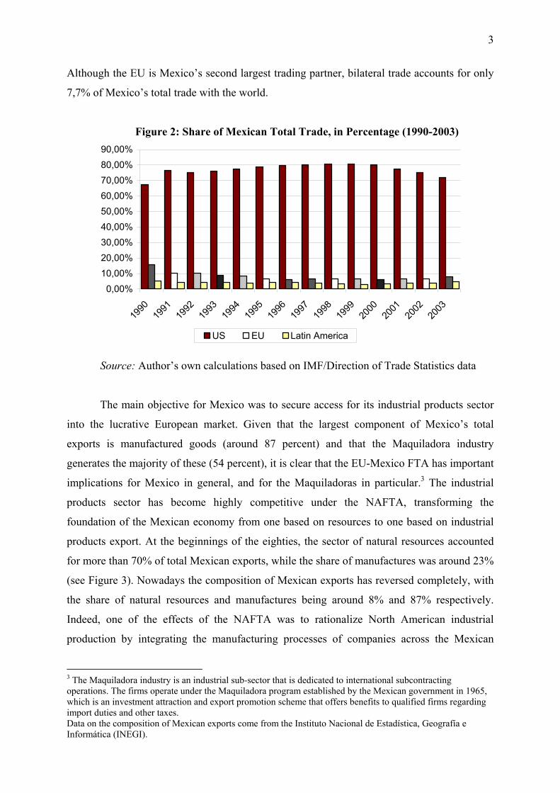
From the Mexican point of view, the agreement offers a possibility for diversification
and the establishment of a counterweight against the strong influence of the United States in
the Mexican economy. As shown in Figure 2, the share of US trade with Mexico amounts up
to 80% of Mexico’s total trade at the end of the nineties and started shrinking in 2000. 1 See EU (2000), Free Trade Agreement in Goods 2 Figures given in this paragraph are the author’s own calculations based on IMF/Direction of Trade Statistics.
3
Although the EU is Mexico’s second largest trading partner, bilateral trade accounts for only
7,7% of Mexico’s total trade with the world.
Figure 2: Share of Mexican Total Trade, in Percentage (1990-2003)
90,00%
80,00%
60,00% 50,00%
40,00%
30,00%
10,00%
0,00%
20,00%
70,00%
1990
1991
1992
1993
1994
1995
1996
1997
1998
1999
2000
2001
2002
2003
US Latin AmericaEU
Source: Author’s own calculations based on IMF/Direction of Trade Statistics data
The main objective for Mexico was to secure access for its industrial products sector
into the lucrative European market. Given that the largest component of Mexico’s total
exports is manufactured goods (around 87 percent) and that the Maquiladora industry
generates the majority of these (54 percent), it is clear that the EU-Mexico FTA has important
implications for Mexico in general, and for the Maquiladoras in particular.3 The industrial
products sector has become highly competitive under the NAFTA, transforming the
foundation of the Mexican economy from one based on resources to one based on industrial
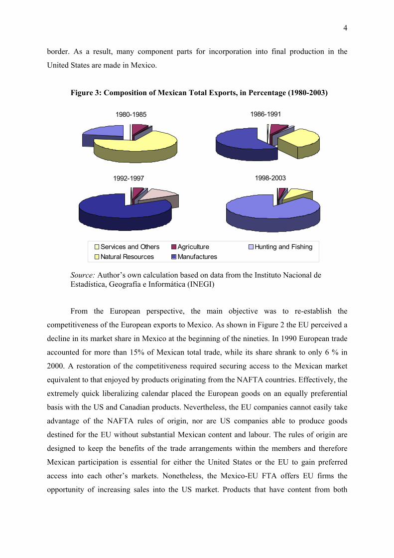
products export. At the beginnings of the eighties, the sector of natural resources accounted
for more than 70% of total Mexican exports, while the share of manufactures was around 23%
(see Figure 3). Nowadays the composition of Mexican exports has reversed completely, with
the share of natural resources and manufactures being around 8% and 87% respectively.
Indeed, one of the effects of the NAFTA was to rationalize North American industrial
production by integrating the manufacturing processes of companies across the Mexican
3 The Maquiladora industry is an industrial sub-sector that is dedicated to international subcontracting operations. The firms operate under the Maquiladora program established by the Mexican government in 1965, which is an investment attraction and export promotion scheme that offers benefits to qualified firms regarding import duties and other taxes. Data on the composition of Mexican exports come from the Instituto Nacional de Estadística, Geografía e Informática (INEGI).
4
border. As a result, many component parts for incorporation into final production in the
United States are made in Mexico.
Figure 3: Composition of Mexican Total Exports, in Percentage (1980-2003)
1998-2003
Services and Others Agriculture Hunting and Fishing
1980-1985 1986-1991
1992-1997
Natural Resources Manufactures
Source: Author’s own calculation based on data from the Instituto Nacional de Estadística, Geografía e Informática (INEGI)
From the European perspective, the main objective was to re-establish the
competitiveness of the European exports to Mexico. As shown in Figure 2 the EU perceived a
decline in its market share in Mexico at the beginning of the nineties. In 1990 European trade
accounted for more than 15% of Mexican total trade, while its share shrank to only 6 % in
2000. A restoration of the competitiveness required securing access to the Mexican market
equivalent to that enjoyed by products originating from the NAFTA countries. Effectively, the
extremely quick liberalizing calendar placed the European goods on an equally preferential
basis with the US and Canadian products. Nevertheless, the EU companies cannot easily take
advantage of the NAFTA rules of origin, nor are US companies able to produce goods
destined for the EU without substantial Mexican content and labour. The rules of origin are
designed to keep the benefits of the trade arrangements within the members and therefore
Mexican participation is essential for either the United States or the EU to gain preferred
access into each other’s markets. Nonetheless, the Mexico-EU FTA offers EU firms the
opportunity of increasing sales into the US market. Products that have content from both

5
Mexico and the European Union have a tariff advantage compared with products either
coming directly from the EU of from other parts of the world.
3 EMPIRICAL EVALUATION
3.1 The Standard Gravity Model
To identify the effects of the FTA it is important to disentangle the effects of regional
integration from other changes in the economy. A standard way to control for these other
effects is to run a gravity model, and see whether the estimated relationships change as a
consequence of implementing the FTA.4 The ‘standard’ gravity model estimates bilateral
trade between countries and explains trade as a function of their GDPs, populations, the
distance between them, and additional factors such as sharing land border and common
language. Furthermore a dummy is included to capture the integration effect of the FTA. A
positive and significant coefficient on the FTA dummy is taken as evidence that during these
years the countries traded more than would be suggested by other factors.
The specification of the standard gravity equation takes the following form:
tijiijijtjtitiijt DDPYYT µβββββα ++++++= lnlnlnlnlnln 54321
where all variables are expressed in logs:
=ijtT Total bilateral trade (sum of imports and exports) between countries i and j at
time t, with i ≠ j (Source: IMF/Direction of Trade Statistics);
=itY Gross domestic product of country i at time t (IMF, expanded with WB/WDI
data);
=ijtP Joint population of country i and country j at time t (IMF, expanded with
WB/WDI data);
4 Theoretical foundations of the gravity model are provided by Deardorff (1984), Helpman and Krugman (1985), and Helpman (1987). For a comprehensive overview of the empirical literature see Frankel (1997), and Harrigan (2002).

6
=ijD Distance between country i and country j (Geodesic distances from Centre
d'Etudes Prospectives et d'Informations Internationales, CEPII);5
=iD Remoteness, which is the average distance between country i and its exports
markets in other countries, weighted by the GDP;
=ijtµ Residual term;
Trade is viewed as being positively affected by the economic mass of trading partners
(larger economies are likely to trade more), and negatively by population. A larger population
is expected to reduce trade orientation by increasing the size of the domestic market and
making economic activity more inwardly oriented. Distance between trading partners is used
as a proxy for the cost of international transaction of goods and services and is expected to
affect trade negatively. In addition to the absolute level of bilateral distance we include a
measure of the remoteness of a country. An exporter’s remoteness is defined as its average
distance from its trading partners, using the partners’ GDP as weights. The hypothesis is that
the bilateral distance between two countries relative to the distances to their other trading
partners has a positive effect on bilateral trade. For example, the distance between New
Zealand and Australia is the same as the distance between France and Turkey. While France
and Turkey have lots of other natural trading partners close by, New Zealand and Australia do
not. We might thus expect the latter country pair, who have less alternatives, to trade more
with each other, ceteris paribus, than France and Turkey.
Besides distance there are other factors influencing the cost of doing business at a
distance. Linneman (1966) called this “physic distance” or “cultural unfamiliarity”, which
refers to the lack of familiarity with another country’s laws, institutions, habits, and
languages. Hence we include several dummies to capture these additional features of a
country pair.6
=ijL Dummy that equals 1 if country i and country j have the same language, zero
otherwise;
=ijA Dummy that equals 1 if country i and country j have a common border, zero
otherwise;
5 The geodesic distances are calculated following the great circle formula, which uses latitudes and longitudes of the most important cities/agglomerations (in terms of population). 6 The two dummies indicating the adjacent borders and a common language between countries are obtained from the Centre d'Etudes Prospectives et d'Informations Internationales, CEPII.

7
Since linguistic affinity and shared borders tend to reduce the cultural distance and
therefore encourage bilateral trade, we expect 6β and 7β to be positive. The new equation
becomes:
tijijijiijijtjtitiijt ALDDPYYT µβββββββα ++++++++= 7654321 lnlnlnlnlnln
Following Bayoumi and Eichengreen (1995) we include extra variables to capture
third-country effects. Besides the real exchange rate vis-à-vis the US dollar ( ), as used by
Bayoumi and Eichengreen (1995), we add the GDP of the US (Y ) as well. Since the
Mexican economy is highly dependent on the US economy, changes in the GDP of the US
might have important effects on Mexican trade. Omitting these two extra variables would lead
to an omitted-variables bias in our gravity equation. The standard gravity model assumes that
bilateral trade depends only on economic conditions in the two countries considered. In
practice, however, bilateral trade also depends on competitiveness relative to other countries
and markets.
itER
USt
In order to capture the trade effect of the EU-Mexico FTA we extend the standard
gravity equation and add a dummy that equals one if both countries belong to the EU-Mexico
FTA and zero otherwise. The estimated efficient of this dummy variable is the sum of the
trade-creation and the trade-diversion effects of the EU-Mexico FTA. A positive coefficient
indicates that the FTA tends to generate more trade to its members.
tijtit
UStijijiijijtjtitiijt
EUMexFTAERYALDDPYYT
µββ
ββββββββα
++
+++++++++=
109
87654321 lnlnlnlnlnln
3.2 Empirical Results
The database used in estimating the gravity model contains panel data for 179
countries over the period 1980-2003. We use panel data to take into account the critic of
Mátyás (1997). He argues that the traditional cross-section approach is affected by a severe
problem of misspecification. The most natural representation of bilateral trade flows is a
three-way specification and eliminating one of the three dimensions (e.g. time) ignores the
presence of exporter and importer effects. Egger (2002) adds to this argument that a panel

8
framework the most appropriate methodology is for disentangling time-invariant and country
specific effects.
We estimate the model with fixed effects (FE) and with random effects (RE). Whereas
the FE model is always consistent in the absence of endogeneity or errors in variables, the RE
model is only consistent if the individual effects are uncorrelated with all other explanatory
variables. In that case, RE estimators have the advantage to be more efficient than FE
estimators. If these conditions do not hold, only the FE approach is consistent since it cleans
out all the time-invariant effects ( iα ). The Hausman (1978) specification test is used to test
for correlation between the whole set of explanatory variables and the country-specific
effects. As shown in table 1, the null hypothesis of zero correlation is rejected in all
specification tried, which indicates that the RE estimates are biased.
The results of our gravity estimation are reported in table 1. Dhar and Panagariya
(1999) argue that using total trade as dependent variable constrains the coefficients for
imports and exports to be equal. Instead they propose to estimate separate equations for
exports and imports. On the other hand, according to Frankel (1997) aggregating imports and
exports influences only slightly the results. Moreover, he argues that it has the advantage to
cancel out the effect of a real appreciation or depreciation on exports and imports and thus
justifies the omission of a term for the real exchange rate. To check the validity of our
estimation results, we compare the estimates of separate equations for imports ( ln ),
exports ( ln ), and aggregate trade ( ln ). As reported in table 1, the difference between
the import elasticity and export elasticity is substantially large. Constraining them to be equal
and using total trade as dependent variable would therefore be inappropriate. Consequently,
for the remaining of the paper the difference in coefficients will be taken into account, and the
results will be discussed for imports and exports separately.
ijtM
ijtX ijtT
Furthermore we include a linear time trend term to control for the observed tendency
that international trade grows over time. The trend term turns out to be statistically significant,
and moreover the results change in important ways. The R-squared of the regressions with
time trend is considerably higher compared to R-squared of the regressions without time
trend, both for exports and imports.

9
Table 1: Gravity Model Estimates, using FE (1980-2003)
Variable ijtTln ijtTln ijtXln ijtXln ijtMln ijtMln
C -15.748*** (1.870)
-79.425*** (5.687)
-13.577*** (2.112)
-105.038***(6.410)
-21.394*** (2.748)
-125.603***(8.348)
itY 0.147*** (0.034)
0.179*** (0.034)
0.053 (0.038)
0.102*** (0.038)
0.359*** (0.049)
0.412*** (0.049)
jtY 0.854*** (0.021)
0.883*** (0.021)
0.836*** (0.024)
0.876*** (0.024)
0.809*** (0.031)
0.856*** (0.031)
ijD dropped dropped dropped dropped dropped dropped
iD 0.000*** (0.000)
-0.000 (0.000)
0.000*** (0.000)
0.000 (0.000)
0.001*** (0.000)
0.000*** (0.000)
ijL dropped dropped dropped dropped dropped dropped
ijA dropped dropped dropped dropped dropped dropped
ijtP -1.040*** (0.141)
-0.859*** (0.142)
-1.691*** (0.159)
-1.437*** (0.160)
-0.683*** (0.207)
-0.392* (0.208)
UStY 0.399*** (0.045)
2.530*** (0.185)
0.727*** (0.051)
3.791*** (0.209)
0.027 (0.067)
3.516*** (0.272)
itER 0.000*** (0.000)
0.000*** (0.000)
0.000** (0.000)
0.000*** (0.000)
0.000*** (0.000)
0.000*** (0.000)
tEUMexFTA 0.009 (0.088)
0.103 (0.088)
-0.076 (0.100)
0.059 (0.100)
0.090 (0.130)
0.244* (0.130)
Trend -0.127*** (0.011) -0.183***
(0.012) -0.208*** (0.016)
Observations 54478 54478 54944 54944 54663 54663 2R 0.2280 0.3714 0.0394 0.1684 0.1457 0.3561
F-statistic 834.68*** 749.87*** 793.39*** 725.76*** 383.06*** 358.13*** Hausman test
2χ 846.78*** 522.48*** 1112.83*** 464.19*** 730.22*** 372.22***
*** Significant at 99% confidence level; ** significant at 95% confidence level; * significant at 90% confidence level.
As reported in table 1, all the coefficients have the expected signs and are statistically
significant, with exception of iD and the FTA dummy for exports.7 Since the explanatory
variables , , and are time-invariant variables, they are wiped out by the FE estimator.
As expected, exports and imports are positively affected by the log of GDP and negatively by
the log of population. Both for exports and imports the GDP of the trading partner seems to
have a relatively larger effect than a country’s own GDP. The estimated coefficients for the
log of GDP are less than one. This indicates that, though trade increases with size, it increases
less than proportionately (ceteris paribus). This reflects that small economies tend to be more
ijD ijL ijA
7 The effect of the FTA dummy on exports and imports will be further elaborated in the next section.
10
dependent on international trade than larger, more diversified economies. The effect of a
country’s remoteness on imports is positive and statistically highly significant, as one would
expect, but is of little economic relevance. The effect on exports is nor statistically significant,
nor economically significant. The same conclusion counts for the effect of the real exchange
rate on exports and imports. Although the coefficient of the real exchange rate is statistically
significant, the effect is practically very small. On the other hand, US GDP influences in a
strong way exports and imports between countries and the coefficient is statistically
significant. When the US GDP increases by 1%, the exports and imports between Mexico and
the EU and their trading partners will increase on average by 3,8% and 3,5% respectively
(ceteris paribus). US GDP turns out to be the most important basic factor in determining trade
flows.
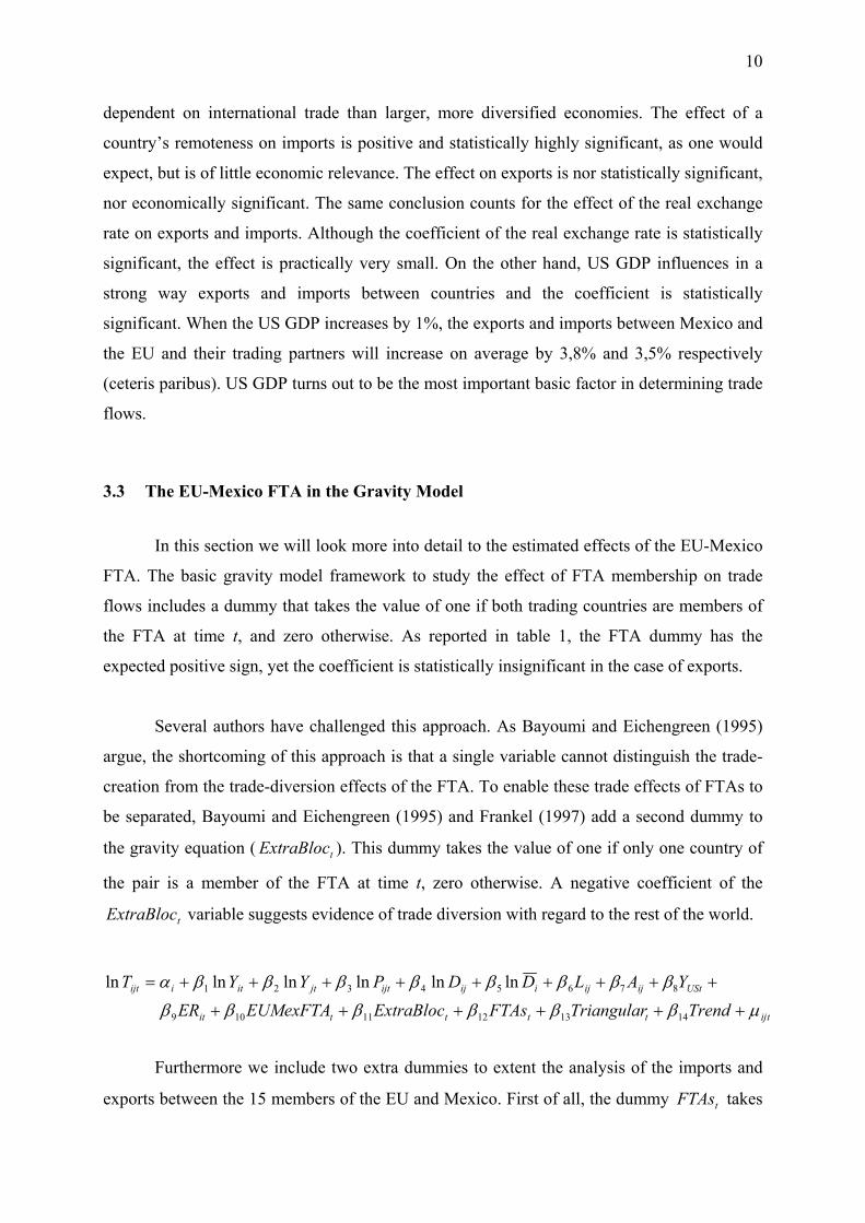
3.3 The EU-Mexico FTA in the Gravity Model
In this section we will look more into detail to the estimated effects of the EU-Mexico
FTA. The basic gravity model framework to study the effect of FTA membership on trade
flows includes a dummy that takes the value of one if both trading countries are members of
the FTA at time t, and zero otherwise. As reported in table 1, the FTA dummy has the
expected positive sign, yet the coefficient is statistically insignificant in the case of exports.
Several authors have challenged this approach. As Bayoumi and Eichengreen (1995)
argue, the shortcoming of this approach is that a single variable cannot distinguish the trade-
creation from the trade-diversion effects of the FTA. To enable these trade effects of FTAs to
be separated, Bayoumi and Eichengreen (1995) and Frankel (1997) add a second dummy to
the gravity equation ( ). This dummy takes the value of one if only one country of
the pair is a member of the FTA at time t, zero otherwise. A negative coefficient of the
variable suggests evidence of trade diversion with regard to the rest of the world.
tExtraBloc
tExtraBloc
tijttttit
UStijijiijijtjtitiijt
TrendTriangularFTAsExtraBlocEUMexFTAERYALDDPYYT
µββββββ
ββββββββα
++++++
+++++++++=
14131211109
87654321 lnlnlnlnlnln
Furthermore we include two extra dummies to extent the analysis of the imports and
exports between the 15 members of the EU and Mexico. First of all, the dummy takes tFTAs
11
the value one if both countries of a country pair belong to a certain free trade agreement or
custom union at time t, zero otherwise.8 This dummy is introduced in the gravity model in
order to capture the global impact of regional integration on trade between Mexico and the
EU and their trading partners. According to the common finding from the regional integration
literature that positive trade effects are associated with regional trade agreements, we expect
the coefficient on to be positive. tFTAs
In addition, we include a second additional dummy (Triangular ), which takes the
value one if both the EU and the US have a FTA with a particular country at time t, zero
otherwise. Gambrill (2002) argues that the trade between the EU and Mexico is characterized
by triangular trade of European goods through Mexico into the US market, as well as a
reverse triangular trade from third parties, such as the US or Asian countries, through Mexico
into the EU market. Moreover, she argues that this trade pattern has been reinforced by the
specific rules of origin defined in the EU-Mexico FTA. For example, on the one hand, goods
subcontracted in Mexico by European Maquiladoras are often exported directly from Mexico
to other countries such as the US. This indicates that the European subcontracting operations
in the Maquiladoras is not ‘outward processing’, in which EU companies assemble goods in
underdeveloped countries and then return them to the European market. On the other hand,
European companies source intermediary goods in Asia and the US, bring them to Mexico,
where they are processed, and export them to the EU. Of course, the rules of origin are
designed to keep the benefits of the trade arrangements within the members, and thus Asian or
US goods assembled in Mexico cannot easily receive the tariff benefits negotiated under the
EU-Mexico FTA. Nevertheless, if the non-originating goods are transformed by more
complex manufacturing processes, the status of originating products can be conferred to the
intermediary goods coming from third countries.
t
9
There is a possibility that the same triangular trade pattern exists for other countries
with which both the US and the EU have signed a FTA, namely Israel and Jordan. On the one
hand, the US signed a FTA with Israel in August 1985 and with Jordan in December 2001.
On the other hand, the FTA between the 15 members of the EU, and Israel and Jordan
officially entered into force in respectively November 2000 and December 2002, which
8 Other forms of integration arrangements, as preferential trading areas or services agreements, are not taken into account. The analysis is concentrated on more profound integration arrangements. 9 Details on the Rules of Origin can be found in EU-Mexico Free Trade Agreement, Trade in Goods, Annex III. Available at: http://www.europa.eu.int/comm/trade/bilateral/mexico/fta.htm

12
means that since these dates the triangular trade pattern is open for Israel and Jordan.10 The
existence of possibility for an alternative triangular trade agreement would reduce the
importance of the triangular trade between the EU and Mexico, since the EU companies have
the possibility to export their goods through Israel or Jordan into the US market. Therefore,
negative coefficient of the dummy Triangular is expected. t
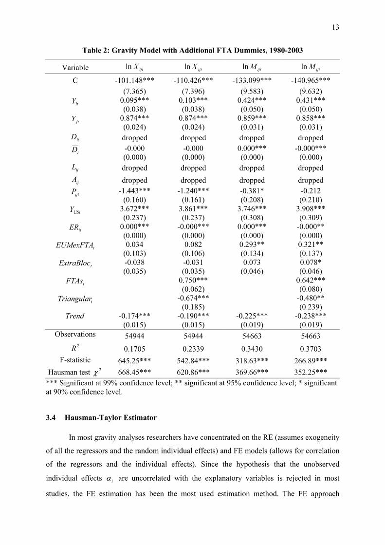
The results of the gravity model with the additional FTA-dummies are reported in
table 2. As we can see, the coefficient of for imports not only becomes bigger in
economic terms, it is now statistically significant at a 95% confidence level. As the dependent
variable is in logarithmic form, this implies that imports of the EU and Mexico are about
37,9% [exp(0,321) – 1 ≈ 0,379] higher than would have been expected by their economic
characteristics and the average behaviour of countries in the sample. In addition, there seems
to be no evidence of trade diversion. The coefficient of has a positive sign and is
statistically significant at a 90% confidence level. This result indicates that membership of the
EU-Mexico FTA did not only significantly expand imports between Mexico and the 15
members of the European Union, but also from the rest of the world. Greater trade with the
rest of the world accompanied the tendency for greater intra-bloc trade, though of a smaller
magnitude, about 8,1% [exp(0,078) – 1 ≈ 0,081]. As shown in table 2, the coefficients of
and for exports have the expected signs, however they are
statistically insignificant.
tEUMexFTA
tExtraBloc
tEUMexFTA tExtraBloc
We now focus on the results of the two additional dummies that were included in the
gravity model. As reported in table 2, both dummies have the expected sign and are
statistically highly significant, for exports as well as for imports. Even when we control for
other effects, being member of a free trade agreement, has a positive effect on the trade of
Mexico and the EU. Moreover, as expected, other triangular trade agreements reduce trade
between Mexico and the EU. This means that the European companies have alternatives,
beside Mexico, to export their goods under preferential access to the US. Imports and exports
are respectively about 38,1% and 49,0% lower than what would have been expected without
the existence of the alternative triangular free trade agreements.
10 See WTO (2000)
13
Table 2: Gravity Model with Additional FTA Dummies, 1980-2003
Variable ijtXln ijtXln ijtMln ijtMln
C -101.148*** (7.365)
-110.426*** (7.396)
-133.099*** (9.583)
-140.965*** (9.632)
itY 0.095*** (0.038)
0.103*** (0.038)
0.424*** (0.050)
0.431*** (0.050)
jtY 0.874*** (0.024)
0.874*** (0.024)
0.859*** (0.031)
0.858*** (0.031)
ijD dropped dropped dropped dropped
iD -0.000 (0.000)
-0.000 (0.000)
0.000*** (0.000)
-0.000*** (0.000)
ijL dropped dropped dropped dropped
ijA dropped dropped dropped dropped
ijtP -1.443*** (0.160)
-1.240*** (0.161)
-0.381* (0.208)
-0.212 (0.210)
UStY 3.672*** (0.237)
3.861*** (0.237)
3.746*** (0.308)
3.908*** (0.309)
itER 0.000*** (0.000)
-0.000*** (0.000)
0.000*** (0.000)
-0.000** (0.000)
tEUMexFTA 0.034 (0.103)
0.082 (0.106)
0.293** (0.134)
0.321** (0.137)
tExtraBloc -0.038 (0.035)
-0.031 (0.035)
0.073 (0.046)
0.078* (0.046)
tFTAs 0.750*** (0.062) 0.642***
(0.080) tTriangular -0.674***
(0.185) -0.480** (0.239)
Trend -0.174*** (0.015)
-0.190*** (0.015)
-0.225*** (0.019)
-0.238*** (0.019)
Observations 54944 54944 54663 54663 2R 0.1705 0.2339 0.3430 0.3703
F-statistic 645.25*** 542.84*** 318.63*** 266.89*** Hausman test 2χ 668.45*** 620.86*** 369.66*** 352.25***
*** Significant at 99% confidence level; ** significant at 95% confidence level; * significant at 90% confidence level.
3.4 Hausman-Taylor Estimator
In most gravity analyses researchers have concentrated on the RE (assumes exogeneity
of all the regressors and the random individual effects) and FE models (allows for correlation
of the regressors and the individual effects). Since the hypothesis that the unobserved
individual effects iα are uncorrelated with the explanatory variables is rejected in most
studies, the FE estimation has been the most used estimation method. The FE approach
14
essentially eliminates the iα from the model by transforming the data into deviations from
their individual means. Unfortunately, all time-invariant variables are eliminated as well by
the transformation, so that these coefficients cannot be estimated. Moreover, under certain
circumstances, the FE estimator is not fully efficient, since it ignores variation across
individuals in the sample. Hence, Hausman and Taylor (1981) provide an alternative that
avoids the ‘all or nothing’ choice between FE and RE. The resulting instrumental variable
estimator explicitly accounts for the fact that some explanatory variables are correlated with
the country-specific effects iα and others not.
,2X it
iα
To describe the general approach, consider a linear model with four groups of
explanatory variables (Hausman and Taylor, 1981)
,221121,10 itiiiitit ZZXY µαγγβββ ++++++=
The Hausman-Taylor estimator (denoted as HT hereafter) assumes that some of the
explanatory variables are correlated with iα , but none with itµ . Their approach is based on
the notion that we can divide the regressors into four categories: time varying ( X ) / time
invariant ( Z ) and uncorrelated (index 1) / correlated with iα (index 2). For example,
are those time-varying regressors that are thought to be correlated with
itX ,2
iα , but not with itµ .
Under these assumptions, the FE estimator would be consistent for 1β and 2β , but would not
identify the coefficients for the time-invariant variables. Moreover, it is inefficient because
is needlessly instrumented. The HT approach consists in using the explanatory variables
that are uncorrelated with
itX ,1
as instruments for the correlated explanatory variables. That is,
is instrumented by its deviation from individual means (as in the FE approach) and
is instrumented by the individual average of . The resulting HT estimator allows us to
estimate the effect of time-invariant variables, even though the time-varying regressors are
correlated with
itX ,2 iZ2
itX ,1
iα . The main advantage of the HT approach is that one does not have to use
external instruments. Moreover, it combines the advantage of taking into account the fixed
effect and keeping in the equation the time-invariant variables whose impact on trade we want
to estimate. Despite these important advantages, the HT estimator plays a surprisingly minor
role in current empirical work.
15
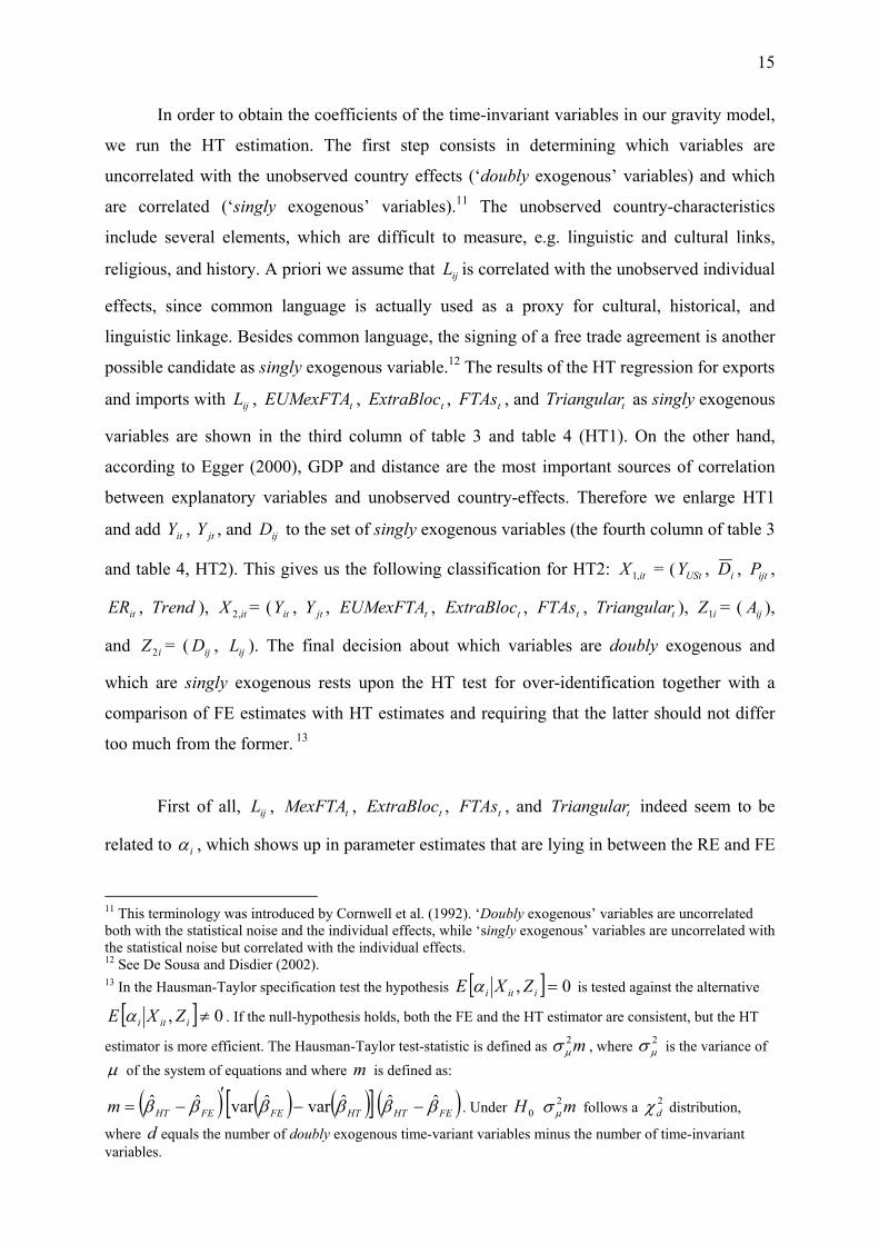
In order to obtain the coefficients of the time-invariant variables in our gravity model,
we run the HT estimation. The first step consists in determining which variables are
uncorrelated with the unobserved country effects (‘doubly exogenous’ variables) and which
are correlated (‘singly exogenous’ variables).11 The unobserved country-characteristics
include several elements, which are difficult to measure, e.g. linguistic and cultural links,
religious, and history. A priori we assume that is correlated with the unobserved individual
effects, since common language is actually used as a proxy for cultural, historical, and
linguistic linkage. Besides common language, the signing of a free trade agreement is another
possible candidate as singly exogenous variable.
ijL
t
12 The results of the HT regression for exports
and imports with , , , , and as singly exogenous
variables are shown in the third column of table 3 and table 4 (HT1). On the other hand,
according to Egger (2000), GDP and distance are the most important sources of correlation
between explanatory variables and unobserved country-effects. Therefore we enlarge HT1
and add Y , Y , and to the set of singly exogenous variables (the fourth column of table 3
and table 4, HT2). This gives us the following classification for HT2: = (Y ,
ijL tEUMexFTA
ijD
ExtraBloc tFTAs tTriangular
X
it jt
it,1 USt iD
i
, ,
, ), = (Y , , , , , ), = ( ),
and = ( , ). The final decision about which variables are doubly exogenous and
which are singly exogenous rests upon the HT test for over-identification together with a
comparison of FE estimates with HT estimates and requiring that the latter should not differ
too much from the former.
ijtP
ijAitER Trend it,2
ijL
X it jtY tEUMexFTA tExtraBloc tFTAs t ZTriangular 1
iZ2 ijD
13
First of all, , , , , and Triangular indeed seem to be
related to
ijL tMexFTA tExtraBloc tFTAs t
iα , which shows up in parameter estimates that are lying in between the RE and FE
11 This terminology was introduced by Cornwell et al. (1992). ‘Doubly exogenous’ variables are uncorrelated both with the statistical noise and the individual effects, while ‘singly exogenous’ variables are uncorrelated with the statistical noise but correlated with the individual effects. 12 See De Sousa and Disdier (2002). 13 In the Hausman-Taylor specification test the hypothesis [ ] 0, =iiti ZXE α is tested against the alternative
[ ] 0, ≠iiti ZXE α . If the null-hypothesis holds, both the FE and the HT estimator are consistent, but the HT
estimator is more efficient. The Hausman-Taylor test-statistic is defined as , where is the variance of m2µσ
2µσ
µ of the system of equations and where is defined as: m
(( ) ( ) )[ ] ( )FEHTFE ββββ ˆˆˆvarˆvar −− HTFEHTm ββ ˆˆ ′−=
d. Under follows a distribution,
where equals the number of doubly exogenous time-variant variables minus the number of time-invariant variables.
0H m2µσ
2dχ
16
estimates. Comparing HT1 and HT2 we can see that the estimation results of the latter are far
closer to the FE estimation results, both for imports and exports. In most cases, the estimated
parameter values of HT2 are identical to the FE results at the second digit numbers after the
comma. Moreover, in contrast to HT1, the HT test for over-identification does not reject the
hypothesis of legitimacy of our set of instruments. The results indicate that not only language
and the signing of a FTA are important sources of correlation between explanatory variables
and unobserved country-effects, but also GDP and distance.
Furthermore, the HT approach allows us to estimate the impact of time-invariant
effects on bilateral exports and imports, and in addition the coefficients are more efficient
than the FE approach. According to the RE approach the coefficients of common border and
common language have the expected positive sign and are statistically significant. Yet, the
Hausman test revealed that these estimates are biased. Elimination of the correlation between
some explanatory variables and the individual effects has as effect that both the common
border and common language dummies lose their statistical significance.
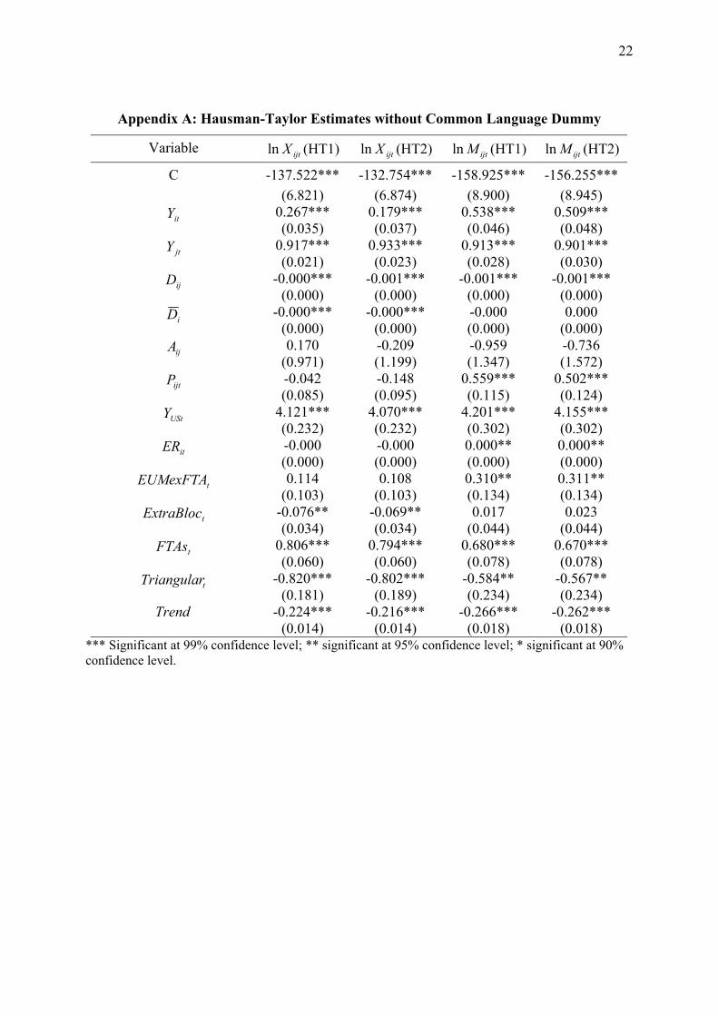
Finally, as expected a priori, the estimation results show that distance has a negative
effect on exports and imports, however negligible in economic terms. Remarkably is that once
, , and are included in the set of singly exogenous variables, the impact of distance
becomes insignificant. As Serlenga and Shin (2004) argue this result might be due to
correlation between distance and common border, since these dummies both proxy
geographical distance. However, in our gravity model the correlation between these dummies
is not the problem (the correlation coefficient between distance and common border is about
0,19). On the other hand, Egger (2000) and De Sousa and Disdier (2002) find a coefficient for
distance that is high in absolute value and statistically significant when applying the
Hausman-Taylor estimator. However, these two studies have in common that they omit the
language variable in their gravity model. As Frankel et al. (1995) show, common language is
an important determinant of bilateral trade, and omitting this variable would lead to biased
estimates of the gravity model. As a test we run the HT estimation again for both instrument
sets HT1 and HT2, but this time without the common language variable (the results can be
found in Appendix A). The results confirm our assumption; distance becomes significant in
the case of HT1 as well as HT2, both for imports and exports.
itY jtY ijD

17
Taking into account the specific characteristics of the Mexican trade, the insignificant
results for the variable distance and the dummies language and border, are actually not
surprising in this application. As said in the first section, the United States is Mexico’s biggest
trading partner, with 70 to 80 percent of Mexican total trade. As a consequence, the results of
the regressions are highly influenced by the effects of trade between the US and Mexico. First
of all, the US has a different language than Mexico, but is still Mexico’s main trading partner,
which leads to an insignificant coefficient of the language dummy. Secondly, the variable
distance used in this application is calculated following the great circle formula, which uses
latitudes and longitudes of the most important cities/agglomerations (in terms of population).
In the case of Mexico and the US is the actual distance for trade much smaller, since most of
the trade takes places at the border, dominated by the Maquiladoras. As a consequence, the
coefficient of the distance variable also turns out to be insignificant.
4 CONCLUSION
In this empirical study we used a gravity model for import and export flows to
quantify the trade effects of the EU-Mexico FTA. Besides the fixed effects approach we
applied the instrumental variables estimator developed by Hausman and Taylor (1981). An
important benefit of this approach is that it allows us to estimate time-invariant variables.
Moreover this method uses instruments derived from the structural equation, and thus avoids
using external instrumental variables. This permits controlling in an efficient way for the
individual effects and offers a better estimation of the gravity model than the conventional
approaches based on random effects or fixed effects.
Since our results clearly illustrated that the coefficients for imports and exports differ
substantially, we analyzed the gravity equation separately for imports and exports. In
particular, the results indicate that the EU-Mexico FTA had a positive trade creation effect on
imports between Mexico and the 15 members of the EU. Moreover, there is no evidence for
trade diversion, or put in other words, the trade creation effect did not come at the expense of
lower extra-bloc imports. On the other hand, in the case of exports the results are not
significant. Furthermore, our application confirms the common finding from the regional
integration literature that regional trade agreements have positive trade effects. In addition,
other triangular FTAs - a country with which both the US and the EU have signed a FTA -
tend to have a negative impact on both imports and exports of the EU and Mexico. Finally,
the time-invariant variables that we were able to estimate using the Hausman-Taylor estimator

18
turned out to be insignificant for imports as well as for exports. In general, US GDP appears
to be the most important factor in determining EU and Mexican trade flows.
Table 3: Gravity Estimation Results with Log of Bilateral Imports as Dependent
Variable (1980-2003)
Variable RE FE HT1 HT2
C -184.149*** (8.787)
-140.965*** (9.632)
-162.274*** (8.866)
-131.626*** (12.302)
itY 0.741*** (0.039)
0.431*** (0.050)
0.549*** (0.047)
0.432*** (0.049)
jtY 1.078*** (0.019)
0.858*** (0.031)
0.923*** (0.028)
0.859*** (0.031)
ijD -0.000*** (0.000) dropped -0.000***
(0.000) -0.002 (0.002)
iD -0.001*** (0.000)
-0.000*** (0.000)
-0.000* (0.000)
0.000*** (0.000)
ijL 1.826*** (0.191) dropped -3.417
(4.645) 90.362
(83.017) ijA 1.378***
(0.403) dropped 2.760 (1.738)
-31.764 (30.812)
ijtP 0.601*** (0.053)
-0.212 (0.210)
0.498*** (0.118)
-0.191 (0.203)
UStY 4.833*** (0.305)
3.908*** (0.309)
4.254*** (0.301)
3.911*** (0.302)
itER 0.000 (0.000)
-0.000** (0.000)
0.000** (0.000)
0.000** (0.000)
tEUMexFTA 0.179 (0.136)
0.321** (0.137)
0.290** (0.134)
0.322** (0.134)
tExtraBloc -0.102** (0.043)
0.078* (0.046)
0.002 (0.044)
0.078* (0.045)
tFTAs 0.815*** (0.073)
0.642*** (0.080)
0.679*** (0.078)
0.643*** (0.078)
tTriangular -0.759*** (0.236)
-0.480** (0.239)
-0.583*** (0.234)
-0.483** (0.234)
Trend -0.313 (0.019)
-0.238 (0.019)
-0.269*** (0.018)
-0.239*** (0.019)
Observations 54663 54663 54663 54663 Wald ( )142χ 3564.21 3066.05
Hausman-Taylor Over-identification Test:a)
132.27*** 0.21
*** Significant at 99% confidence level; ** significant at 95% confidence level; * significant at 90% confidence level. a) 2
dχ with d = 4 for HT1 and d = 2 for HT2.

19
Table 4: Gravity Estimation Results with Log of Bilateral Exports as Dependent
Variable (1980-2003)
Variable RE FE HT1 HT2
C -157.476*** (6.764)
-110.426*** (7.396)
-144.84*** (6.755)
-101.501*** (11.992)
itY 0.608*** (0.029)
0.103*** (0.038)
0.327*** (0.035)
0.103*** (0.038)
jtY 0.964*** (0.015)
0.874*** (0.024)
0.944*** (0.021)
0.875*** (0.024)
ijD -0.000*** (0.000) dropped -0.000***
(0.000) -0.002 (0.002)
iD -0.001*** (0.000)
-0.000 (0.000)
-0.001*** (0.000)
0.000 (0.000)
ijL 2.105*** (0.149) dropped 6.735***
(2.520) 98.647
(103.207) ijA 1.168***
(0.313) dropped -0.202 (0.950)
-33.733 (38.412)
ijtP 0.126*** (0.041)
-1.240*** (0.161)
0.014 (0.073)
-1.225*** (0.157)
UStY 4.466*** (0.235)
3.861*** (0.237)
4.259*** (0.232)
3.861*** (0.232)
itER -0.000 (0.000)
-0.000*** (0.000)
-0.000 (0.000)
-0.000 (0.000)
tEUMexFTA 0.055 (0.105)
0.082 (0.106)
0.085 (0.104)
0.083 (0.104)
tExtraBloc -0.126*** (0.033)
-0.031 (0.035)
-0.108*** (0.034)
-0.031 (0.034)
tFTAs 0.788*** (0.057)
0.750*** (0.062)
0.817*** (0.061)
0.751*** (0.060)
tTriangular -0.804*** (0.183)
-0.674*** (0.185)
-0.845*** (0.181)
-0.676*** (0.181)
Trend -0.262*** (0.014)
-0.190*** (0.015)
-0.234*** (0.014)
-0.190*** (0.014)
Observations 54944 54944 54944 54944 Wald ( )142χ 7548.58 6235.60
Hausman-Taylor Over-identification Test:a)
318.04*** 0.17
*** Significant at 99% confidence level; ** significant at 95% confidence level; * significant at 90% confidence level. a) 2
dχ with d = 4 for HT1 and d = 2 for HT2.
20
5 BIBLIOGRAPHY Bayoumi, T. and Eichengreen, B. (1995), “Is Regionalism Simply a Diversion? Evidence from
the Evolution of the EC and EFTA”, NBER Working Paper 5283, Cambridge, MA.
Cornwell, C., Schmidt, P. and Wyhowski, D. (1992), “Simultaneous Equations and Panel
Data”, Journal of Econometrics 51(1-2), pp. 151-181.
De Sousa, J. and Disdier, A. (2002), "Trade, Border Effects, and Individual Characteristics: a
Proper Specification”, Unpublished Manuscript, University of Paris 1.
Deardorff, A. (1984), “Testing Trade Theories and Predicting Trade Flows”, in Jones, R. and
Kenen, P. (eds.), Handbook of International Economics 1, Elsevier Science Publishers,
Amsterdam.
Dhar, S. and Panagariya, A. (1999), “Is East Asia Less Open Than North America and the
EEC? No.” In Piggott, J. and Woodland, A. (eds.), International Trade Policy and the
Pacific Rim, London, Macmillan.
Egger, P. (2000), “On the Problem of Endogenous Unobserved Effects in the Estimation of
Gravity Models”, WIFO-Working Paper 132/2000.
Egger, P. (2002), “An Econometric View on the Estimation of Gravity Models and the
Calculation of Trade Potentials”, The World Economy, 25, pp.297-312.
EU (2000), “Decision No 2/2000 of the EU-Mexico Joint Council”, Official Journal of the
European Communities, 2000/415/EC. Available at: http://europe.eu.int.
Frankel, J. (1997), “Regional Trading Blocs in the World Economic System”, Institute for
International Economics, Washington, D.C.
Frankel, J., Stein, E. and Wei, S. (1995), “Trading Blocs and the Americas: The Natural, the
Unnatural and the Super-Natural”, Journal of Development Economics (47), pp.61-
95.
Gambrill, M. (2002), “International Subcontracting Trade in the EU-Mexico Free Trade
Agreement”, in Georgakopoulos, T., Paraskevopoulos, C., and Smithin, J., (eds.),
Globalization and Economic Growth: A Critical Evaluation, APF Press, Toronto,
Canada.
Harrigan, J. (2002), “Specialisation and the Volume of Trade: Do the Data Obey the Laws?”
In Choi, K. and Harrigan, J. (eds.), The Handbook of International Trade, Blackwell.
Hausman, J. (1978), “Specification Tests in Econometrics”, Econometrica 46(6), pp.1251-
1271.
Hausman, J. and Taylor, W. (1981), “Panel Data and Unobserved Individual Effects”,
Econometrica 49(6), pp.1377-1398.

21
Helpman, E. (1987), “Imperfect Competition and International Trade: Evidence From
Fourteen Industrial Countries”, Journal of Japanese and International Economics 1,
pp.62-81.
Helpman, E. and Krugman, P. (1985), “Market Structure and Foreign Trade: Increasing
Returns, Imperfect Competition and the International Economy”, Cambridge, MIT
Press.
Linneman, H. (1966), “An Econometric Study of International Trade Flows”, North Holland,
Amsterdam.
Mátyás, L. (1997), “Proper Econometric Specification of the Gravity Model”, The World
Economy 20(3), pp.363-368.
Serlenga, L. and Shin, Y. (2004), “Gravity Models of the Intra-EU Trade: Application of the
Hausman-Taylor Estimation in Panels with Heterogenous Time-Specific Common
Factors”, Unpublished Manuscript, University of Edingburgh.
WTO (2000), “Mapping of Regional Trade Agreements”, World Trade Organization
WT/REG/W/41, October 2000.
22
Appendix A: Hausman-Taylor Estimates without Common Language Dummy
Variable ijtXln (HT1) ijtXln (HT2) ijtMln (HT1) ijtMln (HT2)
C -137.522*** (6.821)
-132.754*** (6.874)
-158.925*** (8.900)
-156.255*** (8.945)
itY 0.267*** (0.035)
0.179*** (0.037)
0.538*** (0.046)
0.509*** (0.048)
jtY 0.917*** (0.021)
0.933*** (0.023)
0.913*** (0.028)
0.901*** (0.030)
ijD -0.000*** (0.000)
-0.001*** (0.000)
-0.001*** (0.000)
-0.001*** (0.000)
iD -0.000*** (0.000)
-0.000*** (0.000)
-0.000 (0.000)
0.000 (0.000)
ijA 0.170 (0.971)
-0.209 (1.199)
-0.959 (1.347)
-0.736 (1.572)
ijtP -0.042 (0.085)
-0.148 (0.095)
0.559*** (0.115)
0.502*** (0.124)
UStY 4.121*** (0.232)
4.070*** (0.232)
4.201*** (0.302)
4.155*** (0.302)
itER -0.000 (0.000)
-0.000 (0.000)
0.000** (0.000)
0.000** (0.000)
tEUMexFTA 0.114 (0.103)
0.108 (0.103)
0.310** (0.134)
0.311** (0.134)
tExtraBloc -0.076** (0.034)
-0.069** (0.034)
0.017 (0.044)
0.023 (0.044)
tFTAs 0.806*** (0.060)
0.794*** (0.060)
0.680*** (0.078)
0.670*** (0.078)
tTriangular -0.820*** (0.181)
-0.802*** (0.189)
-0.584** (0.234)
-0.567** (0.234)
Trend -0.224*** (0.014)
-0.216*** (0.014)
-0.266*** (0.018)
-0.262*** (0.018)
*** Significant at 99% confidence level; ** significant at 95% confidence level; * significant at 90% confidence level.
Related Documents


