UNIVERSITY OF CALGARY Tracking Thermal and Structural Properties of Melt-Freeze Crusts in the Seasonal Snowpack by Michael Andrew Smith A DISSERTATION SUBMITTED TO THE FACULTY OF GRADUATE STUDIES IN PARTIAL FULFILLMENT OF THE REQUIREMENTS FOR THE DEGREE OF DOCTOR OF PHILOSOPHY DEPARTMENT OF CIVIL ENGINEERING CALGARY, ALBERTA May, 2014 c Michael Andrew Smith 2014

Welcome message from author
This document is posted to help you gain knowledge. Please leave a comment to let me know what you think about it! Share it to your friends and learn new things together.
Transcript

UNIVERSITY OF CALGARY
Tracking Thermal and Structural Properties of Melt-Freeze Crusts in the Seasonal
Snowpack
by
Michael Andrew Smith
A DISSERTATION
SUBMITTED TO THE FACULTY OF GRADUATE STUDIES
IN PARTIAL FULFILLMENT OF THE REQUIREMENTS FOR THE
DEGREE OF DOCTOR OF PHILOSOPHY
DEPARTMENT OF CIVIL ENGINEERING
CALGARY, ALBERTA
May, 2014
c© Michael Andrew Smith 2014

Abstract
Persistent weak layers present a particular challenge for avalanche forecasters due to their
long lifetime and the difficulty of obtaining observations once they are deeply buried. Melt-
freeze crusts are one type of persistent weak layer that is often associated with deep slab
avalanches during late winter or spring. This study seeks to improve the understanding of
the thermal and structural properties of melt-freeze crusts by tracking them from formation
through to isothermal conditions in the spring.
Specific Surface Area (SSA) was tracked weekly using near-infrared digital photography
for nine natural crusts and four cold lab crusts during the winters of 2008-09 and 2009-10.
Image analysis techniques were adapted from existing methods in order to track the mean
SSA for specific structures within crusts, as well as vertical profiles of SSA across crust
boundaries. Few temporal trends were identified even in the presence of strong diurnal slope
normal temperature gradients, but the ratio of mean SSA between crusts and adjacent layers
did reveal relative changes in the structure.
The thermal conductivity was tracked for six natural and five cold lab crusts during
the winter of 2009-10 using a heated needle probe. Thermal conductivity of two cold lab
crusts increased during freezing and subsequently decreased in the presence of strong vertical
temperature gradients, while that of natural crusts had no discernible trends under weak
temperature gradients. Trends of increasing thermal conductivity in adjacent layers were
well correlated with increasing density as in previous studies but with a positive offset that
may be attributable to the warmer snow temperatures in this study relative to past studies.
The SNOWPACK model was used to model the formation and evolution of spatially
uniform crusts at a flat study plot as well as on a virtual slope. Persistent model cold
temperature biases were found on the virtual slope, which resulted in delays in settling and
densification relative to observations. A warm model bias was found for the flat simulation,
ii

and settling and layer water content exceeded what was observed. Both biases were likely
related to meteorological inputs.
iii

Acknowledgements
First and foremost I would like to thank my supervisor Bruce Jamieson, whose timely advice
and seemingly endless patience have allowed me to complete this dissertation.
My fellow graduate students at ASARC kept the mood light after long days in the field
and put in long, cold hours in the pit while gathering the data for study: Thomas Exner,
Katherine Johnston, Cam Ross, Cora Shea and Dave Tracz. The dry humour and sage
advice of Post-Doc Sascha Bellaire helped me steer through the final season of field work,
while ASARC technicians Catherine Brown, Ali Haeri and Mark Kolasinski were always
helpful in gathering data and refining field methods.
The staff of the Avalanche Control Section at Glacier National Park, specifically forecast-
ers Bruce McMahon and Jeff Goodrich, provided invaluable logistical support and guidance
during my three winters of work. Without their assistance this study could not have been
completed. Mike Wiegele and his staff at Mike Wiegele heli-skiing have been long-time
supporters of snow science and of ASARC in particular. The snow safety staff at Kicking
Horse Mountain Resort were unfailingly accommodating in providing an alternate venue
when conditions did not cooperate at Rogers Pass.
I would like to thank Charles Fierz for his help in getting SNOWPACK up and running,
and for helping me to understand the guts of the model. John Kelly and Ilya Storm of
the Canadian Avalanche Centre were also instrumental in pushing me toward using the
SNOWPACK model as part of my research.
For help with seemingly endless edits and revisions I must once again thank Bruce
Jamieson as well as ASARC Post-Doc Michael Schirmer for his valuable insight late in
the writing process.
I must also thank the long list of avalanche professionals and researchers who provided
ideas, insight and inspiration. You’re too numerous to list, but I hope to repay the favor as
iv

I move forward. Finally I’d like to thank my family and friends who never gave up on me
even when completion seemed years away.
v

Table of Contents
Abstract . . . . . . . . . . . . . . . . . . . . . . . . . . . . . . . . . . . . . . . . . ii
Acknowledgements . . . . . . . . . . . . . . . . . . . . . . . . . . . . . . . . . . . iv
Table of Contents . . . . . . . . . . . . . . . . . . . . . . . . . . . . . . . . . . . . vi
List of Tables . . . . . . . . . . . . . . . . . . . . . . . . . . . . . . . . . . . . . . ix
List of Figures . . . . . . . . . . . . . . . . . . . . . . . . . . . . . . . . . . . . . . x
1 Introduction . . . . . . . . . . . . . . . . . . . . . . . . . . . . . . . . . . . . 1
1.1 The Seasonal Snowpack . . . . . . . . . . . . . . . . . . . . . . . . . . . . . 3
1.2 Research Goals . . . . . . . . . . . . . . . . . . . . . . . . . . . . . . . . . . 8
1.3 Research Methods . . . . . . . . . . . . . . . . . . . . . . . . . . . . . . . . . 10
2 Thermal Conductivity . . . . . . . . . . . . . . . . . . . . . . . . . . . . . . 16
2.1 Non-steady-state thermal conductivity theory . . . . . . . . . . . . . . . . . 17
2.2 Past Measurements . . . . . . . . . . . . . . . . . . . . . . . . . . . . . . . . 20
2.3 Modeling . . . . . . . . . . . . . . . . . . . . . . . . . . . . . . . . . . . . . . 22
2.4 Equipment . . . . . . . . . . . . . . . . . . . . . . . . . . . . . . . . . . . . . 26
2.5 Field Methods . . . . . . . . . . . . . . . . . . . . . . . . . . . . . . . . . . . 28
2.6 Results and Analysis . . . . . . . . . . . . . . . . . . . . . . . . . . . . . . . 30
2.6.1 Thermal conductivity by grain type . . . . . . . . . . . . . . . . . . . 33
2.6.2 Thermal conductivity and physical parameters . . . . . . . . . . . . . 39
2.6.3 Thermal conductivity by site . . . . . . . . . . . . . . . . . . . . . . . 47
2.6.4 Spatial variability of thermal conductivity . . . . . . . . . . . . . . . 61
2.7 Chapter Summary . . . . . . . . . . . . . . . . . . . . . . . . . . . . . . . . 64
3 Near Infrared Photography . . . . . . . . . . . . . . . . . . . . . . . . . . . . 67
3.1 Specific surface area (SSA) theory and past studies using optical methods . . 67
3.2 Equipment and Field Methods . . . . . . . . . . . . . . . . . . . . . . . . . . 70
vi

3.3 Analysis Methods . . . . . . . . . . . . . . . . . . . . . . . . . . . . . . . . . 74
3.4 Results and Discussion . . . . . . . . . . . . . . . . . . . . . . . . . . . . . . 78
3.4.1 2008-09 Crusts . . . . . . . . . . . . . . . . . . . . . . . . . . . . . . 79
3.4.2 2009-10 Crusts: Field . . . . . . . . . . . . . . . . . . . . . . . . . . . 85
3.4.3 2009-10 Crusts: Cold Lab . . . . . . . . . . . . . . . . . . . . . . . . 94
3.4.4 Spatial variation of specific surface area (SSA) on a planar slope . . . 103
3.5 Chapter Summary . . . . . . . . . . . . . . . . . . . . . . . . . . . . . . . . 108
3.6 Recommendations for future studies . . . . . . . . . . . . . . . . . . . . . . . 110
4 Snowpack Modeling . . . . . . . . . . . . . . . . . . . . . . . . . . . . . . . . 112
4.1 Literature Review . . . . . . . . . . . . . . . . . . . . . . . . . . . . . . . . . 112
4.2 The SNOWPACK model . . . . . . . . . . . . . . . . . . . . . . . . . . . . . 115
4.3 SNOWPACK Simulations . . . . . . . . . . . . . . . . . . . . . . . . . . . . 119
4.3.1 SNOWPACK configuration . . . . . . . . . . . . . . . . . . . . . . . 120
4.3.2 South Run 2009 Crusts . . . . . . . . . . . . . . . . . . . . . . . . . . 121
4.3.3 South Run 2009 Crusts Discussion . . . . . . . . . . . . . . . . . . . 134
4.3.4 FI100308 . . . . . . . . . . . . . . . . . . . . . . . . . . . . . . . . . . 135
4.3.5 FI100308 Discussion . . . . . . . . . . . . . . . . . . . . . . . . . . . 140
4.4 Chapter Summary . . . . . . . . . . . . . . . . . . . . . . . . . . . . . . . . 142
4.5 Recommendations for future studies . . . . . . . . . . . . . . . . . . . . . . . 145
5 Conclusions . . . . . . . . . . . . . . . . . . . . . . . . . . . . . . . . . . . . 147
5.1 Temporal trends of SSA and thermal conductivity . . . . . . . . . . . . . . . 147
5.2 Modeling observations with SNOWPACK . . . . . . . . . . . . . . . . . . . . 149
5.3 Spatial variability of SSA and thermal conductivity . . . . . . . . . . . . . . 150
5.4 Thermal conductivity, grain type, density and temperature . . . . . . . . . . 151
5.5 Use of SSA to quantify the structure of melt-freeze crusts . . . . . . . . . . . 151
5.6 Use of a thermal conductivity probe in melt-freeze crusts . . . . . . . . . . . 152
vii

5.7 Contributions to snow science . . . . . . . . . . . . . . . . . . . . . . . . . . 152
6 Recommendations for Future Research . . . . . . . . . . . . . . . . . . . . . 154
6.1 Thermal Conductivity . . . . . . . . . . . . . . . . . . . . . . . . . . . . . . 154
6.2 Specific Surface Area . . . . . . . . . . . . . . . . . . . . . . . . . . . . . . . 155
6.3 Modeling . . . . . . . . . . . . . . . . . . . . . . . . . . . . . . . . . . . . . . 156
Bibliography . . . . . . . . . . . . . . . . . . . . . . . . . . . . . . . . . . . . . . 157
A Description of study sites and narratives of crust formation and evolution . . 170
A.1 2007-08 Crust . . . . . . . . . . . . . . . . . . . . . . . . . . . . . . . . . . . 174
A.2 2008-09 Crusts . . . . . . . . . . . . . . . . . . . . . . . . . . . . . . . . . . 176
A.3 2009-10 Crusts . . . . . . . . . . . . . . . . . . . . . . . . . . . . . . . . . . 179
B Glossary . . . . . . . . . . . . . . . . . . . . . . . . . . . . . . . . . . . . . . 184
C Thermal Conductivity and Layer Characteristics . . . . . . . . . . . . . . . . 189
viii

List of Tables
1.1 Properties recorded in a snow profile . . . . . . . . . . . . . . . . . . . . . . 5
2.1 A summary of published values of snow thermal conductivity since 1997 . . . 22
2.2 Observation period and number of thermal conductivity measurements . . . 31
2.3 Thermal conductivity and density by grain type . . . . . . . . . . . . . . . . 34
2.4 Thermal conductivity by grain type with and without outliers . . . . . . . . 36
2.5 Thermal conductivity for crust samples, by site . . . . . . . . . . . . . . . . 37
2.6 Significant correlations between thermal conductivity and density . . . . . . 40
2.7 Significant correlations between thermal conductivity and layer temperature 43
2.8 Correlations between thermal conductivity and temperature, dry and moist . 44
2.9 Pearson correlations between λ, density and layer temperature . . . . . . . . 49
2.10 Pearson correlations between λ, ρ and T above and below FI0308 . . . . . . 51
2.11 Pearson correlations: rate of change of λ, layer T and TG for LAB0413 . . . 57
3.1 Correlations of SSA, NIR with other crust properties . . . . . . . . . . . . . 84
4.1 Parameters used to initialize SNOWPACK . . . . . . . . . . . . . . . . . . . 117
4.2 SNOWPACK iterations for SR20090305 . . . . . . . . . . . . . . . . . . . . 122
4.3 SNOWPACK iterations for FI20091208 . . . . . . . . . . . . . . . . . . . . . 136
A.1 Study Sites in Rogers Pass . . . . . . . . . . . . . . . . . . . . . . . . . . . . 172
B.1 Grain type abbreviations . . . . . . . . . . . . . . . . . . . . . . . . . . . . . 186
C.1 Layer characteristics for 2008-09 crusts . . . . . . . . . . . . . . . . . . . . . 189
C.2 Thermal conductivity and layer characteristics for 2009-10 crusts . . . . . . . 190
C.3 All thermal conductivity measurements . . . . . . . . . . . . . . . . . . . . . 208
ix

List of Figures and Illustrations
1.1 Snow profile example . . . . . . . . . . . . . . . . . . . . . . . . . . . . . . . 4
1.2 Example of vapour transfer under low temperature gradients . . . . . . . . . 7
1.3 Example of thermistor and thermocouple placement . . . . . . . . . . . . . . 11
2.1 Schematic of the Hukseflux TP02 . . . . . . . . . . . . . . . . . . . . . . . . 27
2.2 Annotated NIR photograph of TP02 sampling locations . . . . . . . . . . . . 29
2.3 A typical plot of ln(t) versus the nominal rise in temperature . . . . . . . . . 33
2.4 Box Whisker plot of thermal conductivity by grain type . . . . . . . . . . . . 35
2.5 Thermal conductivity versus density . . . . . . . . . . . . . . . . . . . . . . 40
2.6 λ versus density for faceted (FC) grain types with outliers removed . . . . . 41
2.7 λ versus density for rounded (RG) grains . . . . . . . . . . . . . . . . . . . . 42
2.8 λ versus temperature . . . . . . . . . . . . . . . . . . . . . . . . . . . . . . . 43
2.9 λ versus temperature for melt-freeze forms . . . . . . . . . . . . . . . . . . . 44
2.10 Quadratic model fit for all dry non-melt-freeze samples of λ . . . . . . . . . 45
2.11 λ in the layer above the FI0109 crust . . . . . . . . . . . . . . . . . . . . . . 49
2.12 λ in the layer below the FI0109 crust . . . . . . . . . . . . . . . . . . . . . . 50
2.13 λ in the layer above the FI0308 crust . . . . . . . . . . . . . . . . . . . . . . 51
2.14 λ in the layer below the FI0308 crust . . . . . . . . . . . . . . . . . . . . . . 52
2.15 λ in the layer above the RP0112 crust . . . . . . . . . . . . . . . . . . . . . 53
2.16 λ in the layer below the RP0112 crust . . . . . . . . . . . . . . . . . . . . . 54
2.17 Schematic of the insulated box used for cold lab experiments. . . . . . . . . . 55
2.18 Time series of λ measurements for LAB0410 . . . . . . . . . . . . . . . . . . 56
2.19 Time series of λ measurements for LAB0413 . . . . . . . . . . . . . . . . . . 57
2.20 Average T and TG for LAB0413 . . . . . . . . . . . . . . . . . . . . . . . . . 58
2.21 Montage of thermal IR images of crust LAB0413 . . . . . . . . . . . . . . . . 59
x

2.22 Thermal IR image at 99 hours . . . . . . . . . . . . . . . . . . . . . . . . . . 60
2.23 Site used to evaluate spatial variability . . . . . . . . . . . . . . . . . . . . . 62
2.24 λ measurements on a south-facing slope . . . . . . . . . . . . . . . . . . . . . 63
3.1 Typical field setup for near-infrared photography . . . . . . . . . . . . . . . 72
3.2 Flow chart for flat field correction . . . . . . . . . . . . . . . . . . . . . . . . 75
3.3 Increase in coefficient of variation (CV) due to image processing . . . . . . . 77
3.4 Rejected NIR image . . . . . . . . . . . . . . . . . . . . . . . . . . . . . . . 77
3.5 SSA time series for crust SR090127 . . . . . . . . . . . . . . . . . . . . . . . 80
3.6 SSA time series for crust SR090222 . . . . . . . . . . . . . . . . . . . . . . . 81
3.7 SSA time series for crust SR090301 . . . . . . . . . . . . . . . . . . . . . . . 83
3.8 SSA image of CR100109 . . . . . . . . . . . . . . . . . . . . . . . . . . . . . 86
3.9 SSA time series for crust RP100112 . . . . . . . . . . . . . . . . . . . . . . . 87
3.10 SSA time series for crust BV100112 . . . . . . . . . . . . . . . . . . . . . . . 88
3.11 SSA time series for crust FI100308 . . . . . . . . . . . . . . . . . . . . . . . 90
3.12 A month of mean vertical SSA for FI100308 . . . . . . . . . . . . . . . . . . 91
3.13 Ratio of areal averaged SSA for FI100308 . . . . . . . . . . . . . . . . . . . . 92
3.14 Schematic of insulated cold lab box . . . . . . . . . . . . . . . . . . . . . . . 95
3.15 SSA time series for crust LAB100330 . . . . . . . . . . . . . . . . . . . . . . 96
3.16 SSA time series for crust LAB100409 . . . . . . . . . . . . . . . . . . . . . . 97
3.17 SSA time series for crust LAB100410 . . . . . . . . . . . . . . . . . . . . . . 99
3.18 SSA time series for crust LAB100413 . . . . . . . . . . . . . . . . . . . . . . 100
3.19 Spatial variability of SSA at 2008-09 South Run site . . . . . . . . . . . . . . 104
3.20 Spatial variability of vertical profiles of SSA at 2008-09 South Run site . . . 105
3.21 Spatial variability of vertical profiles of CV at 2008-09 South Run site . . . . 107
4.1 SNOWPACK Grain Matrix . . . . . . . . . . . . . . . . . . . . . . . . . . . 116
4.2 Evolution of snow depth and grain type for simulation SR20090305-1 . . . . 123
xi

4.3 Measured versus modeled layer depth for SR090301, SR090222 and SR090301 124
4.4 Measured versus simulated density and layer temperature for SR090127 . . . 125
4.5 Measured versus simulated specific surface area for SR090127 . . . . . . . . . 126
4.6 Measured versus simulated density and layer temperature for SR090222 . . . 128
4.7 Measured versus simulated specific surface area for SR090222 . . . . . . . . . 129
4.8 Measured versus simulated density and layer temperature for SR090301 . . . 130
4.9 Measured versus simulated specific surface area for SR090301 . . . . . . . . . 131
4.10 Measured versus simulated specific surface area from run SR20090305-2 . . . 132
4.11 Hardness index from simulation SR20090305-1 . . . . . . . . . . . . . . . . . 133
4.12 Evolution in snow depth and grain type for simulation FI20091208-2 . . . . . 137
4.13 Measured versus simulated HS, depth and temperature for crust FI100308 . 139
4.14 Measured versus simulated specific surface area for FI100308 . . . . . . . . . 140
4.15 Measured versus simulated thermal conductivity for FI100308 . . . . . . . . 141
A.1 Mountains of western British Columbia . . . . . . . . . . . . . . . . . . . . . 171
A.2 Topography and location around study areas referenced in this dissertation . 171
A.3 Topography and location of landmarks surrounding Rogers Pass . . . . . . . 173
A.4 Area surrounding Mt. Fidelity study plot . . . . . . . . . . . . . . . . . . . . 173
A.5 Hourly air temperature and precipitation, CR071205 . . . . . . . . . . . . . 175
A.6 Air temperature and daily precipitation winter 2007-08 . . . . . . . . . . . . 176
A.7 Air temperature and daily precipitation winter 2008-09 . . . . . . . . . . . . 177
A.8 Incoming shortwave and net longwave radiation, winter 2008-09 . . . . . . . 178
A.9 Air temperature and daily precipitation, winter 2009-10 . . . . . . . . . . . . 180
A.10 Incoming shortwave and net longwave radiation, winter 2009-10 . . . . . . . 180
A.11 Air temperature and daily precipitation, Rogers Pass winter 2009-10 . . . . . 181
xii

Chapter 1
Introduction
Snow is an intriguing material to study: Unlike many materials, it exists within several
degrees (or at most several tens of degrees) of its melting point; Unlike metamorphic rock,
snow may undergo significant metamorphism over the course of several hours, often to the
chagrin of avalanche forecasters. According to data published by the Canadian Avalanche
Centre (CAA, 2014) and drawn from Jamieson et al. (2010) avalanches in Canada were
responsible for an average of 14 fatalities per year from 1996 -2007. This represents an
increase of 4 fatalities per year over the previous 10-year period (Jamieson and Geldsetzer,
1996). Several winters since then have exceeded the average with the majority of victims
comprised of winter recreationists.
Numerous regional or national public avalanche forecast centres provide public avalanche
bulletins in hopes of educating users and reducing the number of incidents. Avalanche fore-
casters typically draw on professional experience to synthesize information from avalanche
professionals and, increasingly, public observations. Class I data, the “stability factors”
(McClung and Schaerer, 2006) include the most direct signs of snowpack stability such as
recent avalanche activity and stability or explosives tests. Class II data, the “snowpack fac-
tors”, include past avalanche observations and information from snow profiles (see Section
1.1. Class III data are the “meteorological factors” such as recent precipitation, wind and
temperature.
In Canada and the United States the avalanche danger is communicated via the North
American Public Avalanche Danger Scale. There are five possible levels of danger, from
“Low” to “Extreme” and within each level the forecaster communicates travel advice, the
size and distribution of avalanches, and the likelihood of avalanches. The likelihood is further
1
divided into natural and human-triggered avalanches.
The largest and most destructive avalanches are slab avalanches, wherein a failure within
the snowpack releases an overlying cohesive slab of snow. Reduced to the most simple fac-
tors, stress applied to a given layer exceeds its strength. From the standpoint of forecasting,
the likelihood of an avalanche may be reduced to two factors: The probability of a localized
failure in a particular layer, and the probability that the failure will propagate (the propa-
gation propensity, Gauthier and Jamieson (2008)) far enough for the overlying slab to fail.
Triggering may occur through heavy snowfall, dynamic loading by a skier or snowmobiler,
explosives or warming, leading to increased strain rates within weak layers. Propagation
propensity is a property of both the failure layer and the overlying slab, where energy is
released through shear failure and weak layer collapse (Heierli and Zaiser, 2008) and if the
energy released exceeds the fracture toughness of the failure layer, the failure will continue
to propagate.
One particular challenge for all avalanche professionals is the persistent weak layer
(PWL). As its name suggests this is a weakness in the snowpack that is buried and persists
for weeks or even months. Oftentimes such layers will become deeply buried and unreactive
for long periods before suddenly becoming reactive once again. A PWL is often difficult to
observe due to its depth in the snowpack and forecasters are left with little information or
warning to when it may release slab avalanches.
Melt-freeze crusts, especially those that form early in the winter, are a frequent source
of concern (e.g. Smith et al., 2008) that may lie dormant throughout the winter before
failing as the snowpack weakens, or as it is stressed by large dynamic loads such as cornice
failures. Crusts are unique from other snow grain types in their microstructure, persistence
and ability to resist compaction. This may contribute to the formation of weak facet layers
while freezing, as a strong temperature gradient is maintained between the wetted layer and
a new snow layer above (e.g. Jamieson and Fierz, 2004) and also once buried due to their
2

relatively high thermal conductivity and lower vapour permeability (Jamieson, 2006). Thick
or stiff crusts may also act as a bed surface for avalanches, where shear stress is concentrated
(Habermann et al., 2008). Numerous studies have documented the formation and role of
melt-freeze crusts in avalanches (Buhler, 2013; Conlan and Jamieson, 2012; Jamieson and
Langevin, 2004; Jamieson, 2004a,b, 2006) and initial efforts have been made to understand
their formation and evolution through field and cold lab studies as well as modeling (e.g.
Jamieson and Fierz, 2004; Smith et al., 2008).
The goal of this study is to better understand the structure and temporal evolution of
melt-freeze crusts in the seasonal snowpack. The remainder of this chapter will provide a brief
introduction to the science of snow including the deposition, layering and metamorphism of
the seasonal snowpack. The research goals and methods will be outlined and the study area
introduced. The remaining chapters will examine in detail the various aspects of the study.
1.1 The Seasonal Snowpack
In North America the seasonal snowpack in mountainous regions is typically in place from
October through April or May. During this time the snow may go through several cycles
of accumulation, ablation, melting and re-freezing. Most precipitation particles have a den-
dritic form which is quickly broken down through the action of wind, sun, compaction and
metamorphic processes, leading to the formation of a layered snowpack consisting of well-
bonded rounded grains, angular faceted grains, stiff melt-freeze forms and feathery surface
hoar. Snowpack structure may also be highly spatially variable due to local variations in
weather, topography and vegetation.
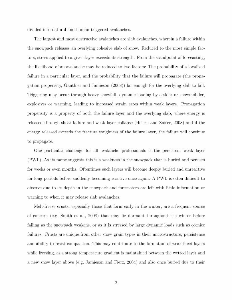
Characterization of the seasonal snowpack is usually done via snow profile (Figure 1.1
and Table 1.1) whereby a field worker exposes a pit wall of the snowpack. Layers are defined
by grain type, density, crystal form and hand hardness (CAA, 2007), and may also depend on
whether the objective is stability evaluation or research, where even small variations may be
3
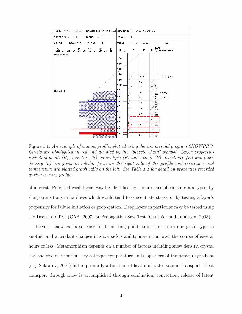
Figure 1.1: An example of a snow profile, plotted using the commercial program SNOWPRO.Crusts are highlighted in red and denoted by the “bicycle chain” symbol. Layer propertiesincluding depth (H), moisture (θ), grain type (F) and extent (E), resistance (R) and layerdensity (ρ) are given in tabular form on the right side of the profile and resistance andtemperature are plotted graphically on the left. See Table 1.1 for detail on properties recordedduring a snow profile.
of interest. Potential weak layers way be identified by the presence of certain grain types, by
sharp transitions in hardness which would tend to concentrate stress, or by testing a layer’s
propensity for failure initiation or propagation. Deep layers in particular may be tested using
the Deep Tap Test (CAA, 2007) or Propagation Saw Test (Gauthier and Jamieson, 2008).
Because snow exists so close to its melting point, transitions from one grain type to
another and attendant changes in snowpack stability may occur over the course of several
hours or less. Metamorphism depends on a number of factors including snow density, crystal
size and size distribution, crystal type, temperature and slope-normal temperature gradient
(e.g. Sokratov, 2001) but is primarily a function of heat and water vapour transport. Heat
transport through snow is accomplished through conduction, convection, release of latent
4
Table 1.1: Properties recorded in a snow profile. Geographical location, slope angle andaspect, present weather and total snow depth are also recorded.
Property Abbrev. Units NotesLayer depth H cm Measured from ground for full profiles
and from snow surface for partial (test)profiles
Temperature T ◦C Measured at surface and each 10cm thereafter and sometimes at layerboundaries
Layer density ρ kg m−3
Grain form F ∼ Symbols are detailed in Fierz et al.(2009)
Grain size (Extent) E mm Often given as a rangeLayer resistance R ∼ Varies from fist (softest) to ice (hard-
est). Also represented by horizontalbar graphs on the profile.
Liquid water con-tent
θ ∼ 5 levels, plotted on snow profiles usingvertical lines: from “dry” (no lines) to“slush” (4 lines).
Layer comments ∼ ∼ May include date when layer wasburied, which is used to track PWLs
5

heat by freezing water and radiation, though solar radiation is only significant close to
the snow surface (Bakermans and Jamieson, 2009). Greene (2007) provides a brief review
of studies regarding the importance of convection in the snowpack, most of which are in
agreement that it is important only in porous snow in the presence of a strong temperature
gradient. LaChapelle (1960) noted that the coefficient of diffusion of water vapour in snow
was four to five times that of vapour in air. This emphasized the importance of what is now
referred to as the ’hand to hand’ process of mass transport between snow crystals. In field
studies, the slope-normal temperature gradient is usually used as a proxy for heat and vapour
flux. The measured slope-normal temperature gradient is sometimes referred to as the “bulk”
temperature gradient to differentiate it from gradients that may occur on scales too small to
measure with thermistors or thermocouples. Hereafter, the terms slope-normal temperature
gradient,vertical temperature gradient and temperature gradient are used interchangeably.
Snowpack metamorphism is often classed as either Temperature Gradient or Equilibrium
metamorphism based on the bulk slope-normal temperature gradient:
Temperature Gradient (TG) Metamorphism is assumed to occur when the slope-normal
temperature gradient exceeds 10◦
C m−1. This is a frequent occurrence near the surface
of the snowpack due to relatively rapid fluctuations in the air temperature, and may occur
throughout the full depth of shallow snowpacks. In this case, vapour transport through the
snowpack arises from the bulk temperature gradient. The tendency is toward the formation
of faceted crystals with flat faces, sharp edges and poor intragranular bonding. In the
extreme case, very large edged or cupped crystals known as ’depth hoar’ may result. Layers
comprised of large facets or depth hoar are typically poorly bonded and weak and thus
represent a potential failure layer for avalanches.
Equilibrium (EQ) metamorphism is assumed when the bulk temperature gradient is less
than 10◦
C m−1. In this case, vapour transfer is driven by a vapour pressure gradient arising
from the differences in grain curvature within the snowpack, and not the bulk temperature
6

Figure 1.2: Example of vapour transfer under low temperature gradients. Adapted fromvarious figures in McClung and Schaerer (2006). The smaller grain with radius R1 will havea larger equilibrium vapour pressure Pv1 than the larger grain with radius R2. The gradientin vapour pressure will cause vapour transfer from the smaller grain to the larger grain. Thesame process will lead to grain growth at the neck between two grains.
gradient (Colbeck, 1980; Flin et al., 2003). Small grains with a smaller radius of curvature will
have a higher vapour pressure at the ice-air interface than will larger grains. This results in a
transfer of mass from small or highly dendritic grains to large grains or necks between grains,
as illustrated in Figure 1.2. This is traditionally assumed to be the dominant mechanism in
the growth of rounded, well-bonded layers. A notable exception is when grains already have
flat faces, which have a large radius of curvature: Although the edges, with a small radius
of curvature, will round, the basic form will persist at low temperature gradients (Brown
et al., 2001). These forms will be slower to round and form bonds with adjacent crystals, and
indeed layers of faceted crystals tend to persist long after the strong temperature gradient
disappears (Jamieson and Langevin, 2004). Domine et al. (2003) and Legagneux et al. (2003)
observed the formation of flat faces and edges during experiments in isothermal conditions.
They hypothesize that these are due to structural dislocations within the snow crystal.
The terms “crust” or “melt-freeze crust” are used colloquially to refer to any layer that
has been wetted and re-frozen. Crusts may form at any point during the winter through solar
radiation, warm air temperature, rain, freezing rain or free water percolating through the
7

snowpack. Due to the variety of mechanisms of formation thickness varies from a few tenths of
a millimetre to several centimetres and structure may also be dependent on elevation, aspect
and slope angle. Crusts affect the seasonal snowpack in several ways: They may retard the
flow of water or water vapour through snowpack and may also influence the local (grain-scale)
temperature gradient due to their higher thermal conductivity; a thick crust may “bridge”
weak layers below it, but stress may also concentrate at the upper boundary. Habermann
et al. (2008) modeled shear stress concentration at crusts and found that thin crusts may
concentrate stress in underlying weak layers, while the greatest stress concentration occurred
when the crust was overlain by a weak layer and soft slab. Jamieson and Langevin (2004)
summarizes the link between crusts and avalanches in the Columbia Mountains.
The influence of crusts on metamorphism of adjacent layers in the snowpack has been
widely studied; Colbeck (1991) hypothesized that the higher thermal conductivity and lower
permeability of a generic dense layer may cause faceting in the layer below. This was tested
by Greene (2007), who found that a thin ice layer and a strong temperature gradient led
to the growth of faceted crystals below the ice lens along with rounding and the loss of
bonds in the layer above. Jamieson and van Herwijnen (2002) examined the formation of
facets in a dry layer underlain by wetted snow and observed strong temperature gradients
traditionally associated with TG metamorphism as well as the formation of facets soon after
burial. Jamieson and Fierz (2004) modeled the experiments using the SNOWPACK model
and found that it was able to simulate the observed temperature profile and metamorphism.
1.2 Research Goals
The role of melt-freeze crusts as potential avalanche bed surfaces and areas of shear stress
concentration has been well studied and documented, and their role in the development of
faceted layers at their upper boundaries during initial freezing is also well-understood. There
have, however, been very few long-term systematic observations of metamorphism within
8

crusts after burial. Jamieson (2006) reported on observations of faceting within crusts in the
absence of strong bulk temperature gradients. Buhler (2013) tracked structural properties
of several crusts and reported one case where an apparent loss of hardness and increase in
density occurred over time. With the exception of Buhler (2013), available data lack either
regular observations at a study site or the precision of measurements that may be necessary
to identify small-scale changes in crust microstructure.
Snowpack models are currently used in both research and, to a limited extent, in oper-
ational avalanche forecasting. They provide a valuable way of studying the formation and
evolution of the seasonal snowpack, but still rely in part on empirical formulae to fill gaps
in existing knowledge. In the case of melt-freeze forms, such formulae are often derived
from small or mixed data sets. SNOWPACK (Lehning et al., 2002a) is one such model that
remains in active development, and validation of the model using new observations provides
an avenue for future improvements in the model.
The goals of this study are to:
• Track thermal and microstructural properties of melt-freeze crusts at fixed
study sites from formation through to the onset of melt in the spring, as well
as in a cold lab
• Employ and evaluate new techniques to observe properties and temporal evo-
lution in melt-freeze crusts
• Evaluate the ability of a snowpack model to replicate formation and observed
metamorphism
The data collected during this study will add to the body of knowledge concerning snow-
pack metamorphism, and help to fill a gap in knowledge regarding structure and temporal
evolution of melt-freeze crusts. Measurements of thermal conductivity and SSA (introduced
in Section 1.3) have not previously been used to track changes in buried melt-freeze crusts
9

and will complement existing data. Modeling of crusts tracked during this study will provide
the opportunity to validate and improve existing empirical equations governing the evolution
of crust properties.
1.3 Research Methods
The data-gathering portion of this study took place in Glacier National Park, in the Columbia
Mountains of British Columbia, Canada, during three winters from 2007-08 through 2009-
10. Data were gathered from from both natural crusts in the field, and from natural crusts
brought into a cold lab. A total of nine natural crusts were tracked from formation until the
end of the field season in mid-April. A tenth crust was tracked during the winter of 2007-08
(Smith et al., 2008) but due to spatial variability and an absence of measurements for the
first month after formation it is not included in this study.
The study areas were in permanent public closures at Mount Fidelity and Rogers Pass,
as well as one crust in Beaver Valley at the East end of Glacier National Park. More detail
on the study areas is provided in Appendix A.
Natural crust sites were visited weekly and a test profile (CAA, 2007) was recorded at
each visit. Thermistors or thermocouples, calibrated annually in ice baths, were placed above
and below crusts shortly after burial. This follows reports from experienced field workers
(e.g. Jamieson, 2006) that some crusts lose strength over time even under low temperature
gradients. A typical arrangement of thermistors and thermocouples is shown in Figure 1.3.
Digital photographs of the snow profile and disaggregated crystals from the crust were also
recorded at each site visit.
Due to the destructive nature of all methods used in this study, snow pits were excavated
in a linear manner starting from the edge of a flat study plot, or low on the slope at inclined
study plots with subsequent observations proceeding uphill. Each new snow pit was exca-
vated a minimum of 1.5 m back from the previous pit to eliminate the effects of a horizontal
10

Figure 1.3: Example of thermistor (left) and thermocouple (right) placement around amelt-freeze crust. The bottom of the crust is indicated by the black dashed line while thesnow snow surface is indicated by a dashed red line. The along-slope distance between ther-mistors and thermocouples is also indicated.
temperature gradient. This technique is widely used in avalanche studies when a study area
must be used for an entire winter season. For non-destructive sampling or single-day stud-
ies of spatial variability Schweizer et al. (2008) summarizes a number of spatial sampling
techniques that are more statistically rigorous than methods employed in this study.
Four natural crusts were brought into a cold lab and subjected to varying temperature
gradients for periods ranging from twelve hours to four days during spring 2010. Samples
were placed in an insulated box with an open top. The observation wall was cut back for
each observation and re-covered with insulation once observations were complete. Digital
photographs of the observation wall as well as disaggregated crystals were collected at the
time of each observation.
Initial research methods included shear frames (Jamieson and Johnston, 2001), compres-
sion tests (CAA, 2007) and propagation saw tests (Gauthier and Jamieson, 2008; Ross, 2010)
to monitor development of weak layers above, below or within crusts. Valid shear frame data
proved to very difficult to obtain on the rough upper boundaries of most crusts while PST
and CT results were largely invalid for the same reasons. These tests were discontinued
11

during the winter of 2009-10 when all study sites but one were flat, and also lacked the space
required to conduct the tests. A thermal infrared camera was used to track snow tempera-
ture and gradients in cold lab experiments (e.g. Buhler, 2013) but the data were only used
qualitatively due to the numerous sources of error and uncertainty (Schirmer and Jamieson,
2014).
Quantifying crust properties using traditional methods can be difficult: “Grain size” in
traditional field observations is not well-defined due to strong bonding and poor definition
of grain boundaries in most crusts, and density can be difficult to measure in a brittle
crust, which will often fracture when attempting to extract a sample of known volume for
density calculation. Unlike other grain types melt-freeze crusts may form by a number of
methods including solar radiation, warm air temperatures, rain, freezing rain or percolation
of meltwater through the snowpack. Crusts formed by different mechanisms tend to have
varying properties of thickness, grain size, bond size and spatial variability. Although revised
recording standards (Fierz et al., 2009) do classify crusts according to the mechanism of
formation, older data do not follow these conventions. For this reason two relatively new
observation techniques were used for the present study.
Beginning in winter 2008-09, digital photography was supplemented by near-infrared
photography (NIR). Matzl and Schneebeli (2006) developed a method to derive the spe-
cific surface area (SSA) from the near-infrared reflectivity captured using a modified digital
camera, with Spectralon diffuse reflectance standards (Labsphere, 2013) used to provide a
calibrated reference near infrared (NIR) reflectivity. The SSA of snow can be defined as
the ratio of surface area to volume, and evolution of the SSA can be used as a proxy for
metamorphism that may not be evident from traditional snowpack observations and can also
provide a more objective measure of snowpack characteristics.
A number of studies (Legagneux et al., 2003; Domine et al., 2007) have found that SSA
decreases over time, especially for new snow, and Domine et al. (2009) cites one case where
12
the SSA of a melt-freeze crust increased over time in the presence of a strong temperature
gradient. In addition to the method of Matzl and Schneebeli (2006), the SSA of snow may
be measured using methane absorption (Legagneux et al., 2002), microtomography (Matzl
and Schneebeli, 2006) or other instruments making use of NIR techniques (Picard et al.,
2009). NIR methods and results are presented in Chapter 3.
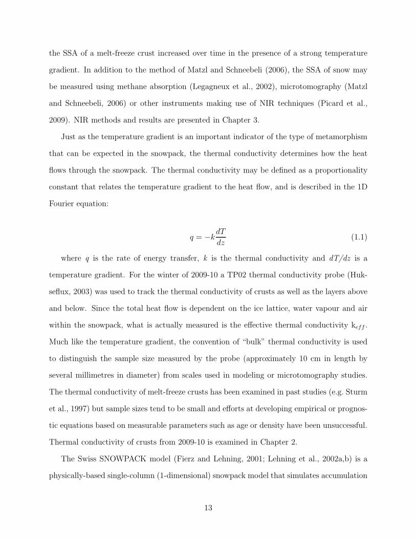
Just as the temperature gradient is an important indicator of the type of metamorphism
that can be expected in the snowpack, the thermal conductivity determines how the heat
flows through the snowpack. The thermal conductivity may be defined as a proportionality
constant that relates the temperature gradient to the heat flow, and is described in the 1D
Fourier equation:
q = −kdT
dz(1.1)
where q is the rate of energy transfer, k is the thermal conductivity and dT/dz is a
temperature gradient. For the winter of 2009-10 a TP02 thermal conductivity probe (Huk-
seflux, 2003) was used to track the thermal conductivity of crusts as well as the layers above
and below. Since the total heat flow is dependent on the ice lattice, water vapour and air
within the snowpack, what is actually measured is the effective thermal conductivity keff .
Much like the temperature gradient, the convention of “bulk” thermal conductivity is used
to distinguish the sample size measured by the probe (approximately 10 cm in length by
several millimetres in diameter) from scales used in modeling or microtomography studies.
The thermal conductivity of melt-freeze crusts has been examined in past studies (e.g. Sturm
et al., 1997) but sample sizes tend to be small and efforts at developing empirical or prognos-
tic equations based on measurable parameters such as age or density have been unsuccessful.
Thermal conductivity of crusts from 2009-10 is examined in Chapter 2.
The Swiss SNOWPACK model (Fierz and Lehning, 2001; Lehning et al., 2002a,b) is a
physically-based single-column (1-dimensional) snowpack model that simulates accumulation
13

and metamorphism of snow. Simulations may be driven by measured or modeled (e.g.
Bellaire et al., 2011) meteorological data and may be initialized either while the ground is
bare or using an observed snow profile. Snow erosion and transport are included through the
option to simulate slopes and the model has been used operationally or tested by avalanche
forecasters in Switzerland, Canada and Japan (Hirashima et al., 2008). Due to its single-
column nature it is not suitable for simulating layers that are spatially variable on the
scale of a single slope (Smith et al., 2008). SNOWPACK version 3.2, released in February
2014, was used to simulate natural crusts in the Mount Fidelity permanent closure area of
Glacier National Park. Output data were compared to observations of layer depth, hardness,
temperature, SSA and, for winter 2009-10, thermal conductivity measurements. The model,
methods and results are given in Chapter 4.
Field observations were collected over the course of three winters at fixed study plots in
Glacier National Park, in the Columbia Mountains of British Columbia, Canada. Methods
were specified by the author and were carried out by the author and other members of the
The Applied Snow and Avalanche Research group at the University of Calgary (ASARC)
research team, with the author present at all but one site visit. Methods such as the snow
profile conformed to standards specified in CAA (2007) with more detail within and around
target crusts. NIR photography was adapted from methods described by Matzl and Schnee-
beli (2006), and thermal conductivity measurements were done in accordance with man-
ufacturer’s recommendations (Hukseflux, 2003) modified slightly after testing to determine
appropriate methods and power sources for use in the field. Methods for cold lab experiments
were adapted from those described in Jamieson and van Herwijnen (2002), with varied mea-
surement intervals and experiment lengths to account for the limited number of observations
that could be taken from the insulated sample box.
NIR photographs were examined weekly to ensure that the camera equipment was func-
tioning properly, as well as to check for contamination of the Spectralon standards. Thermal
14
conductivity data were processed weekly and checked for consistency in heating power of the
TP02 and validity of sample data. All post-season processing and analysis were done by the
author.
SNOWPACK simulations were designed and run by the author following recommenda-
tions by the model’s developers as well as by other members of the ASARC research team.
Input meteorological data were quality-controlled from ASARC and Parks Canada instru-
mentation at Mount Fidelity study area. In the cases where simulations were not started
with bare ground, input snow files were built by the author using ASARC and Parks Canada
profiles as sources. Snow profile data used for validation of model output were recorded by
ASARC and Parks Canada. All analysis of model output was conducted by the author.
Results from Chapters 2-4 are synthesized in Chapter 5 and recommendations for future
research are given in Chapter 6. A glossary is included in Appendix B as an easy reference
for some terms used in this study.
15
Chapter 2
Thermal Conductivity
In this chapter the property of thermal conductivity is introduced along with how it may be
used to describe the structure of a snow sample. For the winter of 2009-2010 a heated needle
thermal conductivity probe was used to monitor changes in six natural crusts and five crusts
in the cold lab. It was also used to measure the spatial variability of thermal conductivity
at a crust site from the winter of 2008-09.
Students in professional avalanche courses in Canada are introduced to a document called
”Observational Guidelines and Recording Standards”, or OGRS for short (CAA, 2007).
OGRS describes in detail procedures for collecting and recording snowpack observations. It
is well written, succinct and extremely useful for communication observations amongst the
hundreds of avalanche professionals in Canada. Unfortunately there is no such document for
snow scientists who have long realized that describing the texture of snow, should they be
lucky enough to find a perfectly homogeneous layer, is exceedingly difficult when the goal is
to illuminate the relationships between structure and physical properties and processes.
The point of the preceding paragraph is to introduce the difficulty of describing snowpack
structure precisely, accurately and consistently. This becomes even more difficult when
attempting to quantify changes over time in the field and with multiple observers. At
present thermal conductivity is used exclusively for research, and not operational avalanche
forecasting purposes. Chapter 3 describes the use of near-infrared photography to objectively
describe the structure and spatial variation of the specific surface area of layers exposed on
a pit wall.
Overall these measurements were found to be quick and easy to conduct in both field and
lab-based studies. Some problems with free water and melting of samples were encountered
16

when the snowpack temperature was close to 0 ◦C and in layers with large icy inclusions.
2.1 Non-steady-state thermal conductivity theory
Thermal conductivity has long been recognized as an important physical parameter of the
seasonal snow as it directly influences changes in crystal habit, size and bonding and thus
affects everything from snowpack stability to heat exchange within climate models (e.g. Cook
et al., 2008). Thermal conductivity is most simply described by the 1D Fourier equation,
q = −kdT
dz(2.1)
where k is the thermal conductivity. Put into words, the thermal conductivity is a pro-
portionality constant that relates a gradient (in this case the vertical temperature gradient)
to the heat flow. The vertical temperature gradient is used here as it is traditionally mea-
sured by avalanche practitioners and it is usually much stronger than the gradient in the
horizontal directions. The convention used in this paper is that negative gradients mean
colder temperatures toward the snow’s surface. For scales of 10 cm to 1 m Equation 2.1 is
probably a reasonable approximation to the bulk heat transport, but at the polycrystalline
or grain scale things are not so simple due to the unequal distribution of pore space and
effects of thermal pathways (tortuosity) through the ice lattice. To further complicate the
matter, only in the thermal conductivity due to the ice lattice (klatt) or perhaps due to
the water vapour (kvap) may be of interest. In practice the two often cannot be measured
sseparately and instead the effective thermal conductivity, keff is measured. A semantic
distinction must be adopted here to avoid confusion: Unless otherwise specified, the terms
thermal conductivity, bulk thermal conductivity and effective thermal conductivity will be
used synonymously throughout this text. ’Bulk’ is used here to emphasize that samples are
taken at the macro scale, on the order of 10 centimetres. A number of studies introduced in
this chapter discuss thermal conductivity on the micro-scale, that is on the scale of microns
17

to millimetres. This distinction should further illustrate that thermal conductivity samples
are a complex function of the structure and bonding of the ice lattice, the temperature of
all three phases of water (if present), vapour pressure and time.
Sturm et al. (1997) divides thermal measurement conductivity techniques into 3 classes:
Fourier-type, steady-state and transient-flow, or non-steady-state (NSS). Fourier-type anal-
yses measure the thermal diffusivity and then determine the thermal conductivity through
monitoring of the phase shift of temperatures at different points throughout the sample
period. In this case the thermal diffusivity is the ratio of the thermal conductivity to the
density times the specific heat capacity.
Steady state techniques apply heat across a sample, but require that it come into thermal
equilibrium before a measurement is made. The guarded hot plate (e.g. Riche and Schneebeli,
2010) is an example of a steady state technique. Although accurate, it is cumbersome for
field use.
NSS techniques apply a temperature gradient to a sample but do not require thermal
equilibrium. The advantage of these techniques is the time and equipment required are
reduced compared to steady state techniques. The most common technique involves the use
of a heating wire which is treated as a perfect line heat source. Blackwell (1956) introduced
an equation for the relative error in making such an assumption and found that a solid heated
needle with a length/diameter ratio of 30 would give a maximum error of about 0.12%.
NSS techniques may be further classified into short-time (Britsow et al., 1994) and long
time approximations to the analytical solution. In the short-time case the contact resistance
between the probe and medium must be known. Riche and Schneebeli (2010) found that
contact resistance was strongly affected by the insertion of the needle probe and resulted
in thermal conductivities of 2-3 times less than those measured using a guarded hot plate
apparatus. In the long-time case after a certain transient period the rate of temperature
increase becomes constant and no longer depends on the probe’s thermal properties and
18
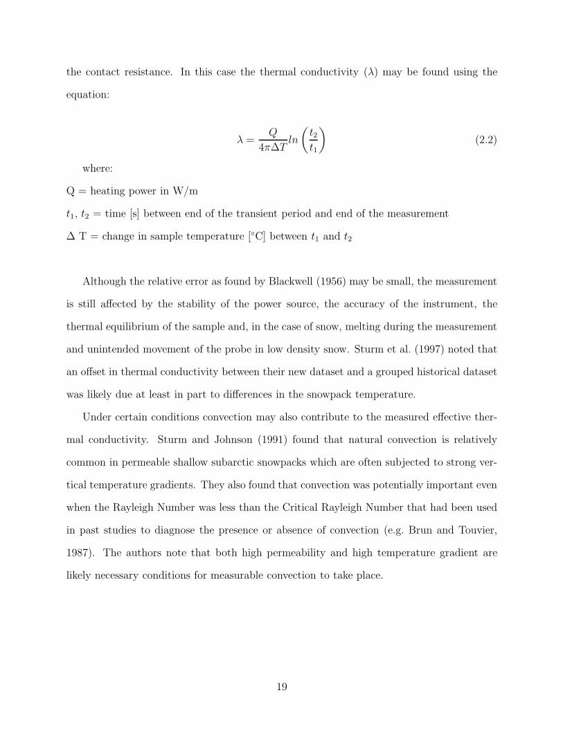
the contact resistance. In this case the thermal conductivity (λ) may be found using the
equation:
λ =Q
4π∆Tln
(
t2
t1
)
(2.2)
where:
Q = heating power in W/m
t1, t2 = time [s] between end of the transient period and end of the measurement
∆ T = change in sample temperature [◦C] between t1 and t2
Although the relative error as found by Blackwell (1956) may be small, the measurement
is still affected by the stability of the power source, the accuracy of the instrument, the
thermal equilibrium of the sample and, in the case of snow, melting during the measurement
and unintended movement of the probe in low density snow. Sturm et al. (1997) noted that
an offset in thermal conductivity between their new dataset and a grouped historical dataset
was likely due at least in part to differences in the snowpack temperature.
Under certain conditions convection may also contribute to the measured effective ther-
mal conductivity. Sturm and Johnson (1991) found that natural convection is relatively
common in permeable shallow subarctic snowpacks which are often subjected to strong ver-
tical temperature gradients. They also found that convection was potentially important even
when the Rayleigh Number was less than the Critical Rayleigh Number that had been used
in past studies to diagnose the presence or absence of convection (e.g. Brun and Touvier,
1987). The authors note that both high permeability and high temperature gradient are
likely necessary conditions for measurable convection to take place.
19

2.2 Past Measurements
Studies dating to at least 1886 (Sturm et al., 1997) have attempted to measure the thermal
conductivity of snow. The techniques and accuracy are varied but in general most efforts
prior to 1950 employed some form of Fourier analysis to derive the thermal conductivity
of a bulk sample. In recent years advances in instrumentation have simplified the task of
collecting thermal conductivity measurements in the field, with most recent field studies
making use of heated needle probes.
Sturm et al. (1997) summarize 26 studies conducted between 1886 and 1991 in what
remains the definitive compilation of snow thermal conductivity data. Mean values in their
data set ranged from 0.131 W m−1K−1 for samples with a mean density of 222 Kgm−3 to
0.810 W m−1K−1 for samples with a mean density 496 Kgm−3. They note that although
many studies have published relationships between density and thermal conductivity, the
combined historical dataset shows no such relationship. Furthermore, the relationship be-
tween temperature and thermal conductivity was generally ignored in most studies. They
and others (Arons, 1994) also emphasize the temperature dependence of the effective thermal
conductivity of snow which, at least according to theory, becomes pronounced between -20
◦C to 0 ◦C.
The same paper introduced a new set of measurements which added to the the authors’
previous work (see Sturm and Johnson, 1992). All thermal conductivity data were collected
using an instrument similar to that described in Section 2.4. This is the first dataset where
samples are described by their International Classification for Seasonal Snow on the Ground
(Colbeck et al., 1992; Fierz et al., 2009), allowing a more direct comparison with the crusts
which are the target of the present study: Samples of refrozen grains had thermal conductiv-
ities of 0.095 W m−1K−1 to 0.250 W m−1K−1 for densities ranging from 314 Kgm−3 to 496
Kgm−3 though this group also had the largest standard deviation in thermal conductivity
of all grain types.
20

Relationships between density and thermal conductivity based on grain type were also
introduced: For “density independent” snow types (depth hoar and other faceted types), the
use of a single mean value was found to give the best fit to the measurements. For other
types, both quadratic fits and maximum likelihood estimator were proposed. A follow-up
study by Sturm et al. (2002) found good agreement with the above regressions when used
to predict the thermal conductivity of layers classified by hand hardness and density.
Riche and Schneebeli (2010), in addition to evaluating the accuracy of short-time heated
needle probes, used a guarded heat plate to measure thermal conductivities between 0.151
(ρ = 213 Kgm−3) and 0.185 W m−1K−1 (ρ = 239 Kgm−3) for rounded grains.
Schneebeli and Sokratov (2004) applied vertical temperature gradients to sieved snow
samples and used microtomography to track structural changes as they underwent metamor-
phism. They observed an initial sharp increase in thermal conductivity from approximately
0.35 to 0.55 W m−1K−1 for samples with a constant density of 500 Kgm−3 while lower
density samples tended to remain constant around their initial value of 0.11 W m−1K−1.
Satyawali et al. (2008) applied high vertical temperature gradients (28 ◦C m−1) to sifted
natural snow samples and monitored microstructural and thermophysical changes over a
period of 4 weeks. They noted that the thermal conductivity in samples with an initial
density of ρ = 180 Kgm−3 increased more quickly during the 4 weeks and to ultimately
higher values than another sample with initial density ρ = 320 Kgm−3. The pore intercept
length also increased more quickly in the low density sample. This increase in thermal
conductivity coupled with only a small increase in density implies that the ice skeleton in
low density snow may rearrange itself into effective pathways for heat conduction faster
than similar snow of higher density. A similar conclusion was drawn by Sturm and Johnson
(1992) with respect to depth hoar in a shallow, highly faceted snowpack. This relationship
between initial density and rate of change of thermal conductivity is opposite that observed
by Schneebeli and Sokratov (2004) and may be due to similar factors that led Sturm et al.
21

Table 2.1: A summary of published values of snow thermal conductivity since 1997. Thegrains in Satyawali 2008 were subjected to a high temperature gradient, but started as roundedgrains (RG).
Study λ [Wm−1K−1] Grain ρ [Kgm−3] Tmean [◦C]Sturm 1997 0.095-0.445 MFcl 314-496 -10.8Sturm 1997 0.099-0.218 FCxr/RGxf 280-416 -12.1Sturm 1997 0.021-0.142 DHch 154-369 -14.4Sturm 1997 0.051-0.632 RGsr 170-340 -12.9Schneebeli 2004 0.10-0.12 RG 260-300 -8
Satyawali 2008 0.10-0.12 RG (initial) 320 -7.2
Satyawali 2008 0.09-0.17 RG (initial) 180-200 -7.3Riche 2010 0.073,0.061 RG 213,239 -15
Courville 2007 0.29 (mean) RGwp 400 -25 to -40Courville 2007 0.15 (mean) FC (firn) 400-500 -25 to -40
Sturm 1997 0.022 - 0.024 Air 1 -20 to 0
Sturm 1997 2.2 - 0.0 Ice 917 -20 to 0
Singh 2009 0.3 - 0.4 MF 480 -30 to -5
(1997) to conclude that density is not a good predictor for thermal conductivity in faceted
grain types. Calonne et al. (2011) and Greene (2007) also observed the formation of highly
faceted grain types with no attendant change in density.
A summary of published values of thermal conductivity is shown in Table 2.1. Grain
types are those defined in Fierz et al. (2009).
2.3 Modeling
Many efforts at modelling prior to the late 1990s were hindered by the absence of information
on the true microstructure of a snow sample. Although stereology could be used to estimate
parameters such as connectivity and intercept length there was no way of simulating heat
transport through the true structure of a snow sample. Modelers were thus constrained to
using combinations of idealized shapes to simulate heat transfer through the lattice. Colbeck
(1983) achieved some success in modelling crystal growth rates in dry snow but concluded
the ”the fact that we had to assume a distribution [for a geometrical enhancement factor]
22

points out the need for stereographic work on snow at various stages of metamorphism.”.
Arons and Colbeck (1995) summarized a number of efforts at physically-based snowpack
modeling and reached a similar conclusion to Colbeck, while emphasizing the importance of
texture, anisotropy and scale to heat transport in snow.
Adams and Sato (1993) developed a 1-D analytic model for the effective thermal con-
ductivity of an isotropic snow sample represented by a collection of spheres, where heat was
allowed to travel through either pore space, ice or pore space and ice in series. They found
that the thermal conductivity was dominated by the ratio of bond radius to grain radius as
well as the coordination number (degree of interconnectedness) and explained qualitatively
a potential feedback mechanism for the growth of depth hoar.
The model of Adams and Sato (1993) was incorporated into the 1-dimensional SNOW-
PACK model (Bartelt and Lehning, 2002). SNOWPACK is a physically based model for
metamorphism in the seasonal snow. See Chapter 4 for more detail on the model. The ther-
mal conductivity in SNOWPACK is solved at discrete timesteps based on a layer’s physical
and microstructural properties. Fierz and Lehning (2001) found good qualitative agreement
between SNOWPACK and measured thermal conductivities while at the same time conclud-
ing that the single adjustable parameter of neck to bond radius, even when combined with
density is not adequate for the variety of textures that may be found in snow of similar
densities. A study by Greene (2007) showed that while SNOWPACK consistently predicted
thermal conductivity to within 10% of its measured value, it did not satisfy the criteria for
‘model skill’ outlined by Pielke (2002), that the standard deviation of modeled values be
approximately equal to the standard deviation of the observed values and; the root mean
squared error (RMSE) and RMSE with constant bias removed be smaller than the standard
deviation of the observed values. Jamieson and Fierz (2004) used the model to approximate
freezing times in a buried wet layer and found good agreement with measured data although
thermal conductivity was not explicitly evaluated.
23
Bartelt et al. (2004) modified the model of Adams and Sato (1993) with the addition of a
radiative transfer term to the ice thermal conductivity equation, though it was still confined
to one dimension and a single neck to bond ratio for each layer. The new model was used in
a modified formulation of the SNOWPACK model that allowed ice and pore space to be out
of thermal equilibrium. Simulations showed that heat transfer through the ice/pore interface
is potentially important, and that physical models should account for this by treating ice
and air phases separately when calculating the bulk thermal conductivity. The utility of
this new non-equilibrium model lies as much in distancing physically based models from
empirical formulations as it does in calculating point values of thermal conductivity.
Satyawali and Singh (2008) explored the role of grain shape in explaining the the wide
scatter apparent in previous measurements of thermal conductivity versus density. Their
model results assumed constant thermal conductivity for ice and showed a clear dependence
of bulk thermal conductivity on shape, with the highest conductivities found in layers with
good bonding and spherical shapes and the lowest for cubic shapes with poor bonding.
Their approach offers a promising compromise between having complete 3-D microstructural
information and usability given the current state of knowledge.
Singh and Wasankar (2009) used the contiguity of snow (the fraction of a given phase in
contact with another phase) to define the contact between adjacent phases, along with den-
dricity and sphericity, which together can be used to define the degree of metamorphism from
new snow to either rounded or faceted forms. Their model showed relatively good agreement
with thermal conductivity measurements from a high density melt-freeze crusts whose mi-
crostructural parameters were defined using image analysis software. A more comprehensive
comparison is not possible as their microstructural parameters were not published.
Kaempfer et al. (2005) used computed X-ray micro-tomography to study heat transport
in snow. A snow sample was subjected to a temperature gradient and was simultaneously
imaged for use in a finite element model. Simulations neglecting any heat flow through pore
24

space resulted in thermal conductivity values that were approximately 80% of measured
values implying that most heat flow is through the ice lattice. Similar to Bartelt et al.
(2004), their simulations found high temperature gradients concentrated in small grain-scale
regions. Consideration of the sample’s tortuosity shows that idealized samples consisting
of spheres and with tortuosities of 2.0-2.1 don’t alter the path of heat flow relative to the
axis of vapor diffusion, whereas a real snow sample with a tortuosity of 4.4±0.3 forces it
to travel along a much more sinuous path which, given the relatively higher conductivity of
the ice lattice, may lead to localized high temperature gradients at scales not measurable by
conventional methods.
Shertzter et al. (2010) introduced a 3-dimensional contact tensor to model the the change
in thermal conductivity through the ice skeleton as an isotropic snow sample subjected to a
vertical temperature gradient becomes anisotropic, with preferential bonding and increased
thermal conductivity developing in the direction of gradient. As with Kaempfer et al. (2005),
the contributions of conduction through air, convection and latent heat are ignored. The
model as presented was limited by its assumption of stationarity of all microstructural prop-
erties except for the contact tensor and could not be used to effectively model changes over
long periods but represents a promising start to incorporating more realistic microstructure
into snowpack models. Riche and Schneebeli (2013) studied the anisotropy of thermal con-
ductivity using heated needle probes and numerical simulations and found that, depending
on grain type, the effective thermal conductivity measured only in the horizontal plane can
lead to errors of up to 25%.
Kaempfer and Plapp (2007) and Kaempfer et al. (2009) built on previous µ-CT modelling
efforts by using a phase field to represent the air-ice interface. Models of heat flow in two
dimensions showed clearly the preferred pathways through oriented bonds but also allowed
the contribution of air and water vapour, though convection was still neglected. Some sim-
plifications were required in order to reduce computational time and no quantitative results
25

were obtained; however, the method shows qualitatively how heat flow and snow metamor-
phism may effectively be modeled using physical laws and real microstructure. Calonne et al.
(2011) modeled the thermal conductivity of snow samples in three dimensions using µ-CT
images and found significant anisotropy between the vertical and horizontal planes, though
their model only considered conduction through the ice lattice and interstitial air.
Finally, although they are not explicitly applicable to the present study, much larger-scale
models also depend on accurate characterization of snow’s thermal conductivity. Cook et al.
(2008) studied the sensitivity of a model to a range of conductivities and found measurable
differences in heat exchange with the lower atmosphere as well as soil temperatures and
permafrost dynamics.
Although there is a growing body of research regarding the thermal conductivity of
natural snow there has been very little research devoted to an understanding of changes over
time of specific snowpack layers, especially melt-freeze forms. Part of the goal of the current
study is to fill this gap in the knowledge and synthesize results with concurrent observations
of structure, density, temperature, grain form and specific surface area. The remainder of
this chapter deals exclusively with observations of thermal conductivity. Results from this
and other chapters are summarized together in Chapter 5.
2.4 Equipment
A Hukseflux TP02 thermal non-steady-state thermal conductivity probe (Hukseflux, 2003)
was used for all measurements in this study. The probe, shown schematically in Figure
2.1, is designed to be used with the long-time approximation given in Equation 2.2. This
means that incidences of poor contact between the probe and the sample will simply take
longer to transition out of the zone of transient temperature increase. The power to the
heating wire was controlled by a resistor in series from the 12 V power source and was
measured with the use of a 10 Ohm 0.1% resistor. A thermistor in the base of the probe
26

Figure 2.1: Schematic of the Hukseflux TP02 thermal conductivity probe. Adapted fromFigure 1 in Hukseflux (2003)
gives a reference temperature and enables a direct calculation of the thermal conductivity.
The manufacturer’s stated accuracy at 20◦C is ± (3% + 0.02) W m−1K−1. A correction
during post-processing limits the error due to temperature to ± 0.02%, but measurements of
low thermal conductivity will still have relatively high uncertainty due to the instrument’s
accuracy. Morin et al. (2010) modeled heat flow around the TP02 and found that the area
sampled extends approximately 3 cm radially from the probe.
The TP02 was paired with a Campbell Scientific CR10X datalogger. Several 12 V power
sources were tested including 6 V lantern batteries in series, 1.5 V AA batteries in series
and an AC-to-12 V inverter. Ultimately the most stable power source was from the AA
batteries and these were used for the majority of measurements in the field. All data were
recorded at 1 second intervals for quality control during post-processing. The logger program
also had several built-in warnings for unstable sample temperature heater power for real-
time evaluation of measurement quality. An Ipaq 3950 hand-held computer and Campbell
Scientific PConnectCE software were used to trigger TP02 measurements and monitor values
as the measurement progressed.
The TP02 probe was new at the beginning of the 2009 - 2010 and came factory cali-
brated. No further calibrations were performed. Prior to use in the field all connections
and resistances in the probe were verified to be within tolerances specified by Hukseflux.
Connections with the CR10X datalogger were checked before each use.
27

2.5 Field Methods
The majority of TP02 data were gathered in the field simultaneously with other snowpack
measurements. A test snow profile was used to describe qualitatively the crust structure
and spatial variability over the scale of the pit wall (approximately 1 m horizontally). Near-
infrared photography (Chapter 3) was used to record quantitative information on structure
and variability.
Once the complementary measurements were completed, the TP02 was inserted into
the layer of interest for several minutes to allow it to reach thermal equilibrium with the
surrounding snowpack. This was checked by comparing the TP02’s thermistor temperature
with the layer temperature previously measured as part of the snow profile.
Once the measurement was triggered the probe temperature was allowed to stabilize for
an additional 100 seconds before starting a 100-second heating cycle. Similar procedures
were used by Morin et al. (2010) and Domine et al. (2012). The probe tip temperature
was monitored to ensure that the temperature increase did not exceed 1.0 ◦C. Occasional
problems were encountered at low temperatures when the stiff probe cable made it difficult
to prevent the probe from shifting out of the sample area. These measurements were always
discarded. Excepting cases where the crust was too warm, a minimum of two valid measure-
ments were attempted for each layer. Typically the layer above (samples 1 and 2 in Figure
2.2, layer below (samples 5 and 6) and one or more layers within the crust itself (samples
3, 4, 7 and 8) were sampled. A final NIR image was then taken to record the position of
each sample. NIR images were found to be superior to visible images for resolving layers
and variability within the wall of a snow pit. An example is shown in Figure 2.2
In addition to field measurements, five cold lab experiments, similar to those conducted
by Jamieson and Fierz (2004), were conducted to observe changes in and around a wet crust
as it froze. Thermal conductivity measurements followed a similar procedure as for field
measurements except that measurements were taken vertically through the crust. Care was
28

Figure 2.2: Annotated NIR photograph of TP02 sampling locations. Layer boundaries andsampling locations are more easily discerned in this NIR photo than in photographs takenwith a conventional digital camera in the visual spectrum. Similar images were used tocomplement field notes regarding depth of sampled layers and layer homogeneity.
29
taken to ensure that the thermistor, thermocouples and heating portion of the wire were
always positioned the same relative to the the layers of interest. Cold lab crusts all had
thickness greater than 10 cm thus ensuring that no portion of the probe was sampling an
adjacent layer.
Although the majority of measurements were successful there were a number of challenges
encountered. The winter of 2009 - 2010 was abnormally warm and dry (see Appendix A)
and as a consequence layers were often very close to 0 ◦C. Very faceted and disaggregated
layers also proved difficult to sample due to large voids or extreme variability. Crusts were
occasionally difficult to penetrate with the probe due to icy inclusions.
Power presented a minor challenge as the TP02 requires a stable source of 12 VDC power.
Analysis of initial results found that nine 1.5 V rechargeable batteries were more stable, even
at cooler temperatures, than two 6 V lantern batteries in series. Somewhat surprisingly, the
AC power available in the Rogers Pass cold lab was the least stable of all power sources and
was not used after the initial cold lab experiment on March 12, 2010.
2.6 Results and Analysis
A total of 261 successful thermal conductivity measurements were recorded in the field and
in the lab during the study period. Although melt-freeze crusts were of greatest interest the
layers above and below were also sampled. Table 2.2 summarizes the thermal conductivity
measurements for each study site and cold lab experiment. Refer to Appendix A for locations
and summaries of crust formation.
The analysis in this section is divided into several parts: In Section 2.6.1 thermal con-
ductivity by grain type is summarized and compared with previous studies; in Section 2.6.2
links between thermal conductivity and physical characteristics of the sampled layers are
investigated. This is similar to analyses performed in the past by Sturm et al. (1997), Sturm
and Johnson (1992) and Kaempfer et al. (2005) and to the author’s knowledge is the first
30

Table 2.2: Observation period and number of thermal conductivity measurements duringwinter 2009-10. Crusts are named by geographical location and month/day of initial burial.BV: Beaver Valley; FI: Mt Fidelity; SR: South Run; RP: Rogers Pass study plot; LAB:Rogers Pass cold lab.
Crust Name Start End Num. site visits Approx. intervalBV0112 01/31 03/23 7 weeklyFI0109 01/10 04/14 14 weeklyFI0308 03/15 04/14 5 weeklyRP0112 01/19 04/06 11 weeklySR0131 02/03 04/07 10 weeklySR0210 02/03 04/07 9 weeklySR09 02/05 02/05 11 spatial samples OnceLAB0312 03/12 12:00 03/13 15:10 7 30 minLAB0330 03/30 09:30 03/30 12:05 3 hourlyLAB0409 04/09 13:00 04/10 14:30 5 6 hoursLAB0410 04/10 19:15 04/13 09:35 6 twice dailyLAB0413 04/13 04/18 6 daily
performed in a transitional snow climate. In Section 2.6.3 changes over time in thermal
conductivity are examined along with its relationship to rates of change in other physical
parameters. These are compared with a number of past studies that have either tracked
physical changes or modeled changes over time. Section 2.6.4 gives a brief look at some of
the difficulties in selecting a site for tracking temporal changes in buried layers.
All thermal conductivity measurements, both successful and unsuccessful, are given in
Appendix C. The high incidence of bad measurements late in the season was due primarily
to the layer of interest being at or near 0 ◦C.
Determination of the quality of each measurement was done manually in Microsoft Excel.
Although the CR10X program included automated checks for quality, they frequently failed
to identify bad measurements and incorrectly flagged good measurements. An ideal mea-
surement will begin with a short period of transient heating before the rate of temperature
31

increase becomes constant. For a constant heating power Q, Equation 2.2 becomes:
λ =Constant
∆Tln
(
t2
t1
)
(2.3)
where t1 is the time, in seconds, at which the rate of increase of the sample temperature
becomes constant, t2 is the end of the measurement period and ∆T is the nominal rise in
temperature between the two points. The term ‘nominal‘ is used because the increase in
temperature is relative to the temperature of a thermocouple at the base of the TP02, which
serves to compensate of any changes in the layer temperature during measurement. This
zone of constant temperature increase is linear when plotted using the natural logarithm of
the ratio of t1 and t2 and is thus well suited for graphical analysis. Figure 2.3 shows a typical
plot of nominal temperature rise versus ln(t). The value of λ is found by taking the inverse
of the slope of the best-fit dashed line.
Concerns regarding the accuracy of heated needle probes were raised by Riche and Schnee-
beli (2010), who found that the needle is potentially in contact with only a small number
of grains along its length. This concern was addressed by Morin et al. (2010) who modeled
these effects and found that the only consequence would be a slight delay in the measurement
reaching a rate of constant temperature increase.
Upper and lower limits for plausible values of λ may be estimated by using the thermal
conductivities of pure ice and air. Ashton (1986) gives the following equation for pure ice
valid from -40 to -0.1 ◦C.
λ = 2.21− 0.011T (2.4)
The majority of measurements were taken at temperatures warmer than -10 ◦C so fol-
lowing Equation 2.4 our limits for plausible thermal conductivity of snow and ice become
0.025 ≤ λ ≤ 2.32 Wm−1K−1, where the lower limit is the approximate thermal conductivity
of air and the upper limit is the thermal conductivity of pure ice.
32

Figure 2.3: A typical plot of ln(t) versus the nominal rise in temperature. The thermalconductivity is the inverse of the slope. In this plot the slope is 8, so λ is approximately0.125 [Wm−1K−1]
2.6.1 Thermal conductivity by grain type
Table 2.3 shows the summary statistics for thermal conductivity measurements by grain
type. There were enough instances of mixed faceted (FC) and melt-form (MF) layers that a
new classification denoted ’MFFC’ was created from the MF subset of grains. These layers
were often spatially variable on the scale of the needle probe and multiple grain types were
likely included in each thermal conductivity measurement. This decision may be tested using
a Mann-Whitney U-test: With no removal of outliers the null hypothesis (at p ≤ 0.10) that
the distributions of thermal conductivity for MF and MFFC are the same is rejected.
The range of valid measurements is very similar to the theoretical limits calculated using
Equation 2.4. The two subgroups of melt forms have substantially different mean thermal
conductivity and density suggesting that this discrimination is worthwhile. As might be
expected, ice forms (IF) have the highest mean thermal conductivity while precipitation
particles (PP) have the smallest values.
33

Table 2.3: Thermal conductivity and density by grain type. Units for thermal conductivityare [Wm−1K−1]. MF* and MFFC denote two subgroups of melt-forms (MF)
Grain # Valid λ σλ λMAX λMIN ρ [Kgm−3] # Valid ρ
ALL 261 0.205 0.200 2.103 0.022 279 190MF 112 0.203 0.216 2.103 0.025 289 58MF* 103 0.210 0.224 2.103 0.025 304 49MFFC 9 0.127 0.052 0.236 0.064 210 9FC 96 0.204 0.206 1.727 0.044 285 95PP 5 0.068 0.028 0.108 0.040 89 6RG 26 0.213 0.115 0.553 0.042 299 26IF 10 0.317 0.196 0.843 0.175 NA 0DF 6 0.090 0.036 0.122 0.090 145 6
Distributions for each grain type were tested for normality using the Shapiro-Wilk Nor-
mality test. The null hypothesis of normality for all grain types was rejected based on the
presence of a small number of outliers in each data set. A series of kernel density plots
showed large right-hand tails for most grain types due to a relatively small number of high
values. Density plots for each grain type reveal similar tails except for types with few sam-
ples (MFFC and PP) and rounded grains (RG) which hints at a mixed-mode distribution.
Further investigation reveals that two samples from a relatively high-density layer late in
the season are likely responsible.
Given the probable presence of outliers, there is value in probing further into measure-
ments that may not be representative of the larger population. The definition of what exactly
constitutes an outlier is subject to debate and depends on a number of factors including a
priori knowledge of the expected distribution. Outliers are defined here as any values further
than 1.5 times the interquartile range from the upper and lower quartiles.
Figure 2.4 shows a box-whisker plot of all thermal conductivity measurements by grain
type. The labels ‘MFFC‘ and ‘MF‘ correspond to the summary stats for groups MF* and
MFFC in Table 2.3. Outliers are circled in red. MF* and FC have the greatest number of
outliers while MFFC and PP have none.
34
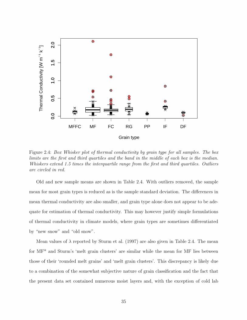
0.0
0.5
1.0
1.5
2.0
Grain type
The
rmal
Con
duct
ivity
[W m
−1 k
−1 ]
0.0
0.5
1.0
1.5
2.0
MFFC MF FC RG PP IF DF
Figure 2.4: Box Whisker plot of thermal conductivity by grain type for all samples. The boxlimits are the first and third quartiles and the band in the middle of each box is the median.Whiskers extend 1.5 times the interquartile range from the first and third quartiles. Outliersare circled in red.
Old and new sample means are shown in Table 2.4. With outliers removed, the sample
mean for most grain types is reduced as is the sample standard deviation. The differences in
mean thermal conductivity are also smaller, and grain type alone does not appear to be ade-
quate for estimation of thermal conductivity. This may however justify simple formulations
of thermal conductivity in climate models, where grain types are sometimes differentiated
by “new snow” and “old snow”.
Mean values of λ reported by Sturm et al. (1997) are also given in Table 2.4. The mean
for MF* and Sturm’s ‘melt grain clusters’ are similar while the mean for MF lies between
those of their ‘rounded melt grains’ and ‘melt grain clusters’. This discrepancy is likely due
to a combination of the somewhat subjective nature of grain classification and the fact that
the present data set contained numerous moist layers and, with the exception of cold lab
35

Table 2.4: Thermal conductivity by grain type with and without outliers, compared with thosereported by Sturm et al. (1997).
Grain λ λ outliers removed # outliers λ Sturm Sturm97 grainALL 0.204 0.170 13MF 0.203 0.173 4 0.188 rounded melt grainsMF* 0.210 0.177 4 0.250 melt grain clustersMFFC 0.127 0.127 0FC 0.204 0.165 6 0.153 mixed formsRG 0.213 0.187 2 0.169 small rounded grainsPP 0.068 0.068 0 0.070 new snowIF 0.317 0.239 2DF 0.076 0.094 1 0.128 recent snow
crusts all samples were taken at much warmer temperatures. Referring back to Tables 2.3
and 2.1, the values published by Singh and Wasankar (2009) for MF are slightly greater than
our mean λ but were also taken from layers with a higher density. The mean value for RG
is larger than Sturm’s and much greater than those published by Schneebeli and Sokratov
(2004), Satyawali and Singh (2008) and Riche and Schneebeli (2010) for layers of similar
density; however, the range of measurements is similar to Sturm’s.
The three largest values for FC come from three different sites and all layers were recorded
as being moist. Pure water has a thermal conductivity of approximately 0.563 Wm−1K−1
at 0 ◦C and it’s likely that the presence of free water in the ice lattice affects λ, although
without knowing precisely the water content it is not possible to quantify the contribution.
Given the heterogeneous structure of many crusts, the observation of some high thermal
conductivities in MF forms is not surprising. The four outliers come from three different
sites: Two were vertical measurements through the crust and two were measured parallel to
the layer plane. None of the subjective observations (hand hardness, moisture content) or
quantitative (layer temperature, density) set them apart from other samples.
Outliers aside, the distribution of MF observations does not appear normal and it is
worth searching for any trends in seasonality or site. No trends in seasonality were found,
36

Table 2.5: Thermal conductivity for crust samples (MF) by site. Units for thermal conduc-tivity are [Wm−1K−1]. The final column gives the mean with outliers removed.
Site # Valid λ λ λMAX λMIN σλ # outliers λ*BV0112 10 0.181 0.193 0.317 0.062 0.085 0 0.181FI0308 16 0.324 0.184 2.100 0.055 0.486 3 0.191FI0110 12 0.298 0.240 0.843 0.175 0.183 2 0.232RP0112 25 0.142 0.135 0.239 0.059 0.0534 0 0.142SR0131 8 0.226 0.153 0.714 0.055 0.210 1 0.156SR0210 7 0.126 0.134 0.225 0.028 0.073 0 0.126LAB0312 5 0.259 0.142 0.648 0.089 0.228 1 0.162LAB0330 9 0.170 0.193 0.285 0.035 0.092 0 0.170LAB0409 7 0.262 0.252 0.690 0.072 0.206 1 0.191LAB0410 11 0.213 0.246 0.409 0.025 0.117 0 0.213LAB0413 10 0.244 0.251 0.414 0.081 0.100 0 0.244
however individual sites did differ. Table 2.5 shows summary statistics for MF crusts at each
site. Several sites stand out as having appreciably greater means than others. These are
explained at least in part by high outlying values for sites FI0308 and RP0112, but even with
the removal of outliers the cold lab experiments appear to have higher mean values than the
field sites. There are two possible reasons for this: The final three cold lab experiments used
crusts harvested from the same spot so it may be that this crust simply has a greater thermal
conductivity. A second possibility is the method used to measure the thermal conductivity.
Due to space constraints in the cold lab, the physical size of the harvested crusts had to
be small and thermal conductivity was measured vertically through the crust rather than
horizontally.
We use the Mann-Whitney U-test twice: Once to test whether field and lab thermal
conductivities come from different distributions and once to test the vertical and horizontal
measurements. In both cases the null hypothesis that the distributions are the same at the p
≤ 0.05 significance level is rejected. Unfortunately there is not a single site with concurrent
vertical and horizontal measurements throughout the entire season and no conclusions may
be drawn beyond the fact that the distributions are different.
37

Subsection 2.6.1 Summary In this section the relationship between thermal conductivity and
grain type has been examined. The majority of samples in this study were comprised of either
melt-freeze crusts or facets. Melt-freeze types were further divided into layers containing
transitional grain forms and those comprised purely of melt-freeze forms. Model distributions
for all grain types would have been approximately normal except for their large right-hand
tails. Removal of outliers gave the expected result of lower mean thermal conductivities and
standard deviations within each sample set, but also reduced the differences between grain
types.
The subset of MF samples was further analyzed to find temporal trends or differences
between sites. The cold lab experiments, with the exception of LAB0330, were found to
have different means than the field sites. This was due to either the fact that cold lab crusts
were harvested from the same location, or that thermal conductivity was measured vertically
through the crusts and parallel to the temperature gradient, while field sites were primarily
sampled parallel to the layer.
Thermal conductivity by grain type was compared to other published values where den-
sity and temperature information were available. When outliers were removed (in essence
removing most of the moist samples) the means for most grain types were similar to those
published by Sturm et al. (1997). Since many of the outliers were from moist layers this
highlights a potentially important distinction. When available, the ranges for λ for each
grain type were also similar across many of the studies.
The large range of measurements for each grain and the correspondingly large standard
deviations serve to reinforce the conclusion the grain type alone is not a sufficient predictor of
thermal conductivity. Given that many of the outliers were from layers identified as ‘moist’
or with temperatures near 0 ◦C, the qualitative measure of moisture content, commonly used
in test profiles and snow pits, does appear to be a useful distinction for any predicted value
of thermal conductivity even if no statistically significant relationships are found. The next
38

section explores the correlations between thermal conductivity, layer moisture, density and
layer temperature.
2.6.2 Thermal conductivity and physical parameters
The previous subsection examined the relationship between thermal conductivity and grain
type, including the distribution of measurements and the identification of possible outliers.
Results indicated that with the possible exception of coarse weather and climate models,
grain type alone should not be used to predict thermal conductivity. In this section the
relationship between thermal conductivity and density and layer temperature is analysed.
Figure 2.5 shows a scatter plot of λ and density for all grain types given in Table 2.3
except for ice forms (IF) which lacked density measurements. Thermal conductivity generally
increases with increasing density, but so does the heteroscedasticity. Outliers, circled in red,
are identified using the quantile method discussed in the previous section. The majority of
outliers are from samples that were moist. The empirical quadratic fit from Equation 4 in
Sturm et al. (1997):
λ = 0.138− 1.01ρ+ 3.233ρ2 (0.156 ≤ ρ ≤ 0.6)
λ = 0.023 + 0.234ρ (ρ < 0.156)
(2.5)
and logarithmic fit with a maximum likelihood estimator (MLE) correction given from Sturm
et al. (1997) Equation 7:
λ = 10(2.650ρ−1.652) (ρ ≤ 0.6) (2.6)
are plotted on each figure (where ρ has units of g cm−3), along with the quadratic fit from
Calonne et al. (2011):
λ = 2.5e−6ρ2 − 1.23e−4ρ+ 0.024 (2.7)
39

where ρ has units of kg m−3. Both equations were fit to data gathered using similar equipment
and methods to this study, albeit at colder temperatures. Both equations fit relatively well
to the trends in this study’s data but tend to underestimate the values. One possible reason
for this discrepancy is that the new data were collected at much warmer temperatures and,
as outlined in Section 2.1, warmer snow will have higher thermal conductivity.
100 200 300 400
0.0
0.5
1.0
1.5
2.0
Density [kg m−3]
The
rmal
Con
duct
ivity
[W m
−1 k
−1 ] Dry
MoistSturm 1997:Eqn 4Eqn 7Calonne 2011
DryMoist
Figure 2.5: Thermal conductivity versus density for all samples. Outliers are circled in red.Equations (4) and (7) from Sturm et al. (1997) and Equation (12) from Calonne et al. (2011)are plotted for reference.
Table 2.6: Significant correlations between thermal conductivity and density.
Grain Pearson R P-value Spearman ρ p-value outliers rem. # ValidAll 0.521 6e-14 0.553 5e-16 Y (19) 242FC 0.707 10e-15 0.768 2e-18 Y (6) 90RG 0.777 3e-6 0.823 2e-7 N 26
Table 2.6 shows the Pearson and Spearman correlations for all samples together as well
as by grain type. Only correlations with p ≤ 0.05 are shown. Even with outliers removed,
40

the relationship between density and λ for ALL grains is only weakly linear and monotonic.
When considering each grain type separately some stronger relationships emerge: Faceted
forms (FC), shown in Figure 2.6 with outliers removed, have a moderate positive linear
monotonic relationship between ρ and λ. The equations from Sturm et al. (1997) and
Calonne et al. (2011) are also plotted. The measurements in the present study are generally
higher than the equations from Sturm while the empirical Equation from Calonne offers
a slightly better fit. The same general relationship is evident for the sample of rounded
grains (RG), shown in Figure 2.7. Attempts at linear and quadratic curve fitting did not
result in any statistically significant equations, but there is some evidence that consideration
of layer temperature along with density could result in an improved prediction of thermal
conductivity.
150 200 250 300 350 400 450
0.00
0.10
0.20
0.30
Density [kg m−3]
The
rmal
Con
duct
ivity
[W m
−1 k
−1 ] Dry
MoistSturm 1997:Eqn 4Eqn 7Calonne 2011
DryMoist
Figure 2.6: λ versus density for faceted (FC) grain types with outliers removed. Equations(4) and (7) from Sturm et al. (1997) and Equation (12) from Calonne et al. (2011) areplotted for reference.
Figure 2.8 shows a scatter plot of all layer temperatures and thermal conductivity. As
41

200 250 300 350 400
0.0
0.1
0.2
0.3
0.4
0.5
0.6
Density [kg m−3]
The
rmal
Con
duct
ivity
[W m
−1 k
−1 ] Dry
MoistSturm 1997:Eqn 4Eqn 7Calonne 2011
DryMoist
Figure 2.7: λ versus density for rounded (RG) grain types. Equations (4) and (7) fromSturm et al. (1997) and Equation (12) from Calonne et al. (2011) are plotted for reference.Outliers are circled in red.
was the case with density there are a number of outliers, most of which were sampled from
moist layers. Table 2.7 shows significant correlations between temperature and thermal
conductivity. FC have a weakly positive linear monotonic relationship while melt-freeze
(MF) and the subset MF* have weakly negative linear relationships. The latter result,
shown in Figure 2.9, is somewhat surprising given the theoretically positive relationship
between temperature and thermal conductivity. There are several possible explanations:
The measurements at colder temperatures all come from a single crust, so it is possible that
this skews the results and represents a shortcoming in the visual classification of grain types.
A second possibility is that some of the lower values of thermal conductivity come from
crusts with high tortuosity or low coordination numbers. Sturm et al. (1997) concluded that
the thermal conductivity of melt-freeze forms is best predicted using a mean value rather
than accounting for density or temperature.
42
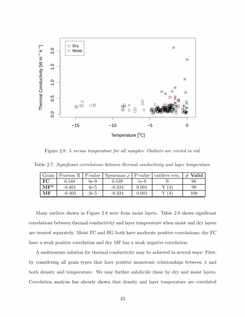
−15 −10 −5 0
0.0
0.5
1.0
1.5
2.0
Temperature [oC]
The
rmal
Con
duct
ivity
[W m
−1 k
−1 ] Dry
Moist
Figure 2.8: λ versus temperature for all samples. Outliers are circled in red.
Table 2.7: Significant correlations between thermal conductivity and layer temperature.
Grain Pearson R P-value Spearman ρ P-value outliers rem. # ValidFC 0.548 8e-9 0.539 1e-8 N 96MF* -0.401 4e-5 -0.324 0.001 Y (4) 99MF -0.403 2e-5 -0.324 0.001 Y (4) 108
Many outliers shown in Figure 2.8 were from moist layers. Table 2.8 shows significant
correlations between thermal conductivity and layer temperature when moist and dry layers
are treated separately. Moist FC and RG both have moderate positive correlations; dry FC
have a weak positive correlation and dry MF has a weak negative correlation.
A multivariate solution for thermal conductivity may be achieved in several ways: First,
by considering all grain types that have positive monotonic relationships between λ and
both density and temperature. We may further subdivide these by dry and moist layers.
Correlation analysis has already shown that density and layer temperature are correlated
43

−15 −10 −5 0
0.0
0.1
0.2
0.3
0.4
Temperature [oC]
The
rmal
Con
duct
ivity
[W m
−1 k
−1 ] Dry
Moist
Figure 2.9: λ versus temperature for melt-freeze (MF) forms.
with thermal conductivity, at least for some grain types. Based on the scatter plots in this
study as well as the results of Sturm et al. (1997) linear or quadratic models would be
expected to provide the best fit.
Potential models were investigated using the linear model fitting ‘lm’ function in the
statistical software suite R (R Core Team, 2013). A backwards stepwise regression was
performed against λ to see whether a multivariate model actually offers a better solution than
Table 2.8: Correlations between thermal conductivity and layer temperature by treating dryand moist layers separately.
Grain Type Pearson R P-value Spearman ρ P-value outliers rem. # ValidFC moist 0.71 5e-5 0.662 2.33e-4 N 26FC dry 0.596 5e-8 0.458 6.63e-5 N 70RG moist 0.768 0.016 0.735 0.024 N 9MF dry -0.490 5e-5 -0.399 0.001 Y (2) 62
44
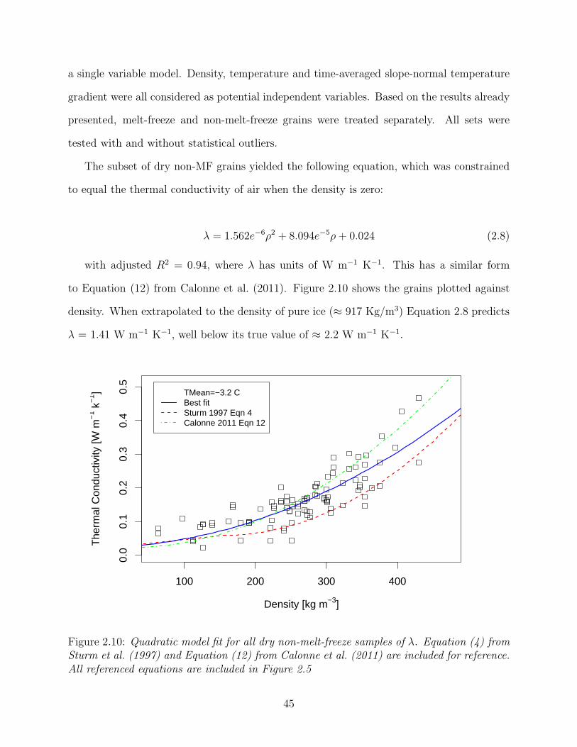
a single variable model. Density, temperature and time-averaged slope-normal temperature
gradient were all considered as potential independent variables. Based on the results already
presented, melt-freeze and non-melt-freeze grains were treated separately. All sets were
tested with and without statistical outliers.
The subset of dry non-MF grains yielded the following equation, which was constrained
to equal the thermal conductivity of air when the density is zero:
λ = 1.562e−6ρ2 + 8.094e−5ρ+ 0.024 (2.8)
with adjusted R2 = 0.94, where λ has units of W m−1 K−1. This has a similar form
to Equation (12) from Calonne et al. (2011). Figure 2.10 shows the grains plotted against
density. When extrapolated to the density of pure ice (≈ 917 Kg/m3) Equation 2.8 predicts
λ = 1.41 W m−1 K−1, well below its true value of ≈ 2.2 W m−1 K−1.
100 200 300 400
0.0
0.1
0.2
0.3
0.4
0.5
Density [kg m−3]
The
rmal
Con
duct
ivity
[W m
−1 k
−1 ] TMean=−3.2 C
Best fitSturm 1997 Eqn 4Calonne 2011 Eqn 12
Figure 2.10: Quadratic model fit for all dry non-melt-freeze samples of λ. Equation (4) fromSturm et al. (1997) and Equation (12) from Calonne et al. (2011) are included for reference.All referenced equations are included in Figure 2.5
45

Although Equation 2.8 fits the measured data relatively well, it is likely less accurate for
snow with very low or very high densities. When compared to the best-fit equation from
Sturm et al. (1997) the disparity between their data set and ours becomes evident. There
are several possible reasons but the most likely is that our mean temperature was almost 10
◦C warmer than the majority of their samples. Unfortunately temperature did not emerge
as a significant variable for this subset of data. For the subset of moist non-melt-freeze
grains layer temperature did emerge as a significant ( p ≤ 0.05) predictor as part of a linear
model of the form λ = a+ bρ + cT, but extrapolations beyond the relatively narrow range
of temperatures yielded unrealistic values of λ. It should be noted that although moist
grains should, by definition, exist only at 0.0 ◦C layers were sometimes classified as such
even though the measured temperature was colder. Possible reasons for this discrepancy
include strong insolation on many of the study days and the relatively crude nature of the
‘glove test’ (CAA, 2007). Temperature was also a significant predictor for the subset of dry
MF grains while density was not. The equation,
λ = 0.140− 0.010T (2.9)
gives an adjusted R2 = 0.24. The independence of thermal conductivity from density
in MF layers has already been discussed; however, the decreasing values with warmer layer
temperatures does not intuitively make sense. Although this result cannot be dismissed
outright it seems more likely that it is due to the character of the cold lab crusts, which were
from a single site and make up all measurements below -10 ◦C.
Subsection 2.6.2 Summary
This section probed for statistically significant relationships between physical parameters
of the snowpack and measured thermal conductivity. Parameters were restricted to those
commonly measured in the field, that is density, layer temperature, temperature gradient,
moisture and grain type. As with previous studies, density was typically the single best
46

predictor of thermal conductivity for all grain types except for melt-freeze crusts. When
compared with the empirical equations of Sturm et al. (1997) our data show similar trends
but our values of thermal conductivity were typically higher. There is very likely a tem-
perature dependence as the majority of our measurements were made at warmer snowpack
temperatures but layer temperature did not emerge as a significant predictor variable. These
findings are similar to those published by Sturm et al. (1997) with the possible exception
that for our samples density was a good predictor for thermal conductivity in samples that
had undergone kinetic (temperature gradient) metamorphism. This difference is likely one
of semantics as their data included samples of depth hoar and highly faceted grains, while
our ‘facets’ were typically transitional forms, barely differentiable from rounded grains.
Although field methods do not permit the level of precision offered by a model there are
some worthwhile avenues to explore in future studies: 1) Dry and moist layers should be
treated separately during analysis due to the increased presence of free water. In reality
the change in actual water content is gradual but this distinction appears to be sufficient
if precise measurements are not possible; 2) Grain type may be broadly treated as ‘MF’ or
‘non-MF’. Our data set did not include depth hoar but based on work by Sturm and Johnson
(1991) they should also be treated as a separate grain type; 3) Empirical equations based
on density alone do illuminate trends but they are not sufficient on their own as predictive
equations. Other parameters, likely temperature, need to be incorporated but our data did
not include enough measurements over a wide enough range to accomplish this.
2.6.3 Thermal conductivity by site
The main goals of measuring crust thermal conductivity were to document rates of change
and to identify significant correlations with other measured parameters. This knowledge is
primarily useful for use in physical models such as SNOWPACK (Bartelt and Lehning, 2002)
but also in mesoscale and climate weather models (e.g. Cook et al., 2008) that depend on
parameterizations to model physical characteristics of ground cover including snow. This
47

section examines temporal changes in individual crusts.
Detailed information regarding the study sites and narratives of crust formation and
evolution are included in Appendix A and all measurements are given in Appendix C. Mea-
surement intervals for each crust are outlined in Table 2.2. Measurements were taken above,
below and within the crust each field site except for SR09. Measurements of vertical thermal
conductivity were taken at some field sites and for all cold lab experiments. Temperature
and vertical temperature gradient were monitored with thermistors at some field sites and
throughout all but one cold lab experiment. Temperature profiles were also measured man-
ually at field sites during each visit as part of a standard test profile. It is worth reiterating
that the convention used througout this paper is that a negative temperature gradient means
colder temperatures closer to the snow surface.
Study sites FI0109 and FI0308 were both located at the Mount Fidelity study plot ad-
jacent to the weather station. More information on this and other study is included in
Appendix A and in Figure A.4. FI0109 formed as a thin ice lens in early January 2010.
Thermal conductivity was tracked within the crust when possible as well as in the layers
above and below throughout the remainder of the season. The layers at this site were buried
relatively quickly and thus remained viable for sampling throughout the remainder of the
season, through April 14. Figure 2.11 shows the evolution over time of thermal conductivity
in the layer immediately above the crust and Figure 2.12 shows the layer below. The error
bars represent the instrument error published by Hukseflux, the manufacturer of the TP02
instrument (Hukseflux, 2003). Grains in both layers progressed over time from precipitation
particles (PP) to mixed forms (either RGxf or FCxr).
Thermal conductivity increases over time in both layers, with increased variability evident
by early March. The thermal conductivity was positively correlated with density in both
layers which is to be expected given the relationship already reported in the previous section.
Both layers also had a moderately strong positive relationship between thermal conductivity
48

Jan
10
Jan
10
Jan
18
Jan
18
Jan
25
Jan
25
Jan
25
Feb
02
Feb
02
Feb
02
Feb
08
Feb
08
Feb
17
Feb
17
Feb
28
Feb
28
Mar
09
Mar
09
Mar
15
Mar
15
Mar
22
Mar
22
Mar
28
Apr 0
7
Apr 1
4
0
0.2
0.4
0.6T
herm
al C
ondu
ctiv
ity [W
/(m
K)] Moist samples
Figure 2.11: Time series of thermal conductivity measurements in the layer above the FI0109crust. Error bars denote range of possible values based on the thermal conductivity probemanufacturer’s stated accuracy. Two measurements were attempted during each site visitbut some were invalid.
and layer temperature, as shown in Table 2.9.
Removing the moist layers from the correlation calculation did not affect the correlations
between λ and layer temperature in either case, which runs counter to what was found in the
previous section and may hint that this effect was more a function of specific layers in the
dataset than it was a function of free water in each layer. Although calibrated thermistors
and thermocouples were deployed at this site, they were inserted immediately above and
Table 2.9: Pearson correlations between λ, density (ρ) and layer temperature (T) for layersabove and below the FI0109 crust. All correlations are significant to p ≤ 0.01.
Layer ρ ρ range [kg m−3] T T range (◦C) Grains # ValidAbove 0.83 97-397 0.78 -4.7,-1.6 PP,FCxr/RGxf 25Below 0.79 112-430 0.80 -4.8,-1.1 PP,FCxr/RGxf 27
49

Jan
10
Jan
10
Jan
12
Jan
12
Jan
18
Jan
18
Jan
25
Jan
25
Feb
02
Feb
02
Feb
02
Feb
02
Feb
08
Feb
08
Feb
17
Feb
17
Feb
28
Mar
09
Mar
09
Mar
15
Mar
15
Mar
22
Mar
28
Mar
28
Apr 0
7
Apr 1
4
Apr 1
4
0
0.2
0.4
0.6T
herm
al C
ondu
ctiv
ity [W
/(m
K)] Moist samples
Figure 2.12: Time series of thermal conductivity measurements in the layer below the FI0109crust at Mt Fidelity study plot.
below the crust so no analysis could be performed on rates of change of λ with respect to
the vertical temperature gradient. Test profiles did note several very modest temperature
gradients, on the order of 0.1 ◦C 10 cm−1 both above and below the crust.
Crust FI0308 formed during a period of warm weather and intense insolation in early
March 2010. Unlike FI0109 it was thick enough to sample with the TP02 probe, however
there were no identifiable temporal trends. Figures 2.13 and 2.14 show the time series for
the layers above and below the FI0308 crust. As was the case with the layers above and
below FI0109 the strongest correlations are between thermal conductivity and density. The
correlation between layer temperature and λ was only statistically significant for the layer
below the crust, and was improved when the moist samples were removed from the data set.
This result is not included in Table 2.10 due to the small sample size.
The final natural crust presented here is RP0112. It formed in the study plot at Rogers
50

Mar
15
Mar
15
Mar
22
Mar
22
Mar
28
Mar
28
Apr 0
7
Apr 1
4
Apr 1
4
0
0.2
0.4
0.6T
herm
al C
ondu
ctiv
ity [W
/(m
K)] Moist samples
Figure 2.13: Time series of thermal conductivity measurements in the layer above the FI0308crust.
Table 2.10: Pearson correlations between λ, density (ρ) and layer temperature (T) for layersabove and below the FI0308 crust. All correlations are significant to p ≤ 0.05.
Layer ρ ρ range [kg m−3] T T range (◦C) Grains # ValidAbove 0.87 166-310 ∼ -3.7,-1.8 DF,MF,RG 9Below 0.98 228-332 0.78 -3.7,-1.8 FCxr,RGxf 8
Pass at the same time as BV0112 but was not subject to the continuous insolation and
warm temperatures as the latter was due to its slightly higher elevation and shaded location.
Time series plots of the layers above and below are shown in Figures 2.15 and 2.16. While
both layers do appear to undergo a moderate increase in thermal conductivity, much of the
week-to-week variability is within the bounds of the measurement error of the TP02. The
layer above the crust has a moderately strong positive correlation between λ and density (R
= 0.79, p ≤ 0.01) but that is the only correlation. The crust itself was noted to have many
51

Mar
15
Mar
15
Mar
22
Mar
22
Mar
28
Apr 0
7
Apr 1
4
Apr 1
4
0
0.2
0.4
0.6T
herm
al C
ondu
ctiv
ity [W
/(m
K)] Moist samples
Figure 2.14: Time series of thermal conductivity measurements in the layer below the FI0308crust.
icy inclusions and showed no visually or statistically identifiable trends or correlations.
The first attempts at cold lab experiments used sifted snow and manual wetting to create
a uniform crust. These attempts were largely unsuccessful and usually resulted in percolation
channels and inhomogeneous ice layers within the sifted snow. Later attempts at compacting
the snow before wetting were also unsuccessful in creating a homogeneous crust. As a result
natural crusts were harvested into an insulated box (shown in Figure 2.17) from a flat area
near the residences at Rogers Pass and brought into the lab, where thermistors mounted on
wood blocks 10 cm apart were inserted into the sample. A strong temperature gradient was
induced by harvesting the crusts during the daytime and placing the uncovered box into the
cold lab. The insulated base and size ensured that lower portions of the sample remained
warm, at least initially, while upper portions of the crust quickly cooled. The size of the
box limited the total number samples to around six and the measurement intervals were
lengthened for each experiment to try and determine the time scale of changes in thermal
52
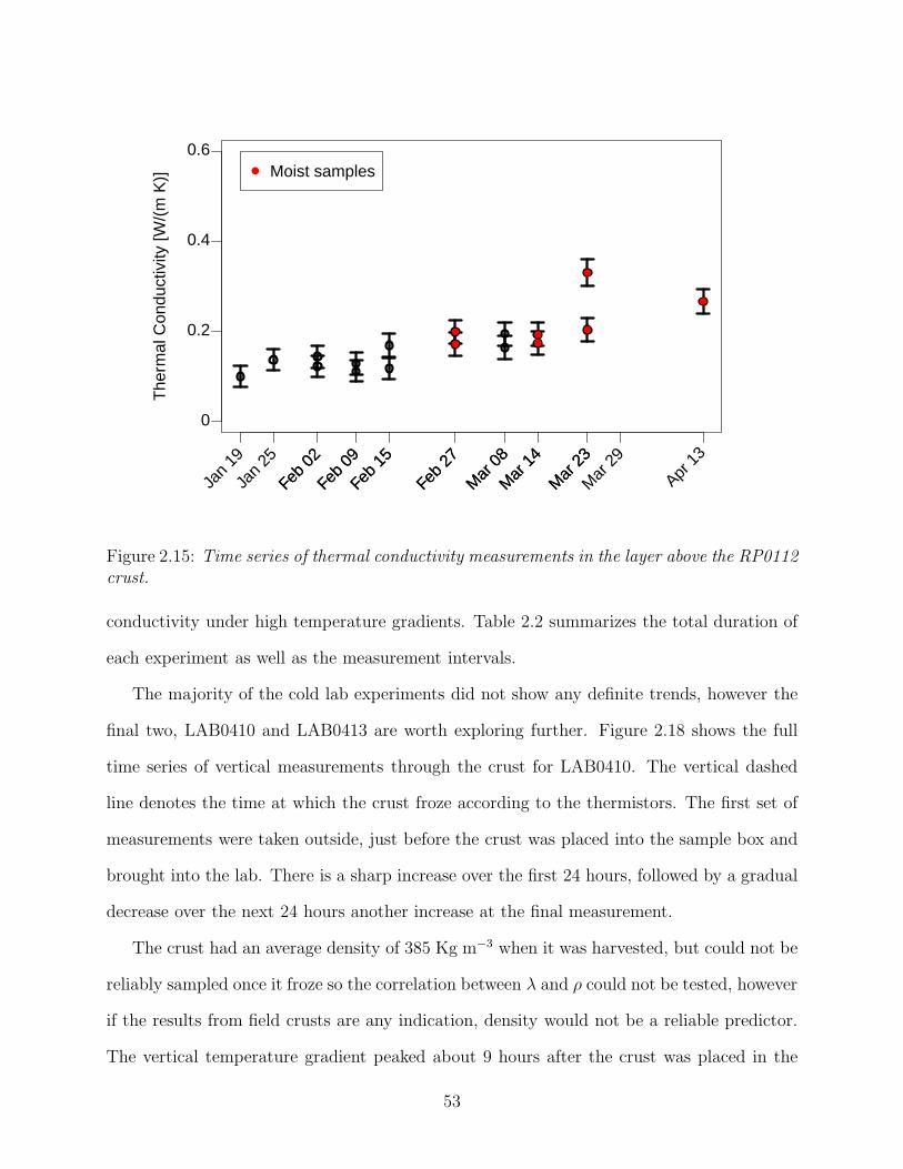
Jan
19
Jan
25
Feb
02
Feb
02
Feb
09
Feb
09
Feb
15
Feb
15
Feb
27
Feb
27
Mar
08
Mar
08
Mar
14
Mar
14
Mar
23
Mar
23
Mar
29
Apr 1
3
0
0.2
0.4
0.6T
herm
al C
ondu
ctiv
ity [W
/(m
K)] Moist samples
Figure 2.15: Time series of thermal conductivity measurements in the layer above the RP0112crust.
conductivity under high temperature gradients. Table 2.2 summarizes the total duration of
each experiment as well as the measurement intervals.
The majority of the cold lab experiments did not show any definite trends, however the
final two, LAB0410 and LAB0413 are worth exploring further. Figure 2.18 shows the full
time series of vertical measurements through the crust for LAB0410. The vertical dashed
line denotes the time at which the crust froze according to the thermistors. The first set of
measurements were taken outside, just before the crust was placed into the sample box and
brought into the lab. There is a sharp increase over the first 24 hours, followed by a gradual
decrease over the next 24 hours another increase at the final measurement.
The crust had an average density of 385 Kg m−3 when it was harvested, but could not be
reliably sampled once it froze so the correlation between λ and ρ could not be tested, however
if the results from field crusts are any indication, density would not be a reliable predictor.
The vertical temperature gradient peaked about 9 hours after the crust was placed in the
53

Jan
19
Jan
25
Feb
02
Feb
02
Feb
09
Feb
09
Feb
15
Feb
15
Feb
27
Feb
27
Mar
08
Mar
08
Mar
08
Mar
08
Mar
14
Mar
14
Mar
23
Mar
23
0
0.2
0.4
0.6T
herm
al C
ondu
ctiv
ity [W
/(m
K)] Moist samples
Figure 2.16: Time series of thermal conductivity measurements in the layer below the RP0112crust.
cold lab, just about the time that it became fully frozen. The crust temperature ranged
from -0.1 ◦C at the start of the experiment to -15.1 ◦C at the end, while the average vertical
temperature gradient between observations varied from -2.96 ◦C 10 cm−1 to -0.06 ◦C 10 cm−1
at the conclusion of the experiment.
In this crust there were likely two competing processes affecting the thermal conductivity:
As the moist layer froze new bonds were formed enabling more efficient transport of heat
through the grain matrix. At the same time, a strong vertical temperature gradient would
favour formation of vertically oriented bonds, but would also result in at least some faceting,
which would increase the tortuosity and decrease the number of thermal pathways. Other
studies have observed the preferential formation of vertical bonds when a sample of natural
snow was subjected to continuous strong vertical temperature gradients in the lab (Greene,
2007) and the same mechanism has been hypothesized for natural depth hoar (Sturm and
Johnson, 1992).
54

Figure 2.17: Schematic of the insulated box used for cold lab experiments. The front andsides are insulated with foam while the top is left uncovered.
There were no significant ( p ≤ 0.05 ) correlations between the rate of change of λ and
average temperature, temperature gradient or time. It is possible that the relatively small
sample size precludes the identification of any statistically significant correlations, or that a
combination of factors is responsible for the observed changes.
The LAB0413 time-series is shown in 2.19. Sampling was done daily over a period of
5 days at intervals of approximately 24 hours each. As was the case with other cold lab
experiments, a density sample was only obtained during the initial sampling before the crust
was brought into the cold lab. This 40 cm thick sample averaged 385 Kg m−3 before it
was placed into the insulated box. No settlement was observed during the course of the
experiment. The trend in thermal conductivity closely mirrors that seen in LAB0410, with
an initial increase over the first 48 hours. Unlike LAB0410 a weak trend of decreasing thermal
conductivity continues through the end of the experiment.
Figure 2.20 shows the corresponding time series of average layer temperature and tem-
perature gradient for the crust. Initially the upper portions of the crust are warmer but by
12 hours into the experiment the gradient reverses and remains equal or greater to 1 ◦C 10
cm−1 until approximately the third day. Table 2.11 shows the correlations between changes
55

04/1
0 19
:15
04/1
0 19
:15
04/1
1 09
:30
04/1
1 09
:30
04/1
1 21
:00
04/1
1 21
:00
04/1
2 09
:40
04/1
2 21
:05
04/1
2 21
:05
04/1
3 09
:35
04/1
3 09
:35
0
0.2
0.4
0.6T
herm
al C
ondu
ctiv
ity [W
/(m
K)] Vertical meas.
Moist samples
Figure 2.18: Time series of thermal conductivity measurements for LAB0410. The verticaldashed line denotes the time at which the crust froze.
over time in λ and both layer temperature and temperature gradient for this crust. The rate
of change of thermal conductivity between measurements is strongly correlated in this case
with the average temperature between measurements. Taken together with the correlation
with the average temperature gradient a plausible physical explanation is that the initial
sharp increase in thermal conductivity is due to bonds freezing, followed by the preferential
formation of vertical bonds as the temperature gradient reaches a maximum. The link with
the observed decrease in thermal conductivity over the final seventy-two hours is less clear,
but may be related to continued faceting in the crust. This interpretation could be tested
by conducting a similar experiment where the crust is cooled and then re-warmed over a
similar time period.
Figure 2.21 shows a time series of thermal IR images taken immediately after a new
crust face was exposed at each observation time. The image in the upper left was taken
56

Apr 1
3
Apr 1
4
Apr 1
5
Apr 1
5
Apr 1
6
Apr 1
6
Apr 1
7
Apr 1
7
Apr 1
8
Apr 1
8
0
0.2
0.4
0.6T
herm
al C
ondu
ctiv
ity [W
/(m
K)] Vertical meas.
Moist samples
Figure 2.19: Time series of thermal conductivity measurements for LAB0413.
just after the crust was brought into the cold lab. The area of uniform temperature has
just been exposed and the strips to each side had already had the chance to cool for several
minutes. The overburden layer has cooled substantially by the next observation and the
effects of imperfect insulation from the walls of the box are evident as only a small area of
the lower crust remains near freezing while the sides have frozen. By the second observation
at 50 hours this effect is still evident, though less pronounced and by 73 hours the crust’s
Table 2.11: Pearson correlations between rates of change of λ, average layer temperature (col-umn 6) and average temperature gradient (column 7) for the LAB0413 crust. All correlationsare significant to p ≤ 0.05.
∆λ ∆λ
λ T TG # Valid Tavg between meas. TGavgCrust range range range meas. λ ∼Tavg λ ∼TGavgLAB0413 0.08-0.41 -1.5,-8.6 -0.1,-2.5 10 0.86 -0.68
57

−10
−8
−6
−4
−2
0
Tem
pera
ture
[o C]
TTG
04/1
3 19
:00
04/1
4 07
:00
04/1
4 19
:00
04/1
5 07
:00
04/1
5 19
:00
04/1
6 07
:00
04/1
6 19
:00
04/1
7 07
:00
04/1
7 19
:00
04/1
8 07
:00
04/1
8 19
:00
−2.0
−1.8
−1.6
−1.4
−1.2
−1.0
−0.8
−0.6
−0.4
−0.2
0.0
Tem
pera
ture
Gra
dien
t [o C
10
cm−
1 ]
Figure 2.20: Time series of average layer temperature and vertical temperature gradient forthe crust in LAB0413.
temperature is mostly uniform.
Figure 2.22 shows the crust at 99 hours with a reduced temperature scale. Relatively
small variations in crust temperature can still be seen, and would not likely be identified using
conventional thermometers or thermistors. This series of images shows the complexities of
thermal pathways even in a relatively simple 2-dimensional environment. It is important to
note that some recent research (Schirmer and Jamieson, 2014) indicates that a combination
of inhomogeneous snow surfaces and sharp contrasts between snow and air temperature may
result in false temperature gradients in thermal IR photography and video. The use of
thermal IR methods for qualitative or illustrative purposes as it is done here is likely safe.
As with LAB0410 the change in thermal conductivity was affected by the competing
processes of freezing during the initial part of the experiment and faceting as a sharp vertical
58

temperature gradient developed. This is evident both in the time series of thermal infrared
images as well as the moderate correlation between rates of change of λ and the average
temperature gradient.
Figure 2.21: Montage of thermal IR images of crust LAB0413 as it was cut back and exposedfor each observation. The ruler is visible in most images as a vertical discontinuity.
Samples from the South Run (SR) and Beaver Valley (BV) sites did not show any tem-
poral trends or correlation with other measured physical parameters such as density, layer
temperature or average vertical temperature gradient. Snow at these sites was subject to
both strong insolation (South Run) and persistent warm air temperatures due to low eleva-
tion (Beaver Valley) and layers remained moist for extended periods at both sites.
Subsection 2.6.3 Summary
This section presented a summary of time series measurements of natural layers in the
field and in a cold lab. Most crusts did not yield any statistically significant correlations with
regards to thermal conductivity or rates of change of thermal conductivity. The exception
was the final cold lab crust, LAB0413 where the rate of change of λ was correlated with both
the layer temperature and the average vertical temperature gradient. A number of non-MF
layers did have significant correlations between λ and density. Taken together with results
59

Figure 2.22: Thermal IR image at 99 hours, scaled to show small variations in temperature.
from the previous section, the evolution of thermal conductivity can be predicted, with some
error, without precise knowledge of the grain form as long as it is not highly faceted.
The data set had a number of shortcomings, some due to the experimental design and
others due to the relatively warm winter of 2009-10: 1) Crust samples in the cold lab exper-
iment were too small and often too brittle once frozen to accurately measure density, even if
it likely does not correlate well with thermal conductivity; 2) With the exception of cold lab
crusts, the small range of temperatures in all tracked layers made correction for temperature
virtually impossible; 3) Temperature and temperature gradient were not tracked in layers
above and below natural crusts, negating an opportunity to link them to rates of change of
λ; 4) The thermal IR camera was only available for short periods and it is likely that the
presence of small temperature gradients was missed, especially at crust boundaries.
Given these results, future experiments should focus on measuring thermal conductivity
under measurable and controllable conditions in a cold lab. The most interesting results were
from LAB0413, where the thermal conductivity peaked just after the entire crust froze, then
gradually diminished through the end of the experiment. These observations are consistent
with results published by Kaempfer et al. (2005) as well as the theoretical pathways proposed
60

by Kaempfer and Schneebeli (2007), Kaempfer et al. (2009) and Shertzter et al. (2010).
Structural changes identified by Near IR photography are covered in Chapter 3.
2.6.4 Spatial variability of thermal conductivity
A significant assumption when tracking changes over time is that a given layer began with
uniform physical properties and all changes occurred uniformly within a study plot on the
order of several metres square . As many studies (e.g. Campbell and Jamieson, 2007; Landry,
2002; Schweizer et al., 2008; Buhler and Jamieson, 2012) have found, this can be a problem-
atic assumption when applied to snowpack stability and thus presumably to the structure of
a given layer. This may be a reasonable assumption if the site is relatively small and if the
meteorological conditions contributing to the layer formation are known. This can become
complicated for melt-freeze crusts due to how they are formed: A rain crust will almost cer-
tainly have percolation channels and icy inclusions while crusts formed due to above-freezing
temperatures and/or direct insolation may be more uniform depending on the duration and
intensity of the heating.
Since measurements of thermal conductivity in buried layers are necessarily destructive
it is not possible to measure the initial spatial variability for the field sites described in
this chapter. This uncertainty is offset somewhat by selecting sheltered sites and by taking
multiple measurements of thermal conductivity during each site visit. It is also possible to
test these assumptions to a certain extent by taking spatial measurements across a site that
should be uniform.
Figure 2.23 shows a planar south-facing slope on the ”South Run“ area of Mt. Fidelity
on February 5, 2010. In late January a melt-freeze crust formed here due to solar radiation
and was buried January 31. Thermal conductivity was measured at 2 m intervals across an
area 20 m2. The sample area was planar with sparse mature timber adjacent on either side.
Due to the low angle of the sun in January as well as blocking by surrounding topography,
the entire sample area received approximately uniform insolation during the period of crust
61

Figure 2.23: South-facing site used to evaluate spatial variability.
formation. The crust was of uniform visual appearance and thickness across all sample sites.
Figure 2.24 shows the measured thermal conductivity (in red) and the layer temperature
(in black) at each sample location. The right transect has a slightly lower mean thermal
conductivity, possibly due to shading from the single tree visible in Figure 2.23. There are no
clear trends in the upslope direction, nor is there a relationship between layer temperature
and thermal conductivity in this sample. Near-infrared photographs taken at each sample
site showed qualitatively similar profiles of specific surface area and are discussed further in
Chapter 3.
The results in this section illustrate that great care must be taken in selecting study
sites for tracking changes in thermal conductivity. It is likely that the conditions under
which a layer is formed and before it is buried are important in determining its initial spatial
variability. This does not imply that, for example, rain crusts cannot be tracked over time,
but that during analysis care must be taken to separate temporal trends from spatial trends.
62

2.5 2.0 1.5 1.0 0.5 0.0 −0.5
02
46
810
Cross−slope distance [m]
Ups
lope
dis
tanc
e [m
]
0.081
0.087
0.115
0.093
0.084
0.114
0.111
0.092
0.113
0.085
0.165
−0.9
−1.4
−2
−2.6
−1.4
−2.7
−1.5
−1.4
−1.5
−2
−2.4
Figure 2.24: Thermal conductivity measurements on a planar south-facing slope. Numbersin red are thermal conductivity and numbers in black are layer temperature, both recordedconcurrently.
63

Evidence for the former may be supported by measurements of density, temperature and
temperature gradient or by visual observations of structure. Potential study sites should
also be carefully evaluated for any factors such as vegetation, slope, aspect or exposure to
wind that may increase the spatial variability.
2.7 Chapter Summary
Thermal conductivity was measured over time in five natural crusts and five crusts in the
cold lab. For natural crusts the thermal conductivity of layers above and below the crust
was also monitored. The Hukseflux TP02 thermal conductivity probe was found to be an
effective instrument for both field-based and lab-based studies. A number of difficulties were
encountered, most having to do with the warm temperatures and low snowfall during the
winter of 2009-10 in southwestern British Columbia.
Thermal conductivity measurements were grouped according to grain type and compared
with previous studies including the data published in Sturm et al. (1997). Distributions for
each grain type were tested for normality using the Shapiro-Wilk Normality test. It should
be noted that the Shapiro-Wilk implementation in R uses an extension (Royston, 1995) of
the original test which is valid for samples up to n = 5000. The null hypothesis of normality
for all grain types was rejected based on the presence of a small number of outliers in each
data set. This was especially prevalent in layers that had been classified as moist. When
outliers were removed, then mean thermal conductivity of non-MF grains were similar to
those published by Sturm et al. (1997).
The subset of melt-freeze (MF) grains was especially varied with the highest and lowest
measured values approaching those of pure ice and air respectively. Two new subsets were
created; pure MF (MF*) and MF containing aggregates of faceted forms (MFFC). The mean
thermal conductivity of the former was similar to the mean for ‘melt grain clusters’ reported
by Sturm et al. (1997).
64
Correlations were computed between λ and easily measurable physical parameters such
as layer temperature and density. The influence of outliers and of layer moisture was also
checked. The strongest correlations between density and λ were found for FC and RG
grain types. The correlation between ρ and λ runs counter to conclusions published by
Sturm et al. (1997) and illustrates a difficulty in using grain type classifications; it is very
likely that the FC in the present study were less faceted, and had settled and bonded to
a greater degree than those measured by Sturm. Though not directly applicable to MF
grain types, the observations of Calonne et al. (2011) and Greene (2007) that faceting is not
necessarily accompanied by changes in density may be relevant, in that the MF classification
encompasses a wide variety of structures from poorly-bonded clusters to uniform well-bonded
layers.
Empirical equations from Sturm et al. (1997) matched the general trend of increasing λ
with increasing density but actual predicted values of λ were consistently lower than mea-
sured values from the present study. Attempts were made to formulate a new empirical
equation but layer temperature did not emerge as a significant predictor. A polynomial
equation with a similar form to Sturm’s was produced for the set of all dry non-MF forms.
Like Sturm’s it is likely of limited value outside of the range of temperature from the dataset
from which it was derived. If the data from Sturm’s study, which were measured at much
colder temperatures, were combined with those of the present study it is possible that layer
temperature could be incorporated as a statistically significant predictor in a more general-
ized empirical equation.
Time series of individual layers were examined for trends in thermal conductivity and
correlation with layer temperature, density and temperature gradient. In this case several
layers showed good correlations between λ and both density and layer temperature suggesting
that the characteristics of the individual layer are as important as the grain type for non-MF
forms.
65
Two cold lab crusts, LAB0410 and LAB0413 showed similar trends in thermal conduc-
tivity. Both showed increases in λ until some time after the crust was frozen, then a slow
decrease. A potential explanation for these observations is the formation of oriented bonds as
the layer slowly freezes thus increasing λ, followed by faceting due to the unequal cooling of
the crust from the top down. A series of thermal infrared images taken during the LAB0413
experiment confirms that sharp vertical temperature gradients were present well after the
crust was frozen.
The results from this chapter offer several avenues for future research: 1) The results from
the present study should be combined with those of Sturm to examine more thoroughly the
effects of layer temperature on thermal conductivity. Their data were gathered at much
colder temperatures while ours, with the exception of cold lab crusts, were often just below
freezing. Should that attempt be successful the role of moisture may also become more
evident; 2) Further cold lab studies should be conducted with melt-freeze crusts. The re-
sults from LAB0410 and LAB0413 match hypotheses proposed by Kaempfer and Schneebeli
(2007) and Kaempfer et al. (2009) regarding increased tortuosity and changes in thermal
pathways under strong temperature gradients. These studies should include the sampling of
temperature as well as both vertical and horizontal measurements of thermal conductivity.
Temperature measurements should be supplemented with thermal IR photography as the
detail offered by embedded thermistors or thermocouples does not offer sufficient spatial
resolution to identify small and transient temperature gradients.
66

Chapter 3
Near Infrared Photography
continuous process rather than a set of discrete steps it is easy to miss gradual transitions.
In recent years the use of optical methods to quantify snowpack morphology, rather than size
and shape, has seen increased use. Snow morphology influences the spectral albedo of snow
(e.g. Wiscombe and Warren, 1980; Warren and Wiscombe, 1981) and has important impli-
cations in many fields of study outside of avalanche research, including remote sensing (e.g.
Toure et al., 2008), climate modeling (e.g. Flanner and Zender, 2006) and snow chemistry
(Douglas et al., 2008).
This chapter introduces the theory behind NIR and SSA and summarizes the results
of studies by other authors. The equipment, field techniques and methods of analysis are
summarized and results from this study from the winters of 2008-09 and 2009-10 are pre-
sented. It is important to note that the NIR portion of the solar spectrum is defined here as
wavelengths between 700 nm and 2000 nm, and the meaning of the term varies somewhat
across disciplines.
3.1 Specific surface area (SSA) theory and past studies using optical meth-
ods
specific surface area (SSA) is defined as the ratio of surface area to volume of a given sample of
snow or ice crystals, with units of mm−1. In some cases it is reported as the ratio of the surface
area to volume times the density of ice and has units of m2 kg−1. It generally decreases over
time (Legagneux et al., 2003), and at accelerated rates at warmer temperatures (Taillandier
et al., 2007) as new snow transitions from dendritic to rounded forms, though Domine et al.
(2009) record three instances where it increased. Various empirical (e.g. Domine et al., 2007)
67
and prognostic (e.g. Jacobi et al., 2010) equations based on grain type or density have been
proposed but there has been little practical validation for melt-freeze layers.
Prior to the late 1990s the only option for measurement of SSA was to use stereological
methods. This required that samples either be cultivated in, or transported to a cold lab
as well as access to specialized equipment. Aside from the difficulties in preserving natural
snow samples, stereological techniques are time-consuming and may only measure small
samples. In the past 15 years new imaging techniques have emerged, allowing sampling to
be done relatively quickly and, as importantly, directly at field sites. Haddon et al. (1998)
first published an experimental algorithm for the analysis of near infrared (NIR) images of
snow profiles. Matzl and Schneebeli (2006) modified a digital camera with an 830 nm filter
and correlated in-situ NIR photographs with SSA measured using stereological techniques.
Calibrated NIR photographs could be mapped to measured SSA using an empirical equation
with a correlation of 90%. This technique was found to be valid for layers as thin as 1
mm although results may be susceptible skewed by light leaking from adjacent layers (Matzl
and Schneebeli, 2010). The importance of this light leakage when observing buried layers is
debatable as radiation at NIR wavelengths does not penetrate far into the snowpack, with
estimates ranging from 3.5 cm (Gallet et al., 2009) to 1-5 cm (Kokhanovsky and Rozanov,
2012), depending on the precise wavelength and grain geometry. The NIR spectrum above
900 nm has the additional property of weak sensitivity to impurities within the snow sample
(Grenfell et al., 1981).
Toure et al. (2008) used techniques similar to those of Matzl and Schneebeli (2006) to
derive the correlation length from the calculated SSA, while Tape et al. (2010) used similar
equipment and techniques to quantify lateral variability in a sub-arctic snowpack, but did
not calculate the SSA. Langlois et al. (2010) used a modified digital camera similar to that
used by Matzl and Schneebeli (2006) but used a 750 nm filter and added 840 nm and 1000
nm filters in successive steps. The authors found that the geometric diameter, defined as
68

the average of the major and minor axis diameters, was weakly correlated with NIR, and
that a stronger correlation might have been possible with an instrument sensitive to longer
wavelengths. The reclassification of grain types into broad classes of ‘large’, ‘medium’ and
‘small’ spheres, and by assuming a shape factor for each (Kokhanovsky and Zege, 2004), it
was also possible to retrieve the optical grain diameter from NIR photographs.
Gallet et al. (2009), and later Morin et al. (2010) used an active laser diode-equipped
instrument known at DUFISSS to measure the reflectance of snow, then converted it to
reflectance and SSA. The advantage of this instrument is that it emits at a single wavelength
(1310 nm) and allow results to be integrated into radiative transfer models with greater ease.
Despite numerous field and modeling studies, there has been little research into SSA
of melt-freeze crusts. These layers present particular difficulties as traditional assumptions
regarding metamorphism are not always applicable: Although several studies have examined
the formation of weak layers at the boundaries of crusts or buried wet layers under relatively
high temperature gradients (e.g. Greene, 2007; Jamieson and Fierz, 2004), a number of
experienced practitioners have also reported the development of facets and laminations in
buried crusts even when the temperature gradient as measured by traditional means would
imply such such weakening should not take place (John Hetherington, pers. comm. 2009 ).
The advent of models such as CROCUS (Brun et al., 1992) and SNOWPACK (Bartelt and
Lehning, 2002; Lehning et al., 2002a,b) promise to mitigate some of these challenges; however
many processes at the microstructural level are not well-understood and consequently not
always well-modeled. Jacobi et al. (2010) tested both empirical and prognostic equations for
SSA in the CROCUS model and found that both tended to overestimate the values. Morin
et al. (2010) performed a field validation of SSA in the same model and concluded that
although the model performed well, there was ample room for improvement.
NIR photography was used in the present study with the goal of tracking changes over
time of SSA in melt-freeze crusts, both in the field and in the cold lab where conditions may
69
be better controlled. The equipment and techniques introduced by Matzl and Schneebeli
(2006) were chosen for their relatively low cost and ease of use in the field environment.
3.2 Equipment and Field Methods
When tracking temporal changes in a type of snow known to be spatially variable (e.g.
Schweizer et al., 2008) it is critical to gather as much information as possible about the
initial structure. By careful selection of study sites and by monitoring the meteorological
conditions during crust formation some assumptions about the scale of the variability could
be made: Many of the crusts tracked during this study formed over several days on uniform
slopes during periods of warm temperature or strong insolation and little to no precipitation.
By selecting study plots with uniform sky view and which were also sheltered from the wind,
many potential sources of variability were reduced.
Of four study sites, three were situated in or near Glacier National Park study plots
(see Appendix A), allowing for accurate measurement of meteorological conditions during
formation. Each site was visited weekly from the time of initial burial until mid-April, at
which time the snowpack was usually moist or wet. The observation wall was cut back by a
minimum of 1 m from the previous week’s pit and a standard test profile was recorded along
with push tests (e.g. Seligman, 1936) and thermal conductivity measurements (Chapter 2). A
three megapixel Canon D30 digital SLR camera, modified by Life Pixel (www.lifepixel.com),
was used for all NIR photography. The hot mirror filter over the CMOS sensor, which
reflects near-infrared radiation, was replaced with a ‘deep infrared’ filter, equivalent to an
830 nm filter. The precise upper limit of the CMOS spectral sensitivity is not known,
but is approximately 1050 nm (Langlois et al., 2010). This method offers advantages over
simply using a lens-mounted filter as much more light is transmitted to the sensor enabling
photographs to be taken in ambient light without the need for long exposures. The lens
used for all photographs was a manually focused 90 mm f2.8 1:1 macro. This lens offered the
70
advantage of very little barrel distortion so that image correction during post-processing was
minimal. Distortion was tested by photographing a snow crystal screen with 1 mm squares
from distances ranging from 30 cm to 2 m and evaluating distortion at each. No measurable
distortion was found at any distance. Most camera lenses do not transmit light uniformly
to the digital sensor on a camera and corrections must be made during post-processing to
equalize the images and remove any artifacts. Reference correction images were created
by photographing the interior of a Lambertian integrating sphere, which is simply a hollow
sphere coated with a material that reflects light isotropically and provides a uniform source of
diffuse radiation at surface of the camera lens. The resultant images may then be examined
for any artifacts introduced by the lens and used for correction during post-processing. More
details on correction and post-processing are given in Section 3.3.
Labsphere Spectralon diffuse reflectance standards (Labsphere, 2013) of 99% and 50%
were used for calibration of all NIR photographs. The standards are Lambertian in the
range 250 - 2500 nm and are thus well suited for calibration in the NIR spectrum. Four
targets calibration targets were constructed with the 99% and 50% standards side-by-side
on each one. An adjustable steel frame, painted white to minimize heating, allowed the
calibration targets to be mounted with magnets around the target layers and flush with the
snow surface.
The methods developed by Matzl and Schneebeli (2006) require uniform diffuse lighting
at the snow pit wall. When possible, NIR photography was done when the sky was obscured
by cloud cover. A white vinyl shower curtain with sleeves sewn in each side was set up to
shade the study site, and a white flat field target was constructed with the same white vinyl
material and placed over the target area for later correction of any remaining inhomogeneous
lighting. All photographs were taken either cross-slope or on flat ground to reduce the risk
of sampling adjacent layers. In cases where the observation wall was back-lit by the sun, the
snow surface was shaded at least 1.5 m back from the wall.
71

Figure 3.1: Typical setup for near-infrared photography. Spectralon reference standards aremounted on an adjustable frame surrounding the target area and a ruler is included forreference. The shower curtain used to ensure diffuse lighting is not present in this image.
Figure 3.1 shows a typical setup for NIR photography. The metal frame is adjusted and
placed around the target area and the Spectralon targets are mounted just above and below
the target area. A field ruler is placed adjacent to the frame for easy reference during post-
processing. The camera was mounted on a tripod approximately 1.5 m back from the pit
wall giving a resolution of approximately 0.1 mm.
Photographic equipment was set up prior to the snow pit wall being cut back by 1 m to
minimize any warming of the observation wall. A metal cutting plate was used to create a
smooth pit wall, ensuring that data were not influenced by scrapes or voids in the image. This
was not always possible due to fracturing of brittle crusts, but such areas were identified and
discarded during subsequent processing. The pit wall was photographed three times using
JPG and later RAW format in winter 2008-09 and RAW format exclusively in winter 2009-
10. The RAW format avoids artifacts due to de-mosaicing (Wikipedia, 2013), which is the
72

process by which individual photo-sensors are blended so that each pixel on the resultant
image has a red, green and blue component. In RAW format de-mosaicing is not done
and the actual data from the CMOS sensor are saved to the camera’s memory card. This
approach has the added advantage of being able to process the red, green and blue channels
of the image separately and assess each for artifacts or signal noise. An additional three
images of the flat field target were then captured. The distance from the lens to the pit wall
was recorded and additional visible spectrum photographs were captured for later reference.
Following the photographs standard observations of grain form and size, hardness, density,
temperature and layer thickness were recorded.
NIR photography was found to be simple both in the field and in the cold lab. Equipment
generally required under ten minutes to set up, and the photography itself required only 1-2
minutes. A complete set of observations including NIR photographs and a test profile includ-
ing density could be completed in 90 minutes by a single trained observer. Transportation
of equipment to field sites was simple with the exception of the metal frame which was not
used for the latter half of winter 2009-10. The metal target frame was found to influence
calibrated reflectivity around the edges of the pit wall, reducing the useful sample size in
the processed images, and its use was discontinued midway through the 2009-10 season.
Spectralon targets were instead placed directly into the pit wall surrounding the crust.
As is the case with many field studies, weather presented the biggest challenge. Sunny
days with little or no cloud cover usually resulted in at least some inhomogeneity of the
lighting on the pit wall and those samples generally had noisier signals even after flat field
correction. Gauging proper exposure was also challenging and some images had to be dis-
carded due to over or underexposure. Camera focus was done manually while looking through
the viewfinder and presented minor challenges given that the camera’s LCD screen was in-
adequate for verifying that each image was focused properly. Ambient air temperature also
presented a significant challenge as the winter of 2009-10 was especially warm with many
73

days near 0 ◦C. Sampling at some sites had to be suspended or discontinued due to free water
in the sample profile. A worn ball mount on the camera tripod allowed for some movement
between images and as a result several days only had one, rather than three, usable NIR
images.
3.3 Analysis Methods
Methods for image analysis were closely modeled after those developed by Matzl and Schnee-
beli (2006). RAW images were converted to 16-bit TIFF prior to analysis. The 90 mm macro
lens used for all photographs was tested for barrel distortion at various distances using a
standard snow crystal card. No distortion was found and no image correction was applied
during subsequent analysis.
All post-processing was done using Exelis IDL software (ITT Visual Information So-
lutions, 2010) due to its strength in dealing with large arrays and its suite of interactive
visualization tools. Prior to any analysis all images had to be corrected for inhomogeneous
lighting on the pit wall as well ‘bright spots’ due to the camera lens and any irregularities
or dead pixels due to the camera’s CMOS sensor. This process is outlined in Figure 3.2. For
each crust observation, the sets of three pit wall images were first averaged. Lens effects and
hot pixels (pixels which are unnaturally bright due to current leakage and excitation) from
the CMOS were removed by subtracting a dark field image and normalizing over the value of
an integrating sphere image. If flat field images were available they were then averaged and
corrected in same manner; if they were not available or if the flat field had been contami-
nated with dirt, a flat field was generated by linear interpolation between the grey Spectralon
targets using IDL functions Triangulate and Trigrid. Finally the effects of inhomogeneous
lighting were corrected:
Icorr =I − Cdark
Cflat∗ Cflat (3.1)
74
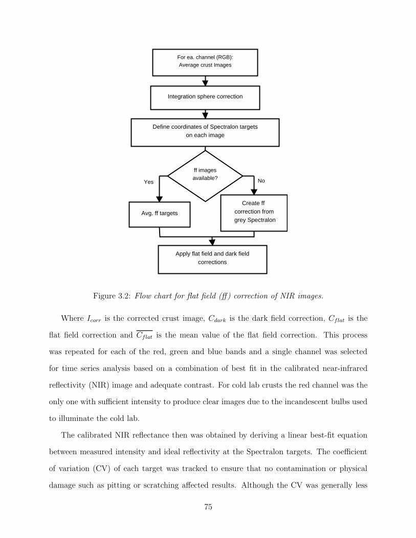
For ea. channel (RGB):Average crust Images
Integration sphere correction
Define coordinates of Spectralon targetson each image
Avg. ff targets
Create ff correction from
grey Spectralon
Apply flat field and dark fieldcorrections
ff imagesavailable?
Yes No
Figure 3.2: Flow chart for flat field (ff) correction of NIR images.
Where Icorr is the corrected crust image, Cdark is the dark field correction, Cflat is the
flat field correction and Cflat is the mean value of the flat field correction. This process
was repeated for each of the red, green and blue bands and a single channel was selected
for time series analysis based on a combination of best fit in the calibrated near-infrared
reflectivity (NIR) image and adequate contrast. For cold lab crusts the red channel was the
only one with sufficient intensity to produce clear images due to the incandescent bulbs used
to illuminate the cold lab.
The calibrated NIR reflectance then was obtained by deriving a linear best-fit equation
between measured intensity and ideal reflectivity at the Spectralon targets. The coefficient
of variation (CV) of each target was tracked to ensure that no contamination or physical
damage such as pitting or scratching affected results. Although the CV was generally less
75

than 1%, one contaminated target was identified and removed from further processing steps
in 2010. The R2 value of the linear best-fit exceeded 0.98 for all calibrated image sets,
indicating that contaminants on the targets and inhomogeneous lightning were properly
corrected before further analysis.
The calibrated reflectance images were then used to calculate the SSA using the equation
introduced by Matzl and Schneebeli (2006):
SSA = Aer/t (3.2)
Where r is the calibrated reflectance, A = 0.017 ± 0.009 mm−1, t = 12.222 ± 0.842
(R2 = 0.908) and SSA has units of mm−1. The processing steps from image correction,
to NIR calibration and calculation of SSA each introduce variability into the image array.
This may be quantified by calculating the CV for three regions of interest as an image array
is processed, shown in Figure 3.3. This is not inherently problematic, but suggests that
simply using calibrated NIR images may be more appropriate if the goal is simply to track
structural changes visually, or to obtain greater detail of snowpack layering than is possible
with traditional visible photographs.
Although the image resolution from the CMOS is approximately 0.1 mm, Matzl and
Schneebeli (2010) have shown that results using these techniques should not be extended to
the sub-millimetre scale due to concerns about light leakage between layers and subsequent
biased reflectivity measurements. Image correction and generation of NIR and SSA images
for one observation date could be accomplished in 5-10 minutes up to this point, with the bulk
of the time spent manually outlining the Spectralon targets and checking for any anomalies
in target coefficient of variation (CV).
At the conclusion of the field season and once all images for a given crust were processed,
the time series as a whole was examined for any apparent trends in morphology or variability.
Further analysis required that specific regions of interest (ROIs) be defined within each image.
Automated edge detection methods were tested in the hopes of reducing the manual input
76

averaged
corrected
NIR SSA
0
0.2
0.4
0.6
CV
of S
SA
Above CRCR_1CR_2
Figure 3.3: Increase in the coefficient of variation (CV) of SSA for 3 regions of interest atvarious points in the post-processing. The regions of interest (ROIs) include an area abovethe crust and two areas within the crust.
Figure 3.4: Example of a rejection portion of a calibrated reflectance image due to large voidsin the brittle crust as well as a gouge in the flat field correction material.
77

required, but were found to be impractical due to the occurrence of voids such as those
shown in Figure 3.4, where exposed crust surface is uneven due to crumbling when the pit
wall was cut back. The IDL iimage utility was used to graphically define ROIs in each image
using two different approaches. First, separate ROIs were defined for the crust and layers
directly above and below. Summary statistics including mean, standard deviation, range
and CV were calculated for each region of interest (ROI). The area could also be calculated
by creating a line of reference length along the snow study ruler that was included in each
NIR image. A final ROI included the crust and adjacent layers above and below. SSA values
were averaged horizontally across this ROI to create vertical profiles of SSA and variability.
The analysis of NIR imagery was refined during the summer of 2010 and crusts from
2008-09 were subsequently re-processed using the new methods. Profiles containing moist or
wet layers were problematic as Equation 3.2 was not calibrated using moist or wet snow and
free water content was only recorded as per OGRS standards (CAA, 2007) so no corrections
could be applied. Images from such days were not used in time series analyses.
3.4 Results and Discussion
Each crust was analyzed individually for temporal trends in structure and variability of
SSA as well as correlations with other characteristics such as density, grain size, average
temperature and slope-normal temperature gradient. Prior to analysing specific crusts, it is
useful to compare some representative values to those obtained during similar studies. Matzl
and Schneebeli (2006) used stereological methods to determine SSA, including six samples
classified as either ‘crust’ or ‘frozen wet grains’. Those samples yielded SSA ranging from
5 mm−1 to 20 mm−1. Domine et al. (2007) measured layers consisting of melt forms (6cl,
6mf, 8il, 9mfc per Colbeck et al. (1992)) which correspond roughly to MF and IF grain types
(from Fierz et al. (2009)) and recommended using an average value of 0.86 mm−1. Areal
averages taken from ROIs in the present study yielded values ranging from approximately 2.5
78

mm−1 to 20 mm−1, with the lowest values occurring in crusts that had undergone repeated
freeze- thaw cycles and which were comprised primarily of large clustered grains.
3.4.1 2008-09 Crusts
Three crusts were tracked during the first winter of NIR observations, all at the south-facing
same site on the South Run area of the Mt. Fidelity permanent closure. Appendix A gives
further details on the physical characteristics of the site as well as the weather contributing
to the formation of the crusts.
Figure 3.5 shows the times series of SSA for crust SR090127 as well as the layers im-
mediately above and below. As outlined in the previous section, an areal average SSA was
calculated by defining an ROI for each layer of interest for each observation date. This
crust was initially composed of two identifiable layers, with a well-bonded melt-freeze crust
overlying smaller clustered grains. The SSA of the crust is characterised by a rapid rise
during the first week of observations followed by a slow and gradual decrease until the final
observation on 11 April 2009. Thermistor data are missing during the period of the initial
increase but surface temperatures warmed to near 0 ◦C at the Mt. Fidelity weather station
and a new crust had formed on the surface at the South Run study site, so it is likely that
strong vertical temperature gradients were induced across the crust. Some weak faceting
was observed in upper portions of the crust where grains were 2-3 mm in diameter. From
10 February through 6 April the vertical temperature gradient remained weaker than 1 ◦C
10 cm−1 and the crust temperature was below freezing. From 6 April to 11 April the crust
temperature was within 0.1 ◦C of freezing, the density decreased (Appendix C) and the layer
was classified as ‘moist’, indicative of some free water. The slight increase on 11 April is
likely at least partly attributable to free water in the snowpack.
No statistically significant ( p ≤ 0.05 ) correlations were found between rates of change
of SSA and other measured parameters; however, a qualitative link appears to exist between
decreasing hand hardness and decreasing SSA.
79

0
5
10
15
20
25
SS
A [m
m−
1 ]
Feb
05
Feb
10
Feb
21
Mar
05
Mar
12
Mar
21
Mar
27
Apr 0
6
Apr 1
1
AboveCRCRBelowCR
Figure 3.5: NIR image (top) and SSA time series for crust SR090127 and adjacent layers.
80

0
5
10
15
20
25
30
SS
A [m
m−
1 ]
Feb
24
Mar
05
Mar
12
Mar
21
Mar
27
Apr 0
6
Apr 1
1
AboveCRCRBelowCR
Figure 3.6: NIR image (top) and SSA time series for crust SR090222 and adjacent layers.The ROIs used for determination of sample mean SSA are also illustrated. The largest ROIis used to calculated mean vertical profiles of SSA.
81

Crust SR090222 formed during a warm dry period in early February and was finally buried
on 22 February. Thermistors were inserted above and below the crust just after burial and
were removed at the time of the final observation on April 11. Figure 3.6 shows the time
series of mean areal SSA within the crust and in adjacent layers above and below. The
crust was initially uniform in appearance and physical characteristics, with strong bonds
that made obtaining a smooth pit wall relatively difficult. The crust remained within 50
cm of the snow surface through mid-March and vertical temperature gradients frequently
approached, though did not exceed, 1 ◦C 10 cm−1. The only apparent signal from this period
of stronger gradients was a slight increased in horizontal variability of SSA across the same
area on 5 March and some edges (indicative of faceting) on 12 March, but hand hardness
remained consistent until 6 April when the layer temperature approached 0 ◦C. As with
CR090127 the increase in SSA on 11 April is likely at least partly attributable to free water
in the snow. Strong significant ( p ≤ 0.05 ) correlations were found between SSA and the
vertical temperature gradient, but these are misleading as the actual temperature gradient
did not vary beyond the measurement accuracy of the thermocouples (0.1 ◦C) for most of
the season.
Evolution in SSA of CR090301 over one month of observations is shown in Figure 3.7.
The vertical temperature gradient underwent strong diurnal fluctuations during the first
week of March before stabilizing as the crust was buried. The increase in mean SSA from
21 March to 27 March is related to increased SSA in the lower part of the crust and a
corresponding increase in vertical CV and reduction in hand hardness. Solar insolation had
been strong for the week prior and the vertical temperature gradient had approached 1 ◦C 10
cm−1. By 6 April the crust temperature had warmed to near 0 ◦C and a strong diurnal cycle
in temperature continued until the final observation on 11 April. The large drop in SSA on
11 April is consistent with the observation that the crust structure had changed from well
bonded MFcr to large refrozen polycrystals, but may also be affected by free water in the
82

0
5
10
15
20
25
SS
A [m
m−
1 ]
Mar
05
Mar
12
Mar
21
Mar
27
Apr 0
6
Apr 1
1
AboveCRCRBelowCR
Figure 3.7: NIR image (top) and SSA time series for crust SR090301 and adjacent layers.
83

Table 3.1: Correlations of Specific Surface Area (SSA) and Near-Infrared Reflectivity (NIR)with other crust properties. TG is the vertical temperature gradient and TG96 is the 96-houraveraged vertical temperature gradient. TG* denotes the omission of CR090301.
Variable Correlation p nSSA-TG 0.69 0.001 19SSA-TG* 0.79 0.0005 15SSA-TG96 0.61 0.05 19SSA-ρ -0.46 0.04 19
NIR-Gsz -0.37 0.08 23
layer.
Given that all three crusts formed under similar meteorological conditions and were
tracked at the same site, it is worthwhile to analyze them as a group. For reference, crust
properties are tabulated in Appendix C. Table 3.4.1 shows the correlations between SSA,
NIR and other measured variables. The moderate correlation between SSA and slope-normal
temperature gradient improves somewhat if CR090301 is excluded but instantaneous tem-
perature gradient is not likely a causal factor for any trends in SSA. Lagged and average
temperature gradients were tested for correlation with SSA and rates of change and the only
statistically significant result was between the average absolute gradient over the previous
96 hours (TG96) and SSA. The negative correlation between density and SSA was also
found by Domine et al. (2007) for a range of crystal types that included crusts. The negative
correlation between NIR and grain size is expected due to the dependence of reflectivity on
grain size and the weakness is due at least in part to the difficulty in defining an ‘average’
grain size for melt-freeze layers.
A range of other physical and stability factors such as overburden mass, shear strength
at the upper boundary, compression test result and failure type and propagation saw test
(Gauthier and Jamieson, 2008) were also tested for correlation with NIR and SSA but no
significant (p ≤ 0.05) results were found.
84

Discussion: 2008-09 Natural Crusts
The first season of SSA observations included three natural melt-freeze crusts at a single
planar south-facing study site. All three crusts formed due to a combination of warm air
temperature and strong insolation, and were tracked from formation until mid-April when
all crusts because moist and bonds began to weaken (Appendix C). A number of parameters
were tested for correlation with both SSA and rates of change of SSA but few statistically
significant relationships were found. Given that the vertical, or slope-normal temperature
gradient is the primary driving force behind snowpack metamorphism a stronger correlation
with an averaged temperature gradient or a time-lagged averaged temperature gradient might
be expected. The relatively warm winter from January - April 2009 may be one factor, as all
three crusts remained within 5 ◦C, and often within 1-2 ◦C of freezing during the observation
period. This prevented the occurrence of strong temperature gradients that would drive the
formation of facets in the interior or at the boundaries of crusts. Diurnal temperature
gradients were evident by early April but several authors (e.g. Pinzer and Schneebeli, 2009)
note that diurnal gradients do not necessarily lead to faceting. The most significant structural
changes occurred at the end of the season as the crusts warmed to 0 ◦C and bonds began to
weaken, but that change was only weakly reflected in plots of areal average SSA.
Other links between SSA and physical qualities for these crusts were largely qualitative,
such as an increase in vertical variability concurrent with the weakening of bonds in por-
tions of the crust. The decreasing trend of SSA and weakening bonds in CR090127 may
provide some evidence for the importance of isothermal sintering processes (e.g Kaempfer
and Schneebeli, 2007) in melt-freeze crusts but this cannot be quantified based on the data
collected during this study.
3.4.2 2009-10 Crusts: Field
During the winter of 2009-10 six natural crusts were tracked from time of burial until mid-
April and four natural crusts were harvested, transported to a cold lab and subjected to
85
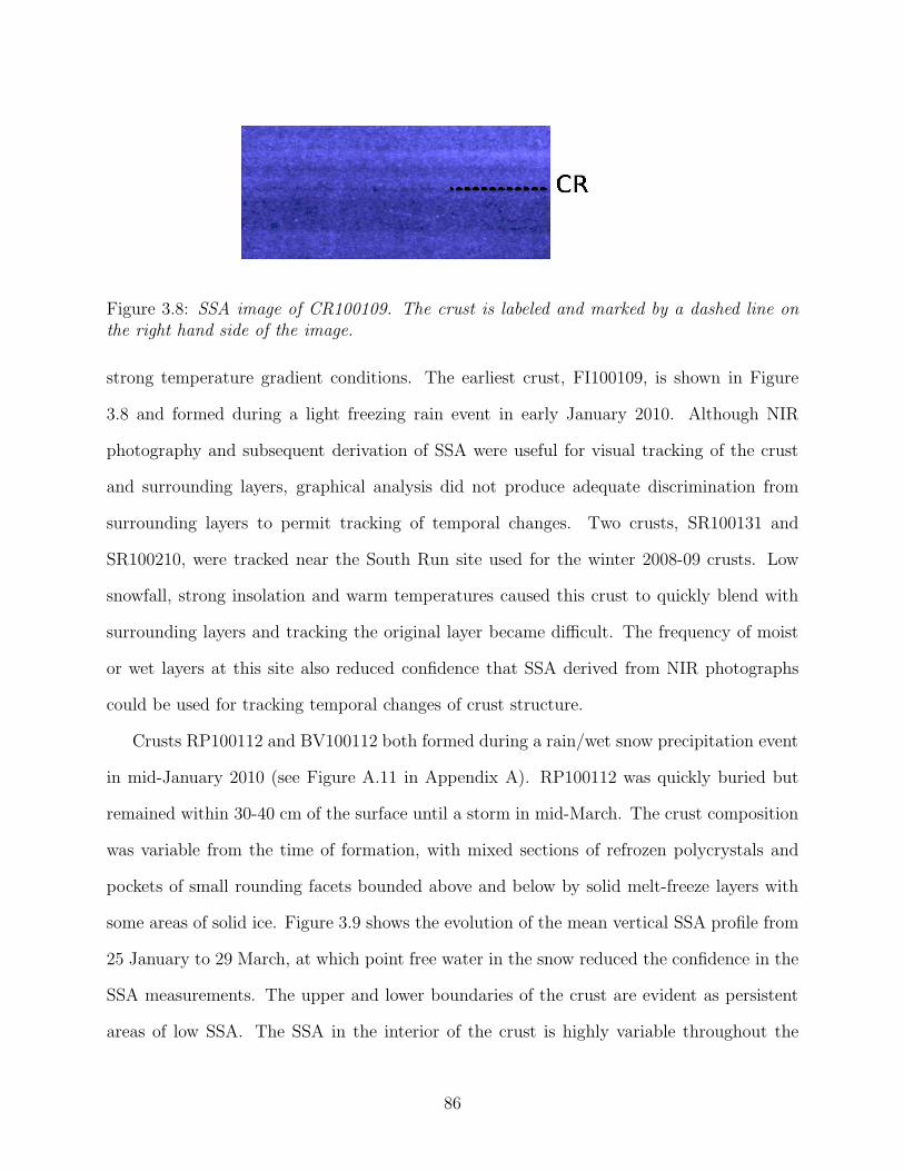
Figure 3.8: SSA image of CR100109. The crust is labeled and marked by a dashed line onthe right hand side of the image.
strong temperature gradient conditions. The earliest crust, FI100109, is shown in Figure
3.8 and formed during a light freezing rain event in early January 2010. Although NIR
photography and subsequent derivation of SSA were useful for visual tracking of the crust
and surrounding layers, graphical analysis did not produce adequate discrimination from
surrounding layers to permit tracking of temporal changes. Two crusts, SR100131 and
SR100210, were tracked near the South Run site used for the winter 2008-09 crusts. Low
snowfall, strong insolation and warm temperatures caused this crust to quickly blend with
surrounding layers and tracking the original layer became difficult. The frequency of moist
or wet layers at this site also reduced confidence that SSA derived from NIR photographs
could be used for tracking temporal changes of crust structure.
Crusts RP100112 and BV100112 both formed during a rain/wet snow precipitation event
in mid-January 2010 (see Figure A.11 in Appendix A). RP100112 was quickly buried but
remained within 30-40 cm of the surface until a storm in mid-March. The crust composition
was variable from the time of formation, with mixed sections of refrozen polycrystals and
pockets of small rounding facets bounded above and below by solid melt-freeze layers with
some areas of solid ice. Figure 3.9 shows the evolution of the mean vertical SSA profile from
25 January to 29 March, at which point free water in the snow reduced the confidence in the
SSA measurements. The upper and lower boundaries of the crust are evident as persistent
areas of low SSA. The SSA in the interior of the crust is highly variable throughout the
86

SSA 100202_RP
0 9 18 27 36 45SSA [/mm]
0
19
39
58
78
98
[mm
]
SSA 100209_RP
0 9 18 27 36 45SSA [/mm]
0
24
49
74
99
124
SSA 100215_RP
0 9 18 27 36 45SSA [/mm]
0
27
55
83
111
139
[mm
]
SSA 100227_RP
0 9 18 27 36 45SSA [/mm]
0
44
88
132
176
220SSA 100308_RP
0 9 18 27 36 45SSA [/mm]
0
24
49
73
98
122
SSA 100314_RP
0 9 18 27 36 45SSA [/mm]
0
59
119
178
238
297
[mm
]
SSA 100323_RP
0 9 18 27 36 45SSA [/mm]
0
23
46
69
92
116SSA 100329_RP
0 9 18 27 36 45SSA [/mm]
0
19
38
57
76
95[m
m]
Figure 3.9: Weekly vertical SSA profiles for crust RP100112, 25 January - 29 March, 2010.Order of evolution is left to right, top to bottom. The upper and lower boundaries of the crustare indicated by dashed lines on the first image in the series and are visible throughout asspikes of low SSA. Scale was calibrated by the inclusion of a ruler in near-infrared images.Note also that the vertical scale varies by image as regions of interest used to create thevertical profiles had to be defined manually for each set of images and were not alwaysconsistent in their upper and lower extent.
87
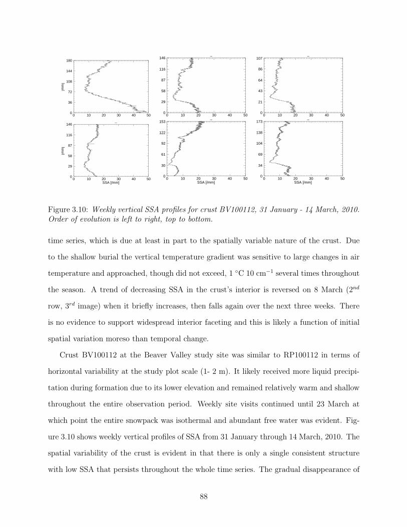
SSA 100131_Beaver
0 10 20 30 40 50SSA [/mm]
0
36
72
108
144
180[m
m]
SSA 100207_Beaver
0 10 20 30 40 50SSA [/mm]
0
29
58
87
116
146SSA 100215_Beaver
0 10 20 30 40 50SSA [/mm]
0
21
43
64
86
107
SSA 100301_Beaver
0 10 20 30 40 50SSA [/mm]
0
29
58
87
116
146
[mm
]
SSA 100308_Beaver
0 10 20 30 40 50SSA [/mm]
0
30
61
92
122
153SSA 100314_Beaver
0 10 20 30 40 50SSA [/mm]
0
34
69
104
138
173
Figure 3.10: Weekly vertical SSA profiles for crust BV100112, 31 January - 14 March, 2010.Order of evolution is left to right, top to bottom.
time series, which is due at least in part to the spatially variable nature of the crust. Due
to the shallow burial the vertical temperature gradient was sensitive to large changes in air
temperature and approached, though did not exceed, 1 ◦C 10 cm−1 several times throughout
the season. A trend of decreasing SSA in the crust’s interior is reversed on 8 March (2nd
row, 3rd image) when it briefly increases, then falls again over the next three weeks. There
is no evidence to support widespread interior faceting and this is likely a function of initial
spatial variation moreso than temporal change.
Crust BV100112 at the Beaver Valley study site was similar to RP100112 in terms of
horizontal variability at the study plot scale (1- 2 m). It likely received more liquid precipi-
tation during formation due to its lower elevation and remained relatively warm and shallow
throughout the entire observation period. Weekly site visits continued until 23 March at
which point the entire snowpack was isothermal and abundant free water was evident. Fig-
ure 3.10 shows weekly vertical profiles of SSA from 31 January through 14 March, 2010. The
spatial variability of the crust is evident in that there is only a single consistent structure
with low SSA that persists throughout the whole time series. The gradual disappearance of
88

any areas of SSA greater than 15-20 mm−1 is supported by the disappearance of any non-
melt-forms in the test profiles that were recorded concurrent with the NIR imagery, but as
with RP100112 most of the apparent change throughout the time series is likely attributable
to a high degree of spatial variation upon the crust’s formation.
Crust FI100308 was the only natural crust from winter 2009-10 that formed in a nearly
uniform manner and was buried relatively quickly. That, and the flat aspect of the study
plot at Mt. Fidelity, allows for a high degree of confidence that any observed changes were
temporal rather than due to spatial variability. Figure 3.11 shows the time series of mean
SSA for the crust and adjacent layers including a thin ice lens at the lower crust boundary.
Figure 3.12 shows vertical profiles through the crust as well as a buried surface hoar layer
from 15 March through 14 April. The profile from 9 March is not included as bright sunlight
through low density snow contaminated much of the image. The ice lens was observed on 14
April but was barely distinguishable on the vertical profile of SSA. The first profile in the
latter image is superimposed over a NIR image and illustrates one of the dangers of relying
on fully automated image processing: a drop in SSA between the crust and surface hoar
layer is caused by icy inclusions on the pit wall and, as can be seen in the following vertical
profiles, is not a consistent feature of the snowpack at the study site location.
The layer temperature of FI100308 remained between -2.5◦C and -5◦C throughout the
observation period; however, a vertical temperature gradient of approximately -1.5◦C 10
cm−1 was induced in the third week of March by the onset of colder air temperatures (Fig-
ure A.9). This gradient persisted through to the end of observations on 14 April in both
thermocouple and manual temperature measurements. Despite the gradient there was no
evidence of the structural changes that might be expected, such as faceting within the crust
or at its boundaries. Nor were there any discernible increases in the areal averaged SSA or
the vertical profiles that would be indicative of faceting.
Some evidence of relative change in SSA between the crust and adjacent layers can be
89

0
5
10
15
20
25
30
35
40
45
50
SS
A [m
m−
1 ]
Mar
09
Mar
15
Mar
22
Mar
28
Apr 0
7
Apr 1
4
AboveCRCRBelowCRIce lens
Figure 3.11: NIR image (top) and SSA time series for crust FI100308 and adjacent layersincluding a layer of buried surface hoar (SH). An ice lens at the lower crust boundary ismarked by a dashed line.
90

Figure 3.12: Weekly measurements of mean vertical SSA for crust FI100308 over one monthfrom March 15 (A) through April 14 (E). Image A shows the SSA superimposed over animage of the crust and surface hoar. The crust is outlined by dashed lines in images B - E.
91

Figure 3.13: Change in the ratio of areal averaged SSA of FI100308 to layers above andbelow.
seen by calculating the ratio of areal averages, shown in Figure 3.13. The average SSA
of FI100308 falls relative to the layers above and below from 9 March through 28 March,
hinting at either a rounding process (lower SSA) within the crust or, more likely, some slight
faceting within the layers above and below. This process reverses sharply on 7 April before
the ratios fall again on 14 April.
Stability and shear tests were not performed at Fidelity or Rogers Pass Study plots due to
space limitations, nor were they attempted at the South Run site once the two crusts became
indistinguishable from one another. Compression tests were attempted at the Beaver Valley
site but the shallow, often moist snowpack led to a high number of failures during isolation
on basal weak layers.
Discussion: 2009-10 Natural Crusts
Six natural crusts were tracked during the winter of 2009-10. The time-series observations
from two of these crusts (SR100131 and SR100210) were discarded due to the inability to
92

distinguish the crusts from one another as both remained shallow and subject to continuous
melt-freeze cycles throughout late February. A third crust, FI100109 was a very thin ice
lens and image analysis techniques used here were not adequate for tracking changes in crust
SSA, although they were effective in discriminating the thin layer from adjacent layers in
the snowpack.
Two crusts formed during a rain/wet snow event in early January and were tracked
through mid-April: RP100112 was comprised of three distinct structures that were easily
tracked in plots of vertical SSA, but were not suited to analysis using larger areas of mean
SSA as was done for the 2008-09 crusts due to internal variability even at the scale of the
pit wall. BV100112 was likewise variable upon formation. The difference in elevation and
temperature was likely the main reason for the difference in initial structure between the two
crusts and also to their variability at the scale of the study plot. Both crusts remained near
the surface but with enough of an insulation layer of snow cover to prevent the occurrence of
diurnal vertical temperature gradients. The warm air temperature in January, February and
the first half of March likewise prevented any strong vertical temperature gradients across
the crusts. Given these conditions the only changes in SSA that might be expected would
be a trend to lower SSA from melting and re-freezing into larger polycrystals. Although this
appears to be the case with BV100112, it is difficult to determine from the data whether
this is the case, or whether temporal changes were eclipsed by the initial spatial variation.
Crust FI100308 may be compared more directly with crusts SR090127 and SR090222
in that it formed at the surface during a period of warm air temperature and strong solar
insolation, then was quickly buried. Spatial variability at the snow pit scale was much
less than in BV100112 and RP100112 as would be expected from the method of formation.
Unlike other crusts from 2009-10, FI100308 remained mostly dry through mid-April and
was subjected to a weak vertical temperature gradient through the final three weeks of
observations. The slight increase in crust SSA from 28 March to 7 April may be a consequence
93

of some faceting within the crust’s interior; however no edges or faceting were found in visual
observations and the decrease from 7 April to 14 April is the opposite of what would be
observed during formation of facets. The ratio of areal mean SSA is a useful method of
quantifying relative changes in SSA between a spatially uniform crust and adjacent layers.
The increased ratio on 7 April, in conjunction with the cooling trend over the previous week
and the observation that all layers were dry, gives strength to the hypothesis that some
faceting in the crust did occur in early April.
3.4.3 2009-10 Crusts: Cold Lab
The natural crusts used in the Rogers Pass cold lab were all harvested from the same location
between 30 March and 13 April, 2010. Test profiles, NIR photography and thermal conduc-
tivity were all recorded before the crust was removed in an insulated box and transported to
the cold lab. The primary motivation was to track changes in physical properties of crusts
over relatively short periods under controlled conditions. The number of observations was
limited by the size of the insulated snow sample box shown in Figure 3.14. The cold lab
experiments were all conducted with similar ambient temperatures in the cold lab, while
varying the intervals between observations in each experiment.
Experiment LAB100330 was conducted over the course of 22 hours with a total of six
observations including one in situ before transport to the cold lab. The entire sample was
moist before it was brought into the cold lab, where the air temperature was set to -13◦C.
The crust froze slowly from the top down and was completely frozen after approximately
12 hours. Figure 3.15 shows the time series of areal average SSA of four ROIs within the
crust. The first two observations at 09:30 and 12:05 are of dubious utility as all portions of
the crust contained free water. The ‘Lower’ ROI at 14:12 is also suspect as it was not yet
frozen and some drainage of free water had occurred from upper layers.
All ROIs show similar trends in SSA, with the ‘Upper’ sample reaching its peak four
hours prior to the low layers. This is consistent with what would be expected given that
94

Figure 3.14: Schematic of the insulated box used for cold lab experiments. The front (‘Insu-lated Cover’) and sides are insulated with foam while the top is left uncovered.
upper layers were subject to strong vertical temperature gradients as soon as the sample was
brought into the lab, while deeper layers were insulated to a degree and were subject to a less-
intense and longer-lasting gradient. Thermocouples were not used during this experiment
but thermal IR images were captured at each time step immediately after the crust face
was cut back (and subsequently covered with insulation once observations were finished).
These images show that even once frozen at 21:50 the interior of the crust within 0.4 ◦C of
freezing. A recent paper by Schirmer and Jamieson (2014) has questioned the validity of
using thermal imaging for snow pit temperatures, but in this case the thermal IR imagery
is used only for qualitative evaluations of temperature and not in the identification of small-
scale variations or gradients. The SSA of all ROIs decreased between 16:55 and 21:50, then
remained approximately constant with the exception of the ‘Upper’ ROI which continued to
decrease slightly until the end of the experiment.
Experiment LAB100409 was conducted in a similar manner to LAB100330 and the cold
lab air temperature was once again set to -13◦C, but observations were evenly-spaced at
approximately 6-hour intervals and thermistors were inserted into the site of the insulated
cold lab box. Figure 3.16 shows the areal averaged SSA for ROIs in the upper, middle and
95

0
2
4
6
8
10
SS
A [m
m−
1 ]
Mar 30 09:30
Mar 30 12:05
Mar 30 14:12
Mar 30 16:55
Mar 30 21:50
Mar 31 07:24
UpperMid1Mid2Lower
Figure 3.15: NIR image (top) and SSA time series for crust LAB100330. The Upper andMid2 ROIs are visible as slightly darker areas at the top of the crust and in the middle ofthe crust, respectively.
96

0
2
4
6
8
10
SS
A [m
m−
1 ]
Apr 08 12:30
Apr 08 19:35
Apr 09 01:30
Apr 09 08:20
Apr 09 14:33
UpperMidLower
Figure 3.16: NIR image (top) and SSA time series for crust LAB100409. Portions of thecrust above the layer marked ‘Upper’ contained too many voids to ascertain the SSA withany confidence.
97

lower portions of the crust. The initial observations on 8 April at 12:30 were taken prior to
transporting the crust into the cold lab and all layers were either moist or wet.
The lowest portions of the crust froze by 23:00 but lower and middle portions continued to
cool slowly and did not reach equilibrium with the air temperature and vertical temperature
gradients greater than 1◦C 10 cm−1 persisted until the conclusion of the experiment. If the
initial observations with moist layers at 12:30 are ignored, the ROIs show a similar trend to
those in LAB100330 and all reach maximum SSA after approximately 12 hours. The SSA
of upper portion of the upper and middle portions of the crust both remain stable while the
lower portion decreases slowly over the final 12 hours.
The interval between observations was extended to 12 hours for experiment LAB100410
and all other methods including the cold lab temperature were left unchanged. The time
series of areal averaged SSA for five identifiable ROIs are shown in Figure 3.17. As with
previous cold lab experiments, the upper portion of the crust experienced strong vertical
temperature gradients immediately upon placement in the cold lab and froze first, with the
gradient dropping to below 0.1◦C 10 cm−1 14 hours after being placed in the cold lab. Lower
portions of the crust maintained a vertical temperature gradient in excess 1◦C 10 cm−1 for
24 hours and did not reach equilibrium with the cold lab air temperature until 36 hours.
Unlike the first two cold lab experiments, none of the ROIs reach a peak, and in fact the
SSA continues to decrease until the 24-hour point, remains approximately stable through 36
hours (at which point all temperature gradients were near 0 ◦C) then increased through the
next 12 hours before finally dropping again during the final observation 13 April at 09:35.
The final cold lab experiment extended the observation interval to 24 hours and the total
experiment duration to 120 hours. The cold lab temperature was set to -9◦C to slow the
freezing time and extend the duration of strong temperature gradients. The entire crust was
frozen after approximately 36 hours and the temperature of all ROIs was equalized with the
cold lab air temperature after 66 hours. Temperatures gradients greater than 1◦C 10 cm−1
98

0
2
4
6
8
10
SS
A [m
m−
1 ]
Apr 10 19:15
Apr 11 09:30
Apr 11 21:00
Apr 12 09:40
Apr 12 21:05
Apr 13 09:35
UpperMid1Mid2Mid3Lower
Figure 3.17: NIR image (top) and SSA time series for crust LAB100410. The first obser-vation 10 April at 19:15 was taken outdoors before the crust was brought into the cold lab.The area marked ‘Voids’ crumbled easily and the SSA could not be determined.
99

0
1
2
3
4
5
SS
A [m
m−
1 ]
Apr14 20:35
Apr15 21:16
Apr16 20:27
Apr17 22:05
Apr18 20:20
UpperMidLower
Figure 3.18: NIR image (top) and SSA time series for crust LAB100413.
100

persisted in lower and mid-portions of the crust for 48 hours.
Areal average SSA for LAB100413 are shown in Figure 3.18 with the backyard observa-
tions excluded. The first observation shown is for 14 April, after 24 hours in the cold lab.
The SSA of the lower ROI is a slight parabolic curve, similar to that observed over a shorter
period in the lower portion of LAB100409. The mid and lower ROIs both reach peaks at
72 hours into the experiment then decrease through the remainder. Some small developing
facets in the mid and lower ROIs were observed under a microscope on 16 April but no
observed structural changes could account for the subsequent decrease in SSA.
Discussion: 2009-10 Cold Lab Crusts
A series of four cold lab experiments were conducted at the Rogers Pass cold lab using
natural crusts harvested from the same area. All samples were moist or wet before being
brought into the cold lab and, as with other natural crusts, the validity of including SSA
measurements in time series analysis is questionable. At minimum, samples with observable
free water (‘moist’ or ’wet’) should not likely be compared with dry or fully frozen samples
if SSA is being used as a proxy for structural change in the crust.
Three of four crusts had initial increases in SSA in upper portions which were exposed
to a strong vertical temperature gradient as soon as they were placed in the cold lab. Some
development of facets and an corresponding increase in SSA would normally be expected with
melt-freeze grain types which tend to be composed of clusters of large semi-spherical grains
even when the temperature gradient is of relatively short duration (e.g. Jamieson and Fierz,
2004). LAB100410 was the sole experiment where this was not observed. Even discounting
the first observation 10 April when the crust was moist or wet, the SSA of the upper ROI
exhibits a decreasing trend. One possible explanation is that free water within this upper
layer froze in the interstitial portions of the upper ROI leading to a lower areal SSA. The
continued decrease throughout the remainder of the experiment may be attributable to the
sintering process hypothesized by Kaempfer and Schneebeli (2007).
101

LAB100410 is also anomalous due to the uniform increase of SSA in all ROIs 48 hours
into the experiment once the crust temperature was nearly equalized with the cold lab
temperature. There was no change in lighting source, diffusion of light at this time step,
nor was any shadowing evident in the NIR or visible photographs. There were also no
apparent changes in the crust structure visible under a microscope and it seems likely that
the increase due to some factor in the observational technique, but no specific reason is
immediately apparent.
It is apparent from trends in all crusts that vertical temperature gradient alone is not
reliable predictor for trends in SSA. This could be due to a number of factors including
magnitude and duration of the temperature gradients as well as the structural characteristics
of the crusts themselves, which tend to have large grains resistant to metamorphism, high
thermal conductivities and lack barriers to vertical heat transport, the opposite of what was
observed by Greene (2007).
The decrease in SSA under weak temperature gradients for LAB100413 is similar to what
was observed in the 2008-09 South Run crusts, but once again no other observations offer a
clue as to the mechanism responsible. The most likely explanation is that the natural crusts
were subject to episodic temperature gradients due to the strong diurnal cycles in the air
temperature and had already developed some internal faceting. This would be missed by
NIR photography due to the free water and then masked as the free water either refroze
or drained to lower layers and the temperature gradient disappeared as the crust reached
equilibrium with the cold lab temperature. If this hypothesis is correct, the changes are too
subtle to be tracked visually or with the aid of microscopes.
NIR photography appears to be a valid tool to track changes in crusts under artificial
conditions of the cold lab, but it is apparent that allowances have to be made for differences
in moisture content as samples are moved from a relatively warm outdoor environment into
the lab. Although various authors (e.g. Morin et al., 2010) have used NIR on layers with
102
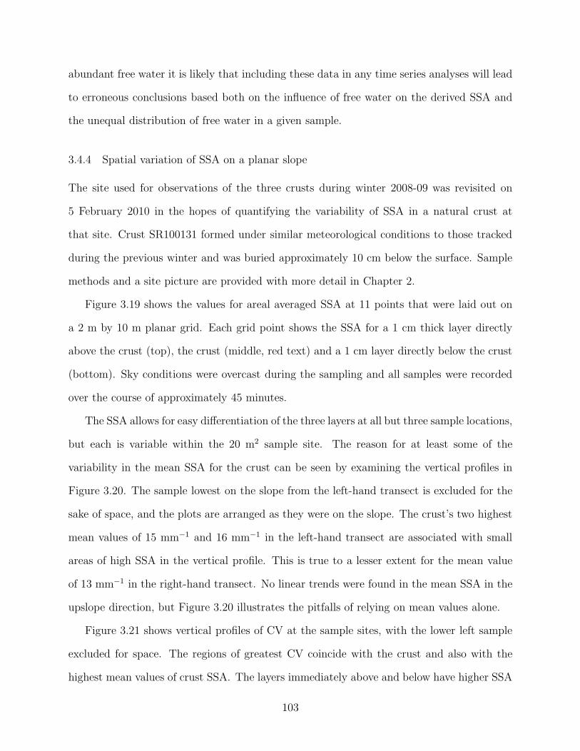
abundant free water it is likely that including these data in any time series analyses will lead
to erroneous conclusions based both on the influence of free water on the derived SSA and
the unequal distribution of free water in a given sample.
3.4.4 Spatial variation of SSA on a planar slope
The site used for observations of the three crusts during winter 2008-09 was revisited on
5 February 2010 in the hopes of quantifying the variability of SSA in a natural crust at
that site. Crust SR100131 formed under similar meteorological conditions to those tracked
during the previous winter and was buried approximately 10 cm below the surface. Sample
methods and a site picture are provided with more detail in Chapter 2.
Figure 3.19 shows the values for areal averaged SSA at 11 points that were laid out on
a 2 m by 10 m planar grid. Each grid point shows the SSA for a 1 cm thick layer directly
above the crust (top), the crust (middle, red text) and a 1 cm layer directly below the crust
(bottom). Sky conditions were overcast during the sampling and all samples were recorded
over the course of approximately 45 minutes.
The SSA allows for easy differentiation of the three layers at all but three sample locations,
but each is variable within the 20 m2 sample site. The reason for at least some of the
variability in the mean SSA for the crust can be seen by examining the vertical profiles in
Figure 3.20. The sample lowest on the slope from the left-hand transect is excluded for the
sake of space, and the plots are arranged as they were on the slope. The crust’s two highest
mean values of 15 mm−1 and 16 mm−1 in the left-hand transect are associated with small
areas of high SSA in the vertical profile. This is true to a lesser extent for the mean value
of 13 mm−1 in the right-hand transect. No linear trends were found in the mean SSA in the
upslope direction, but Figure 3.20 illustrates the pitfalls of relying on mean values alone.
Figure 3.21 shows vertical profiles of CV at the sample sites, with the lower left sample
excluded for space. The regions of greatest CV coincide with the crust and also with the
highest mean values of crust SSA. The layers immediately above and below have higher SSA
103

02
46
810
Ups
lope
dis
tanc
e [m
]
20
11
25
21
22
23
25
30
17
25
20
SSA Above [mm−1]
02
46
810
Ups
lope
dis
tanc
e [m
]
13
12
12
9
9
10
15
16
9
13
9
SSA Crust [mm−1]
2.5 2.0 1.5 1.0 0.5 0.0 −0.5
02
46
810
Cross−slope distance [m]
Ups
lope
dis
tanc
e [m
]
20
18
17
16
14
14
17
17
17
24
17
SSA Below [mm−1]
Figure 3.19: Areal SSA measurements at the planar, south-facing slope used for 2008-09crusts. The three values at each point on the slope are from a 1 cm layer above the crust,the crust (red text) and a 1 cm layer below the crust.
104
SSA 2.5
0 6 12 18 24 30SSA [/mm]
0
16
33
50
66
83
[mm
]
SSA 1.5
0 6 12 18 24 30SSA [/mm]
0
15
31
47
62
78
[mm
]
SSA 2.4
0 6 12 18 24 30SSA [/mm]
0
19
39
59
79
99
[mm
]
SSA 1.4
0 6 12 18 24 30SSA [/mm]
0
17
34
51
68
85
[mm
]
SSA 2.3
0 6 12 18 24 30SSA [/mm]
0
18
36
55
73
91
[mm
]
SSA 1.3
0 6 12 18 24 30SSA [/mm]
0
16
33
50
66
83[m
m]
SSA 2.2
0 6 12 18 24 30SSA [/mm]
0
18
37
56
75
94
[mm
]
SSA 1.2
0 6 12 18 24 30SSA [/mm]
0
16
33
50
67
84
[mm
]
SSA 2.1
0 6 12 18 24 30SSA [/mm]
0
21
42
63
84
106
[mm
]
SSA 1.1
0 6 12 18 24 30SSA [/mm]
0
16
32
48
64
81
[mm
]
Figure 3.20: Spatial variability of vertical profiles of SSA at the site used for tracking 2008-09crusts. The left column corresponds to the left-hand transect and the right column to theright-hand transect.
105

(Figure 3.19) but lower variability.
Discussion: Spatial variation of SSA
The site used for tracking of changes during the winter of 2008-09 was revisited in 2010
with the goal of quantifying spatial variation in a natural crust on a uniform slope. The
meteorological conditions of formation were solar insolation and warm air temperatures and
did not include any form of precipitation, so the crust might be assumed to be uniform on a
planar slope with no shading from vegetation. Figure 3.19 illustrates the utility in using NIR
photography for discrimination of adjacent layers, but also shows that mean SSA may vary
substantially over short distances even on uniform slopes. Figures 3.20 and 3.21 illustrate
how alternative analyses techniques may complement the areal average SSA and uncover the
reasons behind spatial variation in SSA.
As was shown with crust FI100308 the appropriate method of analysis for a given crust
will vary based on its structural characteristics. Even apparently uniform crusts may show
some variation and it is important to select a study site that will not contribute to this
variability. Each crust should be analyzed not only by its areal mean SSA but also by
vertical profiles of SSA and CV. This section illustrates the importance of considering all
methods of analysis: If only Figure 3.19 was used, the crust would seem to be more spatially
variable than it is. Once Figure 3.20 and 3.21 are considered, the reason for some of this
variation can be assigned to small areas of high SSA which of course result in a greater mean
areal SSA.
Of course some crusts such as those formed during rain-on-snow events are not well
suited for tracking of temporal changes using NIR photography due to their inherent spatial
variability. As used here, NIR photography only samples a small section and temporal
changes will likely be masked by the larger spatial variability. In these cases structural
changes should be tracked by methods using a combination of greater extent and support
(e.g.l Schweizer et al., 2008).
106

CV 2.5
0.0 0.2 0.4 0.6 0.8 1.0CV of SSA [/mm]
0
16
33
50
66
83
[mm
]
CV 1.5
0.0 0.2 0.4 0.6 0.8 1.0CV of SSA [/mm]
0
15
31
47
62
78
[mm
]
CV 2.4
0.0 0.2 0.4 0.6 0.8 1.0CV of SSA [/mm]
0
19
39
59
79
99
[mm
]
CV 1.4
0.0 0.2 0.4 0.6 0.8 1.0CV of SSA [/mm]
0
17
34
51
68
85
[mm
]
CV 2.3
0.0 0.2 0.4 0.6 0.8 1.0CV of SSA [/mm]
0
18
36
55
73
91
[mm
]
CV 1.3
0.0 0.2 0.4 0.6 0.8 1.0CV of SSA [/mm]
0
16
33
50
66
83[m
m]
CV 2.2
0.0 0.2 0.4 0.6 0.8 1.0CV of SSA [/mm]
0
18
37
56
75
94
[mm
]
CV 1.2
0.0 0.2 0.4 0.6 0.8 1.0CV of SSA [/mm]
0
16
33
50
67
84
[mm
]
CV 2.1
0.0 0.2 0.4 0.6 0.8 1.0CV of SSA [/mm]
0
21
42
63
84
106
[mm
]
CV 1.1
0.0 0.2 0.4 0.6 0.8 1.0CV of SSA [/mm]
0
16
32
48
64
81
[mm
]
Figure 3.21: Spatial variability of vertical profiles of CV of SSA at the site used for tracking2008-09 crusts. The left column corresponds to the left-hand transect and the right columnto the right-hand transect.
107

3.5 Chapter Summary
NIR photography was used derive areal mean and vertical profiles of SSA in melt-freeze
crusts over the course of two winter seasons at Rogers Pass. A total of nine natural crusts
were tracked from formation until mid-April. Four cold lab experiments were conducted by
transporting samples of natural crust into a cold lab, which was maintained at a constant
temperature for periods ranging from 12 to 120 hours. NIR observations were supplemented
with continuous temperature measurements using thermistors and thermocouples as well as
standard test profiles, which recorded grain type and size, density, hardness and temperature.
Some difficulties were encountered due to shallow crusts and anomalously warm temper-
atures during the winter of 2009-10, otherwise NIR photography techniques were found to
be simple and efficient after minimal practice. Graphical analysis of imagery proved to be
time-consuming as images had to be checked manually for pitting or scrapes along the pit
wall to ensure that they were excluded from the data set. Although imagery of adjacent
non-crust layers were captured they were not analysed during the present study.
Values and trends of SSA were compared with other observed crust properties for the
identification of any correlations or similar trends. In most cases data sets were too small to
obtain meaningful or significant correlations, but the aggregate of the three 2008-09 crusts,
all of which were formed by similar processes, revealed a moderate correlation between the
slope-normal temperature gradient and areal SSA as well as a weak correlation between
NIR reflectivity and grain size. A link between temperature gradient and SSA is expected
as the former is a major driver for snowpack metamorphism, but no correlation was found
between time-lagged or averaged temperature gradient and rates of change of SSA in either
natural crusts or cold lab crusts where the interval between observations was shorter. The
link between NIR and grain size is likewise expected due to the strong dependence of NIR
on grain size and shape. The fact that it is weak in this study is likely due to the difficulty
in defining ‘grain size’ in a well-bonded melt freeze crust.
108

No significant correlations between SSA and other crust properties were found in the
2009-10 data set; however, several apparently contradictory observations raise some questions
which may be appropriate for future research. Three of four cold lab experiments as well
as one natural crust had SSA that remained consistent or decreased despite the presence
of a vertical temperature gradient greater than 1◦C 10 cm−1, which would normally be
associated with faceting and an increase in SSA. Several observations of decreasing SSA over
time despite no observable changes in crust strength or structure hint at the importance of
microscale processes, and perhaps of destruction of weak bonds in favour of strong bonds
due to curvature effects. The presence of free water (moist or wet layers) on some dates was
problematic for analysis of time series data. The SSA equations were not validated with
this application in mind and the influence of varying percentages of free water cannot be
qualified or discounted.
An attempt was made to track the horizontal and vertical variability of SSA over time in
each crust. In some cases this proved to be successful, with trends of increasing or decreasing
variability identified, usually near the upper or lower crust boundary. In most cases this was
of limited value due to the small sample size obtained.
Finally, although well-suited for ease of operation and tracking of layers, the use of
a DSLR camera for NIR photography does present limitations in the data that may be
derived. Chief amongst those is the fact that the camera is sensitive to a broad spectrum
and results cannot be used for precise calculation of parameters such as optical diameter
and by extension cannot be used directly in radiative transfer models. Langlois et al. (2010)
employed a slightly modified technique in an attempt to overcome this limitation. Newer
methods of portable SSA measurement employed by authors such as Gallet et al. (2009) offer
more flexibility in this regard.
109

3.6 Recommendations for future studies
Results from the present study suggest improvements for future studies. NIR photography
was found to be useful both in tracking structural changes over time and in discriminating
crust layers from adjacent layers, but difficulties were encountered when layers contained free
water (classified as ‘moist’ or ‘wet’). Free water in the NIR image will affect the reflectivity
and by extension the derived SSA. There is no way to quantify the effects of free water with
the current set of observations and future studies should include quantitative measurements
of moisture content.
Temperatures in natural crusts did not vary much nor were there many instances of
strong vertical temperature gradients. Although a gradient of 1◦C 10 cm−1 is accepted as
the approximate point at which temperature gradient metamorphism becomes significant it
is likely that crusts, with high thermal conductivity, large grains and thick bonds, are more
resilient to change and require either stronger or more persistent gradients before interior
faceting occurs. For crusts that are spatially variable from time of formation there may be
utility in developing an index to quantify degree of faceting over time. It is likely that such
an index would also require larger sample sizes than were used in the present study.
Spatial variability in a relatively uniform crust is presented in Section 3.4.4. By analysing
areal average SSA and vertical profiles of SSA and CV of the SSA an accurate picture of
spatial variability may be obtained, but as outlined by Schweizer et al. (2008) tests using
only small sample areas (‘support’) may not get an accurate picture of the true variability in
a layer. Future studies should include more rigorous tests of spatial variability of a variety
of crusts including those formed from solar/air temperature effects versus those formed due
to wet snow or rain events. Such studies will by necessity be time and labor intensive due to
the destructive nature of most snowpack observations. Methods such as those used by Tape
et al. (2010) offer a good starting point for studies of spatial variability.
Analytical methods for treatment of NIR photography could be refined beyond what
110

was used in the present study. As was shown in Section 3.4.4, the mean SSA may vary
substantially across a small study plot, but relative temporal change in relation to adjacent
layers may offer valuable insight to structural changes in crusts, especially at the upper and
lower boundaries when strong vertical temperature gradients are present.
Finally, the processing of NIR imagery could likely be automated beyond what was done
in the present study. More effort in ensuring diffuse lighting and proper exposure in the field
may enable increased automation during post-processing and analysis. This was attempted
in the present study but was unsuccessful due to over or underexposure in some samples.
The most time-consuming portion of analysis involved the manual definition of specific ROIs
for each crust for each observation date.
111

Chapter 4
Snowpack Modeling
Chapter 2 and 3 introduced two relatively new methods for tracking temporal changes in
melt-freeze crusts. These measurements as well as more traditional observations of grain
type, temperature and density may be simulated using a variety of snowpack models of
varying complexity. This chapter provides a brief introduction to two physically based
models; the French CROCUS and the Swiss SNOWPACK. Five natural melt-freeze crusts
from the winters of 2008-09 and 2009-10 are simulated using the SNOWPACK model and
results are discussed along with potential improvements and recommendations for future
studies.
4.1 Literature Review
Two snowpack models are presently used in operational avalanche forecasting: SNOWPACK
(Lehning et al., 2002a,b; Bartelt and Lehning, 2002) and CROCUS (Brun et al., 1992) are
both single-column (1D) physically based models that allow evolution of microstructural and
mechanical properties of discrete layers (often referred to as ‘nodes‘) of the snowpack. The
use of some empirical parameterizations is unavoidable due to limitations in scale and gaps
in knowledge. One such case is the flux of water vapor under varying vertical (slope-normal)
temperature gradients: Metamorphism under weak macroscopic temperature gradients (eq-
uitemperature, or ‘radius of curvature’ metamorphism (Colbeck, 1980)) is dependent largely
grain size and shape, ratios of grain to bond size (Brown et al., 2001; Miller et al., 2003)
and curvature. At some point when the slope-normal temperature gradient becomes strong
enough (typically around 10 ◦C m−1) curvature effects become dominated by temperature
gradient effects (Baunach et al., 2001; Kaempfer et al., 2009). To further complicate matters
112

Sturm et al. (1997) found that vapor flux is related to grain growth rates, but they are
not directly coupled. Pinzer et al. (2012) showed that in seasonal snow subjected to high
temperature gradients of 50 ◦C m−1 the total lifetime of individual grains was on the order
of 100 hours, with longer residence times for larger or vertically oriented structures. The
same authors (Pinzer and Schneebeli, 2009) showed that alternating the direction of a strong
temperature gradient led to high recrystallization rates but not necessarily to the develop-
ment of faceted forms. The state of knowledge on metamorphism at the micro or grain scale
has advanced rapidly in recent years but such scales are smaller than what can currently be
resolved in snowpack models and metamorphism under weak or strong gradients must be
treated as discrete processes.
There has been little validation of snowpack models specifically dealing with melt-freeze
forms, though some studies have examined their influence on adjacent layers. Colbeck and
Jamieson (2001) proposed a mechanism for the formation of facets above crusts. Jamieson
and Fierz (2004) performed cold lab experiments with dry snow overlying wet snow, and
SNOWPACK was successful in reproducing the observed faceting at interface of the two
layers. Jamieson (2006) summarized the current state of knowledge regarding buried crusts,
formation of weak layers and their roles in persistent slab avalanches. Greene (2007) used ice
layers of varying thicknesses in a cold lab to test the effects of barriers to vapor flow under high
temperature gradients. Stereological analysis allowed for the retrieval of SSA and effective
bulk thermal conductivity. SNOWPACK was used to simulate the experiments and close
agreement was found between modeled and observed temperature profiles, while the bulk
thermal conductivity was generally overestimated. Smith et al. (2008) modeled the formation
and evolution of a rain-on-snow crust (CR071205) and found that the model was unable to
reproduce the formation based on meteorological inputs from a nearby weather station. Re-
initializing using an observed snow profile yielded small overestimations of temperature and
density until spring, when temperature and grain size were poorly modeled. This was likely
113

due at least in part to how the crust was initialized in the model. Rutter et al. (2009)
compared thirty-three snow cover models during simulated winter season runs using North
American Regional Reanalysis data as meteorological input, and found that such warming
events and associated drainage of free water through the snowpack were the major cause of
divergence between models.
The evaluation of model simulation of SSA and thermal conductivity is of particular
interest for this study. The temporal evolution of SSA in CROCUS may be described by
either prognostic equations based on snow age and temperature gradient (Taillandier et al.,
2007) or diagnostic equations based on either snow type and density (Domine et al., 2007)
or dendricity, grain size and sphericity (Morin et al., 2013). In the prognostic equation of
Domine et al. (2007) melt forms are assigned a constant SSA of 4.5 mm−1. Recent validation
studies (Jacobi et al., 2010; Morin et al., 2013) indicate that both routines perform relatively
well, with diagnostic equation being slightly worse due to its dependence on density. The
effective thermal conductivity is that derived by Yen et al. (1981) and is entirely a function
of density.
In SNOWPACK the optical equivalent radius is calculated as part of grain growth rou-
tines, from which the SSA may be calculated. The thermal conductivity is diagnosed as a
function of relative fractions of air, ice and water in a given layer. The conductivities of water
and ice are both dependent on temperature and an enhancement for water vapor is applied
for wet snow. Convection is not allowed, but is not likely relevant in the present study due
to the absence of long-lived sharp temperature gradients and the large voids characteristic
well developed depth hoar (Sturm and Johnson, 1992). Fierz and Lehning (2001) describe
the initial steps involved in tuning and validating grain growth and thermal conductivity
against observed values and noted that they closely followed the density-dependent equation
proposed by Sturm et al. (1997).
114

4.2 The SNOWPACK model
SNOWPACK may be driven by either measured or simulated (e.g. Bellaire et al., 2011)
meteorological data. For cold lab studies (Greene, 2007; Jamieson and Fierz, 2004) variables
such as wind and precipitation may simply be set to 0, incoming long and shortwave radiation
may be set to constants appropriate to the lab conditions and Dirichlet boundary conditions
are imposed by measured surface and basal temperatures. The minimal meteorological
inputs are air temperature, relative humidity, wind speed and direction, incoming long and
shortwave (solar) radiation and precipitation (either liquid equivalent or snow depth). The
model can also be constrained by measured surface and basal temperatures, snow depth and
measured surface albedo.
Simulations may be started before there is snow on the ground, with layers allowed to
form within the model, or the model may be initialized with a full snow profile recorded once
there is already snow on the ground. Lower boundary conditions may be set to a constant,
or the model may derive these based on meteorological inputs and ground cover (soil, grass
or snow). Rather than use IACS classifications for snow type (Fierz et al., 2009) the model
defines individual layer elements by a combination of density, grain radius, bond radius,
dendricity and sphericity. The latter two terms vary between 0 and 1, with new snow having
a dendricity of 1 and sphericity of 0, perfect rounded grains a dendricity of 0 and sphericity
of 1 and transitional (facets become rounded or vice-versa) grains a dendricity of 0. New
snow is assigned a default initial grain radius (by default 0.15 mm) and no grain growth
occurs until dendricity reaches 0. If initializing a simulation with an observed snow profile,
some trial and error is often necessary when deciding on these parameters for each existing
layer.
Figure 4.1 shows one of several matrices that are used for converting from IACS grain
types observed in snow profiles (Fierz et al., 2009) to the dendricity, sphericity and grain
size needed by SNOWPACK. Similar matrices exist for grains that have already reached
115

Figure 4.1: Matrix for converting IACS grain types to SNOWPACK grain types. Similarmatrices exist for grain types with dendricity of 0 and grains that have undergone meltingand re-freezing. From SNOWPACK documentation.
a dendricity of 0, in which case the grain in SNOWPACK is initialized using sphericity
and grain size. For layers that have undergone melting and/or refreezing the grain size and
sphericity are supplemented by a grain type marker. Markers and typical values of sphericity,
dendricity and grain size used to initialize SNOWPACK are shown in Table 4.1.
As outlined in the previous section, SNOWPACK outputs are a mixture of prognosed
and diagnosed physical properties. The former (grain and bond radius, layer density and
temperature) are physically based and are allowed to evolve throughout the course of the
simulation according the physical laws in the model. The density of new snow is based on
empirical equations and may depend on air and surface temperature, wind speed, relative
humidity and elevation, depending on the parameterization chosen by the user. Layer tem-
perature evolves based on boundary conditions in conjunction with heat transport through
adjacent layers in the snowpack. Metamorphism and density both depend on grain and bond
116

Table 4.1: Typical parameters used to initialize SNOWPACK from an observed snow profile.Abbreviations follow IACS classifications (Fierz et al., 2009). A layer of moist roundedgrains (RG) would have a marker of 12, and once refrozen would have a marker of 22.
Grain Type Dendricity Sphericity Grain Size MarkerPP 0.65-1 0-0.2 any 0DF 0.3-0.65 0-0.8 any 0FC 0 0-0.4 0-1.5 1DH 0 0-0.5 ≥1.5 1RG 0-0.1 0.5-1 0-0.7 2
RGxf/FCxr 0 0.2-0.8 0-1 2SH 0 0 any 3
Moist or Wet 0 0-1 any +10Refrozen (MF) 0 0-1 any +10
radii, dendricity, sphericity, microstructure marker, coordination number, thermal conduc-
tivity and viscosity. The transition between equitemperature (EQ) and temperature gradient
(TG) metamorphism is defined explicitly in terms of the vapour pressure gradient and is by
default 5 hPa m−1.
Other parameters such as optical equivalent grain size, effective thermal conductivity,
layer hardness are diagnosed at each time step after metamorphism has occurred. Some,
such as hardness, are calculated only for evaluation purposes while others such as thermal
conductivity and optical radius are carried forward to the next time step for use in thermal
and metamorphic routines.
Version 3.2 of SNOWPACK, used in this study, incorporates a number of recent for-
mulations for thermal conductivity, equivalent optical diameter and water transport (e.g.
Hirashima et al., 2008, 2010). This latest version was selected due to the relative abundance
of recent research that has been incorporated from snow climates around the world, whereas
older versions had often been validated primarily in the Swiss Alps.
The optical equivalent diameter in the near-infrared band in SNOWPACK is derived by
117

an empirical equation published in Vionnet et al. (2012) where for non-dendritic forms,
dopt = 2 ∗ (0.5 ∗ (2 ∗ rg ∗ s + (1− s) ∗max(0.4, rg)) (4.1)
where dopt has units of mm, rg is the model grain radius and 0 < s < 1 is the model
sphericity, which varies from 0.0 for new snow to 1.0 for perfectly rounded crystals. For
grains with a sphericity of 1.0 the optical diameter is equal to the physical diameter. To
compare with field measurements of SSA, the transform published by Matzl and Schneebeli
(2006) may be used;
dopt =6
SSA(4.2)
where dopt has units of mm and SSA has units of mm−1. Due to the uncertainty in
spectral response of the camera used to capture NIR images in this study as well as well as
in the equation used to determine the SSA (Chapter 3) this is not an exact relationship but
will still give a relative measure of model performance.
Thermal conductivity for very high or very low density snow is defined as a linear combi-
nation of thermal conductivity of the volumetric fractions of ice, air and water for each layer.
For snow of intermediate density a more complex empirical equation is used which incor-
porates wind pumping, water vapor in pore spaces and temperature dependence of thermal
conductivities of ice and water fractions.
For hand hardness, SNOWPACK has three available parameterizations for hand hard-
ness, all of which output a hardness index from 1 - 6 per the International Classification
of Seasonal Snow on the Ground (Fierz et al., 2009). The default configuration (MONTI)
assigns a hardness based on grain type and density with lower index values with increas-
ing water content. Fully frozen melt-freeze forms are assigned a constant value of 5; the
Swiss parameterization depends only on grain size and density except in the case of melt
forms, when the index is reduced with increasing water content; the ASARC parameteriza-
tion is based on a regression on the ASARC database from 2002 and depends on grain type
118

and density for new snow and surface hoar. Grain size is incorporated for other forms as
well as water content for melt forms. The hardness may be converted to Swiss Ramsonde
penetration resistance for output using the formula
RN = 19.3 ∗R2.4index (4.3)
where RN is in units of Newtons. Calibrated vertical penetration resistance should not be
directly compared to the horizontal resistance recorded in test profiles following the standards
in CAA (2007) but the two are likely monotonically related.
SNOWPACK may be used to simulate multiple aspects starting either from bare ground
or by initializing the model using both a flat-field profile and profiles from each aspect to
be simulated. In this case the snow cover is allowed to evolve independently on each aspect
based on meteorological data from the flat-field weather station, and snow transport by wind
may also be simulated from one aspect to another.
4.3 SNOWPACK Simulations
Five natural crusts from winters 2008-09 and 2009-10 were simulated using SNOWPACK
version 3.2, which was released in February 2014 and incorporated significant changes from
past versions including an improved water transport scheme (Hirashima et al., 2010). Two
of these were natural crusts at Mount Fidelity study plot and the remaining three were from
the South Run area of Mount Fidelity closure. The crusts were chosen due to their relative
homogeneity as being more suitable to simulation by a single column model that by its
nature cannot incorporate spatial variability over the scale of a study plot. A rain crust from
December 2007 that was simulated with an older version of SNOWPACK (Smith et al., 2008)
was not revisited due to its spatial variability and the conclusion that formation could not be
simulated using only surface meteorological measurements. Several crusts from winter 2009-
10 were not simulated due to a lack of input meteorological data (RP100112, BV100112) and
119

difficulty in tracking the crusts due to constant melting and merging (SR100131, SR100210).
Model data were extracted from SNOWPACK output files and plotted alongside ob-
servations of layer depth, density, temperature, SSA and, for 2010, thermal conductivity.
Evaluation of a thin rain crust (FI100109) was limited to qualitative evaluation of forma-
tion and thickness as the layer was too thin for reliable measurements of SSA, density and
thermal conductivity.
4.3.1 SNOWPACK configuration
Meteorological data from Mount Fidelity station, described in Appendix A, were used to
drive simulations for all natural crusts. Hourly data at the station were supplied by a venti-
lated incoming pyranometer and incoming longwave radiometer, wind speed and direction,
air temperature, relative humidity and a precipitation accumulator with resolution of 0.1
mm. Hourly measurements of new snow accumulation on a 24-hr snow board, cleared ap-
proximately daily, were used by Bellaire et al. (2011) but were not used to constrain model
snow depth in these simulations. Data were logged on a Campbell CR10X datalogger pow-
ered by batteries, which typically ran down over the summer so data were not available until
the first site visit of the winter season in late November or early December.
Simulations were initialized using full depth profiles (CAA, 2007) observed by Parks
Canada avalanche technicians or from ASARC researchers. All model runs were config-
ured with neutral atmospheric stability, Neumann boundary conditions and with the canopy
model disabled as all study sites were in open areas. Default model parameterizations were
used for surface albedo, new snow density and layer hardness. Some other options were
modified to provide better agreement between modeled output and observations; these are
detailed in the next section.
120

4.3.2 South Run 2009 Crusts
Three natural melt-freeze crusts (SR090127, SR090222 and SR090301) were tracked at the
South Run area of the Mount Fidelity study area during the winter of 2008-09. The study
plot is approximately 700 m from the Fidelity weather station on a south-southeast aspect.
As outlined in Appendix A, a failure of the Fidelity datalogger led to a loss of radiation
data from 20 February - 5 March so simulation of a complete winter’s snowpack was not
possible. Specific Surface Area measurements are described more completely in Chapter 3
and thermal conductivity data were not collected during the winter of 2008-09.
Simulations of the South Run crusts were initialized using a Parks Canada full profile at
Mount Fidelity from 2 March and ASARC test profiles at Fidelity and South Run from 5
March. The South Run test profile extended to 20 cm below SR090127 and the remainder
of the profile was artificially populated with rounded grains. The two profiles at Fidelity
were merged into a synthetic ‘full profile‘. The developers of SNOWPACK note that this
approach is less ideal than allowing all layers to form naturally. The initialization of melt-
freeze crusts presents some unique difficulties since grain and bond size are not well-defined
or easily measured.
Snow erosion and snow distribution routines were enabled, the canopy model was disabled
and other parameterizations were left at their default configurations for the initial run with a
60 minute timestep. This first configuration led to a lack of convergence in the temperature
subroutines, possibly due to strong insolation and warming. The timestep was subsequently
reduced to 15 minutes with meteorological data resampled from the original 60 minute
intervals. Resampling is done automatically by the MeteoIO library, which is used to process
input data for SNOWPACK version 3.2. The three simulations run for these crusts are
summarized in Table 4.2.
Evolution of grain type and snow depth from this first simulation SR20090305-1, are
shown in Figure 4.2. A period of accumulation from early to late March followed by rapid
121

Table 4.2: SNOWPACK iterations for SR20090305.
Run Name Parameters modified Modified valueSR20090305-1 none model defaultsSR20090305-2 crust grain size optical diameter from SSASR20090305-3 water transport NIED
warming and settling is evident, as is the rapid warming of the upper snowpack by April 11,
denoted by a region of solid red. The three crusts of interest exist at the start of the run
shortly after SR090301 was first buried.
The simulated and observed depth of the top of each crust is shown in Figure 4.3. SNOW-
PACK’s simulated depths are very close to measured depths with the exception of 21 March,
when the simulated depth is 10-20 cm shallower than observed depth for all crusts. Referring
to Figure 4.2 it appears that actual snow accumulation exceeded simulated accumulation.
The simulated depth for SR090127 on 27 March is greater than was observed indicating
insufficient settling in upper midpack layers.
Figure 4.4 shows simulated and measured density and temperature for crust SR090127.
Minimum and maximum values from SNOWPACK are due to the the model treating layers
as multiple discrete nodes so there is often a range of physical properties that correspond to
a single ‘layer‘ in an observed snow profile. There is a marked negative temperature bias in
the simulation until the snow becomes isothermal on 11 April. The simulated density tracks
closely with observations until 27 March when the observed density spikes. The observed
temperature on March 27 was -0.8 ◦C and although the crust was classified as ‘dry‘ it is
likely that the increased density was related to these warmer temperatures which were not
replicated by SNOWPACK.
Figure 4.5 shows the simulated and observed SSA for SR090127, where the simulated
SSA are derived from the model optical diameter using Equation 4.2. There are multiple
sources of error in the measurements including errors in the SSA parameterization, spatial
122

New Snow Decomposing
Rounding
DecomposedFaceting
Rounded
Faceting
Faceted
Moist rounds
Moist facetsV. Faceted
Wet rounds
Wet facetsDepth Hoar
Ice lens
Surface hoar
Frozen crust
250
150
50
Heig
ht
(cm
)
Figure 4.2: Evolution of snow depth (cm) and grain type for simulation SR20090305-1 runfrom 5 March - 11 April, 2010. Melt-freeze crusts are denoted by red with vertical cyan linesand moist or wet layers by solid red shading. New snow is shaded green and rounded grainsare shaded pink.
123

0
10
20
30
40
50
60
70
80
90
100
Laye
r D
epth
[cm
]
ObservedSNOWPACK
0
10
20
30
40
50
60
70
80
90
100
Laye
r D
epth
[cm
]
ObservedSNOWPACK
03/0
5 11
:15
03/1
2 10
:40
03/2
1 09
:30
03/2
7 10
:30
04/0
6 10
:30
04/1
1 11
:00
50
60
70
80
90
100
110
120
130
140
150
Laye
r D
epth
[cm
]
ObservedSNOWPACK
Figure 4.3: Modeled versus observed layer depth for SR090301 (top), SR090222 (middle)and SR090127 (bottom) from run SR20090305-1.
124

200
250
300
350
400
Laye
r D
ensi
ty [
kg m
−3 ]
ObservedSNOWPACK_minSNOWPACK_max
03/0
5 11
:15
03/1
2 10
:40
03/2
1 09
:30
03/2
7 10
:30
04/0
6 10
:30
04/1
1 11
:00
−5
−4
−3
−2
−1
0
Laye
r Te
mpe
ratu
re [
o C]
ObservedSNOWPACK_minSNOWPACK_max
Figure 4.4: Measured versus simulated layer density (top) and layer temperature (bottom)for SR090127 from run SR20090305-1.
125
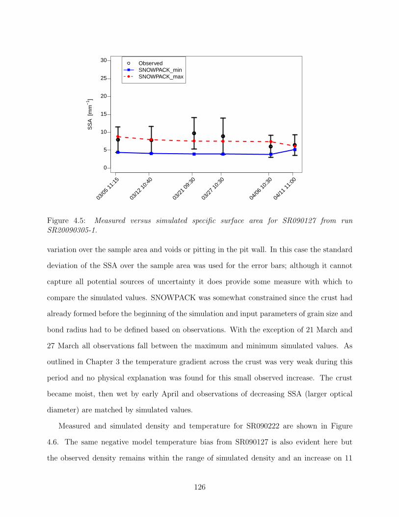
03/0
5 11
:15
03/1
2 10
:40
03/2
1 09
:30
03/2
7 10
:30
04/0
6 10
:30
04/1
1 11
:00
0
5
10
15
20
25
30
SS
A [
mm
−1 ]
ObservedSNOWPACK_minSNOWPACK_max
Figure 4.5: Measured versus simulated specific surface area for SR090127 from runSR20090305-1.
variation over the sample area and voids or pitting in the pit wall. In this case the standard
deviation of the SSA over the sample area was used for the error bars; although it cannot
capture all potential sources of uncertainty it does provide some measure with which to
compare the simulated values. SNOWPACK was somewhat constrained since the crust had
already formed before the beginning of the simulation and input parameters of grain size and
bond radius had to be defined based on observations. With the exception of 21 March and
27 March all observations fall between the maximum and minimum simulated values. As
outlined in Chapter 3 the temperature gradient across the crust was very weak during this
period and no physical explanation was found for this small observed increase. The crust
became moist, then wet by early April and observations of decreasing SSA (larger optical
diameter) are matched by simulated values.
Measured and simulated density and temperature for SR090222 are shown in Figure
4.6. The same negative model temperature bias from SR090127 is also evident here but
the observed density remains within the range of simulated density and an increase on 11
126

April is accurately modeled. A comparison of SSA is given in Figure 4.7. There is a large
difference even at the start of the simulation, reflecting the difference between observed
grain size and SNOWPACK’s treatment of grain size for melt-freeze crusts. Despite this,
observations converge with simulated SSA by 6 April when the crust became moist and grain
size increased.
Measured and simulated density and temperature for SR090301 are shown in Figure 4.8
and SSA in Figure 4.9. The observed density is generally within the bounds of simulated
density for the layer except for 6 April, where the observed density increased sooner than the
simulated density. The simulated layer temperature is once again colder than observations
until isothermal conditions were reached by 11 April. Like SR090127, the simulated SSA
tracks closely with the observations and accurately captures the decrease once the layer
became moist and then wet in April.
Simulation SR20090305-2 was identical to SR20090305-1 except that all three crusts were
initialized using the optical diameter derived from the observed SSA on 5 March rather than
the observed grain size. The time series of simulated versus observed SSA for all three crusts
is shown in Figure 4.10. The simulated SSA on 5 March does not exactly match observations
because the crusts were assigned a sphericity of 0.9 so the physical diameter does not quite
correspond to the optical diameter and SSA.
In the case of SR090301 the new initialization actually leads to a slightly greater spread
in simulated SSA, with the same general trend in values and sharp decrease in April. The
difference between the grain size from field observations and that derived from SSA on
5 March was small so this is not surprising. For SR090222 the difference in initialized
grain size between the two simulations is large, and the new simulation tracks much closer
to observations until late March, when the observed SSA decreased faster than simulated
values. This could be an artifact of the cold temperature bias in the model.
SR090127 was initially composed of two identifiable layers, with an upper portion com-
127
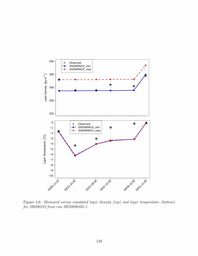
200
250
300
350
400
Laye
r D
ensi
ty [
kg m
−3 ]
ObservedSNOWPACK_minSNOWPACK_max
03/0
5 11
:15
03/1
2 10
:40
03/2
1 09
:30
03/2
7 10
:30
04/0
6 10
:30
04/1
1 11
:00
−10
−9
−8
−7
−6
−5
−4
−3
−2
−1
0
Laye
r Te
mpe
ratu
re [
o C]
ObservedSNOWPACK_minSNOWPACK_max
Figure 4.6: Measured versus simulated layer density (top) and layer temperature (bottom)for SR090222 from run SR20090305-1.
128

03/0
5 11
:15
03/1
2 10
:40
03/2
1 09
:30
03/2
7 10
:30
04/0
6 10
:30
04/1
1 11
:00
0
5
10
15
20
25
30
SS
A [
mm
−1 ]
ObservedSNOWPACK_minSNOWPACK_max
Figure 4.7: Measured versus simulated specific surface area for SR090222 from runSR20090305-1.
posed of smaller grains and the lower portion having larger grains. This was reflected in
the results from SR20090305-1 where simulated SSA was based in initialization from ob-
served grain size, but the use of observed SSA removes this distinction and as a result the
spread in simulated values is very small until 11 April. The general trend in observations is
well-modeled but observed SSA did decrease slightly earlier than simulated SSA.
The simulated temperature, layer depth and layer density did not change with the new
initialization and are not shown here. The third simulation, SR20090305-3 used the same
initialization as SR20090305-1 except that the Japanese NIED snow water transport model
was used instead of the default Bucket model. In this case warming and layer wetting
occurred much too soon, to a greater degree and extended much deeper than was observed.
Since performance using this routine was poor, the results are not shown here.
The final parameter evaluated is the hand hardness. As explained in Section 4.2 the
default routine in SNOWPACK sets the hardness of frozen melt forms to 5, with decreased
hardness assigned with increasing water content while the ASARC routine incorporates den-
129
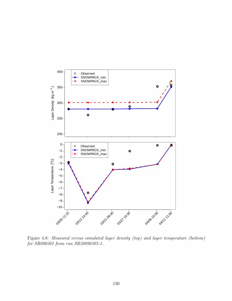
200
250
300
350
400
Laye
r D
ensi
ty [
kg m
−3 ]
ObservedSNOWPACK_minSNOWPACK_max
03/0
5 11
:15
03/1
2 10
:40
03/2
1 09
:30
03/2
7 10
:30
04/0
6 10
:30
04/1
1 11
:00
−10
−9
−8
−7
−6
−5
−4
−3
−2
−1
0
Laye
r Te
mpe
ratu
re [
o C]
ObservedSNOWPACK_minSNOWPACK_max
Figure 4.8: Measured versus simulated layer density (top) and layer temperature (bottom)for SR090301 from run SR20090305-1.
130

03/0
5 11
:15
03/1
2 10
:40
03/2
1 09
:30
03/2
7 10
:30
04/0
6 10
:30
04/1
1 11
:00
0
5
10
15
20
25
30
SS
A [
mm
−1 ]
ObservedSNOWPACK_minSNOWPACK_max
Figure 4.9: Measured versus simulated specific surface area for SR090301 from runSR20090305-1.
sity. Field observations of hand hardness were converted to index values using tabular data
in Fierz et al. (2009). It should be emphasized that observations of hand hardness are sub-
ject to variability due both to differences between observers and the relatively imprecise
methods used to record them. If a given layer is not isotropic then simulated values given
in SNOWPACK may not correspond to those observed in the field.
Figure 4.11 shows the observed hand hardness compared with simulated values using the
default MONTI routine as well as the ASARC routine. The ASARC routine underestimates
hardness until the crusts became moist at which point it accurately captured both hardness
and the decrease in hardness between 6 April and 11 April. The default MONTI parame-
terization was more accurate while the crusts remained frozen but grossly overestimated the
decrease in hardness for SR090301 and SR090222 between 6 April and 11 April. The cold
bias in the model seen for all three crusts was likely a factor as crusts became moist and lost
strength sooner than they did in the simulations.
131

0
5
10
15
20
25
30
SS
A [
mm
−1 ]
ObservedSNOWPACK_minSNOWPACK_max
0
5
10
15
20
25
30
SS
A [
mm
−1 ]
ObservedSNOWPACK_minSNOWPACK_max
03/0
5 11
:15
03/1
2 10
:40
03/2
1 09
:30
03/2
7 10
:30
04/0
6 10
:30
04/1
1 11
:00
0
5
10
15
20
25
30
SS
A [
mm
−1 ]
ObservedSNOWPACK_minSNOWPACK_max
Figure 4.10: Measured versus simulated specific surface area for SR090301 (top), SR090222(middle) and SR090127 (bottom) from run SR20090305-2. Crust grain size was initializedusing optical diameter derived from SSA measurements.
132

1
2
3
4
5
6
Har
dnes
s In
dex
ObservedSNOWPACK_montiSNOWPACK_asarc
1
2
3
4
5
6
Har
dnes
s In
dex
ObservedSNOWPACK_montiSNOWPACK_asarc
03/0
5 11
:15
03/1
2 10
:40
03/2
1 09
:30
03/2
7 10
:30
04/0
6 10
:30
04/1
1 11
:00
1
2
3
4
5
6
Har
dnes
s In
dex
ObservedSNOWPACK_montiSNOWPACK_asarc
Figure 4.11: Hardness index for SR090301 (top), SR090222 (middle) and SR090127 (bottom)from simulation SR20090305-1.
133

4.3.3 South Run 2009 Crusts Discussion
SNOWPACK simulations of crusts SR090127, SR090222 and SR090301 on a simulated south-
facing slope revealed a cold bias in the model that persisted until the final observation on
11 April when all three layers had become isothermal. This temperature bias was likely the
most important contributing factor to errors in layer depth and for the lag between increases
in observed and simulated density for SR090301 and SR090222. This lag was not observed
in SR090222 but it also had generally higher densities than the other two crusts and may
not be expected to increase in density quite as quickly with small increases in water content.
There are several possible reasons for the temperature bias, including model albedo being
too high and overprediction of nighttime cooling. It is also possible that measured incoming
solar radiation at Mount Fidelity was not representative of South Run. Although the two
sites are separated by only 700 m, South Run faces the intersection of two large valleys while
Fidelity lies just downstream of the convergence zone: when clouds formed due to orographic
lift it was quite possible to have different sky conditions at the two sites.
Hand hardness was modeled relatively well using the default hardness routine in SNOW-
PACK, but not as well once layers became moist and lost strength. The cold bias in the
model is likely at least a contributing factor to this discrepancy. The ASARC hardness
routine, which incorporates density for frozen melt forms, underestimated hardness until
the layers became moist or wet, at which point it became a better predictor of the actual
hardness as well as the decrease in hardness due to layer wetting. It should be noted that
the MONTI routine does include a density-dependent equation for hardness of dry or moist
melt-freeze forms but it is not used in the present version of SNOWPACK.
The simulation of trends in SSA is generally good in SNOWPACK, especially as grain
coarsening occurred with springtime wetting and diurnal melt-freeze cycles. The largest
limitation was with the initialization of crusts using observed grain size, which is not well-
defined for melt-freeze forms and does not necessarily correspond to how grain size and
134

bond radius are treated in SNOWPACK. In this case using an optical diameter derived from
measured SSA gave better results. Some thought for other initialization parameters such as
sphericity and bond radius is still required as they will affect the rate of grain growth and
thermal conductivity. This approach was not tested for adjacent layers but it is possible that
this approach could offer improvements for situations when simulations cannot be started
with bare ground.
4.3.4 FI100308
The simulation for FI100308 was initialized from a full profile recorded by Parks Canada
avalanche technicians on 8 December, 2009 and was run until the final ASARC profile on 14
April, 2010. The study site was immediately adjacent to the meteorological instrumentation
on flat terrain, and was sheltered from all but North winds so was rarely subject to snow
drifting. Exposure to solar radiation was uniform across the entire study plot. Unlike
simulations for South Run crusts in 2008-09, meteorological data were available beginning
in early December 2009 and both crusts of interest were allowed to form naturally rather
than being explicitly defined.
Both FI100308 and FI100109 were of interest for this simulation, but simulations of
the latter are only evaluated based on whether or not it forms. Table 4.3 summarizes the
three simulations that were run. FI100109 did not form during FI20091208-1, but did once
threshold temperature between rain and snow was increased from -0.5 ◦C to 0.9 ◦C for
simulation FI20091208-2. This was likely a limitation due to lack of surface temperature
measurements as the skin temperature must then be calculated using a combination of
measured air temperature and incoming solar and longwave radiation. This is an important
consideration for future work involving numerical weather models as their current ability
to prognose skin temperature is relatively poor. For simulation FI20091208-3 the water
transport parameterization was changed to the newer NIED formulation (Hirashima et al.,
2010) but the timing and depth of wetting was much greater than what was observed. The
135

Table 4.3: SNOWPACK iterations for FI20091208.
Run Name Parameters modified Modified valueFI20091208-1 none defaultsFI20091208-2 rain-snow threshold increase by 1.4 ◦CFI20091208-3 water transport NIED
remainder of this section presents only results from FI20091208-2.
Evolution of grain type and accumulation of new snow for the entire simulation, from 8
December, 2009 to 14 April, 2010, is shown in Figure 4.12. Crust FI100109 can be seen to
form and become quickly buried in early January, but this was achieved only by tuning the
model threshold between rain and snow to observed air temperature and precipitation in the
meteorological inputs. Had measurements of surface temperature been available this tuning
may not have been necessary. Crust FI100308 is visible as the first thick crust to form,
approximately two thirds of the way through the simulation. Like FI100109 it is quickly
buried and does not become wetted by the end of the simulation.
Figure 4.13 shows the comparison between observed and simulated snow depth, layer
depth and layer temperature beginning with the first observation of FI100308 on March 9,
2010. The simulation had been allowed to run for three months up to this point with no
nudging of surface temperature or snow depth; new snow layers were created entirely by
the snowpack model and based only on meteorological inputs. The simulated snow depth is
remarkably close to observations, with a slight underprediction in early April when simulated
new snow layers were slightly too dense and settlement occurred too quickly. The same
pattern is evident in the depth of the top of FI100308. Both snow depth and layer depth
were correct for the first observation on 9 March and the larger discrepancies are associated
with increasing downwelling solar radiation and a week-long cold spell in late March and
early April (see A for more detail on meteorological data).
Simulated layer temperatures exhibit a warm bias but are still within 1 ◦C. This is in
136
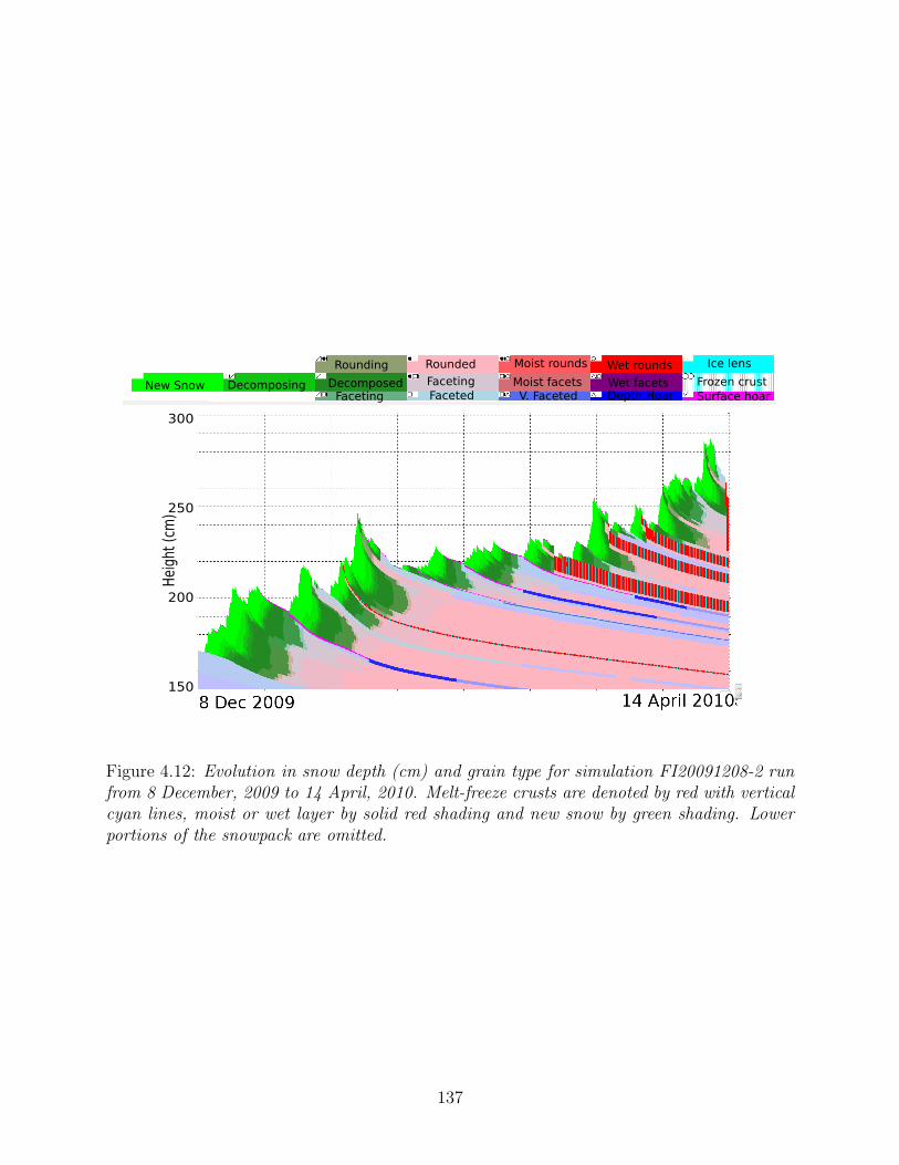
New Snow Decomposing
Rounding
DecomposedFaceting
Rounded
Faceting
Faceted
Moist rounds
Moist facetsV. Faceted
Wet rounds
Wet facetsDepth Hoar
Ice lens
Surface hoar
Frozen crust
300
250
200
150
300
250
200
150
Hei
ght
(cm
)
Figure 4.12: Evolution in snow depth (cm) and grain type for simulation FI20091208-2 runfrom 8 December, 2009 to 14 April, 2010. Melt-freeze crusts are denoted by red with verticalcyan lines, moist or wet layer by solid red shading and new snow by green shading. Lowerportions of the snowpack are omitted.
137
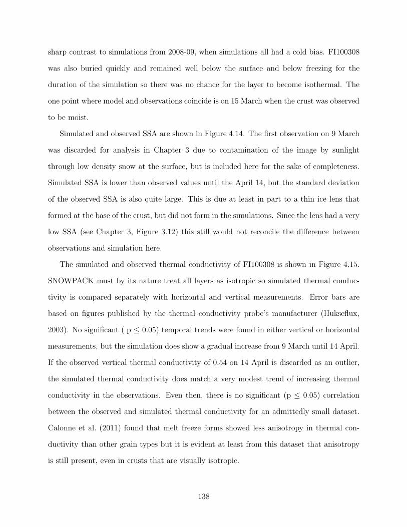
sharp contrast to simulations from 2008-09, when simulations all had a cold bias. FI100308
was also buried quickly and remained well below the surface and below freezing for the
duration of the simulation so there was no chance for the layer to become isothermal. The
one point where model and observations coincide is on 15 March when the crust was observed
to be moist.
Simulated and observed SSA are shown in Figure 4.14. The first observation on 9 March
was discarded for analysis in Chapter 3 due to contamination of the image by sunlight
through low density snow at the surface, but is included here for the sake of completeness.
Simulated SSA is lower than observed values until the April 14, but the standard deviation
of the observed SSA is also quite large. This is due at least in part to a thin ice lens that
formed at the base of the crust, but did not form in the simulations. Since the lens had a very
low SSA (see Chapter 3, Figure 3.12) this still would not reconcile the difference between
observations and simulation here.
The simulated and observed thermal conductivity of FI100308 is shown in Figure 4.15.
SNOWPACK must by its nature treat all layers as isotropic so simulated thermal conduc-
tivity is compared separately with horizontal and vertical measurements. Error bars are
based on figures published by the thermal conductivity probe’s manufacturer (Hukseflux,
2003). No significant ( p ≤ 0.05) temporal trends were found in either vertical or horizontal
measurements, but the simulation does show a gradual increase from 9 March until 14 April.
If the observed vertical thermal conductivity of 0.54 on 14 April is discarded as an outlier,
the simulated thermal conductivity does match a very modest trend of increasing thermal
conductivity in the observations. Even then, there is no significant (p ≤ 0.05) correlation
between the observed and simulated thermal conductivity for an admittedly small dataset.
Calonne et al. (2011) found that melt freeze forms showed less anisotropy in thermal con-
ductivity than other grain types but it is evident at least from this dataset that anisotropy
is still present, even in crusts that are visually isotropic.
138

220
230
240
250
260
270
280
Sno
w D
epth
[cm
]
ObservedSNOWPACK
0
10
20
30
40
50
60
70
80
90
100
Laye
r D
epth
[cm
]
ObservedSNOWPACK
03/0
9 12
:30
03/1
5 15
:30
03/2
2 15
:30
03/2
8 15
:30
04/0
7 15
:30
04/1
4 06
:30
−5
−4
−3
−2
−1
0
Laye
r Te
mpe
ratu
re [
o C]
ObservedSNOWPACK_minSNOWPACK_max
Figure 4.13: Measured versus simulated snow depth, layer depth and layer temperature forcrust FI100308 from simulation FI20091208-2.
139

03/0
9 12
:30
03/1
5 15
:30
03/2
2 15
:30
03/2
8 15
:30
04/0
7 15
:30
04/1
4 06
:30
0
5
10
15
20
25
30
SS
A [
mm
−1 ]
ObservedSNOWPACK_minSNOWPACK_max
Figure 4.14: Measured versus simulated specific surface area for FI100308 from simulationFI20091208-2.
4.3.5 FI100308 Discussion
Two crusts from the winter of 2009-10 were simulated starting from 8 December and running
until 14 April. The earlier crust, FI100109, did not form in the simulation using default
model settings. When the model threshold was increased so that SNOWPACK produced
rain rather than snow the layer did form, albeit thicker than was observed. It is possible
that if surface temperature measurements were available that the crust would have formed
as observed. This does illustrate the difficulty of diagnosing precipitation type using only
surface observations, when above freezing layers may produce rain or freezing rain while the
surface air temperature remains below 0 ◦C. A similar synoptic environment was present
during the formation of thick rain crust in December 2007 and, lacking that information,
SNOWPACK interpreted the precipitation as snow rather than rain.
Total snowpack height and depth of crust FI100308 were very well simulated especially
considering that the first field observations occurred three months into the simulation. Sim-
ulated snowfall settled slightly too quickly from mid-March until early April with the largest
140

0
0.1
0.2
0.3
0.4
0.5
0.6
The
rmal
Con
duct
ivity
[W
m−
1 K−
1 ]
ObservedSNOWPACK_minSNOWPACK_max
03/0
9 12
:30
03/1
5 15
:30
03/2
2 15
:30
03/2
8 15
:30
04/0
7 15
:30
04/1
4 06
:30
0
0.1
0.2
0.3
0.4
0.5
0.6
The
rmal
Con
duct
ivity
[W
m−
1 K−
1 ]
ObservedSNOWPACK_minSNOWPACK_max
Figure 4.15: Measured versus simulated horizontal (top) and vertical (bottom) thermal con-ductivity for FI100308 from simulation FI20091208-2. At least two measurements of hori-zontal and vertical thermal conductivity were attempted at each visit, but many measurementswere discarded due to non-linear heating. See chapter 2 for more detail on measurementsand post-processing.
141

errors on 14 April once the snow depth began to decrease. SNOWPACK temperatures in
FI100308 exhibited a slight warm bias throughout the period where observations were avail-
able. This is the opposite of what was found for the simulated south-facing slope used to
model crusts from 2008-09. The lack of surface temperatures to constrain the model may be
at fault here as well, as the simulated snowpack may cool too quickly. This effect would be
greater in midwinter with shorter days but could also be responsible for the discrepancies in
this case. Model albedo could also be the culprit if simulated albedo for new snow, which
continued to accumulate from 9 March - 14 April, was too low.
Simulated SSA was substantially lower than observed areal mean SSA until the final
observation on 14 April, indicating that model grain size was too large, that grains were too
spherical or a combination of the two factors. Simulated sphericity was 1.0 for all nodes of
FI100308 while observations noted some sharp edges within the crust, though there was no
visible evidence of faceting. The most likely explanation is that grain coarsening during the
initial wetting resulted in grains that were too large in the simulation.
Simulations of thermal conductivity showed a slight upward trend similar to measure-
ments of vertical thermal conductivity in FI100308. The simulated trend was due to an
increase in density, and was slightly offset due to rising temperatures as the thermal con-
ductivity of ice decreases with increasing temperature. A correct simulation of vertical
conductivity is likely more important since temperature gradients are typically larger in the
vertical plane and correct simulation faceting or rounding processes will depend in part on
this value. The slight anisotropy of FI100308 is evident by the difference between horizontal
and vertical measurements.
4.4 Chapter Summary
Five natural crusts from two study plots were simulated using SNOWPACK version 3.2. A
set of three crusts were simulated on a south-facing slope from just after formation of the last
142

crust until early April using meteorological data from Mount Fidelity station. The default
model configuration gave better results than an alternate configuration using a new water
transport model, which resulted in water percolating through the snowpack much sooner and
deeper than was observed. Simulations exhibited a marked cold bias in all layers resulting
in deviations in layer depth and density by late March. The discrepancy could be due to
model error in surface albedo or outgoing longwave radiation, or by a genuine difference in
incoming solar radiation between the two sites.
SSA simulation results were heavily dependent on the parameters chosen to initialize the
crusts in the SNOWPACK. Grain size from test profiles on 5 March was initially used, but
the definition of grain size for melt-freeze forms is ill-defined when all grains are well bonded.
A subsequent simulation using grain sizes derived from SSA observations on 5 March yielded
better results, though the choice of sphericity and bond size parameters still had some impact
on results.
Simulations of hand hardness using the default routine were accurate while crusts re-
mained frozen but larger errors were introduced once the snowpack began to warm and
bonds lost strength. An alternate equation incorporating density and layer moisture, based
on a fit to ASARC data, performed better in this case. Field observations of hand hardness
are subject to a wide spread regardless, but differences in hardness between adjacent layers
are important to the interpretation of snowpack stability due to stress concentration at the
interfaces.
Two crusts were simulated from early December until mid-April at the flat Mount Fidelity
study plot. The default model configuration was used initially, but a thin early January rain
crust did not form in the simulation until the rain-show threshold temperature was adjusted
upward to force rainfall. This represents a limitation of diagnosing precipitation type using
only surface meteorological data and may possibly be overcome by incorporating input from
a numerical weather model to produce hybrid meteorological inputs. A similar shortcoming
143

was found during the formation of a thick rain crust in December 2007 (Smith et al., 2008).
The formation of the second crust was accurately simulated albeit slightly thicker than
observed. Total snow depth and layer depth were simulated very well with slight negative
biases and the greatest error in mid-April when the snow depth decreased. In contrast to the
three south-facing crusts, the layer temperatures in the flat field crust exhibited a positive
bias. Errors in simulated albedo or surface temperature may account for the bias.
Simulated SSA for the second crust was much lower than observations, possibly due to
excessive simulated grain growth during initial wetting. Analysis in Chapter 3 found that
the crust was subjected to a vertical temperature gradient on the order of -1.5◦C 10 cm−1 in
late March and may have led to some interior faceting. The vertical temperature gradient in
simulations was an order of magnitude lower. Thermal conductivity increased slightly both
in simulations and in observations though in the latter case the increase was barely larger
than the range of instrument error and was not statistically significant. Simulated values
corresponded more closely to measurements of vertical than horizontal thermal conductivity
and both sets of observations show that anisotropy was present even in a visually uniform
crust.
Most crust properties were simulated quite well using SNOWPACK, but temperature bias
did consistently lead to some errors in other physical parameters. The available hardness
parameterizations for melt-freeze crusts are relatively crude and will affect stability assess-
ments due to misidentification of areas of possible stress concentration. It is also evident
that the model does need to be tuned to a particular snow climate as the choice of the wrong
parameterization may lead to very inaccurate results. This is not an unusual requirement
and is widely used in meteorological models. The availability of a wide range of parame-
terizations for water transport, settling, grain growth and the ease with which they may be
altered in the newer versions of SNOWPACK means that this is a relatively straightforward,
though important, endeavor.
144

4.5 Recommendations for future studies
Based on results from this study there are a number of avenues that may yield data to
improve SNOWPACK simulation of melt-freeze crusts. Although model results at the simu-
lated south-facing slope were quite good overall, it appears that translation of meteorological
variables from the flat-field site may have been responsible for some inaccurate modelling.
Validation of surface, near-surface and air temperatures, incoming and reflected solar radi-
ation (or albedo) and outgoing or net longwave radiation on adjacent slopes may lead to
improvements in this area. For simulations of crusts at flat-field sites measurements of both
incoming and reflected solar radiation as well as surface temperature would likely have re-
duced or eliminated the temperature bias observed during this study. Accuracy may also be
increased by exploring the use of hybrid meteorological inputs combining numerical weather
model output with actual surface meteorological data. Hybrid inputs may improve meteo-
rological inputs from numerical weather models by ‘nudging’ them toward observed values,
thereby minimizing input errors due to poor timing of precipitation or frontal passages.
Thermal conductivity measurements were reproduced quite well but outside of this study
most existing data come from cold lab studies using physically small samples. Although past
studies (e.g. Calonne et al., 2011) have found that anisotropy in melt freeze forms is less than
in other grain types the results from this study make it clear that it is a factor and should
be investigated further using natural crusts.
The SSA for the single crust that was allowed to form in SNOWPACK did not correspond
very closely to observations and can be traced at least in part to excessive grain growth during
initial wetting. Although availability of reflected solar radiation and surface temperature
meteorological inputs may have improved model performance in this case, the magnitude
of coarsening should be further investigated in cold lab experiments in conjunction with
measurements of SSA.
Initializing existing layers using observed SSA appears to be a valid technique for melt-
145

freeze forms and could also be applied for other grain types where sphericity is close to 1.0.
Using SSA to initialize grain size for large facets, surface hoar or depth hoar should done
directly.
Hand hardness is important for slope stability evaluations only as a method of identifying
areas of possible stress concentration. The default parameterization in SNOWPACK did not
decrease hardness quickly enough once layers became moist while the alternative ASARC
parameterization underestimated hardness while the crust was frozen and better than the
default once wetting began. A hybrid of these two parameterizations may lead to better
results and more accurate interpretations for avalanche forecasters and snow hydrologists.
Finally, driving SNOWPACK from numerical model data rather than from actual data
has already been tested at the Mount Fidelity site by Bellaire et al. (2011), including the
formation of the FI100308 crust. By filtering inputs from the Canadian GEM15 model
the authors found that precipitation, new snowfall and air temperature closely matched
observations from Mount Fidelity. Since that time the GEM15 model has been upgraded
to a 10 km resolution version with further improvements planned in the near term. This
approach is already used in Switzerland (SNOWPACK) and France (using the CROCUS
model) and represents a promising avenue of research where spatial coverage will not be
limited by the availability of meteorological stations. Further validation still needs to be
undertaken with regards to virtual slopes and precipitation phase, but the data from this
study are ideal for such an application. As already outlined, nudging of model data by
surface data, or a hybrid of the two inputs, should also be considered.
146

Chapter 5
Conclusions
The results from Chapters 2 - 4 have given insight into tracking of microstructural and
thermal properties of buried melt-freeze crusts, including measurements techniques that
were applied for the first time to the temporal evolution of melt-freeze crusts.
5.1 Temporal trends of SSA and thermal conductivity
Temporal trends in crust specific surface area (SSA) were found for three natural crusts
from the winter of 2008-09, but no statistically significant relationships were found between
rates of change and temperature or temperature gradient, possibly due to the lack of strong
temperature gradients and generally warm temperatures at the site. Diurnal temperature
gradients did occur near the end of the winter but no faceting was observed within or at the
boundaries of crusts, and past studies have found that a strong temperature gradient that
switches direction diurnally will not necessarily lead to faceting. A qualitative link was found
between the vertical variability of SSA and observations of weakening bonds in portions of
the crusts, but no correlations or causal mechanisms could be identified.
Six natural crusts were tracked during the winter of 2009-10. One temperature-radiation
crust on a flat aspect was tracked for five weeks from early March (formation) through
mid-April, and remained dry with a weak slope-normal temperature gradient throughout
the period. A small increase in mean SSA was thought to be due to faceting although no
edged crystals could be found with an 8x loupe. A period of decreasing mean SSA near
the end of the study period, and during the presence of stronger temperature gradients,
is the opposite of what would be expected had faceting occurred. Vertical profiles of SSA
revealed the disappearance of small structures with higher SSA within the crust during this
147

same period. Although no clear temporal trends were identified within this crust, the ratio
of mean SSA between it and adjacent layers was found to be useful in identifying relative
changes in structure.
No temporal trends in thermal conductivity were found in any of the natural crusts, but
layers above and below the crusts, usually rounded (RG) or mixed forms (RGxf) did reveal
trends that were well-correlated with layer density as in previous studies. SSA time series
data were discarded for two shallow crusts on a south-facing slope as they became indistin-
guishable from one-another, and a thin rain crust could be distinguished in SSA imagery but
the resolution of near infrared (NIR) methods was not sufficient to track temporal changes.
Two thicker rain crusts were spatially variable and unsuitable for time series analyses, but
NIR methods were successful in characterizing crust structure.
Four cold lab experiments were conducted in 2009-10, with natural crusts being brought
into the lab in an insulated box and sampled at regular intervals that varied from hourly
to daily. The two longest cold lab experiments showed similar trends of increasing thermal
conductivity during freezing, then a slow decrease. Although thermal infrared imagery could
not be used for qualitative analysis, it did indicate the presence of strong vertical temperature
gradients well after the crust became frozen. The decrease could be explained by faceting
within the crust due to the lingering temperature gradients, but there was no corresponding
increase in mean SSA that might be expected. No temporal trends in thermal conductivity
were found in the natural crusts at the study sites, but layers above and below generally
showed trends of increasing thermal conductivity that were well correlated with increasing
density, as in previous studies.
Few strong temperature gradients were observed in natural crusts, but were present in
cold lab crusts during initial stages of each cold lab experiment. Temperature gradients
were not found to be good predictors of trends in SSA possibly due to to the high thermal
conductivity of such layers. Although this would appear to contradict what was observed by
148

Greene (2007), his experiments used an impermeable ice lens while crusts in this study were
more permeable, and adjacent layers in his study were rounded grains with lower thermal
conductivity while all layers in this study were composed of melt forms.
5.2 Modeling observations with SNOWPACK
Simulations of the three crusts by the SNOWPACK model, initialized post-formation, re-
vealed a model cold bias that persisted until the layers became isothermal in mid-April.
Corresponding biases in layer depth and densification were likely the result of this temper-
ature bias. The cause could not be determined unambiguously but positively biased model
surface albedo or outgoing longwave radiation are both possibilities. Hand hardness cor-
responded closely to observations before crust warming, but performed poorly once crusts
warmed to near 0 ◦C and lost strength. Simulations of SSA were dependent on parameters
chosen to initialize the crusts in SNOWPACK: When observed grain size was used, model
SSA did not closely match observations. When measured SSA was used to derive an optical
radius for use as “grain size” to initialize SNOWPACK, the results improved. To the best
of the author’s knowledge this technique of initialization has not previously been used with
the SNOWPACK model.
SNOWPACK was allowed to simulate formation and evolution of the two crusts observed
during winter 2009-10 at Mt. Fidelity. The thin rain crust, FI100109, did not form when
default model settings were used, but did form once the model rain/snow threshold was
adjusted. Had surface temperature observations been available it is possible that SNOW-
PACK could have correctly simulated formation without adjustment of parameters. Total
snowpack height was modeled well throughout the simulation even though the model was
unconstrained by a measured snow depth. Unlike simulations from 2008-09, the model ex-
hibited a slight warm bias at Mt. Fidelity and consequently modeled settlement rates during
early spring exceeded observed rates.
149
Modeled SSA for FI100308 was substantially higher than observations, with the likely
cause being excessive modeled grain coarsening during initial wetting and crust formation.
Once again, the availability of measured surface temperatures may have mitigated this error.
Simulations of thermal conductivity matched the observed trend for measurements of vertical
thermal conductivity through FI100308.
The SNOWPACK model is a promising tool for simulation and study of seasonal snow.
In this study the majority of instances where the model validated poorly appeared to be
related to meteorological inputs rather than to the model itself. The single exception was
hand hardness of crusts, which is not an intrinsic property of layers within SNOWPACK
and is calculated empirically at each time step.
5.3 Spatial variability of SSA and thermal conductivity
The spatial variability of thermal conductivity and SSA could not be determined at study
sites due to the necessarily destructive nature of the observations, but a uniform planar south-
facing slope was selected in an attempt to quantify the variability in a solar crust that would
normally be assumed to be spatially uniform. Thermal conductivity varied substantially in
both the upslope and cross-slope directions. Concurrent measurements of mean SSA revealed
variability in the upslope and cross-slope directions but also showed the effects of various
analysis techniques: While the mean SSA was variable across the study plot, vertical profiles
of SSA and the CV of SSA revealed small areas of high SSA that skewed the mean. That
level of resolution was not possible to measure using the thermal conductivity probe, but
the effects of pit-scale variability may be mitigated by collecting multiple samples in both
the slope-normal and slope-parallel directions.
150

5.4 Thermal conductivity, grain type, density and temperature
Chapter 2 summarized thermal conductivity measurements from five natural crusts, and
five crusts brought into a cold lab from a study plot. Thermal conductivity data were first
grouped by IACS grain type and compared to existing data sets. With measurements from
moist or wet layers excluded, the mean thermal conductivity for non-melt-freeze grain types
was similar to those measured from past studies. The sample size of melt-freeze forms from
this study is larger than in any published study, and thermal conductivity measurements
were found to vary considerably.
Correlations between thermal conductivity and other physical parameters were similar
to past studies (e.g. Sturm et al., 1997) for rounded grain types but in opposition to the
same studies for faceted grain types, with the likely cause being a lesser degree of faceting in
samples from the present study. Empirical equations for the density-conductivity relationship
from that same study matched the trend of data from this study but with a negative offset.
A new polynomial equation was proposed which gives a good fit to observed data, but
does not give realistic values for densities approaching that of ice. Like past studies, the
range of layer temperatures is likely the dominant factor in the difference between various
extant equations. Although significant correlations were found between layer temperature
and thermal conductivity, the former did not emerge as statistically significant factor in
attempts to fit the data. The same correlations were attempted for individual layers, where
both density and temperature did emerge as predictors, suggesting that characteristics of
individual layers are still variable even within a given grain type.
5.5 Use of SSA to quantify the structure of melt-freeze crusts
NIR photography was found to be a useful complement to traditional snowpack observations
in the field and in the cold lab. While the photography could be conducted quickly, the
image analysis was time consuming due in part to the need to screen all images for non-
151
planar areas (scratches or voids) in the pit wall, as these lead to misleading results. This
was especially problematic with brittle crusts or layers with large polycrystals, both of which
tend to crumble when a pit face is exposed. Free water in layers was also problematic as SSA
from moist or wet layers cannot be used to track structural changes in time series analyses.
Field methods were adapted from those published by Matzl and Schneebeli (2006), and
new methods were developed for tracking changes over time of the mean SSA of specific
structures within the snowpack as well as vertical profiles of SSA across crust boundaries.
5.6 Use of a thermal conductivity probe in melt-freeze crusts
This study was the first to track changes in the thermal conductivity of natural melt-freeze
crusts from formation. The use of a thermal conductivity probe in field and lab studies was
found to be simple and efficient. Subsequent analysis was relatively time-consuming as each
measurement had to be checked for uniform and linear rise in heating of the layer. Non-
melt-freeze layers of moderate density tended to yield good measurements, while low-density
snow and melt-freeze crusts had a higher proportion of erratic measurements that had to
be discarded. Poor contact between the snow and voids in the crust interior and the likely
reasons for these difficulties, and could be overcome by taking multiple measurements at
each site visit.
The heated needle probe used in this study required a sample depth of approximately 5
cm, so slope-normal thermal conductivity could not be measured for thin samples and care
was required for slope-parallel measurements of thin layers. The required size of the sample
complicated direct comparison with SSA measurements and SNOWPACK model results.
5.7 Contributions to snow science
Time series of thermal conductivity measurements in melt-freeze crusts collected during
this study have not been attempted previously and represent a contribution to the existing
152

body of knowledge. Thermal conductivity measurements in the crusts as well as adjacent
layers complement existing data sets such as that of Sturm et al. (1997), and may be used to
better study the influence of temperature on the effective thermal conductivity of snow. This
study has also shown the pitfalls inherent in relying on grain type classification, especially
in different snow climates and with multiple observers.
The NIR field methods used in this study closely followed those used by Matzl and
Schneebeli (2006) but the subsequent analyses, examining not only areal mean SSA but also
vertical profiles and sample variability has shown even visually uniform layers are variable
at the snow pit scale and assumptions of uniformity should be made with caution. The SSA
has also been shown to be useful in the initialization of models such as SNOWPACK, where
traditional observations of grain size may not be sufficiently precise.
The SNOWPACK model has been widely used in research applications, but validations
of crust formation and evolution performed during this study highlight some areas for future
improvement of the model and should also be of use in forthcoming studies involving the
use of numerical weather models to drive SNOWPACK. Although hand hardness is not an
intrinsic property of layers within SNOWPACK it is widely used by avalanche forecasters,
and this study has shown the need for improvement in the parameterization of hand hardness
in melt-freeze crusts, especially during warming and wetting.
153

Chapter 6
Recommendations for Future Research
The results from this study offer some insight into structural and thermal properties of
melt-freeze crusts, but also identify avenues for future research as well as refinements of
experimental design.
6.1 Thermal Conductivity
The data collected during this study complement past thermal conductivity studies, specifi-
cally that of Sturm et al. (1997). Neither study was able to isolate an empirical relationship
between layer temperature and thermal conductivity, but data from each study were gath-
ered within a relatively narrow temperature range. By combining the data it is possible
that a better understanding of the temperature-thermal conductivity relationship will be
revealed.
Further cold lab studies should be conducted to further investigate the changes in ther-
mal pathways under strong temperature gradients proposed by Kaempfer and Schneebeli
(2007) and Kaempfer et al. (2009). The techniques used in this study may not be sufficient
to identify any small scale changes in pathways, but changes in the anisotropy of thermal
conductivity should be detectable. Improvements in thermal infrared camera techniques to
account for shortcomings identified by Schirmer and Jamieson (2014) could help to over-
come the difficulties of measuring sub-millimetre scale temperature gradients that are not
detectable using thermistors or thermocouples.
The role of layer moisture presented difficulties in this study, as the only available mea-
surement were the qualitative “dry”, “moist” or “wet”. Incorporating measurements of
moisture content in future field campaigns may provide better insight into the role of layer
154

moisture in thermal conductivity.
6.2 Specific Surface Area
The field methods used to measure SSA, once refined, complemented the observations gath-
ered from snow profiles and stability tests. As with thermal conductivity, the role of moisture
in the snowpack presented some obstacles to quantifying temporal changes in crust structure
and future studies should incorporate measurements of moisture content.
The analysis of spatial variability showed that even visually uniform crusts are variable on
the slope scale. Further analysis of spatial variability on the slope scale should be undertaken
to better quantify the variability of crusts on the pit and slope scales. Improved quantification
of the spatial structure of melt-freeze crusts alongside measurements of thermal conductivity
and propagation propensity may improve forecasts of deep slab avalanche potential. New
tools such as the SnowMicroPen (WSL Institute for Snow and Avalanche Research SLF,
2014) would also complement the techniques used in this study, and provide the means to
gather information on spatial variability without resorting to destructive profiles across a
slope.
The SSA of crusts was examined using a variety of techniques in this study including
areal averages, vertical profiles and ratios between adjacent layers. It is unclear from the data
in this study which technique, if any, is optimal for diagnosing the formation or evolution
of weak layers within and at the boundaries of crusts. Further studies incorporating shear
frame tests and the thin blade hardness tests used by Buhler (2013) will help to clarify this
question.
The time required for analysis of NIR imagery makes it prohibitive for use in any oper-
ational context. Further refinement and automation of techniques used in this study could
allow NIR observations to be incorporated into the weekly snow profile observations con-
ducted by avalanche professionals.
155
6.3 Modeling
The SNOWPACK model is a promising tool for avalanche research and forecasting but fur-
ther validation is needed, especially in the formation of melt-freeze crusts. Validation against
observations from this study showed that grain coarsening during snowpack wetting was not
reproduced by the model, possibly due to the lack of surface temperature measurements.
The modeling of grain coarsening during crust formation could be further validated through
cold lab experimentation concurrent with SSA measurements.
A cold model temperature bias on the virtual south-facing slope may be due to poor trans-
lation of radiation measured at the reference flat-field site, and field validation of incoming
and reflected radiation may identify the specific source of the error. The meteorological data
used to drive the model simulations in this study did not include surface temperature or
albedo, and adding these constraints would likely improve model performance.
Hand hardness is an important parameter used by avalanche professionals to identify
potential failure layers in the snowpack. The parameterizations used for crust hand hardness
in SNOWPACK did not validate well with observations. As the hand hardness itself is
somewhat qualitative, further measurements and validation using density, moisture, hand
hardness and thin blade resistance may yield improved model parameterizations for crusts.
Although SNOWPACK’s developers recommend initializing the model while the ground
is bare rather than from an observed profile, in some cases this is not possible. A single
simulation using SSA rather than observed grain size to initialize a crust in SNOWPACK
hints that this may be an effective and more accurate way of initializing layers composed of
spherical, or nearly spherical grains.
Finally, driving SNOWPACK simulations with numerical weather model data shows
promise for use in North American avalanche forecast operations, especially in areas with
sparse weather and snowpack data. The use of hybrid inputs, where model data are con-
strained by nearby surface observations, should also be considered.
156

Bibliography
Adams, E. and A. Sato, 1993: Model for effective thermal conductivity of a dry snow cover
composed of uniform ice spheres. Annals of Glaciology , 18, 300–304.
Arons, E., 1994: Dependance of snow thermal conductivity on microstructure.. Ph.D. thesis,
Dartmouth College.
Arons, E. and S. Colbeck, 1995: Geometry of heat and mass transfer in dry snow: A review
of theory and experiment. Rev. Geophy., 33, 463–493.
Ashton, G., 1986: River and lake ice engineering . Water Resources Pubns.
Bakermans, L. and B. Jamieson, 2009: Swarm: A simple regression model to estimate near-
surface snowpack warming for back-country avalanche forecasting. Cold Reg. Sci. Tech.,
59, 133–142.
Bartelt, P., O. Buser, and S. A. Sokratov, 2004: A nonequilibrium treatment of heat and
mass transfer in alpine snowcovers. Cold Reg. Sci. Tech., 39, 219–242.
Bartelt, P. and M. Lehning, 2002: A physical SNOWPACK model for the Swiss avalanche
warning. part I: numerical model. Cold Reg. Sci. Tech., 35, 123–145.
Baunach, T., C. Fierz, P. Satyawali, and M. Schneebeli, 2001: A model for kinetic grain
growth. Ann. Glaciol., 32, 1–6.
Bellaire, S., B. Jamieson, and C. Fierz, 2011: Forcing the snow-cover model snowpack with
forecasted weather data. The Cryosphere, 5, 1115–1125.
URL http://www.the-cryosphere.net/5/1115/2011/tc-5-1115-2011.html
Blackwell, J., 1956: The axial-flow error in the thermal conductivity probe. Can. J. Phys.,
4, 412–417.
157
Bloschl, G. and M. Sivapalan, 1995: Scale issues in hydrological modelling: a review. Hy-
drological processes , 9, 251–290.
Britsow, K., R. White, and G. Kluitenberg, 1994: Comparison of single and dual probes
for measuring soil thermal properties with transient heating. Austral. J. Soil Res., 32,
447–464.
Brown, R., P. Satyawali, M. Lehning, and P. Bartelt, 2001: Modeling the changes in mi-
crostructure of snow during metamorphism. Cold Reg. Sci. Tech., 33, 91–101.
Brun, E., P. David, M. Sudul, and G. Brunot, 1992: A numerical model to simulate snow-
cover stratigraphy for operational avalanche forecasting. Journal of Glaciology , 38, 128.
Brun, E. and F. Touvier, 1987: Etude experimentale de la convection thermique dans la
neige. J. Phys. Paris , 48, 257–261.
Buhler, R., 2013: Melt-Freeze Crust Formation and Evolution in the Columbia Mountains .
MSc thesis, University of Calgary, Calgary, Canada, 163 pp.
Buhler, R. and B. Jamieson, 2012: Tracking melt-freeze crust evolution. International Snow
Science Workshop, Anchorage, Alaska, volume 1, 84–91.
CAA, 2007: Observational Guidelines and Recording Standards. Technical report, Canadian
Avalanche Association, Revelstoke, BC.
— 2014: Annual trends in canadian avalanche fatalities. Technical report, Canadian
Avalanche Association.
URL http://www.avalanche.ca/cac/library/patterns-in-avalanche-accidents/
fatalities/general-annual-trends
Calonne, N., F. Flin, S. Morin, B. Lesaffre, S. R. du Roscoat, and C. Geindreau, 2011:
Numerical and experimental investigations of the effective thermal conductivity of snow.
158

Geophysical Research Letters , 38.
URL http://dx.doi.org/10.1029/2011GL049234
Campbell, C. and B. Jamieson, 2007: Spatial variability of slab stability and fracture charac-
teristics within avalanche start zones. Cold Regions Science and Technology , 47, 134–147.
Colbeck, S., 1980: Thermodynamics of snow metamorphism due to variations in curvature.
J. Glaciol , 26, 291–301.
— 1983: Theory of metamorphism of dry snow. Journal of Geophysical Research, 88, 5475–
5482.
— 1991: The layered character of snow covers. Rev. Geophy., 29, 81–96.
Colbeck, S. C., E. Akitaya, R. Armstrong, H. Gubler, J. Lafeuille, K. Lied, D. McClung, and
E. Morris, 1992: The international classification for seasonal snow on the ground. Technical
Report IASH Report MP 2794, The International Commission on Snow and Ice of the
International Assoiation of Scientific Hydrology/International Gaciological Society/U.S.
Army CRREL.
Colbeck, S. C. and B. Jamieson, 2001: The formation of faceted layers above crusts. Cold
Reg. Sci. Tech., 33, 247–52.
Conlan, M. and B. Jamieson, 2012: Research to improve forecasting for deep slab avalanches.
The Avalanche Journal - The voice of Canada’s Avalanche Community , 100, 70 – 72.
Cook, B. I., G. B. Bonan, S. Levis, and H. E. Epstein, 2008: The thermoinsulation effect of
snow cover within a climate model. Clim. Dyn., 31, 107–124.
Domine, F., J.-C. Gallet, J. Bock, and S. Morin, 2012: Structure, specific surface area
and thermal conductivity of the snowpack around Barrow, Alaska. Journal of Geophysical
Research: Atmospheres (1984–2012), 117.
159

Domine, F., T. Lauzier, A. Cabanes, L. Legagneux, W. Kuhs, K. Techmer, and T. Hein-
richs, 2003: Snow metamorphism as revealed by scanning electron microscopy. Microscopy
Research and Technique, 62, 33–48.
Domine, F., A. Taillandier, A. Cabanes, T. Douglas, and M. Sturm, 2009: Three examples
where the specific surface area of snow increased over time. The Cryosphere, 3, 31–39.
Domine, F., A. Taillandier, and W. Simpson, 2007: A parameterization of the specific surface
area of seasonal snow for field use and for models of snowpack evolution. J. Geophys. Res.,
112.
Douglas, T., M. Sturm, W. Simpson, J. Blum, L. Alvarez-Aviles, G. Keeler, D. Perovich,
A. Biswas, and K. Johnson, 2008: Influence of snow and ice crystal formation and accu-
mulation on mercury deposition to the arctic. Environ. Sci. Technol , 42, 1542–1551.
Fierz, C., R. Armstrong, Y. Durand, P. Etchevers, E. Greene, D. McClung, K. Nishimura,
P. Satyawali, and S. Sokratov, 2009: The international classification for snow on the
ground. Technical report, IACS, prepared by the ICSI-UCCS-IACS Working Group on
Snow Classification.
Fierz, C. and M. Lehning, 2001: Assessment of the microstructure-based snow-cover model
SNOWPACK: thermal and mechanical properties. Cold Reg. Sci. Tech., 33, 123–131.
Flanner, M. and C. Zender, 2006: Linking snowpack microphysics and albedo evolution. J.
Geophys. Res , 111, doi:10.1029/2005JD006834.
Flin, F., J. Brzoska, B. Lesaffre, C. Coleou, and R. Pieritz, 2003: Full three-dimensional
modelling of curvature-dependent snow metamorphism: first results and comparison with
experimental tomographic data. Journal of Physics D-Applied Physics , 36, 49.
Gallet, J., F. Domine, C. Zender, and G. Picard, 2009: Measurement of the specific surface
160

area of snow using infrared reflectance in an integrating sphere at 1310 and 1550 nm. The
Cryosphere, 3, 167–182.
Gauthier, D. and B. Jamieson, 2008: Evaluation of a prototype field test for fracture and
failure propagation propensity in weak snowpack layers. Cold Reg. Sci. Tech., 51, 87–97.
Google, 2013: Google Maps. [Retrieved May 22, 2014].
URL http://maps.google.ca
— 2014: Google Earth, Province of British Columbia, Europa Technologies, Cnes/Spot
Image. [Retrieved May 22, 2014].
Greene, E., 2007: The thermophysical and microstructural effects of an artificial ice layer in
natural snow under kinetic growth metamorphism.. Ph.D. thesis, Colorado State Univer-
sity.
Grenfell, T., A. Perovich John, and K. Donald, 1981: Spectral albedos of an alpine snowpack.
Cold Reg. Sci. Tech., 4, 121–127.
Habermann, M., J. Schweizer, and B. Jamieson, 2008: Influence of snowpack layering on
human-triggered snow slab avalanche release. Cold Regions Science and Technology , 54,
176–182.
Haddon, J. F., M. Schneebeli, and O. Buser, 1998: Automatic segmentation and classification
using a co-occurrence based approach. Imaging Technologies: Techniques and Applications
in Civil Engineering. Second International Conference.
Haegeli, P. and D. McClung, 2003: Avalanche characteristics of a transitional snow climate–
columbia mountains, british columbia, canada. Cold Reg. Sci. Tech., 37, 255–276.
— 2007: Expanding the snow-climate classification with avalanche-relevant information:
initial description of avalanche winter regimes for southwestern canada. J. Glaciol., 53,
266–276.
161
Heierli, J. and M. Zaiser, 2008: Failure initiation in snow stratifications containing weak
layers: Nucleation of whumpfs and slab avalanches. Cold Regions Science and Technology ,
52, 385–400.
Hirashima, H., K. Nishimura, S. Yamaguchi, A. Sato, and M. Lehning, 2008: Avalanche
forecasting in a heavy snowfall area using the snowpack model. Cold Reg. Sci. Tech., 51,
191–203.
Hirashima, H., S. Yamaguchi, A. Sato, and M. Lehning, 2010: Numerical modeling of liquid
water movement through layered snow based on new measurements of the water retention
curve. Cold Regions Science and Technology , 64, 94–103.
Hukseflux, 2003: TP02 non-steady-state probe for thermal conductivity measurement. Tech-
nical report, Hukseflux.
ITT Visual Information Solutions, 2010: Using IDL. Technical report, Boulder, Colorado,
USA, last checked July 18, 2013.
Jacobi, H.-W., F. Domine, W. Simpson, T. Douglas, and M. Sturm, 2010: Simulation of
the specific surface area of snow using a one-dimensional physical snowpack model: im-
plementation and evaluation for subarctic snow in Alaska. The Cryosphere, 4, 35–51.
Jamieson, B., 2004a: Between a slab and a hard layer: Part 1 – formation of poorly bonded
crusts in the Columbia Mountains. Avalanche News , 48–54.
— 2004b: Between a slab and a hard layer: Part 2 – persistence of poorly bonded crusts in
the Columbia Mountains. Avalanche News , 34–37.
— 2006: Formation of refrozen snowpack layers and their role in slab avalanche release. Rev.
Geophy., 44.
Jamieson, B. and C. Fierz, 2004: Heat flow from wet to dry snowpack layers and associated
faceting. Ann. Glaciol., 38, 187–194.
162

Jamieson, B. and T. Geldsetzer, 1996: Avalanche Accidents in Canada, Volume 4, 1984-
1996 . Canadian Avalanche Association, Revelstoke, BC, Canada, 202 pp.
Jamieson, B., P. Haegeli, and D. Gauthier, 2010: Avalanche Accidents in Canada, Volume
4, 1996-2007 . Canadian Avalanche Association, Revelstoke, BC, Canada, 429 pp.
Jamieson, B. and C. Johnston, 2001: Evaluation of the shear frame test for weak snowpack
layers. Ann. Glaciol., 32, 59–69.
Jamieson, B. and P. Langevin, 2004: Faceting above crust and associated slab avalanching
in the Columbia Mountains. ISSW 2004 Proceedings , USDA Forest Service, Fort Collins,
CO.
Jamieson, B. and A. van Herwijnen, 2002: Preliminary results from controlled experiments
on the growth of faceted crystals above a wet snow layer. Proceedings of the International
Snow Science Workshop, Penticton, B.C.
Kaempfer, T., B. Pinzer, J. Spiegel, and M. Schneebeli, 2009: Evolution of snow microstruc-
ture: New insights into properties and processes. IAMAS, IAPSO, IACS Joint Assembly
2009., Montreal, PQ.
Kaempfer, T., M. Schneebeli, and S. Sokratov, 2005: A microstructural approach to model
heat transfer in snow. Geophys. Res. Lett , 32, 21.
Kaempfer, T. U. and M. Plapp, 2007: Modeling heat and mass transfer in snow at a mi-
crostructural level using a phase-field approach - first results. 64th Eastern Snow Confer-
ence, St. Johns, Newfoundland, Canada.
Kaempfer, T. U. and M. Schneebeli, 2007: Observation of isothermal metamorphism of new
snow and interpretation as a sintering process. Journal of Geophysical Research: Atmo-
spheres (1984–2012), 112.
163

Kokhanovsky, A. and E. Zege, 2004: Scattering optics of snow. Applied Optics , 43, 1589–
1602.
Kokhanovsky, A. A. and V. V. Rozanov, 2012: The retrieval of snow characteristics from
optical measurements. Light Scattering Reviews, Vol. 6 , Springer, 289–331.
Labsphere, 2013: Technical guide, reflectance materials and coatings. Technical report, 231
Shaker Street, North Sutton, New Hamphshire USA, last checked July 11, 2013.
URL http://www.labsphere.com/uploads/technical-guides/a-guide-to-
reflectance-materials-and-coatings.pdf
LaChapelle, E., 1960: Critique on heat and vapor transfer in snow. Technical report, U.S
Department of Agriculture, Forest Service, Alta Avalanche Study Center.
Landry, C. C., 2002: Spatial variations in snow stability on uniform slopes: Implications for
extrapolation to surrounding terrain. Master’s thesis, Montana State University, Bozeman
Montana.
Langlois, A., A. Royer, B. Montpetit, G. Picard, and L. Brucker, 2010: On the relation-
ship between snow grain morphology and in-situ near infrared calibrated reflectance pho-
tographs. Cold Reg. Sci. Tech., 61, 34–42.
Legagneux, L., A. Cabanes, and F. Domine, 2002: Measurement of the specific surface area
of 176 snow samples using methane adsorption at 77 K. J. Geophys. Res , 107.
Legagneux, L., T. Lauzier, F. Domine, W. Kuhs, T. Heinrichs, and K. Techmer, 2003: Rate
of decay of specific surface area of snow during isothermal experiments and morphological
changes studied by scanning electron microscopy. Canadian Journal of Physics , 81, 459–
468.
Lehning, M., P. Bartelt, B. Brown, and C. Fierz, 2002a: A physical SNOWPACK model
164

for the Swiss avalanche warning. part II: Snow microstructure. Cold Reg. Sci. Tech., 35,
147–167.
— 2002b: A physical SNOWPACK model for the Swiss avalanche warning. part III: meteo-
rological forcing, thin layer formation and evaluation. Cold Reg. Sci. Tech., 35, 169–184.
Matzl, M. and M. Schneebeli, 2006: Measuring specific surface area of snow by near-infrared
photography. Journal of Glaciology , 52, 558–564.
— 2010: Stereological measurement of the specific surface area of seasonal snow types: Com-
parison to other methods, and implications for mm-scale vertical profiling. Cold Regions
Science and Technology , 64, 1–8.
McClung, D. and P. Schaerer, 2006: The Avalanche Handbook.. The Mountaineers, Seat-
tle,WA.
Miller, D., E. Adams, and R. Brown, 2003: A microstructural approach to predict dry snow
metamorphism in generalized thermal conditions. Cold Reg. Sci. Tech., 37, 213–226.
Morin, S., F. Domine, L. Arnaud, and G. Picard, 2010: In-situ monitoring of the time evolu-
tion of the effective thermal conductivity of snow. Cold Regions Science and Technology ,
64, 73 – 80.
URL http://www.sciencedirect.com/science/article/pii/S0165232X10000340
Morin, S., F. Domine, A. Dufour, Y. Lejeune, B. Lesaffre, J.-M. Willemet, C. Carmagnola,
and H.-W. Jacobi, 2013: Measurements and modeling of the vertical profile of specific
surface area of an alpine snowpack. Advances in Water Resources , 55, 111 – 120.
URL http://www.sciencedirect.com/science/article/pii/S0309170812000206
Natural Resources Canada, Earth Sciences Sector, Centre for Topographic Information, 2013:
Canadian Digital Elevation Data. [Retrieved April 15, 2013].
URL http://www.geobase.ca
165

Picard, G., L. Arnaud, F. Domine, and M. Fily, 2009: Determining snow specific surface area
from near-infrared reflectance measurements: Numerical study of the influence of grain
shape. Cold Reg. Sci. Tech., doi:10.1016/j.coldregions.2008.10.001.
Pielke, R. A., 2002: Mesoscale meteorological modeling . Academic Press.
Pinzer, B. and M. Schneebeli, 2009: Snow metamorphism under alternating temperature
gradients: Morphology and recrystallization in surface snow. Geophysical Research Letters ,
36.
Pinzer, B. R., M. Schneebeli, and T. U. Kaempfer, 2012: Vapor flux and recrystallization
during dry snow metamorphism under a steady temperature gradient as observed by time-
lapse micro-tomography. The Cryosphere, 6, 1141–1155.
URL http://www.the-cryosphere.net/6/1141/2012/
R Core Team, 2013: R: A Language and Environment for Statistical Computing . R Founda-
tion for Statistical Computing, Vienna, Austria.
URL http://www.R-project.org
Riche, F. and M. Schneebeli, 2010: Microstructural change around a needle probe to measure
thermal conductivity of snow. J. Glaciol., 56, 871–876.
— 2013: Thermal conductivity of snow measured by three independent methods and
anisotropy considerations. The Cryosphere, 7, 217–227.
URL http://www.the-cryosphere.net/7/217/2013/
Ross, C., 2010: Testing fracture propagation propensity for slab avalanche forecasting . Mas-
ter’s thesis, University of Calgary, Calgary, AB, Canada.
Royston, P., 1995: Remark AS R94: A remark on algorithm AS 181: The W test for
normality. Applied Statistics , 44, 547–551.
166

Rutter, N., R. Essery, J. Pomeroy, N. Altimir, K. Andreadis, I. Baker, A. Barr, P. Bartlett,
A. Boone, H. Deng, et al., 2009: Evaluation of forest snow processes models (SnowMIP2).
Journal of Geophysical Research: Atmospheres (1984–2012), 114.
Satyawali, P. and A. Singh, 2008: Dependence of thermal conductivity of snow on microstruc-
ture. Journal of Earth System Science, 117, 465–475.
Satyawali, P., A. Singh, S. Dewali, P. Kumar, and V. Kumar, 2008: Time dependence of
snow microstructure and associated effective thermal conductivity. Ann. Glaciol., 49, 43.
Schirmer, M. and B. Jamieson, 2014: Limitations of using a thermal imager for snow pit
temperatures. The Cryosphere, 8, 387–394.
Schneebeli, M. and S. Sokratov, 2004: Tomography of temperature gradient metamorphism
of snow and associated changes in heat conductivity. Hydrological Processes , 18.
Schweizer, J., K. Kronholm, B. Jamieson, and K. W. Birkeland, 2008: Review of spatial
variability of snowpack properties and its importance for avalanche formation. Cold Reg.
Sci. Tech., 51, 253–272.
Seligman, G., 1936: Snow Structure and Ski Fields . Macmillan London.
Shertzter, R. H., E. E. Adamas, and M. Schneebeli, 2010: Characterizing microstructural
arrangement and effective properties of dry snow: thermal conductivity. Proceedings of the
2010 International Snow Science Workshop, Squaw Valley, CA, USA.
Simenhois, R. and K. Birkeland, 2007: An update on the extended column test: New record-
ing standards and additional data analyses. The Avalanche Review , 26.
Singh, A. and K. Wasankar, 2009: Microstructure based model for effective thermal conduc-
tivity of snow. Indian Journal of Pure I& Applied Physics , 47, 206–211.
167

Smith, M., B. Jamieson, and C. Fierz, 2008: Observation and modeling of a buried melt-
freeze crust. Proceedings of 2008 International Snow Science Workshop, Whistler, Canada,
21-27 September 2008 , C. Campbell, S. Conger, and P. Haegeli, eds., 170–178.
Sokratov, S. A., 2001: Parameters influencing the recrystalliation rate of snow. Cold Reg.
Sci. Tech., 33, 263–274.
Sturm, M., J. Holmgren, M. Konig, and K. Morris, 1997: The thermal conductivity of
seasonal snow. Journal of Glaciology , 43, 26–41.
Sturm, M. and J. Johnson, 1991: Natural convection in the subarctic snow cover. J. Geophys.
Res., 96, 11657–11671.
Sturm, M. and J. B. Johnson, 1992: Thermal conductivity measurements of depth hoar. J.
Geophys. Res., 97, 2129–2139.
Sturm, M., D. K. Perovich, and J. Holmgren, 2002: Thermal conductivity and heat transfer
through the snow on the ice of the Beaufort Sea. J. Geophys. Res., 107.
Taillandier, A., F. Domine, W. Simpson, M. Sturm, and T. Douglas, 2007: Rate of decrease
of the specific surface area of dry snow: Isothermal and temperature gradient conditions.
J. Geophys. Res , 112, doi:10.1029/2006JF000514.
Tape, K. D., N. Rutter, H.-P. Marshall, R. Essery, and M. Sturm, 2010: Recording microscale
variations in snowpack layering using near-infrared photography. J. Glaciol., 56, 75–80.
Toure, A. M., K. Goıta, A. Royer, C. Matzler, and M. Schneebeli, 2008: Near-infrared digital
photography to estimate snow correlation length for microwave emission modeling. Applied
Optics , 47, 6723–6733.
Vionnet, V., E. Brun, S. Morin, A. Boone, S. Faroux, P. Le Moigne, E. Martin, J. Willemet,
et al., 2012: The detailed snowpack scheme crocus and its implementation in surfex v7. 2.
Geoscientific Model Development , 5, 773–791.
168

Warren, S. and W. Wiscombe, 1981: A model for the spectral albedo of snow. II: Snow
containing atmospheric aerosols. J. Atmos. Sci , 37, 2734–2745.
Wikipedia, 2013: Demosaicing — wikipedia, the free encyclopedia. [Online; accessed 22-
July-2013].
URL http://en.wikipedia.org/w/index.php?title=Demosaicing&oldid=545156799
Wiscombe, W. and S. Warren, 1980: A model for the spectral albedo of snow. i. pure snow.
J. Atmos. Sci , 37, 2712–2733.
WSL Institute for Snow and Avalanche Research SLF, 2014: The SnowMicroPen as a tool
to integrate multiple scales in quantitative snow measurements.
URL http://www.slf.ch/ueber/organisation/schnee_permafrost/projekte/
SnowMicroPen/index_EN
Yen, Y., C. R. Research, and E. L. (US), 1981: Review of thermal properties of snow, ice
and sea ice. National Technical Information Service.
169
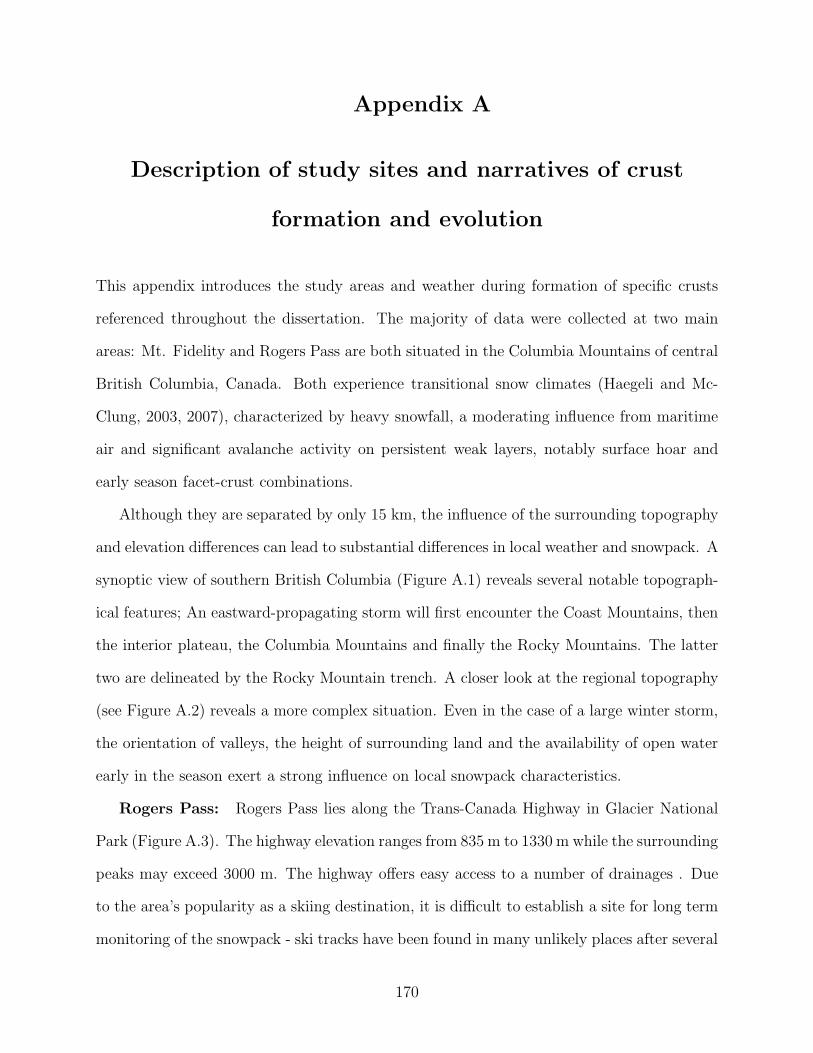
Appendix A
Description of study sites and narratives of crust
formation and evolution
This appendix introduces the study areas and weather during formation of specific crusts
referenced throughout the dissertation. The majority of data were collected at two main
areas: Mt. Fidelity and Rogers Pass are both situated in the Columbia Mountains of central
British Columbia, Canada. Both experience transitional snow climates (Haegeli and Mc-
Clung, 2003, 2007), characterized by heavy snowfall, a moderating influence from maritime
air and significant avalanche activity on persistent weak layers, notably surface hoar and
early season facet-crust combinations.
Although they are separated by only 15 km, the influence of the surrounding topography
and elevation differences can lead to substantial differences in local weather and snowpack. A
synoptic view of southern British Columbia (Figure A.1) reveals several notable topograph-
ical features; An eastward-propagating storm will first encounter the Coast Mountains, then
the interior plateau, the Columbia Mountains and finally the Rocky Mountains. The latter
two are delineated by the Rocky Mountain trench. A closer look at the regional topography
(see Figure A.2) reveals a more complex situation. Even in the case of a large winter storm,
the orientation of valleys, the height of surrounding land and the availability of open water
early in the season exert a strong influence on local snowpack characteristics.
Rogers Pass: Rogers Pass lies along the Trans-Canada Highway in Glacier National
Park (Figure A.3). The highway elevation ranges from 835 m to 1330 m while the surrounding
peaks may exceed 3000 m. The highway offers easy access to a number of drainages . Due
to the area’s popularity as a skiing destination, it is difficult to establish a site for long term
monitoring of the snowpack - ski tracks have been found in many unlikely places after several
170

Figure A.1: Mountains of Western British Columbia. Base image from Google Maps (Google,2013).
Figure A.2: Topography and location around study areas referenced in this dissertation. Dig-ital Elevation data from Geobase.ca (Natural Resources Canada, Earth Sciences Sector, Cen-tre for Topographic Information, 2013).
171

Table A.1: Study Sites in Rogers Pass. Abbreviations used in crust identifiers are in paren-theses.
Name Elev. Asp. Veg. NotesFidelity Study Plot (FI) 1905 m flat TL Met stnBeaver Valley (BV) 870 m flat BTL Old gravel pitRogers Pass Study Plot (RP) 1305 m flat BTL Met stnFidelity South Run (SR) 1950 m SE BTL Small open glade.RP Study Slope (RP) 1890 m ENE BTL Below Fidelity Met stn
hours of digging. For this reason all study sites were established either in areas closed to
recreational use or with no open slopes for skiing. Table A.1 summarizes the topography and
vegetation at each study site. Two sites, at the Mt. Fidelity and Rogers Pass study plots,
were adjacent to meteorological instrumentation. Both are equipped with precipitation and
temperature gauges while Fidelity is also equipped with long and shortwave radiometers.
Along with the Fidelity study plot, the South Run and Study Slope sites were situated in an
area closed to public access during the winter season. Figure A.4 shows the area surrounding
the Mt. Fidelity station. Fidelity study plot is known as a site with little to no wind effect
and a very uniform snowpack, making it ideal for tracking changes over time of specific
layers.
This remainder of this appendix summarizes the general characteristics of each crust
that was observed in the field along with crusts observed in the Rogers Pass cold lab. Each
crust is named according to general location and date of first burial. This is consistent with
the guidelines for naming persistent weak layers given in CAA (2007). Knowledge of the
weather leading up to the formation of the crust and its subsequent burial can be useful
for making inferences about the spatial variability and extent of a given crust; for instance
the winter of 2009-2010 was notable for the persistent ridges of high pressure over much of
interior British Columbia. Temperatures were mild and there was little precipitation. As a
result, crusts formed by the end of January on all unshaded south-facing slopes. Structure
and variability were dictated mostly by the slope and aspect as well as any shade provided
172
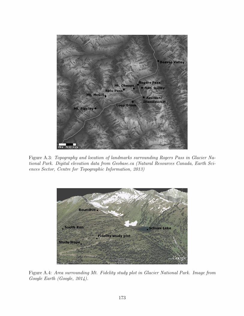
Figure A.3: Topography and location of landmarks surrounding Rogers Pass in Glacier Na-tional Park. Digital elevation data from Geobase.ca (Natural Resources Canada, Earth Sci-ences Sector, Centre for Topographic Information, 2013)
Figure A.4: Area surrounding Mt. Fidelity study plot in Glacier National Park. Image fromGoogle Earth (Google, 2014).
173

by local vegetation.
A.1 2007-08 Crust
FI071205: This crust formed as the result of a warm, moist air mass (‘Pineapple Express’)
that moved into British Columbia from the southwest in early December 2007. The system
brought elevated freezing levels and rain or wet snow up to 2000 m in the North Columbia
mountains. Cooler temperatures and snow followed throughout the next day and the crust
was buried. The ‘December 5th‘ crust exhibited a large degree of variability at all spatial
scales and included percolation channels, ice lenses and laminations. The crust was moni-
tored at a fixed study site on the Mt. Fidelity study slope from 2 January – 29 March 2008.
It was also observed and tested at a number of other sites in Glacier National Park, Blue
River and Kicking Horse Mountain Resort . This crust is discussed further in Smith et al.
(2008). This is one of only 2 crusts in the data set that formed as the result of precipitation;
all others were due to incoming solar radiation, elevated air temperature or a combination
of the two.
Figure A.5 shows the air temperature and liquid precipitation recorded at the Mt. Fidelity
weather station. The temperature rose to above freezing from 03:00 PST 4 December and
remained above freezing until 17:00. During this time 13 mm of precipitation fell, likely as a
mixture of wet snow and rain. The air temperature then fell over the next 48 hours, with an
additional 17 mm of precipitation falling as snow. This rapid transition from wet snow or rain
to cooler temperatures and snowfall allowed for an extended period of conditions suitable to
temperature gradient metamorphism within the wetted layer and at its boundaries as the
liquid water froze.
Clear cold conditions continued until 11 December (Figure A.6), when another period of
snowfall began and the crust was rapidly buried over 1 m deep in the snowpack. Weekly site
visits commenced 2 January, 2008 and thermistors were in place within the crust and at its
174

−20
−15
−10
−5
0
Mea
n H
ourly
Tem
pera
ture
[o C]
TMeanPCP1hr
12/0
3 12
:00
12/0
4 00
:00
12/0
4 12
:00
12/0
5 00
:00
12/0
5 12
:00
12/0
6 00
:00
12/0
6 12
:00
12/0
7 00
:00
12/0
7 12
:00
0
1
2
3
4
5
1hr
Pre
cipi
tatio
n [m
m]
Figure A.5: Hourly air temperature and precipitation at Mt. Fidelity weather station duringthe formation of crust CR071205.
175

−25
−20
−15
−10
−5
0
5M
ean
Dai
ly T
empe
ratu
re [o C
]TMeanPCP24
11/0
211
/16
11/3
012
/14
12/2
801
/11
01/2
502
/08
02/2
203
/07
03/2
10
5
10
15
20
25
30
35
40
45
50
24hr
Pre
cipi
tatio
n [m
m]
Figure A.6: Air temperature and daily precipitation at Mt. Fidelity weather station, winter2007-08
boundaries from 14 January - 25 February. The crust was observed weekly at a fixed study
plot at Mt. Fidelity and also at various sites and elevations in the Rogers Pass, Blue River
and Kicking Horse Mountain Resort areas until the conclusion of the study season in mid-
March. Standard observations at the fixed study plot included Propagation Saw Test (PST),
shear frame tests and a test profile.
A.2 2008-09 Crusts
Unlike the previous winter which had very few clear sunny periods after early December,
winter 2008-09 was marked by several clear sunny periods which allowed for the formation
of thick sun crusts on south-facing slopes. Three crusts were tracked this winter, all located
on the South Run area of the Mt. Fidelity closure. Figure A.7 shows the air temperature
and liquid precipitation recorded at the Mt. Fidelity weather station from early January
176

−25
−20
−15
−10
−5
0
5M
ean
Dai
ly T
empe
ratu
re [o C
]TMeanPCP24
01/1
701
/31
02/1
402
/28
03/1
403
/28
04/1
10
5
10
15
20
25
24hr
Pre
cipi
tatio
n [m
m]
Figure A.7: Air temperature and daily precipitation at Mt. Fidelity weather station, winter2008-09.
to early April 2009, while Figure A.8 shows the measured incoming solar and net longwave
radiation. Radiation data were lost for a 2-week period in late February when a datalogger
battery failed.
SR090127: This crust formed on south-facing slopes during a warm, sunny period in late
January. Maximum temperatures reached 8.0 ◦C on 20 January, followed by a cooling trend
through 27 January when the crust was buried. Thermistors were placed within the crust
and at its upper and lower boundaries at a fixed study site on Mt. Fidelity South Run on 18
January and site visits continued weekly until 11 April at which point the crust was still 71
cm below the surface. Standard observations included NIR, PST, shear frames at the upper
boundary and a test profile.
SR090222: The crust formed on south-facing slopes following a period of generally clear
weather. Unlike the conditions preceding the formation of SR090127, air temperatures did
not rise above 0 ◦C and melting of surface snow was due entirely to incoming solar radiation.
177

0
50
100
150
200
250
300
Inco
min
g S
hort
wav
e R
adia
tion
[W m
−2 ] 24hr trailing avg SW
Hourly LW
01/1
601
/30
02/1
302
/27
03/1
303
/27
04/1
0
−200
−150
−100
−50
0
50
Net
Lon
gwav
e R
adia
tion
[W m
−2 ]
Figure A.8: Incoming shortwave and net longwave radiation at Mt. Fidelity weather station,winter 2008-09. Data are missing from 20 February - 5 March due to the failure of thedatalogger battery.
178

The crust was buried late on 22 February and thermistors were placed within the crust and
at its boundaries on 24 February. Weekly site visits continued until 11 April and thermistors
were removed on 17 April. The crust was 50 cm below the surface at the time of the final
observation. Standard weekly observations were the same as for SR090127.
SR090301: A short period of clear sunny skies in late February was responsible for the
formation of this crust, which was quickly buried on 1 March and by the time of the first
study plot visit on 5 March was 20 cm below the snow surface. Thermocouples were placed
within and around the crust on 7 March. Weekly visits continued until 11 April and standard
observations were the same as for SR090127 and SR090222.
A.3 2009-10 Crusts
The winter of 2009-10 was generally very warm, with the mean daily temperature rarely
dropping below -7 ◦C at Mt. Fidelity weather station. The period from mid-January to
mid-March was marked with alternating periods of clear weather and light precipitation at
Mt. Fidelity and Rogers Pass, as shown in Figures A.9 and A.11, respectively. Incoming
shortwave radiation and net longwave radiation at Mt. Fidelity are shown in Figure A.10.
Periods of clear skies occurred when the net longwave is strongly negative and the amplitude
of the incoming shortwave radiation is larger, for instance around 12 February.
Natural crusts were formed at Mt. Fidelity by freezing rain, incoming solar radiation and
temperature. Rainfall and wet snow formed crusts at Rogers Pass and Beaver Valley but
did not extend as high as Mt. Fidelity. Natural crusts were also harvested at Rogers Pass
and studied in a cold lab. Thermal conductivity measurements were first used on crusts this
season.
Fidel100109: This 2 mm thick crust was formed by a freezing rain event at Mt Fidelity
on the evening of 9 January, 2010. Air Temperatures were well below 0 ◦C and the wetted
snow was buried by 2 cm of snow several hours later. Thermocouples were placed above
179
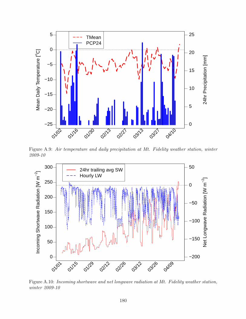
−25
−20
−15
−10
−5
0
5M
ean
Dai
ly T
empe
ratu
re [o C
]TMeanPCP24
01/0
201
/16
01/3
002
/13
02/2
703
/13
03/2
704
/10
0
5
10
15
20
25
24hr
Pre
cipi
tatio
n [m
m]
Figure A.9: Air temperature and daily precipitation at Mt. Fidelity weather station, winter2009-10
0
50
100
150
200
250
300
Inco
min
g S
hort
wav
e R
adia
tion
[W m
−2 ] 24hr trailing avg SW
Hourly LW
01/0
101
/15
01/2
902
/12
02/2
603
/12
03/2
604
/09
−200
−150
−100
−50
0
50
Net
Lon
gwav
e R
adia
tion
[W m
−2 ]
Figure A.10: Incoming shortwave and net longwave radiation at Mt. Fidelity weather station,winter 2009-10
180
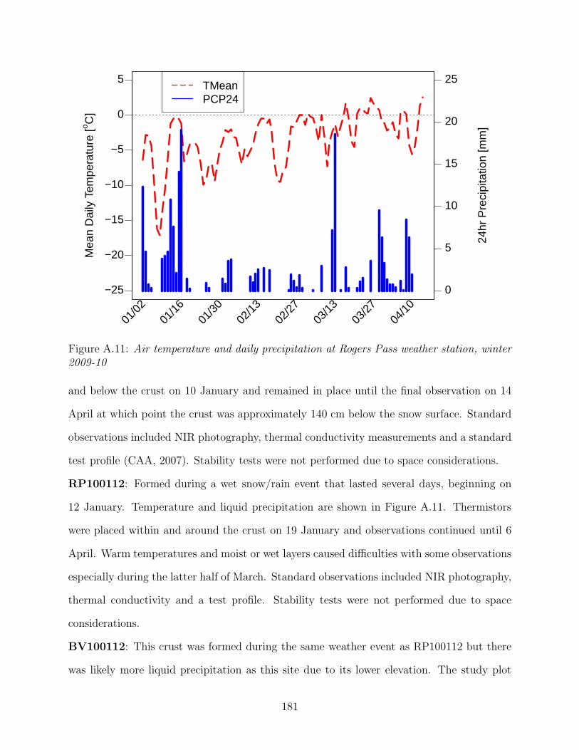
−25
−20
−15
−10
−5
0
5M
ean
Dai
ly T
empe
ratu
re [o C
]TMeanPCP24
01/0
201
/16
01/3
002
/13
02/2
703
/13
03/2
704
/10
0
5
10
15
20
25
24hr
Pre
cipi
tatio
n [m
m]
Figure A.11: Air temperature and daily precipitation at Rogers Pass weather station, winter2009-10
and below the crust on 10 January and remained in place until the final observation on 14
April at which point the crust was approximately 140 cm below the snow surface. Standard
observations included NIR photography, thermal conductivity measurements and a standard
test profile (CAA, 2007). Stability tests were not performed due to space considerations.
RP100112: Formed during a wet snow/rain event that lasted several days, beginning on
12 January. Temperature and liquid precipitation are shown in Figure A.11. Thermistors
were placed within and around the crust on 19 January and observations continued until 6
April. Warm temperatures and moist or wet layers caused difficulties with some observations
especially during the latter half of March. Standard observations included NIR photography,
thermal conductivity and a test profile. Stability tests were not performed due to space
considerations.
BV100112: This crust was formed during the same weather event as RP100112 but there
was likely more liquid precipitation as this site due to its lower elevation. The study plot
181
was established in an old gravel pit on 31 January and thermistors were placed above, below
and within the crust to record the hourly temperature. Weekly observations continued
until thermistors were removed on 27 March. As was the case with RP100112, persistent
warm temperatures caused difficulties with observations during some site visits. Standard
observations included NIR photography, thermal conductivity and a test profile.
SR100131,SR100210: These crusts formed on south-facing slopes in late January and
early February during consecutive clear, sunny periods. Ambient air temperature at Mt.
Fidelity, several hundred metres away at a similar elevation, averaged -5 ◦C during formation
of both crusts. The study site was on Mt. Fidelity South Run, within the public closure
area. Due to low snow and strong insolation during February and early March these two
crusts became one and tracking specific features became difficult due to continued melting
and percolation. Thermistors were placed in SR100131 on 3 February and in SR100210 on
10 February. Weekly observations continued until 7 April and included NIR photography,
thermal conductivity above, below and within, and a test profile. The upper snowpack
containing the crusts became isothermal in late March and remained so until the end of the
season.
FI100308: Formation occurred during a series of warm and sunny days with minimal pre-
cipitation in early March. The study site was on flat terrain in the Mt. Fidelity study plot
coincident with the study site for FI100109. The crust was first observed on 8 March and
weekly observations continued until 14 April at which point the crust was approximately 85
cm below the surface. Standard observations included NIR photography, thermal conduc-
tivity above, below and within the crust and a standard test profile. Stability tests were not
performed due to space considerations.
SR09site:A spatial variability study was performed on the SR100131 crust at the same site
used for the 2009 crusts. Observations were spaced along two grid lines running upslope and
included NIR photography, thermal conductivity and a test profile.
182

LAB: Crusts were harvested from an area adjacent to the Rogers Pass staff residence and
transported in an insulated box to the cold lab approximately 100 m distant. The natural
crust was formed by the same processes responsible for RP100112. Observations prior to
harvesting included NIR photography, thermal conductivity within the crust and in adjacent
layers, and a test profile. Five cold lab experiments were performed and conditions for each
are described in more detail in Chapters 2, 3 and 4.
183

Appendix B
Glossary
This appendix includes definitions of some commonly-used terms and acronyms. References
to further information are included where appropriate.
Bond: The region of ice lattice connecting two discrete snow particles.
Bridging: Refers to the ability of a stiff snow slab to reduce or spread the force transmitted
to a buried weak layer.
Compression Test (CT): A test for ease of initiation of a weak layer in the seasonal snow
pack. A layer of interest does not need to be identified beforehand. A column 30 cm x 30
cm is isolated to a depth of up to 1 – 1.5 m and increasing loading is applied to the top of
the column with a snow shovel. Interpretation is dependent on the number of ’taps’ on the
shovel required before the weak layer fails as well as the manner in which it fails. Described
by CAA (2007).
Coordination Number: The number of bonds per snow grain; influences heat transfer
and snowpack settling. Often an intrinsic property of layers in snowpack models.
Correlation Length: The distance beyond which variations of the dialectric constant in
one region of space become uncorrelated with those in another region (Toure et al., 2008).
In the context of the present study, the correlation length is proportional to optical grain
size and inversely proportional to SSA.
Disaggregated: In the context of a crust, refers to an area where bonds are extremely weak
or broken. When referring to crystal photography, the bonds are broken manually in order
to examine individual crystals.
Equilibrium Metamorphism (see also: Temperature Gradient Metamorphism): Snow
grain metamorphism that is driven by localized curvature-dependent gradients in vapour
184

pressure rather than a temperature gradient. The equilibrium vapour pressure is higher over
grains with a smaller radius of curvature, and such grains will tend to lose mass while grains
with a larger radius of curvature gain mass. Typically results in well-bonded snow comprised
of rounded grains.
Extended Column Test (ECT): A test of the ease of initiation and propagation propen-
sity of a weak layer, though the weak layer does not need to be identified beforehand.
Techniques and recording standards introduced by Simenhois and Birkeland (2007). Similar
to the Compression Test, except that the column is isolated 90 cm across the slope instead
of 30 cm.
Faceting: The metamorphism of snow grains from either fresh or rounded forms to forms
exhibiting sharp edges and flat faces. Usually associated with a slope-normal temperature
gradient greater than 1 ◦C 10 cm−1.
Grain size: Typically describes the average diameter, or sometimes size range, in a repre-
sentative sample of snow crystals. A somewhat fuzzy concept when attempting to quantify
physical characteristics if there is no clear delineation between grain and bond.
Grain Type: Grain type for seasonal snow is classified by considering both shape and
metamorphic pathway. Fierz et al. (2009) uses a system of major classes and subclasses
communicated as four-letter abbreviations. The major class is the first two letters and the
subclass, if used, is the following two lowercase letters. Major classes and subclasses used in
this dissertation are listed in Table B.1 alongside a previous system published by Colbeck
et al. (1992).
Hand Hardness: A hardness scale developed help field workers quickly determine the
relative hardness of snow layers. Values in order of increasing hardness are, “fist”,“four
fingers”,“one finger”,“pencil”,“knife” and “ice”, and are determined by which object can
penetrate the snow with moderate force.
185

Table B.1: Grain type abbreviations. The full classification systems have major classes andsubclasses. Only those subclasses used in the paper are included in the table. For a full listconsult the relevant publication.
Grain Type Fierz et al. (2009) Colbeck et al. (1992)Precipitation Particles PP 1Decomposing forms DF 2Rounded grains RG 3Rounded grains, faceting RGxf 3cRounded grains, wind packed RGwp 9dFaceted crystals FC 4Faceted crystals, rounding FCxr 4cDepth hoar DH 5bSurface hoar SH 7Melt freeze crust MFcr 9eClustered grains MFcl 6aRefrozen polycrystals MFpc 6bIce layer IF 8,9c
Micro-Computed Tomography (µCT): A non-destructive imaging technique used to
compute a physical model of an object, with resolution on the micron scale. In snow science
the technique has been used to study structure, bonds and metamorphism of small snow
samples in a lab.
Neck: Sometimes used to refer to bonds, so-called because of the constriction of the idealized
bond (example shown in Figure 1.2.).
Optical Diameter (snow): For a given portion of the visible or near-infrared range of
the electromagnetic spectrum, the diameter of a sphere (or collection of spheres) having the
same optical properties as a snow crystal, or collection of crystals. Inversely proportional to
the Specific Surface Area in the near-infrared range, and sometimes treated as an intrinsic
property of snow in snowpack models.
Overburden: Refers to the column snow water equivalent overlying a particular layer within
the snowpack. May be measured exactly by using a cylindrical tube of known diameter and
extracting, then weighing a continuous core from the snow surface down to the layer, or may
186

be estimated from densities collected from a full or test snow profile.
Pore Intercept Length: A term used in stereological modeling to denote the ratio of
element volume to area. The inverse of specific surface area.
Persistent Weak Layer: Sometimes abbreviated as PWL, describes a weak layer in the
snowpack that persists for several weeks or months. These layers often go ’dormant’ and
become difficult to trigger for extended periods before suddenly becoming reactive dynamic
loading from skiers, snowmobilers or cornices,
Propagation Saw Test (PST): A test of the propagation propensity of a layer in the
seasonal snow pack, usually a persistent weak layer which must be identified beforehand.
Formalized by Gauthier and Jamieson (2008) and studied further by a number of authors
including Ross (2010). A column is 30 cm wide and either 90 cm or the depth of the weak
layer, whichever is greater, is isolated. The blunt edge of a snow saw is run through the weak
layer, starting from the downslope end of the column. Cutting is stopped once the fracture
propagates ahead of the saw. Interpretation of the propagation propensity is based on the
ratio of the cut length to the overall column length.
Radius of Curvature: Radius of a sphere that is (usually) used to approximate the shape
and size of a grain of snow. Principally important due to the fact that equilibrium vapour
pressure over ice increases as the radius of curvature decreases.
Rayleigh Number (critical): A dimensionless number used to describe the relative im-
portance of convection and conduction in a fluid. The critical Rayleigh Number is the point
at which convection dominates conduction.
Slab: A region of relatively stiff, supportable snow overlying a weak layer. Slab thickness,
density and stiffness contribute to the propagation of failures in buried weak layers in the
snowpack but may also bridge weak layers.
Scale: The physical distance over which phenomena are measured or over which natural pro-
cesses act. Bloschl and Sivapalan (1995) defined a ‘scale triplet’ which define measurements
187

taken over a given scale. These include the spacing, the extent and the support. Schweizer
et al. (2008) summarize the scale and scale triplets as they apply to snow avalanche studies.
Specific Surface Area: The ratio of an element’s surface area to volume. Can be used as a
proxy for observing structural changes in an aggregate of snow crystals. Typically the specific
surface area will be large for new snow crystals with dendritic shapes, and will decrease with
mechanical compaction and equilibrium metamorphism, or rounding. Inversely proportional
to the optical diameter.
Temperature Gradient Metamorphism: (see also: Equilibrium Metamorphism): Snow
metamorphism that is driven by a gradient in temperature, resulting in a gradient in water
vapour. Growth trends toward edged crystals with flat faces (’facets’) and this process tends
to produce a weaker, poorly-bonded snowpack.
Thermal Diffusivity: The ratio of the thermal conductivity to the product of density and
specific heat capacity. In Fourier analysis of thermal conductivity the thermal diffusivity is
measured directly and the thermal conductivity is derived from the measurement.
(Effective) Thermal Conductivity (keff) : The ability of a material to conduct heat.
In modeling studies this is often broken down into separate terms representing the thermal
conductivity due to sensible and latent heat transfer through the material. In field studies
it is often impractical or impossible to distinguish between the two and thus a total effective
conductivity is used. The terms thermal conductivity, bulk thermal conductivity and effective
thermal conductivity are used interchangeably throughout this text.
Tortuosity: Defined by Kaempfer et al. (2005) as ‘the square of the ratio of the effective
path of diffusion through a porous medium to the length along the major diffusion axis’.
The tortuosity may be used to describe how water vapour diffuses through the pore space
within the snowpack. Samples with high values of tortuosity will tend toward lower values
(and thus more direct thermal pathways) under an induced thermal temperature gradient.
188

Appendix C
Thermal Conductivity and Layer Characteristics
Table C.1: Layer characteristics for 2008-09 crusts. La-
bels and units: Temperature (T,[◦C]); Grain Type (F);
Layer Resistance (R); Density (ρ,[kg m−3]); Layer Mois-
ture (θ).
Crust Date T F R ρ θ
SR0127 09/02/02 -7.5 MFcr K- 282 D
SR0127 09/02/10 -5.3 MFcr K- 276 D
SR0127 09/02/21 -4.6 MFcr K- 290 D
SR0127 09/03/05 -1.3 MFcr K 280 D
SR0127 09/03/12 -3.5 MFcr K 266 D
SR0127 09/03/21 -2.6 MFcr* K* 300 D
SR0127 09/03/27 -1.0 MFcr* P+* 318 D
SR0127 09/04/06 -0.3 MFpc 1F+ 335 M
SR0127 09/04/11 0.0 MFpc* P-* 313 M
SR0222 09/02/24 -2.5 Mfcr K 290 D
SR0222 09/03/05 -1.8 Mfcr K 331 D
SR0222 09/03/12 -5.3 Mfcr K 290 D
SR0222 09/03/21 -3.0 Mfcr K- 290 D
SR0222 09/03/27 -0.9 Mfcr K- 311 D
SR0222 09/04/06 0.1 Mfcr* P+* 306 M
X: Not recorded. *: Variable
189
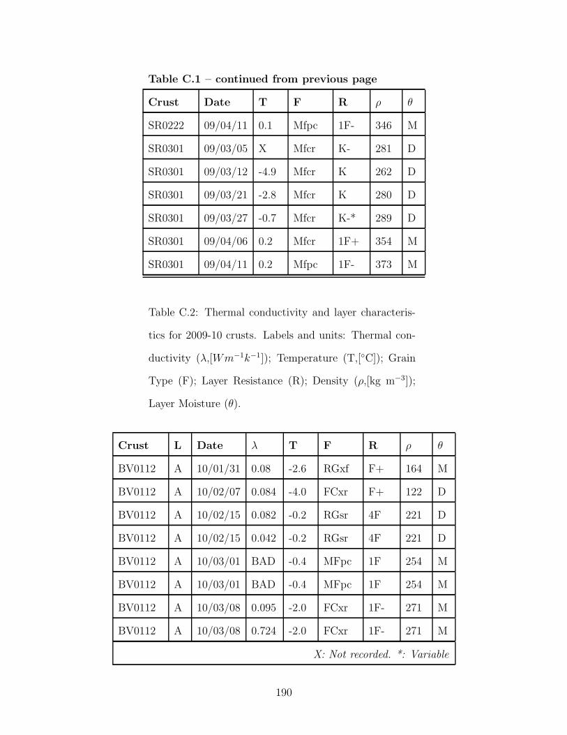
Table C.1 – continued from previous page
Crust Date T F R ρ θ
SR0222 09/04/11 0.1 Mfpc 1F- 346 M
SR0301 09/03/05 X Mfcr K- 281 D
SR0301 09/03/12 -4.9 Mfcr K 262 D
SR0301 09/03/21 -2.8 Mfcr K 280 D
SR0301 09/03/27 -0.7 Mfcr K-* 289 D
SR0301 09/04/06 0.2 Mfcr 1F+ 354 M
SR0301 09/04/11 0.2 Mfpc 1F- 373 M
Table C.2: Thermal conductivity and layer characteris-
tics for 2009-10 crusts. Labels and units: Thermal con-
ductivity (λ,[Wm−1k−1]); Temperature (T,[◦C]); Grain
Type (F); Layer Resistance (R); Density (ρ,[kg m−3]);
Layer Moisture (θ).
Crust L Date λ T F R ρ θ
BV0112 A 10/01/31 0.08 -2.6 RGxf F+ 164 M
BV0112 A 10/02/07 0.084 -4.0 FCxr F+ 122 D
BV0112 A 10/02/15 0.082 -0.2 RGsr 4F 221 D
BV0112 A 10/02/15 0.042 -0.2 RGsr 4F 221 D
BV0112 A 10/03/01 BAD -0.4 MFpc 1F 254 M
BV0112 A 10/03/01 BAD -0.4 MFpc 1F 254 M
BV0112 A 10/03/08 0.095 -2.0 FCxr 1F- 271 M
BV0112 A 10/03/08 0.724 -2.0 FCxr 1F- 271 M
X: Not recorded. *: Variable
190

Table C.2 – continued from previous page
Crust L Date λ T F R ρ θ
BV0112 A 10/03/14 BAD -2.7 FCso 1F- 229 M
BV0112 A 10/03/14 0.077 -2.7 FCso 1F- 229 M
BV0112 A 10/03/23 BAD 0.0 MFcr P+ 392 M
BV0112 A 10/03/23 0.056 0.0 MFcr P+ 392 M
BV0112 B 10/01/31 0.100 -3.1 FCxr 4F 257 M
BV0112 B 10/01/31 0.145 -3.1 FCxr 4F 257 M
BV0112 B 10/01/31 0.104 -3.1 FCxr 4F 257 M
BV0112 B 10/02/07 BAD -3.5 Fcso 1F 249 D
BV0112 B 10/02/15 BAD -0.4 MFpc 4F+ 278 D
BV0112 B 10/02/15 0.058 -0.4 MFpc 4F+ 278 D
BV0112 B 10/03/01 0.052 -0.6 MFCL P- 311 M
BV0112 B 10/03/01 BAD -0.6 MFCL P- 311 M
BV0112 B 10/03/08 0.319 -3.0 FCxr 1F+ 278 M
BV0112 B 10/03/08 0.189 -3.0 FCxr 1F+ 278 M
BV0112 B 10/03/14 0.254 -1.4 FCxr 4F+ 277 M
BV0112 B 10/03/14 BAD -1.4 FCxr 4F+ 277 M
BV0112 B 10/03/23 BAD -0.1 MFpc 4F+ 343 M
BV0112 B 10/03/23 BAD -0.1 MFpc 4F+ 343 M
BV0112 I 10/01/31 0.150 -2.9 MFcr P+ 321 D
BV0112 I 10/01/31 0.193 -2.9 MFcr P+ 321 D
BV0112 I 10/02/07 BAD -3.9 MFcr P- 306 D
BV0112 I 10/02/15 0.209 -0.3 MFpc 1F 335 D
X: Not recorded. *: Variable
191

Table C.2 – continued from previous page
Crust L Date λ T F R ρ θ
BV0112 I 10/02/15 0.079 -0.3 MFpc 1F 335 D
BV0112 I 10/03/01 BAD -0.7 MFcl P-* 298 M
BV0112 I 10/03/01 BAD -0.7 MFcl P-* 298 M
BV0112 I 10/03/08 0.062 -2.6 MF P 272 D
BV0112 I 10/03/08 0.135 -2.6 MF P 272 D
BV0112 I 10/03/14 BAD -2.2 MFpc P-* 223 M
BV0112 I 10/03/14 BAD -2.2 MFpc P-* 223 M
BV0112 I 10/03/14 0.206 -2.2 MFpc P-* 223 M
BV0112 I 10/03/14 0.317 -2.2 MFpc P-* 223 M
BV0112 I 10/03/23 BAD 0.0 MFcr 4F 367 M
BV0112 I 10/03/23 BAD 0.0 MFcr 4F 367 M
BV0112 V 10/03/08 5.136 0.0 X D
BV0112 V 10/03/14 0.279 0.0 X M
BV0112 V 10/03/23 BAD 0.0 X X M
FI0110 A 10/01/10 0.108 -4.1 PPrm F 97 D
FI0110 A 10/01/10 BAD -4.1 PPrm F 97 D
FI0110 A 12/01/10 0.118 -3.0 MF 4F+ 136 M
FI0110 A 18/01/10 0.139 -3.6 FCxr 1F 226 D
FI0110 A 18/01/10 0.147 -3.6 FCxr 1F 226 D
FI0110 A 25/01/10 0.140 -4.7 RGsr P- 244 D
FI0110 A 25/01/10 0.160 -4.7 RGsr P- 244 D
FI0110 A 25/01/10 0.175 -4.7 RGsr P- 244 D
X: Not recorded. *: Variable
192

Table C.2 – continued from previous page
Crust L Date λ T F R ρ θ
FI0110 A 02/02/10 0.161 -4.1 FCxr 1F+ 236 D
FI0110 A 02/02/10 0.156 -4.1 FCxr 1F+ 236 D
FI0110 A 02/02/10 0.201 -4.1 FCxr 1F+ 236 D
FI0110 A 08/02/10 0.179 -3.9 FCxr 1F+ 284 D
FI0110 A 08/02/10 0.205 -3.9 FCxr 1F+ 284 D
FI0110 A 17/02/10 0.176 -3.0 FCxr P- 287 D
FI0110 A 17/02/10 0.213 -3.0 FCxr P- 287 D
FI0110 A 28/02/10 0.208 -3.2 FCxr P+ 347 D
FI0110 A 28/02/10 0.201 -3.2 FCxr P+ 347 D
FI0110 A 09/03/10 0.192 -2.3 RGlr P 345 D
FI0110 A 09/03/10 0.292 -2.3 RGlr P 345 D
FI0110 A 15/03/10 0.212 -2.4 RGsr P- 346 M
FI0110 A 15/03/10 0.236 -2.4 RGsr P- 346 M
FI0110 A 10/03/22 0.222 -2.0 FCxr P+ 341 D
FI0110 A 10/03/22 0.261 -2.0 FCxr P+ 341 D
FI0110 A 10/03/28 BAD -1.6 RGsr P+ 372 M
FI0110 A 10/03/28 0.356 -1.6 RGsr P+ 372 M
FI0110 A 10/04/07 0.354 -1.6 FCxr P+ 378 D
FI0110 A 10/04/14 0.320 -1.6 FCxr K- 397 D
FI0110 A 10/04/14 BAD -1.6 FCxr K- 397 D
FI0110 B 10/01/10 0.046 -4.6 PP F+ 112 D
FI0110 B 10/01/10 0.040 -4.6 PP F+ 112 D
X: Not recorded. *: Variable
193

Table C.2 – continued from previous page
Crust L Date λ T F R ρ θ
FI0110 B 12/01/10 0.089 -2.9 FCxr 4F- 139 D
FI0110 B 12/01/10 0.096 -2.9 FCxr 4F- 139 D
FI0110 B 18/01/10 0.157 -3.6 FCxr 1F 223 D
FI0110 B 18/01/10 0.104 -3.6 FCxr 1F 223 D
FI0110 B 25/01/10 0.131 -4.8 FCxr 1F 248 D
FI0110 B 25/01/10 0.129 -4.8 FCxr 1F 248 D
FI0110 B 02/02/10 0.168 -4.2 FCxr P- 269 D
FI0110 B 02/02/10 0.162 -4.2 FCxr P- 269 D
FI0110 B 02/02/10 0.161 -4.2 FCxr P- 269 D
FI0110 B 02/02/10 0.134 -4.2 FCxr P- 269 D
FI0110 B 08/02/10 0.166 -3.9 FCxr 1F- 297 D
FI0110 B 08/02/10 0.170 -3.9 FCxr 1F- 297 D
FI0110 B 17/02/10 0.148 -3.1 RGsr P 323 D
FI0110 B 17/02/10 0.215 -3.1 RGsr P 323 D
FI0110 B 28/02/10 0.200 -3.3 FCxr P+ 364 D
FI0110 B 28/02/10 BAD -3.3 FCxr P+ 364 D
FI0110 B 09/03/10 0.275 -2.3 FCxr P+ 375 D
FI0110 B 09/03/10 0.206 -2.3 FCxr P+ 375 D
FI0110 B 15/03/10 0.216 -2.5 RGsr P 382 M
FI0110 B 15/03/10 0.221 -2.5 RGsr P 382 M
FI0110 B 10/03/22 0.296 -2.0 FCxr K- 356 D
FI0110 B 10/03/28 0.553 -1.6 RGsr P+ 393 M
X: Not recorded. *: Variable
194

Table C.2 – continued from previous page
Crust L Date λ T F R ρ θ
FI0110 B 10/03/28 0.489 -1.6 RGsr P+ 393 M
FI0110 B 10/04/07 0.428 -1.2 FCxr K- 406 D
FI0110 B 10/04/14 0.467 -1.1 FCxr K- 430 D
FI0110 B 10/04/14 0.275 -1.1 FCxr K- 430 D
FI0110 I 08/02/10 0.188 -3.9 MFpc 1F+ X D
FI0110 I 17/02/10 0.219 -3.1 MFpc P X D
FI0110 I 28/02/10 0.175 -3.3 IFrc P X D
FI0110 I 28/02/10 0.209 -3.3 IFrc P X D
FI0110 I 09/03/10 0.265 -2.3 IFil K- X D
FI0110 I 09/03/10 BAD -2.3 IFil K- X D
FI0110 I 15/03/10 0.221 -2.5 IFrc M X M
FI0110 I 15/03/10 0.282 -2.5 IFrc M X M
FI0110 I 10/03/22 0.279 -2.0 IFrc K- X D
FI0110 I 10/03/22 0.258 -2.0 IFrc K- X D
FI0110 I 10/03/28 BAD -1.6 IFil P+ X M
FI0110 I 10/03/28 0.843 -1.6 IFil P+ X M
FI0110 I 10/04/07 0.220 -1.2 IFrc P+ X D
FI0110 I 10/04/14 BAD -1.1 IFrc K- X D
FI0110 I 10/04/14 0.421 -1.1 IFrc K- X D
FI0308 A 10/03/15 0.106 -3.7 Mfpc 4F 185 M
FI0308 A 10/03/15 0.074 -3.7 Mfpc 4F 185 M
FI0308 A 10/03/22 0.115 -2.9 DFdc 1F 166 M
X: Not recorded. *: Variable
195

Table C.2 – continued from previous page
Crust L Date λ T F R ρ θ
FI0308 A 10/03/22 0.122 -2.9 DFdc 1F 166 M
FI0308 A 10/03/28 0.130 -1.8 MFcl 1F+ 264 M
FI0308 A 10/03/28 0.166 -1.8 MFcl 1F+ 264 M
FI0308 A 10/04/07 0.203 -2.5 RGsr P 285 D
FI0308 A 10/04/14 0.262 -2.3 RGsr P+ 310 D
FI0308 A 10/04/14 0.290 -2.3 RGsr P+ 310 D
FI0308 B 10/03/15 0.088 -3.7 FCxr 4F+ 228 M
FI0308 B 10/03/15 0.098 -3.7 FCxr 4F+ 228 M
FI0308 B 10/03/22 0.143 -2.9 RGlr P- 252 D
FI0308 B 10/03/22 0.163 -2.9 RGlr P- 252 D
FI0308 B 10/03/28 0.158 -1.8 RGsr 1F 265 M
FI0308 B 10/03/28 BAD -1.8 RGsr 1F 265 M
FI0308 B 10/04/07 0.243 -2.3 RGsr P- 309 D
FI0308 B 10/04/14 0.301 -2.1 FCxr P+ 332 D
FI0308 B 10/04/14 0.256 -2.1 FCxr P+ 332 D
FI0308 I 10/03/15 0.055 -3.8 MFcr P X M
FI0308 I 10/03/15 0.239 -3.8 MFcr P X M
FI0308 I 10/03/22 0.183 -2.9 MFcr P+ X D
FI0308 I 10/03/22 0.204 -2.9 MFcr P+ X D
FI0308 I 10/03/28 0.186 -1.8 MFcr 1F 288 M
FI0308 I 10/03/28 2.103 -1.8 MFcr 1F 288 M
FI0308 I 10/04/07 0.178 -2.4 MFcr P- X D
X: Not recorded. *: Variable
196

Table C.2 – continued from previous page
Crust L Date λ T F R ρ θ
FI0308 I 10/04/14 0.133 -2.3 MFcr K X D
FI0308 I 10/04/14 0.218 -2.3 MFcr K X D
FI0308 V 10/03/15 0.102 -3.8 MFcr P X M
FI0308 V 10/03/22 0.170 -2.9 MFcr P+ X D
FI0308 V 10/03/28 0.290 -1.8 MFcr 1F 288 M
FI0308 V 10/03/28 0.173 -1.8 MFcr 1F 288 M
FI0308 V 10/04/07 0.180 -2.4 MFcr P- X D
FI0308 V 10/04/14 0.233 -2.3 MFcr K X D
FI0308 V 10/04/14 0.540 -2.3 MFcr K X D
RP0112 A 10/01/19 0.100 -2.7 DFdc 4F 162 D
RP0112 A 10/01/25 0.137 -5.8 FCxr 4F 207 D
RP0112 A 10/02/02 0.144 -2.7 RGlr 1F- 260 D
RP0112 A 10/02/02 0.123 -2.7 RGlr 1F- 260 D
RP0112 A 10/02/09 0.129 -3.7 FCxr 1F- 277 D
RP0112 A 10/02/09 0.112 -3.7 FCxr 1F- 277 D
RP0112 A 10/02/15 0.118 -2.8 FCxr 1F+ 273 D
RP0112 A 10/02/15 0.169 -2.8 FCxr 1F+ 273 D
RP0112 A 10/02/27 0.199 -2.2 FCxr 1F+ 277 M
RP0112 A 10/02/27 0.172 -2.2 FCxr 1F+ 277 M
RP0112 A 10/03/08 0.164 -3.9 FCxr 1F+ 300 D
RP0112 A 10/03/08 0.195 -3.9 FCxr 1F+ 300 D
RP0112 A 10/03/14 0.193 -2.3 FCxr 1F+ 327 M
X: Not recorded. *: Variable
197

Table C.2 – continued from previous page
Crust L Date λ T F R ρ θ
RP0112 A 10/03/14 0.174 -2.3 FCxr 1F+ 327 M
RP0112 A 10/03/23 0.330 0.0 MFcr P+ 392 M
RP0112 A 10/03/23 0.203 0.0 MFcr P+ 392 M
RP0112 A 10/03/29 1.107 -0.3 FCxr 1F 317 M
RP0112 A 10/03/29 2.411 -0.3 FCxr 1F 317 M
RP0112 A 10/03/29 BAD -0.3 FCxr 1F 317 M
RP0112 A 10/03/29 BAD -0.3 FCxr 1F 317 M
RP0112 A 10/03/29 BAD -0.3 FCxr 1F 317 M
RP0112 A 10/04/06 BAD -0.3 FCxr P- 314 M
RP0112 A 10/04/06 BAD -0.3 FCxr P- 314 M
RP0112 A 10/04/13 0.267 -0.4 FCxr 1F+ 332 M
RP0112 B 10/01/19 0.110 -1.6 FCxr 1F X D
RP0112 B 10/01/25 0.154 -3.5 FCxr P- 260 D
RP0112 B 10/02/02 0.160 -2.5 FCxr P- 301 D
RP0112 B 10/02/02 0.158 -2.5 FCxr P- 301 D
RP0112 B 10/02/09 0.140 -3.0 FCxr 1F 306 D
RP0112 B 10/02/09 0.125 -3.0 FCxr 1F 306 D
RP0112 B 10/02/27 0.194 -2.2 FCxr P+ 383 M
RP0112 B 10/02/27 0.196 -2.2 FCxr P+ 383 M
RP0112 B 10/03/08 0.269 -3.1 FCxr P 354 D
RP0112 B 10/03/08 0.228 -3.1 FCxr P 354 D
RP0112 B 10/03/08 0.173 -3.1 FCxr P 354 D
X: Not recorded. *: Variable
198

Table C.2 – continued from previous page
Crust L Date λ T F R ρ θ
RP0112 B 10/03/08 0.147 -3.1 FCxr P 354 D
RP0112 B 10/03/14 0.192 -2.1 FCXR P 371 M
RP0112 B 10/03/14 0.196 -2.1 FCXR P 371 M
RP0112 B 10/03/23 0.359 -0.1 MFpc 4F+ 343 M
RP0112 B 10/03/23 0.408 -0.1 MFpc 4F+ 343 M
RP0112 B 10/03/29 BAD -0.3 FC P+ 396 M
RP0112 B 10/03/29 BAD -0.3 FC P+ 396 M
RP0112 B 10/03/29 BAD -0.3 FC P+ 396 M
RP0112 B 10/04/06 BAD -0.3 FCso P+ 389 M
RP0112 B 10/04/06 BAD -0.3 FCso P+ 389 M
RP0112 B 10/04/13 BAD -0.3 FCxr P+ 407 M
RP0112 I 10/01/19 0.087 -2.0 MFcr* P* 190 D
RP0112 I 10/01/19 0.064 -2.0 MFcr* P* 190 D
RP0112 I 10/01/19 0.154 -2.0 MFcr* P* 190 D
RP0112 I 10/01/19 0.236 -2.0 MFcr* P* 190 D
RP0112 I 10/01/25 0.106 -4.8 MFcr* P* 220 D
RP0112 I 10/01/25 0.156 -4.8 MFcr* P* 220 D
RP0112 I 10/02/02 0.124 -2.3 MFcr* P* 222 D
RP0112 I 10/02/02 0.135 -2.3 MFcr* P* 222 D
RP0112 I 10/02/09 0.098 -3.3 MFpc 1F+* 229 D
RP0112 I 10/02/09 0.124 -3.3 MFpc 1F+* 229 D
RP0112 I 10/02/09 0.058 -3.3 MFpc 1F+* 229 D
X: Not recorded. *: Variable
199

Table C.2 – continued from previous page
Crust L Date λ T F R ρ θ
RP0112 I 10/02/15 0.220 -2.8 MFpc P+ 316 D
RP0112 I 10/02/15 0.239 -2.8 MFpc P+ 316 D
RP0112 I 10/02/27 0.180 -2.3 MFcr* P+* 313 M
RP0112 I 10/02/27 0.076 -2.3 MFcr* P+* 313 M
RP0112 I 10/03/08 0.109 -3.5 MFcr P* 331 D
RP0112 I 10/03/08 0.142 -3.5 MFcr P* 331 D
RP0112 I 10/03/14 0.179 -2.2 FCxr 4F+ 332 M
RP0112 I 10/03/14 0.139 -2.2 FCxr 4F+ 332 M
RP0112 I 10/03/23 BAD -0.1 MFcr 4F 367 M
RP0112 I 10/03/23 0.079 -0.1 MFcr 4F 367 M
RP0112 I 10/03/29 BAD -0.3 MFpc* 1F 343 M
RP0112 I 10/03/29 BAD -0.3 MFpc* 1F 343 M
RP0112 I 10/04/06 BAD -0.3 FC 1F+ 344 M
RP0112 I 10/04/06 BAD -0.3 FC 1F+ 344 M
RP0112 I 10/04/13 BAD -0.4 MFpc 1F- 318 M
RP0112 V 10/03/08 0.124 -3.5 MFcr P+* 331 D
RP0112 V 10/03/08 0.117 -3.5 MFcr P+* 331 D
RP0112 V 10/03/14 0.180 -2.2 FCxr 4F+ 332 M
RP0112 V 10/03/14 0.213 -2.2 FCxr 4F+ 332 M
RP0112 V 10/03/23 BAD -0.1 MFcr 4F 367 M
RP0112 V 10/03/23 0.204 -0.1 MFcr 4F 367 M
RP0112 V 10/03/29 BAD -0.3 MFpc* 1F 343 M
X: Not recorded. *: Variable
200

Table C.2 – continued from previous page
Crust L Date λ T F R ρ θ
RP0112 V 10/04/06 BAD -0.3 FC 1F+ 344 M
RP0112 V 10/04/06 BAD -0.3 FC 1F+ 344 M
RP0112 V 10/04/13 BAD -0.4 MFpc 1F- 318 M
LAB0312 I 13 12:00 BAD 0.0 X X X W
LAB0312 I 13 12:37 0.089 -0.5 I K M W
LAB0312 I 13 12:51 0.141 -0.5 I K M W
LAB0312 I 13 13:26 0.648 -2.9 I K M W
LAB0312 I 13 14:05 0.276 -0.5 I K M M
LAB0312 I 13 15:10 0.142 0.0 I K M D
LAB0330 A 30 09:30 BAD -0.2 MFpc K X M
LAB0330 B 30 09:30 BAD -0.2 MFpc K X M
LAB0330 I 30 09:30 BAD -0.2 MFpc K X M
LAB0330 I 30 09:30 BAD -0.2 MFpc K X M
LAB0330 V 30 09:30 0.094 -0.2 MFpc K X M
LAB0330 V 30 10:30 0.034 -0.2 MFpc K X M
LAB0330 V 30 10:30 0.065 -0.2 MFpc K X M
LAB0330 V 30 12:20 0.285 -0.5 MFpc K X M
LAB0330 V 30 12:20 BAD -0.5 MFpc K X M
LAB0330 V 30 14:12 0.249 -0.6 MFpc X X M
LAB0330 V 30 14:12 BAD -0.6 MFpc X X M
LAB0330 V 30 16:55 0.122 -0.6 MFpc K X M
LAB0330 V 30 16:55 0.193 -0.6 MFpc K X M
X: Not recorded. *: Variable
201

Table C.2 – continued from previous page
Crust L Date λ T F R ρ θ
LAB0330 V 30 21:50 0.236 -1.5 MFpc K X D
LAB0330 V 30 21:50 0.250 -1.5 MFpc K X D
LAB0330 V 31 07:25 0.000 0.0 MFpc K X D
LAB0330 V 31 07:25 0.000 0.0 MFpc K X D
LAB0409 V 09 13:00 BAD -0.2 MFpc X X M
LAB0409 V 09 13:00 0.072 -0.2 MFpc X X M
LAB0409 V 09 19:35 BAD -0.2 MFpc X X M
LAB0409 V 09 19:35 0.690 -0.2 MFpc X X M
LAB0409 V 10 01:15 0.136 -1.5 MFpc X X D
LAB0409 V 10 01:15 0.252 -1.5 MFpc X X D
LAB0409 V 10 08:20 0.130 -7.8 MFpc X X D
LAB0409 V 10 08:20 0.286 -7.8 MFpc X X D
LAB0409 V 10 14:30 0.270 -13.0 MFpc X X D
LAB0410 V 10 19:15 0.058 -0.1 MFpc X X M
LAB0410 V 10 19:15 0.025 -0.1 MFpc X X M
LAB0410 V 11 09:30 0.081 -7.0 MFpc X X D
LAB0410 V 11 09:30 0.178 -7.0 MFpc X X D
LAB0410 V 11 21:00 0.277 -12.5 MFpc X X D
LAB0410 V 11 21:00 0.302 -12.5 MFpc X X D
LAB0410 V 12 09:40 BAD -14.4 MFpc X X D
LAB0410 V 12 09:40 0.269 -14.4 MFpc X X D
LAB0410 V 12 21:05 0.225 -14.9 MFpc X X D
X: Not recorded. *: Variable
202

Table C.2 – continued from previous page
Crust L Date λ T F R ρ θ
LAB0410 V 12 21:05 0.246 -14.9 MFpc X X D
LAB0410 V 13 09:35 0.273 -14.1 MFpc X X D
LAB0410 V 13 09:35 0.409 -14.1 MFpc X X D
LAB0413 V 10/04/13 0.080 -1.5 MFpc 1f+ 400 M
LAB0413 V 10/04/13 BAD -1.5 MFpc 1f+ 400 M
LAB0413 V 10/04/14 BAD -2.6 MFpc K X D
LAB0413 V 10/04/14 0.293 -2.6 MFpc K X D
LAB0413 V 10/04/15 0.414 -6.0 MFpc K X D
LAB0413 V 10/04/15 0.330 -6.0 MFpc K X D
LAB0413 V 10/04/16 0.253 -8.4 MFpc K X D
LAB0413 V 10/04/16 0.302 -8.4 MFpc K X D
LAB0413 V 10/04/17 0.144 -8.7 MFpc K X D
LAB0413 V 10/04/17 0.248 -8.7 MFpc K X D
LAB0413 V 10/04/18 0.136 -8.6 MFpc K X D
LAB0413 V 10/04/18 0.241 -8.6 MFpc K X D
SR0131 A 10/02/03 0.080 -3.5 PP F 63 D
SR0131 A 10/02/03 0.065 -3.5 PP F 63 D
SR0131 A 10/02/10 0.044 -4.5 FCxr 4F 251 D
SR0131 A 10/02/10 0.096 -4.5 FCxr 4F 251 D
SR0131 A 10/02/17 0.099 -2.4 FCxr F 191 D
SR0131 A 10/02/17 0.096 -2.4 FCxr F 191 D
SR0131 A 10/03/02 BAD 0.0 X X X X
X: Not recorded. *: Variable
203

Table C.2 – continued from previous page
Crust L Date λ T F R ρ θ
SR0131 A 10/03/02 BAD 0.0 X X X X
SR0131 A 10/03/09 BAD 0.0 X X X X
SR0131 A 10/03/09 BAD 0.0 X X X X
SR0131 A 10/03/22 BAD 0.0 X X X X
SR0131 A 10/03/22 BAD -0.2 MFpc P- 318 M
SR0131 A 10/03/28 BAD 0.0 X X X M
SR0131 A 10/04/07 BAD 0.0 X X X M
SR0131 B 10/02/03 0.149 -3.8 FCxr 1F 168 D
SR0131 B 10/02/03 0.142 -3.8 FCxr 1F 168 D
SR0131 B 10/02/10 0.073 -4.0 FCxr 4F+ 240 D
SR0131 B 10/02/10 0.080 -4.0 FCxr 4F+ 240 D
SR0131 B 10/02/17 0.165 -2.3 FCXR 4F+ 272 D
SR0131 B 10/02/17 0.131 -2.3 FCXR 4F+ 272 D
SR0131 B 10/03/02 3.640 0.0 FCxr P- 295 M
SR0131 B 10/03/02 1.727 0.0 FCxr P- 295 M
SR0131 B 10/03/09 BAD 0.0 X X X W
SR0131 B 10/03/09 BAD 0.0 X X X W
SR0131 B 10/03/22 BAD 0.0 X X X W
SR0131 B 10/03/22 BAD 0.0 X X X W
SR0131 B 10/03/28 BAD 0.0 X X X M
SR0131 B 10/04/07 BAD 0.0 X X X W
SR0131 I 10/02/03 0.714 -3.4 MFcr K- 238 D
X: Not recorded. *: Variable
204
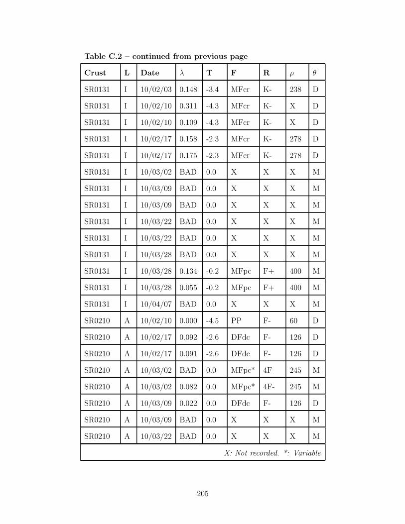
Table C.2 – continued from previous page
Crust L Date λ T F R ρ θ
SR0131 I 10/02/03 0.148 -3.4 MFcr K- 238 D
SR0131 I 10/02/10 0.311 -4.3 MFcr K- X D
SR0131 I 10/02/10 0.109 -4.3 MFcr K- X D
SR0131 I 10/02/17 0.158 -2.3 MFcr K- 278 D
SR0131 I 10/02/17 0.175 -2.3 MFcr K- 278 D
SR0131 I 10/03/02 BAD 0.0 X X X M
SR0131 I 10/03/09 BAD 0.0 X X X M
SR0131 I 10/03/09 BAD 0.0 X X X M
SR0131 I 10/03/22 BAD 0.0 X X X M
SR0131 I 10/03/22 BAD 0.0 X X X M
SR0131 I 10/03/28 BAD 0.0 X X X M
SR0131 I 10/03/28 0.134 -0.2 MFpc F+ 400 M
SR0131 I 10/03/28 0.055 -0.2 MFpc F+ 400 M
SR0131 I 10/04/07 BAD 0.0 X X X M
SR0210 A 10/02/10 0.000 -4.5 PP F- 60 D
SR0210 A 10/02/17 0.092 -2.6 DFdc F- 126 D
SR0210 A 10/02/17 0.091 -2.6 DFdc F- 126 D
SR0210 A 10/03/02 BAD 0.0 MFpc* 4F- 245 M
SR0210 A 10/03/02 0.082 0.0 MFpc* 4F- 245 M
SR0210 A 10/03/09 0.022 0.0 DFdc F- 126 D
SR0210 A 10/03/09 BAD 0.0 X X X M
SR0210 A 10/03/22 BAD 0.0 X X X M
X: Not recorded. *: Variable
205

Table C.2 – continued from previous page
Crust L Date λ T F R ρ θ
SR0210 A 10/03/22 BAD 0.0 X X X M
SR0210 A 10/03/28 BAD 0.0 X X X M
SR0210 A 10/04/07 BAD 0.0 X X X M
SR0210 B 10/02/10 0.044 -4.5 FCxr 1F+ 179 D
SR0210 B 10/02/10 0.096 -4.5 FCxr 1F+ 179 D
SR0210 B 10/02/17 0.099 -2.3 FCxr F- 191 D
SR0210 B 10/02/17 0.096 -2.3 FCxr F- 191 D
SR0210 B 10/03/02 BAD 0.0 MFpc* 4F+ X M
SR0210 B 10/03/02 BAD 0.0 MFpc* 4F+ X M
SR0210 B 10/03/09 BAD 0.0 X X X M
SR0210 B 10/03/09 BAD 0.0 X X X M
SR0210 B 10/03/22 BAD 0.0 X X X M
SR0210 B 10/03/22 BAD -0.1 MFpc 4F 300 M
SR0210 B 10/03/28 BAD 0.0 X X X M
SR0210 B 10/04/07 BAD -0.2 MfPc* 1F+ 383 M
SR0210 I 10/02/10 0.225 -4.0 MFcr P+ X D
SR0210 I 10/02/10 0.209 -4.0 MFcr P+ X D
SR0210 I 10/02/17 0.134 -2.4 Mfcr K 251 D
SR0210 I 10/02/17 0.098 -2.4 Mfcr K 251 D
SR0210 I 10/03/02 BAD 0.0 MFcr K X M
SR0210 I 10/03/09 BAD 0.0 X X X M
SR0210 I 10/03/09 0.028 -1.5 MFcr P- 298 M
X: Not recorded. *: Variable
206
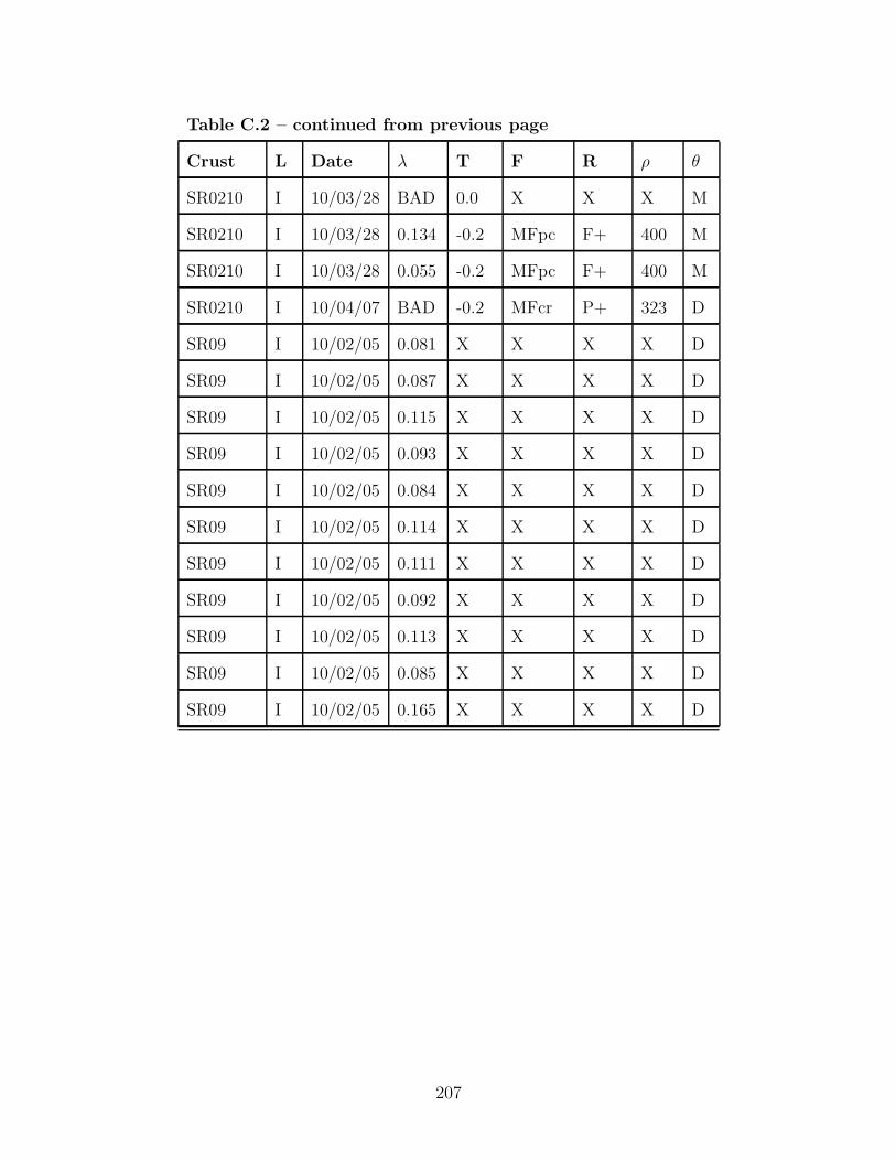
Table C.2 – continued from previous page
Crust L Date λ T F R ρ θ
SR0210 I 10/03/28 BAD 0.0 X X X M
SR0210 I 10/03/28 0.134 -0.2 MFpc F+ 400 M
SR0210 I 10/03/28 0.055 -0.2 MFpc F+ 400 M
SR0210 I 10/04/07 BAD -0.2 MFcr P+ 323 D
SR09 I 10/02/05 0.081 X X X X D
SR09 I 10/02/05 0.087 X X X X D
SR09 I 10/02/05 0.115 X X X X D
SR09 I 10/02/05 0.093 X X X X D
SR09 I 10/02/05 0.084 X X X X D
SR09 I 10/02/05 0.114 X X X X D
SR09 I 10/02/05 0.111 X X X X D
SR09 I 10/02/05 0.092 X X X X D
SR09 I 10/02/05 0.113 X X X X D
SR09 I 10/02/05 0.085 X X X X D
SR09 I 10/02/05 0.165 X X X X D
207

Table C.3: All thermal conductivity measurements. La-
bels and Units: Sample Location (A = Above; B = Be-
low; I = Crust Interior; V = Vertical through crust);
Thermal Conductivity (λ, [W m−1 k−1]); Goodness of
linear fit to rate of warming versus heating power (R2);
Average heating power during measurement (P,[W m−1]);
Duration of heating period used for calculation (∆t [s]);
Temperature rise during measurement (∆T [◦C])
Crust L Date λ R2 ∆t P ∆T
BV0112 A 10/01/31 0.078 0.995 35.4 0.383 1.4
BV0112 A 10/02/07 0.084 0.989 23.3 0.475 1.8
BV0112 A 10/02/15 0.082 0.998 47.5 0.447 1.5
BV0112 A 10/02/15 0.042 0.997 47.5 0.443 0.9
BV0112 A 10/03/01 BAD X X 0.455 0.0
BV0112 A 10/03/01 BAD X X 0.449 0.0
BV0112 A 10/03/08 0.095 0.993 35.4 0.445 1.3
BV0112 A 10/03/08 0.724 0.830 40.6 0.444 1.0
BV0112 A 10/03/14 BAD X X 0.419 0.0
BV0112 A 10/03/14 0.077 0.988 23.3 0.423 1.7
BV0112 A 10/03/23 BAD X X 0.563 0.0
BV0112 A 10/03/23 0.056 0.994 21.1 0.591 2.2
BV0112 B 10/01/31 0.100 0.981 20.9 0.372 1.8
BV0112 B 10/01/31 0.145 0.976 26.6 0.369 1.5
BV0112 B 10/01/31 0.104 0.985 24.5 0.366 1.6
X: Not recorded. *: Variable
208

Table C.3 – continued from previous page
Crust L Date λ R2 ∆t P ∆T
BV0112 B 10/02/07 BAD X X 0.000 0.0
BV0112 B 10/02/15 BAD X X 0.435 0.0
BV0112 B 10/02/15 0.058 0.987 45.3 0.432 1.0
BV0112 B 10/03/01 0.052 0.990 24.8 0.435 0.3
BV0112 B 10/03/01 BAD X X 0.423 0.0
BV0112 B 10/03/08 0.319 0.956 35.4 0.443 0.7
BV0112 B 10/03/08 0.189 0.962 23.3 0.439 1.3
BV0112 B 10/03/14 0.254 0.964 35.4 0.416 0.3
BV0112 B 10/03/14 BAD X X 0.413 0.0
BV0112 B 10/03/23 BAD X X 0.552 0.0
BV0112 B 10/03/23 BAD X X 0.544 0.0
BV0112 I 10/01/31 0.150 0.959 23.3 0.378 1.5
BV0112 I 10/01/31 0.193 0.958 29.7 0.375 1.2
BV0112 I 10/02/07 BAD X X 0.000 0.0
BV0112 I 10/02/15 0.209 0.964 29.7 0.439 0.9
BV0112 I 10/02/15 0.079 0.961 13.2 0.436 2.1
BV0112 I 10/03/01 BAD X X 0.440 0.0
BV0112 I 10/03/01 BAD X X 0.439 0.0
BV0112 I 10/03/08 0.062 0.995 47.5 0.442 1.8
BV0112 I 10/03/08 0.135 0.892 12.9 0.439 1.9
BV0112 I 10/03/14 BAD X X 0.422 0.0
BV0112 I 10/03/14 BAD X X 0.418 0.0
X: Not recorded. *: Variable
209

Table C.3 – continued from previous page
Crust L Date λ R2 ∆t P ∆T
BV0112 I 10/03/14 0.206 0.973 35.4 0.415 0.3
BV0112 I 10/03/14 0.317 0.000 47.5 0.416 0.2
BV0112 I 10/03/23 BAD X X 0.561 0.0
BV0112 I 10/03/23 BAD X X 0.559 0.0
BV0112 V 10/03/08 5.136 0.243 53.4 0.430 0.8
BV0112 V 10/03/14 0.279 0.991 106.5 0.411 0.3
BV0112 V 10/03/23 BAD X X 0.543 0.0
FI0110 A 10/01/10 0.108 0.993 35.4 0.762 3.2
FI0110 A 10/01/10 BAD X X 0.761 0.0
FI0110 A 12/01/10 0.118 0.986 59.8 0.360 1.6
FI0110 A 18/01/10 0.139 0.979 35.4 0.393 1.0
FI0110 A 18/01/10 0.147 0.966 29.7 0.388 1.0
FI0110 A 25/01/10 0.140 0.975 35.4 0.405 1.1
FI0110 A 25/01/10 0.160 0.988 45.3 0.398 0.9
FI0110 A 25/01/10 0.175 0.995 126.7 0.394 1.0
FI0110 A 02/02/10 0.161 0.989 45.3 0.416 0.9
FI0110 A 02/02/10 0.156 0.985 35.4 0.411 1.0
FI0110 A 02/02/10 0.201 0.982 40.6 0.407 0.9
FI0110 A 08/02/10 0.179 0.991 40.6 0.457 0.9
FI0110 A 08/02/10 0.205 0.985 40.6 0.454 0.9
FI0110 A 17/02/10 0.176 0.984 35.4 0.456 1.0
FI0110 A 17/02/10 0.213 0.966 26.9 0.453 0.8
X: Not recorded. *: Variable
210

Table C.3 – continued from previous page
Crust L Date λ R2 ∆t P ∆T
FI0110 A 28/02/10 0.208 0.969 47.5 0.484 0.8
FI0110 A 28/02/10 0.201 0.963 32.0 0.478 0.7
FI0110 A 09/03/10 0.192 0.984 45.3 0.039 0.9
FI0110 A 09/03/10 0.292 0.935 21.1 0.448 0.8
FI0110 A 15/03/10 0.212 0.991 56.9 0.435 0.6
FI0110 A 15/03/10 0.236 0.981 40.6 0.434 0.6
FI0110 A 10/03/22 0.222 0.901 17.2 0.477 0.8
FI0110 A 10/03/22 0.261 0.986 49.6 0.480 0.6
FI0110 A 10/03/28 BAD X X 0.000 0.0
FI0110 A 10/03/28 0.356 0.932 36.7 0.449 0.5
FI0110 A 10/04/07 0.354 0.918 27.9 0.503 0.7
FI0110 A 10/04/14 0.320 0.716 12.1 0.499 0.7
FI0110 A 10/04/14 BAD X X 0.475 0.0
FI0110 B 10/01/10 0.046 1.000 32.0 0.764 2.8
FI0110 B 10/01/10 0.040 0.999 50.0 0.762 4.3
FI0110 B 12/01/10 0.089 0.986 59.8 0.355 1.8
FI0110 B 12/01/10 0.096 0.986 29.7 0.352 1.4
FI0110 B 18/01/10 0.157 0.983 91.3 0.383 1.4
FI0110 B 18/01/10 0.104 0.991 35.4 0.378 1.2
FI0110 B 25/01/10 0.131 0.997 126.7 0.387 1.1
FI0110 B 25/01/10 0.129 0.991 35.4 0.382 1.1
FI0110 B 02/02/10 0.168 0.981 35.4 0.404 0.9
X: Not recorded. *: Variable
211

Table C.3 – continued from previous page
Crust L Date λ R2 ∆t P ∆T
FI0110 B 02/02/10 0.162 0.981 29.7 0.401 1.0
FI0110 B 02/02/10 0.161 0.987 40.6 0.399 0.9
FI0110 B 02/02/10 0.134 0.994 49.6 0.397 1.1
FI0110 B 08/02/10 0.166 0.989 35.4 0.450 1.0
FI0110 B 08/02/10 0.170 0.987 35.4 0.447 1.0
FI0110 B 17/02/10 0.148 0.996 34.7 0.449 0.7
FI0110 B 17/02/10 0.215 0.979 26.9 0.447 1.0
FI0110 B 28/02/10 0.200 0.995 24.8 0.469 0.6
FI0110 B 28/02/10 BAD X X 0.483 0.0
FI0110 B 09/03/10 0.275 0.916 26.6 0.441 0.7
FI0110 B 09/03/10 0.206 0.997 73.6 0.440 0.6
FI0110 B 15/03/10 0.216 0.990 53.4 0.439 0.6
FI0110 B 15/03/10 0.221 0.982 40.9 0.424 0.6
FI0110 B 10/03/22 0.296 0.977 40.6 0.483 0.6
FI0110 B 10/03/28 0.553 0.851 33.3 0.453 0.6
FI0110 B 10/03/28 0.489 0.840 35.4 0.457 0.5
FI0110 B 10/04/07 0.428 0.911 29.7 0.504 0.6
FI0110 B 10/04/14 0.467 0.960 45.3 0.493 0.5
FI0110 B 10/04/14 0.275 0.996 66.6 0.489 0.4
FI0110 I 08/02/10 0.188 0.985 48.3 0.444 0.9
FI0110 I 17/02/10 0.219 0.942 24.3 0.444 0.7
FI0110 I 28/02/10 0.175 0.976 21.8 0.476 0.7
X: Not recorded. *: Variable
212

Table C.3 – continued from previous page
Crust L Date λ R2 ∆t P ∆T
FI0110 I 28/02/10 0.209 0.981 19.4 0.472 0.8
FI0110 I 09/03/10 0.265 0.971 49.6 0.436 0.7
FI0110 I 09/03/10 BAD X X 0.437 0.0
FI0110 I 15/03/10 0.221 0.992 48.3 0.445 0.6
FI0110 I 15/03/10 0.282 0.805 16.3 0.441 0.6
FI0110 I 10/03/22 0.279 0.970 35.4 0.484 0.6
FI0110 I 10/03/22 0.258 0.976 40.6 0.480 0.7
FI0110 I 10/03/28 BAD X X 0.489 0.0
FI0110 I 10/03/28 0.843 0.593 40.6 0.470 0.6
FI0110 I 10/04/07 0.220 0.895 14.8 0.483 0.7
FI0110 I 10/04/14 BAD X X 0.477 0.0
FI0110 I 10/04/14 0.421 0.969 37.1 0.484 0.6
FI0308 A 10/03/15 0.106 0.997 47.5 0.445 1.1
FI0308 A 10/03/15 0.074 0.998 47.5 0.443 1.5
FI0308 A 10/03/22 0.115 0.993 35.4 0.505 1.3
FI0308 A 10/03/22 0.122 0.996 47.5 0.501 1.1
FI0308 A 10/03/28 0.130 0.999 76.1 0.506 0.9
FI0308 A 10/03/28 0.166 0.996 47.5 0.504 1.0
FI0308 A 10/04/07 0.203 0.949 17.1 0.501 0.8
FI0308 A 10/04/14 0.262 0.941 26.9 0.484 0.7
FI0308 A 10/04/14 0.290 0.954 35.4 0.485 0.7
FI0308 B 10/03/15 0.088 0.995 29.7 0.438 1.4
X: Not recorded. *: Variable
213

Table C.3 – continued from previous page
Crust L Date λ R2 ∆t P ∆T
FI0308 B 10/03/15 0.098 0.993 35.4 0.436 1.3
FI0308 B 10/03/22 0.143 0.985 23.3 0.496 1.1
FI0308 B 10/03/22 0.163 0.981 29.7 0.494 1.1
FI0308 B 10/03/28 0.158 0.981 29.7 0.502 1.2
FI0308 B 10/03/28 BAD X X 0.000 0.0
FI0308 B 10/04/07 0.243 0.980 35.4 0.503 0.8
FI0308 B 10/04/14 0.301 0.940 29.7 0.480 0.8
FI0308 B 10/04/14 0.256 0.956 35.4 0.479 0.8
FI0308 I 10/03/15 0.055 0.998 35.4 0.441 0.9
FI0308 I 10/03/15 0.239 0.966 35.4 0.439 1.0
FI0308 I 10/03/22 0.183 0.923 11.9 0.494 1.7
FI0308 I 10/03/22 0.204 0.980 35.4 0.498 1.3
FI0308 I 10/03/28 0.186 0.984 35.4 0.497 1.3
FI0308 I 10/03/28 2.103 0.024 8.6 0.503 1.6
FI0308 I 10/04/07 0.178 0.990 40.6 0.504 1.2
FI0308 I 10/04/14 0.133 0.943 13.2 0.483 2.0
FI0308 I 10/04/14 0.218 0.985 40.6 0.478 1.1
FI0308 V 10/03/15 0.102 0.994 35.4 0.451 1.1
FI0308 V 10/03/22 0.170 0.969 40.1 0.490 1.3
FI0308 V 10/03/28 0.290 0.916 34.3 0.480 1.0
FI0308 V 10/03/28 0.173 0.951 31.2 0.465 1.1
FI0308 V 10/04/07 0.180 0.965 12.1 0.740 1.2
X: Not recorded. *: Variable
214

Table C.3 – continued from previous page
Crust L Date λ R2 ∆t P ∆T
FI0308 V 10/04/14 0.233 0.933 23.3 0.481 0.6
FI0308 V 10/04/14 0.540 0.796 19.9 0.485 0.6
RP0112 A 10/01/19 0.100 0.975 29.7 0.395 1.4
RP0112 A 10/01/25 0.137 0.988 91.3 0.385 1.5
RP0112 A 10/02/02 0.144 0.989 45.3 0.404 1.0
RP0112 A 10/02/02 0.123 0.994 45.3 0.399 1.1
RP0112 A 10/02/09 0.129 0.996 47.5 0.446 1.0
RP0112 A 10/02/09 0.112 0.995 38.9 0.441 1.0
RP0112 A 10/02/15 0.118 0.993 18.2 0.430 0.7
RP0112 A 10/02/15 0.169 0.986 40.6 0.424 0.8
RP0112 A 10/02/27 0.199 0.973 29.7 0.470 1.0
RP0112 A 10/02/27 0.172 0.986 35.4 0.449 1.0
RP0112 A 10/03/08 0.164 0.992 35.4 0.431 0.8
RP0112 A 10/03/08 0.195 0.990 47.5 0.432 0.8
RP0112 A 10/03/14 0.193 0.993 57.0 0.434 0.8
RP0112 A 10/03/14 0.174 0.983 44.9 0.431 1.1
RP0112 A 10/03/23 0.330 0.979 57.0 0.534 0.9
RP0112 A 10/03/23 0.203 0.993 57.0 0.522 0.8
RP0112 A 10/03/29 1.107 0.863 46.6 0.534 0.2
RP0112 A 10/03/29 2.411 0.594 57.0 0.607 0.2
RP0112 A 10/03/29 BAD X X 0.561 0.0
RP0112 A 10/03/29 BAD X X 0.557 0.0
X: Not recorded. *: Variable
215

Table C.3 – continued from previous page
Crust L Date λ R2 ∆t P ∆T
RP0112 A 10/03/29 BAD X X 0.680 0.0
RP0112 A 10/04/06 BAD X X 0.482 0.0
RP0112 A 10/04/06 BAD X X 0.429 0.0
RP0112 A 10/04/13 0.267 0.991 103.8 0.550 1.6
RP0112 B 10/01/19 0.110 0.981 16.2 0.377 0.8
RP0112 B 10/01/25 0.154 0.989 91.3 0.369 1.2
RP0112 B 10/02/02 0.160 0.993 53.4 0.388 0.8
RP0112 B 10/02/02 0.158 0.991 45.3 0.385 0.9
RP0112 B 10/02/09 0.140 0.991 38.9 0.440 0.9
RP0112 B 10/02/09 0.125 0.991 17.8 0.436 0.8
RP0112 B 10/02/27 0.194 0.983 35.4 0.433 1.1
RP0112 B 10/02/27 0.196 0.978 35.4 0.431 0.8
RP0112 B 10/03/08 0.269 0.953 29.7 0.416 0.9
RP0112 B 10/03/08 0.228 0.985 47.5 0.415 0.8
RP0112 B 10/03/08 0.173 0.992 47.5 0.428 0.8
RP0112 B 10/03/08 0.147 0.992 47.5 0.420 0.9
RP0112 B 10/03/14 0.192 0.990 57.0 0.434 0.7
RP0112 B 10/03/14 0.196 0.992 57.0 0.426 0.6
RP0112 B 10/03/23 0.359 0.978 57.0 0.531 0.7
RP0112 B 10/03/23 0.408 0.965 47.5 0.521 0.7
RP0112 B 10/03/29 BAD X X 0.521 0.0
RP0112 B 10/03/29 BAD X X 0.513 0.0
X: Not recorded. *: Variable
216
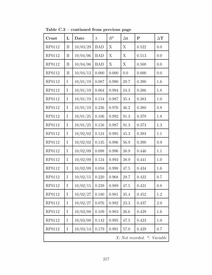
Table C.3 – continued from previous page
Crust L Date λ R2 ∆t P ∆T
RP0112 B 10/03/29 BAD X X 0.522 0.0
RP0112 B 10/04/06 BAD X X 0.513 0.0
RP0112 B 10/04/06 BAD X X 0.500 0.0
RP0112 B 10/04/13 0.000 0.000 0.0 0.000 0.0
RP0112 I 10/01/19 0.087 0.990 29.7 0.390 1.6
RP0112 I 10/01/19 0.064 0.994 24.3 0.386 1.8
RP0112 I 10/01/19 0.154 0.987 35.4 0.383 1.0
RP0112 I 10/01/19 0.236 0.976 46.2 0.380 0.8
RP0112 I 10/01/25 0.106 0.992 91.3 0.379 1.8
RP0112 I 10/01/25 0.156 0.987 91.3 0.373 1.3
RP0112 I 10/02/02 0.124 0.995 45.3 0.393 1.1
RP0112 I 10/02/02 0.135 0.996 56.9 0.390 0.9
RP0112 I 10/02/09 0.098 0.996 38.9 0.446 1.1
RP0112 I 10/02/09 0.124 0.993 38.9 0.441 1.0
RP0112 I 10/02/09 0.058 0.998 47.5 0.434 1.6
RP0112 I 10/02/15 0.220 0.968 29.7 0.422 0.7
RP0112 I 10/02/15 0.239 0.989 47.5 0.421 0.8
RP0112 I 10/02/27 0.180 0.981 35.4 0.452 1.2
RP0112 I 10/02/27 0.076 0.992 23.3 0.437 2.0
RP0112 I 10/03/08 0.109 0.983 26.6 0.429 1.6
RP0112 I 10/03/08 0.142 0.995 47.5 0.423 1.0
RP0112 I 10/03/14 0.179 0.991 57.0 0.429 0.7
X: Not recorded. *: Variable
217

Table C.3 – continued from previous page
Crust L Date λ R2 ∆t P ∆T
RP0112 I 10/03/14 0.139 0.995 57.0 0.425 0.8
RP0112 I 10/03/23 BAD X X 0.528 0.0
RP0112 I 10/03/23 0.079 0.995 75.0 0.526 1.4
RP0112 I 10/03/29 BAD X X 0.519 0.0
RP0112 I 10/03/29 BAD X X 0.523 0.0
RP0112 I 10/04/06 BAD X X 0.487 0.0
RP0112 I 10/04/06 BAD X X 0.498 0.0
RP0112 I 10/04/13 0.000 0.000 0.0 0.000 0.0
RP0112 V 10/03/08 0.124 0.985 39.1 0.409 1.2
RP0112 V 10/03/08 0.117 0.978 29.4 0.411 1.7
RP0112 V 10/03/14 0.180 0.995 138.8 0.419 0.8
RP0112 V 10/03/14 0.213 0.979 81.8 0.416 1.0
RP0112 V 10/03/23 BAD X X 0.529 0.0
RP0112 V 10/03/23 0.204 0.990 114.6 0.568 1.1
RP0112 V 10/03/29 BAD X X 0.796 0.0
RP0112 V 10/04/06 BAD X X 0.484 0.0
RP0112 V 10/04/06 BAD X X 0.467 0.0
RP0112 V 10/04/13 0.000 0.000 0.0 0.000 0.0
LAB0312 I 13 12:00 BAD X X 0.432 0.0
LAB0312 I 13 12:37 0.089 0.919 9.0 0.433 0.3
LAB0312 I 13 12:51 0.141 0.890 4.4 0.425 0.3
LAB0312 I 13 13:26 0.648 0.901 49.9 0.421 0.1
X: Not recorded. *: Variable
218

Table C.3 – continued from previous page
Crust L Date λ R2 ∆t P ∆T
LAB0312 I 13 14:05 0.276 0.969 40.0 0.413 0.2
LAB0312 I 13 15:10 0.142 0.996 52.1 0.421 0.7
LAB0330 A 30 09:30 BAD X X 0.569 0.0
LAB0330 B 30 09:30 BAD X X 0.559 0.0
LAB0330 I 30 09:30 BAD X X 0.567 0.0
LAB0330 I 30 09:30 BAD X X 0.562 0.0
LAB0330 V 30 09:30 0.094 0.769 4.6 0.555 3.0
LAB0330 V 30 10:30 0.034 0.995 13.2 0.546 1.6
LAB0330 V 30 10:30 0.065 0.979 13.2 0.541 0.8
LAB0330 V 30 12:20 0.285 0.979 31.2 0.571 0.3
LAB0330 V 30 12:20 BAD X X 0.565 0.0
LAB0330 V 30 14:12 0.249 0.927 19.2 0.527 0.3
LAB0330 V 30 14:12 BAD X X 0.522 0.0
LAB0330 V 30 16:55 0.122 0.987 71.3 0.527 1.8
LAB0330 V 30 16:55 0.193 0.975 83.8 0.521 1.9
LAB0330 V 30 21:50 0.236 0.989 85.7 0.546 1.5
LAB0330 V 30 21:50 0.250 0.978 81.8 0.538 1.6
LAB0330 V 31 07:25 0.000 0.000 0.0 0.000 0.0
LAB0330 V 31 07:25 0.000 0.000 0.0 0.000 0.0
LAB0409 V 10 13:00 BAD X X 0.486 0.0
LAB0409 V 09 13:00 0.072 0.816 4.6 0.496 2.5
LAB0409 V 09 19:35 BAD X X 0.491 0.0
X: Not recorded. *: Variable
219

Table C.3 – continued from previous page
Crust L Date λ R2 ∆t P ∆T
LAB0409 V 09 19:35 0.690 0.910 45.2 0.491 0.4
LAB0409 V 10 01:15 0.136 0.995 52.1 0.499 0.8
LAB0409 V 10 01:15 0.252 0.963 40.0 0.497 0.4
LAB0409 V 10 08:20 0.130 0.988 17.8 0.471 1.1
LAB0409 V 10 08:20 0.286 0.971 81.8 0.480 1.5
LAB0409 V 10 14:30 0.270 0.979 81.8 0.496 1.2
LAB0410 V 10 19:15 0.058 0.997 47.0 -0.282 3.3
LAB0410 V 10 19:15 0.025 1.000 52.1 0.533 2.8
LAB0410 V 11 09:30 0.081 0.967 25.2 0.521 1.7
LAB0410 V 11 09:30 0.178 0.988 95.9 0.523 1.6
LAB0410 V 11 21:00 0.277 0.966 69.1 0.518 1.8
LAB0410 V 11 21:00 0.302 0.987 109.1 0.515 1.2
LAB0410 V 12 09:40 BAD X X 0.511 0.0
LAB0410 V 12 09:40 0.269 0.780 71.3 0.460 1.6
LAB0410 V 12 21:05 0.225 0.986 54.8 0.517 1.4
LAB0410 V 12 21:05 0.246 0.987 109.1 0.512 1.9
LAB0410 V 13 09:35 0.273 0.987 100.5 0.550 1.7
LAB0410 V 13 09:35 0.409 0.000 91.1 0.546 1.7
LAB0413 V 10/04/13 0.080 0.997 50.3 0.520 1.7
LAB0413 V 10/04/13 BAD X X 0.514 0.0
LAB0413 V 10/04/14 BAD X X 0.559 0.0
LAB0413 V 10/04/14 0.293 0.968 91.1 0.538 0.7
X: Not recorded. *: Variable
220
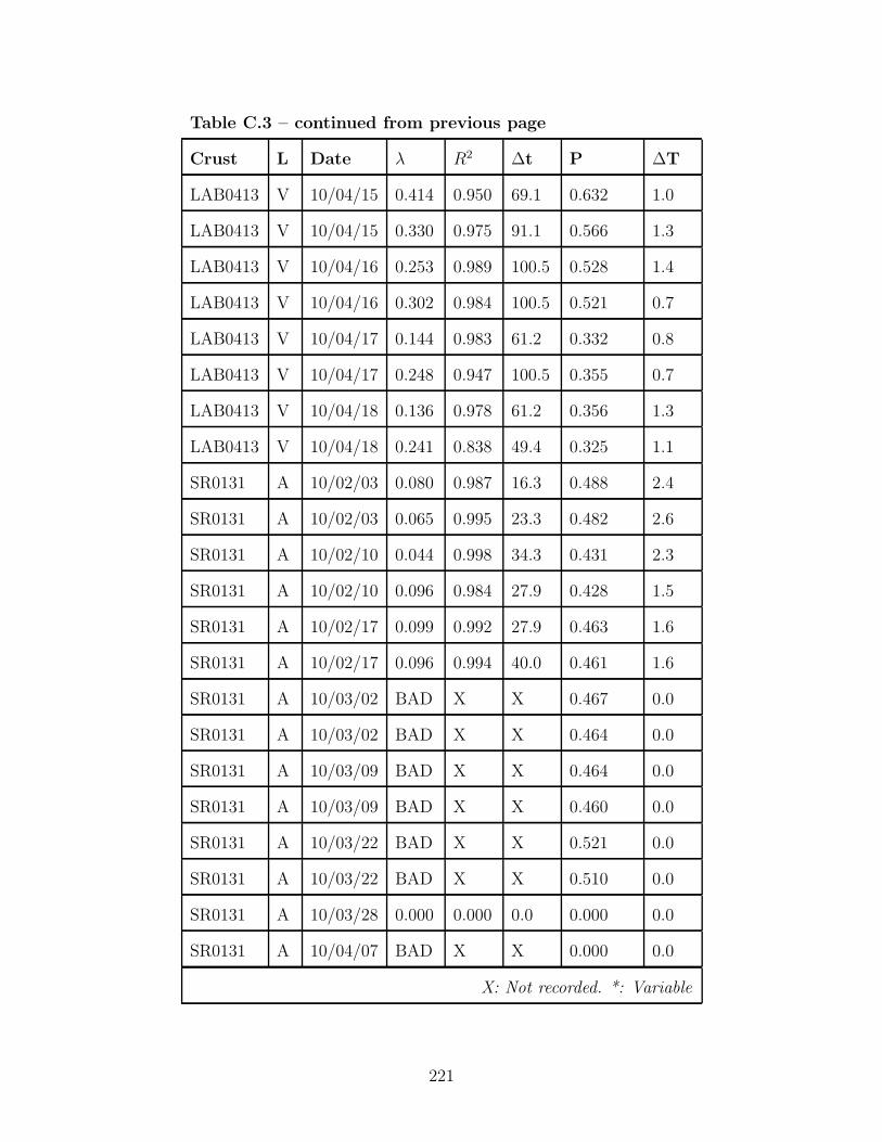
Table C.3 – continued from previous page
Crust L Date λ R2 ∆t P ∆T
LAB0413 V 10/04/15 0.414 0.950 69.1 0.632 1.0
LAB0413 V 10/04/15 0.330 0.975 91.1 0.566 1.3
LAB0413 V 10/04/16 0.253 0.989 100.5 0.528 1.4
LAB0413 V 10/04/16 0.302 0.984 100.5 0.521 0.7
LAB0413 V 10/04/17 0.144 0.983 61.2 0.332 0.8
LAB0413 V 10/04/17 0.248 0.947 100.5 0.355 0.7
LAB0413 V 10/04/18 0.136 0.978 61.2 0.356 1.3
LAB0413 V 10/04/18 0.241 0.838 49.4 0.325 1.1
SR0131 A 10/02/03 0.080 0.987 16.3 0.488 2.4
SR0131 A 10/02/03 0.065 0.995 23.3 0.482 2.6
SR0131 A 10/02/10 0.044 0.998 34.3 0.431 2.3
SR0131 A 10/02/10 0.096 0.984 27.9 0.428 1.5
SR0131 A 10/02/17 0.099 0.992 27.9 0.463 1.6
SR0131 A 10/02/17 0.096 0.994 40.0 0.461 1.6
SR0131 A 10/03/02 BAD X X 0.467 0.0
SR0131 A 10/03/02 BAD X X 0.464 0.0
SR0131 A 10/03/09 BAD X X 0.464 0.0
SR0131 A 10/03/09 BAD X X 0.460 0.0
SR0131 A 10/03/22 BAD X X 0.521 0.0
SR0131 A 10/03/22 BAD X X 0.510 0.0
SR0131 A 10/03/28 0.000 0.000 0.0 0.000 0.0
SR0131 A 10/04/07 BAD X X 0.000 0.0
X: Not recorded. *: Variable
221

Table C.3 – continued from previous page
Crust L Date λ R2 ∆t P ∆T
SR0131 B 10/02/03 0.149 0.974 23.3 0.470 1.5
SR0131 B 10/02/03 0.142 0.985 23.3 0.467 1.5
SR0131 B 10/02/10 0.073 0.994 23.3 0.421 1.6
SR0131 B 10/02/10 0.080 0.931 13.2 0.419 1.9
SR0131 B 10/02/17 0.165 0.970 23.3 0.454 1.2
SR0131 B 10/02/17 0.131 0.994 47.5 0.452 1.0
SR0131 B 10/03/02 3.640 0.491 70.1 0.461 0.5
SR0131 B 10/03/02 1.727 0.634 52.1 0.459 0.6
SR0131 B 10/03/09 BAD X X 0.451 0.0
SR0131 B 10/03/09 BAD X X 0.448 0.0
SR0131 B 10/03/22 BAD X X 0.503 0.0
SR0131 B 10/03/22 BAD X X 0.500 0.0
SR0131 B 10/03/28 0.000 0.000 0.0 0.000 0.0
SR0131 B 10/04/07 BAD X X 0.000 0.0
SR0131 I 10/02/03 0.714 0.459 8.6 0.478 1.7
SR0131 I 10/02/03 0.148 0.939 16.3 0.474 1.6
SR0131 I 10/02/10 0.311 0.625 13.2 0.426 1.2
SR0131 I 10/02/10 0.109 0.924 10.9 0.423 1.2
SR0131 I 10/02/17 0.158 0.971 23.3 0.458 1.5
SR0131 I 10/02/17 0.175 0.981 34.3 0.456 1.3
SR0131 I 10/03/02 0.000 0.000 0.0 0.000 0.0
SR0131 I 10/03/09 BAD X X 0.454 0.0
X: Not recorded. *: Variable
222

Table C.3 – continued from previous page
Crust L Date λ R2 ∆t P ∆T
SR0131 I 10/03/09 BAD X X 0.448 0.0
SR0131 I 10/03/22 BAD X X 0.155 0.0
SR0131 I 10/03/22 BAD X X 0.505 0.0
SR0131 I 10/03/28 BAD X X 0.525 0.0
SR0131 I 10/03/28 0.134 0.976 23.3 0.529 0.3
SR0131 I 10/03/28 0.055 0.999 36.7 0.516 1.9
SR0131 I 10/04/07 BAD X X 0.000 0.0
SR0210 A 10/02/10 0.000 0.000 0.0 0.000 0.0
SR0210 A 10/02/17 0.092 0.990 24.5 0.474 2.0
SR0210 A 10/02/17 0.091 0.982 17.2 0.471 2.1
SR0210 A 10/03/02 BAD X X 0.475 0.0
SR0210 A 10/03/02 0.082 0.995 34.3 0.470 1.9
SR0210 A 10/03/09 0.022 0.997 47.5 0.468 2.0
SR0210 A 10/03/09 BAD X X 0.464 0.0
SR0210 A 10/03/22 BAD X X 0.522 0.0
SR0210 A 10/03/22 BAD X X 0.518 0.0
SR0210 A 10/03/28 0.000 0.000 0.0 0.000 0.0
SR0210 A 10/04/07 0.000 0.000 0.0 0.000 0.0
SR0210 B 10/02/10 0.044 0.998 34.3 0.431 2.3
SR0210 B 10/02/10 0.096 0.984 27.9 0.428 1.5
SR0210 B 10/02/17 0.099 0.992 27.9 0.463 1.6
SR0210 B 10/02/17 0.096 0.994 40.0 0.461 1.6
X: Not recorded. *: Variable
223
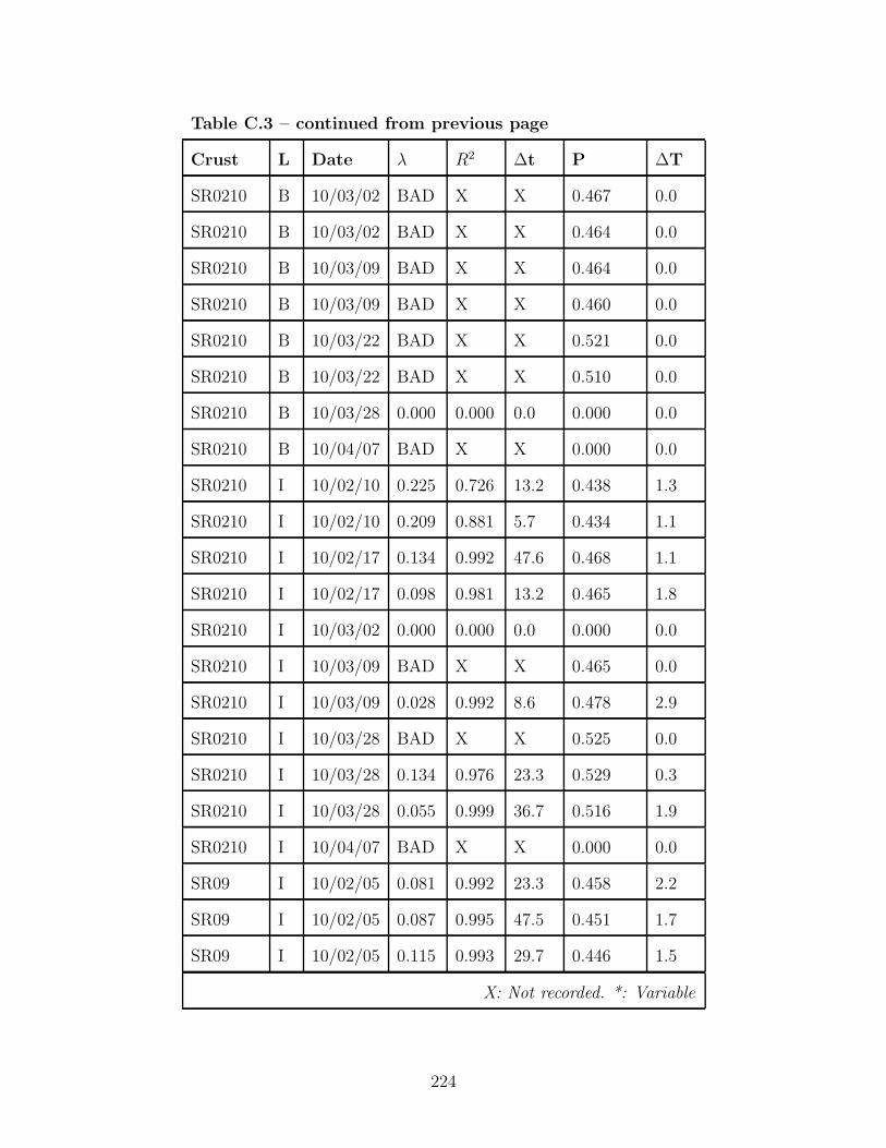
Table C.3 – continued from previous page
Crust L Date λ R2 ∆t P ∆T
SR0210 B 10/03/02 BAD X X 0.467 0.0
SR0210 B 10/03/02 BAD X X 0.464 0.0
SR0210 B 10/03/09 BAD X X 0.464 0.0
SR0210 B 10/03/09 BAD X X 0.460 0.0
SR0210 B 10/03/22 BAD X X 0.521 0.0
SR0210 B 10/03/22 BAD X X 0.510 0.0
SR0210 B 10/03/28 0.000 0.000 0.0 0.000 0.0
SR0210 B 10/04/07 BAD X X 0.000 0.0
SR0210 I 10/02/10 0.225 0.726 13.2 0.438 1.3
SR0210 I 10/02/10 0.209 0.881 5.7 0.434 1.1
SR0210 I 10/02/17 0.134 0.992 47.6 0.468 1.1
SR0210 I 10/02/17 0.098 0.981 13.2 0.465 1.8
SR0210 I 10/03/02 0.000 0.000 0.0 0.000 0.0
SR0210 I 10/03/09 BAD X X 0.465 0.0
SR0210 I 10/03/09 0.028 0.992 8.6 0.478 2.9
SR0210 I 10/03/28 BAD X X 0.525 0.0
SR0210 I 10/03/28 0.134 0.976 23.3 0.529 0.3
SR0210 I 10/03/28 0.055 0.999 36.7 0.516 1.9
SR0210 I 10/04/07 BAD X X 0.000 0.0
SR09 I 10/02/05 0.081 0.992 23.3 0.458 2.2
SR09 I 10/02/05 0.087 0.995 47.5 0.451 1.7
SR09 I 10/02/05 0.115 0.993 29.7 0.446 1.5
X: Not recorded. *: Variable
224

Table C.3 – continued from previous page
Crust L Date λ R2 ∆t P ∆T
SR09 I 10/02/05 0.093 0.968 16.3 0.441 1.8
SR09 I 10/02/05 0.084 0.992 23.3 0.437 1.9
SR09 I 10/02/05 0.114 0.974 23.3 0.420 1.8
SR09 I 10/02/05 0.111 0.993 35.4 0.434 1.3
SR09 I 10/02/05 0.092 0.988 23.3 0.430 1.5
SR09 I 10/02/05 0.113 0.982 23.3 0.428 1.5
SR09 I 10/02/05 0.085 0.963 8.6 0.427 2.2
SR09 I 10/02/05 0.165 0.982 35.4 0.423 1.2
225
Related Documents