Track Extrapolation/Shower Reconstruction in a Digital HCAL – ANL Approach Steve Magill ANL 1 st step - Track extrapolation thru Cal – substitute for Cal.

Track Extrapolation/Shower Track Extrapolation/Shower Reconstruction in a Digital HCAL – ANL Reconstruction in a Digital HCAL – ANL

ApproachApproach

Steve Magill ANL

1st step - Track extrapolation thru Cal

– substitute for Cal cells in road (core + tuned outlyers)

- analog* or digital techniques in HCAL – S. Magill

– Cal granularity/segmentation optimized for separation of charged/neutral clusters

2nd step - Photon finder (use analytic long./trans. energy

profiles, ECAL shower max, etc.) – S. Kuhlmann

3rd step - Jet Algorithm on tracks and photons - Done

4th step – include remaining Cal cells (neutral hadron

energy) in jet (cone?) -> Digital HCAL?

E-flow alg. Korea, NIU, Prague

* V. Morgunov, CALOR2002

Density-Weighted CAL CellsDensity-Weighted CAL Cells

cell density weight = 3/40

area ~ 40 cells

red – E fraction for density > 1/#blue – E fraction outside .04 cone

# cells in window

E-weight : analog calD-weight : digital cal

Study with single 10 GeV pions

Why 40 cells?

So far, 2D density (each layer)

D-Weights ECAL Interaction Layer 20, Theta, D-Weights ECAL Interaction Layer 20, Theta, PhiPhi

Gaussian fits

D-Weights HCAL Interaction Layer 10, Theta, D-Weights HCAL Interaction Layer 10, Theta, PhiPhi

Gaussian fits

Density vs E - ECALDensity vs E - ECAL

MIP signal – 8 MeV

cell density

cell

energ

y (

GeV

)

Density vs E - HCALDensity vs E - HCAL

MIP signal – 36 MeV

what’s this?

cell

energ

y (

GeV

)

cell density

Mokka, impact of the gas in HCALElectrons PionsGas GasScin Scin

HCAL E fraction, Ecell > 1 MIPHCAL E fraction, Ecell > 1 MIP

Importance of threshold level-> need to vary in test beam for scintillator cal

HCAL Cell Density Distribution (40 cell HCAL Cell Density Distribution (40 cell window)window)

31% single cell windows

mean ~ 4 cells

Seed Cell Distribution (cell density > 1/40)Seed Cell Distribution (cell density > 1/40)

-> in 1 layer

ECAL int. layer 20 HCAL int. layer 10

0.05 0.10 0.15 0.20 0.25 0.30 0.35 0.40 0.45 0.50 0.55 0.60 0.65 0.70 0.75 0.80 0.85 0.90 0.950

10

20

30

40

50

60

70

80

90

100

110

120

130

140

150

160

170

180

190

200 entries : 2463.0 min : 0.024523 max : 0.95608 mean : 0.73240 rms : 0.11537

Fraction of Total Energy in Seeds

Energy fraction in seedsEnergy fraction in seeds

~73% of energy in seed cells

0.0 0.1 0.2 0.3 0.4 0.5 0.6 0.7 0.8 0.9 1.00

10

20

30

40

50

60

70

80

90

100

110

120

130 entries : 2463.0 min : 0 max : 1.0000 mean : 0.57425 rms : 0.18038

Total Energy fraction in 04 cone

0.0 0.1 0.2 0.3 0.4 0.5 0.6 0.7 0.8 0.9 1.00

10

20

30

40

50

60

70

80

90

100

110

120

130

140

150

160

170

180

190

200 entries : 2463.0 min : 0 max : 1.0000 mean : 0.78574 rms : 0.12406

Total Energy fraction in 1 cone

Total Energy fraction in fixed cones (SNARK?)Total Energy fraction in fixed cones (SNARK?)

Cone size 0.04

Cone size 0.1

TTrack rack EExtrapolation/xtrapolation/SShower hower LLink ink AAlgorithmlgorithm

1. Pick up all seed cells close to extrapolated track- Can tune for optimal seed cell definition- For cone size < 0.1 (~6o), get 85% of energy

2. Add cells in a cone around each seed cell through n layers

3. Linked seed cells in subsequent cones form the reconstructed shower4. Discard all cells linked to the track

Of course, neutrals are NNon-on-LLinked inked CCellsells

Single 10 GeV Pion : D-weighted event displaySingle 10 GeV Pion : D-weighted event display

Blue – allRed – density > 1Green – density > 3

Gap between ECAL/HCAL

Single 10 GeV Pion – event display Single 10 GeV Pion – event display comparisoncomparison

Photon Analysis (S. Kuhlmann)Photon Analysis (S. Kuhlmann)

1. Cluster EM cells with cone algorithm of radius < 0.04 radians

2. Remove a cluster if a track points to within 0.03 radians, or, if the cluster is a mip in all 30 layers, remove if within 0.01 radians of a track

3. Require shower max energy deposit > 30 MeV (layers 8,9,10 summed)

4. Remove cluster if EEM/Etrack < 0.1 AND R < 0.1 (gets rid of charged pion fragments)

Remaining clusters classified as “Photons”

Mean=0.25 GeV, Width=2.8 GeV, Perfect EFLOW Goal is 1.4 GeV.

(Mean=1.2 GeV, Width = 3.1 GeV without the “box” cut on EM/Track Ratio and Delta-R)

Hadronic Z Decays at s = 91 GeV

Total Photon Energy - Total Monte Carlo Photons (GeV)

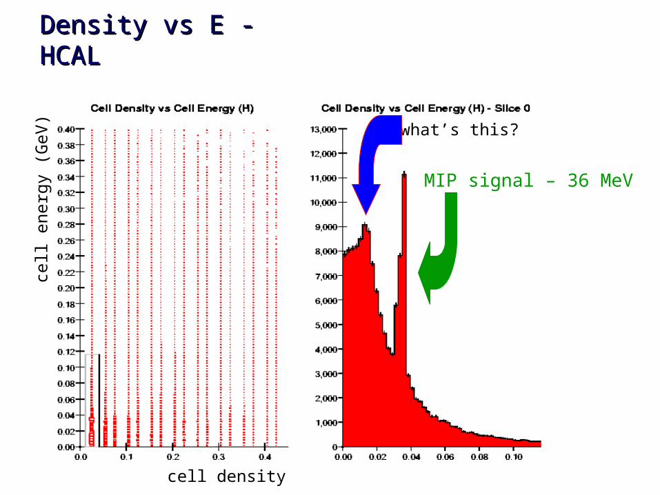
How the Tesla TDR analysis was done JC Brient (Billy Bob’s version)

Photons

1) Extrapolate tracks thru the first 12 layers of EM (6 X0 for Tesla) 2) Remove the single cell in each layer that the track hit (1 cm x 1cm cells for Tesla) 3) Take all the remaining hits in the first 12 layers and sum them in theta-phi with

no other clustering, exp(-7/9 * 6)=0.0094 means >99% of the photons convert. 4) Order in energy. These are now the seeds for the rest of the EM calorimeter. 5) Do nearest neighbor clustering in all 40 layers using these seeds. Of course

remove seeds from the list as they are absorbed into previous clusters. 6) Apply a chisq-type cut (not too critical since steps 3 and 4 are effectively a

shower max cut, and charged particle fragments only in the latter 2/3 of the EM calorimeter are ignored because they didn’t have a seed).

SummarySummary

1. Continuing work on implementation and tuning of shower link algorithm

2. Tune to single particles first, then to particles in jets

3. Add photons

4. Compare to analog version (SNARK)

5. Use final EFA to optimize transverse cell size of digital

HCAL in SD, LD, TESLA detectors