Experimental Investigation of Void Fraction During Horizontal Flow in Larger Diameter Refrigeration Applications M. J. Wilson, T. A. Newell, and J. C. Chato ACRC TR-I40 For additional information: Air Conditioning and Refrigeration Center University of Illinois Mechanical & Industrial Engineering Dept. 1206 West Green Street 1206 West Green Street Urbana, IL 61801 (217) 333-3115 July 1998 Prepared as part of ACRC Project 74 Experimental Investigation of Void Fraction During Refrigerant Condensation and Evaporation T. A. Newell and J. C. Chato, Principal Investigators

Welcome message from author
This document is posted to help you gain knowledge. Please leave a comment to let me know what you think about it! Share it to your friends and learn new things together.
Transcript

Experimental Investigation of Void Fraction During Horizontal Flow in Larger Diameter
Refrigeration Applications
M. J. Wilson, T. A. Newell, and J. C. Chato
ACRC TR-I40
For additional information:
Air Conditioning and Refrigeration Center University of Illinois Mechanical & Industrial Engineering Dept. 1206 West Green Street 1206 West Green Street Urbana, IL 61801
(217) 333-3115
July 1998
Prepared as part of ACRC Project 74 Experimental Investigation of Void Fraction
During Refrigerant Condensation and Evaporation T. A. Newell and J. C. Chato, Principal Investigators

The Air Conditioning and Refrigeration Center was founded in 1988 with a grant from the estate of Richard W. Kritzer, thefounder of Peerless of America Inc. A State of Illinois Technology Challenge Grant helped build the laboratory facilities. The ACRC receives continuing support from the Richard W. Kritzer Endowment and the National Science Foundation. The following organizations have also become sponsors of the Center.
Amana Refrigeration, Inc. Brazeway, Inc. Carrier Corporation Caterpillar, Inc. Copeland Corporation Dayton Thermal Products Delphi Harrison Thermal Systems Eaton Corporation Ford Motor Company Frigidaire Company General Electric Company Hill PHOENIX Hydro Aluminum Adrian, Inc. Indiana Tube Corporation Lennox International, Inc. Modine Manufacturing Co. Peerless of America, Inc. The Trane Company Whirlpool Corporation York International, Inc.
For additional information:
Air Conditioning & Refrigeration Center Mechanical & Industrial Engineering Dept. University of Illinois 1206 West Green Street Urbana IL 61801
2173333115

Abstract
EXPERIMENTAL INVESTIGATION OF VOID FRACTION DURING HORIZONTAL FLOW IN LARGER DIAMETER REFRIGERATION APPLICATIONS
Michael Jay Wilson Department of Mechanical and Industrial Engineering
University oflllinois at Urbana-Champaign, 1998 Ty Newell and John C. Chato, Advisors
Void fractions were measured for R134a and R410A for a smooth tube with inside
diameter of 6.12 mm (0.241"), an axially grooved tube of base diameter 8.89 mm
(0.350"), and a 18° helically grooved of base diameter 8.93 mm (0.352"). The experiment
covered mass fluxes from 75 kg/m2s to 700 kg/m2s (55 - 515 klbnJ'ft2-hr) and average test
section qualities from 5% to 99% with an inlet temperature of 5°C (41°F). Several
existing models are examined for accuracy and a simple adjusted model is presented to
accurately predict the data and data presented in a companion study by Yashar[1998].
The experimental apparatus and methodology are also discussed.
iii


Table of Contents
Page
List of Tables ............................................................................................................ viii
List of Figures ........................................................................................................... ix
Nomenclature ........................................................................................................... xx
Chapter
I Introduction ............................................................................................................ 1
2 Literature Review ................................................................................................... 2
2.1- Homogenous. '" .............................................................................................. 2
2.2- Slip Ratio ....................................................................................................... 2
2.2.1- Rigot Correlation .................................................................................. 3
2.2.2- Zivi Correlation .................................................................................... 3
2.2.3- Smith Correlation ................................................................................. 4
2.2.4- Ahrens-Thorn Correlation ..................................................................... 5
2.2.5- Levy Correlation ................................................................................... 6
2.3- Lockhart-Martinelli. ........................................................................................ 6
2.3.1- Baroczy Correlation .............................................................................. 7
2.3.2- Wallis Correlation ................................................................................. 7
2.4 Mass Flux Dependent ....................................................................................... 8
2.4.1- Tandon Correlation ............................................................................... 8
2.4.2- Premoli Correlation ............................................................................... 9
2.4.3- Hughmark Correlation ......................................................................... 10
2.4.4- Graham's Condenser Correlation ........................................................ II
3 Experimental Facilities and Measurement Techniques ............................................ 13
3.1- Experimental Test Facility ............................................................................. 13
3.1.1- Refrigerant Loop ................................................................................ 13
3.1.2- Chiller ................................................................................................. 14
3.1.3- Test Section ........................................................................................ 15
3.2- Data Acquisition System ............................................................................... 16
3.3- Instrumentation and Measurements ............................................................... 17
3.3.1- Temperature Measurements ................................................................ 17
3.3.2- Pressure Measurements ....................................................................... 17
3.3.3- Mass Flow Measurements ................................................................... 18
v

3.3.4- Power Measurements .......................................................................... 18
3.3.5- Calculated Parameters ......................................................................... 19
4 Experimental Procedure and Data Reduction ........................................................ 25
4.1- Test Section Volumes ................................................................................... 25
4.2- Void Fraction Calculations ............................................................................ 26
4.3- Uncertainty Analysis ..................................................................................... 28
5 Smooth Tube Experimental Results ....................................................................... 30
5.1- Void Fraction Results .................................................................................... 30
5.1.1- Effect of Refrigerant on Void Fraction ................................................ 30
5.1.2- Effect of Mass Flux on Void Fraction ................................................. 30
5.1.3- Effect of Heat Flux on Void Fraction .................................................. 31
5.1.4- Effect of Diameter on Void Fraction ................................................... 31
5.2- Correlation Comparison ................................................................................. 32
5.2.1- Slip Ratio Correlations ........................................................................ 32
5.2.2- Lockhart-Martinelli Correlations ......................................................... 33
5.2.3- Flux Dependent Correlations ............................................................... 33
5.2.4- Diameter Effects on the Correlations ................................................... 34
6 Axially Grooved Experimental Results .................................................................. 44
6.1- Void Fraction Results ................................................................................... 44
6.1.1- Effect of Refrigerant on Void Fraction ................................................ 44
6.1.2- Effect of Mass Flux on Void Fraction ................................................. 44
6.1.3- Effect of Heat Flux on Void Fraction ................................ '" ............... 45
6.1.4- Effect of Diameter on Void Fraction ................................................... 45
6.1.5- Effect of Micro-fins on Void Fraction ................................................. 45
6.2- Correlation Comparisons .............................................................................. 46
7 Helically Grooved Tube Results ............................................................................ 56
7.1- Void Fraction Results ................................................................................... 56
7.1.1- Effect of Refrigerant on Void Fraction ................................................ 56
7.1.2- Effect of Mass Flux on Void Fraction ................................................. 56
7.1.3- Effect of Heat Flux on Void Fraction .................................................. 57
7.1.4- Effect of Diameter on Void Fraction ................................................... 57
7.1.5- Effect of Tube Enhancements on Void Fraction .................................. 57
7.2- Correlation Comparisons .............................................................................. 58
8 Conclusions and Recommendations ....................................................................... 68
8.1- Mass Flux Independence or Dependence ....................................................... 68
8.2 - Correlation Recommendation ........................................................................ 69
vi

8.2.1- Adjusted Premoli Correlation .............................................................. 70
8.2.1.1- Smooth Tubes ......................................................................... 71
8.2.1.2- Axially Grooved Tubes ............................................................. 71
8.2.1.3- Helically Grooved Tubes .......................................................... 72
8.2.2- Froude Rate Correlations .................................................................... 72
8.2.2.1- Smooth Tubes ......................................................................... 72
8.2.2.2- Axially Grooved Tubes ............................................................ 73
8.2.2.3- Helically Grooved Tubes .......................................................... 74
8.3- Conclusions .................................................................................................. 75
Bibliography ............................................................................................................. 84
Appendix A Smooth Tubes ...................................................................................... 87
Appendix B Axially Grooved Tubes ....................................................................... 102
Appendix C Helically Grooved Tubes .................................................................... 118
Appendix D Conclusion Plots ................................................................................ 134
vii


List of Tables
Table Page
2.1 Ahrens-Thorn Correlations ................................................................................... 5
2.2 Baroczy Correlation ............................................................................................. 7
2.3 Hughmark flow parameter K as a function of Z .................................................. 11
3.1 Dimensions of grooved tubes............................................................................. 15
4.1 Void fraction uncertainty for given quality range and tube .................................. 28
A.1 Raw data for 6.12 mm inner diameter smooth tube ............................................ 88
B.1 Raw data for 8.89 mm base diameter axially grooved tube ............................... 103
C.1 Raw data for 8.93 mm base diameter helically grooved tube ............................ 119
viii


List of Figures
Figure Page
3.1 Schematic of refrigerant loop ............................................................................. 20
3.2 Chiller system .................................................................................................... 20
3.3 Micro-fm tubes dimensions and features for 8.93 mm inner diameter micro-finned test section ............................................................................................... 21
3.4 Test section dimensions and features ................................................................... 22
3.5 Void fraction tap where OD is the outside diameter of the test section the tap will fit on to .................................................................................................. 22
3.6 Pressure tap where OD is the outside diameter of the test section the tap will fit on to ........................................................................................................ 23
3.7 Thermocouple placement in thick walled tubes .................................................... 23
3.8 Thermocouple placement in thin walled tubes ...................................................... 24
4.1 Example error analysis plot for the helically grooved tube ................................... 29
5.1 Void fraction vs. average quality 6.12 mm inner diameter smooth tube ................ 35
5.2 Void fraction vs. average quality using R134a in 6.12 mm inner diameter smooth tube. Mass flux (G) given in kglm2s ...................................................... 35
5.3 Void fraction vs. average quality using R410A in 6.12 mm inner diameter smooth tube. Mass flux (G) given in kglm2s ....................................................... 36
5.4 Void fraction vs. average quality using R134a in a 6.12 mm inner diameter smooth tube. Test section heat flux (Q) given in W/m2 ....................................... 36
5.5 Void fraction vs. average quality using R410A in a 6.12 mm inner diameter smooth tube. Test section heat flux (Q) given in W/m2 ...................................... 37
5.6 Void fraction vs. average quality for a 4.26mm and 6.12mm inner diameter smooth tube using R134a and R410A ................................................................ 37
5.7 Void fraction vs. Homogenous correlation for 6.12mm inner diameter smooth tube using R134a and R410A Mass flux (G) is in kglm2s ....................... 38
ix

5.8 Void fraction vs. Rigot correlation for 6.12mm inner diameter smooth tube using Rl34a and R41OA. Mass flux (G) is in kglm2s .......................................... 38
5.9 Void fraction vs. Zivi correlation for 6.12mm inner diameter smooth tube using Rl34a and R41OA. Mass flux (G) is in kglm2s .......................................... 39
5.10 Void fraction vs. Ahrens-Thorn correlation for 6.12mm inner diameter smooth tube using R134a and R410A. Mass flux (G) is in kglm2 •••••••••••••••••••••• 39
5.11 Void fraction vs. Smith correlation for 6. 12mm inner diameter smooth tube using Rl34a and R41OA. Mass flux (G) is in kglm2s ........................................ 40
5.12 Void fraction vs. Wallis correlation for 6.12mm inner diameter smooth tube using R134a and R41OA. Mass flux (G) is in kglm2s ........................................ 40
5.13 Void fraction vs. Baroczy correlation for 6. 12mm inner diameter smooth tube using R134a and R41OA. Mass flux (G) is in kglm2s ................................. 41
5.14 Void fraction vs. Tandon correlation for 6.12mm inner diameter smooth tube using R134a and R41OA. Mass flux (G) is in kglm2s ................................. 41
5.15 Void fraction vs. Premoli correlation for 6.12mm inner diameter smooth tube using R134a and R410A. Mass flux (G) is in kglm2s ................................. 42
5.16 Void fraction vs. Hughmark correlation for 6.12mm inner diameter smooth tube using R134a and R41OA. Mass flux (G) is in kglm2s ................................. 42
5.17 Void fraction vs. Graham's condenser correlation for 6.12mm inner diameter smooth tube using R134a and R41OA. Mass flux (G) is in kglm2s ....................................................................................................... 43
6.1 Void fraction vs. average quality for a 8.89 mm base diameter axially grooved tube ...................................................................................................... 48
6.2 Void fraction vs. average quality using R134a in a 8.89 mm base diameter axially grooved tube. Mass flux (G) given in kglm2s ........................................... 48
6.3 Void fraction vs. average quality using R410A in a 8.89 mm base diameter axially grooved tube. Mass flux (G) given in kglm2s ........................................... 49
6.4 Void fraction vs. average quality using R134a in a 8.89 mm base diameter axially grooved tube. Test section heat flux (Q) given in W/m ............................ 49
x

6.5 Void fraction vs. average quality using R410A in a 8.89 mm base diameter axially grooved tube. Test section heat flux (Q) given in W/m2 ........................... 50
6.6 Void fraction vs. average quality for 8.89 mm and 7.25 mm base diameter axially grooved tube using R134a and R410A ..................................................... 50
6.7 Void fraction vs. average quality for 6.12 mm inner diameter smooth tube and 8.89 mm base diameter grooved tube using R134a and R41OA ..................... 51
6.8 Void fraction vs. Smith correlation for 8.93 mm base diameter axially grooved tube using R134a and R41OA. Mass Flux (G) in kglm2s ........................ 51
6.9 Void fraction vs. Wallis correlation for 8.93 mm base diameter axially grooved tube using R134a and R41OA. Mass Flux (G) in kglm2s ........................ 52
6.10 Void fraction vs. Tandon correlation for 8.93 mm base diameter axially tube using R134a and R41OA. Mass Flux (G) in kglm2s ........................ 52
6.11 Void fraction vs. Premoli correlation for 8.93 mm base diameter axially tube using R134a and R41OA. Mass Flux (G) in kglm2s ........................ 53
6.12 Void fraction vs. Smith correlation for 7.25 mm and 8.93 mm base diameter axially grooved tube using R134a and R41OA ..................................... 53
6.13 Void fraction vs. Wallis correlation for 7.25 mm and 8.93 mm base diameter axially grooved tube using R134a and R41OA ..................................... 54
6.14 Void fraction vs. Tandon correlation for 7.25 mm and 8.93 mm base diameter axially grooved tube using R134a and R41OA ..................................... 54
6.15 Void fraction vs. Premoli correlation for 7.25 mm and 8.93 mm base diameter axially grooved tube using R134a and R41OA ..................................... 55
7.1 Void fraction vs. average qUality for a 8.93 mm base diameter 18° helically grooved tube ...................................................................................................... 60
7.2 Void fraction vs. average quality using R134a in a 8.93 mm base diameter 18° helically grooved tube. Mass Flux (G) given in kglm2s .................................. 60
7.3 Void fraction vs. average quality using R410A in a 8.93 mm base diameter 18° helically grooved tube. Mass flux (G) given in kglm2s .................................. 61
xi

7.4 Void fraction vs. average quality using R134a in a 8.93 mm base diameter 18° helically grooved tube. Test section heat flux (Q) given in W/m2 .................. 61
7.5 Void fraction vs. average quality using R410A in a 8.93 mm base diameter 18° helically grooved tube. Test section heat flux (Q) given in W/m2 ................... 62
7.6 Void fraction vs. average quality for 8.93 mm base diameter 18° helically grooved tube using R134a and R41OA ................................................................ 62
7.7 Void fraction vs. average quality for 8.93 mm base diameter helically grooved tube and 6.12 mm inner diameter smooth tube ....................................... 63
7.8 Void fraction vs. average quality for 8.93 mm base diameter helically grooved tube and 8.89 mm base diameter axially grooved tube ......................................... 63
7.9 Void fraction vs. Smith correlation for 8.93 mm base diameter 18° helically grooved tube using R134a and R41OA. Mass flux (G) in kglm2s ....................... 64
7.10 Void fraction vs. Wallis correlation for 8.93 mm base diameter 18° helically grooved tube using R134a and R41OA. Mass flux (G) in kglm2s ..................... 64
7.11 Void fraction vs. Tandon correlation for 8.93 mm base diameter 18° helically grooved tube using R134a and R41OA. Mass flux (G) in kglm2s ...................... 65
7.12 Void fraction vs. Premoli correlation for 8.93 mm base diameter 18° helically grooved tube using R134a and R41OA. Mass flux (G) in kglm2s ...................... 65
7.13 Void fraction vs. Smith correlation for 7.26 mm and 8.93 mm base diameter helically grooved tube using R134a and R41OA. ................................................ 66
7.14 Void fraction vs. Wallis correlation for 7.26 mm and 8.93 mm base diameter 'helically grooved tube using R134a and R41OA ................................................. 66
7.15 Void fraction vs. Tandon correlation for 7.26 mm and 8.93 mm base diameter helically grooved tube using R134a and R410A .................................. 67
7.16 Void fraction vs. Premoli correlation for 7.26 mm and 8.93 mm base diameter helically grooved tube using R134a and R410A .................................. 67
8.1 Void fraction vs. average quality for Graham's R134a condenser data ................. 76
8.2 Void fraction vs. average quality for Graham's R410A condenser data ................ 76
8.3 Taitel-Dukler Map for 4.26 mm inner diameter smooth tube ................................ 77
xii

8.4 Taitel-Dukler Map for 6.12 mm inner diameter smooth tube ................................ 77
8.5 Taitel-Dukler Map for 7.25 mm base diameter axially grooved tube .................... 78
8.6 Taitel-Dukler Map for 8.89 mm base diameter axially grooved tube .................... 78
8.7 Taitel-Dukler Map for 7.25 mm base diameter helically grooved tube .................. 79
8.8 Taitel-Dukler Map for 8.93 mm base diameter helically grooved tube .................. 79
8.9 Taitel-Dukler Map for Graham's data .................................................................. 80
8.10 Void fraction vs. adjusted Premoli correlation for smooth tubes ........................ 80
8.11 Void fraction vs. adjusted Premoli correlation for axially grooved tubes ............ 81
8.12 Void fraction vs. adjusted Premoli correlation for helically grooved tube ........... 81
8.13 Void fraction vs. FtlG for smooth tube data ...................................................... 82
8.14 Void fraction vs. Ft*D/G213 for axially grooved tube .......................................... 82
8.15 Void fraction vs. FtlG213 for helically grooved tube ............................................ 83
A.l Void fraction vs. average quality with a heat flux of 0 W 1m2 using R134a in a 6.12 mm inner diameter smooth tube. Mass flux (G) given in kglm2s .......... 90
A.2 Void fraction vs. average quality with a heat flux of 3 W 1m2 using R134a in a 6.12 mm inner diameter smooth tube. Mass flux (G) given in kglm2s .......... 90
A.3 Void fraction vs. average quality with a heat flux of 10 W/m2 using R134a in a 6.12 mm inner diameter smooth tube. Mass flux (G) given in kglm2s .......... 91
AA Void fraction vs. average qUality with a heat flux of 0 W 1m2 using R410A in a 6.12 mm inner diameter smooth tube. Mass flux (G) given in kglm2s .......... 91
A.5 Void fraction vs. average quality with a heat flux of 3 W 1m2 using R410A in a 6.12 mm inner diameter smooth tube. Mass flux (G) given in kglm2s .......... 92
A.6 Void Fraction vs. average qUality with a heat flux of 10 W/m2 using R410A in a 6.12 mm inner diameter smooth tube. Mass flux (G) given in kglm2s .......... 92
A.7 Void fraction vs. average quality with a mass flux of75 kglm2s using R134a in a 6.12 mm inner diameter tube. Heat flux (Q) in W/m2 .................................. 93
xiii

A.8 Void fraction vs. average quality with a mass flux of 200 kglm2s using R134a in a 6.12 mm inner diameter tube. Heat flux (Q) in W/m2 ....................... 93
A.9 Void Fraction vs. average quality with a mass flux of 500 kglm2s using R134a in a 6.12 mm inner diameter tube. Heat flux (Q) in W/m2 ••••••••••••••••••••••• 94
A.I0 Void fraction vs. average quality with a mass flux of75 kglm2s using R410A in a 6.12 mm inner diameter tube. Heat flux (Q) in W/m2 .................... 94
A.ll Void fraction vs. average quality with a mass flux of 200 kglm2s using R410A in a 6.12 mm inner diameter tube. Heat flux (Q) in W/m2 .................... 95
A.12 Void fraction vs. average quality with a mass flux of 500 kglm2s using R410A in a 6.12 mm inner diameter tube. Heat flux (Q) in W/m2 .................... 95
A.13 Void Fraction vs. homogenous correlation showing diameter effects for 4.26 mm and 6.12 mm inner diameter smooth tube ........................................... 96
A.14 Void Fraction vs. Rigot correlation showing diameter effects for 4.26 mm and 6.12 mm inner diameter smooth tube ......................................................... 96
A.15 Void Fraction vs. Zivi correlation showing diameter effects for 4.26 mm and 6.12 mm inner diameter smooth tube ......................................................... 97
A.16 Void Fraction vs. Ahrens-Thorn correlation showing diameter effects for 4.26 mm and 6.12 mm inner diameter smooth tube ........................................... 97
A.17 Void Fraction vs. Smith correlation showing diameter effects for 4.26 mm and 6.12 mm inner diameter smooth tube ......................................................... 98
A.18 Void Fraction vs. Wallis correlation showing diameter effects for 4.26 mm and 6.12 mm inner diameter smooth tube ......................................................... 98
A.19 Void Fraction vs. Baroczy correlation showing diameter effects for 4.26 mm and 6.12 mm inner diameter smooth tube ........................................... 99
A.20 Void Fraction vs. Tandon correlation showing diameter effects for 4.26 mm and 6.12 mm inner diameter smooth tube ........................................... 99
A.21 Void Fraction vs. Premoli correlation showing diameter effects for 4.26 mm and 6.12 mm inner diameter smooth tube ......................................... 100
A.22 Void Fraction vs. Hughmark correlation showing diameter effects for 4.26 mm and 6.12 mm inner diameter smooth tube ......................................... 100
xiv

A.23 Void Fraction vs. Graham's condenser correlation showing diameter effects for 4.26 mm and 6.12 mm inner diameter smooth tube ........................ 101
B.1 Void fraction vs. average quality with a heat flux of 0 W/m2 using R134a in a 8.89 mm base diameter axially grooved tube. Mass flux (G) given in kglm2s ................................................................................................ 105
B.2 Void fraction vs. average quality with a heat flux of 3 W/m2 using R134a in a 8.89 mm base diameter axially grooved tube. Mass flux (G) given in kglm2s ................................................................................................ 105
B.3 Void fraction vs. average quality with a heat flux of 10 W/m2 using R134a in 8.89 mm base diameter axially grooved tube. Mass flux (G) given in kglm2s ................................................................................................ 106
B.4 Void fraction vs. average quality with a heat flux of 0 W/m2 using R410A in a 8.89 mm base diameter axially grooved tube. Mass flux (G) given in kglm2s ................................................................................................ 106
B.5 Void fraction vs. average quality with a heat flux of 3 W/m2 using R410A in a 8.89 mm base diameter axially grooved tube. Mass flux (G) given in kglm2s ................................................................................................ 107
B.6 Void fraction vs. average qUality with a heat flux of 10 W/m2 using R410A in a 8.89 mm base diameter axially grooved tube. Mass flux (G) given in kglm2s ................................................................................................ 107
B.7 Void fraction vs. average quality with a mass flux of75 kglm2s using R134a in a 8.89 mm base diameter axially grooved tube. Heat flux (Q) in W/m2 ........................................................................................................... 108
B.8 Void fraction vs. average quality with a mass flux of 200 kglm2s using R134a a 8.89 mm base diameter axially grooved tube. Heat flux (Q) in W/m2 ........................................................................................................... 108
B.9 Void fraction vs. average quality with a mass flux of 500 kglm2s using Rl34a in a 8.89 mm base diameter axially grooved tube. Heat flux (Q) in W/m2 ••••••••••••••••••••••••••••••••••••••••••••••••••••••••••••••••••••••••••••••••••••••••••••••••••••••••••• 109
B.1O Void fraction vs. average qUality with a mass flux of75 kglm2s using R410A in a 8.89 mm base diameter axially grooved tube. Heat flux (Q) in W/m2 ......................................................................................................... 109
xv

B.11 Void fraction vs. average quality with a mass flux of 200 kglm2s using R410A in a 8.89 mm base diameter axially grooved tube. Heat flux (Q) in W/m2 ......................................................................................................... 110
B.12 Void fraction vs. average quality with a mass flux of 500 kglm2s using R410A in a 8.89 mm base diameter axially grooved tube. Heat flux (Q) in W 1m2 ......................................................................................................... 110
B.13 Void fraction vs. homogenous correlation for 8.89 mm base diameter axially grooved tube using R134a and R41OA. Mass flux (G) in kglm2s ......... 111
B.14 Void fraction vs. homogenous correlation for 7.25 mm and 8.89 mm base diameter axially grooved tubes using R 134a and R410A ................................ 111
B.15 Void fraction vs. Rigot correlation for 8.89 mm base diameter axially grooved tube using R134a and R41OA. Mass flux (G) in kglm2s ................... 112
B.16 Void fraction vs. Rigot correlation for 7.25 mm and 8.89 mm base diameter axially grooved tubes using R134a and R410A ................................ 112
B.17 Void fraction vs. Zivi correlation for 8.89 mm base diameter axially grooved tube using R134a and R41OA. Mass flux (G) in kglm2s ................... 113
B.18 Void fraction vs. Zivi correlation for 7.25 mm and 8.89 mm base diameter axially grooved tubes using R134a and R41OA ............................................... 113
B.19 Void fraction vs. Ahrens-Thorn correlation for 8.89 mm base diameter axially grooved tube using R134a and R41OA. Mass flux (G) in kglm2s ......... 114
B.20 Void fraction vs. Ahrens-Thorn correlation for 7.25 mm and 8.89 mm base diameter axially grooved tubes using R134a and R41OA ......................... 114
B.21 Void fraction vs. Baroczy correlation for 8.89 mm base diameter axially grooved tube using R134a and R41OA. Mass flux (G) in kglm2s ................... 115
B.22 Void fraction vs. Baroczy correlation for 7.25 mm and 8.89 mm base diameter axially grooved tubes using R134a and R410A ................................ 115
B.23 Void fraction vs. Hughmark correlation for 8.89 mm base diameter axially grooved tube using R134a and R41OA. Mass flux (G) in kglm2s .................... 116
B.24 Void fraction vs. Hughmark correlation for 7.25 mm and 8.89 mm base diameter axially grooved tubes using R134a and R410A ................................ 116
xvi
B.25 Void fraction vs. Graham's condenser correlation for 8.89 mm base diameter axially grooved tube using R134a and R41OA. Mass flux (G) in kglm2s ........................................................................................................ 117
B.26 Void fraction vs. Premoli correlation for 7.25 mm and 8.89 mm base diameter axially grooved tubes using R134a and R410A ................................ 117
C.1 Void fraction vs. average quality with a heat flux of 0 W 1m 2 using R 134a in a 8.93 mm base diameter axially grooved tube. Mass flux (G) given in kglm 2S ••• •••••••••••• ••••• ••••••• ••••••••••••••••••••••••• •••••••••••• •••••• •••••••••••••••••••••• •••• 121
C.2 Void fraction vs. average quality with a heat flux of 3 W/m2 using R134a in a 8.93 mm base diameter axially grooved tube. Mass flux (G) given in kglm2s .......................................................................................................... 121
C.3 Void fraction vs. average quality with a heat flux of 10 W/m2 using R134a in 8.93 mm base diameter axially grooved tube. Mass flux (G) given in kglm2s .......................................................................................................... 122
CA Void fraction vs. average quality with a heat flux of 0 W/m2 using R410A in a 8.93 mm base diameter axially grooved tube. Mass flux (G) given in kglm2s .......................................................................................................... 122
C.5 Void fraction vs. average quality with a heat flux of 3 W/m2 using R410A in a 8.93 mm base diameter axially grooved tube. Mass flux (G) given in kglm2s .......................................................................................................... 123
C.6 Void fraction vs. average qUality with a heat flux of 10 W/m2 using R410A in a 8.93 mm base diameter axially grooved tube. Mass flux (G) given in kglm2s .......................................................................................................... 123
C.7 Void fraction vs. average quality with a mass flux of75 kglm2s using R134a in a 8.93 mm base diameter axially grooved tube. Heat flux (Q) in W/m2 ••••••••••••••••••••••••••••••••••••••••••••••••••••••••••••••••••••••••••••••••••••••••••••••••••••••••••• 124
C.8 Void fraction vs. average quality with a mass flux of 200 kglm2s using R134a a 8.93 mm base diameter axially grooved tube. Heat flux (Q) in W/m2 ........................................................................................................... 124
C.9 Void fraction vs. average quality with a mass flux of 500 kglm2s using RI34a in a 8.93 mm base diameter axially grooved tube. Heat flux (Q) in W/m2 ........................................................................................................... 125
xvii

C.1O Void fraction vs. average qUality with a mass flux of75 kglm2s using R4l0A in a 8.93 mm base diameter axially grooved tube. Heat flux (Q) in W/m2 ......................................................................................................... 125
C.ll Void fraction vs. average quality with a mass flux of 200 kglm2s using R4l0A in a 8.93 mm base diameter axially grooved tube. Heat flux (Q) in W/m2 ......................................................................................................... 126
C.12 Void fraction vs. average quality with a mass flux of 500 kglm2s using R4l0A in a 8.93 mm base diameter axially grooved tube. Heat flux (Q) in W/m2 ••••••••••••••••••••••••••••••••••••••••••••••••••••••••••••••••••••••••••••••••••••••••••••••••••••••••• 126
C.13 Void fraction vs. homogenous correlation for 8.93 mm base diameter helically grooved tube using R134a and R41OA. Mass Flux (G) given in kglm2s ........................................................................................................ 127
C.14 Void fraction vs. homogenous correlation for 7.25 mm and 8.93 mm base diameter helically grooved tubes .................................................................... 127
C.15 Void fraction vs. Rigot correlation for 8.93 mm base diameter helically grooved tube using R134a and R41OA. Mass Flux (G) given in kglm2s .......... 128
C.16 Void fraction vs. Rigot correlation for 7.25 mm and 8.93 mm base diameter helically grooved tubes............ ...... ....... ........ ....... ..... .............. ...... .................. 128
C.17 Void fraction vs. Zivi correlation for 8.93 mm base diameter helically grooved tube using R134a and R41OA. Mass Flux (G) given in kglm2s ......... 129
C.18 Void fraction vs. Zivi correlation for 7.25 mm and 8.93 mm base diameter helically grooved tubes ................................................................................... 129
C.19, Void fraction vs. Ahrens-Thorn correlation for 8.93 mm base diameter helically grooved tube using R134a and R41OA. Mass Flux (G) given in kglm2s ........................................................................................................ 130
C.20 Void fraction vs. Ahrens-Thorn correlation for 7.25 mm and 8.93 mm base diameter helically grooved tubes .................................................................... 130
C.2l Void fraction vs. Baroczy correlation for 8.93 mm base diameter helically grooved tube using R134a and R41OA. Mass Flux (G) given in kglm2s ......... 131
C.22 Void fraction vs. Baroczy correlation for 7.25 mm and 8.93 mm base diameter helically grooved tubes. ............ ..... ...... ................ ....... ..................... 131
xviii

C.23 Void fraction vs. Hughmark correlation for 8.93 mm base diameter helically grooved tube using R134a and R41OA. Mass Flux (G) given in kglm2s ......... 132
C.24 Void fraction vs. Hughmark correlation for 7.25 mm and 8.93 mm base diameter helically grooved tubes .................................................................... 132
C.25 Void fraction vs. Graham's condenser correlation for 8.93 mm base diameter helically grooved tube using R134a and R41OA. Mass Flux (G) given in kglm2s ........................................................................................................... 133
C.26 Void fraction vs. Graham's condenser correlation for 7.25 mm and 8.93 mm base diameter helically grooved tubes ............................................................. 133
D.1 Void fraction vs. FtlG for smooth tube showing refrigerant effects ................... 135
D.2 Void fraction vs. FtlG for smooth tube showing diameter effects ...................... 135
D.3 Void fraction vs. Ft*D/G213 for axially grooved tube showing refrigerant effects .............................................................................................................. 136
D.4 Void fraction vs. Ft*D/G213 for axially grooved tube showing diameter effects ............................................................................................................. 136
D.5 Void Fraction vs. FtlG213 for helically grooved tubes showing refrigerant effects.................... ............................... ........................................................... 137
D.6 Void Fraction vs. FtlG213 for helically grooved tubes showing diameter effects... .......................................................................... ... .............................. 137
xix


Nomenclature
Di Inner Diameter
(for grooved tubes Di = base diameter)
FI Premoli correlation variable 1 Equation 2.19
F2 Premoli correlation variable 2 Equation 2.20
Fr Froude number ( J 1 Gx Equation 2.26
= gcDj ~Pg
Ft Froude rate Equation 2.31
Fro Taitel-Dukler Froude number
F(XtJ Tandon's Lockhart-Martinelli function Equation 2.18
G Mass Flux
gc Gravity
K Smith's entrainment ratio Equation 2.9
~ Hugbmark correction factor Table 3.3
m Mass
m? Specific mass reading in Chapter 4
P Pressure
P.!.l Property Index 1 Equation 2.6
P.I.2 Property Index 2 Equation 2.7
Rea Hugbmark's Reynolds number Equation 2.25
R~ Liquid Reynolds number =GDj Equation 2.17
ilL
S Slip ratio Equation 2.2
T Temperature
v Specific volume
'Its Test section volume
G 2D. W~ Liquid Weber number 1 Equation 2.22 =
crPlgc
x Quality
xx

Xs Static quality Equation 4.9
Xtt Lockhart-Martinelli parameter Equation 2.11
y Premoli's volumetric quality ratio Equation 2.21
YL Hugbmark liquid volume fraction Equation 2.27
Z Hugbmark flow parameter Equation 2.24
a Void Fraction
J3 Volumetric quality = 1
l+e~xx:: ) Equation 2.23
Am Change in mass Equation 4.1
'Y Thorn's slip factor Equation 2.8
J.L Viscosity
J.LI Viscosity of saturated liquid
J.Lg Viscosity of saturated vapor (gas)
P Density
PI Density of saturated liquid
pg Density of saturated vapor (gas)
(j Surface tension
xxi

Chapter 1
Introduction
Since the second world war, two-phase flow has been studied by several
researchers. This research has found void fraction to be an integral to part to models of
pressure-drop, heat transfer, and overall system simulation. Most void fraction
correlations were built upon air-water or steam-water data in smooth tubes. Little is
known about how well these correlations work for refrigerants or in micro-finned tubes.
This study will discuss refrigerant void fraction in smooth and micro-finned tubes.
This paper was created to present and correlate experimental void fraction data.
Chapter 2 first presents background information on void fraction. Several existing models
are discussed. Chapter 3 discloses the experimental setup and the measuring techniques
used. In Chapter 4 the experimental methodology is discussed. Void fraction data for
smooth, axially grooved, and helically grooved tubes is presented in Chapters 5,6 and 7,
respectively. These chapters also discuss the accuracy of the correlations discussed in
Chapter 2. Chapter 8 concludes all of the work and suggests a void fraction model which
correlates the data.
1

Chapter 2
Literature Review
Over the last half-century many researchers have studied void fraction and derived
models to predict void fraction. The study of void fraction is important for many
applications such as pressure drop correlations, heat transfer predictions, and overall
system simulation. Many of these models were reviewed by Rice [1987] who separated
the models into four categories: homogenous, slip-ratio, Lockhart-Martinelli, and mass
flux dependent. The purpose of this literature review is to explain the history, intended
use, and accuracy of each model.
2.1- Homogenous
The homogenous relation considers the liquid and gaseous phases to be traveling
as a homogenous mixture. The relation can be derived by simplification of fundamental
thermodynamic property relations and relates the void fraction to average quality by
1 (2.1)
2.2- Slip Ratio
Five correlations are of the form
1 (2.2)
2

where S is the slip ratio. In a physical sense the slip ratio is the ratio of vapor velocity to
liquid velocity. The homogenous correlation is a special case where the slip ratio is unity.
2.2.1- Rigot Correlation
Rigot [1973] correlation is one of the simplest correlations in which he suggests a
constant slip ratio of
S=2 (2.3)
2.2.2- Zivi Correlation
Zivi [1964] derived a model based on the assumption that in a steady state
thermodynamic process the rate of entropy production is minimized. Zivi assumed that
the flow was steady and annular, wall friction was negligible, and he did not account for
liquid entrainment. Using these assumptions, Zivi derived the slip ratio S to be
(2.4)
and thus void fraction can be calculated by
1 a-------- 2 (2.5)
l+C:x )(~:)'
Using the data from Martinelli and Nelson [1948], Larson [1957], and Maurer
[1960] to evaluate his model, Zivi concluded that his model provided the lower bound
while the homogenous model provided the upper bound. Zivi also noted that these two
3

models approach each other as pressure is increased. Zivi proposed that liquid entrainment
was needed to interpolate between the two models. He suggested that further
experiments and theoretical modeling be done to explore liquid entrainment.
2.2.3- Smith Correlation
Smith [1969] derived a model based on equal velocity heads. Smith's assumptions
were that the flow is annular with a liquid phase and a homogenous mixture phase, the
homogenous and liquid phase have the same velocity heads (pN12=Pm Vm2), the
homogenous mixture behaves as a single fluid with variable density, and that thermal
equilibrium exists.
Smith then established the variable K defined as the mass ratio of water flowing in
a homogenous mixture to the total mass of water flowing. This ratio simply describes the
amount of water entrained in the homogenous mixture. From these assumptions the slip
ratio was found to be
1 _1 +K(l-X) 2
~ x
S = K + (1- K) ...;..P-=-l --::-----:--
l+Ke~x) (2.9)
Smith found that an entrainment ratio of 40% (K=.4) correlated the data quite well. He
compared his correlation to steam-water and air-water data and found his correlation to be
accurate within 10%.
4

2.2.4- Ahrens-Thorn
Before discussing the Ahrens-Thorn correlation it is useful to define property
index 1 (P.I1) and property index 2 (P.I.2). The property indexes were given in Rice's
[1987] analysis and are used in other correlations.
(2.6)
III Pg III ( JO.2 (JO.2
P.L2 = Ilg e ~ = Ilg
e P.LI (2.7)
Ahrens [1983] suggested the steam/water data presented by Thorn [1964]
generalized by P.I.2 to be a suitable void fraction model. Thorn proposed a void fraction
model of the form
yex a=--.!----
l+xe(y-l)
in which the slip factor y is a constant at any given pressure. Ahrens redefmed the
independent variable as P.L2 instead of pressure. Rice presents the Ahrens-Thorn
correlation in Table 2.1.
Table 2.1 Ahrens-Thorn Correlation
P.L2 S 0.00116 6.45 0.0154 2.48 0.0375 1.92 0.0878 1.57 0.187 1.35 0.466 1.15
1.0 1
5
(2.8)

2.2.5- Levy Correlation
Levy's [1960] correlation was derived from a momentum exchange model which
assumes equal friction and head losses between the fluid and gaseous phases.
(1-2a)' +1{~:}-a)' +a(1-2a)] x=----------~~~----~----------------~
2(~:}-a)' +a(I-2a)
a(1-2a)+a
(2.10)
Levy found his correlation to hold well at high pressures and high steam qualities, but
otherwise his correlation under-predicted the void fraction by at least 20%. Levy
concluded that his correlation formed the lower bound. Since Levy's correlation shows
such deviation it will not be used to compare against our experimental data, but this
discussion was added for completion purposes.
2.3- Lockhart-Martinelli
This set of correlations employ the Lockhart-Martinelli parameter [1949] for two
phase flow. The Lockhart-Martinelli parameter (Xn) is defmed as
( )0.9 ( )05( )0.1 X _ I-x ~ III n-
X PI Ilg
(2.11)
This parameter was formed using experimental data for air with various liquids including
benzene, kerosene, water, and various oils.
6

2.3.1- Baroczy Correlation
Baroczy [1965] developed a correlation based on Xtt and P.I.2• Baroczy's
correlation was based on liquid-mercury nitrogen and air-water data. Baroczy made his
correlation in tabular form for calculating the liquid fraction. To find the void fraction,
subtract the liquid fraction from 1.
0.00002
0.0001
0.0004 0.001
0.004 0.01
0.04
0.1
1
0.01
0.0018
0.0043
0.0050
0.0056
0.0058
0.0060
0.04
0.0022
0.0066 0.0165 0.0210
0.0250
0.0268
0.0280
Table 2.2 Baroczy Correlation
Xtt
0.1 0.2 0.5 1 3
Liquid Fraction (I-a) 0.0012 0.009 0.068 0.17
0.0015 0.0054 0.030 0.104 0.23
0.0072 0.180 0.066 0.142 0.28 0.0170 0.0345 0.091 0.170 0.32
0.0370 0.0650 0.134 0.222 0.39
0.0475 0.0840 0.165 0.262 0.44
0.0590 0.1050 0.215 0.330 0.53
0.0640 0.1170 0.242 0.380 0.60
0.0720 0.1400 0.320 .500 0.75
5 10 30 100
0.22 0.30 0.47 0.71 0.29 0.38 0.57 0.79
0.35 0.45 0.67 0.85 0.40 0.50 0.72 0.88
0.48 0.58 0.80 0.92
0.53 0.63 0.84 0.94
0.63 0.72 0.90 0.96
0.70 0.78 0.92 0.98
0.85 0.90 0.94 0.99
Baroczy noted that his correlation gave good correspondence to experimental data for
steam and Santowax R, a coolant
2.3.2- Wallis Correlation
Lockhart-Martinelli's pressure drop work also presented void fraction data. This
data was later correlated by Wallis [1969] as a function of Xtt
( X 0 8 )-0.378 a= 1+ . tt (2.12)
7

Wallis states that the Lockhart-Martinelli parameter balances frictional shear stress with
pressure drop, thus increasing error as the frictional portion of the pressure drop decreases
with respect to other terms.
Domanski [1983] adjusted the Wallis correlation. Domanski stated that the Wallis
correlation was to be followed for Xtt less than 10, and a new correlation be used for Xtt
greater than 10.
ex = (1 + Xtt 0.8 r{)·378 Xtt<1O
ex =.823-.157 eln(Xtt) lO<Xtt<189 (2.13)
2.4- Mass Flux Dependent
This set. of correlations predict void fraction as a function of mass flux as well as
properties of the fluid and the pipe.
2.4.1 Tandon Correlation
Tandon [1985] assumes the flow to be steady, one dimensional, and annular with
an axisymmetric liquid annulus and a vapor core with no liquid entrainment. Both the
liquid and vapor flows are assumed to be turbulent and follow the von Karman velocity
profile. Using established correlations for film thickness, shear stress and pressure drop,
Tandon was able to derive an expression for void fraction based on the Lockhart
Martinelli parameter and the Reynolds number.
Re -0.315 Re -0.63
ex = 1-1.928 FtX ) + 0.9293 L 2 tt F(X tt )
for 50<ReL<1125 (2.14)
Re -0.088 Re -{).176
ex = 1-0.38 FtX ) +0.0361 L 2 tt F(X tt )
for ReL>1125 (2.15)
8

where
( 1 2.85) F(Xn) =.015 - Xn + Xn 0.476 (2.16)
GD. ReL = __ 1
Jl.1 Liquid Reynolds Number (2.17)
Tandon's correlation does include mass flux effects but only slightly. Tandon found his
correlation to be valid within 10% at pressures below 2100 kPa, but only satisfactory
performance at higher pressures. Tandon concluded that his model was more accurate
than Zivi's and Wallis's, but that Smith's correlation was just as good.
2.4.2- Premoli Correlation
Premoli [1971] developed a correlation to predict void fraction for two-phase
mixtures flowing upward in adiabatic channels. The correlation was empirically formed by
doing a large number of experiments and varying mixture velocities, fluid properties, and
channel geometries. Premoli developed the correlation by comparing slip-ratios and
governing parameters,then optimized the correlation by minimizing density calculation
errors. The correlation follows the slip ratio form of Equation 2.2 and is defined as
follows
(2.18)
( JO.22
Fl = 1.578 - ReL -0.19 ~: (2.19)
( J-{).08
F2 = 0.0273- WeL ReL -051 ~~ (2.20)
~ y=-1-~
(2.21)
9

Liquid Weber Number (2.22)
(2.23)
Where gc is gravity (9.81 rn/s2) and C1 is the surface tension. Premoli found his correlation
to hold within 5% of experimental results.
2.4.3- Hughmark Correlation
Hughmark [1962] developed a correlation for void fraction that was an expansion
on the earlier work of Bankoff [1960]. Bankoff suggested a model in which the mixture
flows as a suspension of bubbles in the liquid. The concentration of bubbles is highest in
the center and decreases in the radial direction. Bankoff's correlation holds well for a
steam-water system, but is flawed for an air-liquid system.
Bankoff s work influenced Hughmark to assume void fraction was dependent on
the Reynolds, Froude, and Weber numbers (Hughmark later found the Weber number to
be insignificant). Hughmark's correlation is as follows:
1 .!.
Rea 6 FrS Z= 1 (2.24)
YL4
(2.25)
1 Gx ( )
2
Fr = gcDi /3P g (2.26)
YL= ( ) =1-/3 1+ _x_ £i-I-x Pg
1 (2.27)
10

Table 2.3 Hughmark flow parameter KH as a function of Z
Z ~ 1.3 0.185 1.5 0.225 2.0 0.325 3.0 0.49 4.0 0.605 5.0 0.675 6.0 0.72 8.0 0.767 10 0.78 15 0.808 20 0.83 40 0.88 70 0.93 130 0.98
(2.28)
The difficulty in using the Hughmark correlation is that it is iterative. First the void
fraction must be guessed. Then all of the parameters (Rea, Fr, yd can be calculated. Next
Z is calculated, KH is looked up, the new void fraction is calculated, and then the void
fraction guess can be checked. This procedure is repeated until the guessed void fraction
matches the calculated void fraction.
2.4.4- Graham's Condenser Correlation
Graham [1998] provides a correlation based on work done with R134a and R410A
in a condensing apparatus. Graham tested the mentioned refrigerants in a horizontal
smooth tube while varying the inlet quality and mass flux. Graham found that his data
11

correlated with a Froude Rate parameter derived by Hulbert and Newell [1997].
Graham's correlation is a follows:
a = 1- exp[-l- O.3.ln(Ft) - 0.0328. (In(Ft))2) ] Ft>O.01032 (2.29)
a=O Ft<0.01032 (2.30)
(2.31)
Graham stated that his correlation predicted the experimental data within 10%.
12

Chapter 3
Experimental Facilities and Measurement Techniques
The purpose of this chapter is to describe the apparatus, test sections, data
acquisition system, and methodology used to experimentally determine the void fraction.
The experimental apparatus is located in the Mechanical Engineering Laboratory at the
University of Illinois. It was designed and built by Wattelet in 1989 to determine two
phase heat transfer coefficients for alternative refrigerants. Modifications made were to
measure void fraction. A detailed description of the apparatus is recorded in Panic[1991],
Christoffersen[1993], Wattelet[I994], and De Guzman [1997], therefore only a brief
overview will be given here.
3.1- Experimental Test Facility
The experimental facility consists of a refrigerant loop, a commercial chiller
system, and a test section. In the following sections each part of the test facility will be
described.
3.1.1- Refrigerant Loop
The purpose of the refrigerant loop is to provide pure, uncontaminated refrigerant
to the test section at the desired test section inlet conditions. The conditions controlled
are the inlet temperature, mass flux, inlet quality and the test section heat flux.
A schematic of the refrigerant loop appears in Figure 3.1. Subcooled liquid is
drawn from the condenser into a variable speed gear pump which forces the refrigerant
flow. The mass flow rate can be set by adjusting the speed of the pump. A system of
bypass lines near the pump controls the mass flow rate. A pump is used instead of a
compressor to eliminate the possibility of oil entering the flow. The refrigerants flow
through a Coriolis-type mass flow meter manufactured by Micro-Motion®.
13

Next the refrigerant flows through a pre-heater which conditions the flow to the
desired inlet quality. Physically, the pre-heater is three 1.8 meter passes of 3/8" outer
diameter copper tube in a serpentine shape. The outside of the tube is wrapped with
twelve electrical heating strips of various resistances. Ten of the strips are controlled by
four switches and deliver a constant amount of power to the pre-heater. The other two
strips are controlled by a 115 Volt variac which offers control of the power delivered to
those two strips.
The refrigerant then flows into the test section and then into the condenser. When
the test section is closed for void fraction measurements a bypass loop allows the
refrigerant to continue circulating.
3.1.2- Chiller
The refrigerant is condensed after exiting the test section. The refrigerant
condensation is achieved by use of two counter-flow heat exchangers in which one loop
uses a 50/50 mix of ethylene glycol and the other RS02 as coolants. A schematic of the
chiller system appears in Figure 3.2.
The fIrst loop requires approximately 50 Ibm. (23 kg) of ethylene glycoL The ethylene
glycol is held in a storage tank where the temperature could be monitored. From a chiller
control board, a "set point temperature" can be set, and two pumps in the antifreeze loop
are cycled on and off to maintain the tank temperature within 2°F (1°C) of the set point
temperature.
The second chiller loop, using RS02 as the coolant, extracts heat from the ethylene
glycol loop. This loop is a standard refrigeration loop, but with two expansion valves.
The high temperature expansion valve is for high tank temperatures (above O°F), and the
low temperature expansion valve is for low tank temperatures (below QOF).
Controlling the capacity of the chiller system allows steady-state conditions to be
maintained in the refrigerant loop. A "false-load heater" is used to control the chiller
capacity. The "false-load heater" is an electrical heating system that can deliver power to
the ethylene glycol loop.
14

These steps must be followed to reach steady-state conditions in the refrigerant loop.
First, the chiller system is turned on and a low set point temperature for the ethylene
glycol tank is entered into the chiller control board. When the tank temperature
approaches the set point temperature the false load heater is turned on to counteract the
cooling provided by the ethylene glycol loop. From trial and error the refrigerant loop can
be adjusted to reach steady-state at the desired inlet conditions.
3.1.3- Test Section
The test sections used in this study are single pass cylindrical tubes. Each test
section has either a different diameter or different inside geometry. The dimensions are
6.12 mm and 4.26 mm inner diameter smooth tubes, 8.93 mm and 7.25 mm base diameter
tubes with axial grooves, and 8.93 mm and 7.25 mm base diameter tubes with helical
grooves and a 180 helix angle. A diagram of the inside geometries for the 60 fin tubes
appears in Figure 3.3 which is taken from Ponchner [1993]. A table of the dimensions for
each tube appears in Table 3.1.
Table 3.1 Dimensions of grooved tubes
Base Dia. Helix Angle # of Fins Outside Dia. Cross Sec Area Perimeter 7.25mm 00 50 7.94mm 40.20mm2 36.44mm 8.89mm 00 60 9.53 mm 60.90mm2 45.26mm 7.25mm 180 50 7.94mm 39.39 mm2 35.12mm 8.93mm 180 60 9.53mm 60.64mm2 46.85mm
A schematic of the test section showing all relevant dimensions and fittings appears
in Figure 3.4. At the end of each test section, two ball valves are used to close off the test
section for void fraction tests. These valves are connected by a four-bar mechanism to
ensure simultaneous closing of the valves. Slightly inside each ball valve are pressure taps.
The pressure taps are 48 inches apart and signify the start and end of the test section
(neglecting the distance between the valve and pressure taps). Close to one of the
pressure taps exists another tap, this is the void fraction tap which allows for the test
15

section to be evacuated. A diagram of the taps used on the test section appear in Figure
3.5 (from Graham [1998]) and Figure 3.6.
Each test section is equipped with 16 type T thermocouples. These thermocouples
are stationed in groups of four every 12" along the test section. In each group a
thermocouple is placed every 90°. When using the smooth tubes the wall is thick so that
grooves can be cut into the pipe and the thermocouples can be soldered into the grooves.
The walls of the grooved tube are quite thin not allowing grooves to be cut into it.
Instead, the thermocouples are placed on the outside of the tube using shims. Refer to
Figures 3.7 and 3.8 to view how the thermocouples were attached.
Electrical heater strips are attached to the outside of the tube. Four to six strips of
equal resistance were applied to the outside of the test section to ensure equal heating.
The strips, manufactured by the Minco company, were 8" x I" and had a resistance of 82
ohms. The heater strips were then connected to a 115V Variac which could control the
power input into the test section.
3.2- Data Acquisition System
A computerized data acquisition system is used to control, monitor, and log data.
A Macintosh II computer and a Strawberry Tree TM data acquisition system consisting of
six terminal panels, four data acquisition boards, and software Analog Connection
Workbench TM are the primary data acquisition components.
Four of the data acquisition boards are used for temperature measurements by
type T thermocouples. Two other boards are used for pressure transducers, power
transducers, flow rate transducers, and controlling the false load heaters.
The terminal panels are linked to the data acquisition boards with a 50 pin ribbon
connector. Two of the data acquisition boards are 16 channel boards of model number
ACM2-16-16. The other two data acquisition boards are 8 channel boards of model
numbers ACM2-16-8A and ACM2-12-8A (the 12 and 16 denoting bit precision). These
two 8 channel boards also had the capability to output a signaL In all, the system can
16

accept 48 analog inputs and output 4 analog signals. The sampling frequency is set at 1
Hz.
The software used is an icon driven program consisting of signal output,
calculation, control, and metering blocks. The input voltage or current would be read, a
correlation would be perfonned, then the output would be metered on a real time display.
The false load heater is also controlled by use of the analog output by changing the setting
in a control block. The software also has the capability to log data and save it in a file.
3.3 Instrumentation and Measurements
This section will discuss instruments and techniques used in measuring different
parameters in the experiment. The parameters that were measured include temperature,
pressure, mass flow rate, power, and calculated quantities such as quality.
3.3.1- Temperature Measurements
Type T thennocouples are used for temperature measurements. These
thermocouples are calibrated using an ice bath reference and are considered valid from
10°C to 100°C with an uncertainty of± O.2°C.
One thermocouple on each data acquisition tenninal is designated as the reference.
The reference thermocouple is placed in a ice-water bath at O°C. The voltages recorded at
the ice bath are subtracted from the voltage recorded by the reference thermocouple. A
curve fit supplied by the thermocouple manufacturer is then used to determine the
temperature.
3.3.2- Pressure Measurements
Four pressure transducers are installed on the refrigeration loop and test section.
Three of the transducers are absolute pressure transducers and are located at the inlet to
the pump, pre-heater, and test section. The other transducer is a differential transducer
17

which measures the pressure drop across the test section. The pre-heater inlet and test
section inlet transducers are BEC strain-gage type transducers with ranges of 0-300 psi (0-
2100 kPa). The pump inlet pressure transducer is manufactured by Sentra with a range
of 0-1000 psi (0-6900 kPa). Lastly, the differential pressure transducer was manufactured
by Sensotec, and has a range of 0-5 psi (0-35 kPa). All four transducers were calibrated
using a dead weight tester with an uncertainty of 0.3% of the full scale reading.
3.3.3- Mass Flow Measurements
The mass flow meter used is a model D12 manufactured by Micromotion®. The
meter measures the flow rate by the vibration frequency of a V-tube located inside. The
meter delivers a specific current depending on the vibrational frequency of the V-tube.
The data acquisition program reads the current and a curve fit is used to determine the
mass flow rate.
A second flow meter is used in the chiller system to measure the ethylene glycol flow
rate. This flow meter was manufactured by Flow Technology and is used by the chiller
control board to regulate the "set point temperature".
3.3.4- Power Measurements
Three power transducers manufactured by the Ohio Semitronics company are used on
the experimental facility. The heat flux to the test section is measured by a PC5-49D92
power transducer. The heat input to the pre-heater is measured by two different
transducers. One of the transducers is used to measure the power delivered by the circuits
that were switch controlled. The other is used to measure the power delivered by the
variac controlled circuit. Each of these power transducers was tested at the factory to
have an uncertainty of 0.2% full scale reading.
18
3.3.5- Calculated Parameters
Several quantities cannot be measured directly and these must be calculated within
the data acquisition program. These include test section heat flux, mass flux, the amount
of subcooling, and test section inlet quality,
The mass flux is determined by dividing the mass flow rate by the test section cross
sectional area. This can be done in the data acquisition program. The test section heat
flux is calculated in much the same way using the surface area of the test section.
To determine the amount of subcooling at a point both the temperature and
pressure must be known. If the pressure is known the saturation temperature can be
found by a using a curve fit in the data acquisition program. Next, the real temperature
can be subtracted from the saturation temperature to fmd the amount of subcooling.
To determine the inlet quality, the pre-heater inlet temperature and pressure must
be known. The enthalpy at that point can be calculated by a curve fit. Next, the enthalpy
at the test section inlet can be found by adding the heat input by the pre-heater. The
saturated liquid and saturated vapor enthalpies at the test section inlet temperature are
calculated using curve fits. Lastly, the inlet quality can be calculated by comparing the
inlet enthalpy to the test section to the saturated liquid and saturated vapor enthalpies.
Refprop version 4.01, a software program developed by NIST [1993], was used to
develop the property curve fits for both R134a and R41OA.
19

PREHEATER TEST SECTION
BYPASS LINE
CONDENSER
FLOWMETER PUMP
~
® Temperature Sensor
® Pressure Sensor
® Valve
~ Flow Direction
CONDENSER
Figure 3.1 Schematic of refrigerant loop
FALSE LOAD HEATER
ANTIFREEZE LOOP
2 PUMPS STORAGE TANK
Figure 3.2 Chiller system
20
COMPRESSOR
RS02 LOOP
L.T.EXPVALVE
H.T.EXPVALVE
WASTE WATER

AA
18 degrees
Section AA
Enlarged view of the micro-fins
"-
0.375"
0.336"
...........
0.336"
Figure 3.3 Micro-fm tubes dimensions and features for 8.93 mm inner diameter microfinned test section
21

48.0"
II II II
.. II
12"
® Valve I Thermocouple
@ Void Fraction Tap o Pressure Tap
Figure 3.4 Test section dimensions and features
1/16" HOLE
5/16n
II l2H II t
00 0 4"
1....-.....a1 -11/2- .....
~ct==:::!1/16"
7/32"
Figure 3.5 Void fraction tap where OD is the outside diameter of the test section the tap will fit on to.
22

1/16" DIA
1/8" DIA OD %"
W'DIA
Figure 3.6 Pressure tap where OD is the outside diameter of the test section the tap will fit on to
Epoxy Solder Thennocouple Groove
Figure 3.7 Thennocouple placement in thick walled tubes
23
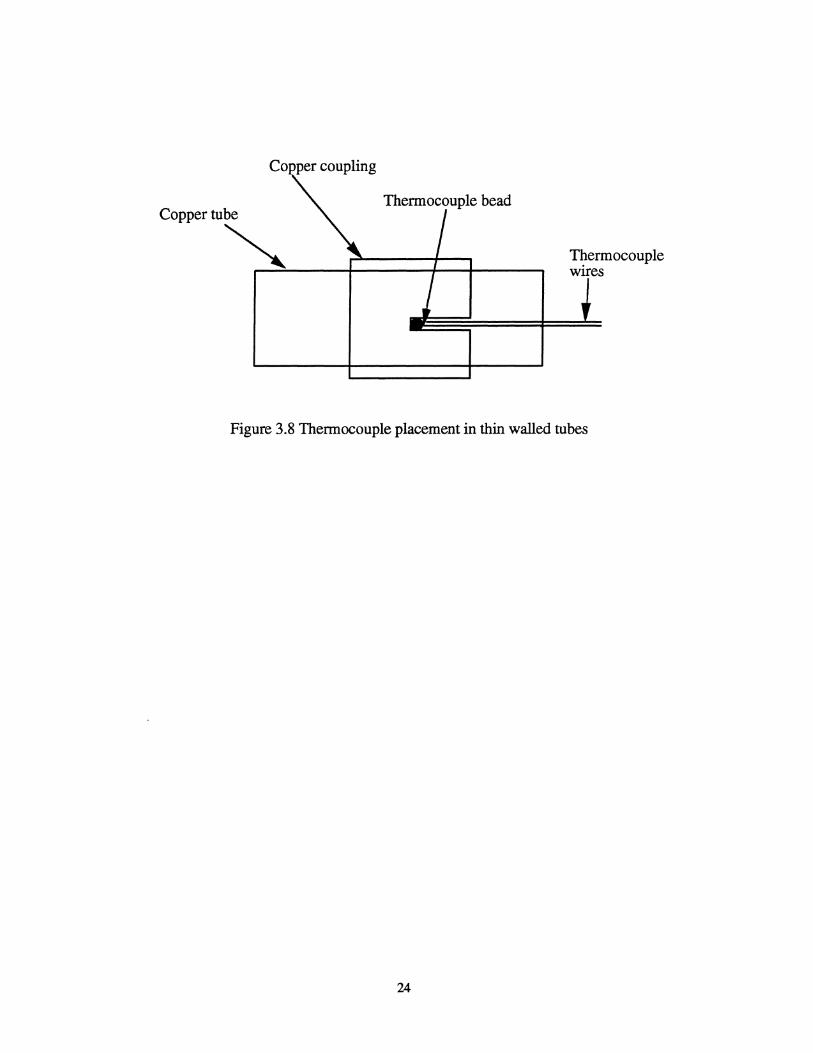
Thermocouple bead
copperru~~~ ____ ~~ ______ ~ __ +-____ ~ Thermocouple wires
Figure 3.8 Thermocouple placement in thin walled tubes
24

Chapter 4
Experimental Procedure and Data Reduction
This chapter discusses the methods to find the test section volume, properly
condition the system to the desired state, and to take a sample to determine the test
section void fraction. One of the key tools not yet introduced is the use of a receiving
tank. The receiving tank is an approximately 1 liter tank with an attached pressure tap and
fittings to connect to the void fraction tap. Graham [1998] developed the void fraction
determination technique and gives an additional description of the method.
4.1- Test Section Volumes
The first task is to find the volume of the test section. This is done by first
evacuating the refrigerant loop then closing all of the valves to the test section. Next one
of the receiving tanks is filled with an known gas usually R134a vapor, R22 vapor, or
nitrogen. The receiving tank is then weighed to find the total mass of tank plus the vapor
in the tank (ml). The tank is then attached to the test section, and the vapor is allowed to
flow freely from the receiving tank into the test section. Mter letting the system
equilibrate, the pressure of the system (P) is recorded from the pressure gage attached to
the receiver, and the ambient temperature (T) is recorded. The receiving tank is now
detached from the system and weighed again (m2). From the two scale readings the mass
released into the test section can be determined (Am) and the specific volume of the vapor
can be found. This test is usually done up to a dozen times with three different fluids and
an average taken as sample calculations appear below.
Am= m1 -m2
v = f(P,T)
'V ts = Am*v
25
(4.1)
(4.2)
(4.3)

where f can be the ideal gas law or other property data such as Refprop or EES.
4.2- Void Fraction Calculations
The system is conditioned to desired inlet conditions to begin sample collection.
First the mass flux is set, and then the overall system temperature is lowered by the chiller.
Once the inlet temperature is much lower than 5°C, the pre-heater is used to establish the
desired inlet quality. When the quality and mass flux are set, the false load heater (FLH) is
turned on until a steady state inlet temperature of 5°C is reached. The mass flux and
quality may need to be slightly adjusted as the inlet temperature changes.
After the refrigerant loop reaches steady state, the four-bar mechanism that
controls the test section valves is closed and the bypass loop is opened. An evacuated
receiver is weighed (lIle) and attached to the test section. The void fraction tap valve is
then opened allowing refrigerant to flow into the receiver. The receiver is kept in an ice
bath to keep the pressure inside the receiver low. The test section heaters are turned on to
evaporate any liquid left in the test section. When it is believed that all of the liquid has
been evaporated, the receiver is taken off of the test section and weighed. The pressure of
the system (from the gage on the receiving tank) and the estimated temperature in the test
section (from the thermocouples outside of the test section) are recorded. The amount of
mass in the receiver and the specific volume of the refrigerant left in the test section allow
the void fraction to be found.
Calculation of the void fraction requires knowing the amount of mass trapped in
the test section when the test section shut off valves are closed. First, the mass in the
receiver (111r) is calculated by subtracting the final scale reading mass (mf) from the
evacuated receiving tank mass (me).
(4.4)
26
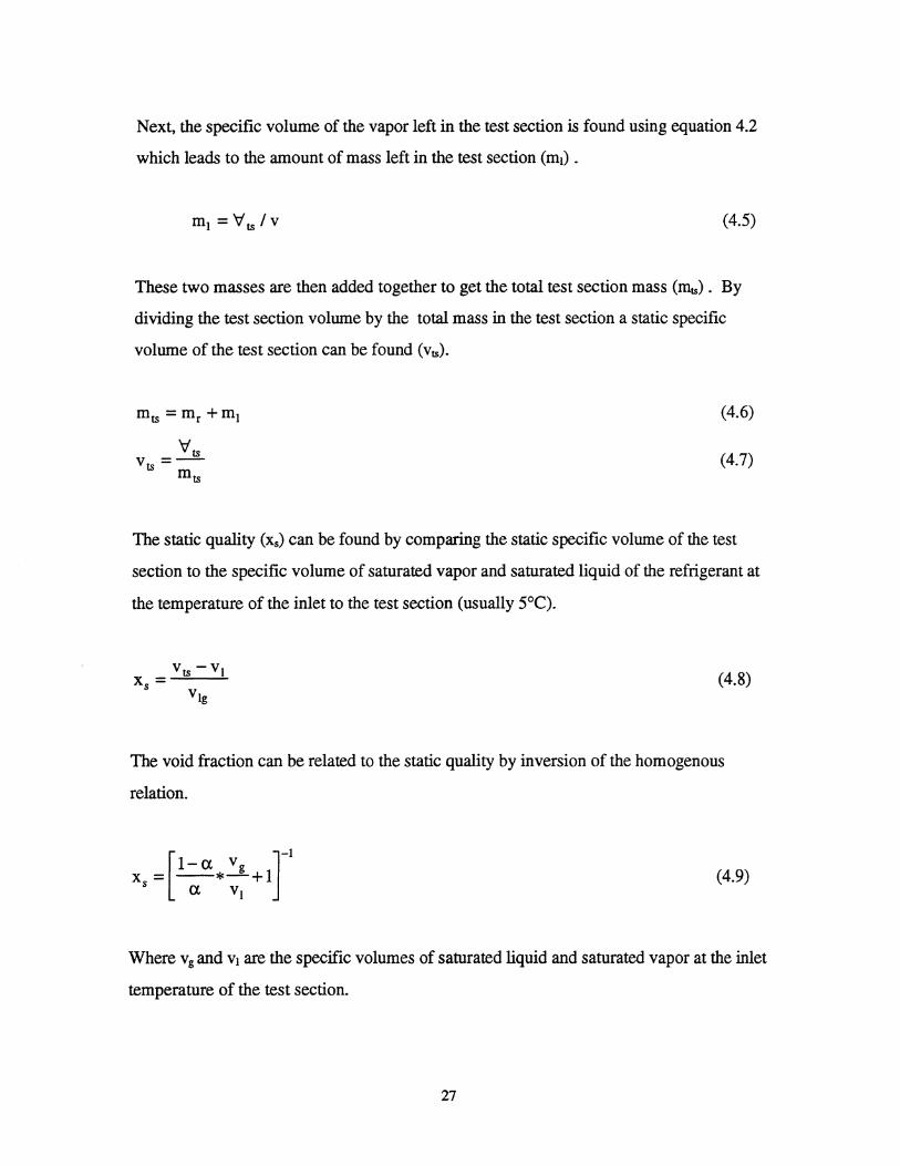
Next, the specific volume of the vapor left in the test section is found using equation 4.2
which leads to the amount of mass left in the test section (ml) .
(4.5)
These two masses are then added together to get the total test section mass (mts). By
dividing the test section volume by the total mass in the test section a static specific
volume of the test section can be found (Vts).
":Its v =
ts m ts
(4.6)
(4.7)
The static quality (xs) can be found by comparing the static specific volume of the test
section to the specific volume of saturated vapor and saturated liquid of the refrigerant at
the temperature of the inlet to the test section (usually 5°C).
(4.8)
The void fraction can be related to the static quality by inversion of the homogenous
relation.
[ ]-1
I-a Vg x = --*-+1
S a v I
(4.9)
Where v g and VI are the specific volumes of saturated liquid and saturated vapor at the inlet
temperature of the test section.
27

4.3- Uncertainty Analysis
Table 4.1 is a table of the average quality of test section and the uncertainty
associated with void fraction measurements at that quality for that tube.
Table 4.1 Void fraction uncertainty for given quality range and tube
Quality Range Smooth Axially Grooved Helically Grooved 0-10% 5.0% 5.0% 3.2% 10-20% 4.8% 2.4% 2.0% 20-30% 2.0% 1.3% 1.6% 30-40% 1.5% 1.2% 1.3% 40-50% 1.4% 1.1% 1.0% 50-60% 1.0% 1.0% 0.7% 60-70% 0.8% 0.9% 0.6% 70-80% 0.7% 0.8% 0.4%
80-100% 0.6% 0.7% 0.3%
This table was constructed by plotting the average uncertainty for each data point, then
using a hand drawn curve which would be higher than 95% of the errors, (see Figure 4.1).
As quality increases error decreases. This is expected since the highest mass
measurements were in the low quality range leaving more room for error.
28

4.00 , ,
--------------~---------------~---~ .... ~~ ............ ~~~ , , , , , , o D=7.26mm R134a ,
3.00
, . : o D=7.26mmR410A • D=8.89mm R134a
o : • D=8.89mm R410A , , ,
2.00
1.00
.- - --.-!- -- - --~-- - -- - ----- -./=.; --------- --- --:----- -- --- - --- --:- --- -- --- --- --~ I ~ I • 0: : : : ,..p., 0., 0' , - I I I I ·.0:0 : ..: :
• • I I I
- --~--~.;;---~~--~-------------:---------------:-::----------OlD' ,
0.00
o 20 40 60 80 100
Average Quality
Figure 4.1 Example error analysis plot for the helically grooved tube.
29

ChapterS
Smooth Tube Experimental Results
This chapter will present and discuss void fraction results for evaporation in a
6.12 mm inner diameter smooth tube. The results to be discussed in this chapter have been
detennined using the equipment and methods discussed in Chapters 3 and 4. The results
will also be compared with existing models. In Chapter 8 all of the void fraction data from
the smooth and enhanced tubes will be presented and a model will be given to predict void
fraction.
5.1- Void Fraction Results
The experimental void fraction results are presented in this section. Void fraction
dependence on refrigerant, mass flux, heat flux, and diameter are discussed.
5.1.1- Effect of Refrigerant on Void Fraction
Figure 5.1 is a plot of measured void fraction for R134a and R410A with respect to
average quality. The plot shows R134a to have a slightly higher void fraction (-5% on
average) than R410A at the same average quality. This was expected because R410A has
a higher vapor pressure and thus higher vapor density causing the vapor to flow at a lower
velocity.
5.1.2- Effect of Mass Flux on Void Fraction
Figure 5.2 plots the measured void fraction with respect to average quality in the test
section at different mass fluxes with R134a as the refrigerant Additionally, Figure 5.3
plots the measured void fraction with respect to average quality in the test section at
different mass fluxes with R410A as the refrigerant The three different experimental mass
30

fluxes are 75 kglm2s, 200 kglm2s, and 500 kglm2s. Figure 5.2 depicts void fraction being
independent of mass flux. Figure 5.3 shows the higher mass fluxes having lower void
fractions at low qualities, but for the most part all of the data points are mixed showing a
trend of mass flux independence. Appendix A contains more detailed plots of the data and
trends discussed here.
5.1.3- Effect of Heat Flux on Void Fraction
Figures 5.4 and 5.5 display plots of void fraction with respect to average quality in
the test section with three different heat fluxes into the test section. Figure 5.4 represents
the void fraction for R134a and Figure 5.5 represents R41OA. The three different heat
fluxes are 0 W/m2 (adiabatic) , 3 W/m2, and 10 W/m2. Both figures show that void fraction
is independent of heat flux. Figures in Appendix A show more detailed plots of the heat
flux effects.
An important point to be brought out is that the aforementioned plots were made
average quality and not inlet quality as the independent variable. The average quality
takes into account the heat flux into the test section. Thus in reality heat flux does bear
some effect on the void fraction.
5.1.4- Effect of Diameter on Void Fraction
. Data was also taken using the same experimental apparatus in a companion study
by Yashar [1998]. His work concentrated on smaller diameter smooth tubes. Yashar's
data for a 4.26 mm inner diameter tuber is plotted with the 6.12 mm smooth tube data and
appears in Figure 5.6. No size trends are seen in this plot indicating that void fraction has
no dependence on diameter within this range of operation.
31

5.2- Correlation Comparison
This section will present and discuss the accuracy of the void fraction correlations
presented in Chapter 2 with respect to the 6.12 mm inner diameter smooth tube data.
Each of the figures is enhanced to show any mass flux dependencies or refrigerant
dependencies of the correlation.
5.2.1- Slip Ratio Correlations
The experimental data is plotted against the Homogenous, Rigot, Zivi , Ahrens
Thorn, and Smith correlations in Figures 5.7 - 5.11, respectively. The Ahrens-Thorn,
Rigot, and Zivi plots are very similar to the Homogenous plot except they are rotated
upward about the pure vapor point. These correlations over-predict the void fraction at
high qualities, but then the correlations swing and under-predict the void fraction at lower
qualities. The Smith correlation does a good job of predicting void fractions above 0.70.
Below a void fraction of 0.70, the Smith correlation also starts to swing upward like the
other slip-ratio correlations. No mass flux or refrigerant preferences were seen in any of
the correlations.
The Homogenous correlation drastically over-predicts the void fraction by up to
38%; on average it is 10.2% in error. The Rigot correlation also over predicts the void
fraction until it's swing point at a void fraction of about 0.75. The Rigot correlation will
predict the void fraction within 12.3% with an average deviation of 5.2% from the
experimental data. Zivi' s correlation is extremely accurate for void fractions of 0.80, but
errors up to 50% for void fractions lower than 0.55. Zivi's correlation deviates from the
experimental void fraction by an average of 4.5%. The Ahrens-Thorn correlation predicts
the void fraction to within 15% with an average deviation of 4.5%. The Smith correlation
is extremely accurate for void fractions above 0.70, predicting the void fraction within
4.5% with an average deviation of 1.5%. Smith's correlation correctly predicts all of the
larger smooth tube data within 14% with an average deviation of 2.2%.
32
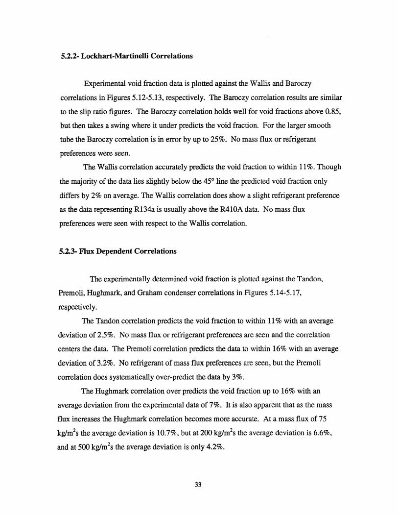
5.2.2- Lockhart-Martinelli Correlations
Experimental void fraction data is plotted against the Wallis and Baroczy
correlations in Figures 5.12-5.13, respectively. The Baroczy correlation results are similar
to the slip ratio figures. The Baroczy correlation holds well for void fractions above 0.85,
but then takes a swing where it under predicts the void fraction. For the larger smooth
tube the Baroczy correlation is in error by up to 25%. No mass flux or refrigerant
preferences were seen.
The Wallis correlation accurately predicts the void fraction to within 11%. Though
the majority of the data lies slightly below the 45° line the predicted void fraction only
differs by 2% on average. The Wallis correlation does show a slight refrigerant preference
as the data representing R134a is usually above the R410A data. No mass flux
preferences were seen with respect to the Wallis correlation.
5.2.3- Flux Dependent Correlations
The experimentally determined void fraction is plotted against the Tandon,
Premoli, Hughmark, and Graham condenser correlations in Figures 5.14-5.17,
respectively.
The Tandon correlation predicts the void fraction to within 11 % with an average
deviation of 2.5%. No mass flux or refrigerant preferences are seen and the correlation
cen~rs the data. The Premoli correlation predicts the data to within 16% with an average
deviation of 3.2%. No refrigerant of mass flux preferences are seen, but the Premoli
correlation does systematically over-predict the data by 3%.
The Hughmark correlation over predicts the void fraction up to 16% with an
average deviation from the experimental data of7%. It is also apparent that as the mass
flux increases the Hugbmark correlation becomes more accurate. At a mass flux of 75
kg/m2s the average deviation is 10.7%, but at 200 kg/m2s the average deviation is 6.6%,
and at 500 kg/m2s the average deviation is only 4.2%.
33

Graham's correlation does not represent the data well. This correlation has a
strong mass flux dependence, and the plot shows how insensitive the void fraction data is
to mass flux. For mass flux's of 500 kglm2s, Graham's correlation does a fair job of
predicting the void fraction with a maximum deviation of 11 %. For the lower mass fluxes,
Graham's correlation over predicts the void fraction by up to 29%.
5.2.4- Diameter Effects on the Correlations
Appendix A contains detailed figures which depict the correlations with both the
4.26 mm and 6.12 mm inner diameter smooth tubes. The data does not show significant
diameter effects, except for the Tandon correlation. The Tandon correlation depicts void
fractions in smaller tubes being higher than for larger tubes.
34

c o .-..... ~
d:: '0 .-o >
1
0.4
0.2
o o
. . . : DO: 0: : : CT ~ .: :
..... <{)-0 .06 ...... t' .~. L ............. 1. .............. j ............. . ; 0 •• : : : : \ . . . .
I I I I I I I t I I • I
~ . . . · . . · . . · . .
I I I I
-------------~---------------T---------------r---------------~-------------.'
· · ·
20 40 60
Average Quality
o R134a • R410A
80 100
Figure 5.1 Void fraction vs. average quality 6.12 mm inner diameter smooth tube.
c o .-..... e ~ '0 . -o >
1
0.8
0.6
0.4
0.2
o o
· · 0: I. ox . S(x 0: . .
-_ .. --~. -c::lX.. ...................... -- .. ~ ..... -_ .. -- .......... -.. -:- .. -- .... -.. -_ .. -_ .. --:- -- .................... .. ~x l ~ ~ ~ · . . · . . · . . · . . · . . · . .
-------------~---------------~---------------y---------------T-------------
· . . ............................ t"' ............................ -~ ............................ -,- ............................ -,- ........................ ..
20 40 60 Average Quality
o G=75
x G=2oo
• G=5oo
80 100
Figure 5.2 Void fraction vs. average quality using R134a in 6.12 mm inner diameter smooth tube. Mass flux (G) given in kglm2s.
35
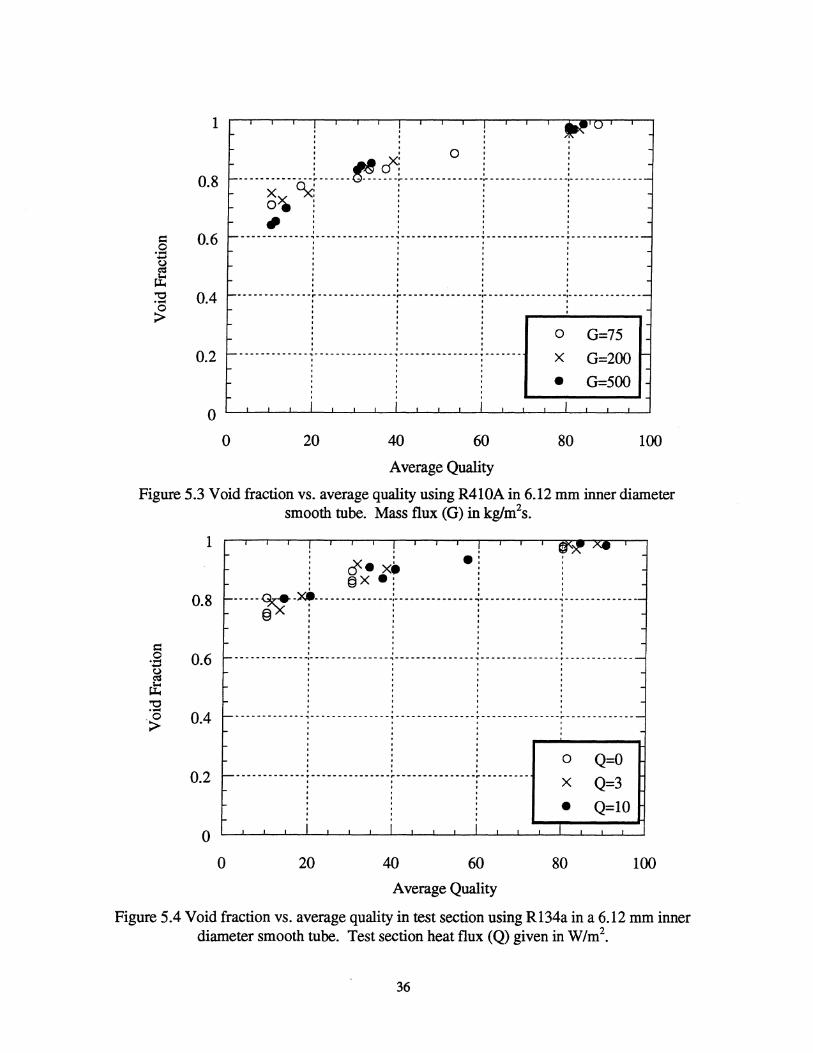
s:: o ..... .... ~ tt '0 ..... ~
1
0.8
flO I I
--------------~ ------~ -?~ ---------------1- ---------------1- -------------0.. I I I
Xx -x: : : : 0-. : : : : ~: : : :
0.6 I , I I
.. -----------,---------------~---------------~---------------y-------------I I I I I I I I I , I I
I • I I
I • I I , , , , , , , , , , , ,
0.4 I , • I
.............................. I'" .............................. -'-" ........................... -,- ............................. -,- ........................ ..
o G=75 0.2 X G=2oo
, , -------------,---------------,---------------y-------
- G=5oo o ~~~~~~~~~--~~~~~~~~~~~~
o 20 40 60 80 100
Average Quality
Figure 5.3 Void fraction vs. average quality using R410A in 6.12 mm inner diameter smooth tube. Mass flux (G) in kglm2s.
s:: o • .::;1
~ '0
.~
1 , , c3<- ~ _:
, §x -: , , 0.8 --- --~ -~-- --- --- --- ----1-- ------- ----- -+ --- --- --------~- -- -----------
§: : : ;
0.6
0.4
0.2
o o
I I I I
-------------,---------------T---------------r-------- -------r-------------t I I I
t I I I
I • I I
: : ~---------, , , , , , , -------------r---------------r---------------~-------- ..
20 40 60
Average Quality
o X
Q=O
Q=3
- Q=lO
80 100
Figure 5.4 Void fraction vs. average quality in test section using R134a in a 6.12 mm inner diameter smooth tube. Test section heat flux (Q) given in W/m2•
36

d o .... ... ~ "0 .... o >
1
0.8
0.6
0.4
0.2
o o
,
, .' : ~.J': : : -----~ ~--~f --------------f ---------------f -------" -------i- -------------
0-. : : : : e<: : : :
f I I I
--.----------,---------------.---------------~---------------T-------------I I I I I I I I I • I I , I I I
I I I I
, " , " , " , " I I I I
................................ r ................. "''' ................................................................................................ -,- ................................ .. I I I I I • I I
I I I I
:: ~~------~ , , , ,
20 40 60
Average Quality
o x
Q=O
Q=3
• Q=lO
80 100
Figure 5.5 Void fraction vs. average quality using R410A in a 6.12 mm inner diameter smooth tube. Test section heat flux (Q) given in W/m2•
d o .... ... ~ "0 .... o >
1
0.8
0.6
0.4
0.2
o
, , , : M: 0·: , , "- ' , O : 0 ~'D .: : I I • •
-~--PC-D---- --- ----1--- --- --- -- --- -1- ------------ --1--- --- ---- -- --I • I I
O I I • •
• I I I I I I I I I I I
I I I I -B--- .. -_ .. _ ....... !- -- .......... - ..... -- ..... -~ .. - ......... -_ ...... -_ ...... ~-- --- --- ................ ~- ....................... .. I • , I
I I I I , , , , , ,
, , o D=4.26mm Rl34a -------------~---------------T---------------, , , , , , , , o D=4.26mm R410A
, , , , , , , , • D=6.12mm Rl34a , , , , • D=6.12 mm R410A -------------T---------------r--------------, , , , , , , , ,
20 40 60 80 100
Average Quality
Figure 5.6 Void fraction vs. average quality for a 4.26mm and 6.12mm inner diameter smooth tube using R134a and R41OA.
37

I
0.95
0.9 o G=2ooR134a : : : : 0 0
: ! I : ~ <> G=5oo Rl34a ----:----------:---------: --------T--o~-
c:: 0 0.85 .... .... ~ tt 0.8 "0 .... 0 > 0.75
: :~~R:!~~A ... -j-.. __ .... ;-...... --f ... -.. elf. • G=5oo R410A ---; ---------!-------o-~--~ --;--------
, I I : : _: :
, , I • I I 0 I
-------i---------1---------;-------~---------f------~t---------t-------: : : :. : : :
0.7 : : : .: : : : .................... ~ ..................... , .................... ~ ................... -:- ............. -.:- .................. --:- ................ -:- .............. ... • , I I I I
I I I. I I I I I I I I ,
0.65
0.6 0.6 0.65 0.7 0.75 0.8 0.85 0.9 0.95 I
Homogenous Correlation
Figure 5.7 Void fraction vs. Homogenous correlation for 6.12mm inner diameter smooth tube using RI34a and R410A Mass flux (G) is in kglm2s.
I
0.95
0.9
0 G=75 Rl34a 0 G=2ooR134a
<> G=5OOR134a : : : <>: 0
------1- -------- -1- -------- ~- ------0 !-CP:J- ----c:: 0 0.85 .... .... ~ tt 0.8 "0 ....
• G=75R41OA
• G=2ooR410A
• G=5OOR41OA
-- --- -J- --- --- --: --- ---11-+-- -~--£ff -----: : I _. : : : Oh : , , , -----: --o----~-~--·--r--------~--------
0 .> 0.75
I , I I I I I
-------~ -. ------~ ---------~ --------~ ------~ ---------r ---------~ -------: :. : : : : :
0.7 :. : : : : : :
.................... ~................ I ............... -~ ................... -:- .................... -;- ................... -:- ................. -:- .............. ..
I I I • I I I
• I I I I I •
I I I • I I I
0.65
0.6
0.6 0.65 0.7 0.75 0.8 0.85 0.9 0.95 I
Rigot Correlation
Figure 5.8 Void fraction vs. Rigot correlation for 6.12mm inner diameter smooth tube using R134a and R410A Mass flux (G) is in kglm2s.
38

I
0.9
d 0.8 o . .= ~ ~ ~ 0.7 .-o >
0.6
0.5
0.5
: : : 0 ......................................... ~ ............................................ ~ .................................... -:-............................. ... I ~ ...................... ..
1 1 1 aqO : : : -: · .
·············1·········~·;.<>i·····~······ :. ···········f·············
• 8 i. o . • ~: 0 G=75 R134a
.............. : ..•.......... : ............... 0 0=200 R134a · . · . · . : : · . · .
0.6 0.7 0.8
Zivi Correlation
<>
• G=500R134a G=75R41OA
• G=200R410A • G=500 R410A
0.9 I
Figure 5.9 Void fraction vs. Zivi correlation for 6.12mrn inner diameter smooth tube using R134a and R410A Mass flux (G) is in kglrn2s.
I
0.95
0.9 d 0
0.85 . .= ~ ~
0.8 ~ .-0 .>
0.75
0.7
0.65
0.6
0.6
G=200 RI34a : : . . 0 : : : <><>: <> G=500 R134a ...... : .......... : ............. ··o··An .... . : : : :.
: ~~~:!~~A ...... J ......... : ....... ~ .. ~EPf- ..... . • G=500 R410A .. .Q.! ....... J. ..... g!1 .. ~ ..... L ..... . : : : .:<> : : : : : : : 0: : :
-------~----II---~- ... -------,------~-!-II------!---------~---------~-------I • I 0 I I • I I • I I I I I
• I I I , I
: • I , I I I I
............................................ : ......................................... -~ ....................... -;_ ..................... ~- ...................... ~ ................... .. • I I I , I
I I f I I I
I I I I I I
0.65 0.7 0.75 0.8
Ahrens-Thorn
.
0.85 0.9 0.95 I
Figure 5.10 Void fraction vs. Ahrens-Thorn correlation for 6.12mm inner diameter smooth tube using RI34a and R41OA. Mass flux (G) is in kglrn2s.
39

§ '':= ~ r.t -e .... o >
1
0.95
0.9
0.85
0.8
0.75
0.7
0.65
-------i---------t---------r---------r------dO : . -- --8- -:- -- ------ -:-- ---- --
I I I , I I I ,
I I I I . .
0: : ........ -.-:- --- ......... -~--- .. -_.. .. .. - .. -_ ... -~- .. -- --_ ..... ~ .. · .. · .. · .. _____ ~1 .. _______ : ________ £ .. ________ : _________ ~_
I I I I I I' I , •• I
I I. I I I' I .
0
0
<>
• • •
· · · · G=75 R134a G=200R134a G=500R134a
G=75R41OA
G=200R41OA G=500R41OA
0.6 ~~~~~~~~~~~~~~~~~~~~~~
0.6 0.65 0.7 0.75 0.8 0.85 0.9 0.95 1
Smith Correlation
Figure 5.11 Void fraction vs_ Smith correlation for 6.12mm inner diameter smooth tube using R134a and R410A Mass flux (G) is in kglm2s.
1
0.95
0.9
s:: 0.85 0 • .:= ~ r.t 0.8 -e .... 0 > 0.75
. . D-' . _ ... ______ : _____ ........... ~-... ---- I ____ -=-~- .. _ ...... -..... ~ ..... --
I I I I
0 G=75 R134a 0 G=200R134a
,. I I
I' • I I I I • I <> G=500R134a I I I I •
0.7 -------~---------I----- .. ---~--------:---------~----•• I I • G=75R41OA I I I I I I I I . .. • G=200R41OA
0.65 • G=500R41OA
0.6
0.6 0_65 0.7 0.75 0.8 0.85 0.9 0_95 1
Wallis Correlation Figure 5.12 Void fraction vs. Wallis correlation for 6.12mm inner diameter smooth tube
using R134a and R410A Mass flux (G) is in kglm2s.
40

1
0.95
0.9
s:: 0.85 0 .............. -:- ..................... : .................. .. · . • :;2
~ 0.8 tt
"t::) .... 0
0.75 >
0 G=75 R134a 0 G=200R134a
<> G=500R134a
· . · . · . : : : 0 I ................ ~ ............ -0 _I. ............ _()-!_................ ,_ .......... .. . ~ . . : • I ! : : I 0: : --------:- --- --~. -------. -- --- --- -~- -----I 0 I I I _
• I • I
• I • I .. . 0.7 • G=75R41OA
0.65 - G=200R41OA
• G=500R41OA
0.6 0.65 0.7 0.75 0.8 0.85 0.9 0.95 1
Baroczy Correlation
Figure 5.13 Void fraction vs. Baroczy correlation for 6. 12mm inner diameter smooth tube using R134a and R41OA. Mass flux (G) is in kglm2s.
1
0.95
0.9
s:: 0.85 0 .... -~
tt 0.8 "t::) .... 0
'> 0.75
0.7
0.65
0.6
0.6
I I I I I --------r-------- .. r--- .... -.... ~ .... -- .... ---~- .... --- ...... , ...... -- .. I I I • t I I • ,. •
: : : : : <'...M>: : ----- --or --- -- -- -T- --- ----T --- -----r--------•• ~_--...;--1_--_--_-_--_--..;..! -_--_--_-_-""'-_
................. ~ ................ -~ .... .O- .......... -~- ................. '.. .. .... Ji .. ~ ....... .. • • I <> I ,
: : . : :
-- ---- -Of -- --- --+- -------;~- ~-+--------1-- --I I I • •
:.: : : : ....... -- -- .. ~ --- _ .... _ .. ,--'" - ... -- .... -:.-_ ..... _ .. --:--_ .. - ..... -- ~ .. -.... · . . · . · .
o o <>
• •
G=75 R134a
G=200R134a
G=500R134a
G=75R41OA
G=200R41OA
• G=500R41OA
0.65 0.7 0.75 0.8 0.85 0.9 0.95 1
Tandon Correlation
Figure 5.14 Void fraction vs. Tandon correlation for 6.12mm inner diameter smooth tube using R134a and R41OA. Mass flux (G) is in kglm2s.
41

1
0.95
0.9
= 0.85 0 .,p
~ tt 0.8 't:I .... 0 > 0.75
, 0 -------1---------~---------1---------7------4( --------i---------t-------
: : : :e : : : , I I I • I I
I I I 0' '.r--' ___ ' __ ...... --, ......... -_ .. --~- .... -.. o--~- ..... ---- --~ .. ---~ . -- --- _ .. --: .. _ ..... 1 • ? 1 1
---lIJ-~---------;------ ' .. ________ 1 _________ ; ___ _ "0 :: : . : " ,
0 G=75 R134a 0 G=200R134a <> G=500R134a
I I I , I 0.7 .............. --: ............. -_ ... : ........ _ .... -: .. _ .......... --: ................. -:- .... ... • G=75R41OA , I , I I
I I t I I , • G=200R41OA 0.65 • G=500R41OA
O. 6 ~..L...L..J.-L...J.-1--L...JL.......L....L.-L....L.-L...L...L..J.-L....L.....L-'-'--L...JL.......L....L.-L....L.-L...J.-L...L...L....L...JL.......L...~J-.J
0.6 0.65 0.7 0.75 0.8 0.85 0.9 0.95 1
Premoli Correlation
Figure 5.15 Void fraction vs. Premoli correlation for 6. 12mm inner diameter smooth tube using R134a and R410A Mass flux (G) is in kglm2s.
1
0.9
0.8
0.7
0.6
0.5
• • • ••••••••••••• ~r ••••••••••••
,
, ---_ ....... _--- ..... --. , , , , , , , .
--------------.---------------~
0.6 0.7 0.8
Hughmark Correlation
0 G=75 R134a 0 G=200R134a <> G=500R134a
• G=75R41OA
• G=200R410A
• G=500R410A
0.9 1
Figure 5.16 Void fraction vs. Hugbmark correlation for 6. 12mm inner diameter smooth tube using R134a and R410A Mass flux (G) is in kglm2s.
42

1
0.9
s:: 0.8 0 .,:1
~ ~ 0.7 ~ .... 0 >
0.6
0.5
0.4
0.4
? 0 • , t I • Q I -----------i ------------i-------------t -----~ ----:t:lI-. -0-0 • f ----------: : • : I
I . I I.'
, '.' 1IIiJ' , -----------:- ------------~ ---_.- ------ ' ------------.--~ --------:- ----------: : : 0 :0,------'---""""---, : : : . , , ,
, , '.' ................ --_ ... , .. -____ ------ ,-- ..... _------_ ... :............ ....- .. ~ .... ~ ; p , , , , , , ,
0.5 0.6 0.7 0.8 Graham Correlation
o
o <>
G=75 R134a
G=200R134a
G=500R134a
• G=75R41OA
• G=200 R410A
• G=500 R410A
0.9 1
Figure 5.17 Void fraction vs. Graham's condenser correlation for 6.12mm inner diameter smooth tube using R134a and R410A Mass flux (G) is in kglm2s.
43

Chapter 6
Axially Grooved Experimental Results
This chapter provides the void fraction results for experimentation on a 8.93 mm
base diameter axially grooved tube for R134a and R410A The characteristics of the tube
and experimental setup were discussed in Chapters 3 and 4. The results will also be
compared with existing void fraction models. In Chapter 8 a model to determine void
fractions in smooth, axially grooved, and helically grooved tubes will be presented.
6.1- Void Fraction Results
The experimentally determined void fraction will be presented and the effects of
refrigerant, mass flux, heat flux, diameter, and internal grooves on void fraction will be
discussed.
6.1.1- Effect of Refrigerant on Void Fraction
Figure 6.1 is a plot of measured void fraction for both R134a and R410A with
respect to the average quality in the test section. The plot shows that the void fraction for
R134a tends to be slightly higher (-7%) than the void fraction for R410A at the same
qUality. This was the expected trend because R410A has the higher vapor pressure and
therefore a higher vapor density causing the vapor to flow at a lower velocity.
6.1.2- Effect of Mass Flux on Void Fraction
Figures 6.2 and 6.3 are plots of void fraction vs. average quality for Rl34a and
R41OA, respectively. The mass fluxes used are 75 kglm2s, 200 kglm2s, and 500 kglm2s.
Each figure shows a slight mass flux dependence as higher mass fluxes give higher void
44

fractions for the same average quality. Appendix B contains additional figures of more
detailed plots showing the effects of mass flux.
6.1.3- Effect of Heat Flux on Void Fraction
The effect of heat flux on the test section is depicted in Figures 6.4 and 6.5 for
both R134a and R4IOA, respectively. Each figure plots void fraction against average
quality and contrasts heat fluxes of 0 W/m2, 3 W/m2, and 10 W/m2. Both figures indicate
that void fraction is independent of heat flux. Figures in Appendix B are of more detailed
plots showing the effects of heat flux.
It is important to note here, as in the last chapter, that the above mentioned plots
are made against average quality and not inlet qUality. In calculating the average quality
the test section heat flux must be taken into account
6.1.4- Effect of Diameter on Void Fraction
A companion study by Yashar [1998] was done on the same experimental
apparatus using a 7.25 mm base diameter axially grooved tube. Figure 6.6 is a plot of
void fraction vs. average quality for the axially grooved tubes distinguishing the two
different diameters. A slight deviation appears between the two diameters. For axially
grooved tubes larger diameters tends toward higher void fractions.
6.1.5- Effect of Micro-fins on Void Fraction
Figure 6.7 is a plot of void fraction vs. average quality for the 6.12 mm inner
diameter smooth tube and 8.93 inner diameter axially grooved tube. In the axially
grooved tube the void fractions appear to be slightly less (1-2%) at the same average
qUality. This suggests that enhancing the tube lowers the void fraction.
45

6.2- Correlation Comparison
This section will discuss the accuracy of the correlations for the axially grooved
tube data. The only correlations that will be compared are the ones that performed
reasonably well for the smooth tube data which are the Smith, Wallis, Tandon, and
Premoli correlations. The correlations not discussed here are presented in graphical foon
in Appendix B.
Figure 6.8 is a plot of void fraction versus the Smith correlation for the 8.89 mm
inner diameter axially grooved tube. The Smith correlation predicts the void fraction
within 7.3% with an average deviation of 2.4% with the experimental data. Looking
closer at the Smith correlation a mass flux preference appears as the data is layered by
mass flux. At a mass flux of 500 kg/m2s, the Smith correlation under predicts the void
fraction, but at the lower mass flow rates the Smith correlation over predicts the void
fraction. The Smith correlation does an excellent job of centering the data giving no
preference of over predicting or under predicting the void fraction.
The accuracy of the Wallis correlation appears in Figure 6.9. The experimental
void fraction is accurately predicted to within 14.3% within an average deviation from the
Wallis correlation of 3.4%. The majority of the data points lie below the 45° line
indicating the Wallis correlation over predicts the void fraction. A mass flux preference is
also depicted as the data points for the 500 kg/m2s mass flux lie above the lower mass flux
data 'points.
A plot showing the accuracy of the Tandon correlation appears in Figure 6.10.
The Tandon correlation is accurate to within 7.8% with an average deviation of 2.3%
from the experimental data. The data is centered and no mass flux preference is seen, but
a refrigerant preference is depicted. The data points for the R134a data lie above the data
points for the R410A data.
Figure 6.11 is a plot of the experimental void fraction against the Premoli
correlation. The Premoli correlation is accurate to 5.6% with an average deviation of
46

1.9% to the experimental data. The Premoli correlation centers the data well and shows
no preference to mass flux or refrigerant
Figure 6.12 through Figure 6.15 are plots of void fraction with respect to the
Smith, Wallis, Tandon, and Premoli correlations, respectively. Yashar' s data was added
to these figures to display the effect of diameter on each correlation. These figures
indicate no dependence on diameter for any of the correlations.
47

s:: o ..... ..... g tt "0 ..... o >
1
0.8
0.6
0.4
0.2
o o
· . . : f. : 0 : ~ c9~. i ~ OrC"\ : , : : : -----'& -; -f _.- -. - -------:----------------:- ---------------:- -------------
,. i : -------------~---------------~---------------T-------- -------T-------------I I I I
I I • I I • I ,
I • I I I • • I · .. · .. · .. . . I I • I
.............................. r .......................... .... -r- ............................................................... -,- ........................... -· . · . · . · . · . · , · . · . , , · . o R134a • R410A
20 40 60 80 100
Average Quality
Figure 6.1 Void fraction vs. average quality for a 8.89 mm base diameter axially grooved tube.
s:: o .,:::
~ "0 ..... ~
1
0.8
0.6
0.4
0.2
o o
. @<
· &d<1 o. . .: 0: : : .................. -~ ..................................................................... -,_ ............................... -,- ........................... ..
Ix: : : : §it: ! : :
I • I t .. . • I I I I I I I
-------------~---------------,---------------T-------- -------T-------------I I I I I I I • .. . .. . " . .. . .. . ., . .. . I I I I - .... -- - .. _- --- --po -_ .. -- ---- ...... -_ ...... - ......... - .......... _ ......... - .. - ............... _ ........... _,_ .. - _ ... _ .. -- --_ .. ...
o G=75 · . -------------,---------------.-- .. ··········--T·--- x G=200 --
• G=500
20 40 60 80 100
Average Quality
Figure 6.2 Void fraction vs. average quality using R134a in a 8.89 mm base diameter axially grooved tube. Mass flux (G) given in kglm2s.
48

1
0.8
§ • .:= 0.6
~ "0 ..... o 0.4 >
0.2
o
! , ! , , ! , ,
: : 0: :
1 "cS 1 1 1 -- - ---- ----- ---~ ---0 - t§-':. -----:- ---------------:- --------------~ ---------------X : : : :
~o 1 1 1 1 r-M------------~---------------~---------------~------- --------:---------------
I I I I , , , , , , , , , , , , , , , , , , , , , I • I I
---------------~---------------!---------------~---------------~---------------
: : : ---'---.. , , , , , , , , , , , , , , , ~-------------T---------------r---------------r------, , , , , , , , , , , , , , , , , , , , ,
i i i
o 20 40 60 Average Quality
o x
• i
80
G=75
G=2oo -
G=5oo
100
Figure 6.3 Void fraction vs. average quality using R410A in a 8.89 mm base diameter axially grooved tube. Mass flux (G) given in kglm2s.
c: o • .:= ~ ~ "0 ..... ·0 >
1
0.8
0.6
0.4
0.2
o
,
, e~! ., , .: 0: : :
..................... -~ .. r ............................... '"'.- ................................ ..,- .................................. "t ........................... ...
6S<: : : : o ~ ~ , , , , , , , ,
• • I I -------------,---------------T---------------r---------------r-------------I , I I
I I I I
I I I I
: : ------~ , , , , , , , , , , , ------_ .. -----T---------------r---------------r-------, , , , , , , , , , , , , , , , , , , , , , , ,
20 40 60
Average Quality
o x
•
80
Q=O
Q=3
Q=lO
100
Figure 6.4 Void fraction vs. average quality using R134a in a 8.89 mm base diameter axially grooved tube. Test section heat flux (Q) given in W/m2•
49

= o ..... .... ~ ~ "0 ..... o >
1
0.8
0.6
0.4
0.2
o
, I. I : I x I , I : ,--: : : --- -_ .. -_ ....... -- .. ~---... ..--- ... -.. :-- .... _ .. ---- -_ ... -_ .... :--- -_ ..... --_ ...... -_ .. --:---_ .... --_ .. -_ ..... I I • I
~: 1 1 1 1 ex I I I
-------------,---------------~---------------T---------------~-------------I • • , , I I I , , , , , , , , , , , , , , , , , I I I I .............................. ,. ................................. .- ................................................................ -,- ............................ ... , , , , , , , , , , , , , , , , , , , , , , ,
20 40 60 Average Quality
o
x Q=O
Q=3
- Q=lO
80 100
Figure 6.5 Void fraction vs. average quality using R410A in a 8.89 mm base diameter axially grooved tube. Test section heat flux (Q) given in W/m2•
= o ..... .... ~ "0 ..... ~
1
0.8
0.6
0.4
0.2
o o
: 0 : 0 : 0 , ff' I ' , , I I
:. :0 : : : 0 (]~ : :
...... ~~ .. ~..... . ...... : .. ~ .......... ~ ............... ~ ............. . ¥ '~ 0' , ,
I I I •
CJ ' , , , , , I , • I
1 I I I I I I I
I I I I I I I I ... -0-- -...... --- .. -:- --- -- ............... --~- ..... -_ ......... --- ....... ~ .... -_ .... -- ................ : .... -_ ...... -_ ....... -I I • I , , , , , , , , , , , , o , , , , , ,
-------------,---------------T-----------, , o D=7.25mm R134a , , , , , , , , , , o D=7.25mm R410A , , , , , , , , • D=8.89mm R134a • D=8.89mmR41OA
20 40 60 80 100
Average Quality
Figure 6.6 Void fraction vs. average quality for 8.89 mm and 7.25 mm base diameter axially grooved tube using R134a and R41OA.
50

s:: o .... .....
~ '0 .... o >
1
0.9
0.8
0.7
0.6
0.5
o
I I 0: : ..,: . '
·-------------~------~--()--~---il---------~---------------,--------------
: _ 0: i .' , , , -----~~---ii-ii------~---------------~---------------~-------------
~.d ~ ~ ~ 0: : i ' ,
----- ---~---- --------- --~ ------- --- ---.,: : r: : . : ,
-------------~---------------~-------------
0.2
, , ,
0.4 0.6 Average Quality
o o
• •
R134a Smooth
R410A Smooth
R134a Axially
R410A Axially
0.8 1
Figure 6.7 Void fraction vs. average quality for 6.12 mm inner diameter smooth tube and 8.89 mm base diameter grooved tube using R134a and R41OA.
1
0.95
0.9
s:: 0.85 0 .... ..... ~
0.8 tt '0 .... '0
0.75 > 0.7
0.65
0.6
0.6
, -_ ... -- ...... -r -_ ... -_ ... -- -!-_ ...... - --- ... -: ..... _ ..... -_ ... --: .. -_ ... -_ ... -- -:-- -_ ... -0 ... '- ........................ -:- -_ ... -- ... ...
: : : : : ,0 : : : : : : 0 : I I I I I I
..................... -: ........................... : ........................... : ........................... : ... ... ... ... ... ..... : -................... : ........................... : ...... ............ ...
: : : <>: _;- 0: ! I I I • I I I ......... -_ ... --: -_ .. -- ......... -;-_ ... -_ ... -_ ... -;_ ... -_ ... --- ... : .. '" --1- -:-_ ... -_ ... -_ ..... 1_ ... -- ............... _I. -_ ... -- ......
i i F i i 0 R134aG=75 ... ----- ... .J _________ ~ ____ ........ ...-8-- --- ~ _________ J. ___ ...
: : : : : 0 R134aG=200 I I I •
I " I I I I I I
-_ ... -_ ... --~ -_ ...... -.... : .... --.. .Q~ ... -_ ............ --~ -_ ... -_ ... -- -;----- <> R134aG=500 R41OAG=75 .1+ : ~ : ~ •
• R41OAG=200
• R41OAG=500
0.65 0.7 0.75 0.8 0.85 0.9 0.95 1 Smith Correlation
Figure 6.8 Void fraction vs. Smith correlation for 8.93 mm base diameter axially grooved tube using R134a and R41OA. Mass Flux (G) in kglm2s.
51

1
0.95
0.9
= 0.85 0 . .::: ~ tt 0.8 ~ .... 0
0.75 >
0.7
0.65
0.6
0.6
-------t---------t---------;--------- --------. . <>
· .. _- --:- --- ----- -:- -------· . · . · . I I I I I ............... ___ : ... _ .. ____ ... _:_ ... _______ : ____ .. ___ ... : __ _ ._. ________ ~_ ... _ ...... ___ .. J ... __ ... __ .....
l ~ ~ 0 ~ : 0 R134a G=75 -------r-------r-------: -iil---r--------r--- 0 R134a G=200
<> R134aG=500
• R410AG=75
• R410AG=200
• R410AG=500
0.65 0.7 0.75 0.8 0.85 0.9 0.95 1
Wallis Correlation
Figure 6.9 Void fraction vs. Wallis correlation for 8.93 mm base diameter axially grooved tube using R134a and R41OA. Mass Flux (G) in kglm2s.
1
0.95
0.9
= 0.85 0
''::: ~ 0.8 tt ~
-------1---------1---------~---------7------- -------- ---------t-------I I I I I t I I I I' I
I • '<> I I I
-........ -.. --~---------~-- ... -- .. --~--- .. g ..... : ... -.... _ ... :.. ... : : : , : - : : I <>: : : • I • I I
0 R134aG=75 .... '0 0.75 >
I I I I I
-------~---------~--~ ... --.---------!---------!-fl. I I I • I I I
0 R134aG=200
0.7
. <> R134aG=500
• R410AG=75
0.65 • R41OAG=200
• R410AG=500 0.6
0.6 0.65 0.7 0.75 0.8 0.85 0.9 0.95 1
Tandon Correlation
Figure 6.10 Void fraction vs. Tandon correlation for 8.93 mm base diameter axially tube using R134a and R41OA. Mass Flux (G) in kglm2s.
52

1
0.95
0.9
c 0.85 0 .... ... ~
-------i---------i---------i---------f------- ---------t---------t-------• I I I I I . . . .
~ 0.8 0 R134aG=75 "0 .... 0
0.75 > 0 R134aG=200
.. . 0 R134aG=500
0.7 --------~------~: -r:L----~---------~--------I • • I • R41OAG=75
0.65 :.: : : .-----. ---.- ---~- -- ------ ~ -- ------ -~- --- --- --, , I I
I I I I . . . • R41OAG=200
• R41OAG=500 . . . 0.6
0.6 0.65 0.7 0.75 0.8 0.85 0.9 0.95 1 Premoli Correlation
Figure 6.11 Void fraction vs. Premoli correlation for 8.93 mm base diameter axially tube using R134a and R41OA. Mass Flux (G) in kglm2s.
1
0.9
0.8 c 0 .... ... ~
0.7 ~ "0 .... 0 > 0.6
0.5
0.4
0.4
· . ............ -_ ............ -:- ... -_ ... -_ ... -_ ... -- ~ ----- ------. .., ... -
· · · · · . ................................ ~ ......... -- IT ............ :- ............ -- ............ --:- ............. · . . · . . · . . · . . · . .
0.5 0.6 0.7
Smith Correlation
o D=7.25mm R134a
o D=7.25mm R410A
• D=8.89 mm R134a
0.8 0.9 1
Figure 6.12 Void fraction vs. Smith correlation for 7.25 mm and 8.93 mm base diameter axially grooved tube using R134a and R410A
53

1
0.9 o D=7.25mm R134a
o D=7.25mm R410A
= 0.8 -0 . .:= g ~ 0.7 "0 .... 0 > 0.6 ........ IT""''''' "":- ......................... ~ ......................... ~ .................... .. · . . · . · . · . · . · . .
0.5 ........................ ~ .. a ................... ! ........................... ~- ........................ "':- ................... .. I I I I I I • I
I , I I
I I • I I • , I
0.4
0.4 0.5 0.6 0.7 0.8 0.9 1
Wallis Correlation
Figure 6.13 Void fraction vs. Wallis correlation for 7.25 mm and 8.93 mm base diameter axially grooved tube using R134a and R410A
1
0.9
= 0.8 0 . .:= g ~ "0 .... 0.7 0 . >
0.6
0.5
0.4
0.4
· . .----- .. ------~------------~-------------~---~--: : : _ 0 : : 0: · . . · . . .................... _~ ......................... ~ ............ .. .Sit.. ... ................ ~_ ................... .... _:_ ................... .. t. " " I I · . · . · . · . · . .
0.5
-------------~-----
0.6
· · · ·
0.7
Tandon Correlation
o D=7.25mm R134a
o D=7.25mm R410A
- D=8.89 mm Rl34a
• D=8.89 mm R410A
0.8 0.9 1
Figure 6.14 Void fraction vs. Tandon correlation for 7.25 mm and 8.93 mm base diameter axially grooved tube using R134a and R41OA.
54

1
0.9
c: 0
0.8 • .::1
~ d: 0.7 "0 .... 0 >
0.6
0.5
0.4
0.4
, , , ~ .. ________ ~ ____________ ~ _____________ L______ __ _ ________ ~ __________ _ , , ,----~-I I. I
" , " , " , " , , , , -----------~------------~----------, , , , , , , , , , , , , ,
......... _ .. -_ ..... --!-------n-- I ... ---- ..... - ....... -:----
, , , , , , , , , , , , , ,
o o
•
D=7.25mm R134a
D=7.25mm R410A
D=8.89 mm RI34a
D=8.89 mm R410A
0.5 0.6 0.7 0.8 0.9 1
Premoli Correlation
Figure 6.15 Void fraction vs. Premoli correlation for 7.25 mm and 8.93 mm base diameter axially grooved tube using R134a and R410A
55

Chapter 7
Helically Grooved Tube Results
This chapter will present and discuss void fraction results obtained with a 8.93 mm
base diameter helically grooved tube with an 18° helix angle. These results were found
using the equipment and methodology discussed in chapters 3 and 4 using R134a and
R41OA. Chapter 8 will discuss a void fraction model to correlate all of the smooth and
microfmned tube data.
7.1- Void Fraction Results
This section will present the void fractions experimentally obtained on the helical
tube. The effects of refrigerant, mass flux, heat flux, diameter, and internal geometry will
also be discussed.
7.1.1- Effect of Refrigerant on Void Fraction
Figure 7.1 plots void fraction versus average quality for a 8.93 mm base diameter
helically grooved tube using R134a and R410A. The plots shows R134a having a higher
void fraction (-7%) that R410A at the same quality. This was expected since 410A has a
higher vapor pressure and higher vapor density which allows the vapor to flow slower.
7.1.2- Effect of Mass Flux on Void Fraction
Plots showing the dependence of mass flux on void fraction are show in Figures
7.2 and 7.3 for R134a and R410A respectively. These two figures plot void fraction
against average test section quality while the data points distinguish mass flux. Both
figures show that higher mass fluxes tend to give slightly higher void fractions at the same
quality. Appendix C contains more descriptive plots of the data and trends described here.
56

7.1.3- Effect of Heat Flux on Void Fraction
Figures 7.4 and 7.5 plot void fraction vs. average quality for a 8.93 mm base
diameter helically grooved tube distinguishing different heat fluxes for R134a and R410A
respectively. The heat fluxes generated were 0 W/m2 (adiabatic), 3 W/m2, and 10 W/m2.
Neither figure depicts void fraction being a function of heat flux. Figures in Appendix C
contain more detailed graphs of the trends and data presented in this section.
It is important to note here as well as in previous chapters that all plots are made
against average quality and not inlet qUality. Heat flux does affect the average quality and
thus has an indirect effect on the void fraction.
7.1.4- Effect of Diameter on Void Fraction
Figure 7.6 is a plot of void fraction vs. average quality for 7.25 mm and 8.93 mm
base diameter helically grooved tubes. For R134a near a quality of 30% it appears that the
smaller tube gives a slightly higher void fraction at the same qUality. The rest of the plot
shows void fraction being independent of diameter. It is the author's opinion that Figure
7.6 depicts no influence of diameter on void fraction and the aforementioned specific
points are within experimental error of supporting this claim.
7.1.5- Effects of Tube Enhancements on Void Fraction
Figure 7.7 is a plot comparing the void fraction in the 8.93 mm base diameter
helically grooved tube to the 6.12 mm inner diameter smooth tube. The figure shows the
helically grooved tube giving a slightly lower void fraction at the same quality. Figure 7.8
is a plot comparing the void fractions of the 8.93 mm base diameter helically grooved tube
to the 8.89 mm base diameter axially grooved tube. This figure depicts the helically
grooved tube having a slightly lower void fraction at the same qualities.
57

7.2- Correlation Comparison
This section will discuss the accuracy of the Smith, Wallis, Tandon, and Premoli
correlations for the helically grooved tube. Though the other seven correlations discussed
in the literature are not discussed here graphs of the accuracy for those correlations appear
in Appendix C.
A plot of the measured void fraction vs. the Smith correlation appears in Figure
7.9. The Smith correlation predicts the void fraction to within 9.2% with an average
deviation of 3.25%. The Smith correlation also shows a mass flux preference as the data
points representing higher flow rates are above the data points representing slower flow
rates. The void fraction is under predicted for a mass flux of 500 kglm2s, but over
predicted for slower mass fluxes. The Smith correlation also sees the swing representative
of the slip ratio correlations (see discussion in Chapter 5). Smith over predicts the void
fraction at high qualities, but the curve swings out and begins under predicting the void
fraction.
Figure 7.10 depicts the accuracy of the Wallis correlation. The Wallis correlation
predicts the void fraction to within 11 % with an average deviation of 3.3%. The Wallis
correlation appears to over predict as most of the data lies below the 45° line. The Wallis
correlation also depicts mass flux and refrigerant segregation.
The accuracy of the Tandon correlation appears in Figure 7.11. The Tandon
correlation is accurate within 9.5% with an average deviation of 3.2%. The Tandon
correlation centers the data nicely and no mass flux preference can be seen. A refrigerant
segregation is depicted as the R134a data lies on top of the R410A data.
Figure 7.12 is a plot showing the accuracy of the Premoli correlation. Premoli's
correlation is accurate within 9.1 % with an average deviation from the experimental data
of 2.5%. A slight mass flux dependence is seen at lower void fractions and the data points
depicting R410A do tend to lie below the R134a points. On the whole though the data
does look evenly mixed. Most of the data lies above the 45° line indicating that the
Premoli correlation slightly under predicts the void fraction.
58

Figure 7.13-7.16 are plots of void fraction vs. the Smith, Wallis, Tandon and
Premoli correlation, respectively. These plots distinguish the two different tube diameters
to aid in determining if the correlations have a diameter preference. No diameter
preferences are seen in the four plots.
59

c:: o ';:3
~ ~ "0 .... o >
1 ~~~~~-r~~~~.-~~~~-r~~-'~r-'-' ! ! ! 0 , • • '
: 0 6 0 .: : , a.... ' , 0.8 _.- ---Q)c;- --t~- -- -r-~ -~+----------- ----1- ---- -- ------ ---1- -- --- --- ------
g. • • : : : : o e-. : : : : o I: : : :
O 6 r------------.-~---------------~---------------!---------------!---------------. : : : ; I I • I
I I • I
I I • I I I • I I • • I I • I I I , • ,
0.4 -_ ........................ -t ............................... -r ............................ -~ ................................. ~- ........................... --I I I I I I • I
I I I I
I I I I
: : : ..------, , , o R134a I-
• R410A O 2 ~-------------~---------------~---------------:----.-. : : : , , , , , , , , , , , , ,
o ~~~~i~~~_~I'~~~~i~~~~i~~~~
o 20 40 60 80 100
Average Quality
Figure 7.1 Void fraction vs. average quality for a 8.93 mm base diameter 18° helically grooved tube.
c:: o .... ~ ~ "0 .... o .>
1
0.8
0.6
0.4
0.2
o
! ! !,O ! '0 '
. X 0 : : I ~: : :
1-- - - - - 'tIix ---?~ -------------1- --------------i---------------1- --------------X: : : :
• I I I I
X 0: : : : I I I I
---------------.~---------------~---------------~---------------:---------------I I I I , , , , , , , , , , , , , , I I I I
r--------------~---------------!---------------~---------------~---------------• I , I
I : : ,......--------w , , , , , , , , , , , , , ~--.----------:---------------~---------------~--------, , , , , , , , ,
j
o 20 40 60 Average Quality
o x
• 1
80
G=75 G=2oo G=5oo
100
Figure 7.2 Void fraction vs. average qUality using R134a in a 8.93 mm base diameter 18° helically grooved tube. Mass Flux (G) given in kglm2s.
60

= o .... .... ~ tt '0 .... ~
1
0.8
0.6
0.4
0.2
! ! ! ~x U'
: I 0; : i 4'x 8'f i i --- --- --- --- ---k----- -0- -- --- -:-- --- --- --- --- --;- --- --------- ---;- ----- ------ ---
'.0: : : : X: : : : ~: : : :
I I I I r-" -- ........ -- .. -_ .. ~- .. -_ .. -_ .. --- -_ .. -~ ........ -_ .. -.... -_ .. -- ~ _ .......... -_ ... -- .... - .. ; .... -_ .. -_ .. -_ .. ---I I I I I I I I
I I I I
I I I • It' I I • I I
I I I I I I I I
--_ ........ -_ .. -_ .. --~ -_ .. -- --_ .. -_ ...... -~- .. -_ .. -- ........... ---:- .. -_ ......... -_ .. -_ ... --:- ............ -- .. -----f I I I
: : : ~--------~ o 0 0
• 0 0 o 0 0
o 0 0 · . . o 0 0 ~ .. -_ ........ -- .. -_ .. ~- ... -_ .. -_ .. -- .. -_ .. -~- ....... -_ .. -_ .. -_ .. --! -_ ........ - .....
o 0 0
o 0 0
• 0 0 o 0 0
o 0 0
o • 0
o 20 40 60 Average Quality
o x
•
80
G=75
G=200
G=500
100
Figure 7.3 Void fraction vs. average quality using R410A in a 8.93 mm base diameter 18° helically grooved tube. Mass flux (G) given in kg/m2s_
= o .... .... £ '0 .... o :>
1
0.8
0.6
0.4
0.2
! · o ·
! !. ! x x· 0 •
A 0 :. ~: : : ------~x ---~- --------------~ ---------------;- ---------------;- --------------o 0 0 0 0
o 0 o o 0
• I I I f-- ... -- --- ......... -_ .. ~- .. -_ .......... -_ .. _ .. - -~ .. -_ .. -_ .. -_ .. -_ .. --! -_ .. -_ .. -_ .. -_ ... -- .. ;- .............. - ....... --I I f I I I • •
I I • •
• I • I • I • • I • I I
I I • I I I I , -_ ........ -_ ..... -_ .. --~ -_ .. -_ .. -_ .. _ .... -- -~ ............ -_ .. -- .. -_ ... -:- .. -_ .. -_ .. -_ ... -_ .... -:- ............ -- .. -- .. --I I I I : : : ~~o ______ _
o 0 0
o 0 0 o 0 0
o 0 0
o 0 • o 0 0 r-- ........... - ........ -- .. ~- .. -_ .. -_ ... -- ... -_ .. -~ .. -- .. -_ .. -- .... _ ..... - ~ -- ........... .. o 0 0
o 0 o • o 0 o 0
o 0
o x
•
Q=O
Q=3
Q=lO
-
o ~~~~i~~~_~lo~~~~i~~~~I~~~~
o 20 40 60 80 100
Average Quality
Figure 7.4 Void fraction vs. average quality using R134a in a 8.93 mm base diameter 18° helically grooved tube. Test section heat flux (Q) given in W/m2•
61

1 ~~~~~~~~~~~~~~~~~~~~~~ ! ! ! ~X x' : : e: : : ~~ : :
0.8 _.- ---- -- ------~-- --- -8------ -r---- --- --- -----r---- ----- --- ---;- --- --- --- -- ---cS,- x: : : : x:: : §: : . :
0.6 r--------------~---------------~---------------;---------------;---------------I I • I · . . · . . · . . · . · . · . · . 0.4 -_ ........................... -~ ................................. -~ ................................ ~ ................................ -:- ......................... --
· . · . . 0.2 r--------------~---------------~--------- .. -----~------- ..
. o ~~~~i~~~~i~~~~i~~~~~~~~
o 20 40 60 Average Quality
Figure 7.5 Void fraction vs. average quality using R410A in a 8.93 mm base diameter 18° helically grooved tube. Test section heat flux (Q) given in W/m2•
1
0.8
0.6
! ! !. ,- .' ; COO~~O _; :
e-- ----!IHP ~<f_ --".p --------------~ ---------------~ --------------I r- : : : :
---------------~---------------~---------------!---------------;---------------o : : : :
I I I I I I I I I , I I , , .
0.4 ~--------------~---------------~---------· . 0 D=7.25mm RI34a · . · , · . · , 0 D=7.25mm R410A · . · . 0.2
· . ~-------------~---------------~---------, . • D=8.93mm R134a
· . · . · . - D=8.93mm R410A · . · . , . . ,
i i
o 20 40 60 80 100
Average Quality
Figure 7.6 Void fraction vs. average qUality for 8.93 mm base diameter 18° helically grooved tube using R134a and R41OA.
62

1 , , , ,
0.95
0.9 s:: 0 . .= 0.85 ~ tt ~ 0.8 ..... 0 >
0.75
-------------~---------------~---------------!-.. -----------: : 0: : : 00:· : : .............. ;. ...... o· .... 'f-...........•. : ................ : ............. . : .: 0: :
------------~;;---1!I!lr~--------------1---------------1-------------..... \: ~1······:······t-··············(· -.. ------... ·1-··· --....... .
° --- ' ···--~-i1--··-·--··--·--i·········-··- ° Smooth R134a
0.7
0.65
.• __ ...... L_._._. __ ..... _~............. 0 Smooth R410A • l l • Helical R134a . ' ,
.... ·W·····~···············~··········· -. • Helical R410A , , , ,
0.6
0 0.2 0.4 0.6 0.8 1
Average Quality
Figure 7.7 Void fraction vs. average quality for 8.93 mm base diameter helically grooved tube and 6.12 mm inner diameter smooth tube.
1
0.95
! ! ! !~
~············-~···············~······---·-----f··------.----~------------0.9
s:: 0 . .= 0.85 ~ tt ~ 0.8 ..... 0 >
0.75
0.7
0.65
. cP' , , , '. 0' . , , .' , -- ---- -- -- -- -- -~ -- - -- -G- -----.- ------ - -- - - -:- - -- - -- - -- - -- - - -:- -- - -- - -- - -- ---: Eo . D : : : 0 ' : :
---------------~------- ~--------------t---------------t---------------o~· .: : :
r- ----~~& -r ---0 -1----- -1- ------------ --~ --- ------ --. ---1-' -. -- ------ ---. : ------".f1iir-------------r----------- ° Axial R134a 1--
__ • __ ~---~-------- .. -----~------------- 0 Axial R410A ._ • ~ 1 1 • Helical R134a
--- --- -F---- -;- --- --------- --;- -- --- ------- • Helical R410A --
0.6 0' , iii i
o 0.2 0.4 0.6 0.8 1 Average Quality
Figure 7.8 Void fraction vs. average quality for 8.93 mm base diameter helically grooved tube and 8.89 mm base diameter axially grooved tube.
63

1
0.95
0.9 = 0 .+=1 0.85 ~ tt "0 0.8 .... 0 >
0.75
0.7
0.65
0.6
0.6
, , , ~ , , I I I I 0 I.: :
............ - .. ~ ...... ---- - .. .. ~ ..... -- ... --¢ .. ~ ........ --_ .. I --- --...... :-_ .. --- .......... '_ .. _ .. _ .. _ .... -'- ----- .. -
~ ~ ~ <> ~ • ~ 0 R134a G=75 ........ ---~--- .... ----~ .. -.. ------ ---- .. -- .. -~ .. --- .... -.... ~ , " :. ::
" , :. I I I I I
~' • I I • ----0 .. r- ................ : ............. -0-:---------:-- .... ---- ... -:· I • I , I I I I I I t • I I • I • I I
0.65 0.7 0.75 0.8 0.85
Smith Correlation
o <>
•
R134aG=200
R134aG=500
R410AG=75
• R410A G=200
• R410AG=500
0.9 0.95 1
Figure 7.9 Void fraction vs. Smith correlation for 8.93 mm base diameter 18° helically grooved tube using R134a and R41OA. Mass flux (G) in kglm2s.
1
0.95
0.9
= 0 '+=1 0.85 ~ tt "0 .... 0.8 0 ;>
0.75
0.7
0.65
0.6
0.6
o R134aG=75
o R134a G=200
<>
• RI34aG=500
R41OAG=75 I , I • I •
• R410A G=200 ---_~--------' __ ~---:----------:--------• R4IOAG=500 1 o~.. l l
----- ---1-- ---- --r --- -----f--~--~ 1 -------:-- ----- -r -------1- --- ----: : : • f : :
............. .. _ ..................... -'- .. .. .. .. .. .. .... ... ................. "j .................. " ................... .& .................... " ............ ..
: : ~ e: : : : I , • I I
I I I I I I I I I I .. -- .... -.. 1--~---- .. : ..... -- ...... ~ .... ---- .. -f .. --- .... -- .. f-- .... -.. ---r-- .... -----r- .... -.... -• I I , I I I
0.65 0.7 0.75 0.8 0.85
Wallis Correlation
0.9 0.95 1
Figure 7.10 Void fraction vs. Wallis correlation for 8.93 mm base diameter 18° helically grooved tube using R134a and R41OA. Mass flux (G) in kglm2s.
64

§ ..... .... ~ '0 ..... o >
1
0.9
0.8
0.7
0.6
0.5
· . . 0 --------------~---------------~---------------~----------~- ----.-------: : : 0:
I , I I I I I •
I I I I
I I I I
: : 0: : ... .................................... ~ ............................................. ~ ... _¢_ ................................. I ................... .................... ! .................................... ...
1 1 ~ 1- ~----: ------~--~ · . . ~ ~ ~
-- --- --- - -- --¢ ----- - -- --_+.- . ----- -- --- --- - -:- --- --· 0 :
o : . .
0.6 0.7 0.8
Tandon Correlation
o o <>
-R134aG=75
R134aG=200
R134aG=500
R41OAG=75
• R41OAG=200
• R410A G=500
0.9 1
Figure 7.11 Void fraction vs. Tandon correlation for 8.93 mm base diameter 18° helically grooved tube using R134a and R41OA. Mass flux (G) in kglm2s.
= o . .:;:: ~ tt '0 ..... o >
1
0.95
0.9
0.85
0.8
0.75
0.7
0.65
· --------~--------
· -------1---------~---------1---------1----- --------- -----------------
I I I I
0
. . _______ J _________ J_________ _ _______ ~ ________ _ 0 · .. · .. · .. · .. <> I I I I
- - - -0 - - ~ -+- ------; ---------~ ---------~ -------- -I , • I
I I I I • •
· · R134aG=75
R134aG=200
R134aG=500
R41OAG=75
R41OAG=200
R41OAG=500
0.6 0.65 0.7 0.75 0.8 0.85 0.9 0.95
Premoli Correlation
1
Figure 7.12 Void fraction VS. Premoli correlation for 8.93 mm base diameter 18° helically grooved tube using R134a and R41OA. Mass flux (G) in kglm2s.
65

= o
1
0.9
''= 0.8
~ '0 .... o :>
Figure 7.13 Void fraction vs. Smith correlation for 7.26 mm and 8.93 mm base diameter helically grooved tube using R134a and R41OA.
= o .... ..... ~ r.t '0 .... o :>
1
0.9
0.8
0.7
0.6
0.5
0.5
o D=7.25mm R134a
o D=7.25mm R410A
• D=8.93mm R134a
• D=8.93mm R410A • 1£1:
... ...... -_ .. -- .... --.,- --_ ...... ----- ----.,- ------ .... _-- ... ------.- ------ !-- -- --- --- ---
~ ~ .~ cJI ~ ~ ~ ~ ~
-- --- --- --- ---t ----- --- -~ --- -i 0-- --.-- - -- - -~- ------ ------ -- -~- -- --- --- --- --
~ : ~ ~ r t I , I
• I • I ------------- --------------.,---------------~------ ... --------T------- ------I I I I · , . · , , · , . · , , : 0 :: · , ,
0.6 0.7 0.8 0.9 1
Wallis Correlation
Figure 7.14 Void fraction vs. Wallis correlation for 7.26 mm and 8.93 mm base diameter helically grooved tube using R134a and R41OA.
66

1
0.9 ···-----------r---------------~--------------· . · . · . · . · . § -= 0.8
£ ~ .... ~ 0.7 o D=7.25mm Rl34a
o D=7.25mm R410A
0.6 • D=8.93mm Rl34a
• D=8.93mm R410A
0.5
0.5 0.6 0.7 0.8 0.9 1 Tandon Correlation
Figure 7.15 Void fraction vs. Tandon correlation for 7.26 mm and 8.93 mm base diameter helically grooved tube using R134a and R410A
c:: o .... .... £ ~ ..... o .>
1
0.9 . .
--------------r---------------~---------------~------- --
0.8
0:
. JIil~ , I
0.7 -- ---- -- ------r~-~ ~- -- ; ----------- ----:- ------ ---------:- --------- ----1 • 1 0 D=7.25mm Rl34a
0.6 : 0 D=7.25mm R410A
• D=8.93mm R134a
• D=8.93mm R410A
0.5
0.5 0.6 0.7 0.8 0.9 1
Premoli Correlation
Figure 7.16 Void fraction vs. Premoli correlation for 7.26 mm and 8.93 mm base diameter helically grooved tube using Rl34a and R410A
67

ChapterS
Conclusions and Recommendations
This final chapter will review all of the void fraction data presented here and in
Yashar[1998] and Graham[1998]. A final recommendation of a void fraction model will
be given.
8.1- Mass Flux Independence or Dependence
The wide variety of void fraction models emphasize a variety of parameters. Of
special interest is the question of void fraction dependence on mass flux. Seven of the
correlations model void fraction as being independent of mass flux, four of the correlations
state that void fraction is dependent on mass flux. Evaporation data presented here and by
Yashar depicts no mass flux dependence except for a slight dependence in the microfmned
tubes. Graham, on the other hand, found that during condensation void fraction was
dependent on mass flux. Graham's plots shown in Figures 8.1 and 8.2, indicate void
fraction is strongly dependent on mass flux for low mass fluxes and low qualities. At
higher mass flow rates and higher qualities void fraction is less dependent on mass flux. To
further examine the mass flux dependence question, flow regime maps are investigated.
The Taitel-Dukler flow map will be used as suggested by Wattelet [1994] and Dobson
[1994].
The evaporator data are plotted on the Taitel-Dukler flow map in Figure 8.3 to
Figure 8.8. Almost all of the evaporator data lies in the annular flow regime. Some of the
lower mass flux data points (G=75 kg/m2s) lie on the border between the annular and
stratified regimes. A few of the low quality data points lie on the border of the annular,
slug, and bubbly flow regimes.
Graham's condenser data is plotted on the Taitel-Dukler flow regime map in
Figure 8.9. All of the low mass flux (G=75 kg/m2s) condenser data points and several of
68

the low-mid mass flux data points (G=150 kglm2s) lie in the stratified region. The other
data points lie half in the annular regime and half in the slug-plug flow regime.
Flow in the stratified flow regime appears to have a void fraction dependent on
mass flux. For flow in the annular flow regime, the void fraction does not appear to be
dependent on mass flux. There are not enough points in the slug-plug regime or bubbly
regime to state if there is mass flux independence.
Earlier chapters stated that the smooth tube evaporator data did not show a mass
flux dependence while the microfmned tubes did show a slight mass flux dependence. It is
speculated that the internal grooves move the flow toward the stratified regime and a mass
flux dependence. This may explain why the mass flux dependent correlations (Premoli,
Tandon) are better predictors of void fraction for the microfinned tubes than for the
smooth tubes.
8.2- Correlation Recommendation
Of the four models shown to have good correlation with the experimental data
(Wallis, Smith, Premoli, Tandon), all have their own individual problems. The Smith is
accurate above 0.70, but shows the systematic curvature of slip-ratio correlations. The
Wallis correlation is extremely accurate for R134a, but deviates for R410A. The Tandon
correlation perfonns differently for different refrigerants and tube diameters. The Premoli
correlation is accurate, but it is dependent on surface tension which is sometimes difficult
to obtain.
The following two sections will suggest models that the author deems valid for
predicting refrigerant void fraction. These models are deemed valid for R134a and
R4IOA, with mass fluxes ranging from 75 kglm2s to 500 kglm2s, with qualities from 5%
to 99%, and heat fluxes of 0 W/m2 to 10 W/m2. The following correlations are based on
the data here as well as that presented in Yashar. Therefore the correlations are valid for
smooth tubes with inner diameters of 4.26 mm to 6.12 mm, axially grooved tubes with
base diameters of 7.25 mm to 8.89 mm, and helically grooved tubes with base diameters of
7.26 mm to 8.93 mm.
69

8.2.1- Adjusted Premoli Correlation
The following recommended correlation is made by adjusting the Premoli
correlation. The Premoli correlation does a good job of mixing the data with regard to
mass flux, refrigerant, and diameter. The Premoli correlation has a slight mass flux
dependence which enables it to accurately model the micro-finned tube data, but it is so
slight it does not affect the smooth tube data.
Recalling the Premoli correlation equations from Chapter 2
(2.18)
( J0.22
Fl = 1578. ReL -0.19 ~~ (2.19)
(2.20)
~ y=-1-~
(2.21)
Liquid Weber Number (2.22)
~_ 1
-l+C~x X:: J (2.23)
Through a detailed mathematical analysis it was found that the F2 parameter had little
effect on void fraction «0.5%). Thus the Premoli correlation can be greatly simplified by
setting F2 = O. To properly adjust the data, the constant in front of the Fl parameter can
be adjusted to properly correlate the data.
70

8.2.1.1- Smooth Tubes
As shown in Figure 5.15, the Premoli correlation consistently under predicts the
smooth data. By decreasing the Fl parameter the smooth tube data can be accurately
correlated. The new slip ratio is
( )
0.22
S = 1 + 1105. ReL -0.19 ~~ y! (8.1)
Figure 8.10 is a plot of the accuracy of this correlation for the smooth tube data Above
void fractions of 0.75 this correlation is accurate to within 5%, but for lower void
fractions the correlation loses accuracy. This correlation predicts all of the data to within
11.5% with an average deviation of 2.5%.
It was stated in Yashar[1998] that for smooth tubes with void fractions below 0.85
all of the correlations showed large amounts of scatter. He went on to state that for lower
void fractions in small diameter tubes, the intermittent region is located at a lower value of
the Lockhart-Martinelli parameter than suggested by Taitel-Dukler. The data presented
here supports that conclusion.
Though this correlation has larger errors at low qualities it holds well for normal
evaporator entrance qualities (-20%). Also the errors at the low qualities are not large
«11.5%). Thus this correlation is suitable for modeling evaporators.
8.2.1.2- Axially Grooved Tubes
Referring to Figure 6.11 the Premoli correlation is accurate for the axially grooved
tube and requires no adjustment to the Fl constant. Therefore the slip ratio is
( )
0.22
S = 1 + 1.578. ReL -0.19 ~~ y! (8.2)
71

Figure 8.11 is a plot depicting the accuracy of this correlation. The correlation is accurate
for all tested diameters, refrigerants, and mass fluxes. The correlation is accurate to within
6% within an average deviation of 2%.
8.2.1.3- Helically Grooved Tubes
Referring to Figure 7.12 the Premoli correlation slightly under predicts the
helically grooved tube data. By again slightly adjusting the Fl constant the accuracy can
be greatly improved. The new slip ratio is
( J0.22
S = 1 + 1388. ReL -0.19 ~: y! (8.3)
Figure 8.12 is a plot showing the accuracy of this correlation. The adjusted correlation is
accurate to within 7% within an average deviation of 2.25%.
8.2.2- Froude Rate Correlations
These correlations all are based on an adjusted Froude Rate.
8.2.2.1- Smooth Tubes
When examining the accuracy of Grahams' condenser correlation (see Figure 5.7),
three lines appeared on the plot These three lines represented the three different mass
fluxes used. If the void fraction is plotted against Froude Rate divided by mass flux the
data collapses as seen in Figure 8.13. Figures in Appendix D depict how this correlation
scatters data with respect to mass flux, diameter, and refrigerant. The correlation does
show refrigerant segregation for void fractions lower than 0.80, but above void fractions
of 0.80 the refrigerant specific data points are well intermixed. This is the same trend seen
72

by Yashar [1998] and supports his statement about these data points representing a
different flow regime.
By simple curve fit of the data in Figure 8.13 the void fraction is related to the
Froude Rate by
a = -0.0062 * In2( ~ ) + 0.0229 * In( ~ ) + 10050 (8.4)
If the mass flux was non-dimensionalized by Gref = 300 kglm2s the new fit is
* 2( Ft J ( Ft J a = -0.0062 In G£ + 0.0935 * In G£ + 0.6726 /G ref /Gref
(8.5)
This fit is accurate to within 10% with an average deviation of 2.15%.
8.2.2.2- Axially Grooved Tubes
The micro-finned tubes experimental void fraction appeared to show mass flux
dependence, but not as strong as that seen by Graham[I998] for condenser operation in
the wavy-stratified range. In order to account for this dependence the Froude rate must
be adjusted accordingly to have a small dependence on mass flux.
When trying to correlate the axially grooved tube data against FtlG three curves
appeared for the three different mass fluxes used. Recalling Figure 6.3 and 6.4 the axial • tubes showed void fraction to vary with Ihass flux. The data is re-correlated with FtlG213
as the governing parameter to leave some mass flux dependence in the correlating
parameter. This collapses the data nicely, but a diameter dependence appears. This
diameter dependence is also shown in Figure 6.6. Rearranging the correlating parameter
the new parameter is Ft*D/G2I3• A plot of void fraction versus this new parameter is in
Figure 8.14 and the corresponding curve fit is
73

(8.6)
Non-dimensionalizing with respect to Gref and adding a reference diameter Dref = 8.00 mm,
the new correlation is
ex = -o.0105*ln2
D Ft*-
D ref 2
(G:Y
D Ft*--
+0.1200* In Dre~ +.6473
(G:Y (8.7)
It is found that this correlation is accurate within 10% with an average deviation of 2%.
Plots in Appendix D show that the data is well scattered with respect to refrigerant,
diameter, and mass flux.
8.2.2.3- Helically Grooved Tubes
The helically grooved tube when plotted against FtlG showed three lines with
respect to each mass flux used in the experiment. When reducing the strength of the
den~minator the void faction is found to correlate well with respect to FtlG2I3. A plot of
void fraction versus FtlG2/3 appears in Figure 8.15 and the corresponding curve fit is
(8.8)
If the reference mass flux is used the correlation becomes
74

ex = -0.0035 * In 2 Ft Ft
-( -G-J%-:-3 + 0.0883 * In -( -G-J%-:-3 +.6808
G ref Gref
(8.9)
This correlation correctly predicts the data to within 14.6% with an average deviation of
2%. If the most outlying data point is removed the correlation is accurate to within 8%.
8.3- Conclusions
Many observations were made during this study of void fraction in evaporation. In
smooth tubes it was found that void fraction was not dependent on mass flux. In axially
grooved tubes void fraction is dependent on both mass flux, and diameter. In helically
grooved tubes void fraction is dependent on mass flux, but not diameter. The correlations
described above can be used to determine the void fraction to within 10%.
75

1
0.8
0.6
0.4
0.2
o o
~ :-bx : + : D< : 0 i
.. _ .... ____ .. _ ... ___ ~ ___ X __ .... _ .. __ _ ~ __ .... ......... __ 0 .. __ :.. .......... _ .. ___ ..... _ .. __ : ..... _ ........ __ .. __ ... ... :0 , , , , , , , , , , , , :0 , , , , , , I I • I
------EJ .. ----~---------------~---------------!--------- ------!-------------0: : : : , , , , , , , , , , , , , ---()---------~---------------~----------, , , , , , , , , , , , ,
'" ,
0.2 0.4
o o x
G=75
G=150
G=300
+ G=450
0.6 0.8
Average Quality
1
Figure 8.1 Void fraction vs. average quality for Graham's R134a condenser data.
s:: o .~ .... ~ ~ '0
~
1 1 ! 1 0 X I I : x+ I
1
: : + : 0 0: : :X : : r- ........................... -'" ... ~ ....................... .. -..................................... '""- ............................... -''"' ............................. -i x : 0 0: ' : :0
0.8
: 0: I • I
0.6 -------~-------~---------------~---------------!------- --------f---------------I I I • I I I I
:0 : : : , , , x I I I I I I I I
0.4 r-- .. G1- -.. -_ .... --~ ....... -_ .... -- .. --- .. -~--- .. - ..... _ .. - ........ -:- .... _ .. -r----' ---,. .-, , , , , , , , , , , ,
0 G=75 o , , , , , , , , , 0 G=150 , , , , , ,
x G=300 --0.2 --'" ----- .. -_ .. -_ .. :- .. _ .... -- --- .. -- .. ",: .. -................... -- ....... : ...... -_ .. , , ,
+ G=450 , , , , , , , , ,
o i i i I
o 0.2 0.4 0.6 0.8 1
Average Quality
Figure 8.2 Void fraction vs. average quality for Graham's R410A condenser data.
76

· . . 10 : [[lI: :
--~i\It--------~-------------~--
1
CXCo ~ o~ 1 ~ . . · _____ ; _________ .cop'1:-~-A--_-__ -_~_ ~
STR.(\TIFIED : .
0.1 · . . -----------,------------~-------------r------· . .
o G=200
0.01 o G=500 o G=700
0.001 '--.L.-I..... ........... """'--'--.............. .L.UJ.J..--'-~ ............. I.L.._-'--'-.............. u.LL__'_ .......................... ___'~..u.u.u
0.001 0.01 0.1 1 10 100 1000
X tt
Figure 8.3 Taitel-Dukler Map for 4.26 mm inner diameter smooth tube.
100~"~mr-r~~,_"~m_,,~rrm_._n~m_,,nT~
· ANNUJi.AR · . 10 .................... -! ............ ~ .. ~ ........................... :.......... .. ............ -1"' ............................ ~ .................... ..
I -~ If' I
1 DOlfml ,1 . . : 0 : Qrn.... 0: :
-----------~----~~~--~---------~---STRAnfmD: ~ :
1
0.1
0.01
0.001 0.001
· . . -----------r------------~------------T-------· . .
o G=75 o G=200 o G=500
0.01 0.1 1 10 100 X
tt
1000
Figure 8.4 Taitel-Dukler Map for 6.12 mm inner diameter smooth tube.
77
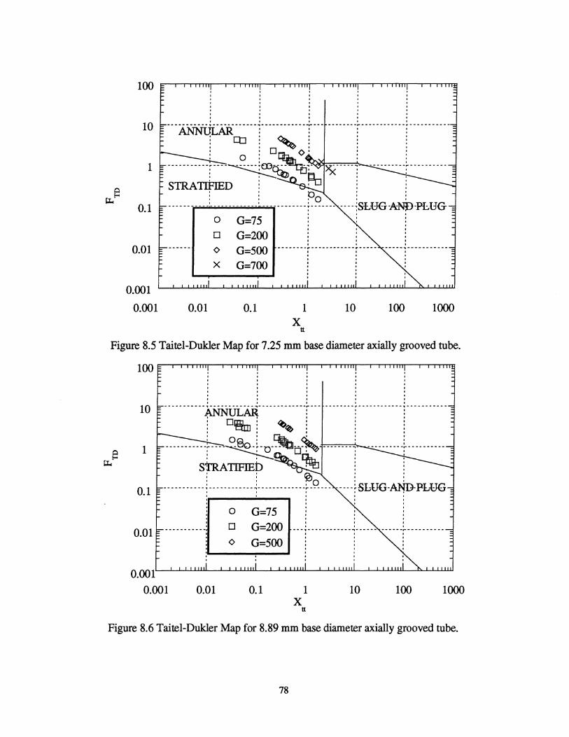
1
Q
r~t .. 0.1
0
0
0.01 <> G=500 x G=700
0.001
0.001 0.01 0.1 1 10 100 1000 X
11
Figure 8.5 Taitel-Dukler Map for 7.25 mm base diameter axially grooved tube.
100
10
1
0.01
0.001
0.001 0.01
o G=75
o G=200
<> G=500
0.1 1 X
11
10 100 1000
Figure 8.6 Taitel-Dukler Map for 8.89 mm base diameter axially grooved tube.
78
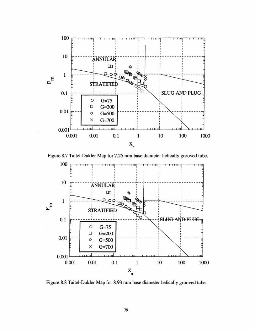
I' I I
-----------~------------~-------------~--- --------r------------.-----------~~ I : :
10 I I I I
: (]] : ~: : : 1 , '" , , -----------~----~£?-~-- --~ --------~ ----------~----------, ~ ~ , ,
SkATIFIEb '-'~ i i , " , " ,
0.1 0 G=75 0 G=200
0.01 G=500
0.001 0.001 0.01 0.1 1 10 100 1000
X n
Figure 8.7 Taitel-Dukler Map for 7.25 mm base diameter helically grooved tube.
100 ~,,~m_,,~~~~~r_,,~=r_.~~_.~on=
" , -----------~~-------------f--- --------r------------1-----------10
• I • I I
: <> : : 1
,
0.1 ----~ SLUG-MiD-PLUG
o G=75 o G=200
0.01
0.001 '--L.......L-.u...u.1.I.I.-~l.....I.....L.Jw.u...__L.....L...L.u..LLI~..L.....L...L_L..U.LLL....__'__~.LJ.LLL___I:I.....L...I...L..U.UJ 0.001 0.01 0.1 1 10 100 1000
X tt
Figure 8.8 Taitel-Dukler Map for 8.93 mm base diameter helically grooved tube.
79

c: o
~ ~ .... o >
100
10 a _______ r ____________ ~-----------
,
<> , 1 --- --- --- --r ----~---qj<><?- -- ---- -- --~---
STRATIFIED ~ , do <><> : : .r-------........ ___ -_____ --+-9--- - --~WG-A~PLU
G=75 : 0.1 a
0 G=150
0.01 <> G=300 x G=450
0.001
0.001 0.01 0.1 1 10 100 1000
1
0.9
0.8
0.7
X tt
Figure 8.9 Taitel-Dulder Map for Graham's data.
--------------p---------------r---------------~------------, , , , , ,
00
: a -_ .. -_ ......... -_ ... --~ ....... --- ""'-e)'" -- --- ..... 0 .............. --:- ......... -- .. _ ..... --- --:- -- -_ .... -- .... _ .. ..
O 6 ----~------- :---------------~---------------i---------------:----- --------. , , , ,
0.5
0.5 0.7 0.8 0.9 Adjusted Premoli
Figure 8.10 Void fraction vs. adjusted Premoli for smooth tubes
80
1

s:: o .... ..... ~ tt "'t:) .... o >
1
0.9
0.8
0.7
0.6
0.5
0.4
0.4
, , , -----------~------------~-------------~------ ---------~-----------, , , , , , , , , , , , , , , , , ___________ ~------------L----------
, , , ,
, , , , ,
, , , , , ------------~------------r------------,-----------, , , , , , , , , , , , , , , , , ,
0.5 0.6 0.7 0.8 0.9 Adjusted Premoli
1
Figure 8.11 Void fraction vs. adjusted Premoli correlation for axially grooved tubes
1
0.95
0.9 I I I I' t --------r---------r---------r---------r---------r---- -- --------~--------I I I I • I I I I I t I I
s:: 0
I I I I I I
I I I I I I I I I I . .= 0.85 ~
tt "'t:) 0.8 .... 0 >
0.75
-------~---------~---------1---------7-------- ------i---------r-------I I I' I I
I I I I I I
, I " I I I I I I I
- - _.- - --~ -- - -- - - - -~-- - - - - -- - -~(j- - 0- - ; -. - . .0- -:-- ------. -~- --- --- - --~- -- --- --: : : :cP: : : : : : n..: : : : _______ ~ _________ ~()---- _______ ~ __ ~ _________ ~ _________ ~ _________ 4 ______ _
1 dO F ~ l ~ ~ 0.7 -- --- --~ ~----;co- ----+ --- -----+ -- ------ -;-- --------;- ---------1- -- --- --
a I : : : : : : o ' 0.65
0.6
0.6 0.65 0.7 0.75 0.8 0.85 0.9 0.95 1 Adjusted Premoli
Figure 8.12 Void fraction vs. adjusted Premoli correlation for helically grooved tubes
81
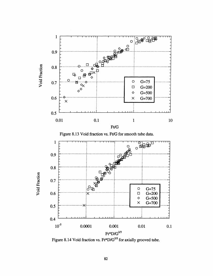
1
0.9
0.8
0.7
0.6
,0 ~O~ , 0 : dfu~ DEl'C:J'!:o' : 0 :
------------------------j----;;-~-~---r------------------------
-----------(}----~----~~~-----------------J------------------------o ¢ 0 :
~ JZ) rfIX: : D tT <> : ,-------,
o ' ---------~ -~ ~------1- ------------------00 i
, <)- - -- - - - - -- - -- - -- - - - - - -~ - - - -- - -- - -- - - - - - - --
x : , ,
o D
o x
G=75 G=200 G=500 G=700
0.5
0.01 0.1 1
FtiG
Figure 8.13 Void fraction vs. FtiG for smooth tube data.
0.9
0.8
0.7
1 : : :dJ r9PD
: ~: 0 o~ , , , , , , -----------------;-------------------;-C;c;- -(j-------;-----------------
, , , , , , , , ,
: ~ : -- ---- ----- --- ----~- --------- --~ , -- -- --- ---- ----- -+------ --- ------ --, ~' , , , , , , , , , ,
------------ --- --~- -----~6 --- --- -~- ------ --- --- ------~ -- ------ ------ ---'~' , , , , , : or.+, : :0 "tJ : 0 G=75
0.6 .. -.... -.. -_ ..... -.. -_ .. -- -:x""" -_ .. -_ .. -_ .......... --:- ... ---- .... _ .. - D G=200 -0 G=500
, , 0.5 .. -- ......... -- ......... -- ~~--- .. -_ .. --- -- .... _ ....... -~- .. -_ .. -- .... - X G=700
, , , , , , , , , ,
10
0.4
10-5 0.0001 0.001
Ft*D/G213
0.01 0.1
Figure 8.14 Void fraction vs. Ft*D/G2I3 for axially grooved tube.
82
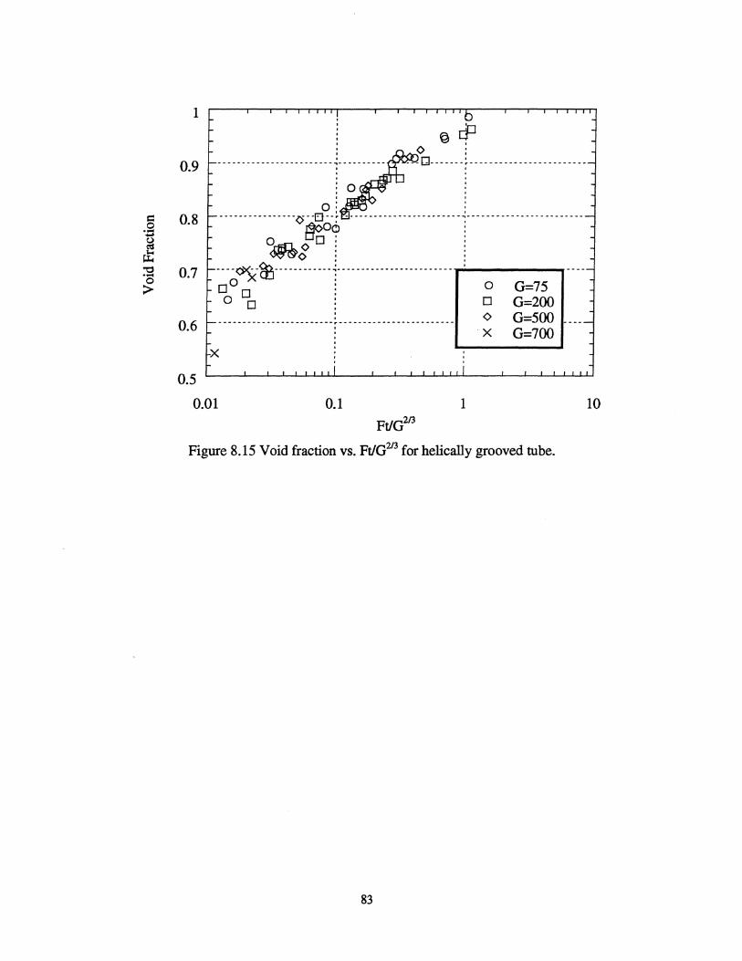
c:: o .... .... ~ tt "'C:j .... o >
1
rF @ . o :
0.9 ------------------------~----------... Q ....... ~ .. _ .................... . , , ,
, . 0.8
O · . .. -_ .. -_ .. -_ .. -_ .. -_ .. X" -0 --~ .... -_ .. -_ .. -- ........ -_ .. -- .......... -!- -_ .. -_ .. -_ .. -- ........ -- ........ --
v~09 :
0.7
orftfi. 0 0 : ~o '
.... ~-~- ...... -.... ~ •••.•..••..•......•.....
Do : o 0 : o : , ,
0.6 ------------------------r-----------------------
x
0.5
0.01
, , ,
.
0.1
FtlG213
.
0 G=75 0 G=200 0 G=500 X G=700
1
Figure 8.15 Void fraction vs. FtlG2/3 for helically grooved tube.
83
.
10

Bibliography
Ahrens, F.W. 1983. "Heat pump modeling, simulation, and design." Heat Pump Fundamentals. Proceedings of the NATO Advanced Study Institute on Heat
Pump Fundamentals, Espinho, Spain, 1980. I. Berghmans, ed. The Hague, Netherlands: Martinus Nijhoff Publishers.
Bankoff, S. G. 1960. "A variable density single-fluid model for two-phase flow with particular reference to steam-water flow." Transactions ASME, Journal of Heat Transfer, Vol. 82, pp. 265-272.
Baroczy, C. I. 1965. "Correlation of liquid fraction in two-phase flow with application to liquid metals." Chemical Engineering Progress Symposium Series, Vol. 61, No. 57, pp. 179-191.
Christoffersen B.C. 1993. "Heat transfer and flow characteristics ofR-22, R-321R-125, and R-134a in smooth and micro-finned tubes." M.S. Thesis, University of illinois.
De Guzman N.M. 1997. "Evaporative heat transfer characteristics in a vertical channel with obstructions." M.S. Thesis, University of TIlinois.
Dobson, M.K. 1994. "Heat transfer and flow regimes during condensation in a horizontal tube." Ph.D. Dissertation, University of TIlinois.
Domanski, P., and D. Didion. 1983. Computer Modeling of the Vapor Compression Cycle with Constant Flow Area Expansion Device. NBS Building Science Series 155.
Graham, D.M. 1998. "Experimental investigation of void fraction during refrigerant condensation." M.S. Thesis, University of TIlinois.
Hughrnark, G. A. 1962. "Holdup in gas-liquid flow." Chemical Engineering Progress, Vol. 58, No.4, pp. 62-65.
Hurlburt, E. T. and T.A. Newell. 1997. "Prediction of the circumferential film thickness distribution in horizontal annular gas-liquid flow." Submitted to Int. I. Multiphase Flow.
Larson, H. C. 1957. "Void fractions of two-phase steam watetmixtures." M.S. Thesis, University of Minnesota.
Levy, S. 1960. "Steam slip- theoretical prediction from momentum model." Transactions ASME, Journal of Heat Transfer, Series C, Vol. 82, pp. 113-124.
84

Lockhart, R. W. and R. C. Martinelli. 1949. "Proposed correlation of data for isothermal two-phase, two-component flow in pipes." Chemical Engineering Progress, Vol. 45, No.1, pp. 39-48.
Maurer, G. 1960. "A method for predicting steady-state boiling vapor fractions in reactor coolant channels." Bettis Technical Review, W APD-BT-19.
Martinelli, R. C., and D. B. Nelson 1948. "Prediction of pressure drop during forcedcirculation boiling of water." Transactions ASME, Vol. 70, pp. 695-702.
NIST 1993. "NIST Thermodynamic properties of refrigerants and refrigerant mixtures", version 4.01. Computer software. National Institute of Standards and Technology.
Panek J.S. 1992. "Evaporation heat transfer and pressure drop in ozone-safe refrigerants and refrigerant oil mixtures." M.S. Thesis, University of Illinois.
Ponchner, M. 1995. "Condensation of HFC-134a in an 18_ helix angle micro-finned tube." M.S. Thesis, University oflllinois.
Premoli, A., D. Francesco, and A. Prina. 1971. "A dimensional correlation for evaluating two-phase mixture density." La Termotecnica, Vol. 25, No.1, pp. 17-26.
Rice, C.K. 1987. "The effect of void fraction correlation and heat flux assumption on refrigerant charge inventory predictions." ASHRAE Transactions, Vol. 93, Part 1, pp.341-367.
Smith, S. L. 1969. "Void fractions in two-phase flow: a correlation based upon an equal velocity head model." Proc. Instn. Mech Engrs., London, Vol. 184, Pt. 1, No. 36, pp. 647-664.
Tandon, T. N., H. K. Varma, and C. P. Gupta. 1985. "A void fraction model for annular two-phase flow." International Journal of Heat and Mass Transfer, Vol. 28, No.1, pp. 191-198.
Thorn, J. R. S. 1964. "Prediction of pressure drop during forced circulation boiling of water." International Journal of Heat and Mass Transfer, Vol. 7, pp. 709-724.
Wallis, G. B. 1969. One-Dimensional Two-Phase Flow. New York: McGraw-Hill, pp. 51-54.
Wattlet, J.P. 1994. "Heat transfer flow regimes of refrigerants in a horizontal-tube evaporator." Ph.D. Dissertation, University of lllinois.
Yashar D.A 1998. "Experimental investigation of void fraction during horizontal flow in smaller diameter refrigerant applications." M.S. Thesis, University of lllinois.
85
Zivi, S. M. 1964. "Estimation of steady-state steam void-fraction by means of the principle of minimum entropy production." Transactions ASME, Journal of Heat Transfer, Series C, Vol. 86, May, pp. 247-252.
86

Appendix A
Smooth Tubes
This appendix presents raw data taken for the 6.12 mm smooth tube. The 4.26
mm smooth tube data appears in Yashar. Data will be presented first in tabular format,
and second in graphical forms.
87

Table A.l Raw data for 6.12 mm inner diameter smooth tube.
88
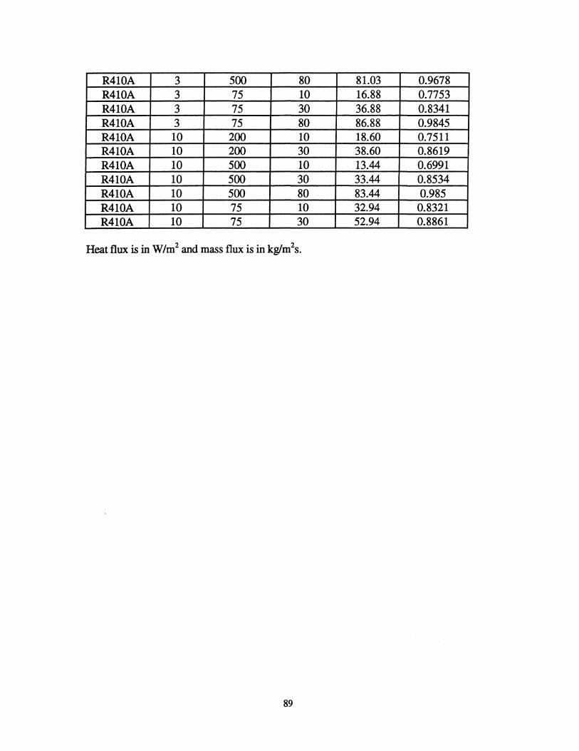
R410A 3 500 80 81.03 0.9678 R410A 3 75 10 16.88 0.7753 R410A 3 75 30 36.88 0.8341 R410A 3 75 80 86.88 0.9845 R410A 10 200 10 18.60 0.7511 R410A 10 200 30 38.60 0.8619 R410A 10 500 10 13.44 0.6991 R410A 10 500 30 33.44 0.8534 R410A 10 500 80 83.44 0.985 R410A 10 75 10 32.94 0.8321 R410A 10 75 30 52.94 0.8861
Heat flux is in W/m2 and mass flux is in kglm2s.
89

s:: o .... ... ~ "t:I .... ~
1
0.8
0.6
0.4
0.2
o
! ! . ! I .: I
: ~: : : I I • I
-- ......... 0. ............ : ... _-_ .......... - .. ----- ... !.. ... _ .. _- -- ....... - -- --: ........ _ .. ----- .. --- --: ..... - .. - ...... -_ ........ --I I • I I I I • I I • I I I • I I • • I
: : : : : : : :
-------------- .. 1 .. --------------~--------- .. -----T------- --------! .... --- ...... -------I : I : · . . · . . : : : · . . I : I I
: I : I ~- ............................ ,. .............................. -:- ............................ -, ............................... -:- ............................. -
: I : • , • • I I : : ....-__ • ___ ....
· . · . · . : I : --------- ...... ---~------ .. --------~---------------:----- .. -. . . · . . · . . · . . I : :
iii
o 20 40 60
Average Quality
o x •
i
80
G=75 G=200 -
G=500
100
Figure A.l Void fraction vs. average quality with a heat flux of 0 W/m2 using R134a in a 6.12 mm inner diameter smooth tube. Mass flux (G) given in kglm2s.
s .... ... ~
d;: "t:I .... o >
1
0.8
0.6
0.4
0.2
o o
. . • 0:
I x: , I I I t O. I I I .. -...... -~-- f ...... -...... --------f------------- .. 1---------------1-- .... ----_ ...... _-I I I I I I I • I I I I
• I I I · .. · .. · .. --- .. -.. -------~------- .. -------~---------------~-------- -------T-------------
• • • I
-------------~---------------T---------------r---------------~-------------I I I I I I I I
: : : ~----.-----.... · . . · · · · . . -------------T---------------~---------------~-----· . . · . . · . . · . . · . . · . . · . . · . .
20 40 60 Average Quality
o G=75 x G=200-• G=500
80 100
Figure A.2 Void fraction vs. average quality with a heat flux of 3 W/m2 using R134a in a 6.12 mm inner diameter smooth tube. Mass flux (G) given in kglm2s.
90

1
0.8
0.6
0.4
0.2
o
! ! ! ! • X I • 0: I
: • X : : 0: I :
I I I I
t--- ..................... ¥ ........................... -:- ............................. ~- ............................... ~ .......................... --o 0 o 0 o 0 o
o o
o 0 0 I I I I
~-------------~---------------~---------------~---------------~---------------I I I I I I , • I I , ,
I I I I I I I I I I • I I I I • o 0 0
---------------~---------------f---------------f---------------~----------------I I , I I I • ,
: : : ,...---0 ___ ...
o G=75 o 0 0
---------------:---------------~---------------r------- x
• G=2oo 1-
G=5oo 0 0 0 o 0 0
o 0 0 o 0 0
o 0 0
o 0 0
i i i I
o 20 40 60 80 100
Average Quality
Figure A.3 Void fraction vs. average quality with a heat flux of 10 W/m2 using R134a in a 6.12 rom inner diameter smooth tube. Mass flux (G) given in kglm2s.
1
0.8
0.6
0.4
0.2
o
! ! l ~ o
o 0 o 0 0
, I I ,
! .: : : ................................. -r"''''' ....... G ............... -:- ............................. -:- ................................ -:- ......................... --
x o
o 0 0
o 0 0 o 0 0 o 0 0
o 0 0 o 0 0
.: : I :
• • I I
---------------~------------- .. -~---------------~---------------:---------------I • I I o 0 0
o 0 0
o 0 0 o 0 0 o 0 0 o 0 0
• • I I
r---"- ............ --- .... ~ .. - .... -- ...... --- .. - .. ~- ---- -- ----- .... -:- --- --- .. -- -- .. - --:--_ .. -- --- --- ---I , I I
I I I I
• , I I : : : ,...--------, o 0 0
o 0 0
o 0 0 o 0 0 ---- .. --- .. -.. -.... -~----- .. -.. -------~---------------!-------0 0
o 0 o 0 o 0 o 0 o 0
i i i
o 20 40 60 Average Quality
o x •
I
80
G=75 G=2oo -
G=5oo
100
Figure A.4 Void fraction vs. average quality with a heat flux of 0 W/m2 using R410A in a 6.12 rom inner diameter smooth tube. Mass flux (G) given in kglm2s.
91

1
0.8
0.6
0.4
0.2
! , , , , ! ! , ,
,
~'U
• , I I : ~ 0: : : ~~-------------~---------------~--------------~------- --------,----------------
x
• o. . I I , , , ,
, , o 0 0
---------------~---------------~---------------~------- --------:---------------I I I I I I I I I t I I I I I I o 0
o 0 , , o ,
---------------~---------------!---------------~---------------~---------------I I I I I I I I : : ~--~o------~ , , , , , , , , ,
~-------------!---------------~---------------~-------, , 0
, , 0 , , , , 0
o 0 , 0
a x
• G=75 G=200 1-
G=500
o ~~~~i~~~~i~~~~i~~~_~I~~~ o 20 40 60 80 100
Average Quality
Figure A.5 Void fraction vs. average quality with a heat flux of 3 W/m2 using R410A in a 6.12 mm inner diameter smooth tube. Mass flux (G) given in kglm2s.
c: o .:;1
~ ~ "0 .~
.0 >
1
0.8
0.6
0.4
0.2
! ! ! !.' I I I I
• 0 o 0 . o· x: 0
I ~: : I -_ ..................................... ~ ................................... -:- .................................... -:- .................................... -:- ............................... --
x: : : : I • I I . : : : : I • • I I I I I
• • I I , I I I
r--------------~---------------~---------------!- ... -- ......................... -.. ~- ...... -.. -.. -- ...... --• I I • • I • I • • I I I I I I O. 0 o. 0 o. 0 o. •
-_ ............................... ~ ....................................... :", ........................... - ....... :... ... _ ............................ !- ...... - _ ..... _ ..... _ .. --I • • I
I • , I
• I I I : : : .------------.1 · . , o 0 0 o 0 0 · , . o 0 0 r-- .. -...... -.. -........ -~ ..... -........ -- ... -- .... -.. ~ .. -... -...... -- ....... -..... ~ .. -... -- .... --o 0
• 0 · . o 0 o 0 · .
o 20 40 60 Average Quality
a x
•
80
G=75 G=200 G=500
100
Figure A.6 Void Fraction vs. average quality with a heat flux of 10 W/m2 using R410A in a 6.12 mm inner diameter smooth tube. Mass flux (G) given in kglm2s.
92

§ .'= ~ tt '0 ..... o >
1
0.8
0.6
0.4
0.2
! ! , ! .: x: · 0 e: I I I I I ,
_ .......... Goo ........ x ~ ............................... :. ............................ -:- ............................. -: ............................ -I I I I , , , o 0 0 o 0 , o 0 0 o 0 0 o , , o 0 0 I • I • I • t I
r--------------~---------------~ .. --------------!---------------!------ ...... ------• I I I , • I • , I I I
• I I I • , I I o 0 0 o 0 0 o 0 0 -_ ......................... -~ .............................. -~ ............................. -~ ................................ -:- ........................... --I I I I I I I • I , I • : : : .--_001...-__ -.
o 0 o 0 o 0
o 0 0
r--------------~---------------~---------------!----- .. -0 0 0
o 0 0 o , 0
o 0 0 o 0 o , ,
o x
•
Q=O
Q=3
Q=lO
--
iii o~~~~~~~~~~~~~~~~
o 20 40 60 80 100
Average Quality
Figure A.7 Void fraction vs. average quality with a mass flux of 75 kglm2s using RI34a in a 6.12 mm inner diameter tube. Heat flux (Q) in W/m2•
§ ..... -~ tt :s o >
1 ! o
! , ! , cpx • • I ox: , • I I I
0.8 r-- ............................................................. :. ............................. -:- ............................... : .................................. -X I I I I
o : : o 0
o 0 o 0 o 0 o 0 0
0.6 I I • I
r--------------~--- ... ------ ... -... --~- ...... ----- ............ -... -~ ... ----- ... --------:---------------· . . . • • I I I I I I I • I I I • I I
• • I I • I I I I • • I
0.4 I I I I ---...... --......... ---... -~ ...... -.. -... ---.. -----:- ............. ---...... -....... -:- ........... ---... ---... ---:- ... -......... --................. -I I I I
• I I I o 0
: ~~------~ o
o 0 o 0.2
o 0 0
~------------ ... ~--- ... ---- ... ------~ ...... --- ..... -.. -- .. -- .. ~---- .. -----o 0 0 o 0 0
x , 0 0
o 0 0 o 0 0 o 0 0 •
Q=O
Q=3
Q=lO o ~~-L~i~~-LJi~~~~i-L~~~CJ~~
o 20 40 60 80 100 Average Quality
Figure A.8 Void fraction vs. average quality with a mass flux of 200 kglm2s using Rl34a in a 6.12 mm inner diameter tube. Heat flux (Q) in W/m2•
93

1 ! o o
o o a<-
! o o o o o
! o o o o o
• I I I
• I I I .... ....a . I , I 0.8 -_ ......... _ ... A - ---~---- ..... ---- .... ---~-- ... ----- .. --- .. --:- .... --- ... -- ..... -- .... -:-- ...... _- ...... - ...... --
0.6
0.4
0.2
0: : : : I I • I I I • I
• I • • I • I I I I I I
• • I I
~------ .. ------~---------------~-------- .. ------!------ .. ------- .. f--- .. -----------I I I I , I • I
I • • I I • I I
o 0 0 o 0 0
o 0 0 o 0 0
I • • I r- .......................... :- .............................. -:- ............................ -:- ............................... '"':- .......................... -I • I ,
I • I I
: : : -----... o 0 0 o 0 o 0 o 0 o 0 0
~-------------~-- .. ------------~---------------~------- --o 0 0 o 0
o 0 o 0 o 0
o 0
o x
-Q=O
Q=3
Q=lO
o ~~~~i~~~~i~~~~i~~~_~I~~~ o 20 40 60 80 100
Average Quality
Figure A.9 Void Fraction vs. average quality with a mass flux of 500 kglm2s using RI34a in a 6.12 mm inner diameter tube. Heat flux (Q) in W/m2•
1 1 I 1 1 ¢ 'A o 0 0
o 0 0
: :. I I
0.8 : • X: : :
~ ............................ -,. ............. G- ............ -,.. ............................. -,- ............................... -,- ......................... --X: : : :
o 0 0
o o 0 0 o 0 0
o 0 0 o 0 0 o 0 0
I I I I
().6 r--------------~------ .. --------~- ... --- ..... -.-.-:------- --------;---------------I I I I I I • I
• • I I
• I I I · . . . · . . . I I • I
• • I I
0.4 r-- --- - -- --- ..... ~ -- ...... - ..... --- .. - - ..... ~- - - ... --- ---- ... - .. -: ......... - ..... _ .... - - .... --:- .. - - - .. - ........... - ---
0.2
: : : _--0 __ - ... o 0 0
o 0 0 o 0 0 o 0 0
o 0 0 o 0 0 ---_ .. _---_._---,_ ..... _----_ .. _----, ..... __ .. _ ...... _----.--_ .... _---o 0 0 o 0 o 0
o 0 o 0 o 0
o 0
o x
-Q=O
Q=3 r-
Q=lO
o~~~~i~~~_~'O~~~~i~~~~i~~~~
o 20 40 60 80 100
Average Quality
Figure A.lO Void fraction vs. average quality with a mass flux of 75 kglm2s using R410A in a 6.12 mm inner diameter tube. Heat flux (Q) in W/m2•
94

s:: o ...... ~ 't:I .-o :>
1
0.8
0.6
0.4
0.2
o
! o o o
! ! o 0
o 0
~x
: x·: : , I 0 I I I
~ ............................. ~ ............................. -~ ............................. -:- ............................. -:- .......................... -0.' , , , X: : : :
I • I •
I , I I I I I I
, " -- .. -_ ... -_ ......... -_ .. ~- .. --- -_ .. ----_ .... ~ ... _-_ .. -_ ....... -_ .. -- ~ -_ .. -_ .. -_ .. -_ ........ ;_ ......... -_ ........ ----I I I I I I I I
I t I •
I I I I I I I I I I I •
I I I I , • I I
f--- .......................... ~ ................................ -~ ............................. -:- ............................. -:- ........................... -I I I I
I I I I : : : r------.., o , 0 , , 0 , , 0
o , , , , , ---------------~---------------~---------------!------- .. , , , , , ,
o , , o , , , , , o 0 0
i i i
o 20 40 60
Average Quality
o x
• I
80
Q=O
Q=3
Q=lO
.-
100
Figure A.ll Void fraction vs. average quality with a mass flux of 200 kglm2s using R410A in a 6.12 mm inner diameter tube. Heat flux (Q) in W/m2•
1
0.8
0.6
0.4
0.2
o
! ! ! , 0 o , 0
o o 0
: 0<.: 0 0 -_ .......................... ~ ............................ -~ ............................. -:- ............................. -;- ........................... -I I , I
I I I I
I I I I . : : : : (¥.: : : :
I I I I t-- .. -- ......... -_ .. -_ .. ~- ... -_ .. -_ .. -_ ... -_ .. -~ ...... - .. -_ ......... -_ .. --: ...... -_ .. -- .... - - -- - ~- - -- - -- - -- - ---I I I 1
" , o 0 , o 0 0
'0 , 0' 0 o 0 0
0' ,
roo ---- --- --- --.. ~ .. --_ .. --- --_ .. -- -~- ---- -- --- --_ .. -:- --- ----_ .... -----:- -- ------ .... -...... -I I I I I I I I : : : .------""'1 o 0 0 , 0 0 , 0 ,
o 0 0 , , , -- ..... -.... - ..... - .. - ... ~ ... --------------~- .. ---- .......... -----!------ .. --o 0 0 o , ,
o 0 0 , , , , , , o 0 0
i i i
o 20 40 60 Average Quality
o x
• I
80
Q=O
Q=3
Q=lO
-
100
Figure A.12 Void fraction vs. average quality with a mass flux of 500 kglm2s using R410A in a 6.12 mm inner diameter tube. Heat flux (Q) in W/m2•
95

1
~ ~~~~::: ~~io~ ..... :,1,~·············· ··o··-,?···· • D=6.12 mm RI34a • D=6.12 mm R410A ..... ' ............. i.Q. . ... . : .o~
, ~ 0 0 i~
0.9 ...
0.8
: ' • 0 : 0.7 ........ ······t·· .... ........ . ............ t· ....•...... ··1··············
0.6
: :.: : • I , ,
0.5~~~~~~~~~~~~~~~~~~~~~~
0.5 0.6 0.7 0.8 0.9 1 Homogenous Correlation
Figure A.13 Void Fraction vs. homogenous correlation showing diameter effects for 4.26 mm and 6.12 mm inner diameter smooth tube.
1
0.9
= 0.8 0 ..... -~ ~ 0.7 "t:) ..... 0
'> 0.6
0.5
0.4
0.4
, , ----- ______ 1 ____________ ~------
, , , , , , .............. -8... .. ........................ ......................... -:-
o : : , , , , , ,
0.5 0.6 0.7
o D=4.26 mm RI34a o D=4.26 mm R410A • D=6.12 mm R134a • D=6.12 mm R410A
0.8 0.9
Rigot Correlation
I
Figure A.14 Void Fraction vs. Rigot correlation showing diameter effects for 4.26 mm and 6.12 mm inner diameter smooth tube.
96

1
0.9
s::: 0.8 0 .... .. ~ 0.7 Lt '0 .... 0
0.6 >
0.5
0.4
0.3 0.3
. ........ -1-· _ .. _ .. ---1-·· -.. _ .. _. f'" --~ .~-. -fl··· ;
: 0:. 0: 0 ~.- : : : : • elI': : : ........ -r . -..... E) .! ... -~ .. -_. r .•....... : .. -........ ! ........... !" ........ . : :.- : : : : I I • I I I .... .. -8 ...... ~ ..................... ~ .. ..... .... .. .. ... .... I ...................... ~ ...................... ~ ................ .... -:- ............... ..
0: : : : ,.----------...,] I I t I
I I • I I I • I .
0.4 0.5 0.6 0.7
Zivi Correlation
o o
D=4.26 R134a
D=4.26 R410A
0.8 0.9 1
Figure A. 15 Void Fraction vs. Zivi correlation showing diameter effects for 4.26 mm and 6.12 mm inner diameter smooth tube.
1
0.9
0.8 s::: 0 .... .. ~ 0.7 Lt ''0 ....
0 0.6 >
0.5
0.4
0.4
···········:·············~···G··· . .
.. I ................. .. -: ........................ -:- .................. -· . · . . • • • : : . : · . . ........ _.£] ......•........•.....•.... : .•.
CiI : : · . · . · .
0.5 0.6 0.7
o o
• • 0.8
· . · . · . · . · . · . D=4.26mm R134a D=4.26mm R410A
D=6.12mm R134a
D=6.12mm R410A
0.9 Ahrens-Thorn Correlation
1
Figure A.16 Void Fraction vs. Ahrens-Thorn correlation showing diameter effects for 4.26 mm and 6.12 mm inner diameter smooth tube.
97

§ • .::;1
~ d:: '0 .... o >
1
0.9
0.8
0.7
0.6
0.5
. . . -~·-----------r---------------~---------------~------- ----~~ , , , · . · · ·
·
:0
---------y-------------,
: ~ 0 ri:J : : : .: 0 : :
------ --------~ -- --1-------- . ----- -------- --~ ------- --------:---------- ----· . · · · · , · , · --------------~---------
0.6
· · · , · · , · 0.7
o o • •
0.8
Smith Correlation
D=4.26 mm RI34a D=4.26 mm R410A D=6.12 mm R134a D=6.12 mm R410A
0.9 1
Figure A17 Void Fraction vs. Smith correlation showing diameter effects for 4.26 mm and 6.12 mm inner diameter smooth tube.
r:: o • .::;1
1
0.9
~ 0.8 Ii: '0 .... ~
0.7
0.6
0.5
. · : 0
-------------J---------------~-------tl-()-: : 0 : . · · · ·
o
--------------r---------()---
0.5
· · · · · · · : -1:}----------~------------· 0
0.6 0.7 0.8
· , ------T-------------· · · · , · , · ·
o D=4.26 mm RI34a o D=4.26 mm R410A • D=6.12 mm R134a • D=6.12 mm R410A
0.9 1
Domanski Correlation
Figure A.18 Void Fraction vs. Wallis correlation showing diameter effects for 4.26 mm and 6.12 mm inner diameter smooth tube.
98

c: 0
'.:1 ~ ~ "t:I .-0 >
1
0.9
0.8
0.7
0.6
0.5
----------~------------~-------------~------------ ------~~ , , , , , , , , , , , , , , I I I I
......... ··t········· ... t·~· ~ .. 1!.J... ! ........... ·t··· ....... . : o:.Ll 1~ : :
-----[j----r---------~~---ilt----- i------------i-------------r----------
-----G- ---:- ----------- : ------------: p , , , ,
o D=4.26mm R134a
o D=4.26mm R1410A • D=6.12mm R134a
D=6.12mm R410A
0.4 ~~~~~~~~~~~~~~~~~~~~~~
0.4 0.5 0.6 0.7 0.8 0.9 1
Baroczy Correlation
Figure A.19 Void Fraction vs. Baroczy correlation showing diameter effects for 4.26 mm and 6.12 mm inner diameter smooth tube.
c: o .--~ ~ "t:I .-o . >
O.
O.
o 0: , ,
O. -----------O-~---fi---.----: -------.----,..r-----------.......
O.
, ,
~ .. o D=4.26 mm RI34a o D=4.26 mm R410A • D=6.12mmRI34a • D=6.12 mm R410A
O.~~~~~~~~~~~~~~~~~~~~~~~
0.5 0.6 0.7 0.8 0.9 1 Tandon Correlation
Figure A.20 Void Fraction vs. Tandon correlation showing diameter effects for 4.26 mm and 6.12 mm inner diameter smooth tube.
99

5 .... i "0 .... ~
• , , I
: : : --O. -------------+--------------+ ---------------)--------.- ~ -------------
O.
: : 0: if : : : 0 I
-------------j------------��-~-----iS?JIlII-· -------------~-------------: : 0 : :
:0 . · · · ·
o. --------------~--g--Cb------i -------o o
· · · D=4.26 mm RI34a D=4.26 mm R410A
O. · · · --------------,--------· · · · ·
• D=6.12 mm R134a II D=6.12mmR41OA
O.~~~~~-L~~~~~-L~~~~~~~~~~
0.5 0.6 0.7 0.8 0.9 1 Premoli Correlation
Figure A21 Void Fraction vs. Premoli correlation showing diameter effects for 4.26 mm and 6.12 mm inner diameter smooth tube.
5 '':= ~
d:: "0 .... o >
1
0.9
0.8
0.7
0.6
0.5
0.5
II 110 IIll
II II --------------f-(j--~----
· · · · · ·
0.6 0.7
o D=4.26 mm RI34a o D=4.26 mm R410A • D=6.12 mm RI34a -II D=6.l2 mm R410A
0.8 0.9 Hughmark Correlation
1
Figure A.22 Void Fraction vs. Hughmark correlation showing diameter effects for 4.26 mm and 6.12 mm inner diameter smooth tube.
100

§ .:;1
~ ~ "tj .... o >
1
0.9
0.8
0.7
0.6
0.5
0.5
o D=4.26mm RI34a
o D=4.26mm R410A
• •
D=6.12mm RI34a
D=6.12mm R410A , , , , o
-----~-------------, , , , ,
-------------~---------------~---[j----------, ••
1 0..· 10 • • I '.. : • Dc;, rI' :. :
........................................ ~ ........... -- ...................... ' ..................................... -iIC=>- ............................. -:- ................................. ... : Q:. :
o : : • : : 0 , : · :.: : -------------. --------------~----------1II--!---------------;--------- ----: : ~ : • • I I • • I I
• I I I , I I I
0.6 0.7 0.8 0.9 Graham Correlation
1
Figure A23 Void Fraction vs. Graham's condenser correlation showing diameter effects for 4.26 mm and 6.12 mm inner diameter smooth tube.
101
AppendixB
Axially Grooved Tube
This appendix presents raw data taken for the 8.89 mm base diameter axially
grooved tube. The 7.25 mm base diameter axially grooved tube data appears in Yashar.
Data will be presented first in tabular fonnat, and second in graphical forms.
102

Table B.l Raw data for 8.89 mm base diameter axially grooved tube
~~~~~~ R134a 0 200 10 10.00 0.7042 R134a 0 200 30 30.00 0.8706 R134a 0 200 80 80.00 0.9623 R134a 0 500 10 10.00 0.7501 R134a 0 500 30 30.00 0.9006 R134a 0 75 10 10.00 0.7070 R134a 0 75 30 30.00 0.8242 R134a 0 75 80 80.00 0.9541 R134a 3 200 10 12.15 0.7508 R134a 3 200 30 32.15 0.8803 R134a 3 200 80 82.15 0.9680 R134a 3 500 10 10.86 0.7774 R134a 3 500 30 30.86 0.9173 R134a 3 75 10 15.72 0.8025 R134a 3 75 30 35.72 0.8723 R134a 3 75 80 85.72 0.9805 R134a 10 200 10 17.15 0.8099 R134a 10 200 30 37.15 0.8862 R134a 10 200 80 87.15 0.9867 R134a 10 500 10 12.86 0.8206 R134a 10 500 30 32.86 0.9229 R134a 10 75 10 29.07 0.8768 R134a 10 75 30 49.07 0.9160 R410A 0 200 10 10.00 0.6236 R410A 0 200 30 30.00 0.7963 R410A 0 200 80 80.00 0.9574 R410A 0 500 10 10.00 0.6723 R410A 0 500 30 30.00 0.8371 R410A 0 75 10 10.00 0.6448 R410A 0 75 30 30.00 0.7885 R410A 0 75 80 80.00 0.9432 R410A 3 200 10 11.79 0.6528 R410A 3 200 30 31.79 0.8246 R410A 3 200 80 81.79 0.9636 R410A 3 500 10 10.72 0.6808 R410A 3 500 30 30.72 0.8474 R410A 3 75 10 14.78 0.7000 R410A 3 75 30 34.78 0.8264
103

R410A 3 75 80 84.78 0.9870 R410A 10 200 10 15.94 0.7409 R410A 10 200 30 35.94 0.8488 R410A 10 200 80 85.94 0.9730 R410A 10 500 10 12.39 0.7002 R410A 10 500 30 32.39 0.8505 R410A 10 75 10 25.94 0.7873 R410A 10 75 30 45.94 0.8909
Heat flux in W/m2 and mass flux in kglm2s.
104

§ • .:= ~ ~ ~ .... o >
1
0.8
0.6
0.4
0.2
o o
o --------------~---------------~---------------~---------------~-------------
<> C
I I I ,
• I • I • t , I
• I I • · .. · .. · .. · .. · .. · .. -------------,---------------,---------------T---------------y-------------
• I I I ................................ .- ............................ -I'" ................................... ,- .................................... -,- ............................... -I I • I · . , . : : : ~--~----~ · . · . · . · . · . .
-------------,---------------,---------------9-----
20 40 60 Average Quality
o o
G=75 G=2oo -
<> G=5oo
80 100
Figure B.l Void fraction vs. average quality with a heat flux of 0 W/m2 using R134a in a 8.89 mm base diameter axially grooved tube. Mass flux (G) given in kglm2s.
c o . .:= ~ ft ~ .... o >
1 ! ! ! !X O I I I I . : ' : Xo : . : I • I I
0.8 1--- .................... -0 ...... ~ ................................... -:- ................................. ..:- ................................ ~ ................................. ---X: : : :
• I • • , I I I .. . .. . .. . • , I I
0.6 • I I I ~ --- -- -_ .. --_ ..... -:'"' ....... -- _ ... -- --- .... ~ .. -- ..... '"' .. -_ .... --_ .. ~ .. -_ .. -_ .. -_ .. --.. --~- --- _ .. -_ .. -_ ... --I I I I I • I •
• • • I I I I I
• I I • • I I I I I I I I , I I
0.4 ---- .. -- .. ---- .. --~- ... ----- .... -- .. -.. -!- .. -... -.. -.. -------~-- .. ---- .. --- ......... ~----- ..... --------I I t I
: : : ~---' ------... · . . · . · . o G=75 · . ().~ ~-------------:---------------r---------------r------ x G=2oo f-· . · . · . · . • G=5oo · .
o i i i I
o 20 40 60 80 100
Average Quality
Figure B.2 Void fraction vs. average quality with a heat flux of 3 W/m2 using R134a in a 8.89 mm base diameter axially grooved tube. Mass flux (G) given in kglm2s.
105

c:: o ...... ~ ~ "0 .-o >
1 ! ! ! ! u ,
0 , , ,
0 , , , ,
0 0 , , , I I I •
0.8 <> I I I I
i.....-_ .................... '0 .. ~ ............................ _~ ............................ _~ ............................ _;_ .......................... _ I I I I
I I I I
I I I I I I I I
I I , I
I I I I
" , I I I I
0.6 1-- .......................... ~ ............................... ~ .............................. ~ .............................. ~ .......................... -I I I I • I I I
I I t I
J I I I , I • I
I I I I I I I I I I I I
0.4 --- .......... - ... -.. ---~ -_ .... -- -- .. -- .... --~ .... -- .. -_ .. -_ .. -_ .. -~ .. -_ .. -_ .. -_ .. -_ .. --:- -- ...... -...... -.... --I I I •
: : : ----' ----. , , , , , , , , , , , , , , , 0.2 I---------------~---------------~---------------~--------, , , , , , , , , , , , , , , , , ,
o o
G=75
G=2oo
G=5oo
o ~~~~i~~~~i~~~~i~~~~I~~~~ o 20 40 60 80 100
Average Quality
Figure B.3 Void fraction vs. average qUality with a heat flux of 10 W/m2 using R134a in 8.89 mm base diameter axially grooved tube. Mass flux (G) given in kglm2s.
c:: o .= ~
."0 .-o >
1 ! ! !
* , , , , , , , , : _: : :
0.8 r.--"" -- .. --- -_ .. --~ ...... _ .... ~--- .. -- -~- .. -_ .. -_ .... - .. -_ .. -:- .. -- .................... --;- .. _ .............. -- .. --
0.6
0.4
0.2
o
, , , I I I I I I I I
I I , • ~
' , , ,
------- ................ ~ .... ----------- .. -~----- .... --------~---------------~--- .. -- .... -------I I I I I I I I
I I I I I I I I I , I •
I I I I I I I I I I I I
rOo ...... ---.... --...... ~ .......... ---.. -.... -.. -~ -......... --........... - .. -:- --.... -................. --:- ................. -...... --I I I I : : : r----------, , , , , , , , , , , , , , , , , , ,
-- .... --- .. -- .. -- .. ~---- .... - ... -- ....... --~ .. ---- .. ------- .... ! ........ - .. , , , , , , , , , , , ,
i i i
o 20 40 60
Average Quality
o x
• i
80
G=75 G=2oo .
G=500
100
Figure BA Void fraction vs. average quality with a heat flux of 0 W/m2 using R410A in a 8.89 mm base diameter axially grooved tube. Mass flux (G) given in kglm2s.
106

1 ~~~~~~~~~~~~~~~~~~~~~~ l l l lx l!) · . · . · . • , • I
0.8 • •• I • I : -xo: : : f--- .......................... ~ ........................... .. -:- .............................. -:- ............................. -:- ......................... "'-
· . · . ~o ! ! . .
0.6 I I • I -- .. -.. -- .. -.. ---- .. ~ .. ------------- .. ~-- ...... -.. --------! .. ------ -----_ .. _;---------------• I I • • , I • • , I I I I • I · .. · .. , " .. .
0.4 ~ ............ -... --- .. -.. ~ ........ _ .......... __ ..... _-:--- -.. ---- .. -.......... -:- ... _ .... -................ --:---- ............... -.. --
0.2
· , . . I I I •
• I I I
: : : ...------.......... · . · . , , · . . --- .. -----------~------------ .. --~---- .. ----- .. --- .. !----- .. -. . . · . . , , . · . . · . . , . ,
o 20 40 60 Average Quality
a x e
80
G=75
0=200
G=500
-
100
Figure B.5 Void fraction vs. average quality with a heat flux of 3 W/m2 using R410A in a 8.89 mm base diameter axially grooved tube. Mass flux (G) given in kglm2s.
1
0.8
0.6
0.4
0.2
o
! ! ! ! x , · , , , · · · : a · · , , ex · · : · · , ,
, I • I -_ ........................... ~ ...... 0 ............... ..... -:- ................................ -:- .............................. -: ............................. -• • • I
X : : : : e : : · , · . I • I I
I I I I
~- .. -.. ------ .. -.. ~ .. --- .... -- .. ---- .... ~- .. ------------ .. ~------- --------;---------------I I I I , I • I
I t I I
• I I I • • I I • • I I
• I I I • I I I
~ ... _ ......... -.......... -_ .. ~ _ .... --_ .... _ ...... _ .. -~ ........ _ ......... -................ ~ ............ --.. _ ................. ; .................... - ............ -I I • I
• I , I · . . . : : : ~----......., · . . · . . · , , · . . -- .............. -............ -~ ...... -................................. ~- ....... --- ..... --- .. --~ ...... ----· . . · . . , . . · . . · . . , , ,
iii
o 20 40 60 Average Quality
a
x e
80
G=75
G=200
G=500
-
100
Figure B.6 Void fraction vs. average quality with a heat flux of 10 W/m2 using R410A in a 8.89 mm base diameter axially grooved tube. Mass flux (G) given in kglm2s.
107

1
0.8
0.6
0.4
0.2
o
! ! ! , , , 6 x : :.: : • X: : I
: 0: : : ~----------x --~ ---------------~ ---------------~ ---------------,- --------------
o • I I I
" , , , , ,
. . ,
, , , . --- .. ----------~---------------~---------------~------- --------:---------------
I I • I
, " , .. , " , , , ,
t-- ........................... -~ ................................. -~ .................................. -:- .................................... -:- ................................... -, • I •
I : : ~~' ______ ~
, , , , , , , ,
---------------~---------------~---------------!------- ...
i i i
o 20 40 60 Average Quality
o x
• i
80
Q=O Q=3 Q=lO
-
100
Figure B.7 Void fraction vs. average quality with a mass flux of 75 kglm2s using R134a in a 8.89 mm base diameter axially grooved tube. Heat flux (Q) in W/m2_
c: o .= ~ ~ -0 .... ·0 >
1
0.8
0.6
0.4
0.2
e: , 0>< , I I I I
................................ ~ .............................. ........ !,. .................................... :.. ................................... -:- ........................... .. • • I I
X: : : : 0: : : : • I I • • I • I • I • I I I • I
, .. ..................................... r ............................ ... -r ...................................... -I" ................................... -,- ............................... ..
. ------- .. -----~---------------~---------------y--------
o X
Q=O
Q=3
• Q=10
o ~~~~~~~~~~~~~~~~~~~~~~ o 20 40 60 80 100
Average Quality
Figure B.8 Void fraction vs. average quality with a mass flux of 200 kglm2s using R134a a 8.89 mm base diameter axially grooved tube. Heat flux (Q) in W/m2•
108

1
0.8
0.6
0.4
0.2
! ! 1 1 ,
~ , , , , , , ,
, ,
I I I I
• I I I I
1--- ............................... ~ ................. ............ -:- ............................ -:- ............................. -:- ....... ...................... -
CS: : : : I I I I I , I I
I I I •
I I I I I I I I
I I I I
r--------------~---------------~---------------;------- --------:---------------I I I I I I I I
I I I I
I I I I • I I I
I I I I
• I I I , , , 1--- ............................. ~ ............................ -:- .............................. -: ................................ -:- ............................ -
I I I ,
: ~--~-----, , , , ,
r--------------~---------------~---------------~------- ... , , , , , , , , , , , , , , , , , ,
o 20 40 60 Average Quality
o x
•
80
Q=O
Q=3 -
Q=lO
100
Figure B.9 Void fraction vs. average quality with a mass flux of 500 kglm2s using R134a in a 8.89 mm base diameter axially grooved tube. Heat flux (Q) in W/m2•
s:: o .... ....
~ ~ .... o >
! ! ! , , 1 I X.
Ci' I • I I
, I I I
: x: : : 0.8 1--- --- - -- - -- - - -: -- -.-0- ----- -:- --- --- --- --- --:- ------ ------ ---:- -- --- --- ------, ,
X : : : , , , 0: : : I
0.6 r"''''-''''''''' - ..... -_ .. ~- ... -- .... -- -_ .. -_ .. -~ .. -_ .. -_ .. -- .. -_ .. --: .... -- .... -_ ... -- ........ ;- ........ -- ........ ---I I I I I I I •
I I I I I I I I
" , " , " , " ,
0.4 1--- - - - - -- - -- - - -~ -- - -- - - - - -- --- -~- - - - - -- - -- - - - - -!- --- --- --- --- ---!- -------- --- ---I I I I
: : : ~~'-------, , , , , , , , , 0.2 t- - - - - - - - - - - - - - ~ - - - - - - - - - - - - - - - ~ - - - - - - - - - - - - - - - i ---------
, , , , , , , , , , , , , ,
o x
•
Q=O
Q=3
Q=lO iii o~~~~~~~~~~~~~~~
o 20 40 60 80 100
Average Quality
Figure B.1O Void fraction vs. average quality with a mass flux of75 kglm2s using R410A in a 8.89 mm base diameter axially grooved tube. Heat flux (Q) in W/m2•
109

1
0.8
0.6
0.4
0.2
o
• • I I
: . : : : ............................ ~ ............ &- .... ....... :., ............................... :- ............................... : ............................. -I I I I . : : : :
o 0 0
o 0 0 o 0 0 _x 0 0
-----~~-----,------ .. --------~ .. --------------~------ .. -.. ------1-------------I I I I
• I I I I I • I , I I I
, I I I I • I I I • I I
If' I o 0 0
I I • I ............................... po .......................... ........ ,.. ............................................................... -.- ............................ ...
o 0 0
o 0 0
o 0 0
-------------,------------ .. _ .. ,---------------.-------o 0 0 o 0 0 o 0 0
o 0 0 o o o o
20 40 60
Average Quality
o x
•
o
80
Q=O
Q=3
Q=lO
100
Figure B.ll Void fraction vs. average quality with a mass flux of 200 kglm2s using R410A in a 8.89 mm base diameter axially grooved tube. Heat flux (Q) in W/m2•
1
0.8
0.6
0.4
0.2
o
! ! ! ! 0 0 0 0
0 0 0 0
0 0 0
C!I' 0
0 : 0 0 , I • I
~- ............................. ~ ............................. -:- ............................ ""!- ............................... ~ ............................... -• I • I I t I I
I I I I
ttl' ~ ~ : ~ • • I I I I I I -------- .. ------~---------------~--- .. -----------~------- --------:---------------I I I I , , I f
f , I •
• I I • I , , ,
I , • •
I I I I o 0 0
~------.------~---------------!---------------:.--.-----------~---------------I • I • I • • I
: : : ~ __ o ______ ~
o 0 0 o 0 0 o 0 0
---------------!---------------~---------------~------- --o 0 0 o 0 0 o 0 0
o 0 0 o 0 o 0 o 0
i i i
o 20 40 60
Average Quality
o x
• 80
Q=O Q=3
Q=1O
100
Figure B.12 Void fraction vs. average quality with a mass flux of 500 kglm2s using R410A in a 8.89 mm base diameter axially grooved tube. Heat flux (Q) in W/m2•
110

1
0.95
0.9
c:: 0.85 0 .,:j
~ tt 0.8 "0 .... 0 > 0.75
0.7
0.65
0.6
0.6
o o <>
• • •
R134aG=75 R134aG=200 R134aG=500 R410AG=75 R41OAG=200
, • • I I I I
I I I I I I •
... ----~---------~---------.---------~---------!---.----~~iE1------~-------I I I I • I I I I I I • I , • , • I • I I
I I I , I I I
...................... ~ .......................... ' ..................... ~ ....................... :.. ........... -..... : ......... Q .. :- ................... :- ............. .. I I I I • I I • , • •• I I I
: : : .: : : :
0.65 0.7 0.75 0.8 0.85 0.9 0.95
Homogenous Correlation
1
Figure B.13 Void fraction vs. homogenous correlation for 8.89 mm base diameter axially grooved tube using R134a and R41OA. Mass flux (G) in kglm2s.
1
0.9 o D=7.25 mm Rl34a
o D=7.25 mm R410A
c:: 0.8 0 .,:j
~ tt 0.7 "0 .... 0 '>
D=8.89 mm Rl34a
• D=8.89 mm R410A ~ 0 0
: : : : rP im -----------:-------------;----------- . -------0-,.-'---r1'-- :-----------: : : .: I I I I I • I I I I I I
•
0.6 ----------~----------- I ------- ... --rj-------------~------------~----------I I I I
. . . 0.5 .......................... ~ ........ G ........... ~ ............................ ~ ........................ -:- .................. ..
I I • I • , I ,
• I I ,
I I • I I , I I
0.4
0.4 0.5 0.6 0.7 0.8 0.9 1
Homogenous Correlation
Figure B.14 Void fraction vs. homogenous correlation for 7.25 mm and 8.89 mm base diameter axially grooved tubes using R134a and R41OA.
111
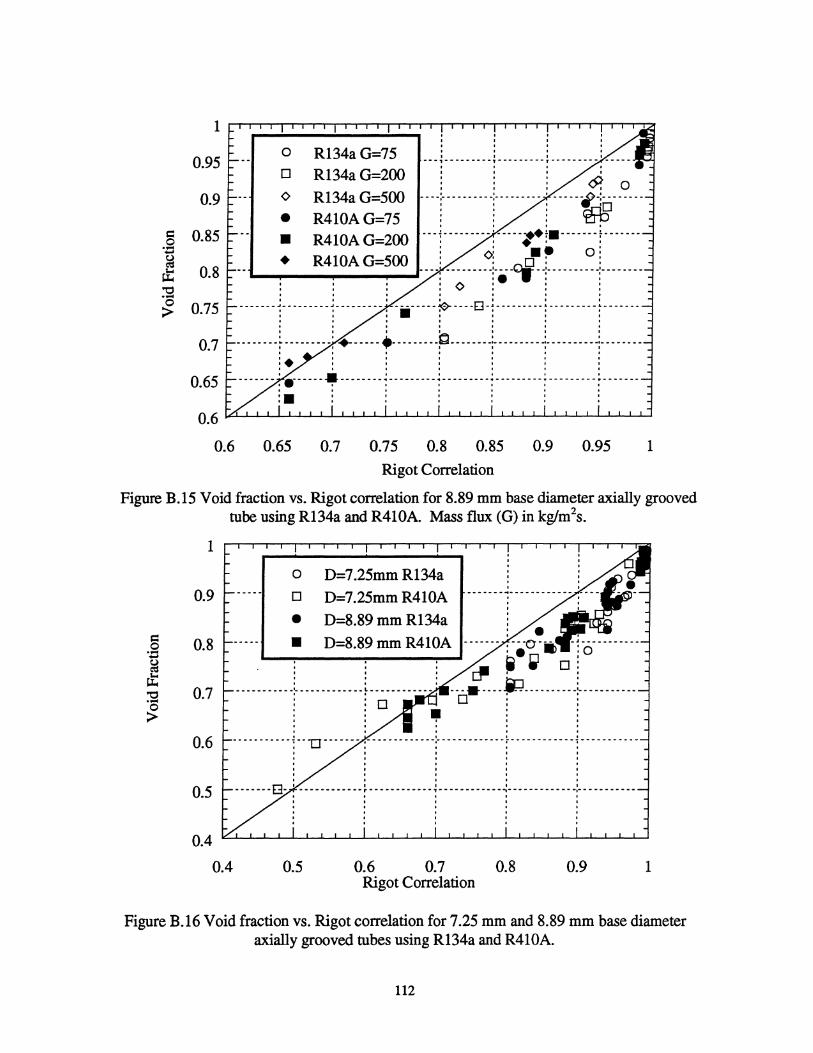
c:: o .~
g ~ "0
--or --------r -------i -----~ ---------i---------:-----~~tll-------t-------
I •• I I : ' .~ 0: ........ I ................ _:_ .... _~ ...... :_ ................... _:_ ............ ..
: 0 :-.: : I I I •
I I I I • I I
.... -----~---------~---------f -.------ .. ~ .. ---E3-!---------~---------~-------I I I • I I I
~ 0.75 • I I • I • I • I • I , I •
O 7 ----- ---~ -------- .. : ~- .. -_ .. ~--- ---- .... FJ---- ----~----- .. -_ .. -~- .. -.... ----~- --- -...... . """ I I I I I I I I I I I I I I I I I I
0.65
O. 6 1oLL-J....J....L...l......L-.J.....L...L....L....J....J.....L....L-J....J....L...l......L....L...L...L....L....J....J.....L.-L-~"'_'_ .............. ...L...L....L....J....J.....L....I
0.6 0.65 0.7 0.75 0.8 0.85 0.9 0.95 I
Rigot Correlation
Figure B.15 Void fraction vs. Rigot correlation for 8.89 mm base diameter axially grooved tube using R134a and R410A. Mass flux (G) in kglm2s.
I
0.9
c:: 0.8 0 .~
g ~ "0 .... 0.7 0 >
0.6
0.5
0.4
D=7.25mm R134a
D=7.25mm R410A
• D=8.89 mm Rl34a
• D=8.89 mm R410A
, , __________ .. ~ ___ ---------L------------, , I ,. I , , , ------------r------------,------------,-----------, , , , , , , , , , , , ,
0.5 0.6 0.7 0.8 0.9 Rigot Correlation
I
Figure B.16 Void fraction vs. Rigot correlation for 7.25 mm and 8.89 mm base diameter axially grooved tubes using R134a and R41OA.
112

1
0.9
0.8
<II :0
----- --- -----.---- -e Q- ---.. : e .:
0 R134aG=75 0 R134aG=200
<> R134aG=500
0.7
• e R41OAG=75 0.6 • R41OAG=200
• R41OAG=500 0.5 1L...1--.J..........L..-L-..L-.I-...1--.J..........L..-L--l..-.I-...1--.J...--W ..... ______ ~
0.5 0.6 0.7 0.8 0.9 1
Zivi Correlation
Figure B.17 Void fraction vs. Zivi correlation for 8.89 mm base diameter axially grooved tube using R134a and R410A. Mass flux (G) in kglm2s.
1
0.9
0.8
= 0 0.7 .::: ~ ~ 't:I .... 0.6 0 >
0.5
0.4
0.3
0.3
: : : :. ................... ~ .................... ~ ..................... -!- ................... -p ...... :;.:~~ •• ~
: : : e, : 1 1 1 ~ 1e 10 1
..... --_ .. _ .. ~- ............ -----: ........ --- ............. -~-.. ..- ----:- .. -- --_ ....... -t ..... _____ .. 00
o ;_0: 0: : : : .: : : :
• I I I I I
I I I I I ........ --- ..... :0- ........ ----:- ............. --- I ............................................. " ........................ I ................... _ .
o D=7.25mm R134a --E3---~----------' ---------~--- o D=7.25mm R410A
e D=8.89mm R134a
· . . • • I · . . · . I I · .
0.4 0.5 0.6 0.7 0.8 0.9
Zivi Correlation
1
Figure B.l8 Void fraction vs. Zivi correlation for 7.25 mm and 8.89 mm base diameter axially grooved tubes using R134a and R41OA.
113

= 0 '.::l ~ It "0 .~
0 >
1
0.95
0.9
0.85
0.8
0.75
0.7
0.65
o o <>
• •
R134aG=75 R134aG=200 RI34aG=500 R41OAG=75
R4I0AG=200
.' ~: 0
.' t;.7" • .............. :- _ ... _ .......... -! .. - ................. .. ...... --(>.; --'- -_ .. -_ .. ...
: : : ':~rb I • I ~
-.... -~- ..... -... ----: ... ------~II--- .. --~- .. -... ---I •• •
• R41OAG=500 : <> ~ 0 ... 0: : : : ---- ; ---------1-°.--1-1----------1--------: : : ~ : : : : : : I : : : ......... - ... -~- ........ - ........... ~-- ... -- ... - ... - - ... ---~-1 ... --E3----T-- ...... --- .... y-- .. - .. ----~---- ...... -
: : : -: : : : I I I • t ' • I • : t I I
: : : A· : : : .......... _ ...... i....... ............ .. ........... --too -e- -~-~ ..... -......... --........ _ ............ _,_ ..... -............. 1 ............... ...
: I : • • : :
· ·
0.6 0.65 0.7 0.75 0.8 0.85 0.9 0.95 Ahrens-Thorn Correlation
1
Figure B.19 Void fraction vs. Ahrens-Thorn correlation for 8-89 mm base diameter axially grooved tube using R134a and R410A Mass flux (G) in kglm2s.
1
0.9
= 0.8 0 .~ .... ~ It "0 .~
0.7 0 >
0.6 _ ... _-_ .. ------}------ 0 D=7.25mm RI34a · · · 0 D=7.25mm R410A · 0.5 • D=8.89 mm RI34a
• D=8.89 mm R4I0A
0.4
0.4 0.5 0.6 0.7 0.8 0.9 1
Ahrens-Thorn Correlation
Figure B.20 Void fraction vs. Ahrens-Thorn correlation for 7.25 mm and 8.89 mm base diameter axially grooved tubes using R134a and R4I0A.
114

1
0.9
0.8
0.7
0.6
0.5
: : : <:f> ......................................... ~ .................... ................. : ......................................... .: ........................ ~ ........... ... ................................ ..
I I • I .. . .. . .. . .. . · . · .
. · . --- --- --- ---- ~----+-. ---Q' - --- -- --- --- ---.. : · . : ill :
0.6 0.7 0.8
Baroczy Correlation
0
0
<>
• • •
. .
R134aG=75 R134aG=200 R134aG=500 R41OAG=75 R41OAG=200
R41OAG=500
0.9 1
Figure B.21 Void fraction vs. Baroczy correlation for 8.89 mm base diameter axially grooved tube using R134a and R41OA. Mass flux (G) in kglm2s.
1
0.9
= 0.8 0 .p ~ It 0.7 "0 .-~
0.6
0.5
0.4
0.4 0.5 0.6 0.7
o o D=7.25mm R410A
• D=8.89 mm Rl34a
D=8.89 mm R410A
0.8 0.9
Baroczy Correlation
1
Figure B.22 Void fraction vs. Baroczy correlation for 7.25 mm and 8.89 mm base diameter axially grooved tubes using R134a and R41OA.
115

c:: o ..... .....
~ "0 ..... o >
I
0.9
0.8
0.7
0.6
0.5
0.5
• .9.' 0 car:@ I I I. : : : 0 <5>
--------------~---------------~---------------~-----~------ -----------.-, , .' nO : : 0 bc:t
: : .' , , : :~,
-------------~---------------1----(J----1*-:;:---------------?-------------: : •• .A: : f I V I I
0 R134aG=75 0 R134aG=200
..
0 R134aG=500
• R41OAG=75
• R41OAG=200
• R41OAG=500
0.6 0.7 0.8 0.9 Hugbmark Correlation
I
Figure B.23 Void fraction vs. Hugbmark correlation for 8.89 mm base diameter axially grooved tube using R134a and R41OA. Mass flux (G) in kglm2s.
c:: o ..... .....
~ "0 ..... o >
I
0.9
I • I • I
0.8 -----------:------------:-------------~--~~ts·~:------------:-----------I I I f I I I I
• I I I
• I I I •• I I , , , ,
----------~-------------~----------, , -----------~------------~------0.7 , , , , , ,
0.6 ···········~······D···· : ........... . o 0=7.25mm R134a
0.5
0.4 0.5
o 0=7.25mm R410A
• 0=8.89 mm RI34a
0=8.89 mm R410A
0.6 0.7 0.8 0.9 Hugbmark Correlation
I
Figure B.24 Void fraction vs. Hughroark correlation for 7.25 mm and 8.89 mm base diameter axially grooved tubes using RI34a and R41OA.
116

1
0.9
c: 0.8 0 ..... ..... ~ d: 0.7 '0 ..... 0 >
0.6
0.5
0.4
0.4
o G=75 R134a
o G=200 R134a
<> G=500 R134a
• G=75R41OA
• •
G=200R41OA
G=500R41OA ~ : I
-----:~---:----•• -:----~rr---.~--·--------~-----------tJ .: 0
o --- ------- -;- --- --- --- -- : -.- ~- --- -! ---- --- --- --~ --- --- --- ----;-- --- --- ---
I I I I I
: : ~ : : I I I.
o 0 0
0.5 0.6 0.7 0.8 0.9
Graham Correlation
1
Figure B.25 Void fraction vs. Graham's condenser correlation for 8.89 mm base diameter axially grooved tube using R134a and R41OA. Mass flux (G) in kglm2s.
1
0.9
I I I I
s .~
~ '0
0.8
0.7
-----------~------------~-------------~------ -- ---------~-----------o 0 0 __ ~,_
o 0 0
o 0 0 o 0 o 0 o 0 0 o 0 o 0
-----------~------------~----------o 0
o 0 ..... o >
0.6
o
o 0 0 ......... -.... -.. -- ~ .. -.. -_ .. -n-" :- --_ ........ --_ .. --:- ...... 0 D=7.25mm RI34a o 0 0 o 0 0 0 D=7.25mm R410A o 0 0 o 0 0
0.5 o 0 • D=8.89 mm R134a
• D=8.89 mm R410A
0.4 0.5 0.6 0.7 0.8 0.9 1
Premoli Correlation
Figure B.26 Void fraction vs. Premoli correlation for 7.25 mm and 8.89 mm base diameter axially grooved tubes using R134a and R410A.
117

Appendix C
Helically Grooved Tubes
This appendix presents raw data taken for the 8.93 base diameter helically grooved
tube. The 7.26 mm base diameter helically grooved tube data appears in Yashar. Data
will be presented first in tabular format, and second in graphical forms.
118

Table C.1 Raw data for 8.93 mm base diameter helically grooved tube
~~~~~~ R134a 0 75 10 10 0.6897 R134a 3 75 10 19.93 0.8167 R134a 10 75 10 43.11 0.9165 R134a 0 75 30 30 0.8514 R134a 3 75 30 39.93 0.8972 R134a 10 75 30 63.11 0.9492 R134a 0 200 10 10 0.7399 R134a 3 200 10 13.73 0.7753 R134a 10 200 10 22.42 0.8267 R134a 0 200 30 30 0.8610 R134a 3 200 30 33.73 0.8842 R134a 0 500 10 10 0.7926 R134a 3 500 10 11.49 0.7812 R134a 0 200 5 5 0.6639 R134a 0 500 5 5 0.6962 R134a 0 700 5 5 0.6982 R410A 0 75 10 10 0.6422 R410A 3 75 10 18.3 0.7354 R410A 10 75 10 37.68 0.8182 R410A 0 75 30 30 0.7801 R410A 3 75 30 38.3 0.8536 R410A 10 75 30 57.68 0.9069 R410A 0 75 80 80 0.9438 R410A 3 75 80 88.3 0.9850 R410A 0 200 10 10 0.6543 R410A 3 200 10 13.11 0.6886 R410A 10 200 10 20.38 0.7635 R410A 0 200 30 30 0.8020 R410A 3 200 30 33.11 0.8215 R410A 10 200 30 40.38 0.8603 R410A 0 200 80 80 0.9518 R410A 3 200 80 83.11 0.9622 R410A 0 500 10 10 0.7066
119
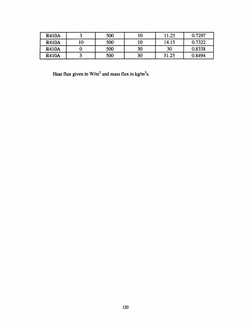
R410A 3 500 10 11.25 0.7297 R410A 10 500 10 14.15 0.7322 R410A 0 500 30 30 0.8338 R410A 3 500 30 31.25 0.8494
Heat flux given in W/m2 and mass flux in kglm2s.
120

I
0.8
! ! ! ! I I I I
• I I , · . . I I I I
: ~: : : --_ ........... - ............... -~ ....................................... ~ ......................................... :- ........................................ -:- ................................ -x
~ 0
, I I I I , , ,
I I • I I I • I
• I I I I I I I I I • I
I • • I
().ti ---------------~---------------1---------------i------- --------t---------------• I • I • , , I I I I I I I • • .. . .. . .. .
0.4 ~- ... .......... -.. ------r ----- ... -- ..... _ ... -- -r'" ........ --- --- -_o. .. '"'r-"'-'" -.............. -_ ... -... ~- -- ._ ......... -_ ....... _-
0.2
· : : ~--'------~ . . : : 0 G=75 . .
---------------~---------------~---------------!------- ... · . . · . . · . . · . . · · . . x
• G=200
G=500
iii J o ~~~~~~~~~~~~~~~~~~~~~~ o 20 40 60 80 100
Average Quality
Figure C.I Void fraction vs. average quality with a heat flux of 0 W/m2 using R134a in a 8.93 mm base diameter axially grooved tube. Mass flux (G) given in kglm2s.
c:: o .g .d:: 't:S .... o >
I
0.8
0.6
0.4
0.2
! ! ! ! · · · . · · x c · · · . · · · , • • I
I I I I ~ . . .
-_.............. .................... ... ................................... -.- ........................................ -.- ....................................... '"',_ ................................. -ex : : : :
· . . I I • • r---------- ... -- ... ~--- ...... -- ... --- .. -... ~----------.----!- ... ----- --------:---------------• • • I · . · . , , · . · . · . · --'" _ ....... - ..... -- -_ ... ~ ...... _ ....... -_ .. -_ ..... -~ ...... _ ... _ .... ------.. -:- -_ ..... --_ ... - - - - - - -:- ...... - -- ............... _ ... --, , I I
: : : ~----.----~ · . . · . . · . . · . , · . . ~-- ... -......... ---- ... -,------------- ... -,-- ... -- ... ---------~- .. ----· . , · . . · . . · . . · . . · . . · . .
o x
•
G=75 G=200 --
G=500
o ~~~~i~~~~i~~~~i~~~~I~~~~ o 20 40 60 80 100
Average Quality
Figure C.2 Void fraction vs. average quality with a heat flux of 3 W/m2 using Rl34a in a 8.93 mm base diameter axially grooved tube. Mass flux (G) given in kglm2s.
121

1
0.8
0.6
0.4
0.2
! ! 10 ! , : 0 , , " , " , , :x . : : r- ........................... ~ .............................. -:- ................................ -:- ............................... -:- ............................. -, , , , , , , , , , , , , , I I , I
------ .. -.. -.. ----~---------------~----- .. ------- .. -~---------------:------_ ........ _ .. --I • I I . . , , • , , I
I I I I , , , roo ........................... ~ ............................. -~ .............................. -:- .............................. -:- ........................... -
, . . . : : : ~~------~ , , , , , , , , , , , , , , ,
---- .. -.. --------~-- .. ---- .. -.. -----~------------- .. -~-- .. -----, , , , , , , , , , , , ,
o x
G=75
G=2oo
o ~~~~i~~~~i~~~~i~~~~i~~~~ o 20 40 60 80 100
Average Quality
Figure C.3 Void fraction vs. average quality with a heat flux of 10 W/m2 using Rl34a in 8.93 mm base diameter axially grooved tube. Mass flux (G) given in kglm2s.
1
0.8
0.6
0.4
0.2
! ! ! , , , , , , , , I I I I I I I I
: .: : : -- ........................... r ............ 0 .......... --t ............................. -t .............................. -~- .......................... -
• ~ I t I I
--------- .. -----~---- .. ----------~------ .. ----- .. --!----- .. --- .... -.. --~------ .. --------I • • I
• • I I I • • I I • I I
• • , I I • I I
• I • I I • I •
~ .... -_ .. ---_ .... -.. -~ _ .. _ ...... --_ .. _ ...... -~ _ ........ _ .. -_ .. -_ ...... :- -............................... :- .......... -.............. -I • , I
: I : ,....-------,1 , , , , , , , , , , , , , --- .......... -- .. ----~---- .. - .. - .. - .......... ~-- ........ -- .. --- .. --! .. -------
, , , , , , , , , , , , , , ,
o x
• G=75 G=2oo
G=5oo
iii i o ~~~~~~~~~~~~~~~~~~~~ o 20 40 60 80 100
Average Quality
Figure C.4 Void fraction vs. average quality with a heat flux of 0 W/m2 using R410A in a 8.93 mm base diameter axially grooved tube. Mass flux (G) given in kglm2s.
122

1
0.8
0.6
0.4
0.2
o
! ! ! · . . ! x U' · . . · . . · . . : _ 0: : : : x: : : r''' ........................ -po ................................ -.- ............................... -,- ............................... -'''' ......................... --
• x • I I I 0: : : : · . . · . . · . . , • I I
• I • I
• I I , ------ .. --------~--- .. --- ....... --- .. -~---------- ... ----!-- .. --- .. .. _ .. _----!----------_ .. _--I • I I I , I I
• f I I I I I I I I • I .. . .. . .. .
t--- ......................... --~ ... - .. -_ .................. - -r"""-"""" -- ............ ~ .. -_ .. -- ................. -: ............... -- ......... --I • , I
: . : ~--.------~ · . · . · · . · . . ---------------~ .. --------------~---------------!------ ....
o
· . . · . . · . . · · i
20
· . . · . i i
40 60 Average Quality
o G=75 x G=200
• G=500
I
80 100
Figure C.S Void fraction vs. average quality with a heat flux of 3 W/m2 using R410A in a 8.93 mm base diameter axially grooved tube. Mass flux (G) given in kg/m2s.
= o . .= ~ ~ "0 .... '0 >
1
0.8
0.6
0.4
0.2
o
! ! ! ! • I I I : : 0: : : x : I
~- .......................... -~ .............................. _Q ... ~ ................................ : ..................................... : ................................ -~ : : :
• I I I I · . · . · . · . • I I I
---------------~----------- .. ---~------------ .. --:---- .... ---------;---------------I I I I · . · . · . · . · . · . · . r--- .. - ---....... _ .......... ~ --.......... - ......... - ...... ~ ....... - ........................ ~ .. ---................ ---:- .... - - ... - -........... --• • • I
: I : ._--"-------i · . , . · . . ' . · , · . . ---- .. - .. - .. - .. -- .. -~---- .. ----- ... -- ...... ~- ... --- ..... ----- ... - .. !---- .. -- ... · . . · . . · . . · . . · . . · . . i i i
o 20 40 60 Average Quality
o x
• I
80
G=75
G=200
G=500
100
Figure C.6 Void fraction vs. average quality with a heat flux of 10 W/m2 using R410A in a 8.93 mm base diameter axially grooved tube. Mass flux (G) given in kg/m2s.
123

1
0.8
0.6
0.4
0.2
o o
: ! • x· : . . : 0: : :
.................................... ~- .................................... :.. ........................................... : .......................................... -:- ................................... .. • I I I I I I I I , I I , I I I
a : · · . · . -------------,---------------~---------------~---------------~-------------• I I I I I I ,
• I I I , , • I
I I f I I • I I I • I I
I I I I I I I I I I I ,
...................................... r .................................... -r ....................................... -,- ......................................... -,- ................................ ...
-------------,---------------,---------------T------· . . · . . · . . · . . · · · 20 40 60
Average Quality
o Q=O
x Q=3
• Q=lO
80 100
Figure C.7 Void fraction vs. average quality with a mass flux of 75 kglm2s using RI34a in a 8.93 mm base diameter axially grooved tube. Heat flux (Q) in W/m2•
c: o . .::: g tt !"O .... o >
1
0.8
0.6
0.4
0.2
o
oX :. . . . ....................................... \. .................................... -.- .................................................................................. -, ................................. ... X : : : :
0: : : : , • • I
• • I I I • • •
: ' : ' o I : I :
-------------~- ...... ------------,---------------~---------------T-------------· . · . · . · . · . · . · - - - _ .. - - ... - - - - - ... ~ - - - ..... - .. - - - .. - ..... -:- .. - _ ...... - ... - - ...... - -!. .... - ... - - - - - .... - - - -:- - ... - ..... - ........... - ..... · ' . ! : I · . · . · . · . · . · . · . .. -- .. -- ... -- ... ---~ ..... ---- .. -- .. - .......... : ... -- ... ---- ..... -----! ............
· . · . · : · · ·
o x
•
Q=O
Q=3
Q=1O
20 40 60 80
Average Quality
100
Figure C.8 Void fraction vs. average quality with a mass flux of 200 kglm2s using RI34a a 8.93 nun base diameter axially grooved tube. Heat flux (Q) in W/m2•
124

1 ! ! ! ! , , , , , , , , · · · , · · . · · · . · 0.8 I , I I
~ ............... ~ .................. ~ ................................... ...... -:-- ........................................ -:- .......................................... -: ....................................... -• I I I
o • I • I
0.6 -- ...... -... ---- ......... --1----- ...... -...... -...... --1------ ..................... -... t---- ......... -- ... --- ...... f-- .................. --- ...... --I I • I I , • I , I I I I • I I I I , •
I I I I I I , •
0.4 ~ ................................. "'t ...................................... "'r"'''''''''''''''''''''''''''''''''''' -r ...................................... -~- ................................ --
0.2
o
· . . · . . · . . · : : 0 G=75 · , · . . ------ ... -...... --- ...... ~----- ...... ---- ......... -~------- ... ---- ... --~ ... ------ ...
o
· · i 20
· . · . · . · . · ,
i
40
. ,
i
60
Average Quality
x G=2oo
80 100
Figure C.9 Void fraction vs. average quality with a mass flux of 500 kglm2s using R134a in a 8.93 mm base diameter axially grooved tube. Heat flux (Q) in W/m2•
1
0.8
§ .... -~ d::
0.6
'0 .... . ~ 0.4
0.2
! · · · ! ,
, . ! · e:
· x: : I
X'
• .• ' I I ~ ......................................... ~ ........................................ ~ ...................................... -!.. .......... ............................. -! ..................................... --
: 0: : : x:: : . . . . , .
o : I I
----- ... ----- ... -... -~ ... ------------- ... ~-- ...... --- ... -- ... -... --~- .. -... -- ... ---_ ...... _-;---------------I I • I , .. · .. · .. · . · . , . · . I , , , r-- '"' --.......... ,",'" --'"' .. ~ ... -........... _ ........... -...... '"'!"' ................... - '"' ..... - - - -:- ....................................... -:'"' ... - - ....... - ............. _-, t , I : : : r---.------~ · . , · , , · . . · . . , . . · . . ~ ... - .. - ...... '"' ...... ----~ ............. --------- ... ~-- ... ---- ... -- ... - ..... -! ... -- ... --- ... · . · , · . · . · . , .
o 20 40 60 Average Quality
o x
•
80
Q=O
Q=3 Q=10
-
100
Figure C.1O Void fraction vs. average quality with a mass flux of75 kglm2s using R410A in a 8.93 mm base diameter axially grooved tube. Heat flux (Q) in W/m2•
125

c:: o . .::: ~
d:: '0 ..... o >
1
0.8
0.6
0.4
0.2
o o
. . • • •
oX
I X I I I
................................... ~ ............ .. G- .......... -~ ............................ .... :.. .............................. -: ............................... .. ~ : I : .. .
X : : o ~ : · . ---- .... -- ........ -~--- .... -.... ----- .. -,-- .. -.. -- .... ------T----- .. -.. .. --- .... -T"' .... ---- ........... ..
I • • • ............................. po ......................... .... -.., ............................... - .................................. -,- ........................... ..
I , • I , I , I
: : : -------· . . · . . · . . · . . · . . · . -_ .............. ----, ...... _------_ .... _-,---_ .... _ ........ __ .... y-_ .... ----. . . · . · . · .
20 40 60 Average Quality
o X
•
80
Q=O
Q=3
Q=lO
100
Figure C.ll Void fraction vs. average quality with a mass flux of 200 kg/m2s using R410A in a 8.93 mm base diameter axially grooved tube. Heat flux (Q) in W/m2•
1
0.8
0.6
0.4
0.2
o
! ! ! ! It. I · . · . .
I I I I · . : (j<: : :
~- ............................. ~ ............................. -;- ............................... -: .................................. -:"' ............................. -I I • , cS· . . . . , I I I .. . .. . .. . · . I I , I
I I I I ------- .. -- .. --- .. ~-- .. - .... --- .. --- .. -~--- .... - .. --------~ .. - .. ---- ...... _----!"' .......... _- .......... --I I I I · .. · .. · .. · .. · .. · .. · .. , , I I 1---- - ..... - -- - -_ ......... :- ........ - ............... - ............... i ......... - - ......... -- .............. : ...... _ .............. -- ................. :- ............ - - ................ -I I , ,
: : : ~~'------~ · . . · . · . · . ~ .................... -- ....... -~ ..... -...... -- .. -..... -......... ~ ............................................ ! .................... ...
· . . · . . · . . · . · . · . i i i
o 20 40 60 Average Quality
o X
• I
80
Q=O Q=3 1-
Q=lO
100
Figure C.12 Void fraction vs. average quality with a mass flux of 500 kg/m2s using R410A in a 8.93 mm base diameter axially grooved tube. Heat flux (Q) in W/m2•
126

1
0.95 0 R134aG=75
0.9 0 R134aG=200 <> R134aG=500
---;- -------- -;-- -------. --- ------;- --fB--I , I I
I I I I I I I I
s:: 0.85 0 .,:::
~ ~ 0.8 '0 .... 0 > 0.75
• R41OAG=75
• R41OAG=200
•
I I I I ---:----- ----: --- ------ :-- ----t"! ------: ! : 0 -. 0 --; --------+ ---------j- ---.. i\ -------___ . ___ . ___ . _.0;1: : <? :
I I I I I I I .............. : .................. : .................. : .................. : .................. ! .... ii" .... ~ : -8- .......... ; ............ .. I I I I I I I
I I • I I I I
0.7 I I I I I I I -- .. -_ .. --~ -_ .. --- ---: -- -_ .. -_ .. -~ ........ -_ .. --~ -_ .. -.. -- -:* ...... -t:t;- .. -_ .. -- .... -;- -- .. -- .... I I I '. I , I : : : .: : : :
0.65
0.6
0.6 0.65 0.7 0.75 0.8 0.85 0.9 0.95 1
Homogenous Correlation
Figure C.13 Void fraction vs. homogenous correlation for 8.93 mm base diameter helically grooved tube using R134a and R41OA. Mass Flux (G) given in kglm2s.
1
0.9 o D=7.25 mm R134a
o D=7.25mmR41OA
s:: 0.8 0 .... ..... ~ ~ 0.7 '0 .... 0 '>
• D=8.89 mm Rl34a ; • ---------- : ------------~o- 0---.: D=8.89 ~m R41OA: 1 ~ i~ 0
------ -----;- --- ---------: -- ----------: ------- -0 -tt-·--- [JI- -if----------l ~ ~ • ~ I I I •
I I I I
0.6 -_ .. -_ .. --- .... ~ ............... _--- .. :- ............ -......... d- -- .... -.. -- ........ : .... -- ................ : ........ -- ........ .. I I I I I I I I I •
I I , I •
I I I I I I I I I I .
0.5
0.4
0.4 0.5 0.6 0.7 0.8 0.9 1
Homogenous Correlation
Figure C.14 Void fraction vs. homogenous correlation for 7.25 mm and 8.93 mm base diameter helically grooved tubes.
127

1 o Rl34aG=75
0.95 o Rl34aG=200 • I • I
0.9 c: 0
',c 0.85 ~ ~ "t:S 0.8 .... 0 >
: : : : 0 <> Rl34a G=500 ---t---------t--------: ---------:-~-----• R410A G=75 : : : cp
: : : -- 0: "---i----"'''- --- I .... ---+ .. :--~- .. t,;-: ........ -----
• R410A G=200 1. ~~ 1 . .. ................ ~- ......... - .. ~- ................. ~ .............. ..
<> p • 1 1 I • I I I
0.75 _______ ~ _________ ~ .. ____ .. ___ _ _______ ~ _________ ~ _________ ~ _________ L ______ _
~ .i I .0 : : ~
0.7
0.65
0.6
0.6 0.65 0.7 0.75 0.8 0.85 0.9 0.95 1
Rigot Correlation
Figure C.15 Void fraction vs. Rigot correlation for 8.93 mm base diameter helically grooved tube using Rl34a and R410A Mass Flux (G) given in kglm2s.
1
0.9
0.8
0.7
0.6
0.5
0.4
· -----------~----------- .. -----------· ·
0.5 0.6 0.7
o D=7.25mm RI34a --
o D=7.25mm R410A
• D=8.93mm RI34a --
• D=8.93mm R410A
0.8 0.9
Rigot Correlation
1
Figure C.16 Void fraction vs. Rigot correlation for 7.25 mm and 8.93 mm base diameter helically grooved tubes.
128

I
0.9
= 0.8 0 ..... +-'
~ tt 0.7 '0 ..... 0 >
0.6
0.5
0.4
0.4
I I I , ___________ ~---- ________ ~ ____________ 4 ____________ ~ ___ ________ _
: . ~: : * : I I • I. I
--- -------- : ----------- -:- ------0 -- -3" ------------ -. ---------: -----------: : : jl : : • 1 • 0 ~
- -- - -- --<7 -:- - -- -+- --- ---: -.- -- --0--- - : ---- ----
01 I 1 o
_____ .......... __ , ____________ I ... ___________ : _______ _
0.5 0.6
o
o
0.7
Zivi Correlation
0 R134aG=75 0 R134aG=200
<> R134aG=500
• R41OAG=75
• R41OAG=200
• R41OAG=500
0.8 0.9 1
Figure C.17 Void fraction vs. Zivi correlation for 8.93 mm base diameter helically grooved tube using RI34a and R41OA. Mass Flux (G) given in kglm2s.
I
0.9
0.8 = 0 ..... +-'
~ 0.7 tt '0 .....
0.6 0 ;>
0.5
0.4
0.3
0.3
o
: : : : 0: .:::J: ................. .. :- ...................... ! ....................... -;- .................. i ...... (3)- ...... :.. .. ............ -:- .............. ...
1 1. 1 Citli 0 1 1 ------ ---r- --- -= -1-- --; -----r------:--- --- --- --: ---- -----r -----_________ ~ __________ ~ __________ ___________ ~ __________ A ___________ • ________ _
o 0 0
o 0 0 o 0 0
0: : :
0.4 0.5 0.6
o o
D=7.25mm R134a
D=7.25mm R410A
• D=8.93mm R134a
D=8.93mm R410A
0.7 0.8 0.9
Zivi Correlation
1
Figure C.18 Void fraction vs. Zivi correlation for 7.25 mm and 8.93 mm base diameter helically grooved tubes.
129

l:: 0 .~
~ ~ "0 ..... 0 >
1
0.95
0.9
0.85
0.8
0.75
0.7
0.65
o o o
-R134aG=75 · . · . .
----~--·------:---------:---------:------ti R134a G=200 : . . r. : R134a G=500 : : : <..T' 0
-- - - -:- - - - -- - -- -:- - - -- - -- - '- - - - - -0. - -:- - - - -- --R410A G=75 : : : ~
• R410A G=200 --- -J- ------ --: ------ -~ .-- ----~- --- ---· . .. . : 0: .- 0: : : 0: :
.' -- -- : -- ------ -:-.0.- -1-:- ---------:- -------:: <>::: I I I I I I
I I I : I • •
................. -: .................... ~ .............................. ..:..0 .. ~ ..... -0 ......... ~ ................... ; ..................... ~ ............. .. : : : -, : : : I I I ' I I I
: : : : : : : ................. ~.... ........ .... : ............. -~ ... - ... .Q. -~ ................. -!- ................ -:- .................. -:- ............... ..
: ' t I
• R41OAG=500
0.6 0.65 0.7 0.75 0.8 0.85 0.9 0.95 Ahrens-Thorn Correlation
1
Figure C.19 Void fraction vs. Ahrens-Thorn correlation for 8.93 mm base diameter helically grooved tube using Rl34a and R41OA. Mass Flux (G) given in kglm2s.
1
0.9
l:: 0.8 0 . ~ ~ ~ "0 ..... 0.7 0 >
0.6
0.5
0.4
0.4
I I I I I
: : : : : 0
···········f············f············l ............ j ........... ~~. : : ; : -~~
-----------:------------;-------------;----------- ~-CJ---)1I-lIts----------. . . rl· 8 . : : : : _ 0: I I I I I
------ --- --l- --- --- ------ ~ --- -- --- --- :0--.--~ i-l- --Q ---- --- -l-- --- ------: : 0 rr- : : : : :- : : . . .
· ----------- -----0---- :-------------;-------· . · . · . · .
o o
D=7.25mm R134a
D=7.25mm R410A · . - D=8.89 mm R134a
• D=8.89 mm R410A
0.5 0.6 0.7 0.8 0.9 I
Ahrens-Thorn Correlation
Figure C.20 Void fraction vs. Ahrens-Thorn correlation for 7.25 mm and 8.93 mm base diameter helically grooved tubes.
130

1
0.9
0.8
0.7
0.6
0.5
0.5
· . . --------------r---------------~---------------r------- ------· . . · . · . · · · · · · . -------------1-------------~~----~------ .. :---------------t-------------
: : . : ..... --_._-----. I n~ :. : •• ~ I .. . . -----------0--: -----.------- : ---------------:---
O · . . I ~ ~ · · · ------._._--. ---------------~---------------.---· . . · . . · . . · . . · . . · . . · . . · . .
0.6 0.7 0.8
Baroczy Correlation
a o o
R134aG=75 R134aG=200 R134aG=500 R410AG=75
• R410A G=200 • R410AG=500
0.9 1
Figure C.21 Void fraction vs. Baroczy correlation for 8.93 mm base diameter helically grooved tube using R134a and R41OA. Mass Flux (G) given in kglm2s.
1
0.9
s:: 0.8 0 .:;:
~ ~ "0 .... 0.7 0 >
0.6
0.5
0.4
0.4
: : : Q ~: -----------~------------~----------lIf.L----E) -- ------------~-----------
: : ~~ : ! : II ~. I ~ ---. ------+ ---------e-~ ---ii-- -- : ---- --- --- --1- -- --- -.- ----[--. ----- ---1 .. ~ : : :
----------- .------------ .-------------:- a D=7.25mm Rl34a
o
0.5
· . : : 0 D=7.25mm R410A · . · .
•
0.6 0.7
D=8.93mm Rl34a D=8.93mm R410A
0.8 0.9
Baroczy Correlation
1
Figure C.22 Void fraction vs. Baroczy correlation for 7.25 mm and 8.93 mm base diameter helically grooved tubes.
131

§ ..... ..... ~ ~ "0 ..... o >
1
0.9
0.8
0.7
0.6
0.5
0.5
. I I I I ... _ .. -_ .. ---_ .... --~ -- .. -- .. -_ .. -_ .. -- ... ~- ... -- ...... -... -_ .. -_ ...... :-€: .. -_ .. -_ .. -_ .... : .. -_ ......... -_ ........... : : : 0 :
: : " 0 : : :. 0 :
i i o.~ i -------------: ---------------: -----<i -.,:: -.- --. ---------------: -------------
I • '!:1' I I : : . : . ..0 -- --- --- --- ---~ -- --~- -.-- --- -: ----- -- --- ---. .
:IJI •
0.6 0.7 0.8
o o <>
•
R134aG=75
R134aG=200
R134aG=500
R41OAG=75
• R410A G=200
• R41OAG=500
0.9
Hugbmark Correlation
1
Figure C.23 Void fraction vs. Hughmark correlation for 8.93 mm base diameter helically grooved tube using R134a and R410A. Mass Flux (G) given in kglm2s.
1
0.9
I:: 0
0.8 ..... ..... ~ ~ "0 .....
. ~ 0.7 0 D=7.25mm R134a 0 D=7.25mm R410A
0.6 • D=8.93mm R134a
• D=8.93mm R410A
0.5 0.6 0.7 0.8 0.9 1 Hugbmark Correlation
Figure C.24 Void fraction vs. Hughmark correlation for 7.25 mm and 8.93 mm base diameter helically grooved tubes.
132

I
0.9
c:: 0.8 0 .... ... ~ ~
0.7 oe .... 0 >
0.6
0.5
, ,
: : :". -........ : ........................ -:.. .. .. .. .. .. .. .. .. .. .... :- .................. it : : :., : : 0: , 'i' ... ··l············ ~ iii······· ~ ....... . : 0: 0 : : :..:
L.-_~ _____ ......... i.···;·~·i·o··········(········· lIP. ' , , , , , , , , , ,
....................... :- .....•..... : ....•....... : ............ ~ .......... . : I I t
: 0 0:, : : : :: ------------~------------~------------~-------------~- ---------
: . " : :: : :: , "
0 G=75 R134a
0 G=200R134a
0 G=500R134a
• G=75R41OA
• G=200R410A
• G=500R41OA
0.4
0.4 0.5 0.6 0.7 0.8 0.9 I
Graham Correlation
Figure C.25 Void fraction vs. Graham's condenser correlation for 8.93 mm base diameter helically grooved tube using R134a and R41OA. Mass Flux (G) given in kglm2s.
I
o D=7.26mm R134a 0.9 o D=7.26mm R410A
• D=8.93mm R134a
c:: 0.8 • D=8.93mm R410A 0 . .= ~ ~ 0.7 -----------~------------~---------- .. , , oe .... , , , ,
~ 0.6
, , , , , 0 '
........... ; ............ ; ... G .•.... + .. o •....... ~ ............ ~ .......... . : I 0: : : .. ~ : : I I I I
0.5 ............ ~ .... ii·· G -1-· ......... -1-··········· -1-·········· I I I I
I I I I • I I I
0.4
0.4 0.5 0.6 0.7 0.8 0.9 1
Graham Correlation
Figure C.26 Void fraction vs. Graham's condenser correlation for 7.25 mm and 8.93 mm base diameter helically grooved tubes.
133

AppendixD
Conclusion Plots
These plots correspond to Chapter 8 in which a number of correlations are
presented to accurately predict the data.
134

c:: o • .:= ~ ~ "t:) .... o :>
1
0.9
0.8
0.7
0.6
eel ~ ~ 0
------------------------j-------;,--~-tS<----------------------
- -- ------- --- ----- ---0 ~ -Cb :? _01_ -~ ---------.l. -----------------------o •• a~e:> • ! • 0'. : •• • -----------E)---If-·---~--------------------------~------------------------
• : 0 R134a . : : • R410A
---.- --- --- --- --- --- ---: -- --- --- --- ------ ------'-"------• • · ·
0.5
0.001 0.01 0.1 FtiG
1
Figure D.1 Void fraction vs. FtiG for smooth tube showing refrigerant effects.
1 · ate 0.9
0.8
0.7
: : . ________________________ : _______ ;;_~~-:S<--------------- ______ _
--- ---- --- -- --- --- ---e ~ -C4 :?-"J --~ --------- -~- -------- --- ---- --- -- ---~ 0 .
o· 01:" . • a •• • -----------E)---~-.---:--------------------------:------------------------
•• 0 D=4.26mm
0.6 ---~- --- --- --- --- --- --- ~ -- --- --- --- ---- -- -__ ..... ~.~-D-=6-.-12-m-m---
0.5
0.001 0.01 0.1
FtiG
1
Figure D.2 Void fraction vs. FtiG for smooth tube showing diameter effects_
135

c 0 ..... ..... g
rot '1:J ..... 0 >
1
0.9
0.8
0.7
: : ~~o
i ~: •• ~ · . . ---------- -------:------------------ -;-o. - -0-- - -- - -: -- - -- - -- - -- -- - - --· . . · . . · . . : ~ : ------------------~ ------------~~-r. ------------------i- -----------------: O~: : · . . · . .
-----------------~ ------~- • -------j -------------------; -----------------...:a. . I'" I I :. .: : :., : :
0.6 ................................... .. :w- ....................... ............. :- ....................................... -;- .................................. .. · . · . o R134a
0.5 ................................ • ~ ........................................... ~ ...................... .. • R410A
0.4
10-5 0.0001
· · ·
0.001
Ft*D/G2I3
0.01 0.1
Figure D.3 Void fraction vs. Ft*D/G2/3 for axially grooved tube showing refrigerant effects.
c o ..... .....
~ '1:J ..... '0
>
0.9
0.8
0.7
1 : : ~.~.
; ~: o.~ --- --- ------- -- --~--- ---- -- --- ------- j-•• - -0- - -- - -- i -- --- --- --- ------· . . · . . · . . : ~ : -- ---------- -- --- -i --------~~--'--{ ; ------- --------- --!- ------ ------ -----I ;t:6 I I · . .
-----------------~-----:~4i?-------~-------------------!-----------------I l1r" I I
:. <it: : '0 r::l.. • • I .... • I
0.6 ... -.. -- ......... -_ .............. -:'0- ...... -_ .. -.................. --:- -..... _-o D=7.25 mm
0.5 • D=8.89mm · . .. .... .. .. ... .. .. .. ... .. ... .. .. .. G~ ......................................... ~ ........... .. : : ~----~-------· . · . · . · .
0.4 ~~~~~UL __ ~~-W~~~~~~~ __ ~~~~
10-5 0.0001 0.001
Ft*D/G2I3
0.01 0.1
Figure D.4 Void fraction vs. Ft*D/G213 for axially grooved tube showing diameter effects.
136
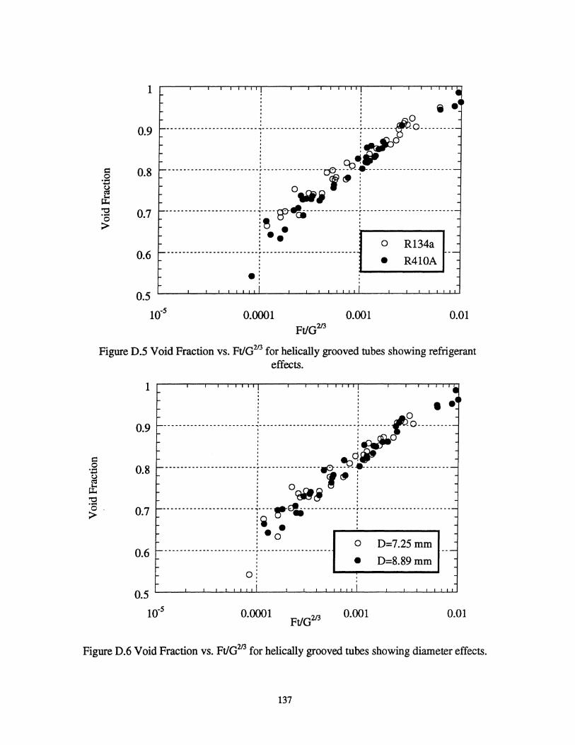
= o .p
~ tt 'tj ....
= o .... .... ~ tt 'tj .... o >
1
0.9
0.8
0.7
0.6
, , ~ . ------------------------i--------------------------~JI------- ~()---------, , , , , , , , , ,
: ~ .. , n..: ,F ------------------------t ----------------,-; r ----------------------l ()tili l
-----------·------------~-~--~~--------------t-------- ----------------'0 ' :. r'----------~ : .. , ,
------------------------r-------------------------. . . :
()
• R134a
R410A
0.5 ~--~~~~~~--~~~~~~--~~~~~~
10-5 0.0001 0.001 0.01 FtlG213
Figure 0.5 Void Fraction vs. FtlG2/3 for helically grooved tubes showing refrigerant effects.
. , .. 0.9
0.8
________________________ j __________________________ [~ClCl ________ _ 1 eaqji
------------------------1----------------~-~-r-------- --------------
l ()~§ 1 o. 0.7 ------------------------~-~--~~--------------~------------------------> 'w ' :. ~~:-----------:·0
: 0 D=7.25mm 0.6 ------------------------r-------------------,
: • D=8.89mm 0: ,
0.5 L--__ ..I..-~..J.._J.....L...J.....L..I-'--__ ..J.._~__'_..J.....L..J._L..I....L_ __ __'____L__L.. ........ L.....L...I...L.J
10-5 0.0001 0.001 0.01
Figure 0.6 Void Fraction vs. FtlG213 for helically grooved tubes showing diameter effects.
137