Technical Report NetApp E-Series Solution for Hadoop Overview, Design, Best Practices, and Performance Faiz Abidi, NetApp March 2018 | TR-3969 Abstract There has been an exponential growth in data over the past decade, and analyzing huge amounts of data within a reasonable time can be a challenge. Apache Hadoop is an open- source tool that can help your organization quickly mine big data and extract meaningful patterns from it. A core component of the Apache Hadoop project is the Hadoop Distributed File System (HDFS), which stores data and provides access to servers for data analysis. NetApp ® storage systems can help with this aspect because they improve throughput and are reliable and easily scalable. This report discusses a brief overview of the Apache Hadoop project, along with some best practices and performance testing with the NetApp E- Series storage system.

Welcome message from author
This document is posted to help you gain knowledge. Please leave a comment to let me know what you think about it! Share it to your friends and learn new things together.
Transcript
Technical Report
NetApp E-Series Solution for Hadoop Overview, Design, Best Practices, and Performance
Faiz Abidi, NetApp
March 2018 | TR-3969
Abstract
There has been an exponential growth in data over the past decade, and analyzing huge
amounts of data within a reasonable time can be a challenge. Apache Hadoop is an open-
source tool that can help your organization quickly mine big data and extract meaningful
patterns from it. A core component of the Apache Hadoop project is the Hadoop Distributed
File System (HDFS), which stores data and provides access to servers for data analysis.
NetApp® storage systems can help with this aspect because they improve throughput and
are reliable and easily scalable. This report discusses a brief overview of the Apache
Hadoop project, along with some best practices and performance testing with the NetApp E-
Series storage system.
2 NetApp E-Series Solution for Hadoop © 2018 NetApp, Inc. All Rights Reserved.
TABLE OF CONTENTS
1 Introduction ................................................................................................................................. 4
1.1 Big Data ............................................................................................................................................... 4
1.2 Hadoop Overview ................................................................................................................................ 4
2 NetApp E-Series Overview ........................................................................................................ 5
2.1 E-Series Hardware Overview ............................................................................................................... 5
2.2 SANtricity Software .............................................................................................................................. 6
2.3 Performance and Capacity................................................................................................................. 11
3 Hadoop Enterprise Solution with NetApp .............................................................................. 13
3.1 Data Locality and Its Insignificance for Hadoop ................................................................................. 13
3.2 NetApp E-Series ................................................................................................................................ 13
3.3 Hadoop Replication Factor and Total Cost of Ownership .................................................................. 13
3.4 Enterprise-Class Data Protection ....................................................................................................... 14
3.5 Enterprise-Level Scalability and Flexibility ......................................................................................... 14
3.6 Hortonworks and Cloudera Certified .................................................................................................. 14
3.7 Easy to Deploy and to Use................................................................................................................. 14
4 Experimental Design and Setup .............................................................................................. 14
4.1 Architectural Pipeline and Hardware Details ...................................................................................... 14
4.2 Effect of HDFS Block Size, Network Bandwidth, and Replication Factor ........................................... 15
4.3 Hadoop Tuning .................................................................................................................................. 16
4.4 Rack Awareness ................................................................................................................................ 18
4.5 Operating System Tuning .................................................................................................................. 18
4.6 E-Series Setup ................................................................................................................................... 19
4.7 NetApp In-Place Analytics Module ..................................................................................................... 20
5 Results ....................................................................................................................................... 20
6 Hadoop Sizing ........................................................................................................................... 21
7 Conclusion ................................................................................................................................ 22
8 Future Work ............................................................................................................................... 22
3 NetApp E-Series Solution for Hadoop © 2018 NetApp, Inc. All Rights Reserved.
Acknowledgments .......................................................................................................................... 22
References ....................................................................................................................................... 22
Appendix .......................................................................................................................................... 23
Version History ............................................................................................................................... 23
LIST OF TABLES
Table 1) Hadoop components. ................................................................................................................................ 5
Table 2) E5700 controller shelf and drive shelf models. .......................................................................................... 5
Table 3) Available drive capacities for E5700. ....................................................................................................... 13
Table 4) Reserved memory recommendations. ..................................................................................................... 17
Table 5) Container size recommendations. ........................................................................................................... 17
Table 6) YARN and MapReduce configuration values. ......................................................................................... 17
Table 7) Operating system parameters that must be configured. .......................................................................... 18
Table 8) Results obtained by using 8 nodes and one E5700 storage array with 96 drives. .................................. 20
LIST OF FIGURES
Figure 1) MapReduce architecture. ......................................................................................................................... 4
Figure 2) E5700 drive shelf options. ........................................................................................................................ 6
Figure 3) Components of a pool created by the DDP feature. ................................................................................. 7
Figure 4) DDP pool drive failure. ............................................................................................................................. 8
Figure 5) Technical components of NetApp E-Series FDE feature with an internally managed security key. ......... 9
Figure 6) Technical components of NetApp E-Series FDE feature with an externally managed security key. ...... 10
Figure 7) Write-heavy workload expected system performance on E5700. .......................................................... 12
Figure 8) Read-heavy workload expected system performance on E5700. .......................................................... 12
Figure 9) Overview of the experimental setup. ...................................................................................................... 15
Figure 10) Read/write test with replication factor (RF) 2 and RF 3. ....................................................................... 16
Figure 11) Python script to calculate Hadoop cluster configuration. ...................................................................... 18
Figure 12) E5700 results. ...................................................................................................................................... 23
4 NetApp E-Series Solution for Hadoop © 2018 NetApp, Inc. All Rights Reserved.
1 Introduction
This report briefly discusses the various components of the Hadoop ecosystem. It also presents an
overview of the E-Series solution by NetApp, why you should choose NetApp for Hadoop, and how
the E-Series storage system performs in terms of throughput and time. It also includes best practices
for configuring a Hadoop cluster and the kernel-level tuning to extract optimal performance.
1.1 Big Data
Data has been growing at a speed that no one could have predicted 10 years ago. The constant influx
of data that’s produced by technologies such as CCTV cameras, driverless cars, online banking,
credit card transactions, online shopping, machine learning, and social networking must be stored
somewhere. In 2013, it was estimated that 90% of the world’s data had been generated over the past
two years [1]. With such large amounts of data being generated, it becomes imperative to analyze this
data and to establish the hidden patterns and behavior. The mining of big data for meaningful insights
has several use cases in different industries. Just one example is e-commerce companies such as
Amazon who can use this information to tailor advertisements for a specific audience.
1.2 Hadoop Overview
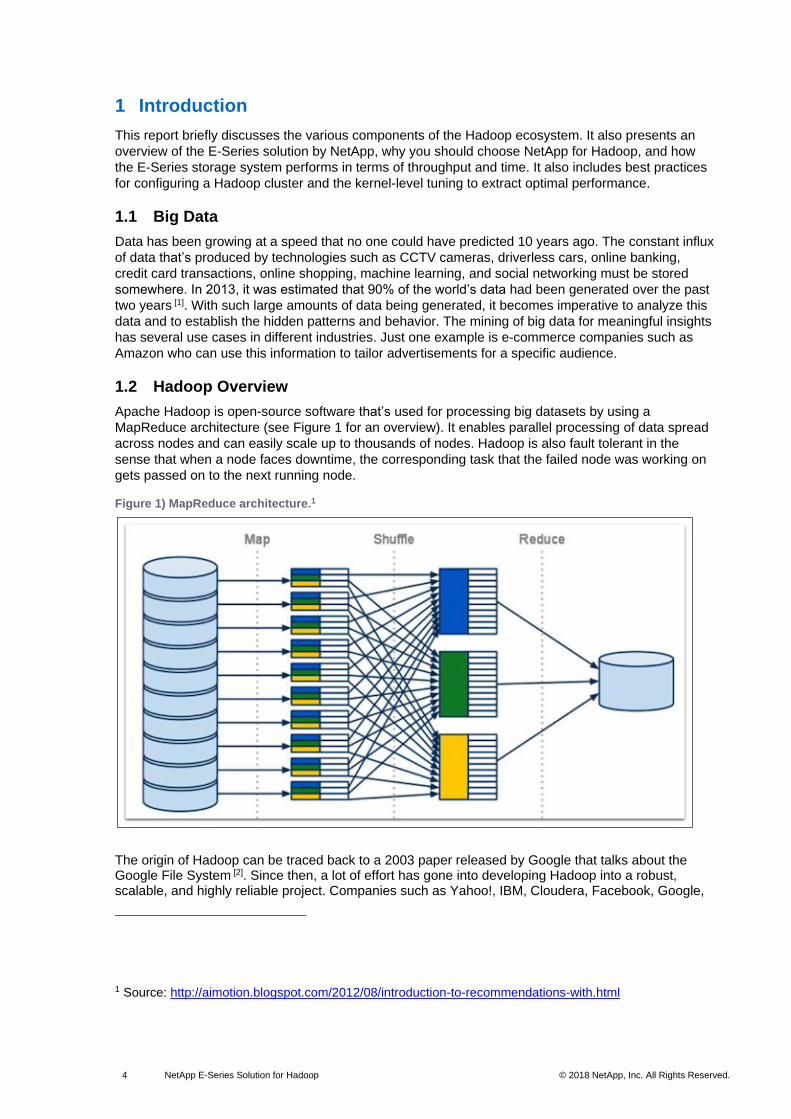
Apache Hadoop is open-source software that’s used for processing big datasets by using a
MapReduce architecture (see Figure 1 for an overview). It enables parallel processing of data spread
across nodes and can easily scale up to thousands of nodes. Hadoop is also fault tolerant in the
sense that when a node faces downtime, the corresponding task that the failed node was working on
gets passed on to the next running node.
Figure 1) MapReduce architecture.1
The origin of Hadoop can be traced back to a 2003 paper released by Google that talks about the Google File System [2]. Since then, a lot of effort has gone into developing Hadoop into a robust, scalable, and highly reliable project. Companies such as Yahoo!, IBM, Cloudera, Facebook, Google,
1 Source: http://aimotion.blogspot.com/2012/08/introduction-to-recommendations-with.html
5 NetApp E-Series Solution for Hadoop © 2018 NetApp, Inc. All Rights Reserved.
and others have been constantly contributing to the project. Table 1 discusses the four main projects (components) of Apache Hadoop. There are also other related projects, such as Spark, HBase, and Mahout, and each project has its own use case.
Table 1) Hadoop components.2
Component Description
Hadoop Common The common utilities that support the other Hadoop modules
Hadoop Distributed File System (HDFS) A distributed file system that provides high-throughput access to application data
Hadoop YARN A framework for job scheduling and cluster resource management
Hadoop MapReduce A YARN-based system for parallel processing of large datasets
2 NetApp E-Series Overview
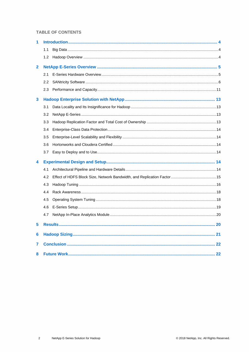
The industry-leading E-Series E5700 storage system delivers high IOPS and high bandwidth with
consistently low latency to support the demanding performance and capacity needs of science and
technology, simulation modeling, and decision support environments. The E5700 is equally capable of
supporting primary transactional databases, general mixed workloads, and dedicated workloads such
as video analytics in a highly efficient footprint, with extreme simplicity, reliability, and scalability.
E5700 systems provide the following benefits:
• Support for wide-ranging workloads and performance requirements
• Fully redundant I/O paths, advanced protection features, and proactive support monitoring and services for high levels of availability, integrity, and security
• Increased IOPS performance by up to 20% over the previous high-performance generation of E-Series products
• A level of performance, density, and economics that leads the industry
• Interface protocol flexibility to support FC host and iSCSI host workloads simultaneously
• Support for private and public cloud workloads behind virtualizers such as NetApp FlexArray®
software, Veeam Cloud Connect, and NetApp StorageGRID® technology.
2.1 E-Series Hardware Overview
As shown in Table 2, the E5700 is available in two shelf options, which support both HDDs and solid-
state drives (SSDs) to meet a wide range of performance and application requirements.
Table 2) E5700 controller shelf and drive shelf models.
Controller Shelf Model
Drive Shelf Model
Number of Drives
Type of Drives
E5760 DE460C 60 2.5" and 3.5" SAS drives (HDDs and SSDs)
E5724 DE224C 24 2.5" SAS drives (HDDs and SSDs)
2 Source: http://hadoop.apache.org/
6 NetApp E-Series Solution for Hadoop © 2018 NetApp, Inc. All Rights Reserved.
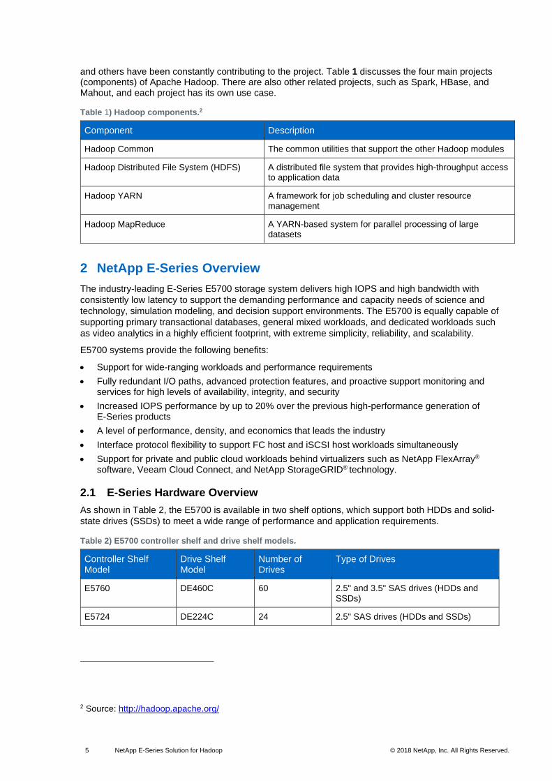
Both shelf options include dual-controller modules, dual power supplies, and dual fan units for
redundancy. The 24-drive shelf has integrated power and fan modules. The shelves are sized to hold
60 drives or 24 drives, as shown in Figure 2.
Figure 2) E5700 drive shelf options.
Each E5700 controller shelf includes two controllers, with each controller providing two Ethernet
management ports for out-of-band management. The system has two 12Gbps (4-lane wide) port SAS
drive expansion ports for redundant drive expansion paths. The E5700 controllers also include two
built-in host ports, which can be configured as either 16Gb FC or 10Gb iSCSI. The following host
interface cards (HICs) can be installed in each controller:
• 4-port 12Gb SAS wide port (SAS-3 connector)
• 4-port 32Gb FC
• 4-port 25Gb iSCSI
• 2-port 100Gb InfiniBand
Note: Both controllers in an E5700 array must be identically configured.
2.2 SANtricity Software
E5700 systems are managed by NetApp SANtricity® System Manager 11.40, which is embedded on
the controller.
To create volume groups on the array, the first step when you configure SANtricity is to assign a
protection level. This assignment is then applied to the disks that are selected to form the volume
group. E5700 storage systems support Dynamic Disk Pools (DDP) technology and RAID levels 0, 1,
5, 6, and 10. We used DDP technology for all the configurations that are described in this document.
To simplify the storage provisioning, NetApp SANtricity provides an automatic configuration feature.
The configuration wizard analyzes the available disk capacity on the array. It then selects disks that
maximize array performance and fault tolerance while meeting capacity requirements, hot spares, and
other criteria that are specified in the wizard.
For more information about SANtricity Storage Manager and SANtricity System Manager, see the
E-Series Systems Documentation Center.
4 5 6 70 1 2 3 12 13 14 158 9 10 11 20 21 22 2316 17 18 19
1200G
B
1200G
B
1200G
B
1200G
B
1200G
B
1200G
B
1200G
B
1200G
B
1200G
B
1200G
B
1200G
B
1200G
B
1200G
B
1200G
B
1200G
B
1200G
B
1200G
B
1200G
B
1200G
B
1200G
B
1200G
B
1200G
B
1200G
B
1200G
B
E57242U -24 drive shelf
Front87 954 621 3 1110 12
Front87 954 621 3 1110 12
Front87 954 621 3 1110 12
Front87 954 621 3 1110 12
Front87 954 621 3 1110 12
11852
10741
9630
11852
10741
9630
11852
10741
9630
11852
10741
9630
11852
10741
9630
E57604U -60 drive shelf
Front View
Front View (open)
Rear ViewX2 2
X2 2
LNK LNK
P1 P2
EXP1 EXP2
LNK LNK0a 0b
LNK LNK0e 0fLNK LNK0c 0d
LNK LNK
P1 P2
EXP1 EXP2
LNK LNK0a 0b
LNK LNK0e 0fLNK LNK0c 0d
A
B
1
2X2 2 X2 2
LNK LNK
P1 P2
EXP1 EXP2
LNK LNK0a 0b
LNK LNK0e 0fLNK LNK0c 0d
LNK LNK
P1 P2
EXP1 EXP2
LNK LNK0a 0b
LNK LNK0e 0fLNK LNK0c 0d
FC/iSCSI (SFP+) base host
interface with 32Gb FC HIC
shown
LNK LNK
EXP1 EXP2
LNK LNK
0a 0b
P1 P2
LNK0c
LNK0d
LNK0e
LNK0f
LNK LNK
EXP1 EXP2
LNK LNK
0a 0b
P1 P2
LNK0c
LNK0d
LNK0e
LNK0f
LNK LNK
EXP1 EXP2
LNK LNK
0a 0b
P1 P2
LNK0c
LNK0d
LNK0e
LNK0f
LNK LNK
EXP1 EXP2
LNK LNK
0a 0b
P1 P2
LNK0c
LNK0d
LNK0e
LNK0f
7 NetApp E-Series Solution for Hadoop © 2018 NetApp, Inc. All Rights Reserved.
Dynamic Storage Functionality
From a management perspective, SANtricity offers several capabilities to ease the burden of storage
management, including the following:
• New volumes can be created and are immediately available for use by connected servers.
• New RAID sets (volume groups) or disk pools can be created at any time from unused disk devices.
• Dynamic volume expansion allows capacity to be added to volumes online as needed.
• To meet any new requirements for capacity or performance, dynamic capacity expansion allows disks to be added to volume groups and to disk pools online.
• If new requirements dictate a change, for example, from RAID 10 to RAID 5, dynamic RAID migration allows the RAID level of a volume group to be modified online.
• Flexible cache block and dynamic segment sizes enable optimized performance tuning based on a particular workload. Both items can also be modified online.
• Online controller firmware upgrades and drive firmware upgrades are possible.
• Path failover and load balancing (if applicable) between the host and the redundant storage controllers in the E5700 are provided. For more information, see the Multipath Drivers Guide.
Dynamic Disk Pools Feature
The Dynamic Disk Pools (DDP) feature dynamically distributes data, spare capacity, and protection
information across a pool of disks. These pools can range in size from a minimum of 11 drives to all
the supported drives in a system. In addition to creating a single pool, storage administrators can opt
to mix traditional volume groups and a pool or even multiple pools, offering greater flexibility.
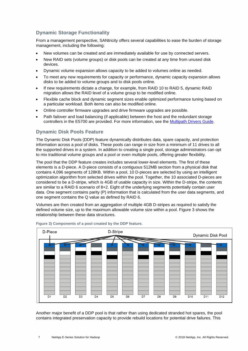
The pool that the DDP feature creates includes several lower-level elements. The first of these
elements is a D-piece. A D-piece consists of a contiguous 512MB section from a physical disk that
contains 4,096 segments of 128KB. Within a pool, 10 D-pieces are selected by using an intelligent
optimization algorithm from selected drives within the pool. Together, the 10 associated D-pieces are
considered to be a D-stripe, which is 4GB of usable capacity in size. Within the D-stripe, the contents
are similar to a RAID 6 scenario of 8+2. Eight of the underlying segments potentially contain user
data. One segment contains parity (P) information that is calculated from the user data segments, and
one segment contains the Q value as defined by RAID 6.
Volumes are then created from an aggregation of multiple 4GB D-stripes as required to satisfy the
defined volume size, up to the maximum allowable volume size within a pool. Figure 3 shows the
relationship between these data structures.
Figure 3) Components of a pool created by the DDP feature.
Another major benefit of a DDP pool is that rather than using dedicated stranded hot spares, the pool
contains integrated preservation capacity to provide rebuild locations for potential drive failures. This

8 NetApp E-Series Solution for Hadoop © 2018 NetApp, Inc. All Rights Reserved.
approach simplifies management, because individual hot spares no longer need to be planned or
managed. The approach also greatly improves the time for rebuilds, if necessary, and enhances
volume performance during a rebuild, as opposed to traditional hot spares.
When a drive in a DDP pool fails, the D-pieces from the failed drive are reconstructed to potentially all
other drives in the pool by using the same mechanism that is normally used by RAID 6. During this
process, an algorithm that is internal to the controller framework verifies that no single drive contains
two D-pieces from the same D-stripe. The individual D-pieces are reconstructed at the lowest
available logical block address (LBA) range on the selected disk.
In Figure 4, disk 6 (D6) is shown to have failed. Subsequently, the D-pieces that previously resided on
that disk are recreated simultaneously across several other drives in the pool. Because multiple disks
participate in the effort, the overall performance impact of this situation is lessened, and the length of
time that is needed to complete the operation is dramatically reduced.
Figure 4) DDP pool drive failure.
When multiple disk failures occur within a DDP pool, to minimize the data availability risk, priority for
reconstruction is given to any D-stripes that are missing two D-pieces. After those critically affected D-
stripes are reconstructed, the remainder of the necessary data is reconstructed.
From a controller resource allocation perspective, there are two user-modifiable reconstruction
priorities within a DDP pool:
• Degraded reconstruction priority is assigned to instances in which only a single D-piece must be rebuilt for the affected D-stripes; the default for this value is high.
• Critical reconstruction priority is assigned to instances in which a D-stripe has two missing D-pieces that need to be rebuilt; the default for this value is highest.
For large pools with two simultaneous disk failures, only a relatively small number of D-stripes are
likely to encounter the critical situation in which two D-pieces must be reconstructed. As discussed
previously, these critical D-pieces are identified and reconstructed initially at the highest priority. This
approach returns the DDP pool to a degraded state quickly so that further drive failures can be
tolerated.
In addition to improving rebuild times and providing superior data protection, DDP technology can also
provide much better performance of the base volume under a failure condition than with traditional
volume groups.
For more information about DDP technology, see TR-4115: SANtricity Dynamic Disk Pools Best
Practices Guide.
9 NetApp E-Series Solution for Hadoop © 2018 NetApp, Inc. All Rights Reserved.
E-Series Data Protection Features
E-Series systems have a reputation for reliability and availability. Many of the data protection features
that are in E-Series systems can be beneficial in a Hadoop environment.
Encrypted Drive Support
E-Series storage systems provide at-rest data encryption through self-encrypting drives. These drives
encrypt data on writes and decrypt data on reads regardless of whether the full disk encryption (FDE)
feature is enabled. Without the FDE enabled, the data is encrypted at rest on the media, but it is
automatically decrypted on a read request.
When the FDE feature is enabled on the storage array, data at rest is protected by locking the drives
from reads or writes unless the correct security key is provided. This process prevents another array
from accessing the data without first importing the appropriate security key file to unlock the drives. It
also prevents any utility or operating system from accessing the data.
SANtricity 11.40 has further enhanced the FDE feature by introducing the capability for you to
manage the FDE security key by using a centralized key management platform. For example, you can
use Gemalto SafeNet KeySecure Enterprise Encryption Key Management, which adheres to the Key
Management Interoperability Protocol (KMIP) standard. This feature is in addition to the internal
security key management solution from versions of SANtricity earlier than 11.40 and is available
beginning with the E2800, E5700, and EF570 systems.
The encryption and decryption that the hardware in the drive performs are invisible to users and do
not affect the performance or user workflow. Each drive has its own unique encryption key, which
cannot be transferred, copied, or read from the drive. The encryption key is a 256-bit key as specified
in the NIST Advanced Encryption Standard (AES). The entire drive, not just a portion, is encrypted.
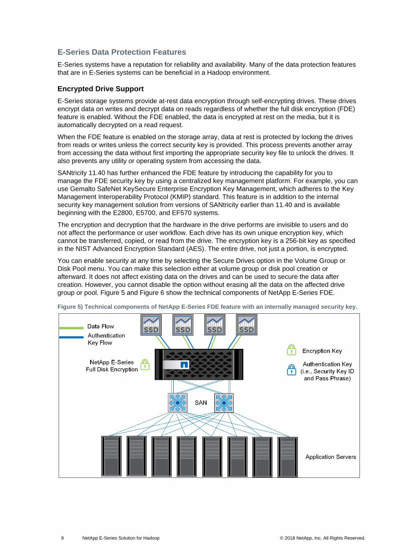
You can enable security at any time by selecting the Secure Drives option in the Volume Group or
Disk Pool menu. You can make this selection either at volume group or disk pool creation or
afterward. It does not affect existing data on the drives and can be used to secure the data after
creation. However, you cannot disable the option without erasing all the data on the affected drive
group or pool. Figure 5 and Figure 6 show the technical components of NetApp E-Series FDE.
Figure 5) Technical components of NetApp E-Series FDE feature with an internally managed security key.
10 NetApp E-Series Solution for Hadoop © 2018 NetApp, Inc. All Rights Reserved.
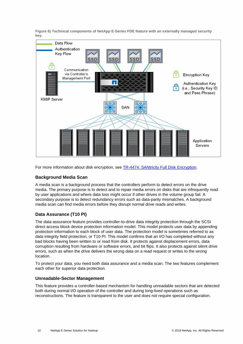
Figure 6) Technical components of NetApp E-Series FDE feature with an externally managed security key.
For more information about disk encryption, see TR-4474: SANtricity Full Disk Encryption.
Background Media Scan
A media scan is a background process that the controllers perform to detect errors on the drive
media. The primary purpose is to detect and to repair media errors on disks that are infrequently read
by user applications and where data loss might occur if other drives in the volume group fail. A
secondary purpose is to detect redundancy errors such as data-parity mismatches. A background
media scan can find media errors before they disrupt normal drive reads and writes.
Data Assurance (T10 PI)
The data assurance feature provides controller-to-drive data integrity protection through the SCSI
direct access block device protection information model. This model protects user data by appending
protection information to each block of user data. The protection model is sometimes referred to as
data integrity field protection, or T10 PI. This model confirms that an I/O has completed without any
bad blocks having been written to or read from disk. It protects against displacement errors, data
corruption resulting from hardware or software errors, and bit flips. It also protects against silent drive
errors, such as when the drive delivers the wrong data on a read request or writes to the wrong
location.
To protect your data, you need both data assurance and a media scan. The two features complement
each other for superior data protection.
Unreadable-Sector Management
This feature provides a controller-based mechanism for handling unreadable sectors that are detected
both during normal I/O operation of the controller and during long-lived operations such as
reconstructions. The feature is transparent to the user and does not require special configuration.
11 NetApp E-Series Solution for Hadoop © 2018 NetApp, Inc. All Rights Reserved.
Proactive Drive-Health Monitor
Proactive drive-health monitoring examines every completed drive I/O and tracks the rate of error and
exception conditions that are returned by the drives. It also tracks drive performance degradation,
which is often associated with unreported internal drive issues. By using predictive failure analysis
technology, when any error rate or degraded performance threshold is exceeded—indicating that a
drive is showing signs of impending failure—SANtricity software issues a critical alert message and
takes corrective action to protect the data.
Data Evacuator
With data evacuator, nonresponsive drives are automatically power-cycled to see whether the fault
condition can be cleared. If the condition cannot be cleared, the drive is flagged as failed. For
predictive failure events, the evacuator feature removes data from the affected drive; this action
moves the data before the drive actually fails. If the drive fails, rebuild picks up where the evacuator
was disrupted, thus reducing the rebuild time.
Hot Spare Support
The system supports global hot spares that can be automatically used by the controller to reconstruct
the data of the failed drive if enough redundancy information is available. The controller selects the
best match for the hot spare based on several factors, including capacity and speed.
SSD Wear-Life Monitoring and Reporting
If an SSD supports wear-life reporting, the GUI gives you this information so that you can monitor how
much of the useful life of an SSD remains. For SSDs that support wear-life monitoring, the percentage
of spare blocks that remain in solid-state media is monitored by controller firmware at approximately
1-hour intervals. Think of this approach as a fuel gauge for SSDs.
SSD Read Cache
The SANtricity SSD read cache feature uses SSD storage to hold frequently accessed data from user
volumes. It is intended to improve the performance of workloads that are performance limited by HDD
IOPS. Workloads with the following characteristics can benefit from using the SANtricity SSD read
cache feature:
• Read performance is limited by HDD IOPS.
• There is a higher percentage of read operations relative to write operations. More than 80% of the operations constitute read.
• Numerous reads are repeat reads to the same or to adjacent areas of the disk.
• The size of the data that is repeatedly accessed is smaller than the SSD read cache capacity.
For more information about SSD read cache, see TR-4099: NetApp SANtricity SSD Cache for
E-Series.
2.3 Performance and Capacity
Performance
An E5700 system that is configured with all SSD, all HDD, or a mixture of both drives can provide high
IOPS and throughput with low latency. Through its ease of management, high degree of reliability,
and exceptional performance, you can use E-Series storage to meet the extreme performance
requirements of a Hadoop cluster deployment.
An E5700 with 24 SSDs can provide up to 1 million 4K random read IOPS at less than 100µs average
response time. This configuration can also deliver 21GBps of read throughput and 9GBps of write
throughput.
Many factors can affect the performance of the E5700, including different volume group types, the use
of DDP technology, the average I/O size, and the read versus write percentage the attached servers
12 NetApp E-Series Solution for Hadoop © 2018 NetApp, Inc. All Rights Reserved.
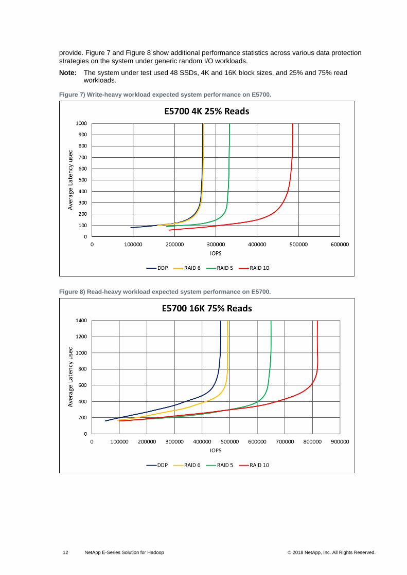
provide. Figure 7 and Figure 8 show additional performance statistics across various data protection
strategies on the system under generic random I/O workloads.
Note: The system under test used 48 SSDs, 4K and 16K block sizes, and 25% and 75% read workloads.
Figure 7) Write-heavy workload expected system performance on E5700.
Figure 8) Read-heavy workload expected system performance on E5700.

13 NetApp E-Series Solution for Hadoop © 2018 NetApp, Inc. All Rights Reserved.
Capacity
The E5760 has a maximum capacity of 4800TB (with expansion drive shelves), using 480 NL-SAS
HDD drives of 10TB each. The E5724 has a maximum capacity of 1800TB (with expansion drive
shelves), using 120 SSD drives of 15.3TB each. See Table 3 for available drive capacities.
Table 3) Available drive capacities for E5700.
Controller Shelf Model
Drive Shelf Model
Number of Drives
NL-SAS HDDs SAS HDDs SSDs
E5760 DE460C
(4U60)
60 4TB
8TB
10TB
900GB
1.2TB
1.8TB
800GB
1.6TB
3.2TB
E5724 DE224C
(2U24)
24 N/A 900GB
1.2TB
1.8TB
800GB
1.6TB
3.2TB
15.3TB
3 Hadoop Enterprise Solution with NetApp
3.1 Data Locality and Its Insignificance for Hadoop
One of the initial primary concepts in Hadoop to improve performance was to move compute to data
or to colocate compute and storage. This approach meant moving the actual compute code to servers
on which the data resides, and not the other way around. Because data is usually larger in size than
the compute code, it might be a challenge to send big data across a network, especially with lower-
bandwidth networks.
However, segregation of storage and compute is necessary to scale up and to maintain flexibility. In
2011, it was estimated that reading data from local disks is only 8% faster than reading it from remote
disks [8], and this number is only decreasing with time. Networks are getting faster, but the disks are
not. As an example, Ananthanarayanan et al. [8] analyzed logs from Facebook and concluded that
“disk-locality results in little, if any, improvement of task lengths.”
With all the advancements being made in improving the network infrastructure, data compression, and
deduplication, it is no longer necessary to colocate storage and compute. In fact, it is better to
segregate storage and compute and to build a flexible and easy-to-scale solution. This area is where
NetApp solutions can help.
3.2 NetApp E-Series
NetApp E-Series systems offer a block-storage solution that is designed for speed. E-Series is a
better fit for applications that need dedicated storage, such as SAN-based business apps; dedicated
backup targets; and high-density storage repositories. The E-Series solution delivers performance
efficiency with an excellent price/performance ratio, from entry- to enterprise-level systems. It also
provides maximum disk I/O for a low cost and delivers sustained high bandwidth and IOPS. E-Series
systems run a separate operating environment, called NetApp SANtricity. All E-Series models support
both SSD and HDD and can be configured with dual controllers for high availability. You can find more
details on the E-Series webpages.
3.3 Hadoop Replication Factor and Total Cost of Ownership
To be fault tolerant and reliable, HDFS allows users to set a replication factor for data blocks. A
replication factor of 3 means that three copies of the data would be stored on HDFS instead of one.
Therefore, even if two drives that store the same data fail, the data is not lost. The trade-off here is an
increase (3 times or more) in space and network utilization. With a traditional JBOD configuration,
setting a replication factor of 3 is recommended to significantly decrease the probability of data loss.
14 NetApp E-Series Solution for Hadoop © 2018 NetApp, Inc. All Rights Reserved.
With DDP technology on a NetApp E-Series storage system, the data and parity information are
distributed across a pool of drives. The DDP intelligent algorithm defines which drives are used for
segment placement, helping to fully protect the data. For more information, see the DDP datasheet.
Because of these intelligent features, NetApp recommends using a replication factor of 2 instead of 3
when using an E-Series storage system. The lower replication factor puts less load on the network,
and jobs complete faster. Therefore, fewer DataNodes are required, which directly relates to spending
less on the licensing fees if you use managed Hadoop software.
Also, because NetApp provides a decoupled Hadoop solution in which compute and storage are
segregated, you no longer need to buy more compute servers for storage-intensive jobs.
3.4 Enterprise-Class Data Protection
Drive failures are common in data centers. Although Hadoop is built to be fault tolerant, a drive failure
can significantly affect performance. Even when using RAID, the drive rebuild times can be several
hours to days, depending on the size of the disk. DDP technology enables consistent and optimal
performance during a drive failure and can rebuild a failed drive up to 8 times faster than RAID can.
This superior performance results from the way that the DDP feature spreads the parity information
and the spare capacity throughout the pool.
3.5 Enterprise-Level Scalability and Flexibility
By using E-Series storage solutions for HDFS, you can separate the two main components of
Hadoop: compute and storage. This decoupled solution provides the flexibility of managing both
components separately. For example, the SANtricity software that comes with the E-Series products
provides an intuitive and user-friendly interface from which extra storage can be added seamlessly.
This flexibility makes it convenient to scale the storage capacity up or down as needed without
affecting any running jobs.
3.6 Hortonworks and Cloudera Certified
NetApp has partnered with Hortonworks and Cloudera to certify the NetApp Hadoop solutions. For
more information, see the Hortonworks and Cloudera websites.
3.7 Easy to Deploy and to Use
There is a steep learning curve for customers who are new to Hadoop. Few enterprise applications
are built to run on massively parallel clusters. However, the NetApp E-Series solution for Hadoop
provides an operational model for a Hadoop cluster that does not require additional attention after its
initial setup. The cluster is more stable and easier to maintain, allowing you to concentrate on meeting
your business needs. This solution flattens the operational learning curve of Hadoop.
4 Experimental Design and Setup
4.1 Architectural Pipeline and Hardware Details
Our test setup uses Hortonworks Hadoop v2.7.3.2.6.2.0-205. We used Apache Ambari [3] for the
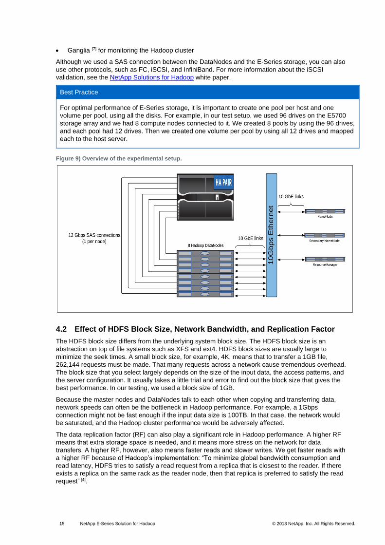
configuration and installation of all components. Figure 9 depicts the architecture, which includes:
• Eight Fujitsu servers (48 vCPUs, 256GB memory) with twelve 4TB drives on each, acting as worker nodes
• Two master servers (24 vCPUs, 64GB memory) serving as the NameNode and resource manager
• All servers using a 10Gb dual-port network connection
• 12Gbps SAS connections to the E-Series storage array
• NetApp E5700 storage solution used for testing
• Ninety-six 6TB HDD (7200 RPM); 8 DDP pools, each having 12 drives, and each pool having 1 volume mapped to 1 host
15 NetApp E-Series Solution for Hadoop © 2018 NetApp, Inc. All Rights Reserved.
• Ganglia [7] for monitoring the Hadoop cluster
Although we used a SAS connection between the DataNodes and the E-Series storage, you can also
use other protocols, such as FC, iSCSI, and InfiniBand. For more information about the iSCSI
validation, see the NetApp Solutions for Hadoop white paper.
Best Practice
For optimal performance of E-Series storage, it is important to create one pool per host and one
volume per pool, using all the disks. For example, in our test setup, we used 96 drives on the E5700
storage array and we had 8 compute nodes connected to it. We created 8 pools by using the 96 drives,
and each pool had 12 drives. Then we created one volume per pool by using all 12 drives and mapped
each to the host server.
Figure 9) Overview of the experimental setup.
4.2 Effect of HDFS Block Size, Network Bandwidth, and Replication Factor
The HDFS block size differs from the underlying system block size. The HDFS block size is an
abstraction on top of file systems such as XFS and ext4. HDFS block sizes are usually large to
minimize the seek times. A small block size, for example, 4K, means that to transfer a 1GB file,
262,144 requests must be made. That many requests across a network cause tremendous overhead.
The block size that you select largely depends on the size of the input data, the access patterns, and
the server configuration. It usually takes a little trial and error to find out the block size that gives the
best performance. In our testing, we used a block size of 1GB.
Because the master nodes and DataNodes talk to each other when copying and transferring data,
network speeds can often be the bottleneck in Hadoop performance. For example, a 1Gbps
connection might not be fast enough if the input data size is 100TB. In that case, the network would
be saturated, and the Hadoop cluster performance would be adversely affected.
The data replication factor (RF) can also play a significant role in Hadoop performance. A higher RF
means that extra storage space is needed, and it means more stress on the network for data
transfers. A higher RF, however, also means faster reads and slower writes. We get faster reads with
a higher RF because of Hadoop’s implementation: “To minimize global bandwidth consumption and
read latency, HDFS tries to satisfy a read request from a replica that is closest to the reader. If there
exists a replica on the same rack as the reader node, then that replica is preferred to satisfy the read
request” [4].
16 NetApp E-Series Solution for Hadoop © 2018 NetApp, Inc. All Rights Reserved.
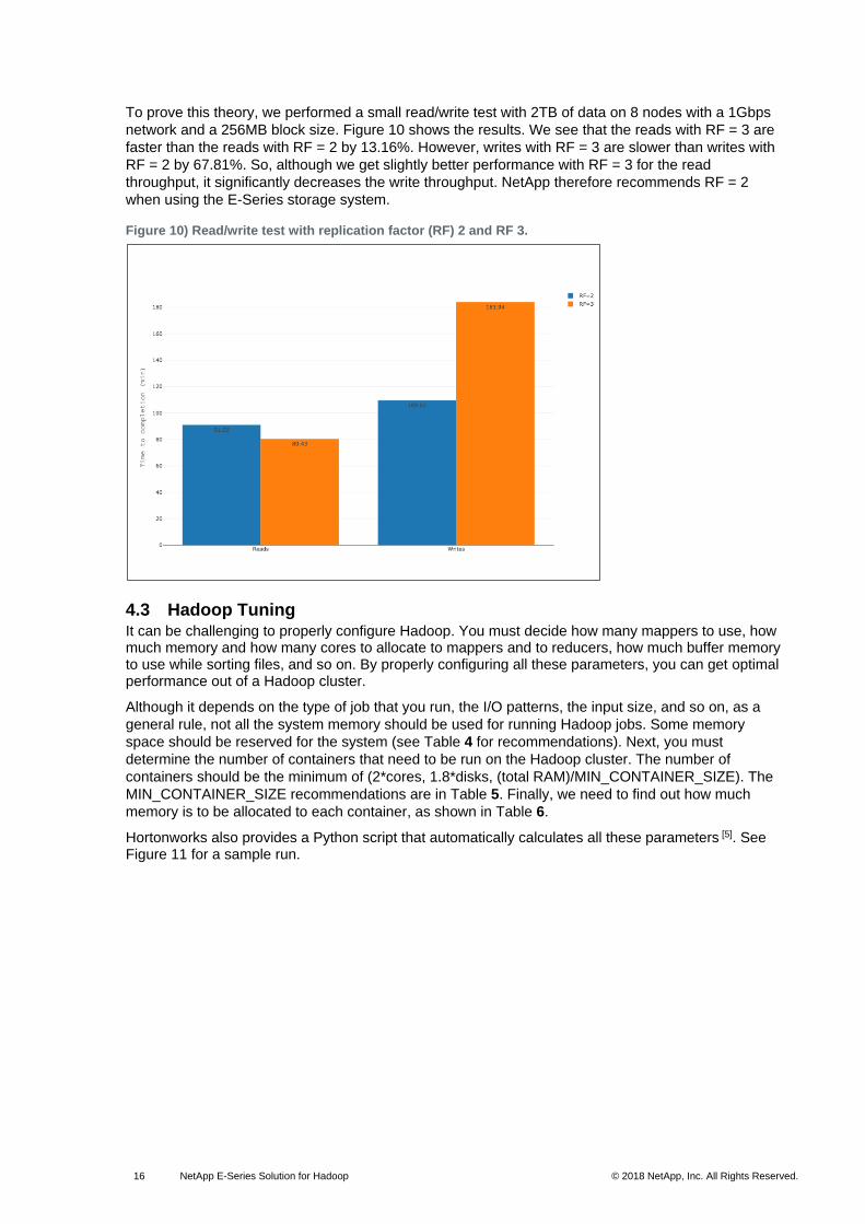
To prove this theory, we performed a small read/write test with 2TB of data on 8 nodes with a 1Gbps
network and a 256MB block size. Figure 10 shows the results. We see that the reads with RF = 3 are
faster than the reads with RF = 2 by 13.16%. However, writes with RF = 3 are slower than writes with
RF = 2 by 67.81%. So, although we get slightly better performance with RF = 3 for the read
throughput, it significantly decreases the write throughput. NetApp therefore recommends RF = 2
when using the E-Series storage system.
Figure 10) Read/write test with replication factor (RF) 2 and RF 3.
4.3 Hadoop Tuning It can be challenging to properly configure Hadoop. You must decide how many mappers to use, how much memory and how many cores to allocate to mappers and to reducers, how much buffer memory to use while sorting files, and so on. By properly configuring all these parameters, you can get optimal performance out of a Hadoop cluster.
Although it depends on the type of job that you run, the I/O patterns, the input size, and so on, as a
general rule, not all the system memory should be used for running Hadoop jobs. Some memory
space should be reserved for the system (see Table 4 for recommendations). Next, you must
determine the number of containers that need to be run on the Hadoop cluster. The number of
containers should be the minimum of (2*cores, 1.8*disks, (total RAM)/MIN_CONTAINER_SIZE). The
MIN_CONTAINER_SIZE recommendations are in Table 5. Finally, we need to find out how much
memory is to be allocated to each container, as shown in Table 6.
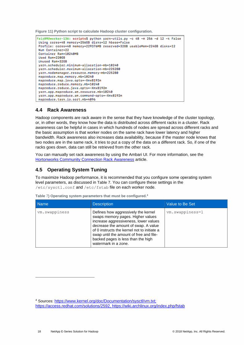
Hortonworks also provides a Python script that automatically calculates all these parameters [5]. See Figure 11 for a sample run.
17 NetApp E-Series Solution for Hadoop © 2018 NetApp, Inc. All Rights Reserved.
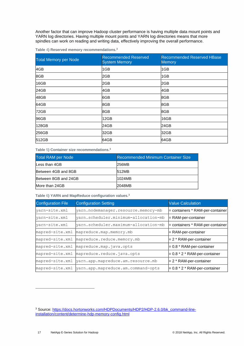
Another factor that can improve Hadoop cluster performance is having multiple data mount points and YARN log directories. Having multiple mount points and YARN log directories means that more spindles can work on reading and writing data, effectively improving the overall performance.
Table 4) Reserved memory recommendations.3
Total Memory per Node Recommended Reserved System Memory
Recommended Reserved HBase Memory
4GB 1GB 1GB
8GB 2GB 1GB
16GB 2GB 2GB
24GB 4GB 4GB
48GB 6GB 8GB
64GB 8GB 8GB
72GB 8GB 8GB
96GB 12GB 16GB
128GB 24GB 24GB
256GB 32GB 32GB
512GB 64GB 64GB
Table 5) Container size recommendations.3
Total RAM per Node Recommended Minimum Container Size
Less than 4GB 256MB
Between 4GB and 8GB 512MB
Between 8GB and 24GB 1024MB
More than 24GB 2048MB
Table 6) YARN and MapReduce configuration values.3
Configuration File Configuration Setting Value Calculation
yarn-site.xml yarn.nodemanager.resource.memory-mb = containers * RAM-per-container
yarn-site.xml yarn.scheduler.minimum-allocation-mb = RAM-per-container
yarn-site.xml yarn.scheduler.maximum-allocation-mb = containers * RAM-per-container
mapred-site.xml mapreduce.map.memory.mb = RAM-per-container
mapred-site.xml mapreduce.reduce.memory.mb = 2 * RAM-per-container
mapred-site.xml mapreduce.map.java.opts = 0.8 * RAM-per-container
mapred-site.xml mapreduce.reduce.java.opts = 0.8 * 2 * RAM-per-container
mapred-site.xml yarn.app.mapreduce.am.resource.mb = 2 * RAM-per-container
mapred-site.xml yarn.app.mapreduce.am.command-opts = 0.8 * 2 * RAM-per-container
3 Source: https://docs.hortonworks.com/HDPDocuments/HDP2/HDP-2.6.0/bk_command-line-installation/content/determine-hdp-memory-config.html
18 NetApp E-Series Solution for Hadoop © 2018 NetApp, Inc. All Rights Reserved.
Figure 11) Python script to calculate Hadoop cluster configuration.
4.4 Rack Awareness
Hadoop components are rack aware in the sense that they have knowledge of the cluster topology,
or, in other words, they know how the data is distributed across different racks in a cluster. Rack
awareness can be helpful in cases in which hundreds of nodes are spread across different racks and
the basic assumption is that worker nodes on the same rack have lower latency and higher
bandwidth. Rack awareness also increases data availability, because if the master node knows that
two nodes are in the same rack, it tries to put a copy of the data on a different rack. So, if one of the
racks goes down, data can still be retrieved from the other rack.
You can manually set rack awareness by using the Ambari UI. For more information, see the
Hortonworks Community Connection Rack Awareness article.
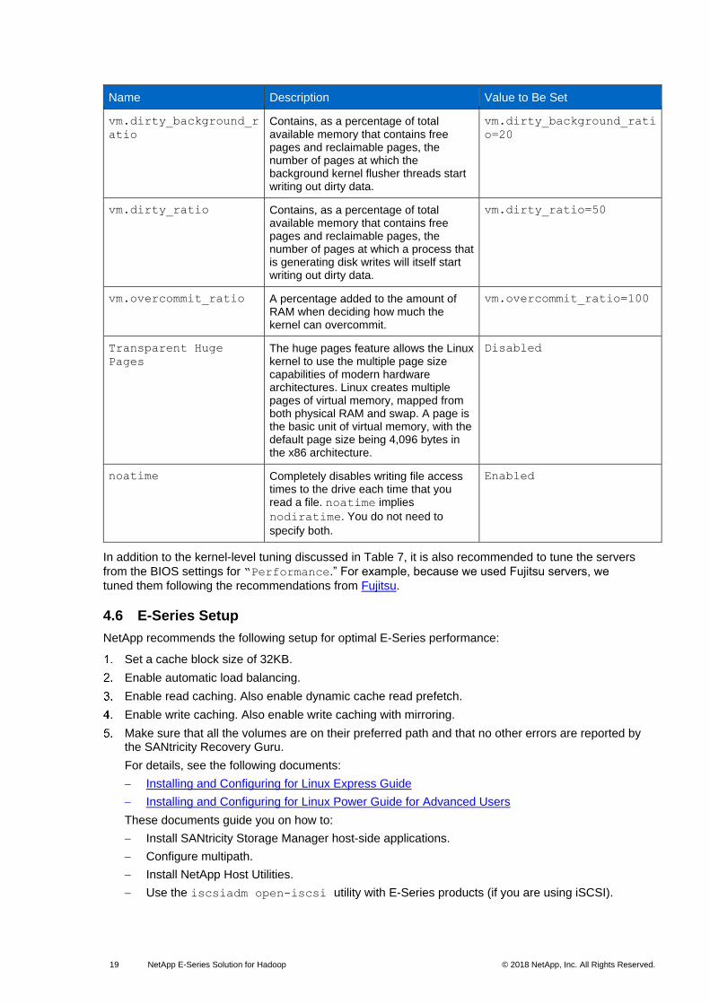
4.5 Operating System Tuning
To maximize Hadoop performance, it is recommended that you configure some operating system
level parameters, as discussed in Table 7. You can configure these settings in the
/etc/sysctl.conf and /etc/fstab file on each worker node.
Table 7) Operating system parameters that must be configured.4
Name Description Value to Be Set
vm.swappiness Defines how aggressively the kernel swaps memory pages. Higher values increase aggressiveness, lower values decrease the amount of swap. A value of 0 instructs the kernel not to initiate a swap until the amount of free and file-backed pages is less than the high watermark in a zone.
vm.swappiness=1
4 Sources: https://www.kernel.org/doc/Documentation/sysctl/vm.txt;
https://access.redhat.com/solutions/2592, https://wiki.archlinux.org/index.php/fstab
19 NetApp E-Series Solution for Hadoop © 2018 NetApp, Inc. All Rights Reserved.
Name Description Value to Be Set
vm.dirty_background_r
atio
Contains, as a percentage of total available memory that contains free pages and reclaimable pages, the number of pages at which the background kernel flusher threads start writing out dirty data.
vm.dirty_background_rati
o=20
vm.dirty_ratio Contains, as a percentage of total available memory that contains free pages and reclaimable pages, the number of pages at which a process that is generating disk writes will itself start writing out dirty data.
vm.dirty_ratio=50
vm.overcommit_ratio A percentage added to the amount of RAM when deciding how much the kernel can overcommit.
vm.overcommit_ratio=100
Transparent Huge
Pages
The huge pages feature allows the Linux kernel to use the multiple page size capabilities of modern hardware architectures. Linux creates multiple pages of virtual memory, mapped from both physical RAM and swap. A page is the basic unit of virtual memory, with the default page size being 4,096 bytes in the x86 architecture.
Disabled
noatime Completely disables writing file access times to the drive each time that you read a file. noatime implies
nodiratime. You do not need to
specify both.
Enabled
In addition to the kernel-level tuning discussed in Table 7, it is also recommended to tune the servers
from the BIOS settings for “Performance.” For example, because we used Fujitsu servers, we
tuned them following the recommendations from Fujitsu.
4.6 E-Series Setup
NetApp recommends the following setup for optimal E-Series performance:
Set a cache block size of 32KB.
Enable automatic load balancing.
Enable read caching. Also enable dynamic cache read prefetch.
Enable write caching. Also enable write caching with mirroring.
Make sure that all the volumes are on their preferred path and that no other errors are reported by the SANtricity Recovery Guru.
For details, see the following documents:
Installing and Configuring for Linux Express Guide
Installing and Configuring for Linux Power Guide for Advanced Users
These documents guide you on how to:
Install SANtricity Storage Manager host-side applications.
Configure multipath.
Install NetApp Host Utilities.
Use the iscsiadm open-iscsi utility with E-Series products (if you are using iSCSI).
20 NetApp E-Series Solution for Hadoop © 2018 NetApp, Inc. All Rights Reserved.
To verify that your configuration is supported and to check for any changes that might be required for
the correct functioning of your E-Series system, see the Interoperability Matrix Tool.
4.7 NetApp In-Place Analytics Module
In addition to Hadoop solutions that are based on E-Series, the NetApp FAS controller provides in-
place Hadoop analytics through the NetApp In-Place Analytics Module for Hadoop. This module is
based on the Apache standard open implementation. For details, see TR-4382: NetApp FAS NFS
Connector for Hadoop.
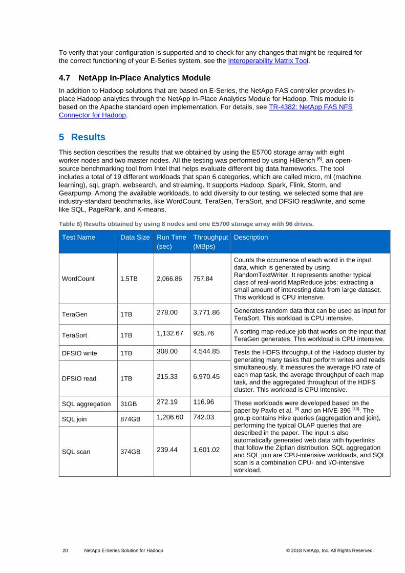
5 Results
This section describes the results that we obtained by using the E5700 storage array with eight
worker nodes and two master nodes. All the testing was performed by using HiBench [6], an open-
source benchmarking tool from Intel that helps evaluate different big data frameworks. The tool
includes a total of 19 different workloads that span 6 categories, which are called micro, ml (machine
learning), sql, graph, websearch, and streaming. It supports Hadoop, Spark, Flink, Storm, and
Gearpump. Among the available workloads, to add diversity to our testing, we selected some that are
industry-standard benchmarks, like WordCount, TeraGen, TeraSort, and DFSIO read/write, and some
like SQL, PageRank, and K-means.
Table 8) Results obtained by using 8 nodes and one E5700 storage array with 96 drives.
Test Name Data Size Run Time
(sec)
Throughput
(MBps)
Description
WordCount 1.5TB 2,066.86 757.84
Counts the occurrence of each word in the input data, which is generated by using RandomTextWriter. It represents another typical class of real-world MapReduce jobs: extracting a small amount of interesting data from large dataset. This workload is CPU intensive.
TeraGen 1TB 278.00 3,771.86 Generates random data that can be used as input for TeraSort. This workload is CPU intensive.
TeraSort 1TB 1,132.67 925.76 A sorting map-reduce job that works on the input that TeraGen generates. This workload is CPU intensive.
DFSIO write 1TB 308.00 4,544.85 Tests the HDFS throughput of the Hadoop cluster by generating many tasks that perform writes and reads simultaneously. It measures the average I/O rate of each map task, the average throughput of each map task, and the aggregated throughput of the HDFS cluster. This workload is CPU intensive.
DFSIO read 1TB 215.33 6,970.45
SQL aggregation 31GB 272.19 116.96 These workloads were developed based on the paper by Pavlo et al. [9] and on HIVE-396 [10]. The group contains Hive queries (aggregation and join), performing the typical OLAP queries that are described in the paper. The input is also automatically generated web data with hyperlinks that follow the Zipfian distribution. SQL aggregation and SQL join are CPU-intensive workloads, and SQL scan is a combination CPU- and I/O-intensive workload.
SQL join 874GB 1,206.60 742.03
SQL scan 374GB 239.44 1,601.02

21 NetApp E-Series Solution for Hadoop © 2018 NetApp, Inc. All Rights Reserved.
Test Name Data Size Run Time
(sec)
Throughput
(MBps)
Description
PageRank 32GB 1,241.85 26.02
Benchmarks the PageRank algorithm implemented in Spark-MLlib/Hadoop (a search engine ranking benchmark that is included in Pegasus 2.0) examples. The data source is generated from web data whose hyperlinks follow the Zipfian distribution. It is a mixture of a CPU- and I/O-intensive workload.
K-means 224GB 1,844.80 124.58
Tests the K-means (a well-known clustering algorithm for knowledge discovery and data mining) clustering in Spark MLlib. GenKMeansDataset generates the input dataset based on Uniform Distribution and Gaussian Distribution. This workload is CPU intensive.
Table 8 shows the time to completion for all the tests and shows the throughput achieved. In most cases, the throughput for the tests is simply calculated by the ratio of the data size and the time to completion. The exceptions are the DFSIO read and DFSIO write tests, in which the throughput calculations are based on the throughput reported by TestDFSIO times the minimum of (nrFiles, VCores total – 1). For details, see the blog post about Benchmarking and Stress Testing an Hadoop Cluster With TeraSort, TestDFSIO & Co. Therefore, the I/O-intensive DFSIO read and DFSIO write tests provide a better representation of the overall throughput capabilities of the E5700 storage array than do the other CPU-intensive tests.
The tests that are shown in Table 8 produced slightly different results each time that they were run. Hence, each test was run multiple times, and the average was noted. Running each test requires a little bit of trial and error to determine the combination that works best. For example, a 1GB HDFS block size can give better performance than a 128MB block size depending on how fast the worker nodes are completing the maps. As a general rule, the Hadoop cluster should be configured in a manner such that each mapper task takes at least more than 1 minute to finish.
The E5700 storage array is optimal for building a robust, flexible, scalable, and high-throughput Hadoop cluster that is expected to run production-level jobs. Although we used only 96 HDDs in our testing, the E5700 array can support up to 480 drives; the maximum number of drives will achieve better throughput. The advantages of using the NetApp E-Series solution, as discussed in section 3, make the E5700 a leader in building Hadoop solutions.
6 Hadoop Sizing
To estimate the appropriate size of a Hadoop cluster, you must know the following:
• Estimated storage requirements
• Estimated compute power needed, or the overall Hadoop cluster throughput needed
With this information, you can estimate how many HDFS building blocks you need to meet the
requirements. Each building block can consist of 4 or 8 worker nodes and one E-Series storage array
with 60 or 120 drives. You might need to consider aspects such as the data replication factor (NetApp
recommends a replication factor of 2 when using the E-Series system). You should also make sure
that HDFS does not use all the storage space, that it leaves behind some space for the system and
for Hadoop logs, and so on.
To help you determine the approximate number of building blocks that you need, consider the
following example:
A customer has 1PB of data and expects that amount to increase by 30% over the next three years.
The customer plans to use DDP technology, and the cluster must ingest 10TB of data each night. All
10TB must be loaded in an hour or less. The customer's data analytics job uses all the new data for
the night and must be completed within 30 minutes or less. The estimated I/O mix for analytics jobs is
100% read and 0% write:
22 NetApp E-Series Solution for Hadoop © 2018 NetApp, Inc. All Rights Reserved.
• Over a period of 3 years, the data would become 1PB + 30% of 1PB, which is equal to 1.3PB. Assuming a replication factor of 2, the data size would become 2.6PB. Let’s keep 1TB of space for the system and for Hadoop logs, and so on. Therefore, the total storage needed is 2.7PB.
• Assuming that 1 building block uses approximately 120 disks of 6TB, the maximum storage capacity that each building block can have is around 660TB (assuming that only 5.5TB is usable of a 6TB drive). Therefore, to store 2.7PB of data, we need 4.2 building blocks.
• The ingest rate is 10TB every night. Assuming that the customer wants to use the E5700, it would take almost 39 minutes for 1 building block to ingest the data. To calculate ingest time, the write speed as shown in Table 8 for E5700 is 4.438GBps. Therefore, (10*1,024)/(4.438*60) gives us the time in minutes to ingest the data), which is below the customer’s requirement of one hour.
• The read speed of E5700 as shown in Table 8 is 6.807GBps. Therefore, to process 10TB data, it would take almost 25 minutes for 1 building block to finish, which is below the customer’s requirement of 30 minutes.
7 Conclusion
This document discusses best practices for creating a Hadoop cluster and how the NetApp E-Series
storage system can help your organization attain maximum throughout when running Hadoop jobs.
With the NetApp Hadoop solution, you can decrease the overall cost of ownership and gain enhanced
data security, flexibility, and easy scalability. These benefits were demonstrated in our testing, in
which the NetApp E5700 (higher-end) storage system was benchmarked by running 10 different
Hadoop workloads.
8 Future Work
The tests described in this report were run on the E5700 (higher-end) storage array. In the future, the
same tests will be run on the E2800 (lower-end) storage array to evaluate the difference in
performance. This testing will help our customers ascertain which storage array best meets their
requirements based on their throughput needs.
Acknowledgments
I would like to thank the following NetApp experts for their input and their assistance:
• Karthikeyan Nagalingam, Senior Architect (Big Data Analytics and Databases)
• Mitch Blackburn, Technical Marketing Engineer
• Esther Smitha, Technical Writer
• Anna Giaconia, Copy Editor
• Lee Dorrier, Director, Data Fabric Group
• Steven Graham, Network Systems AdministratorDanny Landes, Technical Marketing Engineer
• Hoseb Dermanilian, Business Development Manager EMEA, Big Data Analytics and Video Surveillance
• Nilesh Bagad, Senior Product Manager
References
ScienceDaily. “Big Data, for better or worse: 90% of world's data generated over last two years.” May 22, 2013. https://www.sciencedaily.com/releases/2013/05/130522085217.htm (accessed December 22, 2017).
Ghemawat, S., Gobioff, H., and Leung, S.-T., “The Google File System,” ACM SIGOPS Operating Systems Review, vol. 37, no. 5., December 2003.
Apache Software Foundation. “Getting Started with Ambari.” https://ambari.apache.org/ (accessed December 22, 2017).
23 NetApp E-Series Solution for Hadoop © 2018 NetApp, Inc. All Rights Reserved.
Hadoop. “HDFS Architecture Guide.” Last published August 4, 2013. https://hadoop.apache.org/docs/r1.2.1/hdfs_design.html (accessed December 22, 2017).
Hortonworks. “Command Line Installation.” 2017. https://docs.hortonworks.com/HDPDocuments/HDP2/HDP-2.6.0/bk_command-line-installation/content/download-companion-files.html (accessed December 22, 2017).
Intel. “intel-hadoop / HiBench.” 2017. https://github.com/intel-hadoop/HiBench (accessed December 22, 2017).
SourceForge. “What is Ganglia?” 2016. http://ganglia.sourceforge.net (accessed December 22, 2017).
Ananthanarayanan, G., Ghodsi, A., Shenker, S., and Stoica, I., “Disk-Locality in Datacenter Computing Considered Irrelevant.” In HotOS ’13, Proceedings of the 13th USENIX Conference on Hot Topics in Operating Systems, vol. 13, May 2011, pp. 12–12.
Pavlo, A., Paulson, E., Rasin, A., Abadi, D. J., DeWitt, D. J., Madden, S., & Stonebraker, M., “A Comparison of Approaches to Large-Scale Data Analysis.” In Proceedings of the 2009 ACM SIGMOD International Conference on Management of data, June 2009, pp. 165-178.
Apache. “Hive performance benchmarks”. 2016. https://issues.apache.org/jira/browse/HIVE-396 (accessed March 1, 2018).
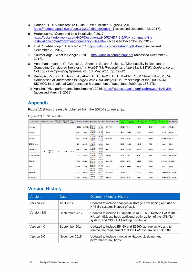
Appendix
Figure 12 shows the results obtained from the E5700 storage array.
Figure 12) E5700 results.
Version History
Version Date Document Version History
Version 2.0 April 2012 Updated to include changes in storage provisioning and use of XFS file systems instead of ext3.
Version 3.0 September 2012 Updated to include OS update to RHEL 6.2, NetApp FAS2040 HA pair, diskless boot, additional optimization of the XFS file system, and CDH3U4 Hadoop distribution.
Version 4.0 September 2014 Updated to include E5460 and E5560 storage arrays and to remove the requirement that the FAS system be a FAS2040.
Version 5.0 November 2015 Updated to include innovative Hadoop 2, sizing, and performance solutions.

24 NetApp E-Series Solution for Hadoop © 2018 NetApp, Inc. All Rights Reserved.
Version Date Document Version History
Version 6.0 March 2018 Removed redundant content, benchmarked E5700, added new tests, removed old system tuning parameters.

25 NetApp E-Series Solution for Hadoop © 2018 NetApp, Inc. All Rights Reserved.
Refer to the Interoperability Matrix Tool (IMT) on the NetApp Support site to validate that the exact product and feature versions described in this document are supported for your specific environment. The NetApp IMT defines the product components and versions that can be used to construct configurations that are supported by NetApp. Specific results depend on each customer’s installation in accordance with published specifications.
Copyright Information
Copyright © 1994–2018 NetApp, Inc. All Rights Reserved. Printed in the U.S. No part of this document covered by copyright may be reproduced in any form or by any means—graphic, electronic, or mechanical, including photocopying, recording, taping, or storage in an electronic retrieval system—without prior written permission of the copyright owner.
Software derived from copyrighted NetApp material is subject to the following license and disclaimer:
THIS SOFTWARE IS PROVIDED BY NETAPP “AS IS” AND WITHOUT ANY EXPRESS OR IMPLIED WARRANTIES, INCLUDING, BUT NOT LIMITED TO, THE IMPLIED WARRANTIES OF MERCHANTABILITY AND FITNESS FOR A PARTICULAR PURPOSE, WHICH ARE HEREBY DISCLAIMED. IN NO EVENT SHALL NETAPP BE LIABLE FOR ANY DIRECT, INDIRECT, INCIDENTAL, SPECIAL, EXEMPLARY, OR CONSEQUENTIAL DAMAGES (INCLUDING, BUT NOT LIMITED TO, PROCUREMENT OF SUBSTITUTE GOODS OR SERVICES; LOSS OF USE, DATA, OR PROFITS; OR BUSINESS INTERRUPTION) HOWEVER CAUSED AND ON ANY THEORY OF LIABILITY, WHETHER IN CONTRACT, STRICT LIABILITY, OR TORT (INCLUDING NEGLIGENCE OR OTHERWISE) ARISING IN ANY WAY OUT OF THE USE OF THIS SOFTWARE, EVEN IF ADVISED OF THE POSSIBILITY OF SUCH DAMAGE.
NetApp reserves the right to change any products described herein at any time, and without notice. NetApp assumes no responsibility or liability arising from the use of products described herein, except as expressly agreed to in writing by NetApp. The use or purchase of this product does not convey a license under any patent rights, trademark rights, or any other intellectual property rights of NetApp.
The product described in this manual may be protected by one or more U.S. patents, foreign patents, or pending applications.
RESTRICTED RIGHTS LEGEND: Use, duplication, or disclosure by the government is subject to restrictions as set forth in subparagraph (c)(1)(ii) of the Rights in Technical Data and Computer Software clause at DFARS 252.277-7103 (October 1988) and FAR 52-227-19 (June 1987).
Trademark Information
NETAPP, the NETAPP logo, and the marks listed at http://www.netapp.com/TM are trademarks of NetApp, Inc. Other company and product names may be trademarks of their respective owners.
TR-3969-0318
Related Documents