TR 101 613 - V1.1.1 - Intelligent Transport Systems (ITS ... · Cross Layer DCC Management Entity for operation in the ITS G5A and ... "Intelligent Transport Systems (ITS); Cross

ETSI TR 101 613 V1.1.1 (2015-09)

Intelligent Transport Systems (ITS); Cross Layer DCC Management Entity

for operation in the ITS G5A and ITS G5B medium; Validation set-up and results

TECHNICAL REPORT

ETSI

ETSI TR 101 613 V1.1.1 (2015-09) 2

Reference DTR/ITS-0020056

Keywords ITS, Spectral Management

ETSI

650 Route des Lucioles F-06921 Sophia Antipolis Cedex - FRANCE

Tel.: +33 4 92 94 42 00 Fax: +33 4 93 65 47 16

Siret N° 348 623 562 00017 - NAF 742 C

Association à but non lucratif enregistrée à la Sous-Préfecture de Grasse (06) N° 7803/88

Important notice

The present document can be downloaded from: http://www.etsi.org/standards-search

The present document may be made available in electronic versions and/or in print. The content of any electronic and/or print versions of the present document shall not be modified without the prior written authorization of ETSI. In case of any

existing or perceived difference in contents between such versions and/or in print, the only prevailing document is the print of the Portable Document Format (PDF) version kept on a specific network drive within ETSI Secretariat.

Users of the present document should be aware that the document may be subject to revision or change of status. Information on the current status of this and other ETSI documents is available at

http://portal.etsi.org/tb/status/status.asp

If you find errors in the present document, please send your comment to one of the following services: https://portal.etsi.org/People/CommiteeSupportStaff.aspx

Copyright Notification

No part may be reproduced or utilized in any form or by any means, electronic or mechanical, including photocopying and microfilm except as authorized by written permission of ETSI.

The content of the PDF version shall not be modified without the written authorization of ETSI. The copyright and the foregoing restriction extend to reproduction in all media.

© European Telecommunications Standards Institute 2015.

All rights reserved.

DECTTM, PLUGTESTSTM, UMTSTM and the ETSI logo are Trade Marks of ETSI registered for the benefit of its Members. 3GPPTM and LTE™ are Trade Marks of ETSI registered for the benefit of its Members and

of the 3GPP Organizational Partners. GSM® and the GSM logo are Trade Marks registered and owned by the GSM Association.

http://www.etsi.org/standards-search

http://portal.etsi.org/tb/status/status.asp

https://portal.etsi.org/People/CommiteeSupportStaff.aspx

ETSI

ETSI TR 101 613 V1.1.1 (2015-09) 3

Contents Intellectual Property Rights ................................................................................................................................ 5

Foreword ............................................................................................................................................................. 5

Modal verbs terminology .................................................................................................................................... 5

Executive summary ............................................................................................................................................ 5

1 Scope ........................................................................................................................................................ 6

2 References ................................................................................................................................................ 6

2.1 Normative references ......................................................................................................................................... 6

2.2 Informative references ........................................................................................................................................ 6

3 Definitions, symbols and abbreviations ................................................................................................... 8

3.1 Definitions .......................................................................................................................................................... 8

3.2 Symbols .............................................................................................................................................................. 8

3.3 Abbreviations ..................................................................................................................................................... 8

4 DCC theory .............................................................................................................................................. 9

5 Simulation results ................................................................................................................................... 10

5.1 Characteristics of common algorithms ............................................................................................................. 10

5.1.1 Reactive table based algorithm ................................................................................................................... 10

5.1.1.1 Simulator 1: Conclusions ...................................................................................................................... 10

5.1.1.2 Simulator 1: Introduction ...................................................................................................................... 10

5.1.1.3 Simulator 1: Tools and setup ................................................................................................................. 11

5.1.1.4 Simulation 1.1: Study on the synchronization issue of the DCC .......................................................... 14

5.1.1.5 Simulation 1.2: Study on channel load characterization ....................................................................... 20

5.1.1.6 Simulation 1.3: Study on non-identical sensing capabilities ................................................................. 22

5.1.2 Adaptive linear control algorithms ............................................................................................................. 23

5.1.3 Comparison of different common algorithms ............................................................................................. 23


5.1.3.2 Simulator 2: Tools and Setup ................................................................................................................ 24

5.1.3.3 Simulator 2: Simulation results ............................................................................................................. 26

5.2 Mixed use of different algorithms .................................................................................................................... 28

5.2.1 Simulator 3: Conclusions ............................................................................................................................ 28

5.2.2 Simulator 3: Introduction ............................................................................................................................ 28

5.2.2.1 Overview ............................................................................................................................................... 28

5.2.2.2 DCC background ................................................................................................................................... 29

5.2.2.3 CAM-DCC algorithm............................................................................................................................ 29

5.2.2.4 LIMERIC algorithm .............................................................................................................................. 30

5.2.3 Simulator 3: Tools and setup ...................................................................................................................... 30

5.2.3.1 Simulation tools .................................................................................................................................... 30

5.2.3.2 Simulator configuration ........................................................................................................................ 30

5.2.3.3 CAM-DCC implementation .................................................................................................................. 31

5.2.3.4 LIMERIC implementation .................................................................................................................... 32

5.2.3.5 Simulation scenarios ............................................................................................................................. 32

5.2.3.6 Alternate CAM-DCC lookup table parameters ..................................................................................... 33

5.2.3.7 Alternate LIMERIC target CBP ............................................................................................................ 33

5.2.3.8 Simulations with the different parameter settings for the algorithms .................................................... 33

5.2.4 Simulator 3: Simulation results ................................................................................................................... 33

5.2.4.1 Introduction to the results ...................................................................................................................... 33

5.2.4.2 Simulation 3.1: Default parameter setting ............................................................................................. 34

5.2.4.3 Discussion on the performance difference of CAM-DCC and LIMERIC in the mixed network ......... 36

5.2.4.4 Simulation 3.2: Modified lookup table.................................................................................................. 36

5.2.4.5 Simulation 3.3: Modified LIMERIC target value ................................................................................. 37

5.2.4.6 Simulation 3.4: Modified look-up table and LIMERIC target value ..................................................... 39

5.3 Future aspects and algorithms .......................................................................................................................... 40

5.3.1 ECPR algorithm .......................................................................................................................................... 40

5.3.1.1 Simulator 4: Conclusions ...................................................................................................................... 40


ETSI

ETSI TR 101 613 V1.1.1 (2015-09) 4

5.3.1.3 Simulator 4: Tools and setup ................................................................................................................. 41

5.3.1.4 ECPR Algorithm: Testing Different Target Rate and Awareness Distance Sets for - Urban vs. Highway Environment .......................................................................................................................... 44

5.3.1.5 Comparing ECPR, LIMERIC, Power-only, and No-DCC algorithm ................................................... 45

History .............................................................................................................................................................. 50

ETSI

ETSI TR 101 613 V1.1.1 (2015-09) 5

Intellectual Property Rights IPRs essential or potentially essential to the present document may have been declared to ETSI. The information pertaining to these essential IPRs, if any, is publicly available for ETSI members and non-members, and can be found in ETSI SR 000 314: "Intellectual Property Rights (IPRs); Essential, or potentially Essential, IPRs notified to ETSI in respect of ETSI standards", which is available from the ETSI Secretariat. Latest updates are available on the ETSI Web server (http://ipr.etsi.org).

Pursuant to the ETSI IPR Policy, no investigation, including IPR searches, has been carried out by ETSI. No guarantee can be given as to the existence of other IPRs not referenced in ETSI SR 000 314 (or the updates on the ETSI Web server) which are, or may be, or may become, essential to the present document.

Foreword This Technical Report (TR) has been produced by ETSI Technical Committee Intelligent Transport Systems (ITS).

Modal verbs terminology In the present document "shall", "shall not", "should", "should not", "may", "need not", "will", "will not", "can" and "cannot" are to be interpreted as described in clause 3.2 of the ETSI Drafting Rules (Verbal forms for the expression of provisions).

"must" and "must not" are NOT allowed in ETSI deliverables except when used in direct citation.

Executive summary The documented simulations prove that there are functional methods to manage channel load.

Different metrics have been selected to compare the effectiveness and fairness of different methods, and also possible coexistence of adaptive and reactive algorithms has been demonstrated in simulations.

Despite currently defined methods and individual parameters, in future even more complex methods and algorithms for managing channel load can be expected to evolve.

http://webapp.etsi.org/IPR/home.asp

http://portal.etsi.org/Help/editHelp!/Howtostart/ETSIDraftingRules.aspx

ETSI

ETSI TR 101 613 V1.1.1 (2015-09) 6

1 Scope The present document covers the overall validation of the cross layer DCC functionality of the ETSI ITS architecture. It considers the cross layer DCC specification developed in ETSI TS 103 175 [i.1] and the cross layer concept described in ETSI TR 101 612 [i.2] and all other relevant DCC components in the communication stack.

2 References

2.1 Normative references References are either specific (identified by date of publication and/or edition number or version number) or non-specific. For specific references, only the cited version applies. For non-specific references, the latest version of the reference document (including any amendments) applies.

Referenced documents which are not found to be publicly available in the expected location might be found at http://docbox.etsi.org/Reference.

NOTE: While any hyperlinks included in this clause were valid at the time of publication, ETSI cannot guarantee their long term validity.

The following referenced documents are necessary for the application of the present document.

Not applicable.

2.2 Informative references References are either specific (identified by date of publication and/or edition number or version number) or non-specific. For specific references, only the cited version applies. For non-specific references, the latest version of the reference document (including any amendments) applies.

NOTE: While any hyperlinks included in this clause were valid at the time of publication, ETSI cannot guarantee their long term validity.

The following referenced documents are not necessary for the application of the present document but they assist the user with regard to a particular subject area.

[i.1] ETSI TS 103 175: "Intelligent Transport Systems (ITS); Cross Layer DCC Management Entity for operation in the ITS G5A and ITS G5B medium".

[i.2] ETSI TR 101 612: "Intelligent Transport Systems (ITS); Cross Layer DCC Management Entity for operation in the ITS G5A and ITS G5B medium; Report on Cross layer DCC algorithms and performance evaluation".

[i.3] IEEE 802.11-2012: "IEEE Standard for Information technology -- Telecommunications and information exchange between systems Local and metropolitan area networks -- Specific requirements Part 11: Wireless LAN Medium Access Control (MAC) and Physical Layer (PHY) Specifications".

[i.4] ETSI EN 302 663: "Intelligent Transport Systems (ITS); Access layer specification for Intelligent Transport Systems operating in the 5 GHz frequency band".

[i.5] ETSI TS 102 687 (V1.1.1): "Intelligent Transport Systems (ITS); Decentralized Congestion Control Mechanisms for Intelligent Transport Systems operating in the 5 GHz range; Access layer part".

[i.6] ETSI EN 302 637-2: "Intelligent Transport Systems (ITS); Vehicular Communications; Basic Set of Applications; Part 2: Specification of Cooperative Awareness Basic Service".

[i.7] Oyunchimeg Shagdar: "Evaluation of Synchronous and Asynchronous Reactive Distributed Congestion Control Algorithms for the ITS G5 Vehicular Systems", Technical Report 462, INRIA Paris-Rocquencourt. 2015. <hal-01168043>.

http://docbox.etsi.org/Reference

ETSI

ETSI TR 101 613 V1.1.1 (2015-09) 7

[i.8] ns-2, network simulator, http://www.isi.edu/nsnam/ns/, https://en.wikipedia.org/wiki/Ns-(simulator).

[i.9] ns-3, network simulator, http://www.nsnam.org, https://en.wikipedia.org/wiki/Ns_(simulator).

[i.10] SUMO, Simulation of Urban mobility, http://www.dlr.de/ts/en/desktopdefault.aspx/, http://sumo-sim.org/.

[i.11] Osama Al-Gazali, Jérôme Härri: "Performance Evaluation of Reactive and Adaptive DCC Algorithms for Safety-Related Vehicular Communications", Master Thesis, EURECOM, January 2015.

[i.12] M. Behrisch, L. Bieker, J. Erdmann, and D. Kajzewicz: "Sumo-simulation of urban mobility-an overview", SIMUL 2011, The Third International Conference on Advances in System Simulation. 2011.

[i.13] D. Krajzewicz: "Sumo (simulation of urban mobility)", Proc. of the 4th middle east symposium on simulation and modelling, 2002.

[i.14] ns-3 WAVE module, http://www.nsnam.org/docs/models/html/wave.html.

[i.15] R. Jain, D. Chiu, and W. Hawe: "A Quantitative Measure Of Fairness And Discrimination For Resource Allocation In Shared Computer Systems", DEC, Research Report TR-301, September 1984.

[i.16] Kenney. J.B, Bansal. G, Rohrs. C.E, LIMERIC: "A linear message rate control algorithm for vehicular DSRC systems", 8th ACM Int. Workshop on Vehicular Inter-networking VANET 11, pp. 21-30, 2011.

[i.17] G. Bansal, J. Kenney, C. Rohrs: "LIMERIC: A Linear Adaptive Message Rate Algorithm for DSRC Congestion Control", IEEE Transactions on Vehicular Technology, Vol. 62, No. 9, pp. 4182-4197, Nov. 2013.

[i.18] G. Bansal, H. Lu, J. Kenney, and C. Poellabauer: "EMBARC: Error model based adaptive rate control for vehicle-to-vehicle communications", Proc. 10th ACM Int. Workshop on Vehicular Inter-Networking, Systems, Applications (VANET 2013), June 2013, pp. 41-50.

[i.19] G. Bansal, B. Cheng, A. Rostami, K. Sjoberg, J. Kenney, and M. Gruteser: "Comparing LIMERIC and DCC approaches for VANET channel congestion control", Wireless Vehicular Communications (WiVeC), 2014 IEEE 6th International Symposium on, pp. 1-7, 2014.

[i.20] B. Aygun, M. Boban, A. Wyglinski: "ECPR: Environment-aware Combined Power and Rate Distributed Congestion Control for Vehicular Communication", arXiv preprint arXiv:1502.00054: http://arxiv-web3.library.cornell.edu/abs/1502.00054.

[i.21] M. Boban, J. Barros, and O. K. Tonguz: "Geometry-Based Vehicle-to-Vehicle Channel Modeling for Large-Scale Simulation", IEEE Transactions on Vehicular Technology, Vol. 63, No. 9, pp. 4146-4164, Nov. 2014.

[i.22] Open Street Map, topological data base, http://www.openstreetmap.org/.

[i.23] M. Boban and P. d'Orey: "Measurement-based evaluation of cooperative awareness for V2V and V2I communication", IEEE Vehicular Networking Conference (VNC 2014), December 2014, pp. 1-8.

[i.24] Claudia Campolo, Antonella Molinaro, Riccardo Scopigno: "Vehicular ad hoc Networks, Standards, Solutions, and Research", ISBN: 978-3-319-15496-1 (Print), 978-3-319-15497-8 (Online).

[i.25] "Highway Capacity Manual", Transportation Research Board, Washington, D.C. 2010. ISBN 978-0-309-16077-3.

http://www.isi.edu/nsnam/ns/

https://en.wikipedia.org/wiki/Ns-(simulator)

https://en.wikipedia.org/wiki/Ns-(simulator)

http://www.nsnam.org/

https://en.wikipedia.org/wiki/Ns_(simulator)

http://www.dlr.de/ts/en/desktopdefault.aspx/

http://sumo-sim.org/

http://sumo-sim.org/

http://www.nsnam.org/docs/models/html/wave.html

http://arxiv-web3.library.cornell.edu/abs/1502.00054

http://www.openstreetmap.org/

ETSI

ETSI TR 101 613 V1.1.1 (2015-09) 8

3 Definitions, symbols and abbreviations

3.1 Definitions For the purposes of the present document, the terms and definitions given in ETSI TS 103 175 [i.1], ETSI TR 101 612 [i.2] and the following apply:

NAV: busy flag defined in [i.3]

ns-3: discrete-event network simulator for Internet systems, targeted primarily for research and educational use.

NOTE: ns-3 is free software, licensed under the GNU GPLv2 license, and is publicly available for research, development, and use.

3.2 Symbols For the purposes of the present document, the following symbols apply:

α Adaption parameter that control the DCC algorithm β Adaption parameter that control the DCC algorithm δ Default packet length for the simulations CBPTarget Target channel load

CBRn CBR measured at the nth monitoring interval

CLn Channel load calculated upon measurement of CBRn

N_GenCam Maximum number of consecutive CAM generations due to the elapsed time since the last CAM generation

NDL_maxChannelLoad The channel is considered to be overloaded if the CBP is larger than this value NDL_minChannelLoad The channel is considered to be mainly free if the CBP is smaller than this value NDL_TimeDown controls how fast DCC reacts to channel load decrease NDL_TimeUp controls how fast DCC reacts to channel load increase rj Message rate of ITS-S j

TBUSY, Tbusy Total time during which the channel is indicated as busy during Tmon

T_GenCam Currently valid upper limit of the CAM generation interval T_CheckCamGen Time period for checking the generation of a new safety message T_GenCam_Dcc Initial CAM generation time interval. T_GenCamMin No CAM can be generated with an interval smaller than this variable T_GenCamMax No CAM can be generated with an interval greater than this variable Tmonitor, Tmon CBR monitoring interval

3.3 Abbreviations For the purposes of the present document, the following abbreviations apply:

A-DCC Adaptive DCC AIFS Arbitration Inter Frame Space BSM Basic Safety Message BTP Basic Transport Protocol CAM Cooperative Awareness Message CBP Channel Busy Percentage CBR Channel Busy Ratio CCA Clear Channel Assessment CCH Control Channel CL Channel Load DCC Decentralized Congestion Control DENM Decentralized Environmental Notification Message ECPR Environment- and Context-aware Combined Power and Rate distributed congestion control EDCA Enhanced Distributed Channel Access FIR Finite Impulse Response

ETSI

ETSI TR 101 613 V1.1.1 (2015-09) 9

GPS Global Positioning System iCS iTetris Control System IP Internet Protocol IPG Inter-Packet Gap ITS Intelligent Transportation System ITS-G5 Radio interface, collectively known as the 5 GHz ITS frequency band ITS-S ITS Station LIMERIC LInear MEssage Rate Integrated Control LOS Line Of Sight LOS-C stable flow Level-of-Service of traffic conditions

NOTE: As defined in [i.25].

LOS-F fully saturated (breakdown flow) Level-of-Service of traffic conditions

NOTE: As defined in [i.25].

MAC Medium Access Control NAR Neighborhood Awareness Ratio PDR Packet Delivery Ratio PER Packet Error Rate PHY Physical Layer PIR Packet Inter-Reception time QPSK Quadrature Phase-Shift Keying R-DCC Reactive DCC RNAR Ratio of Neighbors Above Range SINR Signal to Interference and Noise Ratio SUMO Simulation of Urban MObility TA Target Awareness TC Traffic Class TCP/IP Transmission Control Protocol/Internet Protocol T-DCC DCC with solely CAM triggering conditions TX Transmit UDP User Datagram Protocol UDP/IP User Datagram Protocol/Internet Protocol UK United Kingdom US United States WAVE Wireless Access in Vehicular Environments WLAN Wireless Local Area Network

4 DCC theory The aim of DCC is to avoid overloading the ITS-G5 radio channel. This can be done by different means as specified in ETSI TS 102 687 [i.5].

It has been shown recently that a pure message rate control can effectively limit the channel load [i.24], therefore most of the simulation results presented in the present document focus on this type of DCC. Clause 5.3 gives an outlook of how DCC can be even further improved to not only avoid channel overload, but also maximise the awareness about other vehicles in the vicinity.

When designing a message rate DCC algorithm the following key fundamentals are important:

• Convergence to a single message rate by all network nodes

• Bounded stability in the sense that message rate changes over time should be within small bounds

Further details about convergence and stability are summarised in [i.24].

ETSI

ETSI TR 101 613 V1.1.1 (2015-09) 10

5 Simulation results

5.1 Characteristics of common algorithms

5.1.1 Reactive table based algorithm

5.1.1.1 Simulator 1: Conclusions

Using Simulator 1, the following issues targeting reactive dynamic DCC algorithm are studied.

• DCC synchronization

• Channel load characterization

• Non-identical receiver parameters

The following conclusions are drawn:

• It is very important to provide a solution to avoid the synchronization of DCC behaviour among ITS-S. If a careful attention is given on this issue, the simple reactive DCC algorithm can perform better than having no DCC (hereunder called DccOff). In the case of rate adaptation, introducing a random message generation rate offset seems to be a good solution, but is not further investigated in the present document.

• If the road traffic is sparse, the reactive DCC algorithm tends to show poorer performance than DccOff.

• Resetting the message generation timer based on the actual CBR value is not advantageous.

• If the ITS-S transmits unsynchronized, the current CBR is a good indicator of the channel load. However, if the transmissions are synchronized, it is necessary to pay attention on CBR for a longer interval.

• If the system consists of ITS-S with heterogeneous channel sensing capability, non-negligible negative impact can be expected in terms of communications range and fairness.

• The fairness issue caused by non-identical sensing capabilities is more significant for DCC-enabled system.

5.1.1.2 Simulator 1: Introduction

The results of simulator 1 are detailed in paper [i.7], using a simulation tool combining ns-3 (network simulator) and SUMO (Simulation of urban mobility). Simulator 1 implemented the reactive DCC algorithm, controlling the message rate following a parameter look-up table (shown in table 2).

Following simulations are performed with simulator 1:

• Simulation 1.1: Study on the synchronization issue of the DCC.

• Simulation 1.2: Study on channel load characterization.

• Simulation 1.3: Study on non-identical sensing capabilities.

Simulation 1.1 investigates the handling of the channel busy ratio (CBR), which is the ratio of the time when the channel is perceived as busy to the monitoring interval. It is the commonly agreed metric used to characterize channel load. Since the wireless channel is shared by ITS-S that are in the vicinity of each other, the CBR monitored at such ITS-S takes similar values. As a consequence, the ITS-S may take synchronized reactions to the channel load, e.g. the ITS-S reduce/increase the transmission rate at around the same time. Simulation 1.1 studies such a synchronized DCC behaviour observed in reactive DCC algorithm. The following different possible reactions of the CAM generator, which is responsible for adjusting the message generation rate as a means to perform DCC, were studied:

• Timer handling: In general, a transmission of a CAM is triggered by a timer, which is set to the CAM interval. Hence, upon being informed with a new CBR value (at an arbitrary point of time), the CAM generator may:

1) wait the expiration of the on-going timer and set the timer to the new CAM interval; or

ETSI

ETSI TR 101 613 V1.1.1 (2015-09) 11

2) cancel the on-going timer and set it to the new CAM interval. The former and latter behaviours are respectively named Wait-and-Go and Cancel-and-Go.

• Interval setting: As mentioned above, the CBR measured for the shared channel may lead to the situation where the nearby ITS-S increase/decrease the CAM interval at around the same time. This is especially true for the reactive DCC algorithm, which controls the rate following a parameter look-up table. Therefore, one can think of avoiding such a synchronized behaviour by applying random intervals. Hence, two possible behaviours can be envisioned: upon determination of a new CBR value, in the simulation the CAM generator sets the message generation interval to:

1) the value (say new_CAM_interval) provided by the table; or

2) a random value (e.g. taken from the range [0, new_CAM_interval]) for the first packet and then follows the table.

The former and latter behaviours are respectively named Synchronized and Unsynchronized. In practice, synchronization could happen when the CAM transmissions are triggered based on the common GPS clock.

Considering the above-mentioned behaviours of the CAM generator, the following four different versions of Reactive DCC are simulated:

• DccReactive-1: Wait-and-Go & Synchronized

• DccReactive-2: Cancel-and-Go & Synchronized

• DccReactive-3: Wait-and-Go & Unsynchronized

• DccReactive-4: Cancel-and-Go & Unsynchronized

Simulation 1.1 studies and compares the performances of these different versions of reactive DCC to understand the synchronization issue and their underlying reasons.

Simulation 1.2 investigates the optimum time interval for the channel load characterization. While it is commonly agreed that CBR should be monitored over a certain interval (e.g. 100 ms), it is not clear whether the channel load should be characterized only by the current value of CBR or whether it should also consider the past CBR values. To evaluate this aspect, channel load (CL) is defined as follows.

CLn = (1 - α) × CLn-1 + α × CBRn (1)

In equation 1, CBRn is the CBR measured at the nth monitoring interval and CLn is the channel load calculated upon

measurement of CBRn. The weight factor α defines whether the channel load considers only the last CBR or also takes its

history into account by applying a discrete time first order low pass filtering to the CBR. Obviously, by choosing α = 1, the channel load is characterized by the "current" channel condition only. In simulation 1.2 the performances of a reactive DCC algorithm for different values of α is evaluated.

Simulation 1.3 studies the DCC performance in heterogeneous road systems, made of ITS-S with different levels of sensing capability. Specifically, it is considered that different ITS-S sense the wireless channel at different threshold levels; as a consequence CL is measured differently, what leads to different reactions of each ITS-S. To perform this study, the ITS-S in the simulations are provided with random sensitivity offset values in the range of [-6, +6] dBm.

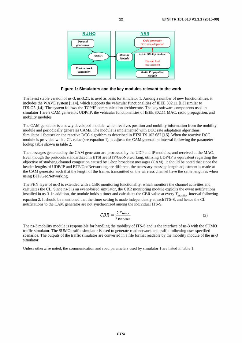
5.1.1.3 Simulator 1: Tools and setup

Simulator 1 uses the open discrete event simulation environment ns-3 (version 3.21) [i.9], combined with the traffic simulator SUMO (version 0.22) [i.10]. The key simulation modules, which are relevant to simulator 1, are illustrated in figure 1, where the modules highlighted in red are newly developed extensions to ns-3.

ETSI

ETSI TR 101 613 V1.1.1 (2015-09) 12

Figure 1: Simulators and the key modules relevant to the work

The latest stable version of ns-3, ns-3.21, is used as basis for simulator 1. Among a number of new functionalities, it includes the WAVE system [i.14], which supports the vehicular functionalities of IEEE 802.11 [i.3] similar to ITS-G5 [i.4]. The system follows the TCP/IP communication architecture. The key software components used in simulator 1 are a CAM generator, UDP/IP, the vehicular functionalities of IEEE 802.11 MAC, radio propagation, and mobility modules.

The CAM generator is a newly developed module, which receives position and mobility information from the mobility module and periodically generates CAMs. The module is implemented with DCC rate adaptation algorithms. Simulator 1 focuses on the reactive DCC algorithm as described in ETSI TS 102 687 [i.5]. When the reactive DCC module is provided with a CL value (see equation 1), it adjusts the CAM generation interval following the parameter lookup table shown in table 2.

The messages generated by the CAM generator are processed by the UDP and IP modules, and received at the MAC. Even though the protocols standardized in ETSI are BTP/GeoNetworking, utilizing UDP/IP is equivalent regarding the objective of studying channel congestion caused by 1-hop broadcast messages (CAM). It should be noted that since the header lengths of UDP/IP and BTP/GeoNetworking are different, the necessary message length adjustment is made at the CAM generator such that the length of the frames transmitted on the wireless channel have the same length as when using BTP/GeoNetworking.

The PHY layer of ns-3 is extended with a CBR monitoring functionality, which monitors the channel activities and calculates the CL. Since ns-3 is an event-based simulator, the CBR monitoring module exploits the event notifications installed in ns-3. In addition, the module holds a timer and calculates the CBR value at every Tmonitor interval following

equation 2. It should be mentioned that the timer setting is made independently at each ITS-S, and hence the CL notifications to the CAM generator are not synchronized among the individual ITS-S.

�� =

∑��

�� (2)

The ns-3 mobility module is responsible for handling the mobility of ITS-S and is the interface of ns-3 with the SUMO traffic simulator. The SUMO traffic simulator is used to generate road network and traffic following user-specified scenarios. The outputs of the traffic simulator are converted in a file format readable by the mobility module of the ns-3 simulator.

Unless otherwise noted, the communication and road parameters used by simulator 1 are listed in table 1.

NS3SUMO

Demand generation

Road network generation

SUMO Mobility Module

CAM generatorDCC rate adaptation

IEEE 802.11p module

Channel load measurement

Radio Propagation module

ETSI

ETSI TR 101 613 V1.1.1 (2015-09) 13

Table 1: Default simulation parameters of simulator 1

Parameters Value Communication

CAM default TX rate 10 Hz CAM message size 400 Bytes

TX Power 23 dBm EDthreshold -95 dBm

EDCA Queue/TC 1 DENM/3 CAM Modulation scheme QPSK ½ 6 Mbits/s

Antenna pattern Omnidirectional, gain = 1 dBi Access technology ITS G5A

ITS G5 Channel CCA Fading model LogDistance, exponent 2

Road network Lane width 3 m

Lanes in-flow 3 Lanes contra-flow 3

DCC parameters CBR monitor interval (Tmonitor) 100 ms

α (see (1)) 1

The parameter table of the reactive DCC algorithm is shown in table 2.

Table 2: Reactive DCC parameter lookup table used in simulator 1

States CL (%) Toff

Relaxed 0 % ≤ CL < 19 % 60 Active_1 19 % ≤ CL < 27 % 100 Active_2 27 % ≤ CL < 35 % 180 Active_3 35 % ≤ CL < 43 % 260 Active_4 43 % ≤ CL < 51 % 340 Active_5 51 % ≤ CL < 59 % 420

Restricted CL ≥ 59 % 460

The simulations are carried out for homogenous highway scenarios. Table 3 provides the road configuration. As shown in table 3 and illustrated in figure 2, the roadside ITS-S are installed every 100 m in the road centre (i.e. the separation between the two centre lanes).

The scenario consists of sparse, medium, dense, and extreme dense traffic. The density parameters are listed in table 4.

Table 3: Simulator 1 road configuration

Class Inter-vehicle distance Highway length 1 000 m

Lanes/Directions 3 lanes/2 directions Roadside ITS-S inter-location 100 m

Vehicle size 2 m x 5 m

Figure 2: Illustration of a homogenous highway scenario used by simulator 1

ETSI

ETSI TR 101 613 V1.1.1 (2015-09) 14

Table 4: Simulator 1 traffic density parameters for homogenous highway scenarios

Class Inter-Vehicle distance Mobility Sparse 100 m inter-distance (3 lanes/2 directions) Static/Mobile Medium 45 m inter-distance (3 lanes/2directions) Static/Mobile Dense 20 m inter-distance (3 lanes/2directions) Static/Mobile

Extreme 100 m inter-distance (3 lanes/2directions) Static

The following metrics are used for performance investigations of simulator 1.

• Packet delivery ratio (PDR): the ratio of the number of received packets to the number of transmitted (generated) packets. PDR is measured at individual ITS-S (vehicles and roadside) targeting CAMs transmitted by each mobile ITS-S (i.e. vehicles).

• Packet Inter-Reception time (PIR): time gap between consecutive CAM messages. PIR is measured at individual ITS-S for received CAMs from each mobile ITS-S.

• Number of transmissions: the total number of CAM transmissions is counted for 20 milliseconds of time bins.

• CBR: the average CBR is calculated for 20 milliseconds of time bins.

• Jain's fairness index [i.15] is calculated for the total number of transmissions from individual mobile ITS-Ss.

5.1.1.4 Simulation 1.1: Study on the synchronization issue of the DCC

In the present clause the results of the four different versions of Reactive DCC are shown for a homogeneous static highway scenario: DccReactive-1, DccReactive-2, DccReactive-3, and DccReactive-4. The performances of these mechanisms are compared with DccOff, which is the ITS-G5 MAC without distributed congestion control.

Figure 3 plots the average PDR of the reactive DCC mechanisms in contrast to that of DccOff. The horizontal axis is the distance between the receivers and the transmitters. DccOff shows an optimum PDR performance in the sparse scenario (defined in table 4), where the channel is not congested. The channel congestion becomes an issue for medium, dense and extreme density classes, where PDR degrades down to 10 % in DccOff. DccReactive mechanisms show better PDR than DccOff. The PDR improvement is much more significant for unsynchronized DCC schemes (DccReactive-3 and DccReactive-4) than for synchronized scheme (DccReactive-1 and DccReactive-2). For timer handling, Cancel-and-Go schemes show poorer performances (DccReactive-2 in comparison to DccReactive-1 and DccReactive-4 in comparison to DccReactive-3).

ETSI

ETSI TR 101 613 V1.1.1 (2015-09) 15

Figure 3: Comparison of Packet Delivery Ratio for different density classes

Figure 4 plots the average PIR of the reactive DCC mechanisms in contrast to that of DccOff. Similar to the PDR case, DccOff shows an excellent PIR performance in the sparse scenario, but the performance largely degrades for higher density classes and it can exceed one second in the extreme density class. The reactive DCC mechanisms show better or worse PIR performances, depending on the synchronized or unsynchronized behaviour. Both synchronized schemes, DccReactive-1 and DccReactive-2, show poorer performance w.r.t . DccOff, except for the case of DccReactive-1 (Wait-and-Go) in the extreme density class. On the other hand, the unsynchronized schemes, DccReactive-3 and DccReactive-4, provide improved performances for dense and extreme classes. The performance improvement is significant for the DccReactive-3 (Wait-and-go & Unsynchronized) and the performance degradation is significant for DccReactive-2 (Cancel-and-Go & Synchronized).

0

0.1

0.2

0.3

0.4

0.5

0.6

0.7

0.8

0.9

1

0 100 200 300 400 500 0

0.1

0.2

0.3

0.4

0.5

0.6

0.7

0.8

0.9

1

Pack

et d

eliv

ery

ratio

Distance (m)

DccOff-SparseDccReactive_1-Sparse

DccOff-MediumDccReactive_1-Medium

DccOff-DenseDccReactive_1-Dense

DccOff-ExtremeDccReactive_1-Extreme

0

0.1

0.2

0.3

0.4

0.5

0.6

0.7

0.8

0.9

1

0 100 200 300 400 500 0

0.1

0.2

0.3

0.4

0.5

0.6

0.7

0.8

0.9

1

Pack

et d

eliv

ery

ratio

Distance (m)





0

0.1

0.2

0.3

0.4

0.5

0.6

0.7

0.8

0.9

1

0 100 200 300 400 500 0

0.1

0.2

0.3

0.4

0.5

0.6

0.7

0.8

0.9

1

Pack

et d

eliv

ery

ratio

Distance (m)





0

0.1

0.2

0.3

0.4

0.5

0.6

0.7

0.8

0.9

1

0 100 200 300 400 500 0

0.1

0.2

0.3

0.4

0.5

0.6

0.7

0.8

0.9

1

Pac

ket d

eliv

ery

ratio

Distance (m)





ETSI

ETSI TR 101 613 V1.1.1 (2015-09) 16

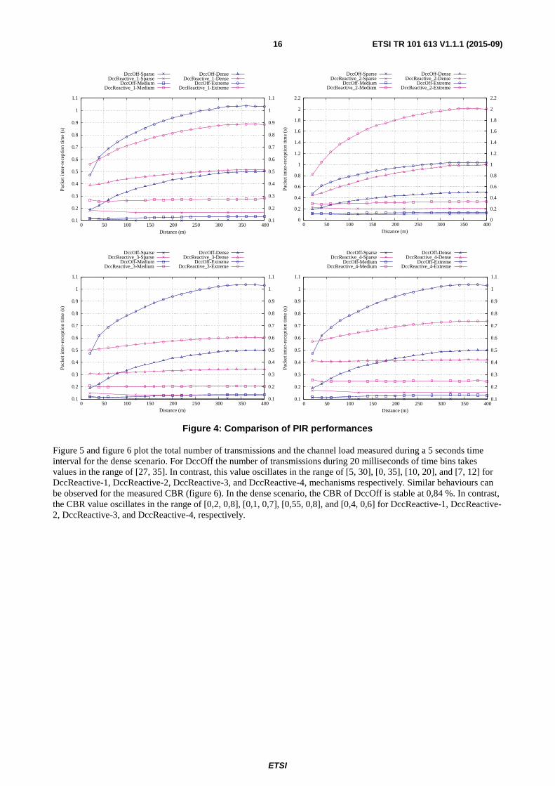
Figure 4: Comparison of PIR performances

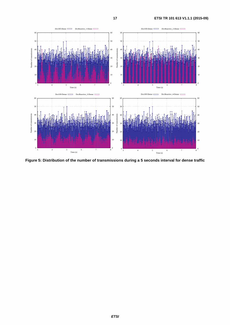
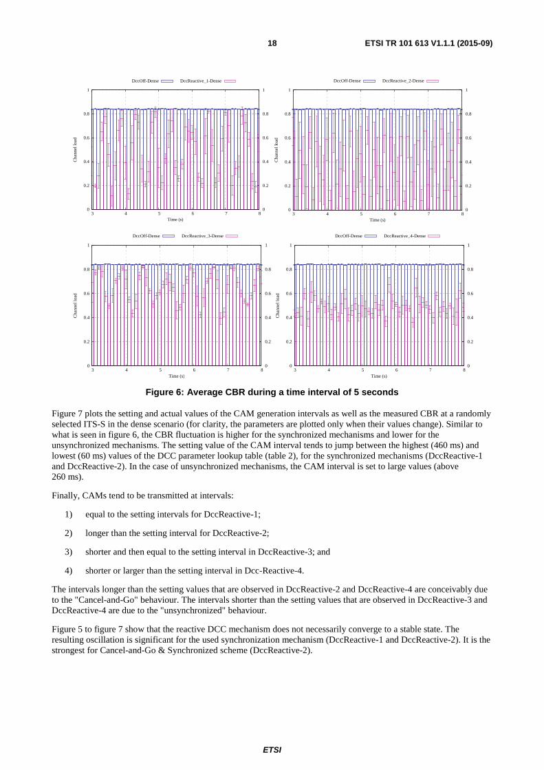
Figure 5 and figure 6 plot the total number of transmissions and the channel load measured during a 5 seconds time interval for the dense scenario. For DccOff the number of transmissions during 20 milliseconds of time bins takes values in the range of [27, 35]. In contrast, this value oscillates in the range of [5, 30], [0, 35], [10, 20], and [7, 12] for DccReactive-1, DccReactive-2, DccReactive-3, and DccReactive-4, mechanisms respectively. Similar behaviours can be observed for the measured CBR (figure 6). In the dense scenario, the CBR of DccOff is stable at 0,84 %. In contrast, the CBR value oscillates in the range of [0,2, 0,8], [0,1, 0,7], [0,55, 0,8], and [0,4, 0,6] for DccReactive-1, DccReactive-2, DccReactive-3, and DccReactive-4, respectively.

0.1

0.2

0.3

0.4

0.5

0.6

0.7

0.8

0.9

1

1.1

0 50 100 150 200 250 300 350 400 0.1

0.2

0.3

0.4

0.5

0.6

0.7

0.8

0.9

1

1.1

Pack

et in

ter-

rece

ptio

n ti

me

(s)

Distance (m)





0

0.2

0.4

0.6

0.8

1

1.2

1.4

1.6

1.8

2

2.2

0 50 100 150 200 250 300 350 400 0

0.2

0.4

0.6

0.8

1

1.2

1.4

1.6

1.8

2

2.2

Pack

et in

ter-

rece

ptio

n tim

e (s

)

Distance (m)





0.1

0.2

0.3

0.4

0.5

0.6

0.7

0.8

0.9

1

1.1

0 50 100 150 200 250 300 350 400 0.1

0.2

0.3

0.4

0.5

0.6

0.7

0.8

0.9

1

1.1

Pack

et in

ter-

rece

ptio

n tim

e (s

)

Distance (m)





0.1

0.2

0.3

0.4

0.5

0.6

0.7

0.8

0.9

1

1.1

0 50 100 150 200 250 300 350 400 0.1

0.2

0.3

0.4

0.5

0.6

0.7

0.8

0.9

1

1.1

Pack

et in

ter-

rece

ptio

n tim

e (s

)

Distance (m)





ETSI

ETSI TR 101 613 V1.1.1 (2015-09) 17

Figure 5: Distribution of the number of transmissions during a 5 seconds interval for dense traffic

0

10

20

30

40

50

60

3 4 5 6 7 8 0

10

20

30

40

50

60N

umbe

r of

tran

smis

sion

s

Time (s)

DccOff-Dense DccReactive_1-Dense

0

10

20

30

40

50

60

3 4 5 6 7 8 0

10

20

30

40

50

60

Num

ber

of tr

ansm

issi

ons

Time (s)


0

10

20

30

40

50

60

3 4 5 6 7 8 0

10

20

30

40

50

60

Num

ber

of tr

ansm

issi

ons

Time (s)


0

10

20

30

40

50

60

3 4 5 6 7 8 0

10

20

30

40

50

60

Num

ber

of tr

ansm

issi

ons

Time (s)


ETSI

ETSI TR 101 613 V1.1.1 (2015-09) 18

Figure 6: Average CBR during a time interval of 5 seconds

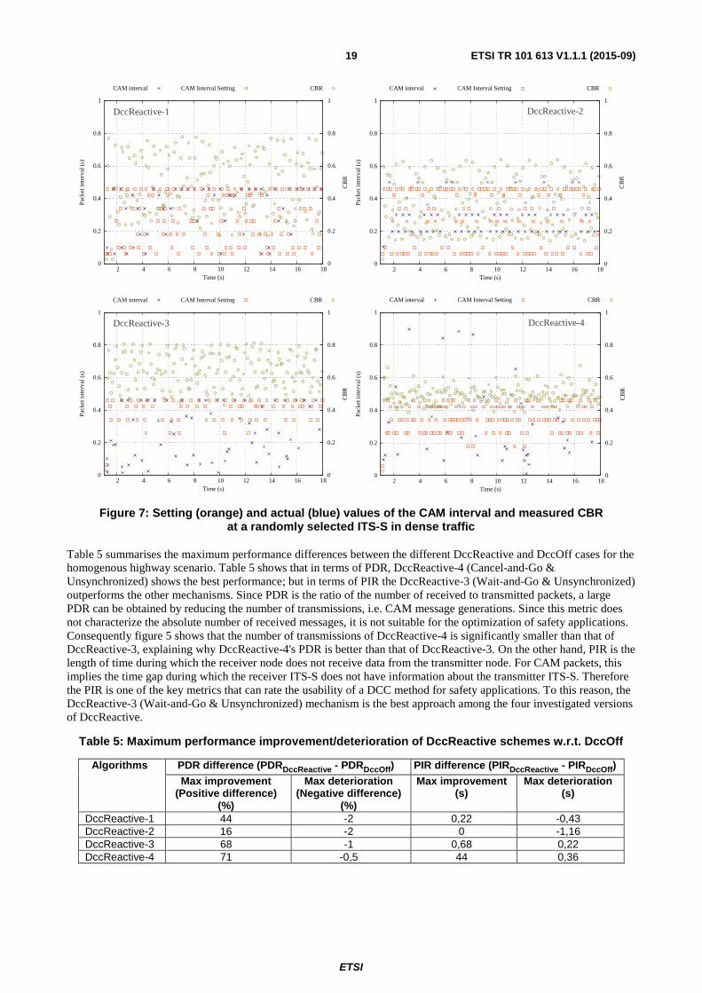
Figure 7 plots the setting and actual values of the CAM generation intervals as well as the measured CBR at a randomly selected ITS-S in the dense scenario (for clarity, the parameters are plotted only when their values change). Similar to what is seen in figure 6, the CBR fluctuation is higher for the synchronized mechanisms and lower for the unsynchronized mechanisms. The setting value of the CAM interval tends to jump between the highest (460 ms) and lowest (60 ms) values of the DCC parameter lookup table (table 2), for the synchronized mechanisms (DccReactive-1 and DccReactive-2). In the case of unsynchronized mechanisms, the CAM interval is set to large values (above 260 ms).

Finally, CAMs tend to be transmitted at intervals:

1) equal to the setting intervals for DccReactive-1;

2) longer than the setting interval for DccReactive-2;

3) shorter and then equal to the setting interval in DccReactive-3; and

4) shorter or larger than the setting interval in Dcc-Reactive-4.

The intervals longer than the setting values that are observed in DccReactive-2 and DccReactive-4 are conceivably due to the "Cancel-and-Go" behaviour. The intervals shorter than the setting values that are observed in DccReactive-3 and DccReactive-4 are due to the "unsynchronized" behaviour.

Figure 5 to figure 7 show that the reactive DCC mechanism does not necessarily converge to a stable state. The resulting oscillation is significant for the used synchronization mechanism (DccReactive-1 and DccReactive-2). It is the strongest for Cancel-and-Go & Synchronized scheme (DccReactive-2).

0

0.2

0.4

0.6

0.8

1

3 4 5 6 7 8 0

0.2

0.4

0.6

0.8

1

Cha

nnel

load

Time (s)


0

0.2

0.4

0.6

0.8

1

3 4 5 6 7 8 0

0.2

0.4

0.6

0.8

1

Cha

nnel

load

Time (s)


0

0.2

0.4

0.6

0.8

1

3 4 5 6 7 8 0

0.2

0.4

0.6

0.8

1

Cha

nnel

load

Time (s)


0

0.2

0.4

0.6

0.8

1

3 4 5 6 7 8 0

0.2

0.4

0.6

0.8

1

Cha

nnel

load

Time (s)


ETSI

ETSI TR 101 613 V1.1.1 (2015-09) 19

Figure 7: Setting (orange) and actual (blue) values of the CAM interval and measured CBR at a randomly selected ITS-S in dense traffic

Table 5 summarises the maximum performance differences between the different DccReactive and DccOff cases for the homogenous highway scenario. Table 5 shows that in terms of PDR, DccReactive-4 (Cancel-and-Go & Unsynchronized) shows the best performance; but in terms of PIR the DccReactive-3 (Wait-and-Go & Unsynchronized) outperforms the other mechanisms. Since PDR is the ratio of the number of received to transmitted packets, a large PDR can be obtained by reducing the number of transmissions, i.e. CAM message generations. Since this metric does not characterize the absolute number of received messages, it is not suitable for the optimization of safety applications. Consequently figure 5 shows that the number of transmissions of DccReactive-4 is significantly smaller than that of DccReactive-3, explaining why DccReactive-4's PDR is better than that of DccReactive-3. On the other hand, PIR is the length of time during which the receiver node does not receive data from the transmitter node. For CAM packets, this implies the time gap during which the receiver ITS-S does not have information about the transmitter ITS-S. Therefore the PIR is one of the key metrics that can rate the usability of a DCC method for safety applications. To this reason, the DccReactive-3 (Wait-and-Go & Unsynchronized) mechanism is the best approach among the four investigated versions of DccReactive.

Table 5: Maximum performance improvement/deterioration of DccReactive schemes w.r.t. DccOff

Algorithms PDR difference (PDRDccReactive - PDRDccOff) PIR difference (PIRDccReactive - PIRDccOff)

Max improvement (Positive difference)

(%)

Max deterioration (Negative difference)

(%)

Max improvement (s)

Max deterioration (s)

DccReactive-1 44 -2 0,22 -0,43 DccReactive-2 16 -2 0 -1,16 DccReactive-3 68 -1 0,68 0,22 DccReactive-4 71 -0,5 44 0,36

0

0.2

0.4

0.6

0.8

1

2 4 6 8 10 12 14 16 18 0

0.2

0.4

0.6

0.8

1

Pac

ket i

nter

val (

s)

CB

R

Time (s)

CAM interval CAM Interval Setting CBR

0

0.2

0.4

0.6

0.8

1

2 4 6 8 10 12 14 16 18 0

0.2

0.4

0.6

0.8

1

Pack

et in

terv

al (

s)

CB

R

Time (s)


0

0.2

0.4

0.6

0.8

1

2 4 6 8 10 12 14 16 18 0

0.2

0.4

0.6

0.8

1

Pac

ket i

nter

val (

s)

CB

R

Time (s)


0

0.2

0.4

0.6

0.8

1

2 4 6 8 10 12 14 16 18 0

0.2

0.4

0.6

0.8

1

Pack

et in

terv

al (

s)

CB

R

Time (s)


DccReactive-1 DccReactive-2

DccReactive-3 DccReactive-4

ETSI

ETSI TR 101 613 V1.1.1 (2015-09) 20

5.1.1.5 Simulation 1.2: Study on channel load characterization

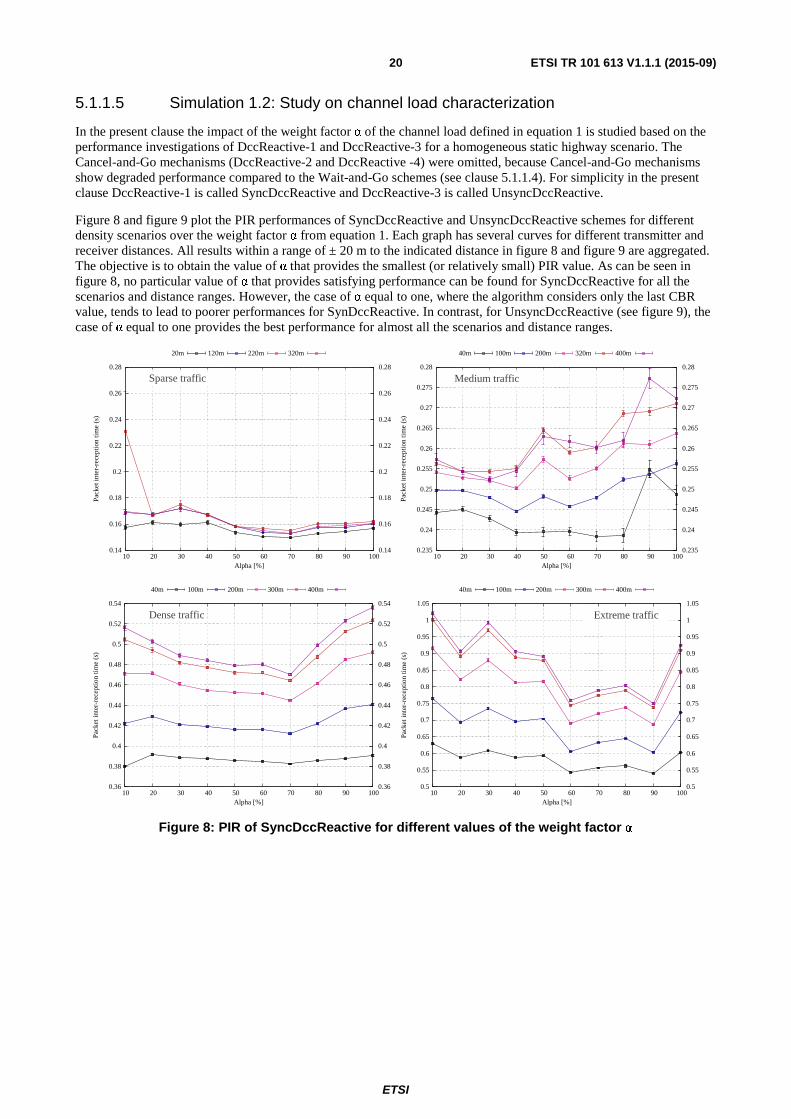
In the present clause the impact of the weight factor α of the channel load defined in equation 1 is studied based on the performance investigations of DccReactive-1 and DccReactive-3 for a homogeneous static highway scenario. The Cancel-and-Go mechanisms (DccReactive-2 and DccReactive -4) were omitted, because Cancel-and-Go mechanisms show degraded performance compared to the Wait-and-Go schemes (see clause 5.1.1.4). For simplicity in the present clause DccReactive-1 is called SyncDccReactive and DccReactive-3 is called UnsyncDccReactive.

Figure 8 and figure 9 plot the PIR performances of SyncDccReactive and UnsyncDccReactive schemes for different density scenarios over the weight factor α from equation 1. Each graph has several curves for different transmitter and receiver distances. All results within a range of ± 20 m to the indicated distance in figure 8 and figure 9 are aggregated. The objective is to obtain the value of α that provides the smallest (or relatively small) PIR value. As can be seen in figure 8, no particular value of α that provides satisfying performance can be found for SyncDccReactive for all the scenarios and distance ranges. However, the case of α equal to one, where the algorithm considers only the last CBR value, tends to lead to poorer performances for SynDccReactive. In contrast, for UnsyncDccReactive (see figure 9), the case of α equal to one provides the best performance for almost all the scenarios and distance ranges.

Figure 8: PIR of SyncDccReactive for different values of the weight factor α

0.14

0.16

0.18

0.2

0.22

0.24

0.26

0.28

10 20 30 40 50 60 70 80 90 100 0.14

0.16

0.18

0.2

0.22

0.24

0.26

0.28

Pac

ket i

nter

-rec

epti

on ti

me

(s)

Alpha [%]

20m 120m 220m 320m

0.235

0.24

0.245

0.25

0.255

0.26

0.265

0.27

0.275

0.28

10 20 30 40 50 60 70 80 90 100 0.235

0.24

0.245

0.25

0.255

0.26

0.265

0.27

0.275

0.28

Pac

ket i

nter

-rec

epti

on ti

me

(s)

Alpha [%]

40m 100m 200m 320m 400m

0.36

0.38

0.4

0.42

0.44

0.46

0.48

0.5

0.52

0.54

10 20 30 40 50 60 70 80 90 100 0.36

0.38

0.4

0.42

0.44

0.46

0.48

0.5

0.52

0.54

Pack

et in

ter-

rece

ptio

n ti

me

(s)

Alpha [%]

40m 100m 200m 300m 400m

0.5

0.55

0.6

0.65

0.7

0.75

0.8

0.85

0.9

0.95

1

1.05

10 20 30 40 50 60 70 80 90 100 0.5

0.55

0.6

0.65

0.7

0.75

0.8

0.85

0.9

0.95

1

1.05

Pack

et in

ter-

rece

ptio

n ti

me

(s)

Alpha [%]

40m 100m 200m 300m 400m

Sparse traffic Medium traffic

Dense traffic Extreme traffic

ETSI

ETSI TR 101 613 V1.1.1 (2015-09) 21

Figure 9: PIR of UnsyncDccReactive for different values of the weight factor α

Table 6 and table 7 list the weight factor α (see equation 1), which corresponds to the shortest PIR for SyncDccReactive (DccReactive_1) and UnsyncDccReactive (DccReactive_3) mechanisms. The difference of PIR between the minimum value and that for α = 1 is indicated for the cases where α is not equal to one. Table 6 clearly shows that for the synchronized DCC system, the best PIR performances are never achieved when α is equal to one; the difference between the minimum PIR and that for α equal to one is more than 10 ms. This implies that it is difficult to characterize the channel load using only the current CBR. In contrast, as table 7 shows, when the system is unsynchronized, the best PIR is achieved when α is equal to one. Hence, the channel load can be characterized by the current CBR only, when the system is unsynchronized. Note that when α equals 0,2 the PIR is shortest for small transmitter and receiver distances in the extreme scenario for UnsyncDccReactive, but the PIR difference between this minimum value and that for α = 1 is very small (4 ms).

Table 6: Weight factor α, which corresponds to the shortest PIR for SyncDccReactive

Scenario Distance between transmitter and receiver (m) 40 100 200 300 400

Medium 0,7

10 ms shorter than PIR (α = 1)

0,4 12 ms shorter

than PIR (α = 1)

0,4 13 ms shorter

than PIR (α = 1)

0,2 16 ms shorter

than PIR (α = 1)

0,3 20 ms shorter

than PIR (α = 1)

Dense 0,2


0,1 29 ms shorter

than PIR (α = 1)

0,7 47 ms shorter

than PIR (α = 1)

0,7 59 ms shorter

than PIR (α = 1)

0,7 66 ms shorter

than PIR (α = 1)

Extreme 0,1


0,9 12 ms shorter than

PIR (α = 1)


PIR (α = 1)


PIR (α = 1)


PIR (α = 1)

0.125

0.13

0.135

0.14

0.145

0.15

0.155

0.16

0.165

0.17

10 20 30 40 50 60 70 80 90 100 0.125

0.13

0.135

0.14

0.145

0.15

0.155

0.16

0.165

0.17

Pac

ket i

nter

-rec

eptio

n tim

e (s

)

Alpha [%]

20m 120m 220m 320m

0.19

0.2

0.21

0.22

0.23

0.24

0.25

0.26

10 20 30 40 50 60 70 80 90 100 0.19

0.2

0.21

0.22

0.23

0.24

0.25

0.26

Pac

ket i

nter

-rec

epti

on ti

me

(s)

Alpha [%]

40m 100m 200m 320m 400m

0.3

0.305

0.31

0.315

0.32

0.325

0.33

0.335

0.34

0.345

0.35

0.355

10 20 30 40 50 60 70 80 90 100 0.3

0.305

0.31

0.315

0.32

0.325

0.33

0.335

0.34

0.345

0.35

0.355

Pack

et in

ter-

rece

ptio

n tim

e (s

)

Alpha [%]

40m 100m 200m 300m 400m

0.48

0.5

0.52

0.54

0.56

0.58

0.6

0.62

0.64

10 20 30 40 50 60 70 80 90 100 0.48

0.5

0.52

0.54

0.56

0.58

0.6

0.62

0.64

Pac

ket i

nter

-rec

eptio

n tim

e (s

)

Alpha [%]

40m 100m 200m 300m 400m

Sparse traffic Medium traffic

Dense traffic Extreme traffic

ETSI

ETSI TR 101 613 V1.1.1 (2015-09) 22

Table 7: Weight factor α, which corresponds to the shortest PIR for UnsyncDccReactive

Scenario Transmitter and Receiver distance range (m) 40 100 200 300 400

Medium 1 1 1 1 1 Dense 1 1 1 1 1

Extreme 0,2 4 ms shorter than

that of α = 1

0,2 4 ms shorter than that of

α = 1

1 1 1

5.1.1.6 Simulation 1.3: Study on non-identical sensing capabilities

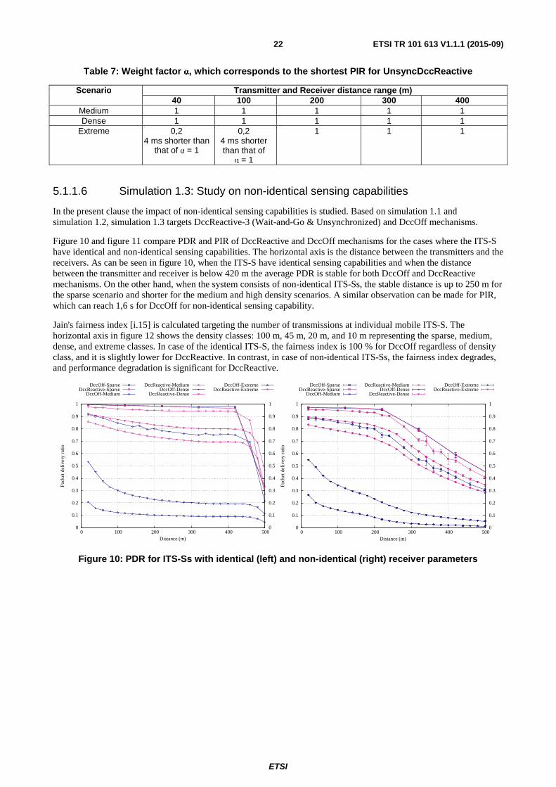
In the present clause the impact of non-identical sensing capabilities is studied. Based on simulation 1.1 and simulation 1.2, simulation 1.3 targets DccReactive-3 (Wait-and-Go & Unsynchronized) and DccOff mechanisms.

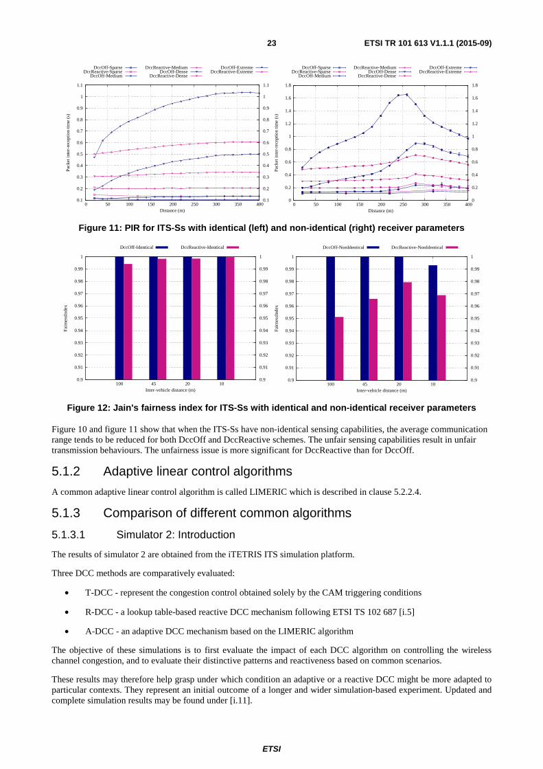
Figure 10 and figure 11 compare PDR and PIR of DccReactive and DccOff mechanisms for the cases where the ITS-S have identical and non-identical sensing capabilities. The horizontal axis is the distance between the transmitters and the receivers. As can be seen in figure 10, when the ITS-S have identical sensing capabilities and when the distance between the transmitter and receiver is below 420 m the average PDR is stable for both DccOff and DccReactive mechanisms. On the other hand, when the system consists of non-identical ITS-Ss, the stable distance is up to 250 m for the sparse scenario and shorter for the medium and high density scenarios. A similar observation can be made for PIR, which can reach 1,6 s for DccOff for non-identical sensing capability.

Jain's fairness index [i.15] is calculated targeting the number of transmissions at individual mobile ITS-S. The horizontal axis in figure 12 shows the density classes: 100 m, 45 m, 20 m, and 10 m representing the sparse, medium, dense, and extreme classes. In case of the identical ITS-S, the fairness index is 100 % for DccOff regardless of density class, and it is slightly lower for DccReactive. In contrast, in case of non-identical ITS-Ss, the fairness index degrades, and performance degradation is significant for DccReactive.

Figure 10: PDR for ITS-Ss with identical (left) and non-identical (right) receiver parameters

0

0.1

0.2

0.3

0.4

0.5

0.6

0.7

0.8

0.9

1

0 100 200 300 400 500 0

0.1

0.2

0.3

0.4

0.5

0.6

0.7

0.8

0.9

1

Pac

ket d

eliv

ery

rati

o

Distance (m)

DccOff-SparseDccReactive-Sparse

DccOff-Medium

DccReactive-MediumDccOff-Dense

DccReactive-Dense

DccOff-ExtremeDccReactive-Extreme

0

0.1

0.2

0.3

0.4

0.5

0.6

0.7

0.8

0.9

1

0 100 200 300 400 500 0

0.1

0.2

0.3

0.4

0.5

0.6

0.7

0.8

0.9

1

Pack

et d

eliv

ery

ratio

Distance (m)


DccOff-Medium


DccReactive-Dense


ETSI

ETSI TR 101 613 V1.1.1 (2015-09) 23

Figure 11: PIR for ITS-Ss with identical (left) and non-identical (right) receiver parameters

Figure 12: Jain's fairness index for ITS-Ss with identical and non-identical receiver parameters

Figure 10 and figure 11 show that when the ITS-Ss have non-identical sensing capabilities, the average communication range tends to be reduced for both DccOff and DccReactive schemes. The unfair sensing capabilities result in unfair transmission behaviours. The unfairness issue is more significant for DccReactive than for DccOff.

5.1.2 Adaptive linear control algorithms

A common adaptive linear control algorithm is called LIMERIC which is described in clause 5.2.2.4.

5.1.3 Comparison of different common algorithms


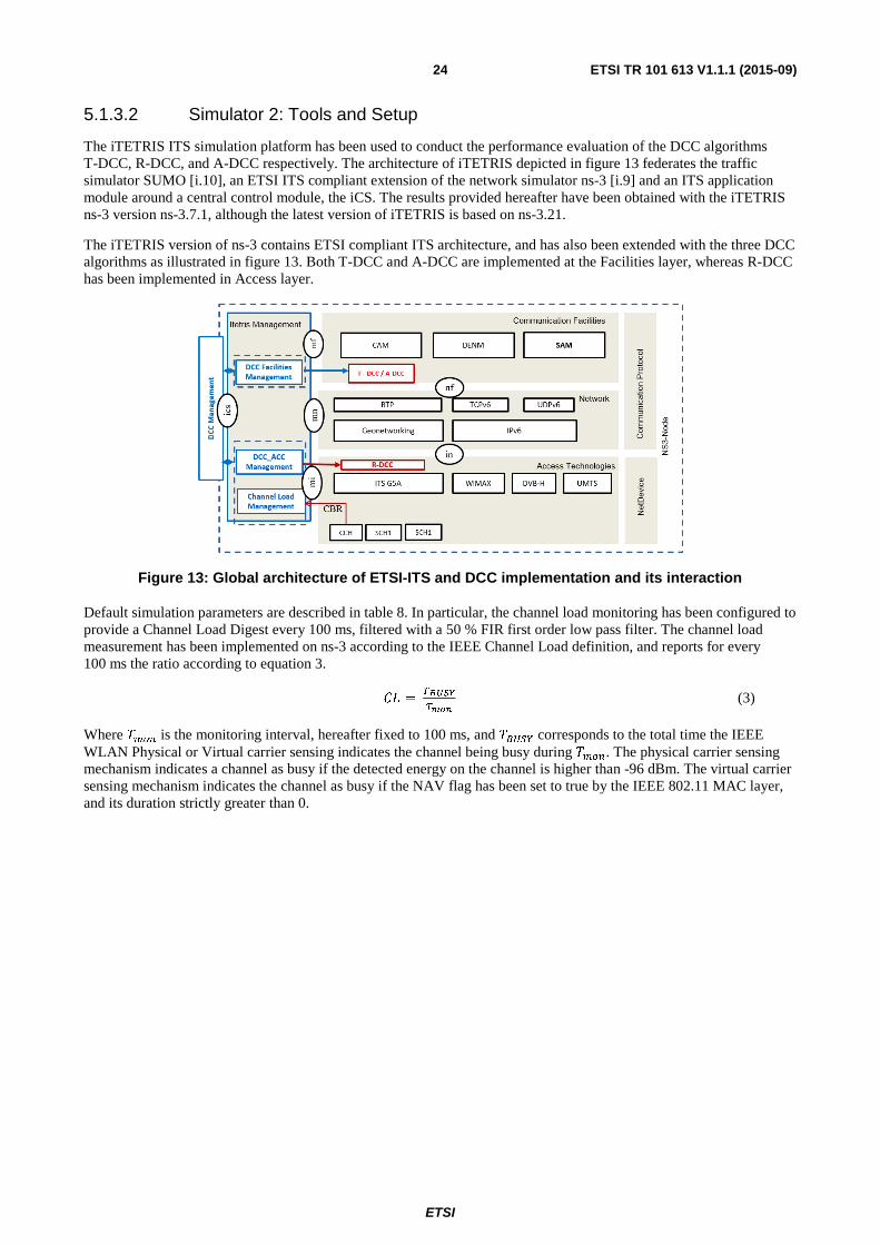
The results of simulator 2 are obtained from the iTETRIS ITS simulation platform.

Three DCC methods are comparatively evaluated:

• T-DCC - represent the congestion control obtained solely by the CAM triggering conditions

• R-DCC - a lookup table-based reactive DCC mechanism following ETSI TS 102 687 [i.5]

• A-DCC - an adaptive DCC mechanism based on the LIMERIC algorithm

The objective of these simulations is to first evaluate the impact of each DCC algorithm on controlling the wireless channel congestion, and to evaluate their distinctive patterns and reactiveness based on common scenarios.

These results may therefore help grasp under which condition an adaptive or a reactive DCC might be more adapted to particular contexts. They represent an initial outcome of a longer and wider simulation-based experiment. Updated and complete simulation results may be found under [i.11].

0.1

0.2

0.3

0.4

0.5

0.6

0.7

0.8

0.9

1

1.1

0 50 100 150 200 250 300 350 400 0.1

0.2

0.3

0.4

0.5

0.6

0.7

0.8

0.9

1

1.1

Pack

et in

ter-

rece

ptio

n tim

e (s

)

Distance (m)


DccOff-Medium


DccReactive-Dense


0

0.2

0.4

0.6

0.8

1

1.2

1.4

1.6

1.8

0 50 100 150 200 250 300 350 400 0

0.2

0.4

0.6

0.8

1

1.2

1.4

1.6

1.8

Pack

et in

ter-

rece

ptio

n ti

me

(s)

Distance (m)


DccOff-Medium


DccReactive-Dense


0.9

0.91

0.92

0.93

0.94

0.95

0.96

0.97

0.98

0.99

1

100 45 20 10 0.9

0.91

0.92

0.93

0.94

0.95

0.96

0.97

0.98

0.99

1

Fair

ness

Inde

x

Inter-vehicle distance (m)

DccOff-Identical DccReactive-Identical

0.9

0.91

0.92

0.93

0.94

0.95

0.96

0.97

0.98

0.99

1

100 45 20 10 0.9

0.91

0.92

0.93

0.94

0.95

0.96

0.97

0.98

0.99

1

Fair

ness

Inde

x

Inter-vehicle distance (m)

DccOff-NonIdentical DccReactive-NonIdentical

ETSI

ETSI TR 101 613 V1.1.1 (2015-09) 24

5.1.3.2 Simulator 2: Tools and Setup

The iTETRIS ITS simulation platform has been used to conduct the performance evaluation of the DCC algorithms T-DCC, R-DCC, and A-DCC respectively. The architecture of iTETRIS depicted in figure 13 federates the traffic simulator SUMO [i.10], an ETSI ITS compliant extension of the network simulator ns-3 [i.9] and an ITS application module around a central control module, the iCS. The results provided hereafter have been obtained with the iTETRIS ns-3 version ns-3.7.1, although the latest version of iTETRIS is based on ns-3.21.

The iTETRIS version of ns-3 contains ETSI compliant ITS architecture, and has also been extended with the three DCC algorithms as illustrated in figure 13. Both T-DCC and A-DCC are implemented at the Facilities layer, whereas R-DCC has been implemented in Access layer.

Figure 13: Global architecture of ETSI-ITS and DCC implementation and its interaction

Default simulation parameters are described in table 8. In particular, the channel load monitoring has been configured to provide a Channel Load Digest every 100 ms, filtered with a 50 % FIR first order low pass filter. The channel load measurement has been implemented on ns-3 according to the IEEE Channel Load definition, and reports for every 100 ms the ratio according to equation 3.

�� = ��

�� (3)

Where �� is the monitoring interval, hereafter fixed to 100 ms, and �� corresponds to the total time the IEEE WLAN Physical or Virtual carrier sensing indicates the channel being busy during ��. The physical carrier sensing mechanism indicates a channel as busy if the detected energy on the channel is higher than -96 dBm. The virtual carrier sensing mechanism indicates the channel as busy if the NAV flag has been set to true by the IEEE 802.11 MAC layer, and its duration strictly greater than 0.

ETSI

ETSI TR 101 613 V1.1.1 (2015-09) 25

Table 8: Default simulation parameters of simulator 2

Parameters Value Communication

CAM default TX rate 10 Hz CAM message size 300 Bytes

TX Power 23 dBm EDthreshold -96 dBm

EDCA Queue/TC 3 - CAM Modulation scheme QPSK ½ 6 Mbit/s

Antenna pattern Omnidirectional, gain = 1 dBi Access technology ITS G5A

ITS G5 Channel CCH Fading model LogDistance, exponent 2

Road network Lane width 3 m

Lanes in-flow 3 Lanes contra-flow 3

DCC parameters CBR monitor interval (Tmonitor) 100 ms

Monitoring Window (α) 0,5

Table 9 shows the R-DCC configuration lookup table, in particular the Toff values as function of the measured channel

load. From table 9 can be seen that R-DCC is actively controlling the channel load between 0 % and 59 %. Above 59 %, the channel load is only given by the message sizes and the number of ITS-S contributing to the channel, the Toff

value is fixed to 460 ms.

Although not described in details, the A-DCC has been configured with the same value for the target channel load of 60 %.

Table 9: Reactive DCC parameter lookup table used in simulator 2 for R-DCC

States CL (%) Toff (ms)

Relaxed 0 % ≤ CL < 19 % 60 Active_1 19 % ≤ CL < 27 % 100 Active_2 27 % ≤ CL < 35 % 180 Active_3 35 % ≤ CL < 43 % 260 Active_4 43 % ≤ CL < 51 % 340 Active_5 51 % ≤ CL < 59 % 420

Restricted CL ≥ 59 % 460

The vehicular traffic scenario is based on a LOS-F highway traffic condition as described in table 10. The central lane of the highway is equipped with static roadside ITS-S at a distance of 100 m each. The channel load will only be measured and averaged between all measuring static roadside ITS-S. To limit the border effects, only a 1 000 m central stretch to the 10 km total highway length is used for the channel load monitoring, and as such 10 roadside ITS-Ss are used to measure and average the channel load measurement.

In order to measure the reactiveness of DCC mechanisms to varying traffic conditions, a second traffic scenario has been configured, which contains LOS-F saturated traffic on one direction and clustered traffic conditions on the opposite direction. Each vehicle cluster corresponds to a LOS-F traffic condition, but the distance between clusters corresponds to a LOS-C traffic condition.

Table 10: Simulation scenario description

Category Objectives Scenario Mobility Performance criteria

1 Homogenous ITS-S density

2 Directions Dense traffic mobile Resilient

2 Variable Traffic One is dense and other is clustered clustered mobile Responsiveness

ETSI

ETSI TR 101 613 V1.1.1 (2015-09) 26

5.1.3.3 Simulator 2: Simulation results

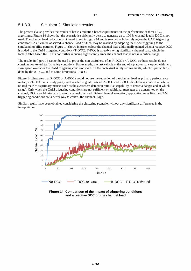
The present clause provides the results of basic simulation-based experiments on the performance of three DCC algorithms. Figure 14 shows that the scenario is sufficiently dense to generate up to 100 % channel load if DCC is not used. The channel load reduction is pictured in red in figure 14 and is reached only by relying on the CAM triggering conditions. As it can be observed, a channel load of 30 % may be reached by adapting the CAM triggering to the simulated mobility patterns. Figure 14 shows in green colour the channel load additionally gained when a reactive DCC is added to the CAM triggering conditions (T-DCC). T-DCC is already saving significant channel load, which the lookup table based R-DCC is not further reducing significantly since the channel load is not in a critical range.

The results in figure 14 cannot be used to prove the non-usefulness of an R-DCC or A-DCC, as these results do not consider contextual traffic safety conditions. For example, the last vehicle at the end of a platoon, all stopped with very slow speed overrides the CAM triggering conditions to fulfil the contextual safety requirements, which is particularly done by the A-DCC, and to some limitations R-DCC.

Figure 14 illustrates that R-DCC or A-DCC should not use the reduction of the channel load as primary performance metric, as T-DCC can already pretty well reach this goal. Instead, A-DCC and R-DCC should have contextual safety-related metrics as primary metric, such as the awareness detection ratio (i.e. capability to detect a danger and at which range). Only when the CAM triggering conditions are not sufficient or additional messages are transmitted on the channel, DCC should take care to avoid channel overload. Below channel saturation, application rules like the CAM triggering conditions are a better way to control the channel usage.

Similar results have been obtained considering the clustering scenario, without any significant differences in the interpretation.

Figure 14: Comparison of the impact of triggering conditions and a reactive DCC on the channel load

ETSI

ETSI TR 101 613 V1.1.1 (2015-09) 27

Figure 15: Comparison between A-DCC and R-DCC in terms of Channel Load for 10 Hz maximum CAM generation rate

In the next set of results, the performance of A-DCC and R-DCC in terms of channel load are compared, in particular their capabilities to stabilize the channel load at a target value. In figure 16, the blue curve shows that the A-DCC initially reaches a high channel load, before the adaptive component manages to reduce the load to the target channel load of 60 %. The orange curve represents the R-DCC, which converges faster to the channel load of 40 % , although being subject to significant initial oscillatory behavior. Figure 16 also shows that the adaptive approach uses the full amount of the available capacity, whereas the reactive approach only uses what is allowed by Toff from the lookup table.

Accordingly, A-DCC reaches a higher channel capacity usage, and as such, a higher refreshing rate between CAMs.

Figure 15 and figure 16 show that both A-DCC and R-DCC successfully manage to control the wireless congestion on a densely populated highway, which is the first requirement of a DCC algorithm. They also show that A-DCC uses all available capacity compared to R-DCC, which is expected to provide a higher packet reception rate and accordingly a better position awareness of other ITS-S. Resulting in a higher safety benefit for the C-ITS applications.

Figure 16: Comparison between A-DCC and R-DCC in terms of Channel Load for 5,56 Hz maximum CAM generation rate

ETSI

ETSI TR 101 613 V1.1.1 (2015-09) 28

5.2 Mixed use of different algorithms

5.2.1 Simulator 3: Conclusions

With simulator 3, coexistence of a reactive table-based DCC algorithm called CAM-DCC and LIMERIC [i.16], [i.17] has been studied. Firstly, it is observed that introducing LIMERIC vehicle ITS-S in a CAM-DCC network leads to only modest performance degradations of CAM-DCC in one of the test scenarios (Simulation Y.2), and can improve the performance of the day 1 deployed CAM-DCC vehicle ITS-S in the rest of the scenarios. The improvement might be largely due to inefficiencies of the CAM-DCC algorithm when implemented with synchronized channel load measurements.

Secondly, it is demonstrated that the magnitude of the performance impact of LIMERIC on CAM-DCC can be controlled through adjustments in LIMERIC target Channel Busy Percentage (CBP) and/or CAM-DCC look-up table parameters. These adjustments affect the performance difference in terms of packet error rate and 95th percentile inter-packet gap. In the simulation scenario, a decreased LIMERIC target CBP can reduce the performance difference between CAM-DCC and LIMERIC vehicle ITS-S. Further, the modified CAM-DCC look-up table also led to a decreased difference.

Thirdly, it is observed that a high degree of fairness can be achieved through careful selection of the LIMERIC target CBP parameter and the CAM-DCC look-up table parameters. With parameter changes in both LIMERIC and CAM-DCC it was possible to achieve close agreement between LIMERIC and CAM-DCC transmitters in terms of the packet error rates and 95th percentile inter packet gap metrics. It is believed that the exact table values for CAM-DCC, and/or exact target CBP value for LIMERIC, depends on the density of vehicles. However, this first study on co-existence between CAM-DCC and LIMERIC vehicle ITS-S looks very promising since none of the algorithms suffer from major performance degradation.

5.2.2 Simulator 3: Introduction

5.2.2.1 Overview

The Medium Access Control (MAC) and Physical Layer (PHY) protocols for vehicular communications are specified in the IEEE 802.11-2012 [i.3] standard and well accepted. Differences exist, however, in other components. In particular, several congestion control algorithms are under investigation to improve packet error rate (PER) and inter-packet gap (IPG) performance at higher densities of vehicles, where interference challenges exist. It is expected that the standards for congestion control algorithms differ across regions. Two representative algorithms are the Decentralized Congestion Control (CAM-DCC) framework defined in 2011 by the European Telecommunication Standards Institute (ETSI) [i.5] and the LIMERIC linear control algorithm [i.17] originally proposed for use in the U.S.

With different algorithms likely to be deployed, situations could arise where vehicle ITS-S with different algorithms operate in the same network. Such a network is referred as a mixed network. While each geographic region is likely to mandate a specific algorithm, several possible reasons for mixed networks exist. First, there may be a desire for moving to a common algorithm eventually, which would require that any newly deployed vehicle can co-exist with vehicle ITS-S using the legacy algorithm. Second, vehicle manufacturers often prefer to minimize differences in their models across regions and may ask permission to deliver vehicle ITS-S with their "standard" algorithm to regions initially using a different algorithm. Third, vehicle ITS-S with a different algorithm may be accidentally introduced into a region, perhaps through illegal imports.

In the present clause, the performance impact of such mixed network operation and techniques to reduce undesirable effects are studied. In particular, the analysis investigates a scenario in which CAM-DCC is deployed for day one applications and LIMERIC is introduced afterwards. Given such a mixed network with coexisting CAM-DCC and LIMERIC vehicle ITS-S, the following questions raise:

• Do the CAM-DCC vehicle ITS-S experience performance changes after LIMERIC vehicle ITS-S are introduced into the network? Does LIMERIC show a similar performance as CAM-DCC?

• If an undesirable performance difference does exist, how can it be reduced?

ETSI

ETSI TR 101 613 V1.1.1 (2015-09) 29

To address these questions, simulations using the ns-2.34 network simulator [i.9] have been conducted. In these simulations, the percentage of LIMERIC vehicle ITS-S in the mixed network starts at 0 % (a network with all vehicles running CAM-DCC) and increases up to 100 % (a network with all vehicle ITS-S running LIMERIC) in order to investigate the performance impact. Simulations are also executed with different LIMERIC target rate and CAM-DCC lookup table parameter settings to study the impact of these adjustments on the algorithm performance and their effectiveness in reducing the performance difference between the algorithms.

5.2.2.2 DCC background

Most vehicular network applications require frequent exchange of status messages among vehicle ITS-S, which inform neighbours about vehicle positions and movements. These messages are referred to as Cooperative Awareness Messages (CAMs) in Europe (specified in ETSI EN 302 637-2 [i.6]) and Basic Safety Messages (BSM) in the US. Such messages are transmitted multiple times per second and when many vehicle ITS-S enter the same area, the total volume of messages can lead to channel congestion and excessive adjacent channel interference. The congestion control algorithms therefore aim to reduce the frequency of message transmissions when vehicle density becomes too high. To achieve this, the algorithms specify when messages can be generated and when they can be sent to the MAC layer for transmission.

5.2.2.3 CAM-DCC algorithm

When using DCC for controlling the radio channel congestion, it does not only shape the traffic into the MAC layer, but also limits CAM generation in the facilities layer. Therefore, the DCC algorithm with CAM generation is referred to as CAM-DCC in the present clause 5.2. The CAM generation rules and DCC mechanisms are described in the following paragraph. The CAM generation has been implemented in simulator 3 according to ETSI EN 302 637-2 [i.6].

The specific generation times of CAMs are determined by DCC and vehicle dynamics, with a constraint that the time interval between two consecutive generated CAMs should be no less than 100 ms and no more than 1 000 ms. Generally, a new CAM is expected to be generated when the following two conditions are met:

• The elapsed time since the last CAM generation is larger than the message interval, which is provided by DCC through the parameter T_GenCam_DCC

• One of the following vehicle dynamics criteria are met:

1) heading changed > 4°;

2) position changed > 4 m;

3) magnitude of speed changed > 0,5 m/s.

If the above two conditions are not met for one second after the last CAM generation, a CAM is generated immediately. When a CAM is generated due to one of these dynamics criteria, a second and third (the actual number is controlled by N_GenCam, the maximum value of N_GenCam defined in ETSI EN 302 637-2 [i.6] is 3) CAM are generated at the same interval unless the changing dynamics lead to a shorter interval.

CAM-DCC receives generated CAMs and regulates their transmission time using a state machine, which distinguishes between three main states: RELAXED, ACTIVE, and RESTRICTIVE, see ETSI TS 102 687 [i.5]. The ACTIVE state can be further divided into several sub-states. Each state (sub-state) defines a set of transmission parameters (e.g. transmission rate, transmission power, data rate), which controls the transmission behaviours. The transition between different states is driven by the channel load (CL), locally measured by each ITS-S during a sampling interval. In simulator 3, the CL is indicated by the CBP, which is the fraction of time during which the channel is measured as busy. NDL_MinChannelLoad is the minimum CL below which the channel is practically free and the DCC state is RELAXED. While NDL_MaxChannelLoad is the maximum CL above which the channel is considered to be overloaded and the DCC state is RESTRICTIVE. A transition from RELAXED to ACTIVE and from ACTIVE to RESTRICTIVE is allowed if the minimum CL measured over the last NDL_TimeUp period is higher than NDL_MinChannelLoad and NDL_MaxChannelLoad, respectively. Similarly, a transition from RESTRICTIVE to ACTIVE and from ACTIVE to RELAEXED occurs if the maximum CL measured over the last NDL_TimeDown period is lower than NDL_MinChannelLoad and NDL_MaxChannelLoad, respectively.

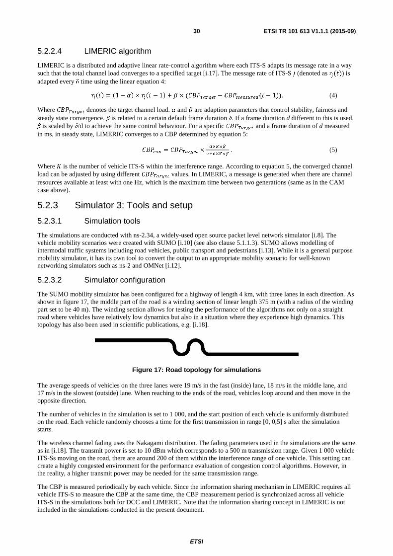
ETSI

ETSI TR 101 613 V1.1.1 (2015-09) 30

5.2.2.4 LIMERIC algorithm

LIMERIC is a distributed and adaptive linear rate-control algorithm where each ITS-S adapts its message rate in a way such that the total channel load converges to a specified target [i.17]. The message rate of ITS-S � (denoted as �(�)) is adapted every δ time using the linear equation 4:

�� = �1 − × �� − 1 + � × (�� − ��(� − 1)). (4)

Where �� denotes the target channel load. � and � are adaption parameters that control stability, fairness and steady state convergence. β is related to a certain default frame duration δ. If a frame duration d different to this is used, β is scaled by δ/d to achieve the same control behaviour. For a specific ��and a frame duration of d measured in ms, in steady state, LIMERIC converges to a CBP determined by equation 5:

�� = �� ××�×�

��×�×� . (5)

Where � is the number of vehicle ITS-S within the interference range. According to equation 5, the converged channel load can be adjusted by using different �� values. In LIMERIC, a message is generated when there are channel resources available at least with one Hz, which is the maximum time between two generations (same as in the CAM case above).

5.2.3 Simulator 3: Tools and setup

5.2.3.1 Simulation tools

The simulations are conducted with ns-2.34, a widely-used open source packet level network simulator [i.8]. The vehicle mobility scenarios were created with SUMO [i.10] (see also clause 5.1.1.3). SUMO allows modelling of intermodal traffic systems including road vehicles, public transport and pedestrians [i.13]. While it is a general purpose mobility simulator, it has its own tool to convert the output to an appropriate mobility scenario for well-known networking simulators such as ns-2 and OMNet [i.12].

5.2.3.2 Simulator configuration

The SUMO mobility simulator has been configured for a highway of length 4 km, with three lanes in each direction. As shown in figure 17, the middle part of the road is a winding section of linear length 375 m (with a radius of the winding part set to be 40 m). The winding section allows for testing the performance of the algorithms not only on a straight road where vehicles have relatively low dynamics but also in a situation where they experience high dynamics. This topology has also been used in scientific publications, e.g. [i.18].

Figure 17: Road topology for simulations

The average speeds of vehicles on the three lanes were 19 m/s in the fast (inside) lane, 18 m/s in the middle lane, and 17 m/s in the slowest (outside) lane. When reaching to the ends of the road, vehicles loop around and then move in the opposite direction.

The number of vehicles in the simulation is set to 1 000, and the start position of each vehicle is uniformly distributed on the road. Each vehicle randomly chooses a time for the first transmission in range [0, 0,5] s after the simulation starts.

The wireless channel fading uses the Nakagami distribution. The fading parameters used in the simulations are the same as in [i.18]. The transmit power is set to 10 dBm which corresponds to a 500 m transmission range. Given 1 000 vehicle ITS-Ss moving on the road, there are around 200 of them within the interference range of one vehicle. This setting can create a highly congested environment for the performance evaluation of congestion control algorithms. However, in the reality, a higher transmit power may be needed for the same transmission range.

The CBP is measured periodically by each vehicle. Since the information sharing mechanism in LIMERIC requires all vehicle ITS-S to measure the CBP at the same time, the CBP measurement period is synchronized across all vehicle ITS-S in the simulations both for DCC and LIMERIC. Note that the information sharing concept in LIMERIC is not included in the simulations conducted in the present document.

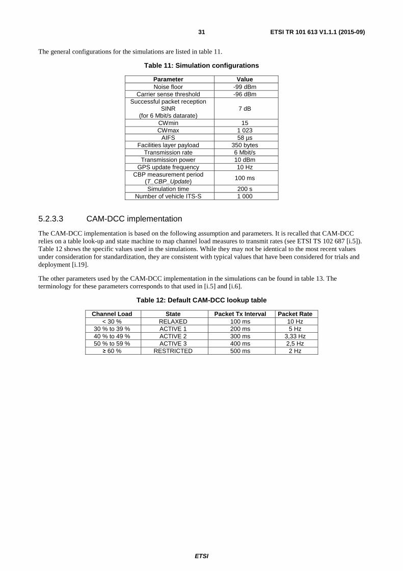
ETSI

ETSI TR 101 613 V1.1.1 (2015-09) 31

The general configurations for the simulations are listed in table 11.

Table 11: Simulation configurations

Parameter Value Noise floor -99 dBm

Carrier sense threshold -96 dBm Successful packet reception

SINR (for 6 Mbit/s datarate)

7 dB

CWmin 15 CWmax 1 023

AIFS 58 µs Facilities layer payload 350 bytes

Transmission rate 6 Mbit/s Transmission power 10 dBm

GPS update frequency 10 Hz CBP measurement period

(T_CBP_Update) 100 ms

Simulation time 200 s Number of vehicle ITS-S 1 000

5.2.3.3 CAM-DCC implementation

The CAM-DCC implementation is based on the following assumption and parameters. It is recalled that CAM-DCC relies on a table look-up and state machine to map channel load measures to transmit rates (see ETSI TS 102 687 [i.5]). Table 12 shows the specific values used in the simulations. While they may not be identical to the most recent values under consideration for standardization, they are consistent with typical values that have been considered for trials and deployment [i.19].

The other parameters used by the CAM-DCC implementation in the simulations can be found in table 13. The terminology for these parameters corresponds to that used in [i.5] and [i.6].

Table 12: Default CAM-DCC lookup table

Channel Load State Packet Tx Interval Packet Rate < 30 % RELAXED 100 ms 10 Hz

30 % to 39 % ACTIVE 1 200 ms 5 Hz 40 % to 49 % ACTIVE 2 300 ms 3,33 Hz 50 % to 59 % ACTIVE 3 400 ms 2,5 Hz

≥ 60 % RESTRICTED 500 ms 2 Hz

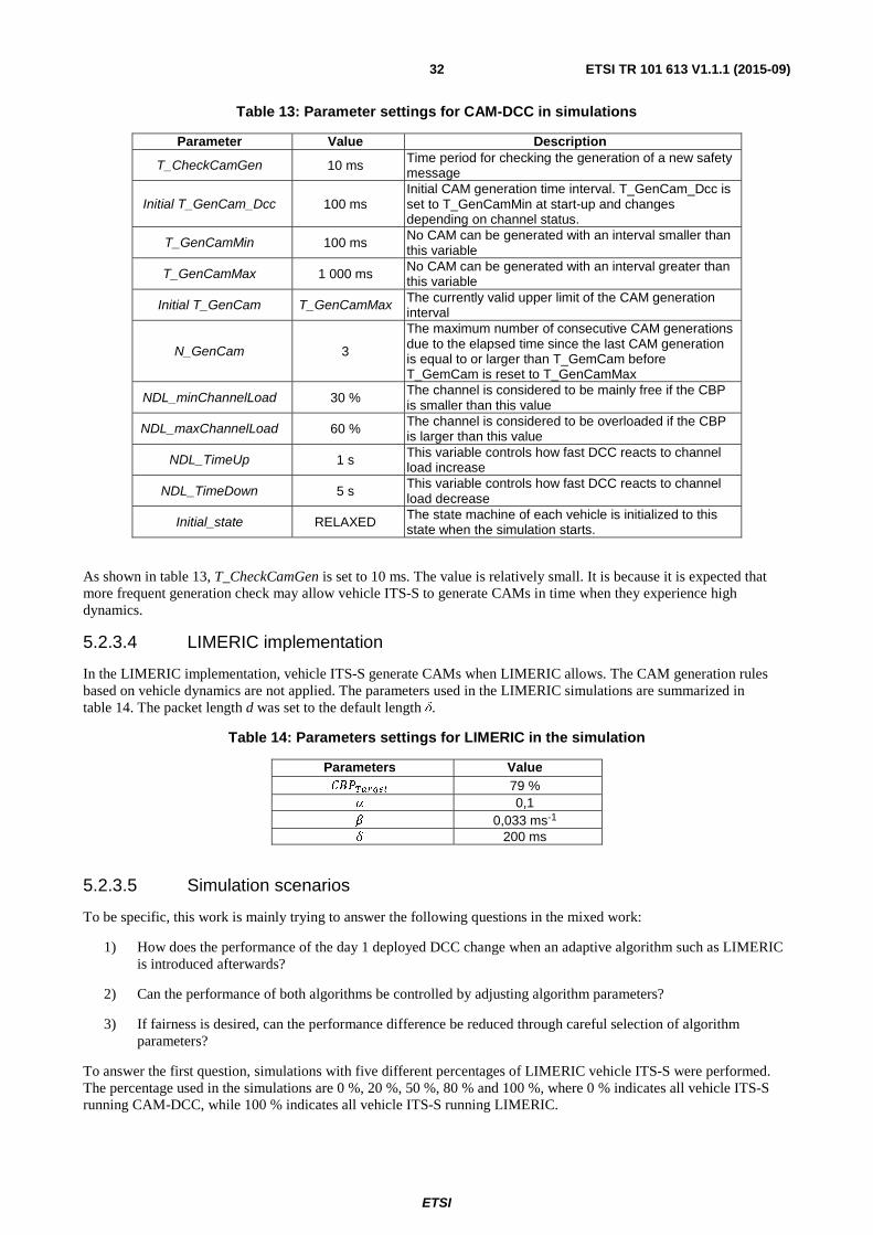
ETSI

ETSI TR 101 613 V1.1.1 (2015-09) 32

Table 13: Parameter settings for CAM-DCC in simulations

Parameter Value Description

T_CheckCamGen 10 ms Time period for checking the generation of a new safety message

Initial T_GenCam_Dcc 100 ms Initial CAM generation time interval. T_GenCam_Dcc is set to T_GenCamMin at start-up and changes depending on channel status.

T_GenCamMin 100 ms No CAM can be generated with an interval smaller than this variable

T_GenCamMax 1 000 ms No CAM can be generated with an interval greater than this variable

Initial T_GenCam T_GenCamMax The currently valid upper limit of the CAM generation interval

N_GenCam 3

The maximum number of consecutive CAM generations due to the elapsed time since the last CAM generation is equal to or larger than T_GemCam before T_GemCam is reset to T_GenCamMax

NDL_minChannelLoad 30 % The channel is considered to be mainly free if the CBP is smaller than this value

NDL_maxChannelLoad 60 % The channel is considered to be overloaded if the CBP is larger than this value

NDL_TimeUp 1 s This variable controls how fast DCC reacts to channel load increase

NDL_TimeDown 5 s This variable controls how fast DCC reacts to channel load decrease

Initial_state RELAXED The state machine of each vehicle is initialized to this state when the simulation starts.

As shown in table 13, T_CheckCamGen is set to 10 ms. The value is relatively small. It is because it is expected that more frequent generation check may allow vehicle ITS-S to generate CAMs in time when they experience high dynamics.

5.2.3.4 LIMERIC implementation

In the LIMERIC implementation, vehicle ITS-S generate CAMs when LIMERIC allows. The CAM generation rules based on vehicle dynamics are not applied. The parameters used in the LIMERIC simulations are summarized in table 14. The packet length d was set to the default length δ.

Table 14: Parameters settings for LIMERIC in the simulation

Parameters Value �� 79 %

� 0,1 � 0,033 ms-1

� 200 ms

5.2.3.5 Simulation scenarios

To be specific, this work is mainly trying to answer the following questions in the mixed work:

1) How does the performance of the day 1 deployed DCC change when an adaptive algorithm such as LIMERIC is introduced afterwards?

2) Can the performance of both algorithms be controlled by adjusting algorithm parameters?

3) If fairness is desired, can the performance difference be reduced through careful selection of algorithm parameters?

To answer the first question, simulations with five different percentages of LIMERIC vehicle ITS-S were performed. The percentage used in the simulations are 0 %, 20 %, 50 %, 80 % and 100 %, where 0 % indicates all vehicle ITS-S running CAM-DCC, while 100 % indicates all vehicle ITS-S running LIMERIC.

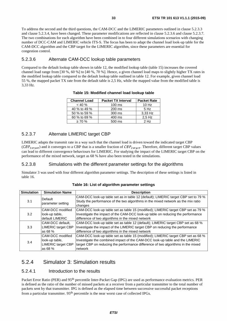
ETSI

ETSI TR 101 613 V1.1.1 (2015-09) 33

To address the second and the third questions, the CAM-DCC and the LIMERIC parameters outlined in clause 5.2.3.3 and clause 5.2.3.4, have been changed. These parameter modifications are reflected in clause 5.2.3.6 and clause 5.2.3.7. The two combinations for each algorithm have been combined in to four different simulations scenarios with changing number of DCC-CAM and LIMERIC vehicle ITS-S. The focus has been to adapt the channel load look-up table for the CAM-DCC algorithm and the CBP target for the LIMERIC algorithm, since these parameters are essential for congestion control.

5.2.3.6 Alternate CAM-DCC lookup table parameters

Compared to the default lookup table shown in table 12, the modified lookup table (table 15) increases the covered channel load range from [30 %, 60 %] to [40 %, 70 %]. Hence, a given channel load maps to slightly higher TX rates in the modified lookup table compared to the default lookup table outlined in table 12. For example, given channel load 55 %, the mapped packet TX rate from the default table is 2,5 Hz, while the mapped value from the modified table is 3,33 Hz.

Table 15: Modified channel load lookup table

Channel Load Packet TX Interval Packet Rate < 40 % 100 ms 10 Hz

40 % to 49 % 200 ms 5 Hz 50 % to 59 % 300 ms 3,33 Hz 60 % to 69 % 400 ms 2,5 Hz

≥ 70 % 500 ms 2 Hz

5.2.3.7 Alternate LIMERIC target CBP

LIMERIC adapts the transmit rate in a way such that the channel load is driven toward the indicated target CBP (��) and it converges to a CBP that is a smaller fraction of ��. Therefore, different target CBP values can lead to different convergence behaviours for LIMERIC. For studying the impact of the LIMERIC target CBP on the performance of the mixed network, target as 68 % have also been tested in the simulations.

5.2.3.8 Simulations with the different parameter settings for the algorithms

Simulator 3 was used with four different algorithm parameter settings. The description of these settings is listed in table 16.

Table 16: List of algorithm parameter settings

Simulation Simulation Name Description

3.1 Default parameter setting

CAM-DCC look-up table set as in table 12 (default); LIMERIC target CBP set to 79 % Study the performance of the two algorithms in the mixed network as the mix ratio changes

3.2 CAM-DCC modified look-up table, default LIMERIC

CAM-DCC look-up table set as table 15 (modified); LIMERIC target CBP set as 79 % Investigate the impact of the CAM-DCC look-up table on reducing the performance difference of two algorithms in the mixed network

3.3 CAM-DCC default, LIMERIC target CBP as 68 %

CAM-DCC look-up table set as table 12 (default); LIMERIC target CBP set as 68 % Investigate the impact of the LIMERIC target CBP on reducing the performance difference of two algorithms in the mixed network

3.4

CAM-DCC modified look-up table, LIMERIC target CBP as 68 %

CAM-DCC look-up table set as table 15 (modified); LIMERIC target CBP set as 68 % Investigate the combined impact of the CAM-DCC look-up table and the LIMERIC target CBP on reducing the performance difference of two algorithms in the mixed network

5.2.4 Simulator 3: Simulation results

5.2.4.1 Introduction to the results

Packet Error Ratio (PER) and 95th percentile Inter-Packet Gap (IPG) are used as performance evaluation metrics. PER is defined as the ratio of the number of missed packets at a receiver from a particular transmitter to the total number of packets sent by that transmitter. IPG is defined as the elapsed time between successive successful packet receptions from a particular transmitter. 95th percentile is the near worst case of collected IPGs.

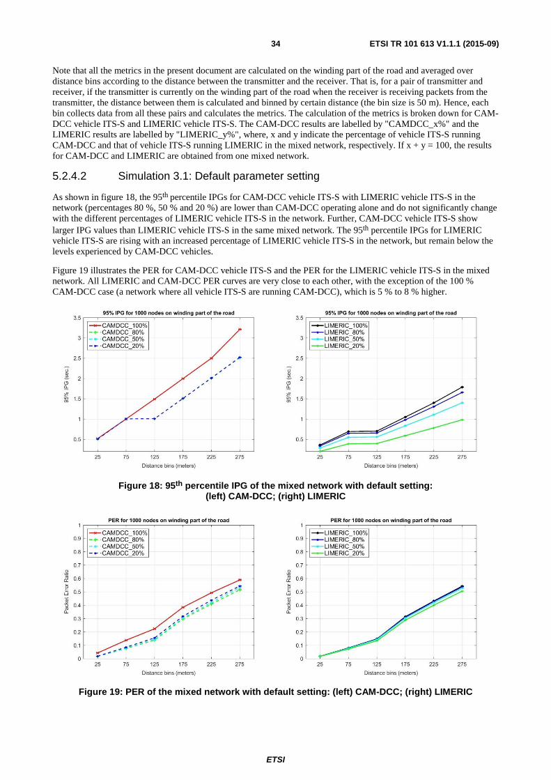
ETSI

ETSI TR 101 613 V1.1.1 (2015-09) 34

Note that all the metrics in the present document are calculated on the winding part of the road and averaged over distance bins according to the distance between the transmitter and the receiver. That is, for a pair of transmitter and receiver, if the transmitter is currently on the winding part of the road when the receiver is receiving packets from the transmitter, the distance between them is calculated and binned by certain distance (the bin size is 50 m). Hence, each bin collects data from all these pairs and calculates the metrics. The calculation of the metrics is broken down for CAM-DCC vehicle ITS-S and LIMERIC vehicle ITS-S. The CAM-DCC results are labelled by "CAMDCC_x%" and the LIMERIC results are labelled by "LIMERIC_y%", where, x and y indicate the percentage of vehicle ITS-S running CAM-DCC and that of vehicle ITS-S running LIMERIC in the mixed network, respectively. If x + y = 100, the results for CAM-DCC and LIMERIC are obtained from one mixed network.

5.2.4.2 Simulation 3.1: Default parameter setting

As shown in figure 18, the 95th percentile IPGs for CAM-DCC vehicle ITS-S with LIMERIC vehicle ITS-S in the network (percentages 80 %, 50 % and 20 %) are lower than CAM-DCC operating alone and do not significantly change with the different percentages of LIMERIC vehicle ITS-S in the network. Further, CAM-DCC vehicle ITS-S show larger IPG values than LIMERIC vehicle ITS-S in the same mixed network. The 95th percentile IPGs for LIMERIC vehicle ITS-S are rising with an increased percentage of LIMERIC vehicle ITS-S in the network, but remain below the levels experienced by CAM-DCC vehicles.

Figure 19 illustrates the PER for CAM-DCC vehicle ITS-S and the PER for the LIMERIC vehicle ITS-S in the mixed network. All LIMERIC and CAM-DCC PER curves are very close to each other, with the exception of the 100 % CAM-DCC case (a network where all vehicle ITS-S are running CAM-DCC), which is 5 % to 8 % higher.

Figure 18: 95th percentile IPG of the mixed network with default setting: (left) CAM-DCC; (right) LIMERIC

Figure 19: PER of the mixed network with default setting: (left) CAM-DCC; (right) LIMERIC

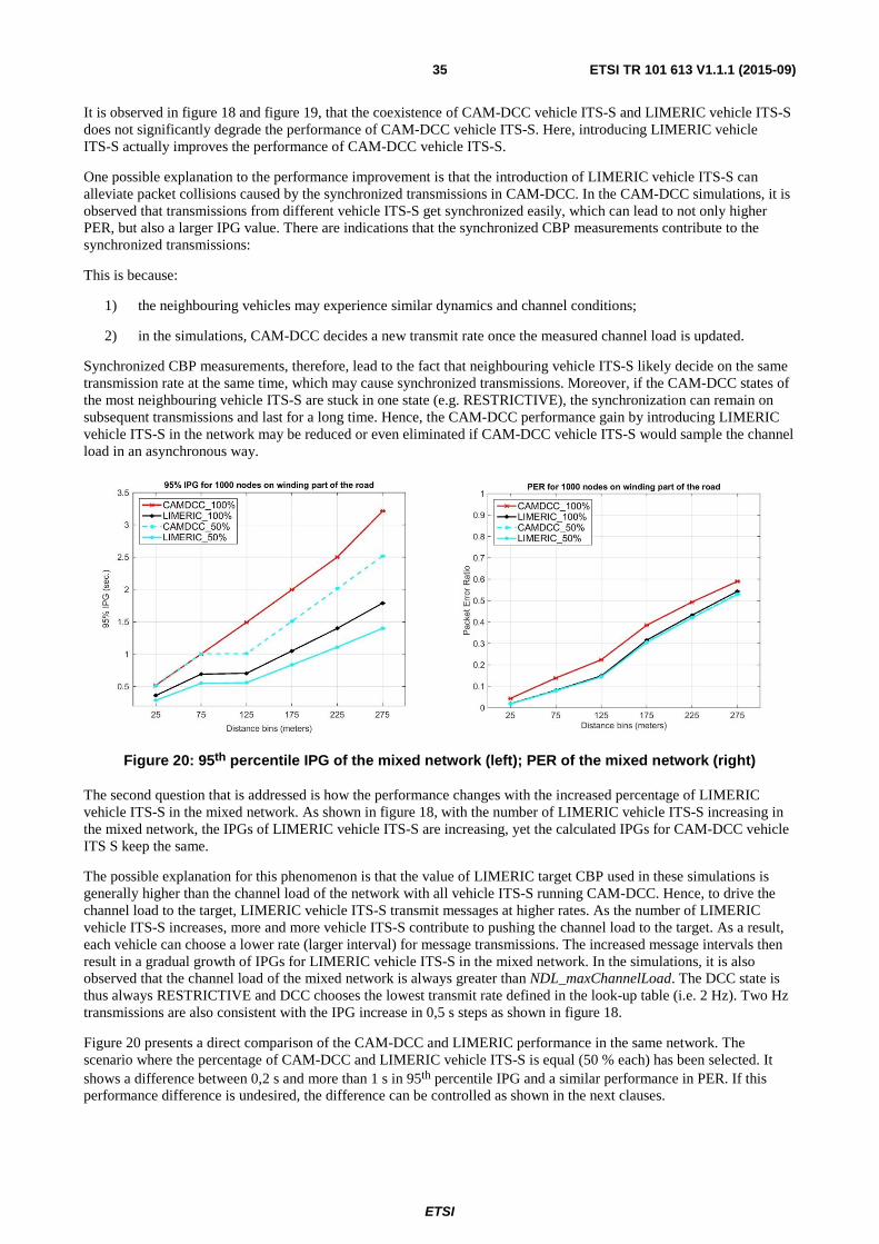
ETSI

ETSI TR 101 613 V1.1.1 (2015-09) 35

It is observed in figure 18 and figure 19, that the coexistence of CAM-DCC vehicle ITS-S and LIMERIC vehicle ITS-S does not significantly degrade the performance of CAM-DCC vehicle ITS-S. Here, introducing LIMERIC vehicle ITS-S actually improves the performance of CAM-DCC vehicle ITS-S.

One possible explanation to the performance improvement is that the introduction of LIMERIC vehicle ITS-S can alleviate packet collisions caused by the synchronized transmissions in CAM-DCC. In the CAM-DCC simulations, it is observed that transmissions from different vehicle ITS-S get synchronized easily, which can lead to not only higher PER, but also a larger IPG value. There are indications that the synchronized CBP measurements contribute to the synchronized transmissions:

This is because:

1) the neighbouring vehicles may experience similar dynamics and channel conditions;

2) in the simulations, CAM-DCC decides a new transmit rate once the measured channel load is updated.

Synchronized CBP measurements, therefore, lead to the fact that neighbouring vehicle ITS-S likely decide on the same transmission rate at the same time, which may cause synchronized transmissions. Moreover, if the CAM-DCC states of the most neighbouring vehicle ITS-S are stuck in one state (e.g. RESTRICTIVE), the synchronization can remain on subsequent transmissions and last for a long time. Hence, the CAM-DCC performance gain by introducing LIMERIC vehicle ITS-S in the network may be reduced or even eliminated if CAM-DCC vehicle ITS-S would sample the channel load in an asynchronous way.

Figure 20: 95th percentile IPG of the mixed network (left); PER of the mixed network (right)

The second question that is addressed is how the performance changes with the increased percentage of LIMERIC vehicle ITS-S in the mixed network. As shown in figure 18, with the number of LIMERIC vehicle ITS-S increasing in the mixed network, the IPGs of LIMERIC vehicle ITS-S are increasing, yet the calculated IPGs for CAM-DCC vehicle ITS S keep the same.

The possible explanation for this phenomenon is that the value of LIMERIC target CBP used in these simulations is generally higher than the channel load of the network with all vehicle ITS-S running CAM-DCC. Hence, to drive the channel load to the target, LIMERIC vehicle ITS-S transmit messages at higher rates. As the number of LIMERIC vehicle ITS-S increases, more and more vehicle ITS-S contribute to pushing the channel load to the target. As a result, each vehicle can choose a lower rate (larger interval) for message transmissions. The increased message intervals then result in a gradual growth of IPGs for LIMERIC vehicle ITS-S in the mixed network. In the simulations, it is also observed that the channel load of the mixed network is always greater than NDL_maxChannelLoad. The DCC state is thus always RESTRICTIVE and DCC chooses the lowest transmit rate defined in the look-up table (i.e. 2 Hz). Two Hz transmissions are also consistent with the IPG increase in 0,5 s steps as shown in figure 18.

Figure 20 presents a direct comparison of the CAM-DCC and LIMERIC performance in the same network. The scenario where the percentage of CAM-DCC and LIMERIC vehicle ITS-S is equal (50 % each) has been selected. It shows a difference between 0,2 s and more than 1 s in 95th percentile IPG and a similar performance in PER. If this performance difference is undesired, the difference can be controlled as shown in the next clauses.

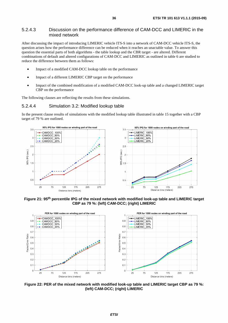
ETSI

ETSI TR 101 613 V1.1.1 (2015-09) 36

5.2.4.3 Discussion on the performance difference of CAM-DCC and LIMERIC in the mixed network

After discussing the impact of introducing LIMERIC vehicle ITS-S into a network of CAM-DCC vehicle ITS-S, the question arises how the performance difference can be reduced when it reaches an unactable value. To answer this question the essential parts of both algorithms - the table lookup and the CBR target - are altered. Different combinations of default and altered configurations of CAM-DCC and LIMERIC as outlined in table 6 are studied to reduce the difference between them as follows:

• Impact of a modified CAM-DCC lookup table on the performance

• Impact of a different LIMERIC CBP target on the performance

• Impact of the combined modification of a modified CAM-DCC look-up table and a changed LIMERIC target CBP on the performance

The following clauses are reflecting the results from these simulations.

5.2.4.4 Simulation 3.2: Modified lookup table

In the present clause results of simulations with the modified lookup table illustrated in table 15 together with a CBP target of 79 % are outlined.

Figure 21: 95th percentile IPG of the mixed network with modified look-up table and LIMERIC target CBP as 79 %: (left) CAM-DCC; (right) LIMERIC

Figure 22: PER of the mixed network with modified look-up table and LIMERIC target CBP as 79 %: (left) CAM-DCC; (right) LIMERIC

ETSI

ETSI TR 101 613 V1.1.1 (2015-09) 37

As shown in the left plot of figure 21, the introduction of LIMERIC vehicle ITS-S results in an increase in IPG for CAM-DCC vehicle ITS-S. This is mainly because: in the simulation where all vehicle ITS-S are running CAM-DCC, the channel loads measured by the most of vehicles located on the winding part of the road varies from 61 % to 69 %. Given this range of the CBP, the mapped transmit rate from the modified lookup table is 2,5 Hz. However, as LIMERIC vehicle ITS-S are introduced into the network, the channel loads have been driven to a higher level due to the high CBP target (i.e. 79 %) of LIMERIC. The mapped transmit rate of the increased channel load is 2 Hz. A higher transmit rate uses a lower message interval, which can further lead to a lower IPG. This may explain why IPG values of CAM-DCC vehicle ITS-S increase after LIMERIC vehicle ITS-S are introduced into the network. Figure 22 shows a similar trend: the PER is increased by 2 % on average after LIMERIC vehicle ITS-S are introduced. The reason may be the modified look-up table helps to reduce the possibility that the transmissions get synchronized. The synchronized transmission issue identified in the previous section is alleviated to a large extent. Normally, a lower channel load corresponds to a lower PER. Thus, the simulation with all vehicle ITS-S running CAM-DCC shows a smaller PER due to the comparatively lower CBP.

As depicted in figure 23, the modified lookup table cannot reduce the performance difference of two algorithms in the mixed network. This may be because in both simulations, where the default lookup table and the modified table are used respectively, DCC operates in RESTRICTIVE state in both cases and LIMERIC converges to one CBP value using similar rates in both cases.

Figure 23: 95th percentile IPG of the mixed network with different CAM-DCC look-up table: (left) default look-up table; (right) modified look-up table

5.2.4.5 Simulation 3.3: Modified LIMERIC target value

In the present clause, results of simulations with the default lookup table, illustrated in table 12, together with a reduced CBP target of 68 % are outlined. Figure 24 and figure 25 demonstrate similar trends as in figure 18 and figure 19. However, the absolute IPG values for LIMERIC vehicle ITS-S are increased since a lower rate is used for reaching to a smaller target CBP.

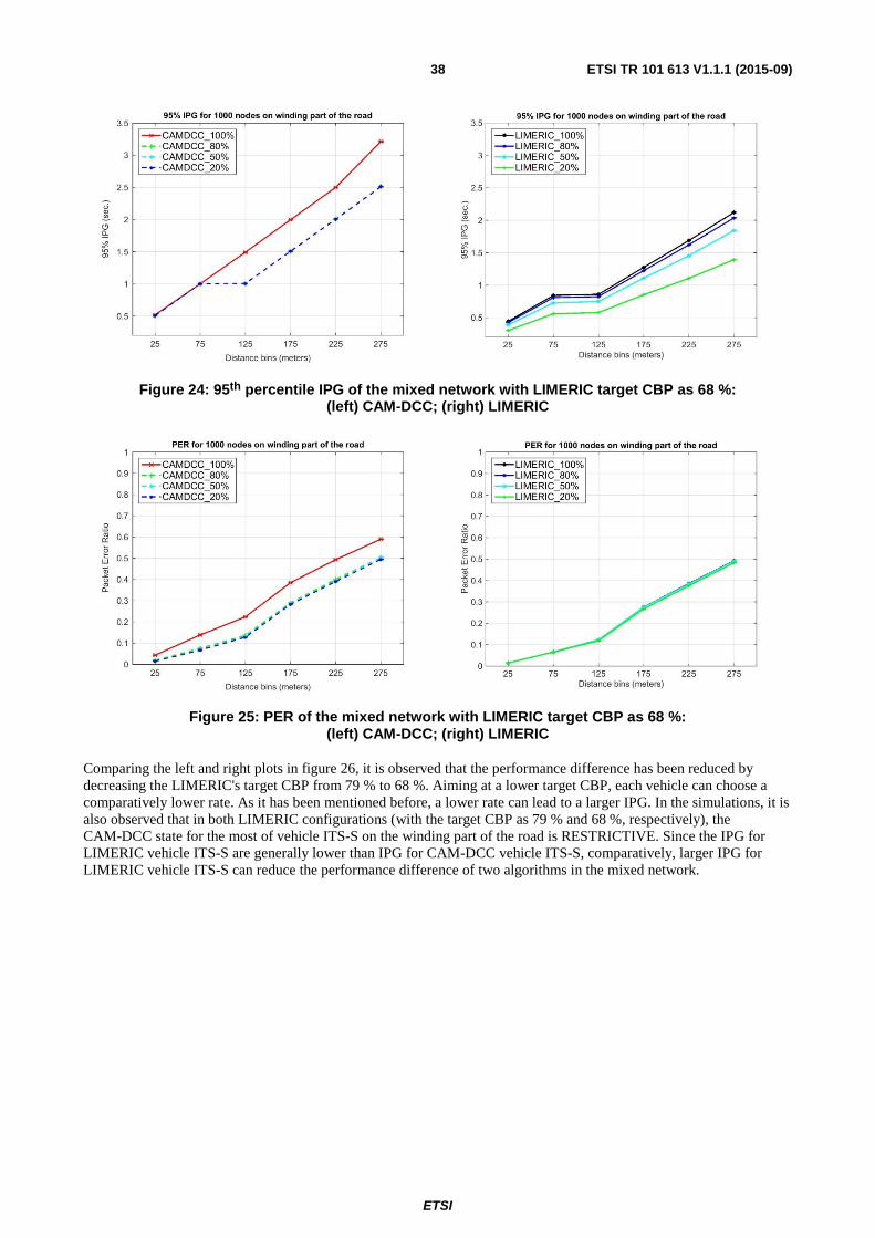
ETSI

ETSI TR 101 613 V1.1.1 (2015-09) 38

Figure 24: 95th percentile IPG of the mixed network with LIMERIC target CBP as 68 %: (left) CAM-DCC; (right) LIMERIC

Figure 25: PER of the mixed network with LIMERIC target CBP as 68 %: (left) CAM-DCC; (right) LIMERIC

Comparing the left and right plots in figure 26, it is observed that the performance difference has been reduced by decreasing the LIMERIC's target CBP from 79 % to 68 %. Aiming at a lower target CBP, each vehicle can choose a comparatively lower rate. As it has been mentioned before, a lower rate can lead to a larger IPG. In the simulations, it is also observed that in both LIMERIC configurations (with the target CBP as 79 % and 68 %, respectively), the CAM-DCC state for the most of vehicle ITS-S on the winding part of the road is RESTRICTIVE. Since the IPG for LIMERIC vehicle ITS-S are generally lower than IPG for CAM-DCC vehicle ITS-S, comparatively, larger IPG for LIMERIC vehicle ITS-S can reduce the performance difference of two algorithms in the mixed network.

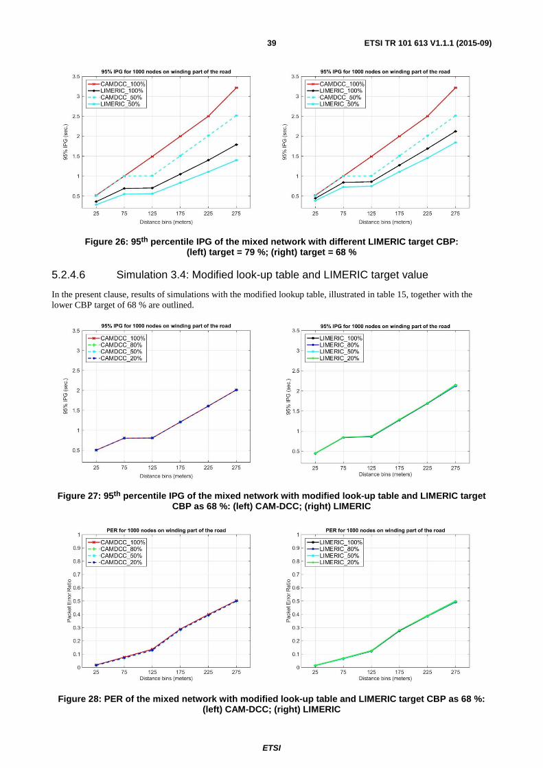
ETSI

ETSI TR 101 613 V1.1.1 (2015-09) 39

Figure 26: 95th percentile IPG of the mixed network with different LIMERIC target CBP: (left) target = 79 %; (right) target = 68 %

5.2.4.6 Simulation 3.4: Modified look-up table and LIMERIC target value

In the present clause, results of simulations with the modified lookup table, illustrated in table 15, together with the lower CBP target of 68 % are outlined.

Figure 27: 95th percentile IPG of the mixed network with modified look-up table and LIMERIC target CBP as 68 %: (left) CAM-DCC; (right) LIMERIC

Figure 28: PER of the mixed network with modified look-up table and LIMERIC target CBP as 68 %: (left) CAM-DCC; (right) LIMERIC

ETSI

ETSI TR 101 613 V1.1.1 (2015-09) 40

Despite of previous observation, combination of these two modifications on CAM-DCC and LIMERIC at the same time could lead to a near-perfect level of fairness in the present scenario. As it has been illustrated in figure 29, the right plot shows these configuration modifications lead to closer performance of CAM-DCC and LIMERIC in terms of 95th percentile IPG.

Figure 29: 95th percentile IPG of the mixed network with different CAM-DCC look-up table and different LIMERIC target:

(left) default look-up table, target = 68 %; (right) modified look-up table, target = 68 %

In addition, as figure 27 depicts, the close performance for this scenario is not related to the portion of the vehicle ITS-S using CAM-DCC to the vehicle ITS-S using LIMERIC. It is particularly important that there is a unique configuration for the number of vehicles in this scenario where fairness is achievable disregarding of ratio of CAM-DCC vehicle ITS-S to LIMERIC vehicle ITS-S. The importance of this set of results is that one of the potential dynamic characteristics of a mixed network for a specific number of vehicles was successfully removed.

Moreover, the performance of CAM-DCC and LIMERIC are also at the same level, in terms of PER, for all the different examined ITS-S ratios. Figure 28 illustrates PER for different LIMERIC and CAM-DCC ITS-S ratios, where CAM-DCC is using the modified look-up table and LIMERIC is using a target CBP equal to 68 %.

Although this result shows that there is a way to provide a fair packet sending opportunity for the two algorithms, varying number of ITS-S can lead to an unbalanced channel usage once again. More investigation is needed to find the impact of number of ITS-S in the mixed network to fairness and performance.

5.3 Future aspects and algorithms

5.3.1 ECPR algorithm

5.3.1.1 Simulator 4: Conclusions

This work proposes ECPR, a combined rate and power DCC algorithm that efficiently achieves the target awareness and rate requirements given by the application context (e.g. target applications, vehicle speed, traffic density) in varying propagation environments. By using path loss exponent estimation, ECPR adapts the TX power level to reach the target awareness range. ECPR controls the channel load by adjusting the rate and TX power level according to the current channel load, range, and rate information. Realistic simulations are performed, incorporating real world information about mobile and static objects (vehicles, buildings, and foliage) and the ECPR is tested in scenarios with varying LOS conditions, highly dynamic network topology, and different environments (highway and urban). The results show that ECPR has the ability to obtain higher rate when the awareness requirements allow it. Compared to a pure message rate control, ECPR is improving the average message rate by 15 %, while keeping the target awareness and channel load within the desired limits. When the awareness requirements are more stringent or the propagation environment is problematic, ECPR efficiently trades rate to improve the awareness by up to 20 percentage points. ECPR can be implemented on top of existing DCC solutions with little effort. Only the transmit power level of the received messages is necessary as an additional information, which can be encoded in the message itself.

ETSI

ETSI TR 101 613 V1.1.1 (2015-09) 41

The following four DCC algorithms were compared:

1) ECPR algorithm [i.20].

2) LIMERIC Algorithm, explained in [i.17], with the following parameters: a = 0,1, b = 1/150.

3) Power-adaptation only algorithm as explained in [i.20], clause III.A.

4) No-DCC scenario (messages are sent at maximum rate and fixed transmit power).

The following conclusions were drawn:

• There is a need for context and environment-based DCC:

- Current and future apps can have different awareness requirements

- Propagation environment strongly affects awareness

• When applied correctly, power control can improve cooperative awareness

• When awareness requirements allow it, the overall system throughput can be increased

• ECPR: practical environment- and context-aware algorithm:

- Adapts to application requirements

- Adapts to propagation environment

- Outperforms LIMERIC rate-only algorithm in terms of cooperative awareness

- Enables higher throughput when awareness allows it


ECPR is an environment and context aware DCC algorithm, which combines power and rate control to improve cooperative awareness by adapting to both specific propagation environments (such as urban intersections, open highways, suburban roads) as well as application requirements (e.g. different target cooperative awareness range). Using the current context that the vehicle operates in (e.g. speed, direction, and application requirement), ECPR adjusts the transmit power level of the messages to reach the desired awareness ratio at the target distance while at the same time controlling the channel load using LIMERIC [i.17], an adaptive rate control algorithm.

The results from this simulation study are twofold:

• Firstly, by performing extensive simulations, including realistic propagation and environment modelling (e.g. transitions between line-of-sight and non-line-of-sight conditions) and realistic vehicle contexts (varying demand on both awareness range and rate), it is shown that ECPR can increase cooperative awareness by more than 20 percentage points compared to a pure message rate control, while keeping the channel load and interference at virtually the same level. When the awareness requirements allow, ECPR can improve the average message rate compared to LIMERIC only.

• Secondly, this study indirectly shows that LIMERIC algorithm has the ability to control the load well in highly dynamic propagation environments.

Detailed explanation of ECPR and further reading is available in [i.20].

5.3.1.3 Simulator 4: Tools and setup

Four DCC approaches are implemented (ECPR, LIMERIC, power-only DCC algorithm, and no DCC scenario) in GEMV2 V2V propagation simulator [i.21], available at http://vehicle2x.net/. GEMV2 is a computationally efficient propagation model for V2V communications, which accounts explicitly for surrounding objects (e.g. buildings, foliage and vehicles).

• Uses outlines of vehicles, buildings, and foliage to distinguish the following three types of links: line of sight (LOS), non-LOS due to vehicles, and non-LOS due to static objects

• Deterministically calculates large-scale signal variations (path-loss and shadowing)

http://vehicle2x.net/

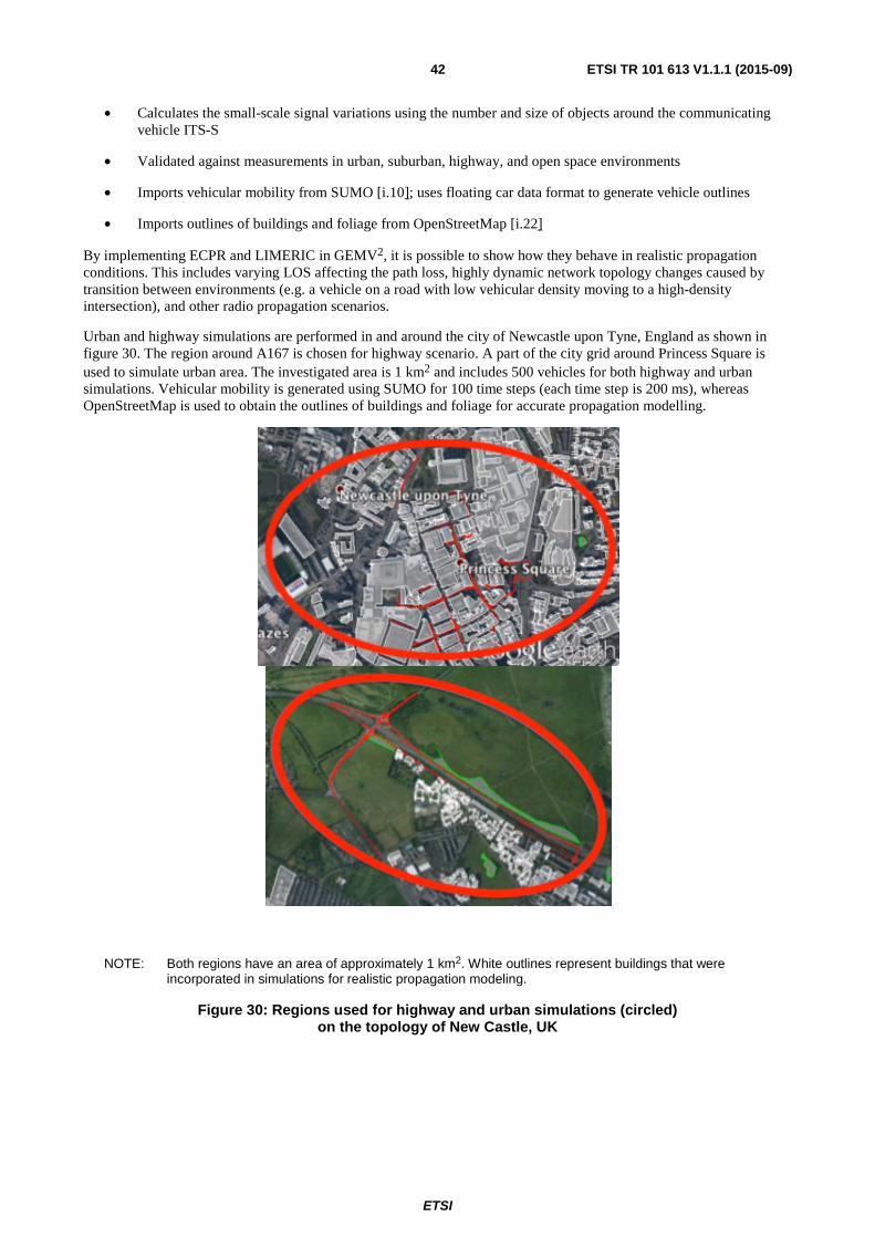
ETSI

ETSI TR 101 613 V1.1.1 (2015-09) 42

• Calculates the small-scale signal variations using the number and size of objects around the communicating vehicle ITS-S

• Validated against measurements in urban, suburban, highway, and open space environments

• Imports vehicular mobility from SUMO [i.10]; uses floating car data format to generate vehicle outlines

• Imports outlines of buildings and foliage from OpenStreetMap [i.22]

By implementing ECPR and LIMERIC in GEMV2, it is possible to show how they behave in realistic propagation conditions. This includes varying LOS affecting the path loss, highly dynamic network topology changes caused by transition between environments (e.g. a vehicle on a road with low vehicular density moving to a high-density intersection), and other radio propagation scenarios.

Urban and highway simulations are performed in and around the city of Newcastle upon Tyne, England as shown in figure 30. The region around A167 is chosen for highway scenario. A part of the city grid around Princess Square is used to simulate urban area. The investigated area is 1 km2 and includes 500 vehicles for both highway and urban simulations. Vehicular mobility is generated using SUMO for 100 time steps (each time step is 200 ms), whereas OpenStreetMap is used to obtain the outlines of buildings and foliage for accurate propagation modelling.

NOTE: Both regions have an area of approximately 1 km2. White outlines represent buildings that were incorporated in simulations for realistic propagation modeling.

Figure 30: Regions used for highway and urban simulations (circled)

on the topology of New Castle, UK

ETSI

ETSI TR 101 613 V1.1.1 (2015-09) 43

To evaluate cooperative awareness in vehicular environments, two metrics are used, as introduced in previous work [i.23]: Neighborhood Awareness Ratio (NAR) and Ratio of Neighbors Above Range (RNAR). These metrics are defined as follows:

• NAR: the proportion of vehicle ITS-S in a specific range from which a message was received in a defined time interval. This metric measures the ability of cooperative message exchange to fulfill its purpose: enable cooperative awareness.

• RNAR: the ratio of neighbors that are above a certain distance from the observed vehicle. This metric gives an indication of potentially unnecessary traffic overheard from distant neighbors (i.e. those that are not relevant for current application context). Once the technology is deployed at a large scale (i.e. with communication equipment installed in most vehicles), such traffic translates to unwanted interference.

In addition to NAR and RNAR, the analysis includes also the performance of DCC in terms of the following metrics.

• Average Message Rate shows the number of messages that a vehicle ITS-S can transmit per second, averaged over all vehicle ITS-S for a given second.

• Average TX Power shows the average TX power level at which a vehicle ITS-S transmits, averaged over all messages for a given second.

• Channel Busy Ratio (CBR) is defined as the proportion of channel time where the energy measured on the channel is above the Clear Channel Assessment (CCA) threshold.

For a given target range r, a target awareness TA equal to 85 %, and omni-directional antennas mounted on the vehicle roof, the DCC performance was evaluated on a single channel. The maximum TX power level was set to 23 dBm and the maximum beacon rate to 10 Hz. Message errors occur due to physical layer effects only (i.e. low signal-to-noise ratio), whereas access layer is assumed to schedule the messages collision-free.

The simulations were done with following DCC algorithms:

1) ECPR algorithm [i.20]. The goal of ECPR is to satisfy the requirements of target awareness levels for different application contexts in different realistic propagation environments, along with utilizing the available channel resources. Due to possibly different application context and environment, the vehicle ITS-S has different target awareness ranges and different target rates. To that end, ECPR uses the TX power level to control awareness range (distance) for the vehicle ITS-S, whereas it uses rate to utilize the channel resources as allowed by the awareness requirements. In other words, ECPR attempts to satisfy the awareness requirements, at the same time maximizing the rate of messages through rate control. In [i.20] it is explained how power and rate control components are implemented, along with the way they are combined to reach the above mentioned goals.

2) LIMERIC Algorithm, explained in [i.17], with the following parameters: α = 0,1, β = 1/150.

3) Power-adaptation only algorithm as explained in [i.20], clause III.A.

4) No-DCC scenario (messages are sent at maximum rate and fixed transmit power).

The simulations are performed for scenarios as described in table 17 according to the algorithm's ability to support each scenario (e.g. LIMERIC cannot support varying awareness ranges, since it is a rate-only algorithm; similarly, power adaptation only cannot support varying message rate).

Table 17: Simulation scenario overview

Scenario Target Awareness Range Target Message Rate Test 1 Same for all vehicles (90 m) Same for all nodes (10 Hz) Test 2 Same for all vehicles (90 m) Uniformly distributed between 5 Hz and 10 Hz Test 3 Chosen randomly from set S = [30, 60, 120, 150, 180] m Same for all nodes (10 Hz) Test 4 Chosen randomly from set S = [30, 60, 120, 150, 180] m Uniformly distributed between 5 Hz and 10 Hz

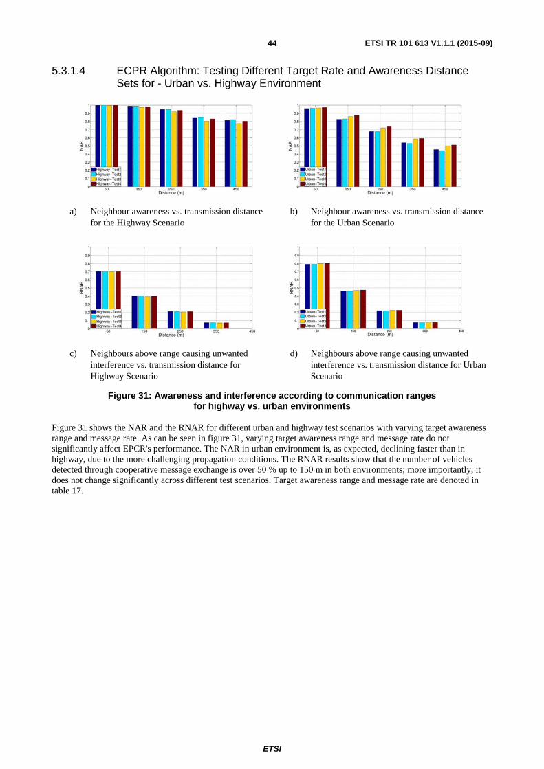
ETSI

ETSI TR 101 613 V1.1.1 (2015-09) 44

5.3.1.4 ECPR Algorithm: Testing Different Target Rate and Awareness Distance Sets for - Urban vs. Highway Environment

a) Neighbour awareness vs. transmission distance for the Highway Scenario

b) Neighbour awareness vs. transmission distance for the Urban Scenario

c) Neighbours above range causing unwanted interference vs. transmission distance for Highway Scenario

d) Neighbours above range causing unwanted interference vs. transmission distance for Urban Scenario

Figure 31: Awareness and interference according to communication ranges for highway vs. urban environments

Figure 31 shows the NAR and the RNAR for different urban and highway test scenarios with varying target awareness range and message rate. As can be seen in figure 31, varying target awareness range and message rate do not significantly affect EPCR's performance. The NAR in urban environment is, as expected, declining faster than in highway, due to the more challenging propagation conditions. The RNAR results show that the number of vehicles detected through cooperative message exchange is over 50 % up to 150 m in both environments; more importantly, it does not change significantly across different test scenarios. Target awareness range and message rate are denoted in table 17.

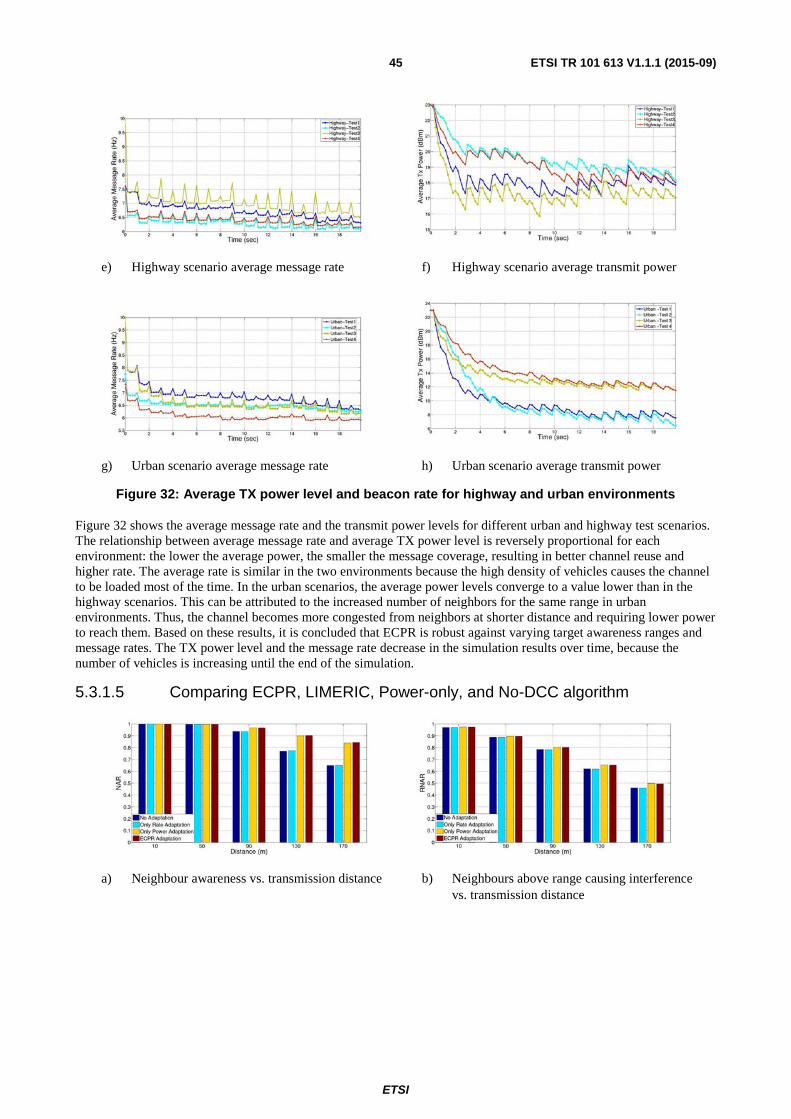
ETSI

ETSI TR 101 613 V1.1.1 (2015-09) 45

e) Highway scenario average message rate f) Highway scenario average transmit power

g) Urban scenario average message rate h) Urban scenario average transmit power

Figure 32: Average TX power level and beacon rate for highway and urban environments

Figure 32 shows the average message rate and the transmit power levels for different urban and highway test scenarios. The relationship between average message rate and average TX power level is reversely proportional for each environment: the lower the average power, the smaller the message coverage, resulting in better channel reuse and higher rate. The average rate is similar in the two environments because the high density of vehicles causes the channel to be loaded most of the time. In the urban scenarios, the average power levels converge to a value lower than in the highway scenarios. This can be attributed to the increased number of neighbors for the same range in urban environments. Thus, the channel becomes more congested from neighbors at shorter distance and requiring lower power to reach them. Based on these results, it is concluded that ECPR is robust against varying target awareness ranges and message rates. The TX power level and the message rate decrease in the simulation results over time, because the number of vehicles is increasing until the end of the simulation.

5.3.1.5 Comparing ECPR, LIMERIC, Power-only, and No-DCC algorithm

a) Neighbour awareness vs. transmission distance b) Neighbours above range causing interference vs. transmission distance

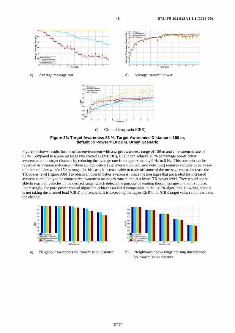
ETSI

ETSI TR 101 613 V1.1.1 (2015-09) 46

c) Average message rate d) Average transmit power

e) Channel busy ratio (CBR)

Figure 33: Target Awareness 85 %, Target Awareness Distance = 150 m, default Tx Power = 10 dBm. Urban Scenario

Figure 33 shows results for the urban environment with a target awareness range of 150 m and an awareness rate of 85 %. Compared to a pure message rate control (LIMERIC), ECPR can achieve 20 % percentage points better awareness at the target distance by reducing the average rate from approximately 9 Hz to 8 Hz. This scenario can be regarded as awareness-focused, where an application (e.g. intersection collision detection) requires vehicles to be aware of other vehicles within 150 m range. In this case, it is reasonable to trade off some of the message rate to increase the TX power level (figure 33(d)) to obtain an overall better awareness. Since the messages that are traded for increased awareness are likely to be cooperative awareness messages transmitted at a lower TX power level. They would not be able to reach all vehicles in the desired range, which defeats the purpose of sending those messages in the first place. Interestingly, the pure power control algorithm achieves an NAR comparable to the ECPR algorithm. However, since it is not taking the channel load (CBR) into account, it is exceeding the upper CBR limit (CBR target value) and overloads the channel.

a) Neighbour awareness vs. transmission distance b) Neighbours above range causing interference vs. transmission distance

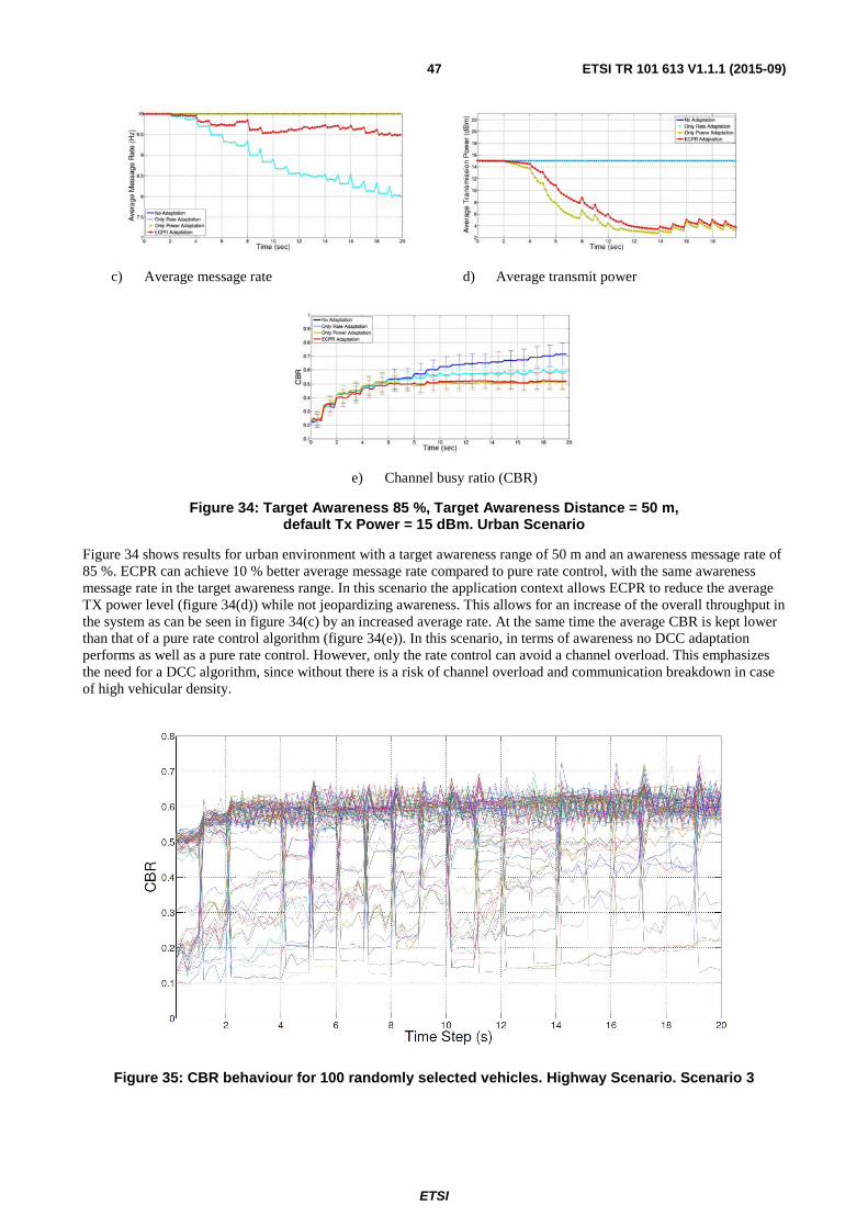
ETSI

ETSI TR 101 613 V1.1.1 (2015-09) 47

c) Average message rate d) Average transmit power

e) Channel busy ratio (CBR)

Figure 34: Target Awareness 85 %, Target Awareness Distance = 50 m, default Tx Power = 15 dBm. Urban Scenario

Figure 34 shows results for urban environment with a target awareness range of 50 m and an awareness message rate of 85 %. ECPR can achieve 10 % better average message rate compared to pure rate control, with the same awareness message rate in the target awareness range. In this scenario the application context allows ECPR to reduce the average TX power level (figure 34(d)) while not jeopardizing awareness. This allows for an increase of the overall throughput in the system as can be seen in figure 34(c) by an increased average rate. At the same time the average CBR is kept lower than that of a pure rate control algorithm (figure 34(e)). In this scenario, in terms of awareness no DCC adaptation performs as well as a pure rate control. However, only the rate control can avoid a channel overload. This emphasizes the need for a DCC algorithm, since without there is a risk of channel overload and communication breakdown in case of high vehicular density.

Figure 35: CBR behaviour for 100 randomly selected vehicles. Highway Scenario. Scenario 3

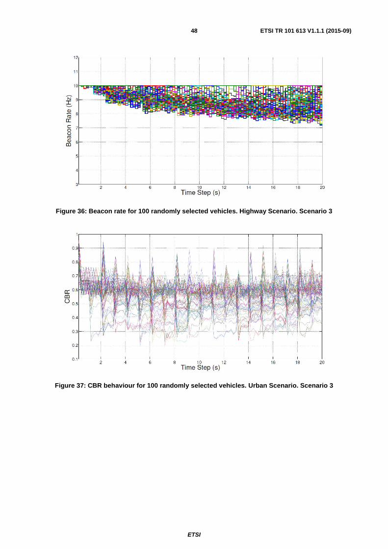
ETSI

ETSI TR 101 613 V1.1.1 (2015-09) 48

Figure 36: Beacon rate for 100 randomly selected vehicles. Highway Scenario. Scenario 3

Figure 37: CBR behaviour for 100 randomly selected vehicles. Urban Scenario. Scenario 3

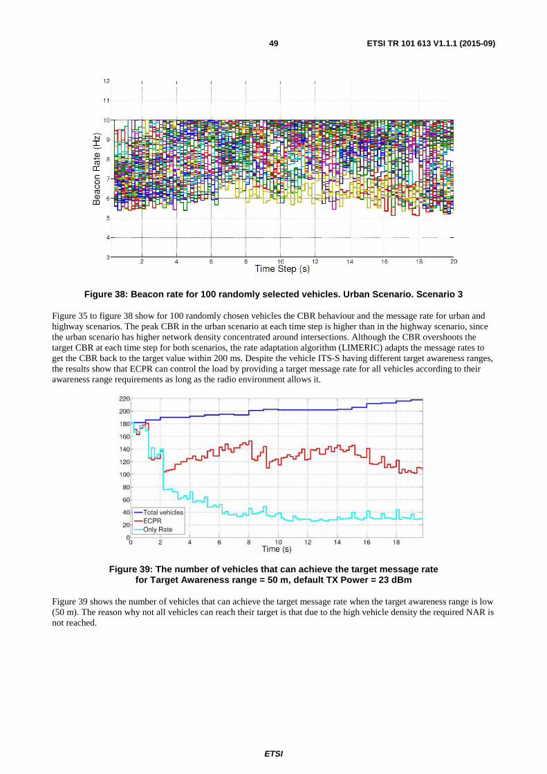
ETSI

ETSI TR 101 613 V1.1.1 (2015-09) 49

Figure 38: Beacon rate for 100 randomly selected vehicles. Urban Scenario. Scenario 3

Figure 35 to figure 38 show for 100 randomly chosen vehicles the CBR behaviour and the message rate for urban and highway scenarios. The peak CBR in the urban scenario at each time step is higher than in the highway scenario, since the urban scenario has higher network density concentrated around intersections. Although the CBR overshoots the target CBR at each time step for both scenarios, the rate adaptation algorithm (LIMERIC) adapts the message rates to get the CBR back to the target value within 200 ms. Despite the vehicle ITS-S having different target awareness ranges, the results show that ECPR can control the load by providing a target message rate for all vehicles according to their awareness range requirements as long as the radio environment allows it.

Figure 39: The number of vehicles that can achieve the target message rate for Target Awareness range = 50 m, default TX Power = 23 dBm

Figure 39 shows the number of vehicles that can achieve the target message rate when the target awareness range is low (50 m). The reason why not all vehicles can reach their target is that due to the high vehicle density the required NAR is not reached.

ETSI

ETSI TR 101 613 V1.1.1 (2015-09) 50

History

Document history

V1.1.1 September 2015 Publication

TR 101 613 - V1.1.1 - Intelligent Transport Systems (ITS ... · Cross Layer DCC Management Entity for operation in the ITS G5A and ... "Intelligent Transport Systems (ITS); Cross

Documents