Toy Model for Tachyon Condensation in Bosonic String Field Theory

arX

iv:h

ep-t

h/01

0707

0v1

9 J

ul 2

001

Preprint typeset in JHEP style. - HYPER VERSION KUL-TF-2001/17

hep-th/0107070

Toy Model for Tachyon Condensation in Bosonic

String Field Theory

Pieter-Jan De Smet and Joris Raeymaekers

Instituut voor theoretische fysica, Katholieke Universiteit Leuven,

Celestijnenlaan 200D, B-3001 Leuven, Belgium.

E-mail: Joris.Raeymaekers, [email protected]

Abstract: We study tachyon condensation in a baby version of Witten’s open string field

theory. For some special values of one of the parameters of the model, we are able to obtain

closed form expressions for the stable vacuum state and for the value of the potential at

the minimum. We study the convergence rate of the level truncation method and compare

our exact results with the numerical results found in the full string field theory.

Keywords: D-branes, Superstring Vacua.

Contents

1. The action 3

2. Cyclicity 4

3. The equation of motion 4

4. Associativity 6

5. Derivation of the star-algebra 7

6. Exact results in case I 8

6.1 Closed form expression for the stable vacuum 8

6.2 Closed form expression for the effective potential 10

6.3 The level truncation method 10

6.4 Convergence properties and comparison to the full string field theory 11

7. Other exact solutions 13

8. Towards the exact solution in case IId? 13

8.1 The star product in momentum space 13

8.2 The equation of motion in momentum space 14

8.3 Numerical results 15

9. Conclusions and topics for further research 15

In this letter, we discuss a simple toy model for tachyon condensation in bosonic

string field theory. The full string field theory problem [1]–[4] consists of extremising a

complicated functional on the Fock space built up from an infinite number of matter and

ghost oscillators. As a first simplification, one can consider the variational problem in the

restricted Hilbert space of states generated by a single matter oscillator. This problem is

still rather nontrivial because the restricted Hilbert space still contains an infinite number

of states. The model we will consider here is precisely of this form and its behaviour closely

resembles the one found in the full theory with level approximation methods. The main

simplification lies in the limited number of degrees of freedom and the fact that we don’t

have to deal with the technicalities of the ghost system.

1

The motivation for considering such simplified models is twofold. First of all, the level

approximation method to the full string theory problem remains largely ‘experimental’:

there doesn’t seem to be a convincing a priori reason why this approximation scheme

converges to the exact answer, nor do we have any information about the rate of convergence

except the ‘experimental’ information we have from considering the first few levels. Our

toy model will allow for the derivation of exact results on the convergence of the level

truncation method albeit in a not fully realistic context.

The second reason for considering toy models is perhaps more fundamental: it would

be of considerable interest to obtain the exact solution for the stable vacuum in the full

theory. Such an exact solution would allow a detailed description of the physics around

the stable vacuum, where interesting phenomena expected to arise [5]. However, despite

many efforts, this solution is lacking at the present time1. The model we will consider is

in some sense the ‘minimal’ problem one should be able to solve if one hopes to find an

analytic solution to the full problem2.

In section 1 we will give the action of the toy model. In its most general form, the

model depends on some parameters that enter in the definition of a star product and are

the analogue of the Neumann coefficients in bosonic string field theory. These parameters

are further constrained if we insist that the toy model star product satisfies some of the

properties that are present in the full string field theory. More specifically, the string field

theory star product satisfies the following properties:

• The three-string interaction term is cyclically symmetric.

• The star product is associative.

• Operators of the form a− a† act as derivations of the star-algebra.

We impose cyclicity of the interaction term in our toy model in section 2. We deduce

the equations of motion in section 3. In section 3 we define the star product for the toy

model. We discuss the restrictions following from imposing associativity of the star product

in section 4. It turns out that we are left with 3 different possibilities, hereafter called case

I, II and III. As is the case for the bosonic string field theory we can also look if there is a

derivation D = a − a† of the star-algebra. This further restricts the cases I, II and III to

case Id, IId and again Id respectively. This is explained in section 5, where we also discuss

the existence of an identity of the star-algebra.

After having set the stage we can start looking for exact solutions. In section 6 we give

the exact results for case I. In particular we are able to write down closed form expressions

for the stable vacuum, the effective potential and its branch structure and the convergence

1See e.g. [6] where a recursive technique was formulated. Other exact solutions are known, see for

example [7].2Other toy models for tachyon condensation were considered in [8, 9, 10].

2

rate of the level truncation method. We also compare these results with the behaviour

found in bosonic string field theory. In section 7 we mention the other exact solutions we

have found. In section 8, we discuss the case IId which perhaps bears the most resemblance

to the full string field theory problem. In this case, it is possible to recast the equation

of motion in the form of an ordinary second order nonlinear differential equation. This

equation is not of the Painleve type and we have not been able to find an exact solution.

Here too, it is possible to get very accurate information about the stable vacuum using

the level truncation method. We conclude in section 9 with some suggestions for further

research.

1. The action

The toy model we consider has the following action (the potential energy is equal to minus

the action):

S(ψ) = −1

2〈ψ|(L0 − 1)|ψ〉 − 1

3〈V ||ψ〉|ψ〉|ψ〉 (1.1)

where L0 is the usual kinetic operator L0 = a†a and [a, a†] = 1. Let us denote the Fock

space which is built up in the usual way by H. The “string field” |ψ〉 is simply a state in

this Fock space H and can thus be expanded as

|ψ〉 = ψ0|0〉 + ψ1a†|0〉 + ψ2(a

†)2|0〉 + · · · ,

where the coefficients ψ0, ψ1, · · · are complex numbers. To illustrate the analogy between

this toy model and Witten’s bosonic string field theory [11], the complex numbers ψi in

the toy model correspond to the space-time fields in the bosonic string field theory in the

Siegel gauge. The term −1 in the kinetic part of the action should be thought of as the

zero point energy in the bosonic string. In this way, the state |0〉 has negative energy.

The interaction term is defined as follows:

〈V ||ψ〉|ψ〉|ψ〉 = 123〈0| exp(1

2

3∑

i,j=1

Nijaiaj) |ψ〉1|ψ〉2|ψ〉3. (1.2)

The numbers Nij mimic the Neumann coefficient in Witten’s string field theory [12]. There

they carry additional indices Nij,kl ηµν where k, l = 1, . . . ,∞ label the different modes of

the string and µ, ν = 1, . . . , 26 are space-time indices.

We have introduced three copies of the Fock space H. The extra subscript on a state

denotes the copy the state is in:

if |ψ〉 =∑

m

ψma†m|0〉 ∈ H,

then |ψ〉i =∑

m

ψma†mi |0〉i ∈ Hi for i = 1, 2, 3.

3

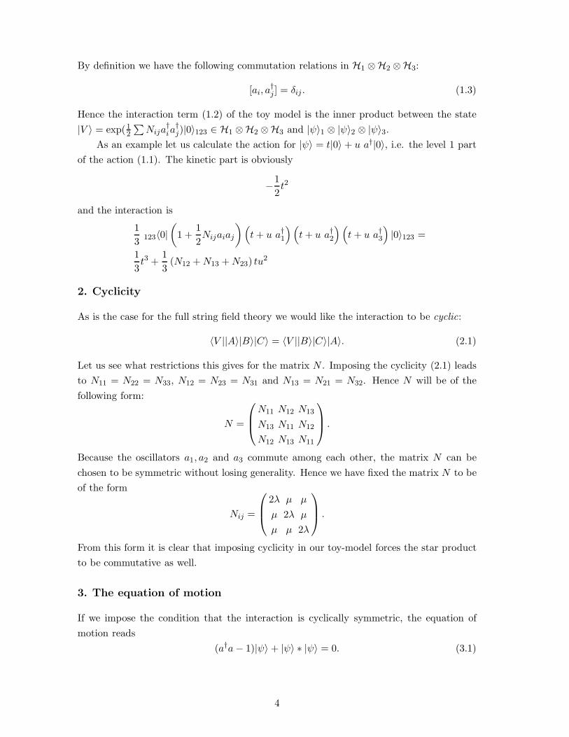
By definition we have the following commutation relations in H1 ⊗H2 ⊗H3:

[ai, a†j ] = δij . (1.3)

Hence the interaction term (1.2) of the toy model is the inner product between the state

|V 〉 = exp(12

∑

Nija†ia

†j)|0〉123 ∈ H1 ⊗H2 ⊗H3 and |ψ〉1 ⊗ |ψ〉2 ⊗ |ψ〉3.

As an example let us calculate the action for |ψ〉 = t|0〉 + u a†|0〉, i.e. the level 1 part

of the action (1.1). The kinetic part is obviously

−1

2t2

and the interaction is

1

3123〈0|

(

1 +1

2Nijaiaj

)

(

t+ u a†1

)(

t+ u a†2

)(

t+ u a†3

)

|0〉123 =

1

3t3 +

1

3(N12 +N13 +N23) tu

2

2. Cyclicity

As is the case for the full string field theory we would like the interaction to be cyclic:

〈V ||A〉|B〉|C〉 = 〈V ||B〉|C〉|A〉. (2.1)

Let us see what restrictions this gives for the matrix N . Imposing the cyclicity (2.1) leads

to N11 = N22 = N33, N12 = N23 = N31 and N13 = N21 = N32. Hence N will be of the

following form:

N =

N11 N12 N13

N13 N11 N12

N12 N13 N11

.

Because the oscillators a1, a2 and a3 commute among each other, the matrix N can be

chosen to be symmetric without losing generality. Hence we have fixed the matrix N to be

of the form

Nij =

2λ µ µ

µ 2λ µ

µ µ 2λ

.

From this form it is clear that imposing cyclicity in our toy-model forces the star product

to be commutative as well.

3. The equation of motion

If we impose the condition that the interaction is cyclically symmetric, the equation of

motion reads

(a†a− 1)|ψ〉 + |ψ〉 ∗ |ψ〉 = 0. (3.1)

4

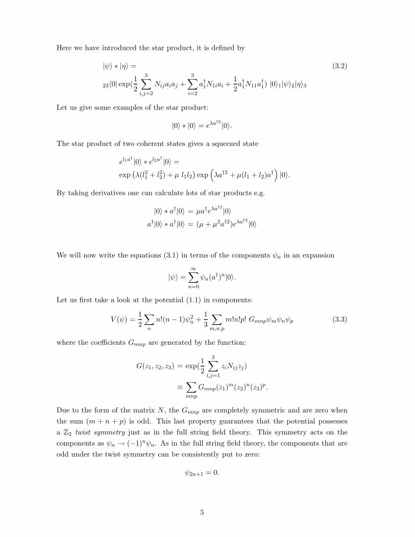
Here we have introduced the star product, it is defined by

|ψ〉 ∗ |η〉 = (3.2)

23〈0| exp(1

2

3∑

i,j=2

Nijaiaj +3∑

i=2

a†1N1iai +1

2a†1N11a

†1) |0〉1|ψ〉2|η〉3

Let us give some examples of the star product:

|0〉 ∗ |0〉 = eλa†2 |0〉.

The star product of two coherent states gives a squeezed state

el1a† |0〉 ∗ el2a† |0〉 =

exp(

λ(l21 + l22) + µ l1l2)

exp(

λa†2 + µ(l1 + l2)a†)

|0〉.

By taking derivatives one can calculate lots of star products e.g.

|0〉 ∗ a†|0〉 = µa†eλa†2 |0〉a†|0〉 ∗ a†|0〉 = (µ+ µ2a†2)eλa†2 |0〉

We will now write the equations (3.1) in terms of the components ψn in an expansion

|ψ〉 =

∞∑

n=0

ψn(a†)n|0〉.

Let us first take a look at the potential (1.1) in components:

V (ψ) =1

2

∑

n

n!(n− 1)ψ2n +

1

3

∑

m,n,p

m!n!p! Gmnpψmψnψp (3.3)

where the coefficients Gmnp are generated by the function:

G(z1, z2, z3) = exp(1

2

3∑

i,j=1

ziNijzj)

≡∑

mnp

Gmnp(z1)m(z2)

n(z3)p.

Due to the form of the matrix N , the Gmnp are completely symmetric and are zero when

the sum (m + n + p) is odd. This last property guarantees that the potential possesses

a Z2 twist symmetry just as in the full string field theory. This symmetry acts on the

components as ψn → (−1)nψn. As in the full string field theory, the components that are

odd under the twist symmetry can be consistently put to zero:

ψ2n+1 = 0.

5

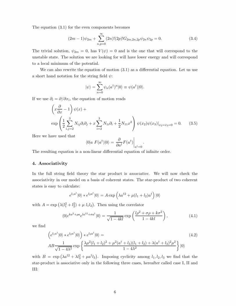
The equation (3.1) for the even components becomes

(2m− 1)ψ2m +∞∑

n,p=0

(2n)!(2p)!G2m,2n,2pψ2nψ2p = 0. (3.4)

The trivial solution, ψ2m = 0, has V (ψ) = 0 and is the one that will correspond to the

unstable state. The solution we are looking for will have lower energy and will correspond

to a local minimum of the potential.

We can also rewrite the equation of motion (3.1) as a differential equation. Let us use

a short hand notation for the string field ψ:

|ψ〉 =∞∑

n=0

ψn(a†)n|0〉 ≡ ψ(a†)|0〉.

If we use ∂i = ∂/∂xi, the equation of motion reads(

x∂

∂x− 1

)

ψ(x) +

exp

1

2

3∑

i,j=2

Nij∂i∂j + x3∑

i=2

N1i∂i +1

2N11x

2

ψ(x2)ψ(x3)|x2=x3=0 = 0. (3.5)

Here we have used that

〈0|a F (a†)|0〉 =∂

∂a†F (a†)

∣

∣

∣

∣

a†=0

.

The resulting equation is a non-linear differential equation of infinite order.

4. Associativity

In the full string field theory the star product is associative. We will now check the

associativity in our model on a basis of coherent states. The star-product of two coherent

states is easy to calculate:

el1a† |0〉 ∗ el2a† |0〉 = A exp(

λa†2 + µ(l1 + l2)a†)

|0〉

with A = exp(

λ(l21 + l22) + µ l1l2)

. Then using the correlator

〈0|eka2+ρaela†2+σa† |0〉 =

1√1 − 4kl

exp

(

lρ2 + σρ+ kσ2

1 − 4kl

)

, (4.1)

we find(

el1a† |0〉 ∗ el2a† |0〉)

∗ el3a† |0〉 = (4.2)

AB1√

1 − 4λ2exp

{

λµ2(l1 + l2)2 + µ2(a† + l3)(l1 + l2) + λ(a† + l3)

2µ2

1 − 4λ2

}

|0〉

with B = exp(

λa†2 + λl23 + µa†l3)

. Imposing cyclicity among l1, l2, l3 we find that the

star-product is associative only in the following three cases, hereafter called case I, II and

III:

6

I. µ = 0, then N =

2λ 0 0

0 2λ 0

0 0 2λ

II. 2λ = µ− 1, then N =

µ− 1 µ µ

µ µ− 1 µ

µ µ µ− 1

III. λ = 1/2, then N =

1 µ µ

µ 1 µ

µ µ 1

However, due to the factor 1/√

1 − 4λ2 in equation (4.2) the star product of 3 coherent

states diverges in the last case. Therefore we should look for another proof of associativity

in this case. We will not do this, we just discard this case.

5. Derivation of the star-algebra

Let us now look if D = a− a† is a derivation of the ∗-algebra:

D(A ∗B) = DA ∗B +A ∗DB where A and B are two string fields.

This is analogous to αµ1 − αµ

−1 being a derivation in the full string field theory, see for

example [13]. It is easy to see that for D to be a derivation we need∑

i

(ai − a†i )|V 〉 = 0. (5.1)

Let us calculate the left hand side of (5.1):

∑

i

(ai − a†i )|V 〉 =∑

i

(∂

∂a†i− a†i )|V 〉

=∑

i

(Nija†j − a†i )|V 〉

This is zero if and only if ( 1 1 1 ) · (N − 1) = 0.

• case I

We need 3(2λ− 1) = 0 so λ = 1/2. Hence D is a derivation if and only if N = 1. We

will call this trivial case henceforth case Id.

• case II

We need 2µ+ µ− 2 = 0, hence µ = 2/3. In this case we have

N =

−1/3 2/3 2/3

2/3 −1/3 2/3

2/3 2/3 −1/3

(5.2)

Henceforth, we call this subcase IId.

7

• case III

We need 2µ = 0 so µ = 0. This reduces to case Id.

For the case Id we will show in section 6 that there is no non-perturbative vacuum.

Therefore we consider the value (5.2) as the most important special case that we would

like to solve exactly in our toy-model.

In the full string field theory, an important role is played by the identity string field I

i.e. a string field obeying I ∗ A = A = A ∗ I for (almost) all string fields A3. In the toy

model, there exists an identity string field I only in case II. In this case we have for the

identity I

|I〉 =

√2µ− 1

µexp

(

1 − µ

4µ− 2a†2)

|0〉.

Using the correlator (4.1), the reader can easily check that

|I〉 ∗ ela† |0〉 = ela† |0〉

for all coherent states ela† |0〉, thus proving that I is the identity. Proving that there is no

identity if N does not belong to case II is most easily done by first arguing that the identity

should be a Gaussian in the creation operator a† and then showing that one can not find

a Gaussian which acts as the identity on all coherent states. In case IId the identity string

field reduces to

|I〉 =2√3

exp

(

1

2a†2)

|0〉 (5.3)

6. Exact results in case I

6.1 Closed form expression for the stable vacuum

We now construct the exact solution in the case I, where

N =

2λ 0 0

0 2λ 0

0 0 2λ

.

The coefficients G2m,2n,2p entering in the equation of motion (3.4) are particularly simple

in this case:

G2m,2n,2p =λm+n+p

m!n!p!.

Equation (3.4) reduces to

ψ2m =λm

(1 − 2m)m!g(λ)2 (6.1)

3There are some anomalies in the ghost sector, I is not an identity of the star algebra on all states,

see [13].

8

where we have defined a function g(λ) by

g(λ) =

∞∑

n=0

(2n)!λn

n!ψ2n(λ).

Multiplying equation (6.1) by (2m)!λm/m! and summing over m we obtain g(λ):

g(λ) =

(

∑

n

λ2n(2n)!

(n!)2(1 − 2n)

)−1

=1√

1 − 4λ2

Hence our candidate for the stable vacuum |vac〉 is

|vac〉 =1

1 − 4λ2

∞∑

n=0

λn

n!(1 − 2n)(a†)2n|0〉

Using the representation (3.5), it is also possible to derive a generating function for

the coefficients ψ2n. Putting λ = −l2, the differential equation (3.5) reduces to

(

x∂

∂x− 1

)

ψ(x) + exp−l2(

∂22 + ∂2

3 + x2)

ψ(x2)ψ(x3)∣

∣

x2=x3=0= 0

This is(

x∂

∂x− 1

)

ψ(x) + e−l2x2

c2 = 0,

where c is just a number

c = e−l2∂2xψ(x)

∣

∣

∣

x=0.

A solution of this differential equation is

ψ(x) =1

1 − 4l4φ(lx),

where φ(x) is the function

φ(x) = exp(−x2) +√πx erf(x)

= −+∞∑

m=0

(−x2)m

m! (2m− 1).

The energy difference between the false and true vacuum can be expressed entirely in

terms of the function g(λ):

V (vac) = −1

6g(λ)3 = −1

6(1 − 4λ2)−3/2.

It is clear that the true vacuum only exists for |λ| < 12 since the value of the potential

becomes imaginary outside this range. Also, for |λ| > 12 , the state |vac〉 is no longer

normalisable. Note that for the special case Id, λ = 12 , there does not seem to be a true

vacuum.

9

6.2 Closed form expression for the effective potential

We can also determine the exact effective tachyon potential V (t) by solving for the ψ2n, n > 0

in terms of t ≡ ψ0. The equation for these components becomes:

ψ2m(λ, t) =λm

(1 − 2m)m!(t+ h(λ, t))2 for m > 0 (6.2)

where we have defined

h(λ, t) =∞∑

n=1

(2n)!λn

n!ψ2n(λ, t).

Multiplying equation (6.2) by (2m)!λm/m! and summing over m we get a quadratic equa-

tion for h(λ, t):

h(λ, t) = (√

1 − 4λ2 − 1)(t+ h(λ, t))2.

The two solutions h±

h± =1

2(1 −√

1 − 4λ2)

(

−2t(1 −√

1 − 4λ2) − 1 ±√

4t(1 −√

1 − 4λ2) + 1

)

will give rise to two branches of the effective potential. When we also impose the equation

for t, we see that the unstable vacuum t = 0 and the stable vacuum t = 11−4λ2 lie on

the same branch (i.e. the one determined by h+) just as in the full string field theory.

Substituting h± in (6.2) to obtain the coefficients ψ2n±(λ, t) and substituting those in (3.3)

we find the exact form of the two branches of the effective potential V±(t):

V± = −1

2t2 +

h2±

2(1 −√

1 − 4λ2)+

1

3(t+ h±)3.

As is the case in the full bosonic string field theory, the branch V+(t), which links the

unstable and the stable vacuum, terminates at a finite negative value t∗, given in this case

by

t∗ = − 1

4(1 −√

1 − 4λ2). (6.3)

At this point, the two branches meet. It is also the only point where they intersect, since

V− > V+ for all other values of t.

6.3 The level truncation method

We can also discuss the convergence of the level truncation method in this case. We will

focus on the level (2k, 6k) approximation to the tachyon potential. This means that we

include the fields up to level 2k and keep all the terms in the potential involving these

fields. In this approximation, the equation for the extremum is just (3.4) with all sums

now running from 0 to k. The solution proceeds just as in the previous section. First one

solves for the function g(k)(λ):

g(k)(λ) ≡(

k∑

n=0

λ2n(2n)!

(n!)2(1 − 2n)

)−1

=(√

1 − 4λ2 + E(λ, k))−1

.

10

The function E(λ, k), which represents the error we make by truncating at level 2k, can

be expressed in terms of special functions

E(λ, k) =21+2kλ2(1+k)Γ(1

2 + k) 2F1(1,12 + k, 2 + k; 4λ2)√

π(k + 1)!.

The level-truncated expressions for the components of the approximate vacuum state

|vac(k)〉 and the value of V(2k,6k) at the minimum are given by:

ψ(k)2m =

λm

(1 − 2m)m!g(k)(λ)2

V(2k,6k)(vac(k)) = −1

6g(k)(λ)3

The determination of the level-truncated effective tachyon potential also proceeds as

before. The result is

V(2k,6k)±(t) = −1

2t2 +

h(k)±

2

2(1 −√

1 − 4λ2 − E(λ, k))+

1

3(t+ h

(k)± )3

with

h(k)± =

1

2(1 −√

1 − 4λ2 − E(λ, k))

(

− 2t(1 −√

1 − 4λ2 − E(λ, k)) − 1

±√

4t(1 −√

1 − 4λ2 −E(λ, k)) + 1)

.

Again, the potential has two branches which intersect at a finite negative value t(k)∗ :

t(k)∗ = − 1

4(1 −√

1 − 4λ2 − E(λ, k))(6.4)

A plot of both branches of the potential for k = 0, 1, 2 at λ = 0.4, as compared to the

exact result, is shown in figure 1.

6.4 Convergence properties and comparison to the full string field theory

The results of the previous sections allow us to derive some exact results concerning the

convergence properties of the level truncation method in this model and to compare them

with the behaviour found in the full string field theory using numerical methods [4]. For

this purpose, we need the asymptotic behaviour of the function E(λ, k) for large level k

[17]:

E(λ, k) ∼ 2λ2

√π(1 − 4λ2)

k−3/2(4λ2)k[1 + O(k−1)] for k → ∞. (6.5)

Hence the error we make in the level approximation to the coefficients of the true vacuum

and the value of the potential at its minimum goes like

ψ2m − ψ(k)2m ∼ 22k+2λ2k+m+2k−3/2

√πm!(1 − 2m)(1 − 4λ2)5/2

V (vac) − V(2k,6k)(vac(k)) ∼ −λ

2k−3/2(4λ2)k√π(1 − 4λ2)3

11

0 1 2 3 4 5

-1

-0.5

0

0.5

1

1.5

V (t)

t

(0, 0)(2, 6)(4, 12)(6, 18)exact

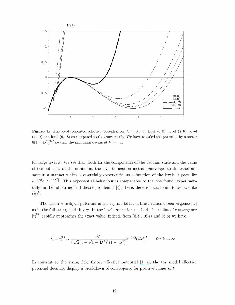
Figure 1: The level-truncated effective potential for λ = 0.4 at level (0, 0), level (2, 6), level

(4, 12) and level (6, 18) as compared to the exact result. We have rescaled the potential by a factor

6(1 − 4λ2)3/2 so that the minimum occurs at V = −1.

for large level k. We see that, both for the components of the vacuum state and the value

of the potential at the minimum, the level truncation method converges to the exact an-

swer in a manner which is essentially exponential as a function of the level: it goes like

k−3/2e−k| ln 4λ2|. This exponential behaviour is comparable to the one found ‘experimen-

tally’ in the full string field theory problem in [4]: there, the error was found to behave like

(13 )k.

The effective tachyon potential in the toy model has a finite radius of convergence |t∗|as in the full string field theory. In the level truncation method, the radius of convergence

|t(k)∗ | rapidly approaches the exact value; indeed, from (6.3), (6.4) and (6.5) we have

t∗ − t(k)∗ ∼ λ2

8√π(1 −

√1 − 4λ2)2(1 − 4λ2)

k−3/2(4λ2)k for k → ∞.

In contrast to the string field theory effective potential [1, 4], the toy model effective

potential does not display a breakdown of convergence for positive values of t.

12

7. Other exact solutions

We can also find the exact minimum in case II when µ = 1, i.e. when

N =

0 1 1

1 0 1

1 1 0

.

We need to solve the following equation:

(

x∂

∂x− 1

)

ψ(x) + exp (∂2∂3 + x(∂2 + ∂3))ψ(x2)ψ(x3)|x2=x3=0 = 0.

A solution of this equation is ψ(x) = 1.

|false vac〉 = 0|0〉 |true vac〉 = 1|0〉

More generally we can also solve

N =

0 µ µ

µ 0 µ

µ µ 0

,

for general µ, again the solution is ψ(x) = 1. However this case is not associative if µ 6= 1.

8. Towards the exact solution in case IId?

8.1 The star product in momentum space

In section 4 we have deduced that D = a − a† is a derivation of the star algebra. If we

write the creation and annihilation operators in terms of the momentum and coordinate

operators:{

a† = 1√2

(p + ix),

a = 1√2

(p − ix),

we see that D is proportional to ∂/∂p. Therefore it is tempting to anticipate that the star

product will reduce to an ordinary product in momentum space, and this is indeed the

case4. If we write the states in momentum representation:

|ψ〉 =

∫

dp ψ(p)|p〉p,

4In Witten’s string field theory the operators Dµn = α

µn + (−1)n

αµ−n are derivations of the star algebra.

This suggests going to the k – space for the odd matter oscillators αµ2n+1 and to the x – space for the even

matter oscillators αµ2n. See [14] where an analysis along these lines was performed. In Witten’s string field

theory the star product reduces to a matrix product in the split string formalism [15].

13

where the states |p〉p are the eigenstates of the momentum operator p, normalized in such a

way that 〈p1|p2〉 = δ(p1 − p2) — we use the extra subscript to denote which representation

we are using. We find

|ψ〉 ∗ |η〉 =

∫

dp π1/4

√

3

2ψ(p)η(p)|p〉p (8.1)

and

〈V ||ψ1〉|ψ2〉|ψ3〉 = π1/4

√

3

2

∫

dp ψ1(p)ψ2(p)ψ3(p). (8.2)

This last equation is easy to prove on a basis of coherent states. If |ψi〉 = exp (lia†)|0〉,

then

〈V ||ψ1〉|ψ2〉|ψ3〉 = e lT Nl.

Let us verify if we get the same result in momentum space. A coherent state is given by a

Gaussian in momentum space:

ela† |0〉a =

1

π1/4exp(−1

2l2 +

√2 l k − k2

2).

Equation (8.2) then holds by Gaussian integration.

As a check on our result we will verify that the state |I〉 given by (5.3) is the identity

in momentum space. In momentum space we have

|I〉 =

√

2

3

1

π1/41 as a function in momentum space,

therefore we have for arbitrary states ψ

|I〉 ∗ |ψ〉 =

√

2

3

1

π1/41 · π1/4

√

3

2ψ(k) = ψ(k),

as it should be.

8.2 The equation of motion in momentum space

The equation of motion we want to solve now becomes in momentum space

(a†a− 1)|ψ〉 + |ψ〉 ∗ |ψ〉

=1

2

(

− ∂2

∂p2+ (p2 − 3)

)

ψ + π1/4

√

3

2ψ(p)2 = 0.

If we drop some constants, the differential equation we are left with reads

∂2

∂p2ψ(p) = (p2 − 3)ψ(p) + ψ(p)2. (8.3)

So we see that instead of the infinite order differential equation we started with, we have

now a second order non-linear differential equation. A large body of literature exists (see

14

e.g. [19]) on second order differential equations that have the Painleve property, meaning

that the solutions to these equations have no movable critical points. Such equations

can be transformed to one of 50 equations whose solutions can be expressed in terms of

known transcendental functions. Applying the algorithm described in [20], one finds that

equation (8.3) is not of the Painleve type due to the presence of movable logarithmic

singularities. Hence we have been unsuccesful in solving (8.3).

8.3 Numerical results

Even though we are not able to find a closed form solution in this case, we can get good

approximate results with the level truncation method. We give the potential including

fields up to level 4. It reads:

V (|ψ〉) =−ψ0

2

2+ψ0

3

3− ψ0

2 ψ2

3+ ψ2

2 + ψ0 ψ22 +

13ψ23

27+ψ0

2 ψ4

3

−34ψ0 ψ2 ψ4

9+

41ψ22 ψ4

27+ 36ψ4

2 +227ψ0 ψ4

2

27+

319ψ2 ψ42

27+

1249ψ43

81

We can minimize this action and we find

at level 0: |ψ〉 = 1.|0〉with V (ψ) = −0.166667.

at level 2: |ψ〉 = (1.05083 + 0.0870701 a†2)|0〉with V (ψ) = −0.181514

at level 4: |ψ〉 = (1.0508 + 0.0867394 a†2 − 0.000383389 a†4)|0〉with V (ψ) = −0.181521

at level 6: |ψ〉 = (1.05082 + 0.0867768 a†2 − 0.000408059 a†4 − 0.0000352206 a†6)|0〉with V (ψ) = −0.181523

at level 8: |ψ〉 = (1.05082 + 0.0867771 a†2 − 0.000412528 a†4 − 0.0000341415 a†6

+1.788 · 10−6 a†8)|0〉with V (ψ) = −0.181524

at level 10: |ψ〉 = (1.05082 + 0.0867771 a†2 − 0.000412537 a†4 − 0.0000339848 a†6

+1.76475 · 10−6a†8 − 4.54233 · 10−8a†10)|0〉with V (ψ) = −0.181524

We see that the level truncation method clearly converges to some definite answer.

9. Conclusions and topics for further research

We simplified Witten’s open string field theory by dropping all the ghosts and keeping

only one matter oscillator. The model we constructed closely resembles the full string field

theory on the following points:

15

• There is a false vacuum and a stable vacuum.

• The interaction is given in terms of “Neumann coefficients” and can be written by

using an associative star product.

• There is a notion of level truncation which converges rapidly to the correct answer.

For some special values of one of the parameters of the model, we were able to obtain the

exact solution for the stable vacuum state and the value of the potential at the minimum.

For other values of the parameters we did not succeed in constructing the exact mini-

mum of the tachyon potential. This does not mean that it is impossible to solve Witten’s

string field theory exactly. In the full string field theory there is a lot more symmetry

around: for example Witten’s string field theory has a huge gauge invariance and one

could try to solve the equation of motion by making a pure – gauge like ansatz [16].

Therefore maybe a natural thing to do is to set up a toy model that includes some of the

ghost oscillators in such a way that there is also a gauge invariance. Another research topic

would be to set up a toy model of Berkovits’ superstring field theory (see [18] for a recent

review). It also should not be too difficult to try to mathematically prove the convergence

of the level truncation method in these toy models. This might teach us something about

why the level truncation method converges in the full string field theory.

Acknowledgments

This work was supported in part by the European Commission RTN project HPRN-CT-

2000-00131. The authors would like to thank Walter Troost for discussions and especially

Martin Schnabl for collaboration on several parts of this work. P.J.D.S. is aspirant FWO-

Vlaanderen.

References

[1] V. A. Kostelecky and S. Samuel, “On A Nonperturbative Vacuum For The Open Bosonic

String,” Nucl. Phys. B 336, 263 (1990).

[2] V. A. Kostelecky and R. Potting, “Expectation Values, Lorentz Invariance, and CPT in the

Open Bosonic String,” Phys. Lett. B 381, 89 (1996) [hep-th/9605088].

[3] A. Sen and B. Zwiebach, “Tachyon condensation in string field theory,” JHEP 0003, 002

(2000) [hep-th/9912249].

[4] N. Moeller and W. Taylor, “Level truncation and the tachyon in open bosonic string field

theory,” Nucl. Phys. B 583, 105 (2000) [hep-th/0002237].

[5] A. Sen, “Fundamental strings in open string theory at the tachyonic vacuum,” hep-th/0010240;

I. Ellwood and W. Taylor, “Open string field theory without open strings,” hep-th/0103085;

M. Kleban, A. E. Lawrence and S. Shenker, “Closed strings from nothing,” hep-th/0012081;

16

L. Rastelli, A. Sen and B. Zwiebach, “String field theory around the tachyon vacuum,” hep-

th/0012251.

[6] V. A. Kostelecky and R. Potting, “Analytical construction of a nonperturbative vacuum for

the open bosonic string,” Phys. Rev. D 63, 046007 (2001) [hep-th/0008252].

[7] T. Takahashi and S. Tanimoto, “Wilson Lines and Classical Solutions in Cubic Open String

Field Theory,” hep-th/0107046

[8] J. A. Minahan and B. Zwiebach, “Field theory models for tachyon and gauge field string dy-

namics,” JHEP 0009 (2000) 029 [hep-th/0008231]. “Effective tachyon dynamics in superstring

theory,” JHEP 0103 (2001) 038 [hep-th/0009246]. “Gauge fields and fermions in tachyon ef-

fective field theories,” JHEP 0102 (2001) 034 [hep-th/0011226].

[9] D. Ghoshal and A. Sen, “Tachyon condensation and brane descent relations in p-adic string

theory,” Nucl. Phys. B 584 (2000) 300 [hep-th/0003278].

J. A. Minahan, “Mode interactions of the tachyon condensate in p-adic string theory,” JHEP

0103 (2001) 028 [hep-th/0102071].

J. A. Minahan, “Quantum corrections in p-adic string theory,” hep-th/0105312.

[10] D. J. Gross and V. Periwal, “String field theory, noncommutative Chern-Simons theory and

Lie algebra cohomology,” hep-th/0106242.

[11] E. Witten, “Noncommutative Geometry And String Field Theory,” Nucl. Phys. B 268, 253

(1986).

[12] D. J. Gross and A. Jevicki, “Operator Formulation Of Interacting String Field Theory,” Nucl.

Phys. B 283 (1987) 1. “Operator Formulation Of Interacting String Field Theory. 2,” Nucl.

Phys. B 287 (1987) 225.

[13] L. Rastelli and B. Zwiebach, “Tachyon potentials, star products and universality,” hep-

th/0006240.

[14] I. Bars, “Map of Witten’s * to Moyal’s *,” hep-th/0106157.

[15] D. J. Gross and W. Taylor, “Split string field theory. I, II” hep-th/0105059, hep-th/0106036.

[16] M. Schnabl, “String field theory at large B-field and noncommutative geometry,” JHEP 0011

(2000) 031 [hep-th/0010034].

[17] M. Abramowitz and I. Stegun (1970), “Handbook of Mathematical Functions,” Dover Publi-

cations, Inc., New York.

[18] N. Berkovits, “Review of open superstring field theory,” hep-th/0105230.

[19] E. Kamke, “Differentialgleichungen: Losungsmethoden und Losungen. 1: Gewohnliche Differ-

entialgleichungen”, Teubner Stuttgart, 1983.

[20] M.J. Ablowitz, A. Ramani, H. Segur, “A connection between nonlinear evolution equations

and ordinary differential equations of P-type.1.”, J. Math. Phys. 21, 715 (1980).

17