Towards the experimental clarification of quarkonium polarization

CER

N-P

H-E

P-20

10-0

2213

/06/

2010

EUROPEAN LABORATORY FOR PARTICLE PHYSICS

Towards the experimental clarification

of quarkonium polarization

Pietro Faccioli1), Carlos Lourenco2), Joao Seixas1,3) and Hermine K. Wohri1)

Abstract

We highlight issues which are often underestimated in the experimental analyses onquarkonium polarization: the relation between the parameters of the angular distri-butions and the angular momentum composition of the quarkonium, the importanceof the choice of the reference frame, the interplay between observed decay and produc-tion kinematics, and the consequent influence of the experimental acceptance on thecomparison between experimental measurements and theoretical calculations. Giventhe puzzles raised by the available experimental results, new measurements must pro-vide more detailed information, such that physical conclusions can be derived withoutrelying on model-dependent assumptions. We describe a frame-invariant formalismwhich minimizes the dependence of the measurements on the experimental accep-tance, facilitates the comparison with theoretical calculations, and probes systematiceffects due to experimental biases. This formalism is a direct and generic consequenceof the rotational invariance of the dilepton decay distribution and is independent ofany assumptions specific to particular models of quarkonium production. The useof this improved approach, which exploits the intrinsic multidimensionality of theproblem, will significantly contribute to a faster progress in our understanding ofquarkonium production, especially if adopted as a common analysis framework bythe LHC experiments, which will soon perform analyses of quarkonium polarizationin proton-proton collisions.

Submitted to Euro. Phys. J. C

1) Laboratorio de Instrumentacao e Fısica Experimental de Partıculas (LIP),Lisbon, Portugal

2) CERN, Geneva, Switzerland3) Physics Department, Instituto Superior Tecnico (IST), Lisbon, Portugal

1 Introduction

Detailed studies of quarkonium prodution should provide significant progress in ourunderstanding of quantum chromodynamics (QCD) [1]. However, our present under-standing of this physics topic is rather limited, despite the multitude of experimentaldata accumulated over more than 30 years. The pT differential J/ψ and ψ′ directproduction cross sections measured (in the mid 1990’s) by CDF, in pp collisions at1.8 TeV [2], were seen to be around 50 times larger than the available expectations,based on leading order calculations made in the scope of the Colour Singlet Model.The non-relativistic QCD (NRQCD) framework [3], where quarkonia can also be pro-duced as coloured quark pairs, succeeded in describing the measurements, opening anew chapter in the studies of quarkonium production physics. However, these calcu-lations depend on non-perturbative parameters, the long distance colour octet matrixelements, which have been freely adjusted to the data, thereby decreasing the impactof the resulting agreement between data and calculations. More recently, calcula-tions of next-to-leading-order (NLO) QCD corrections to colour-singlet quarkoniumproduction showed an important increase of the high-pT rate, significantly decreasingthe colour-octet component needed to reproduce the quarkonium production crosssections measured at the Tevatron [4].

Given this situation, differential cross sections are clearly insufficient informationto ensure further progress in our understanding of quarkonium production. Experi-mental studies of the polarization of the JPC = 1−− quarkonium states, which decayinto lepton pairs, will certainly provide very useful complementary information. Infact, the competing mechanisms dominating in the different theoretical approacheslead to very different expected polarizations of the produced quarkonia. On one hand,the NRQCD calculations [5, 6, 7], dominated by the colour-octet component, predictthat, at Tevatron or LHC energies and at asymptotically high pT, the directly pro-duced ψ′ and J/ψ mesons are produced almost fully transversely polarized (i.e. withdominant angular momentum component Jz = ±1) with respect to their own mo-mentum direction (the helicity frame). On the other hand, according to the new NLOcalculations of colour-singlet quarkonium production [4] these states should show astrong longitudinal (Jz = 0) polarization component.

Having two very different theoretical predictions appears to be an ideal situationwhen seen from an experimentalist’s perspective, as one may think that it should berelatively straightforward to discriminate between the two theory frameworks usingexperimental measurements. Somewhat surprisingly, however, this is not the case. Infact, the present experimental knowledge is incomplete and contradictory. Studies ofthe ψ′ polarization have been published on the basis of data collected by the CDF IIexperiment [8]. Unfortunately, the large experimental uncertainties caused by thesmall size of the data samples prevent from drawing meaningful conclusions. Inprinciple, a more precise test of the theoretical predictions should be provided by theJ/ψ data, given their much higher statistical accuracy. However, the experimentalperspective is more complicated in this case, because a significant fraction (aroundone third [9]) of promptly produced J/ψ mesons (i.e. excluding contributions from

2

B hadron decays) comes from χc and ψ′ feed-down decays. This sizeable source ofindirectly produced J/ψ mesons is not subtracted from the current measurements,and its kinematic dependence is not precisely known. Despite this limitation, it seemssafe to say that the pattern measured by CDF [8] of a slightly longitudinal polarizationof the inclusive prompt J/ψ’s is incompatible with any of the two theory approachesmentioned above. The situation is further complicated by the intriguing lack ofcontinuity between fixed-target and collider results, which can only be interpreted inthe framework of some specific (and speculative) assumptions still to be tested [10].

The bb system should satisfy the non-relativistic approximation much better thanthe cc case. For this reason, the Υ data are expected to represent the most decisive testof NRQCD. However, the comparison with the existing Υ(1S) polarization data fromTevatron [11, 12] is far from conclusive. The results indicate that, for pT < 15 GeV/c,the Υ(1S) is produced either unpolarized (CDF) or longitudinally polarized (D0) inthe helicity frame, and this discrepancy cannot be reasonably attributed to the differ-ent rapidity windows covered by the two experiments. Furthermore, the precision ofthe data for pT higher than 15 GeV/c is not sufficient to provide a significant test ofthe crucial hypothesis that very high-pT quarkonia, produced by the fragmentation ofan outgoing (almost on-shell) gluon, are fully transversely polarized along their owndirection. At lower energy and pT, the E866 experiment [13] has shown yet a differentpolarization pattern: the Υ(2S) and Υ(3S) states have maximal transverse polariza-tion, with no significant dependence on transverse or longitudinal momentum, withrespect to the direction of motion of the colliding hadrons (Collins-Soper frame). Un-expectedly, the Υ(1S), whose spin and angular momentum properties are identicalto the ones of the heavier Υ states, is, instead, found to be only weakly polarized.These results give interesting physical indications. First, the maximal polarization ofΥ(2S) and Υ(3S) along the direction of the interacting particles places strong con-straints on the topology and spin properties of the underlying elementary productionprocess. Second, the small Υ(1S) polarization suggests that the bottomonium familymay have a peculiar feed-down hierarchy, with a very significant fraction of the lowermass state being produced indirectly; at the same time, the polarization of the Υ’scoming from χb decays should be substantially different from the polarization of thedirectly produced ones.

This rather confusing situation demands a significant improvement in the accu-racy and detail of the polarization measurements, ideally distinguishing between theproperties of directly and indirectly produced states. We remind that the lack of aconsistent description of the polarization properties represents today’s biggest uncer-tainty in the simulation of the LHC quarkonium production measurements and willprobably be the largest contribution to the systematic error affecting the measure-ments of quarkonium production cross sections and kinematic distributions. Indeed,the probability that the detector accepts lepton pairs resulting from decays of quarko-nium states is strongly dependent on the polarization of those states. Therefore, evenfrom a purely experimental point of view it is very unsatisfactory that essential prop-erties of these objects, such as kinematic details of how they decay into lepton pairs

3

(on which their reconstruction is based), are subjected to such a high degree of un-certainty.

It is true that measurements of the quarkonium decay angular distributions arechallenging, multi-dimensional kinematic problems, which require large event samplesand a very high level of accuracy in the subtraction of spurious kinematic correlationsinduced by the detector acceptance. The complexity of the experimental problemswhich have to be faced in the polarization measurements is testified, for example,by the disagreement between the CDF results obtained in Run I and Run II forthe J/ψ [14, 8] and by the contradictory results obtained by CDF and D0 for theΥ(1S). However, it is also true, as we shall emphasize in this paper, that most exper-iments have exploited, and presented in the published reports, only a fraction of thephysical information derivable from the data. This happens, for example, when themeasurement is performed in only one polarization frame and is limited to the polarprojection of the decay angular distribution. As we have already argued in Ref. [10],these incomplete measurements do not allow definite physical conclusions. At best,they confine such conclusions to a genuinely model-dependent framework. Moreover,such a fragmentary description of the observed physical process obviously reduces thechances of detecting possible biases induced by not fully controlled systematic effects.

In this paper we review the mathematical framework for the description of theobservable polarization of quarkonium states decaying electromagnetically into leptonpairs. We focus our attention on aspects that need to be taken in consideration in theanalysis of the data, so as to maximize the physical significance of the measurementand provide all elements for its unambiguous interpretation within any theoreticalframework. By increasing the level of detail of the physical information extractedfrom the data, the proposed methodologies also offer the possibility of performingconsistency checks which can expose unaccounted detector or analysis biases. Theonly relevant theoretical ingredients of our discussion are the quantum properties ofangular momentum and basic conservation rules of the electromagnetic interaction(parity, fermion chirality). All the results presented here are, therefore, valid ingeneral for any quarkonium production mechanism.

In Section 2 we define the concept of polarization and give simple examples ofhow basic production mechanisms can lead to the formation of polarized quarkoniumstates. We then focus on the dilepton decay distribution of 3S1 quarkonia, a rela-tively simple case, and provide detailed geometric and kinematic considerations. InSection 3 we recall the basic principles leading to the general expression describingthe angular distribution of the decay products, while in Section 4 we describe howthe observed anisotropy parameters depend on the choice of the reference frame.Section 5 is devoted to a detailed description of how the production kinematics in-fluences the observed polarization, depending on the quarkonium momentum and onthe observation frame. We also discuss quantitatively the influence of the intrinsicparton transverse momenta on the polarization measurement when the natural axisis along the relative flight direction of the colliding partons. In Section 6 we derivethe existence of a frame-independent identity which relates the observable parameters

4

of the decay distribution to one frame-invariant polarization parameter. We discusshow this relation, formally including the Lam-Tung identity [15] as a particular case,improves the representation of polarization results and can be used to perform consis-tency checks in the experimental analyses. We continue with some remarks, given inSection 7, on how the existence of intrinsic parton transverse momentum affects thepolarization measurement. We conclude, in Section 8, with a few examples inspiredfrom existing experimental measurements, which should provide concrete evidencefor the usefulness of the approaches discussed in this paper, in view of ensuring animproved understanding of quarkonium production.

2 Basic polarization concepts

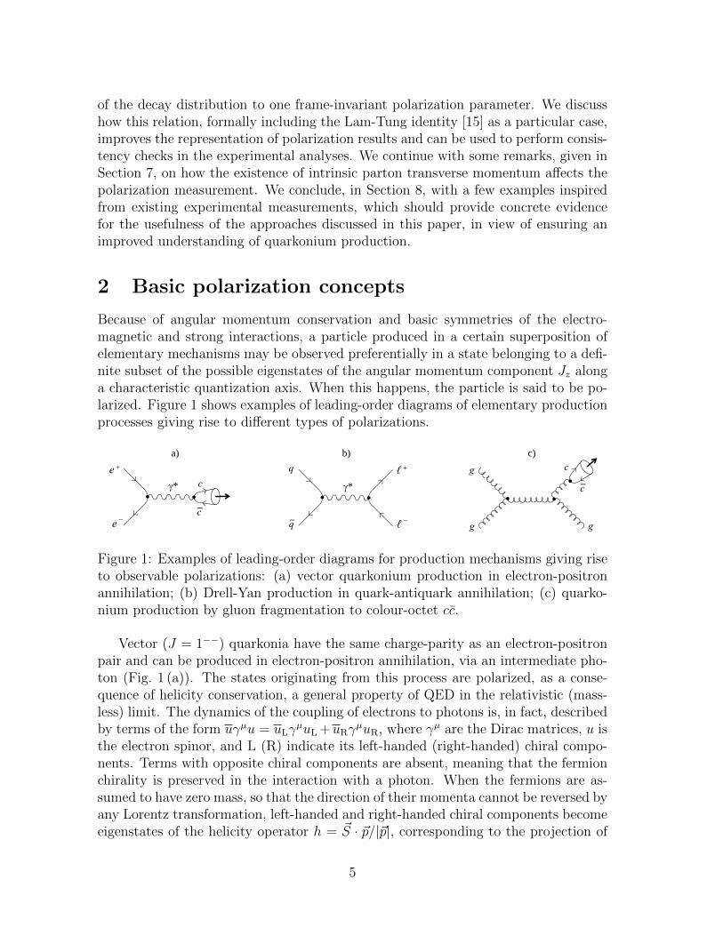
Because of angular momentum conservation and basic symmetries of the electro-magnetic and strong interactions, a particle produced in a certain superposition ofelementary mechanisms may be observed preferentially in a state belonging to a defi-nite subset of the possible eigenstates of the angular momentum component Jz alonga characteristic quantization axis. When this happens, the particle is said to be po-larized. Figure 1 shows examples of leading-order diagrams of elementary productionprocesses giving rise to different types of polarizations.

qe +

b)a)

γ* γ* c

qe −c

cgℓ +

c)

c

g gℓ −

Figure 1: Examples of leading-order diagrams for production mechanisms giving riseto observable polarizations: (a) vector quarkonium production in electron-positronannihilation; (b) Drell-Yan production in quark-antiquark annihilation; (c) quarko-nium production by gluon fragmentation to colour-octet cc.

Vector (J = 1−−) quarkonia have the same charge-parity as an electron-positronpair and can be produced in electron-positron annihilation, via an intermediate pho-ton (Fig. 1 (a)). The states originating from this process are polarized, as a conse-quence of helicity conservation, a general property of QED in the relativistic (mass-less) limit. The dynamics of the coupling of electrons to photons is, in fact, describedby terms of the form uγµu = uLγ

µuL +uRγµuR, where γµ are the Dirac matrices, u is

the electron spinor, and L (R) indicate its left-handed (right-handed) chiral compo-nents. Terms with opposite chiral components are absent, meaning that the fermionchirality is preserved in the interaction with a photon. When the fermions are as-sumed to have zero mass, so that the direction of their momenta cannot be reversed byany Lorentz transformation, left-handed and right-handed chiral components becomeeigenstates of the helicity operator h = ~S · ~p/|~p|, corresponding to the projection of

5

the spin on the momentum direction. In this case, chirality conservation becomes he-licity conservation. In the diagram of Fig. 1 (a), this rule implies that the annihilatingelectron and positron must have opposite helicities, because the intermediate photonhas zero (fermion) helicity. Since in the laboratory their momenta are opposite, theirspins must be parallel. Because of angular momentum conservation, the producedquarkonium has, thus, angular momentum component Jz = ±1 along the directionof the colliding leptons. This precise QED prediction (the relative amplitude for theJz = 0 component is of order me/Ee ' 3×10−4 for J/ψ production and smaller for Υproduction) is commonly used as a base assumption in quarkonium measurements inelectron-positron annihilations (as, for example, in the recent analysis of Ref. [16]).The fact that the dilepton system coupled to a photon is a pure Jz = ±1 state is alsoan essential ingredient in the determination of the expression for the dilepton-decayangular distributions of vector quarkonia (see Section 3).

The same reasoning can be applied to the production of Drell-Yan lepton pairsin quark-antiquark annihilation (Fig. 1 (b)): the quark and antiquark, in the limitof vanishing masses, must annihilate with opposite helicities, resulting in a dileptonstate having Jz = ±1 along the direction of their relative velocity. The experimentalverification of this basic mechanism has reached an impressive level of accuracy [13].Quark helicity is conserved also in QCD, when the masses can be neglected. Similarlyto the Drell-Yan case, quarkonia originating from quark-antiquark annihilation (intointermediate gluons) will thus tend, provided they are produced alone, to have theirangular momentum vectors “aligned” (Jz = ±1) along the beam direction. Thisprediction is in good agreement with the χc1, χc2 and ψ′ polarizations measured inlow-energy proton-antiproton collisions [17, 18].

At very high pT, quarkonium production at hadron colliders should mainly pro-ceed by gluon fragmentation [19]. In NRQCD, heavy-quark velocity scaling rulesfor the non perturbative matrix elements, combined with the αS and 1/pT powercounting rules for the parton cross sections, predict that J/ψ and ψ′ production

at high pT is dominated by gluon fragmentation into the color-octet state cc[3S(8)1 ]

(Fig. 1 (c)). Transitions of the gluon to other allowed colour and angular momentumconfigurations, containing the cc in either a colour-singlet or a colour-octet state,with spin S = 0, 1 and angular momentum L = 0, 1, 2, . . ., as well as additionalgluons (cc[1S

(8)0 ]g, cc[3P

(8)J ]g, cc[3S

(1)1 ]gg, etc.), are more and more suppressed with

increasing pT. Up to small corrections, the fragmenting gluon is believed to be onshell and have, therefore, helicity ±1. This property is inherited by the cc[3S

(8)1 ]

state and remains intact during the non-perturbative transition to the colour-neutralphysical state, via soft-gluon emission. In this model, the observed charmonium has,thus, angular momentum component Jz = ±1, this time not along the direction ofthe beam, but along its own flight direction.

“Unpolarized” quarkonium has the same probability, 1/(2J + 1), to be found ineach of the angular momentum eigenstates, Jz = −J,−J + 1, . . . ,+J . This is thecase, for example, in the colour evaporation model [20]. In this framework, similarlyto NRQCD, the QQ pair is produced at short distances in any colour and angular

6

momentum configuration. However, contrary to NRQCD, no hierarchy constraintsare imposed on these configurations, so that the cross section turns out to be domi-nated by QQ pairs with vanishing angular momentum (1S0), in either colour-singletor colour-octet states. In their long distance evolution through soft gluon emissions,J = 0 states get their colour randomized, assuming the correct quantum numbers ofthe physical quarkonium. As a result, the final angular momentum vector ~J has nopreferred alignment.

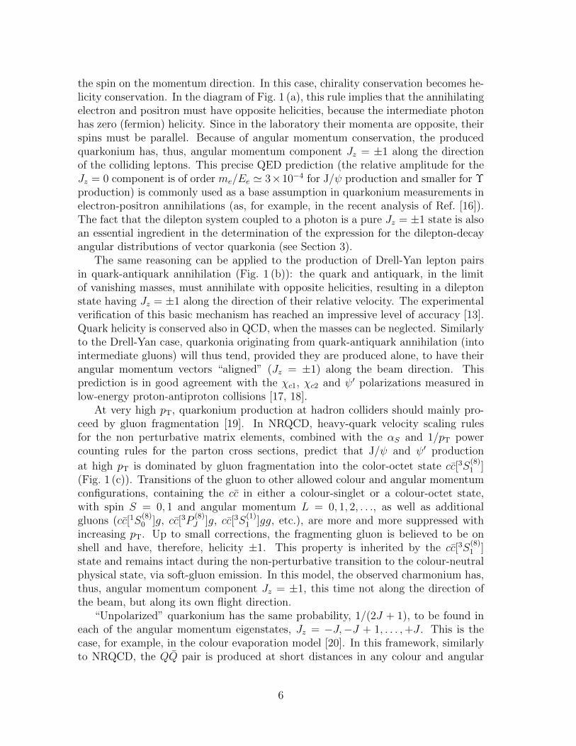
In two-body decays (such as the 3S1 → `+`− case considered in this paper), thegeometrical shape of the angular distribution of the two decay products (emitted back-to-back in the quarkonium rest frame) reflects the polarization of the quarkoniumstate. A spherically symmetric distribution would mean that the quarkonium wouldbe, on average, unpolarized. Anisotropic distributions signal polarized production.

quarkonium

rest frame

production

plane

yx

z

ϑ

φ

ℓ +

Figure 2: The coordinate system for the measurement of a two-body decay angulardistribution in the quarkonium rest frame. The y axis is perpendicular to the planecontaining the momenta of the colliding beams. The polarization axis z is chosenaccording to one of the possible conventions described in Fig. 3.

The measurement of the distribution requires the choice of a coordinate system,with respect to which the momentum of one of the two decay products is expressedin spherical coordinates. In inclusive quarkonium measurements, the axes of thecoordinate system are fixed with respect to the physical reference provided by thedirections of the two colliding beams as seen from the quarkonium rest frame. Figure 2illustrates the definitions of the polar angle ϑ, determined by the direction of one of thetwo decay products (e.g. the positive lepton) with respect to the chosen polar axis, andof the azimuthal angle ϕ, measured with respect to the plane containing the momentaof the colliding beams (“production plane”). The actual definition of the decayreference frame with respect to the beam directions is not unique. Measurementsof the quarkonium decay distributions have used three different conventions for the

7

production plane y

zHX zGJ

b1 b2

zCS

b1 b2

Q collisioncentre

of massframe

b1 b2

quarkoniumrest

frame

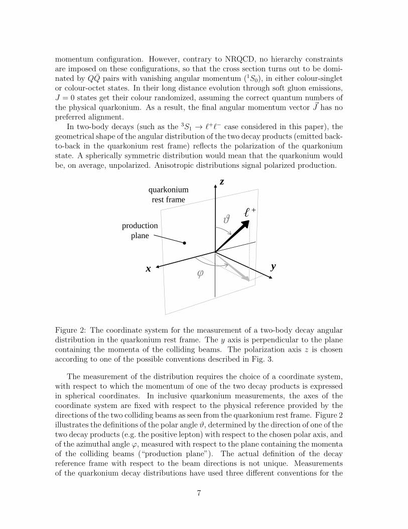
Figure 3: Illustration of three different definitions of the polarization axis z (CS:Collins-Soper, GJ: Gottfried-Jackson, HX: helicity) with respect to the directions ofmotion of the colliding beams (b1, b2) and of the quarkonium (Q).

orientation of the polar axis (see Fig. 3): the direction of the momentum of one of thetwo colliding beams (Gottfried-Jackson frame [21], GJ), the opposite of the directionof motion of the interaction point (i.e. the flight direction of the quarkonium itselfin the center-of-mass of the colliding beams: helicity frame, HX) and the bisectorof the angle between one beam and the opposite of the other beam (Collins-Soperframe [22], CS). The motivation of this latter definition is that, in hadronic collisions,it coincides with the direction of the relative motion of the colliding partons, whentheir transverse momenta are neglected (the validity and limits of this approximationare discussed in detail in Section 7). For our considerations, we will take the HXand CS frames as two extreme (physically relevant) cases, given that the GJ polaraxis represents an intermediate situation. We note that these two frames differ by arotation of 90◦ around the y axis when the quarkonium is produced at high pT andnegligible longitudinal momentum (pT � |pL|). All definitions become coincident inthe limit of zero quarkonium pT. In this limit, moreover, for symmetry reasons anyazimuthal dependence of the decay distribution is physically forbidden.

We conclude this section by defining the somewhat misleading nomenclature whichis commonly used (and adopted, for convenience, also in this paper) for the polar-ization of vector mesons. These particles share the quantum numbers of the photonand are therefore said, by analogy with the photon, to be “transversely” polarizedwhen they have spin projection Jz = ±1. The counterintuitive adjective originallyrefers to the fact that the electromagnetic field carried by the photon oscillates inthe transverse plane with respect to the photon momentum, while the photon spin isaligned along the momentum. “Longitudinal” polarization means Jz = 0. By furtherextension, the same terms are also used to describe the “spin alignment” of vectorquarkonia not only with respect to their own momenta (HX frame), but also withrespect to any other chosen reference direction (such as the GJ or CS axes).

8

3 Dilepton decay angular distribution

Vector quarkonia, such as the J/ψ, ψ′ and Υ(nS) states, can decay electromagneti-cally into two leptons. The reconstruction of this channel represents the cleanest way,both from the experimental and theoretical perspectives, of measuring their produc-tion yields and polarizations. In this and the following sections we discuss how todetermine experimentally the “spin alignment” of a vector quarkonium by measuringthe dilepton decay angular distribution. For convenience we mention explicitly theJ/ψ as the decaying particle, but considerations and results are valid for any J = 1−−

state.We begin by studying the case of a single production “subprocess”, here defined

as a process where the J/ψ is formed as a given superposition of the three J = 1eigenstates, Jz = +1,−1, 0 with respect to the polarization axis z:

|V 〉 = b+1 |+1〉+ b−1 |−1〉+ b0 |0〉 . (1)

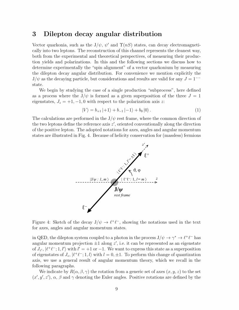
The calculations are performed in the J/ψ rest frame, where the common direction ofthe two leptons define the reference axis z′, oriented conventionally along the directionof the positive lepton. The adopted notations for axes, angles and angular momentumstates are illustrated in Fig. 4. Because of helicity conservation for (massless) fermions

z'

ϑ, φ

ℓ+

z|J/ψ : 1, m ⟩

ϑ, φ

J/ψrest frame

| ℓ+ℓ−: 1, l = m ⟩

f

ℓ−

Figure 4: Sketch of the decay J/ψ → `+`−, showing the notations used in the textfor axes, angles and angular momentum states.

in QED, the dilepton system coupled to a photon in the process J/ψ → γ∗ → `+`− hasangular momentum projection ±1 along z′, i.e. it can be represented as an eigenstateof Jz′ , |`+`−; 1, l′〉 with l′ = +1 or−1. We want to express this state as a superpositionof eigenstates of Jz, |`+`−; 1, l〉 with l = 0,±1. To perform this change of quantizationaxis, we use a general result of angular momentum theory, which we recall in thefollowing paragraphs.

We indicate by R(α, β, γ) the rotation from a generic set of axes (x, y, z) to the set(x′, y′, z′), α, β and γ denoting the Euler angles. Positive rotations are defined by the

9

right-hand rule. An eigenstate |J,M ′〉 of Jz′ can then be expressed as a superpositionof the eigenstates |J,M〉 of Jz through the rotation transformation [23]

|J,M ′〉 =+J∑

M=−J

DJMM ′(R) |J,M〉 . (2)

The (complex) rotation matrix elements DJMM ′ are defined as

DJMM ′(α, β, γ) = e−iMαdJMM ′(β)e−iM′γ (3)

in terms of the (real) reduced matrix elements

dJMM ′(β) =

min(J+M,J−M ′)∑t=max(0,M−M ′)

(−1)t

×√

(J +M)! (J −M)! (J +M ′)! (J −M ′)!

(J +M − t)! (J −M ′ − t)! t! (t−M +M ′)!(4)

×(

cosβ

2

)2J+M−M ′−2t(sin

β

2

)2t−M+M ′

.

The rotation we need in our case has the effect of bringing one quantization axis (z)to coincide with another (z′). The most general rotation performing this projectioncan be parametrized with β = ϑ and α = −γ = ϕ. The dilepton angular momentumstate is therefore expressed in terms of eigenstates of Jz as

|`+`−; 1, l′〉 =∑l=0,±1

D1l l′(ϕ, ϑ,−ϕ) |`+`−; 1, l〉 . (5)

The amplitude of the partial process J/ψ(m)→ `+`−(l′) represented in Fig. 4 is

Bml′ =∑l=0,±1

D1∗ll′ (ϕ, ϑ,−ϕ) 〈`+`−; 1, l | B | J/ψ; 1,m〉

= B D1∗ml′(ϕ, ϑ,−ϕ) , (6)

where we imposed that the transition operator B is of the form〈`+`−; 1, l | B | J/ψ; 1,m〉 = B δml because of angular momentum conservation,with B independent of m (for rotational invariance). The total amplitude forJ/ψ → `+`−(l′), where the J/ψ is given by the superposition written in Eq. 1, is

Bl′ =∑

m=−1,+1

bmB D1∗ml′(ϕ, ϑ,−ϕ)

=∑

m=−1,+1

am D1∗ml′(ϕ, ϑ,−ϕ) . (7)

10

The probability of the transition is obtained by squaring Eq. 7 and summing over the(unobserved) spin alignments (l′ = ±1) of the dilepton system, with equal weightsattributed, for parity conservation, to the two configurations. Using Eq. 3, withd10,±1 = ± sinϑ/

√2, d1±1,±1 = (1 + cosϑ)/2 and d1±1,∓1 = (1 − cosϑ)/2 (from Eq. 3),

one obtains the angular distribution

W (cosϑ, ϕ) ∝∑l′=±1

|Bl′ |2 ∝N

(3 + λϑ)(1 + λϑ cos2 ϑ

+ λϕ sin2 ϑ cos 2ϕ + λϑϕ sin 2ϑ cosϕ (8)

+ λ⊥ϕ sin2 ϑ sin 2ϕ + λ⊥ϑϕ sin 2ϑ sinϕ) ,

with N = |a0|2 + |a+1|2 + |a−1|2 and

λϑ =N − 3|a0|2

N + |a0|2,

λϕ =2 Re[a

(i)∗+1 a−1]

N + |a0|2,

λϑϕ =

√2 Re[a

(i)∗0 (a+1 − a−1)]N + |a0|2

, (9)

λ⊥ϕ =2 Im[a∗+1a−1]

N + |a0|2,

λ⊥ϑϕ =−√

2 Im[a∗0(a+1 + a−1)]

N + |a0|2.

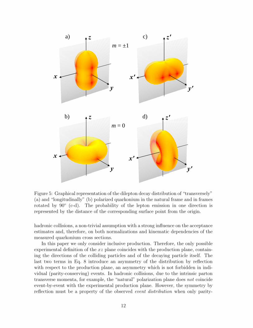
Figure 5 shows the shapes of the dilepton decay distributions in the two polarizationcases m = ±1 (a) and m = 0 (b); the m = +1 and m = −1 configurations are indis-tinguishable because of rotation invariance. The same distributions are also shown,in panels (c) and (d), as seen when studied in frames rotated by 90◦, anticipating thediscussion in Section 4.

It is worth noticing that it is impossible to chose the decay amplitudes am and,therefore, the component amplitudes bm such that all decay parameters in Eq. 8vanish. This means that the angular distribution of the decay of a J = 1 state isnever intrinsically isotropic. Even if it is conceivable that a lucky superposition ofdifferent production processes might lead to a fortuitous cancellation of all decayparameters, such an exceptional case would signal a non-trivial physical polarizationscenario, caused by spin randomization effects, or (semi-)exclusive configurations inwhich the observed state is produced together with certain final state objects. In otherwords, polarization is an essential property of the quarkonium states. This remark isparticularly relevant when we consider that all existing Monte Carlo generators usean isotropic dilepton distribution as the default option for quarkonium production in

11

z z′m = ±1

a) c)m = ±1

y

x

y′

x′

z z′b) d)m = 0

y

x

y′x′

Figure 5: Graphical representation of the dilepton decay distribution of “transversely”(a) and “longitudinally” (b) polarized quarkonium in the natural frame and in framesrotated by 90◦ (c-d). The probability of the lepton emission in one direction isrepresented by the distance of the corresponding surface point from the origin.

hadronic collisions, a non-trivial assumption with a strong influence on the acceptanceestimates and, therefore, on both normalizations and kinematic dependencies of themeasured quarkonium cross sections.

In this paper we only consider inclusive production. Therefore, the only possibleexperimental definition of the xz plane coincides with the production plane, contain-ing the directions of the colliding particles and of the decaying particle itself. Thelast two terms in Eq. 8 introduce an asymmetry of the distribution by reflectionwith respect to the production plane, an asymmetry which is not forbidden in indi-vidual (parity-conserving) events. In hadronic collisions, due to the intrinsic partontransverse momenta, for example, the “natural” polarization plane does not coincideevent-by-event with the experimental production plane. However, the symmetry byreflection must be a property of the observed event distribution when only parity-

12

conserving processes contribute. Indeed, the terms in sin2 ϑ sin 2ϕ and sin 2ϑ sinϕ areunobservable, because they vanish on average.

In the presence of n contributing production processes with weights f (i), the mostgeneral observable distribution can be written as

W (cosϑ, ϕ) =n∑i=1

f (i)W (i)(cosϑ, ϕ)

∝ 1

(3 + λϑ)(1 + λϑ cos2 ϑ (10)

+ λϕ sin2 ϑ cos 2ϕ+ λϑϕ sin 2ϑ cosϕ) ,

where W (i)(cosϑ, ϕ) is the “elementary” decay distribution corresponding to a singlesubprocess (given by Eqs. 8 and 9, adding the index (i) to the decay parameters) andeach of the three observable shape parameters, X = λϑ, λϕ and λϑϕ, is a weightedaverage of the corresponding parameters, X(i), characterizing the single subprocesses,

X =n∑i=1

f (i)N (i)

3 + λ(i)ϑ

X(i)

/n∑i=1

f (i)N (i)

3 + λ(i)ϑ

. (11)

We conclude this section with the derivation of formulae which can be used forthe determination of the parameters of the observed angular distribution, as an alter-native to a multi-parameter fit to the function in Eq. 10. The integration over eitherϕ or cosϑ leads to one-dimensional angular distributions,

W (cosϑ) ∝ 1

3 + λϑ

(1 + λϑ cos2 ϑ

), (12)

W (ϕ) ∝ 1 +2λϕ

3 + λϑcos 2ϕ , (13)

from which λϑ and λϕ can be determined in two separate steps, possibly improvingthe stability of the fit procedures in low-statistics analyses. The “diagonal” term,λϑϕ, vanishes in both integrations but can be extracted, for example, by defining thevariable ϕ as

ϕ =

{ϕ− 3

4π for cosϑ < 0

ϕ− π4

for cosϑ > 0(14)

(adding or subtracting 2π when ϕ does not fall into one continuous range, e.g. [0, 2π])and measuring the distribution

W (ϕ) ∝ 1 +

√2λϑϕ

3 + λϑcos ϕ . (15)

Each of the three parameters can also be expressed in terms of an asymmetry be-tween the populations of two angular topologies (which are equiprobable only in the

13

unpolarized case):

P (| cosϑ| > 1/2)− P (| cosϑ| < 1/2)

P (| cosϑ| > 1/2) + P (| cosϑ| < 1/2)=

3

4

λϑ3 + λϑ

,

P (cos 2ϕ > 0)− P (cos 2ϕ < 0)

P (cos 2ϕ > 0) + P (cos 2ϕ < 0)=

2

π

2λϕ3 + λϑ

, (16)

P (sin 2ϑ cosϕ > 0)− P (sin 2ϑ cosϕ < 0)

P (sin 2ϑ cosϕ > 0) + P (sin 2ϑ cosϕ < 0)=

2

π

2λϑϕ3 + λϑ

.

In analyses applying efficiency corrections to the reconstructed angular spectra, theuse of these formulae may require an iterative re-weighting of the Monte Carlo data,in order to compensate for the effect of the non-uniformity of those experimentalcorrections. In “ideal” experiments with uniform acceptance and efficiencies overcosϑ and ϕ (such as in Monte Carlo studies at the generation level) the parameterscan be obtained from the average values of certain angular distributions:

〈cos2 ϑ〉 =1 + 3

5λϑ

3 + λϑ,

〈cos 2ϕ〉 =λϕ

3 + λϑ,

〈sin 2ϑ cosϕ〉 =4

5

λϑϕ3 + λϑ

.

(17)

4 Dependence of the measurement on the obser-

vation frame

All possible experimentally definable polarization axes in inclusive measurements be-long to the production plane (defined in Fig. 3). We can, therefore, parametrizethe transformation from an observation frame to another by one angle describing arotation about the y axis. Instead of rotating the angular momentum state vectors,we can apply a purely geometrical transformation directly to the observable angulardistribution. The rotation matrix

Ry(δ) =

cos δ 0 − sin δ0 1 0

sin δ 0 cos δ

(18)

brings the old frame to coincide with the new one, the positive sign of δ being definedby the right-hand rule (we will discuss in Section 5 how the sign of δ depends in anobservable way on the conventions chosen for the orientation of the z and y axes, andhow, specifically, the angle between the HX and CS axes depends on the quarkoniumproduction kinematics). The unit vector r = (sinϑ cosϕ, sinϑ sinϕ, cosϑ) indicating

14

the lepton direction in the old frame is then expressed as r = R−1y (δ)r′ as a functionof the coordinates in the new frame. In particular,

cosϑ = − sin δ sinϑ′ cosϕ′ + cos δ cosϑ′ . (19)

Substituting Eq. 19 into Eq. 10, we obtain the angular distribution in the rotatedframe:

W ′(cosϑ′, ϕ′) ∝ 1

3 + λ′ϑ(1 + λ′ϑ cos2 ϑ′ (20)

+ λ′ϕ sin2 ϑ′ cos 2ϕ′ + λ′ϑϕ sin 2ϑ′ cosϕ′) ,

where

λ′ϑ =λϑ − 3Λ

1 + Λ, λ′ϕ =

λϕ + Λ

1 + Λ,

λ′ϑϕ =λϑϕ cos 2δ − 1

2(λϑ − λϕ) sin 2δ

1 + Λ,

with Λ =1

2(λϑ − λϕ) sin2 δ − 1

2λϑϕ sin 2δ .

(21)

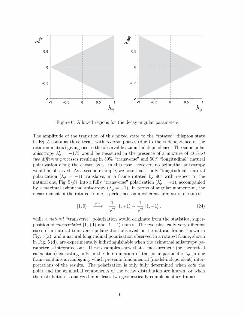
Since the magnitude of the “polar anisotropy”, λϑ, never exceeds 1 in any frame, wededuce the frame-independent inequalities

|λϕ| ≤1

2(1 + λϑ) , |λϑϕ| ≤

1

2(1− λϕ) , (22)

which imply the bounds |λϕ| ≤ 1 and |λϑϕ| ≤ 1. More interestingly, we can seethat |λϕ| ≤ 0.5 when λϑ = 0 and must vanish when λϑ → −1. The most generalphase space for the three angular parameters is represented in Fig. 6. There is analternative notation, widespread in the literature, where the coefficients λ, ν/2 andµ replace, respectively, λϑ, λϕ and λϑϕ. In that case, hence, we have |ν| ≤ 2.

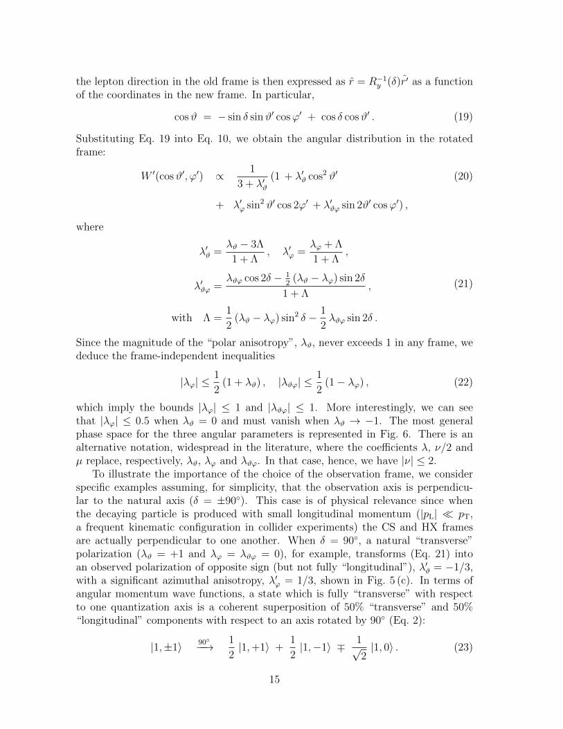
To illustrate the importance of the choice of the observation frame, we considerspecific examples assuming, for simplicity, that the observation axis is perpendicu-lar to the natural axis (δ = ±90◦). This case is of physical relevance since whenthe decaying particle is produced with small longitudinal momentum (|pL| � pT,a frequent kinematic configuration in collider experiments) the CS and HX framesare actually perpendicular to one another. When δ = 90◦, a natural “transverse”polarization (λϑ = +1 and λϕ = λϑϕ = 0), for example, transforms (Eq. 21) intoan observed polarization of opposite sign (but not fully “longitudinal”), λ′ϑ = −1/3,with a significant azimuthal anisotropy, λ′ϕ = 1/3, shown in Fig. 5 (c). In terms ofangular momentum wave functions, a state which is fully “transverse” with respectto one quantization axis is a coherent superposition of 50% “transverse” and 50%“longitudinal” components with respect to an axis rotated by 90◦ (Eq. 2):

|1,±1〉 90◦−−→ 1

2|1,+1〉 +

1

2|1,−1〉 ∓ 1√

2|1, 0〉 . (23)

15

λ φ

λθ

λ θφ

λφ

Figure 6: Allowed regions for the decay angular parameters.

The amplitude of the transition of this mixed state to the “rotated” dilepton statein Eq. 5 contains three terms with relative phases (due to the ϕ dependence of therotation matrix) giving rise to the observable azimuthal dependence. The same polaranisotropy λ′ϑ = −1/3 would be measured in the presence of a mixture of at leasttwo different processes resulting in 50% “transverse” and 50% “longitudinal” naturalpolarization along the chosen axis. In this case, however, no azimuthal anisotropywould be observed. As a second example, we note that a fully “longitudinal” naturalpolarization (λϑ = −1) translates, in a frame rotated by 90◦ with respect to thenatural one, Fig. 5 (d), into a fully “transverse” polarization (λ′ϑ = +1), accompaniedby a maximal azimuthal anisotropy (λ′ϕ = −1). In terms of angular momentum, themeasurement in the rotated frame is performed on a coherent admixture of states,

|1, 0〉 90◦−−→ 1√2|1,+1〉 − 1√

2|1,−1〉 , (24)

while a natural “transverse” polarization would originate from the statistical super-position of uncorrelated |1,+1〉 and |1,−1〉 states. The two physically very differentcases of a natural transverse polarization observed in the natural frame, shown inFig. 5 (a), and a natural longitudinal polarization observed in a rotated frame, shownin Fig. 5 (d), are experimentally indistinguishable when the azimuthal anisotropy pa-rameter is integrated out. These examples show that a measurement (or theoreticalcalculation) consisting only in the determination of the polar parameter λϑ in oneframe contains an ambiguity which prevents fundamental (model-independent) inter-pretations of the results. The polarization is only fully determined when both thepolar and the azimuthal components of the decay distribution are known, or whenthe distribution is analyzed in at least two geometrically complementary frames.

16

5 Effect of production kinematics on the observed

decay kinematics

Ideally, the dependence of the polarization on the momentum components of the pro-duced quarkonium should reflect the relative contribution of individual productionprocesses in different kinematic regimes, thereby providing information of fundamen-tal physical interest. However, the observations are, in general, affected by someexperimental limitations, which must be carefully taken in consideration. First, theframe-dependent polarization parameters λϑ, λϕ and λϑϕ can be affected by a strongexplicit kinematic dependence (encoded in the parameter δ in Eq. 21), reflecting thechange in direction of the chosen experimental axis (with respect to the “naturalaxis”) as a function of the quarkonium momentum. Second, detector acceptancesand event samples with limited statistics induce a dependence of the measurementon the distribution of events effectively accepted by the experimental apparatus.

To better explain the first problem, let us consider the HX and CS frames as theexperimental and natural frames, respectively. We start by calculating the angle be-tween the polarization axes of the CS and HX frames as a function of the quarkoniummomentum. The beam momenta in the “laboratory” frame (centre of mass of thecolliding particles), written in longitudinal and transverse components with respect

to the quarkonium direction, are ~P1 = −~P2 = P cos Θ ı‖ + P sin Θ ı⊥, where P istheir modulus and Θ is the angle formed by the quarkonium momentum with respectto the beam axis, defined in terms of the quarkonium momentum ~p as cos Θ = pL/p.When boosted to the quarkonium rest frame, the two vectors become (neglecting

the masses of the colliding particles) ~P ′1 = (γP cos Θ − βγP ) ı‖ + P sin Θ ı⊥ and~P ′2 = (−γP cos Θ − βγP ) ı‖ − P sin Θ ı⊥, where γ = E/m is the Lorentz factor of

the quarkonium state, and β = p/E =√

1− 1/γ2. The unit vectors indicating the zaxis directions in the HX and CS frames are

zHX = −~P ′1 + ~P ′2

| ~P ′1 + ~P ′2|=

~p

p,

zCS =P ′2 ~P

′1 − P ′1 ~P ′2

|P ′2 ~P ′1 − P ′1 ~P ′2|.

(25)

By definition, zHX = ı‖, while zCS can now be expressed as cos τ ı‖+ sin τ ı⊥, τ beingthe angle between the two axes:

cos τ =

1γ

cos Θ√1γ2

cos2 Θ + sin2 Θ=

mpLmT p

,

sin τ =sin Θ√

1γ2

cos2 Θ + sin2 Θ=

E pTmT p

.

(26)

We see that the result depends only on the momentum and mass of the quarkoniumstate (mT =

√m2 + p2T). The angle δ entering in Eq. 21, equal to τ in magnitude,

17

defines the positive rotation (respecting the right-hand rule) from one frame to theother. Its sign depends, therefore, on the exact conventions used for the orientationof the axes y and z of the polarization frames. In the convention where the y axis isdefined as

y =( ~P ′1 × ~P ′2)

| ~P ′1 × ~P ′2|(27)

and the z axis is defined by Eq. 25, with the “first” beam oriented as the laboratoryz axis, the positive rotation is the one bringing the HX axis to coincide with the CSaxis. We thus write, using Eq. 26,

δHX→CS = −δCS→HX = arccos

(mpLmT p

). (28)

Equation 21, containing terms of the form

sin2 δHX→CS = sin2 δCS→HX =p2TE

2

p2m2T

,

sin 2δHX→CS = − sin 2δCS→HX =2mpT pLE

p2m2T

,

(29)

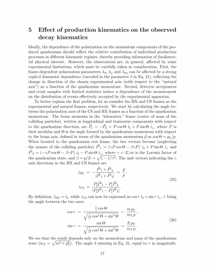
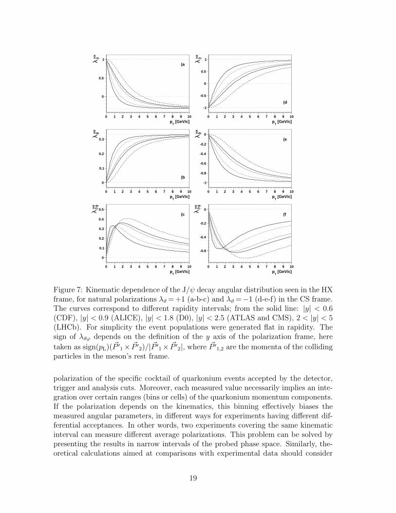
is now explicitly seen as a kinematic-dependent transformation.As an example, we show in Fig. 7 how natural J/ψ polarizations λϑ = +1 and

−1 in the CS frame (with λϕ = λϑϕ = 0 and no intrinsic kinematic dependence)translate into different pT-dependent polarizations measured in the HX frame in dif-ferent rapidity acceptance windows, representative of the acceptance ranges of severalTevatron and LHC experiments. Corresponding figures for the Υ(1S) case can beseen in Ref. [24]. The same results, except for a change in the sign of λϑϕ, the onlyparameter depending on the sign of the rotation angle, are obtained if the roles ofthe two frames are inter-exchanged.

The change of sign of the rapidity does not change the λϑ and λϕ curves. However,the sign of λϑϕ can change from positive to negative rapidity, depending on theconvention used for the orientation of the axes. If the axes are defined as in Eqs. 25and 27 at both positive and negative rapidity, always taking as “first” beam the onepositively oriented in the laboratory, λϑϕ (proportional to sin 2δ with 0 < δ < π) isforced to change sign when the rapidity changes sign. Any measurement integratingevents over a range in rapidity where the acceptance is symmetrical around zerowould, therefore, yield λϑϕ = 0. In order to avoid this cancellation, the axis definitionsin Eqs. 25 and 27 can be improved by inverting the orientations of y and zCS fornegative rapidity (correspondingly restricting the domain of the rotation angle to0 < δ < π/2).

Having seen how the strong kinematic dependence induced by the choice of theobservation frame can mimic and/or mask the fundamental (“intrinsic”) dependen-cies reflecting the production mechanisms, let us now discuss the additional problemscaused by common experimental limitations. Experiments can only measure the net

18

[GeV/c]T

p0 1 2 3 4 5 6 7 8 9 10

HX

ϑλ0

0.5

1(a

[GeV/c]T

p0 1 2 3 4 5 6 7 8 9 10

HX

ϑλ

-1

-0.5

0

0.5

1

(d

[GeV/c]T

p0 1 2 3 4 5 6 7 8 9 10

HX

ϕλ

0

0.1

0.2

0.3

(b

[GeV/c]T

p0 1 2 3 4 5 6 7 8 9 10

HX

ϕλ

-1

-0.8

-0.6

-0.4

-0.2

0(e

[GeV/c]T

p0 1 2 3 4 5 6 7 8 9 10

HX

ϕ

ϑλ

0

0.1

0.2

0.3

0.4

0.5(c

[GeV/c]T

p0 1 2 3 4 5 6 7 8 9 10

HX

ϕ

ϑλ

-0.6

-0.4

-0.2

0(f

Figure 7: Kinematic dependence of the J/ψ decay angular distribution seen in the HXframe, for natural polarizations λϑ = +1 (a-b-c) and λϑ =−1 (d-e-f) in the CS frame.The curves correspond to different rapidity intervals; from the solid line: |y| < 0.6(CDF), |y| < 0.9 (ALICE), |y| < 1.8 (D0), |y| < 2.5 (ATLAS and CMS), 2 < |y| < 5(LHCb). For simplicity the event populations were generated flat in rapidity. Thesign of λϑϕ depends on the definition of the y axis of the polarization frame, here

taken as sign(pL)( ~P ′1× ~P ′2)/| ~P ′1× ~P ′2|, where ~P ′1,2 are the momenta of the collidingparticles in the meson’s rest frame.

polarization of the specific cocktail of quarkonium events accepted by the detector,trigger and analysis cuts. Moreover, each measured value necessarily implies an inte-gration over certain ranges (bins or cells) of the quarkonium momentum components.If the polarization depends on the kinematics, this binning effectively biases themeasured angular parameters, in different ways for experiments having different dif-ferential acceptances. In other words, two experiments covering the same kinematicinterval can measure different average polarizations. This problem can be solved bypresenting the results in narrow intervals of the probed phase space. Similarly, the-oretical calculations aimed at comparisons with experimental data should consider

19

how the momentum distributions are distorted by the acceptances of those exper-iments. Alternatively, the predictions should avoid kinematic integrations or, evenbetter, be provided as event-level information to be embedded in the Monte Carlosimulations of the experiments. These considerations provide a further motivationfor reporting measurements and theoretical calculations in frame-independent terms,as we will discuss in the next section.

6 A frame-invariant approach

The general frame-transformation relations in Eq. 21 imply the existence of an invari-ant quantity, definable in terms of λϑ, λϕ and λϑϕ, in one of the following equivalentforms:

F{ci} =(3 + λϑ) + c1(1− λϕ)

c2(3 + λϑ) + c3(1− λϕ). (30)

An account of the fundamental meaning of the frame-invariance of these quantitiescan be found in Ref. [25]. We will consider here, specifically, the form

λ ≡ F{−3,0,1} =λϑ + 3λϕ1− λϕ

. (31)

In the special case when the observed distribution is the superposition of n “elemen-tary” distributions of the kind 1 + λ

(i)ϑ cos2 ϑ, with event weights f (i), with respect to

n different polarization axes, λ represents a weighted average of the n polarizations,insensitive to the orientations of the corresponding axes:

λ =n∑i=1

f (i)

3 + λ(i)ϑ

λ(i)ϑ

/ n∑i=1

f (i)

3 + λ(i)ϑ

. (32)

The determination of an invariant quantity is immune to “extrinsic” kinematic de-pendencies induced by the observation perspective and is, therefore, less acceptance-dependent than the standard anisotropy parameters λϑ, λϕ and λϑϕ.

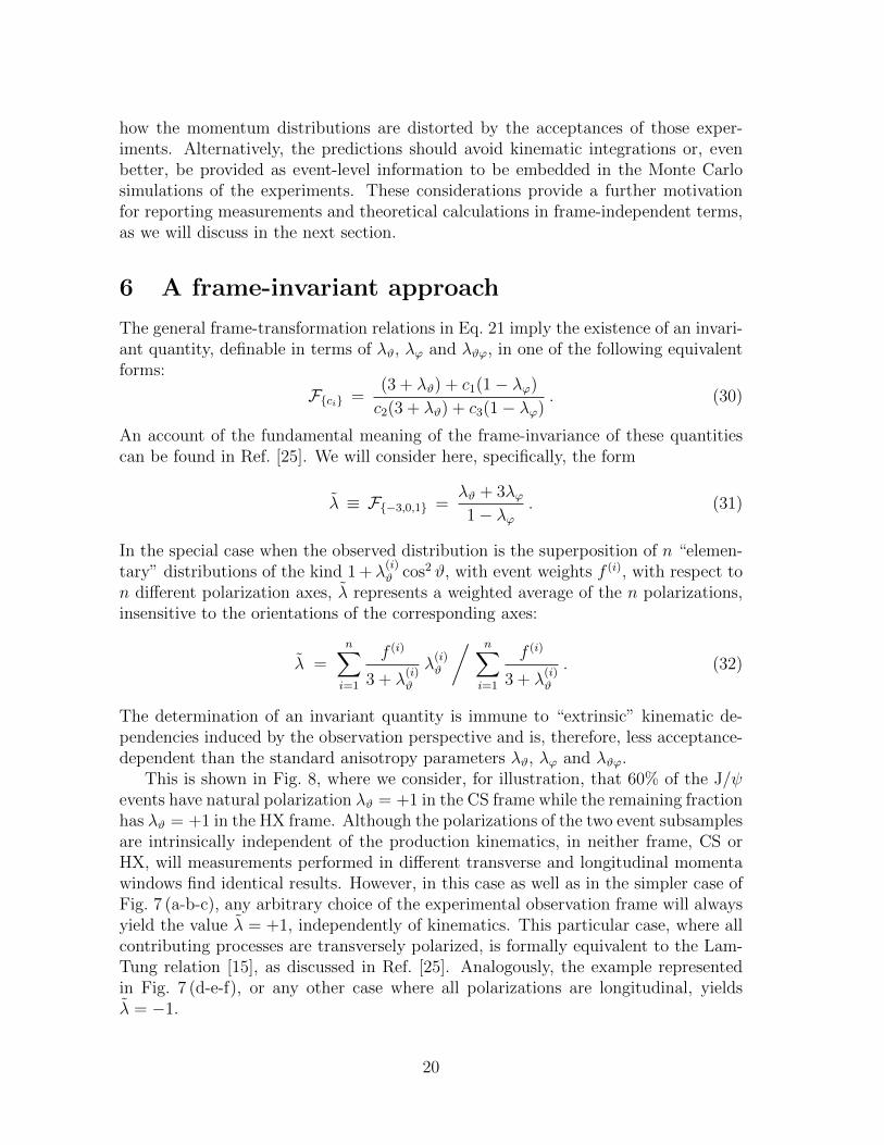
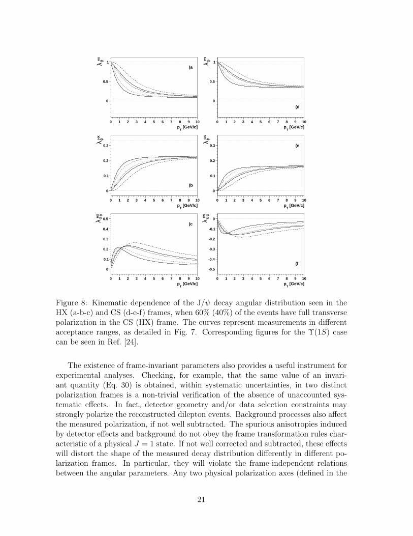
This is shown in Fig. 8, where we consider, for illustration, that 60% of the J/ψevents have natural polarization λϑ = +1 in the CS frame while the remaining fractionhas λϑ = +1 in the HX frame. Although the polarizations of the two event subsamplesare intrinsically independent of the production kinematics, in neither frame, CS orHX, will measurements performed in different transverse and longitudinal momentawindows find identical results. However, in this case as well as in the simpler case ofFig. 7 (a-b-c), any arbitrary choice of the experimental observation frame will alwaysyield the value λ = +1, independently of kinematics. This particular case, where allcontributing processes are transversely polarized, is formally equivalent to the Lam-Tung relation [15], as discussed in Ref. [25]. Analogously, the example representedin Fig. 7 (d-e-f), or any other case where all polarizations are longitudinal, yieldsλ = −1.

20

[GeV/c]T

p0 1 2 3 4 5 6 7 8 9 10

HX

ϑλ0

0.5

1(a

[GeV/c]T

p0 1 2 3 4 5 6 7 8 9 10

CS

ϑλ

0

0.5

1

(d

[GeV/c]T

p0 1 2 3 4 5 6 7 8 9 10

HX

ϕλ

0

0.1

0.2

0.3

(b

[GeV/c]T

p0 1 2 3 4 5 6 7 8 9 10

CS

ϕλ

0

0.1

0.2

0.3 (e

[GeV/c]T

p0 1 2 3 4 5 6 7 8 9 10

HX

ϕ

ϑλ

0

0.1

0.2

0.3

0.4

0.5(c

[GeV/c]T

p0 1 2 3 4 5 6 7 8 9 10

CS

ϕ

ϑλ

-0.5

-0.4

-0.3

-0.2

-0.1

0

(f

Figure 8: Kinematic dependence of the J/ψ decay angular distribution seen in theHX (a-b-c) and CS (d-e-f) frames, when 60% (40%) of the events have full transversepolarization in the CS (HX) frame. The curves represent measurements in differentacceptance ranges, as detailed in Fig. 7. Corresponding figures for the Υ(1S) casecan be seen in Ref. [24].

The existence of frame-invariant parameters also provides a useful instrument forexperimental analyses. Checking, for example, that the same value of an invari-ant quantity (Eq. 30) is obtained, within systematic uncertainties, in two distinctpolarization frames is a non-trivial verification of the absence of unaccounted sys-tematic effects. In fact, detector geometry and/or data selection constraints maystrongly polarize the reconstructed dilepton events. Background processes also affectthe measured polarization, if not well subtracted. The spurious anisotropies inducedby detector effects and background do not obey the frame transformation rules char-acteristic of a physical J = 1 state. If not well corrected and subtracted, these effectswill distort the shape of the measured decay distribution differently in different po-larization frames. In particular, they will violate the frame-independent relationsbetween the angular parameters. Any two physical polarization axes (defined in the

21

rest frame of the meson and belonging to the production plane) may be chosen toperform these “sanity tests”. The HX and CS axes are ideal choices at high pT andmid-rapidity, where they tend to be orthogonal to each other (in Eq. 29, sin2 δ → 1for pT � m and/or pT � |pL|). At forward rapidity and low pT, we can maximize thesignificance of the test by using the CS axis and the “perpendicular helicity axis” [26](which coincides with the helicity axis at zero rapidity and remains orthogonal tothe CS axis at nonzero rapidity). Given that λ is “homogeneous” to the anisotropyparameters, the difference λ(B) − λ(A) between the results obtained in two framesprovides a direct evaluation of the level of systematic errors not accounted in theanalysis.

7 Effect of intrinsic parton transverse momentum

In this section we describe how the geometry of the CS frame is related to the kine-matics of the production process. It can be recognized from Eq. 26 that the vectorzCS indicates the direction of the laboratory z axis (that is, the beam line) as seenin the quarkonium rest frame. In this frame, any length will be Lorentz contractedby a factor 1/γ along the quarkonium boost direction, but not along the transversedirections. In the quarkonium rest frame (as well as in the laboratory) the directionof the beam line coincides with the direction of the relative motion of the collidingpartons (“parton axis”), when their transverse momenta are neglected (and exactlywhen averaging a large sample of events). This approximation affects the experimen-tal determination of an angular distribution naturally of the kind 1 + λ∗ϑ cos2 ϑ∗ withrespect to the parton axis z∗. In the following considerations we fix a coordinate sys-tem having the z axis along the dilepton direction in the laboratory and the xz planecoinciding with the production plane. We then define the directions of the beam axisand of the parton axis in the laboratory as, respectively,

B = (sin Θ, 0, cos Θ) ,

B′ = (sin Θ′ cos Φ′, sin Θ′ sin Φ′, cos Θ′) ,(33)

where Θ and Θ′ are the angles they form with respect to the dilepton direction. Thepresence of the angle Φ′ denotes the fact that, due to the intrinsic transverse momentaof the partons, the vector B′ does not belong, in general, to the production plane.The angle ∆ between the two directions in the laboratory is given by

cos ∆ = sin Θ sin Θ′ cos Φ′ + cos Θ cos Θ′ . (34)

When boosted to the dilepton rest frame, the two vectors become

b =(sin Θ, 0, 1

γcos Θ)√

sin2 Θ + 1γ2

cos2 Θ,

b′ =(sin Θ′ cos Φ′, sin Θ′ sin Φ′, 1

γcos Θ′)√

sin2 Θ′ + 1γ2

cos2 Θ′

(35)

22

and the cosine of the angle between them

cos ζ =cos ∆− β2 cos Θ cos Θ′√

1− β2 cos2 Θ√

1− β2 cos2 Θ′. (36)

The rotation by ζ from the parton axis to the beam line axis transforms the polar-ization parameter λϑ according to the following expressions:

λCSϑ '

(1− 3 + λ∗ϑ

2〈sin2 ζ〉

)λ∗ϑ ,

λCSϕ ' λCS

ϑϕ ' 0 .

(37)

These transformations do not represent a simple rotation as Eq. 21. Indeed, themagnitude of the polar anisotropy decreases, while no significant azimuthal anisotropyarises. In fact, the rotation plane (formed by the parton and beam lines) does notcoincide with the experimentally defined production plane. The angle between thetwo planes changes from one event to the next, so that the azimuthal anisotropyderiving from the tilt between the “natural” polarization axis and the experimentalaxis tends to be smeared out in the integration over all events. Since cos ∆ ' 1 −12

sin2 ∆ and (approximately event-by-event, and exactly on average) cos Θ′ ' cos Θ,from Eq. 36 we obtain

〈sin2 ζ〉 ' 〈sin2 ∆〉1− β2 cos2 Θ

=E2

m2T

〈sin2 ∆〉 . (38)

Denoting by ~k1,2, ~k1,2T and E1,2 the total momenta, transverse momenta and energiesof the two partons in the laboratory, the laboratory angle ∆ satisfies

sin2 ∆ =(~k1T − ~k2T)2

(~k1 − ~k2)2' (~k1T − ~k2T)2

(E1 + E2)2(39)

and, on average,

〈sin2 ∆〉 ' 2〈~k2T〉(E1 + E2)2

, (40)

where we have defined the average parton squared transverse momentum as 〈~k2T〉 =

(〈~k21T〉+ 〈~k22T〉)/2.Considering now the specific case of Drell-Yan production at low pT, we can

assume an approximate equality between total parton energy and dilepton energy,E1+E2 ' E, and, moreover, 〈m2

T〉 ' m2+2〈~k2T〉. Combining Eqs. 37 (with λ∗ϑ = +1),38 and 40, we find that the measurement of the polarization of low-pT Drell-Yandileptons provides an estimate of the “effective” parton transverse momentum:

〈~k2T〉 'm2

2

1− λCSϑ

1 + λCSϑ

. (41)

23

The average Drell-Yan polarization λCSϑ = 1.008 ± 0.026 measured by E866 [13], in

proton-copper collisions for 〈m〉 ' 10 GeV/c2 and pT < 4 GeV/c, implies, therefore,that

〈~k2T〉 < 0.5 GeV2/c2 at 68% C.L. and

〈~k2T〉 < 1.0 GeV2/c2 at 95% C.L. .(42)

Tighter limits could be derived from precise low-mass measurements, given that thepolarization smearing effects are essentially proportional to m−2. Unfortunately, theexisting (pion-induced) measurements [27, 28], though very precise and extendingdown to 4 GeV/c2, present large azimuthal anisotropies of dubious interpretationand are scarcely suitable for this purpose.

We can now estimate the maximum magnitude of the smearing effects that canbe foreseen for the observable quarkonium polarization when the natural polarizationaxis is the parton axis. Combining again Eqs. 37, 38 and 40, this time with E1+E2 ≥E, we find that the magnitude of the polarization is reduced by the fraction∣∣∣∣λCS

ϑ − λ∗ϑλ∗ϑ

∣∣∣∣ .(3 + λ∗ϑ)〈~k2T〉m2 + p2T

. (43)

For example, it cannot be excluded, considering the limit in Eq. 42, that a fully trans-verse natural polarization of the J/ψ along the parton axis is reduced by as much as30%, for pT = 2 GeV/c, when observed in the CS frame. This smearing effect shouldbe one order of magnitude smaller for J/ψ mesons of pT = 10 GeV/c. On the otherhand, given the strong dependence of the effect on the dilepton mass, bottomoniumpolarization measurements are practically insensitive to the parton transverse mo-mentum even at low pT. This prediction is consistent with the already quoted E866results, showing Υ(2S + 3S) polarizations in the CS frame always compatible with+1, within a ∼ 15% uncertainty, in four pT bins between 0 and 4 GeV/c.

8 A few concrete examples

We conclude with some examples of measurements illustrating concepts described inthe previous sections.

We have already referred to the E866 measurement of a full transverse Υ(2S+3S)polarization in the CS frame. The result is represented in Fig. 9 (a), as a function ofpT. A similarly constant behaviour, consistent with a Drell-Yan-like polarization, hasbeen measured by this experiment as a function of xF, in the range [0, 0.5], confirmingthat the adoption of the CS frame is, in this case, an optimal choice. It is true that,in special kinematic conditions, the transverse polarization observed in one framecould, in reality, be the reflection of a natural longitudinal polarization in anotherframe, as shown in Fig. 7 (d). However, a maximal polarization independent of theproduction kinematics in the CS frame must directly reflect the spin configuration of

24

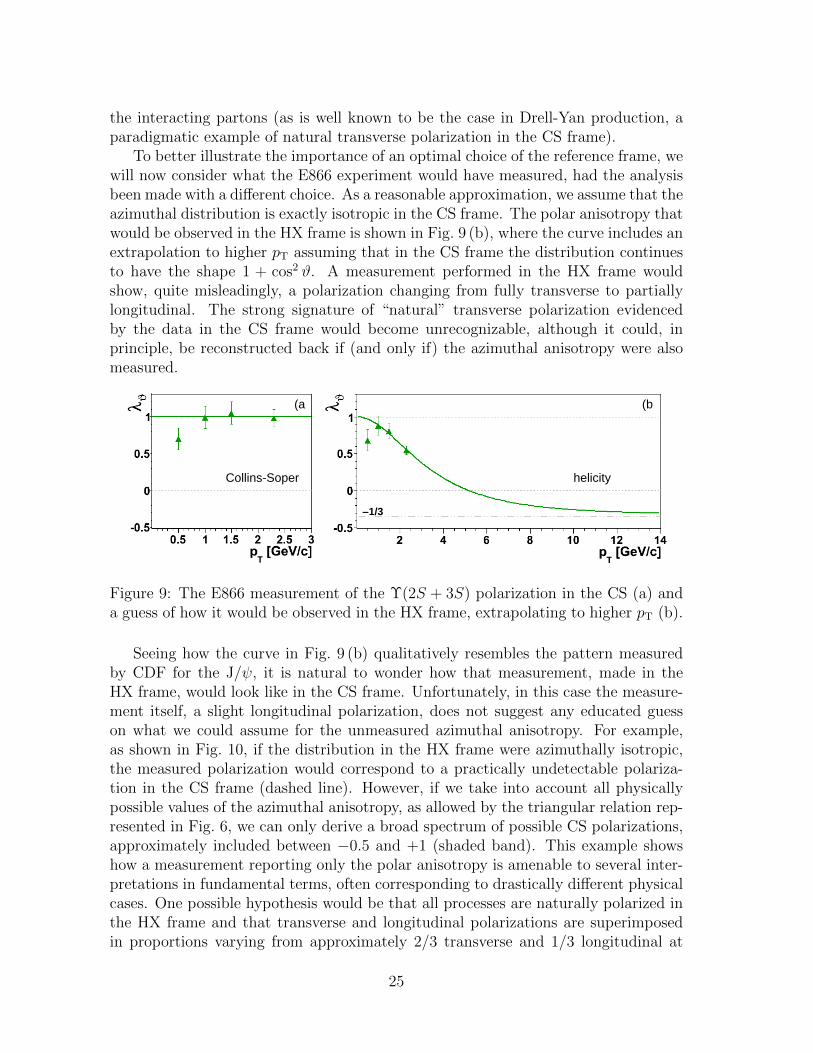
the interacting partons (as is well known to be the case in Drell-Yan production, aparadigmatic example of natural transverse polarization in the CS frame).

To better illustrate the importance of an optimal choice of the reference frame, wewill now consider what the E866 experiment would have measured, had the analysisbeen made with a different choice. As a reasonable approximation, we assume that theazimuthal distribution is exactly isotropic in the CS frame. The polar anisotropy thatwould be observed in the HX frame is shown in Fig. 9 (b), where the curve includes anextrapolation to higher pT assuming that in the CS frame the distribution continuesto have the shape 1 + cos2 ϑ. A measurement performed in the HX frame wouldshow, quite misleadingly, a polarization changing from fully transverse to partiallylongitudinal. The strong signature of “natural” transverse polarization evidencedby the data in the CS frame would become unrecognizable, although it could, inprinciple, be reconstructed back if (and only if) the azimuthal anisotropy were alsomeasured.

1/3

helicityCollins-Soper

(a (b

Figure 9: The E866 measurement of the Υ(2S + 3S) polarization in the CS (a) anda guess of how it would be observed in the HX frame, extrapolating to higher pT (b).

Seeing how the curve in Fig. 9 (b) qualitatively resembles the pattern measuredby CDF for the J/ψ, it is natural to wonder how that measurement, made in theHX frame, would look like in the CS frame. Unfortunately, in this case the measure-ment itself, a slight longitudinal polarization, does not suggest any educated guesson what we could assume for the unmeasured azimuthal anisotropy. For example,as shown in Fig. 10, if the distribution in the HX frame were azimuthally isotropic,the measured polarization would correspond to a practically undetectable polariza-tion in the CS frame (dashed line). However, if we take into account all physicallypossible values of the azimuthal anisotropy, as allowed by the triangular relation rep-resented in Fig. 6, we can only derive a broad spectrum of possible CS polarizations,approximately included between −0.5 and +1 (shaded band). This example showshow a measurement reporting only the polar anisotropy is amenable to several inter-pretations in fundamental terms, often corresponding to drastically different physicalcases. One possible hypothesis would be that all processes are naturally polarized inthe HX frame and that transverse and longitudinal polarizations are superimposedin proportions varying from approximately 2/3 transverse and 1/3 longitudinal at

25

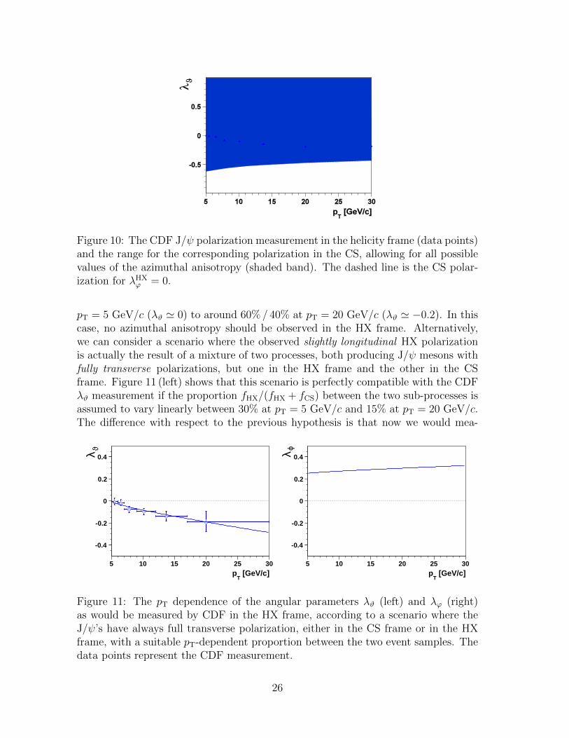
Figure 10: The CDF J/ψ polarization measurement in the helicity frame (data points)and the range for the corresponding polarization in the CS, allowing for all possiblevalues of the azimuthal anisotropy (shaded band). The dashed line is the CS polar-ization for λHX

ϕ = 0.

pT = 5 GeV/c (λϑ ' 0) to around 60% / 40% at pT = 20 GeV/c (λϑ ' −0.2). In thiscase, no azimuthal anisotropy should be observed in the HX frame. Alternatively,we can consider a scenario where the observed slightly longitudinal HX polarizationis actually the result of a mixture of two processes, both producing J/ψ mesons withfully transverse polarizations, but one in the HX frame and the other in the CSframe. Figure 11 (left) shows that this scenario is perfectly compatible with the CDFλϑ measurement if the proportion fHX/(fHX + fCS) between the two sub-processes isassumed to vary linearly between 30% at pT = 5 GeV/c and 15% at pT = 20 GeV/c.The difference with respect to the previous hypothesis is that now we would mea-

[GeV/c]T

p5 10 15 20 25 30

ϑλ

-0.4

-0.2

0

0.2

0.4

[GeV/c]T

p5 10 15 20 25 30

ϕλ

-0.4

-0.2

0

0.2

0.4

Figure 11: The pT dependence of the angular parameters λϑ (left) and λϕ (right)as would be measured by CDF in the HX frame, according to a scenario where theJ/ψ’s have always full transverse polarization, either in the CS frame or in the HXframe, with a suitable pT-dependent proportion between the two event samples. Thedata points represent the CDF measurement.

26

sure a significant azimuthal anisotropy, λϕ ' 0.3, as shown in Fig. 11 (right). Asan attempt to reconcile low-pT measurements with collider data, Ref. [10] describedone further conjecture, in which the polarization arises naturally in the CS frame,and becomes increasingly transverse with increasing total J/ψ momentum. Again, adirect measurement of λϕ (which, in this case, should be zero in the CS frame butpositive and increasing in the HX frame) would easily clarify the situation.

[GeV/c]T

p0 0.5 1 1.5 2 2.5 3 3.5 4 4.5 5

ϑλ

-0.8

-0.6

-0.4

-0.2

0

0.2

0.4

0.6

0.8

[GeV/c]T

p0 0.5 1 1.5 2 2.5 3 3.5 4 4.5 5

ϕλ-0.2

-0.1

0

0.1

0.2

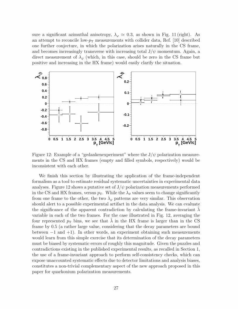
Figure 12: Example of a “gedankenexperiment” where the J/ψ polarization measure-ments in the CS and HX frames (empty and filled symbols, respectively) would beinconsistent with each other.

We finish this section by illustrating the application of the frame-independentformalism as a tool to estimate residual systematic uncertainties in experimental dataanalyses. Figure 12 shows a putative set of J/ψ polarization measurements performedin the CS and HX frames, versus pT. While the λϑ values seem to change significantlyfrom one frame to the other, the two λϕ patterns are very similar. This observationshould alert to a possible experimental artifact in the data analysis. We can evaluatethe significance of the apparent contradiction by calculating the frame-invariant λvariable in each of the two frames. For the case illustrated in Fig. 12, averaging thefour represented pT bins, we see that λ in the HX frame is larger than in the CSframe by 0.5 (a rather large value, considering that the decay parameters are boundbetween −1 and +1). In other words, an experiment obtaining such measurementswould learn from this simple exercise that its determination of the decay parametersmust be biased by systematic errors of roughly this magnitude. Given the puzzles andcontradictions existing in the published experimental results, as recalled in Section 1,the use of a frame-invariant approach to perform self-consistency checks, which canexpose unaccounted systematic effects due to detector limitations and analysis biases,constitutes a non-trivial complementary aspect of the new approach proposed in thispaper for quarkonium polarization measurements.

27

9 Summary and conclusions

Motivated by several puzzles affecting the existing measurements of quarkonium po-larization, we present in this paper a set of proposals which should improve theexperimental determination of the J/ψ and Υ polarizations. They are summarizedin the next paragraphs.

Measurements and calculations of vector quarkonium polarization should provideresults for the full dilepton decay angular distribution (a three-parameter function)and not only for the polar anisotropy parameter. Only in this way can the measure-ments and calculations represent unambiguous determinations of the average angularmomentum composition of the produced quarkonium state in terms of the three baseeigenstates, with Jz = +1, 0,−1.

It is advisable to perform the experimental analyses in at least two different polar-ization frames. In fact, the self-evidence of certain signature polarization cases (e.g.a full polarization with respect to a specific axis) can be spoiled by an unfortunatechoice of the reference frame, which can lead to artificial (“extrinsic”) dependenciesof the results on the kinematics and on the experimental acceptance.

The measured dependence of the polarization on the production kinematics isnecessarily influenced by the differential experimental acceptance, i.e. by the kine-matic distribution of the population of the accepted events. This problem, which isnot solved by acceptance corrections, can be minimized by providing the results innarrow cells in quarkonium rapidity and transverse momentum. Theoretical calcula-tions should be provided as event-level inputs to Monte Carlo generators which canbe tailored to the specific performance capabilities of each experiment.

The decay angular distribution can be characterized by a frame-independent quan-tity, such as λ, calculable in terms of the polar and azimuthal anisotropy parameters.The existence of such frame-invariant quantities can be used during the data analy-sis phase to perform self-consistency checks that can expose previously unaccountedbiases, caused, for instance, by the detector limitations or by the event selectioncriteria.

Besides providing a much needed control over systematic experimental biases, thevariable λ also provides relevant physical information: it characterizes the shape ofthe angular distribution, reflecting “intrinsic” spin-alignment properties of the decay-ing state, irrespectively of the specific geometrical framework chosen by the observer.For instance, we obtain λ = +1 for the shapes shown in Fig. 5 (a) and (c), andλ = −1 for the shapes shown in the panels (b) and (d). A very important advantageof re-expressing the frame-dependent polar and azimuthal anisotropies in terms of aframe-invariant quantity is the exact cancellation of extrinsic dependencies on kine-matics and acceptances, enabling more robust comparisons with other experimentsand with theory. The calculation of λ requires, anyhow, the determination of the fulldecay distribution in a chosen reference frame and, obviously, does not replace thisstandard procedure. Moreover, the three frame-dependent parameters (λϑ, λϕ andλϑϕ) can provide information on the direction of the spin-alignment of the decayingparticle (when this direction is univocally defined) and, therefore, on the topological

28

properties of the dominant production mechanism. For instance, the measurementof a full transverse polarization in the CS frame represents a direct observation ofthe spin alignments of the interacting partons, as we know from Drell-Yan produc-tion. On the other hand, in the presence of a superposition of production processeswith polarizations along different axes, measuring the frame-dependent anisotropieswill not provide, in general, much information on the polarizations involved or ontheir natural alignment directions, while the value of λ will immediately tell us if theprocesses involved have a predominantly transverse or longitudinal nature.

Stripped-down analyses which only measure the polar anisotropy in a single ref-erence frame, as often done in past experiments, give more information about theframe selected by the analyst (“is the adopted quantization direction an optimalchoice?”) than about the physical properties of the produced quarkonium (“alongwhich direction is the spin aligned, on average?”). For example, a natural longitu-dinal polarization will give any desired λϑ value, from −1 to +1, if observed froma suitably chosen reference frame. Lack of statistics is not a reason to “reduce thenumber of free parameters” if the resulting measurements become ambiguous. Theforthcoming measurements of quarkonium polarization in proton-proton collisions atthe LHC have the potential of providing a very important step forward in our under-standing of quarkonium production, if the experiments adopt a more robust analysisframework, incorporating the ideas presented in this paper.

P.F., J.S. and H.K.W. acknowledge support from Fundacao para aCiencia e a Tecnologia, Portugal, under contracts SFRH/BPD/42343/2007,CERN/FP/109343/2009 and SFRH/BPD/42138/2007.

References

[1] N. Brambilla et al. (QWG Coll.), CERN Yellow Report 2005-005, hep-ph/0412158, and references therein.

[2] F. Abe et al. (CDF Coll.), Phys. Rev. Lett. 79, 572 (1997).

[3] G.T. Bodwin, E. Braaten and G.P. Lepage, Phys. Rev. D 51, 1125 (1995); Phys.Rev. D 55, 5853E (1997).

[4] J.P. Lansberg, Eur. Phys. J. C 61 (2009) 693.

[5] M. Beneke and M. Kramer, Phys. Rev. D 55, 5269 (1997).

[6] A.K. Leibovich, Phys. Rev. D 56, 4412 (1997).

[7] E. Braaten, B.A. Kniehl and J. Lee, Phys. Rev. D 62, 094005 (2000).

[8] A. Abulencia et al. (CDF Coll.), Phys. Rev. Lett. 99, 132001 (2007).

[9] P. Faccioli, C. Lourenco, J. Seixas, and H.K. Wohri, J. High Energy Phys. 10,004 (2008).

[10] P. Faccioli, C. Lourenco, J. Seixas and H.K. Wohri, Phys. Rev. Lett. 102, 151802(2009).

29

[11] D. Acosta et al. (CDF Coll.), Phys. Rev. Lett. 88, 161802 (2002).

[12] V.M. Abazov et al. (D0 Coll.), Phys. Rev. Lett. 101, 182004 (2008).

[13] C.N. Brown et al. (E866 Coll.), Phys. Rev. Lett. 86, 2529 (2001).

[14] T. Affolder et al. (CDF Coll.), Phys. Rev. Lett. 85, 2886 (2000).

[15] C.S. Lam and W.K. Tung, Phys. Rev. D 18, 2447 (1978).

[16] M. Artuso et al. (CLEO Coll.), Phys. Rev. D 80, 112003 (2009).

[17] T.A. Armstrong et al. (E760 Coll.), Phys. Rev. D 48, 3037 (1993); M. Ambro-giani et al. (E835 Coll.), Phys. Rev. D 65, 052002 (2002).

[18] M. Ambrogiani et al. (E835 Coll.), Phys. Lett. B 610, 177 (2005).

[19] E. Braaten and T.C. Yuan, Phys. Rev. Lett. 71, 1673 (1993).

[20] H. Fritzsch, Phys. Lett. B 67, 217 (1977); F. Halzen, Phys. Lett. B 69, 105(1977).

[21] K. Gottfried and J.D. Jackson, Nuovo Cim. 33, 309 (1964).

[22] J.C. Collins and D.E. Soper, Phys. Rev. D 16, 2219 (1977).

[23] D.M. Brink and G.R. Satchler, “Angular momentum” (Third Edition), Claren-don Press, Oxford (1993).

[24] P. Faccioli, C. Lourenco and J. Seixas, Phys. Rev. D 81, 111502(R) (2010).

[25] P. Faccioli, C. Lourenco and J. Seixas, arXiv:1005.2601 [hep-ph]; Phys. Rev.Lett., in print.

[26] E. Braaten, D. Kang, J. Lee and C. Yu, Phys. Rev. D 79, 014025 (2009).

[27] S. Falciano et al. (NA10 Coll.), Z. Phys. C 31, 513 (1986).

[28] J.S. Conway et al. (E615 Coll.), Phys. Rev. D 39, 92 (1989).

30