Towards New Open Economy Ma · PDF file3 After Obstfeld and Rogoff (1995) the theoretical literature in open economy macroeconomics has been evolving along different directions depending

1

Comments welcome

Towards New Open Economy Macroeconometrics *

Fabio GhironiΗ

Boston College

First draft: August 9, 1999 This draft: February 23, 2000

Abstract

I estimate the structural parameters of a small open economy model using data from Canada and the United States. The model improves upon the recent literature in open economy macroeconomics from an empirical perspective. I estimate parameters by using non-linear least squares at the single-equation level. Estimates of most parameters are characterized by small standard errors and are in line with the findings of other studies. I also develop a plausible way of constructing measures for non-observable variables. To verify if multiple-equation regressions yield significantly different estimates, I run full information maximum likelihood, system-wide regressions. The results of the two procedures are similar. Finally, I illustrate a practical application of the model, showing how a shock to the U.S. economy is transmitted to Canada under an inflation targeting monetary regime.

Keywords: Open economy macroeconometrics; Stationarity; Shocks transmission JEL Classification: C51, F41

* This paper is based on Chapter 3 of my Ph.D. Dissertation at U.C. Berkeley. It contains part of the material I presented in my job seminars in 1999. I thank the members of my Dissertation Committee—Barry Eichengreen, Maury Obstfeld, David Romer, and Andy Rose—as well as David Card and Francesco Giavazzi, for their suggestions and encouragement. I thank for comments and useful conversations Gianluca Benigno, Laura Bottazzi, Petra Geraats, and Paolo Manasse. I am also grateful to seminar audiences at Berkeley, the Board of Governors, Boston College, Brown, Florida International University, George Washington University, Iowa State, Johns Hopkins, the New York Fed, NYU, Tilburg University, UCLA, University of Pittsburgh, and Washington University. I thank George di Giovanni, Julian di Giovanni, and Philip Oreopoulos for helping me overcome the vagaries of the Internet to gather data on the Canadian economy in the Summer of 1998. Andrei Levchenko provided outstanding research assistance. Remaining errors are of course my own. Financial support from the Institute of International Studies at U.C. Berkeley and the MacArthur Foundation during academic years 1997/1998 and 1998/1999 is gratefully acknowledged. Much work on this paper was undertaken while I was at the Federal Reserve Bank of New York. Η Address for correspondence: Department of Economics, Boston College, Carney Hall 131, Chestnut Hill, MA 02467-3806. E-mail: [email protected]. Phone: (617) 552-3686. Fax: (617) 552-2308. URL: http://FMWWW.bc.edu/EC-V/Ghironi.fac.html.

2

1. Introduction

I estimate the structural parameters of a small open economy model using data from Canada andthe United States. The model improves upon the recent literature in open economymacroeconomics from an empirical perspective. It is described in detail in Ghironi (1999a). Iestimate parameters by using non-linear least squares at the single-equation level. Calibration isused only when the regressions do not yield sensible estimates. The sensibility of the parametervalues obtained in this way is verified by comparing them to the findings of a large empiricalliterature. Estimates of most parameters turn out to be characterized by small standard errors andare in line with the findings of other studies. Illustrating a plausible way of constructing measuresfor non-observable variables is a contribution of this paper. To verify if multiple-equationregressions yield significantly different estimates, I also run full information maximum likelihoodsystem-wide regressions taking the estimates from the single-equation procedure as initial values.The results of the two procedures are similar.

I then illustrate the functioning of the model by using the parameter estimates to calibrateit and analyze the transmission of a shock to U.S. GDP to the Canadian economy under inflationtargeting, the monetary regime currently followed by the Bank of Canada. When doing thisexercise, I combine the theoretical model of the Canadian economy with a simple VAR that tracesthe comovements of U.S. variables affecting Canada directly. The exercise illustrates the role ofmarkup and relative price dynamics in the model. The latter does a better job than the flexible-price framework used by Schmitt-Grohé (1998) at explaining the transmission of U.S. cycles toCanada.1

The structure of the paper is as follows. Section 2 outlines the main features of the modeland compares it to the existing literature. Section 3 presents the main log-linear equations of themodel and illustrates the estimation procedure. Section 4 is devoted to the example. Section 5concludes.

2. The Model and the Literature

After a long-lasting predominance of non-microfounded Keynesian models, the publication ofObstfeld and Rogoff’s “Exchange Rate Dynamics Redux” in 1995 opened the way to a newgeneration of models of macroeconomic interdependence. These models combine a rigorouslymicrofounded approach with analytical tractability. The literature following Obstfeld and Rogoff’swork has been mainly theoretical. Papers in this literature are said to belong to the so-called “newopen economy macroeconomics.”2 However, empirical performance will ultimately decidewhether this new generation of models will supplant the time-honored Mundell-Fleming-Dornbusch framework as the main tool for understanding interdependence and for formulatingpolicy advice. This paper is a contribution in that direction. It provides—to the best of myknowledge—the first comprehensive attempt at estimating an open-economy model in line withthe recent developments in the theoretical literature and it illustrates how to use the model in anempirical way. For this reason, the paper can be thought of as an initial contribution to “new openeconomy macroeconometrics.” 1 In Ghironi (1999b), I evaluate the performance of the Canadian economy under alternative monetary rules whenCanada is subject to different sources of volatility. Because the exercise relies on estimates of the structuralparameters of the model, the bearing of the Lucas critique on the results is weakened.2 For a survey, see Lane (1999).

3

After Obstfeld and Rogoff (1995) the theoretical literature in open economymacroeconomics has been evolving along different directions depending also on the role attributedto the current account. The latter plays a crucial role in the transmission of shocks in the originalObstfeld-Rogoff model. But this comes with a major problem of the framework that makes theconclusions questionable from a theoretical and empirical perspective, namely the absence of awell defined endogenously determined steady state. In the model, the position of the domestic andforeign economies that is taken to be the steady state in the absence of shocks is a point to whichthe economies never return following a disturbance. The consumption differential betweencountries follows a random walk. So do an economy’s net foreign assets. Whatever level of assetholdings materializes in the period immediately following a shock becomes the new long-runposition of the current account, until a new shock happens.

Determinacy of the steady state and stationarity fail because the average rate of growth ofthe economies’ consumption in the model does not depend on average holdings of net foreignassets. Hence, setting consumption to be constant is not sufficient to pin down a steady-statedistribution of asset holdings. This makes the choice of the economy’s initial position for thepurpose of analyzing the consequences of a shock arbitrary. When the model is log-linearized, oneis actually approximating its dynamics around a “moving steady state.” The reliability of the log-linear approximation is low, especially for analyses whose time horizon is longer than a one-period exercise, because variables wander away from the initial steady state. De facto, one cannotperform any stochastic analysis. The inherent unit root problem complicates empirical testing. Andthe long-run non-neutrality of money that characterizes the results can be attacked on empiricalgrounds.

Scholars of international macroeconomics soon recognized the problem. Some decided todismiss it.3 Others tried to finesse the current account issue in various ways. For example,Corsetti and Pesenti (1998) propose a model in which the importance of the current account is de-emphasized. They achieve this by assuming unitary intratemporal elasticity of substitution betweendomestic and foreign goods in consumption. Under this assumption, the current account does notreact to shocks, and thus plays no role in their transmission. The justification Corsetti and Pesentioffer for claiming that this is not a bad approximation of reality when the purpose is providingnormative conclusions is that, even when the current account does move, the difference itsmovements make for a country’s welfare is only second order. The Corsetti-Pesenti simplificationhas proved very successful in the literature. It makes it possible to solve the model without havingto resort to log-linearization—a big tractability gain—and yields interesting theoretical insights.Several papers have later adopted the approach, including Benigno P. (1999) and Obstfeld andRogoff (1998, 2000).

However, the Corsetti-Pesenti model shares the indeterminacy of the steady state with theoriginal Obstfeld-Rogoff framework. There too, setting consumption to be constant does not pindown a steady-state international distribution of asset holdings, for the same reason mentionedabove. The choice of a zero-asset initial equilibrium, combined with the assumption on theelasticity of substitution between foreign and domestic goods, allows Corsetti and Pesenti—andthe followers of their approach—to shut off the current account channel. This opens the way tostochastic analysis in a highly tractable framework, but at a large cost in terms of realism. Anyinitial position different from the zero-asset equilibrium brings the non-stationarity of the modelback to the surface. 3 I do so in Ghironi (2000).

4

An alternative way of dealing with the non-stationarity problem by shutting off the currentaccount channel consists of assuming that financial markets are complete. Because of perfect risksharing in complete markets, the current account does not react to shocks. This is the approachfollowed by Benigno G. (1999) and Gali and Monacelli ( 1999). This too yields highly tractablemodels suitable for stochastic analysis but at a potentially high cost in terms of realism. As arguedby Obstfeld and Rogoff (1995, 1996 Ch. 10), the complete markets assumption also seems atodds with the presence of real effects of unanticipated monetary shocks in a world in which pricesare sticky.

The Corsetti-Pesenti simplification or the complete markets assumption are now settingthe trend in the theoretical literature. But there are reasons to believe that these approaches riskmissing very important features of economic interdependence. For example, the recent dynamicsof the U.S. current account suggest that the latter may play an important role in generatinginterdependence between the United States and the rest of the world. Hence, one may want to beable to analyze interdependence formally without shutting off the current account while at thesame time preserving a reasonable degree of tractability.

In Ghironi (1999a), I develop a tractable perfect-foresight, two-country, generalequilibrium model that offers a solution to the indeterminacy/non-stationarity issue that is notshutting off the current account channel.

I do so by changing the demographic structure relative to the representative agentframework used in most of the literature. I follow Weil (1989) in assuming that the worldeconomy consists of distinct infinitely lived households that come into being on different dates andare born owning no assets. This demographic structure, combined with the assumption that newlyborn agents have no financial wealth, allows the model to be characterized by a steady state towhich the world economy returns over time following temporary shocks. Agents consume; holdmoney balances, bonds, and shares in firms; and supply labor.

Because the model is stationary around an endogenously determined steady state, I do notrely on the Corsetti-Pesenti simplifying assumption that removes current account effects nor Iassume complete markets. The current account does play a role in my model. Whether or not thisis important can then be subject of empirical investigation.

As do most models in the recent open macro literature, I assume that a continuum ofgoods is produced in the world by monopolistically competitive firms, each of which produces asingle differentiated good. Preferences for consumption goods are identical in the two countries,and the law of one price and consumption-based Purchasing Power Parity (PPP) hold.4

The failure of stationarity is not the only problem of several existing models. Theassumption of one-period price rigidity that characterizes several exercises is not appealing forempirical purposes. The absence of investment and capital accumulation from the models limitstheir appropriateness for thorough empirical investigations of current-account behavior and of theconsequences of alternative policy rules for medium to long-run dynamics.5

4 Engel and Rogers (1996) provide evidence of deviations from the law of one price between the U.S. andCanada—the economies on which I focus in my empirical exercise. This notwithstanding, I limit myself to thesimpler case, to focus on other directions along which the original Obstfeld-Rogoff framework can be extended.5 Bergin (1997) extends the Obstfeld-Rogoff framework to allow for investment and capital accumulation andperforms calibration exercises. Kollmann (1999) analyzes the implications of nominal rigidity for the behavior ofasset prices. Nonetheless, the arbitrariness of the point around which to log-linearize is not resolved in theirmodels.

5

In the model I propose, firms produce using labor and physical capital. Capital isaccumulated via investment, and new capital is costly to install as in a familiar Tobin’s q model.The presence of monopoly power has consequences for the dynamics of employment, byintroducing a wedge between the real wage index and the marginal product of labor.

I assume that firms face costs of adjusting the price of their outputs. I choose a quadraticspecification for these costs, as in Rotemberg (1982). This specification produces aggregatedynamics similar to those induced by staggered price setting a’ la Calvo (1982). It also generatesa markup endogenous to the conditions of the economy as long as the latter is not in steady state.6

The dynamics of the markup play an important role in business cycle fluctuations, consistent withthe analysis of Rotemberg and Woodford (1990). The dynamics of the real wage are not tied tothose of the marginal product of labor.

My model lends itself naturally to empirical analysis and stochastic applications. Althoughthe model is potentially a tool for analyzing bilateral interdependence between countries, in its firstempirical implementation, I focus on a small open economy case in order to make use of a set ofsimplifying exogeneity assumptions. The home economy is identified with Canada, which is smalland open when compared to the rest-of-the-world economy, approximated by the United States.For this reason, when presenting the model, I assume that the home economy is much smaller thanthe foreign one. The small open economy assumption implies that foreign variables and worldaggregates are given from the perspective of the domestic economy. Exogeneity of foreignvariables with respect to home’s provides a set of restrictions I use in my empirical analysis.

3. Estimating the Log-Linear Economy

The microfounded setup of the model can be found in Ghironi (1999a), along with the solutionfor the steady state. In this section, I present the log-linear equations that govern the dynamics ofthe home economy—Canada—following small perturbations to the steady state and I illustrate aplausible approach to the estimation of the structural parameters of the model. For consistencywith Ghironi (1999b), where I focus on monetary issues for Canada, I assume that fiscal policyvariables are kept at their steady-state levels in what follows, and drop them from the log-linearized equations. Unobservable variables appear in some of these equations. An important partof this section deals with my empirical approach to the issue of measuring these variables.

The strategy used to estimate the structural parameters of the model consists of two steps.I first run single equation regressions. These—and the use of calibration when the regressions failto yield sensible results—provide me with a set of baseline estimates. To verify the reliability ofthese estimates, I use them as starting values for full information maximum likelihood regressionsof the systems of the firms’ and consumers’ first-order conditions.

Rotemberg and Woodford (1997) pursue an alternative approach to the issue of estimatinga dynamic microfounded model. They run a three-variate recursive VAR for the U.S. economyand estimate the structural parameters of their model by calibrating them so that the model’simpulse responses match the VAR’s. I did not follow this strategy for two reasons. First, I find itad hoc. Second, Rotemberg and Woodford’s model is significantly simpler than mine, and itinvolves a smaller number of parameters. If I had followed their strategy, I would have faced the

6 Carré and Collard (1997) adopt a similar approach, as well as Ireland (1997, 1999) in a closed economy setting.G. Benigno (1999) and P. Benigno (1999) rely on Calvo-type mechanisms.

6

problem that a possibly large number of combinations of sensible parameter values are likely toallow the model to match the VAR’s responses.

Cushman and Zha (1997) use the small open economy assumption to estimate a structuralVAR of the U.S. and Canadian economies. Block exogeneity helps identify Canadian monetaryshocks. However, no underlying model is estimated. Working along their lines, I could have run alarge scale identified VAR a’ la Leeper, Sims, and Zha (1996), but this would have left me withthe problem of mapping the estimates of the VAR coefficients into estimates of the structuralparameters of my model.

For these reasons, the strategy I decided to follow seems to be a reasonable way to let thedata reveal something about parameter values. As it turns out, the strategy is fairly successful. Asthe reader will find out, I have to rely on pure calibration only in one case in the single-equationprocedure, and the system-wide regressions yield estimates that are similar to those obtained inthe first step. In addition, the estimates are in line with the findings of a large body of empiricalliterature.

3.a. Investment, Pricing, and Labor Demand

The log-linear production function is:( )y RP k L Zt t t t t= + + − +γ γ1 , (3.1)

where arial variables denote percentage deviations from the initial steady state, y is detrendedaggregate per capita GDP, RP is the price of the representative domestic good in terms of theconsumption bundle ( ( ) PipRP≡ ), k is detrended aggregate per capita capital, L is aggregateper capita labor demand, and Z is a productivity shock.

The elasticity of Canadian output with respect to hours worked—1− γ —is the firststructural parameter I estimate. The data come from the CANSIM database and from the IMFInternational Financial Statistics. I use quarterly data, consistent with the purpose of working atbusiness cycle frequencies. Availability problems for some crucial series force me to restrictattention to the sample period 1980:1-1997:4. I construct the trend series ( ) 11 −+= tt EgE by

assuming that g is the average rate of growth of Canadian real GDP per capita during the sampleperiod and letting E1980 2 1: = . Steady-state levels of variables are calculated as the unconditionalmeans of the series over the sample period. Variables in the regressions are defined as percentagedeviations from the steady state, to match the concepts in the model.

Regressing Canadian GDP on the ratio of the industrial price index to the CPI, on thecapital stock, on hours, and on a set of seasonal dummies, yields an estimate for 1− γ ofapproximately .9.7 This is a high value for the elasticity of output to hours. However, it seemsreasonable that GDP be much more sensitive to hours than capital on a quarterly basis. For thisreason, I will take .9 to be the baseline value of 1− γ in what follows. The log-linear equation that determines detrended investment at each point in time is:

7 The standard error of the estimate is .067, so that the estimated coefficient is highly significant. The estimatedcoefficient on capital in an unrestricted regression is .06, and it is hardly significant. The R2 of the regression is.82, and the Durbin-Watson statistic is 1.3. Alternative specifications of the regression improved the significanceof capital and raised the Durbin-Watson statistic somewhat, yielding estimates for 1− γ in the range .86 to .93.

7

( )( ) ( )[ ]( )( ) ( )[ ]inv k qt t t

n g

n g− =

+ + + − −

+ + − −

1 1 1 1

1 1 1

η δη δ

. (3.2)

n is the rate of growth of population, η measures the size of the cost of adjusting the capitalstock, δ is the rate of depreciation of capital, and q is Tobin’s q. From the law of motion fordetrended aggregate per capita capital, it follows that:

( )( ) ( )( )( ) ( )k k inv kt t t t

n g

n g+ − =

+ + − −+ +

−1

1 1 1

1 1

δ. (3.3)

The change in aggregate per capita capital between t and t + 1 is faster the larger investment andthe smaller the stock of capital at time t.

Log-linearizing the Euler equation for capital accumulation in detrended aggregate percapita terms gives:

( )( ) ( )( ) ( )[ ]( ) ( ),1

111

111

1~11

0

2

11100

0011 +++++++ −

+−−+++−+

+−+

+−+−= tttttttt

rq

gn

rkq

Lw

rkinvkLwqrq

δηγ

γδ

(3.4)where r~ is the real interest rate—the steady-state level of which is r—and w is the detrended realwage. 8 A bar and the subscript 0 denote the constant steady-state level of the correspondingvariable.

Tobin’s q is one of the variables in the model that pose significant measurement problems.I construct a measure for the economy-wide q for Canada as follows.

Given the expression for the individual firm’s q in Ghironi (1999a), it is possible to showthat q q qt

it t= = , where qt is measured using aggregate data, and qt is defined in terms of

detrended aggregate per capita variables:

( )( )[ ] ( ) ( )( )[ ]11

, 1111

11 +

∞

+=

− ++

−−

Ψ+++= ∑ t

tss

Fs

s

tssttt kgnygnRvq τ ,

v V E Pt t t t≡ is the detrended aggregate per capita equity value of the home economy; the

discount factor Rt s, is defined by ( )∏+=

+≡s

tuust rR

1, 11 and ttR , is interpreted as 1; Ψ is the

markup charged by firms over marginal costs; and τF is the rate of taxation of firms’ revenues. Inow define average q and the “adjustment for monopoly power” as:

( )( )

( )( )[ ] ( )( )( ) .

11

11

11

,11 1

1,

1 +

∞

+=

−

+ ++

−−

Ψ++

≡++

≡∑

t

tss

Fs

s

tsst

t

t

tAVGt

kgn

ygnR

adjkgn

vq

τ(3.5)

When substitutability across goods is perfect, Ψ reduces to 1/(1 - τF ), and marginal and averageq coincide—the familiar Hayashi (1982) result. Measuring average q does not pose significantproblems. Quarterly data for aggregate equity and firms’ net capital assets since 1980:1 areavailable for the Canadian economy, and—together with the series for the CPI—they make itpossible to obtain the desired measure. n is calculated as the average rate of growth of theCanadian population over the sample.

8 A tilde over an arial rate denotes the percentage deviation of the gross rate from its steady-state level.

8

Measuring the adjustment term is harder. First, in reality agents do not have perfectforesight. adjt is actually an expectation conditional on the information set available to firms attime t of the present discounted value of the “monopoly effect” from t + 1 on. Second, this effectdepends on the behavior of the markup, which itself needs to be estimated.

The equilibrium value of the markup can be written as ( ) ( )tttt Lwyγ−=Ψ 1 . Given the

estimate of the elasticity of GDP with respect to hours obtained above, I can calculate a baselineseries of the markup using this expression. The results suggest that the Canadian economy ischaracterized by a fairly small degree of monopoly power at the aggregate level. The averagelevel of the markup implied by the data is 1.11. Figure 1 shows the series of the growth rate of themarkup over the sample period and the series of the growth rate of hours. As expected, andconsistent with the evidence for the U.S. economy in Rotemberg and Woodford (1990), themarkup is strongly countercyclical. This is a feature of the model that is important in the analysis

of the model’s dynamics. Because the steady-state markup is given by ( )( )[ ]Ψ0 01 1= − −θ θ τ F ,

where τ 0F is the unconditional mean of the series of the tax rate on firms’ revenues, it is possible

to use this result to obtain an initial estimate of θ around 12.08.9

I now define the variable ( )( )[ ] ( ) ( )[ ] sFss

tsstst ygnR τ−−Ψ++≡Ω −

1111,, . I measure the

relevant real interest rate with a series of the ex post real rate on Canadian T-Bills, calculated bydeflating the nominal rate with CPI inflation.10 As Figure 2 shows, if the series of the variableΩ t s, is plotted, the diagram suggests that the process for Ω t s, is non-stationary: the variance of

the series drops to zero as time goes by.11 When discounted back to the initial date by making use

of the real interest rate, the variable ( )( )[ ] ( ) ( )[ ] sFss

tss ygnX τ−−Ψ++≡ − 1111 decays towards

zero, i.e., discounting by the real interest rate introduces a trend in Ω t s, .

It is possible to show that ( ) ( ) ( ) 1,11 1,1,1, +≥∀Ω+=Ω=Ω+ −−− tsgXXr stXsstsssts ,

where ( )g X XsX

s s≡ −−1 1. Averaging the ratio X Xs s−1 over the sample, it can be argued that

the following process is a reasonable approximation for the behavior of Ω t s, in a stochastic

setting: ( ) ( )[ ] sstX

st zrg +Ω++=Ω −1,, 11 ω , where z is a series of unanticipated disturbances.

Writing the process for Ω t s, in this form makes it possible to remove the trending effect of the

real interest rate when estimating the coefficient ω. Running the autoregression and controlling forseasonal effects yields a highly significant estimate for ω around .66.12 The implied value of

9 Although τ 0

F is assumed to be zero in most of the discussion, I do make use of the data on taxation of firms’

revenues in constructing a measure for adj. In particular, the rate of taxation of firms’ revenues is proxied by aseries of the ratio of corporate income taxes to sales. Schmitt-Grohé (1998) calibrates the steady-state markup to1.4 in her analysis of the transmission of U.S. business cycles to the Canadian economy. This yields an estimate forθ of 3.68. To allow an easier comparison of my results with Schmitt-Grohé’s, I use this as baseline value of θ inGhironi (1999b) and in the example of Section 4.10 The series of the U.S. and Canadian real interest rates show an average differential of about 2 percentage pointsover the sample period—with the Canadian rate being higher than the U.S. on average. This contradicts realinterest rate equalization not only in the short run but also over a fairly long horizon. For this reason, I use theCanadian real rate to calculate the steady-state real rate in Canada.11 s = 1980:1 in the diagram.12 The standard error of the estimate is .047.

9

( ) ( )[ ]1 1+ +g rX ω is .73. Because the effects of g and n are already taken into account when

detrending GDP in the definition of Ω t s, , one can also run the regression:

( )[ ] sstst zr +Ω+=Ω −1,, 1'ω . (3.6)

The estimate for ω ' when seasonal effects are accounted for is around .79. The implied value of( )ω ' 1+ r is .73, as expected.

Under the assumption that (3.6) is a reasonable approximation of the process for Ω t s, , the

expectation of the realization of the process at any future date t + s is ( )[ ]~', ,E rt t s

s t

t tΩ Ω= +−

ω 1 ,

where I differentiate the rational expectation operator—which I had not introduced so far—fromthe trend labor efficiency by use of a tilde. Thus:

( )[ ]( )( ) ( )( )( ) ( ) ( ) .1

111'1

'

11

1'

111

1,

−−

−++−+=

++

+Ω=

+++

∞

+=

−∑t

tFt

t

tt

t

ts

tstt

t k

y

k

Lw

gnrkgn

radj τ

γωω

ω(3.7)

If the (exact) expression for adj in (3.5) is used to calculate its steady-state level,

( )( ) ( ) ( )adjr n g

w L

k

y

kF

00 0

00

0

0

1

1 1 1 11=

+ − + + −− −

γ

τ .

The value of this expression should be close to that implied by the approximation in (3.7):

( )( )( ) ( ) ( )adjr n g

w L

k

y

kF

00 0

00

0

01 1 1 11=

+ − + + −− −

ωω γ

τ'

'.

Thus, the model yields a theoretical value of ω ' approximately equal to ( )( )1 1+ +n g . The data

imply ( )( )1 1 1004+ + ≅n g . . Hence, the estimate of ω ' falls short of the value that the theory

would dictate by approximately .25. This notwithstanding, I will use (3.7) as my measure of theadjustment for monopoly power in the expression for marginal q, setting ( )ω ω' ' .1 2 7+ − =r .

Because the value of ( )( )( )[ ]ω ω' '1 1 1+ − + +r n g is but a normalization of the variable

( ) ( )[ ] 111 +−−Ψ ttFtt kyτ , my choice does not affect the results of regressions in which average q

and the adjustment for monopoly power are treated as separate variables.13

The series for average q and the adjustment effect calculated following the proceduredescribed above suggest a fairly strong relation for the larger part of the sample between averageq and investment if inventories are not included in the definition of investment and capital. Therelation is somewhat weaker when inventories are included (see Figure 3).14 The series for the

13 Results obtained by selecting a much higher value for ( )ω ω' '1+ −r and using marginal q as a regressor were

not significantly different. Note that I am implicitly assuming that the same process dictates the behavior ofΩ Ωt s t s+ +1 2, ,, ,... and so on when firms are looking forward to formulate expectations about the behavior of

output, taxation, and the markup at time t + 1, t + 2, ... and so on. This is a strong assumption—which I will makeagain below—although it seems a reasonable one under normal economic conditions.14 Because I did not differentiate between capital accumulation in the form of fixed capital and accumulation ofinventories, I define investment as the sum of the change in the fixed capital stock and in inventories. Analogously,my measure of the capital stock includes fixed capital and inventories. The data on stocks come from quarterlybalance sheets for all industries. They are interpreted here as measures of end-of-period stocks. Thus, the data on

10

monopoly effect (not shown) is consistently negative—as suggested by familiar q theory—andshows a much larger volatility.

To gain a sense of the empirical performance of my measure for the economy-widemarginal q, I ran an initial regression of inv kt t− on qt. This yielded a small and negativecoefficient, in contrast with the theory. The values of R2 and the Durbin-Watson statistic signaleda very poor performance of the regression.15 I separated the effects of average q and themonopoly adjustment factor on the investment-capital ratio by running a regression of inv kt t−on the series of the percentage deviations of average q and the monopoly adjustment factor fromtheir steady-state levels. Because adj is negative, a positive deviation from the average signals asmaller monopolistic distortion, which increases marginal q and should cause larger investment.16

The results of this regression were not encouraging either. The most likely explanation for thepoor result of both regressions appeared to be serial correlation of the residuals. A regression infirst differences proved more successful. The coefficient on average q was positive and significant.The coefficient on the monopoly factor turned out to be negative, but insignificantly differentfrom zero. This suggested that the monopolistic distortion may not be a very relevant factor indriving the behavior of Canadian investment. It prompted me to continue treating average q andthe adjustment for monopoly power as separate variables.17

Given log-linear equations for the investment part of the economy, I turn to estimating therate of depreciation δ and the parameter that dictates the size of the cost of adjusting the capitalstock, η. I used non-linear least squares to estimate δ from a regression based on (3.3):

( )( ) ( )( )( ) ( )k k inv kt t t tAn g

n g= +

+ + − −+ +

−− − −1 1 1

1 1 1

1 1

δ.

Restricting A to be equal to 1 and omitting seasonal dummies yielded an estimate of δ of .031.18

Allowing A to differ from 1 and controlling for seasonal effects raised the estimate of the rate ofdepreciation to approximately .04.19 I will use δ = .035 as baseline value in what follows.

Estimating η is more troublesome. Non-linear least squares regressions based on (3.2) raninto singularity problems, regardless of the separation of average q from the monopolisticdistortion effect, and even when the latter was dropped. An alternative log-linearization of the

kt is the actual empirical correspondent of kt +1 in the model. Arguably, the behavior of inventories is ruled by a

different model than that of fixed capital. Ramey and West (1997) survey the research on inventories. They arguethat this variable should receive independent attention in analyses of business cycle fluctuations. They also providearguments for the importance of inventories as a factor of production. Treating inventories as a productive factor inthe empirical implementation of my model in the same way as I treat fixed capital seems consistent withRotemberg and Woodford’s (1993) argument about the importance of materials in production.15 R2 = .027, DW = .21.16 When the average of a series is negative, I calculate the percentage deviation of the series from the steady state

as ( )x t tx x x= − 0 0 .17 Schaller (1993) investigates the empirical performance of the q model for the Canadian economy using datafrom a panel of firms. He uses these data to construct series for q and shows that informational asymmetries causefirms’ cash flows to have a significant impact on investment. Notwithstanding this result, I stick to the standard qmodel as an initial way to bring investment into the scene. Allowing for a role of cash flow in investment decisionsis another direction along which the model can be extended.18 The standard error was .01, R2 = .89.19 The estimate of A was close to .88, with a standard error around .04. The standard error for the estimate of δ was.098 (R2 = .9).

11

investment equation, in which the steady-state relation between investment, capital, and q was notimposed, did not help.20 Thus, in order to obtain a baseline value for η, I used the followingapproach. I ran an OLS regression in first differences of the investment-capital ratio on capital,average q, the monopoly adjustment factor, and a set of seasonal dummies. The coefficient on

average q is approximately equal to ( ) ( )k q invAVG0 0 0η . Given the estimated coefficient on

average q in the regression, it is thus possible to obtain an approximate estimate for η. Theprocedure suggested that values of η as high as 2 were consistent with the estimated coefficienton average q in equations that included lagged capital as a regressor. This estimate implies thatthe cost of adjusting the capital stock is approximately equal to the ratio I K2 —a very largeamount. Mendoza (1991) uses annual data between 1946 and 1985 to calibrate a model of the

Canadian economy. The cost of adjusting capital in his paper is ( )( )η δ22

I K− . He finds that

values of η between .023 and .028 allow the model to mimic the observed percentage standarddeviation of investment. The expression of the adjustment cost in my model allows the cost todecrease with firms’ size and accounts for the fact that replacing depreciated capital can be ascostly as a net addition to the capital stock. Leaving other reasons aside, the much larger value ofη that is produced by my procedure can be at least partially explained by the different datafrequency. A much larger adjustment cost would explain the very small changes in the capitalstock that are observed on a quarterly basis.21

From firms’ pricing,~ ~π ψ ψ πt

PPIt t t

CPIt tl l= − + + −− −1 1, (3.8)

where ψ t td≡ Ψ Ψ0 , PPItπ~ is producer price inflation, CPI

tπ~ is consumer price inflation, and

0λλtt dl ≡ , the latter being the shadow value of an additional unit of output. Log-

differentiating the expression of the markup in Ghironi (1999a) and substituting in (3.8) yields:( ) ( )( )( )

−

+++−−

−+

−−+= +−−PPIt

PPIt

PPIt

PPIttt

CPIt

PPIt

r

gn

y

kll ππππ

θπφ

ππ ~~1

11~~1

1~~11

0

02

01 .

φ measures the size of the cost of adjusting prices; 0π is the steady-state level of PPI and CPI

inflation; θ > 1 is the elasticity of substitution across goods. The markup reacts endogenously tothe behavior of PPI inflation over time. Markup growth is smaller if the current growth in PPIinflation is larger. Faster PPI inflation growth has an unfavorable effect on output demand via itsimpact on relative prices. Firms sustain their profitability by slowing down growth in the markupcomponent of prices. However, the change in the markup is larger if the future change in PPIinflation is expected to be large. This reflects firms’ incentives to smooth the behavior of outputprice over time.

20 It is: ( ) ( )[ ] ( )[ ] tttt vnikqvnikq qkkinv 000000 11 ηη +−−=− . The theory predicts that the steady-

state levels of q, k, and inv should be such that the first term in this equation is zero. However, the sample means ofthese variables suggest that this is not the case for realistic values of η.21 Bergin (1997) uses a model of investment similar to mine. He argues that a value of η as high as 20 would berequired in a calibration of the model for it to generate results that are consistent with the empirical evidence onadjustment costs for Japanese firms reported by Hayashi and Inoue (1991). If compared to such value, my choice of2 for the calibration exercise of Ghironi (1999b) and Section 4 appears conservative!

12

If labor demand and market clearing are taken into account, we have an equation for thedynamics of PPI inflation:

( )( )( )( ) ( )( ) ( ) .~~11

1~~1

11~~

1

11

0

02

0

11

−−−−+

+−−

+−+−

+++=−

−

−−+− W

tWt

CPIt

PPIt

ttttPPIt

PPIt

PPIt

PPIt

k

y

r

gn

yy

LL+ww

ππθπφθππππ

(3.9)Today’s acceleration in producer price inflation is faster the faster the future expected change inthe inflation rate, the larger the real wage bill, and the larger the current deviation of PPI fromCPI inflation. Instead, an increase in world output—yW—causes PPI inflation to slow down.

I tried to estimate φ by running non-linear regressions based on equation (3.9). When theregressions did not run into singularity problems, the estimates of φ turned out to be characterizedby extremely large standard errors. Hence, I decided to limit myself to calibration of thisparameter. If (3.9) is used, together with values of θ between 3.68 and 12.08, φ as high as 200 isrequired to generate a pattern of deviations of PPI inflation from the steady state that matches thebehavior of the observed series. Would φ = 200 be an absurd value? The cost of adjusting prices is

( )( )φ π π2 0

2PPI K− . If steady-state quarterly inflation is about 1 percent per quarter, this says

that increasing inflation by 10 percent—to 1.1 percent—would require the representative firm topurchase materials in an amount equal to .01 percent of its capital stock! Although the value of φis very high, the actual cost borne by the firm for a substantial acceleration in its output priceinflation does not seem unrealistic.

Aggregate labor demand per capita can be written as:( )L w RP yt t t t t

W= − − − − +θ ψ1 , (3.10)

Labor demand is larger if world output is larger. It is lower the higher the real wage and themarkup. A higher real wage implies that the cost of labor is higher. A larger markup means thatfirms are exploiting their monopoly power more significantly. As a consequence, they supply lessoutput and demand less labor. This is consistent with the empirical evidence on markup behaviorin Rotemberg and Woodford (1990) and with the results obtained above. Larger deviations of thePPI from the CPI depress output demand more than they raise firms’ profits for given output.Hence, they cause labor demand to decrease.

Because the equilibrium markup can be written as ( )Ψt t t ty w L= −1 γ , log-linearizing

this expression and making use of the production function yields:( )[ ] ( )[ ] ( )[ ] ( )[ ] t

Wtttt ZykRPL γγγγγθ −−−+−−−−= 111111 . (3.11)

The goods’ market clearing condition ultimately determines labor demand in a small openeconomy. Given output demand, labor demand will be smaller if the capital stock is larger or iffirms are experiencing favorable shocks to productivity.

Using the production function and the log-linear expression for the equilibrium markupmakes it possible to show that increases in the markup, the real wage, and/or the labor-capitalratio cause the PPI to increase relative to the CPI: ( )RP w L k Zt t t t t t= + + − −ψ γ . This can be

combined with the definition of RP to obtain an alternative equation for PPI inflation that showsthe direct linkage between the behavior of the PPI and that of the CPI in the model:

( )[ ] ( )~ ~π π ψ ψ γtPPI

tCPI

t t t t t t t t t t= + − + − + − − − − −− − − − −1 1 1 1 1w w L L k k Z Z . (3.12)

13

Equation (3.12) is at the core of the results in Ghironi (1999b). Different monetary rules generatedifferent CPI inflation dynamics. These cause different PPI dynamics, and thus different paths forthe markup and the relative price of the representative domestic good. In turn, different markupand relative price dynamics affect the real side of the economy by changing firms’ labor demandand investment decisions.

To verify the reliability of the estimates of the structural parameters obtained in this sub-section, I ran full information maximum likelihood regressions of the system of equations thatgovern the production side of the economy. I took the following as starting values for theprocedure: δ = .035, φ = 200, γ = .1, η = 2, θ = 3.68. The estimated parameters differedsomewhat, but the results generally supported my choice of these values as baseline for theempirical evaluation of alternative monetary rules for Canada in Ghironi (1999b).22

3.b. Consumption, Labor Supply, and Money Demand

The law of motion for detrended aggregate per capita consumption in the home economy is:

( ) ( )( )( )

( )( ) ( )( )( )[ ] ( ) ( )( )( )

( )( ) .11

11111~

11

11 11

11

11

11

1++

−

++

−

+

++

++−+−−−++++

++= ttttttt gn

gr

gn

grcwwrcc

-- σρσσσρσσ βσρσβ

(3.13)c C Et

ttt

t++

++

+≡11

11

1 is detrended consumption by the representative dynasty born at time t + 1 in the

first period of its life.23 β is the discount factor in intertemporal utility, σ is the intertemporalelasticity of substitution in utility from consumption and leisure, and ρ measures the relativeimportance of consumption versus leisure in utility. Ceteris paribus, a positive change in the realinterest rate causes future consumption to increase relative to current. An increase in the realwage between t and t + 1 has a positive impact on aggregate per capita consumption at time t + 1relative to its level in period t if σ is smaller than 1. The existence/stability condition of a steadystate with constant real wage and interest rate obtained in Ghironi (1999a) ensures that anincrease in the time t + 1-newborn household’s consumption causes aggregate per capitaconsumption at t + 1 to increase.

In order to analyze the response of aggregate per capita variables to shocks, it is necessaryto determine ct

t++11—the response of a newborn dynasty’s consumption to the path of the shocks—

as a function of variables that are not indexed by the dynasty’s date of birth. A newbornhousehold’s consumption is a forward-looking variable that depends on the present discountedvalue of the entire stream of the dynasty’s resources. Making use of the individual budgetconstraint and of the optimality conditions for newborn dynasties at time t + 1, it is possible to

show that 11

111 +

−+

++ Θ= tttt incc ρ , where ( ) ( ) ( )[ ]inc R g w tt t s

s t

sL

s ss t

+ +− +

= +

∞

≡ + − −∑1 1

1

1

1 1, τ ,

( )[ ]( ) ( )( )( ) ( )[ ] ( ) ( )[ ] ( )( )11

111

1111,1

11 111

−−++

∞

+=

+−−−−+

+−+ −−+≡Θ ∑ σρσρσσ ττβ s

Lst

Lt

ts

tsst

tst wwgR , and

t T Es s s≡ is detrended aggregate per capita lump-sum taxes and transfers (under the assumptionthat the latter do not differ across vintages). inc is the net present discounted value of the

22 Given that the estimates did not differ too much, but were characterized by larger standard errors, I chose to usethe values obtained from the single-equation procedure.23 See Ghironi (1999a) for details.

14

representative dynasty’s endowment of time in terms of the real wage. Θ-1 can be interpreted as atime-varying propensity to consume out of the available resources. In terms of percentage

deviations from the steady state, c inctt

t t++

+ += − +11

1 1

~Θ . Assuming that ρ is sufficiently high, apersistent increase in the real wage rate that lasts beyond t + 1 and causes the present discountedvalue of a newborn household’s resources to be higher has a positive impact on aggregate percapita consumption at t + 1 by inducing the newborn household to consume more in the initialperiod of its life.

The present discounted value of a household’s lifetime endowment of time in terms of thereal wage is another variable for which a proxy needs to be found. Because an agent’s endowmentof time does not change across periods, I will retain the assumption made in Ghironi (1999a) thatthis is normalized to 1 in each period also in the empirical analysis. In a stochastic setting, inct + 1

is actually defined by the rational expectation conditional on information available at time t + 1 ofthe stream of net real wage rates. Following the procedure used to find a measure for marginal q,

I define ( ) ( ) ( )[ ]Γt s t s

s t

sL

s sR g w t+ +− +≡ + − −1 1

11 1, , τ . The behavior of Γt s+1, is similar to that of

Ω t s, . Thus, one can reasonably approximate the expectation of Γt s+1, at future dates with

( )[ ] ( )1,1

1,11 1

~++

+−++ Γ+=Γ tt

tsstt rE ν , where ( )r+1ν is the coefficient in the process for Γt s+1, :

( )[ ] 1,ˆ1 1,1,1 +>∀+Γ+=Γ −++ tszr sstst ν . When this approximation is

used, ( ) ( )[ ]( )[ ]1111 111 ++++ −−−++= ttLtt twrrinc τν , and log-linearization around a steady state

with no taxes yields inc wt t+ +=1 1.This result suggests that, if the elements of the summation that defines inc decay towards

zero as the time-horizon becomes longer, the percentage deviation of the current level of the realwage from its average is a good measure of the deviation of the present discounted value of thelifetime stream of real wage rates from its steady-state level. This result has implications for thefindings of the literature on the sensitivity of aggregate consumption to current income. In anoverlapping generations framework such as that explored in this paper, the aggregate Eulerequation for consumption requires an adjustment that reflects the impact of a newborngeneration’s consumption on aggregate consumption. Because aggregate consumption at t − 1does not reflect this, time t income may contain information that is relevant for the behavior ofaggregate consumption at time t, in conflict with the basic random walk result of Hall (1978).This is true regardless of the presence of liquidity constraints or other imperfections in financialmarkets.24

The last variable for which a proxy needs to be found is the time-varying propensity toconsume Θ −1. I follow again the now familiar strategy. Given the expression for Θ , I define

( )[ ]( ) ( )( )( ) ( )[ ] ( ) ( )[ ] ( )( )11

111111

,11

,1 111−−

+++−−−−

++−

+ −−+≡Σσρσρσσ ττβ s

Lst

Lt

tsst

tsst wwgR . Assuming that

the behavior of Σ t s+1, can be reasonably approximated by a non-stationary process analogous to

those used above, Θ t +1 reduces to: ( ) ( )[ ] ( ) ( )ξξ −++=Σ−++=Θ +++ rrrr ttt 1111 1,11 , where ξwould be the parameter to be estimated in the process. Because this is a constant, its impact is lostwhen the equation for ct

t++11 is log-linearized, leaving the deviation of this variable from its steady-

state level depending only on inc t +1.

24 Of course, the importance of this phenomenon will be limited by the rate at which population is growing.

15

Log-linearization of the aggregate per capita labor-leisure tradeoff around a steady statewith no taxes yields:

( ) ( )[ ]( )ttt Lwc cwL −−= 0001 ρρ . (3.14)

Labor supply is an increasing function of the current real wage and a decreasing function ofconsumption. The latter is higher the higher the present discounted value of wage income. Ifagents expect to receive high wages in the future, their incentive to supply labor today iscorrespondingly weaker.

Equation (3.13) governs the intertemporal dynamics of aggregate consumption per capita.The intratemporal tradeoff between consumption and leisure at each point in time obeys equation(3.14). The representative dynasty’s consumption Euler equation and labor-leisure tradeoff can becombined to obtain an Euler equation for labor supply. My approach to the estimation of σ and ρrelies on (3.13) and (3.14) as well as on the Euler equation for labor supply. In aggregate percapita terms, this can be written as:

( ) ( )( )( )

( )( ) ( )( )[ ]( ) L L r w w-

t t t t t

r g

n g

c

w L+

−

+ +=+ +

+ +− − − − − − −

1

1 1

0

0 01 1

1 1

1 1

11 1 1

β ρρ

σ ρ σσ σ ρ σ

~ . (3.15)

If ( )[ ]σ ρ> − −1 1 1 , an increase in the detrended real wage between t and t + 1 causes future

aggregate per capita leisure to decrease, i.e., it causes labor supply to increase. Becausec w+

+tt

t11

1≅ + under my assumptions, the independent effect of a newborn dynasty’s labor-leisurechoice on the aggregate supply of labor at t + 1 washes out.

From the aggregate per capita money demand equation, it is possible to obtain an equationfor the rate of growth of detrended real money balances. In log-linear terms:

( )( ) ( )( ) ( ) ( )[ ]( )1101 11~~~

−+− −−−−−−−= ttttttmt ig wwiicc σσρµµσµ . (3.16)

µ is the intertemporal elasticity of substitution in utility from real money balances. Fasterconsumption growth causes faster growth in real balances. Aggregate per capita money balancesgrow more slowly if the growth in the opportunity cost of holding money—the nominal interest

rate i~

—is faster. Ceteris paribus, if σ < 1, faster growth in the wage rate causes growth in realbalances to slow down.

Given the log-linear first-order conditions for consumption, labor supply, and moneydemand, it is possible to estimate the intertemporal elasticity of substitution in utility ofconsumption and leisure, σ; the relative importance of consumption and leisure in utility, ρ; andthe intertemporal elasticity of substitution in demand for real money balances, µ.

I begin with the estimation of ρ. A simple non-linear least squares regression of hours onthe difference between the percentage deviations of the real wage and consumption from thesteady state as in equation (3.14) yielded an estimate of ρ of 2.93.25 One reason for the failure toobtain a value of ρ between 0 and 1 could be the nature of the data. I use a series of actual hoursworked in the Canadian economy. This is more likely to reflect labor demand than labor supply inan economy where unemployment is an issue. A strong negative effect of the real wage on hoursdue to labor demand dynamics may cause the estimate of ρ to be larger than 1. To explore thispossibility, I ran a simple unrestricted regression of hours on the real wage and consumption. Theestimated coefficients were both positive. The coefficient on the real wage was small and hardly

25 Standard error = .86.

16

significant, but the coefficient on consumption was very significantly different from zero.26 Theresult was thus at odds with the initial conjecture, and the reason appeared to be a positive impactof consumption on hours, rather than negative as predicted by the theory. I thus ran the followingregression:27

L w + ct t t

c

w L

c

w LA= − − −

1 10

0 0

0

0 0

ρρ

ρρ

,

assuming an initial value of zero for the parameter A. This yielded an estimate for ρ of .79, with astandard error of .228. The estimate for A was -.94, with a standard error of .36. Allowing thecoefficient of consumption in the labor-leisure tradeoff equation to differ from the prediction ofthe theory yielded a fairly high estimate of ρ—though smaller than 1, consistent with theexpectation of a small coefficient for the real wage.28

To take care of the serial correlation in the residuals signaled by a low Durbin-Watsonstatistic, I ran:

L L w + ct t t tAc

w L

c

w LA= + − − −

−1 1

0

0 0

0

0 02

1 1ρρ

ρρ

,

with an initial value of zero for A1. When only the significant seasonal dummies were included29,the estimates (standard errors) of ρ, A1, and A2 were, respectively, .62 (.081), .46 (.072), and -.96(.2).30

The results of the regressions based on the labor leisure tradeoff thus suggested a range ofvalues between .57 and .79 for ρ. By including lagged hours as an explanatory variable, the lastregression somewhat shifted the focus to Euler-equation type considerations. I thus ran a secondset of single-equation regressions based on equation (3.15) to verify if this yielded similar results.The first was an exploratory regression of hours on lagged hours, the real interest rate, and realwage growth. The coefficient on the real interest rate was positive but hardly significant. Hence, Itried to separate the effects of the nominal interest rate and inflation and ran:

( )L L i w wt t t tCPI

t tA A A A= + + + −− −1 1 2 3 4 1

~ ~π .

The estimates were as follows (standard errors in parenthesis):A1: .499 (.096); A2: .4 (.21); A3: -1.59 (.86); A4: -1.52 (.47); R2 = .40, DW = 2.14.The nominal interest rate and inflation had comparable levels of significance. When seasonaldummies were included, they were significant, and the estimated coefficients changed to:A1: .83 (.069);A2: .21 (.13); A3: -1.13 (.53);A4: -.177 (.43); R2 = .8, DW = 2.42.These results suggested some preliminary observations. Contrary to the predictions of the theory,the impact of the real interest rate on the supply of hours appeared positive. Separating thenominal interest rate from inflation did not seem to change this result. Because higher inflation isconsistent with a lower real interest rate, the theory would suggest that higher inflation causeslabor supply to be higher, but this is not consistent with the finding of the exploratory regression.

26 The coefficient on the real wage was .19 (standard error = .26, t-statistic = .74); the coefficient on consumptionwas .74 (.12, 5.98). R2 = .43, DW = 1.59.27 The error term is omitted.28 If I included seasonal dummies in the regression, the estimate of ρ dropped to .57 and that of A became -1.39.All coefficients were highly significant.29 The dummy for the third season turned out to be only marginally significant.30 R2 = .84, DW = 2.17.

17

Once seasonal dummies were included, the effect of real wage growth was not significantlydifferent from zero.

I then imposed the parameter restrictions dictated by the model and ran the non-linearleast squares regression:

( ) ( )( )( )

( )( ) ( )( )[ ]( ) L L r w w-

t t t t t

r g

n g

c

w L=

+ ++ +

− − − − − − −

−

− −

β ρρ

σ ρ σσ σ ρ σ

1 1

1 1

11 1 1

1 1

10

0 01

~ .

I calibrated β to .99—a fairly safe choice for the discount factor at quarterly frequency. I did agrid search over a range of values of σ between .01 and .31 (this choice will be motivated below)and found an estimate of ρ consistently above 1. This result seemed to support the observationthat the effect of the real interest rate can be positive—as suggested by the regressions above—only if ρ is larger than 1. However, the result vanished once I controlled for seasonal effects. Forσ = .16, the estimated value of ρ turned out to be .695 (.317). The estimate raised to .74 for σ =.21, with a slight decrease in the value of the likelihood function (from 173.657 to 173.510).31

I tried GMM and IV estimation to control for correlation of variables with the error termand endogeneity effects, always including seasonal dummies in the regressions. I used laggedhours, real interest rate, and wage as instruments. Non-linear IV yielded estimates of ρsignificantly above 1 for very low values of σ, but the estimates were close to those obtained withthe non-linear least squares regression for σ between .11 and .31, although with larger standarderrors. GMM estimation with the same set of instruments and with starting values via non-lineartwo-stage least squares yielded values of ρ greater than 1 over a larger range of values of σ. For σ= .21, the estimate of ρ was .55 (.16). The estimated ρ was somewhat lower when the startingvalue was not chosen via non-linear 2SLS.

To summarize, under the assumption that the series of actual hours worked does containinformation on labor supply behavior, the results of the single-equation regressions based on boththe intratemporal tradeoff equation and the intertemporal optimality condition for labor supplysuggest a range of values for ρ between .55 and .8. .55 seems too low a weight for consumptionin agents’ utility. The regressions below will actually suggest that values of ρ as high as .99cannot be dismissed.

The consumption Euler equation can be used to obtain an estimate of σ. I initially tried anon-linear least squares regression based on the following equation, doing grid searches over arange of values of ρ:

( ) ( )( )( )

( )( ) ( )( )( )[ ] ( ) ( )( )( )

( )( ) .11

11111~

11

11 11

11

11

ttttttgn

gr

gn

grwwwrcc

--

++

++−+−−−++++

++=−

−−

− σρσσσρσσ βσρσβ

(3.17)The regression yielded negative and significant estimates for σ, with the likelihood functionincreasing for higher values of ρ. This result appeared puzzling.32 In order to gain anunderstanding of what could motivate it, I ran an unrestricted OLS regression of the type:

( )c c r w w wt t t t t t i ii

A A A A A D= + + + − +− −=∑1 1 2 3 4 1

5

8~ ,

31 Standard error = .286.32 The result was robust to alternative estimation techniques (GMM, IV) and to the use of U.S. variables ratherthan lagged Canadian ones as instruments.

18

where the Dis are seasonal dummies. The estimates were as follows:A1: 1.04 (.038); A2: -.18 (.047); A3: .28 (.098); A4: -.099 (.17); R2 = .96, DW = 2.17.Contrary to what the theory would suggest, the real interest rate has a negative and significantimpact on consumption. This result resembles the findings of a previous exploration of this type ofmodels for the Canadian economy by Altonji and Ham (1990). The coefficient on real wagegrowth appears insignificantly different from zero. This is consistent with a value of ρ close to 1in equation (3.17). The current real wage has a positive and significant effect on consumption.33

The fact that the real interest rate has a negative impact on consumption explains the negativeestimate of σ in the initial non-linear least squares regression. The coefficient on the real interestrate is equal to σ times the coefficient on lagged consumption. Because the latter is positive, thenegative effect of the real interest rate on consumption translates into a negative estimate of σ.

Following Altonji and Ham (1990), I separated the impact of the nominal interest rate andinflation and ran the exploratory regression:

c c i wt t t tCPI

tA A A A= + + +−1 1 2 3 4

~ ~π .Based on the previous results, I dropped the real wage growth term. The results were:A1: .99 (.036);A2: -.07 (.056); A3: -.35 (.21);A4: .19 (.087); R2 = .96, DW = 1.94.The impact of both the nominal interest rate and inflation on consumption is only marginallysignificant, though the effect of inflation is larger. This motivates the negative effect of the realinterest rate.

The result of the previous regression induced me to drop the nominal interest rate fromthe regressions used to estimate σ and to focus on the effect of inflation. To get an initial estimateof σ, I ran:

( )c c wt t tCPI

tA A A= − + −−1 1σ π~ .

I found A = .95 (.02) and σ = .55 (.14).34 This was a more encouraging result, although the valueof the elasticity was significantly higher than that found by Altonji and Ham (1990). I then wentback to the log-linear Euler equation and ran the non-linear least squares regression:

( ) ( )( )( )

( )( ) ( ) ( ) ( )( )( )

( )( )c c w- -

t t tCPI

t

r g

n g

r g

n g=

+ ++ +

− + −+ +

+ +

−

−

−βσπ

βσ σ ρ σ σ σ ρ σ1 1

1 11

1 1

1 1

1 1

1

1 1

~ .

β and ρ were set to .99. I chose such a high value of ρ for consistency with the statisticalinsignificance of the coefficient on real wage growth.35 The estimated intertemporal elasticity ofsubstitution was .23, with a standard error of .1 (R2 = .95, DW = 1.64). Reintroducing the realwage growth term in the regression did not affect the results significantly. The coefficients onseasonal dummies turned out to be insignificantly different from zero.

In order to take care of problems of correlation between the error term and the regressorsand of issues of endogeneity, I re-estimated σ using non-linear IV and GMM. Following thesuggestion of Altonji and Ham (1990), I tried alternative sets of instruments—lagged Canadian

33 As suggested above, this result—which conflicts with the basic random walk hypothesis—is consistent with thedynamics of population in the economy and needs no imperfection in capital markets to be explained. However, thelow rate of population growth in Canada implies that imperfections in financial markets are likely to be a morerelevant empirical motivation of the result.34 R2 = .96, DW = 1.67. When I added seasonal dummies, they were not significant.35 The results of the regressions below suggest that the coefficient is not statistically insignificant because of avalue of σ close to 1.

19

variables and U.S. variables. A GMM estimation with starting values via non-linear 2SLS andlagged Canadian consumption, CPI inflation, and real wage as instruments yielded a value for σ of.14 (.11). Setting σ = 1 as starting value raised the estimate to .18, with approximately the samestandard error.36 When I used U.S. GDP and inflation as instruments, I found a higher value of σ,around .21. Overall, these single-equation regressions seem to support a range of values between.14 and .25 as plausible for the intertemporal elasticity of substitution in the Canadian economy.Altonji and Ham (1990) concluded in favor of a range between .1 and .2 using annual databetween 1951 and 1984. My results seem fairly consistent with their findings.

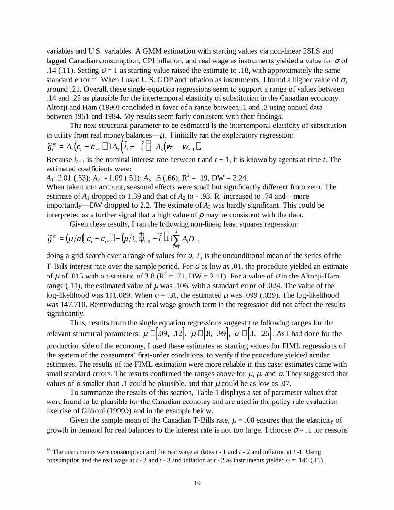
The next structural parameter to be estimated is the intertemporal elasticity of substitutionin utility from real money balances—µ. I initially ran the exploratory regression:

( ) ( ) ( )~ ~ ~g A A At

mt t t t t t= − + − + −− + −1 1 2 1 3 1c c i i w w .

Because it + 1 is the nominal interest rate between t and t + 1, it is known by agents at time t. Theestimated coefficients were:A1: 2.01 (.63);A2: - 1.09 (.51); A3: .6 (.66); R2 = .19, DW = 3.24.When taken into account, seasonal effects were small but significantly different from zero. Theestimate of A1 dropped to 1.39 and that of A2 to - .93. R2 increased to .74 and—moreimportantly—DW dropped to 2.2. The estimate of A3 was hardly significant. This could beinterpreted as a further signal that a high value of ρ may be consistent with the data.

Given these results, I ran the following non-linear least squares regression:

( )( ) ( )( ) ∑=

+− +−−−=4

1101

~~~i

iittttmt DAig iicc µσµ ,

doing a grid search over a range of values for σ. i 0 is the unconditional mean of the series of the

T-Bills interest rate over the sample period. For σ as low as .01, the procedure yielded an estimateof µ of .015 with a t-statistic of 3.8 (R2 = .71, DW = 2.11). For a value of σ in the Altonji-Hamrange (.11), the estimated value of µ was .106, with a standard error of .024. The value of thelog-likelihood was 151.089. When σ = .31, the estimated µ was .099 (.029). The log-likelihoodwas 147.710. Reintroducing the real wage growth term in the regression did not affect the resultssignificantly.

Thus, results from the single equation regressions suggest the following ranges for the

relevant structural parameters: [ ] [ ] [ ]µ ρ σ∈ ∈ ∈. , . , . , . , . , .09 12 8 99 1 25. As I had done for the

production side of the economy, I used these estimates as starting values for FIML regressions ofthe system of the consumers’ first-order conditions, to verify if the procedure yielded similarestimates. The results of the FIML estimation were more reliable in this case: estimates came withsmall standard errors. The results confirmed the ranges above for µ, ρ, and σ. They suggested thatvalues of σ smaller than .1 could be plausible, and that µ could be as low as .07.

To summarize the results of this section, Table 1 displays a set of parameter values thatwere found to be plausible for the Canadian economy and are used in the policy rule evaluationexercise of Ghironi (1999b) and in the example below.

Given the sample mean of the Canadian T-Bills rate, µ = .08 ensures that the elasticity ofgrowth in demand for real balances to the interest rate is not too large. I choose σ = .1 for reasons

36 The instruments were consumption and the real wage at dates t - 1 and t - 2 and inflation at t -1. Usingconsumption and the real wage at t - 2 and t - 3 and inflation at t - 2 as instruments yielded σ = .146 (.11).

20

of convergence of aggregate consumption to the steady state after a shock.37 In order to speed upconvergence, I actually set β = .95 rather than .99 in the calibration exercise. This change in thevalue of β does not affect the ranges of estimates of the other parameters in any significant wayand is useful for exposition purposes. ρ is probably a more controversial choice, though .8 seemsa sensible starting value.

4. A Recession in the United States

In this section, I illustrate the functioning of the model by analyzing the transmission of arecession in the U.S. to Canada under inflation targeting—the monetary regime currently followedby the Bank of Canada.

Shocks to U.S. variables cannot be taken in isolation. In Ghironi (1999a), I do not modelthe structure of the U.S. economy as explicitly as Canada’s but—at a minimum—one mustrecognize that four variables that appear in the equations for Canadian variables will be affectedby shocks to U.S. GDP or interest rate: besides these, the U.S. CPI inflation rate and the realinterest rate will change. Movements in U.S. inflation and interest rates will affect Canada throughPPP and interest rate parities. One cannot analyze the consequences of a shock to U.S. output orthe interest rate for Canada without explicitly accounting for the comovements in all relevantvariables that are triggered by the initial disturbance.

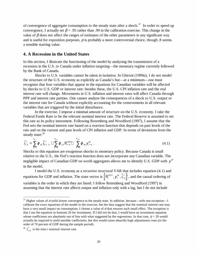
In the exercise, I impose a minimal amount of structure on the U.S. economy. I take theFederal Funds Rate to be the relevant nominal interest rate. The Federal Reserve is assumed to setthis rate as its policy instrument. Following Rotemberg and Woodford (1997), I assume that theFed sets the nominal interest rate based on a reaction function that depends on past levels of therate and on the current and past levels of CPI inflation and GDP. In terms of deviations from thesteady state:38

~ ~ ~* * *~* ~ *

i i yi y

t k t kk

n

k t kCPI

k

n

k t kW

k

n W

+ + −=

−=

−=

= + +∑ ∑ ∑1 1 11

20

30

ϕ ϕ π ϕπ

. (4.1)

Shocks to this equation are exogenous shocks to monetary policy. Because Canada is smallrelative to the U.S., the Fed’s reaction function does not incorporate any Canadian variable. Thenegligible impact of Canadian GDP on world aggregates allows me to identify U.S. GDP with y W

in the model.I model the U.S. economy as a recursive structural VAR that includes equation (4.1) and

equations for GDP and inflation. The state vector is [ ]~ , ,~

'* *π tCPI

tW

ty i +1 , and the causal ordering of

variables is the order in which they are listed. I follow Rotemberg and Woodford (1997) inassuming that the interest rate affects output and inflation only with a lag, but I do not include

37 Higher values of σ yield slower convergence to the steady state. In addition, because—with one exception—Icalibrate the exact equations of the model in the exercise, but the data suggest that the nominal interest rate mayhave a very small impact on consumption, I choose a value of σ that ensures such small effect. The exception isthat I use the equation in footnote 20 for investment. If I did not do that, I would have an investment equationwhose coefficients are absolutely out of line with what suggested by the regressions. In that case, η = 20 wouldactually be required to yield sensible coefficients, but this would cause absurdly high adjustments costs (in theorder of 70 percent of GDP during the sample period).38 i t +1

* is the time t nominal interest rate.

21

future inflation and GDP in the time-t state vector, because I do not believe that futureconsumption and inflation levels are entirely predetermined.

I estimate the VAR with three lags using full information maximum likelihood. I use databetween 1980:1 and 1997:4. The estimated coefficients for the three equations and the standarderrors are in the columns of Table 2. Seasonal dummies were not significant, as well as furtherlags. The estimated coefficients for the Fed’s reaction function suggest behavior in line with ageneralized Taylor rule, consistent with the findings of Rotemberg and Woodford (1997).

Figure 4 shows the responses of GDP, inflation, and the Federal Funds Rate to a 1%decrease in U.S. GDP. 39 40 The deviation of GDP from the steady state increases in the first twoquarters. Inflation reacts with a lag, and subsequently drops. The Fed reacts immediately bylowering the Federal Funds Rate to sustain GDP. 41 Over time, all variables go back to the steadystate.

The paths of U.S. variables generated by the shock constitute the paths of the exogenousworld-economy variables following the initial impulse in my model of the Canadian economy. Theestimated VAR equations are included in the system of equations that govern the dynamics of theworld economy following the initial shock, along with the model equations for Canada and themonetary rule followed by the Bank of Canada. The system is then solved using routines thatfollow Uhlig (1997).

The monetary rule followed by the Bank of Canada is perfectly neutral as far as the realinterest rate is concerned in all periods in which no shock happens. Under all rules the Canadianreal interest rate is equal to the U.S. real interest rate—except in the case of short-run deviationsfrom uncovered interest parity due to unexpected shocks. Different rules can make a differencefor the dynamics of the Canadian economy via real interest rate effects only in the very short run.However, alternative policy rules can produce different dynamics by causing differences in thebehavior of the relative price, ( )p i P , which can be taken as a measure of the terms of trade for

the Canadian economy.42

In this illustrative example, I focus on inflation targeting, the regime currently followed bythe Bank of Canada. Under this regime, I assume that the Bank of Canada sets the Canadiannominal interest rate to keep CPI inflation at its steady-state level in all periods, including whenan unexpected shock happens: ~π t

CPI t t= ∀ ≥0 0 .43 44

39 Because markets clear in the model, an exogenous decrease in U.S. GDP can be interpreted both as theconsequence of a generalized decline in world demand for goods and as the outcome of a negative supply shock. Iinterpret the shock as an exogenous contraction in demand. The interpretation is consistent with the fact that U.S.inflation declines following the disturbance.40 In the impulse responses, the level of the interest rate at each point in time is the value chosen by the monetaryauthority at that date.41 A measure of the U.S. real interest rate can be obtained by using the response of the inflation rate to deflate thatof the Federal Funds Rate. The real interest rate reacts with a lag. It falls below the steady state in the first quarterafter the shock and remains lower than its long-run level until it eventually returns to it.42 The terms of trade are actually given by ( ) ( )( )fpip *ε , where ( )p f* is the U.S. PPI. Under my

assumptions, the fraction of Canadian goods in the U.S. consumption bundle is negligible. Hence, ( )p f* is only

marginally different from P* . Because of purchasing power parity, ( ) ( ) ( ) PipPip =*ε .43 Svensson (1998) distinguishes between strict and flexible inflation targeting depending on the weights attachedto different targets in the policymaker’s loss function. In both cases, the central bank is minimizing a loss function

22

An operational rule that is consistent with this target can be obtained from the moneydemand equation. Inflation will be constant at its steady-state level in all periods if the Bank ofCanada sets its interest rate as:

( ) ( )( ) ( ) ( )[ ]( )101001 11~~~−−+ −−−−−+−= tttt

Mttt iii wwccgii σσρσµ .

Strict inflation targeting requires the Bank of Canada to raise its interest rate if it did so in theprevious period and if consumption is growing, and to lower it if money growth and/or the realwage are rising.45

Impulse responses under this rule are in Figure 5. The Canadian dollar depreciates afterthe initial period, consistent with the decline in U.S. inflation.46 The Bank of Canada lowers itsinterest rate by less than the Fed, which generates expectation of depreciation in the periodsfollowing the shock. PPI inflation falls slightly on impact, but climbs above the steady state byeven less within a year. The relative price of the representative Canadian good falls, and themarkup rises. According to the model, firms absorb part of the contractionary consequences ofthe shock by accepting a lower real price for their output. They preserve profitability by raisingthe markup component of the price level. Consistent with theory and data, the markup iscountercyclical. Labor demand falls, and so does the real wage, though both are above the steadystate six quarters after the shock. Tobin’s q rises. Firms invest and substitute capital for labor.47

This causes an initial increase in share price inflation, which is absorbed rapidly. GDP drops, but itbounces above the steady state in two years. The recession is not as pronounced as in the U.S.Consumption falls and, save for a brief recovery in the third and fourth quarters after the shock, itcontinues to fall for eight years. It goes back to the steady state only in the very long run.48

Money balances initially rise, but fall below the steady state in the third quarter. Canada runs afairly persistent current-account deficit.49

Schmitt-Grohé (1998) uses a VAR approach to study how shocks to U.S. GDP aretransmitted to the Canadian economy. She compares the predictions of the estimated VAR tothose of alternative flexible price models. She finds that the models can explain the observedresponses of output, hours, and capital only if larger-than-realistic movements in relative pricesare allowed. She raises the question of whether relaxing the assumption of price flexibility might

that attaches weight to inflation variability and interest-rate changes. Under flexible inflation targeting, thepolicymaker cares about output volatility too. In reality, the Bank of Canada has an interval target for CPIinflation.44 An important dimension of inflation targeting in the real world is the choice of the steady-state inflation rate,

i.e., the actual target, given by 0π in my model. When evaluating the consequences of inflation targeting, one

would want to discuss the implications of different levels of the target. My model is not appropriate to perform

such analysis. Because firms face costs of output price inflation volatility around 0π , the choice of the steady-state

level of inflation has no consequence for welfare in the economy, because it does not affect the steady-state level ofthe markup or the dynamics of relative prices.45 The latter as long as σ < 1.46 I use the word depreciation to refer to an increase of the rate of depreciation above its steady-state level. The rateof depreciation does not change on impact because U.S. inflation reacts with a lag.47 In the impulse responses, capital at each point in time is capital at the end of the corresponding period ratherthan at the beginning.48 Slow population growth motivates slow convergence of consumption to the steady state.49 The large deviation of the current account from the steady state should not alarm the reader. Because the steady-state current-account deficit in Canada is approximately .59% of GDP, the deficit never exceeds 5% of GDP in theexercise, remaining within entirely plausible limits.

23

help remove the puzzle. My exercise provides a positive answer to the question. The impulseresponses for output, hours, and capital in the example above are consistent with the size andduration of the recession in the U.S. At the same time, fairly small movements in the relative priceof Canadian goods and other variables are observed.

In Ghironi (1999b), I compare inflation targeting to several other rules, including a fixedexchange rate regime with the U.S. and the Taylor rule. I assume that Canada is subject to threesources of volatility: shocks to U.S. GDP, exogenous movements in U.S. monetary policy, andtechnology shocks. Welfare comparisons support the choice of a constant inflation rate as theoptimal monetary rule among those considered for the Canadian economy. Markup and relativeprice dynamics under that rule ensure the smallest volatility of consumption. Abandoning inflationtargeting for a fixed exchange rate regime with the U.S. would not be welfare improving,although the performance of the two regimes is fairly similar. A forward-looking version of theTaylor rule dominates the traditional version.

5. Conclusions

I have estimated the structural parameters of a small open economy model using data fromCanada and the United States. The model—presented in detail in Ghironi (1999a)—improvesupon the existing theoretical literature from an empirical perspective. I solve the stationarityproblem that characterizes several existing models by adopting an overlapping generationsstructure a’ la Weil (1989), in which new infinitely lived agents enter the economy at each point intime owning no assets. I model nominal rigidity explicitly, incorporating endogenous markupvariability, and I bring investment and capital accumulation into the analysis. The paper alsoillustrated a plausible strategy for constructing measures for unobservable variables. I estimatedthe parameters mainly by making use of non-linear least squares at the single equation level. I thenverified whether multiple-equation regressions yielded significantly different estimates by runningfull information maximum likelihood regressions based on the systems of the consumers’ first-order conditions and the firms’ first-order conditions. The approach was fairly successful. Non-linear least squares and full information maximum likelihood yielded fairly similar estimates. Mostparameter estimates were characterized by small standard errors and were in line with the findingsof other studies. Perhaps not surprisingly, given the use of aggregate data for the estimationprocedure, the size of the nominal rigidity and the size of the cost of adjusting the capital stockwere the only troublesome parameters. More work on these is to be done in the future.

In Section 4, I illustrated the functioning of the model by analyzing the transmission of arecession in the U.S. to Canada under inflation targeting, the monetary regime currently followedby the Bank of Canada. Consistent with the goal of combining theoretical rigor with an empiricalapproach, I used a simple VAR to trace the impact of comovements in U.S. variables on theCanadian economy. The estimated VAR equations for the U.S. were combined with the modelequations for Canada to determine the response of the Canadian economy to the initial shock. Theexample illustrated the role of markup and relative price dynamics in the model.

In Ghironi (1999b), I use the model and the parameter estimates to evaluate theperformance of alternative monetary rules for the Canadian economy. A constant path of inflationyields the smallest volatility of consumption and is thus the optimal rule among those I consider.The exercise provides interesting insights on the pros and cons of different rules, pointing to theimportance of transmission channels that are not featured in other studies of monetary rules for

24

open economies. The findings of this paper—which I see as an initial contribution to “new openeconomy macroeconometrics”—and of its companion suggest an empirical “case-by-case”approach as a profitable way to understand macroeconomic interdependence and address relevantpolicy issues.

References

Altonji, Joseph G., and John C. Ham (1990): “Intertemporal Substitution, Exogeneity, andSurprises: Estimating Life Cycle Models for Canada,” Canadian Journal of Economics 23: 1-43.

Benigno, Gianluca (1999): “Real Exchange Rate Persistence with Endogenous MonetaryPolicy,” unpublished manuscript, University of California, Berkeley.

Benigno, Pierpaolo (1999): “Optimal Monetary Policy in a Currency Area,” unpublishedmanuscript, Princeton University.

Bergin, Paul R. (1997): “Monetary Policy, Investment Dynamics, and the IntertemporalApproach to the Current Account,” unpublished manuscript, University of California, Davis.

Calvo, Guillermo A. (1982): “On the Microfoundations of Staggered Nominal Contracts:A First Approximation,” mimeo, Columbia University.

Carré, Martine, and Fabrice Collard (1997): “Asymmetric Shocks and Monetary Union,”unpublished manuscript, CREST-MAD Université de Paris I and CNRS-Cepremap.

Corsetti, Giancarlo, and Paolo Pesenti (1998): “Welfare and MacroeconomicInterdependence,” NBER Working Paper No. 6307.

Cushman, David O., and Tao Zha (1997): “Identifying Monetary Policy in a Small OpenEconomy under Flexible Exchange Rates,” Journal of Monetary Economics 39: 433-448.

Engel, Charles, and John H. Rogers (1996): “How Wide is the Border?,” AmericanEconomic Review 86: 1112-1125.

Gali, Jordi, and Tommaso Monacelli (1999): “Optimal Monetary Policy and ExchangeRate Volatility in a Small Open Economy,” unpublished manuscript, Department of Economics,Universitat Pompeu Fabra and New York University, and Department of Economics, BostonCollege.

Ghironi, Fabio (1999a): “Towards New Open Economy Macroeconometrics,”unpublished manuscript, International Research Function, Federal Reserve Bank of New York(available at http://home.earthlink.net/~ghiro/noeme.pdf).

Ghironi, Fabio (1999b): “Alternative Monetary Rules for a Small Open Economy: TheCase of Canada,” unpublished manuscript, International Research Function, Federal ReserveBank of New York (available at http://home.earthlink.net/~ghiro/canada.pdf).

Ghironi, Fabio (2000): “U.S.-Europe Economic Interdependence and PolicyTransmission,” unpublished manuscript, International Research Function, Federal Reserve Bankof New York (available at http://home.earthlink.net/~ghiro/eusa2.pdf).

Hall, Robert E. (1978): “Stochastic Implications of the Life Cycle-Permanent IncomeHypothesis: Theory and Evidence,” Journal of Political Economy 86 (December): 971-987.

Hayashi, Fumio (1982): “Tobin’s Marginal q and Average q: A NeoclassicalInterpretation,” Econometrica 50 (January): 213-224.

Hayashi, Fumio, and Tohru Inoue (1991): “The Relation between Firm Growth and q withMultiple Capital Goods: Theory and Evidence from Panel Data on Japanese Firms,”Econometrica 59 (May): 731-753.

25

Ireland, Peter (1997): “A Small, Structural, Quarterly Model for Monetary PolicyEvaluation,” Carnegie-Rochester Conference Series on Public Policy 47: 83-108.

Ireland, Peter (1999): “Sticky-Price Models of the Business Cycle: Specification andStability,” unpublished manuscript, Boston College.

Kollmann, Robert (1999): “Explaining International Comovements of Output and AssetReturns: The Role of Money and Nominal Rigidities,” IMF Working Paper 99/84.

Lane, Philip (1999): “The New Open Economy Macroeconomics: A Survey,” CEPRDiscussion Paper No. 2115.

Leeper, Eric M., Christopher A. Sims, and Tao Zha (1996): “What Does Monetary PolicyDo?,” Brookings Papers on Economic Activity 2: 2-63.

Mendoza, Enrique G. (1991): “Real Business Cycles in a Small Open Economy,”American Economic Review 81 (September): 797-818.

Obstfeld, Maurice, and Kenneth Rogoff (1995): “Exchange Rate Dynamics Redux,”Journal of Political Economy 103 (June): 624-60.

Obstfeld, Maurice, and Kenneth Rogoff (1996): “Foundations of InternationalMacroeconomics,” Cambridge: MIT Press.

Obstfeld, Maurice, and Kenneth Rogoff (1998): “Risk and Exchange Rates,” NBERWorking Paper No. 6694.

Obstfeld, Maurice, and Kenneth Rogoff (2000): “New Directions for Stochastic OpenEconomy Models,” Journal of International Economics 50: 117-153.

Ramey, Valerie A., and Kenneth D. West (1997): “Inventories,” NBER Working PaperNo. 6315.

Rotemberg, Julio J. (1982): “Monopolistic Price Adjustment and Aggregate Output,”Review of Economic Studies 49: 517-531.

Rotemberg, Julio J., and Michael Woodford (1990): “Cyclical Markups: Theories andEvidence,” NBER Working Paper No. 3534.

Rotemberg, Julio J., and Michael Woodford (1993): “Dynamic General EquilibriumModels with Imperfectly Competitive Product Markets,” NBER Working Paper No. 4502.

Rotemberg, Julio J., and Michael Woodford (1997): “An Optimization-BasedEconometric Framework for the Evaluation of Monetary Policy,” in Bernanke, Ben, and Julio J.Rotemberg (Eds.), NBER Macroeconomics Annual, 297-346.

Schaller, Huntley (1993): “Asymmetric Information, Liquidity Constraints, and CanadianInvestment,” Canadian Journal of Economics 26: 552-574.

Schmitt-Grohé, Stephanie (1998): “The International Transmission of EconomicFluctuations: Effects of U.S. Business Cycles on the Canadian Economy,” Journal ofInternational Economics 44: 257-287.

Smets, Frank, and Raf Wouters (1999): “The Exchange Rate and the MonetaryTransmission Mechanism in Germany,” De Economist, forthcoming.

Svensson, Lars E. O. (1998): “Open-Economy Inflation Targeting,” CEPR DiscussionPaper No. 1989.

Uhlig, Harald (1997): “A Toolkit for Analyzing Nonlinear Dynamic Stochastic ModelsEasily,” unpublished manuscript, CentER, University of Tilburg.

Weil, Philippe (1989): “Overlapping Families of Infinitely-Lived Agents,” Journal ofPublic Economics 38 (March): 183-198.

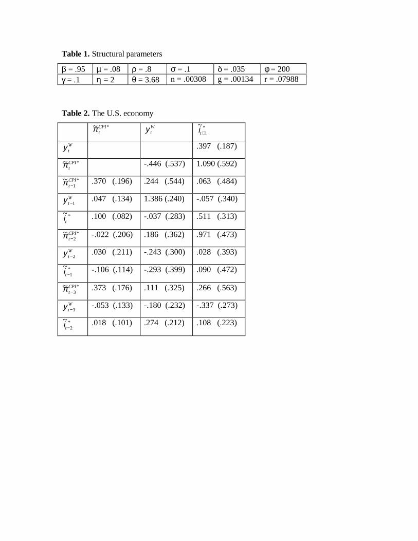
Table 1. Structural parameters

β = .95 µ = .08 ρ = .8 σ = .1 δ = .035 φ = 200γ = .1 η = 2 θ = 3.68 n = .00308 g = .00134 r = .07988

Table 2. The U.S. economy

~ *π tCPI y t

W ~*it +1

y tW .397 (.187)

~ *π tCPI -.446 (.537) 1.090 (.592)

~ *π tCPI−1

.370 (.196) .244 (.544) .063 (.484)

y tW−1

.047 (.134) 1.386 (.240) -.057 (.340)

~*it .100 (.082) -.037 (.283) .511 (.313)

~ *π tCPI−2

-.022 (.206) .186 (.362) .971 (.473)

y tW−2

.030 (.211) -.243 (.300) .028 (.393)

~*it −1-.106 (.114) -.293 (.399) .090 (.472)

~ *π tCPI−3

.373 (.176) .111 (.325) .266 (.563)

y tW−3

-.053 (.133) -.180 (.232) -.337 (.273)

~*it −2.018 (.101) .274 (.212) .108 (.223)

Figure 1. Markup and hours

-0.1

-0.08

-0.06

-0.04

-0.02

0

0.02

0.04

0.06

0.08

0.1

0.12

1980

Q2

1980

Q4

1981

Q2

1981

Q4

1982

Q2

1982

Q4

1983

Q2

1983

Q4

1984

Q2

1984

Q4

1985

Q2

1985

Q4

1986

Q2

1986

Q4

1987

Q2

1987

Q4

1988

Q2

1988

Q4

1989

Q2

1989

Q4

1990

Q2

1990

Q4

1991

Q2

1991

Q4

1992

Q2

1992

Q4

1993

Q2

1993

Q4

1994

Q2

1994

Q4

1995

Q2

1995

Q4

1996

Q2

1996

Q4

1997

Q2

1997

Q4

gMarkup gHours

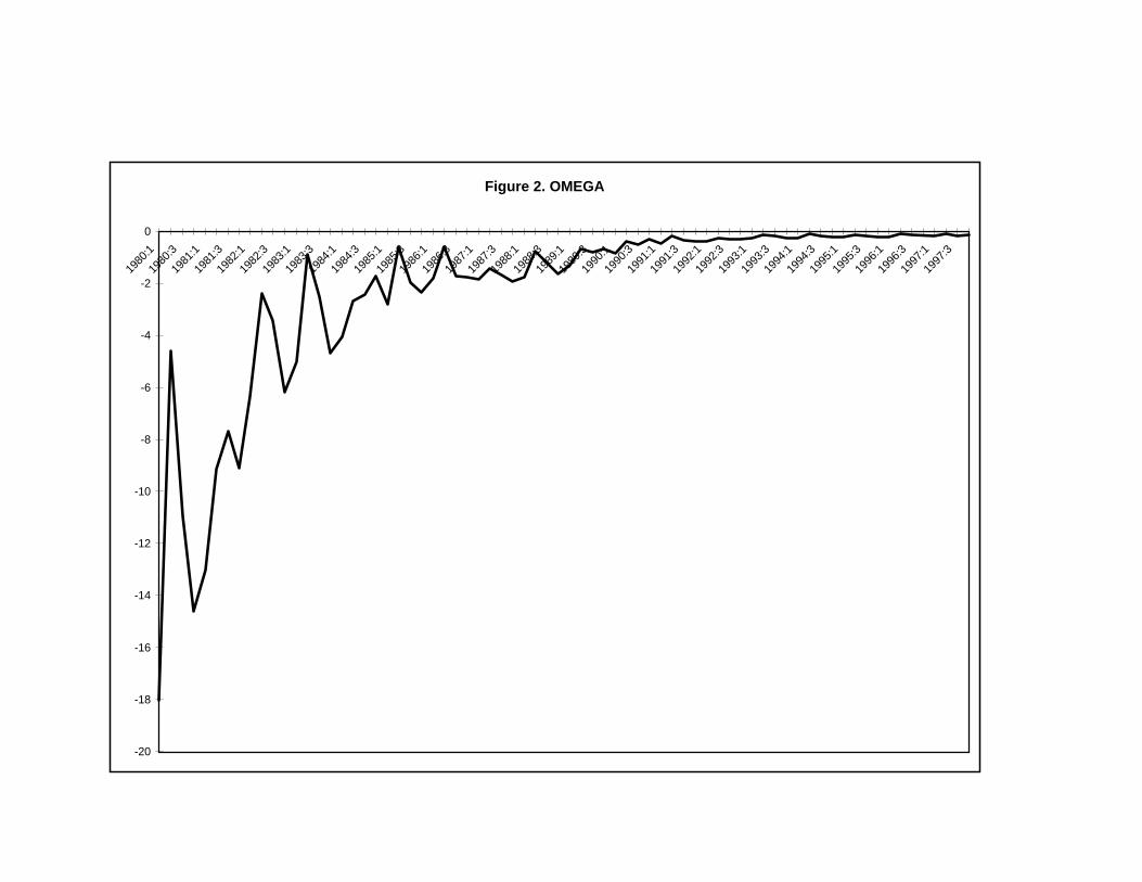
Figure 2. OMEGA

-20

-18

-16

-14

-12

-10

-8

-6

-4

-2

0

1980

:119

80:3

1981

:119

81:3

1982

:119

82:3

1983

:119

83:3

1984

:119

84:3

1985

:119

85:3

1986

:119

86:3

1987

:119

87:3

1988

:119

88:3

1989

:119

89:3

1990

:119

90:3

1991

:119

91:3

1992

:119

92:3

1993

:119

93:3

1994

:119

94:3

1995

:119

95:3

1996

:119

96:3

1997

:119

97:3

Figure 3.a. Investment and average q

30

35

40

45

50

55

60

1980

Q1

1980

Q3

1981

Q1

1981

Q3

1982

Q1

1982

Q3

1983

Q1

1983

Q3

1984

Q1

1984

Q3

1985

Q1

1985

Q3

1986

Q1

1986

Q3

1987

Q1

1987

Q3

1988

Q1

1988

Q3

1989

Q1

1989

Q3

1990

Q1

1990

Q3

1991

Q1

1991

Q3

1992

Q1

1992

Q3

1993

Q1

1993

Q3

1994

Q1

1994

Q3

1995

Q1

1995

Q3

1996

Q1

1996

Q3

1997

Q1

1997

Q3

0.88

0.93

0.98

1.03

1.08

1.13

investment average q

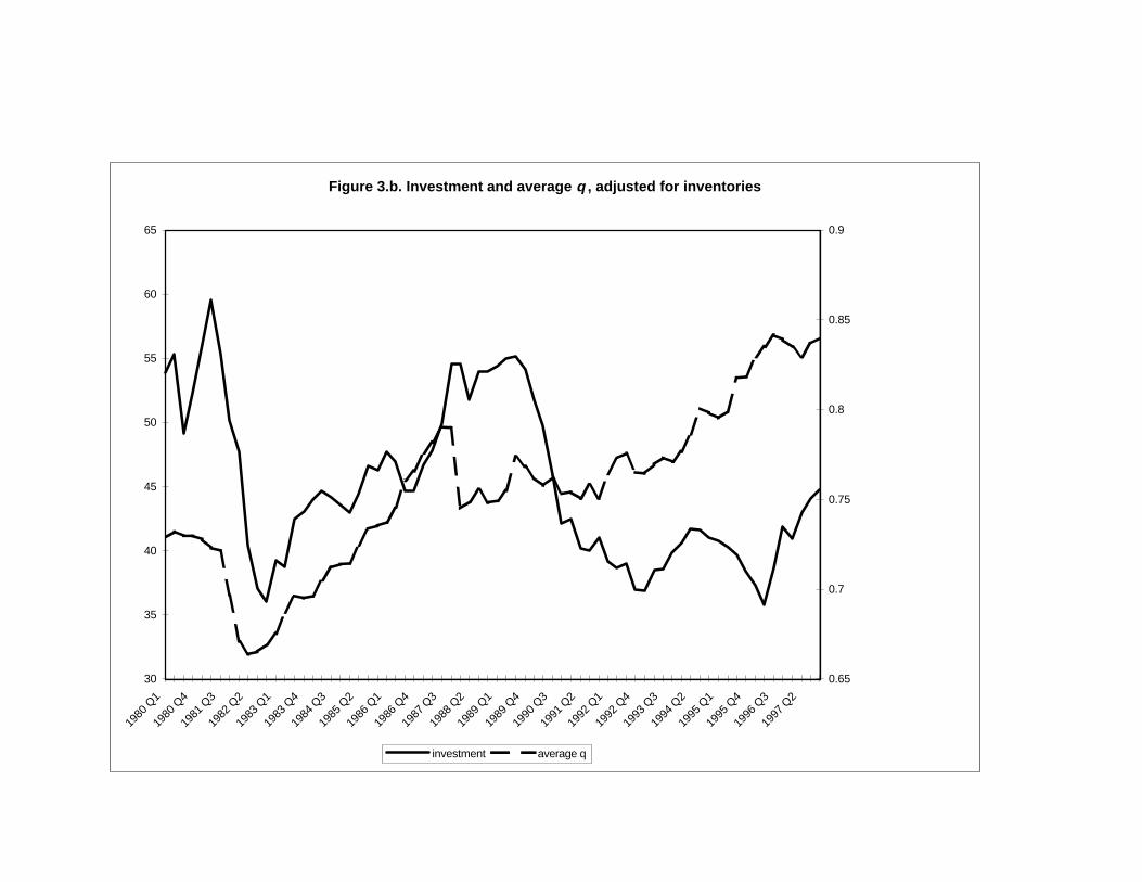
Figure 3.b. Investment and average q , adjusted for inventories

30

35

40

45

50

55

60

65

1980

Q1

1980

Q4

1981

Q3

1982

Q2

1983

Q1

1983

Q4

1984

Q3

1985

Q2

1986

Q1

1986

Q4

1987

Q3

1988

Q2

1989

Q1

1989

Q4

1990

Q3

1991

Q2

1992

Q1

1992

Q4

1993

Q3

1994

Q2

1995

Q1

1995

Q4

1996

Q3

1997

Q2

0.65

0.7

0.75

0.8

0.85

0.9

investment average q

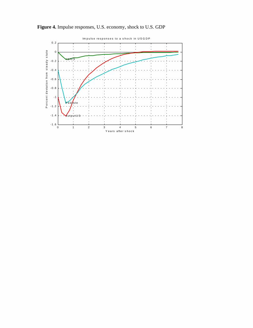
Figure 4. Impulse responses, U.S. economy, shock to U.S. GDP

0 1 2 3 4 5 6 7 8-1 .6

-1 .4

-1 .2

-1

-0 .8

-0 .6

-0 .4

-0 .2

0

0 . 2

Im p u ls e re s p o n s e s t o a s h o c k in U S G D P

Y e a rs a fte r s h o c k

Pe

rce

nt

de

via

tio

n f

rom

ste

ad

y s

tate

c p iU S

o u t p u t U S

F e d ra t e

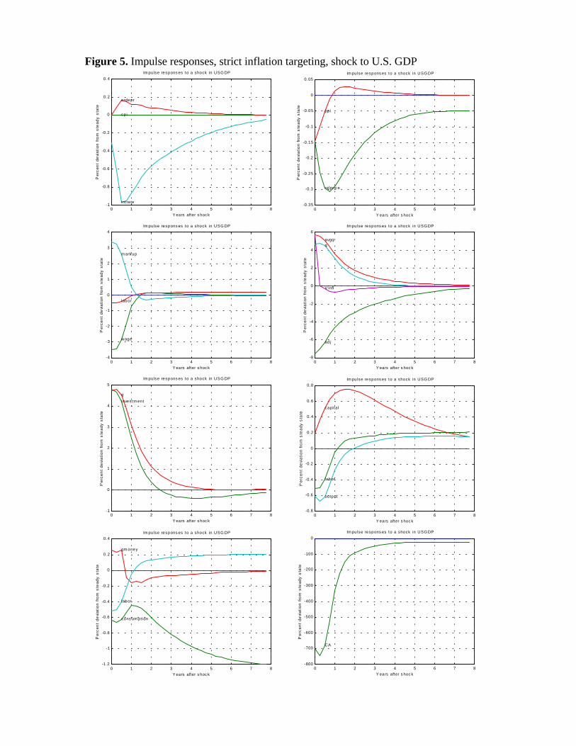
Figure 5. Impulse responses, strict inflation targeting, shock to U.S. GDP

0 1 2 3 4 5 6 7 8-1

-0.8

-0.6

-0.4

-0.2

0

0.2

0.4

Im pulse respons es to a shock in USG DP

Y ears after s hoc k

Pe

rce

nt

de

via

tio

n f

rom

ste

ad

y s

tate

cp i

erdepr

int ra te

0 1 2 3 4 5 6 7 8-0.35

-0.3

-0.25

-0.2

-0.15

-0.1

-0.05

0

0.05Im pulse respons es to a shock in USG DP

Y ears after s hoc k

Pe

rce

nt

de

via

tio

n f

rom

ste

ad

y s

tate

relprice

pp i

0 1 2 3 4 5 6 7 8-4

-3

-2

-1

0

1

2

3

4Im pulse respons es to a shock in USG DP

Y ears after s hoc k

Pe

rce

nt

de

via

tio

n f

rom

ste

ad

y s

tate

wage

labor

m arkup

0 1 2 3 4 5 6 7 8-8

-6

-4

-2

0

2

4

6Im pulse respons es to a shock in USG DP

Y ears after s hoc k

Pe

rce

nt

de

via

tio

n f

rom

ste

ad

y s

tate

ad j

avgq q

V infl

0 1 2 3 4 5 6 7 8-1

0

1

2

3

4

5

Im pulse respons es to a shock in USG DP

Y ears after s hoc k

Pe

rce

nt

de

via

tio

n f

rom

ste

ad

y s

tate

investm ent

q

0 1 2 3 4 5 6 7 8-0.8

-0.6

-0.4

-0.2

0

0.2

0.4

0.6

0.8Im pulse respons es to a shock in USG DP

Y ears after s hoc k

Pe

rce

nt

de

via

tio

n f

rom

ste

ad

y s

tate

labor

capital

output

0 1 2 3 4 5 6 7 8-1.2

-1

-0.8

-0.6

-0.4

-0.2

0

0.2

0.4Im pulse respons es to a shock in USG DP

Y ears after s hoc k

Pe

rce

nt

de

via

tio

n f

rom

ste

ad

y s

tate

cons um pt ion

gm oney

labor

0 1 2 3 4 5 6 7 8-800

-700

-600

-500

-400

-300

-200

-100

0

Im pulse respons es to a shock in USG DP

Y ears after s hoc k

Pe

rce

nt

de

via

tio

n f

rom

ste

ad

y s

tate

CA