Towards Metamerism via Foveated S Transfer

Published as a conference paper at ICLR 2019

TowardsMetamerism via Foveated Style Transfer

Arturo Deza1,4, Aditya Jonnalagadda3, Miguel P. Eckstein1,2,4

1 Dynamical Neuroscience, 2Psychological and Brain Sciences,3Electric and Computer Engineering, 4 Institute for Collaborative BiotechnologiesUC Santa Barbara, CA, [email protected],[email protected],[email protected]

Abstract

The problem of visual metamerism is defined as finding a family of perceptuallyindistinguishable, yet physically different images. In this paper, we propose ourNeuroFovea metamer model, a foveated generative model that is based on a mixtureof peripheral representations and style transfer forward-pass algorithms. Ourgradient-descent free model is parametrized by a foveated VGG19 encoder-decoderwhich allows us to encode images in high dimensional space and interpolatebetween the content and texture information with adaptive instance normalizationanywhere in the visual field. Our contributions include: 1) A framework forcomputing metamers that resembles a noisy communication system via a foveatedfeed-forward encoder-decoder network – We observe that metamerism arises as abyproduct of noisy perturbations that partially lie in the perceptual null space; 2)A perceptual optimization scheme as a solution to the hyperparametric nature ofour metamer model that requires tuning of the image-texture tradeoff coefficientseverywhere in the visual field which are a consequence of internal noise; 3) AnABX psychophysical evaluation of our metamers where we also find that the rateof growth of the receptive fields in our model match V1 for reference metamers andV2 between synthesized samples. Our model also renders metamers at roughly asecond, presenting a ×1000 speed-up compared to the previous work, which allowsfor tractable data-driven metamer experiments.

1 IntroductionThe history of metamers originally started through color matching theory, where two light sourceswere used to match a test light’s wavelength, until both light sources are indistinguishable from eachother producing what is called a color metamer. This leads to the definition of visual metamerism:when two physically different stimuli produce the same perceptual response (See Figure 1 for anexample). Motivated by Balas et al. (2009)’s work of local texture matching in the periphery as amechanism that explains visual crowding, Freeman & Simoncelli (2011) were the first to create suchpoint-of-fixation driven metamers through such local texture matching models that tile the entirevisual field given log-polar pooling regions that simulate the V1 and V2 receptive field sizes, as wellas having global image statistics that match the metamer with the original image. The essence oftheir algorithm is to use gradient descent to match the local texture (Portilla & Simoncelli (2000))and image statistics of the original image throughout the visual field given a point of fixation untilconvergence thus producing two images that are perceptually indistinguishable to each other.

However, metamerism research currently faces 2 main limitations: The first is that metamer renderingfaces no unique solution. Consider the potentially trivial examples of having an image I and itsmetamer M where all pixel values are identical except for one which is set to zero (making thisdifference unnoticeable), or the case where the metameric response arises from an imperceptible equalperturbation across all pixels as suggested in Johnson et al. (2016); Freeman & Simoncelli (2011).This is a concept similar to Just Noticeable Differences (Lubin (1997); Daly (1992)). However, likethe work of Freeman & Simoncelli (2011); Keshvari & Rosenholtz (2016); Rosenholtz et al. (2012);Balas et al. (2009), we are interested in creating point-of-fixation driven metamers, which createimages that preserve information in the fovea, yet lose spatial information in the periphery such thatthis loss is unnoticeable contingent of a point of fixation (Figure 1). The second issue is that thecurrent state of the art for a full field of view rendering of a 512px×512px metamer takes 6 hours fora grayscale image and roughly a day for a color image. This computational constraint makes data-

1


MetamerImage

Same or Different?

Figure 1: Two visual metamers are physically different images that when fixated on the orange dot(center), should remain perceptually indistinguishable to each other for an observer. Colored circleshighlight different distortions in the visual field that observers do not perceive in our model.

driven experiments intractable if they require thousands of metamers. From a practical perspective,creating metamers that are quick to compute may lead to computational efficiency in rendering ofVR foveated displays and creation of novel neuroscience experiments that require metameric stimulisuch as gaze-contingent displays, or metameric videos for fMRI, EEG, or Eye-Tracking.

We think there is a way to capitalize metamer understanding and rendering given the developmentsmade in the field of style transfer. We know that the original model of Freeman & Simoncelli (2011)consists of a local texture matching procedure for multiple pooling regions in the visual field as wellas global image content matching. If we can find a way to perform localized style transfer withproper texture statistics for all the pooling regions in the visual field, and if the metamerism viatexture-matching hypothesis is correct – we can in theory successfully render a metamer.

Within the context of style transfer, we would want a complete and flexible framework where asingle network can encode any style (or texture) without the need to re-train, and with the power ofproducing style transfer with a single forward pass, thus enabling real-time applications. Furthermore,we would want such framework to also control for spatial and scale factors (Gatys et al. (2017)) toenable foveated pooling (Akbas & Eckstein (2017); Deza & Eckstein (2016)) which is critical inmetamer rendering. The very recent work of Huang & Belongie (2017), provides such frameworkthrough adaptive instance normalization (AdaIN), where the content image is stylized by adjustingthe mean and standard deviation of the channel activations of the encoded representation to matchwith the style. They achieve results that rival those of Ulyanov et al. (2016); Johnson et al. (2016),with the added benefit of not being limited to a single texture in a feed-forward pipeline.

In our model: we stack a peripheral architecture on top of a VGGNet (Simonyan & Zisserman (2015))in its encoded feature space, to map an image into a perceptual space. We then add internal noise inthe encoded space of our model as a characterization that perceptual systems are noisy. We find thatinverting such modified image representation via a decoder results in a metamer. This breaks downour model into a foveated feed-forward ‘auto’ style transfer network, where the input image plays therole both of the content and the style, and internal network noise (stylized with the content statistics)serves as a proxy for intrinsic image texture. While our model uses AdaIN for style transfer and aVGGNet for texture statistics, our pipeline is extendible to other models that successfully executestyle transfer and capture proper texture statistics (Ustyuzhaninov et al. (2017)).

2 Design of the NeuroFovea modelTo construct our metamer we propose the following statement: A metamer M can be rendered bytransferring k localized styles over a content image I, controlled by a set of style-to-content ratios αifor every pooling region (i-th receptive field). More formally, our goal is to find a Metamer functionM(◦) : I → M, where an input image I ∈ RL is fed through a VGG-Net encoder E(·) : RL → RD

which is both the content and the style image, to produce the content feature C ∈ RD, where C = E(I)as shown in Figure 2. Let L = C ×H ×W, and D = C′ ×H′ ×W′ where {C,C′}, {H,H′}, {W,W′} arethe image/layer channels, height, width given the convolutional structure of the encoder (we dropfully connected layers). A noise patch colored via ZCA (Bell & Sejnowski (1995)) to match the

2


Noise

Image PeripheralArchitecture

VGG-NetEncoder

VGG-NetEncoder AdaIN

+VGG-NetDecoder

For every -th Pooling Region

NeuroFoveaMetamer

Meta VGG-Net Decoder

pix

2p

ix R

efinem

en

t

Figure 2: The NeuroFovea metamer generation schematic: An input image and a noise patch arefed through a VGG-Net encoder into a new feature space. Through spatial control we can producean interpolation for each pooling region in such feature space between the stylized-noise (texture),and the content (the input image). This is how we successfully impose both global image andlocal texture-like constraints in every pooling region. The metamer is the output of the pooled (andinterpolated) feature vector through the Meta VGG-Net Decoder.

content image’s mean and varianceN ∼ (µI ,σ2I ) ∈ RL is also fed through the same VGG-Net encoder

producing the noise feature N ∈ RD, where N = E(N). This is the internal perceptual noise of thesystem which will later on serve us as a proxy for texture encoding. These vectors are masked throughspatial control a la Gatys et al. (2017), and the noise is stylized via S(·) : RD→ RD with the contentwhich encodes the texture representation of the content in the feature space through Adaptive InstanceNormalization (AdaIN). A target feature Ti ∈ R

D is defined as an interpolation between the stylizednoise S(Ni) and the content Ci modulated by α, in the feature space RD for every i-th pooling region:

Ti(I|N ;α) = (1−α)Ci(I) +αS(Ni) (1)

In other words, in our quest to probe for metamerism, we are finding an intermediate representation(the convex combination) between two vectors representing the image and its texturized version (thestylized noise) in RD per pooling region as seen in Figure 3. Within the framework of style transfer,we could think of this as a content-vs-style or structure-vs-texture tradeoff, since the style and thecontent image are the same. Similar interpolations have been explored in Hénaff & Simoncelli (2016)via a joint pixel and network space minimization. The final target feature vector T is the maskedsum of every Ti with spatial control masks wi s.t. T =

∑wiTi. The metamer is the output of the

Meta VGG-Net decoder D(·) on T, where the decoder receives only one vector (T) and producesa global decoded output. Our Meta VGG-Net Decoder compensates for small artifacts by stackinga pix2pix Isola et al. (2017) U-Net refinement module which was trained on the Encoder-Decoderoutputs to map to the original high resolution image. Figure 2 fully describes our model, and themetamer transform is computed via:

M(I|N ; α) =D(E∑(I|N ; α)) =D(k∑

i=1

wi[(1−αi)Ei(I) +αiS(Ei(N))

]) (2)

where E∑ is the foveated encoder that is defined as the sum of encoder outputs over all the k poolingregions (our spatial controls masks wi) in the visual field. Note that the decoder was not trainedto generate metamers, but rather to invert the encoded image and act as E−1. It happens to be the

Figure 3: Interpolating between an image’s intrinsic content and texture via a convex combination inthe output of the VGG19 Encoder E. Here we are treating the patch as a single pooling region. In ourmodel, this interpolation given Eq. 1 is done for every pooling region in the visual field.

3


case that perturbing the encoded representation in the direction of the stylized noise by an amountspecified by the size of the pooling regions, outputs a metamer. Additional specifications and trainingof our model can be seen in the Supplementary Material.

2.1 Model Interpretability

Within the framework of metamerism where distortions lie on the perceptual null space as proposedinitially in color matching theory, and also in Freeman & Simoncelli (2011) for images, we can thinkof our model as a direct transform that is maximizing how much information to discard depending onthe texture-like properties of the image and the size of the receptive fields. Consider the following: ifour interpolation is projected from the encoded space to the perceptual space via P, from Eq. 1 weget PTi = P(1−α)Ci(I) + P(α)S(Ni), it follows that for each receptive field:

P Ti︸︷︷︸metamer

= P Ci︸︷︷︸image

+Pα(S⊥(Ni) +S‖(Ni))︸︷︷︸distortion

(3)

by decomposing S(Ni)−Ci = S⊥(Ni) +S‖(Ni), where S‖ is the projection of the difference vector onthe perceptual space, and S⊥(Ni) is the orthogonal component perpendicular to such vector which liesin the perceptual null space (PS⊥(Ni) = ~0). The value of these components will change dependingon the location of Ci and S(Ni), and the geometry of the encoded space. If ||S‖(Ni)||22 < ε, (i.e. theimage patch has strong texture-like properties), then α can vary above its critical value given thatS⊥(Ni) is in the null space of P and the distortion term will still be small; but if ||S‖(Ni)||22 > ε,α can not exceed its critical value for the metamerism condition to hold (PTi ≈ PCi). Thus ourinterest is in computing the maximal average amount of distortion (driven by α) given humansensitivity before observers can tell the difference. This is illustrated in Figure 4 via the bluecircle around Ci in the perceptual space which shows the metameric boundary for any distortion.

Encoded Space

Perceptual Space

Figure 4: Perceptual Projection.

One can also see the resemblance of the model to a noisy com-munication system in the context of information theory. Theinformation source is the image I, the transmitter and the re-ceiver are the encoder and decoders (E,D) respectively, and thenoise source is the encoded noise patch E(N) imposing texturedistortions in the visual field, and the destination is the metamerM. Highlighting this equivalence is important as metamerismcan also be explored within the context of image compressionand rate-distortion theory as in Ballé et al. (2017). Such ap-proaches are beyond the scope of this paper, however theyare worth exploring in future work as most metamer modelspurely involve texture and image analysis-synthesis matchingparadigms that are gradient-descent based.

3 Hyperparameteric nature of our modelSimilar to our model, the Freeman & Simoncelli (2011) model(hereto be abbreviated FS) requires a scale parameter s whichcontrols the rate of growth of the receptive fields as a function of eccentricity. This parameter shouldbe maximized such that an upperbound for perceptual discrimination is found. Given that textureand image matching occurs in each one of the pooling regions: a high scaling factor will likely makethe image rapidly distinguishable from the original as distortions are more apparent in the periphery.Conversely, a low scaling factor might gaurantee metamerism even if the texture statistics are not fullycorrect given that smaller pooling regions will simulate weak effects of crowding. Low scaling factorsin that sense are potentially uninteresting – it is the value up until humans can tell the differencethat is critical (Lubin (1997)). FS set out to find such critical value via a psychophysical experimentwhere they perform the following single-variable optimization to find such upper bound:

s0 = argmaxs

E[d′(s|θobs)] (4)

s.t. 0 < d′(s|θobs) < ε, where d′ = Φ−1(HR)−Φ−1(FA) is the index of detectability for each observerθobs, Φ is the cumulative of the gaussian distribution, and HR and FA are the hit rate and false alarmrates as defined in Green & Swets (1966). However, our model is different in regards to a set of

4


s = 0.25 s=0.50 s=0.75 s=1.0

Figure 5: Potential issues of psychophysical intractability for the joint estimation of (s) and γ(·) asdescribed by our model. Running a psychophysical experiment that runs an exhaustive search forupper bounds for the scale and distortion parameters for every receptive field is intractable. The goalof Experiment 1 is to solve this intractabitilty posed formally in Eq. 6 via a simulated experiment.

hyperparameters α that we must estimate everywhere in the visual field as summarized by the γfunction, where we assume α to be tangentially isotropic:

α = γ(◦; s) (5)

where each α represents the maximum amount of distortion (Eq. 1) that is allowed for every receptivefield in the visual periphery before an observer will notice. At a first glance, it is not trivial to know ifα should be a function of scale, retinal eccentricity, receptive field size, image content or potentially acombination of the before-mentioned (hence the ◦ in the γ function’s argument).

Thus, the motivation of α seems uncertain and perhaps un-necessary from the Occam’s razor per-spective of model simplicity. This raises the question: Why does the FS model not require anyadditional hyperparameters, requiring only a single scale (s) parameter? The answer lies in the natureof their model which is gradient descent based and where local texture statistics are matched for everypooling region in the visual field, while preserving global image structural information. When suchcondition is reached, no further synthesis steps are required as it is an equilibrium point. Indeed, theexperiments of Wallis et al. (2016) have shown that images do not remain metameric if the structuralinformation of a pooling region is discarded while purely retaining the texture statistics of Portilla& Simoncelli (2000). This motivates the purpose of α where we interpolate between structural andtexture representation. Thus our goal is to find that equilibirum point in one-shot, given that ourmodel is purely feed-forward and requires no gradient-descent (Eq. 2). At the expense of this artifice,we run into the challenge of facing a multi-variable optimization problem that has the risk of beingpsychophysically intractable. Analogous to FS, we must solve:

s0, α0 = argmaxs,α

E[d′(s, α|θobs)] (6)

s.t. 0 < d′(s, α|θobs) < ε. Figure 5 shows the potential intractability: each observer would have torun multiple rounds of an ABX experiment for a collection of many scales and α values for eachlocation in the visual field. Consider: (S scales) × (k pooling regions) × (αm step size for each α) ×(N images) × (w trials): S kNαmw trials per observer.

We will show in Experiment 1 that one solution to Eq. 6 is to find a relationship between each set ofα’s and the scale, expressed via the γ function. This requires a two stage process: 1) Showing thatsuch γ exists; 2) Estimate γ given s. If this is achieved, we can relax the multi-variable optimizationinto a single variable optimization problem, where 0 < d′(s,γ(◦; s)|θobs) < ε, and:

s0 = argmaxs

E[d′(s,γ(◦; s)|θobs)] (7)

4 ExperimentsThe goal of Experiment 1 is to estimate γ as a function of s via a computational simulation as a proxyfor running human psychophysics. Once it is computed, we have reduced our minimization to atractable single variable optimization problem. We will then proceed to Experiment 2 where we willperform an ABX experiment on human observers by varying the scale to render visual metamers asoriginally proposed by FS. We will use the images shown in Figure 6 for both our experiments.

5


Figure 6: A color-coded collection of images used in our experiments.

4.1 Experiment 1: Estimation of model hyperparameters via perceptual optimization

Existence and shape of γ: Given some biological priors, we would like γ to satisfy these properties:

1. γ : Z→ α s.t. Z ∈ [0,∞),α ⊂ [0,1), where z ∈ Z is parametrized by the size (radius) of eachreceptive field (pooling region) which grows with eccentricity in humans.

2. γ is continuous and monotonically non-decreasing since more information should not begained given larger crowding effects as receptive field size increases in the periphery.

3. γ has a unique zero at γ(0) = 0. Under ideal assumptions there is no loss of information inthe fovea, where the size of the receptive fields asymptotes to zero.

Indeed, we found that γ is sigmoidal, and is a function of z, parametrized by s:

γ(z; s) = a +b

c + exp(−dz)= −1 +

21 + exp(−d(s)z)

(8)

Figure 7: Perceptual optimization.

Estimation of γ: To numerically estimate theamount of α-noise distortion for each receptivefield in our metamer model we need to find away to simulate the perceptual loss made by ahuman observer when trying to discriminate be-tween metamers and original images. We willdefine a perceptual loss L that has the goal ofmatching the distortions via SSIM of a gradientdescent based method such as the FS metamers,and the NeuroFovea metamers (NF) with theirreference images – a strategy similar to Laparraet al. (2017) used for perceptual rendering. Wechose SSIM as it is a standard IQA metric thatis monotonic with human judgements, althoughother metrics such as MS-SSIM and IW-SSIMshow similar tuning properties for γ as shownin the Supplementary Material. Indeed the refer-ence image I′ for the NF metamer is limited bythe autoencoder-like nature of the model wherethe bottleneck usually limits perfect reconstruc-tion s.t. I′ = D(E(I))|(α=0), where I′ → I, andthey are only equal if the encoder-decoder pair(E,D) allows for lossless compression. Since we can not define a direct loss function L between themetamers, we will need their reference images to define a convex surrogate loss function LR. Thegoal of this function should be to match the perceptual loss of both metamers for each receptive field

6


1.0

0.8

0.6

0.4

0.2

0.0

0.30

0.25

0.20

0.15

0.10

0.00

0.05

1st Eccentricity R.F.

0.0 0.2 0.4 0.6 0.8 1.0

2nd Eccentricity R.F.

0.0 0.2 0.4 0.6 0.8 1.0

3rd Eccentricity R.F.

0.0 0.2 0.4 0.6 0.8 1.0

4th Eccentricity R.F.

0.0 0.2 0.4 0.6 0.8 1.0

Figure 8: The result of each SSIM (top) for Experiment 1 for a scale of s = 0.3 where we findthe critical α for each receptive field ring as we minimize E(∆-SSIM)2 (bottom). E(∆-SSIM)2 isminimized by matching the perceptual distortion of the Freeman & Simoncelli (2011) (MFS ) andNeuroFovea (MNF) metamers in Eq. 9. Each color represents a different 512×512 image trajectory,the black line (bottom) shows the average. Only the first 4 eccentricity dependent receptive fields areshown.

k when compared to their reference images: the original image I for the FS model, and the decodedimage I′ for the NF model:

LR(α|k) = E(∆-SSIM)2 =1N

N∑j=1

(SSIM(M( j,k)FS , I( j,k))−SSIM(M( j,k)

NF (γs), I′( j,k)))2 (9)

and αi should be minimized for each k pooling region via: α0 = argminαLR(α|k) for the collectionof N images. The intuition behind this procedure is shown in Figure 7. Note that if I′ = I, i.e. there isperfect lossless compression and reconstruction given the choice of encoder and decoder, then theoptimization is performed with reference to the same original image. This is an important observationas the reconstruction capacity of our decoder is limited despite E(MS-SSIM(I, I′) = 0.86±0.04. Onlyusing the original image in the optimization yields poor local minima at α = 0. Despite such limitation,we show that reference metamers can still be achieved for our lossy compression model.

Results: A collection of 10 images were used in our experiments. We then computed the SSIMscore for each FS and NF image paired with their reference image across each receptive field (R.F.)and averaged those that belonged to the same retinal eccentricity. Figure 8 (top) shows these results,as well as the convex nature of the loss function displayed in the bottom. This procedure wasrepeated for all the eccentricity-dependent receptive fields for a collection of 5 values of scale:{0.3,0.4,0.5,0.6,0.7}. A sigmoid to estimate γ was then fitted to each α per R.F. parametrized byscale via least squares. This gave us a collection of d values that control the slope rate of the sigmoid(Eq. 8). These were d : {1.240,1.196,1.363,1.311,1.355} respectively per scale, and {d} = 1.281 forthe ensemble of all scales. We then conducted a 10000 sample permutation test between the pairof (zs,αs) points per scale and the ensemble of points across all scales ({z}, {α}) that verified thattheir variation is statistically non-significant (p ≥ 0.05). Figure 9 illustrates the results from suchprocedure. We can conclude that the parameters of γ do not vary as we vary scale. In other words,the α = γ(z) function is fixed, and the scale parameter itself which controls receptive field size willimplicitly modulate the maximum α-noise distortion with a unique γ function. If the scale factor issmall, the maximum noise distortion in the far periphery will be small and vice versa if the scale islarge. We should point out that Figure 9 might suggest that the maximal noise distortion is contingenton image content as the scores are not uniform tangentially for the receptive fields that lie on the sameeccentricity ring. Indeed, we did simplify our model by computing an average and fitting the sigmoid.However, computing an average should approximate the maximal distortion for the receptive fieldsize on that eccentricity in the perceptual space for the human observer i.e. the metameric boundary.We elaborate more on this idea in the discussion section.

7


scale=0.3 scale=0.4 scale=0.5 scale=0.6 scale=0.7

1.0

0.8

0.6

0.4

0.2

0.0

Radius of R.F. (d.v.a.)0.0 0.5 1.0 1.5 2.0 2.5 3.0

Radius of R.F. (d.v.a.)0.0 0.5 1.0 1.5 2.0 2.5 3.0

Radius of R.F. (d.v.a.)0.0 0.5 1.0 1.5 2.0 2.5 3.0

Radius of R.F. (d.v.a.)0.0 0.5 1.0 1.5 2.0 2.5 3.0

Radius of R.F. (d.v.a.)0.0 0.5 1.0 1.5 2.0 2.5 3.0

1.0

0.8

0.6

0.4

0.2

0.0

d=1.240 d=1.196 d=1.363 d=1.311 d=1.355

Figure 9: Top: The average α-noise distortion over the entire visual field for our 10 images withoutassuming tangential homogeneity. Notice that on average, α increases radially. Bottom: The γ(·)which completely defines the α-noise distortion for any receptive field as a function of its size (radius).

Radius of R.F. (d.v.a.)0.0 0.5 1.0 1.5 2.0 2.5 3.0

1.0

0.8

0.6

0.4

0.2

0.0

Scale: 0.3Scale: 0.4Scale: 0.5Scale: 0.6Scale: 0.7

(a) A scale invariant γ(◦)

scale=0.3 scale=0.5

(b) Rendering metamers via varying s.

Figure 10: Metamer generation proces for Experiment 2. We modulate the distortion for eachreceptive field according to γ to perform an optimization as in Freeman & Simoncelli (2011).

4.2 Experiment 2: Psychophysical Evaluation ofMetamerism with human observersGiven that we have estimated the value of α anywhere in the visual field via the γ function, we cannow render our metamers as a function of the single scaling parameter (s), as the receptive field sizez is also a function of s as shown in Figure 10. The psychophysical optimization procedure is nowtractable on human observers and has the following form where 0 < d′(s,γ(z(s); s)|θobs) < ε:

s0 = argmaxs

E[d′(s,γ(z(s))|θobs)] (10)

Inspired by the evaluations of Wallis et al. (2016), we wanted to test our metamers on a group ofobservers performing two different ABX discrimination tasks in a roving design:

1. Discriminating between Synthesized images (Synth vs Synth): This has been done in theoriginal study of Freeman & Simoncelli. While this test does not gaurantee metamerism(Reference vs Synth), it has become a standard evaluation when probing for metamerism.

2. Discriminating between the Synthesized and Reference images (Synth vs Reference). Thismetamerism test, was not previously reported in Freeman & Simoncelli (2011) for theiroriginal images and is the most rigorous evaluation. Recently Wallis et al. (2018) arguedthat any model that maps an image to white noise might gaurantee metamerism under theSynth vs Synth condition but not against the original/reference image, thus is not a metamer.

We had a group of 3 observers agnostic to the peripheral distortions and purposes of the experimentperformed an interleaved Synth vs Synth and Synth vs Reference experiment for NF metamers forthe previous set of images (Fig. 6). An SR EyeLink 1000 desk mount was used to monitor theirgaze for the center forced fixation ABX task as shown in Figure 11. In each trial, observers were

8


Figure 11: Experiment 2 shows the ABX metamer discrimination task done by the observers. Humansmust fixate at the center of the image (no eye-movements) throughout the trial for it to be valid.

Pro

port

ion C

orr

ect

(PC

)

1.0

0.9

0.8

0.7

0.6

0.5

0.4

Scaling factor (s)

0.2 0.3 0.4 0.5 0.6 0.7 0.8

Synth vs ReferenceSynth vs Synth

Subject 'ZQ'


Subject 'AL'

Scaling factor (s)

0.2 0.3 0.4 0.5 0.6 0.7 0.8


Subject 'AG'

Scaling factor (s)

0.2 0.3 0.4 0.5 0.6 0.7 0.8


Pooled Subject

Scaling factor (s)

0.2 0.3 0.4 0.5 0.6 0.7 0.8

Figure 12: The results of the 3 observers and the pooled observer (average; shown on far right) forthe Synth vs Reference and Synth vs Synth experiment for our metamers. The error bars denote the68% confidence interval after bootstrapping the trials per observer.

shown 3 images where their task is to match the third image to the 1st or the 2nd. Each observersaw each of the 10 images 30 times per scaling factor (5) per discriminability type (2) totalling 3000trials per observer. Images were rendered at 512×512 px, and we fixed the monitor at 52cm viewingdistance and 800×600px resolution so that the stimuli subtended 26deg×26deg. The monitor waslinearly calibrated with a maximum luminance of 115.83±2.12 cd/m2. We then estimated the criticalscaling factor s0, and absorbing factors β0 of the roving ABX task to fit a psychometric functionfor Proportion Correct (PC) as in Freeman & Simoncelli (2011); Wallis et al. (2018), where the

detectability is computed via d2(s) = β0(1− s2o

s2 )1s>s0 , and

PC(s) = Φ

(d2(s)√

(6)

)Φ

(d2(s)

2

)+Φ

(−d2(s)√

(6)

)Φ

(−d2(s)

2

)(11)

Results: Absorbing gain factors β0 and critical scales s0 per observer are shown in Figure 12, wherethe fits were made using a least squares curve fitting model and bootstrap sampling n = 10000 timesto produce the 68% confidence intervals. Lapse rates (λ) were also included for robustness of fit asin Wichmann & Hill (2001). Analogous to Freeman & Simoncelli (2011), we find that the criticalscaling factor is 0.51 when doing the Synth vs Synth experiment which match V2, a critical region inthe brain that has been identified to respond to texture as in Long et al. (2018); Ziemba et al. (2016).This suggests that the parameters we use to capture and transfer texture statistics which are differentfrom the correlations of a steerable pyramid decomposition as proposed in Portilla & Simoncelli(2000), might the match perceptual discrimination rates of the FS metamers. This does not imply thatthe models are perceptually equivalent, but it aligns with the results of Ustyuzhaninov et al. (2017)which shows that even a basis of random filters can also capture texture statistics, thus differentflavors of metamer models can be created with different statistics. In addition, we find that the criticalscaling factor for the Synth vs Reference experiment is less than 0.5 (∼ 0.25, matching V1) for thepooled observer as validated recently by Wallis et al. (2018) for their CNN synthesis and FS modelfor the Synth vs Reference condition.

5 DiscussionThere has been a recent surge in interest with regards to developing and testing new metamer models:The SideEye model developed by Fridman et al. (2017), uses a fully convolutional network (FCN)as in Long et al. (2015) and learns to map an input image into a Texture Tiling Model (TTM)mongrel (Rosenholtz et al. (2012)). Their end-to-end model is also feedforward like ours, but no use

9


of noise is incorporated in the generation pipeline making their model fully deterministic. At firstglance this seems to be an advantage rather a limitation, however it limits the biological plausilibilityof metameric response as the same input image should be able to create more than one metamer.Another model which has recently been proposed is the CNN synthesis model developed by Walliset al. (2018). The CNN synthesis model is gradient-descent based and is closest in flavor to theFS model, with the difference that their texture statistics are provided by a gramian matrix of filteractivations of multiple layers of a VGGNet, rather than those used in Portilla & Simoncelli (2000).

The question of whether the scaling parameter is the only parameter to be optimized for metamerismstill seems to be open. This has been questioned early in Rosenholtz et al. (2012), and recentlyproposed and studied by Wallis et al. (2018), who suggest that metamers are driven by image content,rather than bouma’s law (scaling factor). Figure 9 suggests that on average, it does seem that αmust increase in proportion to retinal eccentricity, but this is conditioned by the image content ofeach receptive field. We believe that the hyperparametric nature of our model sheds some light intoreconciling these two theories. Recall that in Figures (4, 8), we found that certain images can bepushed stronger in the direction of it’s texturized version versus others given their location in theencoded space, the local geometry of the surface, and their projection in the perceptual space. Thissuggests that the average maximal distortion one can do is fixed contingent on the size of the receptivefield, but we are allowed to push further (increase α) for some images more than others, because thedirection of the distortion lies closer to the perceptual null space (making this difference perceptuallyun-noticeable to the human observer). This is usually the case for regions of images that are periodiclike skies, or grass. Along the same lines, we elaborate in the Supplementary Material on how ourmodel may potentially explain why creating synthesized samples are metameric to each other at thescales of (V1;V2), but only generated samples at the scale of V1 (s = 0.25) are metameric to thereference image.

Our model is also different to others (FS and recently Wallis et al. (2018)) given the role of noisein the computational pipeline. The previously mentioned models used noise as an initial seedfor the texture matching pipeline via gradient-descent, while we use noise as a proxy for texturedistortion that is directly associated with crowding in the visual field. One could argue that thesame response is achieved via both approaches, but our approach seems to be more biologicallyplausible at the algorithmic level. In our model an image is fed through a non-linear hierarchicalsystem (simulated through a deep-net), and is corrupted by noise that matches the texture propertiesof the input image (via AdaIN). This perceptual representation is perturbed along the direction of thetexture-matched patch for each receptive field, and inverting such perturbed representation resultsin a metamer. Figure 13 illustrates such perturbations which produce metamers when projected toa 2D subspace via the locally linear embedding (LLE) algorithm (Roweis & Saul (2000)). Indeed,the 10 encoded images do not fully overlap to each other and they are quite distant as seen in the2D projection. However, foveated representations when perturbed with texture-like noise seemto finely tile the perceptual space, and might act as a type of biological regularizer for humanobservers who are consistently making eye-movements when processing visual information. Thissuggests that robust representations might be achieved in the human visual system given its foveatednature as non-uniform high-resolution imagery does not map to the same point in perceptual space.

Figure 13: Image embeddings.

If this holds, perceptually invariant data-augmentationschemes driven by metamerism may be a useful enhance-ment for artificial systems that react oddly to adversar-ial perturbations that exploit coarse perceptual mappings(Goodfellow et al. (2015); Tabacof & Valle (2016); Be-rardino et al. (2017)).

Understanding the underlying representations ofmetamerism in the human visual system still remains achallenge. In this paper we propose a model that emulatesmetameric responses via a foveated feed-forward styletransfer network. We find that correctly calibratingsuch perturbations (a consequence of internal noise thatmatch texture representation) in the perceptual spaceand inverting such encoded representation results in ametamer. Though our model is hyper-parametric in naturewe propose a way to reduce the parametrization via a

10


perceptual optimization scheme. Via a psychophysical experiment we empirically find that the criticalscaling factor also matches the rate of growth of the receptive fields in V2 (s = 0.5) as in Freeman& Simoncelli (2011) when performing visual discrimination between synthesized metamers, andmatch V1 (0.25) for reference metamers similar to Wallis et al. (2018). Finally, while our choiceof texture statistics and transfer is relu4_1 of a VGG19 and AdaIN respectively, our ×1000-foldaccelerated feed-forward metamer generation pipeline should be extendible to other models thatcorrectly compute texture/style statistics and transfer. This opens the door to rapidly generatingmultiple flavors of visual metamers with applications in neuroscience and computer vision.

Acknowledgements

We would like to thank Xun Huang for sharing his code and valuable suggestions on AdaIN, JeremyFreeman for making his metamer code available, Jamie Burkes for collecting original high-qualitystimuli, N.C. Puneeth for insightful conversations on texture and masking, Christian Bueno forinformal lectures on homotopies, and Soorya Gopalakrishnan and Ekta Prashnani for insightfuldiscussions. Lauren Welbourne, Mordechai Juni, Miguel Lago, and Craig Abbey were also helpfulin editing the manuscript and giving positive feedback. We would also like to thank NVIDIA fordonating a Titan X GPU. This work was supported by the Institute for Collaborative Biotechnologiesthrough grant 2 W911NF-09-0001 from the U.S. Army Research Office.

11


ReferencesEmre Akbas and Miguel P Eckstein. Object detection through search with a foveated visual system. PLoS

computational biology, 13(10):e1005743, 2017.

Benjamin Balas, Lisa Nakano, and Ruth Rosenholtz. A summary-statistic representation in peripheral visionexplains visual crowding. Journal of vision, 9(12):13–13, 2009.

Johannes Ballé, Valero Laparra, and Eero P Simoncelli. End-to-end optimized image compression. InternationalConference on Learning Representations (ICLR), 2017.

Anthony J Bell and Terrence J Sejnowski. An information-maximization approach to blind separation and blinddeconvolution. Neural computation, 7(6):1129–1159, 1995.

Alexander Berardino, Valero Laparra, Johannes Ballé, and Eero Simoncelli. Eigen-distortions of hierarchicalrepresentations. In Advances in neural information processing systems, pp. 3530–3539, 2017.

Scott J Daly. Visible differences predictor: an algorithm for the assessment of image fidelity. In SPIE/IS&T 1992Symposium on Electronic Imaging: Science and Technology, pp. 2–15. International Society for Optics andPhotonics, 1992.

Arturo Deza and Miguel Eckstein. Can peripheral representations improve clutter metrics on complex scenes?In Advances In Neural Information Processing Systems, pp. 2847–2855, 2016.

Jeremy Freeman and Eero P Simoncelli. Metamers of the ventral stream. Nature neuroscience, 14(9):1195–1201,2011.

Lex Fridman, Benedikt Jenik, Shaiyan Keshvari, Bryan Reimer, Christoph Zetzsche, and Ruth Rosen-holtz. Sideeye: A generative neural network based simulator of human peripheral vision. arXiv preprintarXiv:1706.04568, 2017.

Leon A Gatys, Alexander S Ecker, Matthias Bethge, Aaron Hertzmann, and Eli Shechtman. Controllingperceptual factors in neural style transfer. IEEE Conference on Computer Vision and Pattern Recognition(CVPR), 2017.

Ian J Goodfellow, Jonathon Shlens, and Christian Szegedy. Explaining and harnessing adversarial examples.International Conference on Learning Representations (ICLR), 2015.

DM Green and JA Swets. Signal detection theory and psychophysics. 1966. New York, 888:889, 1966.

Olivier J Hénaff. Testing a mechanism for temporal prediction in perceptual, neural, and machine representations.PhD thesis, Center for Neural Science, New York University, New York, NY, Sept 2018.

Olivier J Hénaff and Eero P Simoncelli. Geodesics of learned representations. International Conference onLearning Representations (ICLR), 2016.

Xun Huang and Serge Belongie. Arbitrary style transfer in real-time with adaptive instance normalization.International Conference on Computer Vision (ICCV), 2017.

Phillip Isola, Jun-Yan Zhu, Tinghui Zhou, and Alexei A Efros. Image-to-image translation with conditionaladversarial networks. IEEE Conference on Computer Vision and Pattern Recognition (CVPR), 2017.

Justin Johnson, Alexandre Alahi, and Li Fei-Fei. Perceptual losses for real-time style transfer and super-resolution. In European Conference on Computer Vision, pp. 694–711. Springer, 2016.

Shaiyan Keshvari and Ruth Rosenholtz. Pooling of continuous features provides a unifying account of crowding.Journal of Vision, 16(39), 2016.

V Laparra, A Berardino, J Ballé, and EP Simoncelli. Perceptually optimized image rendering. Journal of theOptical Society of America. A, Optics, image science, and vision, 34(9):1511, 2017.

Bria Long, Chen-Ping Yu, and Talia Konkle. Mid-level visual features underlie the high-level categoricalorganization of the ventral stream. Proceedings of the National Academy of Sciences, 2018. ISSN 0027-8424. doi: 10.1073/pnas.1719616115. URL http://www.pnas.org/content/early/2018/08/30/1719616115.

Jonathan Long, Evan Shelhamer, and Trevor Darrell. Fully convolutional networks for semantic segmentation.In Proceedings of the IEEE Conference on Computer Vision and Pattern Recognition, pp. 3431–3440, 2015.

12


Jeffrey Lubin. A human vision system model for objective picture quality measurements. In BroadcastingConvention, 1997. International, pp. 498–503. IET, 1997.

Javier Portilla and Eero P Simoncelli. A parametric texture model based on joint statistics of complex waveletcoefficients. International Journal of Computer Vision, 40(1):49–70, 2000.

Ruth Rosenholtz, Jie Huang, Alvin Raj, Benjamin J Balas, and Livia Ilie. A summary statistic representation inperipheral vision explains visual search. Journal of vision, 12(4):14–14, 2012.

Sam T Roweis and Lawrence K Saul. Nonlinear dimensionality reduction by locally linear embedding. science,290(5500):2323–2326, 2000.

Karen Simonyan and Andrew Zisserman. Very deep convolutional networks for large-scale image recognition.International Conference on Learning Representations (ICLR), 2015.

Pedro Tabacof and Eduardo Valle. Exploring the space of adversarial images. In 2016 International JointConference on Neural Networks (IJCNN), pp. 426–433. IEEE, 2016.

Dmitry Ulyanov, Vadim Lebedev, Victor Lempitsky, et al. Texture networks: Feed-forward synthesis oftextures and stylized images. In Proceedings of The 33rd International Conference on Machine Learning, pp.1349–1357, 2016.

Ivan Ustyuzhaninov, Wieland Brendel, Leon A Gatys, and Matthias Bethge. What does it take to generate naturaltextures? International Conference on Learning Representations (ICLR), 2017.

Thomas S. A. Wallis, Christina M Funke, Alexander S Ecker, Leon A. Gatys, Felix A. Wichmann, and MatthiasBethge. Image content is more important than bouma’s law for scene metamers. bioRxiv, 2018. doi:10.1101/378521. URL https://www.biorxiv.org/content/early/2018/07/30/378521.

Thomas SA Wallis, Matthias Bethge, and Felix A Wichmann. Testing models of peripheral encoding usingmetamerism in an oddity paradigm. Journal of vision, 16(2):4–4, 2016.

Z Wang and Q Li. Information content weighting for perceptual image quality assessment. IEEE transactionson image processing: a publication of the IEEE Signal Processing Society, 20(5):1185–1198, 2011.

Zhou Wang, Eero P Simoncelli, and Alan C Bovik. Multiscale structural similarity for image quality assessment.In The Thrity-Seventh Asilomar Conference on Signals, Systems& Computers, 2003, volume 2, pp. 1398–1402.Ieee, 2003.

Felix A Wichmann and N Jeremy Hill. The psychometric function: I. fitting, sampling, and goodness of fit.Perception & psychophysics, 63(8):1293–1313, 2001.

Corey M Ziemba, Jeremy Freeman, J Anthony Movshon, and Eero P Simoncelli. Selectivity and tolerance forvisual texture in macaque v2. Proceedings of the National Academy of Sciences, 113(22):E3140–E3149,2016.

13


6 SupplementaryMaterial

Figure 14: Reference Metamers at the scale of s = 0.25, at which they are indiscriminable to thehuman observer. The color coding scheme matches the data points of the optimization in Experiment 1and the psychophysics of Experiment 2. All images used in the experiments were generated originallyat 512×512 px subtending 26×26 d.v.a (degrees of visual angle).

14


Algorithm 1 Pipeline for Metamer hyperparameter γ(◦) search1: procedure Estimate hyperparameter: γ(◦) function2: Choose image dataset S I .3: Pick hyperparameter search step size αstep. Pick scale search step size sstep.4: for each image I ∈ S I do5: for each scale s ∈ [sinit : sstep : sfinal] do6: Compute baseline metamer MFS(I)7: for each α ∈ [0 : αstep : 1] do8: Compute metamer MNF(I)9: end for

10: Find the α for each receptive field that minimizes: E(∆-SSIM)2.11: Fit the γs(◦) function to collection of α values.12: end for13: end for14: Perform Permutation test on γs for all s.15: if γs is independent of s then16: γs = γ17: else18: Perform regression of parameters of γs as a function f of s.19: γs = γ f (s)20: end if21: end procedure

6.1 Hyperparameter search algorithm

Algorithm 1 fully describes the outline of Experiment 1.

6.2 Model specificiations and training

We use k = kp + k f spatial control windows, kp pooling regions (θr receptive fields × θt eccentricityrings) and k f = 1 fovea (at an approximate 3deg radius). Computing the metamers for the scales of{0.3,0.4,0.5,0.6,0.7} required {300,186,125,102,90} pooling regions excluding the fovea where weapplied local style transfer. Details regarding the decoder network architecture and training can beseen in Huang & Belongie (2017). We used the publicly available code by Huang and Belongie forour decoder which was trained on ImageNet and a collection of publicly available paintings to learnhow to invert texture as well. In their training pipeline, the encoder is fixed and the decoder is trainedto learn how to invert the structure of the content image, and the texture of the style image, thus whenthe content and style image are the same, then the decoder approximates the inverse of the encoder(D∼ E−1). We also re-trained another decoder on a set of 100 images all being scenes (as a controlto check for potential differences), and achieved similar outputs (visual inspection) to the publiclyavailable one of Huang & Belongie. The dimensionality of the input of the encoder is 1×512×512,and the dimensionality of the output (relu4_1) is 512×64×64, it is at the 64×64 resolution that weare applying foveated pooling from the initial guidance channels of the 512×512 input.

Constructions of biologically-tuned peripheral representations are explained in detail in Freeman& Simoncelli (2011); Akbas & Eckstein (2017); Deza & Eckstein (2016), and are governed by thefollowing equations:

f (x) =

cos2( π2 ( x−(t0−1)/2

t0)); −(1 + t0)/2 < x ≤ (t0−1)/2

1; (t0−1)/2 < x ≤ (1− t0)/2−cos2( π2 ( x−(1+t0)/2

t0)) + 1; (1− t0)/2 < x ≤ (1 + t0)/2

(12)

hn(θ) = f(θ− (wθn +

wθ(1−t0)2 )

wθ

);wθ =

2πNθ

;n = 0, ...,Nθ −1 (13)

gn(e) = f( log(e)− [log(e0) + we(n + 1)]

we

);we =

log(er)− log(e0)Ne

;n = 0, ...,Ne−1 (14)

15


where f (x) is a cosine profiling function that smoothes a regular step function, and hn(θ),gn(e), arethe averaging values of the pooling region wi at a specific angle θ and radial eccentricity e in thevisual field. In addition we used the default values of visual radius of er = 26deg, and e0 = 0.25deg 1,and t0 = 1/2. The scale s defines the number of eccentricities Ne, as well as the number of polarpooling regions Nθ from 〈0,2π]. We perform the foveated pooling operation on the output of theEncoder. Since the encoder is fully convolutional with no fully connected layers, guidance channelscan be used to do localized (foveated) style transfer.

Our pix2pix U-Net refinement module took 3 days to train on a Titan X GPU, and was trained with64 crops (256×256) per image on 100 images, including horizontally mirrored versions. We ran200 training epochs of these 12800 images on the U-Net architecture proposed by Isola et al. (2017)which preserves local image structure given an adversarial and L2 loss.

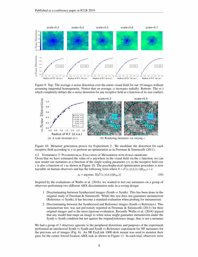
6.3 MetamerModel Comparison

The following table summarizes the main similarities and differences across all current models:

Model FS (2011) CNN-Synthesis (2018) SideEye (2017) NF (Ours)Feed-Forward - - X X

Input Noise Noise Image ImageMulti-Resolution X X - -Texture Statistics Steerable Pyramid VGG19 conv-11,21,31,41,51 Steerable Pyramid VGG19 relu41

Style Transfer Portilla & Simoncelli Gatys et al. Rosenholtz et al. Huang & BelongieFoveated Pooling X X (Implicit via FCN) X

Decoder (trained on) - - metamers/mongrels imagesMoveable Fovea X X X X

Use of Noise Initialization Initialization - PerturbationNon-Deterministic X X - X

Direct Computable Inverse - - (Implicit via FCN) XRendering Time hours minutes miliseconds seconds

Image type scenes scenes/texture scenes scenesCritical Scaling (vs Synth) 0.46 ∼ {0.39/0.41} Not Required 0.5

Critical Scaling (vs Reference) Not Available ∼ {0.2/0.35} Not Required 0.24Experimental design ABX Oddball - ABX

Reference Image in Exp. Metamer Original - Compressed via DecoderNumber of Images tested 4 400 - 10

Trials per observers ∼ 1000 ∼ 1000 - ∼ 3000

Table 1: Metamer Model comparison

Freeman & SimoncelliOriginal NeuroFoveaReference

Figure 15: Algorithmic (top) and visual (bottom) comparisons between our metamers and a samplefrom Freeman & Simoncelli (2011) for a scaling factor of 0.3. Each model has it’s own limitations:The FS model can not directly compute an inverse of the encoded representation to generate a metamer,requiring an iterative gradient descent procedure. Our NF model is limited by the capacity of theencoder-decoder architecture as it does not achieve lossless compression (perfect reconstruction).

1We remove central regions with an area smaller than 100 pixels, and group them into the fovea

16


Encoded Space

Perceptual Space

Image Space

Encoded Space

Perceptual Space

Image Space

Sample Metamer A Sample Metamer B Perceptual Space

The distance in green between a V1 metamer and the content image is the same as the two V2

metamers, potentially explaining how they are perceptually indistinguishable to each other at different

scaling factors given the type of ABX task.

A

B

Figure 16: Decomposition and overview of the metamer generation process in the Image space, theEncoded space and the Perceptual space. The original image patch is coded in blue, the V1 metamersare coded in purple, and the V2 metamers are coded in pink. Dark brown represents the initial whitenoise that is later stylized via AdaIN through S(◦). Note that these two points are far away to eachother in image space, but quite closeby in perceptual space as they are also ‘metameric’ to each other.They are not placed on the actual encoded manifold since these points are not in the near vicinity ofeither C nor S(N), as they have no scene-like structure. The interpolation for maximal distortion isdone along the line between C and S(N), these are the points in blue and red in the encoded spacewhich represent the extremes of α = 0.0 and α = 1.0 respectively.

6.4 Interpretability of V1 and V2 Metamers

In Figure 16, we illustrate the metamer generation process for two sample metamers, given differentnoise perturbations. Here, we decompose Figure 4 into two separate ones for each metamer giveneach noise perturbation, and provide an additional visualization of the projection of the metamers inperceptual space, gaining theoretical insight on how and why metamerism arises for the synth-vs-synthcondition in V2, and the synth-vs-reference condition in V1 as we demonstrated experimentally.

6.5 Pilot Experiments

Pro

port

ion C

orr

ect

1.0

0.9

0.8

0.7

0.6

0.5

0.4

List of Pilot Observers'LR' 'SO' 'DS' 'JZ' 'OD' 'SW'


Freeman & Simoncelli ABX task

Figure 17: Pilot Data on FS metamers.

In a preliminary psychophysical study, we ran anexperiment with a collection of 50 images and 6 ob-servers on the FS metamers. Observers performed asingle session of 200 trials of the FS metamers wherethe scale was fixed at s = 0.5. We found the follow-ing: While we found that the synthesized imageswere metameric to each other for the scaling factor of0.5, the FS metamers were not metameric to their ref-erence high-quality images at the scale of 0.5. Only asub-group of observers: ‘LR’,‘SO’,‘DS’ scored wellabove chance in terms of discriminating the imagesin the ABX task. These results are in synch with theevalutions done by Wallis et al. (2018), which variedscale and found a critical value to be less than 0.5 andrather closer to 0.25 within the range of V1.

17


6.6 Estimation of Lapse-rate (λ) per observer

The motivation behind estimating the lapse rate is to quantify how engaged was the observer in theexperiment, as well as providing a robust estimate of the parameters in the fit of the psychometricfunctions. Not accounting for lapse rate may dramatically affect the estimation of these parametersas suggested in Wichmann & Hill (2001). In general lapse rates are computed by penalizing apsychometric function ψ(◦) that ranges between some lower bound and upper bound usually [0,1].To estimate the lapse rate λ, a new ψ′(◦) is defined to have the following form:

ψ′(◦) = b + (1−b−λ)ψ(◦) (15)

Recall that for us, our psychometric fitting function ψ(◦) = PCABX(s) is defined by Equation 11 andparametrized by both the absorbing factor β0 and the critical scaling factor s0:

PCABX(s) = Φ

(d2(s)√

(6)

)Φ

(d2(s)

2

)+Φ

(−d2(s)√

(6)

)Φ

(−d2(s)

2

)(16)

where we have:

d2(s) = β0(1−s2

o

s2 )1s>s0 (17)

To compute the new ψ′(◦), we notice first that our ψ is bounded between [0.5,1], and that the new ψ′

will be a linear combination of a correct guess for a lapse, and a correct decision for a non-lapse fromwhich we obtain:

PC(s) = λ+ (1−2λ)PCABX(s) (18)

as derived in Hénaff (2018) which includes lapse rates for an AXB task. When fitting the curvesfor each of the n = 10000 bootstrapped samples, we restricted the lapse rate to vary betweenλ = [0.00,0.06] as suggested in Wichmann & Hill (2001), and found the following lapse rates:

Observer 1: λRSZQ = 0.0248±0.0209, λS S

ZQ = 0.0430±0.0228.

Observer 2: λRSAL = 0.0008±0.0062, λS S

AL = 0.0166±0.0215.

Observer 3: λRSAG = 0.0141±0.0243, λS S

AG = 0.0218±0.0236.

We later averaged these lapse rates as there is an equal probability of each type of trial to appear(Synth vs Synth, or Reference vs Synth), and refitted each curve with the new pooled lapse rateestimates λ′. Indeed, each observer did both experiments in a roving paradigm, rather than doing oneexperiment after the other – thus we should only have one estimate for lapse rate per observer. It isworth mentioning that re-performing the fits with separate lapse rates did not significantly affect theestimates of critical scaling values, as one might argue that higher lapse rates will significantly movethe critical scaling factor estimates. This is not the case as the absorbing factor β does not place anupper bound for the psychometric function at 1.

Our critical estimates of lapse rates were: λZQ = 0.0339, λAL = 0.0087, λAG = 0.0179, as shown inFigure 12.

The estimates (critical scale (s0), absorbing factor (β0) and lapse rate (λ0)) shown for the pooledobserver were obtained by averaging the estimates over the 3 observers.

18


6.7 Robustness of estimation of γ function

In this subsection we show how the perceptual optimization pipeline is robust to a selection of IQAmetrics such as MS-SSIM (multi-scale SSIM 2) from Wang et al. (2003) and IW-SSIM (informationcontent weighted SSIM) from Wang & Li (2011).

There are 3 key observations that stem from these additional results:

1. The sigmoidal natural of the γ function is found again and is also scale independent, showingthe broad applicability of our perceptual optimization scheme and how it is extendable toother IQA metrics that satisfy SSIM-like properties (upper bounded, symmetric and uniquemaximum).

2. The tuning curves of MS-SSIM and IW-SSIM look almost identical, given that IW-SSIM isnot more than a weighted version of MS-SSIM where the weighting function is the mutualinformation between the encoded representations of the reference and distortion imageacross multiple resolutions. Differences are stronger in IW-SSIM when the region overwhich it is evaluated is quite large (i.e. an entire image), however given that our poolingregions are quite small in size, the IW-SSIM score asymptotes to the MS-SSIM score. Inaddition both scores converge to very similar values given that we are averaging these scoresover the images and over all the pooling regions that lie within the same eccentricity ring.We found that ∼ 90% of the maximum α’s had the same values given the 20 point samplinggrid that we use in our optimization. Perhaps a different selection of IW hyperparameters(we used the default set), finer sampling schemes for the optimal value search, as well asaveraging over more images, may produce visible differences between both metrics.

3. The sigmoidal slope is smaller for both IW-SSIM and MS-SSIM vs SSIM, which yields moreconservative distortions (as α is smaller for each receptive field). This implies that the modelcan still create metamers at the estimated found scaling factors of 0.21 and 0.50, howeverthey may have different critical scaling factors for the reference vs synth experiment, and forthe synth vs synth experiment. Future work should focus on psychophysically finding thesecritical scaling factors, and if they still are within the range of rate of growth of receptivefield sizes of V1 and V2.

1.0

0.8

0.6

0.4

0.2

0.0

Radius of R.F. (d.v.a.)0.0 0.5 1.0 1.5 2.0 2.5 3.0

Radius of R.F. (d.v.a.)0.0 0.5 1.0 1.5 2.0 2.5 3.0

Radius of R.F. (d.v.a.)0.0 0.5 1.0 1.5 2.0 2.5 3.0


d=0.697


d=0.703


d=1.281

Figure 18: A collection of scale invariant γ(◦)’s across multiple IQA metrics for the perceptualoptimization scheme of Experiment 1. In this figure we superimpose all maximal α-noise distortionsfor each scale, and find a function that fits all the points showing that γ is indepedent of scale.

2scale in the context of SSIM is referred to resolution (as in scales of a laplacian pyramid), and is not to beconfused with the scaling factor s of our experiments which encode the rate of groth of the receptive fields.

19



1.0

0.8

0.6

0.4

0.2

0.0

Radius of R.F. (d.v.a.)0.0 0.5 1.0 1.5 2.0 2.5 3.0

Radius of R.F. (d.v.a.)0.0 0.5 1.0 1.5 2.0 2.5 3.0

Radius of R.F. (d.v.a.)0.0 0.5 1.0 1.5 2.0 2.5 3.0

Radius of R.F. (d.v.a.)0.0 0.5 1.0 1.5 2.0 2.5 3.0

Radius of R.F. (d.v.a.)0.0 0.5 1.0 1.5 2.0 2.5 3.0

1.0

0.8

0.6

0.4

0.2

0.0

d=1.240 d=1.196 d=1.363 d=1.311 d=1.355

(a) Perceptual Optimization with SSIM.


1.0

0.8

0.6

0.4

0.2

0.0

Radius of R.F. (d.v.a.)0.0 0.5 1.0 1.5 2.0 2.5 3.0

Radius of R.F. (d.v.a.)0.0 0.5 1.0 1.5 2.0 2.5 3.0

Radius of R.F. (d.v.a.)0.0 0.5 1.0 1.5 2.0 2.5 3.0

Radius of R.F. (d.v.a.)0.0 0.5 1.0 1.5 2.0 2.5 3.0

Radius of R.F. (d.v.a.)0.0 0.5 1.0 1.5 2.0 2.5 3.0

1.0

0.8

0.6

0.4

0.2

0.0

d=0.621 d=0.649 d=0.749 d=0.757 d=0.736

(b) Perceptual Optimization with MS-SSIM.


1.0

0.8

0.6

0.4

0.2

0.0

Radius of R.F. (d.v.a.)0.0 0.5 1.0 1.5 2.0 2.5 3.0

Radius of R.F. (d.v.a.)0.0 0.5 1.0 1.5 2.0 2.5 3.0

Radius of R.F. (d.v.a.)0.0 0.5 1.0 1.5 2.0 2.5 3.0

Radius of R.F. (d.v.a.)0.0 0.5 1.0 1.5 2.0 2.5 3.0

Radius of R.F. (d.v.a.)0.0 0.5 1.0 1.5 2.0 2.5 3.0

1.0

0.8

0.6

0.4

0.2

0.0

d=0.614 d=0.640 d=0.733 d=0.758 d=0.733

(c) Perceptual Optimization with IW-SSIM.

Figure 19: Top: The maximum α-noise distortion computed per pooling region, and collapsed overall images for each IQA metric. Bottom: When averaging across all the pooling regions for eachretinal eccentricity, we find that the γ function is invariant to scale as in our original experiment –suggesting that our perceptual optimization scheme is flexible across IQA metrics.

20



0

200

400

600

800

1000

Num

ber

of

Perm

ute

d S

am

ple

s

Difference Distribution0.25-0.15 -0.05 0.05 0.15










0

200

400

600

800

1000

Num

ber

of

Perm

ute

d S

am

ple

s






0

200

400

600

800

1000

Num

ber

of

Perm

ute

d S

am

ple

s

Figure 20: A permutation test was ran and determined that each γ function is also scale independentunder the 99% confidence interval (CI), as we increased the CI to account for false discovery rates(FDR). Indeed, when we perform the permutation tests and use a 95% confidence interval (shown inthe figure with the vertical lines in cyan), all curves except for MS-SSIM and IW-SSIM only for thescaling factor of 0.3 show a significant difference p ∼ 0.02 (non FDR-corrected), potentially due tosmall receptive field sizes, which bias the estimates. All other differences in the d parameter of thesigmoid function, with respect to the average fitted sigmoid, are statistically insignificant.

21

Towards Metamerism via Foveated S Transfer

Documents