Towards a Spectral Theory for Simplicial Complexes by John Steenbergen Department of Mathematics Duke University Date: Approved: Sayan Mukherjee, Supervisor John Harer Mauro Maggioni Ezra Miller Dissertation submitted in partial fulfillment of the requirements for the degree of Doctor of Philosophy in the Department of Mathematics in the Graduate School of Duke University 2013

Welcome message from author
This document is posted to help you gain knowledge. Please leave a comment to let me know what you think about it! Share it to your friends and learn new things together.
Transcript

Towards a Spectral Theory for Simplicial
Complexes
by
John Steenbergen
Department of MathematicsDuke University
Date:Approved:
Sayan Mukherjee, Supervisor
John Harer
Mauro Maggioni
Ezra Miller
Dissertation submitted in partial fulfillment of the requirements for the degree ofDoctor of Philosophy in the Department of Mathematics
in the Graduate School of Duke University2013
Abstract
Towards a Spectral Theory for Simplicial Complexes
by
John Steenbergen
Department of MathematicsDuke University
Date:Approved:
Sayan Mukherjee, Supervisor
John Harer
Mauro Maggioni
Ezra Miller
An abstract of a dissertation submitted in partial fulfillment of the requirements forthe degree of Doctor of Philosophy in the Department of Mathematics
in the Graduate School of Duke University2013

Copyright c© 2013 by John SteenbergenAll rights reserved except the rights granted by the
Creative Commons Attribution-Noncommercial Licence
Abstract
In this dissertation we study combinatorial Hodge Laplacians on simplicial com-
plexes using tools generalized from spectral graph theory. Specifically, we consider
generalizations of graph Cheeger numbers and graph random walks. The results in
this dissertation can be thought of as the beginnings of a new spectral theory for
simplicial complexes and a new theory of high-dimensional expansion.
We first consider new high-dimensional isoperimetric constants. A new Cheeger-
type inequality is proved, under certain conditions, between an isoperimetric constant
and the smallest eigenvalue of the Laplacian in codimension 0. The proof is similar
to the proof of the Cheeger inequality for graphs. Furthermore, a negative result is
proved, using the new Cheeger-type inequality and special examples, showing that
certain Cheeger-type inequalities cannot hold in codimension 1.
Second, we consider new random walks with killing on the set of oriented sim-
plexes of a certain dimension. We show that there is a systematic way of relating
these walks to combinatorial Laplacians such that a certain notion of mixing time
is bounded by a spectral gap and such that distributions that are stationary in a
certain sense relate to the harmonics of the Laplacian. In addition, we consider the
possibility of using these new random walks for semi-supervised learning. An algo-
rithm is devised which generalizes a classic label-propagation algorithm on graphs to
simplicial complexes. This new algorithm applies to a new semi-supervised learning
problem, one in which the underlying structure to be learned is flow-like.
iv

This dissertation is dedicated to my parents, who always supported my education.
v

Contents
Abstract iv
List of Figures viii
Acknowledgements x
1 Introduction 1
2 History 4
2.1 Cheeger Numbers . . . . . . . . . . . . . . . . . . . . . . . . . . . . . 4
2.2 Random Walks . . . . . . . . . . . . . . . . . . . . . . . . . . . . . . 6
3 Isoperimetric Methods in the Spectral Theory of Simplicial Com-plexes 9
3.1 Introduction . . . . . . . . . . . . . . . . . . . . . . . . . . . . . . . . 9
3.1.1 Background . . . . . . . . . . . . . . . . . . . . . . . . . . . . 9
3.1.2 Main Results . . . . . . . . . . . . . . . . . . . . . . . . . . . 10
3.1.3 Related Work . . . . . . . . . . . . . . . . . . . . . . . . . . . 11
3.2 Main Results . . . . . . . . . . . . . . . . . . . . . . . . . . . . . . . 12
3.2.1 Simplicial Complexes . . . . . . . . . . . . . . . . . . . . . . . 12
3.2.2 Chain and Cochain Complexes . . . . . . . . . . . . . . . . . . 13
3.2.3 Laplacians and Eigenvalues . . . . . . . . . . . . . . . . . . . 15
3.2.4 Cheeger Numbers . . . . . . . . . . . . . . . . . . . . . . . . . 16
3.2.5 Additional Notation and Preliminary Results . . . . . . . . . . 17
3.2.6 Main Results . . . . . . . . . . . . . . . . . . . . . . . . . . . 21
vi
3.3 Relation to Graphs . . . . . . . . . . . . . . . . . . . . . . . . . . . . 34
3.4 Discussion and Open Problems . . . . . . . . . . . . . . . . . . . . . 36
4 Stochastic Methods in the Spectral Theory of Simplicial Complexes 40
4.1 Introduction . . . . . . . . . . . . . . . . . . . . . . . . . . . . . . . . 40
4.1.1 Background . . . . . . . . . . . . . . . . . . . . . . . . . . . . 40
4.1.2 Motivation . . . . . . . . . . . . . . . . . . . . . . . . . . . . . 42
4.1.3 Summary of Results . . . . . . . . . . . . . . . . . . . . . . . 43
4.1.4 Related Work . . . . . . . . . . . . . . . . . . . . . . . . . . . 44
4.2 Definitions . . . . . . . . . . . . . . . . . . . . . . . . . . . . . . . . . 45
4.2.1 Simplicial Complexes . . . . . . . . . . . . . . . . . . . . . . . 45
4.2.2 Chain and Cochain Complexes . . . . . . . . . . . . . . . . . . 47
4.2.3 The Laplacian . . . . . . . . . . . . . . . . . . . . . . . . . . . 48
4.3 Random walks and the k-Laplacian . . . . . . . . . . . . . . . . . . . 52
4.4 Random walks with Neumann boundary conditions . . . . . . . . . . 61
4.5 Other Random Walks . . . . . . . . . . . . . . . . . . . . . . . . . . . 64
4.6 Examples of random walks . . . . . . . . . . . . . . . . . . . . . . . . 68
4.6.1 Triangle complexes . . . . . . . . . . . . . . . . . . . . . . . . 68
4.6.2 Label propagation on edges . . . . . . . . . . . . . . . . . . . 71
4.6.3 Experiments . . . . . . . . . . . . . . . . . . . . . . . . . . . . 78
4.7 Discussion . . . . . . . . . . . . . . . . . . . . . . . . . . . . . . . . . 80
Bibliography 83
Biography 86
vii

List of Figures
3.1 An example of ∂(R) and δ(R). . . . . . . . . . . . . . . . . . . . . . . 14
3.2 An example of ∂(Z2) and δ(Z2). . . . . . . . . . . . . . . . . . . . . . 14
3.3 The fundamental polygon of RP 2. . . . . . . . . . . . . . . . . . . . . 23
3.4 The family of graphs Gk. . . . . . . . . . . . . . . . . . . . . . . . . . 23
3.5 The simplicial 2-complex Y . . . . . . . . . . . . . . . . . . . . . . . . 24
3.6 The chain φ ∈ C2(Z2) that minimizes h2. The chain assigns a 1 to allcolored triangles and 0 to all else. . . . . . . . . . . . . . . . . . . . . 24
3.7 The eigenvector f ∈ C2(R) of λ2. The function f assigns values near1 for the central triangles and values near 0 to all other triangles. . . 25
3.8 Making Dirichlet boundary conditions explicit. . . . . . . . . . . . . . 26
3.9 The first four iterations X1, X2, X3, X4 of Xk in dimension 2. The2-simplexes have been shaded according to their depth. . . . . . . . . 29
3.10 The first three iterations Y1, Y2, Y3 of Yk in dimension 2. The 2-simplexes have been shaded according to their depth. . . . . . . . . . 33
3.11 The fundamental polygon of RP 2, a triangulation, and the dual graphof the triangulation. . . . . . . . . . . . . . . . . . . . . . . . . . . . . 37
4.1 Making the Dirichlet boundary condition explicit, and translating intoa graph. . . . . . . . . . . . . . . . . . . . . . . . . . . . . . . . . . . 70
4.2 A 2-complex with a labelled edge. . . . . . . . . . . . . . . . . . . . . 79
4.3 Label propagation with L = Lup1 . . . . . . . . . . . . . . . . . . . . . 79
4.4 Label propagation with L = Ldown1 . . . . . . . . . . . . . . . . . . . . 80
4.5 Label propagation with L = L1. . . . . . . . . . . . . . . . . . . . . . 80
viii

4.6 A 2-complex with two different labels on four edges. . . . . . . . . . . 81
4.7 Label propagation with L = L1. . . . . . . . . . . . . . . . . . . . . . 81
ix

Acknowledgements
I’d first like to acknowledge my parents, who always supported my education, and
my high school math tutor Shail Ganith, under whom I learned much more than I
should have. I’d also like to thank my wife, without whom I would not be where I am
today, my Uncle Tuck and Aunt Tish, for advice and support, and my two children
Julia and Charles, for comedic relief.
In addition, I’d like to acknowledge Yuan Yao, Yuriy Mileyko, Prakash Balachan-
dran, Mikhail Belkin, Anna Gundert, Matt Kahle, Kevin McGoff, Afonso Bandeira,
Amit Singer, Dominic Dotterrer, Anil Hirani, William Allard, John Harer, Mauro
Maggioni, and Ezra Miller for discussions and insight. I’m pleased to to acknowledge
support from Duke University, including a Duke Endowment Fellowship, and from
grant NSF CCF-1209155.
x

1
Introduction
This dissertation is concerned with the spectral theory of combinatorial Hodge Lapla-
cians on simplicial complexes. Simplicial complexes are discrete, combinatorial ob-
jects that have long been used to approximate manifolds and study their topology.
The Hodge Laplacians of a smooth manifold, defined using the de Rham complex,
are discretely approximated by the combinatorial Laplacians on simplcial complexes.
Thus, combinatorial Laplacians lie in the realm of discrete and computational geom-
etry.
In addition, combinatorial Laplacians generalize to higher order the more basic
notion of the Laplacian of a graph. Historically, the graph Laplacian has been well-
studied and well-applied to modern problems. In 1992, Fan Chung published a book
called Spectral Graph Theory that promised, rather poetically, to tell “an intertwined
tale of eigenvalues and their use in unlocking a thousand secrets about graphs,” and
to show “ how, through eigenvalues, theory and applications in communications and
computer science come together in symbiotic harmony.” Indeed, the book lived up to
these promises and, more than twenty years later, research in theoretical and applied
spectral graph theory is as active as ever.
1
Compared to the graph Laplacian, combinatorial Laplacians are ill-understood
and infrequently applied. The long-running success of spectral graph theory suggests
that this need not be the case. It seems reasonable to hope that, just as the graph
Laplacian generalizes to higher orders, perhaps spectral graph theory generalizes to
higher orders as well. This simple idea has recently gained traction in the literature,
and it forms the basis of this dissertation.
The primary difficulty in generalized graph theory to simplicial complexes is the
importance of orientation in higher dimensions. When working with graphs the
main objects are the vertices, and there is no meaningful notion of orientation for
vertices. We meaningfully can ask whether two vertices are connected by an edge, but
not whether those two vertices are similarly or dissimilarly oriented. However, the
geometry of a simplicial complex is only revealed when considering the different ways
of orienting edges, triangles, tetrahedrons, etc., and determining how all the different
oriented objects relate to each other. Since there are always two orientations of an
edge, triangle, etc., it is unsurprising that there are certain “dualities” embedded
in the geometry of simplicial complexes. For instance, in general the combinatorial
Laplacian decomposes into two complementary “halves”, the exception being the
graph Laplacian (or 0-order Laplacian) and the highest-order Laplacian (or m-order
Laplacian for a simplicial complex of dimension m). Therefore, it is possible that
when generalizing spectral graph theory to higher dimensions, only one “half” of the
spectral theory of combinatorial Laplacians will be revealed. Much of the work in
this dissertation is spent overcoming precisely this kind of one-sided generalization
to give a more comprehensive picture of the spectral theory of simplicial complexes.
The dualities that appear in higher dimensions on simplicial complexes are most
intuitively understood by considering the analogous case of continuous manifolds.
For manifolds with boundary, Hodge theory breaks down and the Laplacian must be
restricted to a subspace of forms in order for its kernel to reflect the cohomology of the
2
space. According to the famous Lefschetz duality theorem, there are two different
subspaces to choose from: the subspace of Neumann forms and the subspace of
Dirichlet forms. As their name implies, Neumann forms satisfy a sort of “Neumann”
boundary condition while Dirichlet forms satisfy a “Dirichlet” boundary condition. If
the Laplacian is restricted to Neumann forms, the resulting kernel is then isomorphic
to absolute cohomology, and if it is restricted to Dirichlet forms, the resulting kernel
is isomorphic to relative cohomology (i.e., cohomology relative to the boundary of
the manifold). Spectral graph theory, in its most straightforward formulation, has
always been intuitively identified with Neumann geometry. In this way, attempts to
generalize spectral graph theory to higher dimensions have initially resulted in an
exclusively Neumann perspective on the geometry of simplicial complexes. Perhaps
the single biggest theoretical contribution this dissertation makes to the literature is
it provides the missing Dirichlet perspective on the geometry of simplicial complexes.
3

2
History
In this section, we provide some historical context for the research presented in
Chapters 3 and 4. We do not yet delve into the most directly relevant literature;
that will be referred to as needed in Chapters 3 and 4.
2.1 Cheeger Numbers
Cheeger numbers were first defined on manifolds by Jeff Cheeger (after whom Cheeger
numbers are named) in Cheeger (1970). Originally, only one Cheeger number was
defined for manifolds, with its definition independent on whether the manifold had a
boundary. Further work by Buser in ? showed that in fact two separate definitions
can be made, each independent of whether the manifold has a boundary. These are
as follows:
Definition 1. Let M be a d-dimensional Riemannian manifold, with or without
boundary. Set
hN := inf∅(S(M
A(∂S \ ∂M)
min{Vol(S),Vol(M \ S)}and hD := inf
∅(S⊆M
A(∂S)
Vol(S)
4

where the infimums are taken over all d-dimensional submanifolds S, A() denotes (d−
1)-dimensional area, Vol() denotes d-dimensional volume, and A(∂S \ ∂M) denotes
the area of the part of the boundary of S that doesn’t overlap with the boundary of
M .
This is not the only way of defining Cheeger numbers. If one wants the infimums
to be attained, for instance, one can replace submanifolds in the definition with
Z2-valued currents (as studied in geometric measure theory).
What Cheeger and Buser proved is that
λ∗ ≥1
4h2∗
for ∗ = N,D where λN is the second smallest eigenvalue of the Laplace-Beltrami
operator restricted to functions satisfying Neumann boundary conditions and λD is
the smallest eigenvalue of the Laplace-Beltrami operator restricted to functions sat-
isfying Dirichlet boundary conditions. This inequality is called Cheeger’s inequality.
Note that M is disconnected if and only if hN = λN = 0, and similarly hD = λD = 0
if and only if some connected component M1 of M has no boundary and is orientable.
Starting with Cheeger’s original paper, researchers have wondered if there is
some higher-order analogue of Cheeger’s inequality, that is, an inequality relating the
spectral gap of a higher-order Hodge Laplacian to a Cheeger number. The underlying
challenge here is that in general the spectral gaps of higher-order Hodge Laplacians
can vary independently of each other (see Guerini and Savo (2003)). Thus, Cheeger
number as originally defined can only reasonably relate to one spectral gap at a time.
If a Cheeger inequality is to be found for higher-order Laplacians, it stands to reason
that new higher-dimensional Cheeger numbers need to be defined.
5
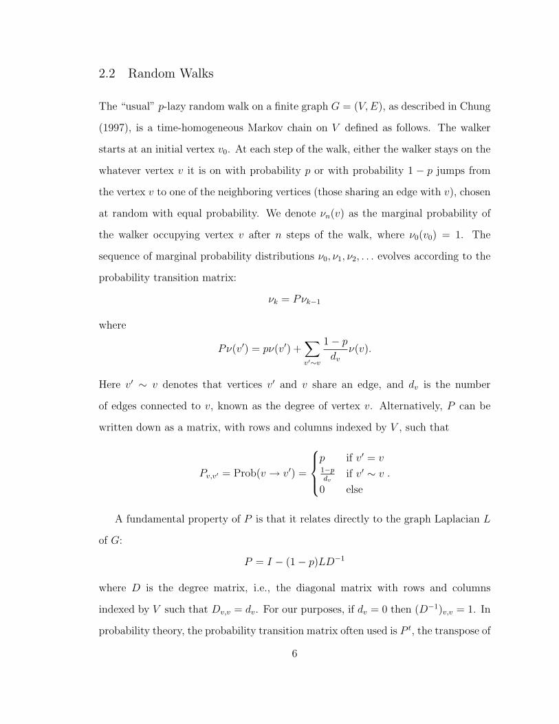
2.2 Random Walks
The “usual” p-lazy random walk on a finite graph G = (V,E), as described in Chung
(1997), is a time-homogeneous Markov chain on V defined as follows. The walker
starts at an initial vertex v0. At each step of the walk, either the walker stays on the
whatever vertex v it is on with probability p or with probability 1 − p jumps from
the vertex v to one of the neighboring vertices (those sharing an edge with v), chosen
at random with equal probability. We denote νn(v) as the marginal probability of
the walker occupying vertex v after n steps of the walk, where ν0(v0) = 1. The
sequence of marginal probability distributions ν0, ν1, ν2, . . . evolves according to the
probability transition matrix:
νk = Pνk−1
where
Pν(v′) = pν(v′) +∑v′∼v
1− pdv
ν(v).
Here v′ ∼ v denotes that vertices v′ and v share an edge, and dv is the number
of edges connected to v, known as the degree of vertex v. Alternatively, P can be
written down as a matrix, with rows and columns indexed by V , such that
Pv,v′ = Prob(v → v′) =
p if v′ = v1−pdv
if v′ ∼ v
0 else
.
A fundamental property of P is that it relates directly to the graph Laplacian L
of G:
P = I − (1− p)LD−1
where D is the degree matrix, i.e., the diagonal matrix with rows and columns
indexed by V such that Dv,v = dv. For our purposes, if dv = 0 then (D−1)v,v = 1. In
probability theory, the probability transition matrix often used is P t, the transpose of
6

P , such that νk = νk−1P . However, when relating probability transition matrices to
Laplacians it is more convenient to use so-called left stochastic matrices as opposed
to right stochastic matrices.
As a result of the above equation, P (and, hence, the random walk described
above) can be studied purely in terms of properties of the graph Laplacian L. For
instance, it is a basic fact that the spectrum of LD−1 is contained in the interval [0, 2].
The lower bound of 0 is always contained in the spectrum and 2 is an eigenvalue if and
only if the graph is bipartite. Thus, the spectrum of P is contained in [1−2(1−p), 1],
1 is always an eigenvalue of P , and −1 is an eigenvalue if and only if p = 0 and the
graph contains a bipartite connected component. This implies the existence of a
stationary distribution of the random walk, and implies that νn = P nν0 converges
to a stationary distribution for any initial distribution ν0 if and only if p > 0 or
p = 0 and the graph does not contain any bipartite connected component. If p = 0
and the graph contains a bipartite connected component, then all of the vertices
in the bipartite connected component are 2-periodic states for the Markov chain.
Furthermore, if the random walk starts at an initial vertex v0 (so ν0(v0) = 1) and νn
converges, then G is connected (and the Markov chain is irreducible) if and only if
limn→∞ νn(v) > 0 for all v ∈ V . Finally, it can be proved that if p ≥ 12, then
‖νk − limn→∞
νn‖2 = O([1− (1− p)λ]k)
where ‖·‖2 is the Euclidean norm and λ is the smallest nonzero eigenvalue of LD−1.
These results, and other like them, have had many applications in theoretical and
applied mathematics. As a result, it has long been an open question whether higher-
dimensional random walks can be defined on simplicial complexes which have a sim-
ilar relationship with the spectral theory of higher-order Laplacians. The difficulty,
historically, has not been simply in defining random walks on higher-dimensional
simplexes (edges, triangle, etc.), but in drawing any connection with higher-order
7

Laplacians. Unlike the graph Laplacian, when higher-order Laplacians are written
down as matrices (in the “usual” way), they contain both positive and negative
off-diagonal entries. This means that for any probability transition matrix P , an
equation like P = I − (1 − p)LD−1 can never hold, since P by definition has only
positive entries. Thus, new methods are needed to bridge the gap between the
stochastic and spectral theories of simplicial complexes.
8

3
Isoperimetric Methods in the Spectral Theory ofSimplicial Complexes
3.1 Introduction
3.1.1 Background
The Cheeger inequality (see Cheeger (1970); Buser (1980)) is a classic result that
relates the isoperimetric constant of a manifold (with or without boundary) to the
spectral gap of the Laplace-Beltrami operator. An analog of the manifold result
was also found to hold on graphs (see Alon and Milman (1985); Alon (1986); Mohar
(1989)) and is a prominent result in spectral graph theory. Given a graph G with
vertex set V , the Cheeger number is the following isoperimetric constant
h := min∅(S(V
|δS|min{|S|, |S|}
where δS is the set of edges connecting a vertex in S with a vertex in S = V \ S.
The Cheeger inequality on the graph relates the Cheeger number h to the algebraic
connectivity λ (see Fiedler (1973)) which is the the second eigenvalue of the graph
9

Laplacian. It states that
2h ≥ λ ≥ h2
2 maxv∈V dv
where dv is the number of edges connected to vertex v (also called the degree of the
vertex). For more background on the Cheeger inequality see Chung (1997).
A key motivation for studying the Cheeger inequality has been understanding
graph expansion in the sense of Hoory et al. (2006). A family of regular graphs of
increasing size is said to be expanding if the algebraic connectivity λ of the graphs
stay bounded away from 0, which, by way of the Cheeger inequality, is equivalent
to saying that the Cheeger numbers h of the graphs stay bounded away from 0.
Thus, h is used to study the expansion properties of graphs. A generalization of
the Cheeger number to higher dimensions on simplicial complexes, based on ideas
in Linial and Meshulam (2006); Meshulam and Wallach (2009), was defined and
expansion properties studied in Dotterrer and Kahle (2012) via cochain complexes.
In addition, it has been known since Eckmann (see Eckmann (1945)) that the graph
Laplacian generalizes to higher dimensions on simplicial complexes. In particular
one can generalize the notion of algebraic connectivity to higher dimensions using
the cochain complex and relate an eigenvalue of the k-dimensional Laplacian to the
k-dimensional Cheeger number. This raises the question of whether the Cheeger
inequality has a higher-dimensional analog.
3.1.2 Main Results
In this chapter we examine the combinatorial Laplacian which is derived from a
chain complex and a cochain complex. Precise definitions of the object studied and
the results are given in section 2. We first state our negative result: for the cochain
complex a natural Cheeger inequality does not hold. For an m-dimensional simplicial
complex we denote λm−1 as the analog of the spectral gap for dimension m − 1 on
10
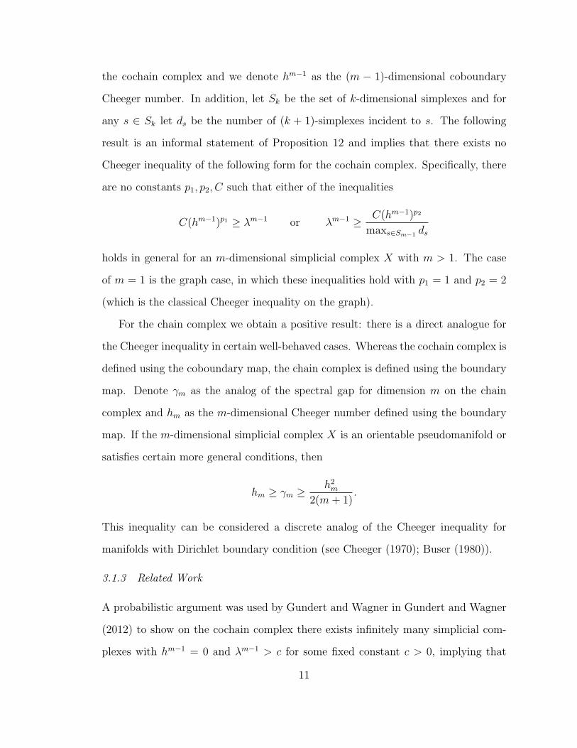
the cochain complex and we denote hm−1 as the (m − 1)-dimensional coboundary
Cheeger number. In addition, let Sk be the set of k-dimensional simplexes and for
any s ∈ Sk let ds be the number of (k + 1)-simplexes incident to s. The following
result is an informal statement of Proposition 12 and implies that there exists no
Cheeger inequality of the following form for the cochain complex. Specifically, there
are no constants p1, p2, C such that either of the inequalities
C(hm−1)p1 ≥ λm−1 or λm−1 ≥ C(hm−1)p2
maxs∈Sm−1 ds
holds in general for an m-dimensional simplicial complex X with m > 1. The case
of m = 1 is the graph case, in which these inequalities hold with p1 = 1 and p2 = 2
(which is the classical Cheeger inequality on the graph).
For the chain complex we obtain a positive result: there is a direct analogue for
the Cheeger inequality in certain well-behaved cases. Whereas the cochain complex is
defined using the coboundary map, the chain complex is defined using the boundary
map. Denote γm as the analog of the spectral gap for dimension m on the chain
complex and hm as the m-dimensional Cheeger number defined using the boundary
map. If the m-dimensional simplicial complex X is an orientable pseudomanifold or
satisfies certain more general conditions, then
hm ≥ γm ≥h2m
2(m+ 1).
This inequality can be considered a discrete analog of the Cheeger inequality for
manifolds with Dirichlet boundary condition (see Cheeger (1970); Buser (1980)).
3.1.3 Related Work
A probabilistic argument was used by Gundert and Wagner in Gundert and Wagner
(2012) to show on the cochain complex there exists infinitely many simplicial com-
plexes with hm−1 = 0 and λm−1 > c for some fixed constant c > 0, implying that
11

one side of the Cheeger inequality cannot hold in general. However, this construc-
tion requires the complexes to have torsion in their integral homology groups due
to the way hm−1 and λm−1 relate to cohomology. In this chapter we show that even
for torsion-free simplicial complexes there exist counterexamples that rule out both
sides of a Cheeger inequality.
The analysis of the chain complex in this chapter is related to a paper by Fan
Chung, Chung (2007), which introduces a notion of a Cheeger number on graphs with
the analog of a Dirichlet boundary condition. We provide a detailed comparison in
section 3.3.
Finally, it should be mentioned that the authors in Parzanchevski et al. (2012)
prove a one-sided Cheeger-type inequality for λm−1 using a modified higher-dimensional
Cheeger number. The modified Cheeger number used is nonzero, and the inequality
fails, unless the simplicial complex has complete skeleton.
3.2 Main Results
3.2.1 Simplicial Complexes
Since the concept of a Cheeger inequality is strongly associated to manifolds we focus
in this chapter on abstract simplicial complexes that are analogous to well-behaved
manifolds. In particular, we will focus on simplicial complexes that have geometric
realizations homeomorphic to a Euclidean ball Bm := {x ∈ Rm : ‖x‖2 ≤ 1}. We will
call such complexes simplicial m-balls
By a simplicial complex we mean an abstract finite simplicial complex. Simplicial
complexes generalize the notion of a graph to higher dimensions. Given a set of
vertices V , any nonempty subset σ ⊆ V of the form σ = {v0, v1, . . . , vk} is called a
k-dimensional simplex, or k-simplex. A simplicial complex X is a finite collection of
simplexes of various dimensions such that X is closed under inclusion, i.e., τ ⊆ σ
and σ ∈ X implies τ ∈ X.
12
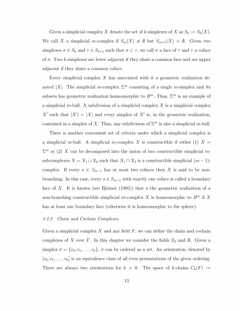
Given a simplicial complex X denote the set of k-simplexes of X as Sk := Sk(X).
We call X a simplicial m-complex if Sm(X) 6= ∅ but Sm+1(X) = ∅. Given two
simplexes σ ∈ Sk and τ ∈ Sk+1 such that σ ⊂ τ , we call σ a face of τ and τ a coface
of σ. Two k-simplexes are lower adjacent if they share a common face and are upper
adjacent if they share a common coface.
Every simplicial complex X has associated with it a geometric realization de-
noted |X|. The simplicial m-complex Σm consisting of a single m-simplex and its
subsets has geometric realization homeomorphic to Bm. Thus, Σm is an example of
a simplicial m-ball. A subdivision of a simplicial complex X is a simplicial complex
X ′ such that |X ′| = |X| and every simplex of X ′ is, in the geometric realization,
contained in a simplex of X. Thus, any subdivision of Σm is also a simplicial m-ball.
There is another convenient set of criteria under which a simplicial complex is
a simplicial m-ball. A simplicial m-complex X is constructible if either (1) X =
Σm or (2) X can be decomposed into the union of two constructible simplicial m-
subcomplexes X = X1 ∪X2 such that X1 ∩X2 is a constructible simplicial (m− 1)-
complex. If every s ∈ Sm−1 has at most two cofaces then X is said to be non-
branching. In this case, every s ∈ Sm−1 with exactly one coface is called a boundary
face of X. It is known (see Bjorner (1995)) that a the geometric realization of a
non-branching constructible simplicial m-complex X is homeomorphic to Bm if X
has at least one boundary face (otherwise it is homeomorphic to the sphere).
3.2.2 Chain and Cochain Complexes
Given a simplicial complex X and any field F , we can define the chain and cochain
complexes of X over F . In this chapter we consider the fields Z2 and R. Given a
simplex σ = {v0, v1, . . . , vk}, σ can be ordered as a set. An orientation, denoted by
[v0, v1, . . . , vk] is an equivalence class of all even permutations of the given ordering.
There are always two orientations for k > 0. The space of k-chains Ck(F ) :=
13

δ1(R) ∂2(R)v1
v2
v4
v3
v1
v2
v4
v3
v1
v2
v4
v3δ1(R) ∂2(R)
3[v2, v1] + 4[v3, v1] + 2[v3, v2] [v1, v3, v2] + 2[v2, v4, v3] [v1, v3] + [v2, v1] + 3[v3, v2]
+2[v2, v4] + 2[v4, v3]
4
3
2
0
0
1
1
3
2
2
1 2
Figure 3.1: An example of ∂(R) and δ(R).
v1
v2
v4
v3
v1
v2
v4
v3
v1
v2
v4
v3
δ1(Z2) ∂2(Z2)
[v1, v2, v3] + [v2, v3, v4]δ1(Z2) ∂2(Z2)
[v1, v2] + [v1, v3] + [v2, v3] [v1, v2] + [v1, v3]
+[v2, v4] + [v3, v4]
1
1 0
1
0
1
1
1 1
0
1
1
Figure 3.2: An example of ∂(Z2) and δ(Z2).
Ck(X;F ) is the vector space of linear combinations of oriented k-simplexes with
coefficients in F , with the stipulation that the two orientations of a simplex are
negatives of each other in Ck(F ). The space of k-cochains Ck(F ) := Ck(X;F ) is then
defined to be the vector space dual to Ck(F ). These spaces are isomorphic and we will
make no distinction between them. The boundary map ∂k(F ) : Ck(F )→ Ck−1(F ) is
defined on the basis elements [v0, . . . , vk] as
∂k[v0, . . . , vk] =k∑i=0
(−1)i[v0, . . . , vi−1, vi+1, . . . , vk]
The coboundary map δk−1(F ) : Ck−1(F )→ Ck(F ) is then defined to be the transpose
of the boundary map. When there is no confusion, we will denote the boundary and
coboundary maps by ∂ and δ. It is easy to see that ∂∂ = δδ = 0, so that (Ck(F ), ∂k)
and (Ck(F ), δk) form chain and cochain complexes. See Figures 3.1 and 3.2 for
examples of ∂ and δ on real and Z2 chains/cochains.
When F = Z2, positive and negative have no meaning and therefore no distinction
14
is made between different orientations. In particular, it is possible to identify Ck(Z2)
and Ck(Z2) with Sk as sets. Throughout this chapter, we will identify a k-chain/k-
cochain φ over Z2 with the subset φ ⊂ Sk of k-simplexes to which φ assigns the
coefficient 1 (as opposed to 0).
The homology and cohomology vector spaces of X over F are
Hk(F ) := Hk(X;F ) =ker ∂k
im ∂k+1
and Hk(F ) := Hk(X;F ) =ker δk
im δk−1.
It is known from the universal coefficient theorem that Hk(F ) is the vector space
dual to Hk(F ).
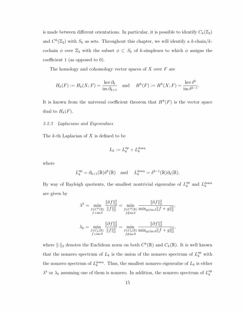
3.2.3 Laplacians and Eigenvalues
The k-th Laplacian of X is defined to be
Lk := Lupk + Ldown
k
where
Lupk = ∂k+1(R)δk(R) and Ldown
k = δk−1(R)∂k(R).
By way of Rayleigh quotients, the smallest nontrivial eigenvalue of Lupk and Ldown
k
are given by
λk = minf∈Ck(R)f⊥im δ
‖δf‖22
‖f‖22
= minf∈Ck(R)f /∈im δ
‖δf‖22
ming∈im δ‖f + g‖22
,
λk = minf∈Ck(R)f⊥im ∂
‖∂f‖22
‖f‖22
= minf∈Ck(R)f /∈im ∂
‖∂f‖22
ming∈im ∂‖f + g‖22
,
where ‖·‖2 denotes the Euclidean norm on both Ck(R) and Ck(R). It is well known
that the nonzero spectrum of Lk is the union of the nonzero spectrum of Lupk with
the nonzero spectrum of Ldownk . Thus, the smallest nonzero eigenvalue of Lk is either
λk or λk assuming one of them is nonzero. In addition, the nonzero spectrum of Lupk
15
is the same as the nonzero spectrum of Ldownk+1 . Thus, λk = λk+1 whenever λk, λk+1
are both nonzero.
The relationship between eigenvalues and homology/cohomology is as follows:
λk = 0 λk = 0m and m
Hk(R) 6= 0 Hk(R) 6= 0.
If we pass to the reduced cochain complex, λ0 becomes the algebraic connectivity
(or Fiedler number) of a graph (see Fiedler (1973)) and λ0 = 0⇔ H0(R) 6= 0.
3.2.4 Cheeger Numbers
Higher-dimensional Cheeger numbers were first stated in Dotterrer and Kahle (2012)
to capture a higher-dimensional notion of expanders. They are defined via the
coboundary map as follows:
Definition 2. Let ‖·‖ denote the Hamming norm on Ck(Z2). The k-th (coboundary)
Cheeger number of X is
hk := minφ∈Ck(Z2)φ/∈im δ
‖δφ‖minψ∈im δ‖φ+ ψ‖
.
A similar definition can be given for the boundary map.
Definition 3. Let ‖·‖ also denote the Hamming norm on Ck(Z2). The k-th boundary
Cheeger number of X is
hk := minφ∈Ck(Z2)φ/∈im ∂
‖∂φ‖minψ∈im ∂‖φ+ ψ‖
.
The relationship between Cheeger numbers and homology/cohomology is as fol-
lows:
16

hk = 0 hk = 0m and m
Hk(Z2) 6= 0 Hk(Z2) 6= 0 .
If we pass to the reduced cochain complex, h0 becomes the Cheeger number of a
graph (see Dotterrer and Kahle (2012)) and h0 = 0⇔ H0(Z2) 6= 0.
Often, we speak of a cochain that attains the minimum in the definition of the
Cheeger number (in the graph case these are Cheeger cuts). We will say that φ ∈
Ck(Z2) attains hk if hk = ‖δφ‖‖φ‖ . The same terminology will be used for hk.
3.2.5 Additional Notation and Preliminary Results
Here we collect some interesting results concerning Cheeger numbers which will be
needed later in section 3.2.6. Lemma 4 says that h1 has a very simple interpretation
in terms of the diameter of the simplicial complex. Lemma 6 says that hm−1 also has
a very simple interpretation in terms of the radius.
We define the diameter of a simplicial m-complex X as follows. Given two vertices
v1, v2 ∈ S0, we define the distance between them to be the quantity
dist(v1, v2) := min{‖φ‖ : φ ∈ C1(Z2) and ∂φ = v1 + v2}
Any chain φ attaining the minimum is called a geodesic. Note that for any geodesic
φ, h1 ≤ 2‖φ‖ . For our purposes, dist(v1, v2) = 0 if v1, v2 are not in the same connected
component. The diameter of X is then defined to be
diam(X) := maxv1,v2∈S0
dist(v1, v2).
As it turns out, h1 is strongly related to the diameter of a simplicial complex.
Lemma 4. Given a simplicial m-complex X with m ≥ 1 and satisfying H1(Z2) = 0,
h1 is attained by a geodesic and hence
h1 =2
diam(X)
17

.
Proof. Suppose that φ ∈ C1(Z2) attains h1. Clearly, ‖∂φ‖ must be even and nonzero.
What we will show is that we can assume ‖∂φ‖ = 2. Thinking of φ as a graph
(consisting of the edges in φ and their vertices), it is also clear that every connected
component φi of φ has ‖∂φi‖ even. For every pair of vertices in ∂φi, there exists
a geodesic in X with the given pair of vertices as its boundary. Thus, there exist
geodesics ψ1, . . . , ψq such that ∂ψj is a distinct pair of vertices in ∂φ for all j and
∂(ψ1 + · · ·+ ψq) = ∂φ. Since φ attains h1 and H1(Z2) = 0,
‖φ‖ = minψ∈im ∂
‖φ+ ψ‖ = min∂ψ=∂φ
‖ψ‖
In other words, φ is a 1-chain of smallest norm with boundary ∂φ. Thus, ‖ψ1 + · · ·+
ψq‖ ≥ ‖φ‖. Now,
h1 =‖∂φ‖‖φ‖
≥ ‖∂(ψ1 + · · ·+ ψq)‖‖ψ1 + · · ·+ ψq‖
≥ 2 + · · ·+ 2
‖ψ1‖+ · · ·+ ‖ψq‖
≥ min
{2
‖ψ1‖, . . . ,
2
‖ψq‖
}≥ h1
and therefore h1 = min{
2‖ψ1‖ , . . . ,
2‖ψq‖
}. Here we are using the general inequality
a1+a2+···+ak
b1+b2+···+bk≥ mini
ai
bi, valid for all a1, . . . , ak, b1, . . . , bk > 0. Hence, h1 = 2
‖ψj‖ for
some geodesic ψj. This completes the proof.
While the diameter is defined in terms of 1-chains, we define the radius in terms
of (m−1)-cochains as follows. Given a simplicial m-complex X, we define the depth
18

of an m-simplex σ to be
depth(σ) := min{‖φ‖ : φ ∈ Cm−1(Z2), δφ = σ}.
Any minimizing φ will be said to be a depth-attaining cochain for σ. Note that for
any such φ, hm−1 ≤ 1‖φ‖ . All m-simplexes have a defined depth when Hm(Z2) is
trivial. In this case, we define the radius of X to be
rad(X) := maxσ∈Sm
depth(σ).
Depth-attaining cochains have a very predictable structure for non-branching sim-
plicial complexes, a fact which we will use later in proving Proposition 12. Roughly
speaking, Lemma 5 says that if φ is depth-attaining for σ, then φ is a linear non-
intersecting sequence of (m− 1)-simplexes starting with a face of σ and ending with
a boundary face. For the statement and proof of this Lemma we define the star st(s)
of a simplex s to be the set of cofaces of s.
Lemma 5. Let X be a simplicial m-complex such that every s ∈ Sm−1 has at most
two cofaces. Suppose that σ ∈ Sm has depth d and φ is a depth-attaining cochain for
σ. Then there is a sequence s1, s2, . . . , sd of distinct (m−1)-simplexes and a sequence
σ = σ1, σ2, . . . , σd of distinct m-simplexes satisfying
1. φ =∑d
i=1 si,
2. st(si) = {σi, σi+1} for i < d,
3. st(sd) = {σd}.
Proof. Assume φ =∑d
i=1 si. Clearly, at least one of the si must have σ as a coface,
so WLOG we can assume s1 has σ = σ1 as a coface. If s1 is a boundary face, we
are done and d = 1. If not, then s1 has another coface σ2. In this case, if there are
no other si with σ2 as a coface then we arrive at the contradiction that δφ contains
19
σ2, i.e., δφ 6= σ. Thus, there is another si with σ2 as a coface, which we can assume
WLOG is s2.
We proceed by induction. Suppose that for k > 1 there is a sequence σ1, σ2, . . . , σk
of distinct m-simplexes such that δ(s1 + · · ·+sk−1) = σ+σk where st(si) = {σi, σi+1}
for all i. Then we can find another si, i > k, which we can assume WLOG is sk and
which has σk as a coface. If no such si exists then δφ 6= σ. If sk is a boundary face we
are done and d = k. If sk has σk+1 as a second coface and σk+1 = σi for some i < k
then si + . . .+ sk is a cocycle, but this means that δ(φ− si−· · ·− sk) = σ so φ is not
depth-attaining. Otherwise, σ1, σ2, . . . , σk+1 is a sequence of distinct m-simplexes
such that δ(s1 + · · · + sk) = σ + σk+1 where st(si) = {σi, σi+1} for all i. This leaves
us back where we started. By induction, we can continue this process until k = d
and sd is a boundary face.
Lemma 6. Let X be a simplicial m-complex with Hm−1(Z2) = 0 and Hm(Z2) = 0.
Then hm−1 is attained by a depth-attaining cochain and hence
hm−1 =1
rad(X).
Proof. Suppose ψ attains hm−1 and δψ is a sum of distinct m-simplexes σ1, . . . , σq
with depth-attaining cochains ψ1, . . . , ψq. Clearly ‖ψ‖ ≤ ‖ψ1‖+ · · ·+ ‖ψq‖, so
hm−1 =q
‖ψ‖
≥ 1 + · · ·+ 1
‖ψ1‖+ · · ·+ ‖ψq‖
≥ min
{1
‖ψ1‖, . . . ,
1
‖ψq‖
}≥ hm−1
and therefore hm−1 = min{
1‖ψ1‖ , . . . ,
1‖ψq‖
}. Here we are using the general inequality
20

a1+a2+···+ak
b1+b2+···+bk≥ mini
ai
bi, valid for all a1, . . . , ak, b1, . . . , bk > 0. Hence, hm−1 = 1
‖ψj‖ for
some depth-attainng cochain ψj. This completes the proof.
An interesting result which will not be used in this chapter is a Cheeger-type
inequality for the special case X = Σm.
Lemma 7. Recall Σm is the simplicial complex induced by an m-simplex. The fol-
lowing holds for all k.
1. hk(Σm−1) ≥ mk+2
2. hk(Σm−1) ≥ m
m−k .
The reason this result is Cheeger-type is because all the Laplacian eigenvalues of
all dimensions for Σm−1 are equal to m (this is easily seen from the characterization
of the Laplacian in Muhammad and Egerstedt (2006)). Part (1) of this Lemma
was proved by Meshulam and Wallach in Meshulam and Wallach (2009) (who, even
though they did not define the Cheeger number, still worked with its numerator and
denominator separately). Their proof can be easily modified to prove part (2) of the
Lemma.
3.2.6 Main Results
We now state the main results of this chapter – there exists a Cheeger-type inequality
in the top dimension for the chain complex but not for the cochain complex.
To state the results we need the following notion of orientational similarity.
Two oriented lower adjacent k-simplexes are dissimilarly oriented if they induce
the same orientation on the common face. In other words, if σ = [v0, . . . , vk] and
τ = [w0, . . . , wk] share the face {u0, . . . , uk−1}, then σ and τ are dissimilarly oriented
if ∂(R)σ and ∂(R)τ assign the same coefficient (+1 or −1) to the oriented simplex
21

[u0, . . . , uk−1]. Otherwise, they are said to be similarly oriented. If X is a simpli-
cial m-complex and all its m-simplices can be oriented similarly, then X is called
orientable.
We first state the positive result – there is a Cheeger-type inequality for the chain
complex.
Theorem 8. Let X be a simplicial m-complex, m > 0.
(1) Let φ ∈ Cm(Z2) minimize the quotient in
hm := minφ∈Cm(Z2)φ/∈im ∂
‖∂φ‖minψ∈im ∂‖φ+ ψ‖
.
If all m-simplexes in φ can be similarly oriented, then hm ≥ λm.
(2) Assume that every (m − 1)-dimensional simplex is incident to at most two
m-simplexes. Then
λm ≥h2m
2(m+ 1).
The first statement is the analog of the Buser inequality for graphs. The second
statement is an analog of the Cheeger inequality for graphs, as well as the Cheeger
inequality for a manifold with Dirichlet boundary conditions. The constraint that
every (m−1)-simplex has at most two cofaces enforces the boundary condition. The
hypotheses required for both inequalities are always satisfied by orientable pseudo-
manifolds.
The hypotheses required by the Theorem cannot be removed, as proved by the
following two examples.
Example 9 (Real Projective Plane). Given a triangulation X of RP 2 (see Figure
3.3) we know that H2(Z2) 6= 0 while H2(R) = 0, so that h2 = 0 6= λ2. This is due
22

to the nonorientability of RP 2. The chain φ ∈ C2(Z2) containing every m-simplex
has no boundary. However, the m-simplexes cannot all be similarly oriented, so that
there is no corresponding boundaryless chain in C2(R). As a result, the hypothesis
used in part (1) of the Theorem cannot in general be removed.
Figure 3.3: The fundamental polygon of RP 2.
Example 10. Let Gk be a graph with 2k vertices of degree one, half of which connect
to one end of an edge and the other half connect to the other end (see figure 3.4).
Clearly, h0(Gk) = 1k+1
while Lemma 4 implies h1 = 23. By the Buser inequality for
graphs, λ0 ≤ 2k+1
and since λ1 = λ0, this means that λ1 → 0. As a result, we conclude
that the hypothesis used in part (2) of the Theorem cannot be removed.
k vertices k verticesFigure 3.4: The family of graphs Gk.
The next example shows what it typically looks like when both inequalities hold.
23

Example 11. Let Y be the simplicial 2-complex shown in figure 3.5. Clearly, Y
satisfies the conditions for Theorem 8 to hold. It is not hard to compute in this
case the Z2 2-chain that minimizes h2, and it is shown in 3.6. The corresponding
eigenvector of λ2 is depicted in figure 3.7.
Figure 3.5: The simplicial 2-complex Y .
Figure 3.6: The chain φ ∈ C2(Z2) that minimizes h2. The chain assigns a 1 to allcolored triangles and 0 to all else.
Proof of Theorem 8. Given the hypotheses, λm is a linear programming relaxation
of hm. Let g ∈ Cm(R) be the chain which assigns a 1 to every simplex in φ (all of
them similarly oriented) and a 0 to every other simplex. Then
hm =‖∂φ‖‖φ‖
=‖∂g‖2
2
‖g‖22
≥ minf∈Cm(R)f 6=0
‖∂f‖22
‖f‖22
= λm.
24

Figure 3.7: The eigenvector f ∈ C2(R) of λ2. The function f assigns values near1 for the central triangles and values near 0 to all other triangles.
Proof of Theorem 8. Let f be an eigenvector of λm and for any oriented m-simplex
σ let f(σ) denote the coefficient assigned to σ by f . Orient the m-simplexes of X
so that all the values of f are non-negative and let Sorm(X) be the set of oriented m-
simplices of X. We do not assume the m-simplexes are similarly oriented. Number
the m-simplexes from 1 to N := |Sorm(X)| in increasing order of f :
0 ≤ f(σ1) ≤ f(σ2) ≤ · · · ≤ f(σN).
To aid us in the proof, we introduce a new simplicialm-complexX ′ which contains
X as a subcomplex and which is defined as follows: for every boundary face s =
{v0, . . . , vm−1} in X create a new vertex v and a new m-simplex σ = {v0, . . . , vm−1, v}
which includes v and s. These new m-simplexes will be called border facets. Give
the border facets any orientation and let F orm (X ′) be the set of oriented border facets.
We can extend f to be a function on Sorm(X) ∪ F or
m (X ′) by defining f(σ) = 0 for any
σ ∈ F orm (X ′). Let M := |F or
m (X ′)| and number the oriented border facets in any
order:
F orm (X ′) = {σ0, σ−1, . . . , σ1−M}.
The intuition behind introducing the border facets comes from the analogy with
the continuous Cheeger inequality for functions satisfying Dirichlet boundary condi-
tions (see Cheeger (1970)). In our case, the Dirichlet boundary condition is implicit
25

1 1 1 1
0
0
0
0
Figure 3.8: Making Dirichlet boundary conditions explicit.
in the fact that f is defined on m-simplexes (as opposed to vertices). The border
facets represent the boundary of the m-dimensional part of X, and f is in fact zero
on them. See Figure 3.8 for a depiction. In this analogy, hm plays the part of the
Cheeger number defined as in Cheeger (1970) for manifolds with boundary.
When two simplexes σ, τ are lower adjacent we write σ ∼ τ . Now define
Ci = {{σj, σk} : 1−M ≤ j ≤ i < k ≤ N and σj ∼ σk}
and
h[f ] = min0≤i≤N−1
|Ci|N − i
.
Observe that h[f ] ≥ hm.
We now finish the theorem. The following summations are taken over all oriented
m-simplexes in Sorm(X) ∪ F or
m (X ′).
λm =
∑σ∼τ (f(σ)± f(τ))2∑
σ f(σ)2, (1)
=
∑σ∼τ (f(σ)± f(τ))2∑
σ f(σ)2·∑
σ∼τ (f(σ)∓ f(τ))2∑σ∼τ (f(σ)∓ f(τ))2
,
≥ (∑
σ∼τ |f(σ)2 − f(τ)2|)2
(∑
σ f(σ)2) · (∑
σ∼τ (f(σ)∓ f(t2))2), (3)
≥ (∑
σ∼τ |f(σ)2 − f(τ)2|)2
(∑
σ f(σ)2) · (2∑
σ∼τ f(σ)2 + f(τ)2),
=(∑
σ∼τ |f(σ)2 − f(τ)2|)2
(∑
σ f(σ)2) · 2(m+ 1) · (∑
σ f(σ)2),
26

=
(∑N−1i=0 (f(σi+1)2 − f(σi)
2)|Ci|)2
2(m+ 1) · (∑
σ f(σ)2)2 , (6)
≥
(∑N−1i=0 (f(σi+1)2 − f(σi)
2)h[f ](N − i))2
2(m+ 1) · (∑
σ f(σ)2)2 ,
=h[f ]2
2(m+ 1)· (∑
σ f(σ)2)2
(∑
σ f(σ)2)2 ,
≥ h2m
2(m+ 1).
Step (1) follows from the Rayleigh quotient characterization of λm and step (3)
follows from the Cauchy-Schwarz inequality. We prove the statement for step (6)
below.
We want to show
∑σ∼τ
|f(σ)2 − f(τ)2| =N−1∑i=0
(f(σi+1)2 − f(σi)2)|Ci|.
This can be seen by counting the number of times each f(σi)2 appears in each sum.
In the left hand sum, each f(σi)2 appears a number of times equal to
∆i := |{{σj, σi} : j < i and σj ∼ σi}| − |{{σi, σk} : i < k and σi ∼ σk}| .
On the other hand, each f(σi)2 appears |Ci−1| − |Ci| times in the right hand sum.
To see that these are the same, note that for each pair {σj, σk} in Ci−1, either k = i
or else {σj, σk} is in Ci as well, meaning it is canceled in the difference. Similarly, for
each pair {σj, σk} in Ci, either j = i or else {σj, σk} is in Ci−1 as well, again meaning
it is canceled. Thus
|Ci−1| − |Ci| = ∆i.
This completes the proof.
27

We now state the negative result – the analogous Cheeger-type inequality for the
cochain complex does not hold.
Proposition 12. For every m > 1, there exist families of simplicial m-balls Xk and
Yk such that
(1) for Xk, λm−1(Xk) ≥ (m−1)2
2(m+1)for all k but hm−1(Xk)→ 0 as k →∞.
(2) for Yk, λm−1(Yk) ≤ 1mk−1 for k > 1 but hm−1(Yk) ≥ 1
kfor all k.
As mentioned in the introduction, it has already been shown in Gundert and
Wagner (2012) that there exist infinite families of simplicial complexes for which
hm−1 = 0 but λm−1 is bounded away from 0. Such a construction relies on the
presence of torsion in the integral homology groups. Indeed, any simplicial complex
with torsion can be used to show that the inequality (hk)p ≥ Cλk need not hold in
general for any p,C > 0, and k > 0. A good example is RP2 which has H1(Z2) 6= 0
and H2(Z2) 6= 0 but H1(R) = 0 and H2(R) = 0. By contrast, the example presented
here is a family of orientable simplicial complexes, proving that the failure of the
Cheeger inequality to hold is not simply the result of torsion.
The fact that both families Xk and Yk are simplicial m-balls helps show the degree
to which the Cheeger inequality fails to hold even for ‘nice’ simplicial complexes.
The proof of Proposition 12 puts together much of what appears earlier in this
chapter. To show that Xk is a simplicial m-ball we will need to prove that it is
constructible and non-branching. The Yk will be defined by subdividing Σm, implying
that it too is a simplicial m-ball. To compute the values of hm−1 for Xk and Yk we
make use of Lemmas 5 and 6. Computing hm will involve simple counting. By
Theorem 8 and the fact that λm = λm−1, we can use our estimate of hm to estimate
λm−1, finishing the proof.
Now to begin the proof. We define the family Xk recursively. To begin with,
we let X1 be Σm, the simplicial complex induced by a single m-simplex. Note that
28
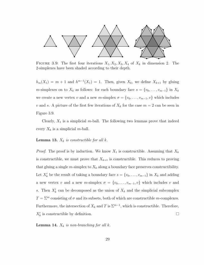
Figure 3.9: The first four iterations X1, X2, X3, X4 of Xk in dimension 2. The2-simplexes have been shaded according to their depth.
hm(X1) = m + 1 and hm−1(X1) = 1. Then, given Xk, we define Xk+1 by gluing
m-simplexes on to Xk as follows: for each boundary face s = {v0, . . . , vm−1} in Xk
we create a new vertex v and a new m-simplex σ = {v0, . . . , vm−1, v} which includes
v and s. A picture of the first few iterations of Xk for the case m = 2 can be seen in
Figure 3.9.
Clearly, X1 is a simplicial m-ball. The following two lemmas prove that indeed
every Xk is a simplicial m-ball.
Lemma 13. Xk is constructible for all k.
Proof. The proof is by induction. We know X1 is constructible. Assuming that Xk
is constructible, we must prove that Xk+1 is constructible. This reduces to proving
that gluing a single m-simplex to Xk along a boundary face preserves constructibility.
Let X ′k be the result of taking a boundary face s = {v0, . . . , vm−1} in Xk and adding
a new vertex v and a new m-simplex σ = {v0, . . . , vm−1, v} which includes v and
s. Then X ′k can be decomposed as the union of Xk and the simplicial subcomplex
T = Σm consisting of σ and its subsets, both of which are constructible m-complexes.
Furthermore, the intersection of Xk and T is Σm−1, which is constructible. Therefore,
X ′k is constructible by definition.
Lemma 14. Xk is non-branching for all k.
29

Proof. The proof is again by induction. We know that X1 is non-branching. Assume
this is true for Xk as well. By construction, s ∈ Sm−1(Xk) has another coface in
Sm(Xk+1) if and only if s has only one coface in Sm(Xk). The new (m−1)-simplexes
are the boundary faces of Xk+1 and thus have exactly one coface. Thus, the total
number of cofaces of every (m− 1)-simplex in Xk+1 is either one or two.
As mentioned in the introduction, constructible non-branching simplicial m-
complexes are simplicial m-balls. Thus, every Xk is a simplicial m-ball.
To prove part (1) of Proposition 12, we need to keep track of how the Cheeger
numbers hm−1(Xk) and hm(Xk) change with k. This is accomplished in the following
two lemmas.
Lemma 15. hm−1(Xk) = 1k
for all k.
Proof. By Lemma 6, hm−1(Xk) = 1rad(Xk)
. For k = 1, rad(X1) = 1. Now suppose
that rad(Xk) = k. We will prove that in passing from Xk to Xk+1, all m-simplexes
originally in Xk have their depth increased by exactly 1 (we already know the new
m-simplexes in Xk+1 have depth 1).
If τ ∈ Sm(Xk) has depth d and φ is a depth-attaining cochain for τ in Xk, then
φ is a sum of a sequence {si}di=1 of (m − 1)-simplexes satisfying the conditions in
Lemma 5. All of those conditions are preserved in going from Xk to Xk+1, except
that sd is no longer a boundary face. Instead, if sd = {v0, . . . , vm−1} then a new
vertex v and a new m-simplex σ = {v0, . . . , vm−1, v} are created which prevent sd
from being a boundary face and add σ to the coboundary of φ. However, if we add
any of the other faces of σ to φ (which are all boundary faces), we obtain a new
cochain φ′ with δφ′ = τ and ‖φ′‖ = d + 1. Thus, the depth of τ in Xk+1 is at most
d+ 1.
Conversely, if τ has depth d′ in Xk+1 and ψ =∑d′
i=1 ti is a depth-attaining
cochain for τ with {ti}d′i=1 satisfying the conditions in Lemma 5, then ψ′ =
∑d′−1i=1 ti
30

is a cochain in Xk with δψ′ = τ , so that the depth of σ is at most d′ − 1. Thus, if
τ has depth d in Xk then its depth in Xk+1 must be at least d + 1. Combined with
the above result we conclude that all m-simplexes originally in Xk have their depth
increased by exactly 1 in Xk+1.
Lemma 16. hm(Xk) ≥ m− 1 for all k.
Proof. We know that hm(X1) = m + 1 ≥ m − 1. Now suppose hm(Xk) ≥ m − 1.
Any chain φ ∈ Cm(Z2;Xk+1) attaining hm can be decomposed into a chain ψ ∈
Cm(Z2;Xk) plus a chain ψ′ which is a sum of depth 1 simplexes in Xk+1. Then we
can write ‖∂φ‖ = ‖∂ψ‖ + ‖∂ψ′‖ − 2x where x is the number of (m − 1)-simplexes
shared by ∂ψ and ∂ψ′. Since m of the m + 1 faces of any m-simplex in ψ′ are
boundary faces, x ≤ ‖ψ′‖. Also, it is clear that ‖∂ψ′‖ = (m+ 1)‖ψ′‖. Thus,
‖∂φ‖‖φ‖
=‖∂ψ‖+ (m+ 1)‖ψ′‖ − 2x
‖ψ‖+ ‖ψ′‖
≥ ‖∂ψ‖+ (m− 1)‖ψ′‖‖ψ‖+ ‖ψ′‖
≥ min
{‖∂ψ‖‖ψ‖
,m− 1
}≥ m− 1
(In fact, with some effort it can be seen that hm = (m+1)(m−1)(m+1)−2m−k+1 .)
By Theorem 8, λm−1(Xk) = λm(Xk) ≥ (m−1)2
2(m+1). This completes the proof of part
(1) of Proposition 12.
In order to define the family Yk we need to make use of the notion of stellar
subdivision, which can be traced back to at least Alexander (1930).
Definition 17 (Stellar Subdivision). Let Y be a simplicial m-complex and let σ =
{v0, . . . , vm} ∈ Sm(Y ). The stellar subdivision of Y along σ, denoted by sdσ Y , is
31

the simplicial m-complex obtained from Y by creating a new vertex w and replacing
σ with the m-simplexes
τi = {v0, . . . , vi−1, w, vi+1, . . . , vm}
where i = 0, . . . ,m. For notational purposes, we denote the j-th face of τi by ti,j :=
τi \ {vj} for i 6= j, and ti,i := τi \ {w}. If σ1, . . . , σn ∈ Sm(Y ), then we define the
stellar subdivision of Y along the σi to be
sdσ1,...,σn Y := sdσ1 sdσ2 · · · sdσn Y
We now define the Yk recursively. Let Σm be the simplicial complex induced
by a single m-simplex σ and let Y1 := sdσ Σm. Label the m-simplexes of Y1 as
σ0, . . . , σm and call their common vertex (the one created by stellar subdivision)
the central vertex v. Now, given a Yk containing the central vertex v, we call all
m-simplexes containing v the inner m-simplexes of Yk and label them as σ0, . . . , σn.
All non-inner m-simplexes will be referred to as outer m-simplexes. We then define
Yk+1 := sdσ0,...,σn Yk. Note that v and all outer m-simplexes (and the simplexes they
contain) are preserved unchanged in going from Yk to Yk+1 while all of the inner
m-simplexes are subdivided. Furthermore, it is clear that all the Yk are subdivisions
of Σm and are thus simplicial m-balls. A picture of the first few iterations of Yk for
m = 2 can be seen in Figure 3.10.
To prove part (2) of Proposition 12, we need to keep track of how the Cheeger
numbers hm−1(Yk) and hm(Yk) change with k. This is accomplished in the following
two lemmas.
Lemma 18. hm−1(Yk) ≥ 1k
for all k.
Proof. By Lemma 6, we can prove this by keeping track of the depths of all the
m-simplexes of Yk. For Y1, all the m-simplexes σi contain a boundary face (using the
32

Figure 3.10: The first three iterations Y1, Y2, Y3 of Yk in dimension 2. The 2-simplexes have been shaded according to their depth.
notation of Definition 17 with σi = τi, the boundary face of σi is ti,i). Thus, every
σi has depth 1 and by Lemma 6, hm−1(Y1) = 1. Note that the cochain φ which is
depth-attaining for some σi does not include any (m− 1)-simplex which contains v.
Now suppose for induction that every outer m-simplex σ of Yk has depth ≤ k
and a depth-attaining cochain φ ∈ Cm−1(Z2) such that φ does not contain any face
of any inner m-simplex. Then in Yk+1, φ remains unaltered, proving that σ still has
depth ≤ k in Yk+1.
Similarly, suppose that every inner m-simplex σ of Yk has depth ≤ k via a depth-
attaining cochain φ which does not contain any (m−1)-simplex containing v. Then in
Yk+1, σ is removed and replaced by new m-simplices. Using the notation of Definition
17, in Yk+1 the coboundary of φ becomes δφ = τm+1, so that the depth of τm+1 is
at most k. Furthermore, by adding any face t(m+1),j to φ (j 6= m + 1) we obtain a
cochain φ′ with δφ′ = τj, proving that the depth of τj is at most k + 1. Since φ′
still does not contain any (m − 1)-simplex which contains v, we are back where we
started. The statement now follows by induction.
Lemma 19. hm(Yk) ≤ 1mk−1 for all k > 1.
Proof. To prove this, we merely count the number of m-simplexes in Yk. Note that
33

in going from Yk to Yk+1 we replace (m+ 1)mk−1 inner m-simplexes with (m+ 1)mk
inner m-simplexes. Thus, Yk+1 has
(m+ 1)mk − (m+ 1)mk−1 = (m+ 1)(m− 1)mk−1
more m-simplexes than Yk. Since |Sm(Y1)| = m + 1, this means that |Sm(Yk)| is
equal to
(m+ 1) + (m+ 1)(m− 1) + (m+ 1)(m− 1)m+ . . .
+ (m+ 1)(m− 1)mk−2 = (m+ 1)mk−1.
Since Yk has m + 1 boundary faces, the chain φ containing all m-simplexes of Yk
gives the upper bound on hm(Yk):
hm(Yk) ≤‖∂φ‖‖φ‖
=m+ 1
(m+ 1)mk−1=
1
mk−1.
By Theorem 8, λm−1(Yk) = λm(Yk) ≤ 1mk−1 . This completes the proof of Propo-
sition 12.
3.3 Relation to Graphs
In Chung (2007), Fan Chung defines a normalized local Dirichlet Cheeger number
and normalized local Dirichlet eigenvalue and proves an inequality between them. If
one translates Fan Chung’s result to the unnormalized case for graphs with vertex
degree upper bounded by m+ 1, it closely resembles Theorem 8.
Translating Theorem 1 of Chung (2007) into the unnormalized setting, it reads
as follows. Given a graph G we can prescribe a certain set of vertices to be the
boundary vertices of the graph. Let S be the prescribed boundary vertex set, and
34
let
hS := hS(G) = min‖δφ‖‖φ‖
where the minimum is taken over all nonzero φ ∈ C0(Z2) such that φ does not include
any boundary vertex. Similarly, let
λS = min‖δf‖2
2
‖f‖22
where the minimum is taken over all nonzero f ∈ C0(R) such that f(s) = 0 for all
s ∈ S. We can also characterize λS as the smallest eigenvalue of LS0 , the submatrix
of L0 consisting of the rows and columns of L0 not indexed by vertices in S. In this
case, LS0 is a map on C0S(R), the subspace of C0(R) spanned by the vertices not in
S. Then if every vertex has degree upper bounded by m+ 1
hS ≥ λS ≥h2S
2(m+ 1).
To relate the above inequality to the simplicial complex setting, we note that for
every non-branching simplicial m-complex X, one can construct a graph G (similar
to the dual graph defined in Fomin et al. (2008)) as follows. Begin by constructing
the simplicial complex X ′ as in the proof of Theorem 8 and let S be the set of border
facets of X ′. Create a vertex in G for every m-simplex in X ′. We will use S to
denote both the border facets of X ′ and the set of vertices in G which correspond
the border facets. Connect two vertices with an edge whenever the corresponding
m-simplexes are lower adjacent in X ′. Since X ′ is non-branching, the vertices of
G have degree upper bounded by m + 1. Identifying C0S(G; R) with Cm(X; R), we
can ask if Lm : Cm(X; R) → Cm(X; R) and LS0 : C0S(G; R) → C0
S(G; R) are the
same map. They are the same if and only if X is orientable (this is easy to see
from the characterization of the Laplacian in Muhammad and Egerstedt (2006)). In
35

addition, hm(X) and hS are equal regardless of orientability. Thus, for non-branching
orientable simplicial m-complexes, Theorem 8 reduces to the result proved by Fan
Chung, and the proofs are identical. The difference is that Theorem 8 covers the
more general cases of non-orientable and branching simplicial m-complexes, for which
parts of the inequality may still hold.
The real projective plane provides a simple example of how orientation plays a
role in our analysis of the Cheeger inequality and why it doesn’t play a role in Chung
(2007). In Figure 3.11, the first image shows the fundamental polygon that defines
RP 2, the second image shows a triangulation X of RP 2, and the third image is
the dual graph G of the triangulation (in the second and third image, edges with
similar color are identified). In this simple example, there is no boundary (S = ∅).
In the triangulation, if one considers the 2-chain φ ∈ C2(Z2) which contains every
2-simplex, then ∂φ = 0 and thus h2(X) = 0. However, if one considers the 2-chain
f ∈ C2(X; R) that assigns a 1 to every 2-simplex with the orientation shown in the
figure, the boundary of f is a 1-chain which assigns a 2 to every colored edge with
the orientation shown. In particular, ∂f 6= 0 and in fact λ2 6= 0 as a result of the
nonorientability of RP 2. However, the dual graph cannot see this nonorientability,
as the 0-chain f ∈ C0S(G; R) corresponding to f has empty coboundary, meaning
λS = 0. Thus, in this case the map L2 is not the same as the map LS0 , and Theorem
1 of Chung (2007) still holds while part 1 of Theorem 8 fails.
3.4 Discussion and Open Problems
A result of the universal coefficient theorem in algebraic topology is that torsion will
be an obstacle in relating higher-dimensional Cheeger numbers with eigenvalues. The
Cheeger inequality for graphs holds without any assumptions since zeroth homology
is never affected by torsion. For higher dimensions either the inequality does not
hold or we require assumptions that remove torsion. The negative results for the
36

Figure 3.11: The fundamental polygon of RP 2, a triangulation, and the dual graphof the triangulation.
Cheeger inequality in Gundert and Wagner (2012) are for simplicial complexes with
torsion. Torsion is also known to affect algorithmic complexity. For example, the
problem of finding minimal weight cycles given a simplicial complex with weights is
NP-hard if there is torsion and is otherwise a linear program (see Dey et al. (2011)).
A local Cheeger number and algebraic connectivity for graphs with Dirichlet like
boundary conditions was defined in Chung (2007) and a Cheeger inequality was
proved. There is a close relation between Theorem 1 of Chung (2007) and Theorem
8. If Theorem 1 is adapted to an unnormalized setting (see section 3.3) then for
non-branching orientable simplicial m-complexes Theorem 8 reduces to Theorem 1.
However, Theorem 8 covers the more general cases of non-orientable and branching
simplicial m-complexes.
We close with a few open problems of possible interest.
1. Intermediate values of k – Given a simplicial m-complex, what can we say
about the relationship between hk and λk or hk and λk for 1 < k < m − 1?
Torsion again will need to be addressed but are there some conditions under
which some Cheeger-type inequalities may hold?
2. High-order eigenvalues – In Lee et al. (2011) the authors introduce higher-
order (as opposed to higher-dimensional) Cheeger numbers on the graph which
37
correspond to higher-order eigenvalues of the graph Laplacian and prove a
general Cheeger inequality for them. A natural question is how our results
would extend to higher-orders. Indeed, by analogy with the Rayleigh quotient
characterization of higher order eigenvalues, it would seem reasonable to define
the kth dimensional, jth order coboundary Cheeger numbers to be
hk,j := minφ∈Ck(Z2)φ/∈Sj
‖δφ‖minψ∈Sj
‖φ+ ψ‖
where
Sj = span(im δ ∪ {φ1, . . . , φj−1})
is the subspace of Ck(Z2) spanned by im δ and cochains φ1, . . . , φj−1 which at-
tain hk,1, . . . , hk,j−1, respectively. The higher order boundary Cheeger numbers
hk,j could be defined similarly. One would need to prove that this definition
makes sense and then ask whether they satisfy any inequalities with the corre-
sponding eigenvalues.
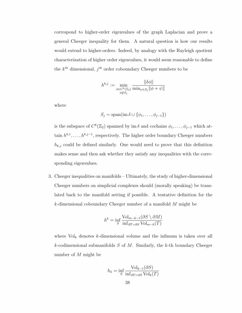
3. Cheeger inequalities on manifolds – Ultimately, the study of higher-dimensional
Cheeger numbers on simplicial complexes should (morally speaking) be trans-
lated back to the manifold setting if possible. A tentative definition for the
k-dimensional coboundary Cheeger number of a manifold M might be
hk = infS
Volm−k−1(∂S \ ∂M)
inf∂T=∂S Volm−k(T )
where Volk denotes k-dimensional volume and the infimum is taken over all
k-codimensional submanifolds S of M . Similarly, the k-th boundary Cheeger
number of M might be
hk = infS
Volk−1(∂S)
inf∂T=∂S Volk(T )
38

where again Volk denotes k-dimensional volume and the infimum is taken over
all k-dimensional submanifolds S of M .
39

4
Stochastic Methods in the Spectral Theory ofSimplicial Complexes
4.1 Introduction
4.1.1 Background
The relation between spectral graph theory and random walks on graphs has been
well studied and has both theoretical and practical implications (see Chung (1997);
Lovasz (1996); Meila and Shi (2001)). A classic example of this relation is graph
expansion (see Hoory et al. (2006)). Loosely speaking, graph expansion measures
how far a graph is from being disconnected (i.e., having a nontrivial reduced 0-th
homology class). The two common characterizations of graph expansion use either
the Cheeger number which relates to spectral graph theory or the mixing time of a
random walk on the graph.
In this chapter we examine an analagous relation between random walks on sim-
plicial complexes and spectral properties of higher order Laplacians. A simplicial
complex is a higher-dimensional generalization of a graph consisting of vertices and
edges as well as higher-dimensional simplices such as triangles and tetrahedra. The
40
graph Laplacian was generalized to simplicial complexes by Eckmann in Eckmann
(1945), resulting in what are called higher order combinatorial Laplacians. The k-th
order combinatorial Laplacian, or k-Laplacian, can be used to study expansion in the
sense that the spectrum of the k-Laplacian provides information on how far from the
complex is from having a nontrivial k-th (co)homology class. The graph Laplacian is
simply the 0-th order combinatorial Laplacian. There has been recent work extend-
ing Cheeger numbers and random walks to higher dimensions (see ?Lubotzky (2013);
Parzanchevski et al. (2012); Parzanchevski and Rosenthal (2012) and Chapter 3 of
this thesis).
The k-Laplacian is naturally decomposed into two parts commonly called the
up k-Laplacian and the down k-Laplacian. The graph case is an exception in that
there is only an up 0-Laplacian; the down 0-Laplacian is the zero matrix. This
fact suggests that a straightforward generalization of the theory of graph expansion
to higher dimensions may only relate to the up k-Laplacian. Indeed, the Cheeger
number of a graph was initially generalized so as to relate to the up k-Laplacian (see
?), with the generalization to the down k-Laplacian following soon after (see Chapter
3).
This decomposition also appears when studying random walks on simplicial com-
plexes. In a recent paper, Rosenthal and Parzanchevski generalized random walks on
graphs to random walks on simplicial complexes (see Parzanchevski and Rosenthal
(2012)). They defined a Markov chain on the space of oriented k-simplexes that
reflects the spectrum of the up k-Laplacian, assuming 0 ≤ k ≤ d− 1 where d is the
dimension of the simplicial complex. The walk traverses the simplicial complex by
moving between oriented k-simplexes via shared (k + 1)-simplexes. In this chapter
we define a random walk that traverses the simplicial complex by traveling through
shared (k − 1)-simplexes. We demonstrate that this random walk is related to the
spectrum of the down k-Laplacian and reflects the dimension of the k-th homology
41
group over R, assuming 1 ≤ k ≤ d. We also discuss the possibility of defining other
random walks on simplicial complexes, including random walks relating to the full
k-Laplacian and weighted Laplacians. We also apply random walks on simplicial
complexes to a semi-supervised learning problem, propagating oriented labels on
edges. This generalizes the method of label propagation on graphs to a new problem
in which the underlying structure to be learned is directional or is flow-like.
4.1.2 Motivation
We have two motivations for studying the random walk corresponding to the down
Laplacian. The first motivation comes from an example. Consider the 2-dimensional
simplicial complex formed by a hollow tetrahedron (or any triangulation of the 2-
sphere). We know that the complex has nontrivial 2-dimensional homology since
there is a void. However, this homology cannot be detected by the random walk
defined in Parzanchevski and Rosenthal (2012), because there are no tetrahedrons
that can be used by the walk to move between the triangles. In general, the walk
defined in Parzanchevski and Rosenthal (2012) can detect homology from dimension
0 to co-dimension 1, but never co-dimension 0. Hence, a new walk which can travel
from triangles to triangles through edges is needed.
The second motivation relates to the geometry of random walks or diffusions and
manifolds. The geometry captured by the graph Laplacian as well as the Cheeger
number and random walks on the graph have direct connections to the geometry of a
manifold with Neumann boundary conditions. We will examine random walks that
have connections to the geometry of a manifold with Dirichlet boundary conditions,
denoted as “Dirichlet” random walks. Work by Fan Chung in Chung (2007) has
shown that there are alternative notions of the Laplacian and random walks on graphs
that capture a Dirichlet-flavored geometry of graphs. The definition of the “local”
Cheeger number of a graph given in Chung (2007) bears a striking resemblance to the
42

definition of the Cheeger number of a manifold with Dirichlet boundary (see Cheeger
(1970)). Also defined in Chung (2007) is a “local” random walk that satisfies a
Dirichlet boundary condition. In contrast, the usual random walk on a graph might
be called Neumann. The random walk defined by Rosenthal and Parzanchevski
in Parzanchevski and Rosenthal (2012) generalizes the Neumann random walk to
higher dimensions on simplicial complexes. In this chapter we generalize the Dirichlet
random walk.
4.1.3 Summary of Results
In this section we give a short summary of the main results. Precise definitions of
the terms used are given in section 4.2.
In section 4.3 we define a p-lazy Dirichlet random walk on the oriented k-simplexes
of a d-dimensional simplicial complex X, where 1 ≤ k ≤ d. This walk has a cor-
responding probability transition matrix P . In most analyses of random walks the
questions of interest are convergence and rates of convergence of limn→∞ Pnν = π,
where ν is the initial probability distribution on the states, P nν is the marginal dis-
tribution after n steps of the walk, and π is the stationary or invariant distribution.
For the usual random walk on a graph, the graph Laplacian is used to study the lim-
iting behavoir of P nν. For the random walks we consider, orientation issues prevent
a straightforward connection between the k-Laplacian and P nν. Instead, we find a
connection between the k-Laplacian and CTP nν where C is a constant and T is a
linear transformation. The linear transformation T enforces antisymmetry between
the opposite orientations of a simplex. Denoting σ+ and σ− as the (arbitrarily cho-
sen) positive and negative orientations of a simplex σ, TP nν is a function on the set
of positively oriented simplexes such that
TP nν(σ+) = P nν(σ+)− P nν(σ−).
43

The constant C is a normalizing constant that ensures CTP nν has nontrivial limiting
behavior. Letting M denote the maximum number of k-simplexes any (k−1)-simplex
is contained in,
C =M − 1
p(M − 2) + 1.
Let 1τ denote the initial distribution supported on the oriented simplex τ and let
Eτn := CTP n1τ . The down k-Laplacian is Ldownk = δk−1∂k where δ is a coboundary
operator and ∂ is the boundary operator, and let λk denote the smallest eigenvalue
of Ldownk with eigenvector perpendicular to im ∂k+1. The following proposition is a
direct result of Theorem 30.
Proposition 20. If M−23M−4
< p < 1, then the limit Eτ∞ := limn→∞ Eτn exists for all
initial τ . In this case, the k-th homology group of X with coefficients in R is trivial
if and only if Eτ∞ ∈ im ∂k+1 for all τ . In addition, if p ≥ 12
then
‖Eτn − Eτ∞‖2 = O
([1− 1− p
(p(M − 2) + 1)(k + 1)λk
]n).
One difference in the above result with standard results on Markov chains is
that the limiting object provides information on the homology of X. This will be
discussed further in section 4.3. Another difference is that for a connected graph the
random walk is irreducible, and the limit distribution is independent of the initial
distribution. In higher dimensions, this independence is lost, even for complexes with
trivial k-th homology over R.
4.1.4 Related Work
The relation between graph random walks and the geometry of graphs has been
examined in both Dodziuk (1984) and Chung (2007). In section 4.6.1 we show
that under certain conditions the Dirichlet random walk in codimension 0 coincides
44
with the notion of a random walk on a graph with Dirichlet boundary. A natural
question to ask concerning random walks on simplicial complexes is: what would be
the analogous process on manifolds? In general we are not aware of results on the
continuum limit of these walks. However, the Dirichlet random walk in codimension
zero is analogous to the concept of Brownian motion with killing as described by
Lawler and Sokal in Lawler and Sokal (1988).
4.2 Definitions
In this section we define the simplicial complex X, the chain and cochain complexes,
and the k-Laplacian.
4.2.1 Simplicial Complexes
By a simplicial complex we mean an abstract finite simplicial complex. Simplicial
complexes generalize the notion of a graph to higher dimensions. Given a set of
vertices V , any nonempty subset σ ⊆ V of the form σ = {v0, v1, . . . , vj} is called a
j-dimensional simplex, or j-simplex. A simplicial complex X is a finite collection of
simplexes of various dimensions such that X is closed under inclusion, i.e., τ ⊆ σ and
σ ∈ X implies τ ∈ X. While we will not need it for this chapter, one can include the
empty set in X as well (thought of as a (−1)-simplex). Given a simplicial complex
X, denote the set of j-simplexes of X as Xj. We say that X is d-dimensional or
that X is a d-complex if Xd 6= ∅ but Xd+1 = ∅. Graphs are 1-dimensional simplicial
complexes. We will assume throughout that X is a d-complex for some fixed d ≥ 1.
If σ ∈ Xj and τ ∈ Xj−1 and τ ⊂ σ, then we call τ a face of σ and σ a coface
of τ . Every j-simplex has exactly j + 1 faces but may have any number of cofaces.
Given σ ∈ Xj we define deg(σ) (called the degree of σ) to be the number of cofaces
of σ. Two simplexes are upper adjacent if they share a coface and lower adjacent
if they share a face. The number of simplexes upper adjacent to a j-simplex σ is
45

(j+1)·deg(σ) while the number of simplexes lower adjacent to σ is∑
τ⊂σ(deg(τ)−1)
where the sum is over all faces τ of σ.
Orientation plays a major role in the geometry of a simplicial complex. For
j > 0, an orientation of a j-simplex σ is an equivalence class of orderings of its
vertices, where two orderings are equivalent if they differ by an even permutation.
Notationally, an orientation is denoted by placing one of its orderings in square
brackets, as in [v0, . . . , vj]. Every j-simplex σ has two orientations which we think of
as negatives of each other. We abbreviate these two orientations as σ+ and σ− = −σ+
(which orientation σ+ corresponds to is chosen arbitrarily). For j = 0 there are no
distinct orderings, but it is useful to think of each vertex v as being positively oriented
by default (so, v+ = v) and having an oppositely-oriented counterpart v− := −v. For
any j, we will use Xj+ = {σ+ : σ ∈ Xj} to denote a choice of positive orientation σ+
for each j-simplex σ. The set of all oriented j-simplexes will be denoted by Xj±, so
that Xj± = {σ± : σ+ ∈ Xj
+} and |Xj±| = 2|Xj| for any choice of orientation Xj
+.
An oriented simplex σ+ = [v0, . . . , vj] induces an orientation on the faces of σ as
(−1)i[v0, . . . , vi−1, vi+1, . . . , vj]. Conversely, an oriented face (−1)i[v0, . . . , vi−1, vi+1, . . . , vj]
of σ induces an orientation σ+ = [v0, . . . , vj] on σ. Two oriented j-simplexes σ+ and
σ′+ are said to be similarly oriented, and we write σ+ ∼ σ′+, if σ and σ′ are distinct,
lower adjacent j-simplexes and σ+ and σ′+ induce the opposite orientation on the
common face (if σ and σ′ are upper adjacent as well, this is the same as saying that
σ+ and σ′+ induce the same orientation on the common coface). If they induce the
same orientation on the common face, then we say they are dissimilarly oriented
and write σ− ∼ σ′+. We say that a d-complex X is orientable if there is a choice of
orientation Xd+ such that for every pair of lower adjacent simplexes σ, σ′ ∈ Xd, the
oriented simplexes σ+, σ′+ ∈ Xd
+ are similarly oriented.
46

4.2.2 Chain and Cochain Complexes
Given a simplicial complex X, we can define the chain and cochain complexes of
X over R. The space of j-chains Cj := Cj(X; R) is the vector space of linear
combinations of oriented j-simplexes with coefficients in R, with the stipulation that
the two orientations of a simplex are negatives of each other in Cj (as implied by our
notation). Thus, any choice of orientation Xj+ provides a basis for Cj. The space of
j-cochains Cj := Cj(X; R) is then defined to be the vector space dual to Cj. These
spaces are isomorphic and we will make no distinction between them. Usually, we will
work with cochains using the basis elements {1σ+ : σ+ ∈ Xj+}, where 1σ+ : Cj → R
is defined on a basis element τ+ ∈ Xj+ as
1σ+(τ+) =
{1 τ+ = σ+
0 else.
The boundary map ∂j : Cj → Cj−1 is the linear map defined on a basis element
[v0, . . . , vj] as
∂j[v0, . . . , vj] =
j∑i=0
(−1)i[v0, . . . , vi−1, vi+1, . . . , vj]
The coboundary map δj−1 : Cj−1 → Cj is then defined to be the transpose of the
boundary map. In particular, for f ∈ Cj−1,
(δj−1f)([v0, . . . , vj]) =
j∑i=1
(−1)if([v0, . . . , vi−1, vi+1, . . . , vj]).
When there is no confusion, we will denote the boundary and coboundary maps by
∂ and δ. It holds that ∂∂ = δδ = 0, so that (Cj, ∂j) and (Cj, δj) form chain and
cochain complexes.
47
The homology and cohomology vector spaces of X over R are
Hj := Hj(X; R) =ker ∂j
im ∂j+1
and Hj := Hj(X; R) =ker δj
im δj−1.
It is known from the universal coefficient theorem that Hj is the vector space dual
to Hj. Reduced (co)homology can also be used, and it is equivalent to including the
nullset as a (−1)-dimensional simplex in X.
4.2.3 The Laplacian
The k-Laplacian of X is defined to be
Lk := Lupk + Ldown
k
where
Lupk = ∂k+1δ
k and Ldownk = δk−1∂k.
The Laplacian is a symmetric positive semi-definite matrix, as is each part Lupk and
Ldownk . From Hodge theory, it is known that
kerLk ∼= Hk ∼= Hk
and the space of cochains decomposes as
Ck = im ∂k+1 ⊕ kerLk ⊕ im δk−1
where the orthogonal direct sum ⊕ is under the “usual” inner product
〈f, g〉 =∑
σ+∈Xk+
f(σ+)g(σ+).
We are interested in the Ldownj half of the Laplacian. Trivially, im ∂j+1 ⊆ kerLdown
j .
The smallest nontrivial eigenvalue of Ldownk is therefore given by
λk = minf∈Ck
f⊥im ∂
‖∂f‖22
‖f‖22
,
48

where ‖f‖2 :=√〈f, f〉 denotes the Euclidean norm on Ck. A cochain f that achieves
the minimum is an eigenvector of λk. It is easy to see that any such f is also an
eigenvector of Lk with eigenvalue λk and that, therefore, λk relates to homology:
λk = 0⇔ kerLk 6= 0⇔ Hk 6= 0.
Remark 21. Given a choice of orientation Xk+, Ldown
k can be written as a matrix with
rows and columns indexed by Xk+, the entries of which are given by
(Ldownk )σ′+,σ+
=
k + 1 σ′+ = σ+
1 σ′− ∼ σ+
−1 σ′+ ∼ σ+
0 else
.
Changing the choice of orientation Xk+ amounts to a change of basis for Ldown
k . If
the row and column indexed by σ+ are instead indexed by σ−, all the entries in them
switch sign except the diagonal entry. Alternatively, Ldownk can be characterized by
how it acts on cochains:
Ldownk f(τ+) = (k + 1) · f(τ+) +
∑σ−∼τ+
f(σ+)−∑σ+∼τ+
f(σ+).
Note that since Ldownk f is a cochain, Ldown
k f(τ−) = −Ldownk f(τ+).
The behavior of Ldownk is related to the following concepts:
Definition 22. A d-complex X is called k-connected (1 ≤ k ≤ d) if for every two
k-simplexes σ, σ′ there exists a chain σ = σ0, σ1, . . . , σn = σ′ of k-simplexes such that
σi is lower adjacent to σi+1 for all i. For a general d-complex X, such chains define
equivalence classes of k-simplexes, and the subcomplexes induced by these are called
the k-connected components of X.
Definition 23. A d-complex X is called disorientable if there is a choice of orienta-
tion Xd+ of its d-simplexes such that all lower adjacent d-simplexes are dissimilarly
oriented. In this case, the d-cochain f =∑
σ+∈Xd+1σ+ is called a disorientation.
49
Remark 24. Disorientability was defined in Parzanchevski and Rosenthal (2012) and
shown to be a higher-dimensional analogue of bipartiteness for graphs. Note that one
can also define X to be k-disorientable if the k-skeleton of X (the k-complex given
by the union⋃i≤kX
i) is disorientable, but this can only happen when k = d. This is
not hard to see: if k < d then there exists a (k+ 1)-simplex σ+ = [v0, . . . , vk]. Given
any two dissimilarly oriented faces of σ+, say, [v1, v2, . . . , vk] and [v0, v2, . . . , vk], we
find that the simplex {v0, v1, v3, . . . , vk} cannot be dissimilarly oriented to both of
them simultaneously.
Lemma 25. Let X be a d-complex, 1 ≤ k ≤ d and M = maxσ∈Xk−1 deg(σ).
1. Spec(Ldownk ) is the disjoint union of Spec(Ldown
k |Xi) where Xi are the k-connected
components of X.
2. The spectrum of Ldownk is contained in [0, (k + 1)M ].
3. The kernal of Ldownk is exactly ker ∂k = im ∂k+1 ⊕ kerLk.
4. The upper bound (k + 1)M is attained if and only if k = d and X has a d-
connected component that is both disorientable and of constant (d− 1)-degree.
Proof. Statement (1) follows from the fact that Ldownk can be written as a block
diagonal matrix with each block corresponding to a component Xi. Statement (3) is
easy to verify.
For statement (2), let f be an eigenvector of Ldownk with eigenvalue λ, let Xk
+ be
a choice of orientation such that f(σ+) ≥ 0 for all σ+ ∈ Xk+ and suppose f(τ+) =
50
maxσ+∈Xk+f(σ+). Then by Remark 21,
λf(τ+) = Ldownk f
= (k + 1) · f(τ+) +∑σ−∼τ+
f(σ+)−∑σ+∼τ+
f(σ+)
≤ (k + 1) · f(τ+) +∑σ−∼τ+
f(σ+) +∑σ+∼τ+
f(σ+)
≤ (k + 1) · f(τ+) +∑σ−∼τ+
f(τ+) +∑σ+∼τ+
f(τ+)
≤ (k + 1) · f(τ+) + (k + 1)(M − 1) · f(σ+)
≤ (k + 1)M · f(τ+)
where the third inequality results from the fact that any k-simplex is lower adjacent
to at most (k + 1)(M − 1) other k-simplexes. Therefore, λ ≤ (k + 1)M .
It now remains to prove statement (4). Looking back at the inequalities, it holds
that λ = (k + 1)M only if σ− ∼ τ+ and f(σ+) = f(τ+) whenever σ and τ are lower
adjacent, and the faces of σ all have degree M . But since f(σ+) = f(τ+), the same
reasoning can be applied to f(σ+) for all σ lower adjacent to τ and eventually to all
k-simplexes in the same k-connected component Xi. Ultimately, this implies that Xi
has constant (k − 1)-degree and is k-disorientable (and hence k = d).
To see that this bound is indeed attainable, consider a disorientable d-complex
with constant (d − 1)-degree M (this includes, for instance, the simplicial complex
induced by a single d-simplex). Let Xd+ be a choice of orientation such that all lower
adjacent d-simplexes are dissimilarly oriented. Then a disorientation f on Xd will
51

satisfy
Ldownk f(τ+) = (k + 1) · f(τ+) +
∑σ−∼τ+
f(σ+)−∑σ+∼τ+
f(σ+)
= (k + 1) · f(τ+) +∑σ−∼τ+
f(σ+)
= (k + 1) · 1 +∑σ−∼τ+
1
= (k + 1)M · 1 = (k + 1)M · f(τ+)
for every τ+.
4.3 Random walks and the k-Laplacian
In this section we define the p-lazy Dirichlet k-walk on X and relate this walk to the
spectrum of the k-Laplacian.
Random walks and Ldownk Let X be a d-complex, 1 ≤ k ≤ d, 0 ≤ p < 1, and
M = maxσ∈Xk−1 deg(σ).
Definition 26. The p-lazy Dirichlet k-walk on X is an absorbing Markov chain on
the state space S = Xk± ∪ {Θ} defined as follows:
• Let two oriented k-cells s, s′ ∈ Xk± be called textitneighbors (denoted s ∼ s′) if
they share a face and are similarly oriented. In what follows, Θ will be used
to represent an additional absorbing state, called the “death state”, that the
Markov chain can occupy.
• Starting at an initial oriented k-simplex τ+ ∈ Xk±, the walk proceeds as a time-
homogenous Markov chain on the state space S = Xk± ∪ {Θ} with transition
52

probabilities
Prob(σ+ → σ′+) = Prob(σ− → σ′−) =
p σ′+ = σ+
1−p(M−1)(k+1)
σ′+ ∼ σ+
0 else,
Prob(σ+ → σ′−) = Prob(σ− → σ′+) =
{1−p
(M−1)(k+1)σ′− ∼ σ+
0 else,
Prob(σ+ → Θ) = Prob(σ− → Θ) = 1−∑σ′+
Prob(σ+ → σ′+),
Prob(Θ→ Θ) = 1
for all σ, σ′ ∈ Xk.
• This walk can be interpreted as follows. Starting at τ+, the walk has probability
p of staying put and for each of the neighbors of τ+ the walk has probability
1−p(M−1)(k+1)
of jumping to that neighbor. Note that if the number of neighbors of
τ+ is less than (M−1)(k+1), then the sum of these probabilities is less than 1.
In this case, we interpret the difference as the probability that the walker dies
(i.e., the walker jumps to a death state from which it can never return). The
same holds for τ−.
The left stochastic matrix for the Markov chain is a square matrix P with rows
and columns indexed by the state space S = Xk± ∪ {Θ} such that
Ps1,s2 = Prob(s2 → s1)
for all s1, s2 ∈ S. In stochastic processes it is more common to use the right stochastic
matrix P T as the probability matrix, for us it will be more convenient to use the
left stochastic matrix. An initial distribution on the state space is a column vector
ν indexed by S such that all entries are non-negative and sum to 1. The general
53

framework in stochastic processes is to study how the marginal distribution P nν
evolves as n→∞. Indeed, one can view the Dirichlet k-walk as a Markov chain on
a graph with vertex set V = S and study the limiting behavior of P nν within the
context of graph theory. However, this is not our goal. Our goal is to connect the
k-walk to the k-dimensional Laplacian, and hence to the k-dimensional topology and
geometry of X.
In order to connect the k-walk to Lk, we will not study the evolution of P nν but
rather TP nν, the image of the marginal distribution under a linear transformation
T defined as follows. Given a choice of orientation Xk+ = {σ+ : σ ∈ Xk}, T is defined
to be the matrix with rows indexed by Xk+ and columns indexed by S such that
(T )σ+,σ+ = 1 and (T )σ+,σ− = −1
for all σ ∈ Xk, and such that all other entries are 0. In other words, for any function
f : S → R, Tf is the function Tf : Xk+ → R such that
Tf(σ+) = f(σ+)− f(σ−).
The definition of T is motivated by geometry. The geometry of simplicial complexes
is characterized by the space of k-cochains Ck in which σ+ = −σ− (and for which Xk+
is a choice of basis). Probabilistically, σ+ and σ− are completely separate states for
the Markov chain, but geometrically we must think of them as opposite orientations
of the same underlying object σ. In addition, the state Θ has no corresponding
object in Ck, so T simply removes it from the system. Of course, the vector TP nν
does not have the property that it is always a distribution (all entries nonnegative
and summing to 1), but it has the advantage that it resides in Ck and can be related
to Lk as follows.
Definition 27. The propagation matrix B of the Dirichlet k-walk is defined to be a
54
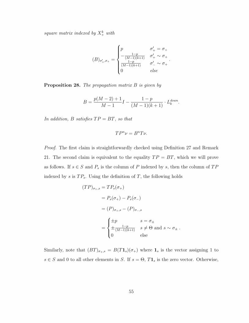
square matrix indexed by Xk+ with
(B)σ′+,σ+=
p σ′+ = σ+
− 1−p(M−1)(k+1)
σ′+ ∼ σ+
1−p(M−1)(k+1)
σ′− ∼ σ+
0 else
.
Proposition 28. The propagation matrix B is given by
B =p(M − 2) + 1
M − 1I − 1− p
(M − 1)(k + 1)· Ldown
k .
In addition, B satisfies TP = BT , so that
TP nν = BnTν.
Proof. The first claim is straightforwardly checked using Definition 27 and Remark
21. The second claim is equivalent to the equality TP = BT , which we will prove
as follows. If s ∈ S and Ps is the column of P indexed by s, then the column of TP
indexed by s is TPs. Using the definition of T , the following holds
(TP )σ+,s = TPs(σ+)
= Ps(σ+)− Ps(σ−)
= (P )σ+,s − (P )σ−,s
=
±p s = σ±
± 1−p(M−1)(k+1)
s 6= Θ and s ∼ σ±
0 else
.
Similarly, note that (BT )σ+,s = B(T1s)(σ+) where 1s is the vector assigning 1 to
s ∈ S and 0 to all other elements in S. If s = Θ, T1s is the zero vector. Otherwise,
55

if s = τ± then T1s = ±1τ+ and
(BT )σ+,s = ±B 1τ+(σ+)
= ±(B)σ+,τ+
=
±p τ+ = σ+
± 1−p(M−1)(k+1)
τ+ ∼ σ+
∓ 1−p(M−1)(k+1)
τ− ∼ σ+
0 else
=
±p s = σ±
± 1−p(M−1)(k+1)
s ∼ σ±
0 else
.
This concludes the proof.
For what follows, we define Eτ+n := Bn1τ+ to be the marginal difference of the
p-lazy Dirichlet k-walk on X starting at τ+. Also, let Xk+ be a choice of orientation
and denote M = maxσ∈Xk−1 deg(σ).
Corollary 29.
1. The spectrum of B is contained in[2p− 1, p(M−2)+1
M−1
], with the upper bound
acheived by cochains in ker ∂k and the lower bound acheived if and only if k = d
and there is a disorientable d-connected component of constant (d− 1)-degree.
2. If τ has a coface, then
‖Eτ+n ‖2 ≥(p(M − 2) + 1
M − 1
)n1√k + 2
.
3. If p 6= 0, 1 then
‖Eτ+n ‖2 ≤ max
{|2p− 1|n,
(p(M − 2) + 1
M − 1
)n}.
56

Proof. Statement (1) is easy to verify with the help of Lemma 25 and Proposition 28.
Statement (3) follows from the inequality ‖Af‖2 ≤ ‖A‖‖f‖2 where A is a matrix, f
is a vector, and ‖A‖ is the spectral norm on A.
It remains now to prove statement (2). If τ has a coface σ, let f = ∂k+11σ+ (with
σ+ being any orientation of σ) so that f ∈ ker ∂k. Let f, f1, . . . , fi be an orthogonal
basis for Ck such that f1, . . . , fi are eigenvectors of B with eigenvalues γ1, . . . , γi, and
assume 1τ+ = αf + α1f1 + . . .+ αi, fi. Then,
‖Eτ+n ‖2 = ‖Bn1τ+‖2 (4.1)
= ‖αBnf + α1Bnf1 + . . .+ αiB
nfi‖2 (4.2)
= |α|(p(M − 2) + 1
M − 1
)n‖f‖2 + |α1|γn1 ‖f1‖2 + . . .+ |αi|γni ‖fi‖2 (4.3)
≥ |α|(p(M − 2) + 1
M − 1
)n‖f‖2 (4.4)
=
(p(M − 2) + 1
M − 1
)n ∣∣∣∣⟨ f
‖f‖2
,1τ+
⟩∣∣∣∣ (4.5)
=
(p(M − 2) + 1
M − 1
)n |f(τ+)|‖f‖2
(4.6)
=
(p(M − 2) + 1
M − 1
)n1√k + 2
(4.7)
Note that if p 6= 0, 1, then |2p − 1| and p(M−2)+1M−1
are both less than one. Hence,
the above corollary says that the limit of the marginal difference is trivial in general.
We can remove this trivial behavior by making one final alteration to our object
of study: multiply the propagation matrix B by M−1p(M−2)+1
to obtain the normalized
propagation matrix B := M−1p(M−2)+1
B and define Eτ+n := Bn1τ+ to be the normalized
marginal difference. The next two theorems show that the homology of X can be
determined from the limiting behavior of the normalized marginal difference.
57

Theorem 30.
The limit Eτ+∞ := limn→∞ Eτ+n of the normalized marginal difference exists for all τ+ if
and only if B has no eigenvalue λ ≤ −1. Furthermore, Eτ+∞ = projker ∂k1τ+ whenever
Eτ+∞ exists, where projker ∂kis the projection map onto ker ∂k.
Proof. Note that by Corollary 29, the spectrum of B is upper bounded by 1 and the
eigenspace of the eigenvalue 1 is exactly ker ∂k. Let f1, . . . , fi be an orthogonal basis
for Ck such that f1, . . . , fi are eigenvectors of B with eigenvalues γ1, . . . , γi. Then
any 1τ+ can be written as a linear combination 1τ+ = α1f1 + . . .+ αi, fi so that
Eτ+∞ = Bn1τ+ = α1γn1 f1 + . . . , αiγ
ni fi
Since the fj form a basis, Eτ+∞ converges if and only if αjγnj converges for each j. In
other words, Eτ+∞ converges if and only if for every j, αj = 0 or γj > −1. Furthermore,
the limit (when it exists) is always
∑{j:γj=1}
αjfj = projker ∂k1τ+
Finally, suppose B has an eigenvalue λ ≤ −1. Then there is an eigenvector f
such that Bnf = λnf does not converge. Since the set of cochains {1τ+ : τ+ ∈ Xk±}
spans Ck(R), f can be written as a linear combination of them and therefore Bn1τ+
must not converge for some τ+.
Theorem 31.
1. If M−23M−4
< p < 1 then the limit Eτ+∞ exists for all τ+ and
dim(span{projker δk Eτ+∞ : τ+ ∈ Xk±}) = dim(Hk(X))
where projker δk denotes the projection map onto ker δk.
58
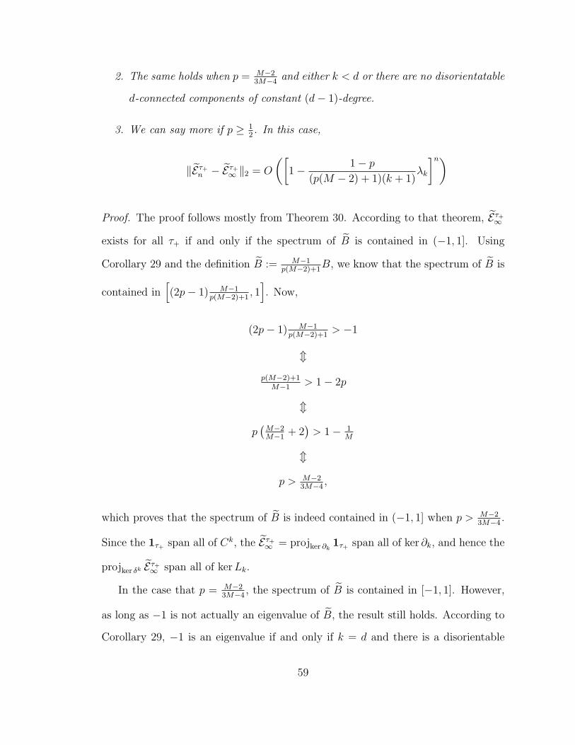
2. The same holds when p = M−23M−4
and either k < d or there are no disorientatable
d-connected components of constant (d− 1)-degree.
3. We can say more if p ≥ 12. In this case,
‖Eτ+n − Eτ+∞ ‖2 = O
([1− 1− p
(p(M − 2) + 1)(k + 1)λk
]n)
Proof. The proof follows mostly from Theorem 30. According to that theorem, Eτ+∞
exists for all τ+ if and only if the spectrum of B is contained in (−1, 1]. Using
Corollary 29 and the definition B := M−1p(M−2)+1
B, we know that the spectrum of B is
contained in[(2p− 1) M−1
p(M−2)+1, 1]. Now,
(2p− 1) M−1p(M−2)+1
> −1
m
p(M−2)+1M−1
> 1− 2p
m
p(M−2M−1
+ 2)> 1− 1
M
m
p > M−23M−4
,
which proves that the spectrum of B is indeed contained in (−1, 1] when p > M−23M−4
.
Since the 1τ+ span all of Ck, the Eτ+∞ = projker ∂k1τ+ span all of ker ∂k, and hence the
projker δk Eτ+∞ span all of kerLk.
In the case that p = M−23M−4
, the spectrum of B is contained in [−1, 1]. However,
as long as −1 is not actually an eigenvalue of B, the result still holds. According to
Corollary 29, −1 is an eigenvalue if and only if k = d and there is a disorientable
59
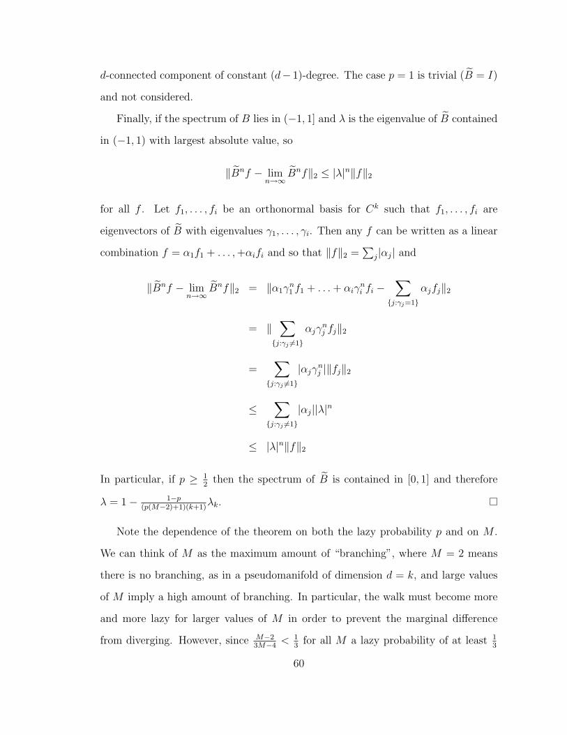
d-connected component of constant (d− 1)-degree. The case p = 1 is trivial (B = I)
and not considered.
Finally, if the spectrum of B lies in (−1, 1] and λ is the eigenvalue of B contained
in (−1, 1) with largest absolute value, so
‖Bnf − limn→∞
Bnf‖2 ≤ |λ|n‖f‖2
for all f . Let f1, . . . , fi be an orthonormal basis for Ck such that f1, . . . , fi are
eigenvectors of B with eigenvalues γ1, . . . , γi. Then any f can be written as a linear
combination f = α1f1 + . . . ,+αifi and so that ‖f‖2 =∑
j|αj| and
‖Bnf − limn→∞
Bnf‖2 = ‖α1γn1 f1 + . . .+ αiγ
ni fi −
∑{j:γj=1}
αjfj‖2
= ‖∑{j:γj 6=1}
αjγnj fj‖2
=∑{j:γj 6=1}
|αjγnj |‖fj‖2
≤∑{j:γj 6=1}
|αj||λ|n
≤ |λ|n‖f‖2
In particular, if p ≥ 12
then the spectrum of B is contained in [0, 1] and therefore
λ = 1− 1−p(p(M−2)+1)(k+1)
λk.
Note the dependence of the theorem on both the lazy probability p and on M .
We can think of M as the maximum amount of “branching”, where M = 2 means
there is no branching, as in a pseudomanifold of dimension d = k, and large values
of M imply a high amount of branching. In particular, the walk must become more
and more lazy for larger values of M in order to prevent the marginal difference
from diverging. However, since M−23M−4
< 13
for all M a lazy probability of at least 13
60

will always ensure convergence. While there is no explicit dependence on k or the
dimension d, it is easy to see that M must always be at least d− k+ 1 (for instance,
it is not possible for a triangle complex to have maximum vertex degree 1).
We would also like to know whether for the normalized marginal difference con-
verges to 0. Note that if τ+ has a coface, then we already know that ‖Eτ+n ‖2 stays
bounded away from 0 according to Corollary 29. However, if τ has no coface, then
1τ+ may be perpendicular to ker ∂k, allowing ‖Eτ+n ‖2 to die in the limit as we see in
the following corollary.
Corollary 32. If τ has no coface, Hk = 0, and if M−23M−4
< p < 1 then
‖Eτ+∞ ‖2 = 0.
The same is true when p = M−23M−4
and either k < d or there are no disorientable
d-connected components of constant (d− 1)-degree,
Proof. Under all conditions stated, Eτ+∞ converges. If τ has no coface, then 1τ+ is in
the orthogonal complement of im ∂k+1, because all elements of im ∂k+1 are supported
on oriented faces of (k + 1)-simplexes. If Hk = 0 then ker ∂k = im ∂k+1, so that
‖Eτ+∞ ‖2 = projker ∂k1τ+ = 0.
4.4 Random walks with Neumann boundary conditions
The Neumann random walk described by Rosenthal and Parzanchevski in Parzanchevski
and Rosenthal (2012) is the “dual” of the Dirichlet random walk, jumping from
simplex to simplex through cofaces rather than faces. Let X be a d-complex,
0 ≤ k ≤ d− 1, and 0 ≤ p < 1.
61

Definition 33. The p-lazy Neumann k-walk on X is an absorbing markov chain on
the state space S = Xk± ∪ {Θ} defined as follows:
• Let two oriented k-simplexes s, s′ ∈ Xk± be called coneighbors (denoted s _ s′)
if they share a coface and are dissimilarly oriented. Also, let deg(σ) denote the
number of cofaces of σ. In what follows, Θ is an additional absorbing state the
random walk can occupy, called the “death state”.
• Starting at an initial oriented k-simplex τ+ ∈ Xk± the walk proceeds as a time-
homogeneous Markov chain on S := Xk± ∪ {Θ} with transition probabilities
Prob(σ+ → σ′+) = Prob(σ− → σ′−) =
p σ′+ = σ+
1−pk·deg(σ)
σ′+ _ σ+
0 else,
Prob(σ+ → σ′−) = Prob(σ− → σ′+) =
{1−p
k·deg(σ)σ′− _ σ+
0 else,
Prob(σ+ → Θ) = Prob(σ− → Θ) =
{1− p deg(σ) = 0
0 else,
Prob(Θ→ Θ) = 1.
for all σ, σ′ ∈ Xk.
• This walk can be described as follows. Starting at at any σ+, the walk has a
probability p of staying put and otherwise is equally likely to jump to one of the
k ·deg(σ) coneighbors of σ+. If σ has no coneighbors (i.e., if σ has no cofaces),
then the walk instead has probability p of staying put and probability 1 − p of
jumping to the absorbing state Θ. The same holds for starting at σ−.
62

This definition varies from that in Parzanchevski and Rosenthal (2012) where
the case of k = d − 1 was examined and it was assumed that every k-simplex had
at least one coface, and as a result a death state was not required. The inclusion
of the death state in all cases in the definition above allows us to use the matrix
T from Section 4.3 to relate the marginal distribution of the walk to Lupk . If ν is
an initial distribution and P is the left stochastic matrix for the walk (so that P nν
is the marginal distribution after n steps), then TP nν is the marginal difference
after n steps for the Neumann k-walk. Similar to the Dirichlet walk, there is a
propagation matrix A such that TP nν = AnTν and such that A relates to Lupk .
Once again the marginal difference converges to 0 for all initial distributions, but this
behavior is fixed by multiplying A by a constant, obtaining a normalized propagation
matrix A and a normalized marginal distribution AnTν. The limiting behavior of
the normalized marginal difference reveals homology similar to Theorem 31.
While the results for the Neumann and Dirichlet walks are quite similar, we
highlight two differences. One is that the norm of the normalized marginal difference
for the Neumann k-walk starting at a single oriented simplex stays bounded away
from 0 (see Proposition 2.8 of Parzanchevski and Rosenthal (2012)), whereas this
need not hold for the Dirichlet k-walk (as in Corollary 32). This is because in the
Neumann case, every starting point 1τ+ has some nonzero inner product with an
element of im δk−1 ⊆ ker δk. The second difference is in the threshold values for p in
Theorem 31 and in the corresponding Theorem 2.9 of Parzanchevski and Rosenthal
(2012). For the Dirichlet walk, homology can be detected for p > M−23M−4
(where
M = maxσ∈Xk−1 deg(σ)) whereas for the Neumann walk the threshold is p > k3k+2
.
Hence, the Neumann walk is sensitive to the dimension while the Dirichlet walk is
sensitive to the maximum degree. In both cases, p ≥ 13
is always sufficient to detect
homology and p ≥ 12
allows us to put a bound on the rate of convergence.
63
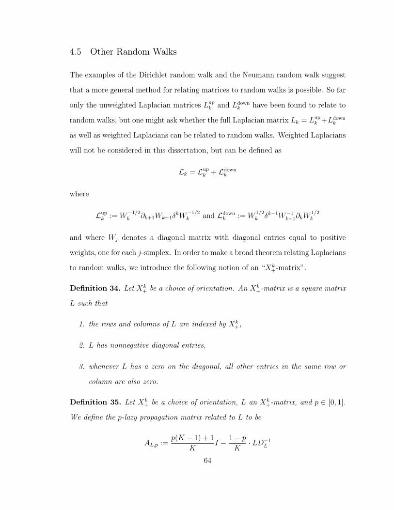
4.5 Other Random Walks
The examples of the Dirichlet random walk and the Neumann random walk suggest
that a more general method for relating matrices to random walks is possible. So far
only the unweighted Laplacian matrices Lupk and Ldown
k have been found to relate to
random walks, but one might ask whether the full Laplacian matrix Lk = Lupk +Ldown
k
as well as weighted Laplacians can be related to random walks. Weighted Laplacians
will not be considered in this dissertation, but can be defined as
Lk = Lupk + Ldown
k
where
Lupk := W
−1/2k ∂k+1Wk+1δ
kW−1/2k and Ldown
k := W1/2k δk−1W−1
k−1∂kW1/2k
and where Wj denotes a diagonal matrix with diagonal entries equal to positive
weights, one for each j-simplex. In order to make a broad theorem relating Laplacians
to random walks, we introduce the following notion of an “Xk+-matrix”.
Definition 34. Let Xk+ be a choice of orientation. An Xk
+-matrix is a square matrix
L such that
1. the rows and columns of L are indexed by Xk+,
2. L has nonnegative diagonal entries,
3. whenever L has a zero on the diagonal, all other entries in the same row or
column are also zero.
Definition 35. Let Xk+ be a choice of orientation, L an Xk
+-matrix, and p ∈ [0, 1].
We define the p-lazy propagation matrix related to L to be
AL,p :=p(K − 1) + 1
KI − 1− p
K· LD−1
L
64
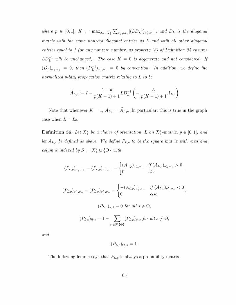
where p ∈ [0, 1], K := maxσ+∈Xk+
∑σ′+ 6=σ+
|(LD−1L )σ′+,σ+
|, and DL is the diagonal
matrix with the same nonzero diagonal entries as L and with all other diagonal
entries equal to 1 (or any nonzero number, as property (3) of Definition 34 ensures
LD−1L will be unchanged). The case K = 0 is degenerate and not considered. If
(DL)σ+,σ+ = 0, then (D−1L )σ+,σ+ = 0 by convention. In addition, we define the
normalized p-lazy propagation matrix relating to L to be
AL,p := I − 1− pp(K − 1) + 1
LD−1L
(=
K
p(K − 1) + 1AL,p
)
Note that whenever K = 1, AL,p = AL,p. In particular, this is true in the graph
case when L = L0.
Definition 36. Let Xk+ be a choice of orientation, L an Xk
+-matrix, p ∈ [0, 1], and
let AL,p be defined as above. We define PL,p to be the square matrix with rows and
columns indexed by S := Xk+ ∪ {Θ} with
(PL,p)σ′+,σ+= (PL,p)σ′−,σ− =
{(AL,p)σ′+,σ+
if (AL,p)σ′+,σ+> 0
0 else,
(PL,p)σ′−,σ+= (PL,p)σ′+,σ− =
{−(AL,p)σ′+,σ+
if (AL,p)σ′+,σ+< 0
0 else,
(PL,p)s,Θ = 0 for all s 6= Θ,
(PL,p)Θ,s = 1−∑
s′∈S\{Θ}
(PL,p)s′,s for all s 6= Θ,
and
(PL,p)Θ,Θ = 1.
The following lemma says that PL,p is always a probability matrix.
65

Lemma 37. Let Xk+ be a choice of orientation, L an Xk
+-matrix, and p ∈ [0, 1]. The
matrix PL,p defined above is the left stochastic matrix for an absorbing Markov chain
on the state space S (i.e., (PL)s′,s = Prob(s→ s′)) such that Θ is an absorbing state
and Prob(s→ s) = p for all s 6= Θ.
Proof. It is clear by the definition of PL,p that Θ is an absorbing state. To see that
Prob(s→ s) = p for all s 6= Θ, note that
(AL,p)σ+,σ+ =p(K − 1) + 1
K− 1− p
K· 1
=p(K − 1) + 1− 1 + p
K= p
and hence by the definition of PL,p,
(PL,p)σ−,σ− = (PL,p)σ+,σ+ = p
for all σ. It is also clear by the definition of PL,p that the entries (PL,p)σ′−,σ+=
(PL,p)σ′+,σ− are nonnegative for any σ, σ′. Hence, in order to show that PL,p is left
stochastic we need only to prove that∑
s′∈S\{Θ}(PL,p)s′,s ≤ 1 for all s ∈ S \ {Θ}. By
the symmetries inherent in PL,p, the value of the sum is the same for s = σ+ as it is
for s = σ−. For any s = σ+,∑s′∈S\{Θ}
(PL,p)s′,s =∑
σ′+∈Xk+
(AL,p)σ′+,σ+
= p+∑
σ′+∈Xk+\{σ+}
|(AL,p)σ′+,σ+|
= p+1− pK
∑σ′+∈Xk
+\{σ+}
|(LD−1L )σ′+,σ+
|
≤ p+ (1− p) = 1.
This completes the proof.
66

We will call PL,p the p-lazy probability matrix related to L. The following theorem
shows that PL,p is related L.
Theorem 38. Let Xk+ be a choice of orientation, L an Xk
+-matrix, p ∈ [0, 1], and
let AL,p and PL,p be defined as above. In addition, let T+ be defined as in section 4.3.
Then
AL,pT = TPL,p.
In other words, the evolution of the marginal differences T+PnL,pν after n steps with
initial distribution ν is governed by the propagation matrix: TP nL,pν = AnL,pTν.
Proof. Using the definition of T
(TPL,p)σ+,s = (PL,p)σ+,s − (PL,p)σ−,s
=
{±(AL,p)σ+,σ′+
s = σ′±0 s = Θ
.
Similarly, note that (AL,pT )σ+,s = AL,p(T1s)(σ+) where 1s is the vector assigning 1
to s ∈ S and 0 to all other elements in S. If s = Θ, T1s is the zero vector. Otherwise,
if s = τ± then T1s = ±1τ+ . Thus,
(AL,pT )σ+,s =
{±AL,p1τ+(σ+) s = τ±
0 s = Θ
=
{±(AL,p)σ+,τ+ s = τ±
0 s = Θ.
This concludes the proof.
Finally, we conclude with a few results motivating the normalized propagation
matrix and showing how the limiting behavior of the marginal difference relates to
the kernel and spectrum of L. We strongly suspect stronger results hold.
Theorem 39. Let Xk+ be a choice of orientation, L an Xk
+-matrix with Spec(L) ⊂
[0,Λ] (Λ > 0). Then for Λ−1K+Λ−1
≤ p < 1 the following statements hold:
67

1. ‖AnL,pTν‖2 → 0 for every initial distribution ν,
2. AnL,pTν → projkerLD−1 Tν for every initial distribution ν, where projkerL de-
notes the projection map onto the kernel of L,
3. If λ is the spectral gap (smallest nonzero eigenvalue) of L then
‖AnL,pTν − projkerL Tν‖2 = O
([1− 1− p
p(K − 1) + 1λ
]n).
Proof. The proof is the same as in the proofs of Corollary 29 and Theorem 31 and
mostly boil down to statements about the spectra of AL,p and AL,p. Note that since
Λ−1K+Λ−1
≤ p < 1, Spec(AL,p) ⊂ [0, 1] where the eigenspace of the eigenvalue 1 is equal
to the kernel of L, and the largest eigenvalue of AL,p less than 1 is 1− 1−pp(K−1)+1
λ.
As an example of the applicability of this framework, AL,p is used with L = Lk
to perform label propagation on edges in the next section.
4.6 Examples of random walks
In this section we state some specific random walks to provide some intuition for
random walks on complexes and to use the ideas we have developed to study a
problem in machine learning, semi-supervised learning.
4.6.1 Triangle complexes
We begin by reviewing local random walks on graphs as defined by Fan Chung in
Chung (2007). Given a graph G = (V,E) and a designated “boundary” subset
S ⊂ V , a 12-lazy random walk on S = V \S can be defined which satisfies a Dirichlet
boundary condition on S (meaning a walker is killed whenever it reaches S). The
walker starts on a vertex v0 ∈ S and at each step remains in place with probability
12
or else jumps to one of the adjacent vertices with equal probability. The boundary
68

condition is enforced by declaring that whenever the walker would jump to a vertex
in S, the walk ends. Thus, the left stochastic matrix P for this walk can be written
down as
(P )v′,v∈S = Prob(v → v′) =
12
if v = v′
12dv
if v ∼ v′
0 else
where v ∼ v′ denotes that vertices v and v′ are adjacent and dv is the number of edges
connected to v. Note that P is indexed only by S, and that its columns sums may
be less than 1. The probability of dying is implicitly encoded in P as the difference
between the column sum and 1. As was shown in Chung (2007), P is related to
a local Laplace operator also indexed by S. If D is the degree matrix and A the
adjacency matrix, the graph Laplacian of G is L = D − A. We denote the local
Laplacian as LS, where S in subscript means rows and columns indexed by S have
been deleted. The relation between P and LS is
P = I − 1
2LSD
−1S .
Hence, the existence and rate of convergence to a stationary distributions can be
studied in terms of the spectrum of the local Laplace operator.
Now suppose we are given an orientable 2-dimensional non-branching simplicial
complex X = (V,E, T ) where T is the set of triangles (subsets of V of size 3). Non-
branching means that every edge is contained in at most 2 triangles. We can define
a random walk on triangles fundamentally identical to a local walk on a graph which
reveals the 2-dimensional homology of X. The 12-lazy Dirichlet 2-walk on T starts
at a triangle t0 and at each step remains in place with probability 12
or else jumps to
the other side of one of the three edges. If no triangle lies on the other side of the
69
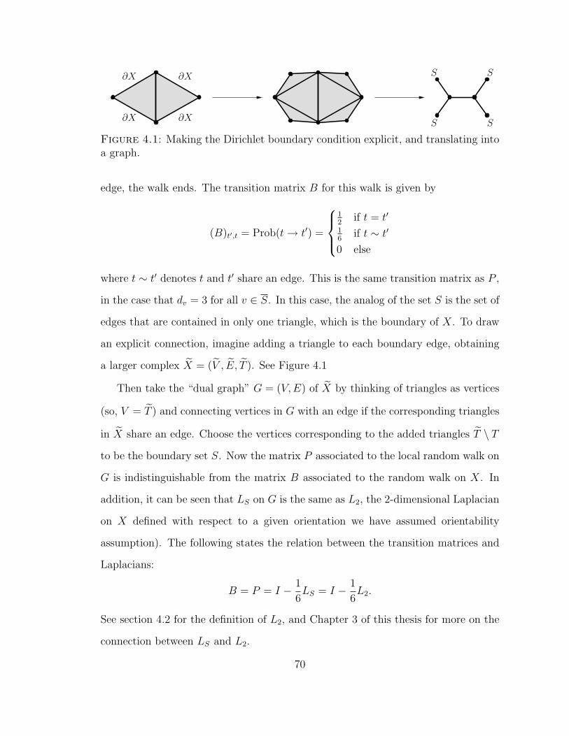
∂X
∂X
S
∂X S
∂X
S
S
Figure 4.1: Making the Dirichlet boundary condition explicit, and translating intoa graph.
edge, the walk ends. The transition matrix B for this walk is given by
(B)t′,t = Prob(t→ t′) =
12
if t = t′
16
if t ∼ t′
0 else
where t ∼ t′ denotes t and t′ share an edge. This is the same transition matrix as P ,
in the case that dv = 3 for all v ∈ S. In this case, the analog of the set S is the set of
edges that are contained in only one triangle, which is the boundary of X. To draw
an explicit connection, imagine adding a triangle to each boundary edge, obtaining
a larger complex X = (V , E, T ). See Figure 4.1
Then take the “dual graph” G = (V,E) of X by thinking of triangles as vertices
(so, V = T ) and connecting vertices in G with an edge if the corresponding triangles
in X share an edge. Choose the vertices corresponding to the added triangles T \ T
to be the boundary set S. Now the matrix P associated to the local random walk on
G is indistinguishable from the matrix B associated to the random walk on X. In
addition, it can be seen that LS on G is the same as L2, the 2-dimensional Laplacian
on X defined with respect to a given orientation we have assumed orientability
assumption). The following states the relation between the transition matrices and
Laplacians:
B = P = I − 1
6LS = I − 1
6L2.
See section 4.2 for the definition of L2, and Chapter 3 of this thesis for more on the
connection between LS and L2.
70

It is a basic fact that the kernel of L2 corresponds to the 2-dimensional homology
group of X over R. Therefore, there exists a stationary distribution for the random
walk if and only if X has nontrivial homology in dimension 2. Additionally, the rate
of convergence to the stationary distribution (if it exists) is governed by the spectral
gap of L2. In particular, the following statements hold:
1. Given a starting triangle t0, the marginal distribution of the random walk
after n steps is E t0n := Bn1t0 where 1t0 is the vector assigning a 1 to t0 and
0 to all other triangles. For any t0, the marginal distrubition converges, i.e.,
E t0∞ := limn→∞ E t0n exists.
2. The limit E t0∞ is equal to 0 for all starting triangles t0 if and only if X has trivial
homology in dimension 2 over R.
3. The rate of convergence is given by
‖E t0n − E t0∞‖2 = O
([1− 1
6λ2
]n)
where λ2 is the smallest nonzero eigenvalue of L2.
The example given here is constrained by certain assumptions (orientability and
the non-branching property), which allows for the most direct interpretation with
respect to previous work done on graphs.
4.6.2 Label propagation on edges
In machine learning random walks on graphs have been used for semi-supervised
learning. In this section we will generalize a class of algorithms on graphs called “label
propogation” algorithms to simplicial complexes, specifically we extend the algorithm
described in Zhu et al. (2005) (for more examples, see Callut et al. (2008); Jaakkola
and Szummer (2002); Zhou and Scholkopf (2004)). The goal of semi-supervised
71

classification learning is to classify a set of unlabelled objects {v1, . . . , vu}, given a
small set of labelled objects {vu+1, . . . , vu+`} and a set E of pairs of objects {vi, vj}
that one believes a priori to share the same class. Let G = (V,E) be the graph
with vertex set V = {v1, . . . , vu+`} and let P be the probability matrix for the usual
random walk, i.e.,
(P )ij = Prob(vj → vi) =1
dj
where dj is the degree of vertex j. We denote the classes an object belongs to as
c = 1, ..., C and an initial distribution f c0 : V → [0, 1] is the a priori confidence that
each vertex is in class c, a recursive label propagation process proceeds as follows.
1. For t = 1, ..., T and c = 1, .., C:
(a) Set f ct ← Pf ct−1
(b) Reset f ct (vi) = 1 for all vi labelled as c.
2. Consider f cT as an estimate of the relative confidence that each object is in class
c.
3. For each unlabelled point vi, i ≤ u, assign the label
arg maxc=1,..C
{f cT (vi)}.
The number of steps T is set to be large enough such that f cT is close to its limit
f c∞ := limT→∞ fcT . If G is connected, it can be shown that f c∞ is independent of the
choice of f c0 . Even if G is disconnected, the algorithm can be performed on each
connected component separately and again the limit f c∞ for each component will be
independent of the choice of f c0 .
We will now adapt the label propagation algorithm to higher dimensional walks,
namely, walks on oriented edges. Given any random walk on the set of oriented
72

edges (and an absorbing death state Θ), its probability transition matrix P could be
used to propagate labels in the same manner as the above algorithm. However, this
will treat and label the two orientations of a single edge separately as though they
are unrelated. As found in this chapter and in Parzanchevski and Rosenthal (2012),
geometric meaning and interesting long-term behavior is obtained by transforming
and normalizing P into a normalized propagation matrix, and applying it not to
functions on the state space but to 1-cochains. In this way we will infer only one label
per edge. One major change, however, is that labels will become oriented themselves.
That is, given an oriented edge e+ and a class c, the propagation algorithm may
assign a positive confidence that e+ belongs to class c or a negative confidence that
e+ belongs to class c, which we view as a positive confidence that e+ belongs to class
−c or, equivalently, that e− belongs to class c. This construction applies to systems
in which every class has two built-in orientations or signs, or the class information
has a directed sense of “flow”.
For example, imagine water flowing along a triangle complex in two dimensions.
Given an oriented edge, the water may flow in the positive or negative direction along
the edge. A “negative” flow of water in the direction of e+ can be interpreted as a
positive flow in the direction of e−. Perhaps the flow along a few edges is observed
and one wishes to infer the direction of the flow along all the other edges. Unlike in
the graph case, a single class of flow already presents a classification challenge. Or
consider multiple streams of water colored according to the C classes, we may want
to know which stream dominates the flow along each edge and in which direction. In
order to make these inferences, it is necessary to make some assumption about how
labels should propagate from one edge to the next. When considering water flow, it
is intuitive to make the following two assumptions.
1. Local Consistency of Motion. If water is flowing along an oriented edge
73

[vi, vj] in the positive direction, then for every triangle [vi, vj, vk] the water
should also tend to flow along [vi, vk] and [vk, vj] in the positive directions.
2. Preservation of Mass. The total amount of flow into and out of each vertex
(along edges connected to the vertex) should be the same.
In fact, either one of these assumptions is sufficient to infer oriented class labels
given the observed flow on a few edges. Depending on which assumptions one chooses,
different normalized propagation matrices AL,p (see section 4.5) may be applied.
For example, L = Lup1 will enforce local consistency of motion without regard to
preservation of mass, while L = Ldown1 will do the opposite. A reasonable way of
preserving both assumptions is by using L = L1 as shown in Example 42.
We now state a simple algorithm, analogous to the one for graphs, that propagates
labels on edges to infer a partially-observed flow. Let X be a simplicial complex of
dimension d ≥ 1 and let X1+ = {e1, . . . , en} be a choice of orientation for the set of
edges. Without loss of generality, assume that oriented edges eu + 1, . . . , en=u+` have
been classified with class c (not −c). Similar to the graph case, we apply a recursive
label propagation process to an initial distribution vector f c0 : X1+ → R measuring
the a priori confidence that each oriented edge is in class c. See Algorithm 1 for the
procedure. The result of the algorithm is a set of estimates of the relative confidence
that each edge is in class c with some orientation.
After running the algorithm, an unlabelled edge ei is assigned the oriented class
sgn(f cT (ei))c where c = arg maxc=1,..C{|f cT (ei)|}. We now prove that given enough
iterations T the algorithm converges and the resulting assigned labels are meaningful.
The proof uses the same methods as the one found in Zhu et al. (2005) for the graph
case.
Proposition 40. Using the notation of section 4.5, assume that L is a symmetric
Xk+-matrix with Spec(LD−1
L ) ⊂ [0,Λ]. Let AL,p be the normalized p-lazy propagation
74

Algorithm 1: Edge propagtion algorithm.
Data: Simplicial complex X, set of oriented edges
X1+ = {e1, . . . , eu, eu+1, ..., eu+`}
with eu+1, . . . , eu+` labelled with oriented classes ±1, ..,±C, initialdistribution vector f c0 : X1
+ → R, number of iterations TResult: Confidence of class membership and direction for unlabelled edges
{f c∗(e1), ..., f c∗(eu)}Cc=1
for c = 1 to C dofor t = 1 to T do
f ct ← AL,pfct−1;
f ct (ei)← 1 for ei labelled with class c;f ct (ei)← −1 for ei labelled with class −c
end
end
{f c∗(e1), ..., f c∗(eu)}Cc=1 ← {f cT (e1), ..., f cT (eu)}Cc=1;
matrix as defined in Definition 35. If Λ−22K+Λ−2
< p < 1 and if no vector in kerL is
supported on the set of unclassified edges, then Algorithm 1 converges. That is,
limT→∞
f cT =: f c∞ =
(ψc
(I − A4)−1A3ψc
),
where A4 and A3 are submatrices of AL,p and ψc is the class function on edges
labelled with ±c (for which ψc(ei) = ±1). In addition, f c∞ depends neither on the
initial distribution f c0 nor on the lazy probability p.
Proof. First, note that we are only interested in the convergence of f cT (ei) for ei not
labelled ±c. Partition f cT and AL,p according to whether ei is labelled ±c or not as
f cT =
(ψc
f cT
)and AL,p =
(A1 A2
A3 A4
).
The recursive definition of f cT in Algorithm 1 can now be rewritten as f cT = A4fcT−1 +
A3ψc. Solving for f cT in terms of f c0 yields
f cT = (A4)kf c0 +T−1∑i=0
(A4)iA3ψc.
75

In order to prove convergence of f cT , it suffices to prove that A4 has only eigenval-
ues strictly less than 1 in absolute value. This ensures that (A4)kf c0 converges to
zero (eliminating dependence on the initial distribution) and that∑k−1
i=0 (A4)iA3ψc
converges to (I − A4)−1A3ψc as k → ∞. We will prove that Spec(A4) ⊂ (−1, 1) by
relating Spec(A4) to Spec(LD−1L ) ⊂ [0,Λ] as follows.
First, partition L and DL similar to AL,p as
L =
(L1 L2
L3 L4
)and DL =
(D1 00 D4
).
so that
A4 = I − 1− pp(K − 1) + 1
L4D−14 .
Hence Spec(A4) is determined by Spec(L4D−14 ), or to be more specific, λ ∈ Spec(L4D
−14 )⇔
1 − 1−pp(K−1)+1
λ ∈ Spec(A4). Furthermore, note that L4D−14 and D
−1/24 L4D
−1/24 are
similar matrices and share the same spectrum. It turns out that the spectrum of
D−1/24 L4D
−1/24 is bounded within the spectrum of D
−1/2L LD
−1/2L , which in turn is
equal to Spec(LD−1L ) ⊂ [0,Λ] by similarity. Let g be an eigenvector of D
−1/24 L4D
−1/24
with eigenvalue λ and let g1, . . . , gj be an orthonormal basis of eigenvectors of
D−1/2L LD
−1/2L (such a basis exists since it is a symmetric matrix) with eigenvalues
µ1, . . . , µj. We can write
(0cg
)= α1g1 + . . .+ αjgj
for some α1, . . . , αj, where 0c is the vector of zeros with length equal to the number
76

of edges classified as ±c. Then
α1µ1g1 + . . .+ αjµjgj = D−1/2L LD
−1/2L
(0cg
)
=
(D−1/21 L1D
−1/21 D
−1/21 L2D
−1/24
D−1/24 L3D
−1/21 D
−1/24 L4D
−1/24
)(0cg
)
=
(D−1/21 L2D
−1/24 g
D−1/24 L4D
−1/24 g
)
=
(D−1/21 L2D
−1/24 g
λg
).
Taking the Euclidean norm of the beginning and ending expressions, we see that
|α1µ1|+ . . .+ |αjµj| = ‖(D−1/21 L2D
−1/24 g
λg
)‖2
≥ ‖λg‖2
= λ(|α1|+ . . .+ |αj|).
Because we assumed that µi ∈ [0,Λ] for all i, it would be a contradiction if λ < 0
or λ > Λ. The case λ = 0 is possible if and only if there is a vector in kerL that is
supported on the unlabelled edges. To see this, note that if λ = 0 then
α21µ1 + . . .+ α2
jµj =
(0cg
)TD−1/21 L2D
−1/24
(0cg
)
=
(0cg
)T (D−1/21 L2D
−1/24 g
λg
)= 0
which implies αiµi = 0 for all i and therefore(
0cg
)∈ kerL. Finally, since we
assumed that no vector in kerL is supported on the unlabelled edges and that
Λ−22K+Λ−2
< p < 1, we conclude that Spec(L4D−14 ) ⊂ (0,Λ] and therefore Spec(A4) ⊂[
1− 1−pp(K−1)+1
Λ, 1)⊂ (−1, 1).
77
To see that the solution f c∞ = (I − A4)−1A3ψc does not depend on p, note that
I −A4 is a submatrix of 1−pp(K−1)+1
LD−1L so that p(K−1)+1
1−p (I −A4) does not depend on
p. Then write f c∞ as
f c∞ =
[p(K − 1) + 1
1− p(I − A4)
]−1
× 1
1− pA3ψ
c
and note that p(K−1)+11−p A3 is an off-diagonal submatrix of p(K−1)+1
1−p I − LD−1L and
therefore does not depend on p either.
Note that while the limit f c∞ exists, the matrix I − A4 could be ill-conditioned.
In practice, it may be better to approximate f c∞ with f ct for large enough t. Also,
the algorithm will converge faster for smaller values of p and if f c0 = 0.
4.6.3 Experiments
We use some simulations to illustrate how Algorithm 1 works.
Example 41. Figure 4.2 shows a simplicial complex in which a single oriented edge
e1 has been labelled with class c (indicated by the red color) and all other edges
are unlabelled. Figure 4.3 shows what happens when this single label is propagated
T = 100 steps using Algorithm 1 with L = Lup1 , p = 0.9, and with f c0 equal to
the indicator function on e1. After the T steps have been performed the edges are
oriented and labelled according to the sign of f ck (if f ck(ei) = 0 for an oriented edge
ei, then that edge is left unoriented and unlabelled in the figure). Figures 4.4 and 4.5
show the same thing with L = Ldown1 and L = L1, respectively. The results using Lup
1
and Ldown1 have a clear resemblance to magnetic fields. When L = Ldown
1 , “mass” is
preserved which creates multiple vortices where the flow spins around a triangle. The
walk using Lup1 tries to maintain local consistency of motion, creating sources and
sinks in the process. The full L1 walk strikes somewhat of a balance between the two,
resulting in a more circular flow with a single vortex in the lower left.
78

Figure 4.2: A 2-complex with a labelled edge.
Figure 4.3: Label propagation with L = Lup1 .
Example 42. Figure 4.6 shows a simplicial complex in which two edges have been
labelled with class c = 1 (indicated by the red color) and two more edges have been
labelled with class c = 2 (indicated by the blue color). Figure 4.7 shows what happens
when the labels are propagated T = 1000 steps using Algorithm 1 with L = L1,
p = 0.9, and f c0 equal to the indicator function on the oriented edges labelled with
classes c = 1, 2. Every edge is then oriented and labelled according to the sign of
f c=1T , if |f c=1
T | > |f c=2T |, or f c=2
T , if |f c=1T | < |f c=2
T |. Notice that only a small number
of labels are needed to induce large-scale circular motion. Near the middle, a few
79

Figure 4.4: Label propagation with L = Ldown1 .
Figure 4.5: Label propagation with L = L1.
blue labels mix in with the red due to the asymmetry of the initial labels.
4.7 Discussion
In this chapter, we introduced a random walk with absorbing states on simplicial com-
plexes. Given a simplicial complex of dimension d, the relation between the random
walk and the spectrum of the k-dimensional Laplacian for 1 ≤ k ≤ d was examined.
We compared the Dirichlet random walk we introduced to the Neumann random
80

Figure 4.6: A 2-complex with two different labels on four edges.
Figure 4.7: Label propagation with L = L1.
81

walk introduced by Rosenthal and Parzanchevski in Parzanchevski and Rosenthal
(2012).
There remain many open questions about random walks on simplicial complexes
and the spectral theory of higher order Laplacians. Possible future directions of
research include:
(1) Is there a Brownian process on a manifold that corresponds to the continuum
limit of these new random walks?
(2) Is it possible to use conditioning techniques from stochastic processes such as
Doob’s h-transform to analyze these walks?
(3) What applications do these walks have to problems in machine learning and
statistics?
82

Bibliography
Alexander, J. W. (1930), “The combinatorial theory of complexes,” Ann. of Math.(2), 31, 292–320.
Alon, N. (1986), “Eigenvalues and expanders,” Combinatorica, 6, 83–96, Theory ofcomputing (Singer Island, Fla., 1984).
Alon, N. and Milman, V. D. (1985), “λ1, isoperimetric inequalities for graphs, andsuperconcentrators,” J. Combin. Theory Ser. B, 38, 73–88.
Bjorner, A. (1995), “Topological methods,” in Handbook of combinatorics, Vol. 1, 2,pp. 1819–1872, Elsevier, Amsterdam.
Buser, P. (1980), “On Cheeger’s inequality λ1 ≥ h2/4,” in Geometry of the Laplaceoperator (Proc. Sympos. Pure Math., Univ. Hawaii, Honolulu, Hawaii, 1979),Proc. Sympos. Pure Math., XXXVI, pp. 29–77, Amer. Math. Soc., Providence,R.I.
Callut, J., Francoisse, K., Saerens, M., and Dupont, P. (2008), “Semi-supervised clas-sification from discriminative random walks,” in Machine Learning and KnowledgeDiscovery in Databases, pp. 162–177, Springer.
Cheeger, J. (1970), “A lower bound for the smallest eigenvalue of the Laplacian,” inProblems in analysis (Papers dedicated to Salomon Bochner, 1969), pp. 195–199,Princeton Univ. Press, Princeton, N. J.
Chung, F. (2007), “Random walks and local cuts in graphs,” Linear Algebra Appl.,423, 22–32.
Chung, F. R. K. (1997), Spectral graph theory, vol. 92 of CBMS Regional ConferenceSeries in Mathematics, Published for the Conference Board of the MathematicalSciences, Washington, DC.
Dey, T. K., Hirani, A. N., and Krishnamoorthy, B. (2011), “Optimal homologouscycles, total unimodularity, and linear programming,” SIAM J. Comput., 40, 1026–1044.
83

Dodziuk, J. (1984), “Difference equations, isoperimetric inequality and transience ofcertain random walks,” Transactions of the American Mathematical Society, 284,787–794.
Dotterrer, D. and Kahle, M. (2012), “Coboundary expanders,” J. Topol. Anal., 4,499–514.
Eckmann, B. (1945), “Harmonische Funktionen und Randwertaufgaben in einemKomplex,” Comment. Math. Helv., 17, 240–255.
Fiedler, M. (1973), “Algebraic connectivity of graphs,” Czechoslovak Math. J.,23(98), 298–305.
Fomin, S., Shapiro, M., and Thurston, D. (2008), “Cluster algebras and triangulatedsurfaces. I. Cluster complexes,” Acta Math., 201, 83–146.
Guerini, P. and Savo, A. (2003), “The Hodge Laplacian on manifolds with boundary,”Seminaire de Theorie Spectrale et Geometrie (Univ. Grenoble I, Saint-Martin-d?Heres), 21, 125–146.
Gundert, A. and Wagner, U. (2012), “On Laplacians of random complexes,” in Com-putational geometry (SCG’12), pp. 151–160, New York, ACM.
Hoory, S., Linial, N., and Wigderson, A. (2006), “Expander graphs and their appli-cations,” Bull. Amer. Math. Soc. (N.S.), 43, 439–561 (electronic).
Jaakkola, T. and Szummer, M. (2002), “Partially labeled classification with Markovrandom walks,” Advances in Neural Information Processing Systems (NIPS), 14,945–952.
Lawler, G. F. and Sokal, A. D. (1988), “Bounds on the L2 spectrum for Markovchains and Markov processes: a generalization of Cheeger’s inequality,” Trans.Amer. Math. Soc., 309, 557–580.
Lee, J., Gharan, S., and Trevisan, L. (2011), “Multi-way spectral partitioning andhigher-order Cheeger inequalities,” Arxiv preprint arXiv:1111.1055.
Linial, N. and Meshulam, R. (2006), “Homological connectivity of random 2-complexes,” Combinatorica, 26, 475–487.
Lovasz, L. (1996), “Random walks on graphs: a survey,” in Combinatorics, PaulErdos is eighty, Vol. 2 (Keszthely, 1993), vol. 2 of Bolyai Soc. Math. Stud., pp.353–397, Janos Bolyai Math. Soc., Budapest.
Lubotzky, A. (2013), “Ramanujan Complexes and High Dimensional Expanders,”arXiv preprint arXiv:1301.1028.
84
Meila, M. and Shi, J. (2001), “A Random Walks View of Spectral Segmentation,” inAI and STATISTICS (AISTATS) 2001.
Meshulam, R. and Wallach, N. (2009), “Homological connectivity of random k-dimensional complexes,” Random Structures Algorithms, 34, 408–417.
Mohar, B. (1989), “Isoperimetric numbers of graphs,” Journal of Combinatorial The-ory, Series B, 47, 274–291.
Muhammad, A. and Egerstedt, M. (2006), “Control using higher order Laplaciansin network topologies,” in Proceedings of the 17th International Symposium onMathematical Theory of Networks and Systems, Kyoto, Japan, pp. 1024–1038.
Parzanchevski, O. and Rosenthal, R. (2012), “Simplicial complexes: spectrum, ho-mology and random walks,” arXiv preprint arXiv:1211.6775.
Parzanchevski, O., Rosenthal, R., and Tessler, R. J. (2012), “Isoperimetric Inequal-ities in Simplicial Complexes,” arXiv preprint arXiv:1207.0638.
Zhou, D. and Scholkopf, B. (2004), “Learning from labeled and unlabeled data usingrandom walks,” in Pattern Recognition, pp. 237–244, Springer.
Zhu, X., Lafferty, J., and Rosenfeld, R. (2005), “Semi-supervised learning withgraphs,” Ph.D. thesis, Carnegie Mellon University, Language Technologies Insti-tute, School of Computer Science.
85
Biography
The author, John Joseph Steenbergen, was born on July 29, 1985 in Indianapolis,
IN. John received a B.S. in Math (Honors) and a B.S. in Statistics from Purdue
University in May 2008, a M.S. in Mathematics from Duke University in December
2010, and a PhD in Mathematics from Duke University in December 2013. John held
a Duke Endowment fellowship to support his graduate studies at Duke University
from the fall of 2008 up until the fall of 2012. He expects to be working as a
Research Assistant Professor at the Mathematics, Statistics, and Computer Science
department of the University of Illinois at Chicago in the spring semester of 2014.
86
Related Documents


![M obius transform, moment-angle complexes and Halperin ...masuda/transformation36_2009/Lu.pdf · Let [m] = f1;:::;mg. {Abstract simplicial complexes on [m] An abstract simplicial](https://static.cupdf.com/doc/110x72/5f9eaee417f28c7b9f3f1f95/m-obius-transform-moment-angle-complexes-and-halperin-masudatransformation362009lupdf.jpg)


![Discrete Morse Theory on Simplicial Complexes · 2009-10-11 · Discrete Morse Theory on Simplicial Complexes August 27, 2009 ALEX ZORN ABSTRACT: Following [2] and [3], we introduce](https://static.cupdf.com/doc/110x72/5f11185967aa9a7a70707781/discrete-morse-theory-on-simplicial-complexes-2009-10-11-discrete-morse-theory.jpg)

