Toward the characterization of upper tropospheric clouds using Atmospheric Infrared Sounder and Microwave Limb Sounder observations

Toward the characterization of upper tropospheric clouds using

Atmospheric Infrared Sounder and Microwave Limb

Sounder observations

Brian H. Kahn,1 Annmarie Eldering,1 Amy J. Braverman,1 Eric J. Fetzer,1

Jonathan H. Jiang,1 Evan Fishbein,1 and Dong L. Wu1

Received 22 March 2006; revised 11 October 2006; accepted 19 October 2006; published 1 March 2007.

[1] We estimate the accuracy of cloud top altitude (Z) retrievals from the AtmosphericInfrared Sounder (AIRS) and Advanced Microwave Sounding Unit (AMSU) observingsuite (ZA) on board the Earth Observing System Aqua platform. We compare ZA withcoincident measurements of Z derived from the micropulse lidar and millimeter wavecloud radar at the Atmospheric Radiation Measurement (ARM) program sites ofNauru and Manus islands (ZARM) and the inferred Z from vertically resolved MicrowaveLimb Sounder (MLS) ice water content (IWC) retrievals. The mean difference in ZA

minus ZARM plus or minus one standard deviation ranges from �2.2 to 1.6 km ± 1.0 to4.2 km for all cases of AIRS effective cloud fraction (fA) > 0.15 at Manus Island using thecloud radar only. The range of mean values results from using different approaches todetermine ZARM, day/night differences, and the magnitude of fA; the variation about themean decreases for increasing values of fA. Analysis of ZARM from the micropulse lidarat Nauru Island for cases restricted to 0.05 � fA � 0.15 indicates a statistically significantimprovement in ZA � ZARM over the cloud radar-derived values at Manus Island. Inthese cases the ZA � ZARM difference is �1.1 to 2.1 km ± 3.0 to 4.5 km. These resultsimply that the operational ZA is quantitatively useful for constraining cirrus altitudedespite the nominal 45 km horizontal resolution. Mean differences of cloud top pressure(PCLD) inferred from coincident AIRS and MLS ice water content (IWC) retrievals dependupon the method of defining AIRS PCLD (as with the ARM comparisons) over theMLS spatial scale, the peak altitude and maximum value of MLS IWC, and fA. AIRS andMLS yield similar vertical frequency distributions when comparisons are limited tofA > 0.1 and IWC > 1.0 mg m�3. Therefore the agreement depends upon the opacity ofthe cloud, with decreased agreement for optically tenuous clouds. Further, the meandifference and standard deviation of AIRS and MLS PCLD are highly dependent on theMLS tangent altitude. For MLS tangent altitudes greater than 146 hPa, the strength of thelimb technique, the disagreement becomes statistically significant. This implies thatAIRS and MLS ‘‘agree’’ in a statistical sense at lower tangent altitudes and ‘‘disagree’’ athigher tangent altitudes. These results provide important insights on upper troposphericcloudiness as observed by nadir-viewing AIRS and limb-viewing MLS.

Citation: Kahn, B. H., A. Eldering, A. J. Braverman, E. J. Fetzer, J. H. Jiang, E. Fishbein, and D. L. Wu (2007), Toward the

characterization of upper tropospheric clouds using Atmospheric Infrared Sounder and Microwave Limb Sounder observations,

J. Geophys. Res., 112, D05202, doi:10.1029/2006JD007336.

1. Introduction

[2] Validating satellite cloud observations is made chal-lenging by spatial and temporal cloud variability at scalessimilar to and smaller than the satellite measurement.Historically, satellite derived cloud quantities have beencompared to ground-based measurements. Recently, a setof satellite instruments flying in formation, dubbed the

‘‘A-Train,’’ provides a unique opportunity to cross validatecloud measurements made from different angles and plat-forms with close coincidence. A high-quality record ofupper tropospheric cloudiness will lead toward an improvedunderstanding of atmospheric hydrological processes,atmospheric transport in the tropopause region, and the roleof cloudiness in Earth’s present and future climate[Intergovernmental Panel on Climate Change, 2001].[3] Much effort over the years has been spent on the cross

comparison of cloud observations from in situ, airborne,spaceborne and surface-based instrumentation. Thisincludes intercomparisons of satellite-retrieved cloud prop-

JOURNAL OF GEOPHYSICAL RESEARCH, VOL. 112, D05202, doi:10.1029/2006JD007336, 2007ClickHere

for

FullArticle

1Jet Propulsion Laboratory, Pasadena, California, USA.

Copyright 2007 by the American Geophysical Union.0148-0227/07/2006JD007336$09.00

D05202 1 of 15

erties to surface-based active measurements [e.g., Smith andPlatt, 1978; Vanbauce et al., 2003; Berendes et al., 2004;Hollars et al., 2004; Naud et al., 2004; Elouragini et al.,2005; Hawkinson et al., 2005; Mace et al., 2005], retrievalsfrom multiple satellite platforms [e.g., Stubenrauch et al.,1999, 2005; Wylie and Wang, 1999; Naud et al., 2002;Mahesh et al., 2004], satellite to aircraft platforms [e.g.,Sherwood et al., 2004], and multiple instruments collocatedon single and multiple aircraft platforms [e.g., Smith andFrey, 1990; Frey et al., 1999; Holz et al., 2006].[4] In situ measurements of cloud vertical location,

particle size distribution, ice particle habit, extinctioncoefficient, water phase, and ice and liquid water contentare critically important for independently validatingremote sensing-derived cloud quantities [Heymsfield andMcFarquhar, 2002]. However, cross comparing satellite-derived cloud quantities is equally important for assessingconsistency over global atmospheric conditions, as well asfor algorithmic and product improvements. The crosscomparison of cloud quantities is a more difficult problemthan the comparison of other fields, such as temperature andwater vapor [Fetzer et al., 2006; Gettelman et al., 2006],because of the greater variability of clouds on short tempo-ral and spatial scales.[5] One of the more important physical quantities required

for cloud-related research is cloud height [Cooper et al.,2003]. Active measurements, including the millimeter wavecloud radar and micropulse lidar located at the AtmosphericRadiation Measurement (ARM) program sites [Ackermanand Stokes, 2003], the Geoscience Laser Altimeter System(GLAS) located on board the Ice, Cloud, and Land ElevationSatellite (ICESat) [Spinhirne et al., 2005], and the CloudSat[Stephens et al., 2002] and Cloud-Aerosol Lidar and InfraredPathfinder Satellite Observations (CALIPSO) [Winker et al.,2003] missions, provide accurate and precise cloud base andheight information across a wide range of cloud opticalthickness, but at horizontal scales of a few hundred metersand for a limited number of locations. Satellite-based passiveobservations measure cloud properties at scales fromhundreds of meters to hundreds of kilometers and have dailyglobal coverage. Aircraft-based remote sensing observationsand in situ measurements of ice cloud properties have highspatial and temporal resolution but also have the smallestspatial and temporal coverage; these data will not be used inthis analysis.[6] Among the satellite-based cloud height observations,

those derived from passive infrared (IR) are the moreuncertain, but have the greatest global coverage and longesttime span. These satellite products must be compared withmore precise and accurate active lidar and radar-derivedmeasurements for nonopaque clouds. In addition, the Aquasatellite provides a unique opportunity to intercomparesimultaneous satellite-based cloud products from an IRimager, the Moderate Resolution Imaging Spectroradiometer(MODIS) [King et al., 1992], and an IR/microwave (MW)sounder suite, the Atmospheric Infrared Sounder (AIRS)[Aumann et al., 2003]/Advanced Microwave SoundingUnit (AMSU) with ground-based upward looking radarand lidar measurements at the Tropical West Pacific ARMsites. This comparison is especially important because theVisible Infrared Imager/Radiometer Suite (VIIRS) onfuture operational platforms, i.e., the National Polar-orbiting

Operational Environmental Satellite System (NPOESS) andNPOESS Preparatory Program (NPP), will not have theMODIS 15 mm channels, and cloud height products mayhave to be derived in combination with the onboard Cross-track Infrared Sounder (CrIS)/Advanced TechnologyMicrowave Sounder (ATMS) Sounder Suite (CrIMMS)[Cunningham and Haas, 2004].[7] Cloud height is derived from IR CO2 temperature

sounding channels, used in a technique called ‘‘CO2 slic-ing’’ [Smith and Platt, 1978, and references therein; Menzelet al., 1983] where calculated radiances from an operationalweather forecast model are differenced with observed radi-ances, and the height is derived from ratios of the differ-ences. The largest error sources from CO2 slicing includethose from the calculated radiances that have error contri-butions from spectroscopic parameters, and others that areneeded to calculate radiances, like surface emissivity, andtemperature and water vapor profiles. These errors areespecially large near the surface but could affect cloudproducts several kilometers above the surface because ofthe relatively broad weighting functions of the MODIStemperature-sounding channels. In general, the CO2 slicingmethod is most accurate for high and opaque clouds, withincreasing degradation in accuracy as cloud height andopacity decrease [Wielicki and Coakley, 1981]. Other stud-ies have shown that an improvement in CO2 slicing-derivedcloud top height (Z) is observed when accounting forsurface emissivity effects over land [Zhang and Menzel,2002]; however, multilevel cloud cover was shown [Baumand Wielicki, 1994] to introduce errors in Z. More recentwork by Holz et al. [2006] suggests that sorting CO2 slicingchannels by optical depth to determine optimal channelpairs using high spectral resolution measurements improvesZ retrievals for tenuous cirrus and reduces errors introducedby surface and atmospheric uncertainties.[8] AIRS/AMSU uses a different approach called cloud

clearing [Chahine, 1974; Susskind et al., 2003]. The algo-rithms implemented in the Version 4 production softwareuses microwave (MW) sounding-derived temperature andwater vapor profiles to predict clear sky IR radiances for aselect set of channels. A linear combination of radiancesfrom a 3 � 3 array of adjacent AIRS footprints is used toinfer the clear-sky radiance over the entire AIRS spectralrange. The cloud-cleared AIRS radiances are used toretrieve T(z), q(z), O3(z), additional trace gases, and otheratmospheric and surface properties. The cloud top height(ZA) and effective cloud fraction (fA) are derived bycomparison of observed AIRS radiances to calculated ones.The fA is a combination of spatial cloud fraction � cloudemissivity. In this work we use fA as a proxy for cloudopacity, not optical depth (t), in order to describe the‘‘thickness’’ of a given cloud. Although there is somerelationship between fA and t, it is not a 1–1 relationship.Some major sources of error in cloud clearing arise fromerrors in the temperature and water vapor profiles providedby AMSU, especially near the surface, and uncertainty incalculated radiances from surface sensing channels, espe-cially over land. Singularities in the cloud-clearing algo-rithms occur when clouds are uniform across the 3 � 3array of AIRS footprints. The first source of error isespecially problematic because of the failure of theMW-based Humidity Sounder from Brazil (HSB) and

D05202 KAHN ET AL.: UPPER TROPOSPHERIC CLOUDS

2 of 15

D05202

interference in two of the AMSU temperature soundingchannels (channel 7 is unusable).[9] None of the results presented in this study use the

HSB radiances, but Fetzer et al. [2006] have shown thatbiases of retrieved total precipitable water vapor are lessthan 5% before and after the loss of HSB in the tropics andsubtropics (the area of focus in this study) outside of thedominant stratus regions. However, precision was lost withHSB, and its impact on retrieved quantities (includingclouds) is an ongoing subject of research. The effectivecloud fractions have an additional error arising fromassumptions about the radiative properties of the clouds,that they are opaque and spectrally black (IR emissivity = 1).In the full IR/MW retrieval using AIRS/AMSU radiances(and not HSB), up to two levels of cloud top pressure (PA),cloud top temperature (TA), and nine effective cloud frac-tions (fA) per cloud layer are retrieved. If the retrievaldefaults to a MW-only retrieval, only one fA is reported foreach cloud layer. In this work, PA is converted to ZA at theARM tropical Western Pacific (TWP) sites using a typicalTWP atmospheric profile with a scale height of 8 km.[10] Since the launch of the Earth Observing System

(EOS) Aura on July 15, 2004, the Microwave LimbSounder (MLS) has joined the A-Train and made global,vertically resolved measurements for a wide array of gas-eous species, along with temperature, geopotential height,and cloud ice water content (IWC). These observations arerelevant for understanding stratospheric ozone chemistry,climate, and air pollution processes [Waters et al., 2006].The MLS observes limb thermal emission radiation atmillimeter and submillimeter wavelengths at a spatial res-olution of approximately 200 km � 7 km � 3 km (alongtrack � cross track � vertical); a limb scan is made every165 km along track for a global total of �3500 d�1. TheMLS is designed to retrieve geophysical parameters (tem-perature and a number of chemical compositions) frommeasured spectral line radiance features on the basis ofoptimal estimation [Livesey et al., 2006] with Tikhonovregularization applied. The retrieved parameters, or statevectors, consist of vertical profiles on fixed pressure surfa-ces having a semiglobal (82�N–82�S) coverage. MLS cloudmeasurements are divided into two steps. First, cloudinduced radiances (DTcir) are obtained by calculating thedifference between the measured radiance and modeledclear-sky radiance using the retrieved atmospheric state.Second, high-altitude (215–68 hPa) cloud ice water con-tents (IWC) are retrieved from DTcir using modeled DTcir–IWC relations [Wu et al., 2006]. The IWC data used in thisresearch are from the MLS IWC version 1.51-CLD02 dataset described by J. H. Jiang et al. (Ice clouds in the uppertroposphere as observed by Microwave Limb Sounder onAura satellite, submitted to Journal of GeophysicalResearch, 2006). The vertical profiles of IWCs are repre-sented by equally spaced increments in log pressure, i.e., at215, 178, 147, 121, 100, 83 and 68 hPa pressure levels.[11] The primary objective of this study is to assess how

well AIRS and MLS determine cloud altitude in the uppertroposphere, emphasizing the tropical Western Pacific warmpool region. In section 2 we point out the complexities ofcomparing surface-based ARM point measurements tothose made from satellite platforms like AIRS. The averag-ing methods of the ARM observations for replicating the

horizontal scale of the satellite measurement are discussed.In section 3 the AIRS- and ARM-derived Z are compared,exploiting the different sensitivities of the micropulse lidarand millimeter wave cloud radar to thin and thick cloud.The statistical significance of the results is addressed, andcomparisons are made to previously published work. Insection 4 we compare AIRS- and MLS-derived PCLD, andshow the agreement is conditional upon the opacity of thecloud, as well as the MLS tangent altitude. In section 5 wesummarize the results.

2. ARM and AIRS Intercomparisons

[12] In this work we examine the uncertainties in theretrieved ZA, emphasizing the upper level ZA because of itsrelevance to upper tropospheric cloud cover, using theactive sensor measurements at the ARM TWP programsites at Manus and Nauru islands, located at 2�S 147.5�E,and 0.5�S 167�E, respectively [Ackerman and Stokes, 2003;Mather, 2005]. AIRS is compared to the Active Remotely-Sensed Cloud Locations (ARSCL) value-added product(VAP) [Clothiaux et al., 2000]. The ARSCL VAP combinesinformation from micropulse lidars (MPL), microwaveradiometers, millimeter wave cloud radars (MMCR), andlaser ceilometers into a time series of cloud tops and bases,allowing for a comprehensive database throughout the rangeof cloud height in the troposphere, optical depth (t), andhydrometeor characteristics. For the time period of coinci-dent measurements made by AIRS and the ARM sites(April–September 2003), the MPL was not operational atManus Island; likewise, the MMCR was not operational atNauru Island. As will be shown below, comparing ZA to theZARM derived from the ARM instruments indicates theusefulness of ZA for almost the entire range of fA.[13] It is important to consider the relative sensitivity of

the ARSCL cloud product to different cloud types. Thesensitivities of the MPL and MMCR, two of the primaryinstruments used in generating the ARSCL cloud boundaryproduct, are very different for any given cloud. The MPL issensitive to tenuous cirrus clouds because its operatingwavelength is similar in size to small ice particles frequentlyfound in such clouds. The MMCR is sensitive to largeparticles because the reflectivity is proportional to the sixthpower of particle size (�D6) [e.g., Liou, 2002], and cansound through most thick cloud cover. The ‘‘penetration’’optical depth of a typical lidar (e.g., the MPL) is roughly2.0–3.0 [e.g., Sassen, 1991; Comstock et al., 2002]. In thecase of the MMCR, it is capable of penetrating throughmuch thicker clouds, except in those cases where precipi-tation obscures the radar beam [Clothiaux et al., 2000]. TheZA retrievals that will be compared against the ARMARSCL product are representative of a ‘‘radiative’’ ZA

and not necessarily a ‘‘physical’’ ZA. Thus, in the case ofsome thick clouds, the MMCR will better determine ZARM

than the MPL because it can penetrate the top of the cloud.On the other hand, since the MMCR is not as sensitive tovery small hydrometeors, which are common at the tops ofice clouds [Garrett et al., 2003], the ZARM determined bythe MMCR may still be significantly different than ZA.[14] In this study we compare an essentially instanta-

neous, downward looking, passive measurement of cloudsfrom space at the horizontal scale of 45 km and greater with

D05202 KAHN ET AL.: UPPER TROPOSPHERIC CLOUDS

3 of 15

D05202

an active upward looking, surface-based, point measure-ment [Kahn et al., 2005]. Much of the discrepancy betweenindependent measurements of Z is attributable to the fun-damental heterogeneity of cloud properties over the scenescompared [see Stubenrauch et al., 1999]. If cloud spatialheterogeneity effects are to be eliminated in a comparison oftwo independent observations, homogeneous and staticcloud properties over the spatial and temporal scalesspanned by the two observations are necessary. However,observed cloud fields rarely provide such opportunities[Horvath and Davies, 2004; Chylek and Borel, 2004]; thuscomparisons must be made with less idealized cases.[15] A useful comparison approach is to consider the

surface point observations over a period of time assuminga mean wind speed, giving an advective spatial scale of thesatellite footprint. A discussion on the pitfalls in such ananalysis can be found in work by Kahn et al. [2005]; theseare related to cloud heterogeneity coupling to 3-D windspeed and direction gradients, and the evolving nature of thephysical properties of clouds. Clouds are highly heteroge-neous over the �45 km scale of the AMSU footprintconsidered here [see Cahalan and Joseph, 1989]. Thesatellite pixel is rarely centered on the surface point obser-vation, further complicating the comparison. For furtherreference on instrument and algorithm-related sources ofdiscrepancy see Cracknell [1998].[16] Given the complexity of cloud fields, we examine

several ways to estimate the spatial mean from time-varyingobservations at a point. Taking into account the variabilityof wind speed, three different time-averaging procedureswere applied to the ARSCL data: (1) ZARM is averaged overthe 6 min period of the coincident AIRS granule ±24 minfor a total of 54 min, (2) ±60 min for a total of 126 min, and(3) ±90 min for a total of 186 min. The method used heredoes not take into account the wind speeds for individualcases. For the nominal AMSU footprint of 45 km, the threetime averages correspond to wind speeds of 12.3, 5.3, and3.6 m s�1, respectively. For examples of using wind profilermeasurements in individual comparisons of ZARM andMODIS-derived Z see Mace et al. [2005].[17] The ZARM within each time window is derived three

different ways: (1) by an average of the highest ARSCLcloud top values for each observation time, ignoring clear sky(ZARM

AVG ), (2) by developing histograms of all ARSCL cloudtop values in 0.5 km bins within the time window, thenchoosing the highest peak of ‘‘significance’’ in the distribu-

tion (ZARMHIST), and (3) by choosing the highest value of cloud

top height in the time window (ZARMMAX). For ZARM

HIST, we definethe height by first assigning the ARMZ observation to heightbins as specified in method 2, then locating all peaks in thefrequency of occurrence, and finally identifying the peakwith the highest altitude. If the number of cases in the highestpeak is greater than approximately 10% of the value of themaximum peak (in the case of multiple peaks), it is used asZARMHIST. Otherwise the next highest peak with the greatest

frequency of occurrence is used. By using different averagingmethods, insight is gained with regard to the sensitivity of theagreement of AIRS and ARM Z on the basis of the choice ofthe averaging method.[18] Since ZAIRS is representative of a ‘‘cloud top, ’’ using

the highest peak is physically justified. However, ZARMHIST

may be affected significantly by broken cloud cover withinthe AMSU FOV; the vertical cross section of ARSCLobservations is not necessarily a representative subsamplefor the entire AMSU FOV. Additionally, satellite CO2

slicing-derived Z for deep and tenuous cirrus layers oftenplace Z well below the Z observed by lidar [Holz et al.,2006]. Horizontal sampling errors using ARM measure-ments are essentially random, while sampling errors due tothe respective sensitivities of the MPL and MMCR tend tobe systematic. Additionally, errors due to limitations in theCO2 slicing method tend to be systematic (e.g., the radiativeZ is usually below the physical Z). Therefore the errors thatimpact comparisons of ZAIRS and ZARM are a combinationof random and systematic sources.[19] Next, we compare AIRS and ARM-derived Z for

Manus and Nauru islands. For the time period considered(April–September 2003) the MPL was not in operation atManus; likewise the MMCR was not in operation at Nauru.As a result, optically thick clouds are better represented atManus, and tenuous cirrus is better characterized at Nauru.Then we address the statistical significance of the resultsand compare them to other cloud height data sets.

3. Results

3.1. Manus Island

[20] Results for the time average of ±24 min and for thethree ZARM methods for nighttime at Manus Island arepresented in Figure 1, and are summarized in four mainpoints. First, note ZARM

AVG is lower for the high and opticallythick clouds (large circles). This effect has been discussedelsewhere and is an apparent consequence of the attenuationof the millimeter wave cloud radar beam due to precipita-tion [Hollars et al., 2004]. In the ZARM

HIST and ZARMMAX cases this

effect is reduced as expected since they are less affected byoccasional precipitation-induced outliers. Second, in theZARMAVG case, many of the high and optically thin clouds are

biased low compared to ZA. In the ZARMAVG approach all clouds

detected in the ARSCL (ARSCLmmcr at Manus Is.) productare used, including low-level trade wind cumulus. Thus alow bias is expected because there are instances in a timewindow when trade wind cumulus is the highest cloud. TheZARMHIST and ZARM

MAX approaches show many of these cases to bein better agreement. Since the ARM measurement samples apoint in horizontal space and a vertical plane over time(assuming a constant wind speed), broken cloud scenes maynot be observed by ARM when detected in the AMSU FOV,further explaining why some cirrus cases are not observed inthe ARSCLmmcr product.[21] Third, note the two clusters of cloud: one near

6–8 km, and the second from 9–15 km. They are consistentwith the altitudes of peak frequency of tropical clouds[Comstock and Jakob, 2004; Hollars et al., 2004]. Fourth,ZARMMAX is biased high for clouds in the 9–12 km range. This

effect is seen in an independent comparison of GOES Zwith active lidar and cloud radar measurements [Hawkinsonet al., 2005]. Many of these highest clouds have f substan-tially < 1 and are in better agreement in the ZARM

HIST case. Thissupports the notion that AIRS may not always see the top ofthe highest cloud in a scene that is broken, multilayered, orsemitransparent, but may place ZAIRS somewhat lower[Sherwood et al., 2004; Holz et al., 2006].

D05202 KAHN ET AL.: UPPER TROPOSPHERIC CLOUDS

4 of 15

D05202

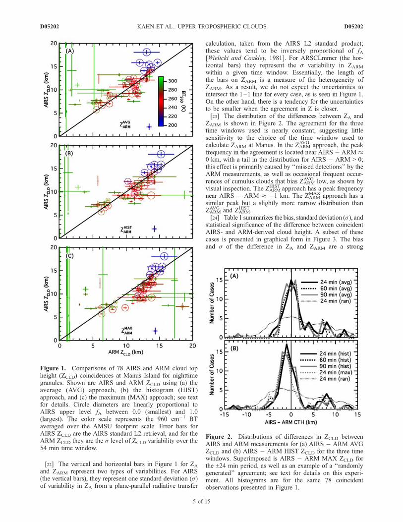
[22] The vertical and horizontal bars in Figure 1 for ZA

and ZARM represent two types of variabilities. For AIRS(the vertical bars), they represent one standard deviation (s)of variability in ZA from a plane-parallel radiative transfer

calculation, taken from the AIRS L2 standard product;these values tend to be inversely proportional of fA[Wielicki and Coakley, 1981]. For ARSCLmmcr (the hor-izontal bars) they represent the s variability in ZARM

within a given time window. Essentially, the length ofthe bars on ZARM is a measure of the heterogeneity ofZARM. As a result, we do not expect the uncertainties tointersect the 1–1 line for every case, as is seen in Figure 1.On the other hand, there is a tendency for the uncertaintiesto be smaller when the agreement in Z is closer.[23] The distribution of the differences between ZA and

ZARM is shown in Figure 2. The agreement for the threetime windows used is nearly constant, suggesting littlesensitivity to the choice of the time window used tocalculate ZARM at Manus. In the ZARM

AVG approach, the peakfrequency in the agreement is located near AIRS � ARM �0 km, with a tail in the distribution for AIRS � ARM > 0;this effect is primarily caused by ‘‘missed detections’’ by theARM measurements, as well as occasional frequent occur-rences of cumulus clouds that bias ZARM

AVG low, as shown byvisual inspection. The ZARM

HIST approach has a peak frequencynear AIRS � ARM � �1 km. The ZARM

MAX approach has asimilar peak but a slightly more narrow distribution thanZARMAVG and ZARM

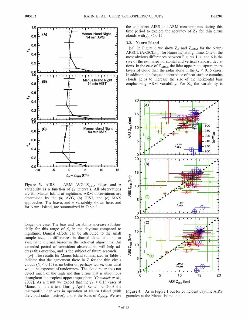
HIST.[24] Table 1 summarizes the bias, standard deviation (s), and

statistical significance of the difference between coincidentAIRS- and ARM-derived cloud height. A subset of thesecases is presented in graphical form in Figure 3. The biasand s of the difference in ZA and ZARM are a strong

Figure 1. Comparisons of 78 AIRS and ARM cloud topheight (ZCLD) coincidences at Manus Island for nighttimegranules. Shown are AIRS and ARM ZCLD using (a) theaverage (AVG) approach, (b) the histogram (HIST)approach, and (c) the maximum (MAX) approach; see textfor details. Circle diameters are linearly proportional toAIRS upper level fA between 0.0 (smallest) and 1.0(largest). The color scale represents the 960 cm�1 BTaveraged over the AMSU footprint scale. Error bars forAIRS ZCLD are the AIRS standard L2 retrieval, and for theARM ZCLD they are the s level of ZCLD variability over the54 min time window.

Figure 2. Distributions of differences in ZCLD betweenAIRS and ARM measurements for (a) AIRS � ARM AVGZCLD and (b) AIRS � ARM HIST ZCLD for the three timewindows. Superimposed is AIRS � ARM MAX ZCLD forthe ±24 min period, as well as an example of a ‘‘randomlygenerated’’ agreement; see text for details on this experi-ment. All histograms are for the same 78 coincidentobservations presented in Figure 1.

D05202 KAHN ET AL.: UPPER TROPOSPHERIC CLOUDS

5 of 15

D05202

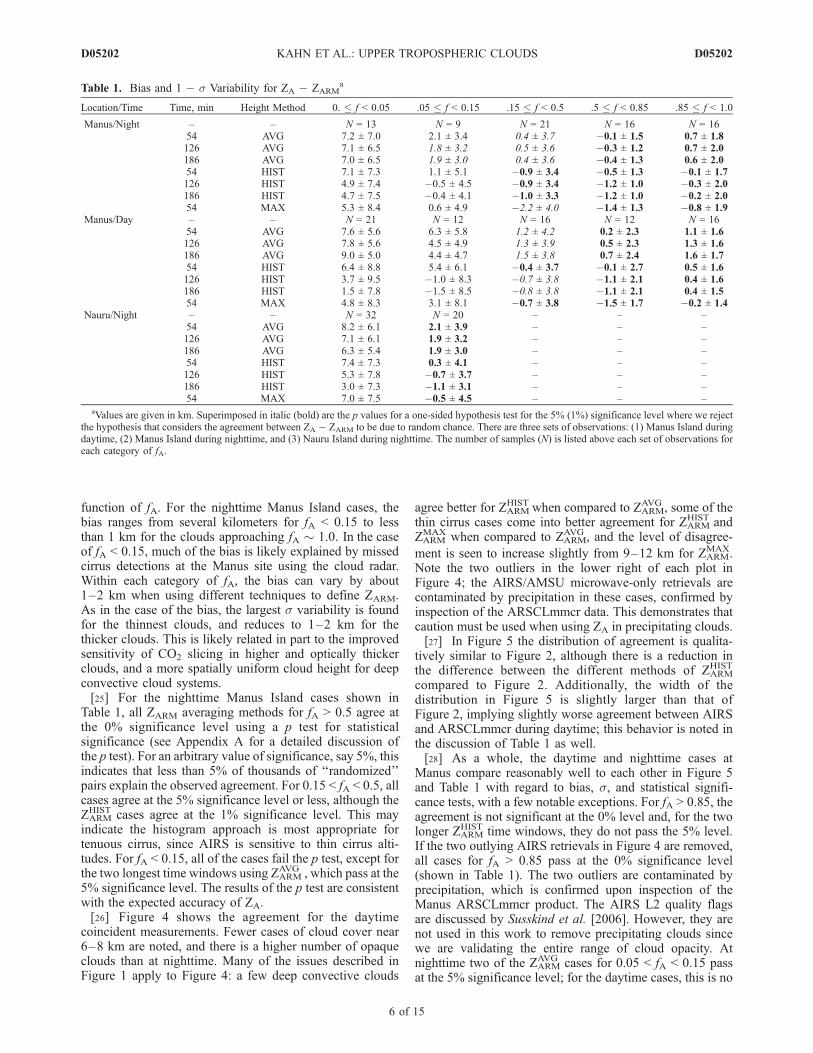
function of fA. For the nighttime Manus Island cases, thebias ranges from several kilometers for fA < 0.15 to lessthan 1 km for the clouds approaching fA � 1.0. In the caseof fA < 0.15, much of the bias is likely explained by missedcirrus detections at the Manus site using the cloud radar.Within each category of fA, the bias can vary by about1–2 km when using different techniques to define ZARM.As in the case of the bias, the largest s variability is foundfor the thinnest clouds, and reduces to 1–2 km for thethicker clouds. This is likely related in part to the improvedsensitivity of CO2 slicing in higher and optically thickerclouds, and a more spatially uniform cloud height for deepconvective cloud systems.[25] For the nighttime Manus Island cases shown in

Table 1, all ZARM averaging methods for fA > 0.5 agree atthe 0% significance level using a p test for statisticalsignificance (see Appendix A for a detailed discussion ofthe p test). For an arbitrary value of significance, say 5%, thisindicates that less than 5% of thousands of ‘‘randomized’’pairs explain the observed agreement. For 0.15 < fA < 0.5, allcases agree at the 5% significance level or less, although theZARMHIST cases agree at the 1% significance level. This may

indicate the histogram approach is most appropriate fortenuous cirrus, since AIRS is sensitive to thin cirrus alti-tudes. For fA < 0.15, all of the cases fail the p test, except forthe two longest time windows using ZARM

AVG , which pass at the5% significance level. The results of the p test are consistentwith the expected accuracy of ZA.[26] Figure 4 shows the agreement for the daytime

coincident measurements. Fewer cases of cloud cover near6–8 km are noted, and there is a higher number of opaqueclouds than at nighttime. Many of the issues described inFigure 1 apply to Figure 4: a few deep convective clouds

agree better for ZARMHIST when compared to ZARM

AVG , some of thethin cirrus cases come into better agreement for ZARM

HIST andZARMMAX when compared to ZARM

AVG , and the level of disagree-

ment is seen to increase slightly from 9–12 km for ZARMMAX.

Note the two outliers in the lower right of each plot inFigure 4; the AIRS/AMSU microwave-only retrievals arecontaminated by precipitation in these cases, confirmed byinspection of the ARSCLmmcr data. This demonstrates thatcaution must be used when using ZA in precipitating clouds.[27] In Figure 5 the distribution of agreement is qualita-

tively similar to Figure 2, although there is a reduction inthe difference between the different methods of ZARM

HIST

compared to Figure 2. Additionally, the width of thedistribution in Figure 5 is slightly larger than that ofFigure 2, implying slightly worse agreement between AIRSand ARSCLmmcr during daytime; this behavior is noted inthe discussion of Table 1 as well.[28] As a whole, the daytime and nighttime cases at

Manus compare reasonably well to each other in Figure 5and Table 1 with regard to bias, s, and statistical signifi-cance tests, with a few notable exceptions. For fA > 0.85, theagreement is not significant at the 0% level and, for the twolonger ZARM

HIST time windows, they do not pass the 5% level.If the two outlying AIRS retrievals in Figure 4 are removed,all cases for fA > 0.85 pass at the 0% significance level(shown in Table 1). The two outliers are contaminated byprecipitation, which is confirmed upon inspection of theManus ARSCLmmcr product. The AIRS L2 quality flagsare discussed by Susskind et al. [2006]. However, they arenot used in this work to remove precipitating clouds sincewe are validating the entire range of cloud opacity. Atnighttime two of the ZARM

AVG cases for 0.05 < fA < 0.15 passat the 5% significance level; for the daytime cases, this is no

Table 1. Bias and 1 � s Variability for ZA � ZARMa

Location/Time Time, min Height Method 0. � f < 0.05 .05 � f < 0.15 .15 � f < 0.5 .5 � f < 0.85 .85 � f < 1.0

Manus/Night – – N = 13 N = 9 N = 21 N = 16 N = 1654 AVG 7.2 ± 7.0 2.1 ± 3.4 0.4 ± 3.7 �0.1 ± 1.5 0.7 ± 1.8126 AVG 7.1 ± 6.5 1.8 ± 3.2 0.5 ± 3.6 �0.3 ± 1.2 0.7 ± 2.0186 AVG 7.0 ± 6.5 1.9 ± 3.0 0.4 ± 3.6 �0.4 ± 1.3 0.6 ± 2.054 HIST 7.1 ± 7.3 1.1 ± 5.1 �0.9 ± 3.4 �0.5 ± 1.3 �0.1 ± 1.7126 HIST 4.9 ± 7.4 �0.5 ± 4.5 �0.9 ± 3.4 �1.2 ± 1.0 �0.3 ± 2.0186 HIST 4.7 ± 7.5 �0.4 ± 4.1 �1.0 ± 3.3 �1.2 ± 1.0 �0.2 ± 2.054 MAX 5.3 ± 8.4 0.6 ± 4.9 �2.2 ± 4.0 �1.4 ± 1.3 �0.8 ± 1.9

Manus/Day – – N = 21 N = 12 N = 16 N = 12 N = 1654 AVG 7.6 ± 5.6 6.3 ± 5.8 1.2 ± 4.2 0.2 ± 2.3 1.1 ± 1.6126 AVG 7.8 ± 5.6 4.5 ± 4.9 1.3 ± 3.9 0.5 ± 2.3 1.3 ± 1.6186 AVG 9.0 ± 5.0 4.4 ± 4.7 1.5 ± 3.8 0.7 ± 2.4 1.6 ± 1.754 HIST 6.4 ± 8.8 5.4 ± 6.1 �0.4 ± 3.7 �0.1 ± 2.7 0.5 ± 1.6126 HIST 3.7 ± 9.5 �1.0 ± 8.3 �0.7 ± 3.8 �1.1 ± 2.1 0.4 ± 1.6186 HIST 1.5 ± 7.8 �1.5 ± 8.5 �0.8 ± 3.8 �1.1 ± 2.1 0.4 ± 1.554 MAX 4.8 ± 8.3 3.1 ± 8.1 �0.7 ± 3.8 �1.5 ± 1.7 �0.2 ± 1.4

Nauru/Night – – N = 32 N = 20 – – –54 AVG 8.2 ± 6.1 2.1 ± 3.9 – – –126 AVG 7.1 ± 6.1 1.9 ± 3.2 – – –186 AVG 6.3 ± 5.4 1.9 ± 3.0 – – –54 HIST 7.4 ± 7.3 0.3 ± 4.1 – – –126 HIST 5.3 ± 7.8 �0.7 ± 3.7 – – –186 HIST 3.0 ± 7.3 �1.1 ± 3.1 – – –54 MAX 7.0 ± 7.5 �0.5 ± 4.5 – – –

aValues are given in km. Superimposed in italic (bold) are the p values for a one-sided hypothesis test for the 5% (1%) significance level where we rejectthe hypothesis that considers the agreement between ZA � ZARM to be due to random chance. There are three sets of observations: (1) Manus Island duringdaytime, (2) Manus Island during nighttime, and (3) Nauru Island during nighttime. The number of samples (N) is listed above each set of observations foreach category of fA.

D05202 KAHN ET AL.: UPPER TROPOSPHERIC CLOUDS

6 of 15

D05202

longer the case. The bias and variability increase substan-tially for this range of fA in the daytime compared tonighttime. Diurnal effects can be attributed to the smallsample size, to differences in diurnal cloud amount, orsystematic diurnal biases in the retrieval algorithms. Anextended period of coincident observations will help ad-dress this question, and is the subject of future research.[29] The results for Manus Island summarized in Table 1

indicate that the agreement there in Z for the thin cirrusclouds (fA < 0.15) is no better or, perhaps worse, than whatwould be expected of randomness. The cloud radar does notdetect much of the high and thin cirrus that is ubiquitousthroughout the tropical upper troposphere [Comstock et al.,2002]. As a result we expect that the fA < 0.15 cases atManus fail the p test. During April–September 2003 themicropulse lidar was in operation at Nauru Island (withthe cloud radar inactive), and is the basis of ZARM. We use

the coincident AIRS and ARM measurements during thistime period to explore the accuracy of ZA for thin cirrusclouds with fA � 0.15.

3.2. Nauru Island

[30] In Figure 6 we show ZA and ZARM for the NauruARSCL (ARSCLmpl for Nauru Is.) at nighttime. One of themost obvious differences between Figures 1, 4, and 6 is thesize of the estimated horizontal and vertical standard devia-tions. In the case of ZARM, the lidar appears to capture morelayers of cloud than the radar alone in the fA � 0.15 cases.In addition, the frequent occurrence of near-surface cumulusclouds helps to increase the size of the horizontal barsemphasizing ARM variability. For ZA the variability is

Figure 3. AIRS � ARM AVG ZCLD biases and svariability as a function of fA intervals. All observationsare for Manus Island at nighttime. ARM observations aredetermined by the (a) AVG, (b) HIST, and (c) MAXapproaches. The biases and s variability shown here, andfor Nauru Island, are summarized in Table 1.

Figure 4. As in Figure 1 but for coincident daytime AIRSgranules at the Manus Island site.

D05202 KAHN ET AL.: UPPER TROPOSPHERIC CLOUDS

7 of 15

D05202

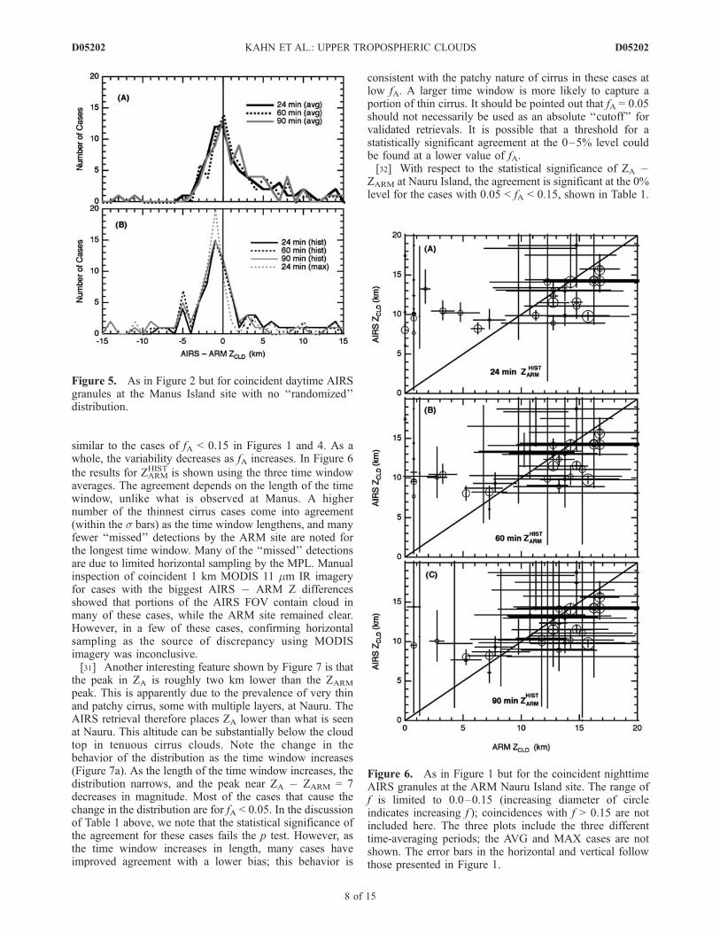
similar to the cases of fA < 0.15 in Figures 1 and 4. As awhole, the variability decreases as fA increases. In Figure 6

the results for ZARMHIST is shown using the three time window

averages. The agreement depends on the length of the timewindow, unlike what is observed at Manus. A highernumber of the thinnest cirrus cases come into agreement(within the s bars) as the time window lengthens, and manyfewer ‘‘missed’’ detections by the ARM site are noted forthe longest time window. Many of the ‘‘missed’’ detectionsare due to limited horizontal sampling by the MPL. Manualinspection of coincident 1 km MODIS 11 mm IR imageryfor cases with the biggest AIRS � ARM Z differencesshowed that portions of the AIRS FOV contain cloud inmany of these cases, while the ARM site remained clear.However, in a few of these cases, confirming horizontalsampling as the source of discrepancy using MODISimagery was inconclusive.[31] Another interesting feature shown by Figure 7 is that

the peak in ZA is roughly two km lower than the ZARM

peak. This is apparently due to the prevalence of very thinand patchy cirrus, some with multiple layers, at Nauru. TheAIRS retrieval therefore places ZA lower than what is seenat Nauru. This altitude can be substantially below the cloudtop in tenuous cirrus clouds. Note the change in thebehavior of the distribution as the time window increases(Figure 7a). As the length of the time window increases, thedistribution narrows, and the peak near ZA � ZARM = 7decreases in magnitude. Most of the cases that cause thechange in the distribution are for fA < 0.05. In the discussionof Table 1 above, we note that the statistical significance ofthe agreement for these cases fails the p test. However, asthe time window increases in length, many cases haveimproved agreement with a lower bias; this behavior is

consistent with the patchy nature of cirrus in these cases atlow fA. A larger time window is more likely to capture aportion of thin cirrus. It should be pointed out that fA = 0.05should not necessarily be used as an absolute ‘‘cutoff’’ forvalidated retrievals. It is possible that a threshold for astatistically significant agreement at the 0–5% level couldbe found at a lower value of fA.[32] With respect to the statistical significance of ZA �

ZARM at Nauru Island, the agreement is significant at the 0%level for the cases with 0.05 < fA < 0.15, shown in Table 1.

Figure 5. As in Figure 2 but for coincident daytime AIRSgranules at the Manus Island site with no ‘‘randomized’’distribution.

Figure 6. As in Figure 1 but for the coincident nighttimeAIRS granules at the ARM Nauru Island site. The range off is limited to 0.0–0.15 (increasing diameter of circleindicates increasing f ); coincidences with f > 0.15 are notincluded here. The three plots include the three differenttime-averaging periods; the AVG and MAX cases are notshown. The error bars in the horizontal and vertical followthose presented in Figure 1.

D05202 KAHN ET AL.: UPPER TROPOSPHERIC CLOUDS

8 of 15

D05202

This is a vast improvement over the statistical significanceat Manus Island for the same range of fA. The bias and svariability is approximately �1.1 to 2.1 km ± 3.0 to 4.5 km;this compares to �1.5 to 6.3 ± 3.0 to 8.5 km at Manus.Recall from Table 1 that the range of values results fromusing different approaches to determine ZARM and themagnitude of fA. We attribute the better agreement at Nauruto the differences in the sensitivity of the lidar to thin cirrusclouds, consistent with previously published results[Comstock et al., 2002]. The Nauru comparison highlightsthe sensitivity of the AIRS upper level cloud top pressureproduct to tenuous cirrus clouds. A statistically meaningfulsampling rate requires a larger set of cases in order to reducethe width of the fA bins and keep the number of cases ineach bin large enough so that a representative subsampleof observed cloud variability is obtained. CloudSat andCALIPSO will provide a much larger set of collocatedobservations, and they will mostly eliminate cloud evolu-tion as a means of disagreement because of their close timecoincidence to AIRS.

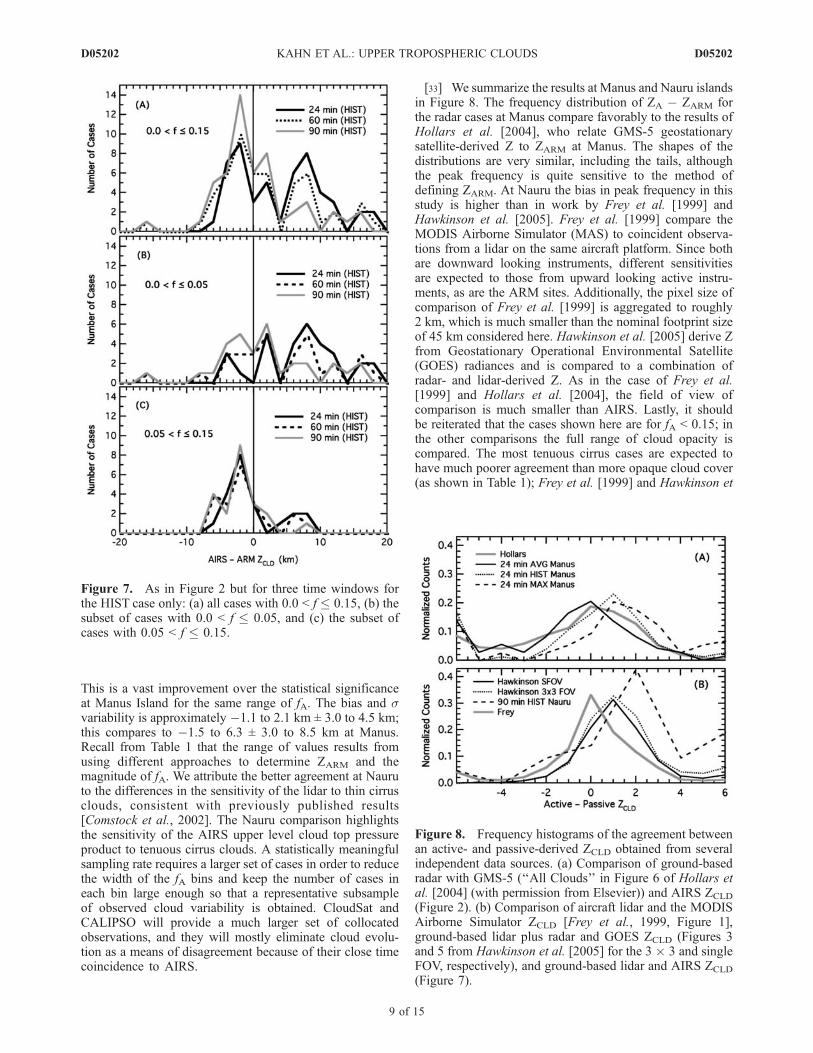
[33] We summarize the results at Manus and Nauru islandsin Figure 8. The frequency distribution of ZA � ZARM forthe radar cases at Manus compare favorably to the results ofHollars et al. [2004], who relate GMS-5 geostationarysatellite-derived Z to ZARM at Manus. The shapes of thedistributions are very similar, including the tails, althoughthe peak frequency is quite sensitive to the method ofdefining ZARM. At Nauru the bias in peak frequency in thisstudy is higher than in work by Frey et al. [1999] andHawkinson et al. [2005]. Frey et al. [1999] compare theMODIS Airborne Simulator (MAS) to coincident observa-tions from a lidar on the same aircraft platform. Since bothare downward looking instruments, different sensitivitiesare expected to those from upward looking active instru-ments, as are the ARM sites. Additionally, the pixel size ofcomparison of Frey et al. [1999] is aggregated to roughly2 km, which is much smaller than the nominal footprint sizeof 45 km considered here. Hawkinson et al. [2005] derive Zfrom Geostationary Operational Environmental Satellite(GOES) radiances and is compared to a combination ofradar- and lidar-derived Z. As in the case of Frey et al.[1999] and Hollars et al. [2004], the field of view ofcomparison is much smaller than AIRS. Lastly, it shouldbe reiterated that the cases shown here are for fA < 0.15; inthe other comparisons the full range of cloud opacity iscompared. The most tenuous cirrus cases are expected tohave much poorer agreement than more opaque cloud cover(as shown in Table 1); Frey et al. [1999] and Hawkinson et

Figure 7. As in Figure 2 but for three time windows forthe HIST case only: (a) all cases with 0.0 < f � 0.15, (b) thesubset of cases with 0.0 < f � 0.05, and (c) the subset ofcases with 0.05 < f � 0.15.

Figure 8. Frequency histograms of the agreement betweenan active- and passive-derived ZCLD obtained from severalindependent data sources. (a) Comparison of ground-basedradar with GMS-5 (‘‘All Clouds’’ in Figure 6 of Hollars etal. [2004] (with permission from Elsevier)) and AIRS ZCLD

(Figure 2). (b) Comparison of aircraft lidar and the MODISAirborne Simulator ZCLD [Frey et al., 1999, Figure 1],ground-based lidar plus radar and GOES ZCLD (Figures 3and 5 from Hawkinson et al. [2005] for the 3 � 3 and singleFOV, respectively), and ground-based lidar and AIRS ZCLD

(Figure 7).

D05202 KAHN ET AL.: UPPER TROPOSPHERIC CLOUDS

9 of 15

D05202

al. [2005] can be expected to have better agreement than theresults presented here for Nauru.

4. Comparing AIRS and MLS Cloud Properties

4.1. Different Perspectives of Coincident Cloud Fields

[34] The eight minute difference in measurements ofclouds by the AIRS and MLS instruments provide a uniqueopportunity to cross examine AIRS cloud height andfraction fields with a large number of near-simultaneouscoincident MLS IWC measurements. This offers the poten-tial of characterizing the 3-D spatial state of high-levelcloudiness [Liou et al., 2002]. Nadir IR sounding instru-ments, such as AIRS, have limitations in resolving verticalcloud structure but have good horizontal resolution. Con-versely, limb instruments like the MLS have limitations intheir horizontal field of view, but are ideal for makingmeasurements of clouds at fine vertical resolution. Thetwo very different cloud measurements can be comparedif the limitations and strengths of each measurement areunderstood in terms of the sensitivity to particular cloudsystems.[35] AIRS and MLS have numerous differences in their

instrumentation, measurement wavelengths, retrieval tech-niques, and viewing geometry. The MLS senses throughclouds horizontally in thin vertical layers, while AIRSobserves radiance from a vertical or near-vertical atmo-spheric column. Because the effective size, size distribution,and habit of ice particles significantly attenuate radiance asa function of wavelength, the AIRS and MLS instrumentseffectively observe different parts of the same cloud. Be-cause MLS views in the forward along-track direction, withthe tangent altitude trailing the AIRS nadir observations byapproximately 8 min, the instrument, wavelength, retrievaltechnique, and viewing geometry-related differences likelydominate over those due to cloud evolution. However, cloudevolution should not be dismissed, especially in rapidlyevolving convective systems. Vertical velocities greater than10 m s�1 are not uncommon in convective systems; thistranslates to a distance >4 km in an 8 min period.[36] MLS is sensitive in detecting ice particles from a few

tens to a few hundreds of microns in diameter in opticallydense clouds [Wu et al., 2006]. It is able to sense into andthrough many thick cumulonimbus clouds such as thoseassociated with deep convection and anvil outflow but canmiss thin cirrus composed of smaller ice particles. TheAIRS instrument is most sensitive to tenuous clouds butsaturates around an IR optical depth above 5 [Huang et al.,2004]. A tradeoff exists between the reduced sensitivity ofMLS to small particle ice clouds compared to AIRS, and thelonger limb-viewing path length of MLS (about an order ofmagnitude longer than the nadir view); see Liao et al.[1995] and Kahn et al. [2002, and references therein] forfurther discussion on the detection sensitivity due to view-ing geometry. Also, the MLS reports IWC at discretepressure levels, and AIRS reports cloud top pressure (PA)at a continuous range of altitudes.[37] We compare the MLS IWC to PA for each of the six

pressure levels between 82 and 215 hPa. The best MLSsensitivity to cloud top height is at 100–147 hPa. MLSlevels are discrete and PA is continuous, necessitating acomparison on an MLS level-by-level basis. The compar-

isons are subcategorized as a function of the AIRS upperlevel cloud fraction (fA) and MLS IWC. We define the MLScloud top pressure (PM) as the highest altitude (lowestpressure) with IWC > 0 mg/m3. Some values of cloud-induced radiance are below a nominal clear-sky uncertainty;the sensitivity of the agreement to removing such cases willbe discussed.[38] The AIRS PA horizontal FOV is roughly circular at

�45 km, and the MLS FOV is 165 km� 7 km (along track�cross track), complicating comparisons in heterogeneouscloud cover. Thus we represent PA in two ways: the threenearest PA retrievals to the MLS 100 hPa tangent point alongthe line of sight are averaged (PAVG), and the lowest value ofPA (highest altitude) among the three nearest PA retrievals isdefined as PHI. In the case of PAVG the total horizontal AIRSFOV along the MLS line of sight is roughly 135 � 45 km(along track� cross track), which is considerably wider thanMLS cross-track FOV. In the case of PHI previous studies ofclouds in occultation measurements [Kahn et al., 2002, andreferences therein] suggest the cloud may fill a very smallportion of the FOValong the line of sight; this motivates theuse of PHI for determining PA.

4.2. Results

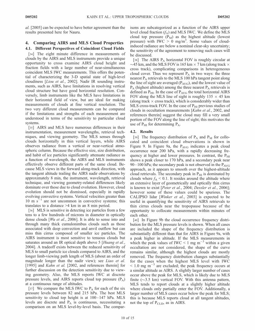
[39] The frequency distribution of PA and PM for collo-cated and coincident cloud observations is shown inFigure 9. In Figure 9a, the PAVG indicates a peak cloudoccurrence near 200 hPa, with a rapidly decreasing fre-quency at higher and lower pressures. In contrast, the PHIshows a peak closer to 170 hPa, and a secondary peak near90–100 hPa; the secondary peak is not observed in the PAVGapproach, as it appears to smooth over the highest-altitudecloud retrievals. The secondary peak in PHI is dominated byclouds where fA < 0.1. It resides around the altitude wherean extensive layer of geometrically and optically thin cirrusis known to exist [Peter et al., 2004; Dessler et al., 2006];however some of these values could be spurious. TheCALIPSO lidar [Winker et al., 2003] is expected to beuseful in quantifying the sensitivity of AIRS retrievals tothin cirrus clouds near the tropopause because of theopportunity to collocate measurements within minutes ofeach other.[40] In Figure 9b the cloud occurrence frequency distri-

bution for the MLS pressure levels is shown. When all casesare included the shape of the frequency distribution issubstantially different than that for AIRS in Figure 9a, witha peak higher in altitude. If the MLS measurements inwhich the peak values of IWC < 1 mg m�3 within a givenoccultation are not considered, the shape of the curveremains similar, although the highest clouds are mostlyremoved. The frequency distribution changes substantiallyfor the cases when the highest MLS level with IWC< 1.0 mg m�3 are excluded; the peak frequency occurs ata similar altitude as AIRS. A slightly larger number of casesoccur above the peak for MLS, which is likely due to MLSfinite (�3.5 km) vertical FOV. With this antenna pattern,MLS tends to report clouds at a slightly higher altitudewhere clouds only partially enter the FOV. Additionally, alarger number of MLS cases occur below the peak for MLS;this is because MLS reports cloud at all tangent altitudes,not the top of PCLD, as in AIRS.

D05202 KAHN ET AL.: UPPER TROPOSPHERIC CLOUDS

10 of 15

D05202

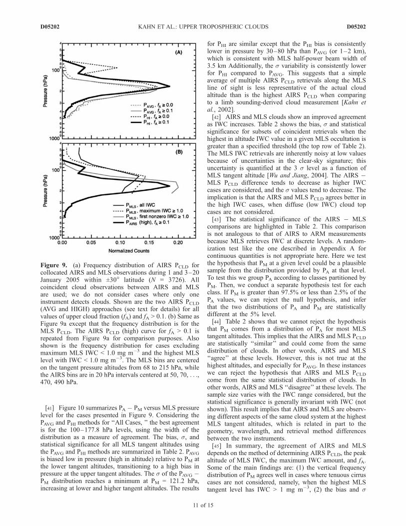
[41] Figure 10 summarizes PA � PM versus MLS pressurelevel for the cases presented in Figure 9. Considering thePAVG and PHI methods for ‘‘All Cases, ’’ the best agreementis for the 100–177.8 hPa levels, using the width of thedistribution as a measure of agreement. The bias, s, andstatistical significance for all MLS tangent altitudes usingthe PAVG and PHI methods are summarized in Table 2. PAVGis biased low in pressure (high in altitude) relative to PM atthe lower tangent altitudes, transitioning to a high bias inpressure at the upper tangent altitudes. The s of the PAVG �PM distribution reaches a minimum at PM = 121.2 hPa,increasing at lower and higher tangent altitudes. The results

for PHI are similar except that the PHI bias is consistentlylower in pressure by 30–80 hPa than PAVG (or 1–2 km),which is consistent with MLS half-power beam width of3.5 km Additionally, the s variability is consistently lowerfor PHI compared to PAVG. This suggests that a simpleaverage of multiple AIRS PCLD retrievals along the MLSline of sight is less representative of the actual cloudaltitude than is the highest AIRS PCLD when comparingto a limb sounding-derived cloud measurement [Kahn etal., 2002].[42] AIRS and MLS clouds show an improved agreement

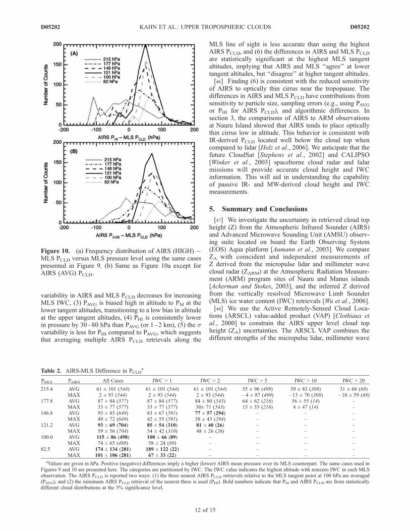
as IWC increases. Table 2 shows the bias, s and statisticalsignificance for subsets of coincident retrievals when thehighest in altitude IWC value in a given MLS occultation isgreater than a specified threshold (the top row of Table 2).The MLS IWC retrievals are inherently noisy at low valuesbecause of uncertainties in the clear-sky signature; thisuncertainty is quantified at the 3 s level as a function ofMLS tangent altitude [Wu and Jiang, 2004]. The AIRS �MLS PCLD difference tends to decrease as higher IWCcases are considered, and the s values tend to decrease. Theimplication is that the AIRS and MLS PCLD agrees better inthe high IWC cases, when diffuse (low IWC) cloud topcases are not considered.[43] The statistical significance of the AIRS � MLS

comparisons are highlighted in Table 2. This comparisonis not analogous to that of AIRS to ARM measurementsbecause MLS retrieves IWC at discrete levels. A random-ization test like the one described in Appendix A forcontinuous quantities is not appropriate here. Here we testthe hypothesis that PM at a given level could be a plausiblesample from the distribution provided by PA at that level.To test this we group PA according to classes partitioned byPM. Then, we conduct a separate hypothesis test for eachclass. If PM is greater than 97.5% or less than 2.5% of thePA values, we can reject the null hypothesis, and inferthat the two distributions of PA and PM are statisticallydifferent at the 5% level.[44] Table 2 shows that we cannot reject the hypothesis

that PM comes from a distribution of PA for most MLStangent altitudes. This implies that the AIRS and MLS PCLDare statistically ‘‘similar’’ and could come from the samedistribution of clouds. In other words, AIRS and MLS‘‘agree’’ at these levels. However, this is not true at thehighest altitudes, and especially for PAVG. In these instanceswe can reject the hypothesis that AIRS and MLS PCLDcome from the same statistical distribution of clouds. Inother words, AIRS and MLS ‘‘disagree’’ at these levels. Thesample size varies with the IWC range considered, but thestatistical significance is generally invariant with IWC (notshown). This result implies that AIRS and MLS are observ-ing different aspects of the same cloud system at the highestMLS tangent altitudes, which is related in part to thegeometry, wavelength, and retrieval method differencesbetween the two instruments.[45] In summary, the agreement of AIRS and MLS

depends on the method of determining AIRS PCLD, the peakaltitude of MLS IWC, the maximum IWC amount, and fA.Some of the main findings are: (1) the vertical frequencydistribution of PM agrees well in cases where tenuous cirruscases are not considered, namely, when the highest MLStangent level has IWC > 1 mg m�3, (2) the bias and s

Figure 9. (a) Frequency distribution of AIRS PCLD forcollocated AIRS and MLS observations during 1 and 3–20January 2005 within ±30� latitude (N = 3726). Allcoincident cloud observations between AIRS and MLSare used; we do not consider cases where only oneinstrument detects clouds. Shown are the two AIRS PCLD(AVG and HIGH) approaches (see text for details) for allvalues of upper cloud fraction (fA) and fA > 0.1. (b) Same asFigure 9a except that the frequency distribution is for theMLS PCLD. The AIRS PCLD (high) curve for fA > 0.1 isrepeated from Figure 9a for comparison purposes. Alsoshown is the frequency distribution for cases excludingmaximum MLS IWC < 1.0 mg m�3 and the highest MLSlevel with IWC < 1.0 mg m�3. The MLS bins are centeredon the tangent pressure altitudes from 68 to 215 hPa, whilethe AIRS bins are in 20 hPa intervals centered at 50, 70, . . .,470, 490 hPa.

D05202 KAHN ET AL.: UPPER TROPOSPHERIC CLOUDS

11 of 15

D05202

variability in AIRS and MLS PCLD decreases for increasingMLS IWC, (3) PAVG is biased high in altitude to PM at thelower tangent altitudes, transitioning to a low bias in altitudeat the upper tangent altitudes, (4) PHI is consistently lowerin pressure by 30–80 hPa than PAVG (or 1–2 km), (5) the svariability is less for PHI compared to PAVG, which suggeststhat averaging multiple AIRS PCLD retrievals along the

MLS line of sight is less accurate than using the highestAIRS PCLD, and (6) the differences in AIRS and MLS PCLDare statistically significant at the highest MLS tangentaltitudes, implying that AIRS and MLS ‘‘agree’’ at lowertangent altitudes, but ‘‘disagree’’ at higher tangent altitudes.[46] Finding (6) is consistent with the reduced sensitivity

of AIRS to optically thin cirrus near the tropopause. Thedifferences in AIRS and MLS PCLD have contributions fromsensitivity to particle size, sampling errors (e.g., using PAVGor PHI for AIRS PCLD), and algorithmic differences. Insection 3, the comparisons of AIRS to ARM observationsat Nauru Island showed that AIRS tends to place opticallythin cirrus low in altitude. This behavior is consistent withIR-derived PCLD located well below the cloud top whencompared to lidar [Holz et al., 2006]. We anticipate that thefuture CloudSat [Stephens et al., 2002] and CALIPSO[Winker et al., 2003] spaceborne cloud radar and lidarmissions will provide accurate cloud height and IWCinformation. This will aid in understanding the capabilityof passive IR- and MW-derived cloud height and IWCmeasurements.

5. Summary and Conclusions

[47] We investigate the uncertainty in retrieved cloud topheight (Z) from the Atmospheric Infrared Sounder (AIRS)and Advanced Microwave Sounding Unit (AMSU) observ-ing suite located on board the Earth Observing System(EOS) Aqua platform [Aumann et al., 2003]. We compareZA with coincident and independent measurements ofZ derived from the micropulse lidar and millimeter wavecloud radar (ZARM) at the Atmospheric Radiation Measure-ment (ARM) program sites of Nauru and Manus islands[Ackerman and Stokes, 2003], and the inferred Z derivedfrom the vertically resolved Microwave Limb Sounder(MLS) ice water content (IWC) retrievals [Wu et al., 2006].[48] We use the Active Remotely-Sensed Cloud Loca-

tions (ARSCL) value-added product (VAP) [Clothiaux etal., 2000] to constrain the AIRS upper level cloud topheight (ZA) uncertainties. The ARSCL VAP combines thedifferent strengths of the micropulse lidar, millimeter wave

Table 2. AIRS-MLS Difference in PCLDa

PMLS PAIRS All Cases IWC > 1 IWC > 2 IWC > 5 IWC > 10 IWC > 20

215.4 AVG 61 ± 101 (544) 61 ± 101 (544) 61 ± 101 (544) 55 ± 96 (499) 39 ± 83 (308) 31 ± 68 (68)MAX 2 ± 93 (544) 2 ± 93 (544) 2 ± 93 (544) �4 ± 87 (499) �13 ± 70 (308) �10 ± 59 (68)

177.8 AVG 87 ± 84 (577) 87 ± 84 (577) 84 ± 80 (543) 64 ± 62 (216) 56 ± 55 (14) –MAX 33 ± 77 (577) 33 ± 77 (577) 30± 71 (543) 15 ± 55 (216) 4 ± 47 (14) –

146.8 AVG 93 ± 85 (649) 83 ± 67 (591) 77 ± 57 (294) – – –MAX 49 ± 72 (649) 42 ± 55 (591) 38 ± 43 (294) – – –

121.2 AVG 93 ± 69 (704) 85 ± 54 (310) 81 ± 40 (26) – – –MAX 59 ± 56 (704) 54 ± 42 (310) 48 ± 26 (26) – – –

100.0 AVG 115 ± 86 (498) 100 ± 66 (89) – – – –MAX 74 ± 65 (498) 58 ± 24 (89) – – – –

82.5 AVG 174 ± 134 (281) 189 ± 122 (22) – – – –MAX 101 ± 106 (281) 67 ± 33 (22) – – – –

aValues are given in hPa. Positive (negative) differences imply a higher (lower) AIRS mean pressure over its MLS counterpart. The same cases used inFigures 9 and 10 are presented here. The categories are partitioned by IWC. The IWC value indicates the highest altitude with nonzero IWC in each MLSobservation. The AIRS PCLD is reported two ways: (1) the three nearest AIRS PCLD retrievals relative to the MLS tangent point at 100 hPa are averaged(PAVG), and (2) the minimum AIRS PCLD retrieval of the nearest three is used (PHI). Bold numbers indicate that PM and AIRS PCLD are from statisticallydifferent cloud distributions at the 5% significance level.

Figure 10. (a) Frequency distribution of AIRS (HIGH) �MLS PCLD versus MLS pressure level using the same casespresented in Figure 9. (b) Same as Figure 10a except forAIRS (AVG) PCLD.

D05202 KAHN ET AL.: UPPER TROPOSPHERIC CLOUDS

12 of 15

D05202

cloud radar, microwave radiometer, and laser ceilometerinto a single cloud top and base product, allowing for acomprehensive database for clouds with varying heights andthicknesses, optical depths (t), and hydrometeor character-istics. For a limited set of AIRS overpasses coincident withManus and Nauru islands (April–September 2003), onlythe cloud radar was in operation at Manus, and only themicropulse lidar was operational at Nauru. The primaryfindings of the AIRS � ARM comparisons are as follows.[49] 1. AIRS is sensitive to a wide range of clouds, with

statistically significant agreement of AIRS and ARM ZCLD

for an effective cloud fraction (fA) > 0.05.[50] 2. For all cases of fA > 0.15 at Manus using the cloud

radar only, the mean difference and s variability inZA � ZARM ranges from �2.2 to 1.6 km ± 1.0 to 4.2 km.The range of values is a result of using different techniquesto determine ZARM, as well as day/night differences.[51] 3. The differences between ZA and ZARM are not a

function of the length of the time window at Manus usingthe cloud radar, but time window dependence is seen atNauru for tenuous cirrus using the micropulse lidar, sug-gesting that ARM sampling biases are a function of cloudopacity and the ARM instrument being used.[52] 4. The three height methods give consistently

different results in ZA � ZARM; these differences are larger(smaller) for smaller (larger) fA. Cloud heights determinedfrom Cloudsat and CALIPSO will help determine thecloud types for which these averaging methods are mostappropriate.[53] 5. For the cases of 0.05 � fA < 0.15 at Nauru using

the micropulse lidar only, the mean difference and svariability in the agreement is �1.1 to 2.1 km ± 3.0 to4.5 km. This agreement is substantially improved over thatusing the cloud radar at Manus for this range of fA, anddemonstrates the sensitivity of AIRS to thin cirrus.[54] The near simultaneous measurements of clouds by

the AIRS and MLS instruments permit cross examination ofhorizontally resolved cloud height and fraction fields withvertically resolved ice water content (IWC). Comparisons ofcloud top pressure (PCLD) inferred from coincident AIRSand MLS IWC retrievals show that the mean differencedepends upon the method for determining AIRS PCLD (aswith the ARM comparisons), the peak altitude and maxi-mum value of MLS IWC, and fA. The primary findings ofthe AIRS � MLS comparisons are as follows.[55] 1. The bias and s variability of AIRS � MLS PCLD

decreases for increasing MLS IWC. The best agreement isseen when comparisons are limited to fA > 0.1 and IWC >1.0 mg m�3.[56] 2. When using the highest AIRS PCLD (abbreviated

as PHI) along the MLS tangent line of sight, the bias is lowerin pressure by 30–80 hPa than when averaging the nearestthree AIRS retrievals of PCLD (abbreviated as PAVG).[57] 3. The s variability is consistently lower for PHI

compared to PAVG, suggesting that an average of multipleAIRS PCLD retrievals along the MLS line of sight is oftenless accurate than using the highest AIRS PCLD.[58] 4. Differences in AIRS and MLS PCLD are statisti-

cally significant at the highest MLS tangent altitudes. Thisimplies that AIRS and MLS statistically ‘‘agree’’ at lowertangent altitudes, but ‘‘disagree’’ at higher tangent altitudes.

The disagreement occurs in regions dominated by tenuouscirrus near the tropopause.[59] Both AIRS and MLS have strengths and weaknesses

in their abilities to sense cloud structure. The AIRS iscapable of providing wide swaths of vertically integratedIR radiances, while the MLS is ideal for making measure-ments of clouds at discrete vertical intervals because of thelimb viewing geometry. This paper offers initial insightsinto upper tropospheric cloud structure as observed byAIRS and MLS using surface-based ARM measurements.By cross comparing the retrieved cloud quantities of instru-ments like AIRS and MLS (which view the same cloudfields from very different viewing perspectives) to activecloud radar and lidar observations of clouds, a step towardcharacterizing the 3-D picture of upper tropospheric cloudstructure is taken.

Appendix A

[60] This is a description of the test of the null hypothesisthat observed agreement is due to randomness alone.Specifically, for each case in Table 1 (the different defini-tions of ZARM categorized by fA), we begin with a set ofbivariate data points (ZARM, ZA), i = 1, . . ., N, where N isthe number of data point pairs. We measure the agreementbetween ZARM and ZA by D, defined below as

D ¼ 1

N

XN

i¼1

ZA � ZARMð Þ2: ðA1Þ

The value D is the average of the squared differencesbetween ZA and ZARM on the L2 norm, since the dynamicrange of the variables is small [Menke, 1989]. We calculatethe true value of delta (D*), as shown in equation (A1),using N data point pairs. Then, we simulate the distributionof D under the assumption that ZA and ZARM are notrelated. For each of B = 10,000 trials in our simulation, werandomly reordered the ZARM values and computed Db, forb = 1, . . ., B. The histogram of Db is an estimate of theso-called ‘‘null distribution’’ ofD: the distribution under theassumption that the null hypothesis is true. The p valueof the hypothesis test is the proportion of Db less than orequal to D*. Typically, the null hypothesis is rejected if thep value is less than 0.05 or, with a stricter standard, 0.01,corresponding to 5% and 1% confidence.[61] Resampling tests rely on assumptions that the data are

a representative sample of the population from which theyare drawn; in this case, the hypothetical population ofD* wewould obtain were we able to examine all possible coinci-dent ZA and ZARM. Since the sample sizes (N) here arerelatively small (N < 20 in most cases), the validity of theseresults is heavily dependent on the assumption of represen-tativeness. There are (at least) three reasons to believe thatthe sample is reasonably representative: (1) each coincidentcase has been inspected individually and is seen to representa wide variety of cloud scenes within each category of fA,(2) the conclusions drawn from these results are consistentwith the expected sensitivity of ZA and ZARM, and (3) thehistograms of the comparison compare favorably with thosefrom other data sources. A longer time series of collocated

D05202 KAHN ET AL.: UPPER TROPOSPHERIC CLOUDS

13 of 15

D05202

measurements will likely give an increased level of repre-sentativeness.

[62] Acknowledgments. The authors thank John Blaisdell for detaileddiscussion on the AIRS cloud retrieval system. We thank all colleagues onthe AIRS and MLS teams for support and helpful comments and twoanonymous reviewers for improvements to the manuscript. B. H. K. wasfunded by a National Research Council Resident Research Associatefellowship while in residence at NASA’s Jet Propulsion Laboratory (JPL).Value-added product data were obtained from the Atmospheric RadiationMeasurement (ARM) Program sponsored by the U.S. Department of Energy,Office of Science, Office of Biological and Environmental Research,Climate Change Research Division. This work was performed at JPL,California Institute of Technology, Pasadena, California, under contract withNASA.

ReferencesAckerman, T. P., and G. M. Stokes (2003), The Atmospheric RadiationMeasurement program, Phys. Today, 56, 38–44.

Aumann, H. H., et al. (2003), AIRS/AMSU/HSB on the Aqua mission:Design, science objectives, data products, and processing systems, IEEETrans. Geosci. Remote Sens., 41, 253–264.

Baum, B. A., and B. A. Wielicki (1994), Cirrus cloud retrievals usinginfrared sounding data: Multilevel cloud errors, J. Appl. Meteorol., 33,107–117.

Berendes, T. A., D. A. Berendes, R. M. Welch, E. G. Dutton, T. Uttal, andE. E. Clothiaux (2004), Cloud cover comparisons of the MODIS daytimecloud mask with surface instruments at the north slope of Alaska ARMsite, IEEE Trans. Geosci. Remote Sens., 42, 2584–2593.

Cahalan, R. F., and J. H. Joseph (1989), Fractal statistics of cloud fields,Mon. Weather Rev., 117, 261–272.

Chahine, M. T. (1974), Remote sounding of cloudy atmospheres. I. Thesingle cloud layer, J. Atmos. Sci., 31, 233–243.

Chylek, P., and C. Borel (2004), Mixed phase cloud water/ice structurefrom high spatial resolution satellite data, Geophys. Res. Lett., 31,L14104, doi:10.1029/2004GL020428.

Clothiaux, E. E., T. P. Ackerman, G. G. Mace, K. P. Moran, R. T. Marchand,M. A. Miller, and B. E. Martner (2000), Objective determination of cloudheights and radar reflectivities using a combination of active remote sen-sors at the ARM CART sites, J. Appl. Meteorol., 39, 645–665.

Comstock, J. M., and C. Jakob (2004), Evaluation of tropical cirrus cloudproperties derived from ECMWF model output and ground based mea-surements over Nauru Island, Geophys. Res. Lett., 31, L10106,doi:10.1029/2004GL019539.

Comstock, J. M., T. P. Ackerman, and G. G. Mace (2002), Ground-basedlidar and radar remote sensing of tropical cirrus clouds at Nauru Island:Cloud statistics and radiative impacts, J. Geophys. Res., 107(D23), 4714,doi:10.1029/2002JD002203.

Cooper, S. J., T. S. L’Ecuyer, and G. L. Stephens (2003), The impact ofexplicit cloud boundary information on ice cloud microphysical propertyretrievals from infrared radiances, J. Geophys. Res., 108(D3), 4107,doi:10.1029/2002JD002611.

Cracknell, A. P. (1998), Synergy in remote sensing–what’s in a pixel?, Int.J. Remote Sens., 19, 2025–2047.

Cunningham, J. D., and J. M. Haas (2004), NPOESS instruments: The futureof METSAT observations, paper presented at 11th Conference on SatelliteMeteorology and Oceanography, Am. Meteorol. Soc., Seattle, Wash.

Dessler, A. E., S. P. Palm,W. D. Hart, and J. D. Spinhirne (2006), Tropopause-level thin cirrus coverage revealed by ICESat/Geoscience Laser AltimeterSystem, J. Geophys. Res., 111, D08203, doi:10.1029/2005JD006586.

Elouragini, S., H. Chtioui, and P. H. Flamant (2005), Lidar remote soundingof cirrus clouds and comparison of simulated fluxes with surface andMETEOSAT observations, Atmos. Res., 73, 23–36.

Fetzer, E. J., B. H. Lambrigtsen, A. Eldering, H. H. Aumann, and M. T.Chahine (2006), Biases in total precipitable water vapor climatologiesfrom Atmospheric Infrared Sounder and Advanced Microwave ScanningRadiometer, J. Geophys. Res., 111, D09S16, doi:10.1029/2005JD006598.

Frey, R. A., B. A. Baum, W. P. Menzel, S. A. Ackerman, C. C. Moeller, andJ. D. Spinhirne (1999), A comparison of cloud top heights computedfrom airborne lidar and MAS radiance data using CO2 slicing, J. Geophys.Res., 104, 24,547–24,555.

Garrett, T. J., H. Gerber, D. G. Baumgardner, C. H. Twohy, and E. M.Weinstock (2003), Small, highly reflective ice crystals in low-latitudecirrus, Geophys. Res. Lett., 30(21), 2132, doi:10.1029/2003GL018153.

Gettelman, A., W. D. Collins, E. J. Fetzer, A. Eldering, F. W. Irion, P. B.Duffy, and G. Bala (2006), Climatology of upper tropospheric relativehumidity from the Atmospheric Infrared Sounder and implications forclimate, J. Clim., 19, 6104–6121.

Hawkinson, J. A., W. Feltz, and S. A. Ackerman (2005), A comparison ofGOES sounder– and cloud lidar– and radar– retrieved cloud-top heights,J. Appl. Meteorol., 44, 1234–1242.

Heymsfield, A. J., and G. M. McFarquhar (2002), Mid-latitude and tropicalcirrus: Microphysical properties, in Cirrus, edited by D. K. Lynch et al.,pp. 433–448, Oxford Univ. Press, New York.

Hollars, S., Q. Fu, J. Comstock, and T. Ackerman (2004), Comparison ofcloud-top height retrievals from ground-based 35 GHz MMCR andGMS-5 satellite observations at ARM TWP Manus site, Atmos. Res.,72, 169–186.

Holz, R. E., S. Ackerman, P. Antonelli, F. Nagle, R. O. Knuteson, M. McGill,D. L. Hlavka, and W. D. Hart (2006), An improvement to the high spectralresolutionCO2 slicing cloud top altitude retrieval, J. Atmos. Oceanic Technol.,23, 653–670.

Horvath, A., and R. Davies (2004), Anisotropy of water cloud reflectance:A comparison of measurements and 1D theory, Geophys. Res. Lett., 31,L01102, doi:10.1029/2003GL018386.

Huang, H.-L., P. Yang, H. Wei, B. A. Baum, Y. Hu, P. Antonelli, and S. A.Ackerman (2004), Inference of ice cloud properties from high spectralresolution infrared observations, IEEE Trans Geosci. Remote Sens., 42,842–853.

Intergovernmental Panel on Climate Change (2001), Climate Change 2001:The Scientific Basis, edited by J. T. Houghton et al., 881 pp., CambridgeUniv. Press, New York.

Kahn, B. H., A. Eldering, F. W. Irion, F. P. Mills, B. Sen, and M. R. Gunson(2002), Cloud identification in Atmospheric Trace Molecule Spectro-scopy infrared occultation measurements, Appl. Opt., 41, 2768–2780.

Kahn, B. H., K. N. Liou, S.-Y. Lee, E. F. Fishbein, S. DeSouza-Machado,A. Eldering, E. J. Fetzer, S. E. Hannon, and L. L. Strow (2005), Night-time cirrus detection using Atmospheric Infrared Sounder window chan-nels and total column water vapor, J. Geophys. Res., 110, D07203,doi:10.1029/2004JD005430.

King, M. D., Y. J. Kaufman, W. P. Menzel, and D. Tanre (1992), Remote-sensing of cloud, aerosol, and water-vapor properties from the ModerateResolution Imaging Spectroradiometer (MODIS), IEEE Trans. Geosci.Remote Sens., 30, 2–27.

Liao, X. H., W. B. Rossow, and D. Rind (1995), Comparison betweenSAGE-II and ISCCP high level clouds. 1. Global and zonal mean cloudamounts, J. Geophys. Res., 100, 1121–1135.

Liou, K. N. (2002), An Introduction to Atmospheric Radiation, 2nd ed.,583 pp., Elsevier, New York.

Liou, K. N., S. C. Ou, Y. Takano, J. Roskovensky, G. G. Mace, K. Sassen,and M. Poellot (2002), Remote sensing of three-dimensional inhomoge-neous cirrus clouds using satellite and mm-wave cloud radar data, Geo-phys. Res. Lett., 29(9), 1360, doi:10.1029/2002GL014846.

Livesey, N. J., W. V. Snyder, W. G. Read, and P. A. Wagner (2006),Retrieval algorithms for the EOS Microwave Limb Sounder (MLS)instrument, IEEE Trans. Geosci. Remote Sens., 44, 1144–1155.

Mace, G. G., Y. Zhang, S. Platnick, M. D. King, P. Minnis, and P. Yang(2005), Evaluation of cirrus cloud properties derived from MODIS datausing cloud properties derived from ground-based observations collectedat the ARM SGP site, J. Appl. Meteorol., 40, 221–240.

Mahesh, A., M. A. Gray, S. P. Palm, W. D. Hart, and J. D. Spinhirne (2004),Passive and active detection of clouds: Comparisons between MODISand GLAS observations, Geophys. Res. Lett., 31, L04108, doi:10.1029/2003GL018859.

Mather, J. H. (2005), Seasonal variability in clouds and radiation at theManus ARM site, J. Clim., 18, 2417–2428.

Menke, W. (1989), Geophysical Data Analysis: Discrete Inverse Theory,289 pp., Elsevier, New York.

Menzel, W. P., W. L. Smith, and T. R. Stewart (1983), Improved cloudmotion wind vector and altitude assignment using VAS, J. Clim. Appl.Meteorol., 22, 377–384.

Naud, C., J.-P. Muller, and E. E. Clothiaux (2002), Comparison of cloud topheights derived from MISR stereo and MODIS CO2-slicing, Geophys.Res. Lett., 29(16), 1795, doi:10.1029/2002GL015460.

Naud, C., J.-P. Muller, M. Haeffelin, Y. Morille, and A. Delaval (2004),Assessment of MISR and MODIS cloud top heights through intercom-parisons with a back-scattering lidar at SIRTA, Geophys. Res. Lett., 31,L04114, doi:10.1029/2003GL018976.

Peter, T., et al. (2004), Ultrathin Tropical Tropopause Clouds (UTTCs):I. Cloud morphology and occurrence, Atmos. Chem. Phys., 3, 1083–1091.

Sassen, K. (1991), The polarization lidar technique for cloud research: Areview and current assessment, Bull. Am. Meteorol. Soc., 72, 1848–1866.

Sherwood, S. C., J.-H. Chae, P. Minnis, and M. McGill (2004), Under-estimation of deep convective cloud tops by thermal imagery, Geophys.Res. Lett., 31, L11102, doi:10.1029/2004GL019699.

Smith, W. L., and R. Frey (1990), On cloud altitude determinations fromhigh resolution interferometer sounder (HIS) observations, J. Appl.Meteorol., 29, 658–662.

D05202 KAHN ET AL.: UPPER TROPOSPHERIC CLOUDS

14 of 15

D05202

Smith, W. L., and C. M. R. Platt (1978), Comparison of satellite-deducedcloud heights with indications from radiosonde and ground-based lasermeasurements, J. Appl. Meteorol., 17, 1796–1802.

Spinhirne, J. D., S. P. Palm,W.D. Hart, D. L. Hlavka, and E. J.Welton (2005),Cloud and aerosol measurements from GLAS: Overview and initial results,Geophys. Res. Lett., 32, L22S03, doi:10.1029/2005GL023507.

Stephens, G. L., et al. (2002), The CloudSat mission and the A-train, Bull.Am. Meteorol. Soc., 83, 1771–1790.

Stubenrauch, C. J., W. B. Rossow, N. A. Scott, and A. Chedin (1999),Clouds as seen by satellite sounders (3I) and imagers (ISCCP). part III:Spatial heterogeneity and radiative effects, J. Clim., 12, 3419–3442.

Stubenrauch, C. J., F. Eddounia, and L. Sauvage (2005), Cloud heights fromTOVS Path-B: Evaluation using LITE observations and distributions of high-est cloud layers, J. Geophys. Res., 110, D19203, doi:10.1029/2004JD005447.

Susskind, J., C. D. Barnet, and J. M. Blaisdell (2003), Retrieval of atmo-spheric and surface parameters from AIRS/AMSU/HSB data in the pre-sence of clouds, IEEE Trans. Geosci. Remote Sens., 41, 390–409.

Susskind, J., C.Barnet, J. Blaisdell, L. Iredell, F.Keita, L.Kouvaris, G.Molnar,and M. Chahine (2006), Accuracy of geophysical parameters derived fromAtmospheric Infrared Sounder/Advanced Microwave Sounding Unit as afunction of fractional cloud cover, J. Geophys. Res., 111, D09S17,doi:10.1029/2005JD006272.

Vanbauce, C., B. Cadet, and R. T. Marchand (2003), Comparison ofPOLDER apparent and corrected oxygen pressure to ARM/MMCR cloudboundary pressures, Geophys. Res. Lett., 30(5), 1212, doi:10.1029/2002GL016449.

Waters, J. W., et al. (2006), The Earth Observing System Microwave LimbSounder (EOS MLS) on the Aura satellite, IEEE Trans. Geosci. RemoteSens., 44, 1075–1092.

Wielicki, B. A., and J. A. Coakley Jr. (1981), Cloud retrieval using infraredsounder data: Error analysis, J. Appl. Meteorol., 20, 157–169.

Winker, D. M., J. Pelon, and M. P. McCormick (2003), The CALIPSOmission: Spaceborne lidar for observation of aerosols and clouds, Proc.SPIE, 4893, 1–11.

Wu, D. L., and J. H. Jiang (2004), EOS MLS algorithm theoretical basis forcloud measurements, Doc. D-19299, ATBD-MLS-06, Jet Propul. Lab.,Pasadena, Calif.

Wu, D. L., J. H. Jiang, and C. P. Davis (2006), EOS MLS cloud icemeasurements and cloudy-sky radiative transfer model, IEEE Trans.Geosci. Remote Sens., 44, 1156–1165.

Wylie, D. P., and P.-H. Wang (1999), Comparison of SAGE-II and HIRSco-located cloud height measurements, Geophys. Res. Lett., 26, 3373–3375.

Zhang, H., and W. P. Menzel (2002), Improvement in thin cirrus retrievalsusing an emissivity-adjusted CO2 slicing algorithm, J. Geophys. Res.,107(D17), 4327, doi:10.1029/2001JD001037.

�����������������������A. J. Braverman, A. Eldering, E. J. Fetzer, E. Fishbein, J. H. Jiang, B. H.

Kahn, and D. L. Wu, Jet Propulsion Laboratory, 4800 Oak Grove Drive,Mail Stop 169–237, Pasadena, CA 91109, USA. ([email protected])

D05202 KAHN ET AL.: UPPER TROPOSPHERIC CLOUDS

15 of 15

D05202