Toward Practical Query Evaluation for Constraint Databases

28Pecherer, R.M. (1975). E�cient Evaluation of Expressions in a Relational Algebra. Proc.ACM Paci�c Conf., 44{49, 1975.Paredaens, J., Van den Bussche, J. & Van Gucht, D. (1994). Towards a theory of spatialdatabase queries. In Proc. ACM SIGACT-SIGMOD-SIGART Symp. on Principles ofDatabase Systems, 1994.Ramakrishnan, R. (1991). Magic Templates: A Spellbinding Approach to Logic Programs.Journal of Logic Programming, 11, 189-216, 1991.Revesz, P.Z. (1993). A closed form for datalog queries with integer order. TheoreticalComputer Science, 116(1), August 1993.Revesz, P.Z. (1995). Datalog queries of set constraint databases. In Proc. InternationalConference on Database Theory, 1995.N. Roussopoulos, D. Leifker, (1985). Direct spatial search on pictorial databases usingpacked R-trees. Proc. ACM SIGMOD, 17{31, 1985.Six, H.W. & Wood, D. (1982). Counting and reporting intersections of d-ranges. IEEETrans. Computing C-31, 181{187, 1982.Tollu, C., Grumbach, S. & Su, J. (1995). Linear constraint databases. In Proc. LCC; Toappear in LNCS Springer-Verlag volume, 1995.Smith, J.M. & Chang, P.Y. (1975). Optimizing the Performance of a Relational AlgebraDatabase Interface. Communications of the ACM 18, 10, 568{579, 1975.Sellis, T., Roussopoulos, N., & Faloutsus, C. (1987). The R+-tree: A dynamic index formultidimensional objects. Proc. 13th Int. Conf. Very Large Data Bases, 507{518, 1987.Srivastava, D. (1992). Subsumption and Indexing in Constraint Query Languages withLinear Arithmetic Constraints. Annals of Mathematics and Arti�cial Intelligence, toappear.Srivastava, D. & Ramakrishnan, R. (1992). Pushing Constraint Selections. Proc. 11thPODS, 301{315, 1992.Srivastava, D., Ramakrishnan, R. & Revesz, P. (1994). Constraint objects. In Proc. 2ndWorkshop on the Principles and Practice of Constraint Programming, Orcas Island, WA,May 1994.Vandeurzen, L., Gyssens, M. & Van Gucht, D. (1995). On the desirability and limitationsof linear spatial query languages. In M. J. Egenhofer and J. R. Herring, editors, Proc. 4thSymposium on Advances in Spatial Databases, volume 951 of Lecture Notes in ComputerScience, pages 14{28. Springer Verlag, 1995.Whang, K.-Y. & Krishnamurthy, R. (1990). Query Optimization in a Memory-ResidentDomain Relational Calculus Database System. ACM Trans. on Database Systems 15,1, 67{95, 1990.Wong, E. & Yousse�, K. (1976). Decomposition { A Strategy for Query Processing. ACMTrans. on Database Systems 1, 3, 223{241, 1976.Yannakakis, M. (1981). Algorithms for Acyclic Database Schemes. Proc. VLDB, 82{94,1981.

27Ja�ar, J. & Maher, M.J. (1994). Constraint Logic Programming: A Survey. Journal ofLogic Programming 19 & 20, 503{581, 1994.Ja�ar, J., Michaylov, S., Stuckey, P. & Yap, R. (1992). The CLP(R) Language andSystem. ACM Transactions on Programming Languages, 14(3), July 1992, 339-395.Ja�ar, J. & Lassez, J-L. (1987). Constraint Logic Programming. Proc. Conf. on Princi-ples of Programming Languages, 1987, 111{119.Ja�ar, J., Maher, M.J, Stuckey, P. & Yap, R. (1993). Projecting CLP(<) Constraints.New Generation Computing 11, 449{469, 1993.Klug, A. (1988). On Conjunctive Queries Containing Inequalities. JACM 35, 1, 146{160,1988.P. Kanellakis, G. Kuper & P. Revesz, (1990). Constraint Query Languages, Journal ofComputer and System Sciences, to appear. (A preliminary version appeared in Proc.9th PODS, 299{313, 1990.)Kuper, G.M. (1993). Aggregation in constraint databases. In Proc. Workshop onPrinciples and Practice of Constraint Programming, 1993.Kemp, D. & Stuckey, P. (1993). Bottom Up Constraint Logic Programming Without Con-straint Solving. Technical Report, Dept. of Computer Science, University of Melbourne,1992.Kemp, D., Ramamohanarao, K., Balbin, I. & Meenakshi, K. (1989). Propagating Con-straints in Recursive Deductive Databases. Proc. North American Conference on LogicProgramming, 981{998, 1989.Kanellakis, P., Ramaswamy, S., Vengro�, D.E. & Vitter, J.S. (1993). Indexing for DataModels with Constraints and Classes. Proc. PODS, 1993.Kabanza, F., Stevenne, J.-M. & Wolper, P. (1990). Handling in�nite temporal data.In Proc. ACM SIGACT-SIGMOD-SIGART Symp. on Principles of Database Systems,1990.Lassez, J-L. (1990). Querying Constraints. Proc. 9th PODS, 288{298, 1990.Lassez, J-L. Huynh, T. & McAloon, K. (1989). Simpli�cation and Elimination of Re-dundant Linear Arithmetic Constraints. In Proc. North American Conference on LogicProgramming, Cleveland, 1989. pp. 35{51.Levy, A. & Sagiv, Y. (1992). Constraints and Redundancy in Datalog. Proc. 11-th PODS,67-80, 1992.Maher, M.J. (19)89. A Transformation System for Deductive Database Modules withPerfect Model Semantics. Proc. 9th Conf. on Foundations of Software Technologyand Theoretical Computer Science, Bangalore, India, LNCS 405, 89{98, 1989. Also in:Theoretical Computer Science 110, 377{403, 1993.McCreight, E.M. (1985). Priority Search Trees. SIAM Journal of Computing 14(2), May1985, 257-276.Mackert L.F. & Lohman, G.M. (1986). R� Optimizer Validation and Performance Evalu-ation for Local Queries. Proc. SIGMOD, 84{95, 1986.Minker, J. (1978). Search Strategy and Selection Function for an Inferential RelationalSystem. ACM Trans. on Database Systems 3, 1, 1{31, 1978.Mumick, I.S., Finkelstein, S.J., Pirahesh, H. & Ramakrishnan, R. (1990). Magic Condi-tions. Proc. 9th PODS, 314{330, 1990.Niezette, M. & Stevenne, J.-M. (1992). An e�cient symbolic representation of peri-odic time. In Proc. of First International Conference on Information and Knowledgemanagement, 1992.Palermo, F.P. (1974). A Database Search Problem. in: Information Systems COINS IV,J.T. Tou (Ed), Plenum Press, 1974.

26Workshop on Principles and Practice of Constraint Programming, volume 874 of LectureNotes in Conmputer Science, pages 181{192, Rosario, WA, 1994. Springer Verlag.Bernstein, P.A. & Goodman, N. (1981). The Power of Natural Semijoins. SIAM Journalon Computing 10, 4, 751{771, 1981.Brodsky, A., Ja�ar, J. & Maher, M.J. (1993). Toward Practical Constraint Databases.Proc. 19th International Conference on Very Large Data Bases, Dublin, 1993.Brodsky, A., Lassez, C., Lassez, J.-L. & Maher, M.J. (1995). Separability of Polyhedrafor Optimal Filtering of Spatial and Constraint Data. Proc. ACM SIGACT-SIGMOD-SIGART Symposium on Principles of Database Systems, ACM Press, 1995.Brodsky, A. & Kornatzky, Y. (1995). The LyriC language: Quering constraint objects.In Carey and Schneider, editors, Proc. ACM SIGMOD International Conference onManagement of Data, San Jose, California, May 1995.Baudinet, M., Niezette, M. &Wolper, P. (1991). On the representation of in�nite temporaldata and queries. In Proc. ACM SIGACT-SIGART-SIGMOD Symp. on Principles ofDatabase Systems, 1991.Brodsky, A. & Sagiv, Y. (1989). Inference of monotonicity constraints in datalog pro-grams. Proc. ACM SIGACT-SIGART-SIGMOD Symp. on Principles of Database Sys-tems, Philadelphia, 1989, pp. 190{199.Brodsky, A. & Segal, V.E. (1997). The C3 Constraint Object-Oriented Database System:an Overview. Constraints, this issue. Preliminary version in: Constraint Databases andApplications, Proc. Second International Workshop on Constraint Databases Systems(CDB97), Lecture Notes in Computer Science, 134{159, Springer, 1997.Brodsky, A. & Wang, X.S. (1995). On approximation-based query evaluation, expensivepredicates and constraint objects. In Proc. ILPS95 Workshop on Constraints, Databasesand Logic Programming, Portland, OR, 1995.Chomicki, J. & Imielinski, T. (1989). Relational Speci�cations of In�nite Query Answers.Proc. ACM SIGMOD, 174-183, 1989.Chakravarthy, U.S. & Minker, J. (1986). Multiple Query Processing in Deductive Databasesusing Query Graphs. Proc. VLDB, 384{391, 1986.Chamberlin, D.D., et al. (1981). Support for Repetitive Transactions and Adhoc Queriesin System R. ACM Trans. on Database Systems 6, 1, 70{94, 1981.Daniels, D., et al. (1982). An Introduction to Distributed Query Compilation in R�. IBMResearch Report RJ3497, 1982.Edelsbrunner, H. (1983). A new approach to rectangle intersections, Part II, InternationalJournal of Computer Mathematics, 13, 221{229, 1983.Gri�ths, P.P., et al. (1979). Access Path Selection in a Relational Database ManagementSystem. Proc. SIGMOD, 23{34, 1979.Guttman, A. (1984). R-trees: A dynamic index structure for spatial searching. Proc.ACM SIGMOD, 47{57, 1984.Goldin, D.Q. & Kanellakis, P.C. (1996). Constraint query algebras. Constraints, 1,45{83, 1996.Grumbach, S. & Su, J. (1995). Dense-order constraint databases. In Proc. ACMSIGACT-SIGMOD-SIGART Symp. on Principles of Database Systems, 1995.Hall, P.A.V. (1976). Optimization of a Single Relational Expression in a RelationalDatabase. IBM Journal of Research and Development 20, 3, 244{257, 1976.Hansen, M.R., Hansen, B.S., Lucas, P. & van Emde Boas, P. (1989). Integrating RelationalDatabases and Constraint Languages. Computer Languages 14, 2, 63{82, 1989.Helm, R., Marriott, K. & Odersky, M. (1991). Constraint-based Query Optimization forSpatial Databases. Proc. 10th PODS, 181{191, 1991.

25Such indexes are not exact (in the sense that the collection of ranges on constrainedvariables in a tuple only approximates the values represented by the tuple) butcan be used to perform �ltering for selections and indexed joins on constrainedattributes. We have presented an analog of a sort join based on ranges usingtechniques from computational geometry. Similarly, we have shown how the costof �ltering a multi-join using ranges can be bounded.This work provides a framework in which linear constraint databases can be im-plemented. However, considerable empirical investigation is necessary to evaluatethe framework. The gambling algorithm receives as input a sequence of evalua-tion plans. To produce evaluation plans and evaluate them, we must have (1) aparadigm to express evaluation plans that are powerful enough to \encode" e�-cient algorithms, (2) a set of meaningful transformation rules that can be used toenumerate promising evaluation plans, and (3) a system that is able to evaluatethe evaluation plans. Achieving these three objectives is a formidable task in itselfand, in fact, this is the aim of the CCUBE project (Brodsky and Segal, 1997). Cur-rently, variations of algorithms suggested in this paper are being implemented ontop of the CCUBE system in the framework of global optimization. The CCUBEdata manipulation language, Constraint Comprehension Calculus (C3), is an inte-gration of a constraint calculus for extensible constraint domains within monoidcomprehensions, which serves as an optimization-level language for queries (see(Brodsky and Segal, 1997) for details).AcknowledgementsThe work was supported in part by NSF RIA grant No. 92-122, O�ce of NavalResearch under prime grant No. N00014-94-1-1153, and by Australian ResearchCouncil grant No. A49700519.Notes1. In (Kanellakis et al., 1990), existential quanti�ers are not allowed.2. Typically, f(m;k) = O(logm+ k).3. Subprocedures requiring additional explanation appear in the algorithm in small capitals.4. If a range is, in fact, a point then p contains only one element for that tuple.5. Two tuples are duplicate if they are identical including the canonical form of the constraints.6. Recall that since we always put regular common attributes to be scanned, an active attributecannot be regular in both relations.ReferencesAstrahan, M.M. et al. (1976). System R: A Relational Approach to Database Manage-ment. ACM Trans. on Database Systems 1, 2, 97{137, 1976.Afrati, F., Cosmadakis, S., Grumbach, S., & Kuper, G. (1994). Linear versus polynomialconstraints in database query languages. In A. Borning, editor, Proc. 2nd International

24Among plans that are not distinguished by the previous criteria, pick any one,preserving fairness (for example pick one at random).11. Conclusions and Future ResearchThe introduction of linear constraints to relations and queries substantially extendsthe expressiveness of relational databases. However, it also makes the problemof query optimization more di�cult, since some of the assumptions underlyingconventional query optimization no longer apply.One assumption of conventional approaches to query optimization is that the dataand operations to be performed are explicit. This assumption no longer holds inconstraint databases, since the constraints in a query might only implicitly specifyselection or join conditions.A second assumption of conventional approaches is on the distribution of dataand/or the cost of operations. Cost estimation approaches typically make unifor-mity and independence assumptions about the data; it is not even clear what theseconcepts mean in the context of constraint data. In all cost models of query eval-uation, selection is assumed to be a low cost operation but when constraints areinvolved even a selection can be expensive (depending on the chosen form for con-straints). Thus conventional approaches to query optimization for relational dataare not appropriate for constraint databases.Furthermore, to compare di�erent evaluation plans it is necessary to performconstraint manipulation operations (for example, to determine what a selectioncondition is, and whether it can exploit an index). It may happen that the cost ofestimating one evaluation plan is greater than the cost of executing another. Thusthe cost of choosing an evaluation plan must be considered a potentially signi�cantpart of the cost of the overall query evaluation.This has led us to devise a generic algorithm that balances the cost of estimatingan evaluation plan against the current estimated cost for query evaluation. Thealgorithm is prepared to \gamble" some time in estimating a new evaluation planin the hope of discovering a better plan, but will risk only a proportion of theestimated cost for query evaluation. While query evaluation appears expensive,many plans may be considered, but if an inexpensive plan is discovered, few furtherplans will be evaluated.In addition to the issue of query planning, we must also consider the represen-tation of the data, and the operations involved in query evaluation. Constraintinformation can be presented in many mathematically-equivalent ways, but use ofa canonical form is computationally advantageous. We have outlined the possi-bilities, and chosen a exible approach that allows us to avoid, or at least defer,some computationally expensive operations (such as quanti�er elimination) and toperform some indexing.Thus far, there are no indexing schemes capable of e�ciently accessing tuplesthrough their constrained attributes when there are arbitrary linear constraints onthe attributes. Consequently, we must represent range information explicitly inthe constraints and use established data structures on ranges to perform indexing.

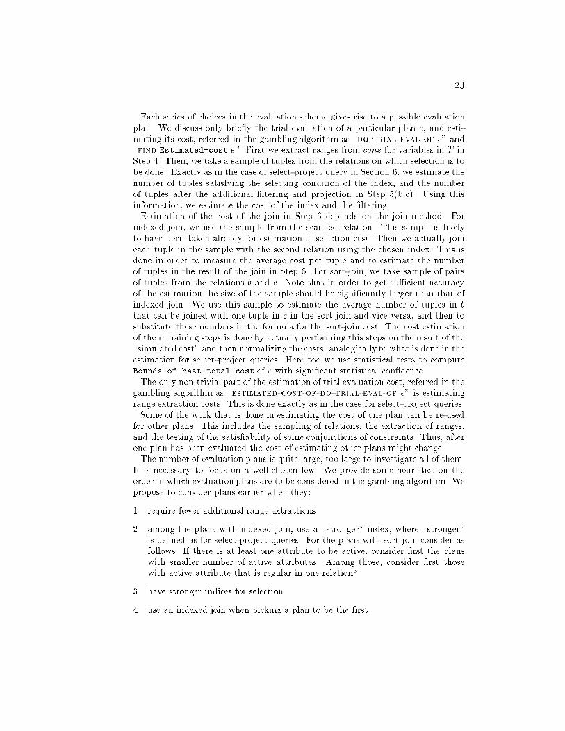
23Each series of choices in the evaluation scheme gives rise to a possible evaluationplan. We discuss only brie y the trial evaluation of a particular plan e, and esti-mating its cost, referred in the gambling algorithm as \do-trial-eval-of e" and\find Estimated-cost.e." First we extract ranges from cons for variables in T inStep 4. Then, we take a sample of tuples from the relations on which selection is tobe done. Exactly as in the case of select-project query in Section 6, we estimate thenumber of tuples satisfying the selecting condition of the index, and the numberof tuples after the additional �ltering and projection in Step 5(b,c). Using thisinformation, we estimate the cost of the index and the �ltering.Estimation of the cost of the join in Step 6 depends on the join method. Forindexed join, we use the sample from the scanned relation. This sample is likelyto have been taken already for estimation of selection cost. Then we actually joineach tuple in the sample with the second relation using the chosen index. This isdone in order to measure the average cost per tuple and to estimate the numberof tuples in the result of the join in Step 6. For sort-join, we take sample of pairsof tuples from the relations b and c. Note that in order to get su�cient accuracyof the estimation the size of the sample should be signi�cantly larger than that ofindexed join. We use this sample to estimate the average number of tuples in bthat can be joined with one tuple in c in the sort join and vice versa, and then tosubstitute these numbers in the formula for the sort-join cost. The cost estimationof the remaining steps is done by actually performing this steps on the result of the\simulated cost" and then normalizing the costs, analogically to what is done in theestimation for select-project queries. Here too we use statistical tests to computeBounds-of-best-total-cost of e with signi�cant statistical con�dence.The only non-trivial part of the estimation of trial evaluation cost, referred in thegambling algorithm as \estimated-cost-of-do-trial-eval-of e" is estimatingrange extraction costs. This is done exactly as in the case for select-project queries.Some of the work that is done in estimating the cost of one plan can be re-usedfor other plans. This includes the sampling of relations, the extraction of ranges,and the testing of the satis�ability of some conjunctions of constraints. Thus, afterone plan has been evaluated the cost of estimating other plans might change.The number of evaluation plans is quite large, too large to investigate all of them.It is necessary to focus on a well-chosen few. We provide some heuristics on theorder in which evaluation plans are to be considered in the gambling algorithm. Wepropose to consider plans earlier when they:1. require fewer additional range extractions.2. among the plans with indexed join, use a \stronger" index, where \stronger"is de�ned as for select-project queries. For the plans with sort join consider asfollows. If there is at least one attribute to be active, consider �rst the planswith smaller number of active attributes. Among those, consider �rst thosewith active attribute that is regular in one relation6.3. have stronger indices for selection.4. use an indexed join when picking a plan to be the �rst.

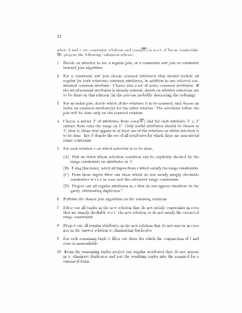
22where b and c are constraint relations and cons(W ) is a set of linear constraints.We propose the following evaluation scheme:1. Decide on whether to use a regular join, or a constraint sort join or constraintindexed join algorithm.2. For a constraint sort join choose scanned attributes that should include allregular (in both relations) common attributes, in addition to one selected con-strained common attribute. Choose also a set of active common attributes. Ifthe set of scanned attributes is already ordered, decide on whether selections areto be done on this relation (in the process probably destroying the ordering).3. For an index join, decide which of the relations is to be scanned, and choose anindex on common attribute(s) for the other relation. The selections before thejoin will be done only on the scanned relation.4. Choose a subset T of attributes from cons(W ) and for each attribute V 2 Textract from cons the range on V . Only useful attributes should be chosen inT , that is, those that appear in at least one of the relations on which selection isto be done. Let S denote the set of all attributes for which there are non-trivialrange constraint.5. For each relation r on which selection is to be done,(A) Pick an index whose selection condition can be explicitly checked by therange constraints on attributes in S.(B) Using this index, select all tuples from r which satisfy the range constraints.(C) From these tuples �lter out those which do not satisfy simply checkableconstraints w.r.t r in cons and the extracted range constraints.(D) Project out all regular attributes in r that do not appear elsewhere in thequery, eliminating duplicates.56. Perform the chosen join algorithm on the resulting relations.7. Filter out all tuples in the new relation that do not satisfy constraints in consthat are simply checkable w.r.t. the new relation, or do not satisfy the extractedrange constraints.8. Project out all regular attributes in the new relation that do not appear in consnor in the answer relation a, eliminating duplicates.9. For each remaining tuple t, �lter out those for which the conjunction of t andcons is unsatis�able.10. From the remaining tuples project out regular attributes that do not appearin a, eliminate duplicates and put the resulting tuples into the required for acanonical form;

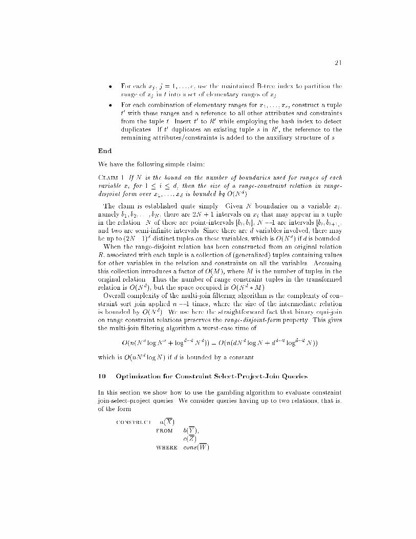
21� For each xj, j = 1; : : : ; e, use the maintained B-tree index to partition therange of xj in t into a set of elementary ranges of xj� For each combination of elementary ranges for x1; : : : ; xe, construct a tuplet0 with these ranges and a reference to all other attributes and constraintsfrom the tuple t. Insert t0 to R0 while employing the hash index to detectduplicates. If t0 duplicates an existing tuple s in R0, the reference to theremaining attributes/constraints is added to the auxiliary structure of s.EndWe have the following simple claim:Claim 1 If N is the bound on the number of boundaries used for ranges of eachvariable xi for 1 � i � d, then the size of a range-constraint relation in range-disjoint form over x1; : : : ; xd is bounded by O(Nd).The claim is established quite simply. Given N boundaries on a variable xi,namely b1; b2; : : : ; bN , there are 2N + 1 intervals on xi that may appear in a tuplein the relation. N of these are point-intervals [bi; bi], N � 1 are intervals [bi; bi+1],and two are semi-in�nite intervals. Since there are d variables involved, there maybe up to (2N+1)d distinct tuples on these variables, which is O(Nd) if d is bounded.When the range-disjoint relation has been constructed from an original relationR, associated with each tuple is a collection of (generalized) tuples containing valuesfor other variables in the relation and constraints on all the variables. Accessingthis collection introduces a factor of O(M ), where M is the number of tuples in theoriginal relation. Thus the number of range constraint tuples in the transformedrelation is O(Nd), but the space occupied is O(Nd �M ).Overall complexity of the multi-join �ltering algorithm is the complexity of con-straint sort join applied n � 1 times, where the size of the intermediate relationis bounded by O(Nd). We use here the straightforward fact that binary equi-joinon range constraint relations preserves the range-disjoint-form property. This givesthe multi-join �ltering algorithm a worst-case time ofO(n(Nd logNd + logd�2Nd)) = O(n(dNd logN + dd�2 logd�2N ))which is O(nNd logN ) if d is bounded by a constant.10. Optimization for Constraint Select-Project-Join QueriesIn this section we show how to use the gambling algorithm to evaluate constraintjoin-select-project queries. We consider queries having up to two relations, that is,of the formconstruct a(X)from b(Y );c(Z)where cons(W )

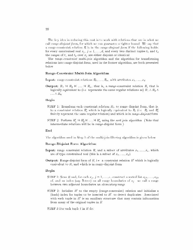
20The key idea in reducing this cost is to work with relations that are in what wecall range-disjoint form, for which we can guarantee a tighter bound. We say thata range-constraint relation R is in the range-disjoint form if the following holds:for every constrained real xj, j = 1; : : : ; d, and every two distinct tuples t1 and t2the ranges of t1 and t2 over xj are either disjoint or identical.The range-constraint multi-join algorithm and the algorithm for transformingrelations into range-disjoint form, used in the former algorithm, are both presentedbelow.Range-Constraint Multi-Join AlgorithmInput: range-constraint relations R1; : : : ; Rn, with attributes x1; : : : ; xd.Output: R1 1 R2 1 : : : 1 Rn, that is, a range-constraint relation R, that islogically equivalent to (i.e. represents the same regular relations as) R1 ^R2 ^: : :^Rn.BeginSTEP 1: Transform each constraint relation Ri, to range disjoint form, that is,to a constraint relation R0i which is logically equivalent to Ri (i.e. Ri and R0i�nitely represent the same regular relation) and which is in range-disjoint form.STEP 2: Perform R01 1 R02 1 : : : 1 R0n using the sort join algorithm. (Note thatintermediate relations will be in range-disjoint form.)EndThe algorithm used in Step 1 of the multi-join �ltering algorithm is given below.Range-Disjoint Form AlgorithmInput: range constraint relation R, and a subset of attributes x1; : : : ; xe, whichare of type constrained real (this is a subset of x1; : : : ; xd)Output: Range-disjoint form of R, i.e. a constraint relation R0 which is logicallyequivalent to R, and which is in range-disjoint form.BeginSTEP 1: Scan R and, for each xj, j = 1; : : : ; e, construct a sorted list aj1; : : : ; ajkof, and an index (say B-tree) on all range boundaries of xj. we call a rangebetween two adjacent boundaries an elementary range.STEP 2: Intialize R0 to the empty (range-constraint) relation and initialize a(hash) index for tuples to be inserted to R0, to detect duplicates. Associatedwith each tuple in R0 is an auxiliary structure that may contain informationfrom many of the original tuples in R.STEP 3 For each tuple t in R do:

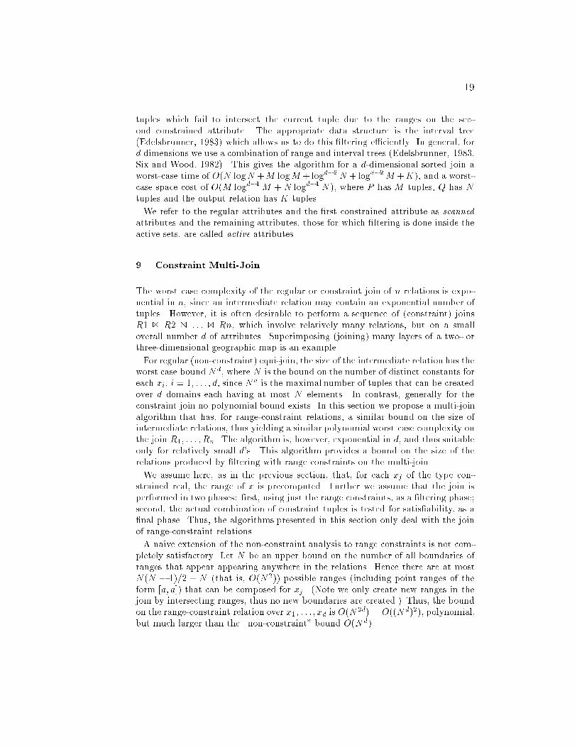
19tuples which fail to intersect the current tuple due to the ranges on the sec-ond constrained attribute. The appropriate data structure is the interval tree(Edelsbrunner, 1983) which allows us to do this �ltering e�ciently. In general, ford dimensions we use a combination of range and interval trees (Edelsbrunner, 1983,Six and Wood, 1982). This gives the algorithm for a d-dimensional sorted join aworst-case time of O(N logN +M logM +logd�2N +logd�2M +K), and a worst-case space cost of O(M logd�1M + N logd�1N ), where P has M tuples, Q has Ntuples and the output relation has K tuples.We refer to the regular attributes and the �rst constrained attribute as scannedattributes and the remaining attributes, those for which �ltering is done inside theactive sets, are called active attributes.9. Constraint Multi-JoinThe worst case complexity of the regular or constraint join of n relations is expo-nential in n, since an intermediate relation may contain an exponential number oftuples. However, it is often desirable to perform a sequence of (constraint) joinsR1 1 R2 1 : : : 1 Rn, which involve relatively many relations, but on a smalloverall number d of attributes. Superimposing (joining) many layers of a two- orthree-dimensional geographic map is an example.For regular (non-constraint) equi-join, the size of the intermediate relation has theworst case bound Nd, where N is the bound on the number of distinct constants foreach xi, i = 1; : : : ; d, since Nd is the maximal number of tuples that can be createdover d domains each having at most N elements. In contrast, generally for theconstraint join no polynomial bound exists. In this section we propose a multi-joinalgorithm that has, for range-constraint relations, a similar bound on the size ofintermediate relations, thus yielding a similar polynomial worst case complexity onthe join R1; : : : ; Rn. The algorithm is, however, exponential in d, and thus suitableonly for relatively small d's. This algorithm provides a bound on the size of therelations produced by �ltering with range constraints on the multi-join.We assume here, as in the previous section, that, for each xj of the type con-strained real, the range of x is precomputed. Further we assume that the join isperformed in two phases: �rst, using just the range constraints, as a �ltering phase;second, the actual combination of constraint tuples is tested for satis�ability, as a�nal phase. Thus, the algorithms presented in this section only deal with the joinof range-constraint relations.A naive extension of the non-constraint analysis to range constraints is not com-pletely satisfactory. Let N be an upper bound on the number of all boundaries ofranges that appear appearing anywhere in the relations. Hence there are at mostN (N � 1)=2 + N (that is, O(N2)) possible ranges (including point ranges of theform [a; a]) that can be composed for xj. (Note we only create new ranges in thejoin by intersecting ranges, thus no new boundaries are created.) Thus, the boundon the range-constraint relation over x1; : : : ; xd is O(N2d) = O((Nd)2), polynomial,but much larger than the \non-constraint" bound O(Nd).

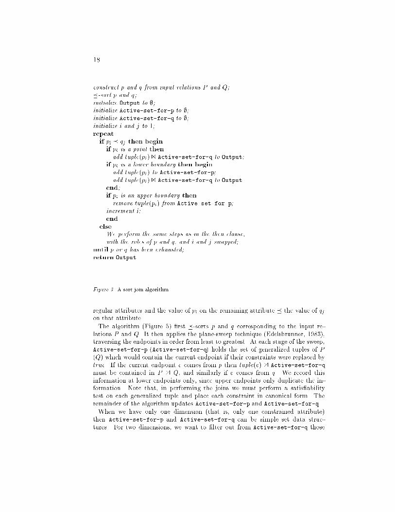
18construct p and q from input relations P and Q;�-sort p and q;initialize Output to ;;initialize Active-set-for-p to ;;initialize Active-set-for-q to ;;initialize i and j to 1;repeatif pi � qj then beginif pi is a point thenadd tuple(pi) 1 Active-set-for-q to Output;if pi is a lower boundary then beginadd tuple(pi) to Active-set-for-p;add tuple(pi) 1 Active-set-for-q to Outputend;if pi is an upper boundary thenremove tuple(pi) from Active-set-for-p;increment i;endelseWe perform the same steps as in the then clause,with the roles of p and q, and i and j swapped;until p or q has been exhausted;return OutputFigure 5. A sort join algorithmregular attributes and the value of pi on the remaining attribute � the value of qjon that attribute.The algorithm (Figure 5) �rst �-sorts p and q corresponding to the input re-lations P and Q. It then applies the plane-sweep technique (Edelsbrunner, 1983),traversing the endpoints in order from least to greatest. At each stage of the sweep,Active-set-for-p (Active-set-for-q) holds the set of generalized tuples of P(Q) which would contain the current endpoint if their constraints were replaced bytrue. If the current endpoint e comes from p then tuple(e) 1 Active-set-for-qmust be contained in P 1 Q, and similarly if e comes from q. We record thisinformation at lower endpoints only, since upper endpoints only duplicate the in-formation. Note that, in performing the joins we must perform a satis�abilitytest on each generalized tuple and place each constraint in canonical form. Theremainder of the algorithm updates Active-set-for-p and Active-set-for-q.When we have only one dimension (that is, only one constrained attribute)then Active-set-for-p and Active-set-for-q can be simple set data struc-tures. For two dimensions, we want to �lter out from Active-set-for-q those

17let ebest 2 Best-eval-plans be the plan that has the least estimated cost;set Spent-cost to 0;while size of Best-eval-plans > 1 do beginfor each plan e0, except ebest, compute statistical con�dence Ce0 with which the cost of e0exceeds the cost of ebest minus " percent; suppose Ce is the lowest;discard all plans e0 in Best-eval-plans with Ce0 � SIGNIFICANT CONFIDENCE;compute Max-trials-cost as a function ofEstimated-cost.ebest and Bounds-of-estimated-cost.ebest;set One-trial-cost to Max-trials-cost = MAX-ITERATIONS;if One-trial-cost > Max-trials-cost � Spent-cost thendiscard all plans but ebest from Best-eval-planselse beginincrement Spent-cost by One-trial-cost;evaluate-optimal-partition-of One-trial-cost giving costs Cost1 and Cost2of work to be spent on estimating costs of ebest and e respectively;take additional samples for estimating costs of ebest and e spendingCost1 and Cost2 respectively and re-estimate the costs of ebest and e;if Estimated-cost.ebest > Estimated-cost.e thenset ebest to e;endendreturn ebestFigure 4. Procedure choose-best-plan

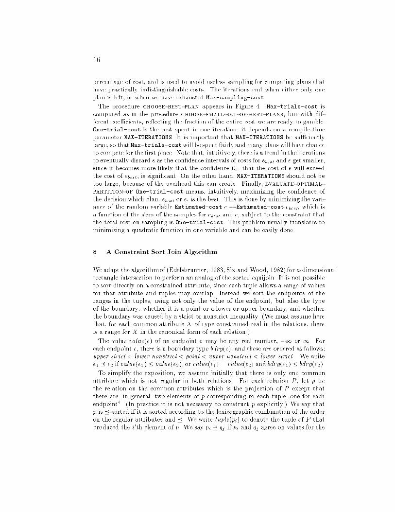
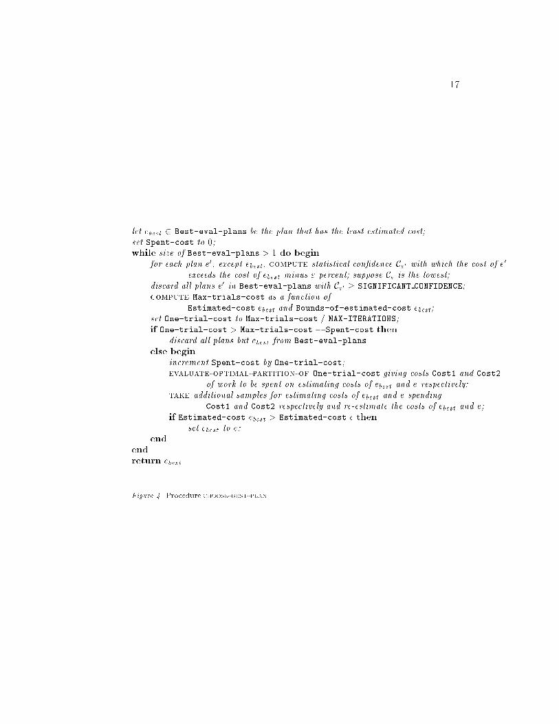
16percentage of cost, and is used to avoid useless sampling for comparing plans thathave practically indistinguishable costs. The iterations end when either only oneplan is left, or when we have exhausted Max-sampling-cost.The procedure choose-best-plan appears in Figure 4. Max-trials-cost iscomputed as in the procedure choose-small-set-of-best-plans, but with dif-ferent coe�cients, re ecting the fraction of the entire cost we are ready to gamble.One-trial-cost is the cost spent in one iteration; it depends on a compile-timeparameter MAX-ITERATIONS. It is important that MAX-ITERATIONS be su�cientlylarge, so that Max-trials-costwill be spent fairly and many plans will have chanceto compete for the �rst place. Note that, intuitively, there is a trend in the iterationsto eventually discard e as the con�dence intervals of costs for ebest and e get smaller,since it becomes more likely that the con�dence Ce, that the cost of e will exceedthe cost of ebest, is signi�cant. On the other hand, MAX-ITERATIONS should not betoo large, because of the overhead this can create. Finally, evaluate-optimal-partition-of One-trial-cost means, intuitively, maximizing the con�dence ofthe decision which plan, ebest or e, is the best. This is done by minimizing the vari-ance of the random variable Estimated-cost.e � Estimated-cost.ebest, which isa function of the sizes of the samples for ebest and e, subject to the constraint thatthe total cost on sampling is One-trial-cost. This problem usually translates tominimizing a quadratic function in one variable and can be easily done.8. A Constraint Sort Join AlgorithmWe adapt the algorithmof (Edelsbrunner, 1983, Six and Wood, 1982) for n-dimensionalrectangle intersection to perform an analog of the sorted equijoin. It is not possibleto sort directly on a constrained attribute, since each tuple allows a range of valuesfor that attribute and tuples may overlap. Instead we sort the endpoints of theranges in the tuples, using not only the value of the endpoint, but also the typeof the boundary: whether it is a point or a lower or upper boundary, and whetherthe boundary was caused by a strict or nonstrict inequality. (We must assume herethat, for each common attribute X of type constrained real in the relations, thereis a range for X in the canonical form of each relation.)The value value(e) of an endpoint e may be any real number, �1 or 1. Foreach endpoint e, there is a boundary type bdry(e), and these are ordered as follows:upper-strict < lower-nonstrict < point < upper-nonstrict < lower-strict. We writee1 � e2 if value(e1) � value(e2), or value(e1) = value(e2) and bdry(e1) � bdry(e2).To simplify the exposition, we assume initially that there is only one commonattribute which is not regular in both relations. For each relation P , let p bethe relation on the common attributes which is the projection of P except thatthere are, in general, two elements of p corresponding to each tuple, one for eachendpoint4. (In practice it is not necessary to construct p explicitly.) We say thatp is �-sorted if it is sorted according to the lexicographic combination of the orderon the regular attributes and �. We write tuple(pi) to denote the tuple of P thatproduced the i'th element of p. We say pi � qj if pi and qj agree on values for the

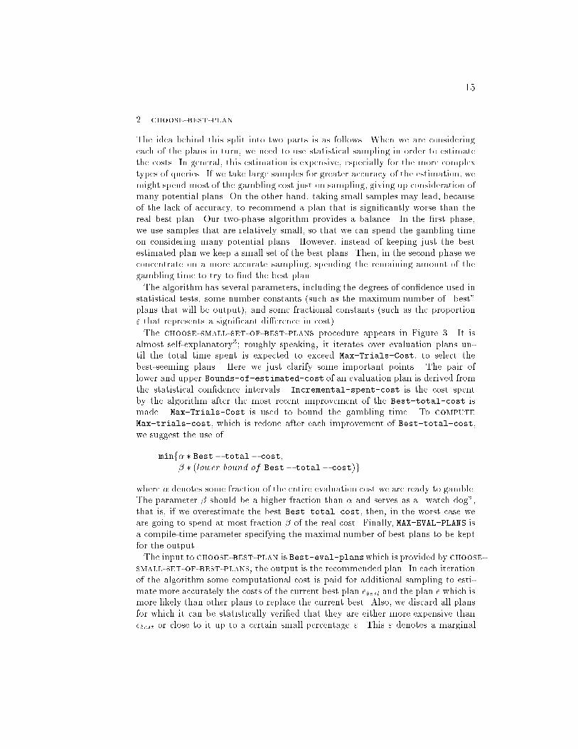
152. choose-best-planThe idea behind this split into two parts is as follows. When we are consideringeach of the plans in turn, we need to use statistical sampling in order to estimatethe costs. In general, this estimation is expensive, especially for the more complextypes of queries. If we take large samples for greater accuracy of the estimation, wemight spend most of the gambling cost just on sampling, giving up consideration ofmany potential plans. On the other hand, taking small samples may lead, becauseof the lack of accuracy, to recommend a plan that is signi�cantly worse than thereal best plan. Our two-phase algorithm provides a balance. In the �rst phase,we use samples that are relatively small, so that we can spend the gambling timeon considering many potential plans. However, instead of keeping just the bestestimated plan we keep a small set of the best plans. Then, in the second phase weconcentrate on a more accurate sampling, spending the remaining amount of thegambling time to try to �nd the best plan.The algorithm has several parameters, including the degrees of con�dence used instatistical tests, some number constants (such as the maximum number of \best"plans that will be output), and some fractional constants (such as the proportion" that represents a signi�cant di�erence in cost).The choose-small-set-of-best-plans procedure appears in Figure 3. It isalmost self-explanatory3; roughly speaking, it iterates over evaluation plans un-til the total time spent is expected to exceed Max-Trials-Cost, to select thebest-seeming plans. Here we just clarify some important points. The pair oflower and upper Bounds-of-estimated-cost of an evaluation plan is derived fromthe statistical con�dence intervals. Incremental-spent-cost is the cost spentby the algorithm after the most recent improvement of the Best-total-cost ismade. Max-Trials-Cost is used to bound the gambling time. To computeMax-trials-cost, which is redone after each improvement of Best-total-cost,we suggest the use ofminf� � Best� total� cost;� � (lower bound of Best� total� cost)gwhere � denotes some fraction of the entire evaluation cost we are ready to gamble.The parameter � should be a higher fraction than � and serves as a \watch dog",that is, if we overestimate the best Best-total-cost, then, in the worst case weare going to spend at most fraction � of the real cost. Finally, MAX-EVAL-PLANS isa compile-time parameter specifying the maximal number of best plans to be keptfor the output.The input to choose-best-plan is Best-eval-planswhich is provided by choose-small-set-of-best-plans; the output is the recommended plan. In each iterationof the algorithm some computational cost is paid for additional sampling to esti-mate more accurately the costs of the current best plan ebest and the plan e which ismore likely than other plans to replace the current best. Also, we discard all plansfor which it can be statistically veri�ed that they are either more expensive thanebest or close to it up to a certain small percentage ". This " denotes a marginal

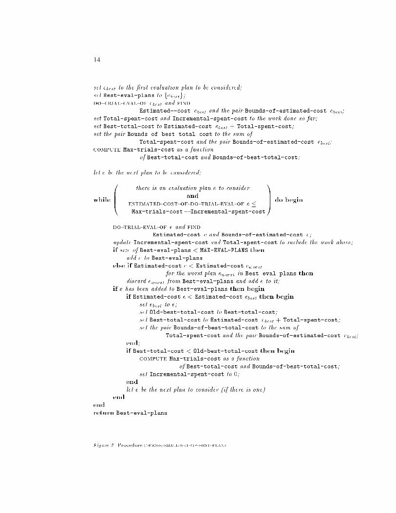
14set ebest to the �rst evaluation plan to be considered;set Best-eval-plans to febestg;do-trial-eval-of ebest and findEstimated--cost.ebest and the pair Bounds-of-estimated-cost.ebest;set Total-spent-cost and Incremental-spent-cost to the work done so far;set Best-total-cost to Estimated-cost.ebest + Total-spent-cost;set the pair Bounds-of-best-total-cost to the sum ofTotal-spent-cost and the pair Bounds-of-estimated-cost.ebest;compute Max-trials-cost as a functionof Best-total-cost and Bounds-of-best-total-cost;let e be the next plan to be considered;while 0BB@ there is an evaluation plan e to considerandestimated-cost-of-do-trial-eval-of e �Max-trials-cost� Incremental-spent-cost1CCA do begindo-trial-eval-of e and findEstimated-cost.e and Bounds-of-estimated-cost.e;update Incremental-spent-cost and Total-spent-cost to include the work above;if size of Best-eval-plans < MAX-EVAL-PLANS thenadd e to Best-eval-planselse if Estimated-cost.e < Estimated-cost.eworstfor the worst plan eworst in Best-eval-plans thendiscard eworst from Best-eval-plans and add e to it;if e has been added to Best-eval-plans then beginif Estimated-cost.e < Estimated-cost.ebest then beginset ebest to e;set Old-best-total-cost to Best-total-cost;set Best-total-cost to Estimated-cost.ebest + Total-spent-cost;set the pair Bounds-of-best-total-cost to the sum ofTotal-spent-cost and the pair Bounds-of-estimated-cost.ebest;end;if Best-total-cost < Old-best-total-cost then begincompute Max-trials-cost as a functionof Best-total-cost and Bounds-of-best-total-cost;set Incremental-spent-cost to 0;endlet e be the next plan to consider (if there is one)endendreturn Best-eval-plansFigure 3. Procedure choose-small-set-of-best-plans

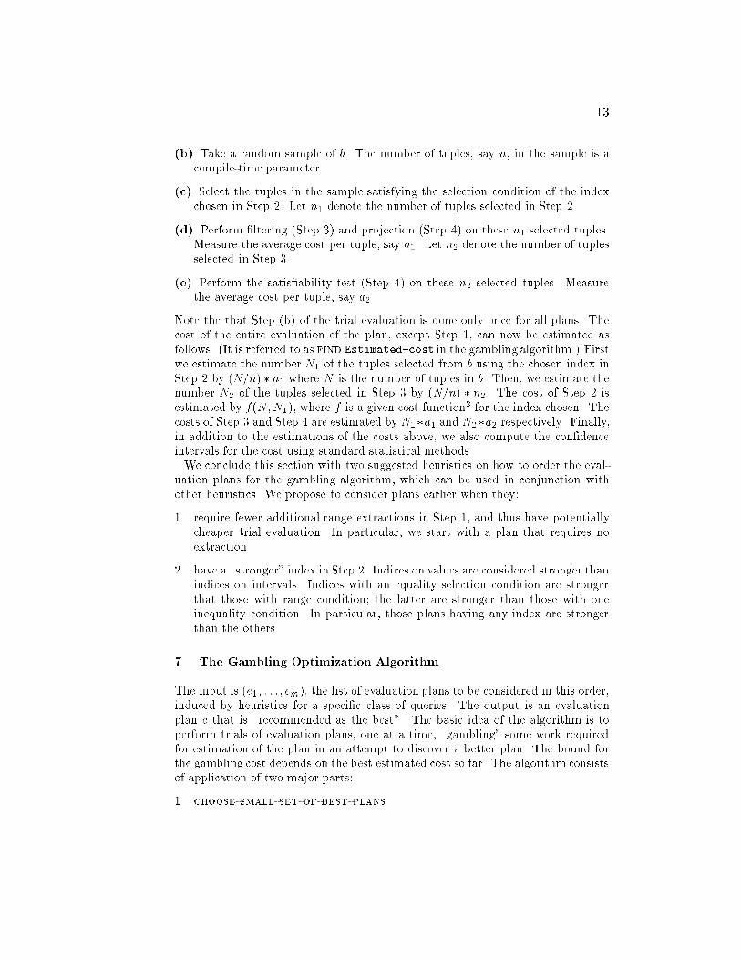
13(b) Take a random sample of b. The number of tuples, say n, in the sample is acompile-time parameter.(c) Select the tuples in the sample satisfying the selection condition of the indexchosen in Step 2. Let n1 denote the number of tuples selected in Step 2.(d) Perform �ltering (Step 3) and projection (Step 4) on these n1 selected tuples.Measure the average cost per tuple, say a1. Let n2 denote the number of tuplesselected in Step 3.(e) Perform the satis�ability test (Step 4) on these n2 selected tuples. Measurethe average cost per tuple, say a2.Note the that Step (b) of the trial evaluation is done only once for all plans. Thecost of the entire evaluation of the plan, except Step 1, can now be estimated asfollows. (It is referred to as find Estimated-cost in the gambling algorithm.) Firstwe estimate the number N1 of the tuples selected from b using the chosen index inStep 2 by (N=n) � n1 where N is the number of tuples in b. Then, we estimate thenumber N2 of the tuples selected in Step 3 by (N=n) � n2. The cost of Step 2 isestimated by f(N;N1), where f is a given cost function2 for the index chosen. Thecosts of Step 3 and Step 4 are estimated by N1�a1 and N2�a2 respectively. Finally,in addition to the estimations of the costs above, we also compute the con�denceintervals for the cost using standard statistical methods.We conclude this section with two suggested heuristics on how to order the eval-uation plans for the gambling algorithm, which can be used in conjunction withother heuristics. We propose to consider plans earlier when they:1. require fewer additional range extractions in Step 1, and thus have potentiallycheaper trial evaluation. In particular, we start with a plan that requires noextraction.2. have a \stronger" index in Step 2. Indices on values are considered stronger thanindices on intervals. Indices with an equality selection condition are strongerthat those with range condition; the latter are stronger than those with oneinequality condition. In particular, those plans having any index are strongerthan the others.7. The Gambling Optimization AlgorithmThe input is (e1; : : : ; em), the list of evaluation plans to be considered in this order,induced by heuristics for a speci�c class of queries. The output is an evaluationplan e that is \recommended as the best". The basic idea of the algorithm is toperform trials of evaluation plans, one at a time, \gambling" some work requiredfor estimation of the plan in an attempt to discover a better plan. The bound forthe gambling cost depends on the best estimated cost so far. The algorithm consistsof application of two major parts:1. choose-small-set-of-best-plans

12work that needs to be done. We then discuss the trial evaluation, which is necessaryfor estimating costs, and some heuristics which can be used to order evaluationplans. The generic gambling algorithm, described in the next section, uses thisinformation to choose which plans receive a trial evaluation and, ultimately, tochoose an evaluation plan.We propose the following evaluation scheme for this query.0. If Z \W is empty then no selection is involved. Project b onto Y , eliminat-ing duplicates, and conjoin the constraint in each generalized tuple with theprojection of cons(W ) onto Y .1. Choose a non-empty subset T of the common attributes Z\W . For eachX 2 T ,extract from cons a range on X. Let S be the set of all attributes in Z [W forwhich there are non-trivial range constraints (including those attributes fromT ).2. Pick an index maintained on b whose selection condition can be explicitlychecked by the range constraints on attributes in S. Using this index, select alltuples from b satisfying the constraints.3. From these tuples, �lter out those which do not satisfy simply checkable con-straints from cons and the extracted range constraints.4. Project out all regular attributes of b that do not appear elsewhere, eliminatingduplicates.5. For each remaining tuple t, check the satis�ability of the conjunction of t andcons. If it is satis�able, put it in canonical form. If it is not, discard it.This scheme leaves open the speci�c choice of a subset T of variables, and an index.Fixing a choice gives rise to a particular evaluation plan.The cost of an evaluation plan depends strongly on the ranges extracted in Step 1.Therefore, the estimation of such cost requires, in addition to statistical sampling,some amount of actual evaluation. Call this process of sampling/evaluation a trialevaluation of the plan. Now, even trial evaluation can be expensive and thereforeit is unrealistic to estimate the cost of all evaluation plans. In fact the cost ofestimation may exceed the cost of a naive evaluation.In the next section, we provide our gambling algorithm that balances these twocosts by considering evaluations plans one at a time and limiting the cost of theestimation of a plan to a portion of the cost of the best plan according to theestimation so far. For the remainder of this section, we detail the trial evaluationand provide heuristics on the order in which the plans are to be considered forestimation.The trial evaluation for a given plan is described by steps (a) { (e) below. Thesesteps comprise the sub-procedure do-trial-eval-of of the gambling algorithm forthe case of selection-projection queries. (We provide di�erent steps for other kindsof queries later.)(a) Perform Step 1 above.

11construct a(X1; : : : ; Xi; : : : ; Xj; : : : ; Xn)from b(X1; : : : ; Xj);c(Xi; : : : ; Xn)In principle, each tuple in the answer to this query can be computed by takinga conjunction of a tuple from b and a tuple from c, testing its satis�ability and,if satis�able, presenting it in the required canonical form. As with the constraintselection, we can use �ltering to reduce the cost of satis�ability tests. The �lteringstep discards those pairs of tuples that have disjoint ranges on a common attribute.A re�nement step then performs a full test for satis�ability for the remaining pairs.Note that the regular join does not involve constraints and hence does not requirethe re�nement step. In this paper, we associate the notion of join only with the�ltering step, and treat the full test for satis�ability as a separate operation.We would like to use the ideas developed for regular joins for the �ltering in theconstraint join. The indexed join (that is, for each tuple of one relation �nding allcorresponding tuples of the second using an index) for constraint relations di�ersfrom the indexed join for regular relations only in the di�erent index structuresthat can be used. However, an analogy for the sort join (sorting both relationson common attributes and then �nding all matching tuples in one merge) is notclear, since there is no appropriate total ordering on multidimensional intervals. InSection 8 we adapt work in computational geometry to give an analog to the sortjoin.Finally, consider the two major approaches to query optimization for regulardatabases. One is based on algebraic simpli�cation of a query and compile-timeheuristics. The other is based on cost estimation of di�erent strategies. Neitherof these is adequate for constraint database systems. The heuristics of the alge-braic approach, such as performing selections as early as possible, are based onthe assumption that selection conditions are readily available. In contrast, extract-ing such conditions from the constraints of a query involves linear programmingtechniques which are in general expensive. For the cost estimation approach, wehave a similar problem of extracting explicit constraints which are needed for theestimation. Even if these constraints were readily available, there is a second prob-lem: it is typically necessary to make assumptions about distribution of the data(like uniformity within, and independence of, columns) in the database, and theseappear unlikely to hold in constraint databases.6. Algorithm for Constraint Selection and ProjectionHere the considered queries are of the formconstruct a(Y )from b(Z)where cons(W )We proceed by presenting an evaluation scheme which represents many evaluationplans. Evaluation schemes and plans are not intended to represent the decision-making process, but only to represent the decisions that need to be made, and the

10canonical form for tuples of r. While testing such a constraint is a little moreexpensive, in general, than testing ranges, the cost still compares very favorablywith the use of linear programming.)We can do �ltering more e�ciently using indices. Indexing on regular attributesis the same as usual, whereas indexing on a constraint attribute X of r works asfollows. For each inserted constraint tuple t the range of X is extracted usinglinear programming techniques. This interval is inserted into an index structuremaintaining intervals and has a reference to the corresponding tuple. Selection of alltuples t in r consistent with a given set of constraints c is done as follows. First therange I of X is extracted from c. Second, using the interval index all tuples whosecorresponding ranges of X intersect I are retrieved. Third, the retrieved tuplesare checked for consistency with c using linear programming methods. Of course,many di�erent indices can be maintained and used for selection. Moreover, in orderto improve �ltering additional attributes can be de�ned as linear combinations ofconstraint attributes, as proposed in (Brodsky et al., 1995).In general we need to have index structures supporting storage of values andintervals, and value and range queries. Two e�cient access structures for in-tervals are the interval tree (Edelsbrunner, 1983) and the priority search trees(McCreight, 1985). In one dimension, �nding all intervals intersecting a given in-terval or containing a given point, takes at most O(n log n + k) time, where nis the size of the relation and k is the size of the output. Moreover, it requiresonly linear space in the size of a relation, and thus seems to be ideal as an in-dexing structure. The work in (Kanellakis et al., 1993) proposes an e�cient datastructure for secondary storage, having the same space and time complexity andfull clustering. There are di�erent data structures to support access to multidi-mensional intervals, in particular based on combination of interval, segment andrange trees (Edelsbrunner, 1983, Six and Wood, 1982). For 2-dimensional inter-vals (rectangles) R, R+, R�trees (Guttman, 1984, Roussopoulos and Leifker, 1985,Sellis et al., 1987) are widely used in spatial databases.In order to perform indexing and �ltering, it is necessary to extract ranges ofvariables from cons. This extraction involves techniques of linear programming andcan be very expensive, especially in applications coming from operational researchin which cons might involve over a thousand constraints and variables. Thus, thereis a trade-o� to be made between an improvement gained by �ltering and indexingand the cost paid for extracting ranges from cons.Consider now projections, that is, the queries of the formconstruct a(X1; : : : ; Xn)from b(X1; : : : ; Xn; : : : ; Xm)Computing a projection may involve, depending on the required canonical form,quanti�er elimination of (some of) the variables Xn+1; : : : ; Xm. In contrast to theusual database case, in which projection is a trivial operation, when constraints areinvolved it can be computationally expensive.Consider now a \constraint" join, where the query is of the form

9�1 < X or X <1.) More speci�cally, we require the \tightest" such range, whichcan be obtained for each variable by projecting the conjunctive constraint ontothe variable. Placing constraints in canonical form and, in particular, testing thesatis�ability (or consistency) of constraints requires, in general, linear programmingtechniques.For the purposes of this paper we consider just one class of canonical forms.We assume that there are no implicit equations, that equations are presented inparameterized form (as described in the �rst choice above), some simple redundancyin the inequalities is removed, and there are explicit range constraints for somevariables.In addition to choosing canonical forms for constraint relations, we must alsoconsider the manipulations of constraints necessary in the evaluation of queries.The most important computation with query constraints is the extraction of arange on a variable. The extraction of a lower bound (for example) on x is exactlythe linear programming problem of minimizing x subject to the constraints. Thedetection of implicit equalities in the query constraint is also a linear programmingproblem (Lassez, 1990) as is, of course, testing for consistency.5. Optimization: Di�erences in ApproachIn this section we highlight di�erences between constraint databases and regulardatabases, which make the straightforward application of usual database techniquesdi�cult or impossible. Consider, �rst, a simple problem of selection, that is, thequery of the formconstruct a(X1; : : : ; Xn)from b(X1; : : : ; Xi; : : : ; Xn)where cons(Xi; : : : ; Xn; : : : ; Xm)Each constraint tuple of a can be constructed by taking a conjunction of a constrainttuple from b and cons, testing whether it is satis�able, and if it is, �nding a requiredcanonical form for it. Note that, depending on the canonical form for existentialquanti�ers, this may involve elimination of the implicit existential quanti�ers overthe variables Xn+1; : : : ; Xm. Thus, in general, processing a tuple in a constraintselection is signi�cantly more expensive than in a regular selection.To avoid unnecessary computation, we want to use the idea of �ltering, similar toone used in spatial databases, that is, the discarding of irrelevant tuples of b by acomputationally cheap test. Suppose we have a range c � Xk < d for Xk in cons,where c might be �1 and d might be 1. If Xk is also a regular variable in b, wecan discard all tuples in b whose Xk value does not lie in the range, since clearlythose tuples are inconsistent with cons. Similarly, if Xk is a constrained variableand a range for Xk is stored for each tuple of b, then we can discard all tuples forwhich the ranges for Xk are disjoint.(There is a larger class of constraints of use in �ltering. A constraint is simplycheckable wrt a relation r if every variable in the constraint also occurs in therelation in an attribute that either is regular or has a range constraint in the

8 Instead we direct our attention to a subset of this query language in which allconstraints appearing in a query are linear. We consider selections and projectionsof relations, and the join of two relations, but we do not explicitly discuss the unionoperation.4. Canonical Forms and Constraint ManipulationIn this paper, the constraint c associated with a constraint tuple is a (possiblyexistentially quanti�ed) conjunction of linear equations and inequalities. In thissection, we brie y discuss some computational issues on the manipulation of suchconstraints.A canonical form for constraints is a useful standard form of the constraints, andis generally computed by simpli�cation and the removal of redundancy. In additionto the advantages of a standard presentation of constraints, canonical forms canprovide savings of space and time. In the class of linear arithmetic constraints thereare many plausible canonical forms. However, they can be costly to compute.Corresponding to a constraint relation is a disjunction of the constraints in eachtuple. Some of these tuples might be redundant in the sense that omitting themdoes not alter the regular relation represented by the constraint relation. Clearly,a canonical form that eliminates such tuples would be desirable. However, theproblem of detecting such tuples is co-NP-complete (Srivastava, 1992), and so wewill perform only two simpli�cations of disjunctions: the deletion of each tuplewith an inconsistent constraint, and the deletion of duplicates when all values areregular.Similarly, while it is theoretically possible to eliminate all existential quanti�ersfrom our constraints (as required in the framework of (Kanellakis et al., 1990)), thecost of this elimination and the size of the resulting constraint can grow exponen-tially in the size of the original constraint. Since we expect applications with largeconstraints, it is unrealistic to expect that all quanti�ers can be eliminated. Wesuggest a method of only performing simplifying quanti�er eliminations, similar towhat is done in CLP(R) (Ja�ar et al., 1993).The conjunctive constraints o�er the greatest scope in choosing a canonical form.One choice is to write all equations in the form fxi = ti j i = 1; : : : ; ng where thexi's are distinct and appear nowhere else in the constraint (parameterized form).A second choice is whether all equations which are implicit in the inequality con-straints should be represented explicitly. (As a simple example of this, consider theconstraints x+y � 2; x+y � 2.) A third is the extent to which redundancy withinthe inequalities should be removed. (Lassez et al., 1989) presents a classi�cation ofredundancy that suggests simple forms of redundancy removal. A fourth choice iswhether to keep the inequalities in a di�erent form, such as simplex tableau form.A �fth option is the addition of redundant information to the constraints. Inparticular, since range constraints will play an important role in our optimizationand implementation methods, we consider a canonical form that requires explicitranges for some variables. (A range constraint is a constraint on a single variableusing inequalities or equations. A range constraint is trivial if it has the form

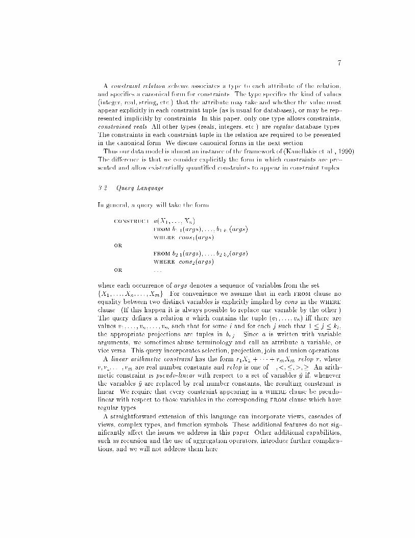
7A constraint relation scheme associates a type to each attribute of the relation,and speci�es a canonical form for constraints. The type speci�es the kind of values(integer, real, string, etc.) that the attribute may take and whether the value mustappear explicitly in each constraint tuple (as is usual for databases), or may be rep-resented implicitly by constraints. In this paper, only one type allows constraints,constrained reals. All other types (reals, integers, etc.) are regular database types.The constraints in each constraint tuple in the relation are required to be presentedin the canonical form. We discuss canonical forms in the next section.Thus our data model is almost an instance of the framework of (Kanellakis et al., 1990).The di�erence is that we consider explicitly the form in which constraints are pre-sented and allow existentially quanti�ed constraints to appear in constraint tuples.3.2. Query LanguageIn general, a query will take the formconstruct a(X1; : : : ; Xn)from b1 1(args); : : : ; b1 k1(args)where cons1(args)or from b2 1(args); : : : ; b2 k2(args)where cons2(args)or : : :where each occurrence of args denotes a sequence of variables from the setfX1; : : : ; Xn; : : : ; Xmg. For convenience we assume that in each from clause noequality between two distinct variables is explicitly implied by cons in the whereclause. (If this happen it is always possible to replace one variable by the other.)The query de�nes a relation a which contains the tuple (v1; : : : ; vn) i� there arevalues v1; : : : ; vn; : : : ; vm such that for some i and for each j such that 1 � j � ki,the appropriate projections are tuples in bi j . Since a is written with variablearguments, we sometimes abuse terminology and call an attribute a variable, orvice versa. This query incorporates selection, projection, join and union operations.A linear arithmetic constraint has the form r1X1 + � � � + rmXm relop r, wherer; r1; : : : ; rm are real number constants and relop is one of =; <;�; >;�. An arith-metic constraint is pseudo-linear with respect to a set of variables ~y if, wheneverthe variables ~y are replaced by real number constants, the resulting constraint islinear. We require that every constraint appearing in a where clause be pseudo-linear with respect to those variables in the corresponding from clause which haveregular types.A straightforward extension of this language can incorporate views, cascades ofviews, complex types, and function symbols. These additional features do not sig-ni�cantly a�ect the issues we address in this paper. Other additional capabilities,such as recursion and the use of aggregation operators, introduce further complica-tions, and we will not address them here.

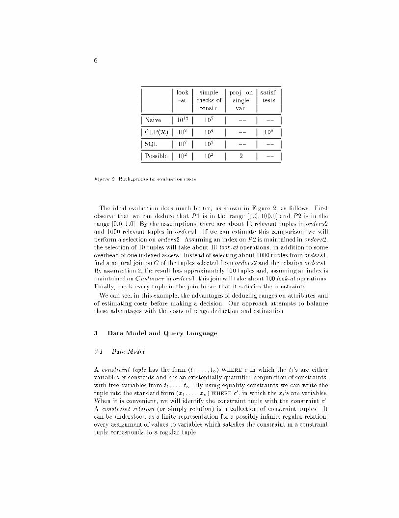
6 look simple proj. on satisf.-at checks of single testsconstr. var.Naive 1012 107 � �CLP(R) 109 104 � 106SQL 107 107 � �Possible 102 102 2 �Figure 2. Both products: evaluation costsThe ideal evaluation does much better, as shown in Figure 2, as follows. Firstobserve that we can deduce that P1 is in the range [0:0; 100:0] and P2 is in therange [0:0; 1:0]. By the assumptions, there are about 10 relevant tuples in orders2and 1000 relevant tuples in orders1. If we can estimate this comparison, we willperform a selection on orders2. Assuming an index on P2 is maintained in orders2,the selection of 10 tuples will take about 10 look-at operations, in addition to someoverhead of one indexed access. Instead of selecting about 1000 tuples from orders1,�nd a natural join onC of the tuples selected from orders2 and the relation orders1.By assumption 2, the result has approximately 100 tuples and, assuming an index ismaintained onCustomer in orders1, this join will take about 100 look-at operations.Finally, check every tuple in the join to see that it satis�es the constraints.We can see, in this example, the advantages of deducing ranges on attributes andof estimating costs before making a decision. Our approach attempts to balancethese advantages with the costs of range deduction and estimation.3. Data Model and Query Language3.1. Data ModelA constraint tuple has the form (t1; : : : ; tn) where c in which the ti's are eithervariables or constants and c is an existentially quanti�ed conjunction of constraints,with free variables from t1; : : : ; tn. By using equality constraints we can write thetuple into the standard form (x1; : : : ; xn) where c0, in which the xi's are variables.When it is convenient, we will identify the constraint tuple with the constraint c0.A constraint relation (or simply relation) is a collection of constraint tuples. Itcan be understood as a �nite representation for a possibly in�nite regular relation;every assignment of values to variables which satis�es the constraint in a constrainttuple corresponds to a regular tuple.

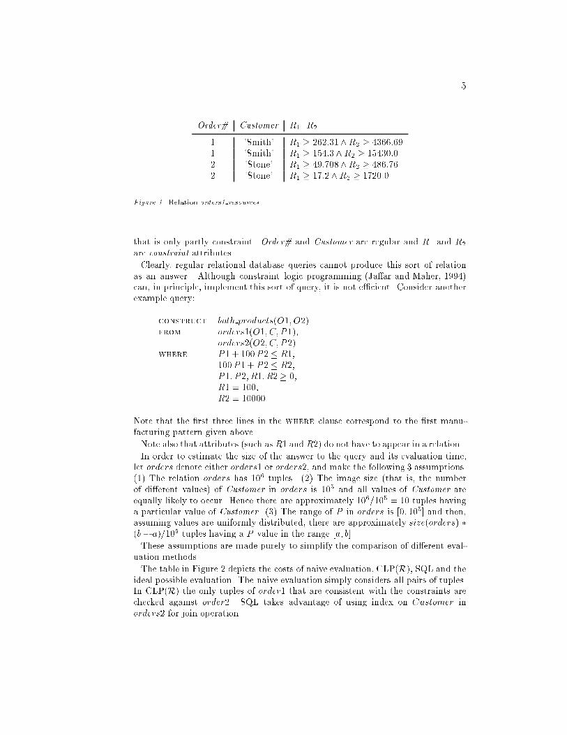
5Order# Customer R1 R21 'Smith' R1 � 262:31^R2 � 4366:691 'Smith' R1 � 154:3^R2 � 15430:02 'Stone' R1 � 49:708^R2 � 486:762 'Stone' R1 � 17:2^R2 � 1720:0Figure 1. Relation orders1 resourcesthat is only partly constraint. Order# and Customer are regular and R1 and R2are constraint attributes.Clearly, regular relational database queries cannot produce this sort of relationas an answer. Although constraint logic programming (Ja�ar and Maher, 1994)can, in principle, implement this sort of query, it is not e�cient. Consider anotherexample query:construct both products(O1; O2)from orders1(O1; C; P1);orders2(O2; C; P2)where P1 + 100P2 � R1;100P1+ P2 � R2;P1; P2; R1; R2� 0;R1 = 100;R2 = 10000Note that the �rst three lines in the where clause correspond to the �rst manu-facturing pattern given above.Note also that attributes (such as R1 and R2) do not have to appear in a relation.In order to estimate the size of the answer to the query and its evaluation time,let orders denote either orders1 or orders2, and make the following 3 assumptions.(1) The relation orders has 106 tuples. (2) The image size (that is, the numberof di�erent values) of Customer in orders is 105 and all values of Customer areequally likely to occur. Hence there are approximately 106=105 = 10 tuples havinga particular value of Customer. (3) The range of P in orders is [0; 105] and then,assuming values are uniformly distributed, there are approximately size(orders) �(b� a)=105 tuples having a P value in the range [a; b].These assumptions are made purely to simplify the comparison of di�erent eval-uation methods.The table in Figure 2 depicts the costs of naive evaluation, CLP(R), SQL and theideal possible evaluation. The naive evaluation simply considers all pairs of tuples.In CLP(R) the only tuples of order1 that are consistent with the constraints arechecked against order2. SQL takes advantage of using index on Customer inorders2 for join operation.

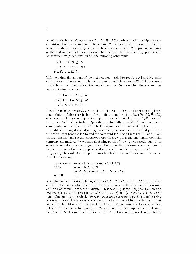
4Another relation product resource(P1; P2; R1; R2) speci�es a relationship betweenquantities of resources and products: P1 and P2 represent quantities of the �rst andsecond products respectively to be produced, while R1 and R2 represent amountsof the �rst and second resources available. A possible manufacturing process canbe speci�ed by (a conjunction of) the following constraints:P1 + 100P2 � R1100P1 + P2 � R2P1; P2; R1; R2 � 0This says that the amount of the �rst resource needed to produce P1 and P2 unitsof the �rst and the second products must not exceed the amountR1 of this resourceavailable, and similarly about the second resource. Suppose that there is anothermanufacturing processes:1:7P1 + 13:1P2 � R128:3P1+ 11:5P2 � R2P1; P2; R1; R2 � 0Now, the relation product resource is a disjunction of two conjunctions of (three)constraints, a �nite description of the in�nite number of tuples (P1; P2; R1; R2)of values satisfying the disjunction. Similarly to (Kanellakis et al., 1990), we de-�ne a constraint tuple to be a (possibly existentially quanti�ed1) conjunction ofconstraints, and constraint relation to be disjunction of constraint tuples.In addition to regular relational queries, one may have queries like: \if pro�t perunit of the �rst product is $15 and of the second is $4, and there are 100 and 10000units of the �rst and second resources respectively, what is the maximumpro�t thecompany can make with each manufacturing pattern?" or \given certain quantitiesof resources, what are the ranges of and the connection between the quantities ofthe two products that can be produced with each manufacturing process?".Typically the evaluation of queries involves both \regular" information and con-straints, for example:construct orders1 resources(O;C;R1; R2)from orders1(O;C; P1);products resources(P1; P2; R1; R2)where P2 = 0Note that in our notation the arguments O, C, R1, R2, P1 and P2 in the queryare variables, not attribute names, but we sometimes use the same name for a vari-able and an attribute when the distinction is not important. Suppose the relationorders1 consists of the two tuples (1;0 Smith0; 154:3) and (2;0 Stone0; 17:2), and twoconstraint tuples of the relation products resources correspond to the manufacturingprocesses above. The answer to the query can be computed by considering all fourpairs of tuples obtained from orders1 and from products resources. In each pair, setP1 to the value given by orders, set P2 to 0, and �nally, simplify the constraintsfor R1 and R2. Figure 1 depicts the results. Note that we produce here a relation

3There has been work on speci�c uses of constraints in databases, the earlierof which includes (Klug, 1988, Hansen et al., 1989, Chomicki and Imielinski, 1989,Brodsky and Sagiv, 1989, Maher, 1989, Ramakrishnan, 1991, Helm et al., 1991). Thepioneering work (Kanellakis et al., 1990) proposed a framework for integrating ab-stract constraints into database query languages by providing a number of designprinciples, and studied, mostly in terms of expressiveness and complexity, a numberof speci�c instances. The work of (Hansen et al., 1989) considered optimiziting inthe context arithmetic equations. However, constraint solving was limited to localpropagation and hence not suitable for LP problems. A restricted form of linear con-straints, called linear repeating points, was used to model in�nite sequences of timepoints (Kabanza et al., 1990, Baudinet et al., 1991, Niezette and Stevenne, 1992)More recent work on deductive databases (Mumick et al., 1990, Srivastava and Ramakrishnan, 1992,Kemp and Stuckey, 1993, Kemp et al., 1989, Levy and Sagiv, 1992) concentrate onoptimizing by repositioning constraints and assume the implementation of selec-tion, projection and join and optimization of expressions involving these opera-tors. Constraint algebra algorithms for speci�c constraint families was considered in(Goldin and Kanellakis, 1996) and constraint approximation-based optimization in(Brodsky and Wang, 1995). The work (Brodsky et al., 1995) proposed an approachto achieve the optimal quality of constraint and spatial �ltering. A number of worksconsider special constraint domains: integer order constraints (Revesz, 1993); setconstraints (Revesz, 1995); dense-order constraints (Grumbach and Su, 1995). Lin-ear constraints over reals drew special attention (Afrati et al., 1994, Brodsky and Kornatzky, 1995,Tollu et al., 1995, Vandeurzen et al., 1995). The use of constraints in spatial databaseswas addressed in (Paredaens et al., 1994), and to describe incomplete informationin (Srivastava et al., 1994); constraint aggregation was studied in (Kuper, 1993).The remainder of the paper is organized as follows. Motivating examples anddiscussion are next, in Section 2, and the de�nitions of our data model and querylanguage appear in Section 3. An important aspect of our work, which pertains topractical use, is the use of the notion of constraint canonical forms. Section 4 coversrelevant computational issues in constraint manipulation, which are fundamentalto constraint query evaluation. Section 5 discusses why traditional optimizationmethods are inadequate, elaborating on the discussion above. Section 6 and beyondform the core technical presentation: we deal �rst with the selection/projectionqueries in Section 6, which motivates our generic \gambling" algorithm presentedin Section 7. Section 8 gives an algorithm for sort join on constraint attributes andSection 9 presents an algorithm for �ltering multi-joins. Section 10 presents theapplication of the gambling algorithm to optimizing select-project-join queries.An earlier version of this paper was presented at the VLDB 93 conference (Brodsky et al., 1993).2. Introductory ExamplesSuppose a company manufactures two products using two resources. Its databasehas the relations orders1 and orders2 for orders of its �rst and second products re-spectively. Each relation has the attributes Order#,Customer and Product quantity.

2etc., and enable queries about design patterns that are described using constraints.LCDB technology, in particular, is important because it can enhance many exist-ing software platforms such as relational DBMS, object oriented DBMS, operationresearch packages, constraint logic programming (CLP) systems etc.Traditionally, there have been two major approaches to query optimization. Oneis based on compile-time algebraic simpli�cation of a query using heuristics as in(Hall, 1976, Minker, 1978, Pecherer, 1975, Smith and Chang, 1975, Palermo, 1974,Wong and Yousse�, 1976, Chakravarthy and Minker, 1986, Yannakakis, 1981, Bernstein and Goodman, 1981).The other is based on cost estimation of di�erent strategies as in (Astrahan et al., 1976,Gri�ths et al., 1979, Chamberlin et al., 1981, Daniels et al., 1982, Mackert and Lohman, 1986,Whang and Krishnamurthy, 1990). The heuristics of the algebraic simpli�cationapproach, such as performing selections as early as possible, assume that the se-lection conditions are readily available. In fact, extracting such conditions fromthe constraints of a query involves linear programming techniques which are, ingeneral, expensive because there may be, for example, thousands of variables. Thecost estimation approach, on the other hand, has the similar problem of extractingexplicit constraints on attributes which are needed for the estimation. Even if theseconstraints were readily available, there is a second problem: it is typically neces-sary to make assumptions about the distribution of data (like uniformity within,and independence of, attributes), and these appear unlikely to hold in LCDBs. Inshort, traditional optimization approaches are inadequate for LCDBs.In this paper, we propose a new generic approach to query optimization, that isnot only e�ective on LCDB, but also on existing query languages. The underlyingphilosophy is that expenditure of computational cost is necessary in order to obtaininformation required to estimate which is the best evaluation plan. We use statis-tical sampling for the cost estimation of speci�c plans, which has the advantageof avoiding dependence on data distribution. Since it is impractical to considerall possible plans in the search for the best one (because cost estimation of eachplan might be expensive), trials of evaluation plans are performed, one at a time,\gambling" some work required for the cost estimation of the plan in an attemptto discover a better plan. We bound the amount we can gamble, based on the bestestimated cost so far. The gambling algorithm is then used for optimization of gen-eralized select-project-join queries involving up to two generalized relations. Thisrequires to develop algorithms for estimating costs of possible evaluation plans,based on statistical methods. The problem of how to perform reasonably accu-rate and computationally cheap cost estimations for a more general class of queriesrequires more study. As additional contribution, we developed two speci�c algo-rithms: �rst, adapting the algorithm of (Edelsbrunner, 1983, Six and Wood, 1982)for n-dimensional rectangle intersection, we show how to perform an analog of thesort-join. Second, we developed a �ltering algorithm for constraint multi-join suit-able for long joins with small overall number of attributes. For a bounded numberof attributes, this algorithm provides �ltering in O(nNd logN ) time, where N is abound on the number of tuples in relations, d is the number of attributes, and n isthe number of joined relations.

, , 1?? ()c Kluwer Academic Publishers, Boston. Manufactured in The Netherlands.Toward Practical Query Evaluation for ConstraintDatabases*ALEXANDER BRODSKY [email protected]. of Information and Software Systems Engineering, George Mason University, Fairfax, VA22030, USAJOXAN JAFFAR [email protected]. of Information Systems and Computer Science, National University of Singapore, LowerKent Ridge Road, Singapore 119260MICHAEL J. MAHER [email protected] of Computing and Information Technology, Gri�th University, Nathan, 4111, AustraliaAbstract.Linear constraint databases (LCDBs) extend relational databases to include lineararithmetic constraints in both relations and queries. A LCDB can also be viewed asa powerful extension of linear programming (LP) where the system of constraintsis generalized to a database containing constraints and the objective function isgeneralized to a relational query containing constraints. Our major concern isquery optimization in LCDBs. Traditional database approaches are not adequatefor combination with LP technology. Instead, we propose a new query optimizationapproach, based on statistical estimations and iterated trials of potentially betterevaluation plans. The resulting algorithms are not only e�ective on LCDBs, butalso applicable to existing query languages. A number of speci�c constraint algebraalgorithms are also developed: select-project-join for two relations, constraint sort-join and constraint multi-join.1. IntroductionLinear programming/linear constraints is a technology widely used in applicationsof economics and business, e.g. allocation of scarce resources, scheduling produc-tion and inventory, cutting stock and many others. This paper proposes a merger oflinear programming (LP) and relational database technologies in the framework oflinear constraints databases (LCDBs), that extend relational databases to includelinear arithmetic constraints in both relations and queries. The motivation comesfrom the fact that classical LP applications do not stand alone, but rather operateover a large amount of stored data and usually require not just to optimize oneobjective function, but to answer more complex queries involving manipulation ofboth regular data and constraints. A second application realm is that of engineer-ing design systems, which may operate over large catalogs of components, devices* Much of this research was conducted while the authors were employed at the I.B.M. ThomasJ. Watson Research Center.